Embed Size (px)
Citation preview

An Analysis of Manufacturer Benefits under Vendor Managed Systems
Secil Savasaneril
Department of Industrial Engineering, Middle East Technical University, 06531, Ankara, TURKEY
Nesim Erkip 1
Department of Industrial Engineering, Bilkent University, 06800, Bilkent, Ankara, TURKEY
Vendor Managed Inventory (VMI) has attracted a lot of attention due to its benefits such as fewer stock-outs, higher sales and lower inventory levels at the retailers. Vendor Managed Availability (VMA) is animprovement that exploits the advantages beyond VMI. We complement VMA by analyzing the benefitsbeyond information sharing and by clearly assessing the motivation for the manufacturer (vendor) behindjoining to such a program. We show that such vendor managed systems provide increased flexibility inmanufacturer’s operations and may bring additional benefits. We analyze how the system parametersaffect the profitability and determine the conditions that make the vendor managed system a viablestrategy for the manufacturer.
Keywords: Vertical Collaboration; Vendor Managed Inventory; Capacity Management; Operational Flex-ibility; Consignment Stock
1 Introduction
Vendor Managed Inventory (VMI) is a collaborative process between a supplier/manufacturer and a
manufacturer/retailer/distributor, where the manufacturer gains access to the demand and inventory
information at the retailer and uses this information to “better” manage the retailer’s inventory. VMI
started as a pilot program in retail industry between Procter&Gamble and WalMart in 80’s and resulted
in significant benefits, such as lower inventory levels, fewer stock-outs and increased sales, and has been
adopted by many other supply chains such as Dell’s, Barilla’s or Nestle’s. In many research and business
articles, the benefits of VMI are attributed to information sharing between the manufacturer and the
retailer (see Cachon and Fisher 1997; Schenck and McInerney 1998). However, there is more to VMI than
just the information availability; there are benefits hidden in the increased flexibility of the manufacturer’s
production operations. There exist limited analytical work in literature on how the manufacturer can
translate this flexibility into benefit, and why the parties join to a VMI program. We believe that it is
important to emphasize the benefits of VMI additional to information sharing, so that the motivation
behind joining to a VMI program is better comprehended.
In a vendor managed setting, although the manufacturer takes control of inventory, it is the retailer that
1Corresponding author.
1

usually benefits from manufacturer managing the inventory (Dong and Xu 2002). The reason is, the
retailer can always set the terms of the agreement such that the performance measures (such as number
of stock-outs, average inventory level, etc.) will improve. Whether the manufacturer benefits from the
vendor managed system on the other hand, depends on how well the manufacturer can take advantage
of the increased flexibility. In the agreement, the retailer may reflect a required product availability
on the shelf, or service level by imposing a lower bound on the inventory level. Similarly, due to shelf
space constraints or to avoid high inventory levels, the retailer may limit the amount of replenishment
from the manufacturer. Therefore a contract may consist of an upper and a lower bound on inventory
level, where overshooting or undershooting by the manufacturer is penalized. While penalties compel the
manufacturer to conform with the inventory limits, it is definitely a challenging task for the retailer to
determine the penalties as well as to set the bounds on the inventory level that will result in the desired
service level or inventory holding cost.
Our modeling of VMI is closer to “vendor managed availability” (Hausman 2003), where the vendor
is more flexible in terms of replenishment operations than VMI, since in VMI, replenishments are more
restricted due to the bounds on retailer’s inventory level. Vendor managed availability has been practiced
by several major retailers such as J.C.Penney, or Costco. J.C.Penney supplies shirts from a Hong-Kong
based shirt-maker where the supplier completely controls the inventory by monitoring J.C.Penney’s stock
levels and making replenishments directly to the store, if necessary. To ensure availability, at times
the supplier expedites the delivery by shipping through air (Kahn 2002; Hausman 2003). Similarly,
Kimberly-Clark, a supplier of products such as diapers, tissues or paper towels for Costco in U.S., is very
flexible in its replenishment operations. The company simply “keeps each [Costco] store’s inventory as
low as possible without risking empty shelves” (Nelson and Zimmerman 2000). These examples describe
more flexible agreement terms between the manufacturer and the retailer. To reflect this practice, in our
vendor managed model we assume that the service level is the only constraint for the manufacturer, which
results in an increased flexibility even compared to VMI. For instance, at times the manufacturer may
not prefer to replenish retailer’s stock if the capacity can be used for a more profitable order. At other
times when there is excess capacity, i.e., when the capacity is less valuable, several replenishments may
enable an increased service level at the retailer. The retailer ends up with the same service level whereas
the manufacturer effectively manages its production, capacity allocation and replenishment operations.
In this paper, we consider the notions introduced by VMA, an enhanced version of VMI. In the rest of
the text, we use the terms VMA or vendor managed system to represent this enhanced version of VMI.
In this study, we model a supply chain consisting of a single manufacturer and a retailer. We first define the
traditional system under which the manufacturer and the retailer operate, and then introduce the vendor
managed system and compare the two systems. We assume that the retailer sets the terms of the contract
2
such that she is never worse off under the new (vendor managed) system. We make the analysis from the
perspective of the manufacturer who carries most of the collaboration burden. The retailer faces stochastic
demand and in the traditional system periodically places orders to the manufacturer. Manufacturer has
limited capacity to meet the orders from the retailer, and a more expensive outsourcing option. To analyze
benefits due to vendor managed system alone, our proposed model for the traditional system considers
a manufacturer that has full information on end-demand distribution, demand realization and inventory
levels at the retailer and hence revisits capacity planning aspects of operating a traditional manufacturing
system. We assume that the parties do not share cost information. Furthermore, information on available
capacity or end-of-period inventory level at the manufacturer is not shared with the retailer. Our focus
is on the vertical collaboration process in the supply chain under this asymmetric and partially shared
information setting.
In vendor managed systems the issue of who owns the inventory depends on the relationship between
the manufacturer (supplier) and the retailer (manufacturer). If the manufacturer is very powerful (such
as Dell) it may force the suppliers to own the inventory at the manufacturer’s site or at a supply hub
nearby. On the other hand, if supplier is powerful then inventory may not be consigned. Intel, for
instance, although has an agreement with Dell, does not operate through supply hub like other suppliers
(Barnes et al. 2000). We consider two types of vendor managed agreements, consignment stock and
no-consignment stock, and for each type analyze how the manufacturer may benefit from managing the
retailer’s inventory. In our model there does not exist an upper and lower bound restriction at the
retailer’s inventory level; however retailer explicitly specifies service level and average inventory level
requirements. Given this setting we address the following questions: (i) Are there any benefits for the
manufacturer in managing the retailer’s inventory apart from what is already achieved by sharing demand
and inventory information? (ii) What are the conditions that make the manufacturer better off under the
vendor managed system considered? (iii) Under the vendor managed system should the manufacturer
consign the stock or not?
Our work contributes to the literature in several ways. Our work is one of the few studies that analyzes
benefits due to vendor managed systems from the manufacturer’s perspective and that identifies the
conditions to make the manufacturer willing to join such an agreement. Earlier studies either ignore
the motivation behind vendor managed systems, or focus only on total supply chain benefits rather
than the individuals’. Furthermore, we make a comparison of benefits under consignment stock and
no-consignment stock models, to determine the type of agreement the manufacturer will benefit, whereas
previous literature mostly assume centralized, consignment stock models.
The remainder of the paper is organized as follows. In §2 we review the previous work on vendor managed
inventory systems. In §3 and §4 the model characteristics and structural properties are presented. In
3
§5 we make an experimental analysis and discuss the results, and based on these discussions we provide
managerial insights. We present our conclusions in § 6.
2 Literature Review
Majority of existing studies analyze the vendor managed system in a manufacturing-retailer setting,
while a few consider a supplier-manufacturer setting (Choi, Dai and Song 2004). Inventory ownership is
modeled either by totally consigned stock, or by the transfer of the title at the time of arrival. In most
of the previous studies, the focus of the analysis is limited to designing an optimal operating policy for
the vendor in a vendor managed system, and the motivation of the vendor in managing the inventory is
not under consideration.
In the analysis of the vendor managed systems under a single manufacturer and multiple retailers, the
focus is mainly on the savings in transportation due to better order consolidation or savings due to co-
ordination of retailer replenishments. To analyze the benefit of VMI, Cetinkaya and Lee (2000) compare
a VMI system with a traditional system. In the traditional system the manufacturer sends a shipment
immediately when the demand arrives, while in VMI system shipments are consolidated. Authors de-
termine the optimal dispatch quantity under VMI considering the inventory cost and the transportation
cost incurred by the manufacturer, and conclude that when inventory holding cost and dispatching cost
are low, VMI results in significant savings for the manufacturer. Kleywegt, Nori and Savelsberg (2002)
study an inventory routing problem of a manufacturer who owns the inventory at the retailers. An
approximation method is developed to find the minimum cost routing policy, however, there does not
exist a discussion on whether the manufacturer is better off under the vendor managed system. Waller,
Johnson and Davis (1999) also consider a multiple retailer setting and through a simulation analysis
demonstrate the effects of VMI on the inventory levels at the retailers and on the capacity utilization at
the manufacturer. VMI results in savings due a decrease in the inventory levels, which is a consequence
of the increased frequency of retailer replenishments. Aviv and Federgruen (1998) consider a capacitated
supplier with multiple retailers and analyze how coordination of retailer orders under VMI decrease the
system-wide cost of operation. They explicitly model a traditional system with no information sharing
and with full information sharing to assess the benefits of VMI beyond information sharing.
Fry, Kapuscinski and Olsen (2001) compare a VMI system with a traditional system in a single manufac-
turer, single retailer setting under full information sharing. The authors identify the optimal operating
policies of both the manufacturer and the retailer in a stochastic setting. Under VMI the retailer de-
termines the maximum inventory level and the vendor incurs a penalty if the inventory level is outside
the limits. Authors find that VMI performs close to a centralized model in the presence of high demand
4

variance and high cost of outsourcing. Several other papers study the optimal decisions of the manu-
facturer under VMI in a deterministic environment. Valentini and Zavanella (2003) and Shah and Goh
(2006) consider a consignment stock system where the demand is deterministic with a constant rate.
Jaruphongsa, Cetinkaya and Lee (2004) study a problem with delivery time windows and early shipment
penalties under dynamic demand. The authors propose a dynamic programming algorithm to obtain the
minimum cost under VMI.
Depending on the form of agreement between the retailers and the manufacturer, the system under vendor
managed regime can be very close to a centralized system. A number of papers analyze the role of VMI
as a channel coordinator. Bernstein, Chen and Federgruen (2006) study the constant wholesale price and
quantity discount contracts that lead to perfect coordination in a supply chain with multiple competing
retailers, and show how VMI helps achieve the coordination. Nagarajan and Rajagopalan (2008) show
that simple contracts in VMI can improve the performance of the overall system under certain conditions.
Dong and Xu (2002) analyze the benefits of VMI both in terms of total channel cost and vendor’s cost.
In their model the retailers set the purchasing price in the contract and the supplier in turn determines
the selling quantity. Authors determine the conditions under which the supplier benefits from VMI and
conclude that VMI can always decrease the cost of channel as a whole. Fry, Kapuscinski and Olsen (2001)
also discuss centralization of the supply chain.
There has been few work on the service level considerations in a VMI system. In most of the papers
the service level is assumed implicit in the lower inventory level set by the lower-echelon. Choi, Dai
and Song (2004) study the service level relationship between a supplier and a manufacturer in a VMI
framework and show that high service levels at the supplier does not guarantee the desired service level
at the manufacturer and that expected backorders should also be taken into account.
Our study is most closely related to Fry, Kapuscinski and Olsen (2001). We study a single manufacturer
single retailer system and compare the vendor managed system with the traditional system to quantify
the benefits beyond information sharing. However, we focus on the benefits to the manufacturer to
determine the motivation to make an agreement. We furthermore consider capacity management as an
important factor in determining the benefits of vendor managed system. Additionally, we study both
consignment and no-consignment models to identify the conditions that make either model beneficial for
the manufacturer. In our model, we do not necessarily regard the vendor managed system as a coordinated
system. We propose a more realistic setting with asymmetric and partial information sharing and focus
on the collaboration process. Since usually it is the manufacturer that is reluctant in these agreements,
we analyze the problem from manufacturer’s perspective. Finally, we take service level considerations
explicitly into account.
In summary, our model differs from the existing studies in the following aspects: (i) We look at manufac-
5

turer benefits in joining to the vendor managed system. (ii) We identify the benefits beyond information
sharing to clearly assess the manufacturer’s motivation. (iii) We explicitly model the consignment and
no-consignment systems and provide a comparison of these systems to determine which type of agree-
ment is more beneficial to the manufacturer. In practice, if the lower echelon is more powerful, the stock
is usually consigned by the manufacturer. Otherwise, if the manufacturer is powerful, the stock is not
necessarily consigned. Therefore it is not apparent whether the manufacturer should consign the stock or
not. (iv) Finally, we analyze how benefits under vendor managed system change with system parameters.
Specifically, we measure the effect of capacity management and provide a detailed analysis of the benefits
from production and transportation flexibility.
3 A Modeling Framework for the Manufacturer
We compare two settings; a traditional system where the retailer manages and owns the inventory, and
a vendor managed system. In the vendor managed system we model two cases based on the ownership
of stock. Under no-consignment stock model (VM-NC), the stock is managed by the manufacturer while
owned by the retailer. Under consignment stock model (VM-C), the inventory is both managed and owned
by the manufacturer. We assume the retailer accepts the agreement only if the performance measures
are as good compared to the traditional case.
We consider a periodic-review model where the manufacturer has limited and non-stationary capacity,
which is known by the manufacturer in advance. The non-stationarity in the capacity reflects an envi-
ronment where the manufacturer has several customers and allocates some portion of the capacity to the
retailer and the remaining to the other orders. We assume that the capacity allocated to the retailer may
be 0 in some periods, i.e., the manufacturer produces for the retailer in every Tp periods, and without loss
of generality we assume non-negative capacity in the first period of Tp. We call the time span between
two positive capacity levels as the production cycle. Note that cyclic production concept is a well-known
and utilized idea in the literature. Maxwell and Muckstadt (1985) introduced the idea of consistent and
realistic reorder intervals. Li and Wang (2007) mention cyclic structures within the supply chain as a
coordination mechanism. Fry, Kapuscinski and Olsen (2001) consider a similar cyclic structure in their
study. We further assume that the level of capacity may be non-stationary for the periods in which the
manufacturer produces for the retailer. We assume this non-stationarity also shows a cyclic behaviour.
In other words, in every Tm periods the level of the capacity is the same and Tm may consist of several
Tp cycles, each cycle with possibly a different capacity level (see Figure 1). We call this larger cycle as
the capacity cycle. Similarly, due to scheduling practices the retailer places a replenishment order to the
manufacturer in every Tr periods. We call the retailer’s cycle as the replenishment cycle.
6

Periods
Capacity allocated to the retailer
Production cycle
Capacity cycle
Replenishment cycle
Figure 1: Manufacturer’s capacity cycle is 12 periods, production cycle is 6 periods, retailer’s replenish-ment cycle is 4 periods.
We assume the replenishment orders are quantized, where unit replenishment size Q reflects economies of
scale in manufacturing and transportation and is an agreed-upon quantity between the manufacturer and
the retailer. Note that, this assumption implies that the manufacturer is expected to operate with this
“bucket” size Q with all of the customers. Hence, we can assume that the capacity at the manufacturer is
a non-negative integer multiple of Q. This type of environment can be observed in practice. For example,
DMC, a French thread company, lowered its shipment size from 24-unit cases to 12-unit cases after an
agreement made with WalMart. Since switching to 12-unit case required significant investment now the
company is shipping in 12-unit cases to all of its customers (Fishman 2006).
The end-item demand is stochastic and stationary. Holding cost is incurred based on end-of-period
inventory level, and the retailer operates based on a service level constraint. Excess demand at the retailer
can be backlogged (there is no cost associated), however the manufacturer (always) meets the retailer
order either through regular stock or by subcontracting (for a similar usage of subcontracting option,
see Gavirneni, Kapuscinski and Tayur 1999). Here, the term “subcontracting” actually corresponds to
a variety of alternatives to meet the unsatisfied demand. The manufacturer can use an additional “set
up” from the capacity of other products/customers, overtime production, expedite the supply, or let the
retailer to take care of unmet demand but pay a(n implied) penalty. We assume that transportation time
is negligible and hence the produced amount is delivered at the same period (overnight). Note that this
is consistent with the JIT delivery concept.
We model the retailer’s and the manufacturer’s problem under the traditional system, and the manufac-
turer’s problem under the vendor managed system as a Markov Decision Process (MDP). We determine
the optimal operating policy under each system. Model parameters, decision variables and state variables
are presented in Table 1.
One of the objectives of this study is to quantify the benefits of the vendor managed system for the
7

manufacturer when demand and inventory information of the retailer is available. Specifically, we make
the following assumptions on information sharing:
1. The information of periodic demand realization, end-of-period inventory level at the retailer, and
retailer’s demand distribution is provided by the retailer to the manufacturer.
2. Information of unit inventory holding cost or any other cost information at the retailer is not
shared with the manufacturer. Similarly, cost information of the manufacturer is not shared with
the retailer. Cost information is mutually unavailable.
3. Information on capacity level and end-of-inventory level at the manufacturer is not shared with the
retailer. Therefore information sharing is asymmetric and partial.
Table 1: Notation for Traditional and Vendor Managed System Models
Parameters
Tp: length of the production cycle for the manufacturerTm: length of the capacity cycle for the manufacturerTr: length of the replenishment cycle for the retailer under traditional systemDi: random variable denoting demand over i periods, i ∈ {1, · · · , Tr}Pi: probability mass function for Di
Q: batch order (dispatch) quantityc: unit production costw: unit outsourcing costh: (manufacturer’s) unit holding cost
1 − β: service level at the retailerz: the number of production cycles in a capacity cycle, zTp = Tm
Decision Variables
R: reorder level at the retailerpn: number of lots of Q produced in period ndn: number of lots of Q dispatched in period n
State Variables
Inm: number of lots on-hand at the manufacturer at the end of period n − 1,
Inm ∈ {0, 1, · · · ,∞}.
Inr : net inventory at the retailer at the end of period n − 1,
Inr ∈ {−∞, · · · ,∞}.
tnm : the relative position of period n in capacity cycle,tnm ∈ {1, · · · , Tp, · · · , 2Tp, · · · , zTp = Tm}
tnr : the relative position of period n in replenishment cycle,tnr ∈ {1, · · · , Tr}
Kn : the capacity level in period n (implied by tnm),Kn ∈ {0, K1, · · · , Kz}.
ST : state under traditional system, ST = (Im, Ir, tm, tr)SNC : state under no-consignment vendor managed system, SNC = (Im, Ir, tm)
SC : state under consignment vendor managed system, SC = (Ir, tm)
8

3.1 Traditional System
In the traditional model, at the beginning of each period the manufacturer decides on how much to
produce and/or to outsource. The manufacturer produces for the retailer in every Tp periods, while the
retailer places an order in every Tr periods. Tr is known by the manufacturer. We assume that fixed
cost of transportation is zero under traditional and under vendor managed systems. We assume that the
retailer places orders based on an (R, nQ) type policy, where R is the reorder point that guarantees a
specified service level (Zheng and Chen 1992). Note that due to quantized shipments the analysis would
not change under a fixed cost of transportation per batch. The sequence of events under traditional
system is as follows:
1. At the beginning of a period, the manufacturer gives the decision of how many units to produce
and/or to outsource, considering the allocated capacity (if allocated capacity is zero, there is no
production). If an order is placed by the retailer in the last period of the replenishment cycle, a
dispatch is made to the retailer in the first period of the following replenishment cycle. Production,
outsourcing and dispatch lead times are negligible. Therefore the dispatched quantity is immediately
ready at the retailer at the beginning of the replenishment cycle, before any demand is realized at
the retailer.
2. Demand is realized at the retailer. If there is enough inventory in stock, the retailer fulfills the
demand. If the retailer can not meet the demand completely, the unmet amount is backordered (at
no explicit penalty). If it is the last period of the replenishment cycle, the retailer places an order
at the manufacturer (if any), which is a non-negative integer multiple of Q. Otherwise, if it is not
the last period, the retailer only passes the demand information to the manufacturer, and updates
the inventory level.
3.1.1 Retailer’s problem under the traditional system
The problem of the retailer is to minimize the expected inventory level under a service level requirement
(there is no explicit backorder cost for the retailer). We only consider the operating policies with (R, nQ)
structure. In the last period of the replenishment cycle, after the demand is realized, retailer places an
order if the inventory level is equal to or less than the reorder point, R. The reorder point, R, is the
decision variable and Q is assumed to be a parameter.
First, consider the two measures for a given R and Q: (i) Expected average inventory level (I), and (ii)
Average service level (1 − β).
9

The expected average inventory level is expressed as follows:
I =1
Q
R+Q∑
i=R+1
i∑
j=0
(i − j)P1(j) + P2(j) + · · · + PTr
(j)
Tr(1)
In (1), P1 is the probability mass function of single period demand and Pk, k ∈ {1, · · · , Tr}, is the k-
convoluted probability mass function (i.e., probability mass function of k-period demand). Consider the
replenishment cycle Tr. Under the quantized ordering policy, (R, nQ), at the beginning of each cycle the
inventory level at the retailer is i with probability 1Q , where i ∈ {R + 1, · · · , R + Q}. In the long-run,
for the first period of the cycle, expected end-of-period inventory level is 1Q
∑R+Qi=R+1
∑ij=0(i − j)P1(j),
Similarly, for the second period, expected end-of-period inventory level is 1Q
∑R+Qi=R+1
∑ij=0(i − j)P2(j),
and so on. Since in the long-run, probability of being in any period in the replenishment cycle is equal
to 1Tr
, the time-averaged expected inventory level is expressed as in (1).
We define the average service level as 1 − β, where β is the expected average fraction of backordered
demand per period. Let βi, i = 1, 2, · · · , Tr, denote the expected fraction of backordered demand in the
ith period of the replenishment cycle. Then βi would be expressed as follows:
βi =∑
Ii
P (Ii)E[(D1 − Ii)
+]
E[D1]
where Ii is the beginning inventory level of the ith period, P (Ii) is the probability that the beginning
inventory level is Ii, and D1 is the random variable denoting one-period demand. Then expected average
fraction of backordered demand, β, is expressed as:
β =β1 + β2 + · · · + βTr
Tr(2)
Equivalently, β is expressed as follows:
β =1
Q
R+Q∑
i=R+1
∞∑
j=i+1
(j − i)PTr
(j)
TrE[D1]. (3)
We limit the operating policy of the retailer to the (R, nQ) policy. Under this policy, to minimize the
expected average inventory level in (1), the retailer simply chooses the minimum reorder point that
guarantees the desired service level. However, as we analyze below, under quantized ordering (R, nQ)
type policy is not necessarily the optimal policy for the retailer. In other words, even if the optimal
reorder point is chosen, expected inventory level may not be minimized. In Proposition 1 below, we
identify the conditions under which the optimal policy is indeed an (R, nQ) type policy for Tr = 1. We
present the proofs in Appendix.
Each reorder point implies a service level (1 − β), and an expected inventory level (I). Let S be the set
of the β values implied by all (integer and non-negative) reorder points (note that the elements of set S
10

vary with Q). For β ∈ S, let R(β) denote the reorder point that results in the service level of 1− β. (We
assume there exists a unique R(β) for each β ∈ S. Under Tr = 1 this is possible if R(β) + 1 ≤ max(D1)).
Proposition 1 Suppose Tr = 1.
(i) For β ∈ S, (R(β), nQ) policy is the unique inventory level minimizing policy for the retailer.
(ii)For β 6∈ S, there may exist more than one optimal ordering policy for the retailer, none of which is
an (R, nQ) policy.
Proposition 1 implies that for β ∈ S the only policy that achieves the minimum inventory level is
(R(β), nQ) policy. We use this result later in Section 4 when analyzing the manufacturer’s policy.
3.1.2 Manufacturer’s problem under the traditional system
We determine the optimal operating policy of the manufacturer under the traditional system. We model
the manufacturer’s problem as a Markov Decision Process under average cost criteria as follows.
g(s) = minδ
limN→∞
1
NEδ
s
[
N∑
n=1
r(sn, an)]
(4)
where g(s) indicates the optimal average cost given that initial state is s, δ is any Markovian policy (note,
the underlying chain is weakly communicating and under average cost criteria an optimal policy exists),
sn indicates the state in period n, an indicates the action in period n, and r(sn, an) is the (immediate)
cost of taking action an in state sn. We define the states under traditional model as, ST = (Im, Ir, tm, tr)
where,
Im is the number of lots on-hand at the manufacturer at the end of the previous period, or at the
beginning of the current period. Since capacity in every period is a non-negative integer multiple of
Q, without loss of optimality, Im indicates a non-negative integer multiple of Q, Im = {0, 1 · · · ,∞}.
If Im = 2 for instance, there exists 2Q units in inventory (see the discussion on action space).
Ir is the net inventory at the retailer at the end of the previous period, Ir = {−∞, · · · ,∞}.
tm denotes the relative position of a period in the capacity cycle, tm ∈ {1, · · · , Tm}. We assume Tm
implies the following capacity structure, (K1, 0, 0, · · · , 0, K2, 0, 0, · · · , 0, Kz, 0, 0, · · · , 0)
tr denotes the relative position of a period in the replenishment cycle, tr ∈ {1, · · · , Tr}.
In the traditional model, the action is defined only by the production quantity in period n, pn. The
quantity to be outsourced can already be inferred from the retailer’s order quantity at the end of the
replenishment cycle. If the order quantity exceeds the amount in stock and the production capacity of
11

the manufacturer, then the remaining quantity should be outsourced. This implies outsourcing is not an
independent decision. Note that outsourcing takes place only at the beginning of the replenishment cycle,
since otherwise it will result in additional holding cost. The retailer orders in multiples of Q, and capacity
available is a multiple of Q, therefore without loss of optimality, we limit the production quantity in every
period to multiples of Q (this implies Im is a multiple of Q). The action space in a period is denoted by
pn ∈ {0, 1, · · · , Kn}, where each value corresponds to the multiple of Q. We assume that single period
demand is characterized by a discrete probability distribution.
Next, we define the components of Equation (4) under the traditional model. We define r(s, a), where
s = (Inm, In
r , tnm, tnr ) and a = (pn), as follows:
r(s, a) =
(
cpn + h(Inm + pn − L)+ + w(−In
m − pn + L)+)
Q if tnr = 1(
cpn + h(Inm + pn)
)
Q if tnr 6= 1(5)
where L denotes the number of lots requested by the retailer at the end of replenishment cycle, i.e., at
the end of period Tr. The amount requested is dispatched by the manufacturer in the first period of the
replenishment cycle, and is ready at the retailer before the demand is realized. Note that, the quantity
L is deterministic and can be inferred from Ir.
Transition probability P (j|s, a) denotes the probability that next state is j given current state is s and
action taken is a, where j = (In+1m , In+1
r , tn+1m , tn+1
r ). We categorize all possible transitions under the
traditional system as follows:
For tnr 6= 1,
P (j|s, a) =
P1(Inr − In+1
r ) if
In+1m = In
m + pn,tn+1m = tnm(1 − 1{tm=Tm}) + 1,
tn+1r = tnr (1 − 1{tr=Tr}) + 1
0, otherwise
where 1{tm=Tm} takes value of 1 for the last period of the capacity cycle. P1(Inr − In+1
r ) is the probability
that single period demand is Inr − In+1
r .
For tnr = 1 there are two possibilities. The retailer’s order quantity does not exceed the available stock and
production quantity, and therefore outsourcing is not necessary. When this is the case, Inm+pn−In+1
m = L.
Otherwise, if outsourcing is necessary, then In+1m = 0. We present the transition probability as follows.
P (j|s, a) =
P1
(
Inr − In+1
r + LQ)
, if
In+1m = (In
m + pn − L)+
tn+1m = tnm(1 − 1{tm=Tm}) + 1,
tn+1r = tnr + 1
0, otherwise
12

3.2 Vendor Managed System
Under the vendor managed system, we focus only on the manufacturer’s problem since the retailer
does not make any decisions. Retailer only requires her performance measures to be as good as those
under the traditional system. At the beginning of the production cycle the manufacturer decides on
how much to produce, and in every period how much to outsource and to dispatch. The dispatched
quantity immediately arrives at the retailer, i.e., lead time of transportation is zero. Note that due to
the agreement there does not exist a replenishment cycle. The sequence of events is as follows:
1. At the beginning of a period, the manufacturer gives the decision of how many units to produce (if
possible), to outsource and to dispatch. Inventory status of the manufacturer and the retailer are
updated based on the dispatch quantity.
2. The demand is realized at the retailer’s site. Inventory status of the retailer is updated and end-
of-period holding costs at the manufacturer and at the retailer are incurred.
We analyze the vendor managed setting under two cases; no-consignment stock and consignment stock.
3.2.1 No-consignment stock
Under no-consignment stock model (VM-NC) the ownership of the stock is transferred to the retailer
once the dispatch arrives at the retailer. To be compatible with the traditional system, we assume that
under the vendor managed system the retailer requires the average inventory investment to be as low as,
and average service level to be as high as those levels under the traditional system. In other words, the
retailer is indifferent between the traditional and the vendor managed system.
We determine the manufacturer’s optimal operating policy under the no-consignment system. We model
the manufacturer’s problem as a Markov Decision Process under the average-cost criteria as follows:
g(s) = minδ
limN→∞
1
NEδ
s
[
N∑
n=1
r(sn, an)]
(6)
s.t. Average Inventory Level at Retailer ≤ I (7)
Service Level at Retailer ≥ 1 − β (8)
where β is defined as in (3), and I as in (1). The constraint on inventory level in (7) reflects the case where
the retailer is not willing to pay for inventory investment more than what it pays under the traditional
system. In practice, the retailer may require that at least one of the performance measures described by
Equation (7) or (8) are improved as a result of the agreement. Hence the service level specified by (1−β)
13

can be regarded as a lower bound, and similarly the limit specified by I on the average inventory level
under vendor managed system can be regarded as an upper bound.
In all our analysis, right-hand-side (RHS) of Equation (7) or (8) is used as is, so that we have comparable
cases. Note that it is through these constraints that the availability is ensured at the retailer at the right
level of inventory. If instead, the retailer were to operate with min-max bounds on inventory, compared
to the traditional system the retailer’s either the service level would be lower or average inventory level
would be higher or both. Furthermore, the manufacturer’s benefits would decrease due to decreased
operational flexibility.
The state is SNC = (Im, Ir, tm) where Im, Ir, and tm are as defined in Table 1. At the beginning of
the production cycle the manufacturer decides on how much to produce, pn, and in every period how
much to outsource, yn, and to dispatch, dn. The manufacturer produces, outsources and dispatches in
multiples of Q, and capacity available at the beginning of the production cycle is a multiple of Q. The
action space is denoted as, pn ∈ {0, 1, · · · , Kn} and dn ∈ {0, 1, · · · ,∞}. Without loss of optimality, we
limit the action space to multiples of Q. Note that the outsourced quantity at period n, yn, is defined by
(dn − Inm − pn)+, and is not a(n independent) decision variable.
Next, we define the components of Equations (6) through (8). In (6) we define r(s, a), where s =
(Inm, In
r , tnm) and a = (pn, dn), as follows:
r(s, a) =(
c.pn + h(Inm + pn − dn)+ + w(−In
m − pn + dn)+)
Q (9)
Note that L in Equation (5) is now a decision variable and is denoted with dn. We define transition
probabilities, P (j|s, a) where j = (In+1m , In+1
r , tn+1m ), as follows:
P (j|s, a) =
P1(Inr − In+1
r + dnQ), ifIn+1m = (In
m + pn − dn)+
tn+1m = tnm(1 − 1{tm=Tm}) + 1,
0, otherwise
Left-hand-side (LHS) of (7) reflects the expected inventory level per period at the retailer under the
manufacturer’s optimal operating policy and is expressed as:
∑
Im,tm
∑
i>0
iπMNC(Im, Ir = i, tm).
where πMNC(Im, Ir = i, tm) is the fraction of time spent (or the steady-state probability) in state (Im, Ir =
i, tm) under the manufacturer’s optimal operating policy under no-consignment system. LHS of (8)
reflects the average service level at the retailer under the manufacturer’s optimal operating policy:
1−∑
Im,i,tm
∑
d(i):i+d(i)>0
πMNC(Im, Ir = i, tm)
E[(D1 − i − d(i))+]
E[D1]−
∑
Im,i,tm
∑
d(i):i+d(i)≤0
πMNC(Im, Ir = i, tm)
E[D1]
E[D1].
14

(10)
In (10) d(i) denotes the set of possible dispatch actions that can be taken at state i. In the expression
note that expected backordered demand is calculated differently if i + d(i) ≤ 0. When i + d(i) > 0, the
amount of available stock at the retailer before the demand is realized is positive. Then the expected
backordered demand is E[(D1 − i− d(i))+]. On the other hand, if i + d(i) ≤ 0, then all demand occurred
in that period should be backordered and expected backordered demand is E[D1]. For those periods
service level is 1 − E[D1]E[D1]
= 0. Averaging over all periods gives the expression in (10).
Finally, we note that if under optimal dispatch policy the available stock at the retailer before the demand
is realized is always positive, then service level is always positive in all of the periods. When this is the
case, the service level expression in (10) can be replaced with the following expression:
∑
Im,tm
∑
i<0
|i|
E[D1]πM
NC(Im, Ir = i, tm). (11)
3.2.2 Consignment Stock
In the consignment stock system (VM-C) the sequence of events is the same with no-consignment system
except that the manufacturer owns and manages the inventory at the retailer’s site. We determine the
manufacturer’s optimal operating policy under the consignment system. We model the manufacturer’s
problem as a Markov Decision Process under average cost criteria as follows:
g(s) = minδ
limN→∞
1
NEδ
s
[
N∑
n=1
r(sn, an)]
(12)
s.t. Service Level at Retailer ≥ 1 − β (13)
Note that since the stocking cost is incurred by the manufacturer there does not exist any constraint
on the average inventory level. Furthermore, as we describe below, the reward function, r(s, a), now
includes the holding cost at both the manufacturer and the retailer. Observe that Equation (13) is same
as Equation (8).
In the consignment stock model, we assume that unit holding cost is the same at the manufacturer’s
and the retailer’s site. The carrying charge of the inventory at a site is determined by the opportunity
cost and risk level at the site. Since stocks at both echelons belong to the same firm (manufacturer), the
opportunity costs of the tied up capital that could be used in some other investment is the same at both
sites. Furthermore, the risk levels at both sites are the same, since the manufacturer has a single retailer.
If there were multiple retailers, the manufacturer would prefer to keep stock at the upper echelon to
minimize the risks and send the items to lower echelon only when necessary. Due to increased risks, the
implied unit holding cost at the lower echelon would be higher. However, in this single retailer setting
15

keeping the items at the lower echelon rather than at both echelons does not affect the inventory holding
cost while improving the service level.
Since unit holding cost is the same at manufacturer’s and retailer’s site, the manufacturer keeps inventory
only at the retailer’s site and as a result immediately dispatches whatever it produces and outsources to the
retailer’s site. Under consignment stock the state is defined as SC = (Ir, tm) where Ir and tm are defined
as before, and the actions are only how much to dispatch at the beginning of period n, dn ∈ {0, 1, · · · ,∞},
where each dn value corresponds to the multiple of Q.
We define r(s, a) where s = (Inr , tnm) and a = (dn), as follows:
r(s, a) =(
c.min{dn, Kn} + w. max{dn − Kn, 0})
Q + hE[(Inr + dnQ − D1)
+]. (14)
Note that in r(s, a) the holding cost at the manufacturer’s site is not expressed, since stock is kept only
at the retailer’s site. The transition probabilities are expressed as follows:
P (j|s, a) =
{
P1(Inr − In+1
r + dnQ), if tn+1m = tnm(1 − 1{tm=Tm}) + 1
0, otherwise
The consignment and no-consignment models are different but related. Note that in the Markov Decision
Process the reward functions and the constraints are different (see Equations (6)-(9) and (12)-(14)).
However, the two systems are related in that there are parameter settings under which the actions taken
under both systems are the same. Note that Equation (7) in the no-consignment model implies a unit
holding cost. If the implied holding cost is equal to the manufacturer’s holding cost, h, then consignment
and no-consignment system can be regarded as equivalent in terms of the actions taken. For tighter or
more relaxed inventory restrictions consignment and no-consignment systems are expected to result in
different operating policies.
4 Analysis and comparison of traditional and vendor managed systems
In this part, we first provide an analysis on the structural properties of the optimal policy under traditional
and no-consignment systems. Then we compare the cost under no-consignment system with the cost under
traditional system and the cost under consignment system. In the remainder of the text, we denote
traditional system with TRAD, no-consignment vendor managed system with VM-NC, and consignment
system with VM-C.
4.1 Structural properties of the optimal policy
We analyze the structural properties of the optimal policy under traditional and under no-consignment
systems. We show in Property 1 that the optimal policy under the traditional system is a modified
16

base-stock policy. For the no-consignment system, we discuss how the retailer’s optimal policy and
the resultant inventory level and service level constraints affect the manufacturer’s optimal policy. In
Property 2 we show that under certain conditions, the optimal policy under no-consignment system is
also a modified base-stock policy.
Property 1 Optimal policy of the manufacturer under traditional system is a modified base-stock policy.
Next, we discuss optimal operating policy of the manufacturer under VM-NC. Under VM-NC the man-
ufacturer decides on how much to produce, outsource and dispatch to the retailer’s site. The dispatch
policy is subject to the following two constraints: (i) Expected inventory level at the retailer can not
exceed a certain level (as expressed in (7)), and (ii) Service level at the retailer should satisfy a minimum
level (as expressed in (8)). These constraints make it difficult to characterize the optimal operating policy
of the manufacturer. However, as we show in Property 2 under certain conditions the optimal policy of
the manufacturer has the rather simple base-stock structure.
To define the manufacturer’s policy under VM-NC, we should focus on the retailer’s operating policy
under the traditional system. In Proposition 1 we show that when Tr = 1, for β ∈ S there exists a unique
optimal policy which is (R(β), nQ). This result leads to the following observation.
Observation 1 For Tr = 1 and β ∈ S:
(i) Under VM-NC the manufacturer’s optimal operating policy is defined by a unique dispatch policy.
This unique dispatch policy is the same policy as the retailer’s order policy under the traditional system,
which is (R(β), nQ).
(ii) Manufacturer’s optimal operating policy under VM-NC is independent of β.
Observation 1 states that for β ∈ S, under optimality the only possible dispatch policy of the manufacturer
that satisfies constraints (7) and (8) is the retailer’s (R(β), nQ) policy. In other words, in every period
the manufacturer dispatches the minimum amount (in multiples of Q) to bring the retailer’s stock level
above R(β). Furthermore, the dispatch policy is the same for all β ∈ S. The reason is, discrete reorder
points define β and the value of the reorder point does not have an impact on the dispatch policy of
the manufacturer (This structure resembles the one in a base-stock system where the order-up-to point
does not affect the quantity ordered every period). For β 6∈ S, multiple dispatch policies may satisfy
the constraints (7) and (8). Under optimality the manufacturer may select one of the eligible dispatch
policies. Using Observation 1, in Property 2 we provide a characterization of the optimal policy of the
manufacturer.
Property 2 For Tr = 1 and β ∈ S, under VM-NC the manufacturer’s optimal policy is a modified
base-stock policy.
17

4.2 Comparison of traditional and vendor managed systems
In this section we make two comparisons. First, we compare the no-consignment system with the tra-
ditional system. Using the structural results of the previous subsection, we show that the cost under
the no-consignment system is always lower than or equal to the cost under the traditional system (Prop-
erty 3). We then compare the no-consignment system with the consignment system. In Proposition 4
we show that under certain settings and under certain sufficient conditions the cost of the consignment
system is lower than the cost of the no-consignment system.
4.2.1 Comparison of no-consignment and traditional systems
Property 3 The cost of the manufacturer under VM-NC is always lower than or equal to the cost under
TRAD.
Property 3 states that if under vendor managed system stock is not consigned, then vendor managed sys-
tem results in lower cost than the traditional system, i.e., VM-NC is a no-risk case for the manufacturer.
4.2.2 Comparison of no-consignment and consignment systems
Although VM-NC is a no-risk case, the cost under VM-NC is not always lower than the cost under VM-C.
As we show in the analysis below, under vendor managed system consigning the stock may be less costly
than not consigning it. In the following, we introduce a specific instance. For this instance, we first obtain
a lower bound on the optimal cost under VM-NC (Proposition 2), and an upper bound on the optimal
cost under VM-C (Proposition 3). We then identify a set of sufficient conditions that make VM-C less
costly than VM-NC (Proposition 4).
Assume that Q = 1 and that the (single-period) demand, D, has the following probability distribution:
P (D) =
{
1/2, if D = µ − 11/2, if D = µ + 1
Assume that capacity per period is E[D] = µ, and Tr = 1, i.e., under the traditional system retailer
places orders in every period. In the analysis below, we focus on the cases where β ∈ S. In this setting
since Q = 1, under the traditional system the retailer operates under the base-stock policy.
Proposition 2 For the instance defined above, LB(VM-NC) =√
(w − c)h − h2 + cµ is a lower bound
on the manufacturer’s optimal cost under VM-NC.
In the following, we determine an upper bound on the optimal cost of the manufacturer under VM-C
(Proposition 3). Under VM-C the manufacturer dispatches whatever he produces and outsources, and
18

the problem under consideration is how much to produce and outsource every period where the decisions
are subject to the service level constraint. Below we propose two upper bounds on the optimal cost under
VM-C.
Proposition 3 For the instance under consideration,
(i) Suppose w ≥ 3h+ c, and w is such that√
w−ch + 1 ∈ Z
+. Then UB(VM-C) = h(√
w−ch + 1− 1
2)+ cµ
is an upper bound on the optimal average cost under VM-C.
(ii) Suppose for k ≥ 1 and k ∈ Z+, 1 − β ≤ 1 − k2−k+1
2µq
w−c
h+(k2−k+1)
, w ≥ (5k + 3)h + c and w is such that
√
w−ch + (k2 − k + 1) ∈ Z
+. Then UB(VM-C) = h(√
w−ch + (k2 − k + 1) − (k + 1
2))
+ cµ is an upper
bound on the optimal average cost under VM-C.
Proposition 3 suggests two upper bounds for the optimal cost under VM-C. Part(i) implies more relaxed
sufficient conditions for the upper bound, and does not require any condition on the service level. When
the service level is as high as 100%, the upper bound in part(i) is applicable. The upper bound in part(ii)
requires tighter sufficient conditions, and in return gives a tighter upper bound. Note that UB(VM-C)
in part (ii) is decreasing in the parameter k. Parameter k denotes how low inventory level can be set at
the retailer. As the service level requirement is lower (i.e., as β gets higher) k increases, and UB(VM-C)
decreases.
Using Proposition 2 and Proposition 3, in Proposition 4 we present the main result of this subsection.
Proposition 4 Suppose the following conditions are satisfied:
(i) β ≥ k2−k+1
2µq
w−c
h+(k2−k+1)
,
(ii) w > (5k + 3)h + c,
where k ≥ 2 and√
w−ch + (k2 − k + 1), k ∈ Z
+. Then the optimal cost under VM-C is lower than the
optimal cost under VM-NC.
Proposition 4 compares the no-consignment and consignment models under a deterministic reorder point
at the retailer. In practice, firms prefer a fixed operating policy rather than a randomized one due to
operational difficulties, even if a randomized policy may yield lower costs. The first condition in the
proposition states that if service level requirement at the retailer is not high, then consignment stock
is preferred. This result is in line with our experimental study where we observed that under 99%
service level consignment stock is never preferred (see Section 5.1). The intuition behind this result is
as follows. If the service level requirement of the retailer is low then this implies the expected inventory
level requirement at the retailer is also low (i.e., RHS of the constraint in (7)). This corresponds to a
high “implied unit holding cost” for the stock at the retailer’s site. If the implied cost is very high (i.e., if
19

expected inventory level is very low) then the manufacturer simply prefers owning the stock rather than
trying to meet the requirement under no-consignment. In practice, for items with low implicit stock-out
costs, the retailer may allow low service levels. Examples are the items for which the retailer also carry
the substitutes, or products that are not competitive. For these items inventory requirement imposed by
the retailer to the manufacturer would be low, and the manufacturer might prefer consigning the stock
to no-consignment. The second condition states that if outsourcing cost is high, then consigning the
stock is preferred. This result also supports our observations from the computational study. Under high
outsourcing cost the manufacturer would prefer to keep high levels of inventory, which is allowed under
the consignment stock model but not under no-consignment model.
Note that our construction assumes Tr = 1 and β ∈ S. Under these assumptions the cost and operating
policies under TRAD and under VM-NC are the same. Therefore the intuition obtained from Proposi-
tion 4 could be extended to the comparison of the consignment system with the traditional system. We
conclude that the manufacturer prefers VM-C to TRAD when the inventory level constraint is “tight”,
i.e., when the operating policy of the retailer imposes an “inflexible” dispatch policy for the manufacturer.
5 Computational Analysis
We conduct experiments to analyze how the system parameters affect the manufacturer’s savings under
the vendor managed system and identify the conditions under which manufacturer is willing to make
an agreement. In designing the experiments we keep unit holding cost, unit production cost, expected
demand per period as constant at h = 1, c = 10, and E[D1] = 20. We assume the lot size is, Q = 5.
We assume that the capacity cycle is two periods Tm = 2, production cycle is one period, Tp = 1, and
replenishment cycle, Tr, can be one or two periods. Capacity levels in the capacity cycle are indicated
with K1 and K2. We consider the effect of the following parameters on average cost per period:
1. Total capacity. We assumed the capacity levels are “tight”, “medium”, or “excessive”. Under
tight capacity K = K1+K2
2 = E[D1] = 20, under medium capacity K = 25, and under excessive
capacity K = 30.
2. Outsourcing cost. w = 11, 15, 20, and 30.
3. Capacity non-stationarity. (K1, K2) =(40,0), (30,10), (20,20), (10,30), and (0,40).
4. Replenishment cycle, Tr = 1, 2. When Tr = 2, under the traditional system the retailer
places orders in every two periods, whereas shares the demand and inventory level information in
every period. Comparing the traditional system under Tr = 2 with the vendor managed system,
20

the manufacturer has a gain in terms of both dispatch quantity and dispatch time (i.e., dispatch
frequency) flexibility. In §5.1.4 we quantify the benefit of flexibility.
5. Demand coefficient of variation. The demand faced by the retailer is modeled via a discrete dis-
tribution. The distributions considered and the corresponding values of the coefficient of variation,
cv, are as follows: Uniform [11, 29] (cv = 0.28), Truncated Normal (µ = 20, σ = 30) (cv = 0.57),
Beta (0.3, 0.3) (cv = 0.80).
6. Service level at the retailer. We assumed service levels are 90%, 95%, 99%. When determining
the service level at the retailer, we only consider discrete reorder points, and we set the reorder
point such that the service level is higher than 90% (or 95%, or 99%). For example, for uniform
distributed demand, when Tr = 1 the retailer’s reorder point that gives a service level of at least
90% is R = 18 and the service level implied by this reorder point is 90.26%. We present the service
levels in Table 2.
Table 2: Service Levels
T=1 T=2
Uniform Normal Beta Uniform Normal Beta
90% 90.26% 91.06% 90.41% 90.66% 90.72% 90.40%
95% 95.79% 95.90% 95.17% 95.18% 95.49% 95.42%
99% 99.47% 99.25% 99.41% 99.11% 99.12% 99.22%
In this section we observe the effect of system parameters on the benefits of vendor managed system. We
have already shown that no-consignment system is a no-risk case for the manufacturer, and for Tr = 1,
cost under TRAD and VM-NC are the same, so when making the observations we only compare TRAD
and VM-C, unless otherwise stated. However, for certain cases, when we believe that comparison with
VM-NC provides further insights we explicitly state this in the discussions.
In the following subsections, we present our results under two main titles: Analysis under Stationary
Capacity and Analysis under Non-Stationary Capacity. We use linear programming (LP) model to solve
(4) and (12) and use average cost per period criteria for the analysis. When LP is used to solve the
corresponding MDP problem under VM-C we obtain at most a single randomized action as we have one
additional constraint (corresponding to service level). We use the results as is. Number of variables of
the LP model (cartesian space of states and actions of the MDP) are 55,000 for the traditional system,
and 4,060 for the VM-C system. Total number of experiments carried out for the stationary capacity
case is 216, and for the non-stationary case 288. Due to computational burden that Equation (10) brings,
we use the expression in (11) as a surrogate of the service level at the retailer. Note that (10) and (11)
21

are equivalent if retailer’s beginning inventory level in every period is non-negative. In our experimental
setting under vendor managed system we expect this to be the case, and believe that using (11) instead
of (10) has a negligible effect in the results.
5.1 Analysis under Stationary Capacity
We first make a comparison of the vendor managed system with the traditional system under stationary
capacity, when capacity per period is tight (K = 20), medium (K = 25), and excessive (K = 30). Under
stationary capacity, the capacity level over the periods is constant: (K1, K2) = (20, 20), (25, 25), and
(30, 30). Based on the insights obtained in this section, we extend the analysis to the non-stationary
capacity.
5.1.1 Effect of unit outsourcing cost on savings
We analyze the effect of outsourcing cost (w) on % savings under the vendor managed system
(= TRADcost−V MScostTRADCost .100) for service levels 90%, 95%, and 99% (We refer to the service levels in Table 2,
while we indicate the levels with 90%, 95%, and 99%). As unit outsourcing cost increases, under both
traditional and vendor managed system, the average inventory level at the manufacturer increases while
number of units outsourced decreases. However, although the number of outsourced units decreases, the
total outsourcing cost increases under both systems. We observe that the increase in inventory level
and decrease in number of outsourced units is more drastic under the traditional system compared to the
vendor managed system. As a result of this, the number of units produced in-house increases significantly
under traditional system. We conclude that, the traditional system is less robust to the changes in unit
outsourcing cost compared to the vendor managed system. As a result of the changes the production
cost, total outcourcing cost and inventory holding cost, the cost under TRAD increases at a steeper rate
than the cost under VM-C. We observe that the savings under VM-C increase with unit oursourcing cost.
Experimental results for Tr = 1 support the conclusions derived in Proposition 4: we observe that when
service level is 99% and demand coefficient of variance is high, cost under VM-C is always higher than the
cost under TRAD or VM-NC. Otherwise, cost under VM-C can be lower especially if the outsourcing cost
is high. For Tr = 2, the manufacturer keeps higher inventory compared to Tr = 1 under traditional system,
and therefore VM-C can be more beneficial. Finally, as the demand coefficient of variance increases we
observe that manufacturer’s savings under VM-NC increase while savings under VM-C decreases. We
conclude that although higher coefficient of variation helps manufacturer to manage the operations more
effectively, incurring the retailer’s inventory holding cost outweighs the savings.
In the overall setting, savings under VM-C can be as high as 5.37% (when outsourcing cost is high,
22

demand coefficient of variance is low, and service level requirement is low) and as low as −9.80%.
5.1.2 Effect of the vendor managed system on capacity utilization
We analyze how the capacity utilization change as system moves from traditional to vendor managed
system. Capacity utilization is a measure of manufacturer’s ability to meet the demand through in-house
production. The unmet demand is outsourced and in this respect outsourcing cost functions as a lost
sales penalty, and capacity utilization reflects the service level provided by the manufacturer. Analysis
indicates that capacity utilization is always higher under vendor managed system than the traditional
system (see Figure 2). Also as unit outsourcing cost increase the capacity utilization increase. The
capacity utilization increases at a higher rate under the traditional system as the unit outsourcing cost
increase.
60%
70%
80%
90%
100%
TRADVMC
11 15 20 30Outsourcing cost
Percentage utilization
Figure 2: Effect of outsourcing cost on utilization when total capacity is tight.
We also analyze the effect of capacity level on the cost under TRAD and VM-C. An increase in capacity
level from tight to medium or medium to excessive, decreases the cost under both traditional and vendor
managed systems. We observe that how the two systems react to an increase in capacity level slightly
differs with respect to the coefficient of variation in demand:
1. When the coefficient of variation of demand is low, under vendor managed system inventory burden
on the manufacturer is low. The manufacturer already uses the capacity effectively, and therefore the
benefit of additional capacity is relatively low. Beyond a certain threshold, the increase in capacity
does not decrease the cost for vendor managed system. On the other hand, under traditional system,
the additional capacity is more beneficial, since additional capacity will help the manufacturer to
meet the retailer’s orders more effectively. For sufficiently high capacity, we expect that under
traditional system in-house production will be equal to the demand, and no outsourcing cost or
23

holding cost will be incurred. This implies under sufficiently high capacity, cost under traditional
system will be lower than the cost under vendor managed system, since under VM-C there always
be the burden of inventory holding due to the retailer. Therefore when coefficient of variation is
low, as the capacity level increases, benefit of vendor managed inventory decreases. Figure 3(a)
shows the costs under two systems when coefficient of variation is low.
2. When coefficient of variation of demand is high, we observe that both vendor managed system and
traditional system benefit an increase in the capacity level. When capacity level is excessively high,
both systems reach to a stability in terms of cost and the cost does not decrease further with an
increase in capacity level. We observe that under sufficiently high capacity the average cost under
traditional system can be as low as the total in-house production cost (which is expressed as p.E[D]
and which is the lowest level for the cost), whereas under VM-C the cost consists of the in-house
production cost and the inventory cost at the retailer. We conclude that, under sufficiently high
capacity, vendor managed system is not beneficial. In Figure 3(b) we show how the costs change
with respect to the capacity level when coefficient of variation is high.
The amount of per period capacity necessary to attain 100% in-house production is higher under
high coefficient of variation of demand compared to the case where coefficient of variation is low.
�������������������� � �� � � ��
� � �� � �� �������������������� � �� � � ��
�� �� �� � �� ��� � �� �� �� � �� ��� �
�� � �! ��"� #� $� ��� #%� �& � ' �( ) ��"� #� $� ��� #%�*+ ,+- ./0 ,1 2,1 2.3 4 *+ ,+-,1 2,1 2.3 4Figure 3: Effect of capacity increase costs under traditional and vendor managed system
5.1.3 Effect of vendor managed system on inventory levels
We compare the “expected total inventory level in the system (at the manufacturer and the retailer)”
and the “expected inventory level at the retailer’s site” under traditional system and the vendor managed
system. Experimental results show that the expected total inventory level in the system is lower under
VM-C.
24

Property 4 Expected inventory level at the retailer’s site:
(i) is higher under VM-C compared to the traditional system when Tr = 1,
(ii) may or may not be higher under VM-C compared to the traditional system when Tr = 2.
The inventory level at the retailer’s site may or may not be lower under the vendor managed system
depending on how the retailer operates under the traditional system. If retailer already requires small
and frequent replenishments under the traditional system (i.e., if Tr = 1), then inventory at retailer’s site
increases under the vendor managed system. The reason is, under traditional system the retailer operates
with the minimum inventory level for a given service level, since (R, nQ) is the optimal operating policy
(see Proposition 1). When the manufacturer manages the retailer’s inventory, due to capacity restrictions
at the manufacturer, the vendor managed system corresponds to a constrained system compared to the
traditional system. Therefore expected inventory level at the retailer is higher.
If under traditional system, the retailer places infrequent and lumpy orders (i.e., when Tr = 2), then
under high outsourcing cost and low service levels the inventory level at retailer’s site is higher under
VM-C. Under high service levels the inventory level at retailer’s site is lower under VM-C. We would like
to note that the results may vary if we relax the assumption on same unit holding cost at both echelons
under VM-C. In that case under both consignment and no-consignment stock systems, inventory would
be held at both sites and the inventory kept at the retailer’s site would be lower. However, there will
still be instances under low service levels and high outsourcing cost where the inventory level at retailer’s
site is higher under VM-C. Under low outsourcing cost, we observe that inventory level at the retailer is
always lower under VM-C compared to the inventory level under the traditional system.
5.1.4 Quantifying dispatch time and dispatch quantity flexibility
Under the vendor managed system the manufacturer decides on how much to dispatch in every period
depending on the capacity level and demand. In some periods the manufacturer may not make any
dispatches, other times may prefer more frequent dispatches. The vendor managed system implies a
gain in “dispatch time” and “dispatch quantity” flexibility compared to the traditional system. In the
following we quantify the benefits due to dispatch quantity flexibility and due to both dispatch time and
dispatch quantity flexibility:
Measuring dispatch quantity flexibility. To analyze benefits due to dispatch quantity flexibility only, we
compare the following two settings: Tr = 2 under traditional system, and Tr = 2 under no-consignment
vendor managed system. We restrict the dispatch time under vendor managed system to one dispatch in
two periods. This implies compared to the traditional system there does not exist an increase in dispatch
time flexibility under vendor managed system, but only an increase in dispatch quantity flexibility. (To
obtain optimal cost of manufacturer under VM-NC with Tr = 2 restriction we use the constraint in (10)).
25

Measuring dispatch time and quantity flexibility. To analyze benefits under joint dispatch time and
quantity flexibility, we relax the restriction on the dispatch time under vendor managed system, we simply
compare the traditional system (with Tr = 2) with VM-NC (To obtain optimal cost of manufacturer under
VM-NC with no dispatch time restriction we use the constraint in (10)).
Note that when quantifying the benefits of flexibility, we assume inventory is not consigned, to determine
the benefits of flexibility.
11 15 20 30Outsourcing cost
Percentage savings due to quantity and time flexibility
0%2%4%6%8%
10%12%
QTYTIMEQTY
Figure 4: Effect of dispatch time and dispatch quantity flexibility on savings
Figure 4 shows that savings due to dispatch quantity flexibility are high especially when unit outsourcing
cost is high (for this analysis we assumed capacity is tight, K = 20, and demand has a simplified
structure such that demand per period is either 15 or 25 each with probability 12). Analysis show that,
while dispatch quantity flexibility may or may not decrease the inventory level at the manufacturer, the
additional flexibility due to dispatch frequency decreases the inventory level in the system and significantly
increases the savings.
Finally, we note that under vendor managed system dispatch time flexibility not necessarily implies more
frequent shipments. Analysis show that depending on capacity restrictions, under VM-C the manufacturer
may prefer less frequent shipments compared to the traditional system which may result in lower inventory
cost and lower total cost compared to traditional system.
5.2 Analysis under Non-Stationary Capacity
We now analyze how the costs differ under traditional and the vendor managed system as the capacity
levels change throughout the periods. When replenishment cycle is one period, under both traditional
and vendor managed system lowest cost is incurred when capacity is stationary at (K1, K2) = (20, 20)
(Figure 5.a). This is expected since the end-demand is stationary. In the two-period replenishment cycle,
under traditional system as more capacity is allocated closer to the replenishment point (which is the
first period of the replenishment cycle), total cost decreases. This is because the manufacturer can use
the end-demand information available in the previous period and react accordingly in the replenishment
26

period (Figure 5.b).
556557586587596597 :;<=>?@A 556557586587596597BCDEDF BGDEHDF BIDEIDF BHDEGDF BDECDF BGDEHDF BIDEIDF BHDEGDF BDECDFBCDEDF
(a) One-period replenishment cycle (b) Two-period replenishment cycle
Cost per period Cost per period
Figure 5: Effect of capacity non-stationarity on savings
The analysis under non-stationary capacity provides insights on how a manufacturer should allocate the
capacity under traditional system versus under the vendor managed system (of course if possible; i.e., if
the manufacturer has the flexibility in shifting its capacity from one period to another). Under traditional
system the manufacturer would schedule the orders from different customers so that bulk of production
for a certain customer can be realized as the replenishment time for that customer approaches. This may
result in erratic orders placed by the manufacturer to the upper echelons. On the other hand, under the
vendor managed system the manufacturer prefers smoothing out the production and dispatch process by
allocating the same capacity in every period. Allocation capacity uniformly would result in much less
fluctuation in the orders placed by the manufacturer, therefore the vendor managed system would also
benefit the players in the upper-echelons of the supply chain. Note that Lee, Padmanabhan and Whang
(1997) specifies a similar manufacturing situation to show the bullwhip effect. In our case, we show that
capacity management is a useful tool to reduce the bullwhip effect.
The analysis provides further insights on the type of settings that a manufacturer should or should not
prefer the vendor managed system. If the orders from retailer are staggered, frequent orders with small
lot sizes (in our case, when replenishment cycle is one period), then managing the retailer’s inventory
would not bring much benefit to the manufacturer, and the cost of consigning the stock may outweigh
the benefits (Figure 5.a).
On the other hand, if the retailer place the orders infrequently and in large lot sizes (in our case, when
replenishment cycle is two periods) then the manufacturer may or may not benefit managing the retailer’s
inventory depending on the flexibility in its operations, explained as follows. When the manufacturer
does not have the flexibility in shifting the capacity, (if, for instance, the manufacturer has customers
with strict delivery time requirements) experimental results indicate that savings are high (around 1.9%
under consignment system and 11.6% under no-consignment system). The inflexible system is modeled
with (K1, K2) = (0, 40) under the vendor managed system and under the traditional system.
27

These figures imply that when the manufacturer does not have much control over allocating the capacity
to respond to the orders effectively, dispatch quantity and dispatch time flexibility are most useful.
However, if the manufacturer can shift the capacity to react to the demand patterns, then savings under
the vendor managed system are rather limited. This is because it is already possible to operate the
traditional system effectively. Analysis yield that on the average savings under consignment system are
−5.1%, and savings under no-consignment system are 4.8% (here best performances are compared, i.e.,
averaged cost under (40, 0) for the traditional system is compared with the cost under (20, 20) for the
vendor managed systems). Fully consigning inventory may not be a preferable option if manufacturer
has sufficient flexibility in shifting its capacity.
5.3 Managerial Insights
In this section we present the highlights of our analysis. Several of the insights we obtained from the
study support and build up on the previous findings in the literature, while others reveal new information.
Insight 1 The benefits that the vendor managed system will bring to the manufacturer depends on the
type of the vendor managed system relation. There may be benefits beyond sharing demand and inventory
information. However, there are a number of cases where VM-C does not yield any additional savings
over information sharing, as well. Hence, information sharing should be considered as a first step in the
relation with a retailer before going into “risky” the vendor managed relations. However, the next level
of relationship should not necessarily follow; requires careful evaluation of trade-offs.
Insight 1 complements the findings in the literature by assessing the benefit of vendor-managed system
from the manufacturer’s perspective. Fry, Kapuscinski and Olsen (2001) quantify the effect of VMI on
the system-wide cost given that information is already shared, and conclude that if certain parameters
(such as dispatch quantity or penalty of violating inventory bounds) are not chosen properly, vendor
managed setting can be more costly for the chain than the traditional setting. We show that if conditions
or the terms of the agreement are tight for the manufacturer, then vendor-managed system does not bring
additional benefit to information sharing.
Insight 2 VM-NC constitutes a no-risk case for the manufacturer. However, there can be cases where
VM-C is more profitable than the VM-NC for the manufacturer.
We explicitly compare the no-consignment stock system with the consignment stock system, and conclude
that if the service level requirement at the retailer and the coefficient of variance for demand are low,
and as a result inventory level has to be tightly kept at a low level, then consigning the stock might be
28

less costly for the manufacturer. In the literature either totally consigned stock or no-consignment stock
models are studied and the question of whether the stock should be consigned is unaddressed.
Insight 3 If capacity allocated is sufficiently high, then the manufacturer is less likely to benefit from the
vendor managed system.
Insight 4 Manufacturers usually have the practice of allocating capacity for a product or customer. It
turns out that the way to allocate this level “optimally” is not very straightforward; whether the system
operates with full information only, or under a certain type of the vendor managed system may lead to
different capacity allocation schemes, significantly affecting the performance. If the manufacturer can not
easily change the capacity allocation, i.e., if operating in a rigid system, then it is most likely to benefit
the vendor managed system.
We analyze the interaction of capacity management and the vendor managed system. Gavirneni, Ka-
puscinski and Tayur (1999) quantify the benefit of information sharing in a supply chain and show that
as capacity level increases, the cost savings at manufacturer increases (with diminishing returns). We
observe that the savings of the manufacturer due to vendor managed system decreases with the increase
in capacity and there exist capacity levels where traditional system is less costly. We also analyze the
impact of the operating strategy on the capacity allocation decisions. Under vendor-managed system,
the manufacturer prefers smoothing the production decisions by allocating equal capacity in each period,
whereas under traditional system if orders placed by the retailer are lumpy and intermittent, then ca-
pacity allocation is unbalanced and production amounts may fluctuate. Lee, Padmanabhan and Whang
(1997) specify a similar manufacturing situation to show that lumpy orders increase the bullwhip effect.
We complement the study by showing that vendor-managed system benefits the upper echelon through
smooth production patterns. Our finding is also in line with Disney and Towill (2003). Our analysis on
capacity management contributes to the literature by connecting the benefit of vendor managed system
to capacity management decisions.
Insight 5 The vendor managed system may or may not decrease the inventory level at the retailer.
Insight 6 Main benefits of the vendor managed system can be described with “dispatch time” flexibility
and “dispatch quantity” flexibility, with the former potentially leading to reduction in inventory investment
in the system. Reduction in inventory investment may occur even if dispatches are less frequent.
Finally, we quantify the benefit of vendor managed system in terms of dispatch quantity flexibility and
dispatch time flexibility. Cetinkaya and Lee (2000) contrasts a traditional system with frequent shipments
29

with a vendor-managed system where shipments are consolidated at the expense of increased inventory
levels. Waller, Johnson and Davis (1999) shows through a simulation study that vendor-managed in-
ventory may increase the frequency of dispatches to retailers which helps decrease the inventory level.
We show that dispatch time flexibility may contribute significantly to the reduction of inventory in the
system, and this is not necessarily achieved through increased frequency of the shipments.
6 Conclusions
In this study we analyze a vendor managed system for a supply chain consisting of a single manufacturer
and a single retailer. We model the manufacturer effectively, so that benefits going under a vendor
managed agreement can be analyzed. We assume that retailer demand information is fully available
to the manufacturer and hence only study the benefits beyond information sharing. We study both the
consignment stock and no-consignment stock systems under the vendor managed system. We consider the
capacity limitation of the manufacturer in our analysis, which turned out to be a very important factor
for the manufacturer and analyze the problem under different capacity allocation schemes to identify
the effect of capacity management on benefits. Our main findings are the vendor managed system
indeed brings benefit to the manufacturer beyond information sharing. The benefits are high especially
under moderate or tight production capacity rather than excessive capacity, or under low service level
requirements. Analyses indicate that if the inventory and service level requirements are too tight, rather
than conforming with the specifications, owning the inventory might be less costly for the manufacturer.
Under the vendor managed system manufacturer can take a proactive approach in responding to retailer’s
demand and thus can increase the capacity utilization. The vendor managed system provides the man-
ufacturer with both dispatch time and dispatch quantity flexibility, and this flexibility is most valuable
when under traditional system retailer requests irregular/large shipments rather than small and frequent
shipments. We also compare the inventory levels under traditional and vendor managed systems. Total
inventory level in the system is lower, however inventory level at the retailer may not be lower. We
analyze the effect of end demand variability on the savings. Higher variability results in higher savings,
but the savings are outweighed by the inventory holding costs under consignment stock model. Finally,
we observe the savings under varying capacity allocation schemes. Under the vendor managed system the
manufacturer prefers uniformly allocated capacity, thus helps reducing the bullwhip effect in the total
chain, whereas under traditional system allocates most of the capacity towards the time of the replenish-
ment. We conclude that consigning inventory under the vendor managed system may not be a preferable
option if manufacturer has sufficient flexibility in allocating the resources. If manufacturer has limited or
no flexibility, then the vendor managed system provides the highest benefit.
30

In the vendor managed system, we limit the analysis to the two extreme cases, totally consigned stock
versus no-consignment stock. Between the two extreme cases, in general either the cost of stock at
the retailer might be shared by the manufacturer and the retailer, or the ownership of inventory can be
transferred from the manufacturer to the retailer after some time period between 0 and sales time. Future
work includes analysis of a more general ownership model.
Acknowledgements. Secil Savasaneril acknowledges the research grant provided by Middle East Tech-
nical University, BAP-2006-03070003. The authors thank the department editor, the anonymous associate
editor and two referees for their valuable comments, which helped to improve the paper.
7 Appendix
7.1 Proof of Proposition 1
Before starting the proof, we formally state the retailer’s problem of minimizing average inventory level as
a Markov Decision Process under average-cost criteria and present the corresponding linear programming
formulation as follows.
(P) min∑
i>0
iπRi,a (15)
s.t.∑
a
πRj,a −
∑
i,a
πRi,aPj|i,a = 0 ∀ j (16)
∑
i,a
πRi,a = 1 (17)
∑
i<0 |i|πRi,a
E[D1]≤ β (18)
πRi,a ∈ R
+
In (P),
i is the end-of-period inventory level at the retailerπR
i,a is steady-state probability that inventory level is i at the retailer
a actions are (quantized) order quantities1 − β is the required service levelPj|i,a is the transition probability of being in state j in the next period given that
current state is i and action is a.Note that Pj|i,a = P1(i + aQ − j), where P1 is defined as in Table 1.
The objective function denotes the expected average end-of-period inventory level in steady-state. Equa-
tion (16) preserves the flow balance and Equation (17) ensures that sum of the steady-state probabilities
do not exceed 1. Finally equation (18) ensures that the required service level is satisfied.
31

We now present the proof.
(i) We show that for β ∈ S there is a unique solution to (P) which is an (R, nQ) policy with reorder
parameter R(β).
Consider the lagrange relaxation of (P):
L(λ) = min∑
i>0
iπi,a + λ∑
i<0
|i|πRi,a − λβE[D1]
s.t.∑
a
πRj,a −
∑
i,a
πRi,aPj|i,a = 0 ∀ j
∑
i,a
πRi,a = 1
πRi,a ∈ R
+
where λ > 0 is the lagrange multiplier. Note that L(λ) is equivalent to the periodic-review stochastic
dynamic inventory problem with batch ordering where overage cost is linear with rate h = 1 and underage
cost is linear with rate λ. For any λ ∈ (0,∞) optimal solution for L(λ) is an (R, nQ) policy (Veinott
1965). It is easy to see that ∃ λ, namely λβ , for which (R(β), nQ) is the optimal inventory policy. Note
that by definition, the value of the lagrangean relaxation problem (for any λ) is a lower bound on the
optimal value of the main problem (P). Since the optimal solution of L(λβ) makes (18) an equality
and is a feasible solution for (P), we conclude that λβ is the optimal lagrange multiplier for L(λ) and
(R(β), nQ) is the optimal solution for (P). (Note that for L(λ), λβ may not be unique.) Furthermore,
(R(β), nQ) is unique, since any other policy (i.e., if reorder point is R(β) + 1 or R(β) − 1) would either
violate the service level constraint in (18) or increase the objective function value in (15).
(ii) Through an example, we show that for β 6∈ S, there may be more than one solution to (P).
Example 1. Let Q = 1. Under this assumption (R, nQ) policy is a base-stock policy with order-
up-to level R + 1. For some β 6∈ S, consider the optimal ordering policy. Suppose this policy could
be a randomized or a deterministic policy. A policy simply states a set of order-up-to levels and the
percentage of the time each order-up-to level is reached. Therefore any policy can be expressed as a
convex combination of several order-up-to levels.
Consider the following instance. Let (single-period) demand take values 1, 2, or 3 with probability 1/3.
The optimal policy under β = 0.1 is a randomized policy with the following order-up-to levels: at states
(i.e., beginning inventory level) -1 and 1 order up to 2; at state 0, 1/5 of the time order up to 2, 4/5
of the time order up to 3; at state 2, order up to 3. Steady-state probabilities under optimal policy are
π−1 = 630 , π0 = π1 = 10
30 , π2 = 430 . Therefore the optimal policy implies the following: 3/5 of the time
order up to 2, 2/5 of the time order up to 3. There may be other policies that corresponds to the same
scheme. For example, consider the policy: “At all states 3/5 of the time order up to 2, and 2/5 of the
time order up to 3”. This policy also yields β = 0.1 and minimizes the inventory level. We conclude
32

that when β 6∈ S, there may be multiple optimal policies which are randomized. Note that none of these
optimal policies can be a non-randomized (R, nQ) policy since in that case β ∈ S.
7.2 Proof of Property 1
Under the traditional system, the retailer places orders to the manufacturer at the end of each replenish-
ment cycle. At the beginning of every period (before dispatch) the manufacturer observes the retailer’s
inventory level, Ir. If it is the first period of the replenishment cycle, the manufacturer dispatches the
quantity required by the retailer, that is, dispatches the minimum amount that will bring the inventory
level at the retailer above R. The dispatch quantity is simply the “demand” of the manufacturer for the
first period of the replenishment cycle, which is “known” due to Ir. For the other periods “demand” is
zero. Since the dispatch quantity is already implied by Ir and there does not exist any uncertainty. This
system is equivalent to a production-inventory system where the manufacturer’s demand is known with
certainty in the current period. If total production quantity plus the available stock is not sufficient to
meet the dispatch, the remaining amount is outsourced. Outsourcing is simply equivalent to a “lost sales”
structure where per unit lost sales cost is w. Therefore manufacturer’s system is a periodic review single-
echelon capacitated production-inventory system with markov-modulated demand, periodically changing
capacity levels, and linear overage and “lost sales” costs. The optimal policy of the manufacturer is
a modified base-stock policy (see Aviv and Federgruen 1997; Kapuscinski and Tayur 1998; Gavirneni,
Kapuscinski and Tayur 1999).
7.3 Proof of Property 2
To show why Property 2 holds, we argue that the manufacturer’s problem under VM-NC is a single-echelon
capacitated production-inventory model with markov-modulated demand and periodically changing ca-
pacities. Under VM-NC the manufacturer determines the optimal production, outsourcing and dispatch
policy. Based on Observation 1 the manufacturer’s dispatch policy is already determined as (R(β), nQ).
Specifically, the manufacturer observes the retailer’s end-of-period inventory level and dispatches exactly
the minimum amount that brings the inventory level above R(β) before demand in the current period
is realized at the retailer. The dispatch quantity is simply the “demand” of the manufacturer. The
dispatch quantity is inferred from retailer’s inventory level, Ir, and therefore does not involve any uncer-
tainty. Similar to the traditional system, this system is equivalent to a production-inventory system where
the manufacturer’s demand is known with certainty in the current period. Therefore manufacturer’s sys-
tem is a periodic review single-echelon capacitated production-inventory system with markov-modulated
demand, periodically changing capacity levels, and linear overage and “lost sales” costs. The optimal
policy of the manufacturer is a modified base-stock policy.
33

Finally note that, for β 6∈ S the manufacturer’s policy is not necessarily a modified base-stock policy
since there may exist more than one dispatch policy that result in the same β and I(β). Manufacturer
may prefer any of the dispatch policies to minimize the cost and the operating policy can be randomized.
7.4 Proof of Property 3
We make the comparison under two cases: (i) For β ∈ S and Tr = 1, and (ii) For β 6∈ S or Tr 6= 1. For
β ∈ S and Tr = 1, Property 2 shows that the dispatch policy of the manufacturer can be characterized
as (R(β), nQ). Note that the dispatch policy of the manufacturer under TRAD is also (R(β), nQ) as
imposed by the retailer. From Property 1 and Property 2 both systems operate under modified base-stock
policies and the policies are identical. Therefore the costs are equal.
For β 6∈ S or Tr 6= 1, the cost under no-consignment is lower than the cost under traditional system.
The reason is, when β 6∈ S, the manufacturer can now consider randomized policies and therefore is more
flexible in terms of dispatch policies. For Tr 6= 1, under the traditional system dispatches are not allowed
in any period except the first period of the replenishment cycle. In no-consignment system on the other
hand, there is no restriction on the dispatch quantity in any period. This corresponds to a more flexible
system and therefore the cost under no-consignment system is lower compared to the traditional system.
7.5 Proof of Proposition 2
We make the proof in two steps. In Step 1 for the simple scenario defined, we provide an exact char-
acterization of the optimal markov-modulated modified base-stock policy under VM-NC (in Lemma 1).
Using this characterization, in Step 2 we provide a lower bound on the optimal cost under VM-NC.
Step 1. We assumed β ∈ S and Q = 1. This implies under optimality there exists a unique determin-
istic dispatch policy for the manufacturer, which is simply “dispatch the last period’s realized demand”.
The states are (Im, Ir) where Im and Ir are the inventory levels at the beginning of the period at the
manufacturer and at the retailer, respectively. If retailer’s demand in last period is µ − 1, Ir = retailer’s
base-stock level −(µ − 1). Retailer’s base-stock level is directly implied by the service level requirement
and is irrelevant to the manufacturer’s optimal production and dispatch policy (see Observation 1). For
notational simplicity, we ignore “retailer’s base-stock level” and simply indicate Ir with −(µ − 1) or
−(µ + 1). Lemma 1 characterizes optimal production policy of the manufacturer.
Lemma 1 Under VM-NC the optimal production policy of the manufacturer is as follows (since in our
model outsourcing and lost sales are equivalent, we use them interchangeably):
34

(i) If Im = 0 and retailer’s demand in the last period is µ + 1 (i.e., if Ir = −µ − 1), produce µ and
outsource 1 (lose the sale of 1 unit),
(ii) If Im = Imax and demand in the last period is µ − 1 (i.e., if Ir = −µ + 1), produce µ − 1,
(iii) Else produce µ (i.e., for 0 < Im ≤ Imax and Ir = −µ − 1, or for 0 ≤ Im < Imax and Ir = −µ + 1
produce µ),
where Imax indicates the maximum inventory level at the manufacturer (see Figure 6).
(0,−µ−1)
(0,−µ+1)
(1,−µ−1)
(1,−µ+1)
(Imax,-µ-1)
(Imax,-µ+1)
. . . . . . .
. . . . . . .
1/2 1/2 1/2
1/2
1/21/2
1/2
1/2
Figure 6: The transition diagram of the underlying Markov chain of the optimal policy under VM-NC.
Proof (Lemma 1). Property 2 states that under VM-NC the optimal production policy is a modified
base-stock policy. The modified base-stock policy states the following operating policy structure: For
states Im = 0, 1, · · · , k produce µ, for Im = k + 1 produce µ − 1 and decrease the production quantity
in unit increments as beginning stock level, Im, increases. For Im = 0 producing less than µ might as
well be optimal. Note that k might be different for different Ir levels. In the following, for each state we
determine the optimal production quantity (i.e., we determine k for the two Ir levels, Ir = −µ + 1 and
Ir = −µ−1). We analyze the states (Im,−µ+1) and (Im,−µ−1) separately. The reason is, the problem
has a markov-modulated structure and the base-stock levels might be different under Ir = −µ + 1 and
Ir = −µ − 1. Note that Im ≥ 0.
The optimal production policy under VM-NC is as follows:
(i) For states (Im,−µ + 1) dispatch quantity is µ − 1. We start with the analysis of Im = 0. For
(0,−µ + 1) the manufacturer may prefer to produce µ or µ − 1. Note that producing µ − 2 and
outsourcing one unit, or outsourcing several units to accumulate stock are more costly actions.
Therefore for (0,−µ + 1) only two actions, produce µ or µ − 1, are under consideration. Note
furthermore that, outsourcing is not an optimal action in any state (Im,−µ + 1).
For any (Im,−µ + 1) if the production quantity is µ, then the next state is (Im + 1,−µ + 1) or
(Im + 1,−µ − 1) (each with probability 12). If, on the other hand, production quantity is µ − 1,
then next state is (Im,−µ + 1) or (Im,−µ− 1). In other words, the period where the manufacturer
35

decides to produce µ − 1 under (Im,−µ + 1) determines a candidate for the maximum stock level
under optimal policy, say Imax. In (ii) below we show that Imax is indeed the maximum stock level
under optimal policy, and in Step 2 we determine the Imax value in terms of problem parameters.
Under the optimal policy, for 0 ≤ Im < Imax the manufacturer produces µ and for Im = Imax the
manufacturer produces µ − 1 in state (Im,−µ + 1) (note, Imax can be zero).
(ii) For states (Im,−µ−1) dispatch quantity is µ+1. We start with the analysis of Im = 0. For Im = 0
optimal production quantity is µ and the remaining one unit is outsourced. Note that producing
less than µ and/or outsourcing more than one unit are more costly actions. Also for Im > 0,
outsourcing to accumulate stock is a more costly action. This implies that when the current state
is (Im,−µ− 1), in the next state the Im level decreases (for Im > 0). In other words the candidate
Imax in (i) is indeed the maximum stock level.
Modified base-stock policy states that production quantity is µ for states 0 ≤ Im ≤ k and then
decreases in unit increments. We would like to determine the optimal value of k (which might as
well be zero). First observe that under (Im,−µ− 1) if production quantity is µ, then the next state
is (Im − 1,−µ + 1) or (Im − 1,−µ + 1) (each with probability 12), if production quantity is µ − 1
then next state is (Im − 1,−µ + 1) or (Im − 1,−µ + 1), and so on. In the following, we show that
for 0 ≤ Im ≤ Imax optimal production quantity is µ.
Define i, as the state where optimal production quantity is µ for 0 ≤ Im ≤ i (where i can be
anything in {0, 1, · · · , Imax−1}). At state (i+1,−µ−1) possible actions are to produce µ or µ−1.
The optimality equation (under average cost criteria) at state (i + 1,−µ − 1) is as follows:
v(i + 1,−µ − 1) = −g + min{produce µ,produce µ − 1},
v(i + 1,−µ − 1) = −g + min{cµ + (i)h +1
2v(i,−µ + 1) +
1
2v(i,−µ − 1),
c(µ − 1)+(i − 1)h +1
2v(i − 1,−µ + 1) +
1
2v(i − 1,−µ − 1)}, (19)
where v(i, j) is the optimal bias value of starting in state (i, j), and g is the optimal average cost
in the Markov Decision Process (Puterman 1994).
Now consider the optimality equation at (i − 1,−µ + 1). Possible actions are produce µ or µ − 1:
v(i − 1,−µ + 1) = −g + min{produce µ,produce µ − 1},
v(i − 1,−µ + 1) = −g + min{cµ + (i)h +1
2v(i,−µ + 1) +
1
2v(i,−µ − 1),
c(µ − 1)+(i − 1)h +1
2v(i − 1,−µ + 1) +
1
2v(i − 1,−µ − 1)}, (20)
36
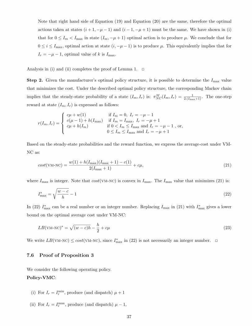
Note that right hand side of Equation (19) and Equation (20) are the same, therefore the optimal
actions taken at states (i + 1,−µ− 1) and (i− 1,−µ + 1) must be the same. We have shown in (i)
that for 0 ≤ Im < Imax in state (Im,−µ + 1) optimal action is to produce µ. We conclude that for
0 ≤ i ≤ Imax, optimal action at state (i,−µ− 1) is to produce µ. This equivalently implies that for
Ir = −µ − 1, optimal value of k is Imax.
Analysis in (i) and (ii) completes the proof of Lemma 1.
Step 2. Given the manufacturer’s optimal policy structure, it is possible to determine the Imax value
that minimizes the cost. Under the described optimal policy structure, the corresponding Markov chain
implies that the steady-state probability of a state (Im, Ir) is: πMNC(Im, Ir) = 1
2.(Imax+1) . The one-step
reward at state (Im, Ir) is expressed as follows:
r(Im, Ir) =
cµ + w(1) if Im = 0, Ir = −µ − 1c(µ − 1) + h(Imax) if Im = Imax, Ir = −µ + 1cµ + h(Im) if 0 < Im ≤ Imax and Ir = −µ − 1 , or,
0 ≤ Im ≤ Imax and Ir = −µ + 1
Based on the steady-state probabilities and the reward function, we express the average-cost under VM-
NC as:
cost(vm-nc) =w(1) + h(Imax)(Imax + 1) − c(1)
2(Imax + 1)+ cµ, (21)
where Imax is integer. Note that cost(vm-nc) is convex in Imax. The Imax value that minimizes (21) is:
I∗max =
√
w − c
h− 1 (22)
In (22) I∗max can be a real number or an integer number. Replacing Imax in (21) with I∗max gives a lower
bound on the optimal average cost under VM-NC:
LB(vm-nc)∗ =√
(w − c)h −h
2+ cµ (23)
We write LB(vm-nc) ≤ cost(vm-nc), since I∗max in (22) is not necessarily an integer number.
7.6 Proof of Proposition 3
We consider the following operating policy.
Policy-VMC:
(i) For Ir = Iminr , produce (and dispatch) µ + 1
(ii) For Ir = Imaxr , produce (and dispatch) µ − 1,
37

(iii) Otherwise, for Iminr < Ir < Imax
r , produce (and dispatch) µ,
where we assume Imaxr ≥ Imin
r +3 (i.e., under Policy-VMC there exist at least four states). The proposed
policy, Policy-VMC, is not necessarily the optimal policy under VM-C, therefore the cost implied by
this policy will be an upper bound on the optimal cost under VM-C. Note that the transition probabilities
for all Ir are 12 . The transition diagram of the underlying Markov chain is presented in Figure 7.
Irmin ..............Irmin +1 Irmin +2 IrmaxIrmax-1Irmax-2
1/2
1/2
1/2 1/2
1/2 1/21/2
1/2
1/2
Figure 7: The transition diagram of the underlying Markov chain under Policy-VMC under VM-C.
The steady-state probabilities, πMC (Ir), implied by Policy-VMC are as follows:
πMC (Ir) =
12∆ for Ir = Imin
r , Iminr + 1, Imax
r − 1, Imaxr
1∆ for Imin
r + 1 < Ir < Imaxr − 1
0 o/w
where ∆ = Imaxr − Imin
r − 1. The reward in state Ir is expressed as follows:
r(Ir) =
cµ + w(1) if Ir = Iminr
c(µ − 1) + h(Imaxr ) if Ir = Imax
r
cµ + h(Ir)+ Imin
r < Ir < Imaxr
(24)
Our aim is to determine an upper bound on the optimal average cost under VM-C. Note that in (24),
Imaxr is always positive, since otherwise β ≥ 1. Furthermore, Imin
r is non-positive (since it is already
possible to attain 100% when Iminr = 0). When determining Imin
r and ∆ we make sure that the service
level constraint in (13), where β ∈ S, is satisfied. In other words the following constraint is satisfied:∑i=0
i=Iminr
|i|πMC (Ir = i)
E[D]≤ β (25)
Based on r(Ir) and πMC (Ir) we write an upper bound on optimal average cost, UB(vm-c), as follows:
UB(vm-c) = r(Ir)πMC (Ir) = w
1
2∆+ h(
1
∆+
2
∆+ · · · +
Imaxr − 2
∆+
Imaxr − 1
2∆+
Imaxr
2∆) − c
1
2∆+ cµ.
The cost, UB(vm-c), consists of the cost of production and outsourcing in all states {Iminr , · · · , Imax
r }
and the cost of holding inventory in states {1, 2, · · · , Imaxr }. Replacing Imax
r with ∆ − |Iminr | + 1:
UB(vm-c) = w1
2∆+ h(
1
∆+
2
∆+ · · ·+
∆ − |Iminr | − 1
∆+
∆ − |Iminr |
2∆+
∆ − |Iminr | + 1
2∆)− c
1
2∆+ cµ,
which is equivalent to,
UB(vm-c) =
h(∆−|Iminr |+1/2)2+w−c+ 3
4h
2∆ + cµ if Imaxr ≥ 3
w 12∆ + h(1
2∆ + 22∆) − c 1
2∆ + cµ if Imaxr = 2
w 12∆ + h(1
2∆) − c 12∆ + cµ if Imax
r = 1
(26)
To make the analysis simpler we focus on the case where Imaxr ≥ 3. This is equivalent to ∆ − |Imin
r | ≥ 2.
In summary we make the following assumptions when defining Policy-VMC.
38

A1. Iminr ≤ 0,
A2. ∆ − |Iminr | ≥ 2
From second order condition, for Imaxr ≥ 3 the expression in (26) is convex in ∆. From the first order
condition, the minimizing ∆ is obtained as a function of Iminr as follows:
∆∗ =
√
w − c
h+ (|Imin
r |2 − |Iminr | + 1)
In order to obtain a “reasonable” upper bound (i.e., an upper bound which is not very relaxed), we
consider the ∆ that minimizes (26). To determine the values Iminr could take, we make the following
observation. Observation. Production and outsourcing cost of the manufacturer is independent of Iminr ,
and the inventory holding cost decreases as Iminr decreases.
The observation implies that for a given ∆, as Iminr decreases total cost decreases. If there were no service
level constraint, to lower the cost one should lower the Iminr value. However, there is a limit on the lowest
value Iminr can take when minimizing UB(vm-c), determined by the service level. Based on (25) and
considering Imaxr ≥ 3:
|Iminr |
2∆+
|Iminr | − 1
2∆+
|Iminr | − 2
∆+ · · · +
1
∆≤ βµ.
In the expression above, for β = 0 (i.e, for 100% service level) Iminr should be 0. Otherwise, to be able to
set |Iminr | as high as k, β should satisfy:
β ≥k2 − k + 1
2µ∆for k = 1, · · · (27)
For a required service level, if the |Iminr | level is set to its highest possible value, then this would correspond
to the lowest possible inventory holding cost under that service level. A limit on how high |Iminr | can
be set is obtained from Equation (27). For a given |Iminr |, ∆∗ minimizes the UB(vm-c) value. We place
∆∗ in equation (27) and we suggest two possible upper bound values for optimal average cost under
VM-C: UB1 for Iminr = 0, and a generalized upper bound for |Imin
r | > 0.
Upper bound 1 (UB1). We set Iminr to the highest possible value, Imin
r = 0. Since as Iminr decreases,
UB(VM-C) decreases, upper bound obtained under Iminr = 0 can be regarded as a “relaxed” upper
bound.
For Iminr = 0, we obtain ∆∗ =
√
w−ch + 1. From Assumption A2, ∆∗ must be greater than or equal to
2. This is equivalent to, w ≥ 3h + c. Furthermore to guarantee that the expression in (26) is an upper
bound, ∆∗ must be an integer. Equivalently, we say, w should be such that ∆∗ is integer-valued.
Placing Iminr = 0 and ∆∗ in (26) we obtain the following.
39

Suppose that w ∈ W, where W = {w|w ≥ 3h+c,√
w−ch + 1 ∈ Z
+}. Then UB(VM-C) = h(√
w−ch + 1+
12) + cµ is an upper bound on the optimal average cost under VM-C.
A generalized upper bound. We construct a more general set of conditions for determining an upper
bound. Let Iminr = k. For Imin
r = k, we obtain ∆∗ =√
w−ch + (|Imin
r |2 − |Iminr | + 1). From Assumption
A2, ∆∗ must be greater than or equal to |Iminr | + 2. This is equivalent to, w ≥ (5|Imin
r | + 3)h + c. Also,
∆∗ must be an integer.
For a required service level 1 − β, highest |Iminr | level is obtained as follows:
1 − β ≤ 1 −|Imin
r |2 − |Iminr | + 1
2µ√
w−ch + |Imin
r |2 − |Iminr | + 1
(28)
Placing Iminr and ∆∗ in (26) we obtain the following.
Suppose that w ∈ W, where W = {w|w ≥ (5k + 3)h + c,√
w−ch + (k2 − k + 1) ∈ Z
+} and SL ≤
1 − k2−k+1
2µq
w−c
h+k2−k+1
. Then UB(VM-C) = h(√
w−ch + k2 − k + 1 − (k − 1
2)) + cµ, where k ∈ Z+, is an
upper bound on the optimal average cost under VM-C.
7.7 Proof of Proposition 4
We compare LB(VM-NC)and UB(VM-C) and obtain the (sufficient) conditions under which VM-NC
results in higher cost than VM-C. In Proposition 3 we obtain two upper bounds for the optimal average
cost of VM-C.
First we compare UB1 with LB(VM-NC). UB1 may be a reasonable upper bound when the service level
requirement is very high. When Iminr = 0, upper bound is expressed as: UB(VM-C) = h(
√
w−ch + 1 +
12)+cµ. Comparing this with LB(VM-NC) =
√
(w − c)h− h2 +cµ, we obtain that UB(VM-C) is always
higher than the LB(VM-NC). Similarly, when Iminr = 1, we again obtain that UB(VM-C) is higher
than the LB(VM-NC). Therefore we conclude that when service level requirement at the retailer is high,
it is less likely that VM-C results in lower cost.
For Iminr ≥ 2, under ∆∗ the upper bound in (26) is expressed as:
UB(VM-C) = h(√
w−ch + |Imin
r |2 − |Iminr | + 1) − (|Imin
r | − 12)) + cµ.
Comparing this with LB(VM-NC), we obtain the following:
UB(VM-C) < LB(VMNC)
h(√
w−ch + (|Imin
r |2 − |Iminr | + 1) − (|Imin
r | − 12)) < h(
√
w−ch − 1
2)
|Iminr | < 2
√
w−ch (|Imin
r | − 1)
40

As |Iminr | increases it is more likely that VM-C yields lower cost. For Imin
r = k, w > 14( k
k−1)2h + c
is a sufficient condition for UB(VM-C) < LB(VM-NC). Note that, in Proposition 3 we obtained
w ≥ (5k + 3)h + c, for k ≥ 1 as a tighter condition than w > 14( k
k−1)2h + c. Therefore we only consider
w ≥ (5k + 3)h + c.
We summarize the sufficient conditions for preferring VM-C over VM-NC as follows:
1. SL ≤ 1 − k2−k+1
2µq
w−c
h+k2−k+1
2. w ≥ (5k + 3)h + c
3. w is such that√
w−ch + k2 − k + 1 is integer-valued.
4. k ≥ 2
We conclude that when the sufficient conditions are satisfied, the optimal cost under VM-C is lower than
the optimal cost under VM-NC.
References
Aviv, Y. and Federgruen, A. (1997). Stochastic Inventory Models with Limited Production Capacity and
Periodically Varying Parameters. Probability in Engineering and Informational Sciences, 11, 107–135.
Aviv, Y. and Federgruen, A. (1998). The Operational Benefits of Information Sharing and Vendor
Managed Inventory (VMI) Programs. Unpublished Manuscript.
Barnes, E., Dai, J., Deng, S., Down, D., Goh, M., H., C. L. and Sharafali, M. (2000). On the Strategy of
Supply Hubs for Cost reduction and Responsiveness. White Paper, School of Industrial and Systems
Engineering, Georgia Institute of Technology, Atlanta, Georgia, USA.
Bernstein, F., Chen, F. and Federgruen, A. (2006). Coordinating Supply Chains with Simple Pricing
Schemes: The Role of Vendor Managed Inventories. Management Science, 52, 1483–1492.
Cachon, G. and Fisher, M. (1997). Campbell Soup’s Continuous Replenishment Program: Evaluation
and Enhanced Inventory Decision Rules. Production and Operations Management , 6, 266–276.
Cetinkaya, S. and Lee, C. Y. (2000). Stock Replenishment and Shipment Scheduling for Vendor-Managed
Inventory Systems. Management Science, 46, 217–232.
Choi, K. S., Dai, J. G. and Song, J. S. (2004). On Measuring Supplier Performance Under Vendor-
Managed-Inventory Programs in Capacitated Supply Chains. Manufacturing and Service Operations
Management , 6, 53–72.
41

Disney, S. and Towill, D. (2003). The Effect of Vendor Managed Inventory (VMI) Dynamics on the
Bullwhip Effect in Supply Chains. International Journal of Production Economics, 85, 199–215.
Dong, Y. and Xu, K. (2002). A Supply Chain Model of Vendor Managed Inventory. Transportation
Research Part E , 38, 75–95.
Fishman, C. (2006). The Wal-Mart Effect. Publisher: Marti Kitabevi, Turkey.
Fry, M. J., Kapuscinski, R. and Olsen, T. L. (2001). Coordinating Production and Delivery Under a
(z,Z)-Type Vendor-Managed Inventory Contract. Manufacturing and Service Operations Management ,
3, 151–173.
Gavirneni, S., Kapuscinski, R. and Tayur, S. (1999). Value of Information in Capacitated Supply Chains.
Management Science, 45, 16–22.
Hausman, W. (2003). Supplier Managed Availability. http://www.supplychainonline.com.
Jaruphongsa, W., Cetinkaya, S. and Lee, C. Y. (2004). Warehouse Capacity and Delivery Time Window
Considerations in Dynamic Lot-Sizing for a Simple Supply Chain. International Journal of Production
Economics, 92, 169–180.
Kahn, G. (2002). Made to Measure: Invisible Supplier Has Penney’s Shirts All Buttoned Up. The Wall
Street Journal , Sept. 11.
Kapuscinski, R. and Tayur, S. (1998). A Capacitated Production-Inventory Model with Periodic Demand.
Operations Research, 46, 899–911.
Kleywegt, A. J., Nori, V. S. and Savelsberg, M. W. P. (2002). The Stochastic Inventory Routing Problem
with Direct Deliveries. Transportation Science, 36, 94–118.
Lee, H. L., Padmanabhan, V. and Whang, S. (1997). Information Distortion in a Supply Chain: The
Bullwhip Effect. Management Science, 43, 546–558.
Li, X. and Wang, Q. (2007). Coordination Mechanisms of Supply Chain Systems. European Journal of
Operational Research, 179, 1–16.
Maxwell, W. L. and Muckstadt, J. A. (1985). Establishing Consistent and Realistic Reorder Intervals in
Production-Distribution Systems. Operations Research, 33, 1316–1341.
Nagarajan, M. and Rajagopalan, S. (2008). Contracting under Vendor Managed Inventory Systems Using
Holding Cost Subsidies. Production and Operations Management , 17, 200–210.
Nelson, E. and Zimmerman, A. (2000). Minding the Store: Kimberly-Clark Keeps Costco in Diapers,
Absorbing Costs Itself. The Wall Street Journal , Sept. 07.
42

Puterman, M. L. (1994). Markov Decision Processes: Discrete Stochastic Dynamic Programming. John
Wiley and Sons, New York.
Schenck, J. and McInerney, J. (1998). Applying Vendor-Managed Inventory to the Apparel Industry.
Automatic I.D. News, 14, 36–38.
Shah, J. and Goh, M. (2006). Setting Operating Policies for Supply Hubs. International Journal of
Production Economics, 100, 239–252.
Valentini, G. and Zavanella, L. (2003). The Consignment Stock of Inventories: Industrial Case and
Performance Analysis. International Journal of Production Economics, 81-82, 215–224.
Veinott, A. F. (1965). The Optimal Inventory Policy for Batch Ordering. Operations Research, 13, 424–
432.
Waller, M., Johnson, M. E. and Davis, T. (1999). Vendor-managed Inventory in the Retail Supply Chain.
Journal of Business Logistics, 20, 183–203.
Zheng, Y. and Chen, F. (1992). Inventory Policies with Quantized Ordering. Naval Research Logistics,
39, 285–305.
43