An aggregate model for transient andmulti-directional pedestrian flows in public

walking areas

Flurin S. Hänseler∗ Michel Bierlaire∗ Bilal Farooq†

Thomas Mühlematter∗

December 19, 2013

Report TRANSP-OR 131219Transport and Mobility Laboratory

School of Architecture, Civil and Environmental EngineeringEcole Polytechnique Fédérale de Lausanne

transp-or.epfl.ch

∗École Polytechnique Fédérale de Lausanne (EPFL), School of Architecture, Civil andEnvironmental Engineering (ENAC), Transport and Mobility Laboratory, Switzerland,{flurin.haenseler,michel.bierlaire,thomas.muhlematter}@epfl.ch

†Département des Génies Civil, Géologique et des Mines, Polytechnique Montréal,Canada, bilal.farooq@polymtl.ca

1

Abstract

A dynamic pedestrian propagation model applicable to congested and multi-directional flows is proposed. Based on the cell transmission model, severalimportant extensions are made to describe the simultaneous and poten-tially conflicting propagation of multiple pedestrian groups. Their move-ment across space and time can be individually tracked, such that group-specific travel time distributions can be predicted. Cell potentials allow foren-route path choice that takes into account prevailing traffic conditions.The model is formulated at the aggregate level and thus computationallycheap, which is advantageous for studying large-scale problems. A de-tailed analysis of several basic flow patterns including counter- and crossflows, as well as two generic scenarios involving a corner- and a bottle-neck flow is carried out. Depending on the choice of model parameters,various behavioral patterns ranging from disciplined queueing to impatientjostling can be realistically reproduced. Following a systematic model cal-ibration using real data, an extensive case study involving a Swiss rail-way station is presented. A comparison with the social force model andpedestrian tracking data shows a good performance of the proposed modelwith respect to predictions of travel times and pedestrian density fields.

Keywords: Pedestrian propagation, cell-transmission model, multi-directionalflow, en-route path choice, calibration.

1

1 Introduction

In railway stations and other public spaces, pedestrian flows are often multi-directional, non-stationary and congested (Daamen, 2004). To gain a betterunderstanding of such flows, there is a general need for adequate, quanti-tative models that can predict pedestrian movements and travel times fora given infrastructure and demand.

A central challenge in pedestrian flow modeling consists in predictinglevel of service (LOS) of walking facilities. From a modeling point of view,LOS assessment requires the assignment of pedestrian demand to the in-frastructure and the computation of resulting flows. In this process, thenumber of pedestrians traveling between each origin-destination pair needsto be known a priori. Local flows are calculated by a pedestrian propaga-tion model, from which various LOS indicators can be extracted. A typicalLOS indicator is for instance pedestrian density, which is considered animportant factor for safety and customer satisfaction.

A recent review of pedestrian propagation models has been carried outby Duives et al. (2013), who provide a broad overview of modeling achieve-ments in the last two decades. Their study covers in particular the socialforce model (Helbing and Molnár, 1995), cellular automata (Blue and Adler,2001), queueing networks (Løvås, 1994), behavioral models (Robin et al.,2009), activity choice models (Hoogendoorn and Bovy, 2004), continuummodels (Hughes, 2002) and two further models that are associated with thegaming industry. These models are compared and evaluated with respectto three criteria. First, their ability to reproduce basic movement patternssuch as a bottleneck- or a bi-directional flow is assessed. Second, their ca-pabilities to describe self-organization phenomena such as lane formationor stop-and-go waves is examined. Third, practical considerations such ascomputational cost and general applicability are investigated.

One of the conclusions of their study is that current models can bedivided into slow but precise microscopic approaches and fast but behav-iorally questionable macroscopic modeling attempts. It is argued that forcrowd simulation models to be used in practice, the identified gap needsto be closed. This is where the present study would like to make a contri-bution. Our approach does not fit in any of the model categories listed byDuives et al. (2013). It is designed such that it is not only useful for infras-tructure assessment, but also helpful in the inverse problem of estimating

2

pedestrian demand.In transportation hubs, pedestrian demand changes rapidly and may

fluctuate by several orders of magnitude over a day. Both the total num-ber of pedestrian trips per time and the corresponding route fractions maycontinuously change. A precise demand estimation requires thus the com-bination of several information sources such as pedestrian flow counters,pedestrian tracking systems or sales data from service points and ticketvending machines. To associate sensor data obtained at different locationsover space and time, it is crucial to have an accurate estimate of walkingtimes.

The above modeling problems – infrastructure assessment, flow assign-ment, demand estimation – are closely interwoven. Flow propagation de-pends on demand. Inversely, demand estimation relies on travel time pre-dictions provided by a pedestrian propagation model. In this work, wefocus on a flow propagation model, but keep these interdependencies inmind. Specifically, we aim at developing a pedestrian propagation modelthat can accurately predict travel time distributions, flows and pedestriandensities, and is versatile enough to interact with a demand estimation andan assignment model.

For this purpose, we propose the use of an aggregate pedestrian flowmodel due to several reasons: First, aggregate models are computation-ally cheap and can therefore be readily integrated in a dynamic pedestriantraffic assignment model (in the context of car traffic e.g. Ben-Akiva et al.,2001; Mahmassani, 2001; Abdelghany et al., 2012). Such a joint demand es-timation/flow assignment approach typically requires solving a fixed point(see Bierlaire and Crittin, 2006; Cascetta and Postorino, 2001, for relatedexamples). This makes multiple runs of the pedestrian propagation modelnecessary, amplifying the performance difference between aggregate anddisaggregate models. In such a context, the use of disaggregate modelsfor large problems would quickly become infeasible. Second, the problemof origin-destination demand estimation is often considered at the aggre-gate level (again examples from car traffic: Cascetta et al., 1993; Ashokand Ben-Akiva, 2000; Sherali and Park, 2001). In this case, an assignmentmodel operating at the same level of aggregation allows for direct inter-action with the demand estimation methodology without prior populationsynthesis, which is computationally advantageous. Third, calibration ofmacroscopic models is relatively easy (Hoogendoorn and Bovy, 2001). In

3

contrast, calibration of microscopic models is challenging due to variousreasons. Often a lack of disaggregate data necessitates a calibration basedon a comparison of macroscopic outcomes of the model. Such an approachis unlikely to produce the optimal parameters since the number of degreesof freedom is too large. It is not guaranteed that the obtained specificationis able to describe individual behavior accurately, or if it merely provides areasonable average macroscopic prediction for the situation it is calibratedfor (Hoogendoorn and Daamen, 2007). If disaggregate data is available,calibration still remains difficult. For the widely used social force model,microscopic calibration has been achieved only for a controlled bottleneckflow (Hoogendoorn and Daamen, 2007), or by neglecting inter-pedestrianvariability (Johansson et al., 2007).

In the following, we first give an overview of existing aggregate pedes-trian propagation models. We then outline a new model, explicitly de-signed for dynamic, multi-directional and congested pedestrian flow prob-lems. Subsequently, this model is calibrated on real data, analyzed in detailusing various test cases, and applied to a case study.

2 Aggregate pedestrian flow models

In the literature, three types of aggregate pedestrian propagation modelshave been considered: (i) Models based on continuum theory for pedestrianflows, (ii) queueing network based models (QNM), and (iii) cell transmis-sion models (CTM).

The first type is aggregate with respect to agents, and operates in con-tinuous space. The second type considers pedestrians at the disaggregatelevel, relying on a graph-based space representation. The third model typeis aggregate both with respect to space and pedestrians, i.e., space is ‘ag-gregated’ to a network, and pedestrians are subsumed as groups.

Continuum theory for pedestrians is formulated as a set of partial differ-ential equations, in which the direction of flow is defined by one or severalcontinuous potential fields (Hughes, 2002). It is mostly used for evacuationsimulations, where only a small number of origin-destination flows need tobe considered.

QNM is based on random queueing processes and can be either ap-proximated analytically for stationary problems (Cheah and Smith, 1994;

4

Osorio and Bierlaire, 2009), or by simulation (Løvås, 1994; Daamen, 2004;Rahman et al., 2013). Propagation of agents along their route is describedat the disaggregate level. Due to the microscopic nature of QNM, it isstraightforward to consider agent-specific routes. In the context of car traf-fic, Çetın (2005) reports that an accurate modeling of backward travelingjam waves using QNM is difficult. Guaranteeing a fair behavior in ‘inter-sections’ seems possible, but is far from trivial (Charypar, 2008, again inthe context of car traffic).

CTM represents a finite difference approximation to first-order flow the-ory (Daganzo, 1994, 1995). Like the continuum theory for pedestrians, itrepresents a deterministic approach and is of aggregate nature, which makesit computationally cheap. For prediction of flows, CTM relies on a funda-mental diagram relating density and speed.

A few studies consider CTM or derived concepts to study pedestrianflows. Al-Gadhi and Mahmassani (1991) developed a cell-based pedestrianwalking model with application to the circular movements around stonemonuments occurring during the Hajj, a Muslim pilgrimage to Makkah,Saudi Arabia. The model consists of a set of coupled differential equationsincluding a flow conservation equation that is solved numerically. A speed-density relationship is considered to describe the multidirectional move-ment. Their work can be seen as an early prototype of the CTM introducedlater by Daganzo. Asano et al. (2007) extended CTM to describe generalmulti-directional pedestrian flows, assuming a trapezoidal fundamental di-agram inherited from the original CTM. Their model is applicable to caseswhere the exact sequence of cells that a pedestrian traverses is known inadvance. They illustrate the model using a generic cross-flow problem. Guoet al. (2011) developed a cell-based model for describing evacuation pro-cesses. Instead of relying on a density-flow relationship, they assume thatthe number of pedestrians exchanged between adjacent cells depends onthe ‘opening’ between them. The size of this opening is given exogenously,which represents a major simplification with respect to the original CTM.Flows between cells are computed based on cell potentials, cell capacityconstraints and the previously mentioned openings. Besides the cell-basedspace representation, their model is not directly related to Daganzo’s CTMand hardly applicable to other problems than evacuation.

In this study, we develop an aggregate pedestrian propagation modelbased on the original CTM and the above mentioned derived models.

5

Thanks to the use of an empirical fundamental diagram for pedestrianflows, it can realistically reproduce pedestrian flow patterns under manyconditions. In particular, this includes pedestrian waves, which often occurin transportation hubs after the arrival of mass transport vehicles such astrains. We build on the framework for multi-directional flows proposed byAsano et al. (2007) and adapt the concept of cell-specific potentials pro-posed by Guo et al. (2011). This approach allows for en-route path choice,making an exogenous definition of exact cell sequences for pedestrians need-less. The resulting model can accurately describe everyday pedestrian flowsin public walking areas and is performant thanks to its aggregate nature.

3 A cell-based pedestrian flow model

The cell transmission model considers time in discrete space, i.e., the pe-riod of analysis is discretized into a set of intervals T , where each intervalτ = 1, . . . , T is of uniform length ∆t. Similarly, space is discretized intosquare cells ξ of characteristic length ∆L as shown in figure 1. In principle,triangular or hexagonal grids are possible as well, but most practical lay-outs can be represented more realistically with a square grid that inherentlyallows for orthogonal movements.

The cell network is represented by a directed graph G = (X ,Y), whereX represents the set of cells ξ and Y the set of links ξ → ξ ′ connectingthem. Each cell has an individual area Aξ, which may deviate from thedefault size ∆L2 in presence of obstacles. Such obstacles include any objectthat reduces the walkable space in a cell but is small in comparison, suchas e.g. a pillar or a trash bin. Adjacent cells are connected to each otherif they share a cell edge. The set of neighbors of a cell ξ is denoted byNξ. Pedestrian flows from one cell to another are governed by the flowpropagation model described in the following.

The central idea of the cell transmission model is to formulate a con-servation principle with respect to the number of pedestrians in each celland to combine it with a fundamental diagram for calculating the flows be-tween them. Within a cell, pedestrians are assumed to be homogeneouslydistributed, and their movements are not modeled explicitly.

To estimate the walking speed of pedestrians, an empirical density-speedrelation is employed. Let k denote the space-mean density, i.e., the number

6

Entrance

Railway line/platform

Figure 1: Space is discretized into a number of cells (delimited by dotted lines).Contiguous sets of cells represent areas (delimited by dashed lines). Each pedes-trian is assigned to a sequence of these areas, which is referred to as a route(example shown in red).

of pedestrians per unit space, and let v be the space-mean speed, defined asthe average speed of pedestrians per unit space. According to Weidmann(1993), the velocity of pedestrians in public spaces depends on density asfollows (figure 2)

v(k) = vf

{1− exp

[

−γ

(

1

k−

1

kc

)]}, 0 ≤ k ≤ kc, (1)

where vf denotes free-flow speed (1.34 m/s according to Weidmann, 1993),γ is a shape parameter (1.913 m−2), and kc represents jam density (5.4 m−2).Being one of the most widely used empirical fundamental diagrams, we uti-lize it in this work as well. Generalizations to other fundamental diagramsturn out to be straightforward. Common to all of them is that they do notconsider speed as a vector, but as a scalar representing some average value.An overview of existing pedestrian fundamental diagrams is provided e.g.by Seyfried et al. (2005).

To guarantee the equivalence between CTM and kinematic wave theory,the time step ∆t has to be chosen in agreement with the free-flow speed vfand the cell length ∆L. Specifically, the following relation has to be fulfilled

vf∆t = ∆L, (2)

7

0

0.5

1

1.34

1.5

v(m

/s)

0 1 1.75 3 4 5 5.4 60

0.5

1

1.22

1.5

k (m−2)

q(m

−1s−

1)

Figure 2: Pedestrian space-mean speed (solid blue) and specific hydrodynamicflow (dashed red) as a function of density according to Weidmann (1993).

which implies that under free-flow conditions, pedestrians propagate fromone cell to the next during one time step. A derivation of this condition isprovided by Daganzo (1994).

For pedestrians within a given cell, the edge through which they en-ter and leave the cell are known. We assume that they cross these edgesorthogonally. The sum of all pedestrians in the cell, N = k∆L2, can be at-tributed to the contributions of each pair of inflow and outflow edge {i, j},Ni,j, such that N =

∑4i=1

∑4j=1 Ni,j.

The cumulated outflow across edge j ∈ {1, 2, 3, 4} during an infinitesimaltime interval dt associated with the fundamental diagram is then equal tothe number of pedestrians in an infinitesimal area of size ∆Lv(k)dt that areheaded to edge j, i.e.,

dQoutj = ∆Lv(k)dt

4∑

i=1

Ni,j

∆L2, (3)

where the unit is number of pedestrians. By taking the sum over all edges,the cumulated outflow from a cell during an infinitesimal time interval dt

8

associated with the fundamental diagram is given by

dQouttot = ∆Lv(k)dt

4∑

i=1

4∑

j=1

Ni,j

∆L2= ∆Lv(k)dtk. (4)

Dividing by the cell length ∆L and the infinitesimal time interval dt, thespecific outflow from a cell associated with the fundamental diagram canbe obtained (figure 2)

qh(k) = v(k)k. (5)

Equation 5 is referred to as hydrodynamic flow-density relation in the lit-erature (see e.g. Kesting, 2012, for an example in the context of multi-lanecar traffic). The quantity qh, which is a function of the overall density k

only, is accordingly referred to as hydrodynamic flow.Previously, qh(k) has been derived based on the outflow from a cell.

The same expression results if the derivation is based on the inflow. Thehydrodynamic flow qh(k) represents a characteristic flow per unit time andunit length that is associated with the density-speed relation (1). Since itonly considers the density of a single cell, and since it does not take intoaccount any capacity constraints that will be discussed in the following, itdoes not represent an actual flow.

Let us now introduce a concept allowing to describe how pedestriansinteract with their environment. We assume that there exists a finite set ofroutes R along which pedestrians can walk. Intuitively, a route ρ ∈ R canbe thought of as a sequence of areas without loops, ρ = (rρo, r

ρ1, r

ρ2, . . . , r

ρd),

such as ‘entrance north, train station hall, pedestrian underpass west, plat-form #3’. Each of these areas r represents a non-empty subgraph of G.The first and the last area, ro and rd, consist of exactly one cell. Theseboundary cells can be adjacent to an arbitrary number of cells and are notsubject to any capacity constraints. While their typical position is at theborder of a walking area, boundary cells can also be located in the interiorif they represent an access way to e.g. an elevator or an escalator. Therecan be several routes connecting the same pair of boundary cells. Eachroute starts and ends at a boundary cell, but cannot contain a boundarycell in between.

Pedestrian demand along a route ρ ∈ R emanating during time intervalτ is denoted by Xρ,τ. A pedestrian group ℓ is defined by a route ρℓ anda departure time interval τℓ. Group size Xρ,τ is its main characteristic.

9

Several groups can share the same route ρ if they are assigned to a differentdeparture time interval and vice versa. The set of all pedestrian groups isdenoted by L ⊂ R×T . In this work, we assume that the pedestrian routedemand X = [Xρ,τ] is known a priori.

To apply the density-speed relation (1) to a cell, we need to know itsoccupation. The total population in cell ξ during time interval τ is givenby

M(ξ, τ) =∑

ℓ∈L

Mℓ(ξ, τ) (6)

where Mℓ(ξ, τ) represents the number of people in cell ξ during interval τthat belong to group ℓ. The cumulated hydrodynamic flow of cell ξ dur-ing time interval τ, formally defined as the integral of hydrodynamic flow(equation 5) over the interval τ and the circumference of cell ξ, reads forWeidmann’s fundamental diagram (equation 1) as

Qξ(τ) = M(ξ, τ)

{1− exp

[

−γAξ

(

1

M(ξ, τ)−

1

Nξ

)]}(7)

where Nξ = kcAξ denotes the maximum number of people that can becontained by cell ξ at jam density kc. The cumulated hydrodynamic cellflow reaches a cell-specific optimum Qξ,opt at occupation Mξ,opt, similar tothe hydrodynamic flow shown in figure 2. Two quantities are derived fromit: The hydrodynamic outflow capacity denotes the maximum number ofpedestrians that can leave cell ξ during time interval τ according to thefundamental diagram, and is given by

Q̃ξ(τ) =

{Qξ(τ) if M(ξ, τ) ≤ Mξ,opt,

Qξ,opt otherwise.(8)

Similarly, the hydrodynamic inflow capacity represents the maximum num-ber of people that can enter cell ξ during time interval τ according to thefundamental diagram and is defined as

Q̂ξ(τ) =

{Qξ,opt if M(ξ, τ) ≤ Mξ,opt,

Qξ(τ) otherwise.(9)

For en-route path choice, a static floor field Fρξ and a dynamic floor fieldHξ(τ) are introduced. The route-specific static floor field Fρξ represents theremaining distance from cell ξ along route ρ, i.e., the minimum number

10

of cells to be traversed from cell ξ to the end of route ρ along route ρ. Itcan be calculated using any shortest path algorithm (e.g. Dijkstra, 1959).The dynamic floor field Hξ(τ) is assumed to be equal to the prevailingnormalized walking speed v (M(ξ, τ)/Aξ) /vf. The rationale behind thischoice is that pedestrians are expected to give preference to cells in whichthey can walk at free-flow speed, similar to the concept of the desiredvelocity in the social force model (Helbing and Molnár, 1995).

Based on these floor fields, each cell is assigned a route-specific, density-dependent potential

Pρξ(τ) = αFρξ − βHξ(τ) (10)

where the parameters α, β ∈ R+ denote weights that can assume any posi-

tive value and do not need to sum up to unity. Both floor fields as well asthe corresponding weights are non-dimensional.

From the cell potentials, turning proportions for local path choice canbe calculated. Pedestrians can only be sent to adjacent cells that are partof their route. The set Θρ

ξ contains all cells which are adjacent to cell ξ

and part of route ρ. Assuming that all pedestrians embarked on a givenroute have the same behavior, the turning proportion corresponding to linkξ → ϑ ∈ Θρ

ξ for the ensemble of people following route ρ that are in cell ξduring time interval τ can be expressed as

δρξ→ϑ(τ) =exp

{Pρξ(τ) − Pρ

ϑ(τ)}

∑ϑ ′∈Θ

ρ

ξexp

{Pρξ(τ) − Pρ

ϑ ′(τ)} . (11)

Expression 11 is consistent with the discrete choice theory (Ben-Akiva andLerman, 1985), according to which it represents the probability of a singleagent in cell ξ embarked on route ρ to be headed to cell ϑ ∈ Θρ

ξ duringtime interval τ. Due to the assumption of a homogeneous population, it alsorepresents the turning proportion of the ensemble of pedestrians travelingon the same route. The use of a more advanced model (?Robin et al.,2009) could be considered. However, there is a trade-off between behavioralrealism and computational performance which should be assessed first.

The combination of equations (10) and (11) provides a behavioral inter-pretation of the weights α and β. A large value of α means that pedestriansfollow the shortest path corresponding to their route very closely. Analog-ically, a high value of β implies that pedestrians prefer less busy cells inwhich they can walk as fast as possible.

11

As in the original cell transmission model proposed by Daganzo (1995),a sending and receiving capacity is defined for each cell, representing themaximum number of pedestrians who can leave and enter a cell, respec-tively.

The sending capacity of cell ξ to cell ϑ ∈ Θρξ for group ℓ during time

interval τ is given by

Sℓξ→ϑ(τ) = δρℓξ→ϑ(τ)min

{Mℓ(ξ, τ),

Mℓ(ξ, τ)

M(ξ, τ)Q̃ξ(τ)

}. (12)

Under non-congested conditions, all pedestrians advance to the next cell(first term in curly brackets). In the presence of congestion, i.e., if the sumof pedestrians in cell ξ is superior to the hydrodynamic outflow capacityQ̃ξ(τ), the latter is assigned to all groups present in cell ξ according to ademand-proportional supply distribution scheme (Asano et al., 2007).

The counterpart of the sending capacity is the receiving capacity. Forcell ξ and time interval τ, it can be expressed as

Rξ(τ) = min{Nξ −M(ξ, τ), Q̂ξ(τ)

}(13)

where the first term in brackets represents the number of pedestrians forwhich space is left in the cell, and the second term represents the hydro-dynamic inflow capacity.

The actual flow of people belonging to group ℓ from cell ξ to an adjacentcell ϑ ∈ Θρℓ

ξ during time interval τ can be expressed as

Yℓξ→ϑ(τ) =

{Sℓξ→ϑ(τ) if

∑ν∈Nϑ

∑ℓ∈L S

ℓν→ϑ(τ) ≤ Rϑ(τ),

ζℓξ→ϑ(τ)Rϑ(τ) otherwise.(14)

In the presence of congestion, i.e., if the sum of sending capacities allocatedto a cell exceeds the receiving capacity of that cell, it is allocated propor-tionally to the various inflowing groups (Asano et al., 2007). The supplydistribution scheme for the receiving capacity is then given by

ζℓξ→ϑ(τ) =Sℓξ→ϑ(τ)∑

ν∈Nϑ

∑ℓ∈L S

ℓν→ϑ(τ)

. (15)

Note that flows to cells which are not adjacent with respect to the route ofinterest are always zero, i.e., Yℓ

ξ→ϑ ′(τ) = 0 if ϑ ′ /∈ Θρℓξ .

12

For boundary cells, an exogenous generation term Wℓ(ξ, τ) adds outgo-ing groups at their origin during the foreseen departure time interval, andremoves incoming groups arriving at their destination

Wℓ(ξ, τ) =

Xρℓ,τℓ if ξ ∈ rρℓo , τ = τℓ,

−Mℓ(ξ, τ) if ξ ∈ rρℓd ,

0 otherwise.

(16)

This term is different from zero only for boundary cells.Once inter-cell flows and generation terms are known, a flow balance

equation allows to calculate the occupation of group ℓ in cell ξ during timeinterval τ

Mℓ(ξ, τ+ 1) = Mℓ(ξ, τ) +∑

ν∈Nξ

(

Yℓν→ξ(τ) − Yℓ

ξ→ν(τ))

+Wℓ(ξ, τ). (17)

Iteratively applying the above recursion scheme to all groups ℓ ∈ L andcells ξ ∈ X allows to calculate the propagation of pedestrians during thecomplete time horizon T provided that the demand X and the initial stateof the system are known. The model is independent of the processing or-der, i.e., the order in which cells are updated does not have an influence onthe dynamics of the model. In the following, recursion (17) and the cor-responding set of equations is referred to as pedestrian cell transmission

model (PedCTM).PedCTM possesses a set of five parameters Z = (vf, γ, kc, α, β). By

means of a coordinate transformation shown in the following, it can be re-duced to three. Let N = ∆L2kc denote the maximum number of pedestriansthat a standard cell can accommodate at the jam density, aξ = Aξ/∆L

2 thenormalized area of cell ξ, and let ω = γ/kc represent the ratio of the shapeparameter γ and the critical density kc. The normalized PedCTM can thenbe expressed as

m(ξ, τ) = M(ξ, τ)/N =∑

ℓ∈L

mℓ(ξ, τ),

qξ(τ) = Qξ(τ)/N = m(ξ, τ)

{1− exp

[

−ω

(

aξ

m(ξ, τ)− 1

)]}, (18)

sℓξ→ϑ(τ) = Sℓξ→ϑ(τ)/N = δρℓξ→ϑ(τ)min

{mℓ(ξ, τ),

mℓ(ξ, τ)

m(ξ, τ)q̃ξ(τ)

},

rξ(τ) = Rξ(τ)/N = min {aξ −m(ξ, τ), q̂ξ(τ)} ,

13

yℓξ→ϑ(τ) = Yℓ

ξ→ϑ(τ)/N =

{sℓξ→ϑ(τ) if

∑ν∈Nϑ

∑ℓ∈L s

ℓν→ϑ(τ) ≤ rϑ(τ),

ζℓξ→ϑ(τ)rϑ(τ) otherwise,

wℓ(ξ, τ) = Wℓ(ξ, τ)/N =

xρℓ,τℓ if ξ ∈ rρℓo , τ = τℓ,

−mℓ(ξ, τ) if ξ ∈ rρℓd ,

0 otherwise,

mℓ(ξ, τ+ 1) = Mℓ(ξ, τ)/N = mℓ(ξ, τ) +∑

ν∈Nξ

(

yℓν→ξ(τ) − yℓ

ξ→ν(τ))

+wℓ(ξ, τ).

This set of equations allows to compute the normalized occupationmℓ(ξ, τ) for all groups, cells, time intervals from normalized demand x =

X/N (with xρ,τ = Xρ,τ/N) as a function of the dimensionless parameters α,β and ω.

Like for α and β, a behavioral interpretation can be found for the pa-rameter ω as well. Figure 3 shows the normalized hydrodynamic cell flow(equation 18) as a function of cell occupation for different values of ω. Thesolid curve in red corresponds to a value of ω = 0.354 obtained for Wei-dmann’s specification of the pedestrian fundamental diagram (Weidmann,1993).

0 0.2 0.4 0.6 0.8 10

0.2

0.4

0.6

0.8

0.354

1.0

ω ↑

10

m

q(m

)

Figure 3: Normalized hydrodynamic cell flow as a function of cell occupation m

for ω = {0.05, 0.1, 0.2, 0.354, 1, 10} and aξ = 1.

For an increasing value of ω, the hydrodynamic cell flow grows and

14

its maximum shifts to higher densities. Intuitively, this is due to the factthat for larger values of ω, the prevailing cell speed v decreases less withincreasing density. The parameter ω can thus be interpreted as the sen-sitivity of walking speed to congestion, where a larger value of ω impliesthat speed is reduced less by high densities. In the following, ω is referredto as ‘sensitivity to congestion’.

The normalized PedCTM is mainly useful to describe the internal dy-namics of the model, for which the absolute values of the free-flow speedand the jam density do not need to be known. When a real situation isconsidered, the values of these quantities are obviously important, and thenon-normalized formulation of PedCTM has to be applied.

4 Calibration

For a complete specification of PedCTM, the parameter set Z = (vf, γ, kc, α, β)

needs to be known. In this section, Z is calibrated on pedestrian track-ing data collected in a pedestrian underpass of Lausanne railway station,Switzerland. The goal is to find a model specification which is capable ofrealistically describing flows in public walking areas.

Pedestrian underpass West (PU West) in Gare de Lausanne has anarea of approximately 685 m2. During the busiest period in the morningpeak hour between 100 and 400 pedestrians pass through it every minute.Figure 4 shows a layout of PU West. It connects the exterior of the trainstation to the five main platforms (platform 1, 3/4, 5/6, 7/8 and 9). Thereis a second underpass, PU East, which is however less used and does notprovide access to all platforms (Hänseler et al., 2013). PU East is notconsidered in this study.

A state-of-the-art pedestrian tracking system composed of 32 visual,depth and infrared sensors allows to record hundreds of pedestrian tra-jectories simultaneously in PU West. The position of each pedestrian istracked across space and time with a resolution of less than a meter anda few hundred milliseconds, respectively. A sparsity driven framework isused to segment foreground silhouettes given a dictionary of pre-computedideal silhouettes (Alahi et al., 2011).

The maximum occupation in PU West can exceed 250 pedestrians inthe morning peak hour. Sojourn times are typically in the range of 30

15

South

exit

North

exit#9W

#9E

#7/8W

#7/8E

#5/6W

#5/6E

#3/4W

#3/4E

#1W

Main hall

Pedestrian Underpass West, Lausanne railway station

Figure 4: Pedestrian underpass West (PU West) in Lausanne railway station,Switzerland. It represents the busiest walking area in the railway station, con-necting the exterior to train platforms. For calibration, the shaded area in theNorth part of PU West is used.

seconds to one minute. Mean density levels are generally below 1.3 m−2

(aggregation over 7.29 m2 and 60 second periods, see also figure 16), butcan locally and temporarily exceed this value.

For PedCTM, the area of PU West is discretized into 93 square cells oflength ∆L = 2.7 m. Cell size has been chosen based on geometrical consid-erations. The computation time step ∆t depends through equation (2) onthe cell length ∆L and the free-flow walking speed vf, which is a calibrationparameter. A potential influence of the space discretization on model dy-namics has been investigated, but has been found negligible as long as thesize of cell areas remains in the same order of magnitude. For the originalcell transmission model, this invariance with respect to space discretizationhas been discussed theoretically (Daganzo, 1994).

For calibration, the north side of PU West (shaded area in figure 4) isconsidered. Pedestrian tracking data collected in the time period between07:32 and 07:57 on April 9, 10, 18 and 30, 2013 is used for calibration. Afurther data set, collected on January 22 of the same year, will subsequentlybe employed for validation (section 6).

Travel time is assumed to build the basis for comparison between tra-jectory data and model prediction. Suppose that for each pedestrian groupℓ ∈ L, a measurement and a model prediction for average travel time, TT

obs

ℓ

and TTPedCTM

ℓ , are available. If the squared error is used as distance mea-sure, the objective function of the calibration problem can be expressedas

V(z) =∑

ℓ∈L

(

TTPedCTM

ℓ (z) − TTobs

ℓ

)2

(19)

16

and the optimal set of parameters is given by

z∗ = arg minz

V(z). (20)

Table 1 shows the parameter set z∗ for each day obtained using simulatedannealing (Kirkpatrick et al., 1983). It is assumed that the set of parametersis homogeneous across cells. Irrespective of initial conditions, the algorithmconverged in most cases very closely to the reported values after a fewhundred iterations.

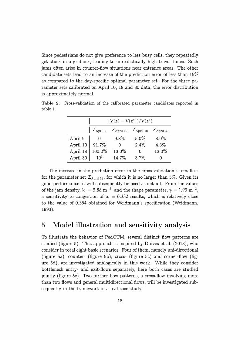
Table 1: Results of the calibration runs of four different days. For comparison,values reported by Weidmann (1993) are shown.

vf γ kc α β

April 9 1.20 1.50 4.42 2.44 0.005April 10 1.30 1.74 5.83 1.99 0.012April 18 1.22 1.95 5.88 2.08 2.55April 30 1.30 1.87 4.83 1.86 0.169

Weidmann 1.34 1.913 5.4 – –

It can be seen that the parameter values vary considerably across days.Nevertheless, all reported figures deviate less than 10% from the valuesreported by Weidmann (1993), except for April 9, where the deviation isslightly larger. The weight of the static floor field is estimated at between1.86 and 2.44 (between 1.86 and 2.08 without April 9). The calibrationdoes not yield an unambiguous estimate of the weight β, which is found inthe range between 0.005 and 2.55.

To evaluate the parameter candidates presented in table 1, each of themis applied to all four days. Table 2 shows the results of this cross-validation.A similar approach has been followed by Johansson et al. (2007), whoseefforts to calibrate the social force model have been mentioned in the in-troduction. They found that a broad range of parameter combinationsperforms almost equally well and applied a cross-validation on three datasets for choosing the optimal specification as well.

From table 2, it can be seen that the parameter set from the calibra-tion run corresponding to April 9 leads to very high errors. An analysishas revealed that the low value of β is at the root of the large deviation.

17

Since pedestrians do not give preference to less busy cells, they repeatedlyget stuck in a gridlock, leading to unrealistically high travel times. Suchjams often arise in counter-flow situations near entrance areas. The othercandidate sets lead to an increase of the prediction error of less than 15%as compared to the day-specific optimal parameter set. For the three pa-rameter sets calibrated on April 10, 18 and 30 data, the error distributionis approximately normal.

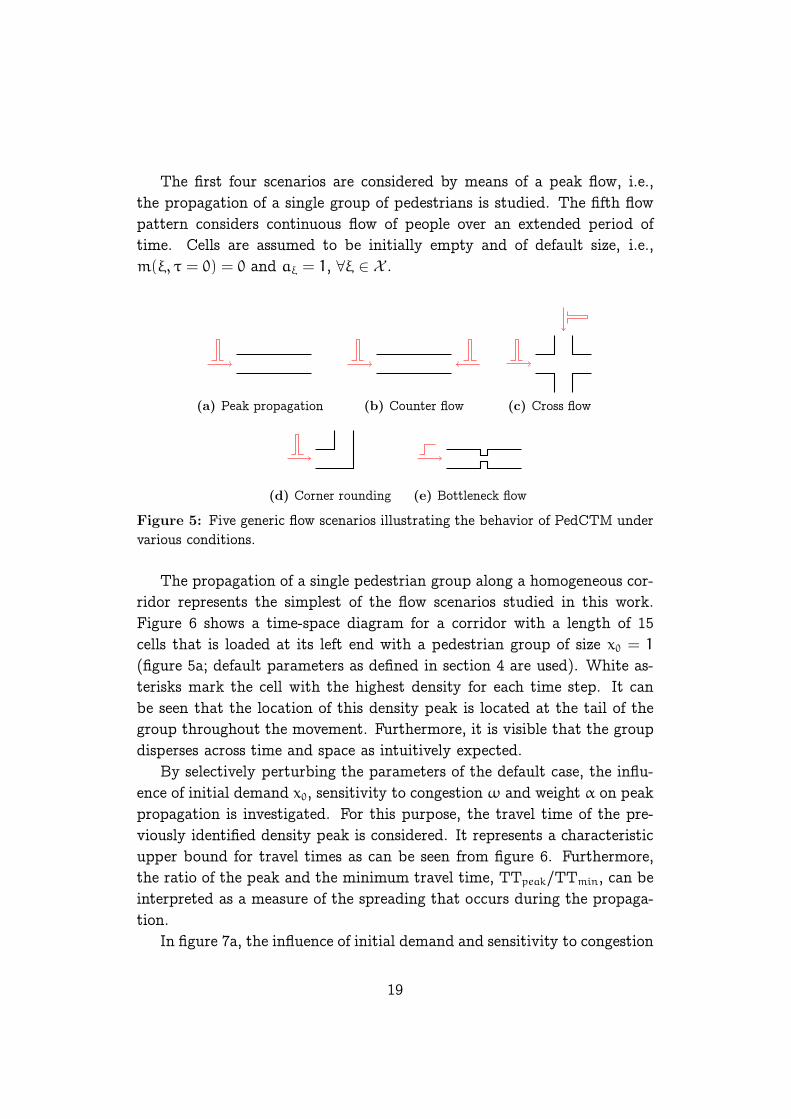
Table 2: Cross-validation of the calibrated parameter candidates reported intable 1.

(V(z) − V(z∗))/V(z∗)

ZApril 9 ZApril 10 ZApril 18 ZApril 30

April 9 0 9.8% 5.0% 8.0%April 10 91.7% 0 2.4% 4.3%April 18 100.2% 13.0% 0 13.0%April 30 103 14.7% 3.7% 0

The increase in the prediction error in the cross-validation is smallestfor the parameter set ZApril 18, for which it is no larger than 5%. Given itsgood performance, it will subsequently be used as default. From the valuesof the jam density, kc = 5.88 m−2, and the shape parameter, γ = 1.95 m−2,a sensitivity to congestion of ω = 0.332 results, which is relatively closeto the value of 0.354 obtained for Weidmann’s specification (Weidmann,1993).

5 Model illustration and sensitivity analysis

To illustrate the behavior of PedCTM, several distinct flow patterns arestudied (figure 5). This approach is inspired by Duives et al. (2013), whoconsider in total eight basic scenarios. Four of them, namely uni-directional(figure 5a), counter- (figure 5b), cross- (figure 5c) and corner-flow (fig-ure 5d), are investigated analogically in this work. While they considerbottleneck entry- and exit-flows separately, here both cases are studiedjointly (figure 5e). Two further flow patterns, a cross-flow involving morethan two flows and general multidirectional flows, will be investigated sub-sequently in the framework of a real case study.

18

The first four scenarios are considered by means of a peak flow, i.e.,the propagation of a single group of pedestrians is studied. The fifth flowpattern considers continuous flow of people over an extended period oftime. Cells are assumed to be initially empty and of default size, i.e.,m(ξ, τ = 0) = 0 and aξ = 1, ∀ξ ∈ X .

(a) Peak propagation (b) Counter flow (c) Cross flow

(d) Corner rounding (e) Bottleneck flow

Figure 5: Five generic flow scenarios illustrating the behavior of PedCTM undervarious conditions.

The propagation of a single pedestrian group along a homogeneous cor-ridor represents the simplest of the flow scenarios studied in this work.Figure 6 shows a time-space diagram for a corridor with a length of 15cells that is loaded at its left end with a pedestrian group of size x0 = 1

(figure 5a; default parameters as defined in section 4 are used). White as-terisks mark the cell with the highest density for each time step. It canbe seen that the location of this density peak is located at the tail of thegroup throughout the movement. Furthermore, it is visible that the groupdisperses across time and space as intuitively expected.

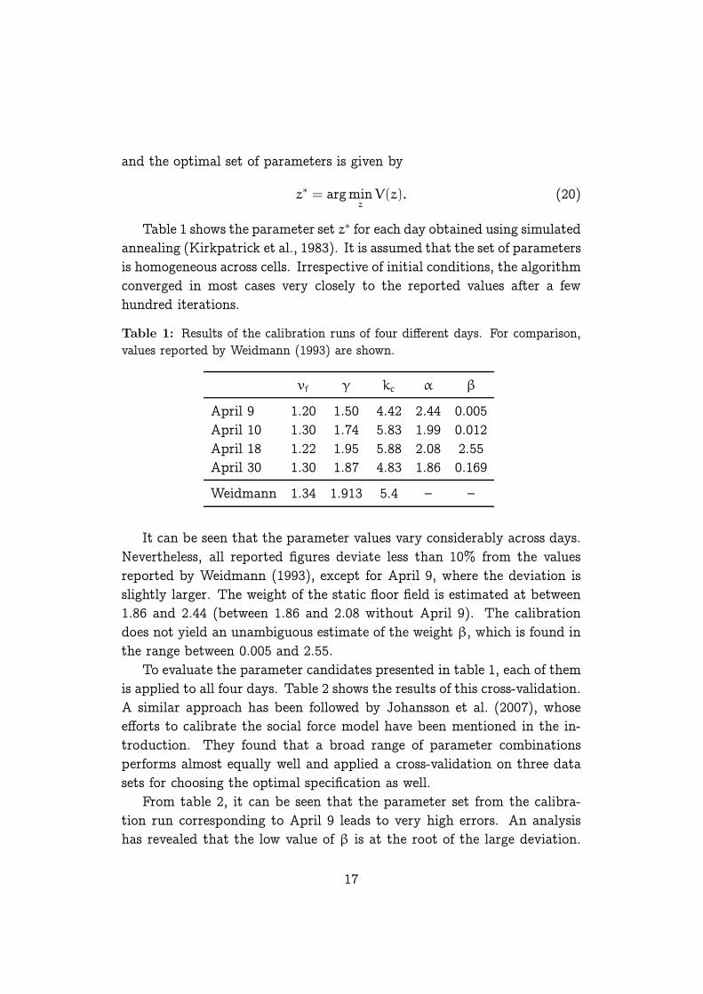
By selectively perturbing the parameters of the default case, the influ-ence of initial demand x0, sensitivity to congestion ω and weight α on peakpropagation is investigated. For this purpose, the travel time of the pre-viously identified density peak is considered. It represents a characteristicupper bound for travel times as can be seen from figure 6. Furthermore,the ratio of the peak and the minimum travel time, TTpeak/TTmin, can beinterpreted as a measure of the spreading that occurs during the propaga-tion.

In figure 7a, the influence of initial demand and sensitivity to congestion

19

1 5 10 151

5

10

15

20

26

ξ

τ

0

0.1

0.2

0.3

≥ 0.4

m(ξ, τ)

Figure 6: Time-space diagram of a pedestrian group propagating along a longi-tudinal corridor with a length of 15 cells. White asterisks mark for each time stepthe cell with the highest occupation, also referred to as the ‘concentration peak’(Parameters: x0 = 1, ω = 0.332, α = 2.08, β = 2.55).

on the peak travel time is shown. It can be seen that dispersion becomesmore important with increasing demand, following approximately a linearrelationship. The spreading is stronger for low values of ω, i.e., when thesensitivity to congestion is high. For low levels of demand, the peak traveltime is equal to the minimum travel time irrespective of the choice of ω.These observations are again in good agreement with intuitive expectations.

The weight of the static floor field has a similar impact on the ratioTTpeak/TTmin as can be seen from figure 7b. At low values of α, pedestri-ans do not systematically walk towards the destination. This is why evenfor a small demand, the peak travel time TTpeak can be several times largerthan TTmin. For small values of α, the spreading grows with increasing de-mand in a non-linear way, whereas for larger values of α, a linear increase inspreading is noticed. If α is set to zero, interestingly a moderate demandx0 ≈ 1 leads to the fastest propagation. Indeed, for α = 0, pedestriansare solely driven by the dynamic floor field to leave the high density areabuilt up around the inlet. For a very low demand, this effect is not signif-icant. For a high demand, the additional delay incurred by congestion isprominent and leads to an increased spreading. Therefore, an accelerated

20

0 2 4 6 80

2

4

6

8

ω ↑

x0

TT

peak/T

Tm

in

(a) α = 2.08, ω = {0.05, 0.1, 0.2, 0.332, 1, 10}

0 2 4 6 80

2

4

6

8

α ↑

x0

TT

peak/T

Tm

in

(b) α = {0, 0.1, 0.25, 0.5, 2.08}, ω = 0.332

Figure 7: Ratio of peak and minimum travel time as a function of the initialdemand for different values of (a) sensitivity to congestion ω and (b) weight α.The curve in red represents the default case with x0 = 1, α = 2.08, β = 2.55 andω = 0.322.

propagation results only for x0 ≈ 1. No results for α > 2.08 are shown,since the resulting curves almost coincide with the one obtained for defaultvalues.

Next, the interaction between two pedestrian groups propagating inopposite directions is investigated. This allows to study the superpositionof two approaching waves of pedestrians, and more specifically the build-up and dissolution of congestion occurring when they overlap and separate,respectively. Figure 8 shows the time-space diagram of a corridor consistingof 15 cells in length, which is loaded at both ends with a pedestrian groupof size x0 = 1. Default parameters are assumed.

It can be seen that up to time step τ = 7, the same pattern results asin figure 6. It follows a brief period of collision, during which both waveswiden significantly. The post-collision distribution is therefore much moredispersed. For lower values of ω, the spreading both before and duringthe collision would be even stronger, leading to longer travel times and aflatter distribution (results not shown).

A similar case of bi-directional flow arises when two pedestrian groupsmeet at an orthogonal crossing. Such a situation is more complex as itinvolves en-route path choice. Figure 9 shows four snapshots representingthe density pattern before, during, and after the collision in an orthogonal

21

1 5 10 151

5

10

15

20

25

30

ξ

τ

0

0.1

0.2

0.3

≥ 0.4

m(ξ, τ)

Figure 8: Time-space diagram of two colliding pedestrian waves in a homogeneouscorridor with a length of 15 cells (Parameters: x0 = 1, α = 2.08, β = 2.55,ω = 0.332).

cross-flow. Again an initial loading of x0 = 1 for each flow and defaultparameters are assumed.

The maximum cell density is reached at the top left of the central partof the crossing during the time period τ = 10 . . . 15 (figure 9b and c). Thistime range starts significantly after the first contact between the two groupsat τ = 4. The reason is that the peak concentration of a group is found atits tail, as it has been observed previously.

To quantitatively investigate the influence of the weights α and β onthe resulting flow pattern, the evolution of the cumulated arrivals η isinvestigated (figure 10). A semi-logarithmic scale allows to study theirinfluence over a large range of time.

From figure 10a it can be seen that the propagation is accelerated withan increasing weight of the static floor field. This observation is based ona computation with β = 2.55, but similar findings hold for other values ofβ. It means that people reach their destination earlier if they follow theshortest path more strictly. For a simple cross-flow scenario, such a resultis expected. It can however not be concluded that the same monotonicincrease is found for more complex geometries, in particular if the scenariois such that a gridlock is likely to occur when everyone follows the shortest

22

(a) τ = 5 (b) τ = 10

0

0.1

0.2

0.3

≥ 0.4

m(ξ, τ)

(c) τ = 15 (d) τ = 20

Figure 9: Density snapshots of a cross-flow scenario taken during four timeintervals before, during and after the collision between two orthogonally movingpedestrian groups (Parameters: α = 2.08, β = 2.55, ω = 0.332, x0 = 1).

path. Such a case has already been discussed in section 4.In contrast, the influence of the weight β on the evolution of cumulated

arrivals is not monotonic and generally smaller (figure 10b). For β ≤ 10,only a small deviation from the reference case is observed. For large valuesof β, the cumulated arrivals grow less rapidly due to the large influence ofcongestion on local path choice.

As suggested by Duives et al. (2013), corner-flow is studied as a furtherbasic flow pattern. Figure 11 shows three density snapshots of a corner-flow scenario obtained for default parameters and an initial demand x0 = 1.As expected, a region of high density is formed upstream the corner, andpedestrians walk around it following a curved path. This resembles wellthe empirically observed ‘corner rounding’ (Duives et al., 2013).

So far, the model behavior has been investigated by analyzing the prop-agation of distinct pedestrian groups. To further elucidate the influence of

23

1 1.5 2 2.5 30

0.2

0.4

0.6

0.8

1

α = 0

∞

log(τ)

η

(a) α = {0, 0.1, 0.25, 0.5, 1, 2.08, 100}, β = 2.55

1 1.5 2 2.5 30

0.2

0.4

0.6

0.8

1

log(τ)

η

β=0β=2.55β=10β=25β=100

(b) α = 2.08, β = {0, 2.55, 10, 25, 250}

Figure 10: Cumulated arrivals as a function of time for different values of α

(figure 10a) and β (figure 10b) for a cross-flow scenario (Parameters: x0 = 1 andω = 0.332).

the static and dynamic floor fields on local route choice, a continuous flowthrough a bottleneck in a longitudinal corridor is studied. The corridor ofinterest has a length of 22 and a width of 6 cells. At the bottleneck, thewidth is reduced to two cells. During the first 100 time steps, a continuousinflow of x = 1 is imposed.

For different parameter values, figure 12 shows the density distributionarising 100 time steps after the continuous inflow is stopped, i.e., at τ =

200. At this stage, pedestrians gradually propagate downstream, but the

(a) τ = 8 (b) τ = 16 (c) τ = 24

0

0.2

≥ 0.4

m(ξ, τ)

Figure 11: Density snapshots of a corner-flow scenario involving a single pedes-trian group propagating through a bent channel of three cells width (Parameters:α = 2.08, β = 2.55, ω = 0.332, x0 = 1).

24

dynamics of the model are relatively slow. The density pattern does notchange fundamentally in the time range τ ≈ 150 . . . 250 and is quasi non-transient.

(a) α = 2.08, β = 2.55 (η =

47.9%)(b) α = 1, β = 0 (η = 27.0%)

0

0.2

≥ 0.4

m(ξ, τ)

(c) α = 100, β = 0 (η = 51.7%) (d) α = 0, β = 0 (η = 0.21%)

Figure 12: Flow patterns arising in a corridor with bottleneck for a continuousloading. During the first 100 time steps, a continuous inflow of magnitude x = 1

is imposed. Snapshots show the computed density field for time interval τ = 200

for different values of α and β and a default sensitivity to congestion ω = 0.332.The cumulated fraction of people having arrived at the destination η(τ = 200) isindicated in brackets.

The weights α and β have a significant influence on en-route path choiceas can be seen from figure 12, in which a sensitivity to congestion of ω =

0.332 has been assumed. Four specific choices of α and β are considered:

Figure 12a (α = 2.08, β = 2.55, default case): Pedestrians take both thedistance to destination and local flow conditions into account for lo-cal path choice. Upstream of the bottleneck, all space is occupied.People act as if they were impatient to pass the bottleneck, which iswhy a broad zone of high density builds up in front of the bottleneck.This behavior is well known from pedestrian facilities in railway sta-tions (e.g. Daamen, 2004). This similarity is expected, as the usedparameter set has been calibrated for precisely this scenario. At timestep τ = 200, 47.9% of all pedestrians have arrived at the destination.Besides everyday flows with very high demand, this pattern seemsalso realistic for an emergency situation where people are impatientto pass a bottleneck.

Figure 12b (α = 1, β = 0): The density field shows that pedestrians walkalong paths that ‘anticipate’ the bottleneck. Most, but not all space

25

is occupied. Less than a third of the population has reached thedestination at τ = 200. If pedestrians have a good queueing discipline,or if traffic is low, such a flow pattern seems accurate.

Figure 12c (α = 100, β = 0): People strictly follow the shortest path, ir-respectively of flow conditions. Interestingly, this scenario yields thehighest fraction of people having reached the destination at τ = 200.This finding is to some extent analogous to the ‘faster-is-slower’ effectobserved for evacuation by Helbing et al. (2000), who found that alower desired velocity leads to a higher overall throughput. Here, itseems that a group of stoic pedestrians reaches its destination faster.This scenario represents an extreme case where pedestrians show aperfect queueing discipline or strictly minimize walking distance.

Figure 12d (α = 0, β = 0): When both weights are set to zero, the turn-ing proportions of each group are completely homogeneous. Thisleads to a high density at the inlet and a very slow propagation. Atτ = 200, only η = 0.22% of all pedestrians have reached the down-stream end. Such a situation might arise when people do not haveany idea where to go, and do not have any preference with respect tocongestion. If pedestrians give preference to less congested areas (e.g.α = 0, β = 1), the flow pattern still strongly resembles figure 12d,but propagation is marginally faster. Neither of the two situationsare very likely to be found in reality, but are reported for the sake ofcompleteness.

To conclude, we found that when a dense group of pedestrians movesacross space, its distribution gradually broadens over time. The peak con-centration is located at the tail. If two groups of pedestrians interact, ahigh density results in the area of collision, and the groups disperse signif-icantly. In an orthogonal layout with cross-flow, the highest densities arefound in cells where the two groups meet first, however significantly aftertheir first contact.

Three non-dimensional parameters have been identified that are key indescribing the model dynamics. The sensitivity to congestion ω controlsthe way in which the mean walking velocity is affected by pedestrian den-sity. A low value of ω implies that walking speed is significantly reducedwith increasing density. This reduction in speed leads to dispersion and

26

consequently to longer travel times. The weights α and β parametrizethe cell potential and thereby influence the en-route path choice. A largeweight of the static floor field yields generally shorter travel times sincepedestrians give a stronger preference to cells along the shortest path. Theweight of the dynamic floor field governs the attitude of pedestrians to-wards prevailing traffic conditions. For increasing values of β, pedestriansare more willing to take a detour if it allows avoiding congested areas. Thisoften leads to prolonged travel times, but can also be important in resolvinggridlock situations.

While PedCTM is able to reproduce a wide range of behavioral patternsfrom panic situations to disciplined queueing, it is originally designed todescribe everyday pedestrian flows in public spaces. Such a situation is dis-cussed in the following section that provides a detailed case study analysisof Lausanne railway station.

6 Case study and validation

To assess the practical applicability of PedCTM, a detailed analysis ofpedestrian flows in PU West of Lausanne railway station (see figure 4) iscarried out. The period between 07:40 and 07:45 in the morning peakhour of January 22, 2013, serves as case study. It represents the busiestfive-minute period throughout the day in Lausanne railway station. Whilefor calibration only the North part of PU West has been considered, forvalidation the complete pedestrian underpass is analyzed.

The performance of PedCTM is evaluated in two ways with respect topredictions of travel times and density levels. First, its results are com-pared with the ground truth that is available from tracking data. Second,PedCTM is compared with Viswalk (PTV, 2013, Version 5.40) that imple-ments the social force model (SFM; Helbing and Molnár, 1995). Introducedless than two decades ago, SFM is the current state of the art in pedestrianflow modeling.

For PedCTM, the default parameter set ZApril 18 is used, resulting in asimulation time step of length ∆t = ∆L/vf = 2.22 s. The same aggregationof space as described in section 4 is applied. For the simulation using SFM,default parameters of Viswalk are used, which are based on a calibrationperformed by Johansson et al. (2007). Pedestrian demand is aggregated in

27

60-second periods for Viswalk due to the lack of a suitable mechanism forusing a disaggregate origin-destination demand table as input. To accountfor stochasticity, five simulation runs are performed and the average iscalculated. More runs are not necessary, since only aggregated output isreported, which shows little fluctuation across the various runs. For bothPedCTM and SFM, the time period between 07:37 and 07:47 is computed,but only results for the period between 07:40 and 07:45 are reported inorder to remove a bias of an initially empty system.

In PU West, the most frequented route during the considered time pe-riod is the one connecting the main hall of the train station to the exteriorpart of platform 3/4. Table 3 shows the corresponding travel times for thetime period between 07:40 and 07:45. To allow for a comparison with thesocial force model, travel times are aggregated in periods of one minute.

Table 3: Travel times between the main hall of Lausanne railway station andthe exterior part of platform 5/6 (#5/6 West) according to tracking data (TTobs),the social force model (TTSFM), and PedCTM (TTPedCTM). The first two columnsshow overall demand (Xtot) and the demand along the route of interest (Xρ). Dataas observed on January 22, 2013.

Xtot Xρ TTobs TTSFM TTPedCTM

07:40 – 07:41 118 12 37.5± 4.8 36.7± 2.2 48.0± 4.0

07:41 – 07:42 343 20 45.0± 5.4 68.1± 27.3 53.2± 7.1

07:42 – 07:43 251 10 50.9± 2.8 63.0± 18.2 50.7± 5.1

07:43 – 07:44 199 8 39.8± 5.1 48.0± 15.3 48.6± 4.2

07:44 – 07:45 107 7 45.2± 3.1 40.1± 5.3 47.8± 3.9

During the time period of interest, the total demand in PU West fluc-tuates between 107 and 343 incoming pedestrians per minute (table 3).Despite being the most frequented route, the corresponding fraction ofpedestrians Xρ/Xtot is mostly below 10 %. Observed average travel timesvary between 37.5 and 50.9 s, i.e., over a range of 13.4 s.

According to PedCTM, the expected value of travel time varies be-tween 47.8 and 53.2 s, representing a relatively narrow range compared toobserved data. The social force model produces average travel times in therange between 36.7 and 68.1 s., which is larger than observed in the groundtruth. Overall, table 3 shows that PedCTM is able to correctly predict the

28

order of magnitude of travel times. However, due to the high stochasticitypresent in the observed data, it is difficult to draw conclusions about itspredictive power. A more aggregated validation of walking times seemsworthwhile.

Figure 13a shows a histogram of group-specific travel times accordingto pedestrian tracking data and as computed by PedCTM. The bin sizecorresponds to the simulation time step of PedCTM, i.e., the lowest avail-able level of aggregation. PedCTM slightly overestimates the frequency oftravel times beyond 70 s, and underestimates the occurrence of short traveltimes below 20 s.

0 20 40 60 80 100 1200

20

40

60

80

TT [s]

freq

uen

cy

observedPedCTM

(a) Observed vs. PedCTM (aggregation periodand diagram bin size equal to ∆t = 2.22 s)

0 20 40 60 80 100 1200

100

200

TT [s]

freq

uen

cyobservedPedCTMSFM

(b) Observed, SFM and PedCTM (aggregationover time period of 60 s, diagram bin size of 5 s)

Figure 13: Travel time distribution according to PedCTM, the social force model(SFM) and pedestrian tracking data.

To allow for a comparison with the social force model, figure 13b pro-vides a similar comparison of route-specific travel times with a temporalaggregation of 60 s. The resulting mean values are shown in a histogramwith a bin size of 5 s. As seen previously, PedCTM overestimates the occur-rence of long travel times, but otherwise shows a reasonable agreement withtrajectory data. The social force model seems to overestimate small traveltimes and to underestimate the most frequently observed travel times inthe range between 35 and 55 s. Overall, the agreement between PedCTMand trajectory data is better than for SFM if the squared error is considered(114.4 vs. 181.6).

A comparison of the predicted and measured travel time distribution

29

for an individual route yields a similar result as for the overall distribution.Figure 14 shows the result for the busiest route, main hall to #5/6 West,that has already been investigated in table 3.

0 20 40 60 80 100 1200

5

10

15

TT [s]

freq

uen

cy

observedPedCTM

Figure 14: Travel time distribution corresponding to the busiest route in PUWest in the time period between 7:40 – 7:45 on January 22, 2013 according toPedCTM and pedestrian tracking data.

PedCTM is unable to describe the ‘faster’ half of the travel time dis-tribution, i.e., walking times that are shorter than the theoretical free-flowtravel time. For instance, the shortest observed travel time for the routeand time interval of interest amounts to 30.9 s, which corresponds to anaverage walking speed of 1.75 m/s. An analysis of other routes shows gen-erally similar results, even though the mismatch between prediction andobservation is mostly smaller.

Figure 15 shows the residuals of group-specific travel times computedusing PedCTM compared to tracking data. The distribution of the absoluteand the relative error is provided in figure 15a and 15b, respectively. Ina first approximation, the histograms resemble a normal distribution withzero mean. From figure 15a, it can be seen that the predicted travel timesdeviate less than 10 s from the observed walking times for two thirds of thepedestrian groups. For less than 10% of all groups, the deviation is largerthan 20 s. In relative terms, 50% of the estimates deviate less than 13%from observed values, and for more than 80% of all groups the relative error

30

is smaller than 33%. Also, it can be seen from the absolute residuals thatthere are a few particularly long walking times which cannot be reproducedby PedCTM at all.

−100 −50 0 500

50

100

150

TTℓ,PedCTM − TTℓ,observed [s]

freq

uen

cy

(a) Absolute error

−1 −0.5 0 0.5 10

20

40

60

80

100

TTℓ,PedCTM/TTℓ,observed − 1

freq

uen

cy

(b) Relative error

Figure 15: Absolute and relative residuals of travel time predictions by PedCTMfor each pedestrian group ℓ, weighted by group size Xρℓ,τℓ . Group-specific traveltimes are not readily available for the social force model from the used implemen-tation and therefore not shown.

In conclusion, it can be noted that PedCTM is able to generate traveltime predictions that are in reasonable agreement with observations. How-ever, it underestimates very long travel times (see left tail of distribution infigure 15a). A reason for this discrepancy might be non-walking behaviorof pedestrians, such as purchasing a ticket or checking the train timetable.These activities are not considered by the pedestrian walking model. Sim-ilarly, PedCTM fails at predicting very short travel times corresponding toaverage velocities that are higher than the free-flow speed. Both shortcom-ings are due to the assumption of a deterministic fundamental diagram,which associates with each density exactly one speed. In particular, itdoes not take into account that some pedestrians show walking speeds thatare significantly higher than what is commonly acknowledged as free-flowspeed in the literature. We believe that these limitations could be overcomeby incorporating a stochastic fundamental diagram (Nikolic et al., 2013),which is subject to further research.

Besides walking times, density is an important indicator of level of ser-vice in pedestrian facilities. Figure 16 shows the density maps of PU West

31

as calculated from pedestrian tracking data, and as computed by the socialforce model and PedCTM. A discrete LOS scale ranging from A (‘good’) toF (‘bad’) is used for comparison (Highway Capacity Manual, 2000, Exhibit18-3).

In the captions of figure 16, train arrivals relevant for each time intervalare indicated. Train arrivals induce dense pedestrian waves that propa-gate through walking facilities and potentially lead to congestion. Boththe social force model and PedCTM are able to reproduce the evolution oflocal pedestrian density relatively well. The highest pedestrian densitiesare observed between 7:41 and 7:43 due to various incoming trains. Thelevel of service is in the range between A and E, i.e., densities are gen-erally below 1.333 m−2. Both PedCTM and SFM seem to underestimatethe level of congestion during the peak minutes 07:41–07:44. Accordingto the observed data, a region of high density forms along the center lineof the corridor. In the two models, space is occupied more evenly, i.e.,densities are overestimated laterally, and underestimated along the centerline. During the time interval 07:42–07:43, SFM produces a gridlock situa-tion in the narrow part of PU West. Specifically, pedestrians coming fromNorth collide with pedestrians entering PU West from platform #5/6. Asa consequence, locally a very high density exceeding 1.333 m−2 results (fig-ure 16c) and travel times are significantly overestimated (table 3). Thissituation was observed in all five runs. In the ground truth, such a gridlockis not present. A detailed analysis shows that SFM is prone to predictinggridlocks also in other situations involving PU West (Hänseler et al., 2012).In contrast, PedCTM does not suffer from this shortcoming and thus seemsbetter suited for infrastructure assessment in this particular case. In fig-ure 16, PedCTM correctly predicts the local service level for 58.2% of alldiscretization cells, whereas for SFM an accuracy of 54.6% results.

Overall, despite the mentioned shortcomings, PedCTM is able to com-pute travel time distributions and density maps that are in agreement withobserved data. In the case study considered above, it performed slightlybetter than SFM. Presumably, the performance of SFM can be improved bya dedicated calibration, but as it has been argued, this is a difficult task fordisaggregate models. Thanks to its aggregate nature and the deterministiccharacter, the computational cost of PedCTM is relatively low. A Java im-plementation of PedCTM without multi-threading is able to compute theabove case study of PU West about ten times faster than Viswalk, a highly

32

obs

SFM

PedCTM

(a) 7:40–7:41: Relatively low occupation.

obs

SFM

PedCTM

(b) 7:41–7:42: Arrival of train IR 1606 at7:40:20 on platform 3/4.

obs

SFM

PedCTM

(c) 7:42–7:43: Arrival of train IR 706 at7:41:24 on platform 5/6.

obs

SFM

PedCTM

(d) 7:43–7:44: Arrival of train IR 1407 at7:42:20 on platform 3/4.

obs

SFM

PedCTM

(e) 7:44–7:45: Gradual decrease in pedes-trian occupation.

LOS Pedestrian density

A k < 0.179 [m−2]B 0.179 ≤ k < 0.270C 0.270 ≤ k < 0.455D 0.455 ≤ k < 0.714E 0.714 ≤ k < 1.333F 1.333 ≤ k

Figure 16: Pedestrian density map of PU West in Lausanne railway station forthe time period between 7:40 and 7:45 on January 22, 2013. For each time periodof one minute, the resulting maps obtained from pedestrian tracking data (obs),the social force model (SFM), and from PedCTM are shown. The color scale is asprovided by NCHRP for pedestrian walkways (Highway Capacity Manual, 2000,Exhibit 18-3).

33

optimized implementation of the social force model.

7 Concluding remarks

In this work, we presented a novel framework for modeling pedestrians flowsin transportation hubs and other public spaces. Such flows are typicallymulti-directional, non-stationary, and often congested during peak hours.

The proposed model considers space as a two-dimensional network ofhomogeneous cells. Each cell is part of a particular area, such as ‘stationhall’ or ‘train platform #1’. Most areas contain more than one cell, andsequences of connected areas form routes. Pedestrians are organized ingroups, which are characterized by a route, a departure time interval, anda size.

To account for en-route path choice, a discrete choice model in combina-tion with the concept of cell potentials is introduced. The cell potential con-sists of a static, route-specific component, and a dynamic, traffic-dependentpart. Pedestrians are assumed to move in the direction of decreasing po-tential, i.e., they gradually propagate along their route, avoiding congestedcells to the extent possible.

A modified cell-transmission model (CTM) is used to calculate flowsbetween cells. For each pair of adjacent cells, group-specific sending ca-pacities for the emitting cell, and a receiving capacity for the destinationcell are computed. In absence of congestion, all sending capacities are ac-commodated. Otherwise, the receiving capacity is distributed following ademand-proportional supply scheme. This concept allows for studying thejoint propagation of multiple pedestrian groups following different routes,assigning pedestrian flows in space, and better understanding phenomenasuch as congestion and dissolution of jams.

Our approach differs from related pedestrian propagation models in sev-eral aspects. First, its foundation on CTM allows for a realistic descriptionof movement patterns under most flow conditions and at a relatively lowcost. Compared to other CTM-based models, we use a dedicated fundamen-tal diagram for pedestrian flows. Second, it provides a consistent modelingframework for multi-directional flows and local path choice. The model ar-chitecture allows to individually track the propagation of pedestrian groupsacross space and time. Third, the whole model is rigorously calibrated on

34

real pedestrian tracking data. The obtained model parameters are in goodagreement with the literature.

Several properties of the presented model are explored by consideringfive generic test cases. First, the propagation of a pedestrian group along acorridor is investigated. Dispersion over time and space for different choicesof parameters is discussed. It is shown that the peak concentration of apropagating pedestrian group is typically found at its tail. Furthermore, acounter and cross-flow scenario, corner rounding as well as a bottleneck floware investigated. The influence of the cell potential on local path choice,and its impact on travel times are investigated in detail. Depending on theparametrization of the cell potential, the resulting flows resemble differentbehavioral patterns ranging from evacuation to patient queueing.

Subsequently, the model is applied to a real case study involving apedestrian underpass in Lausanne railway station, Switzerland. A partic-ularly busy five-minute period with over a thousand arriving pedestriansis considered. The model developed in this work is able to reproduce theoverall travel time distribution and to generate realistic pedestrian den-sity maps. However, it fails in predicting travel times corresponding towalking speeds that are faster than free-flow velocities as well as very slowtravel times caused by non-walking behavior. Despite these shortcomings,a comparison with trajectory data and the social force model (Helbing andMolnár, 1995, SFM) shows a good performance of the developed model.Moreover, its computational cost is about one order of magnitude lower ascompared to SFM.

To conclude, the proposed model provides an aggregate approach forstudying large-scale problems of crowd dynamics in congested pedestrianfacilities. It shows a realistic behavior due to its foundation on an empiri-cal fundamental diagram and the performed systematic calibration. Due toits low computational requirements compared to disaggregate models suchas the above mentioned social force model, it can be readily integrated ina real-time pedestrian flow simulator, considering dynamic demand esti-mation and assignment. Efforts along these lines are currently ongoing inour group. Furthermore, the use of a stochastic fundamental diagram isenvisaged, as it likely will allow to explicitly model random fluctuations inwalking time observed e.g. in the pedestrian tracking data presented in thiswork. In particular, this approach will allow considering different speedsfor different classes of pedestrians such as ‘business travelers’, ‘commuters’,

35

‘seniors’, and so on.

Acknowledgement

Financial support by SNF grant #200021-141099 ‘Pedestrian dynamics:flows and behavior’ as well as by SBB-CFF-FFS in the framework of ‘Ped-Flux’ is gratefully acknowledged.

References

Abdelghany, A., Abdelghany, K., Mahmassani, H. S., Al-Zahrani, A.,2012. Dynamic simulation assignment model for pedestrian movementsin crowded networks. Transportation Research Record: Journal of theTransportation Research Board 2316 (1), 95–105.

Al-Gadhi, S. A., Mahmassani, H. S., 1991. Simulation of crowd behaviorand movement: fundamental relations and application. TransportationResearch Record 1320 (1320), 260–268.

Alahi, A., Jacques, L., Boursier, Y., Vandergheynst, P., 2011. Sparsitydriven people localization with a heterogeneous network of cameras. Jour-nal of Mathematical Imaging and Vision 41 (1-2), 39–58.

Antonini, G., 2005. A discrete choice modeling framework for pedestrianwalking behavior with application to human tracking in video sequences.Faculty of Science and Technology in Engineering.

Asano, M., Sumalee, A., Kuwahara, M., Tanaka, S., 2007. Dynamic celltransmission-based pedestrian model with multidirectional flows andstrategic route choices. Transportation Research Record: Journal of theTransportation Research Board 2039 (1), 42–49.

Ashok, K., Ben-Akiva, M. E., 2000. Alternative approaches for real-timeestimation and prediction of time-dependent origin–destination flows.Transportation Science 34 (1), 21–36.

Ben-Akiva, M. E., Bierlaire, M., Burton, D., Koutsopoulos, H. N., Misha-lani, R., 2001. Network state estimation and prediction for real-time traf-fic management. Networks and Spatial Economics 1 (3-4), 293–318.

36

Ben-Akiva, M. E., Lerman, S. R., 1985. Discrete choice analysis: theoryand application to predict travel demand. Vol. 9. MIT Press.

Bierlaire, M., Crittin, F., 2006. Solving noisy, large-scale fixed-point prob-lems and systems of nonlinear equations. Transportation Science 40 (1),44–63.

Blue, V., Adler, J., 2001. Cellular automata microsimulation for model-ing bi-directional pedestrian walkways. Transportation Research Part B:Methodological 35 (3), 293–312.

Cascetta, E., Inaudi, D., Marquis, G., 1993. Dynamic estimators of origin-destination matrices using traffic counts. Transportation Science 27 (4),363–373.

Cascetta, E., Postorino, M. N., 2001. Fixed point approaches to the es-timation of O/D matrices using traffic counts on congested networks.Transportation Science 35 (2), 134–147.

Çetın, N., 2005. Large-scale parallel graph-based simulations. Ph.D. thesis,ETH Zürich.

Charypar, D., 2008. Efficient algorithms for the microsimulation of travelbehavior in very large scenarios. Ph.D. thesis, ETH Zürich.

Cheah, J. Y., Smith, J. M., 1994. Generalized M/G/c/c state dependentqueueing models and pedestrian traffic flows. Queueing Systems 15 (1),365–386.

Daamen, W., 2004. Modelling passenger flows in public transport facilities.Ph.D. thesis, Delft University of Technology.

Daganzo, C., 1994. The cell transmission model: A dynamic representationof highway traffic consistent with the hydrodynamic theory. Transporta-tion Research Part B: Methodological 28 (4), 269–287.

Daganzo, C., 1995. The cell transmission model, Part II: Network traffic.Transportation Research Part B: Methodological 29 (2), 79–93.

Dijkstra, E. W., 1959. A note on two problems in connexion with graphs.Numerische mathematik 1 (1), 269–271.

37

Duives, D. C., Daamen, W., Hoogendoorn, S. P., 2013. State-of-the-art crowd motion simulation models. Transportation Research Part C:Emerging Technologies 37 (12), 193–209.

Guo, R., Huang, H., Wong, S., 2011. Collection, spillback, and dissipa-tion in pedestrian evacuation: A network-based method. TransportationResearch Part B: Methodological 45 (3), 490–506.

Hänseler, F., Molyneaux, N., Thémans, M., Bierlaire, M., 2013. Pedestrianstrategies within railway stations: Analysis and modeling of pedestrianflows (PedFlux Mid-Term Report). Tech. rep., EPFL.

Hänseler, F., Sahaleh, S., Farooq, B., Lavadinho, S., Thémans, M., Bier-laire, M., 2012. Final report on the modeling part of the ‘Flux piétonsGare de Lausanne’ project within the framework of ‘Léman 2030’. Tech.rep., EPFL.

Helbing, D., Farkas, I., Vicsek, T., 2000. Simulating dynamical features ofescape panic. Nature 407 (487–490).

Helbing, D., Molnár, P., 1995. Social force model for pedestrian dynamics.Physical review E 51 (5), 4282–4286.

Highway Capacity Manual, 2000. Transportation Research Board. Wash-ington, DC.

Hoogendoorn, S., Bovy, P., 2004. Pedestrian route-choice and activityscheduling theory and models. Transportation Research Part B: Method-ological 38 (2), 169–190.

Hoogendoorn, S. P., Bovy, P. H., 2001. State-of-the-art of vehicular trafficflow modelling. Proceedings of the Institution of Mechanical Engineers,Part I: Journal of Systems and Control Engineering 215 (4), 283–303.

Hoogendoorn, S. P., Daamen, W., 2007. Microscopic calibration and vali-dation of pedestrian models: Cross-comparison of models using experi-mental data. In: Traffic and Granular Flow’05. Springer, pp. 329–340.

Hughes, R. L., 2002. A continuum theory for the flow of pedestrians. Trans-portation Research Part B: Methodological 36 (6), 507–535.

38

Johansson, A., Helbing, D., Shukla, P. K., 2007. Specification of the so-cial force pedestrian model by evolutionary adjustment to video trackingdata. Advances in Complex Systems 10 (2), 271–288.

Kesting, A., 2012. Traffic Flow Dynamics: Data, Models and Simulation.Springer.

Kirkpatrick, S., Jr., D. G., Vecchi, M. P., 1983. Optimization by simmulatedannealing. Science 220 (4598), 671–680.

Løvås, G. G., 1994. Modeling and simulation of pedestrian traffic flow.Transportation Research Part B: Methodological 28 (6), 429–443.

Mahmassani, H. S., 2001. Dynamic network traffic assignment and simu-lation methodology for advanced system management applications. Net-works and Spatial Economics 1 (3-4), 267–292.

Nikolic, M., Bierlaire, M., Farooq, B., 2013. Spatial tessellations of pedes-trian dynamics, 2nd Symposium of the European Association for Re-search in Transportation, September 05, 2013, Stockholm, Sweden.

Osorio, C., Bierlaire, M., 2009. An analytic finite capacity queueing networkmodel capturing the propagation of congestion and blocking. EuropeanJournal of Operational Research 196 (3), 996–1007.

PTV, 2013. VISSIM 5.40 User Manual.URL http://vision-traffic.ptvgroup.com

Rahman, K., Ghani, N. A., Kamil, A. A., Mustafa, A., Chowdhury, M.A. K., 2013. Modelling pedestrian travel time and the design of facilities:A queuing approach. PloS ONE 8 (5), e63503.

Robin, T., Antonini, G., Bierlaire, M., Cruz, J., 2009. Specification, esti-mation and validation of a pedestrian walking behavior model. Trans-portation Research Part B: Methodological 43 (1), 36–56.

Seyfried, A., Steffen, B., Klingsch, W., Boltes, M., 2005. The fundamentaldiagram of pedestrian movement revisited. Journal of Statistical Mechan-ics: Theory and Experiment 2005 (10), P10002.

39

Sherali, H. D., Park, T., 2001. Estimation of dynamic origin–destinationtrip tables for a general network. Transportation Research Part B:Methodological 35 (3), 217–235.

Weidmann, U., 1993. Transporttechnik der Fussgänger. Institute for Trans-port Planning and Systems, ETH Zürich.

40