Embed Size (px)
Citation preview

East Tennessee State UniversityDigital Commons @ East
Tennessee State University
Electronic Theses and Dissertations Student Works
8-2014
An Agent-Based Model of Ant Colony Energy andPopulation Dynamics: Effects of Temperature andFood FluctuationGuo XiaohuiEast Tennessee State University
Follow this and additional works at: https://dc.etsu.edu/etd
Part of the Behavior and Ethology Commons, Biology Commons, and the Population BiologyCommons
This Thesis - Open Access is brought to you for free and open access by the Student Works at Digital Commons @ East Tennessee State University. Ithas been accepted for inclusion in Electronic Theses and Dissertations by an authorized administrator of Digital Commons @ East Tennessee StateUniversity. For more information, please contact [email protected].
Recommended CitationXiaohui, Guo, "An Agent-Based Model of Ant Colony Energy and Population Dynamics: Effects of Temperature and FoodFluctuation" (2014). Electronic Theses and Dissertations. Paper 2395. https://dc.etsu.edu/etd/2395
An Agent-Based Model of Ant Colony Energy and Population Dynamics:
Effects of Temperature and Food Fluctuation
____________________
A thesis
presented to
the faculty of the Department of Biological Sciences
East Tennessee State University
In partial fulfillment
of the requirements for the degree
Masters of Science in Biology
______________________
by
Xiaohui Guo
August 2014
_______________________
Dr. Istvan Karsai, Chair
Dr. Thomas F. Laughlin
Dr. Christopher D. Wallace,
Keywords: Ant colony, agent-based model, metabolic theory of ecology, energy dynamic, Kruskal-Wallis test

2
ABSTRACT
An Agent-Based Model of Ant Colony Energy and Population Dynamics:
Effects of Temperature and Food Fluctuation
by
Xiaohui Guo
The ant colony, known as a self-organized system, can adapt to the environment by a series of
negative and positive feedbacks. There is still a lack of mechanistic understanding of how the
factors, such as temperature and food, coordinate the labor of ants. According to the Metabolic
Theory of Ecology (MTE), the metabolic rate could control ecological process at all levels. To
analyze self-organized process of ant colony, we constructed an agent-based model to simulate
the energy and population dynamics of ant colony. After parameterizing the model, we ran 20
parallel simulations for each experiment and parameter sweeps to find patterns and dependencies
in the food and energy flow of the colony. Ultimately this model predicted that ant colonies can
respond to changes of temperature and food availability and perform differently. We hope this
study can improve our understanding on the self-organized process of ant colony.

3
DEDICATION
I dedicate this thesis to my parents Xing Guo and Hexian Fan who have constantly shown
keen interest and invested in my education. I also dedicate this work to my girlfriend, Wenjing
Mu, who supported and encouraged me to make this work successful.
4
ACKNOWLEDGEMENTS
I want to express my sincere gratitude to Dr. Istvan Karsai, Associate Professor,
Department of Biological Sciences, East Tennessee State University (ETSU) for his acceptance
to work with me. I really appreciate the training and research techniques I learned from him that
helped to improve the understanding of every aspect of my research. It is my honor to work with
him to study ant colony models.
I also thank Dr. Thomas F. Laughlin, Department of Biological Sciences, ETSU for being
part of my thesis committee. I really appreciate the useful suggestions he gave me. I also thank
Dr. Christopher D. Wallace, Department of Computer Sciences, ETSU for his immersed
contribution as a member of my thesis committee towards this work.
I am also grateful for the School of Graduate Studies of ETSU for awarding me the
Thesis Scholarship to support our research.

5
TABLE OF CONTENTS
Page
ABSTRACT .....................................................................................................................................2
DEDICATION .................................................................................................................................3
ACKNOWLEDGEMENTS .............................................................................................................4
LIST OF TABLES ...........................................................................................................................9
LIST OF FIGURES .......................................................................................................................10
Chapter
1.INTRODUCTION ......................................................................................................................12
Ant’s Sensitivity to the Ecological Event .........................................................................12
Climate Change Effects on Animals .................................................................................13
Allometric Equation for Metabolism ...............................................................................15
The Significance of Ant Workers in Population and Energy Dynamics of Ant Colony ...17
2. MATERIALS AND METHODS ...............................................................................................19
Purpose .............................................................................................................................19
State Variables and Scales ................................................................................................19
Process Overview and Scheduling ...................................................................................22
Design Concepts ...............................................................................................................26
Emergence ..............................................................................................................26
Adaptation and Fitness ...........................................................................................27

6
Chapter Page
Sensing ...................................................................................................................27
Interactions .............................................................................................................27
Stochasticity ...........................................................................................................28
Collectives..............................................................................................................28
Observation ............................................................................................................29
Initialization ......................................................................................................................29
Parameters ........................................................................................................................30
Input ..................................................................................................................................32
Submodels ........................................................................................................................33
The Tasks of Agents ...............................................................................................33
Interactions .............................................................................................................35
Changing of Tasks ..................................................................................................36
Energy and Mass ....................................................................................................37
Monitored Values ...................................................................................................39
Experiment .......................................................................................................................40
Experiment of Temperature Changes .....................................................................40
Experiment of Food Availability Changes .............................................................41
Experiment of Climate Changes ............................................................................41
3. RESULTS ...................................................................................................................................42

7
Chapter Page
Effects of Seasonal Temperature Change on Population and Energy Dynamic of Ant
Colony ..............................................................................................................................42
Effects of Temperature Elevations on Population and Energy Dynamic of the Ant
Colony ..............................................................................................................................45
Effects of Food Availabilities on Population and Energy Dynamic of Ant Colony .........51
Effects of High Food Richness and Temperature on Population and Energy Dynamic
of Ant Colony ...................................................................................................................54
4. DISCUSSION ............................................................................................................................58
Seasonal Dynamics of Ant Colonies ................................................................................58
Effects of Temperature on Population and Energy Dynamic of Ant Colony ...................59
Effects of Food Richness on Population and Energy Dynamic of Ant Colony ................63
Effects of Both Food and Temperature on Population and Energy Dynamic of Ant
Colony ..............................................................................................................................64
5. CONCLUSIONS........................................................................................................................67
REFERENCES ..............................................................................................................................68
APPENDICES ...............................................................................................................................79
APENDIX A: Standard Metabolic Rate ...........................................................................79
APENDIX B: Metabolic Rate for Locomotion ................................................................80
APENDIX C: Metabolic Rate for Growth, Reproduction, and Biosynthesis ..................81

8
APENDIX D: Amount of the Food per One Bite .............................................................83
APENDIX E: Relationship among Photosynthesis, Temperature, and CO2 ....................84
VITA ..............................................................................................................................................85
9
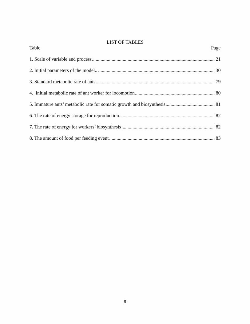
LIST OF TABLES Table Page
1. Scale of variable and process .................................................................................................... 21
2. Initial parameters of the model.. ............................................................................................... 30
3. Standard metabolic rate of ants ................................................................................................. 79
4. Initial metabolic rate of ant worker for locomotion ................................................................. 80
5. Immature ants’ metabolic rate for somatic growth and biosynthesis ........................................ 81
6. The rate of energy storage for reproduction .............................................................................. 82
7. The rate of energy for workers’ biosynthesis ............................................................................ 82
8. The amount of food per feeding event ...................................................................................... 83

10
LIST OF FIGURES Figure Page 1. Process of overview of the model.. ........................................................................................... 26
2. Partitioning of energy assimilated from food. .......................................................................... 37
3. Population dynamics in single simulations. .............................................................................. 44
4. Average value of 20 parallel simulations with constant temperature and dynamic
temperature. ....................................................................................................................45
5. Effects of temperature elevation regime on (a) energy of colonies, (b) population size of
colonies, (c) energy of colonies on the 270th day, and (d) average population of
colonies on the 270th day.. ...............................................................................................46
6. Two cases of colony extinction at the 14oC elevated temperature regime. ............................... 47
7. Effects of temperature elevated regime on birth rate of immature ants.. .................................. 47
8. Effects of temperature elevated regime on developmental time of immature ants. .................. 48
9. Effects of temperature elevated regimes on hunger rate of workers......................................... 49
10. Effects of temperature elevated regime on foraging efficiency. ............................................. 50
11. Effects of temperature elevation regime on (a) average mass of workers, (b) the average
mass of workers on the 200 th day.. ............................................................................... 51
12. Effects of temperature elevated regime on nursing efficiency.. .............................................. 51
13. Effects of food availability on (a) energy of colonies, (b) population size of colonies, (c)
energy of colonies on the 270th day, and (d) population of colonies on the 270th day. 52
14. Effects of food availability on food storage. ........................................................................... 53
15. Effects of food availability on (a) foraging efficiency and (b) nursing efficiency.. ................ 53
16. Effects of food availability on birth rate of immature ants.. ................................................... 54

11
Figure Page
17. Effects of high temperature and food richness on (a) energy of colonies, (b) population
size of colonies, (c) energy of colonies on the 270th day, and (d) population of
colonies on the 270th day.. .............................................................................................. 56
18. Effects of high temperature and food richness on birth rate of immature ants.. ..................... 56
19. Effects of high temperature and food richness on hunger rate of workers.. ........................... 57
20. Effects of high temperature and food richness on foraging efficiency.. ................................. 57
21. Effects of high temperature and food richness on nursing efficiency.. ................................... 57
22. Relationship between photosynthetic rate and temperature. ................................................... 65
23. Feedbacks’ networks of ant colony. ........................................................................................ 66

12
CHAPTER 1
INTRODUCTION
Ant’s Sensitivity to the Ecological Event
Insects make good indicators of ecological condition because they are highly diverse and
functionally important, can integrate ecological processes, and are sensitive to environmental
change (Brown 1997). As one of the famous terrestrial insect, ants have the critical ecological
roles in soil turnover and structure (Humphreys 1981; Lobry de Bruyn and Conacher 1994),
nutrient cycling (Levieux 1983; Lal 1988), plant protection, seed dispersal, and seed predation
(Ashton 1979; Beattie 1985; Christian 2001). Ants have proven sensitive and rapid responders to
environmental variables (Campbell and Tanton 1981; Majer 1983; Andersen 1990). In recent
analysis of various insect groups as potential bioindicators, ants scored highest (Brown 1997).
They have been used as bioindicators to manage mining site restoration because both their
abundance and species richness will decline with increasing dry sulfur deposition from mining
emissions (Hoffmann 2003). Forest management agencies in Australia also have incorporated
ants in monitoring programs associated with fire and logging practices (Andersen 1997). The
rapid replacement of the ecologically complex regrowth forest through wildfire and salvage
logging caused a substantial increase in ant’s foraging activity (P. pallidus) during the first
postfire autumn period, and activity remained high for up to 14 months (Neuman 1992). In the
coffee agroecosystem in Central America, it was found that microclimate changes, high-light
environment, and lack of leaf litter cover in the unshaded system are the determinants of the
differences in ground foraging ant diversity (Perfecto and Vandermeer 1996). Monitoring a
single species of ant is also recommended to detect trends among threatened and endangered or
keystone species (Underwood and Fisher 2006). Ants are important seed dispersers. Their

13
abundance and diversity can also be used to monitor the ecosystem function performed (Majer
1984; Grimbacher and Hughes 2002). Relying on the ant-seed interactions to bush regeneration,
the varied proportion of ant species indicates the differences of zone types significantly
(Grimbacher and Hughes 2002). In the environment destroyed by grazing and trampling, ant
species diversity can respond to these disturbances. For example, in the remnant Eucalyptus
salubris woodland disturbed by sheep grazing, lower ant diversity was recorded (Abensperg-
Traun 1996), and in grasslands at Mount Piper, Victoria, Australia, the same relationship
between grazing and ant species richness was detected as well (Miller 1997). The ant community
could respond to the habitat fragmentation by declining population sizes as well. Comparing
twig-dwelling ants between two 100 ha forest fragments with 2 continuous areas of forest in the
Amazon, Carvalho and Vasconcelos (1999) found species richness and abundance to be higher in
continuous forest sites than isolated fragment sites. Recently, researchers focused on the
responses of ant communities to climate change. By analyzing several niches models, Argentine
ants (Linepithema humile Mayr) was predicted to retract its range in tropical regions but to
expand at higher latitude areas (Roura-Pascual et al. 2004). Retrospecting the adaptation history
of ants on climate, Dunn et al. (2009) suggested that the hemispherical asymmetry of ant species
distribution was caused by greater climate change since the Eocene in the northern than in the
southern hemisphere that made more extinctions in the northern hemisphere with consequent
effects on local ant species richness. Meanwhile, Kaspari (2005) also found the number and
mass of workers influenced by NPP (net primary productivity, g of carbon per m2 per year), and
temperature will determine the ant colony mass independently under climate change.
Climate Change Effects on Animals
Climate change is a significant and lasting change in the statistical distribution

14
of weather patterns over periods ranging from decades to millions of years. It is caused by
factors such as biotic processes, variations in solar radiation received by Earth, plate tectonics,
and volcanic eruptions. Certain human activities have also been identified as significant causes
of recent climate change, often referred to as "global warming" (National Research
Council 2010). Climate change does not only cause changes in the climate system ranging from
annual precipitation and solar radiation to global land-ocean temperature increment but also
affects the biodiversity in land-based ecosystem and ocean ecosystem. In recent major ice ages,
the climate change caused distribution changes of most living organisms. As an example of
Chorthippus parallelus, the common meadow grasshopper of Europe across all northern Europe,
their haplotypes showed little diversity and were similar to those in the Balkans, clearly
indicating a postglacial expansion from a Balkan refuge (Hewitt 2000). Although there are still
debates about the impacts of current climate change on biodiversity, more and more research
strongly suggest that significant impacts of climate changes are already discernible in animal and
plant populations (Camille Parmesan 2003). Many observable evidences can prove the impacts
of climate change and global warming on natural ecosystem and its biodiversity. For example, 39
butterfly species in the North America and Europe have shifted their northward range up to 200
km over 27 years, which related to increased temperatures (Parmesan 1999). As temperature
increased Antarctic invertebrates changed their distribution (Kennedy 1995). Amphibians in UK
breed earlier in past 25 years than ever before (Blaustein 2001). Based on the extinction risk
assessment, it is predicted that, on the basis of mid-range climate-warming scenarios for 2050,
that 15–37% of species in samples of regions and taxa will be ‘committed to extinction’ (Thomas
2004). However, there are no effective observation and analysis to illustrate and predict
relationships between warming world and ant biodiversity distribution and changes (Jenkins et al.
15
2011).
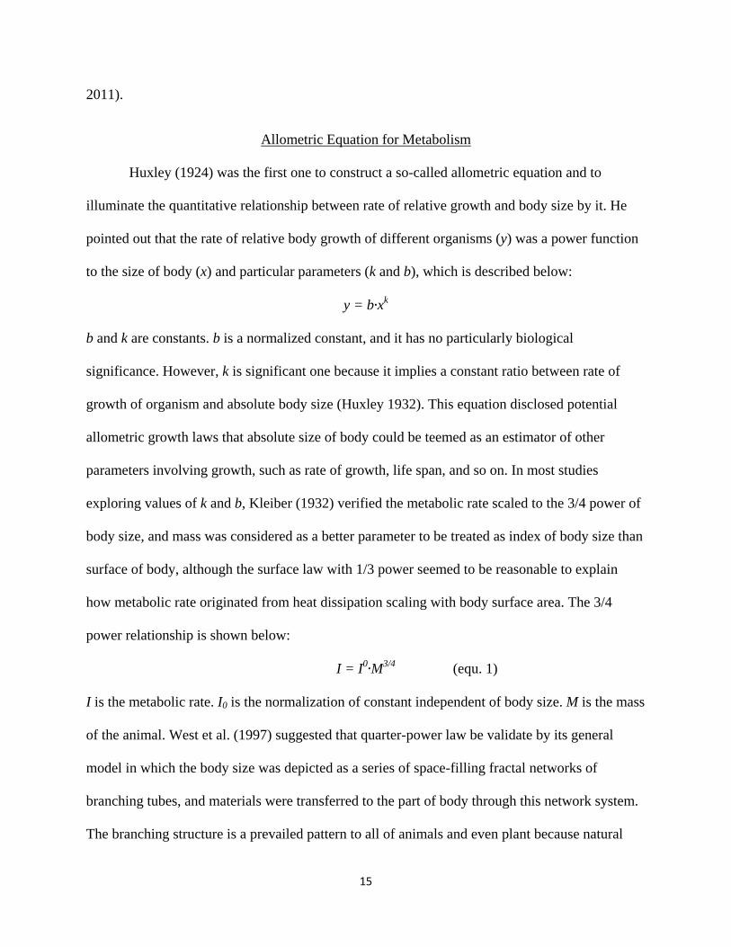
Allometric Equation for Metabolism
Huxley (1924) was the first one to construct a so-called allometric equation and to
illuminate the quantitative relationship between rate of relative growth and body size by it. He
pointed out that the rate of relative body growth of different organisms (y) was a power function
to the size of body (x) and particular parameters (k and b), which is described below:
y = b∙xk
b and k are constants. b is a normalized constant, and it has no particularly biological
significance. However, k is significant one because it implies a constant ratio between rate of
growth of organism and absolute body size (Huxley 1932). This equation disclosed potential
allometric growth laws that absolute size of body could be teemed as an estimator of other
parameters involving growth, such as rate of growth, life span, and so on. In most studies
exploring values of k and b, Kleiber (1932) verified the metabolic rate scaled to the 3/4 power of
body size, and mass was considered as a better parameter to be treated as index of body size than
surface of body, although the surface law with 1/3 power seemed to be reasonable to explain
how metabolic rate originated from heat dissipation scaling with body surface area. The 3/4
power relationship is shown below:
I = I0∙M3/4 (equ. 1)
I is the metabolic rate. I0 is the normalization of constant independent of body size. M is the mass
of the animal. West et al. (1997) suggested that quarter-power law be validate by its general
model in which the body size was depicted as a series of space-filling fractal networks of
branching tubes, and materials were transferred to the part of body through this network system.
The branching structure is a prevailed pattern to all of animals and even plant because natural

16
selection tends to maximize metabolic rate by maximizing exchanging surface and minimizing
distance of fractal networks (West 1997, 1999). Gillooly et al. (2001) suggested some corrections
on the allometric equation to display more details by adding temperature effects. In their
opinions, animal metabolic rate depends on three factors: 1, intensity of reactant, 2, fluxes of
reactants, and 3, kinetic energy of the system. The first two factors are determined by supply and
removal of products. The last factor involves the effect of temperature, which could be quantified
by equation, e-Ei/kT, being used to describes how temperature affects the rate of reactions by
changing molecules’ movement with sufficient kinetic energy. E the activation energy is,
measured in electron volts (1eV=23.06 kcal/mol=96.49 kJ/mol). The relationship between
metabolic rate (B) and temperature (T) is:
𝐵 = 𝐵0(𝑇) ∙ 𝑀34� = 𝐵0 ∙ 𝑀
34� ∙ 𝑒
−𝐸𝑖𝑘𝑇� = 𝐵0(𝑇0) ∙ 𝑀3
4� ∙ 𝑒𝐸𝑖𝑇𝑐
𝑘𝑇𝑇0� (equ. 2) (Gillooly 2001)
B0 is a basal metabolic rate; B is actual metabolic rate; T0 is standard temperature for B0 in k; and
T is the absolute air temperature in K; Tc is difference between T and T0 in K; E is the activation
energy; k is Boltzmann’s constant.
The temperature and mass dependences are also shown in the allometric population
growth model by Savage et al. (2004) in which the population grows under the population
logistic growth law and individual metabolic rules. By applying the Euler integration, the way
temperature, mass, and time scale play their influences was clarified into the equation:
0 00
0 1
( , , ) [(1 ) ]popE BB M T t r ES r
= + + (equ. 3) (Savage et al. 2004)
E0 is a normalization of activation energy; S0 is a constant of mortality rate; B0 is a basal
metabolic rate; r1 is a taxon- and environment-dependent normalization constant. All of these
variables are temperature and mass independent. The population growth rate was just controlled

17
by population metabolic rate regarding with total mass of population, temperature, and time.
Models described above are also extended to predict the allometries of ontogenetic growth
trajectories (West 2001) and other life-history attributes (Savage et al. 2004) that display the
prevalence of allometric equation to explain biological processes in various hierarchies.
The Significance of Ant Workers in Population and Energy Dynamics of Ant Colony
Like the life cycle of the individual ant, the life cycle of an ant colony can be
conveniently divided into three parts: founding stage, ergonomic stage, and reproductive stage
(Hölldobler and Wilson 1990, 143 p). In ergonomic stage, over the weeks and months the
population of workers grows, the average size of the workers increases, and new physical castes
are sometimes added (Hölldobler and Wilson 1990, 143 p). Among the key life history traits of
social insects, the nutritional storage of colonies in response to spatial and temporal variation has
been of considerable interest (Kondoh 1968; Wilson 1974; Rissing 1984; Hasegawa 1993). In
that colonies in the fall season store nutrients in the form of workers’ fats that can be used during
overwinter periods of food scarcity or seeds collected are stored by workers in the nest (Risch
anf Carroll 1986), the size and population of the workers become significant index to estimate
ant colony dynamic. In the seasonal dynamic change of colony size and population, there has
been some evidence that incipient colonies are monomorphic and consist of small workers only,
but as colonies grow, production of larger workers causes the size-frequency distributions to
become strongly skewed. Kaspari (2005) found ants altered colony mass by independently
changing worker mass and/or worker number. It was found that energetic efficiency in
polymorphic colonies (multiple workers cast) was approximately 10% higher than in colonies
composed of only small workers (Porter and Tschinkel 1985). And relying on worker’s
metabolic rate parameters, it is feasible to monitor the colony energy dynamic status. For

18
example, the colony VO2 (oxygen consumption rate) could be accurately estimated from
individual VO2 (Lighton 1989). In 3 species of Pogonomyrmex Harvester Ants, respiration of the
workers was estimated to account for 84-92% of energy assimilated by colony nest (MacKay
1985). Specially, the Damuth’s Rule shows that for large compilations of population densities,
the relationship between the average mass of a species and its average density is generally well
fit to a power function, which enforces the significance of worker size in ant colony (White
2007). Therefore, it is meaningful to test ant colony energy and population dynamics based on
individual worker’s metabolic process influenced by seasonal changes of temperature and food
supply.
The aim of the study reported herein was to investigate ant colonies’ energy and
population dynamics in response to changes of temperature and food. These variables were
simulated under different levels of temperature and food to determine ant colonies’ response to
changes in the environment. Apart from energy and population dynamics, the study also focused
on the effects of temperature on workers’ size, immature ants’ development, and queen’s
reproduction. This study tested the following hypotheses:
H0…there is no effects of temperature and food on ant colony’s energy and population
dynamics.
H1…temperature elevations will increase the risk of ant colonies for dying out because
they need to consume more energy to sustain themselves.
H2…Changes of food availability will affect energy and population dynamics of ant
colonies. Rich food sources can protect ant colonies from decaying even in very high
temperature.

19
CHAPTER 2
MATERIALS AND METHODS
The ant colony energy dynamic ABM model was constructed on the platform of Netlogo
5.0.4.
Purpose
The goal of the model is to simulate the long-term dynamics of an ant colony, especially
focusing on foraging and colony growth. The behavior of individual ants is based on simple rules,
and their behavior is linked to a simple energy flow from the environment to the colony and
metabolism (metabolic equations). The main idea of the model is to apply MTE (Metabolic
Theory of Ecology) to the ant colony to quantify the effects of temperature on the dynamics of
ant colony and to analyze possible scenarios of temperature fluctuations caused by climate
change.
State Variables and Scales
This model is comprised of several parts: individuals, interaction networks, nest, and
environment. The first 2 are modeled explicitly and the last 2 are modeled abstractly. Individual
agents spend time behaving and interacting in the simulation environment. We assume that the
growth of the ant colony is determined by the queen’s fecundity and workers’ efficiency. For
simplification, all stages of offsprings are merged into one state of the “immature ant” agent.
This model starts with a situation that the colony has been initiated by one queen with a varying
number of immature ants, nurses, and foragers. In the model the “immature ants” are produced
by queen at random locations in the nest. The immature ones can develop into nurses or foragers.
The life spans of immature ants and adult workers are the functions of expected longevity,

20
temperature, mass, and energy. We assume that only 2 castes exist in the ant colony, foragers and
nurses. Foragers work in searching for food outside the nest. They find food resources by
random walking or following trail pheromone (Hölldobler and Wilson 1990, 228 p). Nurses feed
immature ants and the queen inside the nest. There has been quantitative evidences that rate of
the trophallaxis (number of workers/hour feeding a larva) varies with the individual larval size
and hunger cues (Cassill 1995, 1999). These relationships strongly suggest that nurses orient
toward queen’s or immature ants’ hunger pheromone. Although workers have different size and
behavioral preferences, these 2 castes, foragers and nurses, can switch jobs depending on
environment (Gordon 2010, 30 p).
The individuals are characterized by state variables: identity number, task assignments,
and internal state (velocity, mass, energy, metabolic rate, and longevity) (Table 1). Workers are
represented by mobile agents: nurses feed immature ants and queen inside the nest; foragers
forage outside the nest. Both of them move at a velocity, v. In the model tasks of workers emerge
from interactions with others agents and environment. The queen is modeled as a motionless
agent who monopolizes some space in the nest. Her tasks are designed to convert the food into
energy and consume energy to live and produce immature ants. Immature ant agents are installed
as immobile agents in the nest as well. They consume energy to support their growth until they
develop into foragers or nurses. Both queen and immature ants release the hunger pheromone to
inform nurses when they are hungry and where they are.
In this model environmental variables are recorded on every step, including intensity of
pheromones, diffusing/evaporating rate of pheromones, and amount of food, time, and
temperature (Table 1). All of these variables are taken into account in workers’ decision-making.
According to the MTE (metabolic theory of ecology), however, metabolic rate and speed will be
21
a function of temperature (described below).
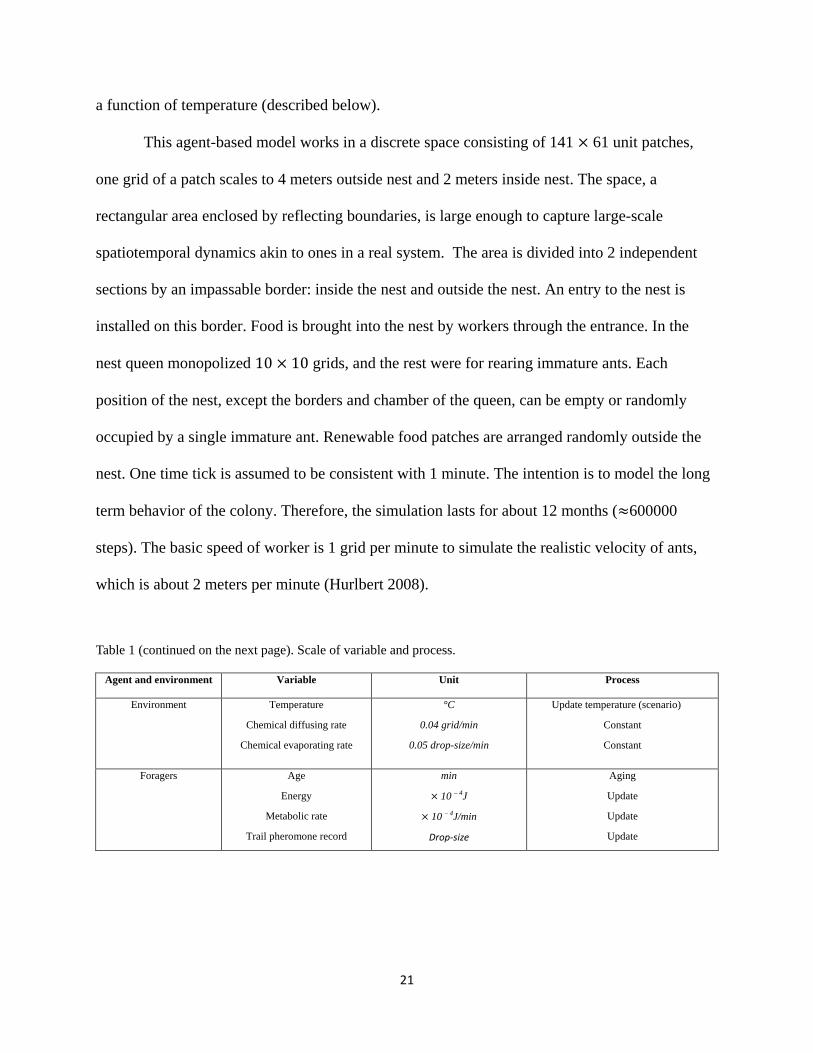
This agent-based model works in a discrete space consisting of 141 × 61 unit patches,
one grid of a patch scales to 4 meters outside nest and 2 meters inside nest. The space, a
rectangular area enclosed by reflecting boundaries, is large enough to capture large-scale
spatiotemporal dynamics akin to ones in a real system. The area is divided into 2 independent
sections by an impassable border: inside the nest and outside the nest. An entry to the nest is
installed on this border. Food is brought into the nest by workers through the entrance. In the
nest queen monopolized 10 × 10 grids, and the rest were for rearing immature ants. Each
position of the nest, except the borders and chamber of the queen, can be empty or randomly
occupied by a single immature ant. Renewable food patches are arranged randomly outside the
nest. One time tick is assumed to be consistent with 1 minute. The intention is to model the long
term behavior of the colony. Therefore, the simulation lasts for about 12 months (≈600000
steps). The basic speed of worker is 1 grid per minute to simulate the realistic velocity of ants,
which is about 2 meters per minute (Hurlbert 2008).
Table 1 (continued on the next page). Scale of variable and process.
Agent and environment Variable Unit Process
Environment Temperature
Chemical diffusing rate
Chemical evaporating rate
°C
0.04 grid/min
0.05 drop-size/min
Update temperature (scenario)
Constant
Constant
Foragers Age
Energy
Metabolic rate
Trail pheromone record
min
× 10 – 4J
× 10 – 4J/min
Drop-size
Aging
Update
Update
Update

22
Table 1 (continued). Scale of variable and process.
Agent and environment Variable Unit Process
Nurses Age
Energy
Metabolic rate
Trail pheromone record
min
× 10 – 4J
× 10 – 4J/min
Drop-size
Aging
Update
Update
Update
Queen Age
Energy
Metabolic rate
Hunger pheromone record
min
× 10 – 4J
× 10 – 4J/min
Drop-size
Aging
Update
Update
Update
Larva Age
Energy
Metabolic rate
Hunger pheromone record
min
× 10 – 4J
× 10 – 4J/min
Drop-size
Aging
Update
Update
Update
Process Overview and Scheduling
At each discrete time step, various agents have series of behaviors to perform in a
sequential order. Foragers patrol outside the nest, constantly detecting a gradient of trail
pheromone; they stop at food sources to carry one mg food (Josens 1998) and return to the nest,
depositing a trail pheromone in the way they passed. They put down food in the nest and repeat
the process or switch to the role of nurse. Carrying 0.002 mg food (Appendix 4) nurses wander
around randomly in the nest. When the nurse locates the hungry queen or immature ant by a
gradient of hunger pheromones, it will move to the target grid cell, put down the food, and feed
the hungry agent. After finishing, it returns to the food storage. This procedure is also repeated
unless it switches to the role of forager. The queen releases the hunger pheromone when her
energy is lower than the critical threshold. The immature ants also release hunger pheromone
when their energy drops below the energy threshold. They develop into workers when their mass
is higher than mass threshold. The behaviors of agents are shown below (Fig.1).

23
a (colony view):
b (queen):
Figure 1 (continued on the next pages). Process of overview of the model. Each task group has a working cycle. a is a colony view, b is a forager.

24
c (immature ant):
d (forager):
Figure 1 (continued). Process of overview of the model. Each task group has a working cycle. c is a nurse, d is an immature ant.

25
e (nurse):
e
Figure 1 (continued). Process of overview of the model. Each task group has a working cycle. e is a queen.

26
f (mass & energy networks of agents):
Figure 1 (continued). Process of overview of the model. Each task group has a working cycle. f is energy-mass conversion.
Design Concepts
Emergence
The equilibriums of worker castes, worker’s population, energy, and mass dynamics
emerge from the individuals’ behavior and metabolism, but the behavior and metabolism are
entirely described by simple empirical and stochastic rules. The balance between foraging
efficiency and feeding efficiency also emerge dynamically from colony needs and prey and food
availability. Reproduction and development speed is the function of fulfilling the nutrition need

27
of the queen and immature ants.
Adaptation and Fitness
Adaptation and fitness are not explicitly included in this model. The only exception is in
the workers’ decision whether the foraging strategy or feeding strategy will be taken. The
decision is based on the amount of food stored in the nest.
Sensing
Individuals are assumed to know their own inner state (energy, mass, age, and
assignments) and behave accordingly. Ants’ sensing mainly depends on smelling and tactile
sensation. The use of visual signals in ants is very minor, and there is no a single example to be
solidly documented (Hölldobler and Wilson 1990, 259 p). Therefore, we assumed ants can sense
their neighbors by close antenna touching. Workers have 2 sensing antennas to perceive
directional signals (Hölldobler and Wilson 1990, 271 p). We assume they wiggle and orient
along varying-concentration odor trail by antennae detection (from right 35oto left 35o). In this
model the workers can diagnose the gradients of pheromone diffused in patches. Cassill (1999)
suggested the ant queen and immatures may release hunger pheromone to notify workers about
their hunger status, akin to the behavior of the brood of honeybees (Fewell 2003). Workers can
also recognize the saturation of food storage. ( Reyes-López 2002) and distinguish dead larvae
from living ones (Robinson et al. 1974).
Interactions
Interactions between different agents are modeled with more details described in the
submodel section. Individuals direct interactions happen when workers feed hungry queen or
immature ants and when workers move dead immature ants to food storage. The saturations of

28
immature ants and queen could also influence the tasks’ switching decisions of workers, but
those influences are not represented as explicit interactions between particular individuals. The
state variables and behaviors of ant agents are also affected by environmental factors. The
temperature is the primary environmental factor to regulate ants’ moving velocity and
metabolism. Ants tend to move faster and consume more energy in high temperature than ants in
low one. Accordingly, workers are designed to have daily rhythm of temperature preference.
In this model workers can’t cross the reflecting walls and borders. When they reach the
borders and walls, they will redirect randomly. The environment is also changed by ants. The
amount of the pheromones deposited in the grid will decay unless ants lay new ones. The food
will be reallocated from food sources to food storage by foraging and transporting of workers.
Stochasticity
Random numbers were generated to simulate the realistic process by using the netlogo
built in random generator. The following state and environment variables are stochastic: initial
location, walking direction, developmental orientation of immature ants, and amount of food per
patch. We assume the initial energy of ants, initial number of ants, initial mass of ants, initial age
of workers, and initial amount of food in the food sources and storage distributed normally. In
the model ants make decisions by possibility that could be quantified in a normal cumulative
distribution functions (𝜇 = 𝑡ℎ𝑟𝑒𝑠ℎ𝑜𝑙𝑑, 𝜎 = 1).
Collectives
Collectives are represented in the model as task groups of workers, namely adult ants are
either nurses or foragers. However, these collectives emerge in nature because in the model
workers can switch their tasks freely by interacting with others and environment.

29
Observation
In this model Netlogo offers a visual platform to monitor the behavior of the system. The
monitor is used for inspecting and testing the model step by step. The following parameters are
monitored and saved into a file for further analyzes: the population size of the ant colony,
number of nurses, number of foragers, number of immature ants, total energy of the ant colony,
total mass of the ant colony, amount of food stored, birth rate, growth rate of immature ants,
death rate of immature and adult ants, foraging efficiency, feeding efficiency, developing time of
immature ants, age structure of the ant colony, temperature of the nest, and temperature of the
environment. To test our hypotheses and compare the predictions, Kruskal-Wallis test in SPSS
Statistical Package (Version 19) was used.
Initialization
The initial parameters in the model are listed in the Table 2. The simulations were
repeated 10 times so as to consider the variability between outputs for the same set of parameters
and initial conditions. The variability came from the stochasticity in the processing of the model.
The onset of the ant colony imitated the start of a natural colony after the workforce of the
colony reached 200. In this stage the queen and Nimmature ant live in the nest and Nnurses work inside
the nest to feed the queen and immature ants. Nforagers work outside the nest to forage. There is
one cluster of food patches arranged randomly outside the nest. And 35 mg food is stored in the
nest. Before the model starts running foragers and nurses are positioned in the environment
randomly.
30
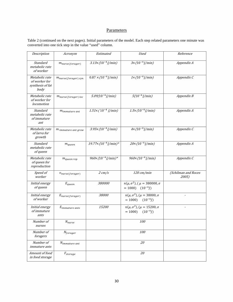
Parameters
Table 2 (continued on the next pages). Initial parameters of the model. Each step related parameters one minute was converted into one tick step in the value “used” column.
Description Acronym Estimated Used Reference
Standard metabolic rate
of worker
𝑚𝑛𝑑𝑒𝑑𝑑(𝑑𝑒𝑒𝑒𝑓𝑑𝑒) 3.13×(10−4J/min) 3×(10−4J/min) Appendix A
Metabolic rate of worker for
synthesis of fat body
𝑚𝑛𝑑𝑒𝑑𝑑(𝑑𝑒𝑒𝑒𝑓𝑑𝑒) 𝑑𝑦𝑛 0.87 ×(10−4J/min) 1×(10−4J/min) Appendix C
Metabolic rate of worker for locomotion
𝑚𝑛𝑑𝑒𝑑𝑑(𝑑𝑒𝑒𝑒𝑓𝑑𝑒) 𝑡𝑒𝑙 5.09(10−4J/min) 5(10−4J/min) Appendix B
Standard metabolic rate of immature
ant
𝑚𝑑𝑙𝑙𝑒𝑒𝑑𝑒𝑑 𝑒𝑛𝑒 1.51×( 10−4 J/min) 1.5×(10−4J/min) Appendix A
Metabolic rate of larva for
growth
𝑚 𝑑𝑙𝑙𝑒𝑒𝑑𝑒𝑑 𝑒𝑛𝑒 𝑓𝑒𝑒𝑔 3.95×(10−4J/min) 4×(10−4J/min) Appendix C
Standard metabolic rate
of queen
𝑚𝑞𝑑𝑑𝑑𝑛 19.77×(10−4J/min)* 20×(10−4J/min) Appendix A
Metabolic rate of queen for
reproduction
𝑚𝑞𝑑𝑑𝑑𝑛 𝑒𝑑𝑒 960×(10−4J/min)* 960×(10−4J/min) Appendix C
Speed of worker
𝑣𝑛𝑑𝑒𝑑𝑑(𝑑𝑒𝑒𝑒𝑓𝑑𝑒) 2 cm/s 120 cm/min (Schilman and Roces 2005)
Initial energy of queen
𝐸𝑞𝑑𝑑𝑑𝑛 380000 𝑛(𝜇,𝜎2), ( 𝜇 = 380000,𝜎= 1000) (10−4𝐽)
Initial energy of worker
𝐸𝑛𝑑𝑒𝑑𝑑(𝑑𝑒𝑒𝑒𝑓𝑑𝑒) 38000 𝑛(𝜇,𝜎2), (𝜇 = 38000,𝜎= 1000) (10−4𝐽)
-
Initial energy of immature
ants
𝐸𝑑𝑙𝑙𝑒𝑒𝑑𝑒𝑑 𝑒𝑛𝑒𝑑 15200 𝑛(𝜇,𝜎2), (𝜇 = 15200,𝜎= 1000) (10−4𝐽)
-
Number of nurses
𝑁𝑛𝑑𝑒𝑑𝑑 100
Number of foragers
𝑁𝑑𝑒𝑒𝑒𝑓𝑑𝑒 100
Number of immature ants
𝑁𝑑𝑙𝑙𝑒𝑒𝑑𝑒𝑑 𝑒𝑛𝑒 20
Amount of food in food storage
𝐹𝑑𝑒𝑒𝑒𝑒𝑓𝑑 20

31
Table 2 (continued). Initial parameters of the model. Each step related parameters one minute was converted into one tick step in the value “used” column.
Description Acronym Estimated Used Reference
Threshold of food storage saturation
FStoreThreshold 𝑛(𝜇,𝜎2), (𝜇 = 30,𝜎= 10) (10−4𝐽)
Initial mass of worker
𝑀𝑛𝑑𝑒𝑑𝑑(𝑑𝑒𝑒𝑒𝑓𝑑𝑒) 2 mg 𝑛(𝜇,𝜎2), (𝜇 = 2,𝜎= 0.05) (𝑚𝑔)
(Jensen 1978)
Initial mass of immature ants
𝑀𝑡𝑑𝑙𝑙𝑒𝑒𝑑𝑒𝑑 𝑒𝑛𝑒 0.8mg 𝑛(𝜇,𝜎2), (𝜇 = 0.8,𝜎= 0.2) (𝑚𝑔)
(Brian 1973)
Initial mass of queen
𝑀𝑞𝑑𝑑𝑑𝑛 2~80 mg 20 mg (Tschinkel 1978; Keller
1989) Initial age of
worker Aage 𝑛(𝜇,𝜎2), (𝜇
= 10000, 𝜎= 2000)
Expected longevity of
nurses (foragers)
𝐴𝑒𝑓𝑑������ 190080 190080
Diffusing rate of hunger
pheromone
𝑟 ℎ𝑑𝑛𝑓𝑑𝑒 𝑑𝑑𝑑𝑑𝑑𝑑𝑑 0.046
Evaporation rate of hunger
pheromone
𝑟 ℎ𝑑𝑛𝑓𝑑𝑒 𝑑𝑒𝑒𝑒𝑒𝑒𝑒𝑒𝑑 0.052
Diffusing rate of trail pheromone
𝑟𝑒𝑒𝑒𝑑𝑡 𝑑𝑑𝑑𝑑𝑑𝑑𝑑 0.04
Evaporation rate of evaporate pheromone
𝑟𝑒𝑒𝑒𝑑𝑡 𝑑𝑒𝑒𝑒𝑒𝑒𝑒𝑒𝑑 0.05
Amount of food at each food patch
F 𝑛(𝜇,𝜎2), (𝜇 = 225,𝜎= 50) (𝑓𝑜𝑜𝑑 𝑢𝑛𝑖𝑡)
Antenna sensing angle
A 70 70
Catabolism weight-energy
conversion factor
c’ 19.02J/mg 190000(10−4)𝐽/𝑚𝑔 (Cummins and
Wuycheck 1971; Hou et
al. 2008)
Anabolism weight-energy conversion
factor
c >19.02J/mg 200000(10−4)𝐽/𝑚𝑔 (Perrin 1995;Kaspari
2005)
Energy threshold of queen for
hunger
Equeen threshold 380000 (10−4)𝐽/𝑚𝑔 (Cummins and
Wuycheck 1971)
Energy threshold of worker for
hunger
Eworker threshold 380000 (10−4)𝐽/𝑚𝑔

32
Table 2 (continued). Initial parameters of the model. Each step related parameters one minute was converted into one tick step in the value “used” column.
Input
In the model the environment was parameterized by daily air temperature of Johnson City,
TN in 2010. The temperature dataset is from National Ocean and Atmosphere Administration
(NOAA) (http://www.ncdc.noaa.gov/cdo-web/). These temperature data was used to construct a
smooth distribution with 1-minute steps to conform the resolution of the model. In the
“experiment of temperature changes”, new temperature data were created by elevating 2, 4, 6, 8,
10, 12, and 14 centigrade to the current temperature data of Johnson City. Because the advantage
of nesting in the soil is the protection provided by the nest against high and low temperature
Description Acronym Estimated Used Reference
Energy threshold of immature ants for
hunger
Eimmature ant threshold 15200 (10−4)𝐽/𝑚𝑔
a ( responding factor of hunger
pheromone gland toward energy
status)
a 5
Mass lower threshold of worker
for dying
MWorkLowerThreshold 1mg
Mass upper threshold of worker
for dying
MWorkUpperThreshold 5mg
Mass threshold of immature ants for
dying
Mimmature ant threshold 0.5mg
Mass of threshold of queen for dying
Mqueen threshold 15mg
One bite of ant Bant 0.023mg
4420(10−4)𝐽
0.02mg
4400(10−4)𝐽
Appendix D
Drop size of trail pheromone
droptrail 180 180
Width of food sources
Wfood 3 patch wide

33
extremes, rain, or wind (Moyano 2013), we assumed the ant colonies nest in the soil. In the
model the colonies could not actively thermo-regulate nest temperature (𝑇𝑛𝑑𝑑𝑒) because of the
small size population of colonies. The nest temperature equated to soil temperature in the 10cm
depth that correlated well with air temperature because both are determined by the energy
balance at the ground surface (Zheng et al. 1993). The soil temperature was regressed to air
temperature (Tair) in equation 4:
𝑇𝑛𝑑𝑑𝑒 = 𝑇𝑑𝑒𝑑𝑡 = 0.89 ∙ 𝑇𝑒𝑑𝑒 + 2.31 euq.4 (Zheng et al. 1993)
We implemented different levels of food with 1, 2, and 3 patch wide per food source patch in the
model to simulate different richness of food sources.
Submodels
The Tasks of Agents
In this model the stationary queen produces all the offsprings labeled “immature ants”.
Immature ants are immobile agents as well, and they finally develop into the forager or nurse
ants. The events of reproduction and development are controlled by mass and energy (in
Reproducing and developing). Foragers leave nest to collect and carry food back to the nest (in
Foraging). Nurses enter into the nest to feed hungry queen or immature ants under directions of
hunger pheromone (in Feeding).
Reproducing and Developing: The mass of queen and immature ants change dynamically
(in Energy and Mass). The event of reproduction or development occurs when queen or
immature ants are heavier than their mass thresholds. The queen lays an egg in a random
nonoccupied position of the nest and this immature ant stays there until it becomes an adult.
When the immature ant becomes a mature one, it will emerge and start work next to the food
storage as the nurse ant or will emerge and start to work next the nest entrance as the forager.

34
Initial decision on the first task is a random process.
Foraging: The foraging task could be viewed as 2 alternating status: start from the nest
and reach the food source, and start from the food source laden with food and reach the nest
(Panait, 2004). In the first status foragers depart nest in search of food by walking forward with
random sniffing angle between left 35o and right 35o or following gradient of trail pheromone
they encountered. Their moving velocity v:
𝑣 = 𝑣0 ∙ 𝑀1/4 ∙ 𝑒−𝐸𝑘
𝑇𝑐𝑖𝑟� (equ. 4) (Hurlbert 2008)
𝑣0 is standard velocity of foragers at 20 ℃; 𝑇𝑒𝑑𝑒 is environment temperature; 𝑀 is the mass of
agent; 𝐸 is the activation energy; 𝑘 is Boltzmann’s constant. In the second status we assume that
foragers are able to navigate to the nest by using the shortest distance after finding the food.
Therefore, the pheromone trail between the food item and the nest is also formed on the shortest
distance between the 2 positions. Foragers bring 1 mg food back to nest directly. When they
come back, food will be stored in the food storage of the nest.
Feeding: Each turn, the nurse keeps motionless and stays very close to queen or immature
ants mouthparts to sweep antenna until larva terminates the feeding and worker move away as
Cassill (1995) described it in fire ant, Solenopsis invicta. In the model feeding is also viewed as 2
alternating status: start from the food storage laden with food and reach the hungry queen or
immature ants, and start from the queen or immature ants and reach the food storage. At the first
status nurses carrying 0.002 mg food (Appendix 4) look for hungry agents in the nest by the
same random walking as forager until they encounter and follow the gradient of hunger
pheromone. Feeding events only happen in hungry agents nurses encounter (Cassill 1995). The
nurses move at velocity v’ described by equation 4 with exposed nest temperature, 𝑇𝑛𝑑𝑑𝑒. When
they reach patches of hungry agents, 0.002 mg food is fed at 1 time-step. At the second status

35
assumedly, nurses can go back to food storage directly.
Dying: Deaths of workers are age-controlled. The age of each individual is monitored.
The expected longevity of worker is about 4.4 months (≈ 190080 steps) (Calabi and Porter 1989),
but it is influenced by temperature and mass as follows:
𝐿 = 𝐿𝑒𝑐𝑝𝑒𝑐𝑡𝑒𝑑𝑀−1 4⁄ ∙𝑑−𝐸 𝑘𝑇⁄ (equ. 5) (Savage et al. 2004)
Where 𝐿 is real longevity; 𝐿𝑑𝑥𝑒𝑑𝑙𝑒𝑑𝑑is expected or average longevity; 𝑀 is the mass of agent; 𝐸 is
the activation energy; 𝑘 is Boltzmann’s constant. We assume their death is the cumulative
function of worker’s longevity probability distribution at 24℃, N(𝜇=190080,𝜎=20000)(min)
( Calabi and Porter 1989). When workers are older than L, their death probability will increase
considerably by death accumulative probability function:
𝐹𝑑𝑑𝑒𝑒ℎ(𝑒) = ∫𝑓𝑡𝑒𝑛𝑓𝑑𝑒𝑑𝑒𝑦(𝑒)𝑑𝑒, (𝜇 = 190080,𝜎 = 20000) (equ. 6)
In another way, when agents starve for a long time, substances such as adipose, protein, and
glycogen will be consumed and converted to the energy for basic energy demands. Therefore, the
mass of agent can stimulate death event when it drops below mass threshold of agent (Table 2).
When death event occurs, agent will be removed from the colony except the dead immature ant
that will be transported into the food storage by workers and part of the dead immature ant (50%)
is reused as food.
Interactions
In terms of hunger pheromone and trail pheromone, pheromone communication is the
primary way to connect ants having no direct interactions. Pheromone chemicals share part of
patch-pheromone concentration (𝑟𝑑𝑑𝑑𝑑𝑑𝑑𝑑) to its 8 neighboring patches. The patch-pheromone
chemicals will decay at an evaporating rate, 𝑟𝑑𝑒𝑒𝑒𝑒𝑒𝑒𝑒𝑑 . In the model foragers deposit trail
pheromone (droptrail) per patch at the patches they passed through after they discover food and

36
get ready to return to nest. Hungry queen and immature ants release hunger pheromone based on
their energy status:
𝐷ℎ𝑑𝑛𝑓𝑑𝑒 𝑒ℎ𝑒𝑒𝑙𝑒𝑛𝑑 = 𝑎 ∙ (𝐸 − 𝐸 𝑒ℎ𝑒𝑑𝑑ℎ𝑒𝑡𝑑) (equ. 7)
𝐷ℎ𝑑𝑛𝑓𝑑𝑒 𝑒ℎ𝑒𝑒𝑙𝑒𝑛𝑑 is the concentration of hunger pheromone of queen or immature ant; 𝐸 is the
energy of queen or immature ant; 𝐸𝑒ℎ𝑒𝑑𝑑ℎ𝑒𝑡𝑑 is the energy threshold of queen or immature ant; a
is responding factor of hunger pheromone gland of queen or immature ant toward energy status.
Outgoing foragers detect the trail pheromone at their neighboring patches within 1 grid distance,
and nurses sense hunger pheromone within 0.5 grid distance (gridoutside nest : gridinside nest = 2:1).
Both of workers can recognize the concentration of pheromone and move along the gradient to
area of high concentration. Workers will change moving directions when they meet the borders
of the environment and nest. The dead immature ants can be recognized and transported to food
storage by workers.
Changing of Tasks
Workers have behavioral flexibility. There are 2 worker tasks in this model, foraging and
nursing. Their tasks allocation depends on the environment and their inner states. Workers can’t
change tasks unless they complete the previous one. In this model forager and nurses need to
decide whether nursing or foraging at every time they finish previous task. Ant workers tend to
change task when more ants are required for particular tasks (Gordon 1989). The harvester ant,
Messor barbarus, was documented to recognize saturation of food storage and modified foraging
strategy based on it (Reyes-López 2002). Therefore, we assume their decisions are based on the
amount of the food stored in the nest. The nursing and foraging tendency are quantified as below:
𝑃𝑛𝑑𝑒𝑑𝑑𝑛𝑓(𝑣; 𝜇,𝜎) = �𝑓(𝑣)𝑑𝑣 , (𝜇 = 20,𝜎 = 5)
𝑃𝑑𝑒𝑒𝑒𝑓𝑑𝑛𝑓 = 1 − 𝑃𝑛𝑑𝑒𝑑𝑑𝑛𝑓 (equ. 8)

37
𝑃𝑛𝑑𝑒𝑑𝑑𝑛𝑓 is the probability to nurse; 𝑃𝑑𝑒𝑒𝑒𝑓𝑑𝑛𝑓 is the probability to forage; 𝑣 is the amount of the
food stored in the nest.
Energy and Mass
Energy, food, and mass are 3 most important variables to regulate agents’ behaviors.
These 3 variables can be quantified and their relationships are described below (Fig.2).
Metabolism includes the catabolic and anabolic processes:
Figure 2. Partitioning of energy assimilated from food.
Agents assimilate energy from food for energy storing (somatic growth and reproduction),
restive maintaining, biosynthesis accumulation for fat body, and locomotion (Hou et al. 2008).
When agents starve, the storage of fat will be consumed to maintain agents’ living (Griffiths
1991). In this model we hypothesized the temperature has no impact on food size selections of
ant, and the constant size of food could be eaten as feeding and eating events occur (Cummins
1971). The constant energy converted from food will be allocated to 2 or 3 partitions for
immature ants, worker, and queen (Fig. 2, 3). Metabolic rate influenced by temperature and mass

38
controls the process of energy-mass conversion. Energy allocation equations are shown below
(equ. 9, 10, 11, 12):
𝑚𝑛𝑑𝑒𝑑𝑑 𝑒𝑒𝑒𝑒𝑡 =(𝑚𝑛𝑑𝑒𝑑𝑑 𝑡𝑒𝑙𝑒𝑙𝑒𝑒𝑑𝑒𝑛+ 𝑚𝑛𝑑𝑒𝑑𝑑 𝑒𝑑𝑑𝑒)∙ 𝑀34� ∙ 𝑒
𝐸𝑖𝑇𝑐𝑘𝑇0� (equ. 9)
𝑚𝑑𝑒𝑒𝑒𝑓𝑑𝑒 𝑒𝑒𝑒𝑒𝑡 =(𝑚𝑑𝑒𝑒𝑒𝑓𝑑𝑒 𝑡𝑒𝑙𝑒𝑙𝑒𝑒𝑑𝑒𝑛+ 𝑚𝑑𝑒𝑒𝑒𝑓𝑑𝑒 𝑒𝑑𝑑𝑒)∙ 𝑀34� ∙ 𝑒
𝐸𝑖𝑇𝑐𝑘𝑇0� (equ. 10)
𝑚𝑑𝑙𝑙𝑒𝑒𝑒𝑑𝑒𝑑 𝑒𝑛𝑒 𝑒𝑒𝑒𝑒𝑡=(𝑚𝑑𝑙𝑙𝑒𝑒𝑒𝑑𝑒𝑑 𝑒𝑛𝑒 𝑒𝑑𝑑𝑒+𝑚𝑑𝑙𝑙𝑒𝑒𝑒𝑑𝑒𝑑 𝑒𝑛𝑒 𝑓𝑒𝑒𝑔) ∙ 𝑀34� ∙ 𝑒
𝐸𝑖𝑇𝑐𝑘𝑇0� (equ. 11)
𝑚𝑞𝑑𝑑𝑑𝑛 𝑒𝑒𝑒𝑒𝑡=(𝑚𝑞𝑑𝑑𝑑𝑛 𝑒𝑑𝑑𝑒 + 𝑚𝑞𝑑𝑑𝑑𝑛 𝑒𝑑𝑒𝑒𝑒𝑑𝑑𝑙𝑒𝑑𝑒𝑛) ∙ 𝑀34� ∙ 𝑒
𝐸𝑖𝑇𝑐𝑘𝑇0� (equ. 12)
Known as anabolism, energy is preserved for somatic growth per step by equation 13, 14
(Gillooly et al. 2001; Hou et al. 2008):
𝑆 = 𝐸𝑙 ∙𝑑𝑙𝑑𝑒
(equ. 13)
From these we derived:
∆𝑚 = 𝑑𝑙𝑑𝑒
= 𝑆𝐸𝑐
= 𝑙𝑠𝑦𝑛
𝑙∙𝑀3 4� ∙𝑑
𝐸𝑇𝑘𝑇0�
(equ. 14)
Where ∆𝑚 is a fact body accumulation rate; S is rate of energy stored; Ec is the energy content of
biomass; 𝑚 𝑑𝑒𝑒𝑒𝑑𝑛𝑓 is the energy for storing fat body per step; c is anabolism factor; 𝑀 is the
mass of agent; 𝐸 is the activation energy; 𝑘 is Boltzmann’s constant; T0 is standard temperature
20℃.
When the agents starve, catabolism became larger and it elicits energy loss (Perrin 1995).
The fat body will be consumed to maintain basic energy requirement (equ. 15), which causes
weight loss:
∆𝑚′ = 𝑑𝑙′𝑑𝑒
= 𝑙𝑟𝑒𝑠𝑡+𝑙𝑙𝑜𝑐𝑜𝑐𝑜𝑡𝑖𝑜𝑛
𝑙′∙𝑀3 4� ∙𝑑
𝐸𝑖𝑇𝑐𝑘𝑇0�
(equ. 15)
∆𝑚′ is a mass loss rate, c’ is catabolism factor.

39
Monitored Values
The number of agents belonging to different groups, age structure, total energy, and mass
of ant colony are followed and calculated. When forager or nurses finish their previous tasks, the
working efficiency is calculated every step as follow (equ. 16):
𝑟𝑑𝑒𝑒𝑒𝑓𝑑𝑛𝑓 = ∑ 𝐹𝑓𝑖𝑖0
𝑛𝑓𝑜𝑟𝑐𝑔𝑒𝑟+𝑛𝑛𝑢𝑟𝑠𝑒, 𝑟𝑛𝑑𝑒𝑑𝑑𝑛𝑓 = ∑ 𝐹𝑑𝑖𝑖
0𝑛𝑓𝑜𝑟𝑐𝑔𝑒𝑟+𝑛𝑛𝑢𝑟𝑠𝑒
𝐹𝑔 = � 0 (𝑓𝑜𝑟𝑎𝑔𝑖𝑛𝑔 𝑖𝑛𝑐𝑜𝑚𝑒𝑙𝑒𝑡𝑒 𝑒𝑒𝑟 𝑠𝑡𝑒𝑒)1 (𝑓𝑜𝑟𝑎𝑔𝑖𝑛𝑔 𝑐𝑜𝑚𝑒𝑙𝑒𝑡𝑒 𝑒𝑒𝑟 𝑠𝑡𝑒𝑒)
𝐹𝑑 = � 0 (𝑛𝑢𝑟𝑠𝑖𝑛𝑔 𝑖𝑛𝑐𝑜𝑚𝑒𝑙𝑒𝑡𝑒 𝑒𝑒𝑟 𝑠𝑡𝑒𝑒)1 (𝑛𝑢𝑟𝑠𝑖𝑛𝑔 𝑐𝑜𝑚𝑒𝑙𝑒𝑡𝑒 𝑒𝑒𝑟 𝑠𝑡𝑒𝑒) (equ.16)
i is index of workers. During each run the birth rate, death rate, and growth rate of population are
calculated by equ. 17, 18, 9, 20:
𝑟𝑓𝑒𝑒𝑔𝑒ℎ =∑ 𝑛𝑡(𝑛𝑒𝑤 𝑤𝑜𝑟𝑘𝑒𝑟𝑠)𝑡0
𝑒 (equ. 17)
𝑟𝑏𝑑𝑒𝑒ℎ =∑ 𝑛𝑡(𝑛𝑒𝑤 𝑖𝑐𝑐𝑐𝑡𝑢𝑟𝑒 𝑐𝑛𝑡𝑠)𝑡0
𝑒 (equ. 18)
𝑟𝑔𝑒𝑒𝑘𝑑𝑒 𝑑𝑑𝑒𝑒ℎ =∑ 𝑛𝑡(𝑑𝑒𝑐𝑑 𝑤𝑜𝑟𝑘𝑒𝑟𝑠)𝑡0
𝑒 (equ. 19)
𝑟𝑑𝑙𝑙𝑒𝑒𝑑𝑒𝑑 𝑑𝑑𝑒𝑒ℎ =∑ 𝑛𝑡(𝑑𝑒𝑐𝑑 𝑖𝑐𝑐𝑐𝑡𝑢𝑟𝑒 𝑐𝑛𝑡)𝑡0
𝑒 (equ. 20)
t is the number of steps, nt(new 𝑔𝑒𝑒𝑘𝑑𝑒𝑑)is the number of new workers at the t-th step,
nt(𝑛𝑑𝑔 𝑑𝑙𝑙𝑒𝑒𝑑𝑒𝑑 𝑒𝑛𝑒𝑑)is the number of new immature ants at the t-th step, nt(new forager)is the
number of forager at the t-th step, nt(𝑑𝑑𝑒𝑑 𝑔𝑒𝑒𝑘𝑑𝑒𝑑)is the number of dead workers at the t-th
step, 𝑛𝑡(𝑑𝑒𝑎𝑑 𝑖𝑚𝑚𝑎𝑡𝑢𝑟𝑒 𝑎𝑛𝑡) is the number of dead immature ants a the t-th step. The average
developmental time of immature ants is recorded based on every individual that has developed.
The average developmental time of immature ants is calculated by equ. 21:
𝑡𝑑𝑑𝑒𝑑𝑡𝑒𝑒𝑙𝑑𝑛𝑒 = ∑ 𝑒 𝑖𝑖0
𝑛𝑑𝑒𝑣𝑒𝑙𝑜𝑝𝑒𝑑 (equ. 21)
i is index of new adult worker. 𝑡𝑑𝑑𝑒𝑑𝑡𝑒𝑒𝑙𝑑𝑛𝑒 is an average developmental time of the new adult

40
worker, 𝑡 𝑑 is the developmental time of new adult worker i, 𝑛𝑑𝑑𝑒𝑑𝑡𝑒𝑒𝑑𝑑 is the number of new
adult workers. In order to compare the energy consumption, the hungry rate was monitored by
equ. 22:
𝑅ℎ𝑑𝑛𝑓𝑑𝑒 =∑ 𝑛𝑡(ℎ𝑢𝑛𝑔𝑟𝑦 𝑒𝑣𝑒𝑛𝑡𝑠)𝑡0 𝑇⁄
∑ 𝑛𝑡(𝑤𝑜𝑟𝑘𝑒𝑟)𝑡0
�������������������� (equ. 22)
Where t is the number of steps, T is the time of simulation, nt(hungry events) is the total number of
hungry events in workers at the t-th step, ∑ 𝑛𝑒(𝑔𝑒𝑒𝑘𝑑𝑒)𝑒0
���������������� is the average number of workers per
step.
Experiment
We did 3 experiments to test temperature and food’s impacts on ant colonies.
Experiment of Temperature Changes
Constant Temperature vs. Dynamic Temperature: In the constant temperature treatment,
the model started with the mean temperature in Johnson City 2010, 13.5oC, and the nest
temperature was estimated to be 14.3oC (equ. 4). In the dynamic temperature treatment, the daily
temperature of Johnson City, TN, in 2010 was parameterized into the model to manipulate
dynamic air temperature (maximum 29.15oC, minimum -9.5oC, mean 13oC). Every simulation
ran for 516 781 steps (≈ 359 days). In every treatment, 20 parallel simulations were run to
estimate statistically.
Different Elevated Temperature Regimes: Based on daily air temperature record in
Johnson City TN in 2010, we set up 8 treatments to manipulate elevated temperature regimes:
+0oC, +2oC, +4oC, +6oC, +8oC, +10oC, +12oC, and +14oC. Each simulation starts with
parameters in Table 2 and ran for 516 781 steps (≈ 359 days). In every treatment, 20 parallel
simulations were run to estimate statistically.

41
Experiment of Food Availability Changes
In this experiment we estimated the food availability based on the width of food patches. Three
levels of food richness were implemented into the model: 2 patch wide food sources, 3 patch wide food
sources, and 5 patch wide food sources. Each simulation started with temperature of Johnson City in 2010,
and ran for 516 781 steps (≈ 359 days). In every treatment 20 parallel simulations were run to estimate
statistically.
Experiment of Climate Changes
In order to simulate climate changes in terms of high temperature and food richness, we
inserted high food availability and temperature into the model together. The model started with
temperature elevated 14oC regime (maximum: 37oC; minimum: 15oC; mean: 27oC). Two levels
of food availability were manipulated: 3-patch wide food sources as the control and 5-patch wide
food as the treatment. Every simulation ran for 516 781 steps (≈ 359 days). In this treatment 20
parallel simulations were run to estimate statistically.

42
CHAPTER 3
RESULTS
Effects of Seasonal Temperature Change on Population and Energy Dynamic of Ant Colony
The colonies started with the daily temperature in Johnson City TN in 2010 as the
dynamic temperature simulation (TJohnsonCity: maximum 23oC, minimum 1oC, mean 13oC) or with
13oC as constant temperature simulation. In single simulation with dynamic temperature, the
population size endured 4 stages during the whole year: it shrunk significantly during spring,
increased in summer, stabilized in autumn, and declined again in winter (Fig. 3a). Comparing
population size distribution to annual temperature (Fig. 3a), we can conclude that temperature-
dependent population size keeps growing during the summer until the size of colony arrives at a
maximum in the middle of the autumn. Afterwards, the population of colony declines till middle
of the spring. In addition, the colony size increases above about 12.5oC and decreases below
about 12.5oC. The 𝑟𝑑𝑒𝑒𝑒𝑓𝑑𝑛𝑓 (number of times becoming hungry per worker per minute, equ. 22),
the average foraging efficiency of worker (Times of a resource-laden ant returning to the nest per
worker per min, equ. 16) and average mass of workers varies seasonally as well (Fig. 3c, d).
Differently, the colonies simulated with the constant temperature (13oC) have no apparent
declining stages, and its size grows in logistic manner (Fig.3b).

43
a:
b:
c:
Figure 3 (continued on the next page). Population dynamics in single simulations: (a) Daily temperature in Johnson City TN 2010 (red line); modeled population size of colonies (blue line); (b) Constant temperature (red line); population size of colonies (blue line); (c) Foraging efficiency of workers in dynamic T.
-0.1
0.1
0.3
0.5
0.7
0 100 200 300 400
Fora
ging
effi
cien
cy
(No.
fora
ging
s / p
er w
orke
r. pe
r m
in)
Time (days)

44
d:
Figure 3 (continued). Population dynamics in single simulations: (d) Average mass of workers in dynamic temperature.
We find the dynamic temperature tends to make more fluctuations in energy, population
size of colonies, and foraging efficiency of workers than what constant temperature does (Fig. 4a,
b, d). The food storage consumed more extensively in the dynamic temperature than in constant
temperature during the summer (Fig.4c).
a: b:
Figure 4 (continued on the next page). Average value of 20 parallel simulations with constant temperature (red line) and dynamic temperature (blue line): (a) energy of ant colony; (b) population size of ant colony.

45
c: d:
Figure 4 (continued). Average value of 20 parallel simulations with constant temperature (red line) and dynamic temperature (blue line): (c) food storage in the nest; and (d) foraging efficiency of workers.
Effects of Temperature Elevations on Population and Energy Dynamic of the Ant Colony
The resistance of the colonies to elevated temperature regimes is fairly robust. Only 12.5%
colonies died out at the end of year. The rest of the experimental modeled colonies could
stabilize their colony’s size and energy levels (Fig.5a-b). We used 270th day as a time point for
comparison, given that this time is the transition of summer to autumn. On the 270th day, the
differences of energy and population among 8 temperature elevation regimes were tested in
pairwise test if the Kruskal-Wallis test showed that the groups in fact have not the same median
(N=159, d.f. = 7). We detected the significant differences in the energy level of the colony
between 0oC and 4 oC (p < 0.05), 4 oC and 8 oC (p < 0.001) and 8 oC and 12 oC (p < 0.05) to
indicate that the energy of colonies tend to increase as temperature has small elevations (≤4oC),
and decline in the higher elevated temperature regimes (≥6oC) (Fig. 5c-d). The dynamic of
colonies’ size has the same pattern as we described for the energy. There are significant
differences between 0oC and 4 oC (p < 0.05), 4 oC and 8 oC (p < 0.001), and 8 oC and 14 oC (p <
0.001).

46
a: b:
c: d:
Figure 5. Effects of temperature elevation regime on (a) energy of colonies, (b) population size of colonies, (c) energy of colonies on the 270th day, and (d) average population of colonies on the 270th day. p-value based on pairwise test using the Kruskal-Wallis test (N=159, d.f.=7).
In the cases of extreme high temperatures, the colonies died out because of food shortage
or/and low birth rate of immature ants (Figs.6, 7). The average birth rate of immature ants in 6oC
elevations is significantly higher than in 0oC (Kruskal-Wallis pairwise test, p < 0.001, N=160,
d.f.=7), and the rate in 12oC elevation is significantly lower than in 6oC elevation (Kruskal-
Wallis pairwise test, p < 0.001, N=160, d.f.=7). Furthermore, there are no significant differences
of birth rate among 4oC, 6oC, 8oC, and 10oC elevations. Those results reveal that the birth rates
of workers respond to temperature in the manner of a single-peak (Fig.7).

47
a: b:
c: d:
Figure 6. Two cases of colony extinction at the 14oC elevated temperature regime: (a) and (c) energy of colony; (b) and (d) food storage in nest.
Figure 7. Effects of temperature elevated regime on birth rate of immature ants. p-value based on pairwise test using the Kruskal-Wallis test (N=60, d.f.=7).
As the temperature increases, the duration of immature ants’ stage decreases from 57
days in 0oC elevation to 32 days in 14oC elevation. There are significant differences of
developmental time between 0oC and 6oC elevation, and between 6oC and 12oC elevations
(Kruskal-Wallis pairwise test, p < 0.001, N=160, d.f.=7) (Fig. 8). However, there are no
significant differences among 10oC, 12oC, and 14oC elevations. Therefore, the developmental

48
time could be described by temperature elevations in the exponential decaying pattern (y =
80469e-0.041x, R² = 0.9743, p < 0.0001).
a:
b:
Figure 8. Effects of temperature elevated regime on developmental time of immature ants: (a) significant differences among elevated temperature regimes, p-value based on pairwise test using the Kruskal-Wallis test (N=160, d.f.=7); (b) regression of developmental time on temperature elevations, p < 0.001.
Under the high temperature, workers are more likely to become hungry. The
𝑅ℎ𝑑𝑛𝑓𝑑𝑒(hunger rate of workers) in 14oC elevation is the highest, and there are significantly
differences between 0oC and 6oC elevations (Kruskal-Wallis pairwise test, p < 0.005, N=160,
d.f.=7), and between 6oC and 12oC elevation group (Kruskal-Wallis pairwise test, p < 0.05,

49
N=160, d.f.=7). Under the exponential relationship between hunger rate and temperature
elevation (y = 0.0005e0.0425x , R² = 0.442, p < 0.001), a worker became hungry from 5.5E-04
times to 11.3E-04 times per step as temperature increases. As results, we can say 𝑅ℎ𝑑𝑛𝑓𝑑𝑒 (hunger
rate of workers) is highly temperature dependent (Fig.9).
a:
b:
Figure 9. Effects of temperature elevated regimes on hunger rate of workers. (a) Significant differences among elevated temperature regimes. p-value based on pairwise test using the Kruskal-Wallis test (N=160, d.f.=7). (b) Regression of developmental time on temperature elevations, p < 0.001.
To some extent the workers could increase their foraging efficiency significantly (equ.16)

50
to relieve hunger of colonies (Kruskal-Wallis pairwise test, p 0 oC vs 6
oC < 0.001, p 6
oC vs 10
oC < 0.05,
N=160, d.f.=7) while temperature is elevated unless the high temperature is too extreme (>12oC
elevation regime) to maintain the food and energy balance (Fig.10). The 200th day, the hottest
day during the year, might be the best time to test the relationship between temperature and mass
of workers. On the 200th day the average mass of workers have no significant differences among
0 oC, 2 oC, 4 oC, and 6 oC elevations (Kruskal-Wallis pairwise test, p > 0.05, N=160, d.f.=7) (Fig
11b). However, while temperature is elevated by 6 oC or higher, the workers’ masses drop
steadily and significantly different between 0 oC and 8oC elevation and between 8oC and 14 oC
elevation because more mass was converted to energy. The nursing efficiency (equ. 16) in the
14oC elevation is significantly lower than in other groups except 0oC elevation (Kruskal-Wallis
pairwise test, p < 0.001, N=160, d.f.=7), which might be the byproduct of low birth rate of
immature ants (Fig.12).
Figure 10. Effects of temperature elevated regime on foraging efficiency. p-value based on pairwise test using the Kruskal-Wallis test (N=160, d.f.=7).

51
a:
b:
Figure 11. Effects of temperature elevation regime on (a) average mass of workers, (b) the average mass of workers on the 200 th day. p-value based on pairwise test using the Kruskal-Wallis test (N=160, d.f.=7).
Figure 12. Effects of temperature elevated regime on nursing efficiency. p-value based on pairwise test using the Kruskal-Wallis test (N=160, d.f.=7).
Effects of Food Availabilities on Population and Energy Dynamic of Ant Colony
The diameter of food sources is used to quantify food availability. If the food source is
bigger, it could be richer and found more easily by ant workers. Comparing the energy and

52
population size of colonies under different food availability, we find there are no differences of
energy and population at the beginning of simulations. After about 50 days colonies with
different food availabilities branch into 3 levels respectively (Fig. 13a-b). On the 270th day the
energy and population size of colonies in 3 food levels are significantly different from each other
(Kruskal-Wallis pairwise test, penergy < 0.001, ppopulation < 0.001, N=60, d.f.=2).
a: b:
c: d:
Figure 13. Effects of food availability on (a) energy of colonies, (b) population size of colonies, (c) energy of colonies on the 270th day, and (d) population of colonies on the 270th day. (blue line: 2 patch wide food source; red line: 3 patch wide food source; green line: 4 patch wide food source). p-value based on pairwise test using the Kruskal-Wallis test (N=60, d.f.=2).
As the food availability increases, the nursing and foraging efficiency increase as well
(Fig. 15), and the food storage in the nest tends to stabilize during the whole year, especially in
the summer (Fig. 14). In the 4-patch wide food sources, the nursing and foraging efficiencies are
significantly higher than in other food sources (Kruskal-Wallis pairwise test, pforaging < 0.05,

53
pnursing < 0.001, N=60, d.f.=2).
Figure 14. Effects of food availability on food storage (blue line: 2 patch wide food source; red line: 3 patch wide food source; green line: 4 patch wide food source).
a:
b:
Figure 15. Effects of food availability on (a) foraging efficiency and (b) nursing efficiency. p-value based on pairwise test using the Kruskal-Wallis test (N=60, d.f.=2).
The birth rates of new workers in 3 food levels are significantly different from each other

54
(Kruskal-Wallis pairwise test, p < 0.001, N=60, d.f.=2) and tend to increase with rich food
sources (Fig. 16).
Figure 16. Effects of food availability on birth rate of immature ants. p-value based on pairwise test using the Kruskal-Wallis test (N=60, d.f.=2).
Effects of High Food Richness and Temperature on Population and Energy Dynamic of Ant
Colony
In the environment with high temperature (maximum: 37oC; minimum: 15oC; mean:
27oC), the dynamic energy and population size of colonies could change based on their different
food richness. In the 3-patch wide food source group, the population and energy of colonies
decline to zero at the end of year. However, in 5-patch wide food sources group, colony size
peaks at 512 and energy of colonies is accumulated to 2.15 KJ ultimately (Fig. 17a-b). On the
270th day, the energy and population of colonies are significantly different from each other
(Kruskal-Wallis pairwise test, p < 0.001, N=39, d.f.=1 ) (Fig. 17c-d).

55
a:
b:
c:
Figure 17 (continued on the next page). Effects of high temperature and food richness on (a) energy of colonies, (b) population size of colonies, (c) energy of colonies on the 270th day (Red line: 3-patch wide food sources; blue line: 5-patch wide food sources). p-value based on pairwise test using the Kruskal-Wallis test (N=39, d.f.=2).

56
d:
Figure 17 (continued). Effects of high temperature and food richness on (d) population of colonies on the 270th day. p-value based on pairwise test using the Kruskal-Wallis test (N=39, d.f.=2).
In the 3-patch wide food sources group, the declining population is determined by
significant lower birth rate and higher hunger rate of workers (𝑅ℎ𝑑𝑛𝑓𝑑𝑒) than in 5-patch wide food
richness group (Kruskal-Wallis pairwise test, p < 0.001, N=40, d.f.=1) (Fig. 18-19). In the
environment with richer food supply, significantly higher foraging and nursing efficiency help
colonies meet the energy demand than in lower food richness group (Kruskal-Wallis pairwise test,
p < 0.001, N=40, d.f.=1) (Fig. 20-21).
Figure 18. Effects of high temperature and food richness on birth rate of immature ants. p-value based on pairwise test using the Kruskal-Wallis test (N=40, d.f.=2).

57
Figure 19. Effects of high temperature and food richness on hunger rate of workers. p-value based on pairwise test using the Kruskal-Wallis test (N=40, d.f.=2).
Figure 20. Effects of high temperature and food richness on foraging efficiency. p-value based on pairwise test using the Kruskal-Wallis test (N=40, d.f.=2).
Figure 21. Effects of high temperature and food richness on nursing efficiency. p-value based on pairwise test using the Kruskal-Wallis test (N=40, d.f.=2).

58
CHAPTER 4
DISCUSSION
Seasonal Dynamics of Ant Colonies
Our model predicted that the size of a colony varies seasonally under dynamic
temperature conditions (Fig. 3a). As in our study, Tschinkel (1999) reported that worker density
of the Florida Harvester ant (Hymenoptera: Formicidae) in the Apalachicola National Forest
clearly varied with the seasons, reaching a high point in the autumn and winter and a low at the
end of spring or beginning of summer. In the simulations the growth patterns of colonies in
constant and dynamic temperature conditions demonstrates that they grow logistically and may
be food dependent. Tschinkel (1987) also indicated that the colony size is food determined, as in
the seasonal cycles of in fire ants, Solenopsis invicta, in Tallahassee Florida. We also found that
mass of workers increases steadily through the beginning of summer to middle of autumn and
declines over the winter (Fig. 3). The mass content of workers in the model was accumulated and
consumed in body fat. Tschinkel (1993) observed the dynamics of fat content in workers fire ants,
Solenopsis invicta, and found patterns similar to that predicted in the model. Seasonal variation
in the foraging efficiency of workers comes from seasonal temperature change that was
considered as one of the considerably significant factor (Fig. 4d) affecting a worker’s foraging
behavior (Porter and Tschinkel 1987). They suggested that the foraging rate of workers might be
determined by an underground tunnel system of colonies independent of external relative
humidity, saturation deficits, soil moisture, and wind. The colonies in the model do not have
underground tunnel systems, but the workers still perform at different foraging rates in different
seasons, probably because of different movement rates, the workforce size, and trail pheromone
networks. High temperature tends to promote foraging efficiency by accelerating workers’

59
movement directly. Hurlbert et al. (2008) estimated the positive relationship between
temperature and workers speed from 19 ant species from 22 different studies in which the fast
movement of workers could facilitate foragers in finding and carrying food back to the nest.
Indirectly, Bruce and Burd (2012) found an exponential relationship between the size of workers
and foraging rate (number of resource-laden ants returning to the nest per unit time) that scaled at
the 0.93 power of worker numbers. Apart from that, foraging rate was also determined by
pheromone trail networks scaling at the –1.02 power of total trail length and the 0.65 power of
trail width. The authors suggested that the number of foragers recruited by trail pheromones
would determine how many workers could carry food back to the nest successfully. If more
workers forage outside the nest, then pheromone trail could be maintained and strengthened
faster to recruit more workers.
Effects of Temperature on Population and Energy Dynamic of Ant Colony
Pimm and Bartell (1980) used the number of cold and hot days to calculate fire ant
propagation rate. They successfully predicted the northern limits of the fire ant range. Stoker et al.
(1994) developed a model to find the “reproductive” border, which describes queen fecundity,
mating flights, and the dependence of developmental rates and mortality on air temperature. The
model ran with daily air temperature normally distributed around monthly means. Killion and
Grant (1995) applied the temperature to find a “growth” border in space where a fire ant colony
ceases to grow. Other temperature-dependent models were also built later relying on soil
temperature (Korzukhin et al. 2001). When considering the predictive model for ant colony
spatial distribution, temperature is a primary parameter.
The results we obtained reveal that temperature has a significant impact on dynamics of
ant colony populations and energy through birth rate, developmental time, hunger of workers,

60
and foraging and nursing efficiency. First of all, increased temperature has positive impacts on
ant colonies by shortening developmental time (Figs. 8, 10). Poter (1988) found the
developmental time of the fire ant to decrease with temperature. The total developmental time of
fire ant was estimated under different temperature ranging from 23 days at 35oC to 55 days at
24.5oC. In the model we compressed 3 developmental stages (egg, larvae, and pupa) into one
under the name of immature ant. However, the developmental time of immature ants in the
model still decreased exponentially, ranging from 32 days at 14oC elevation (T� = 27oC) to 57
days at 0oC elevation (𝑇� = 13𝑒𝐶). Theoretically, the decaying pattern of developmental time
results from the basic energetic processes. The developmental time is determined by the
reciprocal of development metabolic rate scaling to temperature by 𝑒−1/𝑇 (equ. 2, 23).
𝑡𝑑𝑑𝑒𝑑𝑡𝑒𝑒𝑙𝑑𝑛𝑒 ∝ 1 (𝑒−1/𝑇)⁄ (equ. 23)
In other words, as temperature increases, more energy will be consumed for development and
basic maintenance per unit time. When energy consumption is larger than energy intake, the
energy intake would be used for basic maintenance primarily so that no more energy could be
allocated to development. The exponential regression relationship over temperature in the model
(Fig. 8) is different from the theoretical one probably because the temperature variable in the
model is identified as the temperature elevation but not absolute temperature.
Elevated temperature plays a double role by affecting birth rate and foraging efficiency of
workers. Abril et al. (2008) found the Argentine ant queen (Linepithema humile Mayr) at the
southern edge of the Gavarres massif near the village of Castell d’Aro (Northeast Iberian
peninsula) had a temperature preference for egg laying at 28oC and was subjected to the upper
and lower temperature limits on oviposition rate. The upper and lower temperature limits of
oviposition rate were caused by the amount of the food the queen ingested. The oviposition rate

61
of the queen in the model had the same performances (Fig.7). The birth rate of immature ants
peaked at a mean temperature 17 oC ~19oC and the population and energy state of colonies on the
270th day peaked at the maximum mean temperature as well. (Fig. 5) The results of birth rate of
immature ants suggest that the energetic effects of temperature on the egg-laying behavior of
queens because moderate temperature elevations promote follicle and ovarian development
(Phoofolo et al. 1995). In contrast, the high temperature will cut down the energy allocations for
follicle and ovarian development. As regards workers’ foraging behaviors, high temperature
tends to promote foraging efficiency by speeding workers’ movement directly and strengthening
pheromone trail networks indirectly depicted above. In the 14oC elevation the declination of
foraging efficiency was caused by decaying size of workforce probably to offset speeding
impacts of high temperature (Fig. 10).
Temperature elevations have negative impacts on population size and energy of colonies
in the energetic way: more energy intake would be needed to meet basic metabolic demands in
terms of maintaining, moving, growing, and producing. Kaspari (2005) estimated that average
worker mass across 49 ant communities. It decreased (partial r2 = 0.36) with ambient
temperature T, which supported the hypothesis that higher mean monthly temperatures, T,
reduced worker mass by increasing metabolic costs. In the model the highest temperature occurs
on the 200th day, and we predicted the average mass of workers on the 200th day decreased
typically at the high level of temperature elevations (Fig. 11b). On the other hand, the average
hunger rate of workers (𝑅ℎ𝑑𝑛𝑓𝑑𝑒) we monitored increased exponentially with levels of temperature
elevations (y = 0.0005e0.0425x, R² = 0.442, p < 0.0001) (Fig. 10). However, workers’ mass
appears to be insensitive to the moderate temperature elevations because there are no significant
differences among 0oC, 2 oC, 4 oC, and 6 oC elevation groups on the 200th day. Workers might

62
have some special behaviors to resist losing mass, for example, speeding movement to increase
foraging efficiency.
In the model for simplicity we set our ant as a monomorphic species: workers have the
same size and physiology and they show only 2 behavioral profiles: foraging and nursing. In
both cases workers only respond to saturation of food storage in the nest by switching tasks. In
fact, in some ant species, such as harvester ants, Pogonomyrmex barbatus, were found to engage
in 4 activities outside the nest: foraging, patrolling, nest maintenance, and upkeep of colony
refuse pile (Gordon 1984). Different groups of workers could change their preferring behavior
based on information of event from other groups of workers (Gordon 1989). In those groups of
labors they can offset energy cost by efficient performing the specialized tasks (Wilson 1976;
Lighton et al. 1987; Kay and Rissing 2005; Powell and Franks 2005; Powell 2009). For example,
within nests workers (especially specialized castes) typically remain idle, becoming active only
when exposed to a specific stimulus of sufficient strength (Wilson 1968, 1976; Robinson and
Page 1989; Detrain and Pasteels 1991; Gordon 2002; Beshers and Fewell 2001; Fewell et al.
2009). In red harvester ant, Pogonomyrmex barbatus, it was found that the return of the
patrollers stimulates the onset of foraging, and later the rate at which foragers return affects the
rate at which foragers continue to leave the nest (Gordon 2002). It was the effective strategy to
avoid foraging outside at high temperature and to economize the energy consumption. Apart
from keeping idle inside nest, some ant species, such as Leptothorax albipennis, have particular
worker group to store lipid during winter as a secondary energy resource (Blanchard et al. 2000).
Albeit no matter how many energetic saving strategies exists in nature, the ant colonies still can’t
escape from impacts of the air temperature once workers forage outside nest. The evidences from
those results support our hypothesis that a large elevation of temperature will increase the energy

63
cost to maintain energetic balance for surviving, although the impacts of temperature elevations
depend on the temperature baseline.
Effects of Food Richness on Population and Energy Dynamic of Ant Colony
In the model the diameter of food source is used to estimate food availability. The food
distributes evenly at the same density in the food source. Therefore, when food source is larger,
there would be more food. The significant differences of energy and population at 3 levels of
food availability support the hypothesis that ant colonies respond to the food availability (Fig.
13). Our observation that food availability affected the population size and energy intake of the
colonies is similar to Macomi and Poter’s (1995) findings on fire ant workers. In their fire ant
colonies, doubling the cricket biomass caused an approximate doubling in colony biomass for
colonies receiving only crickets, and colonies receiving sugar and crickets grew 65 and 40%
larger with doubling of crickets from 1 to 2 and 2 to 4, respectively. Our model predicts that the
foraging efficiency increases with food quantity (Fig.15). Schafer et al. (2006) found that the rate
at which foragers return to the nest is linked to food availability: when food is easy to find,
foragers return more quickly.
Under the predation pressure caused by food shortage and starvation, some ant species
evolved several strategies to offset detrimental impacts of scattering and rare food sources. For
example, granivorous ants select nest positions based on food availability (Sudd and Franks 1987,
206 p). Fire ants workers have different preferred diet depending on their status of starvation
( Howard and Tschinkel 1981). Foraging ants regulate their activity rhythms on time of food
availability (Hunt 1974; Hansen 1978). However, no matter what strategies the ant workers
select, the colonies need basic energy to sustain themselves under the strong correlation between
energy intake and colonies’ biomass (Macomi and Porter 1995).

64
Effects of Both Food and Temperature on Population and Energy Dynamic of Ant Colony
In the model we have predicted how ant colonies responded to food and temperature.
However, those results also suggest that temperature associate with food availability to determine
colonies’ dynamic. Firstly, when we considered the effects of temperature caused by climate
change on ant colonies, symbolized by rising global CO2 concentration and temperature, plant
growth accounting for photosynthesis rate also exhibits temperature and CO2 dependency.
Photosynthetic rates increase with a short-term increase in CO2 concentration and are related
parabolically to leaf temperature (Von Caemmerer 2000). Based on the photosynthesis equations
(Appendix 5) and the daily temperature in Johnson City the photosynthetic rate fluctuates
(Fig.22a). As the temperature increases the photosynthetic rate increases as well (Fig.22b). In the
light of temperature and food impacts on ant colony, temperature elevations increasing
photosynthetic rate will facilitate plants to grow more food. If rich food patch could compensate
starvation of colonies caused by the increased metabolism due to high temperature, then it could
stabilize the population and energy dynamics of colonies that otherwise would die out. As
expected, in the “experiment of climate change”, the ant colonies died out in the 3-patch wide
food source group because high temperature caused significantly higher hunger rate of workers,
lower foraging and nursing efficiency and birth rate of immature ants. However, the population
size and energy of colonies in 5-patch wide food source group peaked at almost 600 and 2.5KJ
under the high ambient temperature (Fig. 17).

65
a:
b:
Figure 22. Relationship between photosynthetic rate and temperature. (a) the distribution of photosynthetic rate based on temperature in Johnson City: red line: photosynthetic rate; blue line: air temperature; (b) photosynthetic rate as the function of temperature.
Apart from interactions between food availability and temperature, Lienart et al. (2014)
suggested that individuals in low physiological condition because of limited food availability are
more susceptible to increased temperature. And the thermo-regulatory behavior of workers
indicate that the growth curve for well-fed colonies was strongly skewed toward warmer
temperature, and food limited colonies apparently grew larger at cooler temperatures because
metabolic costs of workers were reduced (Porter and Tschinkel 1993). In the energetic

66
explanation, with temperature elevations, individual metabolic rate increases exponentially so
that more and more food and energy are consumed for basic energy maintenance. Ultimately, the
well-feeding colonies might transfer to food limited colonies that are very susceptible to high
temperature. In this process the food availability and temperature work under the networks (Fig.
23).
Figure 23. Feedbacks’ networks of ant colony (+, positive feedback; -, negative feedback).
67
CHAPTER 5
CONCLUSIONS
By changing temperature and food availability, our model revealed the significant
impacts of temperature and food on ant colonies’ population and energy dynamics. Moderate
temperature elevation could boost colony growth by speeding workers’ foraging speed and
increasing the energy allocations for reproduction of queen and development speed of immature
ants. However, very high temperature elevation would cause the degeneration of energy and
population of colonies because high temperature elevation increases ants’ metabolic rate. And
ants may consume more energy to sustain themselves comparing with ants in moderate air
temperature. In the environment with same air temperature, ant colonies could respond to the
changes of food availability by adjusting their biomass to the food intake. The scarce food
sources would increase colonies’ risk for dying out. Nevertheless, the rich food sources could
protect ant colonies from food shortage and starvation. The equilibriums between food intake
and consumption broken in low food richness could be saved in case of more available food.
Temperature associates food availability has important impacts on ant colonies. Under the high
temperature, a colony is more likely to change from the food-well one to food-limited one. The
complicated feedback networks of the ant colony tell us that it is a very complex network of
processes involved to estimate the effect of climate change on dynamics of population and
energy of ant colonies.

68
REFERENCES Abensperg-Traun M. 1996. The Effects of Habitat Fragmentation and Livestock-Grazing on
Animal Communities in Remnants of Gimlet Eucalyptus salubris Woodland in the
Western Australian Wheatbelt. I. Arthropods. Journal of Applied Ecology 33(6): 1281-
1301.
Abril S, Oliveras J and Gómez C. 2008. Effect of temperature on the oviposition rate of
Argentine ant queens (Linepithema humile Mayr) under monogynous and polygynous
experimental conditions. Journal of insect physiology 54(1): 265-272.
Andersen AN. 1990. The use of ant communities to evaluate change in Australian terrestrial
ecosystems: a review and a recipe. Proceedings of the Ecological ociety of Australia 16:
347–357.
Andersen AN. 1997. Using ants as bioindicators: multi-scale issues in ant community
ecology[online]. Conservation Ecology 1: 8.
Ashton DH. 1979. Seed harvesting by ants in forests Eucalyptus rengans F. Muell. in central
Victoria. Australian Journal of Ecology 4: 265–277.
Beattie AJ. 1985. The Evolutionary Ecology of Ant–Plant Mutualisms. New York: Cambridge
University Press.
Beshers SN and Fewell JH. 2001. Models of division of labor in social insects. Annual review of
entomology 46(1): 413-440.
Blanchard GB, Orledge GM, Reynolds SE and Franks NR. 2000. Division of labour and
seasonality in the ant Leptothorax albipennis: worker corpulence and its influence on
behaviour. Animal Behaviour 59(4): 723-738.
Blaustein AR. 2001. Amphibian Breeding and Climate Change. Conservation Biology 15.

69
Borjigidai A, Hikosaka K, Hirose T, Hasegawa T, Okada M, and Kobayashi K. 2006. Seasonal
changes in temperature dependence of photosynthetic rate in rice under a free-air CO2
enrichment. Ann Bot 97(4): 549-557.
Brian MV. 1973. Feeding and Growth in the Ant Myrmica. Journal of Animal Ecology 42(1): 37-
53.
Brown KS. 1997. Diversity, disturbance, and sustainable use of Neotropical forests: insects as
indicators for conservation monitoring. Journal of Insect Conservation 1.
Bruce AI and Burd M. 2012. Allometric scaling of foraging rate with trail dimensions in leaf-
cutting ants. Proceedings of the Royal Society B: Biological Sciences 279(1737): 2442-
2447.
Calabi P, and Porter SD. 1989. Worker longevity in the fire ant Solenopsis invicta: Ergonomic
considerations of correlations between temperature, size and metabolic rates. Journal of
Insect Physiology 35(8): 643-649.
Campbell AJ and Tanton MT. Effects of fire on the invertebrate fauna of soil and litter of a
eucalypt forest. In: Gill, A.M., Groves, R.H., Noble, I.R. (Eds.), Fire and the Australian
Biota. Canberra, Australia: Australian Academy of Sciences. 1981. 215–241 p.
Carvalho KS and Vasconcelos HL. 1999. Forest fragmentation in central Amazonia and its
effects on litter-dwelling ants. Biological Conservation 91(2): 151-157.
Cassill DL and Tschinkel WR. 1995. Allocation of liquid food to larvae via trophallaxis in
colonies of the fire ant, Solenopsis invicta. Animal Behaviour 50(3): 801-813.
Cassill DL and Tschinkel WR. 1999. Information flow during social feeding in ant societies.
In Information processing in social insects. Birkhäuser Basel 69-81.
Cummins KW and Wuycheck JC. 1971. Caloric equivalents for investigations in ecological

70
energetics.
Detrain C and Pasteels JM. 1991. Caste differences in behavioral thresholds as a basis for
polyethism during food recruitment in the ant, Pheidole pallidula (Nyl.) (Hymenoptera:
Myrmicinae). Journal of insect behavior 4(2): 157-176.
Dunn RR, Agosti D, Andersen AN, Arnan X, Bruhl CA, Cerda X, Ellison AM, Fisher BL,
Fitzpatrick MC and Gibb H et al. 2009. Climatic drivers of hemispheric asymmetry in
global patterns of ant species richness. Ecology letters 12(4): 324-333.
Fewell JH. 2003. Social insect networks. Science, 301(5641): 1867-1870.
Fewell JH, Schmidt SK and Taylor T. 2009. Division of labor in the context of complexity. In:
Gadau J, Fewell J. (eds) Organization of insect societies: from genome to
sociocomplexity. Cambridge: Harvard University Press. 483-502 p.
Gillooly JF, Brown JH, West GB, Savage VM and Charnov EL. 2001. Effects of size and
temperature on metabolic rate. Science 293(5538): 2248-2251.
Glancey BM. 1981. Filtration of microparticles from liquids ingested by the red imported fire ant
Solenopsis Invicta Buren. Insectes Soc 28(4): 395-401.
Gordon DM. 1984. Species-specific patterns in the social activities of harvester ant colonies
(Pogonomyrmex). Insectes sociaux 31(1): 74-86.
Gordon DM. 1989. Dynamics of task switching in harvester ants. Animal Behavior, 38: 194-204.
Gordon, D.M. 2002. The regulation of foraging activity in red harvester ant colonies. The
American Naturalist 159(5): 509-518.
Gordon DM. 2010. Ant encounters: interaction networks and colony behavior. Princeton:
Princeton University Press. 30 p.
Griffiths D. 1991. Food Availability and the Use and Storage of Fat by Ant-Lion Larvae. Oikos,

71
60,(2): 162-172.
Grimbacher PS and Hughes L. 2002. Response of ant communities and ant–seed interactions to
bush regeneration. Ecological Management & Restoration 3(3): 188-199.
Hansen SR. 1978. Resource utilization and coexistence of three species of Pogonomyrmex ants
in an Upper Sonoran grassland community. Oecologia 35(1): 109-117.
Hasegawa E. 1993. Nest defense and early production of the major workers in the dimorphic ant
Colobopsis nipponicus (Wheeler) (Hymenoptera: Formicidae).Behavioral ecology and
sociobiology 33(2): 73-77.
Hewitt G. 2000. The genetic legacy of the Quaternary ice ages. Nature 405(6789): 907-913.
Hölldobler В and Wilson, E.O. The ants. Cambridge: Belknap. 1990. 143 p.
Hölldobler В and Wilson, E.O. The ants. Cambridge: Belknap. 1990. 228 p.
Hölldobler В and Wilson, E.O. The ants. Cambridge: Belknap. 1990. 259 p.
Hölldobler В and Wilson, E.O. The ants. Cambridge: Belknap. 1990. 271 p.
Hoffmann BD and Andersen AN. 2003. Responses of ants to disturbance in Australia, with
particular reference to functional groups. Austral Ecology 28(4): 444-464.
Hou C, Zuo W, Moses ME, Woodruff WH, Brown JH and West GB. 2008. Energy uptake and
allocation during ontogeny. Science 322(5902): 736-739.
Howard DF and Tschinkel WR. 1981. The flow of food in colonies of the fire ant, Solenopsis
invicta: a multifactorial study. Physiological entomology 6(3): 297-306.
Humphreys GS. 1981. The rate of ant mounding and earthworm casting newar sydney, New
South Wales. Search 12(5): 129-131.
Hunt JH. 1974. Temporal activity patterns in two competing ant species (Hymenoptera:
Formicidae). Psyche 81(2): 237-242.

72
Hurlbert AH. 2008. Shaking a leg and hot to trot: the effects of body size and temperature on
running speed in ants. Ecological Entomology 33: 144-154.
Huxley JS. 1924. Constant differential growth-ratios and their significance. Nature 114(2877):
895-896.
Huxley JS. 1932. Problems of relative growth. Methuen, London.
Jenkins CN., Sanders, N.J., Andersen, A.N., Arnan, X., Brühl, C.A., Cerda, X. and Dunn, R.R.
2011. Global diversity in light of climate change: the case of ants. Diversity and
Distributions 17(4): 652-662.
Jensen TF. 1978. Annual Production and Respiration in Ant Populations. Oikos 31(2): 207-213.
Josens RB. 1998. Nectar feeding by the ant Camponotus mus: intake rate and crop filling as a
function of sucrose concentration. Journal of Insect Physiology 44: 579–585.
Kaspari M. 2005. Global energy gradients and size in colonial organisms: worker mass and
worker number in ant colonies. Proceedings of the National Academy of Sciences of the
United States of America 102(14): 5079-5083.
Kay A and Rissing SW. 2005. Division of foraging labor in ants can mediate demands for food
and safety. Behavioral Ecology and Sociobiology 58(2): 165-174.
Keller L and Passera L. 1989. Size and fat content of gynes in relation to the mode of colony
founding in ants (Hymenoptera; Formicidae). Oecologia 80(2): 236-240.
Kennedy AD. 1995. Antarctic terrestrial ecosystem response to global environmental
change. Annual Review of Ecology and Systematics 26(1): 683-704.
Killion MJ and Grant WE. 1995. A colony-growth model for the imported fire ant: potential
geographic range of an invading species. Ecological Modellingn77(1): 73-84.
Kleiber M. 1932. Body size and metabolism. Hilgardia 6(11): 315-332.

73
Kondoh M. 1968. Bioeconomic studies on the colony of an ant species, Formica japonica
Motschulsky. 2. Allometric study of the body weight and the corpulency relating to the
body size of workers. Japanese Journal of Ecology 18: 171-179.
Korzukhin MD, Porter SD, Thompson LC and Wiley S. 2001. Modeling temperature-dependent
range limits for the fire ant Solenopsis invicta (Hymenoptera: Formicidae) in the United
States. Environmental Entomology 30(4): 645-655.
Lal R. 1988. Effects of macrofauna on soil properties in tropical ecosystems. Agriculture,
Ecosystems, and Environment 24: 101–116.
Levieux J. 1983. The soil fauna of tropical savannas. IV. The ants. In: Bourliere, F. (Ed.),
Tropical Savannas. Amsterdam: Elsevier. 525–540.
Lienart GD, Mitchell MD, Ferrari MC and McCormick MI. 2014. Temperature and food
availability affect risk assessment in an ectotherm.Animal Behaviour 89: 199-204.
Lighton JR, Bartholomew GA and Feener Jr DH. 1987. Energetics of locomotion and load
carriage and a model of the energy cost of foraging in the leaf-cutting ant atta Colombica
guer. Physiological Zoology 60(5): 524-537.
Lighton JRB. 1989. Individual and Whole-Colony Respiration in an African Formicine Ant.
Functional Ecoloy 3(5): 523-530.
Lobry de Bruyn LA and Conacher AJ.1994. The bioturbation activity of ants in agricultural
and naturally vegetated habitats in semi-arid environments. Australian Journal of
Soil Research 32 (3): 555–570.
MacKay WP. 1985. A Comparison of the Energy Budgets of Three Species of Pogonomyrmex
Harvester Ants. Oecologia 66(4): 484-494.
Macomi TE and Porter SD. 1995. Food and energy requirements of laboratory fire ant colonies

74
(Hymenoptera: Formicidae). Environmental Entomology 24(2): 387-391.
Majer JD. 1983. Ants: bio-indicators of minesite rehabilitation, land-use, and land conservation.
Environmental Management 7: 375–385.
Majer JD. 1984. Short-term responses of soil and litter invertebrates to a cool autumn burn in
jarrah (Eucalyptus marginata) forest in Western Australia. Pedobiologia 26(4): 229-247.
Meer V. 1992. A comparison of queen oviposition rates from monogyne and polygyne fire ant,
Solenopsis invicta, colonies. Physilogical Entomology 17: 384-390.
Miller LJ and New TR. 1997. Mount Piper grasslands: pitfall trapping of ants and interpretation
of habitat variability. Memoirs of the Museum of Victoria 56(2): 377-81.
Moyano M. 2013. From colonies to communities: Nest relocation and resource discovery in
ants [Doctoral dissertation]. The University of Utah.
National Research Council. 2010. Advancing the Science of Climate Change. Washington, DC:
The National Academies Press. 25 p.
Parmesan C and Yohe G. 2003. A globally coherent fingerprint of climate change impacts across
natural systems. Nature 421(6918): 37-42.
Perfecto I and Vandermeer J. 1996. Microclimatic changes and the indirect loss of ant diversity
in a tropical agroecosystem. Oecologia 108(3),: 577-582.
Perrin N. 1995. About Berrigan and Charnov's Life-History Puzzle. Oikos73(1): 137-139.
Phoofolo MW, Obrycki JJ and Krafsur ES. 1995. Temperature-dependent ovarian development
in Coccinella septempunctata (Coleoptera: Coccinellidae). Annals of the Entomological
Society of America 88(1): 72-79.
Pimm SL and Bartell DP. 1980. Statistical model for predicting range expansion of the red
imported fire ant, Solenopsis invicta, in Texas.Environmental Entomology 9(5): 653-658.

75
Porter SD and Tschinkel WR. 1985. Fire ant polymorphism: the ergonomics of brood
production. Behavioral Ecology and Sociobiology 16(4): 323-336.
Porter SD and Tschinkel WR. 1987. Foraging in Solenopsis invicta (Hymenoptera: Formicidae):
effects of weather and season. Environmental Entomology 16(3): 802-808.
Porter SD. 1988. Impact of temperature on colony growth and developmental rates of the ant,
Solenopsis invicta. Journal of Insect Physiology 34(12): 1127-1133.
Porter SD and Tschinkel WR. 1993. Fire ant thermal preferences: behavioral control of growth
and metabolism. Behavioral Ecology and Sociobiology 32(5): 321-329.
Powell S and Franks NR. 2005. Caste evolution and ecology: a special worker for novel
prey. Proceedings of the Royal Society B: Biological Sciences 272(1577): 2173-2180.
Powell S. 2009. How ecology shapes caste evolution: linking resource use, morphology,
performance and fitness in a superorganism. Journal of evolutionary biology 22(5): 1004-
1013.
Reyes-López JL and Fernández-Haeger J. 2002. Food Storage in the Nest and Seed Selectivity in
the Harvester Ant Messor barbarus. Sociobiology 39(1).
Rissing SW. 1984. Replete caste production and allometry of workers in the honey ant,
Myrmecocystus mexicanus Wesmael (Hymenoptera: Formicidae). Journal of the Kansas
Entomological Society 347-350.
Robinson SW, Moser JC, Blum MS and Amante E. 1974. Laboratory investigations of the trail-
following responses of four species of leaf-cutting ants with notes on the specificity of a
trail pheromone of Atta texana (Buckley). Insectes sociaux 21(1): 87-94.
Robinson GE and Page RE. 1989. Genetic basis for division of labor in an insect society. The
genetics of social evolution 61-80.

76
Roura-Pascual N, Suarez AV, Gomez C, Pons P, Touyama Y, Wild AL and Peterson AT. 2004.
Geographical potential of Argentine ants (Linepithema humile Mayr) in the face of global
climate change. Proc. Biol. Sci. 271(1557): 2527-2535.
Savage VM, Gillooly JF, Brown JH, West GB and Charnov EL. 2004. Effects of body size and
temperature on population growth. The American Naturalist 163(3): 429-441.
Schafer RJ, Holmes S and Gordon, D.M. 2006. Forager activation and food availability in
harvester ants. Animal Behaviour 71(4): 815-822.
Schilman PE and Roces F. 2005. Energetics of locomotion and load carriage in the nectar feeding
ant, Camponotus rufipes. Physiological Entomology 30(4): 332-337.
Stoker RL, Ferris DK, Grant WE and Folse LJ. 1994. Simulating colonization by exotic species:
a model of the red imported fire ant (Solenopsis invicta) in North America. Ecological
Modelling 73(3): 281-292.
Sudd JH and Franks NR. 1987. The behavioural ecology of ants. Blackie & Son Ltd., 206.
Thomas CD, Cameron A, Green RE, Bakkenes M, Beaumont LJ, Collingham YC, Erasmus BFN,
Hughes L, Huntley B and Van Jaarsveld AS et al. 2004. Extinction risk from climate
change. Nature 427(6970): 145-148.
Tschinkel WR and Howard DF. 1978. Queen replacement in orphaned colonies of the fire ant,
Solenopsis invicta. Behavioral ecology and sociobiologyb3(3): 297-310.
Tschinkel WR. 1987. Seasonal life history and nest architecture of a winter active ant Prenolepis
Imparis. Insectes Soc. 34(3): 143-164.
Tschinkel WR. 1988. Colony growth and the ontogeny of worker polymorphism in the fire ant,
Solenopsis invicta. Behavioral Ecology and Sociobiology 22: 103-115.
Tschinkel WR. 1993. Sociometry and sociogenesis of colonies of the fire ant Solenopsis invicta

77
during one annual cycle. Ecological Monographs 63(4): 425-457.
Tschinkel WR. 1998. Sociometry and sociogenesis of colonies of the harvester ant,
Pogonomyrmex badius: worker characteristics in relation to colony size and season.
Insectes Soc. 45: 385-410.
Tschinkel WR. 1999. Sociometry and sociogenesis of colony-level attributes of the Florida
harvester ant (Hymenoptera: Formicidae). Annals of the Entomological Society of
America 92(1): 80-89.
Underwood EC and Fisher BL. 2006. The role of ants in conservation monitoring: If, when, and
how. Biological Conservation 132(2): 166-182.
Vogt JT. and Appel AG. 1999. Standard metabolic rate of the fire ant, Solenopsis invicta Buren:
effects of temperature, mass, and caste. Journal of insect physiology 45(7): 655-666.
Von Caemmerer S. 2000. Biochemical models of leaf photosynthesis (No. 2). Collingwood:
Csiro publishing. 29 p.
West GB. 1997. A General Model for the Origin of Allometric Scaling Laws in Biology. Science
276(5309): 122-126.
West GB. 1999. The Fourth Dimension of Life: Fractal Geometry and Allometric Scaling of
Organisms. Science 284(5420): 1677-1679.
West GB. 2001. A general model for ontogenetic growth. Nature 413: 628-631.
White EP, Ernest SK, Kerkhoff AJ and Enquist BJ. 2007. Relationships between body size and
abundance in ecology. Trends in ecology & evolution 22(6): 323-330.
Wilson EO. 1968. The ergonomics of caste in the social insects. American Naturalist 41-66.
Wilson EO. 1974. The population consequences of polygyny in the ant Leptothorax
curvispinosus. Annals of the Entomological Society of America 67(5): 781-786.

78
Wilson EO. 1976. The organization of colony defense in the ant Pheidole dentata Mayr
(Hymenoptera: Formicidae). Behavioral Ecology and Sociobiology 1(1): 63-81.
Zheng D, Hunt Jr ER and Running SW. 1993. A daily soil temperature model based on air
temperature and precipitation for continental applications.Climate Research 2(3): 183-
191.
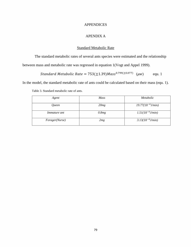
79
APPENDICES
APENDIX A
Standard Metabolic Rate
The standard metabolic rates of several ants species were estimated and the relationship
between mass and metabolic rate was regressed in equation 1(Vogt and Appel 1999).
𝑆𝑡𝑎𝑛𝑑𝑎𝑟𝑑 𝑀𝑒𝑡𝑎𝑏𝑜𝑙𝑖𝑐 𝑅𝑎𝑡𝑒 = 753(±1.39)𝑀𝑎𝑠𝑠0.799(±0.077) (𝜇𝑤) equ. 1
In the model, the standard metabolic rate of ants could be calculated based on their mass (equ. 1).
Table 3. Standard metabolic rate of ants.
Agent Mass Metabolic
Queen 20mg 19.77(10−4J/min)
Immature ant 0.8mg 1.51(10−4J/min)
Forager(Nurse) 2mg 3.13(10−4J/min)

80
APENDIX B
Metabolic Rate for Locomotion
Schilman (Schilman and Roces 2005) measured the net cost of transport (NCOT) for
unladen locomotion in nectar-feeding ant, Camponotus rufipes.
NCOTbody mass=212.3±34.5 (J kg -1m-1)
We assume the NCOT is the universal parameter for calculating the metabolic rate of locomotion
(Mlocomotion) based on mass (equ.2).
𝑀𝑡𝑒𝑙𝑒𝑙𝑒𝑒𝑑𝑒𝑛 = 𝑁𝐶𝑂𝑇𝑏𝑒𝑑𝑦 𝑙𝑒𝑑𝑑 ∙ 𝑚𝑎𝑠𝑠 ∙ 𝑣𝑒𝑙𝑜𝑐𝑖𝑡𝑦 equ. 2
Table 4. Initial metabolic rate of ant worker for locomotion.
𝑁𝐶𝑂𝑇𝑏𝑒𝑑𝑦 𝑙𝑒𝑑𝑑 𝐼𝑛𝑖𝑡𝑖𝑎𝑙 𝑚𝑎𝑠𝑠 𝐼𝑛𝑖𝑡𝑖𝑎𝑙 𝑣𝑒𝑙𝑜𝑐𝑖𝑡𝑦 𝐼𝑛𝑖𝑡𝑖𝑎𝑙 𝑀𝑡𝑒𝑙𝑒𝑙𝑒𝑒𝑑𝑒𝑛
212.3 (J kg -1m-1) 2mg 120cm/min 5.09(10−4J/min)

81
APENDIX C
Metabolic Rate for Growth, Reproduction, and Biosynthesis
Chen (Hou et al. 2008)estimated energy allocation to storage for somatic growth during
ontogeny in equation 3 and energy for biosynthesis in equation 4.
𝑆 = 𝛾 ∙ (𝐵0𝑚3 4⁄ − 𝐵0𝑀−1 4⁄ 𝑚) equ. 3
Here, S is the rate of energy stored for development; 𝛾 is the storage coefficiency; B0 is the
standard metabolic rate; m is the mass at larvae size; M is the mass at adult size. We assume this
equation is valid for ant development (Table 5):
Table 5. Immature ants’ metabolic rate for somatic growth and biosynthesis.
Parameters Estimate References
𝐵0 451.8(10−4J/min) (Vogt 1999)
m 0.8mg (Brian 1973)
M 2mg (Jensen 1978)
𝛾 9 (Hou et al. 2008)
𝑆 3.95(10−4J/min) Equ. 3
In the model, queen is designed to consume energy and store it for laying eggs. We assume the
“immature ant” (0.8mg) develops from vitellogenic follicles (10ug). The energy for development
of per follicle stored by queen could be calculated in equ. 3. In a medium sized colony , about
2,000 vitellogenic follicles were found in ovaries of the queen(Porter 1985). The total energy for
development of follicles stored by queen and energy for queen’s biosynthesis are listed in table 6.

82
Table 6. The rate of energy storage for reproduction.
Parameters Estimate References
𝐵0 451.8(10−4J/min) (Vogt 1999)
m 0.01mg (Meer 1992)
M 0.8mg (Reyes-López 2002)
𝛾 9 (Hou et al. 2008)
𝑛 2000 (Porter 1985)
𝑆per follicle 0.48(10−4J/min) Equ. 3
Stotal follicles 960(10−4J/min) n ∙ Sper follicle
A worker consumes energy to synthesize and accumulate the fat body, which was described in
equation 4(Hou et al. 2008). Here, 𝐵𝑑𝑦𝑛 is energy consumed for biosynthesis; m is the mass of a
worker; M is the mass’ upper threshold of worker.
𝐵𝑑𝑦𝑛 = �𝐵0𝑚3 4⁄ − 𝐵0𝑀−1 4⁄ 𝑚� equ. 4
Table 7. The rate of energy for workers’ biosynthesis.
Parameters Estimate References
𝐵0 451.8(10−4J/min) (Vogt 1999)
m 2mg (Jensen 1978)
M 5mg
𝐵𝑑𝑦𝑛 0.874 (10−4J/min) Equ. 4

83
APENDIX D
Amount of the Food per One Bite
In the infrabuccal pellets of larvae, 1435-1760 food particles were counted, and the
maximum size of food particles swallowed by larvae was 45.8 um, which is approximately
corresponds to the diameter of the esophagus (Glancey 1981). We assume the food particle is a
protein sphere with diameter 45.8 um and density 1.35 g/cm3 (Cummins 1971), and ants have the
same volume of infrabuccal pellets. Every bite, the weight and energy of food in pellets of ants,
could be calculated in equation 5, 6 (Table 8).
𝑊𝑑𝑒𝑒𝑑 = 𝑁𝑑𝑒𝑒𝑑 ∙ �4∙𝜋∙(𝐷 2⁄ )3
3� ∙ 𝐷𝑑𝑒𝑒𝑑 (mg) equ. 5
𝐸𝑑𝑒𝑒𝑑 = 𝑊𝑑𝑒𝑒𝑑 ∙ 𝑐 (10−4J) equ. 6
𝑊𝑑𝑒𝑒𝑑 is the weight of food in one bite; 𝑁𝑑𝑒𝑒𝑑 is the number of food particles in the pellets; 𝐷 is
the diameter of food particle that is approximately corresponds to diameter of the larvae
esophagus; 𝐷𝑑𝑒𝑒𝑑 is the density of food particles; 𝐸𝑑𝑒𝑒𝑑 is the equivalent energy of the food in
one bite; 𝑐 is the weight-energy conversion factor.
Table 8. The amount of food per feeding event.
𝑁𝑑𝑒𝑒𝑑 𝑅(um) 𝐷𝑑𝑒𝑒𝑑
(10−9𝑚𝑔/𝑢𝑚3)
𝑐
(10−4J/mg)
𝑊𝑑𝑒𝑒𝑑
(mg)
𝐸𝑑𝑒𝑒𝑑
(10−4J)
1435 45.8 1.35 190000 0.023 4420

84
APENDIX E
Relationship among Photosynthesis, Temperature, and CO2
The relationships among photosynthesis, temperature and CO2 concentration could be
quantified in equ. 26, 27, 28 (Borjigidai et al. 2006):
𝑃𝑙 = 𝑉𝑐𝑐𝑐𝑐(𝐶𝑖−𝜏∗)𝐶𝑖+𝐾𝑐(1+𝑂 𝐾𝑜� )
− 𝑅𝑑 equ.26
𝑃𝑒 = 𝐽𝑐𝑐𝑐(𝐶𝑖−𝜏∗)4𝐶𝑖+8𝜏∗
− 𝑅𝑑 equ.27
𝑓(𝑇𝑘) = 𝑓(25)𝑒𝑒𝑒 �𝐸𝑐(𝑇𝑘−298)298𝑅𝑇𝑘
� equ.28
Where Vcmax is maximum rate of ribulose-1,5-bisphosphate (RuBP) carboxylation; Jmax is
maximum rate of electron transport; Pc is the photosynthetic rate limited by the RuBP Activity;
Pr is the photosynthetic rate limited by RuBP regeneration; Ci is the concentration of CO2 at
intercellular space, 𝜏∗ is the CO2 compensation point in the absence of day respiration (Rd); Kc
and Ko are Michaelis constants of RuBP carboxylase for CO2 and O2, respectively, and O is the
O2 concentration; f is the value of a parameter; f(25) is f at 25oC; Ea is the activation energy, R is
the gas constant; Tk is leaf temperature in K; The photosynthetic rate is the minimum of Pc and Pr.

85
VITA
XIAOHUI GUO
Education: MS Biology, East Tennessee State University, Johnson City, Tennessee, 2014.
BSc. Biological Sciences, China Agriculture University, China, 2005.
Experience: Teaching Associate, Department of Biological Sciences, East Tennessee State
University, Johnson City, TN 2011-2013.
Awards and Grants: Thesis Scholarship, Graduate of School, East Tennessee State University,
Johnson City, Tennessee 2013.
Conferences: Attended Appalachian Student Research Forum, East Tennessee State
University, Johnson City, TN 2012; Appalachian Student Research Forum,
East Tennessee State University, Johnson City, TN 2013; Appalachian
Student Research Forum, East Tennessee State University, Johnson City, TN
2014.
Technical Skills: SPSS, Netlogo, Anylogic, StarlogoTNG, MEME.