Embed Size (px)
Citation preview
OFR employees Bookstaber and Paddrik contributed to the design of several of the experiments used in this supplement to OFR Working Paper 14-05. The experiments were executed by MITRE staff Bisbee, McMahon, and Slater, and the generation of the output and graphics was executed by MITRE staff Henscheid, under a contract with the OFR. The models in this paper use fictional data.
The Office of Financial Research (OFR) Working Paper Series allows members of the OFR staff and their coauthors to disseminate preliminary research findings in a format intended to generate discussion and critical comments. Papers in the OFR Working Paper Series are works in progress and subject to revision.
Views and opinions expressed are those of the authors and do not necessarily represent official positions or policy of the OFR, Treasury, or MITRE. Comments and suggestions for improvements are welcome and should be directed to the authors. OFR working papers may be quoted without additional permission.
An Agent-based Model for Financial Vulnerability: Supplementary Material Anthony J. Bisbee The MITRE Corporation [email protected]
Rick Bookstaber Office of Financial Research [email protected]
Shaun M. Brady The MITRE Corporation [email protected]
Carl D. Burke The MITRE Corporation [email protected]
Christine E. Harvey The MITRE Corporation [email protected]
Zoe A. Henscheid The MITRE Corporation [email protected]
Matthew T. K. Koehler The MITRE Corporation [email protected]
Matthew T. McMahon The MITRE Corporation [email protected]
Mark Paddrik Office of Financial Research [email protected]
David Slater The MITRE Corporation [email protected]
Brian F. Tivnan The MITRE Corporation [email protected]
14-05-A | March 26, 2015
OFFICE OF FINANCIAL RESEARCH 2
Experimenting with the Model
Introduction The 3-2-2-1 Model tested here is the model presented in An Agent-based Model for Financial Vulnerability applied to three assets, two hedge funds, two trading units, and one cash provider. This document provides details on the no shock and price shock experiments that were conducted for the 3-2-2-1 Model.
This document contains the following main sections:
1. The 3-2-2-1 Model Parameters. This section provides a listing of the parameters, as well as their default values, reasonable range of values, and definition.
2. The Benchmark Experiment: No Shock and 10% Shock. This section provides an analysis of the results of the experiment that was conducted using the benchmark/default values for the 3-2-2-1 Model.
3. Excursions to the Benchmark Experiment: 15% Price Shock and 20% Price Shock. This section contains an analysis of the results of the Excursions to the Benchmark Experiment.
4. The Broad Price Shock Experiment for the 3-2-2-1 Model. This section describes the Broad Price Shock Experiment and its results.
3-2-2-1 Model Parameters Table 1 provides a listing of the 3-2-2-1 Model parameters that are related to the assets. Each of the assets has its own parameters, and this table provides a summary of those parameters.
Parameters For the Assets
Parameter Name Default Value
Reasonable Range of Values Definition
initialPricei 100 Initial Price of Asset i epsilon_Pt_sigmai 0.01 0.01 to 0.02 Standard deviation for day-to-day
change in Asset i’s price. The daily change in asset price is modeled as a normally distributed random variable with mean of zero.
%DropPerBi 1 0.5 to 2 Affects Asset i’s liquidity and is the percentage drop per billion dollars
Table 1: Parameters for the Assets in the 3-2-2-1 Model
Table 2 provides a listing of the 3-2-2-1 Model parameters that are related to the cash provider.
Parameters For the Model’s Cash Provider

OFFICE OF FINANCIAL RESEARCH 3
Parameter Name Default Value
Reasonable Range of Values Definition
CP_Haircut_Bi 0.15 0.1 to 0.2 Cash Provider’s Haircut for Bank Dealer i. This value may be different for each Bank Dealer.
Reset_Switch_CP TRUE TRUE and FALSE Will the Cash Provider’s haircuts to both bank dealers be set equal to each other?
Reset_CP_Haircut 0.15 0.1 to 0.2 Value for both of the Bank Dealers’ haircuts received from the Cash Provider.
enforceHaircutLeverageRelationship? TRUE TRUE and FALSE Setting this parameter to true will overwrite maxLeverage values for the Hedge Funds and Trading Units
Table 2: Parameters for the Cash Provider in the 3-2-2-1 Model
Table 3 provides a listing of the 3-2-2-1 Model parameters that are related to the Hedge Funds. Each of the hedge funds has its own parameters, and this table provides a summary of those parameters.
Parameters For the Model’s Hedge Funds
Parameter Name Default Value
Reasonable Range of Values Definition
initialCapital_HFi 10000000000 Initial amount of capital that Hedge Fund i has.
LBuffer%_HFi 90 0.90 to 0.95 For Hedge Fund i, the percent of max leverage that the trading unit will try not to exceed.
LTarget%_HFi 85 0.80 to 0.90 Hedge Fund i’s Leverage Target which is some percentage of Hedge Fund i’s leverage buffer.
Asset0HFi 0.5 0.0 to 1.0 Hedge Fund i’s allocation in Asset 0.
Asset1HFi 0.5 0.0 to 1.0 Hedge Fund i’s allocation in Asset 1.
Asset2HFi 0 0.0 to 1.0 Hedge Fund i’s allocation in Asset 2.
Table 3: Parameters for the Hedge Funds in the 3-2-2-1 Model
OFFICE OF FINANCIAL RESEARCH 4
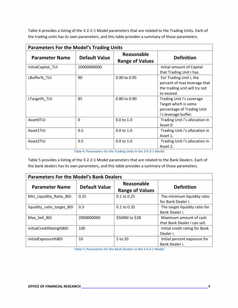
Table 4 provides a listing of the 3-2-2-1 Model parameters that are related to the Trading Units. Each of the trading units has its own parameters, and this table provides a summary of those parameters.
Parameters For the Model’s Trading Units
Parameter Name Default Value Reasonable Range of Values Definition
initialCapital_TUi 10000000000 Initial amount of Capital that Trading Unit i has.
LBuffer%_TUi 90 0.90 to 0.95 For Trading Unit i, the percent of max leverage that the trading unit will try not to exceed.
LTarget%_TUi 85 0.80 to 0.90 Trading Unit i’s Leverage Target which is some percentage of Trading Unit i’s leverage buffer.
Asset0TUi 0 0.0 to 1.0 Trading Unit i’s allocation in Asset 0.
Asset1TUi 0.5 0.0 to 1.0 Trading Unit i’s allocation in Asset 1.
Asset2TUi 0.5 0.0 to 1.0 Trading Unit i’s allocation in Asset 2.
Table 4: Parameters for the Trading Units in the 3-2-2-1 Model
Table 5 provides a listing of the 3-2-2-1 Model parameters that are related to the Bank Dealers. Each of the bank dealers has its own parameters, and this table provides a summary of those parameters.
Parameters For the Model’s Bank Dealers
Parameter Name Default Value Reasonable Range of Values Definition
Min_Liquidity_Ratio_BDi 0.25 0.1 to 0.25 The minimum liquidity ratio for Bank Dealer i.
liquidity_ratio_target_BDi 0.3 0.1 to 0.35 The target liquidity ratio for Bank Dealer i.
Max_Sell_BDi 2000000000 $500M to $2B Maximum amount of cash that Bank Dealer i can sell.
initialCreditRating%BDi 100 Initial credit rating for Bank Dealer i.
initialExposure%BDi 10 5 to 20 Initial percent exposure for Bank Dealer i.
Table 5: Parameters for the Bank Dealers in the 3-2-2-1 Model
OFFICE OF FINANCIAL RESEARCH 5
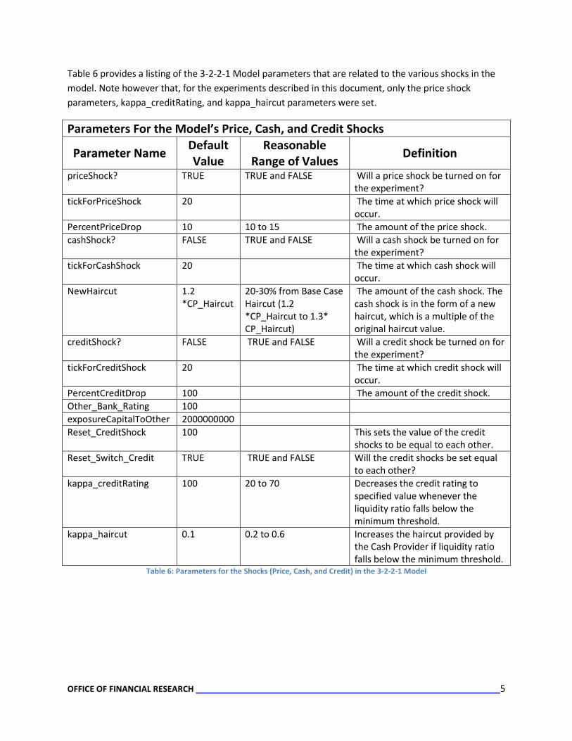
Table 6 provides a listing of the 3-2-2-1 Model parameters that are related to the various shocks in the model. Note however that, for the experiments described in this document, only the price shock parameters, kappa_creditRating, and kappa_haircut parameters were set.
Parameters For the Model’s Price, Cash, and Credit Shocks
Parameter Name Default Value
Reasonable Range of Values Definition
priceShock? TRUE TRUE and FALSE Will a price shock be turned on for the experiment?
tickForPriceShock 20 The time at which price shock will occur.
PercentPriceDrop 10 10 to 15 The amount of the price shock. cashShock? FALSE TRUE and FALSE Will a cash shock be turned on for
the experiment? tickForCashShock 20 The time at which cash shock will
occur. NewHaircut 1.2
*CP_Haircut 20-30% from Base Case Haircut (1.2 *CP_Haircut to 1.3* CP_Haircut)
The amount of the cash shock. The cash shock is in the form of a new haircut, which is a multiple of the original haircut value.
creditShock? FALSE TRUE and FALSE Will a credit shock be turned on for the experiment?
tickForCreditShock 20 The time at which credit shock will occur.
PercentCreditDrop 100 The amount of the credit shock. Other_Bank_Rating 100 exposureCapitalToOther 2000000000 Reset_CreditShock 100 This sets the value of the credit
shocks to be equal to each other. Reset_Switch_Credit TRUE TRUE and FALSE Will the credit shocks be set equal
to each other? kappa_creditRating 100 20 to 70 Decreases the credit rating to
specified value whenever the liquidity ratio falls below the minimum threshold.
kappa_haircut 0.1 0.2 to 0.6 Increases the haircut provided by the Cash Provider if liquidity ratio falls below the minimum threshold.
Table 6: Parameters for the Shocks (Price, Cash, and Credit) in the 3-2-2-1 Model

OFFICE OF FINANCIAL RESEARCH 6
The Benchmark Experiment: No Shock and 10% Shock
Key Parameter Values for 3-2-2-1 Benchmark Runs
Table 7 describes the various levels for each of the key parameters for the 3-2-2-1 Benchmark experiment.
Parameter Name Value Capital for HF1, HF2, TU1, and TU2 $10 B Epsilon_Pt_sigma for Asset 0, Asset 1, and Asset 2 0.01 %PercentDropPerB for Asset 0, Asset 1, and Asset 2 1.0 Initial Asset Price for Asset 0, Asset 1, and Asset 2 $100 Leverage Target Ratio for HF1, HF2, TU1, and TU2 85 of Leverage Buffer Leverage Buffer Ratio for HF1, HF2, TU1, and TU2 0.9 of Max Leverage Asset Allocation for HF1 0.50 in Asset 0 and 0.50 in Asset 1 Asset Allocation for HF2, TU1, and TU2 0.50 in Asset 1 and 0.50 in Asset 2 CP Haircut for BD1 and BD2 0.15 Other Bank Rating 100 Exposure Capital To Other $2B kappa Credit Rating 100 kappa Haircut 0.1 Min Liquidity Ratio for BD1 0.25 Min Liquidity Ratio for BD2 0.2 Liquidity Ratio Target for BD1 and BD2 0.3 Max Sell for BD1 and BD2 $2B Initial Credit Rating Percentage for BD1 and BD2 100 Initial Exposure Percentage for BD1 and BD2 10 Run Duration 60 Time of Price Shock (if applicable) 20 Percent Price Drop (if applicable) 10
Table 7: Parameter Settings for the Benchmark DOE conducted for the 3-2-2-1 Model
The No Shock and 10% Price Shock Benchmark Design Points for the Benchmark Experiment were each run for 1000 different random seeds – so each had 1000 replicates.

OFFICE OF FINANCIAL RESEARCH 7
Benchmark 3-2-2-1 Results
No Shock Experimental Design Results
There were no Hedge Fund qDemand events in 1000 realizations of the No Shock Benchmark Design Point. This means that the 3-2-2-1 Benchmark values provide a good starting point for stress testing, since no qDemand events were seen in the unshocked scenario.
Figure 1 depicts the price time series for all three assets for the No Shock Benchmark experimental design point.
Figure1: Time series for the three assets in the 3-2-2-1 Model Benchmark No Shock Design Point runs.
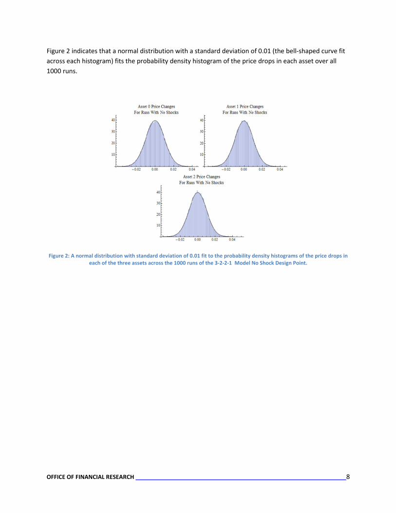
Since there is no shock to the system, the changes in price (relative to the initial asset price of 100) should be normally distributed with a standard deviation of 0.01. This is due to the fact that each asset has a change in price at each time step equivalent to a random draw from a N(0,1) with epsilon_Pt_sigma = 0.01.
OFFICE OF FINANCIAL RESEARCH 8
Figure 2 indicates that a normal distribution with a standard deviation of 0.01 (the bell-shaped curve fit across each histogram) fits the probability density histogram of the price drops in each asset over all 1000 runs.
Figure 2: A normal distribution with standard deviation of 0.01 fit to the probability density histograms of the price drops in each of the three assets across the 1000 runs of the 3-2-2-1 Model No Shock Design Point.

OFFICE OF FINANCIAL RESEARCH 9
Benchmark 10% Price Shock Experimental Design Results
Number of qDemand Events for the Hedge Funds and the Trading Units The first metrics examined for the 10% Price Shock Design Point of the Benchmark Experiment were: the number of occurrences of (1) Hedge Fund qDemand events and (2) Trading Unit qDemand events exhibited in each run. The histogram on the left in Figure 3 below displays the total number of Hedge Fund qDemand events per run; the histogram on the right displays the total number of Trading Unit qDemand events per run. Beneath each histogram is the associated tabular data.
Figure 3: Histogram of the total number of Hedge Fund and Trading qDemand events per run in the 3-2-2-1 Model Benchmark 10% Price Shock Design Point.
For most runs in the Benchmark 10% Price Shock Design Point, when Hedge Fund qDemand events occur, there are between 2 and 14 Hedge Fund qDemand events. Note that in 742 out of 1000 runs, no hedge fund qDemand events occurred. There are fewer Trading Unit qDemand events than Hedge Fund qDemand events occurring in the Benchmark 10% Price Shock Design Point. In 981 of the 1000 runs, no Trading Unit qDemand events occurred.
Number of qDemand Events for each Hedge Fund and Trading Unit In addition to looking at the total number of qDemand events that occur across all of the hedge funds and trading units, we can also look at the number of qDemand events at each hedge fund and trading unit. Figure 4 depicts the results for the NetLogo 3-2-2-1 Benchmark 10% Price Shock design Point .

OFFICE OF FINANCIAL RESEARCH 10
Figure 4: Histogram of the total number of qDemand events (for each hedge fund and trading unit) per run in the 3-2-2-1 Model Benchmark 10% Price Shock Design Point.
One can see that, in general, Hedge Fund 1 is the only entity to have qDemand events when Asset 0 receives a 10% price shock. It should be noted that Hedge Fund 1 is the only entity that has an allocation in the shocked asset (Asset 0).
OFFICE OF FINANCIAL RESEARCH 11
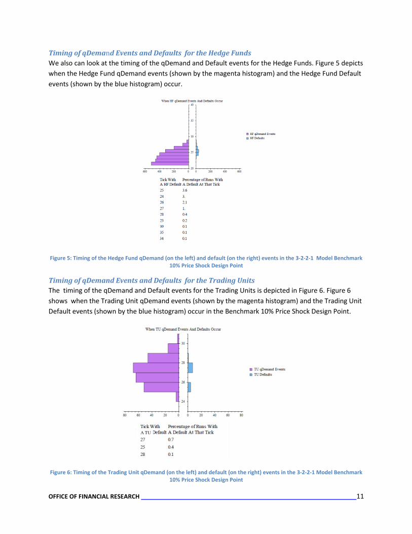
Timing of qDemand Events and Defaults for the Hedge Funds We also can look at the timing of the qDemand and Default events for the Hedge Funds. Figure 5 depicts when the Hedge Fund qDemand events (shown by the magenta histogram) and the Hedge Fund Default events (shown by the blue histogram) occur.
Figure 5: Timing of the Hedge Fund qDemand (on the left) and default (on the right) events in the 3-2-2-1 Model Benchmark 10% Price Shock Design Point
Timing of qDemand Events and Defaults for the Trading Units The timing of the qDemand and Default events for the Trading Units is depicted in Figure 6. Figure 6 shows when the Trading Unit qDemand events (shown by the magenta histogram) and the Trading Unit Default events (shown by the blue histogram) occur in the Benchmark 10% Price Shock Design Point.
Figure 6: Timing of the Trading Unit qDemand (on the left) and default (on the right) events in the 3-2-2-1 Model Benchmark 10% Price Shock Design Point

OFFICE OF FINANCIAL RESEARCH 12
Sequencing of qDemand Events and Defaults
In addition to looking at the timing of the Hedge Fund and Trading Unit qDemand events and defaults, we also looked at the sequencing of those events. There are a total of thirteen events of interest:
1) Price Shock 2) qDemand Event for Hedge Fund 1 Asset 0 3) qDemand Event for Hedge Fund 1 Asset 1 4) qDemand Event for Hedge Fund 2 Asset 1 5) qDemand Event for Hedge Fund 2 Asset 2 6) Default of Hedge Fund 1 7) Default of Hedge Fund 2 8) qDemand Event for Trading Unit 1 Asset 1 9) qDemand Event for Trading Unit 1 Asset 2 10) qDemand Event for Trading Unit 2 Asset 1 11) qDemand Event for Trading Unit 2 Asset 2 12) Default of Trading Unit 1 13) Default of Trading Unit 2
Figure 7 depicts the event sequencing for the Benchmark 10% Price Shock Design Point. This figure indicates that there are 742 out of 1000 runs where there were no qDemand events after the price shock event. This figure also shows that there never is a Hedge Fund default without a qDemand event preceding it. Further very rarely (27 of the 1000 replicates) is there any “contagion” – where qDemand events were seen in the hedge fund and trading units that had no allocation in the shocked asset. And, only 4 of these 27 realizations resulted in both hedge funds and both trading units defaulting.

OFFICE OF FINANCIAL RESEARCH 13
Figure 7: Event Sequence Diagram for the Hedge Fund and Trading Unit Events of Interest in the 3-2-2-1 Model Benchmark 10% Price Shock Design Point.

OFFICE OF FINANCIAL RESEARCH 14
Probability of qDemand Events and Defaults at Each Time Step Instead of working in “event time”, we can also look at the events in chronological time. Figure 8 depicts the probability of each of the thirteen events of interest occurring for time steps 15-40 of the 3-2-2-1 Benchmark 10% Price Shock Design Point.
Figure 8: Probability of the Hedge Fund and Trading Unit Events of Interest Occurring in Time Steps 15-40 of the 3-2-2-1 Model Benchmark 10% Price Shock Design Point.
Figure 9 depicts the same information as Figure 8. However, it does so by depicting the log10 of the probability to allow one to see more gradation and discern between small probabilities and zero probabilities.
Figure 9: Log10 of the Probability of the Hedge Fund and Trading Unit Events of Interest Occurring in Time Steps 15-40 of the 3-2-2-1 Model Benchmark 10% Price Shock Design Point.
OFFICE OF FINANCIAL RESEARCH 15
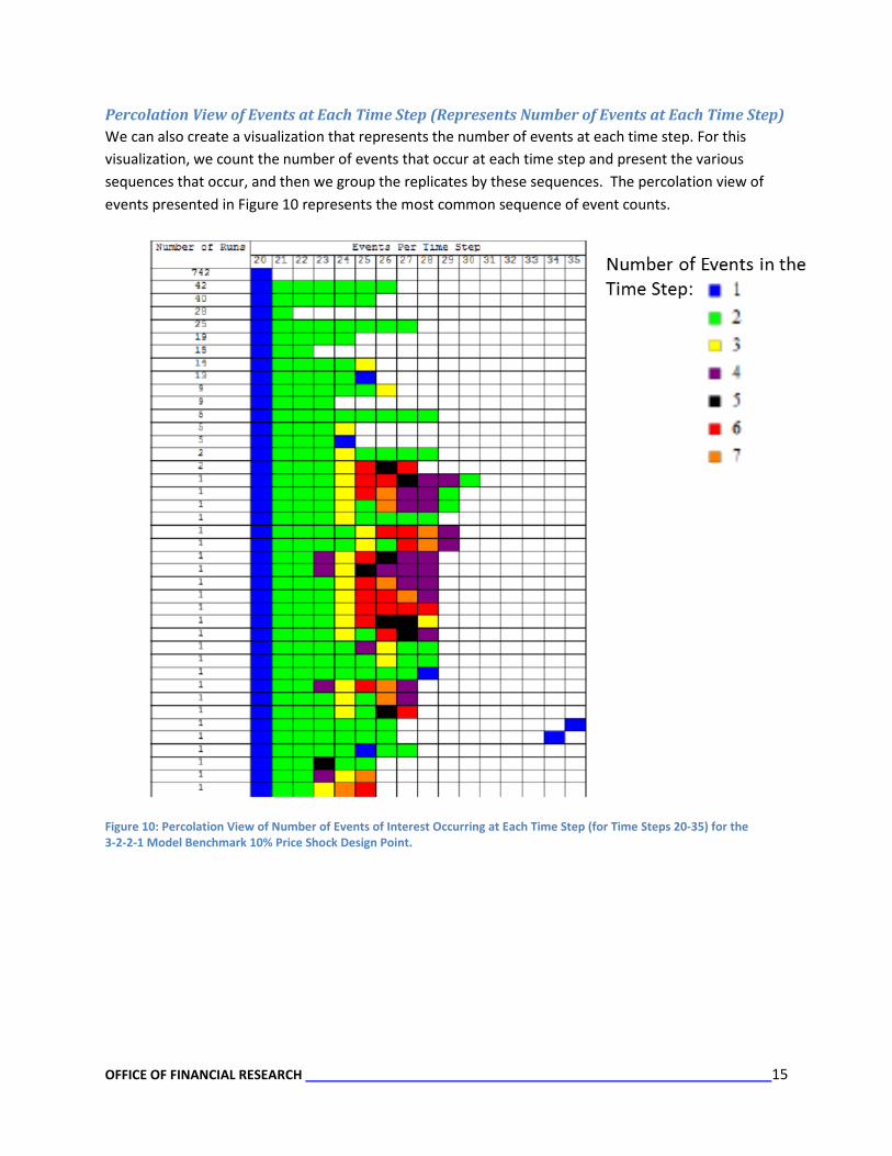
Percolation View of Events at Each Time Step (Represents Number of Events at Each Time Step) We can also create a visualization that represents the number of events at each time step. For this visualization, we count the number of events that occur at each time step and present the various sequences that occur, and then we group the replicates by these sequences. The percolation view of events presented in Figure 10 represents the most common sequence of event counts.
Figure 10: Percolation View of Number of Events of Interest Occurring at Each Time Step (for Time Steps 20-35) for the 3-2-2-1 Model Benchmark 10% Price Shock Design Point.

OFFICE OF FINANCIAL RESEARCH 16
Excursions to the Benchmark Experiment: 15% Price Shock and 20% Price Shock Since the Benchmark Price Shock of 10% was not expected to have significant impacts on the hedge funds and trading units, price shock excursions were conducted. For these excursions, all of the benchmark values were used for the key parameters, except the price shock was set to either 15% or 20%. Table 8 describes the two price shock excursions that were conducted. These excursions also were run for 1000 different seeds – i.e., each had 1000 replicates.
Excursion Parameter Name Value
Excursion 1 Percent Price Drop 15 All Other Parameters As Specified in Table 7
Excursion 2 Percent Price Drop 20 All Other Parameters As Specified in Table 7
Table 8: Parameters Varied for the Price Shock Excursions conducted for the 3-2-2-1 Model
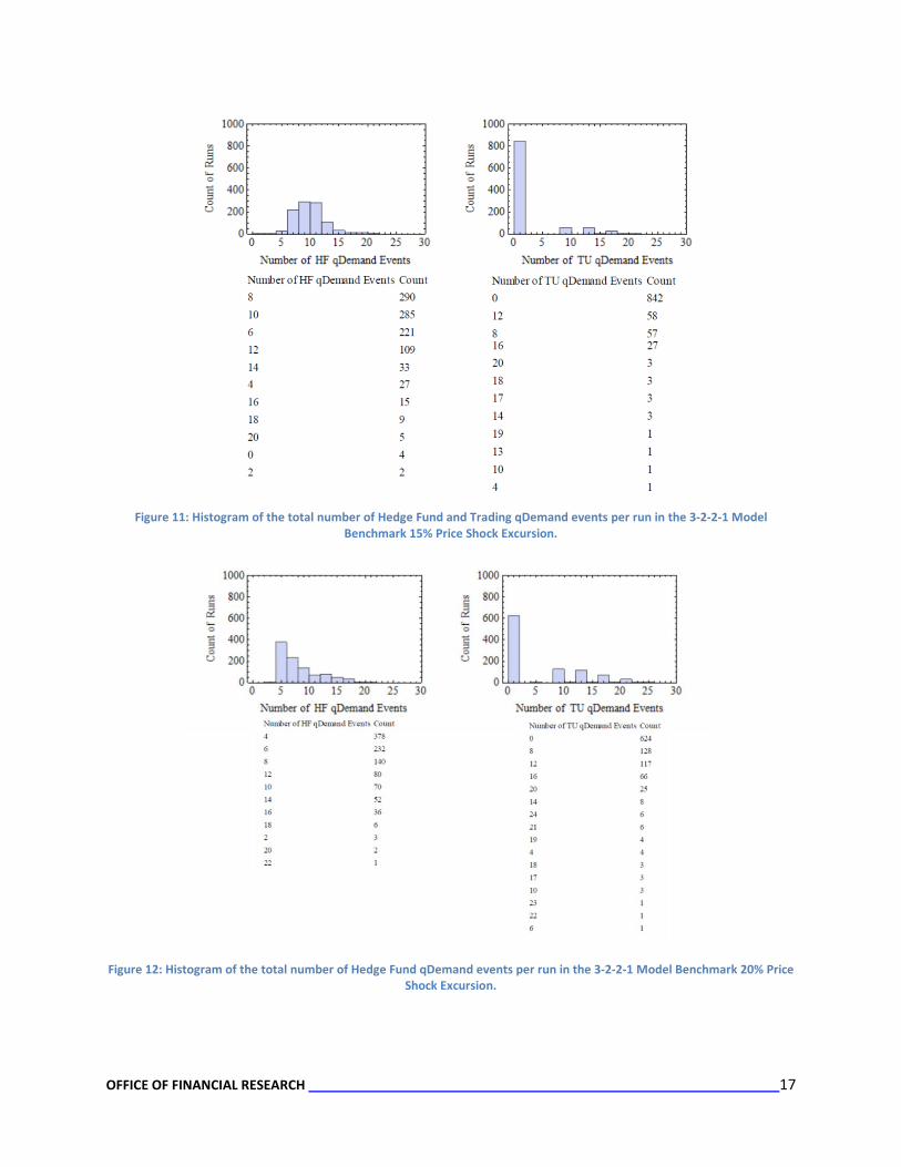
Number of qDemand Events for the Hedge Funds and the Trading Units The first metrics examined are the number of occurrences of Hedge Fund qDemand events and Trading Unit qDemand events each run has. Figure 11 depicts these metrics for the Benchmark 15% Price Shock Excursion and Figure 12 depicts these for the Benchmark 20% Price Shock Excursion. In these figures, the histogram on the left displays the total number of Hedge Fund qDemand events per run; the histogram on the right displays the total number of Trading Unit qDemand events per run. Beneath each histogram is the associated tabular data.
Unlike the Benchmark 10% Price Shock Design Point, for the Benchmark 15% Price Shock Excursion, there was always a Hedge Fund qDemand event; and for the majority of the runs, there are between 6 and 14 Hedge Fund qDemand events. Similar to the Benchmark 10% Price Shock Design Point, there are many less Trading Unit qDemand events than there are Hedge Fund qDemand events occurring in the Benchmark 15% Price Shock Excursion. In 842 of the 1000 runs, no Trading Unit qDemand events occurred.
Similarly for the Prototype Benchmark 20% Price Shock Excursion, there was always a HF qDemand event; and for the majority of the runs, there are between 4 and 16 Hedge Fund qDemand events. Similar to the Prototype Benchmark 10% Price Shock Design Point, there are many less Trading Unit qDemand events occurring in the NetLogo Benchmark 20% Price Shock Excursion. In 624 of the 1000 runs, no Trading Unit qDemand events occurred.
OFFICE OF FINANCIAL RESEARCH 17
Figure 11: Histogram of the total number of Hedge Fund and Trading qDemand events per run in the 3-2-2-1 Model Benchmark 15% Price Shock Excursion.
Figure 12: Histogram of the total number of Hedge Fund qDemand events per run in the 3-2-2-1 Model Benchmark 20% Price Shock Excursion.

OFFICE OF FINANCIAL RESEARCH 18
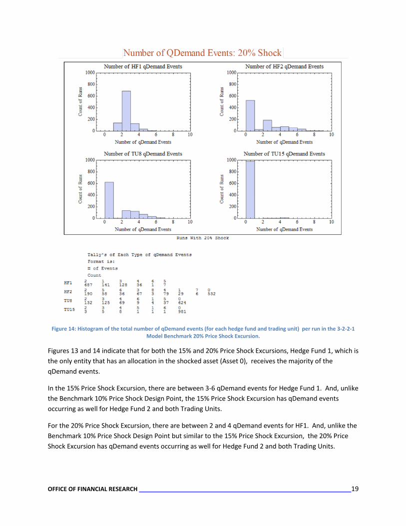
Number of qDemand Events for each Hedge Fund and Trading Unit In addition to looking at the total number of qDemand events that occur across all of the hedge funds and trading units, we can also look at the number of qDemand events at each hedge fund and trading unit. Figure 13 depicts the results for the Benchmark 15% Price Shock Excursion and Figure 14 depicts the results for the Benchmark 20% Price Shock Excursion.
Figure 13: Histogram of the total number of qDemand events (for each hedge fund and trading unit) per run in the 3-2-2-1 Model Benchmark 15% Price Shock Excursion.
OFFICE OF FINANCIAL RESEARCH 19
Figure 14: Histogram of the total number of qDemand events (for each hedge fund and trading unit) per run in the 3-2-2-1 Model Benchmark 20% Price Shock Excursion.
Figures 13 and 14 indicate that for both the 15% and 20% Price Shock Excursions, Hedge Fund 1, which is the only entity that has an allocation in the shocked asset (Asset 0), receives the majority of the qDemand events.
In the 15% Price Shock Excursion, there are between 3-6 qDemand events for Hedge Fund 1. And, unlike the Benchmark 10% Price Shock Design Point, the 15% Price Shock Excursion has qDemand events occurring as well for Hedge Fund 2 and both Trading Units.
For the 20% Price Shock Excursion, there are between 2 and 4 qDemand events for HF1. And, unlike the Benchmark 10% Price Shock Design Point but similar to the 15% Price Shock Excursion, the 20% Price Shock Excursion has qDemand events occurring as well for Hedge Fund 2 and both Trading Units.
OFFICE OF FINANCIAL RESEARCH 20
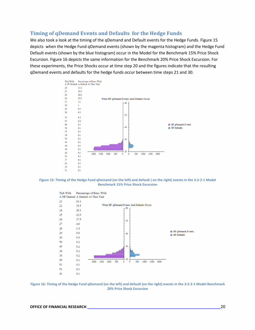
Timing of qDemand Events and Defaults for the Hedge Funds We also took a look at the timing of the qDemand and Default events for the Hedge Funds. Figure 15 depicts when the Hedge Fund qDemand events (shown by the magenta histogram) and the Hedge Fund Default events (shown by the blue histogram) occur in the Model for the Benchmark 15% Price Shock Excursion. Figure 16 depicts the same information for the Benchmark 20% Price Shock Excursion. For these experiments, the Price Shocks occur at time step 20 and the figures indicate that the resulting qDemand events and defaults for the hedge funds occur between time steps 21 and 30.
Figure 15: Timing of the Hedge Fund qDemand (on the left) and default ( on the right) events in the 3-2-2-1 Model Benchmark 15% Price Shock Excursion
Figure 16: Timing of the Hedge Fund qDemand (on the left) and default (on the right) events in the 3-2-2-1 Model Benchmark 20% Price Shock Excursion

OFFICE OF FINANCIAL RESEARCH 21
Timing of qDemand Events and Defaults for the Trading Units We also took a look at the timing of the qDemand and Default events for the Trading Units. Figure 17 depicts when the Trading Unit qDemand events (shown by the magenta histogram) and the Trading Unit Default events (shown by the blue histogram) occur in the 3-2-2-1 Model for the Benchmark 15% Price Shock Excursion. Figure 18 depicts the same information for the Benchmark 20% Price Shock Excursion. For these experiments, the Price Shocks occur at time step 20 and the figures below indicate that the resulting qDemand events for the trading units occur between time steps 23 and 30; and the resulting defaults occur between time steps 25 and 28.
Figure 17: Timing of the Trading Unit qDemand (on the left) and default (on the right) events in the 3-2-2-1 Model Benchmark 15% Price Shock Excursion
Figure 18: Timing of the Trading Unit qDemand (on the left) and default (on the right) events in the 3-2-2-1 Model Benchmark 20% Price Shock Excursion

OFFICE OF FINANCIAL RESEARCH 22
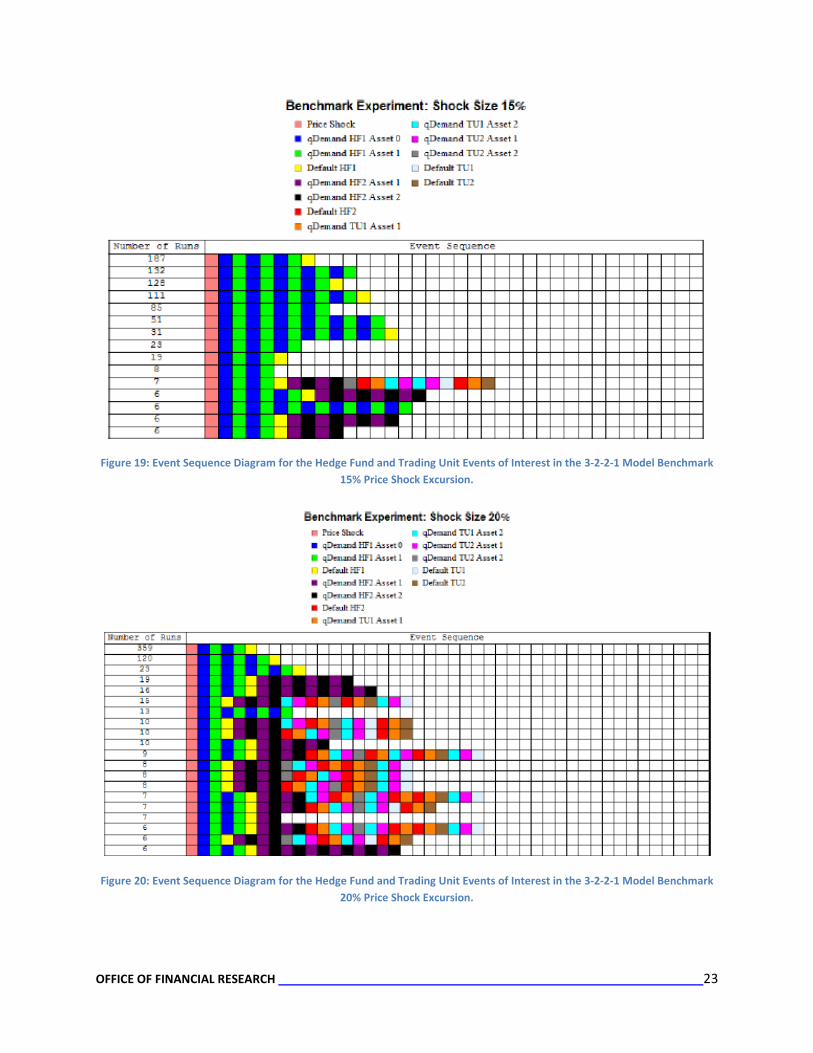
Sequencing of qDemand Events and Defaults In addition to looking at the timing of the Hedge Fund and Trading Unit qDemand events and defaults, we also looked at the sequencing of those events. There are a total of thirteen events of interest:
1) Price Shock 2) qDemand Event for Hedge Fund 1 Asset 0 3) qDemand Event for Hedge Fund 1 Asset 1 4) qDemand Event for Hedge Fund 2 Asset 1 5) qDemand Event for Hedge Fund 2 Asset 2 6) Default of Hedge Fund 1 7) Default of Hedge Fund 2 8) qDemand Event for Trading Unit 1 Asset 1 9) qDemand Event for Trading Unit 1 Asset 2 10) qDemand Event for Trading Unit 2 Asset 1 11) qDemand Event for Trading Unit 2 Asset 2 12) Default of Trading Unit 1 13) Default of Trading Unit 2
Figures 19 and 20 depict the event sequencing for the Benchmark 15% Price Shock Excursion and Benchmark 20% Price Shock Excursion, respectively. Note that these figures only depict the event sequences that resulted in a count of 6 replicates or more.
As one can see in these figures, there never is a Hedge Fund default without a qDemand event preceding it. As expected, the 20% Price Shock results have more qDemand events and defaults in the entities that do not hold the shocked asset (i.e., asset 0) – i.e., Hedge Fund 2 and the two Trading Units.
While the figures only depict the event sequences that resulted in a count of 6 replicates or more, in analyzing all of the event sequences for both the 15% and the 20% Price Shock Excursions we have found the following:
• For the Benchmark Excursion with a 15% Price Shock: There were 4 realizations out of 1000 where the price shock had no effect. There were 250 realizations where Hedge Fund 1 experienced qDemand events that did not result in a default. There were 479 realizations where Hedge Fund 1 experienced a default but neither the second hedge fund nor the trading units had any qDemand events. And 60 realizations where all four entities experienced defaults.
• For the Benchmark Excursion with a 20% Price Shock: There was never an occurrence of a price shock without at least a Hedge Fund 1 qDemand event. There were only 24 realizations where Hedge Fund 1 experienced qDemand events but no defaults. There were 512 realizations where Hedge Fund 1 experienced a default but neither the second hedge fund nor the trading units had any qDemand events. And 166 realizations where all four entities experienced defaults.
OFFICE OF FINANCIAL RESEARCH 23
Figure 19: Event Sequence Diagram for the Hedge Fund and Trading Unit Events of Interest in the 3-2-2-1 Model Benchmark 15% Price Shock Excursion.
Figure 20: Event Sequence Diagram for the Hedge Fund and Trading Unit Events of Interest in the 3-2-2-1 Model Benchmark 20% Price Shock Excursion.
OFFICE OF FINANCIAL RESEARCH 24
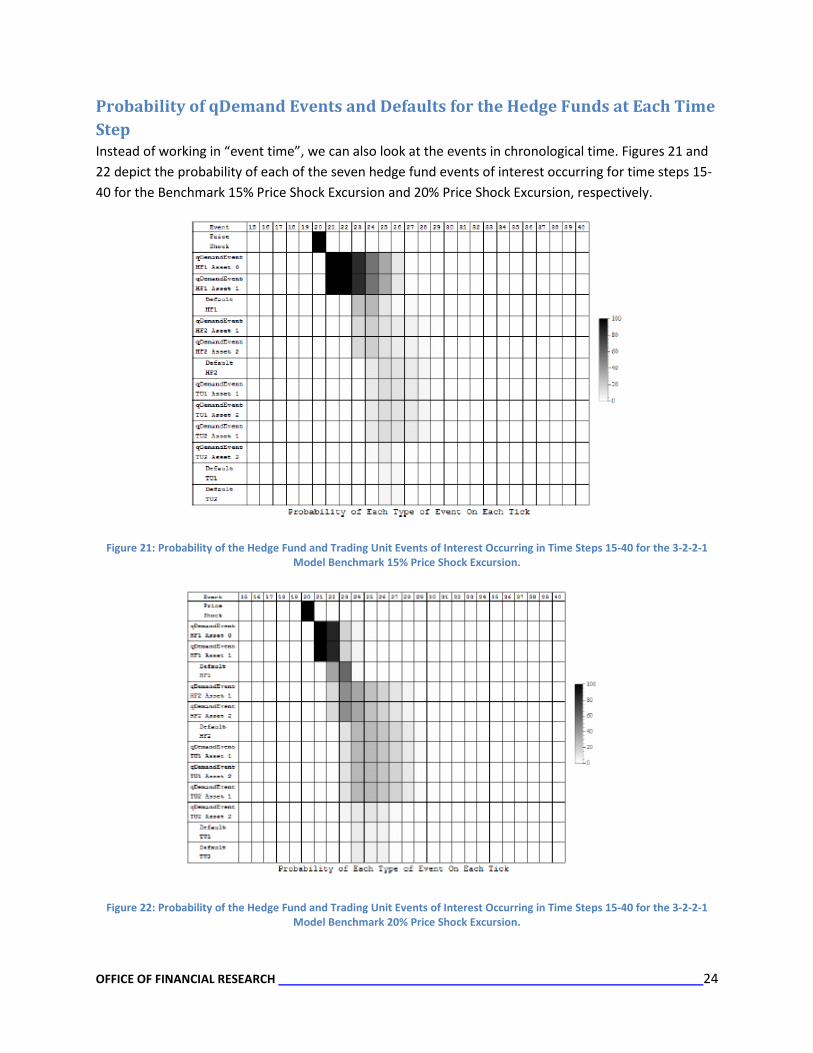
Probability of qDemand Events and Defaults for the Hedge Funds at Each Time Step Instead of working in “event time”, we can also look at the events in chronological time. Figures 21 and 22 depict the probability of each of the seven hedge fund events of interest occurring for time steps 15-40 for the Benchmark 15% Price Shock Excursion and 20% Price Shock Excursion, respectively.
Figure 21: Probability of the Hedge Fund and Trading Unit Events of Interest Occurring in Time Steps 15-40 for the 3-2-2-1 Model Benchmark 15% Price Shock Excursion.
Figure 22: Probability of the Hedge Fund and Trading Unit Events of Interest Occurring in Time Steps 15-40 for the 3-2-2-1 Model Benchmark 20% Price Shock Excursion.

OFFICE OF FINANCIAL RESEARCH 25
Figures 23 and 24 depict the same information as Figures 21 and 22, respectively. However, they do so by depicting the log10 of the probability to allow one to see more gradation and discern between small probabilities and zero probabilities. These figures provide a much better view of the probabilities than were depicted in Figures 21 and 22.
Figure 23: Log10 of the Probability of the Hedge Fund and Trading Unit Events of Interest Occurring in Time Steps 15-40 for the 3-2-2-1 Model Benchmark 15% Price Shock Excursion.
Figure 24: Log10 of the Probability of the Hedge Fund and Trading Unit Events of Interest Occurring in Time Steps 15-40 for the 3-2-2-1 Model Benchmark 20% Price Shock Excursion.
OFFICE OF FINANCIAL RESEARCH 26
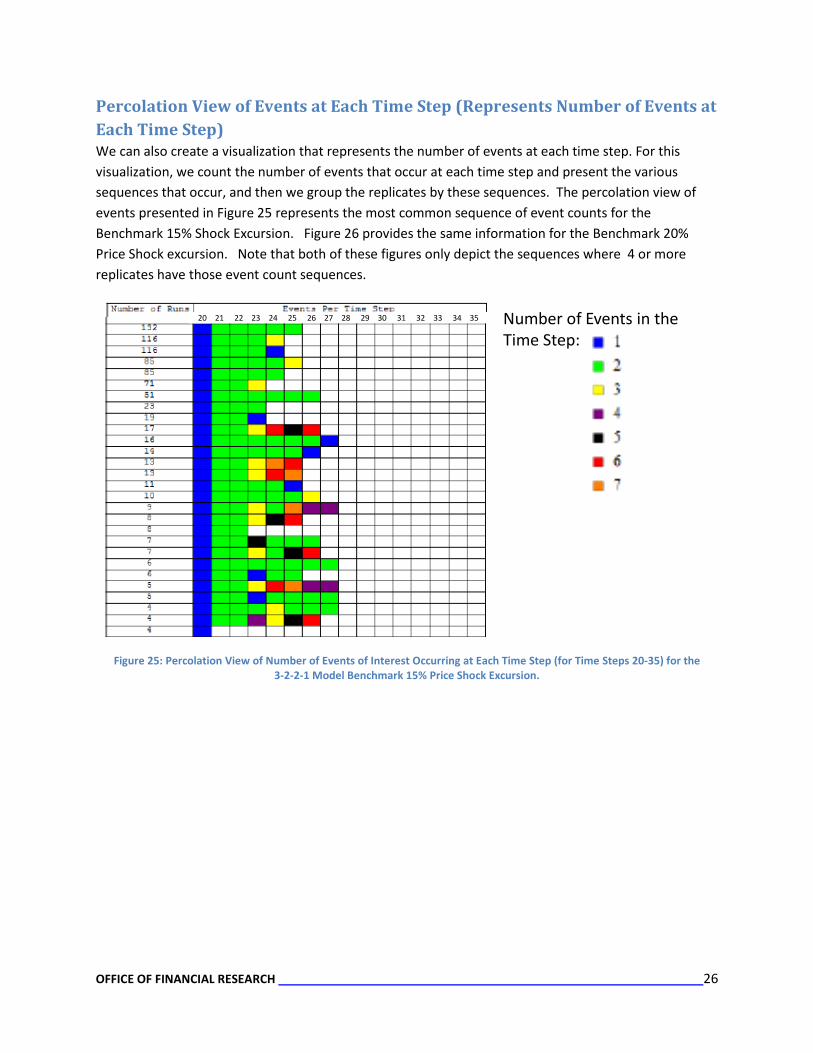
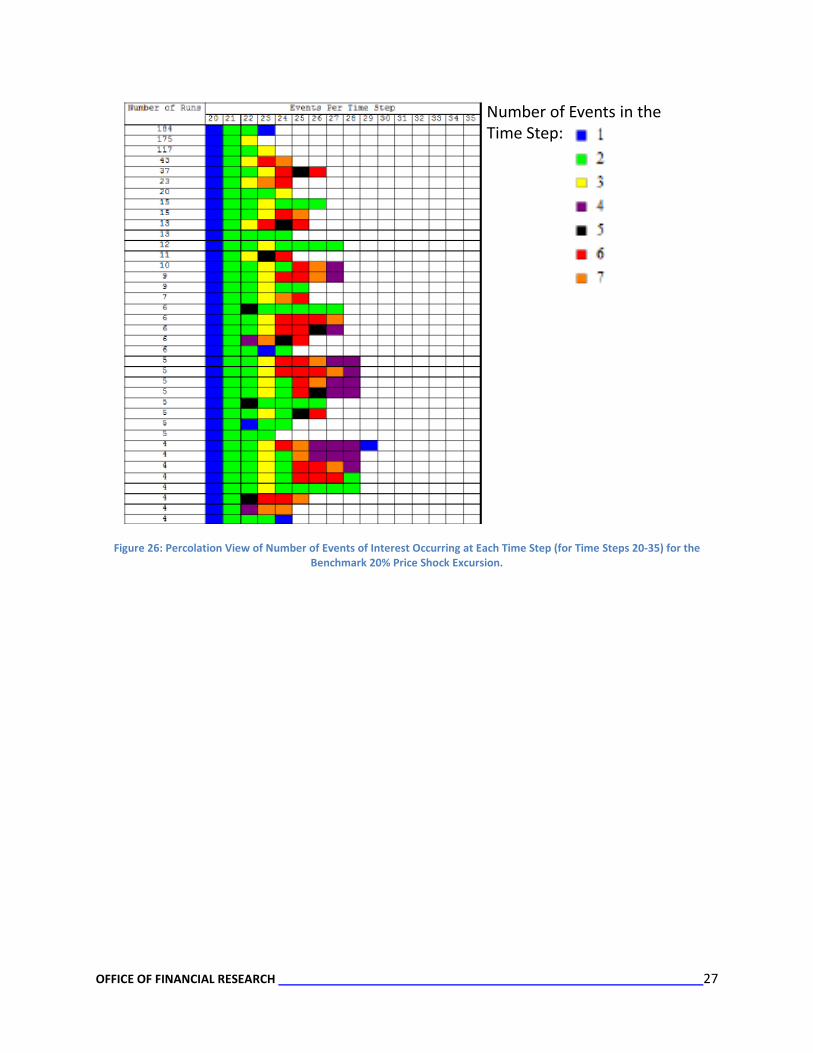
Percolation View of Events at Each Time Step (Represents Number of Events at Each Time Step) We can also create a visualization that represents the number of events at each time step. For this visualization, we count the number of events that occur at each time step and present the various sequences that occur, and then we group the replicates by these sequences. The percolation view of events presented in Figure 25 represents the most common sequence of event counts for the Benchmark 15% Shock Excursion. Figure 26 provides the same information for the Benchmark 20% Price Shock excursion. Note that both of these figures only depict the sequences where 4 or more replicates have those event count sequences.
20 21 22 23 24 25 26 27 28 29 30 31 32 33 34 35 Number of Events in the Time Step:
Figure 25: Percolation View of Number of Events of Interest Occurring at Each Time Step (for Time Steps 20-35) for the 3-2-2-1 Model Benchmark 15% Price Shock Excursion.
OFFICE OF FINANCIAL RESEARCH 27
Number of Events in the Time Step:
Figure 26: Percolation View of Number of Events of Interest Occurring at Each Time Step (for Time Steps 20-35) for the Benchmark 20% Price Shock Excursion.

OFFICE OF FINANCIAL RESEARCH 28
The Broad Price Shock Experiment for the 3-2-2-1 Prototype of the Model The Price Shock Design of Experiments conducted for the 3-2-2-1 NetLogo Prototype of the Model tests for price shocks of 10%, 13% and 15% and includes looking at the effects when several other variables are varied as well.
Parameter Values Varied for the 3-2-2-1 Price Shock Experiment Table 9 describes the various levels for each of the key parameters that were varied for the 3-2-2-1 Price Shock Experiment.
Parameter Name Value PercentPriceDrop 10, 13, 15 %PercentDropPerB for Asset 0, Asset 1, and Asset 2 0.5, 1.0. 2.0 CP Haircut for BD1 and BD2 0.1, 0.13, 0.16, 0.19 kappa Credit Rating 100, 200, 300, 400 kappa Haircut 0.1, 0.2, 0.3, 0.4 Initial Exposure Percentage for BD1 and BD2 10, 20, 40, 80 Max Sell for BD1 and BD2 $500M, $1B, $2B {Min Liquidity Ratio for BD1, Min Liquidity Ratio for BD2, Liquidity Ratio Target for BD1, Liquidity Ratio Target for BD2}
Value 1 = {0.2, 0.25, 0.15, 0.25} Value 2 = {0.25, 0.3, 0.2, 0.3} Value 3 = {0.3, 0.35, 0.25, 0.35}
Table 9: Parameter Values Varied for the Broad Price Shock Experiment conducted for the 3-2-2-1 Model
In Table 9:
• The Percent Price Drop indicates the price shock. • The %PercentDropPerB for each of the three assets are set equal to each other such that
%DropPerB0=%DropPerB1=%DropPerB2. Thus even though there are three parameters being varied, there are only three levels being varied.
• The CP Haircut for the two Bank Dealers are set equal to each other such that CP_Haircut_B1=CP_Haircut_B2. This is accomplished by setting the variable Reset_CP_Haircut equal to the desired level. Thus even though there are two parameters being affected, there are only four levels total being varied.
• The initial exposure percentage for both bank dealers are set equal to each other such that initialExposure%BD1= initialExposure%BD2. Thus even though there are two parameters being affected, there are only four levels total being varied.
• Similarly, the Max Sell for both Bank Dealers are set equal to each other such that Max_Sell_BD1= Max_Sell_BD2. Thus even though there are two parameters being varied, there are only three levels total being varied.
• Finally, the following liquidity ratio parameters have their levels varied together in lockstep: Min_Liquidity_Ratio_BD1, Min_Liquidity_Ratio_BD2, liquidity_ratio_target_BD1, and liquidity_ratio_target_BD2. The three different sets of levels for each of these variables are indicated in “{}” in the table above.
OFFICE OF FINANCIAL RESEARCH 29
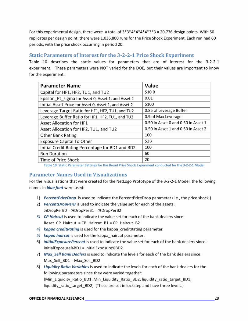
For this experimental design, there were a total of 3*3*4*4*4*4*3*3 = 20,736 design points. With 50 replicates per design point, there were 1,036,800 runs for the Price Shock Experiment. Each run had 60 periods, with the price shock occurring in period 20.
Static Parameters of Interest for the 3-2-2-1 Price Shock Experiment Table 10 describes the static values for parameters that are of interest for the 3-2-2-1 experiment. These parameters were NOT varied for the DOE, but their values are important to know for the experiment.
Parameter Name Value Capital for HF1, HF2, TU1, and TU2 $10 B Epsilon_Pt_sigma for Asset 0, Asset 1, and Asset 2 0.01 Initial Asset Price for Asset 0, Asset 1, and Asset 2 $100 Leverage Target Ratio for HF1, HF2, TU1, and TU2 0.85 of Leverage Buffer Leverage Buffer Ratio for HF1, HF2, TU1, and TU2 0.9 of Max Leverage Asset Allocation for HF1 0.50 in Asset 0 and 0.50 in Asset 1 Asset Allocation for HF2, TU1, and TU2 0.50 in Asset 1 and 0.50 in Asset 2 Other Bank Rating 100 Exposure Capital To Other $2B Initial Credit Rating Percentage for BD1 and BD2 100 Run Duration 60 Time of Price Shock 20
Table 10: Static Parameter Settings for the Broad Price Shock Experiment conducted for the 3-2-2-1 Model
Parameter Names Used in Visualizations For the visualizations that were created for the NetLogo Prototype of the 3-2-2-1 Model, the following names in blue font were used:
1) PercentPriceDrop is used to indicate the PercentPriceDrop parameter (i.e., the price shock.) 2) PercentDropPerB is used to indicate the value set for each of the assets:
%DropPerB0 = %DropPerB1 = %DropPerB2 3) CP Haircut is used to indicate the value set for each of the bank dealers since:
Reset_CP_Haircut = CP_Haircut_B1 = CP_Haircut_B2 4) kappa creditRating is used for the kappa_creditRating parameter. 5) kappa haircut is used for the kappa_haircut parameter. 6) initialExposurePercent is used to indicate the value set for each of the bank dealers since :
initialExposure%BD1 = initialExposure%BD2 7) Max_Sell Bank Dealers is used to indicate the levels for each of the bank dealers since:
Max_Sell_BD1 = Max_Sell_BD2 8) Liquidity Ratio Variables is used to indicate the levels for each of the bank dealers for the
following parameters since they were varied together: {Min_Liquidity_Ratio_BD1, Min_Liquidity_Ratio_BD2, liquidity_ratio_target_BD1, liquidity_ratio_target_BD2} (These are set in lockstep and have three levels.)

OFFICE OF FINANCIAL RESEARCH 30
The next sections describe the type of visualizations/analyses that were conducted for the Broad Price Shock Experiment.
Sequencing of qDemand Events and Defaults In looking at the event sequences for this set of runs, there are a total of nine events of interest:
1) Price Shock 2) qDemand Event for Hedge Fund 1 (Asset 0 and Asset 1)1 3) Default of Hedge Fund 1 4) qDemand Event for Hedge Fund 2 (Asset 1 and Asset2) 5) Default of Hedge Fund 2 6) qDemand Event for Trading Unit 1 (Asset 1 and Asset2) 7) Default of Trading Unit 1 8) qDemand Event for Trading Unit 1 (Asset 1 and Asset2) 9) Default of Trading Unit 2
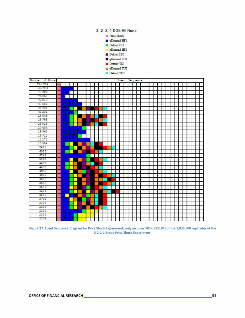
Figure 27 depicts event sequences for 935104 of the roughly 1,036,8002 realizations (~90% of the total runs) of the 3-2-2-1 Model in the Broad Price Shock Experiment3. One can see that ~ 26% of the time (269264 realizations of the model), the price shock did not result in any qDemand events.
1 For the broad design of experiments, any time a hedge fund or trading unit experienced a qDemand event in one of its assets, it was immediately followed by a qDemand event in its other asset. This is indicated as a single event in the event sequence diagrams for the broad experiment. 2 Of the 1,036,800 realizations for the broad price shock experiment: All 345,600 realizations of the 15% Price Shock completed. For the 10% Price Shock, 6 realizations of the 345,600 did not complete; and for the 13% Price Shock, 7454 realizations of the 345,600 (or 2.16% of them) did not complete. 3 Only showing the top 90% of the event sequences for illustration purposes.
OFFICE OF FINANCIAL RESEARCH 31
Figure 27: Event Sequence Diagram for Price Shock Experiment; only includes 90% (935104) of the 1,036,800 replicates of the 3-2-2-1 Broad Price Shock Experiment.
OFFICE OF FINANCIAL RESEARCH 32
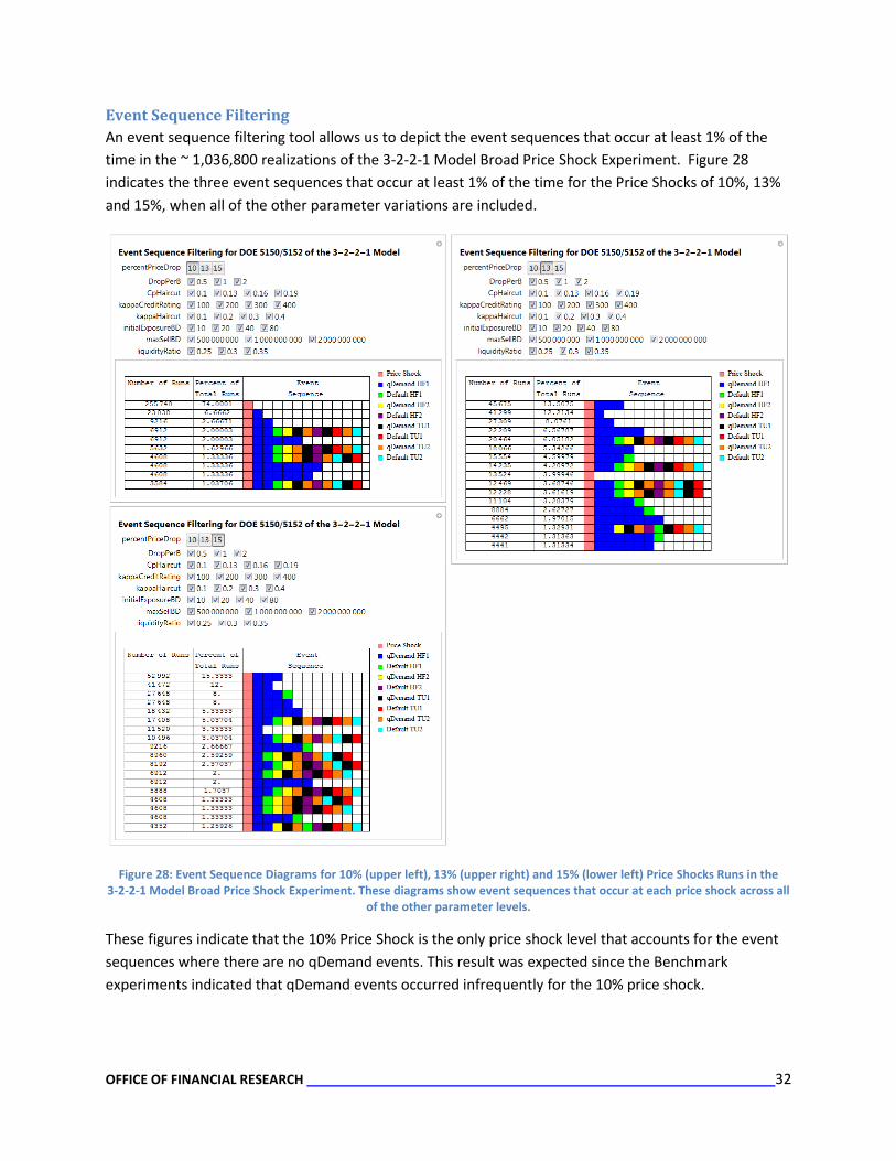
Event Sequence Filtering An event sequence filtering tool allows us to depict the event sequences that occur at least 1% of the time in the ~ 1,036,800 realizations of the 3-2-2-1 Model Broad Price Shock Experiment. Figure 28 indicates the three event sequences that occur at least 1% of the time for the Price Shocks of 10%, 13% and 15%, when all of the other parameter variations are included.
Figure 28: Event Sequence Diagrams for 10% (upper left), 13% (upper right) and 15% (lower left) Price Shocks Runs in the 3-2-2-1 Model Broad Price Shock Experiment. These diagrams show event sequences that occur at each price shock across all
of the other parameter levels.
These figures indicate that the 10% Price Shock is the only price shock level that accounts for the event sequences where there are no qDemand events. This result was expected since the Benchmark experiments indicated that qDemand events occurred infrequently for the 10% price shock.
OFFICE OF FINANCIAL RESEARCH 33
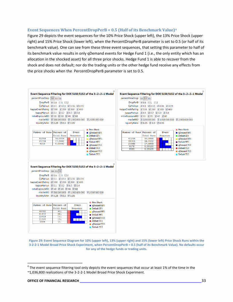
Event Sequences When PercentDropPerB = 0.5 (Half of its Benchmark Value)4 Figure 29 depicts the event sequences for the 10% Price Shock (upper left), the 13% Price Shock (upper right) and 15% Price Shock (lower left), when the PercentDropPerB parameter is set to 0.5 (or half of its benchmark value). One can see from these three event sequences, that setting this parameter to half of its benchmark value results in only qDemand events for Hedge Fund 1 (i.e., the only entity which has an allocation in the shocked asset) for all three price shocks. Hedge Fund 1 is able to recover from the shock and does not default; nor do the trading units or the other hedge fund receive any effects from the price shocks when the PercentDropPerB parameter is set to 0.5.
Figure 29: Event Sequence Diagram for 10% (upper left), 13% (upper right) and 15% (lower left) Price Shock Runs within the 3-2-2-1 Model Broad Price Shock Experiment, when PercentDropPerB = 0.5 (half of its Benchmark Value). No defaults occur
for any of the hedge funds or trading units.
4 The event sequence filtering tool only depicts the event sequences that occur at least 1% of the time in the ~1,036,800 realizations of the 3-2-2-1 Model Broad Price Shock Experiment.

OFFICE OF FINANCIAL RESEARCH 34
Event Sequences When PercentDropPerB = 1.0 (Its Benchmark Value)5 Figure 30 depicts the event sequences for the 10% Price Shock (upper left), the 13% Price Shock (upper right) and 15% Price Shock (lower left), when the PercentDropPerB parameter is set to 1.0 (its benchmark value).
Figure 32: Event Sequence Diagram for 10% (upper left), 13% (upper right) and 15% (lower left) Price Shock Runs within the 3-2-2-1 Model Broad Price Shock Experiment, when PercentDropPerB = 1.0 (the Benchmark Value).
For a 10% Price Shock, setting the benchmark value of 1.0 for the PercentDropPerB has no effect the majority of the time: 74% of the runs resulted in just a price shock event. In 20% of the runs, Hedge Fund 1 only experiences qDemand events. In 6% of the runs, Hedge Fund 1 defaults and in 2% of those runs Hedge Fund 2 has some qDemand events.
5 The event sequence filtering tool only depicts the event sequences that occur at least 1% of the time in the ~1,036,800 realizations of the 3-2-2-1 Model Broad Price Shock Experiment.

OFFICE OF FINANCIAL RESEARCH 35
For the 13% Price Shock, setting the benchmark value of 1.0 for the PercentDropPerB has no effect in almost 4% of the runs. For 50% of the runs, Hedge Fund 1 experiences only qDemand events, while another 41% of the runs results in Hedge Fund 1 defaulting. Of this latter 41%, 6% of the time, Hedge Fund 2 also experiences qDemand events; and 2% of the time everyone (i.e., both hedge funds and both trading units) experiences defaults.
A 15% Price Shock in conjunction with the PercentDropPerB setting of 1.0 always results in Hedge Fund 1 qDemand events – unlike the 10% and 13% Price Shock runs, there are no runs where the price shock has no effect. In 38% of the runs, Hedge Fund 1 only experiences qDemand events and in 48% of the runs, Hedge Fund 1 defaults. In over 3% of the runs, the other hedge fund and the trading units default.
Event Sequences When PercentDropPerB = 2.0 (Double its Benchmark Value)6
Figure 30 depicts the event sequences for the 10% Price Shock (upper left), the 13% Price Shock (upper right) and 15% Price Shock (lower left), when the PercentDropPerB parameter is set to 2.0 (double its benchmark value).
For the 10% Price Shock runs, setting the PercentDropPerB to double its benchmark value, still has little effect overall – the majority of the runs (74%) still end up with only a price shock event. However, for those runs where the price shock of 10% does result in Hedge Fund 1 experiencing qDemand events, Hedge Fund 1 also defaults and so do the second hedge fund and the trading units.
For the 13% Price Shock runs, only 4% of the runs end up with just a price shock event when the PercentDropPerB is set to double its benchmark value. In the remaining runs, not only does Hedge Fund 1 default but the other hedge fund and trading units also default.
For the 15% Price Shock runs, setting the PercentDropPerB to 2.0 always results in defaults for not only Hedge Fund 1, but also for the second hedge fund and the trading units.
Thus the larger price shocks and the large PercentDropPerB have very strong effects in the model. In fact these two parameters – the price shock and the PercentDropPerB – have such a major effect on the results that the effects of the other parameters are washed out.
6 The event sequence filtering tool only depicts the event sequences that occur at least 1% of the time in the ~1,036,800 realizations of the 3-2-2-1 Model Broad Price Shock Experiment.

OFFICE OF FINANCIAL RESEARCH 36
Figure 32: Event Sequence Diagram for 10% (upper left), 13% (upper right) and 15% (lower left) Price Shock Runs within the 3-2-2-1 Model Broad Price Shock Experiment, when PercentDropPerB = 2.0 (double its Benchmark Value).

OFFICE OF FINANCIAL RESEARCH 37
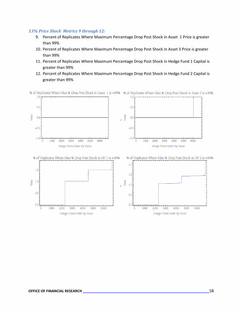
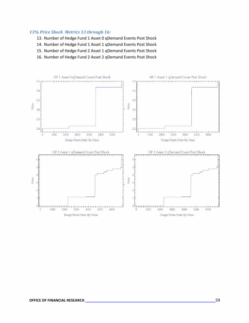
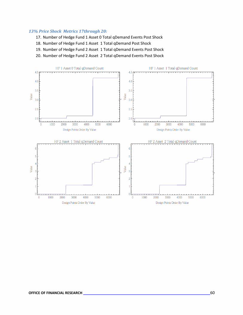
Metrics of Interest Metrics of interest defined for the 3-2-2-1 Model were:
1. Maximum Percentage Drop Post Shock in Asset 0 Price (where drop is less than or equal to 99%) 2. Maximum Percentage Drop Post Shock in Asset 1 Price (where drop is less than or equal to 99%) 3. Maximum Percentage Drop Post Shock in Asset 2 Price (where drop is less than or equal to 99%) 4. Maximum Percentage Drop Post Shock in Hedge Fund 1 Capital (where drop is less than or equal
to 99%) 5. Maximum Percentage Drop Post Shock in Hedge Fund 2 Capital (where drop is less than or equal
to 99%) 6. Percent of Replicates Where Metrics 1 through 5 are greater than 10% 7. Percent of Replicates Where Metrics 1 through 5 are greater than 20% 8. Percent of Replicates Where Maximum Percentage Drop Post Shock in Asset 0 Price is greater
than 99% 9. Percent of Replicates Where Maximum Percentage Drop Post Shock in Asset 1 Price is greater
than 99% 10. Percent of Replicates Where Maximum Percentage Drop Post Shock in Asset 3 Price is greater
than 99% 11. Percent of Replicates Where Maximum Percentage Drop Post Shock in Hedge Fund 1 Capital is
greater than 99% 12. Percent of Replicates Where Maximum Percentage Drop Post Shock in Hedge Fund 2 Capital is
greater than 99% 13. Number of Hedge Fund 1 Asset 0 qDemand Events Post Shock 14. Number of Hedge Fund 1 Asset 1 qDemand Events Post Shock 15. Number of Hedge Fund 2 Asset 1 qDemand Events Post Shock 16. Number of Hedge Fund 2 Asset 2 qDemand Events Post Shock 17. Number of Hedge Fund 1 Asset 0 Total qDemand Events Post Shock 18. Number of Hedge Fund 1 Asset 1 Total qDemand Post Shock 19. Number of Hedge Fund 2 Asset 1 Total qDemand Events Post Shock 20. Number of Hedge Fund 2 Asset 2 Total qDemand Events Post Shock 21. Hedge Fund 1 Asset 0 Mean Size of qDemand Events 22. Hedge Fund 1 Asset 1 Mean Size of qDemand Events 23. Hedge Fund 2 Asset 1 Mean Size of qDemand Events 24. Hedge Fund 2 Asset 2 Mean Size of qDemand Events 25. Total Number of Hedge Fund qDemand Defaults 26. Total Number of Trading Unit qDemand Defaults
These metrics are consistent with the results presented in the event sequences: plots of these metrics for each price shock level (10%, 13%, and 15%) display a very strong relationship with the three values for the PercentDropPerB (0.5, 1.0, 2.0). This relationship is indicated by the stair-step function depicted in these plots (see pages 50 through 71). The only metric that showed any real significant variation was

OFFICE OF FINANCIAL RESEARCH 38
Metric 26: The Total Number of Trading Unit qDemand Defaults. This is illustrated in greater detail in the next section.
Heat maps of Parameter Effects in the Broad Price Shock Experiment Since the only metric that showed any amount of variation across the design points was Metric 26: The Total Number of Trading Unit Defaults, we shall focus on that metric. We provide a heat map of the metric for the 15% Price Shock, since the 15% price shock event sequences showed the most variation.
Figures 33 displays an Array of Array Heat map for the 15% Price Shock runs. This figure depicts the Total Number of Trading Unit Defaults in a heat map construct, where no defaults are assigned a white color and the largest number of Trading Unit Defaults (i.e., 2) receives a black color. Shades between the white and black colors indicate values between 0 and 2. This heat map shows all of the runs for the given price shock and displays the levels of the other parameters within them.
Figure 33: Array of Array Heat map of the Total Number of Trading Unit Defaults for the 15% Price Shock Runs within the 3-2-2-1 Model Broad Price Shock Experiment. This heat map illustrates that the PercentDropPerB is the main driver for the
difference in the number of trading unit defaults. There are slight effects from the Max_Sell for the Bank Dealers and the Liquidity Ratio Variables as highlighted by the red boxes.
Figure 33 highlights the fact that the PercentDropPerB has a very strong effect on this metric and overwhelms the effects from the other parameters. Highlighted in red squares in this figure are the other parameter settings that have slight variations in their values: the liquidity ratio variables and the

OFFICE OF FINANCIAL RESEARCH 39
Max_Sell for the bank dealers. One needs to look really closely to discern that these other variables have slight gradations within their cells.
We shall look more closely at these variables by displaying them in individual heat maps.
Figure 34 depicts a heat map of the 15 % price shock runs with the PercentDropPerB (in the rows) and the Liquidity Ratio Variables (in the columns) as the main variables. This heat map illustrates the very strong effect from the PercentDropPerB parameter, where its highest level of 2 results in the maximum number of trading unit defaults and this holds true across every mix of the other variables and its lowest level of 0.5 results in no trading unit defaults.
Figure 34: Heat map of the Total Number of Trading Unit Defaults for the 15% Price Shock Runs within the 3-2-2-1 Model Broad Price Shock Experiment. Main variables are the PercentDropPerB (in the rows) and the Liquidity Ratio Variables (in the
columns).
The benchmark value of 1.0 for PercentDropPerB allows one to see the effects of the other main variable in this heat map – the liquidity ratios – in the middle row. Here one can see that the lowest values for the liquidity ratios result in more trading unit defaults (though the number is still less than 0.5) and the higher values for the liquidity ratios result in far fewer trading unit defaults. Thus higher

OFFICE OF FINANCIAL RESEARCH 40
liquidity has a mitigating effect on the number of trading unit defaults – as would be expected. Within the individual red squares of the middle row of the heat map, one can see that another parameter or parameters also has a slight effect due to the gradations within the squares – particularly within the middle box and far right box of the middle row.
Similarly, Figure 35 depicts a heat map of the 15 % price shock runs with the PercentDropPerB (in the rows) and the Max Sell for the Bank Dealers (in the columns) as the main variables. This heat map also illustrates the very strong effect from the PercentDropPerB parameter, where its highest level of 2 results in the maximum number of trading unit defaults and this holds true across every mix of the other variables and its lowest level of 0.5 results in no trading unit defaults. The benchmark value of 1.0 for PercentDropPerB allows one to see the effects of the other main variable in this heat map – the Max sell of the Bank Dealers – in the middle row. Here one can see that the lowest values for the Bank Dealers’ Max Sell result in more trading unit defaults (though the number is still far less than 0.5), while the higher values for the Bank Dealers’ Max Sell result in very few trading unit defaults. Within the individual red squares of the middle row of the heat map, one can see that another parameter or parameters also has a slight effect due to the gradations within the squares.
Figure 35: Heat map of the Total Number of Trading Unit Defaults for the 15% Price Shock Runs within the 3-2-2-1 Model Broad Price Shock Experiment. Main variables are the PercentDropPerB (in the rows) and the Max Sell for the Bank Dealers
(in the columns).

OFFICE OF FINANCIAL RESEARCH 41
Heat maps: Fixing the Price Shock and PercentDropPerB Levels As we have seen in the event sequences and the heat maps, the price shock levels and the PercentDropPerB levels are the main drivers of the behavior in the Broad Price Shock Experiment. In order to take a closer look at the effects of some of the other parameters, we created a series of heat maps for the 13% and 15% price shock runs that also fix the PercentDropPerB at either its benchmark level of 1.0 or at a level of 2.0 (double its benchmark value.)7
Figure 36 depicts an array of array heat map for the runs where the Price Shock level is set to 15% and the PercentDropPerB level is set to its benchmark value of 1.0. This figure displays the average of the Total Number of Trading Unit Defaults in a heat map construct where no defaults is assigned a white color and the largest average number of Trading Unit Defaults for this subset of runs receives a black color. Shades in between these two colors indicate values between 0 and the largest value (i.e., 0.36). This heat map shows all of the runs for the given price shock and displays the levels of the other parameters within them.
Figure 36: Array of Array Heat map of the Total Number of Trading Unit Defaults for the runs that have a 15% Price Shock and PercentDropPerB = 1.0 (its benchmark value) within the 3-2-2-1 Model Broad Price Shock Experiment.
7 A level of 0.5 for the PercentDropPerB resulted in just price shock events and a few qDemand events for Hedge Fund 1, which always recovered from the shock. Hence we did not create heat maps for this situation. Further, since the 10% price shock runs resulted in just a few events of interest only when the PercentDropPerB = 2.0, we did not create specialized heat maps for the 10% price shock either.

OFFICE OF FINANCIAL RESEARCH 42
In this figure, one can easily see the effects of the liquidity ratio variables and the Max Sell of the Bank Dealers. Additionally, one can start to see the small effects of the kappa credit rating, kappa haircut, and the initial Exposure Percentage for the Bank Dealers. The CP_Haircut levels also have a very small effect though it is difficult to see that very well in this heat map.
Figure 37 depicts an array of array heat map for the runs where the Price Shock level is set to 13% and the PercentDropPerB level is set to its benchmark value of 1.0. This figure displays the average of the Total Number of Trading Unit Defaults in a heat map construct where no defaults is assigned a white color and the largest average number of Trading Unit Defaults for this subset of runs receives a black color. Shades in between these two colors indicate values between 0 and this largest value (i.e., 0.12). This heat map shows all of the runs for the given price shock and displays the levels of the other parameters within them.
In this figure, one can easily see the effects of the liquidity ratio variables and the Max Sell of the Bank Dealers. Additionally, the effects of the kappa credit rating, kappa haircut, and the initial Exposure Percentage for the Bank Dealers are easily seen. The effects of the CP_Haircut levels also can be seen in this heat map.
Figure 37: Array of Array Heat map of the Total Number of Trading Unit Defaults for the runs with a 13% Price Shock and PercentDropPerB = 1.0 (its benchmark value) within the 3-2-2-1 Model Broad Price Shock Experiment.
OFFICE OF FINANCIAL RESEARCH 43
An array of array heat map of the Total Number of Trading Unit Defaults for the Price Shocks of 15% when the PercentDropPerB is set to double its benchmark value (i.e., set equal to 2.0) did not show anything interesting as both trading units always default. Similarly, since a setting of 2.0 for the PercentDropPerB results in trading unit defaults for the 13% Price Shock runs in all but 4% of the runs, an array of array heat map of the Total Number of Trading Unit Defaults also is not interesting.
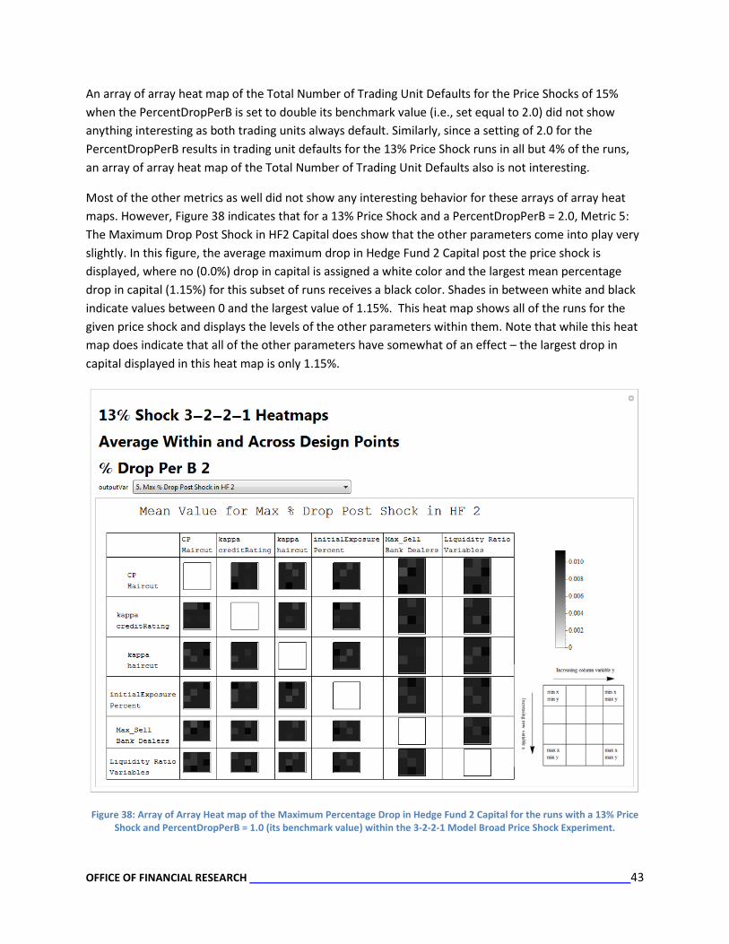
Most of the other metrics as well did not show any interesting behavior for these arrays of array heat maps. However, Figure 38 indicates that for a 13% Price Shock and a PercentDropPerB = 2.0, Metric 5: The Maximum Drop Post Shock in HF2 Capital does show that the other parameters come into play very slightly. In this figure, the average maximum drop in Hedge Fund 2 Capital post the price shock is displayed, where no (0.0%) drop in capital is assigned a white color and the largest mean percentage drop in capital (1.15%) for this subset of runs receives a black color. Shades in between white and black indicate values between 0 and the largest value of 1.15%. This heat map shows all of the runs for the given price shock and displays the levels of the other parameters within them. Note that while this heat map does indicate that all of the other parameters have somewhat of an effect – the largest drop in capital displayed in this heat map is only 1.15%.
Figure 38: Array of Array Heat map of the Maximum Percentage Drop in Hedge Fund 2 Capital for the runs with a 13% Price Shock and PercentDropPerB = 1.0 (its benchmark value) within the 3-2-2-1 Model Broad Price Shock Experiment.

OFFICE OF FINANCIAL RESEARCH 44
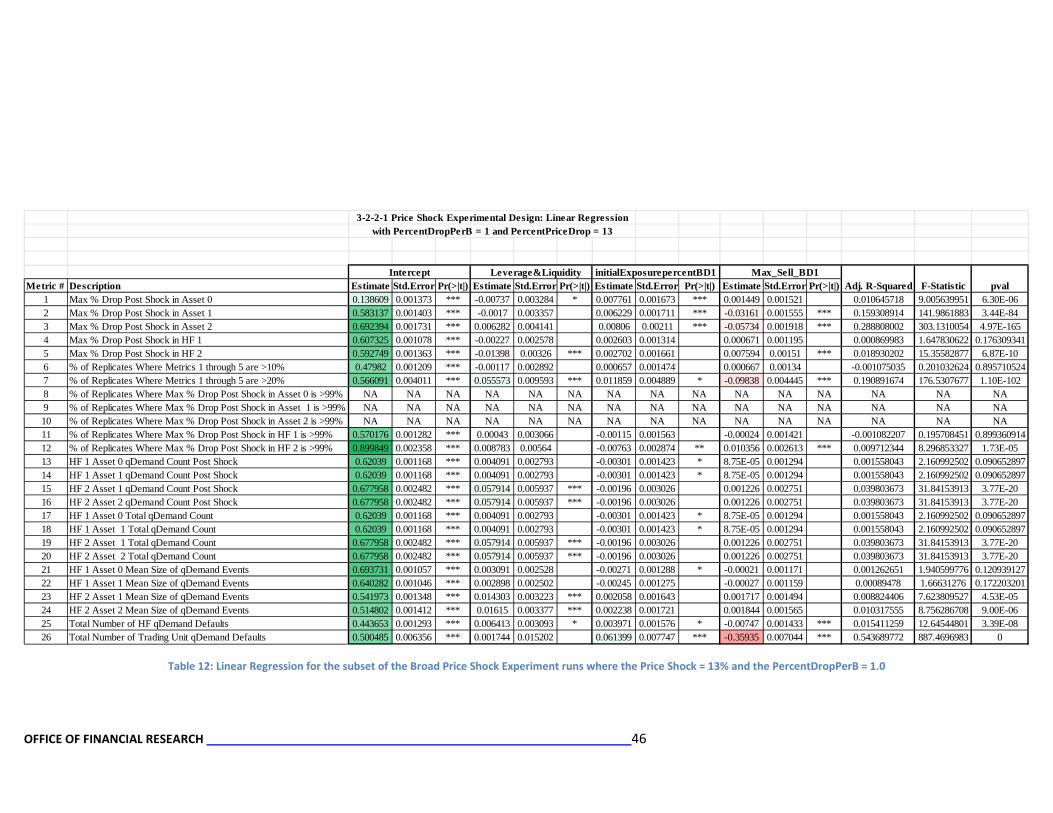
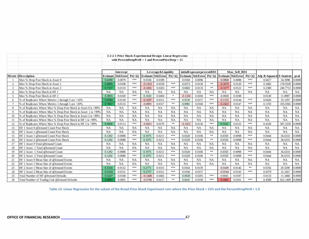
Regression Results for Broad Price Shock Experiment Linear regression results for the broad price shock experiment (see Table 11) are consistent with what we have seen in the event sequence diagrams and heat maps from the previous sections - the price shock and the PercentDropPerB are the main drivers of the variability in the runs.
Since effects from the other parameters are washed out in the regression, we conducted regressions for each of the price shocks when the PercentDropPerB was set at its Benchmark value of 1.08. For these regressions, we also combined the leverage-related and liquidity related parameters9, because even though the values of these parameters are set independently from each other, their impact on the system, i.e. their functional form within the simulation, is not independent. They all affect the resilience of the entities to the effects of price shocks. The linear regressions for the 13% and 15 % shock (depicted in Tables 12 and 13, respectively) are consistent with the results depicted in previous sections of this document. However, as indicated by the adjusted R-squares, these regressions capture little of the variation in the runs. Moreover, the F-statistics indicate these linear models are only of weak statistical significance.
8 A level of 0.5 for the PercentDropPerB resulted in just price shock events and a few qDemand events for Hedge Fund 1, which always recovered from the shock. Further, when the PercentDropPerB is double its benchmark value(i.e., is set to 2.0), the overwhelming result is that both hedge funds and the trading units default. 9 These are the CP_Haircut, kappa haircut, kappa credit rating, and liquidity ratio parameters.

OFFICE OF FINANCIAL RESEARCH 45
Table 11: Linear Regression for the Broad Price Shock Experiment conducted for the 3-2-2-1 Model
3-2-2-1 Price Shock Experimental Design: Linear Regression
Intercept PercentPriceDrop percentDropPerB CP Haircut kappa creditRating kappa haircut initialExposurePercent Max_Sell Bank Dealers Liquidity Ratio VariablesMetric # Metric Description Estimate Std.Error Pr(>|t|) Estimate Std.Error Pr(>|t|) Estimate Std.Error Pr(>|t|) Estimate Std.Error Pr(>|t|) Estimate Std.Error Pr(>|t|) Estimate Std.Error Pr(>|t|) Estimate Std.Error Pr(>|t|) Estimate Std.Error Pr(>|t|) Estimate Std.Error Pr(>|t|)
1 Max % Drop Post Shock in Asset 0 -0.1159 0.0027 *** 0.5201 0.0019 *** 0.5408 0.0018 *** 0.0000 0.0021 0.0007 0.0021 0.0008 0.0021 -0.0001 0.0020 -0.0003 0.0018 -0.0012 0.00192 Max % Drop Post Shock in Asset 1 -0.1685 0.0035 *** 0.3570 0.0024 *** 0.6722 0.0024 *** -0.0001 0.0026 -0.0008 0.0026 0.0001 0.0026 0.0011 0.0026 -0.0036 0.0024 -0.0161 0.0024 ***3 Max % Drop Post Shock in Asset 2 -0.1434 0.0040 *** 0.2333 0.0027 *** 0.6488 0.0026 *** -0.0002 0.0030 -0.0020 0.0030 -0.0007 0.0030 0.0020 0.0029 -0.0096 0.0026 *** -0.0356 0.0027 ***4 Max % Drop Post Shock in HF 1 0.6555 0.0054 *** 0.1497 0.0037 *** -0.4826 0.0036 *** 0.0001 0.0041 0.0034 0.0041 0.0020 0.0041 -0.0019 0.0040 -0.0001 0.0036 -0.0001 0.00375 Max % Drop Post Shock in HF 2 0.6570 0.0045 *** 0.1040 0.0030 *** -0.3159 0.0030 *** 0.0000 0.0034 0.0034 0.0034 0.0013 0.0034 -0.0026 0.0033 0.0001 0.0030 0.0024 0.00316 % of Replicates Where Metrics 1 through 5 are >10% -0.2134 0.0039 *** 0.3498 0.0026 *** 0.7464 0.0026 *** -0.0001 0.0029 -0.0020 0.0029 -0.0006 0.0029 0.0019 0.0028 -0.0004 0.0026 -0.0027 0.00267 % of Replicates Where Metrics 1 through 5 are >20% -0.2336 0.0044 *** 0.3060 0.0030 *** 0.7751 0.0029 *** -0.0002 0.0033 -0.0015 0.0033 0.0003 0.0033 0.0035 0.0032 -0.0040 0.0029 -0.0083 0.0030 **8* % of Replicates Where Max % Drop Post Shock in Asset 0 is >99% NaN NaN NaN NaN NaN NaN NaN NaN NaN NaN NaN NaN NaN NaN NaN NaN NaN NaN NaN NaN NaN NaN NaN NaN NaN NaN NaN9* % of Replicates Where Max % Drop Post Shock in Asset 1 is >99% NaN NaN NaN NaN NaN NaN NaN NaN NaN NaN NaN NaN NaN NaN NaN NaN NaN NaN NaN NaN NaN NaN NaN NaN NaN NaN NaN10 % of Replicates Where Max % Drop Post Shock in Asset 2 is >99% 0.0414 0.0049 *** 0.0485 0.0033 *** 0.1567 0.0033 *** -0.0003 0.0036 -0.0009 0.0036 -0.0005 0.0036 0.0011 0.0035 -0.0328 0.0033 *** -0.1462 0.0033 ***11 % of Replicates Where Max % Drop Post Shock in HF 1 is >99% 0.1028 0.0036 *** 0.0460 0.0024 *** 0.6718 0.0024 *** 0.0001 0.0027 0.0022 0.0027 0.0014 0.0027 -0.0013 0.0026 -0.0001 0.0024 0.0000 0.002512 % of Replicates Where Max % Drop Post Shock in HF 2 is >99% -0.0502 0.0030 *** 0.1729 0.0020 *** 0.6272 0.0020 *** -0.0001 0.0022 0.0035 0.0022 0.0017 0.0022 -0.0021 0.0022 0.0015 0.0020 -0.0012 0.002113 HF 1 Asset 0 qDemand Count Post Shock 0.4734 0.0077 *** -0.0434 0.0052 *** -0.1403 0.0052 *** 0.0002 0.0058 0.0048 0.0058 0.0028 0.0058 -0.0031 0.0056 -0.0001 0.0052 -0.0002 0.005314 HF 1 Asset 1 qDemand Count Post Shock 0.4734 0.0077 *** -0.0434 0.0052 *** -0.1403 0.0052 *** 0.0002 0.0058 0.0048 0.0058 0.0028 0.0058 -0.0031 0.0056 -0.0001 0.0052 -0.0002 0.005315 HF 2 Asset 1 qDemand Count Post Shock 0.1870 0.0057 *** 0.0026 0.0038 0.0753 0.0038 *** 0.0000 0.0042 0.0068 0.0042 0.0053 0.0042 -0.0034 0.0041 0.0004 0.0038 0.0108 0.0039 **16 HF 2 Asset 2 qDemand Count Post Shock 0.1870 0.0057 *** 0.0026 0.0038 0.0753 0.0038 *** 0.0000 0.0042 0.0068 0.0042 0.0053 0.0042 -0.0034 0.0041 0.0004 0.0038 0.0108 0.0039 **17 HF 1 Asset 0 Total qDemand Count 0.4734 0.0077 *** -0.0434 0.0052 *** -0.1403 0.0052 *** 0.0002 0.0058 0.0048 0.0058 0.0028 0.0058 -0.0031 0.0056 -0.0001 0.0052 -0.0002 0.005318 HF 1 Asset 1 Total qDemand Count 0.4734 0.0077 *** -0.0434 0.0052 *** -0.1403 0.0052 *** 0.0002 0.0058 0.0048 0.0058 0.0028 0.0058 -0.0031 0.0056 -0.0001 0.0052 -0.0002 0.005319 HF 2 Asset 1 Total qDemand Count 0.1870 0.0057 *** 0.0026 0.0038 0.0753 0.0038 *** 0.0000 0.0042 0.0068 0.0042 0.0053 0.0042 -0.0034 0.0041 0.0004 0.0038 0.0108 0.0039 **20 HF 2 Asset 2 Total qDemand Count 0.1870 0.0057 *** 0.0026 0.0038 0.0753 0.0038 *** 0.0000 0.0042 0.0068 0.0042 0.0053 0.0042 -0.0034 0.0041 0.0004 0.0038 0.0108 0.0039 **21 HF 1 Asset 0 Mean Size of qDemand Events 1.1105 0.0015 *** -0.3909 0.0010 *** -0.6325 0.0010 *** 0.0000 0.0011 0.0007 0.0011 0.0004 0.0011 -0.0005 0.0011 0.0000 0.0010 -0.0001 0.001022 HF 1 Asset 1 Mean Size of qDemand Events 1.0954 0.0013 *** -0.3233 0.0009 *** -0.5925 0.0009 *** 0.0000 0.0010 0.0007 0.0010 0.0003 0.0010 -0.0005 0.0010 0.0000 0.0009 -0.0001 0.000923 HF 2 Asset 1 Mean Size of qDemand Events 1.0155 0.0014 *** -0.0986 0.0010 *** -0.5825 0.0009 *** 0.0001 0.0011 -0.0009 0.0011 -0.0003 0.0011 0.0008 0.0010 -0.0001 0.0009 0.0047 0.0010 ***24 HF 2 Asset 2 Mean Size of qDemand Events 1.0086 0.0015 *** -0.0948 0.0010 *** -0.5312 0.0010 *** 0.0001 0.0011 -0.0009 0.0011 -0.0004 0.0011 0.0008 0.0011 -0.0001 0.0010 0.0048 0.0010 ***25 Total Number of HF qDemand Defaults -0.2095 0.0037 *** 0.3786 0.0025 *** 0.7428 0.0025 *** -0.0001 0.0028 -0.0006 0.0028 0.0006 0.0028 0.0010 0.0027 0.0000 0.0025 -0.0022 0.002526 Total Number of Trading Unit qDemand Defaults -0.2285 0.0045 *** 0.2978 0.0030 *** 0.7749 0.0030 *** -0.0002 0.0033 -0.0013 0.0033 0.0003 0.0033 0.0040 0.0033 -0.0143 0.0030 *** -0.0119 0.0030 ***
OFFICE OF FINANCIAL RESEARCH 46
Table 12: Linear Regression for the subset of the Broad Price Shock Experiment runs where the Price Shock = 13% and the PercentDropPerB = 1.0
3-2-2-1 Price Shock Experimental Design: Linear Regressionwith PercentDropPerB = 1 and PercentPriceDrop = 13
Intercept Leverage&Liquidity initialExposurepercentBD1 Max_Sell_BD1Metric # Description Estimate Std.Error Pr(>|t|) Estimate Std.Error Pr(>|t|) Estimate Std.Error Pr(>|t|) Estimate Std.Error Pr(>|t|) Adj. R-Squared F-Statistic pval
1 Max % Drop Post Shock in Asset 0 0.138609 0.001373 *** -0.00737 0.003284 * 0.007761 0.001673 *** 0.001449 0.001521 0.010645718 9.005639951 6.30E-062 Max % Drop Post Shock in Asset 1 0.583137 0.001403 *** -0.0017 0.003357 0.006229 0.001711 *** -0.03161 0.001555 *** 0.159308914 141.9861883 3.44E-843 Max % Drop Post Shock in Asset 2 0.692394 0.001731 *** 0.006282 0.004141 0.00806 0.00211 *** -0.05734 0.001918 *** 0.288808002 303.1310054 4.97E-1654 Max % Drop Post Shock in HF 1 0.607325 0.001078 *** -0.00227 0.002578 0.002603 0.001314 0.000671 0.001195 0.000869983 1.647830622 0.1763093415 Max % Drop Post Shock in HF 2 0.592749 0.001363 *** -0.01398 0.00326 *** 0.002702 0.001661 0.007594 0.00151 *** 0.018930202 15.35582877 6.87E-106 % of Replicates Where Metrics 1 through 5 are >10% 0.47982 0.001209 *** -0.00117 0.002892 0.000657 0.001474 0.000667 0.00134 -0.001075035 0.201032624 0.8957105247 % of Replicates Where Metrics 1 through 5 are >20% 0.566091 0.004011 *** 0.055573 0.009593 *** 0.011859 0.004889 * -0.09838 0.004445 *** 0.190891674 176.5307677 1.10E-1028 % of Replicates Where Max % Drop Post Shock in Asset 0 is >99% NA NA NA NA NA NA NA NA NA NA NA NA NA NA NA9 % of Replicates Where Max % Drop Post Shock in Asset 1 is >99% NA NA NA NA NA NA NA NA NA NA NA NA NA NA NA10 % of Replicates Where Max % Drop Post Shock in Asset 2 is >99% NA NA NA NA NA NA NA NA NA NA NA NA NA NA NA11 % of Replicates Where Max % Drop Post Shock in HF 1 is >99% 0.570176 0.001282 *** 0.00043 0.003066 -0.00115 0.001563 -0.00024 0.001421 -0.001082207 0.195708451 0.89936091412 % of Replicates Where Max % Drop Post Shock in HF 2 is >99% 0.899849 0.002358 *** 0.008783 0.00564 -0.00763 0.002874 ** 0.010356 0.002613 *** 0.009712344 8.296853327 1.73E-0513 HF 1 Asset 0 qDemand Count Post Shock 0.62039 0.001168 *** 0.004091 0.002793 -0.00301 0.001423 * 8.75E-05 0.001294 0.001558043 2.160992502 0.09065289714 HF 1 Asset 1 qDemand Count Post Shock 0.62039 0.001168 *** 0.004091 0.002793 -0.00301 0.001423 * 8.75E-05 0.001294 0.001558043 2.160992502 0.09065289715 HF 2 Asset 1 qDemand Count Post Shock 0.677958 0.002482 *** 0.057914 0.005937 *** -0.00196 0.003026 0.001226 0.002751 0.039803673 31.84153913 3.77E-2016 HF 2 Asset 2 qDemand Count Post Shock 0.677958 0.002482 *** 0.057914 0.005937 *** -0.00196 0.003026 0.001226 0.002751 0.039803673 31.84153913 3.77E-2017 HF 1 Asset 0 Total qDemand Count 0.62039 0.001168 *** 0.004091 0.002793 -0.00301 0.001423 * 8.75E-05 0.001294 0.001558043 2.160992502 0.09065289718 HF 1 Asset 1 Total qDemand Count 0.62039 0.001168 *** 0.004091 0.002793 -0.00301 0.001423 * 8.75E-05 0.001294 0.001558043 2.160992502 0.09065289719 HF 2 Asset 1 Total qDemand Count 0.677958 0.002482 *** 0.057914 0.005937 *** -0.00196 0.003026 0.001226 0.002751 0.039803673 31.84153913 3.77E-2020 HF 2 Asset 2 Total qDemand Count 0.677958 0.002482 *** 0.057914 0.005937 *** -0.00196 0.003026 0.001226 0.002751 0.039803673 31.84153913 3.77E-2021 HF 1 Asset 0 Mean Size of qDemand Events 0.693731 0.001057 *** 0.003091 0.002528 -0.00271 0.001288 * -0.00021 0.001171 0.001262651 1.940599776 0.12093912722 HF 1 Asset 1 Mean Size of qDemand Events 0.640282 0.001046 *** 0.002898 0.002502 -0.00245 0.001275 -0.00027 0.001159 0.00089478 1.66631276 0.17220320123 HF 2 Asset 1 Mean Size of qDemand Events 0.541973 0.001348 *** 0.014303 0.003223 *** 0.002058 0.001643 0.001717 0.001494 0.008824406 7.623809527 4.53E-0524 HF 2 Asset 2 Mean Size of qDemand Events 0.514802 0.001412 *** 0.01615 0.003377 *** 0.002238 0.001721 0.001844 0.001565 0.010317555 8.756286708 9.00E-0625 Total Number of HF qDemand Defaults 0.443653 0.001293 *** 0.006413 0.003093 * 0.003971 0.001576 * -0.00747 0.001433 *** 0.015411259 12.64544801 3.39E-0826 Total Number of Trading Unit qDemand Defaults 0.500485 0.006356 *** 0.001744 0.015202 0.061399 0.007747 *** -0.35935 0.007044 *** 0.543689772 887.4696983 0
OFFICE OF FINANCIAL RESEARCH 47
Table 13: Linear Regression for the subset of the Broad Price Shock Experiment runs where the Price Shock = 15% and the PercentDropPerB = 1.0
3-2-2-1 Price Shock Experimental Design: Linear Regressionwith PercentDropPerB = 1 and PercentPriceDrop = 15
Intercept Leverage&Liquidity initialExposurepercentBD1 Max_Sell_BD1Metric #Description Estimate Std.Error Pr(>|t|) Estimate Std.Error Pr(>|t|) Estimate Std.Error Pr(>|t|) Estimate Std.Error Pr(>|t|) Adj. R-Squared F-Statistic pval
1 Max % Drop Post Shock in Asset 0 0.4290 0.0079 *** 0.0336 0.0189 0.0160 0.0096 -0.0868 0.0088 *** 0.0417 34.3998 0.00002 Max % Drop Post Shock in Asset 1 0.6805 0.0108 *** -0.1433 0.0258 *** 0.0373 0.0130 ** -0.2676 0.0120 *** 0.1882 178.9339 0.00003 Max % Drop Post Shock in Asset 2 0.7337 0.0110 *** -0.1601 0.0263 *** 0.0402 0.0133 ** -0.3177 0.0122 *** 0.2380 240.7712 0.00004 Max % Drop Post Shock in HF 1 NA NA NA NA NA NA NA NA NA NA NA NA NA NA NA5 Max % Drop Post Shock in HF 2 0.3855 0.0169 *** 0.1020 0.0404 * -0.1104 0.0204 *** -0.0040 0.0188 0.0140 11.8987 0.00006 % of Replicates Where Metrics 1 through 5 are >10% 0.6984 0.0130 *** -0.1697 0.0311 *** 0.0530 0.0157 *** -0.1155 0.0144 *** 0.0426 35.1297 0.00007 % of Replicates Where Metrics 1 through 5 are >20% 0.7847 0.0133 *** -0.0891 0.0317 ** 0.0981 0.0160 *** -0.2422 0.0147 *** 0.1193 105.0365 0.00008 % of Replicates Where Max % Drop Post Shock in Asset 0 is >99% NA NA NA NA NA NA NA NA NA NA NA NA NA NA NA9 % of Replicates Where Max % Drop Post Shock in Asset 1 is >99% NA NA NA NA NA NA NA NA NA NA NA NA NA NA NA10 % of Replicates Where Max % Drop Post Shock in Asset 2 is >99% NA NA NA NA NA NA NA NA NA NA NA NA NA NA NA11 % of Replicates Where Max % Drop Post Shock in HF 1 is >99% NA NA NA NA NA NA NA NA NA NA NA NA NA NA NA12 % of Replicates Where Max % Drop Post Shock in HF 2 is >99% 0.4926 0.0113 *** -0.0825 0.0270 ** -0.1023 0.0136 *** 0.5162 0.0125 *** 0.4330 587.2259 0.000013 HF 1 Asset 0 qDemand Count Post Shock NA NA NA NA NA NA NA NA NA NA NA NA NA NA NA14 HF 1 Asset 1 qDemand Count Post Shock NA NA NA NA NA NA NA NA NA NA NA NA NA NA NA15 HF 2 Asset 1 qDemand Count Post Shock 0.1292 0.0088 *** 0.1975 0.0211 *** 0.0320 0.0106 ** 0.0350 0.0098 *** 0.0444 36.6333 0.000016 HF 2 Asset 2 qDemand Count Post Shock 0.1292 0.0088 *** 0.1975 0.0211 *** 0.0320 0.0106 ** 0.0350 0.0098 *** 0.0444 36.6333 0.000017 HF 1 Asset 0 Total qDemand Count NA NA NA NA NA NA NA NA NA NA NA NA NA NA NA18 HF 1 Asset 1 Total qDemand Count NA NA NA NA NA NA NA NA NA NA NA NA NA NA NA19 HF 2 Asset 1 Total qDemand Count 0.1292 0.0088 *** 0.1975 0.0211 *** 0.0320 0.0106 ** 0.0350 0.0098 *** 0.0444 36.6333 0.000020 HF 2 Asset 2 Total qDemand Count 0.1292 0.0088 *** 0.1975 0.0211 *** 0.0320 0.0106 ** 0.0350 0.0098 *** 0.0444 36.6333 0.000021 HF 1 Asset 0 Mean Size of qDemand Events NA NA NA NA NA NA NA NA NA NA NA NA NA NA NA22 HF 1 Asset 1 Mean Size of qDemand Events NA NA NA NA NA NA NA NA NA NA NA NA NA NA NA23 HF 2 Asset 1 Mean Size of qDemand Events 0.5316 0.0132 *** 0.2771 0.0315 *** 0.0164 0.0159 -0.0449 0.0146 ** 0.0356 29.3290 0.000024 HF 2 Asset 2 Mean Size of qDemand Events 0.5334 0.0131 *** 0.2757 0.0311 *** 0.0166 0.0157 -0.0544 0.0145 *** 0.0379 31.2267 0.000025 Total Number of HF qDemand Defaults 0.5437 0.0168 *** -0.1448 0.0402 *** 0.0928 0.0203 *** 0.0045 0.0187 0.0133 11.3460 0.000026 Total Number of Trading Unit qDemand Defaults 0.8892 0.0091 *** -0.0708 0.0217 ** 0.0641 0.0109 *** -0.4401 0.0101 *** 0.4589 652.1409 0.0000

OFFICE OF FINANCIAL RESEARCH 48
Metric Plots for Broad Price Shock Experiment The metric plots order the design points by the metric value and plot them against the metric value for the individual metric. Metric Plots were created for each Price Shock level within the Broad Price Shock Experiment. For each price shock level, there were 6912 design points.
The metric plots for each price shock level (10%, 13%, and 15%) display a very strong relationship with the three values for the PercentDropPerB (0.5, 1.0, and 2.0). This relationship is indicated by the stair-step function depicted in the majority of these plots. The first one-third (or 2304) of the ordered design points correspond to the PercentDropPerB value of 0.5 (half of its benchmark value); the second one-third of the design points correspond to the PercentDropPerB value of 1.0 (the benchmark value); and the final one-third of the ordered design points correspond to the PercentDropPerB value of 2.0 (double its benchmark value). An example of this is shown in Figure 39 – where boxes indicating the PercentDropPerB levels are superimposed on a metric plot.
Low Level for PercentPerB
Medium Level for PercentPerB
High Level for PercentPerB
Figure 39: Example of Strong Relationship between Design Points Ordered by Metric Value and the PercentDropPerB Levels
The following sections provide the metric plots for each of the Price Shock levels within the 3-2-2-1 Model Broad Price Experiment.

OFFICE OF FINANCIAL RESEARCH 49
10% Shock Metric Plots
10% Price Shock Metrics 1through 4: 1. Maximum Percentage Drop Post Shock in Asset 0 Price (where drop is less than or equal to 99%) 2. Maximum Percentage Drop Post Shock in Asset 1 Price (where drop is less than or equal to 99%) 3. Maximum Percentage Drop Post Shock in Asset 2 Price (where drop is less than or equal to 99%) 4. Maximum Percentage Drop Post Shock in Hedge Fund 1 Capital (where drop is less than or equal
to 99%)
OFFICE OF FINANCIAL RESEARCH 50
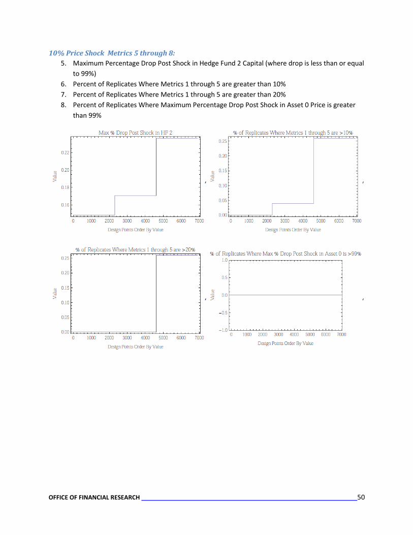
10% Price Shock Metrics 5 through 8: 5. Maximum Percentage Drop Post Shock in Hedge Fund 2 Capital (where drop is less than or equal
to 99%) 6. Percent of Replicates Where Metrics 1 through 5 are greater than 10% 7. Percent of Replicates Where Metrics 1 through 5 are greater than 20% 8. Percent of Replicates Where Maximum Percentage Drop Post Shock in Asset 0 Price is greater
than 99%
OFFICE OF FINANCIAL RESEARCH 51
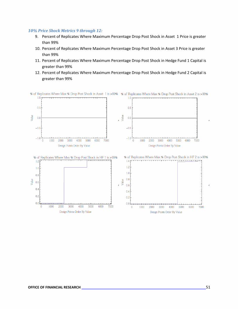
10% Price Shock Metrics 9 through 12: 9. Percent of Replicates Where Maximum Percentage Drop Post Shock in Asset 1 Price is greater
than 99% 10. Percent of Replicates Where Maximum Percentage Drop Post Shock in Asset 3 Price is greater
than 99% 11. Percent of Replicates Where Maximum Percentage Drop Post Shock in Hedge Fund 1 Capital is
greater than 99% 12. Percent of Replicates Where Maximum Percentage Drop Post Shock in Hedge Fund 2 Capital is
greater than 99%
OFFICE OF FINANCIAL RESEARCH 52
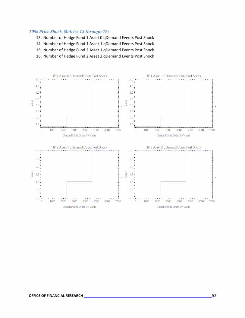
10% Price Shock Metrics 13 through 16: 13. Number of Hedge Fund 1 Asset 0 qDemand Events Post Shock 14. Number of Hedge Fund 1 Asset 1 qDemand Events Post Shock 15. Number of Hedge Fund 2 Asset 1 qDemand Events Post Shock 16. Number of Hedge Fund 2 Asset 2 qDemand Events Post Shock
OFFICE OF FINANCIAL RESEARCH 53
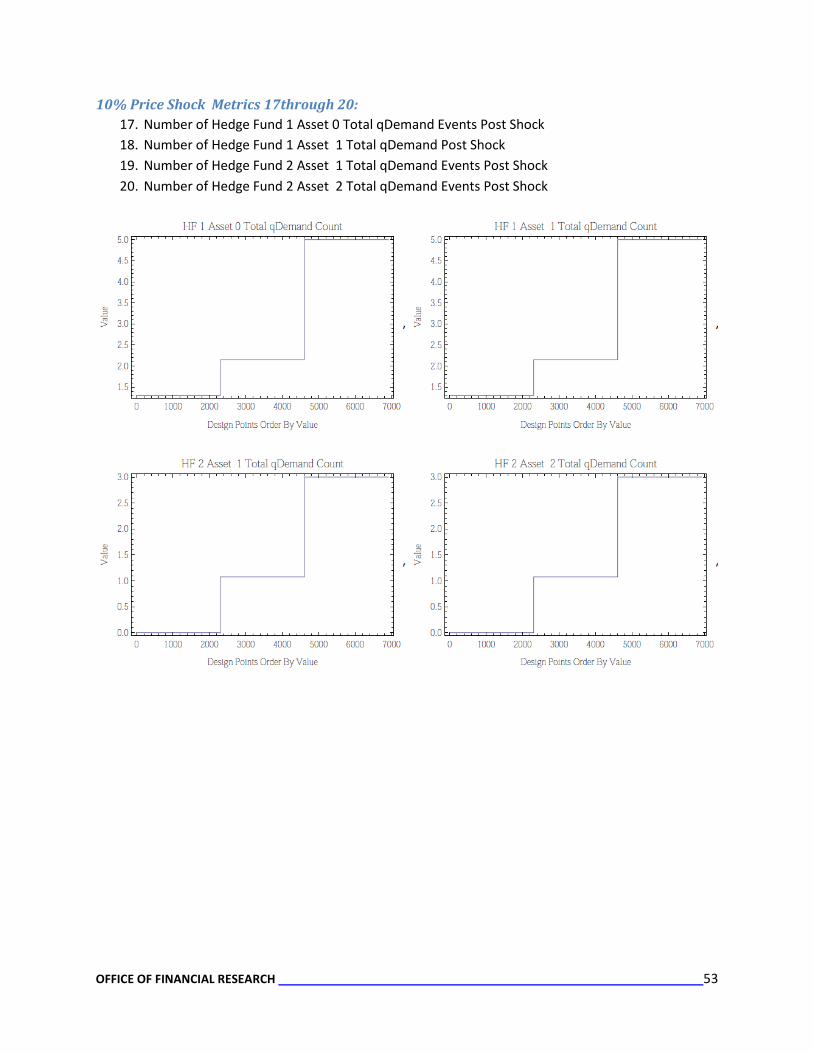
10% Price Shock Metrics 17through 20: 17. Number of Hedge Fund 1 Asset 0 Total qDemand Events Post Shock 18. Number of Hedge Fund 1 Asset 1 Total qDemand Post Shock 19. Number of Hedge Fund 2 Asset 1 Total qDemand Events Post Shock 20. Number of Hedge Fund 2 Asset 2 Total qDemand Events Post Shock

OFFICE OF FINANCIAL RESEARCH 54
10% Price Shock Metrics 21 through 24: 21. Hedge Fund 1 Asset 0 Mean Size of qDemand Events 22. Hedge Fund 1 Asset 1 Mean Size of qDemand Events 23. Hedge Fund 2 Asset 1 Mean Size of qDemand Events 24. Hedge Fund 2 Asset 2 Mean Size of qDemand Events
OFFICE OF FINANCIAL RESEARCH 55
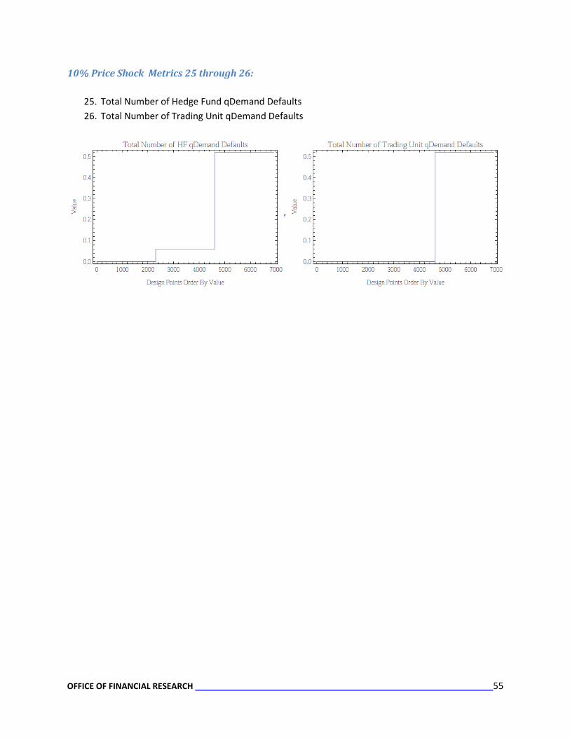
10% Price Shock Metrics 25 through 26:
25. Total Number of Hedge Fund qDemand Defaults 26. Total Number of Trading Unit qDemand Defaults

OFFICE OF FINANCIAL RESEARCH 56
13% Shock Metric Plots
13% Price Shock Metrics 1through 4: 1. Maximum Percentage Drop Post Shock in Asset 0 Price (where drop is less than or equal to 99%) 2. Maximum Percentage Drop Post Shock in Asset 1 Price (where drop is less than or equal to 99%) 3. Maximum Percentage Drop Post Shock in Asset 2 Price (where drop is less than or equal to 99%) 4. Maximum Percentage Drop Post Shock in Hedge Fund 1 Capital (where drop is less than or equal
to 99%)

OFFICE OF FINANCIAL RESEARCH 57
13% Price Shock Metrics 5 through 8: 5. Maximum Percentage Drop Post Shock in Hedge Fund 2 Capital (where drop is less than or equal
to 99%) 6. Percent of Replicates Where Metrics 1 through 5 are greater than 10% 7. Percent of Replicates Where Metrics 1 through 5 are greater than 20% 8. Percent of Replicates Where Maximum Percentage Drop Post Shock in Asset 0 Price is greater
than 99%
OFFICE OF FINANCIAL RESEARCH 58
13% Price Shock Metrics 9 through 12: 9. Percent of Replicates Where Maximum Percentage Drop Post Shock in Asset 1 Price is greater
than 99% 10. Percent of Replicates Where Maximum Percentage Drop Post Shock in Asset 3 Price is greater
than 99% 11. Percent of Replicates Where Maximum Percentage Drop Post Shock in Hedge Fund 1 Capital is
greater than 99% 12. Percent of Replicates Where Maximum Percentage Drop Post Shock in Hedge Fund 2 Capital is
greater than 99%
OFFICE OF FINANCIAL RESEARCH 59
13% Price Shock Metrics 13 through 16: 13. Number of Hedge Fund 1 Asset 0 qDemand Events Post Shock 14. Number of Hedge Fund 1 Asset 1 qDemand Events Post Shock 15. Number of Hedge Fund 2 Asset 1 qDemand Events Post Shock 16. Number of Hedge Fund 2 Asset 2 qDemand Events Post Shock
OFFICE OF FINANCIAL RESEARCH 60
13% Price Shock Metrics 17through 20: 17. Number of Hedge Fund 1 Asset 0 Total qDemand Events Post Shock 18. Number of Hedge Fund 1 Asset 1 Total qDemand Post Shock 19. Number of Hedge Fund 2 Asset 1 Total qDemand Events Post Shock 20. Number of Hedge Fund 2 Asset 2 Total qDemand Events Post Shock

OFFICE OF FINANCIAL RESEARCH 61
13% Price Shock Metrics 21 through 24: 21. Hedge Fund 1 Asset 0 Mean Size of qDemand Events 22. Hedge Fund 1 Asset 1 Mean Size of qDemand Events 23. Hedge Fund 2 Asset 1 Mean Size of qDemand Events 24. Hedge Fund 2 Asset 2 Mean Size of qDemand Events
OFFICE OF FINANCIAL RESEARCH 62
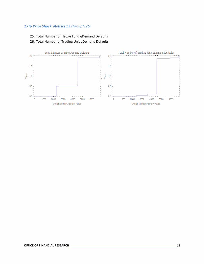
13% Price Shock Metrics 25 through 26:
25. Total Number of Hedge Fund qDemand Defaults 26. Total Number of Trading Unit qDemand Defaults

OFFICE OF FINANCIAL RESEARCH 63
15% Shock Metric Plots
15% Price Shock Metrics 1through 4: 1. Maximum Percentage Drop Post Shock in Asset 0 Price (where drop is less than or equal to 99%) 2. Maximum Percentage Drop Post Shock in Asset 1 Price (where drop is less than or equal to 99%) 3. Maximum Percentage Drop Post Shock in Asset 2 Price (where drop is less than or equal to 99%) 4. Maximum Percentage Drop Post Shock in Hedge Fund 1 Capital (where drop is less than or equal
to 99%)

OFFICE OF FINANCIAL RESEARCH 64
15% Price Shock Metrics 5 through 8: 5. Maximum Percentage Drop Post Shock in Hedge Fund 2 Capital (where drop is less than or equal
to 99%) 6. Percent of Replicates Where Metrics 1 through 5 are greater than 10% 7. Percent of Replicates Where Metrics 1 through 5 are greater than 20% 8. Percent of Replicates Where Maximum Percentage Drop Post Shock in Asset 0 Price is greater
than 99%

OFFICE OF FINANCIAL RESEARCH 65
15% Price Shock Metrics 9 through 12: 9. Percent of Replicates Where Maximum Percentage Drop Post Shock in Asset 1 Price is greater
than 99% 10. Percent of Replicates Where Maximum Percentage Drop Post Shock in Asset 3 Price is greater
than 99% 11. Percent of Replicates Where Maximum Percentage Drop Post Shock in Hedge Fund 1 Capital is
greater than 99% 12. Percent of Replicates Where Maximum Percentage Drop Post Shock in Hedge Fund 2 Capital is
greater than 99%

OFFICE OF FINANCIAL RESEARCH 66
15% Price Shock Metrics 13 through 16: 13. Number of Hedge Fund 1 Asset 0 qDemand Events Post Shock 14. Number of Hedge Fund 1 Asset 1 qDemand Events Post Shock 15. Number of Hedge Fund 2 Asset 1 qDemand Events Post Shock 16. Number of Hedge Fund 2 Asset 2 qDemand Events Post Shock

OFFICE OF FINANCIAL RESEARCH 67
15% Price Shock Metrics 17through 20: 17. Number of Hedge Fund 1 Asset 0 Total qDemand Events Post Shock 18. Number of Hedge Fund 1 Asset 1 Total qDemand Post Shock 19. Number of Hedge Fund 2 Asset 1 Total qDemand Events Post Shock 20. Number of Hedge Fund 2 Asset 2 Total qDemand Events Post Shock
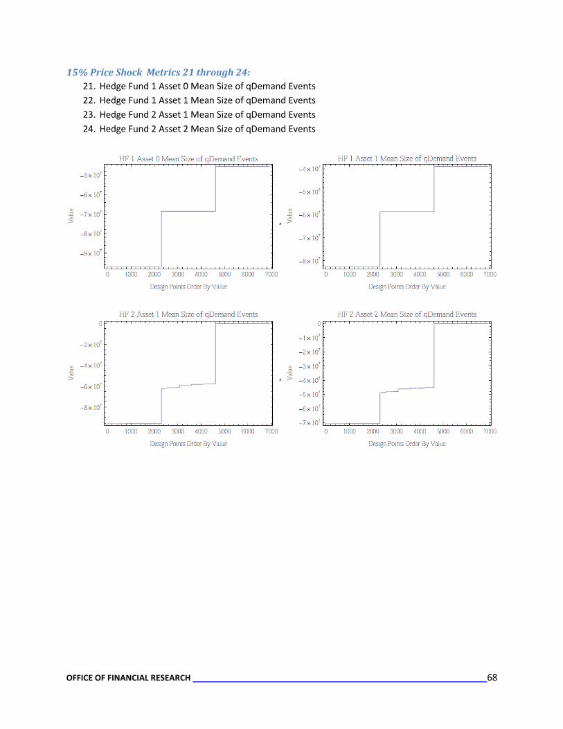
OFFICE OF FINANCIAL RESEARCH 68
15% Price Shock Metrics 21 through 24: 21. Hedge Fund 1 Asset 0 Mean Size of qDemand Events 22. Hedge Fund 1 Asset 1 Mean Size of qDemand Events 23. Hedge Fund 2 Asset 1 Mean Size of qDemand Events 24. Hedge Fund 2 Asset 2 Mean Size of qDemand Events
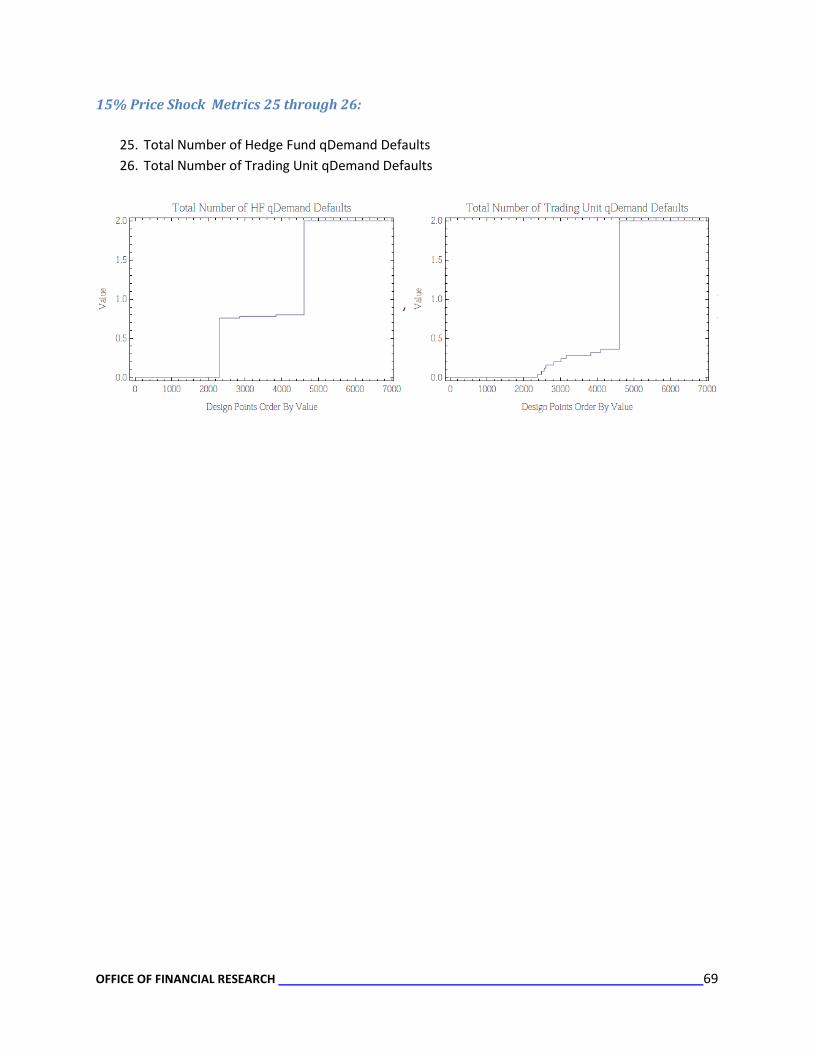
OFFICE OF FINANCIAL RESEARCH 69
15% Price Shock Metrics 25 through 26:
25. Total Number of Hedge Fund qDemand Defaults 26. Total Number of Trading Unit qDemand Defaults