Embed Size (px)
Citation preview

An AFE based Embedded System for Physiological
Computing
by
Md. Nazrul Islam Khan
A thesis submitted to the
School of Graduate and Postdoctoral Studies in partial
fulfillment of the requirements for the degree of
Doctor of Philosophy in Electrical and Computer Engineering
Department of Electrical, Computer and Software Engineering
Faculty of Engineering and Applied Science
Ontario Tech University
Oshawa, Ontario, Canada
November 2019
© Nazrul Khan, 2019

ii
THESIS EXAMINATION INFORMATION
Submitted by: Md. Nazrul Islam Khan
Doctor of Philosophy in Electrical and Computer Engineering
Thesis Title: An AFE based Embedded System for Physiological
Computing
An oral defense of this thesis took place on November 11, 2019 in front of the following
examining committee:
Examining Committee:
Chair of Examining Committee Dr. Ying Wang
Research Supervisor Dr. Mikael Eklund
Examining Committee Member Dr. Ruth Milman
Examining Committee Member Dr. Akramul Azim
University Examiner Dr. Patrick Hung
External Examiner Dr. Ana Luisa Trejos
The above committee determined that the thesis is acceptable in form and content and
that a satisfactory knowledge of the field covered by the thesis was demonstrated by the
candidate during an oral examination. A signed copy of the Certificate of Approval is
available from the School of Graduate and Postdoctoral Studies.

iii
ABSTRACT
The present hospital-based health care system will be burdened because of the
growing aging population. Aging and stress result in cardiovascular diseases that cost
around seventeen million lives globally every year. To control cardiovascular ailments, at-
home monitoring of blood pressure is very important which helps diet control and promote
medication adherence. The present health monitors are by default bulky, daunting,
invasive, and not suitable for home use. The de-facto architecture of such systems entails
discrete sensors and analog sub-systems known as the analog front end (AFE) for biosignal
acquisition, conditioning, and vital bridging function. Being discrete and analog, signal
processing is limited. Besides, with large form factor, component counts and power
consumption increase with the constant need for calibration.
For more than one century, the non‐invasive measurement of blood pressure has
relied on the inflation of pneumatic cuffs around a limb. In addition to being occlusive and
thus cumbersome, clinical cuff‐based methods, provide intermittent BP readings, hence
impeding the suitable monitoring of short‐term BP regulation mechanisms. Cuff‐based
methods may not be a true representative of BP. Therefore, the development of novel
technologies that eliminate the use of pneumatic cuffs is justified.
In this thesis, I present a highly integrated programmable AFE based biosignal
computing platform, named TasDiag. TasDiag is a novel, integrated, remote platform
capable of multimodal biosignal computing including non-invasive, continuous, and cuff-
less BP estimation based on pulse transit time. Being integrated, and digital, TasDiag is a
single board solution with an auto calibration scheme implemented through novel signal
processing and computing. The developed system is validated using real-time data from
human subjects and subjected to various statistical analyses for performance and accuracy.
Test results show TasDiag comply with the Association for Advancement for Medical
Instrumentation standard and can replace its industry-standard counterparts.
Keywords: health monitor; blood pressure; analog front end; pulse transit time; single
board computer.

iv
AUTHOR’S DECLARATION
I hereby declare that this thesis consists of original work of which I have
authored. This is a true copy of the thesis, including any required final revisions,
as accepted by my examiners.
I authorize the university of Ontario Institute of Technology to lend this
thesis to other institutions or individuals for the purpose of scholarly research. I
further authorize University of Ontario Institute Technology to reproduce this
thesis by photocopying or by other means, in total or in part, at the request of
other institutions or individuals for the purpose of scholarly research. I understand
that my thesis will be made electronically available to the public.
The research work in this thesis that was performed in compliance with
the regulations of University of Ontario Institute of Technology’s Research Ethics
Board under REB Certificate number 14522.
Md. Nazrul Islam Khan

v
STATEMENT OF CONTRIBUTIONS
Part of the work has been published as:
1. N. Khan and J. M. Eklund, “A highly Integrated Computing Platform for
continuous, non-invasive BP estimation”, IEEE Canadian conference on Electrical
and Computer Engineering (CCECE), Quebec, Canada, 2018.
2. J. M. Eklund and N. Khan, “A bio-signal computing platform for real-time online
health analytics for manned space missions”, IEEE Aerospace conference,
Montana, USA, 2018.
3. N. Khan and J. M. Eklund, "A Programmable Integrated AFE‐Based Embedded
System for Continuous, Non‐Invasive Blood Pressure Monitoring," submitted to
IEEE Transaction on Biomedical Circuits and Systems, November 2019
I performed all the testing and writing of the manuscript.

vi
DEDICATION
To my beloved father, who taught me humanity and my resilient mother,
who championed the tenants of education.

vii
ACKNOWLEDGEMENTS
Research is an undertaking to extend knowledge through a disciplined inquiry or
systematic investigation. To take such an undertaking, it requires huge personal
commitments and the active support of a team of people. For that, my heartfelt thanks to:
My advisor Dr. Mikael Eklund, for giving me total freedom for exploration. Since
the very first day of this PhD, he has encouraged me to solve the problem through critical
thinking, motivating with thoughtful ideas, supporting the useful points, and criticizing the
wrong ones. His all-out support has been the key element of the success of my thesis. His
well-reasoned and analytic view of my research has wisely guided this PhD thesis. Outside
the purview of supervision, I found him responsible, considerate, and a true gentleman with
amazing personal qualities.
My past boss, Mr. Brian Jervis, who inked his initial on my application in support
of my PhD study and my employer Sheridan College to sponsor my study partly. Dr. Farzad
Rayegani, who landed his full support for my study. My family physician, Dr. Rohit
Nagpal, who handed me a book on cardiovascular physiology after knowing my research
topic.
My colleagues Dr. Subir, Mr. Paul Kemp, Mr. Nigel Johnson, Mr. Stefan Korol,
Dr. Weijing Ma, Dr. Zohreh Motamedi and Dr. Mouhamed Abdulla for their valuable
support, expertise, and encouragement.
The support team at the Electronics lab at Sheridan College, namely Mr. Tom King,
Lawrence Porter, and others. Mr. Tom King took the extra mileage to help me out whenever
there is a need. His relentless support in providing logistics is paramount to my research.
Also, Mr. Carl Barnes and Mr. Kevin from Technological Arts for their ability in
populating the PCB.
The team of engineers at Microchip, Mr. Andre Nemat, Mr. Zhang Feng, and Mr.
Ryan Bartling for their fruitful and active support to my research. Whenever I am stuck
with the development tool or the Microcontroller, Andre Nemat was my first contact. For
any signal processing need, Zhang and Ryan always in my help. Their theoretical and

viii
practical knowledge of signal processing has undeniably guided my research work. Mr.
Hugh Dixon at Ledstar Inc., and Mr. Don Jackson at Labcenter, who endowed me answers
regarding schematic design and PCB making.
All the volunteers, who participated in the research. Fazlul Karim, Madan Talukder,
Masud, Moni, and Sharif who were always available to provide their health data. All my
friends, especially, Dr. Harun of BUET and Mr. Mahabub for their all-around
encouragement.
All my family members, for their unconditional support. My sister Dr. Anwara and
my cousin, Dr. Malek for their relentless enthusiasm. My father and mother in law, who
showed great interest in knowing the latest state of my research. My since departed mother,
who had always shown eagerness to see this research a success. My daughter, Tasnia, who
keeps encouraging me every step of the way and is immensely proud of me for this
endeavor. My wife, Shikha, for traveling life with me.

ix
CONTENTS
ABSTRACT .....................................................................................................................ii
AUTHOR’S DECLARATION ....................................................................................... iv
STATEMENT OF CONTRIBUTIONS ........................................................................... v
DEDICATION ................................................................................................................ vi
ACKNOWLEDGEMENTS ........................................................................................... vii
LIST OF FIGURES ........................................................................................................ xii
LIST OF TABLES ........................................................................................................ xvi
GLOSSARY ................................................................................................................ xviii
Chapter 1 : Introduction ................................................................................................. 1
1.1 Motivation ................................................................................................................. 1
1.2 Problem Statement ................................................................................................... 7
1.3 Contributions ............................................................................................................. 9
1.4 Thesis Structure ....................................................................................................... 11
Chapter 2 : Background .................................................................................................14
2.1 Electrocardiography (ECG) and Cardiovascular Anatomy ....................................... 15
2.2 Photoplethysmography and Pulse Oximetry .......................................................... 18
2.3. Body Temperature ................................................................................................. 22
2.4. BP measurement by Pulse Wave Velocity.............................................................. 24
2.4.1. Pulse wave velocity: the Moens‐Korteweg equation ...................................... 24
2.4.2 Pulse Transit Time (PTT) ................................................................................... 30
2.4.3 BP Estimation Models Based on PTT ................................................................ 33
2.4.4 International standards for BP measurement accuracy ................................... 35
2.5 Biomedical signals: Measurements ......................................................................... 36

x
2.5.1 Biosignals: Processing ....................................................................................... 39
2.6. Biomedical System: Architecture ........................................................................... 40
2.7 Biosignal Computing Platform: A survey ................................................................. 43
2.8 The Evolution of Sensor Analog Front Ends ............................................................ 54
Chapter 3 : Approach and Research Methodology ...........................................................56
3.1 Algorithms and Computing Techniques .................................................................. 58
3.1.1 Gain Calibration ................................................................................................ 61
3.1.2 Signal Slope Calculation .................................................................................... 63
3.1.3 Signal Slope Threshold Estimation ................................................................... 68
3.1.4 Signal State Determination ............................................................................... 81
3.1.5 Signal Feature (Maxima/ Minima) Calculation ................................................. 89
3.1.6 Validation of Characteristic points ................................................................... 93
3.1.7 Pulse Transit Time (PTT) Calculation ................................................................ 95
3.2 Health Indices Calculation ..................................................................................... 104
3.2.1 BP Calculation ................................................................................................. 104
3.2.2 Blood Oxygen Saturation and Heart Rate Calculation .................................... 108
3.2.3 Body Temperature Calculation ....................................................................... 114
3.3 System Application: Architectural View ................................................................ 119
3.3.1 Application Control Class ................................................................................ 121
3.3.2 AFE Management Class .................................................................................. 124
3.3.3 Signal Processing and Computing Class .......................................................... 126
3.3.4 Data Communication and Display Class ......................................................... 128
3.3.5 System Application Development .................................................................. 130
3.4 Android Application: Architectural View ............................................................... 131

xi
3.5 System Hardware: Architectural View .................................................................. 137
3.5.1 Hardware Design Specifications ..................................................................... 138
3.5.2 System Controller: PIC24FJ256GA406 ............................................................ 138
3.5.3 Analog Front Ends (AFEs) ................................................................................ 139
3.6 System Hardware: Implementation ...................................................................... 145
3.6.1 Schematic Sheet: MCU ................................................................................... 146
3.6.2 Schematic Sheet: ECG ..................................................................................... 147
3.6.3 Schematic Sheet: PPG ..................................................................................... 148
3.6.4 Schematic Sheet: Temperature ...................................................................... 149
3.6.5 Schematic Sheet: Communication .................................................................. 150
3.6.6 Schematic Sheet: Power ................................................................................. 152
3.7 Printed Circuit Board (PCB) Design ....................................................................... 153
Chapter 4 : Research Results ........................................................................................ 158
4.1 Measuring Procedure ............................................................................................ 158
4.2 Data collection for Model Establishment and Verification ................................... 160
4.3 Validation and Performance Comparison ............................................................. 162
4.4 Physical Parameters of TasDiag ............................................................................. 187
4.5 Comparison with Related Work ............................................................................ 188
Chapter 5 : Conclusion and Future Work Scope ............................................................ 196
5.1. Conclusion ............................................................................................................ 197
5.2 Future Scope .......................................................................................................... 200
Appendix A. Tables and Figures ........................................................................... 203
References ................................................................................................................. 244

xii
LIST OF FIGURES
Figure 1-1: Ageing population growth in Canada. Source: Statistics Canada (1971-2010)
and office of the superintedent of financial institution (2020-2080). ................................. 1
Figure 1-2: Health Care Expenditure by age. ..................................................................... 2
Figure 1-3: Awareness Poster at doctor's office ................................................................. 3
Figure 1-4: Clinical Health Monitor ................................................................................... 4
Figure 1-5: Typical AFE for ECG signal chain. Courtesy Texas Instruments ................... 5
Figure 1-6: Highly Integrated AFE based ECG signal chain. Courtesy Texas Instruments6
Figure 2-1: Electrophysiology of the heart with different electrical waveforms from [32].
........................................................................................................................................... 16
Figure 2-2: Spectral components of ECG signal. Each wave describes a distinct............ 17
Figure 2-3: Configuration of Leads I, II, and III, from [34] ............................................. 18
Figure 2-4: Characteristics of PPG Waveform from [38] @ 2008 IEEE ......................... 19
Figure 2-5: Hemoglobin Absorption Spectrum from [38] @ 2008 IEEE ......................... 20
Figure 2-6: Light-emitting diode (LED) and photodetector (PD) placement for
transmission and reflectance-mode photoplethysmography from [39] ............................ 21
Figure 2-7: A typical curve for computing SpO2 from [36] © 2013 IEEE ............................. 22
Figure 2-8: A sample thermistor curve from [49] @ 2016 IEEE. .................................... 23
Figure 2-9: Geometrical and mass of a volume of blood moving along an artery from [22]
........................................................................................................................................... 25
Figure 2-10: Biomechanical model of the arterial wall from [22] .................................... 27
Figure 2-11: Graphical definition of Aortic PWV from [22]............................................ 31
Figure 2-12: Graphical definition of PTT Calculation from [16] © 2014 IEEE .............. 32
Figure 2-13: Graphical demonstration of R-R and PTT interval from [62] © 2017 IEEE.
........................................................................................................................................... 32
Figure 2-14: Electrical model of the electrode-electrolyte interface from [84] ................ 37
Figure 2-15: Electrode impedance variation with frequency from [83] ........................... 37
Figure 2-16: The effect of motion artifact in ECG signal from [85] ................................ 38
Figure 2-17: Coupling capacitances, lead wires, and parasite currents from [87]. ........... 39
Figure 2-18: Biomedical Instrumentation System Architecture from [98]. ...................... 41
Figure 2-19: Architecture and Signal flow of an Instrumentation System from [83]. ...... 41

xiii
Figure 3-1: Life Cycle of a Signal Sample ....................................................................... 60
Figure 3-2: Flow chart for PPG calibration routine from [151]. Courtesy Texas
Instruments. ....................................................................................................................... 62
Figure 3-3: Flow diagram for slope calculation at S4 (Sample# 4) .................................. 66
Figure 3-4: Slope calculation at S4 (Sample# 4) for both polarity of signal state ..... 67
Figure 3-5: Flow diagram for Signal’s Threshold slope estimation ................................. 76
Figure 3-6: Slope array and Search window structure. From the reference point, there are
5 windows in the forward and 4 windows in the backward direction, as an example case.
........................................................................................................................................... 78
Figure 3-7: Mathematical model for Threshold Slope Calculation .................................. 80
Figure 3-8: Signal state definition ..................................................................................... 81
Figure 3-9: Flow diagram for Signal State determination ................................................ 87
Figure 3-10: Signal State Transition diagram. SC: Slope Current, SP: Slope Previous, TL:
ThresholdLower, TU: Threshold Upper. .......................................................................... 88
Figure 3-11: Flow diagram for Signal feature extraction ................................................. 92
Figure 3-12: ECG Signal with peak points drawn from collected samples ...................... 94
Figure 3-13: PPG Signal with peak points drawn from collected samples ....................... 95
Figure 3-14: Flow diagram for Pulse Transit Time (PTT) calculation ........................... 103
Figure 3-15: Flow diagram for BP estimation process ................................................... 107
Figure 3-16: Flow diagram for SpO2 and Heart Rate calculation ................................... 113
Figure 3-17: Flow diagram for Body temperature calculation ....................................... 118
Figure 3-18: System Application Architecture in class UML diagram .......................... 120
Figure 3-19: Architecture of Application Control in class UML diagram. .................... 122
Figure 3-20: Structure of System Engine Loop. ............................................................. 123
Figure 3-21: Architecture of AFE Management Module in class UML diagram. .......... 125
Figure 3-22: Architecture of Signal Processing module in class UML diagram. ........... 127
Figure 3-23: Architecture of Data Communication module in class UML diagram. ..... 129
Figure 3-24: Pictorial view of the System Application development environment. ....... 130
Figure 3-25: Architecture and signal flow of Android Application................................ 135
Figure 3-26: Pictorial view of the Android Application in operation. ............................ 136
Figure 3-27: Functional decomposition of the biosignal computing platform ............... 137

xiv
Figure 3-28: Pictorial view of the designed PCB in Proteus .......................................... 154
Figure 3-29: Pictorial view of the physical PCB (Top layer) ......................................... 155
Figure 3-30: Pictorial view of the physical PCB (Bottom layer) .................................... 156
Figure 3-31: The developed proto board after population .............................................. 157
Figure 4-1: Pictorial view of data collection session ...................................................... 161
Figure 4-2: ECG wave derived by TasDiag .................................................................... 162
Figure 4-3: PPG wave derived by TasDiag .................................................................... 163
Figure 4-4: ECG wave derived by clinical device .......................................................... 163
Figure 4-5: PPG wave derived by clinical device ........................................................... 164
Figure 4-6: Scatter Plot (Group) of PTT vs SBP, Correlation Coefficient, R = 0.920,
Regression function: y = - 0.5479x + 197.66 for N = 190. ............................................. 167
Figure 4-7: Scatter Plot (Group) of PTT vs DBP, Correlation Coefficient, R = 0.850,
Regression function: y = - 0.2629x + 117.2 for N = 190. ............................................... 167
Figure 4-8: Scatter Plot (Group) of SBPomron vs SBPtasdiag, Correlation Coefficient, R
= 0.938, Regression function: y = 0.8381x + 18.817 for N = 151. ................................. 168
Figure 4-9: Scatter Plot (Group) of DBPomron vs DBPtasdiag, Correlation Coefficient, R
= 0.853, Regression function: y = 0.6281x + 28.55 for N = 151. ................................... 168
Figure 4-10: Bland-Altman Plot (Group) for SBP .......................................................... 169
Figure 4-11: Bland-Altman plot (Group) for DBP ......................................................... 169
Figure 4-12: Histogram of the relative error for SBP: Group ......................................... 170
Figure 4-13: Histogram of the relative error for DBP: Group ........................................ 170
Figure 4-14 Scatter plot (Individual) of PTT vs SBP, Correlation Coefficient, R = 0.933,
Regression function: y = -0.57x + 200.16 for N = 121 ................................................... 174
Figure 4-15: Scatter plot (Individual) of PTT vs DBP, Correlation Coefficient, R = 0.849,
Regression function: y = -0.214x + 109.54 for N = 121 ................................................. 174
Figure 4-16: Scatter plot (Individual) of SBPomron vs SBPtasdiag, Correlation
Coefficient, R = 0.947, Regression function: y = 0.8903x + 12.975 for N = 75 ............ 175
Figure 4-17: Scatter plot (Individual) of DBPomron vs DBPtasdiag, Correlation
Coefficient, R = 0.856, Regression function: y = 0.6231x + 29.158 for N = 75 ............ 175
Figure 4-18: Bland-Altman plot for SBP: Individual ..................................................... 176
Figure 4-19: Bland-Altman plot for DBP: Individual ..................................................... 176

xv
Figure 4-20: Histogram of the relative error for SBP: Individual................................... 177
Figure 4-21: Histogram of the relative error for DBP: Individual .................................. 177
Figure 4-22: Scatter plot of HR, Correlation Coefficient, R = 0.996, Regression function:
y = 1.0061x – 0.2574 for N=120..................................................................................... 180
Figure 4-23: Bland-Altman plot for HR ......................................................................... 180
Figure 4-24: Histogram of the relative error for HR ....................................................... 181
Figure 4-25: Bland-Altman plot for SpO2 ...................................................................... 183
Figure 4-26: Histogram of the relative error for SpO2 .................................................... 183
Figure 4-27: Scatter plot of Temperature (Veridian vs TasDiag), Correlation Coefficient,
R = 0.981, Regression function: y = 0.9506x + 4.7033 for N = 50 ................................ 185
Figure 4-28: Bland-Altman plot for Temperature........................................................... 186
Figure 4-29: Histogram of the relative error for Temperature ........................................ 186
Figure A-1: MCU Schematic Sheet ................................................................................ 238
Figure A-2: ECG Schematic Sheet ................................................................................. 239
Figure A-3: PPG Schematic Sheet .................................................................................. 240
Figure A-4: Temperature Schematic Sheet ..................................................................... 241
Figure A-5: Communication Schematic Sheet ............................................................... 242
Figure A-6: Power Schematic Sheet ............................................................................... 243

xvi
LIST OF TABLES
Table 2-1: Characteristics of common biosignals, adapted from [29] .............................. 15
Table 2-2: BHS and AAMI validation standards for BP measurement devices from [22]
........................................................................................................................................... 35
Table 3-1: Features of ADS1293 (ECG AFE) ................................................................ 141
Table 3-2: Features of AFE4400 (PPG AFE) ................................................................. 142
Table 3-3: Features of DS18B20 (Temp AFE) ............................................................... 143
Table 3-4: RN4020 UART Configuration ...................................................................... 151
Table 4-1: Statistical comparison of performance-1 for BP (Group) ............................. 171
Table 4-2: Statistical comparison of performance-2 for BP (Group) ............................. 171
Table 4-3: Statistical comparison of performance-1 for BP (Individual) ....................... 178
Table 4-4: Statistical comparison of performance-2 for BP (Individual) ....................... 178
Table 4-5: Statistical comparison of performance-1 for HR .......................................... 181
Table 4-6: Statistical comparison of performance-2 for HR .......................................... 182
Table 4-7: Statistical comparison of performance for SpO2 ........................................... 184
Table 4-8: Statistical comparison of performance-1 for Temperature ............................ 187
Table 4-9: Statistical comparison of performance-2 for Temperature ............................ 187
Table 4-10: Comparison with published work [143] ...................................................... 190
Table 4-11: Comparison with published work [144] ...................................................... 192
Table 4-12: Comparison with published work [16] ........................................................ 194

xvii
Table A-1: Validation Sample Points for ECG Peak Detection ..................................... 203
Table A-2: Validation Sample Points for PPG Peak Detection ...................................... 206
Table A-3: BP-PTT Sample Points (Group) ................................................................... 210
Table A-4: BP Readings (Omron vs TasDiag: Group) ................................................... 216
Table A-5: BP-PTT Sample Points (Individual) ............................................................. 221
Table A-6: BP Readings (Omron vs TasDiag: Individual) ............................................. 225
Table A-7: Heart Rate Readings (Datex/Omron vs TasDiag) ........................................ 228
Table A-8: SpO2 Readings (Datex vs TasDiag).............................................................. 232
Table A-9: Temperature Readings (Veridian vs TasDiag) ............................................. 236

xviii
GLOSSARY
AAMI
AC
Association for Advancement for Medical
Instrumentation
Alternating Current
AFE Analog Front End
ADC Analog to Digital Converter
AJSC
ARM
Analog-Joint-Source-Coding
Advanced RISC Machines
ASIC Application Specific Integrated Circuit
A-V Node Atrioventricular Node
BDC
BP
BPM/bpm
BSN
BSS
Body Correlation Factor
Blood Pressure
Beat Per Minute
Body Sensor Network
Blind Source Separation
0C
Cx
Degree Celsius
Capacitor
CO
CPU
Carbon Monoxide
Central Processing Unit
CSI Cubic Spline Interpolation
DC Direct Current
DRC Design Rule Check
DSP Digital Signal Processor
ECG Electrocardiography
EDA Electrodermograph
EEG Electroencephalography
Ehc Half-Cell Potential
Einc
EMG
Young’s Modulus
Electromyography
EMI
ERC
Electromagnetic Interference
Electrical Rule Check
f Frequency
FECG Fetal Electrocardiography
GPIO
GPRS
General Purpose Input/Output
General packet radio service
GPS
GSM
Global Positioning System
Global System for Mobile
Communications
GSR
GUI
Galvanic Skin Response
Graphical User Interface
FPGA Field Programmable Gate Array
Hb Hemoglobin

xix
HCE Health Care Expenditure
HbO2 Oxyhemoglobin
HER
HF
HL7
HR
Electronic Healthcare Record
High Frequency
Health Level Seven
Heart Rate
HRV Heart Rate Variability
Hz Hertz
IC Integrated Circuit
I2C/I2C Inter Integrated Circuit
ICSP Inter Circuit Serial Programming
ICD In-Circuit- Debugger
ILO
IR
Injection-Locked-Oscillator
Infrared
LF
LADT
Low Frequency
Linear Approximation Distance Threshold
LCD Liquid Crystal Diode
LED Light Emitting Diode
MECG Mother Electrocardiography
MEMS
MCU
Micro-Electro-Mechanical System
Microcontroller Unit
MIMIC
MMG
Multiparameter Intelligent Monitoring
Intensive Care
Mechanomygram
MQTT
mS
Message Queue Telemetry Transport
Millisecond
nm Nano Meter
NTC
PAT
Negative Temperature Coefficient
Pulse Arrival Time
PC Personal Computer
PCB Printed Circuit Board
PD
PDA
Photo Detector/Diode
Personal Digital Assistant
PEP
pH
Pre-Ejection-Period
Power of the concentration of Hydrogen
ion
PIR
PPG
Photoplethysmography Intensity Ratio
Photoplethysmography
PR Pulse Rate
PTT Pulse Transmit Time
PWV
R
Pulse Wave Velocity
Pulse Modulation Ratio
Rx Resistor
RC Resistor Capacitor
RF Radio Frequency

xx
RHM
RPW
RISC
Remote Health Monitor
Reflectance Pulse Wave
Reduced Instruction Set Machine
RR Respiration Rate
RTCC Real Time Clock Calendar
RTOS Real Time Operating System
RV Respiratory Volume
S-A Node Sinoatrial Node
SILO
SKT
Self-Injection-Locked-Oscillator
Skin Temperature
SMS Short Message Service
SpO2 Peripheral capillary oxygen saturation
SOC System on Chip
SPI Serial Peripheral Interfaces
SRAM Static Random Access Memory
UART Universal Asynchronous Receiver
Transmitter
USB Universal Serial Bus
VBAT Backup Battery
VLSI Very Large Scale Integration
VPN
W
Virtual Private Network
Angular Frequency = 2πf
WBSN
WDT
Wearable Body Sensor Network
Watch Dog Timer
XLP Extreme Low Power

1
Chapter 1 : Introduction
1.1 Motivation
HEALTH care and healthcare delivery systems will be burdened by the growing
aging population. And are going to be the next global public health challenge.
Advancement in medicine and socioeconomic development has substantially reduced
mortality and morbidity. As a result, the number of aged increases with age-related
morbidity. These demographic and epidemiological changes, coupled with rapid
urbanization, globalization, and accompanying changes in risk factors and way of life, have
increased the prominence of chronic conditions [1].
Providing affordable medical care is becoming a challenge. Practically, it is
impossible to provide a caregiver to each of the home-based patients, or the aging people
in their home. At the same time, studies show that elderly people would prefer to get
medical support while they live in their own homes [2] [3]. The aging and stress in daily
lives increase the incidence of ailments among the general masses. The aging population
is growing high with each year forward, as shown in Figure 1-1 (from [4] ) and exerting
strain in the present health care system, which is primarily hospital-based.
Figure 1-1: Ageing population growth in Canada. Source: Statistics Canada (1971-2010)
and office of the superintedent of financial institution (2020-2080).

2
In 2014, over 6 million Canadians were aged 65 or older, representing 15.6 percent of
Canada's population. By 2030, in less than two decades, seniors will number over 9.5
million and makeup 23 percent of Canadians. Additionally, by 2036, the average life
expectancy at birth for women will rise to 86.2 years from the current 84.2 and to 82.9
years from the current 80 for men.
The steady growth of per capita health care expenditure (HCE) in developed
countries has been attributed to population aging as shown in Figure 1-2 (from [5]).
Figure 1-2: Health Care Expenditure by age.
Older people, on average, inevitably require much more health care than do the young.
Therefore, as the elderly’s share of the population increases, so too will the demand for
health care and more strain on the already overburdened health care system [6]. Among the
ailments, statistics show that cardiovascular disease-account for one-third of total deaths in
a year globally, which is approximately 17 million [7]. Hypertension has become the main
instigator for cardiovascular disease [8]. It is also reported that people of all ages suffer
from various complications arising out of hypertension and have far-reaching effects on
human health [9]. However, complications arising from hypertension can be controlled if
detected in its early onslaught. As such, at-home monitoring of blood pressure (BP) along
with other vital health indices regularly is paramount. This notion is further supported by

3
the poster; I came across while visiting my doctor’s office as shown in Figure 1-3. This
poster is a common example of awareness effort from the health professionals, saying, at-
home monitoring help control BP and promotes medication adherence. As such, ubiquitous
BP monitoring is on the horizon for two reasons. Firstly, it has a profound need and
secondly, it is feasible because of many relevant technological advances in the recent past,
such as in sensor technology, miniaturization, pervasive computing, smart home, and
smartphones [10].
Figure 1-3: Awareness Poster at doctor's office

4
The present health monitors are by default bulky, daunting, invasive, and stand-
alone as in Figure 1-4. They are designed to use them at the clinic and discourage the mass
public to use them at home.
Figure 1-4: Clinical Health Monitor
The de-facto architecture of such systems entails discrete sensors, and analog sub-
systems known as analog front end (AFE) for biosignal acquisition, conditioning, and vital
bridging function as shown in Figure 1-5 (recreated from [11]). Such implementation
inherits inaccuracy, requires constant calibration, and incurs significant limitations because

5
vast of the signal processing takes place in the analog domain. Being discrete and analog,
these systems tend to be with large form factor with high component counts and power
consumption. This architecture also warrants the synchronization problem among the
sub-systems.To deal with these limitations, accurate, miniaturized, non-intrusive, portable,
remote health monitors based on digital signal processing may increase public interest to
use such a system at home.
Elec 1
Elec 8
Elec 2
Elec 9
PatientProtectionLeadSelection
RL
Mux
INA
INA
ADCDC Blocking
HPF
Additional Gain
High Order anti-aliasing Filter
16-bit100ksps
Dout
x50.05Hz
x32150 Hz
Figure 1-5: Typical AFE for ECG signal chain. Courtesy Texas Instruments
Recent technological development in very large scale integration (VLSI) has
changed the looking of the analog front-end circuitry as shown in Figure 1-6 (recreated
from [11]). By comparing Figure 1-5 with Figure 1-6, it is clear that the latter has
significantly lower components count resulting in a smaller size, and low power
consumption. Digital filter implementation also gives the designer flexibility and help
reduce baseline wandering. Besides, the delta-sigma based analog to digital converter
(ADC) significantly reduces the requirements for the anti-aliasing filter. With the
expansion of embedded system complexities, various challenges (design, security, and
efficiency) are being resolved [12, 13]. Based on the type (analog, digital), and the amount
of data to be processed, single-core processors are being replaced with multicore processors
and multiprocessor system on chips [14, 15]. These are the latest state of the art in
microelectronics technology. With tremendous developments in VLSI technologies,
microelectronics and reduction in the circuit size along with time and integration of the

6
analog circuitry on the single-chip itself has affirmed the world to encounter numerous new
design paradigms and one of them is biomedical sensing frontend.
Elec 1
Elec 8
Elec 2
Elec 9
PatientProtectionLeadSelection
RL
Mux
INA
INA
ADC
24-bit100ksps
Dout
x5
Simple RC Filter
150 Hz
Figure 1-6: Highly Integrated AFE based ECG signal chain. Courtesy Texas Instruments
At the same time, there is strong evidence that pulse transit time (PTT) can be the
basis for convenient cuff-less BP measurement. Commonly known as Pulse Wave Velocity
(PWV), this technique exploits the fact that the velocity at which arterial pressure pulses
propagate along the arterial tree depends on the underlying BP. Based on this technique;
alternative BP measurements are being explored [16, 17, 18, 19, 20]. This technique paves
the way to measure BP non-occlusively and in a continuous manner in contrast to the
present invasive and intermittent BP measurement technique. The present measuring
method does not support continuous measurement because it increases the workload of the
heart causing circulatory interference at the measurement site, which occurs due to the
occlusion of the artery [21]. When discussing with physicians and cardiovascular
physiologists, the unanimous criticism of current brachial cuff devices resides on the fact
that they are only capable of providing intermittent BP readings, preventing medical staff
from assessing fast BP changes occurring in any living cardiovascular system. There is a
need for ambulatory technology to measure BP in a continuous, non‐occlusive, and reliable
way [22].
It is also worthy to mention that there is another remarkable development going on,
in the communication field, especially in wireless communication. This development gives
rise to the concept of the connected home and smartphones: a smart home equipped with

7
intelligent devices, embedded into the environment, with a focus on health monitoring. The
idea of remote health monitoring is an important internet of things (IoT) use case in
healthcare [23].
These recent developments in VLSI technology (specifically, in sensors),
alternative methods of biosignal computing, and in-home intelligence bring new design
paradigms, which are unseen before. Thus, it has become imperative to explore these new
design paradigms and develop an intelligent remote medical instrumentation system:
capable of monitoring and analyzing vital physiologies of the human body in a non-
invasive and continuous manner and communicate the same to the caregiver.
1.2 Problem Statement
Biosignals are typically low amplitude analog electric signals residing in very
specific frequency spectra, with low signal to noise ratio, and corrupted by artifacts. As
such, extracting, conditioning, and analyzing biosignal is a challenge. Thus, the goals of
biosignal processing are noise removal, accurate quantification of the signal model and its
components through analysis, and feature extraction for deciding function or dysfunction,
and prediction of future pathological or functional events [24]. The monitored biosignal in
most cases is considered an additive combination of signal and noise. Noise can be from
instrumentation, from electromagnetic interference, or any signal that is asynchronous and
uncorrelated with the underlying physiology of interest.
Biosignals are measured via sensors. Analog conditioning circuits known as analog
front ends are used to condition biosignals. The tiny output from the sensors go through
multi-stage amplification and filtering to provide the best possible signals to the ADC. A
common issue with ADCs is aliasing which is dealt with an anti-alias filter placed before
the ADC as shown in Figure 1-5. This filter can be challenging and may require high orders
to provide the correct cutoff, specifically, when implemented using discrete analog
components. Signal processing in the analog domain limits flexibility, compromise
accuracy and involves a large number of components with a higher cost, size, and power

8
consumption. The present patient monitors are based on discrete analog front ends and
inherit all the disadvantages mentioned above.
The present methods of BP measurement are either invasive or non-continuous. The
invasive procedure involves using a catheter BP sensor that is inserted through the skin
into a blood vessel. This invasive method is continuous in nature but carries risks of
infections. It also severely restricts the movements of the subject. The other popular
methods involve intermittent inflation of a cuff to restrict blood flow. For more than one
century, this non‐invasive measurement of BP has relied on the inflation of pneumatic cuffs
around a limb, typically the upper arm. In addition to being occlusive and thus
cumbersome, clinical cuff‐based methods, provide intermittent BP readings, e.g. every
twenty minutes, and impeding the suitable monitoring of short‐term BP regulation
mechanisms. Also, cuff‐based methods may not be a true representative of BP during sleep
as repeated inflations induce arousal reactions, leading to falsely represented,
overestimated BP values. The physicians and cardiovascular physiologists unanimously
criticize the current brachial cuff devices based on the fact they are only capable of
providing intermittent BP readings, preventing medical staff from assessing rapid BP
changes occurring in the cardiovascular system [22]. For the remedy, there is active
research going on in developing ambulatory technology to measure BP in a continuous,
non‐invasive, and reliable way. A candidate technique, a technique to measure BP based
on pulse wave velocity (PWV), to perform continuous and non‐invasive BP measurement
has been known since 1905 [22]. A major restriction of this technique is the fact that the
BP‐PWV dependency is only exploitable in central elastic arteries, e.g. the aorta, limiting
the implantation of PWV‐based techniques. To assess the PWV of central arteries is not an
easy task by itself, and the development of a non‐invasive and continuous technique that
could be used in ambulatory remains an unsolved technological problem.
This thesis introduces a collection of novel technological and algorithmic strategies
paving the way towards the development of a biosignal-computing platform, named
TasDiag, for estimating various health indices of human physiology including continuous,
and non‐invasive cuff-less BP measurement. The BP measurement is based on the pulse
wave velocity of pressure pulses, which is inversely proportional to PTT. TasDiag can also
estimate oxygen saturation level (SpO2), heart rate (HR), and body temperature. In doing

9
so, TasDiag employed a new design paradigm to implement the analog front-end circuitry
and used custom algorithms, techniques, and smart home concept. This platform has the
capability, in addition to real-time diagnostics, to provide supervisory medical monitoring
through connection to a terminal, modularity in the deployment of specialized diagnostic
algorithms as reported in my publication [25]. It is also reported in my other publication
[26] that this computing platform can be connected to a data acquisition system to provide
recording capacity and can be a part of a medical decision support system.
1.3 Contributions
While progress on PTT-based BP monitoring has been made, research is still
needed to best realize this approach. The objective of this research is to facilitate the
achievement of reliable ubiquitous BP monitoring via PTT. For that, in this thesis, a multi-
modal single board-computing platform is designed. This single-board solution paves the
way to measure BP and other health indices in a continuous and non-invasive manner from
a solitary platform. In the design, special emphasis is given to the recent evolution in
semiconductor technology. Besides, custom computing and signal processing techniques
are adopted to estimate PTT-based BP measurement. Thus, biosignal processing and
system integration are at the core of the design. The best solution for each is sought
throughout, and contributions are made along the way. Specifically, the contributions
of this thesis are:
1. Development of programmable AFE based biosignal acquisition interface:
The analog front end (AFE), an essential system building block to a sensor circuit,
amplifies, filters, and digitize sensor signals that are weak and corrupted with noise. By
default, all the medical instrumentations, thus far, use the discrete analog front end as its
interface to the real world. Being analog, signal processing is limited and thus incurs errors,
and needs constant calibration. Also, it demands computationally extensive, time-
consuming signal processing. This interface also increases the component count and
overall power consumption. This thesis implemented the interfacing circuitry with highly-

10
integrated programmable AFEs, replacing the discrete analog front ends. This new design
paradigm paves the way to shift signal processing from the analog domain to the digital
domain and allows the designer to implement custom signal processing. As such, signal
acquisition, and conditioning can be done under program control and with ease. This
implementation also reduces component count and overall power consumption.
2. Novel signal processing and feature detection algorithm:
Estimation of health indices including BP based on pulse wave velocity requires
assessing PWV and calculating PTT. The process involves detecting feature points, such
as maxima, minima, or highest slope point on the proximal and distal pressure waveforms.
PTT is the relative timing between two feature points on the proximal and distal
waveforms. To detect feature points on the biosignal, many signal processing, and pattern
recognition algorithms are employed, and a set of these algorithms typically must operate
in real-time [27]. Many feature detection algorithms are out there, with the most popular
being the Pan and Tompkins method, though computationally very intensive. This thesis
didn’t use those methods, instead, taking advantage of the programmable AFEs, feature
detection is implemented using novel algorithms under the purview of various state
machines, which are simple and computationally less intensive. The implementation entails
accessing multiple biosignals simultaneously, doing parallel processing, and detecting
signal features using dynamically calculated threshold values, such as signal slope, in real-
time setup. The novel biosignal processing algorithms and computing techniques to detect
signal features and parameters are presented in sections 3.1, and 3.2.
3. Realization of continuous, non-invasive, and cuff-less BP estimation:
PTT-based cuff-less BP measurement is based on the fact that the velocity at which
pressures pluses propagate along the arterial wall depends on the underlying BP. This
phenomenon is known to the scientific world since 1905. Considering the profound need
for continuous and non-invasive BP measurement, research is going on to realize PTT-
based BP measurement. The goal is to find the best realization of this approach.

11
Using the same approach, this thesis has designed a biosignal computing platform
to estimate vital health indices including BP. And paves the way to estimate BP in a non-
invasive, continuous, and cuff-less way. For validation and performance measurements,
long-term health data were collected from subjects. Health data were collected using
TasDiag and industry-standard clinical instruments. For BP, test results show that there is
a strong correlation between the readings estimated by TasDiag and that of the industry-
standard instrument. The mean difference and standard deviation of the difference in
readings between TasDiag and the industry-standard instrument comply with the
Association for Advancement for Medical Instrumentation (AAMI) standard. The
validation and performance of TasDiag are presented in section 4.3. A comparative study
is also carried out and is presented in section 4.5.
4. Single board biosignal computing platform for PTT measurement and BP estimation:
The expectations for a useful PTT-based BP monitor are: the monitor must be non-
invasive and automated; the form factor should be easier to use than a cuff, and a single
sensor unit form factor would be ideal [10].
This thesis presents a biosignal computing platform, implemented on a single board
computer. The system is modular, integrated, yet open for future expansion. It is a multi-
modal system capable of estimating various health indices including non-invasive cuff-less
BP measurement in real-time with an automated recalibration scheme. The physical form
factor of TasDiag is 6 inches by 4 inches and all the sensors are housed in the same board,
giving a single sensor form factor.
1.4 Thesis Structure
Chapter 1: Introduces the thesis by describing its motivation, problem statement, and
major research contributions. In section 1.1, a preview of the latest technological
developments and the opportunities proposed in the state of the art is introduced.

12
Chapter 2: Compiles the background information essential for the understanding of the
research works performed within the thesis. In particular, this chapter reviews physiology
concepts related to various health indices of human physiology with emphasis on living
cardiovascular system. It reviews the history and state of the art in the field of non‐invasive,
continuous BP measurement. It introduces the definition of pulse wave velocity (PWV)
and pulse transit time (PTT) and their relationship with BP. Section 2.7 presents a literature
survey on biosignal computing models and platforms. Finally, section 2.8 of this chapter
explores further the evolution and advancements of microelectronics and sensor
technology.
Chapter 3: Presents the methodologies to develop the computing platform, TasDiag. This
chapter is dedicated to describing the implementation of TasDiag from software and
hardware point of view. In section 3.1 and 3.2, all the custom algorithms and computing
techniques that are used for biosignal processing, feature extraction, and health indices
calculations based on pulse transit time (PTT) are described. The system application to
implement those algorithms and techniques are presented in section 3.3 and 3.4. Section
3.5 and 3.6 of this chapter describe the system architecture and illustrates the schematic
sheets, the building blocks of the developed prototype system along with design
specifications and integration. It concludes with the presentation of the developed printed
circuit board of the computing platform.
Chapter 4: Provides the performance evaluation of TasDiag. The ability of the novel
techniques to measure BP and other health indices by TasDiag are assessed in this chapter.
For that, health data were collected from human subjects using TasDiag and industry-
standard instruments and studied. Around thirty subjects participated in the study and data
were collected following the guidelines as stipulated in Research Ethics Board (REB
#14522) approval. Using the collected data, a comprehensive validation process is
presented in section 4.3 of this chapter to support the validity of the developed system.
Statistical test results are presented for performance and accuracy by comparing data
calculated by TasDiag and standard instruments in terms of mean, standard deviation, mean
absolute percentage error, and coefficient of correlation. Rigorous analysis is also

13
presented in terms of bias, scatter plot, Bland-Altman plot, and Histogram. In section 4.5,
a comparative study between TasDiag and other similar works is presented.
Chapter 5: Concludes this thesis by summarizing the completed research, underlining the
strength and limitations and setting guidelines for future work.
Appendix A: provides various data tables and schematic sheets that complement the main
body of this thesis:
These tables are used in numerous statistical analyses to validate the research as described
in chapter 4.

14
Chapter 2 : Background
A biosignal is an electrophysiological, biomechanical, or chemical process in living
objects that can be monitored and measured. It is most familiar as bioelectrical signals,
signifying potential difference across specialized tissue, organ, or cell. The better known
bioelectric signals are electrocardiogram (ECG), electroencephalogram (EEG),
electromyogram (EMG), electrodermograph (EDG), photoplethysmography (PPG), and
electrooculogram (EOG) among others. The non-electric biosignals, for example, are
mechanomygram (MMG), pH, oxygenation, and movements. The ECG represents the
electrical activity of the heart and EEG that of the brain. The EMG represents the electrical
activity produced by skeletal muscles while EDG measures skin electrical activity. The
PPG signal represents the instantaneous change in blood volume in the blood vessel and
finally, the EOG represents the corneo-retinal standing potential between the front and back
of the human eye.
A living object is composed of various subsystems. Those systems, such as nervous,
muscular, or glandular tissue, create their bioelectric potentials - called bio-potentials. The
electrochemical activity of a certain class of cells, known as excitable cells associated with
the conduction along with the sensory and motor nervous system, muscular contractions,
brain activity, heart contractions, etc., produce the biopotentials [28]. These bioelectric
signals are typically very small in amplitude and reside in a specific frequency band. They
require amplification, and filtering to accurately record, display, and analyze the signals.
Extensive filtering is needed to remove the unwanted signal artifacts. Table 2-1 [29] shows
the electrical characteristics and origin of some common biosignals.
Since this thesis deals with the design of a biosignal computing platform
calculating various indices of human physiology including BP, the understanding of the
underlying physiology of the related biosignals is of utmost importance. In particular, the
anatomy and functioning of the blood‐pressure supporting system, i.e. the Cardio Vascular
System (CVS), needed to be comprehended by myself. Based on those cognitions, the
physiologic and technologic concepts behind these signals and systems are explored in the
following sections.

15
Table 2-1: Characteristics of common biosignals, adapted from [29]
2.1 Electrocardiography (ECG) and Cardiovascular Anatomy
A simplified view is that the function of the heart is to pump the blood for the
body’s need and the mechanical act of pumping blood is preceded by, and responsive to an
electrical stimulus. The electrocardiogram is a recording of these electrical events. The
heart generates electrical current by the contraction of its self-stimulus muscle cells. These
myocardial cells generate the cardiac rhythm by going through states like polarization,
followed by depolarization and then repolarization. The physiologic properties of
myocardial cells, such as automaticity (ability to initiate an impulse), excitability (ability
to respond to an impulse), conductivity (ability to transmit an impulse) and finally,
contractility (ability to respond with pumping action) permits the contraction process to
take place [30].
The process described above follows a specific pathway within the heart and known
as its electrical conduction system. According to Figure 2-1, the sinoatrial (S-A) node is
normally the site of origin for the electrical impulse, leading to depolarization of the atria.
This impulse then propagates through the atrioventricular (A-V) node and common bundle
called the bundle of His (named after German physician Wilhelm His, Jr., 1863-1934) to
the left and right bundle branches. Finally, to the ventricles through the Purkinje fiber
network, leading to ventricular depolarization [31]. The termination of activity appears as

16
if it were propagating from epicardium (the outer side of the cardiac muscle) towards the
endocardium (the inner side of the cardiac muscle) [32]. The S-A node is the primary
pacemaker of the heart and emits 60 to 100 impulses per minute.
Figure 2-1: Electrophysiology of the heart with different electrical waveforms from [32].
The typical ECG waveform and its spectral components are shown in Figure 2-2.
P-QRS-T-U complexes characterize it. Each complex has a particular spectral content. P
wave depicts the depolarization of the right and left atria with a duration of approximately
150 milliseconds (mS), and spectral content up to 10 hertz (Hz) [33]. The QRS complex
has a relatively higher amplitude compared to the other waves, represents the
depolarization of the right and left ventricles, with a duration of approximately 100 mS in
a normal heartbeat, and has mostly frequencies between 10 to 40 Hz; the T wave describes
the ventricular repolarization. It has a relatively small amplitude, with a duration of
approximately 300 mS, and spectral content up to 8 Hz and is mostly dependent on the
heart rate [34].
Apart from the well-known physiological process that generates the ECG, the
signal is also affected by various sympathetic and parasympathetic processes. As such, the
ECG signal is susceptible to an emotional state. This is the reason why the ECG signal is
not perfectly periodic [34]. That shows, a device measuring such a signal, needs to have
good bandwidth coverage to deal with this. Further to that, the artifacts introduced by the

17
electrode-skin interface, motion and the induced line voltage from the power line make the
design of the ECG measurement system a challenge.
The first ECG recording device was developed by the physiologist Williem
Einthoven in the early 20th century. In standard 12-lead ECG, there are three main sets of
lead orientations. The bipolar limb leads are usually denoted as I, II and III and arranged
as shown in Figure 2-3, known as Einthoven triangle. These are the bipolar extremity leads.
They track the electrical potential of the heart when three electrodes are attached at the
right and left wrist and left ankle [35].
Figure 2-2: Spectral components of ECG signal. Each wave describes a distinct
phase of the cardiac cycle, from [34]
By convention, lead I measure the potential difference between the two arms. In
lead II, one electrode is attached on the left leg and the other one on the right arm. Finally,
lead III measures the potential between the left leg and left arm. In this configuration, the
right arm is always negative and the left leg is always positive and holds the following
relationship:
lead I + lead III = lead II (2.1)
Following the electrode position as shown in Figure 2-3, the limb leads are measured as
follows:

18
I = VLH – VRH (2.2)
II = VLL – VRH (2.3)
III = VLL – VLH (2.4)
In time, other leads were added, such as the unipolar extremity leads. The augmented
unipolar limb leads fill the 600 gaps in the directions of the bipolar limb leads. Using the
same electrodes, the augmented unipolar leads are measured as:
aVR = VRH – (VLH + VLL) / 2 (2.5)
aVL = VLH – (VRH + VLL) / 2 (2.6)
aVF = VLL – (VLH + VRH) /2 (2.7)
The third category of lead orientation involved in the conventional 12-lead system
comprises the precordial leads (V1, V2, V3, V4, V5, and V6). These signals are recorded
with six electrodes attached successively on the left side of the chest. This allows capturing
detailed information in the electrocardiogram [35].
Figure 2-3: Configuration of Leads I, II, and III, from [34]
2.2 Photoplethysmography and Pulse Oximetry
Photoplethysmography (PPG) is a simple, inexpensive and non-invasive method to
measure the instantaneous change in blood volume in blood vessels in an optoelectronic
way. In other word, PPG is a method of obtaining a signal proportional to blood volume
changes using light [36]. The changes in intensity of light absorption, caused by the change
in blood volume in the human tissue, provide a PPG signal. The PPG signal reflects the

19
flow of blood, which flows from the heart to the fingertips and toes through the blood
vessels in a wave motion. PPG signal is periodic in nature and is synchronized with the
cardiac cycle. As such, in recent years, PPG has been extensively drawing the attention of
medical researchers and scientists for direct and indirect estimation and measurements of
different physiological parameters [37] including BP, SpO2, and HR. The characteristics
of the PPG signal is shown in Figure 2-4.
Figure 2-4: Characteristics of PPG Waveform from [38] @ 2008 IEEE
Pulse Oximetry is a method for non-invasive measurement of heart rate and arterial
oxygen saturation. Various health indices can be derived from photoplethysmography,
which is the pulsatile waveform produced by a pulse oximeter at one of its two wavelengths
(red and infrared). A pulse oximeter is a medical device that indirectly monitors the oxygen
saturation of a patient's blood (as opposed to measuring oxygen saturation directly through
a blood sample) and changes in blood volume in the skin, producing a
photoplethysmography. In another term, it measures what percentage of Hb (hemoglobin),
the protein in blood that carries oxygen, is present.
The measurement is based on the red and infrared light absorption characteristics
of oxygenated and deoxygenated hemoglobin. In principle, oxygenated hemoglobin

20
absorbs more infrared light and allows more red light to pass through whereby
deoxygenated (or reduced) hemoglobin absorbs more red light and allows more infrared
light to pass through as shown in Figure 2-5. Red light is in the 600-750 nanometer (nm)
wavelength light band whereby infrared light is in the 850-1000 nm wavelength light band.
Figure 2-5: Hemoglobin Absorption Spectrum from [38] @ 2008 IEEE
In its simplest implementation, a light emitter diode (LED) with red and infrared
light that shines through a reasonably translucent site (such as, finger, toe or lobe of the
ear) with good blood flow is used. On the opposite side, a photodetector (PD) is used that
receives the light that passes through the measuring site.
Transmission or reflectance are the two methods used in sending light through the
measuring site. In the transmission method, as shown in Figure 2-6, the emitter and
photodetector are opposite to each other with the measuring site in-between. The light can
then pass through the site. In the reflectance method, the emitter and photodetector are next
to each other on top of the measuring site. The light bounces from the emitter to the detector
across the site. The transmission method is the most common type used. After the
transmitted red (Red) and infrared (IR) signals to pass through the measuring site and are
received at the photodetector, the Red/IR ratio is calculated. Red/IR, the ratio of ratios or
pulse modulation ratio (R) in the context of Red and IR LEDs is estimated as equation 2.8.

21
R =(𝐴𝐶𝑅𝑒𝑑/𝐷𝐶𝑅𝑒𝑑)
(𝐴𝐶𝐼𝑅/𝐷𝐶𝐼𝑅) (2.8)
Figure 2-6: Light-emitting diode (LED) and photodetector (PD) placement for
transmission and reflectance-mode photoplethysmography from [39]
The alternating current (AC) component represents the absorption of light in the
arterial blood, which is superimposed on a direct current (DC) signal representing
absorption in other substances like pigmentation tissue, venous, capillary, and bone [40].
The standard model of computing SpO2 is defined as shown in equation 2.9.
SpO2 % = (K1 + K2R) (2.9)
Where K1 and K2 are constants and are calculated through an empirical calibration process
for a specific device. To determine the constants, data are collected from volunteers after
inducing hypoxemia, thus varying oxygen saturation in their arterial blood [41]. Red and
IR PPG signals along with oxygen saturation measured with an invasive co-oximeter
(Carboxyhemoglobin Saturation Monitor, the gold standard for measuring SpO2) are
recorded. The ratio, R, is calculated and plotted against the co-oximeter readings and the
constants K1 and K2 are derived through linear regression analysis [42, 43]. A typical
calibration curve and its corresponding linear-fit used in one of the early pulse oximeters
is shown in Figure 2-7.

22
Figure 2-7: A typical curve for computing SpO2 from [36] © 2013 IEEE
Typically, an R of 0.5 equates to approximately 100% SpO2, a ratio of 1.0 to approximately
82% SpO2, while a ratio of 2.0 equates to 0% SpO2. The raw pulse oximeter signal suffers
from noise and movement artifacts.
2.3. Body Temperature
In general, the temperature is the indicator of heat intensity, but for the human body,
it is the indicator of its molecular excitation. Humans are homoeothermic and its core
temperatures vary from time to time which is regulated at 370C ± 10C [44]. To keep the
normal body temperature, the thermoregulatory center in the hypothalamus plays an active
role. The body temperature is an important manifestation of body health. High body
temperature could be a symptom of systemic infection or inflammation. It could also be
hyperthermia, a condition of elevated body temperature due to failed thermoregulation.
Sympathetic activation is influenced by cognitive, emotional and psychological
states. Body temperature follows strong circadian rhythms over the 24-hour day, indirectly
determined by sympathetic activations [45]. The increase in sympathetic tone in the
morning induces the narrowing of the blood vessels resulting from contraction of the
muscular wall of the vessels and leading to reduced blood flow to the periphery that
decreases the temperature. The sympathetic nervous system exhibits low activity in the

23
evening results in the widening of skin vessels in the extremities, leads to increased blood
flow to the periphery that increases the temperature.
The measurement of body temperature can be invasive (for example, rectal probes),
non-invasive, or non-contact one. Both analog and the digital interface can be used for
body temperature measurement. The analog interface uses analog sensors like thermistors,
resistance temperature detectors, and thermocouples. The resistance of a thermistor
depends on the ambient temperature. The sensor is attached to human skin and the
measurement is performed with an assumption that the temperature of the thermistor and
skin are the same. The sample curve of a negative temperature coefficient (NTC) type
thermistor is given in Figure 2-8. The characteristics of these analog sensors are high
sensitivity and high accuracy (±0.1oC) [46]. Nevertheless, there is a need for sophisticated
circuits for calibration and digitization.
Technological developments pave the way for digital temperature sensors with
built-in thermometers and dedicated circuitry making them easier to implement. They are
in the form of Analog Front End (AFE) and programmable [47, 48]. There is no need for
user calibration, digitization, no self-heating or linearity correction required. Digital
sensors can provide similar sensitivities as their analog counterparts but their accuracy is
bit low but reported to be good enough for use in several medical applications.
Figure 2-8: A sample thermistor curve from [49] @ 2016 IEEE.

24
They can be interfaced with the system controller seamlessly using serial interfaces
such as Serial Peripheral Interface (SPI), Inter-Integrated Circuit (I2C), 1-wire interface, or
even wirelessly. Based on the interfacing capability, various systems have been proposed
[50, 51, 52, 53, 54]. The recent development in sensors and communication networks also
pave the way to propose systems to measure body temperature in a contactless way using
infrared (IR) technology [55, 56, 57, 58, 59].
2.4. BP measurement by Pulse Wave Velocity
An alternative family of techniques to measure blood pressure in a non‐invasive,
continuous, and cuff-less manner is derived from Pulse Wave Velocity (PWV). These
techniques provide optimal performance in ambulatory scenarios. By being strictly non‐
occlusive, they create no disturbances to the subjects and are thus can be adapted to
continuous monitoring. In cardiovascular research and clinical practice, PWV refers to the
velocity of pressure pulses that propagate along the arterial tree and depends on the
underlying blood pressure. In particular, one is interested in those pressure pulses generated
during left ventricular ejection: at the opening of the aortic valve, the sudden rise of aortic
pressure is absorbed by the elastic aorta walls. Subsequently, a pulse wave naturally
propagates along the aorta exchanging energy between the aortic wall and the aortic blood
flow [22].
2.4.1. Pulse wave velocity: the Moens‐Korteweg equation
The modifications of the biomechanical properties of the arterial wall will induce
changes at the velocity at which pressure pulses travel along with it. The goal of the current
section is to provide a simple mathematical model supporting this relationship. In
particular, to establish the relationship between PWV and biomechanical characteristics
such as wall stiffness, wall thickness and arterial diameter via the commonly‐known
Moens‐Korteweg equation [60]. The derivation of the equation relies on a mass model of
a volume of blood moving through an arterial segment as shown in Figure 2-9 [22], as well

25
as on a model of the biomechanics of the arterial wall as shown in Figure 2-10 [22]. Both
models assume that the volume of blood V induces a flow Q while undergoing a pressure
P. The geometry of the model is defined by an arterial length dx, an internal arterial radius
Figure 2-9: Geometrical and mass of a volume of blood moving along an artery from [22]
R: arterial radius, dx: arterial length, P: influx pressure, 𝑃 + 𝑑𝑃 : outflux pressure, Q:
influx blood flow, 𝑄 + 𝑑𝑄: outflux blood flow, V: blood velocity, 𝜏: wall shear stress, and
𝜌: blood density.
R, a constant internal area A, and an arterial wall thickness h. Blood density is assumed to
be ρ, wall shear stress τ, and wall circumferential stress 𝜎𝜃. The Moens‐Korteweg
derivation, adapted from [22], starts from the law of mass conservation, i.e.:
𝑄𝑖𝑛 − 𝑄𝑜𝑢𝑡 = 𝑑𝑉
𝑑𝑡
𝑄 − (𝑄 + 𝑑𝑄) = 𝑑(𝐴𝑑𝑥)
𝑑𝑡
− 𝑑𝑄 = 𝑑𝐴
𝑑𝑡 𝑑𝑥
𝑑𝑄
𝑑𝑥 +
𝑑𝐴
𝑑𝑡 = 0 (2.10)
Imposing as well the law of momentum conservation (Newton’s law), one obtains [60]
∑ 𝐹𝑥 = 𝑚 𝑎𝑥

26
(𝑃 − (𝑃 + 𝑑𝑃)) 𝐴 − 𝜏2𝜋𝑅𝑑𝑥 = 𝑚 𝑎𝑥
(𝑃 − (𝑃 + 𝑑𝑃)) 𝐴 − 𝜏2𝜋𝑅𝑑𝑥 = 𝜌𝐴𝑑𝑥𝑑𝑉
𝑑𝑡
- 𝑑𝑃
𝑑𝑥 𝐴 − 𝜏2𝜋𝑅 = 𝜌𝐴
𝑑𝑉
𝑑𝑡 (2.11)
Assuming wall shear stress (friction) to be negligible, and assuming A to be constant along
dx (compared to V) equation 2.11 becomes
- 𝑑𝑃
𝑑𝑥 𝐴 = 𝜌
𝑑𝐴𝑉
𝑑𝑡
− 𝑑𝑃
𝑑𝑥 𝐴 = 𝜌
𝑑𝑄
𝑑𝑡
𝑑𝑄
𝑑𝑡 = −
𝐴
𝜌 𝑑𝑃
𝑑𝑥 (2.12)
We define arterial compliance, 𝐶𝐴 = 𝑑𝐴
𝑑𝑃 . Recalling mass conservation expression of
equation 2.10, and assuming CA is constant in time, one obtains:
𝑑𝐴
𝑑𝑡 +
𝑑𝑄
𝑑𝑥 = 0
𝑑𝐴
𝑑𝑃 𝑑𝑃
𝑑𝑡 +
𝑑𝑄
𝑑𝑥 = 0
𝐶𝐴 𝑑𝑃
𝑑𝑡 +
𝑑𝑄
𝑑𝑥 = 0
𝐶𝐴 𝜕2𝑃
𝜕𝑡2 +
𝜕2𝑄
𝜕𝑥 𝜕𝑡 = 0 (2.13)
Rewriting now the momentum conservation expression of equation 2.12 in order to contain
the 𝜕2𝑄
𝜕𝑥 𝜕𝑡 term as well. Assuming A to be a constant arterial section:
𝜕2𝑄
𝜕𝑥 𝜕𝑡 = −
𝐴𝜕2𝑃
𝜌𝜕𝑥2 (2.14)
Finally, including the modified momentum expression of equation 2.14 into modified mass
expression of equation 2.13, one obtains the following wave equation:
𝜕2𝑃
𝜕𝑡2 =
𝐴𝜕2𝑃
𝜌𝐶𝐴𝜕𝑥2 (2.15)

27
Therefore, according to the proposed model, a pressure wave 𝑃(𝑥, 𝑡) travels along an
arterial segment obeying a wave equation, i.e.
𝜕2𝑃
𝜕𝑡2 = 𝑐2
𝜕2𝑃
𝜕𝑥2 (2.16)
With a propagation speed determined by:
𝑐 = √𝐴
𝜌𝐶𝐴 (2.17)
The propagation speed of a pressure pulse traveling along an artery is thus inversely
proportional to the arterial compliance, i.e. the more compliant the artery, the slower the
pulse will propagate. Equation 2.17 is known as the Bramwell-Hill equation [60].
Developing further the definition of arterial compliance, one obtains:
𝐶𝐴 = 𝑑𝐴
𝑑𝑃 =
𝑑(𝜋𝑅2)
𝑑𝑃 = 2𝜋𝑅
𝑑𝑅
𝑑𝑃 (2.18)
Figure 2-10: Biomechanical model of the arterial wall from [22]
R: internal arterial radius, h: thickness, dx: segment length, σϴ: wall circumferential stress,
and P: arterial pressure.

28
By inserting equation 2.18 into equation 2.17, a modified Bramwell-Hill equation is
obtained:
𝑐 = √𝑅
2𝜌 𝑑𝑃
𝑑𝑅 (2.19)
Unfortunately, both the Bramwell‐Hill equation and its modified version are unable to
predict the propagation speed of pressure pulses along an artery from the stiffness of its
wall. The term 𝑑𝑃
𝑑𝑅 appearing in the modified Bramwell‐Hill equation can be expressed as a
function of the wall Young’s modulus.
Based on the arterial wall biomechanical model proposed in Figure 2-10, we start by
applying the momentum conservation law to all tangential components:
∑ 𝐹𝜃 = 0
𝑃2𝑅𝑑𝑥 − 2𝜎𝜃ℎ𝑑𝑥 = 0
𝜎Ө = 𝑃𝑅
ℎ (2.20)
Obtaining the so-called Laplace law. By differentiating Equation 2.20, one obtains:
𝑑𝜎0 = 𝑅𝑑𝑃
ℎ +
𝑃𝑑𝑅
ℎ −
𝑃𝑅𝑑ℎ
ℎ2 (2.21)
Assuming the arterial wall to be incompressible and thin, i.e. h << R,
𝜋(𝑅 + ℎ) 2 − 𝜋𝑅2 = 𝛾
ℎ(2𝑅 + ℎ) = 𝛾ˊ
ℎ𝑅 = 𝛾ˊˊ
𝑑𝑅 ℎ = −𝑟 𝑑ℎ (2.22)
One obtains a differenced Laplace law in the form:

29
𝑑𝜎𝜃 = 𝑅𝑑𝑃
ℎ + 2
𝑃𝑑𝑅
ℎ (2.23)
The Young’s elastic modulus describes the measured arterial wall stress (𝜎𝜃) when a given
strain (𝜀) is applied to it. By introducing Young’s modulus in equation 2.23, one obtains:
𝐸𝑖𝑛𝑐 = 𝑑𝜎𝜃
𝑑𝜀 =
𝑑𝜎𝜃
𝑑𝑅/𝑅 (2.24)
Merging now the geometrical description of the arterial wall (Equation 2.20) together with
the introduced biomechanical variable of Equation 2.21, one can obtain:
𝐸𝑖𝑛𝑐 = 𝑅2𝑑𝑃
ℎ𝑑𝑅 + 2
𝑃𝑅
ℎ
𝐸𝑖𝑛𝑐 = 𝑅2𝑑𝑃
ℎ𝑑𝑅 + 2 𝜎𝜃 (2.25)
Assuming the 𝜎𝜃 term negligible, one can obtain the relationship between 𝑑𝑃
𝑑𝑅 , and young’s
modulus of the arterial wall is:
𝐸𝑖𝑛𝑐 = 𝑅2
ℎ 𝑑𝑃
𝑑𝑅 (2.26)
Finally, introducing Young’s modulus expression of equation 2.23 into the modified
Bramwell-Hill expression of equation 2.19, one obtains the so-called Moen-Korteweg
equation:
C = 𝑃𝑊𝑉 = √ℎ𝐸𝑖𝑛𝑐
2𝜌𝑅 (2.27)
Accordingly, the speed of propagation of a pressure pulse along the arterial wall depends
on:
• The biomechanics properties of the wall: and in particular its stiffness 𝐸𝑖𝑛𝑐 or Young’s
modulus, the geometry of the wall, and in particular its thickness h and radius R,
• And the density (ρ) of blood.

30
Even though the derivation of the Moens‐Korteweg model relies on several (and
severe) simplifications, it provides an intuitive insight on the propagation phenomenon in
arteries predicting that the stiffer the artery (increased 𝐸𝑖𝑛𝑐) the faster a pressure pulse will
propagate along with it. Therefore, for large elastic arteries such as the aorta where the
thickness to radius ratio is almost invariable, PWV is expected to carry relevant information
related to arterial stiffness. In conclusion, this arterial wall model establishes the
relationship between PWV and arterial wall elasticity.
2.4.2 Pulse Transit Time (PTT)
PTT is the time delay for the pressure pulse to travel between two arterial sites. If
the length between these two arterial sites is l, PTT is thus [10]:
PTT = 𝑙√𝐿. 𝐶 (2.28)
Where, C = arterial wall compliance (dA/dP), L = arterial wall inertance (ρ/A)
This wave propagation model also establishes the relationship between PTT and arterial
wall elasticity. If C is assumed to be constant, the PWV formula, derived in the previous
section, reduces to:
PWV =1
√𝐿 .𝐶= √
ℎ𝐸𝑖𝑛𝑐
2𝜌𝑅 (2.29)
These formulas (Moens-Korteweg and Bram-Hill) relate wall elasticity to PWV and PTT
respectively. In reality, PTT can be estimated from the relative timing between two
characteristic points on the proximal and distal waveforms. For that, PTT is defined as:
𝑃𝑇𝑇 = 𝑃𝐴𝑇𝑑 − 𝑃𝐴𝑇𝑝 (2.30)

31
Where 𝑃𝐴𝑇𝑝 corresponds to the arrival time of the pressure pulse at the proximal (closer
to the heart) extremity of the artery, and 𝑃𝐴𝑇𝑑 corresponds to the arrival time of the
pressure pulse at its distal (distant to the heart) extremity. In particular, concerning the
aorta, we define PWV as the average velocity of a systolic pressure pulse traveling from
the aortic valve (proximal point) to the iliac bifurcation (distal point), as Figure 2-11
illustrates.
Figure 2-11: Graphical definition of Aortic PWV from [22]
It is also shown [61] that using the subject’s physical characteristics, such as height, PWV,
and PTT is related through the following formula:
𝑃𝑊𝑉(𝑐𝑚/𝑚𝑠) =𝐵𝐷𝐶 × ℎ𝑒𝑖𝑔ℎ𝑡 (𝑐𝑚)
𝑃𝑇𝑇 (𝑚𝑠) (2.31)
Where BDC refers to body correlation factor and height refers to body length. BDC = 0.5
for adults, when the PPG sensor is located at the fingertip and it is 0.1 when the sensor
placement is at the earlobe.
As a common practice, the R-peak of the QRS complex in ECG signal as the
proximal point of the pressure pulse and a feature point in the PPG signal is used as the
distal point to measure the time difference to calculate PTT. In other words, it is the time

32
delay between R-wave of QRS complex in ECG signal and the consecutive arrival of a
feature point in PPG. A point on the PPG wave has to be identified to indicate the arrival
of the feature point. As a practice, the point corresponding to maximum amplitude value,
or 50% of the height of maximum value, maximum slope, or the point corresponds to a
maximum of 1st or 2nd derivative is used as the feature point. Figure 2-12 illustrates the
instant where the highest amplitude point of synchronized ECG and PPG signals are used
to calculate PTT. Figure 2-13 illustrates the PTT calculation using R wave on the ECG and
50% of the pulse amplitude on the PPG. It is also possible to derive the PTT using only the
PPG signal. PTT in the same PPG waveform is the time difference between the two maxima
of two PPG waveforms at two different sites.
Figure 2-12: Graphical definition of PTT Calculation from [16] © 2014 IEEE
Figure 2-13: Graphical demonstration of R-R and PTT interval from [62] © 2017 IEEE.

33
Both ECG and PPG signals are directly synchronized with the human cardiac cycle.
As such, have become a focal point of studies to use them to calculate PTT. Vital
physiological parameters including BP can be estimated using PPG, and ECG signals.
Alternative methods to estimate vital health indices are being investigated based on pulse
transit time (PTT) and pulse wave velocity (PWV) [63, 64, 65, 66, 67, 68, 69, 70, 71, 72]
[73, 74, 75, 76, 77].
2.4.3 BP Estimation Models Based on PTT
In the last 20 years, a lot has been written on the use of PTT as a surrogate of arterial
blood pressure. The current lack of non‐occlusive devices for measuring BP has probably
awakened the interest in this particular use of the PTT parameter. And the need for such
devices is growing. The mathematical relationship from PTT to BP has been defined using
physical models and empirical regression models. Most of the physical models are based
on the Moens-Kortweg and Bramwell-Hill equations [see 2.29] with an assumed function
to relate the elastic modulus or compliance to BP [78, 79]. A popular physical model, which
may be derived by combining Moens-Korteweg and Bram-Hill equations is given as
follows [10]:
BP = K1 ln (PTT) + K2 (2.32)
Where Ki is unknown subject-specific parameters. Using a different set of combinations,
another popular physical model can be derived, which is given as follows [10]:
BP =K1
PTT + K2 (2.33)
Experimental studies have shown that 1/PTT, rather than PTT, is linearly related to BP
over a wide BP range [72]. From the above model [2.33], one can assume that PTT is
related to BP via a line with a slope and intercept. However, there are some quadratic and
nonlinear models relating to BP and PTT.
The unknown parameter Ki are determined using the least square algorithm during
the calibration process. The standard method for constructing a calibration curve from PTT
to BP is as follows: 1) define a mathematical model to relate PTT to BP in terms of
(typically) two unknown parameters as above; 2) measure multiple pairs of PTT and Cuff

34
BP from a subject during interventions that perturb BP; 3) estimate the parameters for that
subject by fitting the model to the PTT-BP measurements.
It is also revealed [16] that the introduction of a personalized factor in the BP
estimation equation can absorb the interpersonal variability. With that, a parametric model,
relating BP and PWV is proposed as follows:
𝐵𝑃 = 𝑎 × 𝑃𝑊𝑉 × 𝑒−𝑃𝑊𝑉 + 𝑐𝑜𝑟𝑟𝑒𝑐𝑡𝑖𝑜𝑛 𝑓𝑎𝑐𝑡𝑜𝑟 (2.34)
In [16], the parameter a is tuned with the data to have the lowest mean square error.
Whereby, a = 610 is used for a mean square error of 10.6745 mmHg for systolic BP with
88% correlation coefficient. For diastolic, a = 200 is used with a correlation coefficient of
86% and a mean square error of 9.1456 mmHg. The PWV was calculated using equation
2.31. The correction factor is the difference between the lowest recorded pressure and the
calculated pressure from the exponential part of the above equation.
Young’s modulus is the rate of change of stress with strain [80]. In view of the
arterial system, change of stress can be considered as the change in BP, i.e. the difference
between SBP and DBP. Considering the other factors as negligible, substituting this
definition into the Moens-Korteweg’s formula draws to the conclusion that the difference
in SBP and DBP is inversely proportional to the square of PTT [68]. Since mean BP (MBP)
is approximated as a third of SBP plus two-thirds of DBP, and by using findings of [81],
SBP and DBP can be estimated from the following model [68]:
DBP =𝑆𝐵𝑃0
3 +
2 𝐷𝐵𝑃0
3 + 𝐴𝑙𝑛 (
𝑃𝑇𝑇𝑊0
𝑃𝑇𝑇𝑊 ) −
(𝑆𝐵𝑃0 − 𝐷𝐵𝑃0)
3
𝑃𝑇𝑇𝑊02
𝑃𝑇𝑇𝑊2 (2.35)
SBP = 𝐷𝐵𝑃 + (𝑆𝐵𝑃0 − 𝐷𝐵𝑃0) 𝑃𝑇𝑇𝑊02
𝑃𝑇𝑇𝑊2 (2.36)
Where PTTw is a weighted PTT. A is a subject-dependent coefficient but can be
approximated for a population. The parameters with the subscript ‘0’ are those obtained
from a calibration process.

35
It is also proposed in [65] to estimate BP using a statistical method involving ECG,
pressure pulse, and PPG signal. The estimating equation of the systolic and the diastolic
BP, composed of two PTT calculated from the pressure pulse wave and PPG signal as
follows [65]:
BPsys = 215.0 + 0.2886 × 𝑃𝑇𝑇𝑃𝑃𝐺 − 0.8002 × 𝑃𝑇𝑇𝑝𝑟𝑒𝑠𝑠𝑢𝑟𝑒 (2.37)
BPdia = 123.0 + 0.4493 × 𝑃𝑇𝑇𝑃𝑃𝐺 − 0.7239 × 𝑃𝑇𝑇𝑝𝑟𝑒𝑠𝑠𝑢𝑟𝑒 (2.38)
Where all the constants and the slopes are derived through a regression model.
2.4.4 International standards for BP measurement accuracy
The assessment of measurement accuracy for a given BP device is regulated by two
international standards, respectively proposed by the British Hypertension Society (BHS)
and the US Association for the Advancement of Medical Instrumentation (AAMI) [82].
Both standards define a maximum tolerated error when comparing BP measurements
performed by a given technique, with BP measurements performed by the auscultation of
Korotkoff sounds and a mercury sphygmomanometer. Table 2.2 describes the standardized
accuracy criteria. Note that grading criteria for the BHS are defined as a cumulative
percentage of readings falling within a certain BP range, e.g. Grade A is achieved if at least
60% of the systolic and diastolic measurements performed with a new device fall within
the gold standard measurement of ±5mmHg.
Table 2-2: BHS and AAMI validation standards for BP measurement devices from [22]
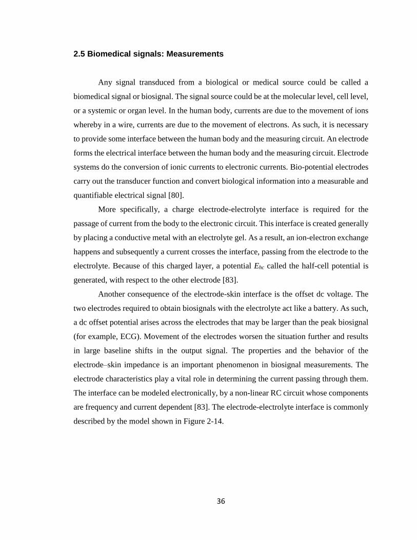
36
2.5 Biomedical signals: Measurements
Any signal transduced from a biological or medical source could be called a
biomedical signal or biosignal. The signal source could be at the molecular level, cell level,
or a systemic or organ level. In the human body, currents are due to the movement of ions
whereby in a wire, currents are due to the movement of electrons. As such, it is necessary
to provide some interface between the human body and the measuring circuit. An electrode
forms the electrical interface between the human body and the measuring circuit. Electrode
systems do the conversion of ionic currents to electronic currents. Bio-potential electrodes
carry out the transducer function and convert biological information into a measurable and
quantifiable electrical signal [80].
More specifically, a charge electrode-electrolyte interface is required for the
passage of current from the body to the electronic circuit. This interface is created generally
by placing a conductive metal with an electrolyte gel. As a result, an ion-electron exchange
happens and subsequently a current crosses the interface, passing from the electrode to the
electrolyte. Because of this charged layer, a potential Ehc called the half-cell potential is
generated, with respect to the other electrode [83].
Another consequence of the electrode-skin interface is the offset dc voltage. The
two electrodes required to obtain biosignals with the electrolyte act like a battery. As such,
a dc offset potential arises across the electrodes that may be larger than the peak biosignal
(for example, ECG). Movement of the electrodes worsen the situation further and results
in large baseline shifts in the output signal. The properties and the behavior of the
electrode–skin impedance is an important phenomenon in biosignal measurements. The
electrode characteristics play a vital role in determining the current passing through them.
The interface can be modeled electronically, by a non-linear RC circuit whose components
are frequency and current dependent [83]. The electrode-electrolyte interface is commonly
described by the model shown in Figure 2-14.

37
Figure 2-14: Electrical model of the electrode-electrolyte interface from [84]
Where Ehc is the half-cell potential, Rp and Cp represent, the impedance associated with
the electrode-electrolyte interface and Rs is the resistance due to interface effects. At high
frequencies, the impedance is Rs and at low frequencies, the impedance is Rs + Rp. At
middle frequencies, the electrode impedance is frequency dependent as illustrated in Figure
2-15.
Figure 2-15: Electrode impedance variation with frequency from [83]

38
Motion artifact poses challenges while measuring biosignals. The movement of the
electrode with respect to the electrolyte causes a momentary change of the Ehc (half-cell
potential) and a potential difference appears between the two electrodes during this
movement. This momentary potential is known as motion artifact and can be a serious
problem of interference in the measurement of bio-potentials, as illustrated in Figure 2-16.
According to the figure, the ECG signal within the green circle is affected by motion
artifact. A major component of this noise is at low frequencies and most difficult type of
noise to cancel, in particular, when the spectrum of motion artifact completely overlaps
with the desired signal.
Figure 2-16: The effect of motion artifact in ECG signal from [85]
In addition to the noises mentioned above, there are other external noise sources in
bio-potential measurements, as in Figure 2-17. Coupling capacitances between the power
line and lead wires cause parasite currents to flow through skin-electrode impedances. The
high-frequency signals from radio frequency (RF) sources and the signal components from
electric power lines are among them. The undesired noises add up with the desired signal
and appear at the input of the bio-potential amplifier. These cause displacement currents to
flow through electrodes and create a differential voltage between the impedances of the
electrode-skin interface [86].

39
Figure 2-17: Coupling capacitances, lead wires, and parasite currents from [87].
2.5.1 Biosignals: Processing
Biosignals are observations of physiological activities of organisms, ranging from
gene and protein sequences to neural and cardiac rhythms, to tissue and organ images [88].
Biosignal processing aims at extracting significant information from biosignals. With the
aid of biosignal processing, biologists can discover new biology, physicians can monitor
distinct illnesses, and engineers can develop medical instrumentation.
Decades ago, the primary focus of biosignal processing was on filtering signals to
remove noise [89, 90]. Sources of noise arise from the imprecision of instruments to
interference of power lines as mentioned before. Other sources are due to the biological
systems themselves under study. Organisms are complex systems whose subsystems
interact, so the measured signals of a biological subsystem usually contain the signals of
other subsystems. Removing unwanted signal components can then underlie subsequent
biomedicine discoveries. A fundamental method for noise cancelation analyzes the signal
spectra and suppresses undesired frequency components. Another analysis framework
derives from statistical signal processing. This framework treats the data as random signals;
the processing, e.g. Wiener filtering [91] or Kalman filtering [92], [93], utilizes statistical
characterizations of the signals to extract desired signal components. While these denoising

40
techniques are well established, the field of biosignal processing continues to expand,
thanks to the development of various novel signal-processing techniques, and supporting
technologies. The advancement of medical imaging modalities and signal processing
techniques (segmentation, motion tracking, sequence analysis, and statistical processing)
contribute significantly to the advancement of biosignal processing and analyzing.
2.6. Biomedical System: Architecture
Biomedical signals are primarily acquired and analyzed for detecting specific
physiological states to diagnose and evaluate therapy. The process of acquiring and
evaluating is done by a biomedical system [24]. The goal of such a system is to acquire
biosignal and process the same. A biomedical system, in general, consists of sensors,
electronic interface and computation block as shown in Figure 2-18. In Figure 2-18, the
computation unit is the brain of any medical instrumentation. It provides a primary user
interface and primary control for the overall system. It provides primary signal processing
functionalities for the system too. The computation unit is determined based on the specific
needs and is implemented through Microprocessor/Microcontroller [94], Digital Signal
Processor (DSP), Field Programmable Gate Array (FPGA) [95], or by a System on a Chip
(SoC) [50]. It is also equipped with a communication interface such as General Packet
Radio Service (GPRS) [86], Global System for Mobile Communications (GSM), Bluetooth
[96], or ZigBee [97] for data mobility.

41
Figure 2-18: Biomedical Instrumentation System Architecture from [98].
Biomedical measurement systems are defined to measure and usually record one or
more biosignals. The term biomedical measurement is quite general and includes image
acquisition and the acquisition of different types of diagnostic information. Information
from the biological process of interest must be converted into an electric signal via the
sensing element (transducer) as shown in Figure 2-19. Some analog signal processing is
usually required often including amplification and filtering (low pass or band pass). Since
most signal processing is easier to implement in the digital domain [99], the analog signal
is converted into a digital format, using analog to digital converter (ADC).
Figure 2-19: Architecture and Signal flow of an Instrumentation System from [83].

42
Once converted, the signal is often stored or buffered in the memory to facilitate
subsequent signal processing. Alternately, a in real-time application, the incoming data are
processed on the fly, often with minimum buffering, and may not be permanently stored.
In either case, digital signal processing algorithms can then be applied to the digitized
signal. These signal-processing techniques can take on a wide variety of forms with varying
levels of sophistication and they make up the major signal processing blocks in the
application. In some applications, such as diagnosis, a classification algorithm may be
applied to the processed data to determine the state of disease. Finally, some sort of output
is necessary for any useful system. This usually takes the form of a display, as in the
imaging system. There could be other auxiliary elements available in the medical
instrumentation for calibration, control and feedback, and transmission as shown in Figure
2.19.
Biomedical instruments can be classified in various ways. A system is called direct
when it measures a physiologic parameter directly, such as blood flow in the artery. It is
called indirect, when it measures a parameter related to the physiologic parameter of
interest (e.g., EKG recording). Direct electrical reading of the action potential in nerve
fibers using an implantable electrode system is an example of invasive medical
instrumentation [87]. An imaging system measuring blood flow dynamics in an artery, on
the other hand, is an example of a non-invasive medical system. Medical instrumentation
can also be classified as contact/remote. For example, an electrode must be connected to
the body of the subject for ECG recording, while an ultrasound imaging system can
measure internal deformations and forces without contacting tissue. Depending on the
objective of the measurement, the measurand can be sampled (e.g., temperature)
occasionally, or it could be sampled in a continuous way, such as ECG. The
instrumentation can work in analog mode [100], which is continuous in time and
continuous in amplitude. Medical instrumentation can also work in digital mode, whereby,
it is discrete in time and take only a finite number of sample values. Medical
instrumentation can also work in real-time mode (short processing time) or in delayed-time
mode (long processing time).

43
In designing and developing medical instrumentation, the researchers have
focussed their interest either in developing computing models, or designing systems to
implement known models or in both. In developing computing models, the researchers are
in search of alternative methods to estimate health indices, such as PTT-based BP
measurements. For the model establishment, researchers are using stored data from the
database and off-the-shelf hardware. While the others are proposing a medical
instrumentation system for biosignal acquisition, processing, and estimation of health
indices. A short survey of those models and systems will be presented in the following
section.
2.7 Biosignal Computing Platform: A survey
Engineers and researchers alike have been working in the field of bioengineering
intending to develop a mathematical model or formulae to compute various health indices,
such as BP measurement using pulse wave velocity and pulse transit time. As far as
instrumentation is concerned, various system architectures and implementations are being
proposed. There are medical instrumentation systems capable of monitoring a single
biosignal, like only ECG [101]. For example, an ECG monitor with 3, 5 or 12 leads.
Systems monitoring multiple biosignals, such as ECG, PPG, and others [102]. Another
trend among the researchers is to develop health instruments capable of not only
monitoring the physiological signals but also computing various health indices, such as BP,
heart rate, etc. [103], using various computing models.
The researchers also adopted various development platforms to realize the system.
Some systems are based on Microprocessor/Microcontroller, and some are implemented
on a Field Programmable Gate Array (FPGA) [104, 105]. Few of them are also realized
using System on a Chip (SOC) [106, 107]. In terms of data sharing, some systems are
stand-alone for in house use only. The others are capable of data sharing using body sensor
networks and wireless technology. For radio interface, GSM, Bluetooth, and ZigBee are
the common choices.

44
Whatever be the format used to develop the medical instrumentation system, these
are all about collecting physiological signals, such as ECG, PPG, etc., from the human
body and analyzing those biosignals, which are very small in amplitude with poor signal
to noise ratios. In the case of model establishment, the researchers use sample biosignals
from a data bank for proof of concept. To see the present state of the art in terms of systems
and models being developed and proposed by other researchers, it is now appropriate to
review some of the works.
In [108], the authors proposed a wireless health monitoring prototype system
specifically measuring the electrical activity of the heart. The proposed system was
developed with special consideration to make the device compact, portable, and with
minimum power consumption. The system was developed on a Microcontroller platform
along with discrete sensors and radio. In the case of a critical situation, the sensor is capable
of sending critical data to the network through wireless technology.
The authors in [109], proposed wireless, ambulatory, real-time, and auto alarm
intelligent telecardiology system. The system was developed surrounding an expert system
implemented on a Microcontroller platform equipped with a discrete analog front end for
signal acquisition and conditioning. The data acquisition unit transmits the acquired ECG
signal to the expert system (an application running on a portable device) using Bluetooth.
If an abnormal ECG is detected, the expert system sends an alert signal to the server situated
at the hospital.
Arrhythmia refers to a condition whereby the heartbeat shows an abnormal
sequence of electrical impulses. To detect arrhythmias, the authors in [110], developed a
cardiac function monitoring system. The developed system is based on multiprocessors.
The detection of arrhythmias is implemented in the embedded application. The developed
system comprises two parts, namely, the main module and the Bluetooth module. It also
houses a power management module. The acquisition and conditioning of the ECG signal
are through the discrete analog circuit. The processors (Master and Slave) communicate
with each other through a serial peripheral interface (SPI).
The authors in [111] proposed a Microcontroller based continuous non-invasive
cuff-less BP measurement system with an alarm mechanism. The proposed system is a
sensor network consists of BP and temperature sensors. Multiple process blocks were

45
implemented in the proposed system using analog discrete components. The system is
capable of monitoring multi parameters like BP, heart rate, and body temperature. If any
of the parameters exceed the threshold value, the proposed system can notify that using an
alarm circuit.
The work in [112] developed a remote doctor for homecare and medical diagnoses
on the cardiac patient. The system is capable of adapting itself to the patient. As such, the
system produces a personalized diagnosis based on the patient’s data and clinical history.
The developed system can be adapted to any type of patient. For that, a removable and
updatable memory is used to store clinical and personal patient data. Besides, internal read-
only memory stores information on the metrological status of the measurement system.
The system is based on an ECG sensor, implemented through analog discrete components.
A dsPIC is used as the core processor and a pocket PC for the analysis of the acquired
signal.
In [113], the authors developed an intelligent home health care embedded system
that can provide a health diagnosis at home. The architecture of the system allows
pluggable transducers for patients with different illnesses. As such, the transducers work
in stand-alone mode and exchange data with the expert system in a wireless sensor network
using ZigBee. Relevant parameters are extracted from the transducers using extensive use
of wavelet transforms.
Conventional BP devices are predominantly cuff-based and oscillometric. The
authors in [114] proposed a cuff-less BP system based on PTT delay. The wearable BP
device works with a smartphone. The PPG and ECG sensors are wirelessly connected to
the smartphone. The wearable BP device is divided into several process blocks and needs
an extensive synchronous mechanism. The blocks are implemented using discrete analog
components. A 4-LED PPG sensor is used to reduce power consumption.
In [115], the authors developed an ambulatory BP monitoring system, which is
cuff-less and based on PTT. According to the authors, the estimated systolic BP is within
4.8 ± 4.3 mmHg on healthy young subjects during sleep time. The developed system is a
strap-based wearable monitoring device for ambulatory ECG and PPG measurements. The
motion artifacts in the signal acquisition were handled manually.

46
The authors in [116] proposed a medical instrumentation system based on the
Arduino board for heart rate and temperature measurement. The system used discrete
sensor elements and the processed data were sent to a nearby server using a ZigBee
network. At the server, the medical data is further analyzed and if warrant alert signal is
sent to the caregiver using GSM network.
In [117], the authors developed a low-cost personal healthcare device capable of
recording ECG, Phonocardiogram (PCG), and body surface temperature simultaneously. It
is a stand-alone system implemented on discrete analog components to realize the basic
building blocks. The acquired signals end up into a laptop through a data acquisition system
for further analysis and monitoring. In this study [118], a non-invasive cuff-less PTT based
BP monitor was developed. The analog front end of the system is implemented using
discrete components including successive approximation register (SAR) based ADC of 12-
bit precision in a Microcontroller platform. According to the authors, they found a strong
correlation between measured PTT and SBP and a rather weak correlation between PTT
and DBP.
The paper [119] presented a BP estimation model based on PTT and pulse arrival
time (PAT) to estimate systolic BP (SBP) and diastolic BP (DBP). The developers also
designed data acquisition hardware for a high-resolution sampling of phonocardiogram
(PCG), PPG, and ECG. The system includes a data acquisition board, a portable computer,
and a commercial BP monitor. It also includes a force-sensing resistor (FSR) to measure
the instantaneous cuff pressure. The board and the computer communicates through a
universal serial bus (USB). The acquisition board is realized on an ARM processor using
four separate ADC channels. It also reports that the correlation coefficients for SBP and
DBP estimations are 0.89 and 0.84 respectively.
To improve people’s incentive for measuring BP, the authors in [120] developed a
wristband prototype for PTT-based BP measurement using multivariate regression
analysis. The proposed system consists of four layers, such as hardware, firmware,
smartphone app, and application layer. The developers used a Microprocessor as the
platform equipped with a built-in Bluetooth interface. According to the authors, the result
shows that in the normal BP range, the error in systolic BP is 6.9 ± 8 mmHg.

47
The authors in [121] developed a cuff based BP monitor. The developers used
Bluetooth technology to display BP values on an android-based smartphone. The system
consists of a management unit, power supply, and android-based mobile phone. The design
also includes a cuff and an air pump. The management unit sends the calculated BP value
to the mobile device through the Bluetooth interface. The paper also reports that the mean
and standard deviation of differences in readings is less than 5 and 8 mmHg respectively
in comparison to mercury sphygmomanometer.
The authors in [122] developed a new architecture for PTT estimation at the central
arteries using electrical bioimpedance, electrocardiogram, and continuous-wave radar. And
was used for cuff-less BP measurement. The proposed method obtains PTT and PAT from
the carotid and subclavian arteries and the sternum using four electrodes at the shoulder
and radar antennas on the sternum. The platform consists of several sub-systems, such as
a radar system, radio frequency (RF) transceiver, bioimpedance, and ECG readout circuits.
It concludes that moderate to strong correlation exists between PAT and SBP in all subjects
while moderate to strong correlation exists between PTT and SBP in specific subjects.
Arterial BP oscillates mainly at high frequency (HF) because of respiratory activity,
and at low frequency (LF) because of vasomotor tone. All previous studies show that PTT
can track BP variation in HF range, but is inadequate to follow the LF variation. The
authors in [123] presented a new indicator, the photo-plethysmogram intensity ratio (PIR),
which changes due to changes in arterial diameter, and, thus traces the LF variation of BP.
The developed algorithm is based on both PTT and PIR. The proposed model finds that
PIR can indicate the LF variation of BP, whereas PTT reflects the HF fluctuations of BP.
The results show that the mean ± standard deviation (SD) for the estimated systolic,
diastolic, and mean BP with the proposed model against reference are within acceptable
range with some limitations as acknowledged by the authors.
The authors in [124] designed a wireless biosignal acquisition system, which
integrates monitoring of ECG, EEG, and EMG. It also includes a wireless interface to
facilitate graphical representation on a computer screen. The proposed design was
implemented on an Arduino Uno board along with a Bluetooth device.
Health care monitoring through smartphones has been increasing, due to its
ubiquity, accessibility, and easy to use. Smartphones not only used for communication only

48
but finds its way in various aspects of human life. Several smartphone-based medical
devices are coming into existence. The paper [125] designed a wireless health monitoring
system using mobile phone accessories. The proposed system measures real-time ECG
with dry electrodes placed on the smartphone case. The acquired signal is stored and
analyzed in real-time through a smartphone application. The hardware system consists of
a discrete analog front end, a single chip Microcontroller (RFduino) embedded with
Bluetooth low energy module. The AFE is piggybacked on the RFduino.
The authors in [126] proposed an image-based BP measurement algorithm using k-
nearest neighbor and transfer learning results from Multiparameter Intelligent Monitoring
Intensive Care II (MIMICII) database to the real task. The study also introduced new PTT
features, which are specifically suitable for image-based PPG and domain adaption. The
study reports that the root mean square error of SBP reduced to 14.02 from 15.08. The
paper [127] proposed a robust low-cost eHealth Remote Health Monitor (RHM) system
intended to help facilitate the monitoring of patient’s physical health while they are at
home, driving, or relocated due to catastrophic emergencies. The proposed logical
architecture of the system consists of a frontend mobile app supported by a backend cloud
server, datacenter, and physical storage unit (local data center). The frontend app interacts
with Bluetooth enabled sensors to record patient’s health parameters along with physical
exercise data. The collected data is analyzed by the app and sent via data carrier service to
a server in a cloud or a private data center via a virtual private network (VPN).
The authors in [128] developed a multi-parameter smart armband that can record
pulse, temperature, and triaxial accelerations continuously. The armband was put to run for
38 hours and was able to record data. The hardware of the armband consists of main four
blocks. They are the sensors, the storage card, the Microcontroller, and the power
management block. The sensors include a reflectance pulse wave (RPW) sensor, an
infrared temperature sensor, and a triaxial motion sensor. The correlation coefficients for
heart rate and motion intensity index are in the range of 0.59 to 0.72.
The paper [129] developed a wearable health monitor that is based on continuous-
wave Doppler radar technology. The radar architecture is bistatic with a self-injection-
locked oscillator (SILO) tag and an injection-locked oscillator (ILO) based frequency
demodulator. The prototype operates in the medical and scientific bands. The SILO tag is

49
attached to the subject’s chest. It transforms the movement of the chest due to
cardiopulmonary activity and body exercise into a transmitted frequency-modulated wave.
The ILO based frequency demodulator, located 30 cm from the subject, receives and
processes this wave to yield the waveform that is associated with the movement of the
chest.
The design of wireless biosensors is essential to the realization of wireless health
monitoring. In that respect, microfluidic biosensors can play a vital rule. The paper [130]
designed a wireless all-analog biosensor for the concurrent microfluidic and physiological
signal monitoring. The sensor is composed of microfluidic sensing, physiological sensing,
all-analog signal compression, and wireless transmission circuits. The main feature is an
all-analog circuit capable of compressing two analog sources into one analog signal by the
analog joint source-channel coding (AJSCC). The detected physiological and biomarker
analog signal is directly compressed in the analog domain by an analog circuit and is
modulated and transmitted via analog radio frequency communication chain thus saving
power.
The authors in [131] presented a novel method of heart-rate calculation based on
the ECG signal acquired from the abdomen. In the center of the design, a belt, collects and
processes the signals and send health information to the smartphone via Bluetooth. The
belt connects to the core board through a flexible printed circuit. The core board also
contains an accelerometer to account for belly vibration. Overall, the system consists of
flexible printed ECG electrodes array, switch matrix, analog front end, accelerometer, and
a Bluetooth low energy SOC. The app in the smartphone displays the ECG signal along
with heart rate.
The paper [132] developed a portable health monitoring system. Sensors with a
communication protocol and reasonable user interface are embedded in the system for data
acquisition, computation, transmission, and display. In the center, BeagleBone Black is the
controlling hardware where sensors are connected to the general-purpose input/output
(GPIO) using standard jumpers. The GPIO pins are configured for functionalities like I2C
and SPI communication. The sensors are mounted on a separate custom design PCB.
Predefined feature values are used in algorithm and decision-making.

50
To shape the concept of connected homes, the authors in [133] proposed a health
monitoring system able to ensure a continuity of care between the home and the hospital
in spite of sensors heterogeneity. The authors developed a proof of concept showing the
possibility of medical data sharing using standard and proprietary protocols. The developed
android application was able to retrieve data from sensors implementing both standard and
proprietary protocols. These data can then be transmitted to the family doctor using
message queue telemetry transport (MQTT) protocol or to the hospital electronic
healthcare record (HER) through health level seven (HL7) protocol.
The authors in [134] developed a system to monitor the vital signs such as
temperature, BP, heart rate, gas sensor, and fall detection for elderly people at home. The
monitored values can be sent through mobile phones to concerned members. The proposed
system is developed surrounding an Arduino Uno board interfaced with required sensors.
The proposed system is simulated in Proteus. The paper [135] presented an outdoor
monitoring system for elderly people, which can transmit information on physiological
signals and falling events to a healthcare center at any time and from any place. To detect
the occurrence of any falling event, as well as the relative electrocardiogram signal of the
user, a multi-thread method is proposed. In the center of the system, a healthcare box,
which houses ECG acquisition circuitry, a GPS module, an RF front-end module with low
power ZigBee system, and a baseband module with 32-bit Microprocessor. An FPGA
platform is adopted in the baseband to execute the functionality of healthcare monitoring.
The measured results reveal that the accuracy of fall detection is between 63.44% and
80.77% and the corresponding accuracy for standing detection is between 15.14% and
91.67%.
The authors in [136] proposed a real-time health monitoring and alarming system
for patients. The proposed system has an embedded Microcontroller connected to a set of
medical sensors (related to the patient’s requirement) and a Bluetooth interface. Each
patient is considered as a node in a wireless sensor network and connected to a central node
at the medical center. Real-time signals from medical sensors are sent to the mobile phone
via Bluetooth connection. Then it is redirected to the central node via 3G/4G connection.
All the sensors at the embedded system implemented through discrete analog components.

51
The authors in [137] developed a remote health monitoring system based on
microelectromechanical system (MEMS) sensors to monitor movement and fall detection
for the elderly. Using MEMS sensors, Bluetooth, and GPRS remote communication
technology, whereabouts of the elderly’s fall and posture can be obtained on a real-time
basis.
In elderly people, heart attacks are associated with symptoms like body temperature
fluctuations, high BP, profuse sweating, improper cardiac rhythm, etc. The paper [138]
proposed a solution to integrate robust sensors capable of sensing and monitoring these
symptoms. The proposed system consists of sensors like pulse, body temperature, and
sweat sensor. A GSM module does the communication. The system consists of multiple
building blocks including two controller units. An RF module was used to transmit and
receive radio signals between two devices.
The authors in [139] investigated a cuffless nonintrusive approach to estimate PTT-
based BP. In this paper, three types of secondary peak detection methods are proposed to
reveal the secondary peak from the original PPG signal. Stored ECG, PPG, and BP
measurement data are used from the data bank, MIMICII. The paper reports that the
proposed detection mechanism improved the correlation relationship between BP and PTT.
The paper [140] stated a methodology to measure BP from the PPG signal. The
PPG signal was acquired through a PPG sensor connected to a personal computer and
filtered. Morphological features related to BP are extracted and analyzed through
LabVIEW and MATLAB. Random forest algorithm was used for predicting BP value. The
paper reports that compared to linear and multiple regression techniques random forest
showed better results. The percentage of error between measured and estimated values lies
from 6.71 to 13.2.
The authors in [141] proposed a novel continuous BP estimation approach that
combines data mining techniques with a traditional mechanism-driven model. In contrast
to mechanism-driven models based on the fixed hypothesis of the PTT-BP relationship for
different subjects, the proposed personalized BP model is based on individual patterns
derived from data mining. The proposed method extracts more BP indicators from
simultaneous ECG and PPG signals for each subject and determines the relative importance
for each subject by using a genetic algorithm-based feature selection model. The paper

52
reports excellent accuracy in static BP estimation, with a correlation coefficient of 0.852
for systolic BP, and 0.790 for diastolic BP, thus providing potentially novel insights for
cuffless BP estimation.
The authors in [142] proposed three key points to improve the accuracy of SBP
measurement. They are application of band-pass filter and wavelet de-noising to remove
noise on ECG data, introduction of a new characteristic point on ECG signal instead of R-
peak point, and heart rate are used to estimate pre-ejection period (PEP). As such, PTT is
equal to pulse arrival time (PAT) minus PEP. In the paper, twenty records were used from
the MIMIC database and the method was tested. The simulation result shows that mean
absolute difference (MAD), introduced by the IEEE standard, of SBP measurement,
decreased about 0.45 mmHg and the accuracy improved by an average of about 8.4%.
Monitoring personal health indices under the purview of a wearable body sensor
network (WBSN) is getting attention recently. The authors in [143] proposed a body sensor
network (BSN) system to estimate PTT-based BP. The BSN consists of three parts:
wristband, HR belt, and a smartphone. The wristband is worn as a wrist accessory to collect
PPG signals, and the HR belt is worn at the chest to collect ECG signals. The wristband
and the HR belt communicate with the smartphone via Bluetooth. Using a similar platform
(WBSN), the authors in [144] presented a wearable IEEE 802.15.4-based WBSN for
estimating the BP continuously and non-invasively. The sensor network (WBSN)
composed of photoplethysmographic sensor node located on the forehead, and an
electrocardiographic sensor node located on the chest, were used to measure the
propagation time of the pressure wave from the chest to the forehead. The authors in [145]
developed a wireless BP monitoring system, which provides a useful tool for users to
measure, and manage their daily BP values. The system includes an ARM-based BP
monitor with a ZigBee module and a PC-based management unit with a database. The
wireless BP monitor measures BP, and heart rate. Then store and forward the measured
information to the management unit through the ZigBee interface.
Implementing medical instrumentation on a field-programmable gate array (FPGA)
is also getting momentum. The authors in [146] reported the design and implementation of
a standalone FPGA-based ECG monitoring device that can display the ECG signal along
with heart rate. The proposed hardware is based on Xilinx’s Spartan-3 FPGA. The system

53
also includes discrete components, such as an amplifier, filter, and ADC. The FPGA is the
central processor and programmed to realize ECG signal sampling and processing.
After going through the above literature survey, one can get a clear picture of the
present state of the art in the field of medical instrumentations, specifically BP
measurement in a non-invasive and continuous manner. According to the survey, the PTT-
based approach for cuff-less BP monitoring has captured the interest of many investigators.
The steps involved in this approach are the measurement of proximal and distal arterial
waveforms; estimation of PTT from the waveforms; and calibration of PTT to BP. In the
survey, for convenience, ECG was employed as the proximal and PPG was employed as a
distal waveform respectively. And PTT was estimated through peripheral arteries and the
arm in particular. It is also found that for feature detection, in general, Pan and Tompkins
signal processing method was used. Among the researchers, one group was involved in
developing models relating to BP and PTT. The models vary from linear to non-linear.
Some of the models include covariates in addition to PTT. The covariates include
cardiovascular variables such as heart rate and physical variables such as height. The
models were tested on systems made of off the shelf hardware or simulation tools using
stored biosignals from the data bank. While the other group used custom-built hardware
platforms and implemented a chosen model in it.
In the survey, most of the hardware implementations used discrete analog front ends
for data acquisition and conditioning. Thus vast of the signal processing was done in the
analog domain with limited flexibility and accuracy. Another noticeable trend in those
implementations is the usage of multiple boards and multiple processors. As such, the
sensors are spread around. That raises the possibility of a synchronization problem among
the measured waveforms. PTT based BP measurements need synchronization among the
measured pressure pulses. It also demands a constant calibration maneuver. It is noticed in
the survey that most of the implementations either ignore this maneuver or did little to
implement this important phenomenon.

54
2.8 The Evolution of Sensor Analog Front Ends
We are surrounded by the analog world and we need sensors to read and convert
the analog signals into digital data using analog-to-digital converters (ADCs). The sensor
output requires amplification and conditioning to provide the best possible signal to the
ADC. This combination of conditioning circuitry is called an analog front end (AFE). With
the advent of the integrated circuit (IC) Microprocessor and later the invention of the digital
signal processor (DSP) by Texas Instruments in 1978, the requirement to convert physical
effects to digital signals became a focus for engineers [147]. The analog front end, an
essential system building block to a sensor circuit, amplifies and filters sensor signals that
are often weak, or its electrical configurations differ from the one used by the system
controller. The AFE that performs this vital bridging function is often difficult to simulate
and must be adjusted because of specific component behavior, board layout, and nearby
noise sources.
The limited output signals from the sensors are usually conditioned using
operational and differential amplifiers that convert these tiny changes in the sensors to large
enough to fully utilize the dynamic range of the ADCs and helps maintain the signal-to-
noise ratio (SNR). Beyond the amplification and conditioning of the signal, filtering is
required to remove unwanted signals from the system. The ubiquitous 50 and 60 Hz power-
line noise can impart noise into a sensor system. This electric noise can add significant
error to a low-frequency signal from a sensor and must be filtered out. A major issue with
ADCs is aliasing caused by frequency components present in the signal that is greater than
the Nyquist Criterion (half the sampling frequency or Fs/2). To prevent this, an analog anti-
aliasing filter is placed before the ADC input. For most SAR (Successive Approximation
Register) based ADCs, this filter can be challenging and require several orders to provide
the correct cutoff.
Recent technological advancements have resulted in ADCs with a combination of
speeds, resolution, and power that were impossible before. To simplify the system design
and provide sensor flexibility, semiconductor vendors have begun to integrate all of this
front-end analog circuitry into a single device. For example, the ADS1293 is a fully
integrated analog front-end ideally suited for ECG signal conditioning and ECG

55
application. It is programmable via the SPI interface to configure every signal chain
parameter inside the AFE. Unprecedented developments in the semiconductor technology
changing the façade of sensor technology and emerging as Smart Analog [148]. The Smart
Analog technology implements a range of AFE topologies designed to be easily
programmed to support sensors with a single device. The technology uses a set of
configurable amplifier circuits, which can be tailored using intelligent and intuitive
software. Since field-programmable, the circuit characteristics can be modified for sensor
drift and can be easily tuned to meet the system requirements.
Technological advancements also made the user-programmable FPGAs (Field
Programmable Gate Array), a new frontier of instrumentation. One of the unique
characteristics of FPGAs is the ability to execute computationally intense and increasingly
parallel signal-processing algorithms in real-time [149]. As such, the total analog front end
and the system controller can be implemented on an FPGA with higher computational
performance. Thus, FPGAs - often augmented with graphical programming units (GPUs)
- have become a central element of advanced system design applications.
The world around us is analog, and converting physical phenomena to electronic
signals requires a multitude of sensor technology. Many of these sensors require a
significant amount of analog circuitry to operate properly. With the introduction of highly
integrated AFEs, entire sensor systems can be placed on a single device, such as pressure
sensors where the sensing element is part of the die. With the advances in micro-
electromechanical systems (MEMS), this integration even further providing everything on
a single device and find their way into our everyday lives. All of these will be possible due
to advances in microelectronics, sensor technology and the AFEs that make them work. By
solving these challenges, our industry is enabling engineers and researchers alike to use
instrumentation platforms in a much wider range of applications. For many engineers, the
ability to execute custom, advanced signal-processing algorithms on the AFEs of an
instrument eliminates the need for them to design additional hardware and paves the way
to design instrumentations with a new design paradigm.

56
Chapter 3 : Approach and Research Methodology
From the literature survey, it is clear that ubiquitous health monitoring is on the
horizon. Firstly, there is a profound need for continuous and non-invasive technologies,
which can be used in ambulatory settings for non‐invasive monitoring of health indices,
such as BP, for example. Secondly, it is feasible. There have been many relevant
technological developments in the recent past, such as in sensor technology,
miniaturization, pervasive computing, and smartphones [150]. Also, there is mounting
evidence that pulse transit time (PTT, i.e., the time delay for the pressure wave to travel
between two arterial sites) can be the basis for continuous, cuff-less BP measurement. As
far as a computing platform is concerned, and considering the latest evolution in analog
front ends, it is also clear that realizing a signal conditioning circuitry using programmable
highly integrated analog front-end controllers (AFEs) instead of discrete analog
components can bring significant improvements in signal processing. That way, the bulk
of the signal processing can then be done in the digital domain as opposed to the analog
domain. This transfer will enable one to implement a custom algorithm in the analog front
end. Since the AFEs are programmable, the circuit characteristics and signal parameters in
the signal path can be configured to meet system requirements. That way, one can execute
custom signal-processing algorithms in an AFE thus resulting in a hardware platform with
a smaller footprint. It is also evident that using the latest family of processors along with
programmable AFEs, one can improve overall system performance in terms of speed, size,
and power consumption.
Taking into account of all of these, this thesis proposes and develops a biosignal
computing platform, named TasDiag. TasDiag is a multi-modal embedded system, capable
of estimating blood pressure (BP), oxygen saturation level (SpO2), heart rate (HR), and
body temperature of human subjects. Following the overwhelming trend in the survey, this
thesis also implements PTT-based BP measurement for convenient cuff-less BP reading.
PTT-based BP measurement lies in the fact that the velocity at which pressure pulses
propagate along the arterial tree depends on the underlying BP. Experimental results also
show that 1/PTT is linearly related to BP. As such, if we can measure PTT, that can be
mapped to the underlying BP through some regression process. PTT can be measured from
57
the relative timing between two feature points on the proximal and distal waveforms. In
this thesis, the ECG signal is employed as the proximal waveform and PPG is employed as
the distal waveform. For that, ECG and PPG signals were acquired from subjects and
processed to detect feature points on them and using the feature points, PTT was calculated.
Feature points are the characteristic points on the signals, such as maxima, minima on the
signals. Feature points along with other signal parameters, such as period, maximum, and
minimum amplitudes were also measured to calculate other heath indices (heart rate,
oxygen saturation level, etc.,). Besides, for design verification and performance
measurements, long-term recordings of various health data were collected from human
subjects using TasDiag and industry-standard instruments. The Data collection process was
guided by the research ethics board document (REB #14522). The collected data were then
subjected to various statistical analyses for verification and performance measurements and
will be shared in chapter four.
This thesis entails two core areas: They are background research on human
physiology, specifically, cardiovascular physiology, and design and development of an
embedded system for biosignal computing. Cardiovascular physiology is described in
chapter 2. Every embedded system has two integral parts. A purpose-built system
application and a hardware platform to house that application and facilitate its execution.
In this case, an application-specific to biosignal processing and computing with a
comprehensive recalibration scheme has been developed under the umbrella of a system
application running on the hardware platform. Biosignal processing is accomplished
through numerous custom algorithms, state machines, and computing techniques under the
purview of the system application. The hardware platform is designed using open
architecture, whereby, in the center, there is a system controller, which is surrounded by
biosignal specific highly integrated programmable AFEs. As such, the focus of this chapter
is to highlight the custom algorithms, computing techniques, and state machines used in
the system application. Also, the hardware architecture, and integration of the various sub-
systems used in the design are also described in this chapter.

58
3.1 Algorithms and Computing Techniques
TasDiag is designed to calculate various health indices of the subject from the
acquired biosignals. The calculated indices are blood pressure (BP), oxygen saturation
level (SpO2), heart rate (HR), body temperature. To calculate BP, SpO2, and HR, ECG and
PPG signals are acquired. Depending on the health index being calculated, these signals
can be acquired individually or parallelly. Acquired signals need conditioning, and
processing, as they are crisscrossed with various noises including motion artifacts. It is
necessary to detect feature points on the biosignals to calculate PTT. Feature points are the
characteristic points on the signal, such as maxima, minima, maximum slope, etc. It is also
important to determine signal parameters, such as period, amplitudes, etc. For that, the
AFEs are to be set at proper operating conditions and the acquired biosignals need to be
processed under program control. There are numerous function modules deployed to do so
as shown in the class structures in section 3.3.
The signal acquisition and processing starts with the acquisition of the biosignal
(ECG, PPG) from the subject and goes through the primary conditioning in the AFE under
program control. To be specific, the acquired signal goes through multi-stage amplification
and filtering. The gain, cut-off frequency, bandwidth, sampling rate, decimation rate, and
data output rate (ODR) are set under program control using set rules and algorithms. After
the primary conditioning, the acquired biosignal is sampled by the system controller from
the AFE and subjected to secondary conditioning for filtering and smoothing using custom
algorithms and techniques. The filtered sample then goes through further processing to
determine its slope, edge, and state in view of signal feature detection for PTT calculation.
In this thesis, the R wave on the ECG signal and the maxima point on the PPG signal are
considered as feature points. Through this process, other timings and amplitude parameters
of the biosignal under acquisition are also measured. The detected features are used to
calculate various health indices. The signal path and the processes followed by a sample
starting from acquisition to health index calculation is shown in Figure 3-1. This life cycle
of a signal sample is executed in a program loop and the figure shows the data flow
followed in the program loop.

59
According to Figure 3-1, a signal sample (either ECG or PPG) is collected through
the corresponding signal specific AFE under program control. The collected sample goes
through the primary conditioning process inside the AFE. The primary conditioning
process starts filtering the sample by an electromagnetic interference filter (EMI) to reduce
interference from other instrumentations followed by amplification by an instrumentation
amplifier. The amplification is required to cover the dynamic range of the analog to digital
converter (ADC) and help improve the signal to noise ratio (SNR). The amplified sample
is then subjected to a delta-sigma ADC and finally to a digital filter. This ends the primary
conditioning of the acquired sample. The sample then enters into the secondary
conditioning module, implemented in the system application. Here the signal sample passes
through a set of pulse filters so that a triangular pulse wave can be obtained at the output.
The triangular output enables the realization of the original waveform. The sample also
goes through a combination of low and high pass filters for dc removal and reduce the
effects of motion artifacts. The filtered sample is then subjected to a set of slope filters to
calculate its slope as shown in Figure 3-1. The slope information is used to determine the
state of the signal under the purview of a state machine. Once the state is determined, the
next step is to detect features (maxima, minima) points on the signal. The feature
information is used to calculate the signal period and PTT. During the life cycle of a signal
sample, various custom algorithms and techniques are used in acquisition, conditioning,
and processing the signal sample, which is described in the following sub-sections:

60
Figure 3-1: Life Cycle of a Signal Sample

61
3.1.1 Gain Calibration
AFE4400 from Texas Instrument is ideally suited as a front-end for PPG
(Photoplethysmography) application. This AFE is custom-built to acquire and condition a
photoplethysmography signal. The receiver section of the AFE consists of a differential
current-to-voltage (I-V) trans-impedance amplifier (TIA) that converts the input
photodiode current into an appropriate voltage. The feedback resistor of the amplifier (RF)
is programmable to support a wide range of photodiode currents. The RF resistor and the
feedback capacitor (CF) form a low-pass filter for the input signal current. As such, CF is
also programmable. These two components (RF and CF) determines the gains at stage 1 and
stage 2 in the signal path.
The output from these stages ends up at the input of the delta-sigma analog to
digital converter. It is important to present a tangible amount of signal voltage to the ADC
to utilize its full dynamic range. This in turn help compensate offset and improves the signal
to noise ratio (SNR). For that to happen, the AFE is dynamically calibrated through a
calibration routine, implemented in the system application. The flow chart shown in Figure
3-2 has been implemented painstakingly in the calibration routine.
The flowchart is quite complex, but in short, the DC-Value is set based on the
average of 16 readings and then compared with the target thresholds (both high and low).
If the set value is not within the target thresholds and if the RF value is not already at its
extreme low values, the RF value is adjusted and a new set of readings are taken with that
adjusted value.
To achieve the threshold level, another variable, ILED_CURR is also adjusted
starting with the minimum value (5 mA) to the highest possible value (45 mA). As such, it
is a two-prong adjustment process to set the operating voltage within the threshold level.
If necessary, stage 2 gain also comes into action. If the measured DC-value is less than
threshold low, the RF is set to 1 MΩ and the process is repeated. Once the DC-value falls
within the desired limit, the device is said to be in a ready state for normal data acquisition.

62
Figure 3-2: Flow chart for PPG calibration routine from [151]. Courtesy Texas Instruments.

63
3.1.2 Signal Slope Calculation
To calculate PTT and other signal parameters, such as frequency, period, and
amplitude, we need to identify some feature (characteristic) points on the signal and the
time instant of those characteristic points. To identify feature points on the waves (ECG
and PPG), it is important to analyze and follow the signals closely. The characteristic points
on the pulse wave generally used, are the maximum, the minimum, the average point
between the maximum and the minimum, the maximum of the first derivative, the
maximum of the second derivative of the pulse wave, the intersection of line tangent, and
the intersection of two line tangents. In this study, the maxima and minima of the wave are
used as the characteristic points.
To identify those characteristic points, it is needed to determine the edges (slopes)
of the pulse wave. Edges in images are areas with strong intensity contrasts – a jump in
intensity from one pixel to the next. Edge detecting of an image significantly reduces the
amount of data and filters out useless information, while preserving the important structural
properties in an image. There are many ways to perform edge detection. However, the
majority of different methods may be grouped into two categories, gradient, and laplacian.
The gradient method detects the edges by looking for the maximum and minimum in the
first derivative of the image [152]. The edge detection mechanism can also be based on the
Sobel edge detector principle, which is a discrete differentiation operation, computing an
approximation of the gradient of the image intensity function at each point in the image.
In this thesis, the edge detection mechanism is based on the Sobel edge detection
principle and is implemented through slope filters working under the purview of a state
machine. The algorithm used to calculate the slope (a unitless quantity used for edge
detection) of the signal is shown in Figure 3-3. The slope calculation is divided into two
sections, such as conditioning and calculation as shown in the figure. In the first part, the
sample goes through the process of filtering and the filtered sample goes through the
process of slope calculation in the second part. The raw biosignal is acquired, conditioned,
and digitized by the respective AFE under program control. Each signal sample is then
subjected to First Pass Filter, which is a moving average filter. The output of the First Pass
Filter goes as input to the Second Pass Filter, another moving average filter. This

64
arrangement gives a triangular impulse response, which is useful in signal processing as
more signals that are realistic can be derived. Both filters having 4 elements each. The
output of the Second Pass Filter goes through a combination of low pass and high pass
filter. The constant for high pass filter is programmable and is used to set the fc (cut-off
frequency). For example, for a constant (ᾳ) value of 64, and with a sampling frequency of
200 Hz, the fc is calculated as below:
𝑅𝐶 = ∆𝑇 1 −𝛼
𝛼 (3.1)
= 1
200
1 − 1
641
64
= 1
200 ×
63
64 ×
64
1
= 63
200 = 0.315 (3.2)
𝑓𝑐 = 1
2𝜋𝑅𝐶 =
1
2𝜋×0.315 = 0.5055 𝐻𝑧 (3.3)
The filtered sample is then subjected to another set of filters, known as slope filters.
The set is consists of two moving average filters with three elements each. The slope for a
specific sample is calculated by taking the difference between the average values of the
samples ahead and before the sample of interest. That is, the state machine will calculate
slope for sample S4, for example, while it has just acquired sample 7. To calculate the slope
for S4 (sample 4), the average value for S7, S6, and S5 will be calculated first. Then, the
average value for S3, S2, and S1 will also be calculated. Finally, the difference between
these two average values is the slope at S4, which is shown in equation 3.4.
Slope at S4 = (S7+S6+S5)/3 – (S3+S2+S1)/3 (3.4)
The signal in question is always changing its state in the time domain. At the time,
it can travel in a positive direction and at other times, it can travel in the negative direction
giving rise to the possibility of having both positive and negative slopes. This scenario is
shown in Figure 3-4.

65

66
Figure 3-3: Flow diagram for slope calculation at S4 (Sample# 4)
Slope Filter1
Sx In
Slope Filter2
S7 S6 S5
S4
S3 S2 S1
Slope at S4 = (S7+S6+S5)/3 – (S3+S2+S1)/3
AAA
End
(Filtered)

67
Figure 3-4: Slope calculation at S4 (Sample# 4) for both polarity of signal state
S7
S6
S5
S4
S3
S2
S1
S1
S2
S3
S4
S5
S6
S7
Slope at S4 = (S7+S6+S5)/3 – (S3+S2+S1)/3

68
3.1.3 Signal Slope Threshold Estimation
Characteristic points on the biosignal, such as maxima, minima, and slope are used
to calculate various timing parameters including PTT. Pulse transit time (PTT) is the time
difference between two characteristic points on the synchronized ECG and PPG signal
measured in the same cardiac cycle. To determine those feature points on the signal, it is
paramount to estimate the slope and amplitude of the signals in use. Biosignals differ from
subject to subject and differ for the same subject with respect to time of the day. It is a
dynamic phenomenon. As such, it is important to estimate the slope and amplitude of the
signal dynamically. For that, in this thesis, the signal slope is dynamically estimated
through a state machine. The threshold slopes are estimated at the beginning of sample
collection, one for positive slope (ThresholdUpper) and the other for negative slope
(ThresholdLower). During the sample collection process, the incoming sample’s slope is
compared against these threshold slopes to ascertain the signal’s state. The algorithm and
signal flow for the threshold estimation process are shown in Figure 3-5.
In short, the algorithm used for threshold slope estimation is as follows: Around
2048 samples (considering the available RAM in the system, and to accommodate
approximately 10-12 cardiac cycles) of the biosignal (ECG or PPG) are collected and the
slope of each sample is calculated using the algorithm mentioned in section 3.1.2. The
calculated slopes are stored in a buffer, SlopeArray. There are two types of slopes possible
as shown in Figure 3-4, positive and negative.
Once all the slopes (2048 in total) are calculated and stored, the algorithm starts
with searching the negative maximum (negaMax) slope value in the SlopeArray. Once
found, it goes for the corresponding positive maximum (posiMax) slope value. Because of
the biosignal characteristics (both ECG and PPG), the negative maximum and positive
maximum slopes occur in pairs per cardiac cycle. First the posiMax followed by negaMax.
The algorithm saves the just found negaMax value in an array (NegaSlopeValue) along
with its index (positional value, i.e., sample number). The posiMax value is also saved in
a separate array (PosiSlopeValue) and its index value.

69

70

71

72

73

74

75

76
Figure 3-5: Flow diagram for Signal’s Threshold slope estimation

77
The index of the just found posiMax and negaMax pair are taken as the reference
point (anchor point) for searching the other pairs in the SlopeArray. For that, a window of
200 slope values (covering one cardiac cycle) from this reference point is searched in the
forward direction, towards the end of SlopeArray. The next pair of negaMax and posiMax
is found and stored along with their index values in the corresponding arrays as mentioned
above. For verification, the algorithm checks the distance (in terms of time) between the
last found pair and the latest one. If the distance between the pairs lies between 425
milliseconds (equivalent to 85 samples) to 1000 milliseconds (equivalent 200 samples),
then the newly found pair is taken as a valid pair and is stored. It is worth to mention that
the samples are collected at 5 mS interval and the default R-R (for ECG) cycle duration is
600 mS to 1000 mS, considering 60 to 100 bit per minute (bpm). Besides, the distance
between the posiMax and negaMax within the same pair must be within 80 milliseconds
(equivalent to 16 samples) window; considering the QRS interval is 80 milliseconds [30].
The next window is set up from the last found pair position towards the end of the
SlopeArray and the next pair is searched, found and stored. This process continues until
the end of the SlopeArray in the forward direction. Once done, now, the search starts from
the anchor point in the reverse direction (towards the beginning of the SlopeArray). Again,
a window of 200 slopes is set up and the next pair of posiMax and negaMax slope values
are searched, found and stored. The process continues until all the slopes towards the
beginning of the SlopeArray are covered. The window view of the above process is shown
in Figure 3-6. This figure is an example case, whereby, from the reference point, there are
5 windows in the forward direction and 4 windows in the backward direction, altogether 9
windows, to be searched to cover all the 2048 slopes stored in the SlopeArray and
processed once to calculate ThresholdLower and ThresholdUpper slopes.
In short, the above process separated all the positive maximum slopes and the
negative maximum slopes occurred in each cardiac cycle. If there are 12 cardiac cycles in
those 2048 samples, for example, there are 12 positive maximum slopes are stored in the
PosiSlopeValue array and 12 negative maximum slopes are stored in the NegaSlopeValue
array out of the above process. The slope values are then arranged in ascending order. Also,
if there are any extreme outliers, they are discarded and the arrays are rearranged
accordingly. In the end, we have two arrays, one with all the positive maximum slopes and

78
the other with all the negative maximum slopes arranged in ascending order. To estimate
the threshold values the following empirical method is applied:
For estimating the threshold value for positive slopes (ThresholdUpper), first, the
average slope is calculated by averaging all the positive slopes in the array
(PosiSlopeValue). Then the lowest slope in the array is subtracted from the average value
and the result is divided by two.
Figure 3-6: Slope array and Search window structure. From the reference point, there are
5 windows in the forward and 4 windows in the backward direction, as an example case.

79
The just calculated value is then subtracted from the average value and that is the
ThresholdUpper value for positive slopes. The reason behind this mathematical maneuver
is to put the ThresholdUpper value towards the left of the average value. This way, less
steep positive slopes observed during those cardiac cycles can be accommodated. For
estimating the ThresholdLower value for negative slope, the highest negative slope in the
array (NegaSlopeValue) is incremented by an arbitrary number 100 and that sets the
ThresholdLower value for negative slope. Again, the reason behind this arbitrary addition
is to accommodate less steep negative slopes observed in those cardiac cycles. It was also
noted that most of the other negative slopes lie within 100 points from the highest negative
slope. For example, if the calculated negative maximum slope is -2000, adding 100 to it
will make the ThresholdLower value to -1900 and enables the algorithm not to discard
some less steep slopes in the signal. To verify this mathematical maneuver, sample data
from subjects were collected (Table A-1 and Table A-2) and signal peaks were detected as
described in section 3.1.6 using the threshold slopes calculated as above. Signal peaks were
detected at a success rate of a minimum of 70% to a maximum of 100%. The mathematical
model thus developed to calculate slope thresholds is shown in Figure 3-7. It can also be
modeled using the following mathematical equation as below:
ThresholdUpper = Average of the elements in PosiSlopeValue array (3.5)
ThresholdUpper = ThresholdUpper – (ThresholdUpper – lowest element in array)/2 (3.6)
ThresholdLower = Highest negaMax value in the array + 100 (3.7)

80
Figure 3-7: Mathematical model for Threshold Slope Calculation
Lowest +ve Slope
ThresholdUpper Average +ve
Slope
Highest +ve Slope
Mathematical Model: ThresholdUpper
Lowest -ve Slope
Highest –ve Slope
ThresholdLower
+100
Mathematical Model: ThresholdLower

81
3.1.4 Signal State Determination
Time-varying signals, like ECG and PPG, change their state with respect to time.
To detect characteristic points, such as maxima and minima on those biosignals, it is very
important to follow the signal very close to ascertain their state. A state machine with a
custom algorithm has been developed and applied to determine the state of the signal
concerning every sample collected. According to the algorithm, the signal passes through
five states. They are initial, falling, valley, rising, and peak. It is assumed that the biosignal
(ECG and PPG alike) goes through these states. These states are shown in Figure 3-8. The
state ‘initial’ does not represent any specific point on the signal rather it represents the
starting point of the detection process. However, the sequence is very important. The
detection process is based on an algorithm, and the flow diagram is shown in Figure 3-9.
Figure 3-8: Signal state definition
According to the flow diagram, the state machine starts with the INITIAL state,
which is the starting state. The INITIAL state does not represent any specific point on the
signal. It could be any point on the signal. It is the starting point for the state machine to
start with. Each sample is collected under program control and its slope (currentSlope) is
calculated using the algorithms mentioned before. This currentSlope is compared against
the ThresholdLower as shown in the flow chart. If the currentSlope is greater than the
4157000
4158000
4159000
4160000
4161000
4162000
4163000
0 200 400 600 800 1000 1200
AD
C V
alu
e
SampleNo
ECG
Initial Falling Rising Peak
Valley

82
ThresholdLower, the signal remains at INITIAL state and Maxima and Minima variables
are updated. These are the two variables to hold the maximum and minimum amplitudes
of the signal. The signal remains at INITIAL state as long as the currentSlope remains
greater than the ThresholdLower value. Once the currentSlope of the next sample becomes
lower than the ThresholdLower, the signal enters into the next state, which is the FALLING
state.
Once in FALLING state, the next sample is collected and its slope (currentSlope)
is calculated. If the previousSlope is less than zero and the currentSlope is greater than zero
(i.e., there is a transition from negative-going to positive-going) then signal enters into the
VALLEY state. If not, it remains in its present state (FALLING state) and the process of
collecting the next sample, calculating its slope, and comparison is repeated. The Maxima
and Minima variables of the signal are updated based on its present state.
If there is a transition in slopes, the signal enters into the VALLEY state. When in
the VALLEY state, the currentSlope is compared with the ThresholdUpper slope value. If
currentSlope is greater than ThresholdUpper, the signal enters into the RISING state.
Otherwise, it falls back to FALLING state to bypass false valley on the signal. Besides, to
avoid the false transition to the RISING state, the algorithm forces the state machine to
remain at the valley state for some time by bypassing some of the samples (calculated
through observations). The Minima variable is updated while at the VALLEY state. The
Minima value at this state represents the signal’s lowest value (Negative Peak).
At RISING state, like before, the next sample is collected and its slope is calculated.
If the previousSlope is greater than zero and the currentSlope is less than zero, i.e., there is
a transition in slope from positive-going to negative-going, the signal enters into the PEAK
state and represents the end of one cycle of the signal. If not, the signal remains in its
present state that is RISING state.
At the PEAK state, it is assumed that the state machine has just completed the cycle
of state transition and the signal has reached its maximum peak. The Maxima variable is
updated at the PEAK state. The Maxima value at this state represents the signal’s highest
value (Positive Peak).

83

84

85

86

87
Figure 3-9: Flow diagram for Signal State determination
The state machine starts the next cycle of operation by putting itself at the INITIAL
state, the starting state. Figure 3-10 shows the state diagram of the algorithm described
above. According to the diagram, the state transition is based on a change in signal slope.
The state machine starts from the INITIAL state and ends at PEAK state.

88
Figure 3-10: Signal State Transition diagram. SC: Slope Current, SP: Slope Previous, TL:
ThresholdLower, TU: Threshold Upper.
Once started from the INITIAL state, it remains in this state as long as the current slope of
the signal remains higher than the ThresholdLower value. Once the slope of the signal
becomes lower than the ThresholdLower value, it enters into FALLING state. In this state,
the current slope of the signal must be greater than zero and the previous slope of the signal
must be less than zero to transit to VALLEY state. Once at VALLEY state, the current
slope must be greater than ThresholdUpper to transit to RISING state. If not, the state
FALLING
VALLEY
INITIAL
RISING
PEAK
Signal State Transition
TL> SC
TL < SC
0 > SP && 0 <= SC TL > SC
0 < SP && 0 >= SC
TU < SC
0 < SP && 0 >!= SC
0 > SP && 0 <!= SC

89
machine falls back to FALLING state. When the state machine reaches the RISING state,
the current slope of the signal must be less than zero and the previous slope must be greater
than zero to transit to PEAK state. This transition indicates that the signal has reached its
peak and completed its cycle.
3.1.5 Signal Feature (Maxima/ Minima) Calculation
The estimation of health indices largely depends on characteristic points on the
biosignal in question. The proposed biosignal computing platform also uses characteristic
points for the calculation of health parameters. Specifically, peak detection is one of the
important features used in the proposed design. Detecting the signal peak is paramount to
the accurate estimation of various health indices. The algorithm used in detecting the peak
of the signal is shown in Figure 3-11.
Two macros (SignalMin and SignalMax) are declared and defined as a preprocessor
directive in the system application. They are used extensively in the algorithm to calculate
the minimum and maximum of two numbers respectively. Two variables, Minima and
Maxima are also declared to hold the updated amplitude of the sample, one for the lowest
amplitude and the other for the highest amplitude of the signal. The algorithm works under
the purview of the state machine described in the previous sections. As shown in the flow
chart, the sample is collected under program control and depending on the state of the
signal; the Maxima and Minima variables are updated with the just collected sample
amplitude.
The next sample is collected and if the signal is in its INITIAL state (determined
through state machine), the Minima is updated with the sample amplitude. This process is
repeated as long as the signal remains at this INITIAL state. When the signal enters into
the FALLING state, the minimum of the present Minima and next sample’s amplitude is
calculated through the SignalMin macro. And the Minima variable is updated with this new

90
minimum. This updating process is repeated as long as the signal remains at FALLING
state.
When the signal is in VALLEY state, the Minima variable is updated with the
minimum of the current Minima and the next sample’s amplitude through the usage of
SignalMin macro. The Maxima variable is also updated with the maximum of the current
maxima and the next sample’s amplitude through the usage of SignalMax macro. This
process is repeated while the signal remains at VALLEY state. The value in Minima, at
VALLEY state, represents the lowest value of the signal (Negative Peak).
Once the signal comes out of VALLEY state and enters into the RISING state, the
maximum of the current Maxima and next sample’s amplitude is calculated through the
SignalMax macro and the Maxima variable is updated with the new maximum. This goes
on as long as the signal remains at RISING state. Once in PEAK state, the value in the
Maxima variable represents the signal’s highest value. At this point, Maxima represents
the positive peak and Minima represent the negative peak of the signal in acquisition.

91
Start
#define SignalMin (a, b) (a > b? b: a)
#define SignalMax (a, b) (a <b? b: a)
Data = NextSample
State ==
INITIAL?
Minima = Data
YES
AAA
AAA
State ==
FALLING?
Minima = SignalMin
(Minima, Data)
AAA
YES
BBB
NO
NO

92
Figure 3-11: Flow diagram for Signal feature extraction
BBB
State ==
VALLEY?
Minima = SignalMin (Minima, Data)
Maxima = Data
YES
AAA
State ==
RISING?
Maxima = SignalMax (Maxima, Data)
State ==
PEAK?
AAA
YES
Maxima = SignalMax (Maxima, Data)
YES
AAA AAA
NO
NO
NO

93
3.1.6 Validation of Characteristic points
To indicate the arrival of the pulse wave on the test point, a point on the pulse wave
has to be identified as a characteristic point. In general, the point corresponding to peak
amplitude (Maxima), or 50% of the height of the Maxima or the point corresponding to the
first or second derivative is taken as the characteristic point [69]. As mentioned before, in
this study, the maxima of the signal has been taken as the characteristic point. To detect
the maxima, ECG lead II and IR LED (PPG) are used in the detection algorithm. ECG lead
II represents the R peak more significantly. The same goes for IR LED as far as the PPG
signal is concerned. To detect the peak point on these signals, the peak detection algorithm
mentioned in the previous sections is used. Using the algorithms, the maxima on the signals
is detected. The algorithm is able to detect the peaks in both signals with a great deal of
certainty.
To verify the developed algorithms for peak detection, around 1000 samples of
ECG signals were collected. Each sample goes through the peak detection algorithm as
described previously. The acquired sample was also sent out to a terminal program for
storage and physical verification. The collected samples are shown in the Appendix (Table
A-1). If the algorithm detects a peak, the peak sample value is sent out like any other sample
to the terminal program followed by an immediate unique identifier, which is 85. In the
ECG sample table, one can see the identifier (85) at regular intervals. As such, the sample
values, immediately before those identifiers in the table are the peak samples identified by
the algorithm.
According to Table A-1, there are six peaks detected within these 1000 samples.
They are 4320911, 4321457, 4321494, 4321661, 4321916, and 4321690. All the samples
collected in the process, are used to draw the ECG graph in Excel, which is shown in Figure
3-12. From the graph, the coordinates (sample number and amplitude) of each peak sample
can be found by placing the cursor on the graph. Using this technique, from the graph, the
coordinates of the peak samples are found and they are (58, 4320911), (217, 4321457),
(379, 4321494), (541, 4321661), (701, 4321916), and (863, 4321690). By comparison, it
is evident from Table A-1 and from the graph that the peaks detected by the algorithm

94
conform to the peaks found on the graph. It is clear that the algorithm is effective in
detecting characteristic points on the signal in acquisition.
The same method is also applied to the PPG signal. Around 1400 plus samples
were collected. The PPG sample table is shown in the Appendix (Table A-2). The PPG
graph is shown in Figure 3-13. According to the PPG table, there are eight peak values
detected within these 1400 samples. These peaks are identified by the special identifier
(85) in the sample table as before. The samples just before the unique identifier (85) are
the peak samples, which represent the peak points on the PPG signal as detected by the
algorithm. According to the table, they are, 11170, 11544, 12462, 12641, 13735, 13668,
14487, and 13433. The collected PPG samples are used to draw the PPG graph on Excel.
From the graph, the coordinates of each peak point can be figured out by placing the cursor
on the peak points. They are (157, 11170), (327, 11544), (501, 12462), (677, 12641), (850,
13735), (1023, 13668), (1198, 14487), and (1370, 13433). These peak points on the PPG
graph confirm the peak points found by the algorithm as shown in the PPG samples in
Table 6-2. These results confirm the validity of the effectiveness of the developed
algorithm.
The above validation process is expanded further by conducting further tests on
different sets of biosignals (ECG and PPG alike) from the same subject and from different
subjects. Adequate samples equivalent to ten peaks are collected and subjected to the
algorithm. The test results are quite convincing. Out of ten peaks, the algorithm is able to
detect a minimum of seven peaks out of ten to a maximum of ten peaks out of ten.
Figure 3-12: ECG Signal with peak points drawn from collected samples
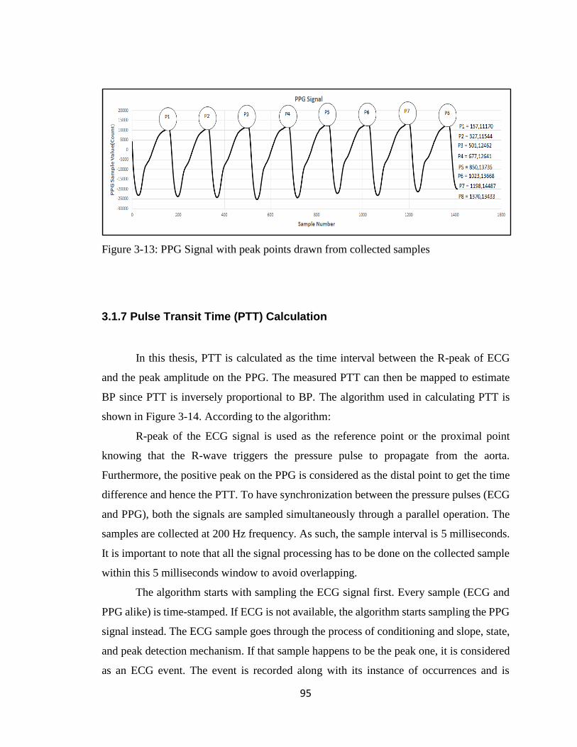
95
Figure 3-13: PPG Signal with peak points drawn from collected samples
3.1.7 Pulse Transit Time (PTT) Calculation
In this thesis, PTT is calculated as the time interval between the R-peak of ECG
and the peak amplitude on the PPG. The measured PTT can then be mapped to estimate
BP since PTT is inversely proportional to BP. The algorithm used in calculating PTT is
shown in Figure 3-14. According to the algorithm:
R-peak of the ECG signal is used as the reference point or the proximal point
knowing that the R-wave triggers the pressure pulse to propagate from the aorta.
Furthermore, the positive peak on the PPG is considered as the distal point to get the time
difference and hence the PTT. To have synchronization between the pressure pulses (ECG
and PPG), both the signals are sampled simultaneously through a parallel operation. The
samples are collected at 200 Hz frequency. As such, the sample interval is 5 milliseconds.
It is important to note that all the signal processing has to be done on the collected sample
within this 5 milliseconds window to avoid overlapping.
The algorithm starts with sampling the ECG signal first. Every sample (ECG and
PPG alike) is time-stamped. If ECG is not available, the algorithm starts sampling the PPG
signal instead. The ECG sample goes through the process of conditioning and slope, state,
and peak detection mechanism. If that sample happens to be the peak one, it is considered
as an ECG event. The event is recorded along with its instance of occurrences and is

96
considered as the reference point. The algorithm goes for the second event on the ECG. If
the second event occurs, the difference between the ECG events is calculated, and if the
interval is within a specified limit (450 milliseconds to 1000 milliseconds, in reference to
R-R cycle), the interval is considered valid. During this interval, if there is one PPG peak
detected, which is also sampled simultaneously, the time difference between the reference
point and the instant of PPG peak detection is considered as PTT. This is considered one
R-R cycle and the process is repeated ten times. If the event interval is outside of the limit
or no PPG peak is detected within that event interval, or more than one PPG peak is
detected in that interval, no PTT is calculated and the instant of the second event (ECG
Peak) becomes the new reference point.
Simultaneously, the algorithm samples PPG signal and the sample goes through the
conditioning, slope, state, and peak detection mechanism as the ECG sample. If a peak is
detected, it is registered as a PPG event and the instant of occurrence is recorded. This peak
occurrence must be within the R-R cycle of the ECG and there must be only one peak
within that cycle. This event and its instant are used in the PTT calculation as mentioned
above.
The calculated PTT is also compared against a default limit and if the value lies
outside the limit, it is discarded. This way, for every R-R cycle, the algorithm calculates a
PTT for that cycle. All the calculated and valid PTTs are stored in an array. The valid PTTs
are averaged and the average value is used as the final PTT. During sampling the signals,
if the interface does not work or the algorithm fails to detect the peaks, a timeout is
triggered and is reported. For that, a reset counter is running to keep track of that scenario.
Since PTT is a timing aspect, as such, various timing windows and event counters
are implemented in the algorithm described above to keep track of the events and the
occurrences of events in terms of timing.

97

98

99

100

101
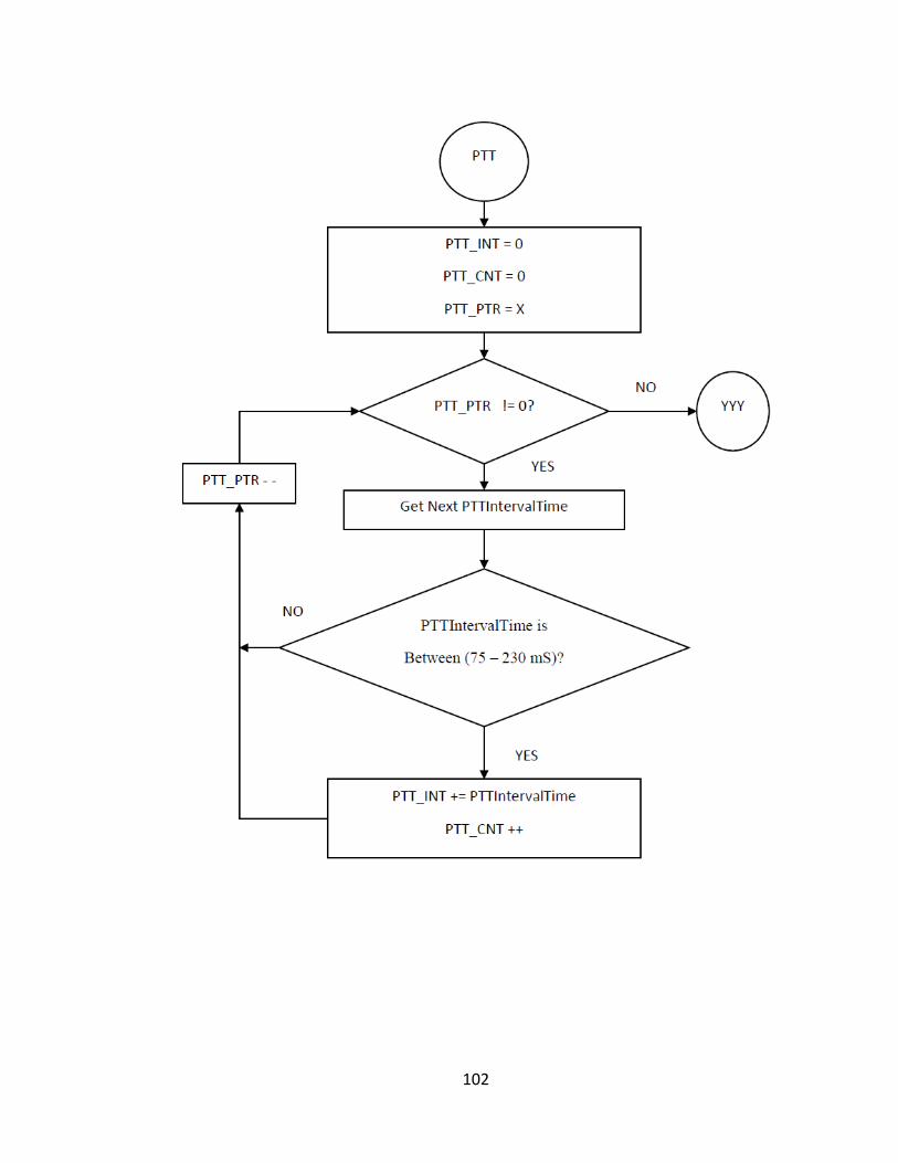
102

103
Figure 3-14: Flow diagram for Pulse Transit Time (PTT) calculation

104
3.2 Health Indices Calculation
The developed biosignal computing platform is meant to display and calculate
health indices, such as BP, SpO2, HR, and body temperature. The amplitude, cycle time, a
characteristic point on the biosignals play a vital role in calculating those health indices.
Once those parameters along with pulse transit time are available, it is just a matter of
putting those values into the calculation and estimates the desired health indices. The
methods and processes involved in calculating the health indices are described in the
following sub-sections:
3.2.1 BP Calculation
Calculating BP using PTT involves an indirect method consists of two phases,
namely training, and testing. And carried out offline. The training phase is involved in
developing a model, whereby, the testing phase is dedicated to verifying the developed
model. For that, BP is measured using a standard instrument (BP meter) and the
corresponding PTT is measured by the biosignal computing platform. The measurands are
then divided into two sets, training measurands, and testing measurands. Training
measurands are used to develop a regression model, relating BP and PTT, during the
training phase. The PTT values from the testing measurands are used in the developed
model to calculate BP, during the testing phase. Thus we have two sets of BP readings.
One is measured by the standard instrument, and the other is calculated by the computing
platform corresponding to each of the PTT readings in the training measurands. The
calculated BP values are then compared with the measured BP values and are subjected to
various statistical analyses, including correlation, mean error, and standard deviation of
errors among others. If the statistical results fall within the acceptable range, the regression
model thus developed would be implemented in the application and would enable
subsequent BP estimation when a future PTT is measured.
Following the above methodology, and to develop the parametric model for future
BP estimation through the proposed computing platform, PTT is calculated for a subject

105
by the system. In the same setting, BP is also measured from the subject using the standard
BP meter. Hence, the calculated PTT corresponds to this measured BP, which constitute
one sample point. The collected sample points will be used during the training and testing
phase and will be subjected to statistical analysis for verification as will be described in
detail in chapter 4. The flow chart of the BP estimation process is shown in Figure 3-15.

106

107
Figure 3-15: Flow diagram for BP estimation process
For the same subject, several sets of sample points are collected. The PTT
calculation and the BP measurements are conducted in an interleaved fashion. Using the
same procedure, enough sets of sample points are collected from numerous subjects.
A portion of the sample points thus collected are used to develop a model formula
(function relating PTT and BP) following the linear regression model using a third-party
application, such as Excel/Minitab, during the training phase. During the testing phase, the
remaining sample points along with the model developed in the training phase are used for
verification and statistical analysis of the developed model. Once satisfactory, the derived
model would then be coded in the system application for future BP measurements, when a
future PTT is measured by the proposed computing platform.

108
3.2.2 Blood Oxygen Saturation and Heart Rate Calculation
Blood oxygen saturation level is measured indirectly through monitoring the
changes in blood volume in the skin. For that, PPG is used to determine the oxygen
saturation level (SpO2) in blood. To do the measurement, the developed biosignal
computing platform is attached to a probe, which is a finger clip type. It has an LED on
one side and a photodetector on the other side. The flow of blood is heartbeat induced or
pulsatile in nature so the transmitted light changes with time. Red and infrared lights are
used to estimate oxygen saturation of arterial blood as described in section 2.2. The
computing platform also uses the PPG signal to extract the heart rate information of the
subject since PPG follows the cardiac cycle. The basic algorithms and processes involved
in calculating SpO2 and heart rate are shown in the flow chart as in Figure 3-16.
According to the flow chart, the calculation process starts with the initialization of
the PPG interface. The PPG samples are collected on an interrupt basis under program
control at five milliseconds intervals. Every collected sample is time stamped. PPG samples
are acquired for 10-12 cardiac cycles. In each acquisition, two PPG samples are retrieved.
One for red light (Red) and the other for infrared light (IR). Both samples are conditioned
and subjected to slope, state, and peak detection mechanism. Thus, the signals are followed
very closely to ascertain their respective peak points. As such, the signal’s maxima and
minima values are updated based on the latest sample amplitude and its state.
The process of collecting samples continues until the signal reaches its peak state.
At this point, the peak-to-peak values for the Red and IR light sources are calculated using
the values in Maxima and Minima variables. Then the ratio of these peak-to-peak values
is calculated. This is called R, the ratio of ratios as defined in section 2.2. The R-value is
used to retrieve the corresponding SpO2 from a lookup table.
Every time a peak is detected on the PPG signal, this is considered as an event and
the event is time-stamped. An event counter is also maintained to keep counting the number
of such events. The time difference between two such events is used to calculate the heart
rate. The time interval between two consecutive peaks in the PPG signal constitutes one
cardiac cycle. The number of such cardiac cycles per minute predicts the heart rate.

109
In one measurement session, several sets of SpO2 and heart rate are calculated using
the algorithm mentioned above and the average value for both parameters is used as the
ultimate value and is displayed. A reset counter is maintained in the application and if it
reaches a preset value before detecting the next peak on the signal, the algorithm times out
as shown in the flow diagram.

110

111

112

113
Figure 3-16: Flow diagram for SpO2 and Heart Rate calculation

114
3.2.3 Body Temperature Calculation
The developed biosignal computing platform can measure body temperature. For
that, an AFE (DS18B20) is added and connected to the System Controller through 1-wire
communication interface. The DS18B20 requires strict protocols to ensure data integrity.
The processes and algorithms involved in the protocol are shown in Figure 3-17.
All transactions on the 1-Wire bus begin with an initialization sequence. The
initialization sequence consists of a reset pulse transmitted by the system controller
followed by presence pulse(s) transmitted by the Temperature AFE. The presence pulse
lets the system controller know that the DS18B20 is on the bus and is ready to operate. If
the presence pulse is detected, the algorithm then issue appropriate ROM and MEMORY
command followed by the Convert T command. The system controller also sets the
interface at high impedance state. Following the issuance of the Convert T command, a
temperature conversion is performed and the thermal data is stored in the scratchpad
memory while the system controller is at wait state. Following the wait state, the system
controller issues reset pulse. Besides, checks the presence of the slave. Following that, the
temperature information is retrieved over the 1-Wire interface by issuing a Read
Scratchpad command. At this point, the reset sequence is again performed.
Using the above process, one byte of the temperature reading is collected and
stored. One temperature reading consists of several bytes of data depending on the
resolution used. Using the same sequence, all the bytes related to the temperature reading
are collected and processed to come up with the final temperature value in Celsius.
According to the flow chart, several such readings are collected and averaged. The
averaged value is also converted to Fahrenheit version. Temperature readings, in Celsius
and Fahrenheit, are displayed.

115

116

117

118
Figure 3-17: Flow diagram for Body temperature calculation

119
3.3 System Application: Architectural View
The integral part of any embedded system is the application running in it. Every
embedded system is designed and developed to implement a specific function and the
embedded application executes that function. For the proposed biosignal computing
platform, system software has been developed which is modular and real-time in nature to
implement all the functionalities. It can react to real-time scenarios and perform real-time
computing. Though the system application is not object-oriented, for representation
purposes, the architecture of the system application is shown using a class UML (unified
model language) diagram as in Figure 3.18.
The system application is divided into four major interrelated classes/modules, each
class with numerous data fields and methods (functions). They are Application Control,
AFE Management, Signal Processing, and Data Communication. The Application Control
module is the overall controller of the application. It implements an infinite loop in it
through which the user interacts with the application. This module is also vital to system
configuration and resource management. The AFE Management module is responsible for
managing and operating the various AFEs used in the design. The signal processing module
contributes the most by implementing novel algorithms and techniques to process
biosignals. Finally, the Data Communication module does all the data communication. The
modules interact with each other seamlessly and work as a feeder for the other. Each of
these modules is implemented through numerous function modules and described in more
detail in the subsequent sections. A generalized view of the system application is presented
in this chapter; the actual implementation is more comprehensive and complex in some
cases.
In addition to this system application, another android application has been also
developed in this thesis. It is to be installed and run on an android device. This android
application mainly for data communication between the developed biosignal computing
platform and a remote device.

120
Figure 3-18: System Application Architecture in class UML diagram

121
3.3.1 Application Control Class
The Application Control class is in total control of the application and its UML
diagram is shown in Figure 3-19. The application starts with the initialization of system
resources, all the AFEs, and other sub-systems. The initialization routines are categorized.
As such, the relevant peripherals are configured by the respective function modules under
the System-Init category. In this category, system resources like I/O ports, clock, interrupts,
uarts, timers are configured. Through AFE-Init, all the analog front ends are initialized and
set to operation by utilizing their programming features. The functions in AFE-Init thus
responsible for resource allocation, register initializations, and communication interface
settings for the AFEs. The initialization process could be very exhaustive. To give an
insight, for example, the initialization routines for PPG AFE involves the configuration of
fifty registers with default data just to start with. Each register is 24 bits in length, as such;
the configuration involves 1200 (50×24) bits of data. Each bit or a group of bits of those
registers has a purpose and function and they need to be initialized accordingly. The
registers can be categorized into four major groups, such as control, status, error, and result.
The functions in the App-Init class deal with the setting and definition of various filters
implemented in the application. Before entering into the infinite loop, the application also
initializes other subsystems including display unit.
Once initialization is complete, the application enters into an infinite loop. This is
the main engine of the application and is the user interface to the application. The structure
of the infinite loop is shown in Figure 3-20. In the loop, the application continuously keeps
reading the function switches, the user’s request. There are few function switches
implemented in the protoboard using push button switches. Each function switch represents
one of the functions (reading ECG, estimating SpO2, heart rate, body temperature, and
calculating PTT, etc.).
If one of the switches is pressed, the application acknowledges it and initiates the
execution of multiple function modules in the chain to get the intended job done. After
servicing the request, the application goes back to the read mode and the loop is repeated.
To prevent two or more switches to be active at the same time, a mutually exclusive
algorithm is implemented in the loop control code.

122
Figure 3-19: Architecture of Application Control in class UML diagram.

123
Figure 3-20: Structure of System Engine Loop.

124
3.3.2 AFE Management Class
The AFE management class of the system application is mainly responsible for self-
testing, calibration, and operation of the AFEs as shown in the UML diagram (Figure 3-
21). These functionalities have been divided into two phases, such as the pre-acquisition
and acquisition phase. In the pre-acquisition phase, the function modules prepare the AFEs
through self-testing and calibration processes. Based on the results of this pre-acquisition
process, the AFEs are calibrated by configuring its registers. Each of the control registers
in the AFE is configured through configuration routines. The configuration data is
determined in consultation with the datasheet concerning the test and calibration process.
The configuration exercise sets the dc operating voltage for the ADC. Besides, it also sets
other parameters on the signal path, such as the gain of the amplifier, cut-off frequency for
the filter, sampling frequency, decimation rate, and output data rate of the ADC. With these
settings, appropriate for the subject under test, samples are collected. The diagnostic
routines under this class, read the error and status registers to ascertain the state of the
AFEs. If errors are discovered, it is reported and readings are discarded. On the fly, the
acquired sample goes through a slope estimation process and the signal slope is calculated
dynamically. This dynamically calculated slope will be used as a threshold later to detect
signal features under the purview of a state machine implemented in the signal processing
module. Though the mechanism mentioned above is the same for all the AFEs, the signal
characteristics are different from each other. As such, there are three versions of the AFE
management module dealing with each of the AFE. At times, they overlap whenever there
is a need for such an association. Such as, during the process of PTT calculation.
During the signal acquisition phase, timing and event windows are set to keep track
of all the events and instances of the events. For that, every sample collected is time
stamped. For timekeeping, dedicated timers are configured and set to run and stop under
program control. For feature detection, events are recorded. For all these, necessary timing
and event function modules as shown in the UML diagram are defined in this AFE
management module. These function modules are responsible for event management and
record keeping. Once the timer and event-related parameters are set to run, the AFE

125
management module issue ‘START’ command to the AFE to start the signal acquisition
process.
Figure 3-21: Architecture of AFE Management Module in class UML diagram.
Once instructed, the AFE starts the process of signal acquisition, conditioning, and
digitizing the sample. The AFE management module keeps polling the ‘Finish’ flag coming
from the AFE once the sample data is available. The sample data is then collected and
stored by respective function modules as shown in the UML diagram. The just acquired
sample will be further processed by the function modules in the signal processing class.

126
3.3.3 Signal Processing and Computing Class
The signal processing and computing class is the backbone of the system
application. The biosignal processing is done through the functions in this class. This class
consists of numerous function modules as shown in Figure 3-22. The signal-processing
task is divided into three main blocks, such as signal conditioning, state detection, and
feature extraction. These tasks are implemented using the functions defined in this class.
The conditioning of the signal starts with the collection of a biosignal sample, which is
done by the AFE management module. The sample then goes through a multi-stage
filtering process. In the process, numerous filters, such as pulse filters, slope filters, high
pass, and low pass filters are implemented as shown in the UML diagram. The filtered
sample is then passed to the next function modules to determine its slope, state, and edge
using state of the art algorithms and techniques using some purpose-built functions. Using
the information (slope, state, and edge), the signal characteristic points (minima, maxima)
of the signal are updated using the function modules defined in signal processing class.
Event counting and timekeeping are important aspects of signal processing in the
system application. To calculate various health indices, it is paramount to detect
characteristic points on the biosignal as well as the instant of detection. As such, a state
machine is implemented in the Signal Processing class for event detection, counting, and
timekeeping. Few function modules are dedicated to this class to implement the state
machine. There are some functions defined in this class for event and time management as
shown in Figure 3-22. For timekeeping and event management, Timer1 of the system
controller is used. The Tick rate for the timer is set at one millisecond. If the time-stamped
sample happens to be a characteristic point, one can know the instant of occurrence of that
event. After every event, the corresponding time or event parameter is updated and the
value is used in the calculation. As such, the function modules enable one to calculate the
interval time between events, duration of an event, and the number of events in a time
window.

127
Figure 3-22: Architecture of Signal Processing module in class UML diagram.

128
3.3.4 Data Communication and Display Class
The data communication and display class of the system application is dealing with
all sorts of data communication between the function modules within the application and
between the computing platform and the external world. For physical data communication,
the computing platform transmits data either to the terminal or to the android device. The
system controller has built-in UART (Universal Asynchronous Receiver Transmitter)
interfaces. UART A is used to communicate with the terminal program running on a
personal computer (PC) and UART B is used to communicate with the Bluetooth interface.
As such, the data communication class is divided into two sections, one is dealing with
terminal and the other is dealing with an android device. The functions implemented in this
class are shown in the class UML diagram (Figure 3-23).
Like any other peripheral device of the system controller, UART A and UART B
need to be initialized. Through various function modules, parameters such as baud rate,
data bit size, parity, number of stop bits, and flow control are set through parameter setting
function as shown in Figure 3-23. Dedicated functions are also defined in this class for data
transmission and reception. Once initialized, UART A is set to run, on a demand basis.
However, the interface is always available for data reception, which is on an interrupt basis.
UART B of the system controller is dedicated to the Bluetooth interface. Through
the function modules defined in data communication class, UARTB-BTLE (Bluetooth low
energy) interface is initialized and set to run. Parameters, such as peripheral name, service,
resource, private service, and characteristics are set through purpose-specific functions as
shown in the UML diagram. Through these initialization functions, the BTLE is configured
as a peripheral device, and as a data provider, as Server. Besides, the UART interface in
BTLE is also configured.
Another set of functions is defined in this class for advertisement, connection,
authentication, and data transfer as shown in the UML diagram. Once the BTLE is
configured, under the purview of these functions, the BTLE is set to run and start
advertising to the remote devices. Once connected after authentication, all the health
indices estimated by the computing platform are transmitted to the peer device through
private service. For that, few private services and private characteristics are generated in

129
the function modules. When all the parameters are transmitted, the BTLE module stops
advertising and gets disconnected from the remote device under the control of
acknowledgment and termination related function defined in the data communication class.
The data fields for this class include txString, rxString, rescanBtle, btleCmd, and others are
declared and used as shown in Figure 3-23. It also includes a function to carry out data
display.
Figure 3-23: Architecture of Data Communication module in class UML diagram.
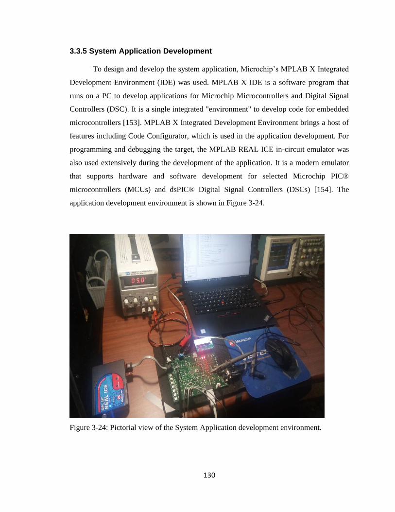
130
3.3.5 System Application Development
To design and develop the system application, Microchip’s MPLAB X Integrated
Development Environment (IDE) was used. MPLAB X IDE is a software program that
runs on a PC to develop applications for Microchip Microcontrollers and Digital Signal
Controllers (DSC). It is a single integrated "environment" to develop code for embedded
microcontrollers [153]. MPLAB X Integrated Development Environment brings a host of
features including Code Configurator, which is used in the application development. For
programming and debugging the target, the MPLAB REAL ICE in-circuit emulator was
also used extensively during the development of the application. It is a modern emulator
that supports hardware and software development for selected Microchip PIC®
microcontrollers (MCUs) and dsPIC® Digital Signal Controllers (DSCs) [154]. The
application development environment is shown in Figure 3-24.
Figure 3-24: Pictorial view of the System Application development environment.

131
3.4 Android Application: Architectural View
Due to technological development in the communication arena, especially in
wireless communication, it is possible to diagnose and care for patients from distance. As
such, the proposed biosignal computing platform houses a Bluetooth interface to cater for
that. The proposed system can estimate various health indices and transmit those wirelessly
to the android phone. The system application contains a data communication and display
class to control and operate the BTLE module as mentioned in section 3.3.4. For the
android phone, an android application has been developed as a proof of concept. The flow
chart of the developed android application is shown in Figure 3-25.
In short, the flow diagram starts with, by setting the component list tree and the
events. Events are buttons, such as START, STOP OnClickListeners and vary in terms of
functionalities (scanning, read, cease the application, etc.). Also, it sets all the callback
routines as shown in the diagram. The application then enables Bluetooth adapter, manager,
and Bluetooth scanner to set the Bluetooth interface running. When the START button is
clicked, the application starts the process of scanning. First, it checks the event and if it is
for discovering (scanning), it prepares a filter list. The filter list includes the name and
MAC (Medium Access Control) address of the remote device (the computing platform)
and starts scanning.
According to the flowchart, if the scanning process produces a result (discover a
remote device) and matches with the desired device name, the device name and MAC
address is retrieved from the scan result and is displayed on the corresponding components
on the screen. Then the connection process starts. Once connected, the service discovery
process starts. The characteristics and their properties are retrieved and notification on
change for the characteristics is set. So, if there are changes in the values of the desired
characteristics (health indices) in the remote device, the application is notified.
At this point, the application waits for the notification as shown in the flowchart.
Once notified, the application reads the characteristics and displays the same on the display
component. The application structured in an infinite loop so that the process continues.
There is an EXIT button, upon selection, the application gets disconnected from the remote
device and the application ends.

132
Start
Set the Component Tree
Set OnClick Listener
Enable Bluetooth Adapter
Enable Bluetooth Manager
Enable Bluetooth Scanner
Any Event
(START)? XXX NO
Get the Event
YES
Discover Event
(Scanning)?
AAA
YES
XXX
NO

133

134

135
Figure 3-25: Architecture and signal flow of Android Application.

136
For proof of concept, the developed android application was installed on an android
phone (version 6.0 Marshmallow, API level 23) and was set to run. Health data were
collected from the subject and were sent to the android phone on a real-time basis, which
is shown in Figure 3-26.
Figure 3-26: Pictorial view of the Android Application in operation.

137
3.5 System Hardware: Architectural View
The general layout of the system hardware is given in Figure 3-27. It consists of a
Microcontroller, which is the system controller, biosignal specific AFEs, and a radio
transceiver. The radio interface is a low energy Bluetooth module for reliable data transfer
between the computing platform and the android smartphone.
Figure 3-27: Functional decomposition of the biosignal computing platform
In the prototype, in the center, there is the system controller surrounded by three
AFEs. They are for, ECG, PPG, and body temperature. The dotted arrow indicates the
possibility of the future expansion of the system by adding more AFEs specific to other
biosignals. This design approach gives rise to an integrated single-board computer system
yet open for future expansion.
The AFEs are themselves a mixed-mode programmable processor, specifically,
designed for signal acquisition and conditioning of a specific biosignal. They are placed
between the sensors and the system controller and thus working as a feeder circuit. The

138
primarily conditioned biosignals from the AFEs are sent to the system controller using a
serial communication interface, such as a serial peripheral interface (SPI) or a one-wire
interface. The ECG and PPG AFEs are connected through SPI, while the body temperature
AFE is connected through a one-wire interface. The Bluetooth interface is connected to
the system controller through one of its built-in UART interfaces.
As far as the signal path is concerned, biosignals from the subjects are acquired,
conditioned, and digitized by the programmable AFEs. The conditioned data ends up at the
system controller through the SPI bus. The system controller is left with the task of further
conditioning, processing, and calculation. The calculated health indices are then sent to an
android phone through the radio interface.
3.5.1 Hardware Design Specifications
There are three main building blocks in the hardware design. They are system
controller, analog front ends, and the Bluetooth interface as a radio transceiver.
PIC24FJ256GA406, an extreme low-power Microcontroller, is used as the system
controller. The analog front ends (AFEs) comprise of three highly integrated AFEs. The
complete analog front end for a specific biosignal has been built into that mixed-mode
processor by integrating the necessary programmable hardware modules. The three AFEs
used in the design are ADS1293 (ECG), AFE4400 (PPG), and DS18B20 (Temperature).
For data communication, the RN4020 Bluetooth Low Energy module is used. The
specifications for each of the modules are described below:
3.5.2 System Controller: PIC24FJ256GA406
The system controller is in the center of the developed system. It is implemented
through PIC24FJ256GA406, an ultra low power, high performance, and cryptographic
central processing unit (CPU) from Microchip. It comes with 256k of program memory,
and 16k of data memory. This controller has multiple power management options for

139
extreme power reduction. VBAT (Backup Battery) mode allows the device to transition to
a backup battery mode for the lowest power consumption with the Real-Time Clock
Calendar (RTCC). Deep Sleep allows near total power-down with the ability to wake-up
on external triggers. Sleep and Idle modes selectively shut down peripherals and/or core
for substantial power reduction and fast wake-up. Doze mode allows CPU to run at a lower
clock speed than peripherals. Alternate Clock modes allow on the fly switching to a lower
clock speed for selective power reduction. It is also worthy to note its current consumption
at Deep Sleep, which is surprisingly very low. With watchdog timer (WDT), it is only 270
nA @ 3.3V typical. With the RTCC module on, it is 400 nA @ 32 kHz, 3.3V typical. At
Deep Sleep, the current is only 40 nA, 3.3V typical [155].
PIC24FJ256GA406 has several communication interfaces, such as multiple SPI, i2c
(inter-integrated circuit), parallel port, and 1-Wire, supporting both serial and parallel
communications. It helps provide seamless communication with the SPI compatible AFEs.
Each SPI interface is used to connect to one of the AFEs, specifically, ECG and PPG AFEs.
The body temperature AFE is connected through the 1-Wire interface. The other
characteristic of PIC24FJ256GA406 is its peripheral pin select (PPS) feature. This allows
programmable pin assignment among the peripherals and thus improves design flexibility.
It comes with a graphic display with 60 segments, each with 8 (eight) columns.
PIC24FJ256GA406 has 4 UARTs with 4 levels deep first in first out (FIFO) buffer.
3.5.3 Analog Front Ends (AFEs)
Analog front ends in the developed system are implemented using highly
integrated, state of the art mixed-mode programmable processors. These AFEs are
biosignal specific and responsible for biosignal acquisition, condition, and digitization. The
hardware of the AFE comprises multi-stage amplifiers, filters to amplify the tiny biosignals
and filter out unwanted signals, including motion artifacts. Signal parameters in the signal
path, such as, gain, cut-off frequency, sampling frequency, decimation factor, resolution,
and output data rate (ODR) among others are set under program control to get the optimum
results. This programmability feature provides significant flexibility in the design of
medical instrumentations. Besides, being able to implement a complete analog front-end

140
processing in a single mixed-mode controller increases system accuracy and reduces
overall power consumption. The AFEs are interfaced with the system controller through
the SPI bus. Through this interface, the AFEs are initialized and controlled. Under program
control, the AFEs can be instructed to start the process of biosignal acquisition and
conditioning. Once the conditioned data is available, the AFE notify the system controller
by changing a status line (Data Ready). The Data Ready status line is used as an external
interrupt source for the system controller. Upon notification, the system controller collects
the conditioned data through the SPI interface.
3.5.3.1 ADS1293 (ECG AFE)
The ADS1293 is a fully integrated analog front-end ideally suited for ECG signal
conditioning, and application. Every signal chain parameter inside the AFE is
programmable. For ECG, the actual differential signal between the electrodes in any lead
configuration is ±5 mV in magnitude and 0.05 Hz to 150 Hz in frequency. The skin-
electrode interface introduces a dc offset of approximately 300 mV. Also, a common-mode
voltage of approximately 1.4 V can be picked up by the human body due to power lines.
The actual ECG signal magnitude along with the resolution required from the ECG signal
determines the dynamic range of the front-end. The frequency content of the ECG signal
determines the bandwidth requirements.
According to the datasheet [156], the ADS1293 incorporates all features commonly
1required in portable, low-power medical, sports, and fitness electrocardiogram (ECG)
applications. With high levels of integration and exceptional performance, the ADS1293
enables the creation of scalable medical instrumentation systems at significantly reduced
size, power, and overall cost. The ADS1293 features three 24 bits resolution channels
capable of detecting 0.143 uVolts (2.4 V/ (224 – 1)) change in signal amplitude with a
sampling frequency of 204.8 kHz. Each channel can be independently programmed for a
specific sample rate and bandwidth allowing users to optimize the configuration for
performance and power. All input pins incorporate an EMI filter. Moreover, can be routed
to any channel through a flexible routing switch. Flexible routing also allows independent
lead-off detection, right-leg drive, and Wilson/Goldberger reference terminal generation

141
without the need to reconnect leads externally. The main features of ADS1293 are shown
in Table 3-1.
Table 3-1: Features of ADS1293 (ECG AFE)
3.5.3.2 AFE4400 (PPG AFE)
The AFE4400 is a fully integrated analog front-end ideally suited for pulse oximeter
applications [157]. The device consists of a low-noise receiver channel with an integrated
analog-to-digital converter (ADC), an LED transmit section, and diagnostics for sensor and
LED fault detection. The device is a very configurable timing controller. This enables the
user to have complete control of the device timing characteristics. It can communicate
seamlessly through the SPI interface and thus compatible with the system controller used
in the design. AFE4400 is a complete AFE solution for the acquisition and conditioning of
PPG signal and thus chosen in designing TasDiag. It has a 22-bit resolution, which equates
to 0.286 uVolts (1.2 V/ (222 - 1)) with a 95 Db channel dynamic range. And with a
maximum signal sampling frequency of 80 kHz.
The PPG signal is made of two distinct components. The AC component represents
the light absorption in the arterial blood, which is superimposed on a DC signal
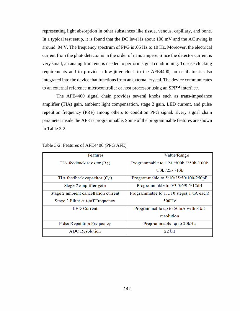
142
representing light absorption in other substances like tissue, venous, capillary, and bone.
In a typical test setup, it is found that the DC level is about 100 mV and the AC swing is
around .04 V. The frequency spectrum of PPG is .05 Hz to 10 Hz. Moreover, the electrical
current from the photodetector is in the order of nano ampere. Since the detector current is
very small, an analog front end is needed to perform signal conditioning. To ease clocking
requirements and to provide a low-jitter clock to the AFE4400, an oscillator is also
integrated into the device that functions from an external crystal. The device communicates
to an external reference microcontroller or host processor using an SPI™ interface.
The AFE4400 signal chain provides several knobs such as trans-impedance
amplifier (TIA) gain, ambient light compensation, stage 2 gain, LED current, and pulse
repetition frequency (PRF) among others to condition PPG signal. Every signal chain
parameter inside the AFE is programmable. Some of the programmable features are shown
in Table 3-2.
Table 3-2: Features of AFE4400 (PPG AFE)

143
3.5.3.3 DS18B20 (1-Wire® Digital Thermometer)
The DS18B20 is a fully integrated analog front end that provides temperature
readings. The core functionality of the DS18B20 is its direct-to-digital temperature sensor.
The resolution of the DS18B20 is configurable (9, 10, 11, or 12 bits), with 12-bit readings.
This equates to a temperature resolution of 0.5°C, 0.25°C, 0.125°C, or 0.0625°C. In terms
of readings, it has an accuracy of ±0.5 0C from -10 0C to +85 0C. DS18B20 is a fully
integrated analog front end suited for thermostatic controls, consumer products,
thermometers, or any thermally sensitive system [158]. The protocol consists of several
types of signaling on one line: such as, reset pulse, presence pulse, write 0, write 1, read 0,
and read 1. All of these signals, except the presence pulse, are initiated by the bus master.
The 1-Wire bus is a system, which has a single bus master (system controller) and one or
more slaves. The DS18B20 behaves as a slave. The protocol for accessing the DS18B20
via the 1-Wire port is initialization, ROM function command, Memory function command,
and transaction/data command.
Information is sent to/from the DS18B20 over a 1-Wire interface so that only one
wire (and ground) needs to be connected from the system controller to a DS18B20. Power
for reading, writing, and performing temperature conversions can be derived from the data
line itself with no need for an external power source. Its multidrop capability simplifies
distributed temperature sensing applications. Some of the features of DS18B20 are shown
in Table 3-3.
Table 3-3: Features of DS18B20 (Temp AFE)

144
3.5.4 Radio Transceiver (RN4020)
The developed biosignal computing platform, in addition to, biosignal computing
also capable of data sharing. For that, a Bluetooth interface is implemented in the proposed
design. The radio transceiver circuitry consists of an RN4020 Bluetooth® Low Energy
Module. It is a single Bluetooth Smart module, which complies with Bluetooth Core
Specification v4.1. Through its high-speed UART interface, this module can be configured
to act as either a central or a peripheral when establishing a connection. This module
supports 13 public profiles and 17 public services, which are adopted by the Bluetooth
Special Interest Group (SIG). For all supported profiles and services, the RN4020 module
can be configured to act as a server and client at the same time. Furthermore, the RN4020
module supports the private Microchip Low-energy Data Profile (MLDP), which provides
an asynchronous serial data connection between two RN4020 devices. Finally, the
Microchip RN4020 module also supports a user-defined private profile/service.
The system controller uses one of its UART interfaces to connect with the BTLE
module with a 115200-baud rate. It has been configured as a peripheral and acts as a server.
The system controller transmits health indices to a nearby smartphone through this BTLE
interface. All control takes place through ASCII commands and their parameters.
According to the datasheet [159], all commands are divided into the following types:
- Set/Get Commands
- Action Commands
- Characteristic Access Commands
- Private Service Configuration Commands
- Microchip MLDP Commands
- RN4020 Scripting Commands
- Remote Commands
- DFU (Device Firmware Update) Commands

145
3.6 System Hardware: Implementation
Proteus 8.2 Professional is a single application with many service modules offering
different functionality (schematic capture, PCB layout, etc.). The wrapper that enables all
of the various tools to communicate with each other consists of three main parts. They are
application framework, common database, and live netlist. This is the framework, the
container, which hosts all of the functionality of Proteus. ISIS (Intelligent Schematic Input
System), the schematic capture module in Proteus, ARES (Advanced Routing and Editing
Software), the PCB layout module in Proteus, and 3DV (3-D visualizer) all open as tabbed
windows within this framework and therefore all have access to the common database
[160]. In the design and development of the biosignal computing platform, Proteus has
been used as a schematic editor and for PCB layout.
The ISIS schematic capture module is used to draw the complete biosignal
computing platform circuit and then test it interactively, all from within the same piece of
software. The computing circuit then subjected to interactive simulation through the design
environment. The circuit also goes through the process of annotation and netlist
compilation. The circuit schematic is also checked through inbuilt electrical rules check
mechanism to check the integrity and accuracy of the design. Meanwhile, ISIS retains a
host of features aimed at the PCB designer and using that feature the design was exported
to ARES (Advanced Routing and Editing Software) for PCB production.
The hardware design process involves a few phases. Such as, designing the circuit
(schematic sheets), PCB layout, making the PCB, populating the PCB, and testing the
protoboard. The proto board is consists of six design units, these are, MCU, ECG, PPG,
Temperature, Radio, and Power. Each of the units was implemented on a separate
schematic sheet using Proteus schematic editor. All the sheets are connected through the
inter-sheet input/output signal path. A brief description of each of the design sheet is
described in the subsequent sections. The schematic sheets are available in Appendix A.

146
3.6.1 Schematic Sheet: MCU
The MCU schematic sheet mainly deals with the system controller and its
supporting sub-systems. The system controller is realized through PIC24FJ256GA406
Microcontroller from Microchip. It is a 16-bit processor with 64 pins. The system clock
can be provided by one of four sources (Primary, FRC, LPRC, and Secondary Oscillator).
The MCU design sheet is shown in Appendix A (Figure A-1).
In the design, an 8 MHz oscillator is connected between the OSCI and OSCO pins
as a primary oscillator (POSC). PIC24FJ256GA406 family devices include a versatile PLL
(Phase Lock Loop) block, which is used in the design. Since two cycles of the clock are
equivalent to one instruction cycle, the internal instruction cycle clock, FCY is 16 MHz,
which is calculated as follows:
FCY = (source clock) × 4 (PLL Factor)) / 2 (3.5)
= (8 MHz × 4)/2 = 16 MHz
Most of the input/output pins of the Microcontroller are remappable, a very useful
feature of the Microcontroller used in this design. Using this feature, any remappable I/O
pin can be assigned to any functions and any peripherals, making the deign experience
flexible. The available remappable input/output pins (RP0 ... RP30) are distributed among
all the used peripherals through the peripheral pin select (PPS) scheme. The remappable
I/O pins are mainly divided into four major groups to interface with AFEs (ECG, PPG, and
Temp), display unit, Bluetooth, and UARTs. The function switches are connected to port
pins RF0, RD7, RD1, and RG2 as shown in the schematic sheet. Status LEDs are connected
to RD0, RF1, and RF2 output pins. To reduce the effect of noise, multiple decoupling
capacitors are used on the power pins (Pins 10, 26, 38, 57). The Microcontroller operates
at 3.3V, which is sourced from the power sheet. For system reset and over-voltage
protection, a protection circuit is implemented and connected to the 𝑀𝐶𝐿𝑅 (Pin 7) of the
Microcontroller. An in-circuit serial programming (ICSP) interface is added (across PGC
and PGD pins) to program the Microcontroller. Multiple test points (T1 … T25) are also

147
implemented in the MCU circuit to monitor signal status and voltage levels. These test
points are monitored by connecting them to the oscilloscope probes.
3.6.2 Schematic Sheet: ECG
The ECG design sheet houses the ECG analog front end, which is responsible for
ECG signal acquisition, conditioning, and digitization. It has a two-interface circuitry. One
for connecting with the ECG electrodes and the other to communicate with the system
controller as shown in Appendix A (Figure A-2). The ECG AFE is implemented through
ADS1293 from Texas Instruments. It is connected in a 3-lead configuration using two
channels. In this configuration, the right arm (RA), left arm (LA), left leg (LL), and right
leg (RL) are connected to the IN1, IN2, IN3, and IN4 pins (Pin1…Pin4) respectively.
The ADS1293 uses the common-mode detector block to measure the common-
mode of the subject’s body by averaging the voltage of input pins IN1, IN2, and IN3 and
uses this signal in the Right Leg Drive (RLD) feedback circuit. The output of the RLD
amplifier is connected internally to the IN4, which is connected to the right leg electrode,
to drive the common-mode of the subject’s body. Pins 15 to 20 are connected to the system
controller. Specifically, pin 16 (CSB) is used for chip select and pins 17 to 19 (SCLK, SDI,
and SDO) are used for the SPI interface. These pins are used as part of the serial peripheral
interface (SPI). Pin 20 (DRDYB) is used as an external interrupt input to the system
controller (Pin 16, RB0) through inter sheet signal, ECG_DRDYB. Once data is available,
this pin becomes active low and triggers interrupt. The AFE is set to run on its clock by
connecting a crystal oscillator of frequency 4.096 MHz between pin XTAL1 and XTAL2.
The input pins (IN1…IN4) are connected to the electrodes through the ECGCONN
interface. All the input traces are passed through zero ohm resistors, in case there is a need
for impedance matching. A push-button switch (SW2) is added to the circuitry and
connected to the RSTB pin to induce manual reset. To set various operating voltage levels
at designated pins as suggested by the datasheet, passive components are added to the
circuit. Necessary pull-up resistors (R27, R22) are added to keep the logic level as required.
Multiple bypass capacitors are also added on the power pins to ground the noise. The power
line to the circuit is conditioned through L1 (a ferrite bead) before applying to power pins.

148
The supply voltage for this sheet is 3.3V, sourced from the power sheet. Critical pins of the
device are connected to the Test points for signal monitoring through an oscilloscope.
3.6.3 Schematic Sheet: PPG
The PPG (Oximetry) interface is implemented through the Oximetry design sheet.
In the center of the design, AFE4400 from Texas Instruments is used as shown in Appendix
A (Figure A-3). This AFE is meant for PPG signal acquisition, conditioning, and
digitization. Again, the circuit has two interfaces, one for sensor and the other for the
system controller. The AFE is connected to the sensor through the PPGCONN interface.
There are four input traces. Two of them belong to the transmit section and connected to
pin TXN and TXP respectively. The other two traces belong to the receiver section and
connected to pin INP and INM respectively. The receive traces between the sensor
connector and the AFE4400 are voltage common-mode (VCM) shielded to help reduce
noise and improve signal quality. All the four traces between the sensor and PPG AFE are
overvoltage protected as shown in the figure. The sensor mainly consists of LEDs and
photodiodes. The transmit pins (TXP, TXN) are connected to the LEDs while the receive
pins (INP, INM) are connected to the photodiode. TXP, TXN is fast-switching lines. As
such, is routed away from INP and INN lines. All the traces go through zero ohm resistors,
in case there is a need for impedance matching. The device can draw high-switching
currents from the LED_DRV_SUP pin. As a precaution, a decoupling capacitor C26 is
connected to the pin at the nearest distance possible.
The AFE4400 is set to run on its clock. As such, an 8 MHz oscillator is connected
between pin XIN and XOUT. The power line to the circuit is conditioned through a ferrite
bead (L2) to suppress noise due to electromagnetic interference. To set various operating
voltage levels at designated pins as suggested by the datasheet, passive components are
added to the circuit. Necessary pull-up resistors (Pin 29, Pin 20) are added to the circuit to
keep the logic level at default. The supply voltage for this sheet is 3.6V and sourced from
the power sheet.
Pins 21 to 29 are connected to the system controller. Pins 21 to 23 are for diagnostic
purposes. Pins 24 to 26 are part of the SPI interface. Through this interface, AFE4400 and

149
system controller communicates with each other. The system controller programs and
operates the AFE through this interface. The AFE also uses the same interface to send its
data to the system controller. Pin 27 (SPISTE) works as a chip select for the AFE4400. The
ADC_RDY (Pin 28) is connected to the system controller as an external interrupt input.
Once data is available, this pin becomes active high and triggers an external interrupt. The
AFE is reset by the system controller through RESET (Pin 29).
3.6.4 Schematic Sheet: Temperature
This design sheet houses several circuitry, such as temperature AFE, function
switches, and the LCD unit as shown in Appendix A (Figure A-4). The Temperature AFE
is implemented through DS18B20 from the Dallas semiconductor. Information is sent
to/from the DS18B20 over a 1-Wire interface so that only one wire (and ground) is
connected to the system controller. The TEMPCONN houses three pins (GND, DQ, and
VDD). The device can be powered either from a parasite (capacitor) or from an external
source (VDD). In this design, VDD is used to supply power to the AFE. For the DS18B20
to be able to perform accurate temperature conversions, sufficient power must be provided
over the DQ line when a temperature conversion is taking place. Since the operating current
of the DS18B20 is up to 1.5 mA, the DQ line has been provided with the 4.7k pull-up
resistor (R29) to provide sufficient drive. The DQ (Pin 2) of the AFE is connected to the
system controller through trace TEMP_SDA and ends at pin 36 (RG3) of the system
controller.
The same design sheet also houses the display controller, which is implemented
through NHD-C0216CU, chip-on-glass (COG) liquid crystal display (LCD) module. It
features 2 × 16 characters with a built-in ST7032-0 D controller. The pins can be divided
into two categories. Namely, data bus and control bus. The data bus is made of 8-bit
bidirectional data lines (pin 7 to 14). The control bus is made of four lines (pins3 to 6). Pin
1, and 2 (LED+, LED-) are for intensity control and connected to VDD through a zero-
ohm resistor. The parallel data bus is connected to the system controller on its PORT E
pins (RE0 … RE7). The control bus is connected to the system controller on its PORT G

150
pins (RG6 … RG9). The system controller programs the display controller through the
control bus while it sends the parallel data to the display unit through the data bus.
The biosignal computing platform offers various functionalities to the users. Such
as PTT calculation, ECG measurement, SpO2 calculation, and body temperature
measurement. These functionalities can be selected through push button switches (SW1 –
SW7) known as function switches. Those switches are implemented in this design sheet as
shown in Appendix A (Figure A-4). Each switch is connected to the system controller on
its input port pins. All the input lines are conditioned through a voltage divider circuit to
provide proper logic level to the system controller to ascertain the logic level. On the same
sheet, a dual in-line package (DIP-4) switch is also added to provide miscellaneous inputs
to the system controller.
3.6.5 Schematic Sheet: Communication
The Communication (Radio) schematic sheet houses the communication interface
of the computing platform as shown in Appendix A (Figure A-5). It includes a radio
transceiver and a UART interface for data communication. For radio, a Bluetooth interface
is implemented in the design sheet. The UART interface is for communicating to a
terminal. The RN4020 Bluetooth low energy (BTLE) from Microchip is used. The
transceiver is controlled through input/output lines (i.e., physical device pins) and a UART
interface. The device pins can be divided into two groups. They are RN4020 control and
RN4020 UART interface.
The control pins WAKE_SW (pin 7), CMD/MLDP (pin 8), WAKE_HW (pin 15)
are used to place the BTLE module into different states. The three output pins (pin 10, 11,
and 12) to indicate its status. These control pins are connected to the system controller
output PORT pins (RD6, RD5, and RD4). As such, the device can be initialized and
controlled under the program. The status pins of the device are connected to the LEDs to
indicate various statuses, such as WAKE, EVENT, and CONN (Connect). The CONN
output pin is also traced back to the system controller (RF3) for monitoring purposes. The
universal asynchronous receiver transmitter (UART) is the main control interface for the

151
RN4020 module. Its UART interface is connected to UART3 of the system controller. The
system controller sends all the commands and receives a response from the RN4020 device
through UART3. The default RN4020 UART configuration is shown in Table 3-4. In the
configuration, flow control is not used but provision for that is available in the circuitry.
The unused pins of the device are to be mentioned in ARES to avoid errors.
Table 3-4: RN4020 UART Configuration
Parameter Value
Baud Rate 115200
Data Bits 8
Parity None
Stop Bits 1
Flow Control No
For communicating with a terminal for data streaming, a second UART interface is
added to this design sheet. UART2 of the system controller is used for this purpose.
UART2 is interfaced with the MAX3232 device, which is a multichannel RS-232 Line
Driver/Receiver With ±15-kV ESD Protection. The device provides the electrical interface
between an asynchronous communication controller and the serial-port connector. Two
pins of the system controller (pin 44, 45) are configured as U2RX and U2TX through
peripheral pin select. No flow control signals used in the interface. The charge pump and
four small external capacitors (C21, C39, C40, and C41) allow operation from a single 3-
V to 5.5-V supply. UART2 is also configured as Table 3.4. A 9 pin D Connector (CONN-
D9F) is added to the design sheet to be connected with the terminal through RS-232 cable.
Pin 5 of the connector, the ground pin, is connected to the ground through a 10-ohm resistor
(R44).

152
3.6.6 Schematic Sheet: Power
The Power sheet takes care of all the power needs of the computing platform. The
platform uses various AFEs including the system controller with different power
requirements. Two voltage sources are required for the computing platform. They are 3.3V
and 3.6V respectively. As such, two voltage regulators are used to cater to two output
voltages. For that, two MCP1825T regulators are used in the design as shown in Appendix
A (Figure A-6).
The MCP1825/MCP1825S is a 500 mA low dropout (LDO) linear regulator that
provides high current and low output voltages. The MCP1825 comes in a fixed or
adjustable output voltage version, with an output voltage range of 0.8V to 5.0V. The
MCP1825/MCP1825S is made stable by using ceramic output capacitors that inherently
provide lower output noise and reduce the size and cost of the entire regulator solution. As
such, a one μF of output capacitance (C32 and C42 respectively) are connected at the output
pin, VOUT (PIN 4), to stabilize the LDO. The input to the LDO, VIN (pin 2), can be
provided from two mutually exclusive input sources. Two input sources are provided in
the circuitry. They are BATTPWR (Battery source) and USBPWR (USB source). A P-
channel MOSFET (Q1) is used to control the battery and for load management. The input
voltage source is conditioned through bypass capacitors (C30, C31) and further by C9 and
C17.
For adjustable Vout, the output voltage is connected to the ADJ (pin 5) input
through a resistor divider that sets the output voltage regulation (OVR) value. In the design,
the output voltage is adjusted using the formula provided by data sheet [161] as below:
Vout = 𝑉𝑎𝑑𝑗 ( 𝑅1+𝑅2
𝑅2 ) (3.6)
Where:
R1 and R2 are the resistors connected at the output pin of the regulator.
Vout = LDO output voltage
Vadj = Adj pin voltage (typically, 0.41 V).
The allowable range for resistor R2 is from 10 kΩ to 200 kΩ. Solving the equation for R1
yields the following:

153
R1 = 𝑅2 ( 𝑉𝑜𝑢𝑡−𝑉𝑎𝑑𝑗
𝑉𝑎𝑑𝑗 ) (3.7)
In the design sheet, R1 is represented by a series combination of R47 and R48 for
the upper LDO (U6) while R49 and R50 for the lower LDO (U8). R2 is represented by R34
for the upper LDO while R28 for the lower LDO. Few test points (T17, T18, and T19) are
provided in the design sheet to help trace the output voltage levels. Two LEDs (LD7 and
LD8) are added to provide the visual presence of the voltages. Few ground points are also
added for easy access to reference points.
3.7 Printed Circuit Board (PCB) Design
There are many basic rules and good practices to follow, but apart from that, PCB
design is a highly creative and individual process [162]. ARES (Advanced Routing and
Editing Software) forms the PCB layout module of the Proteus design suite and offers a
netlist based PCB design complete with a suite of high-performance design automation
tools [163]. As mentioned, ISIS, the schematic editor of Proteus is used to create all the
schematics mentioned above. The same design is exported for production with ARES.
During the PCB layout, the overall design is further verified through the design rule
checker (DRC) and connectivity rule checker (CRC). Using the design rule manager of
ARES, various design parameters, such as, clearances (pad-pad, pad-trace, and trace-trace),
layer assignment for routing, trace style, and others are set.
To keep the power traces clean, clear, and free from noise interference, the PCB
was made using four layers. The components are on the top layer. The traces are in the top
and bottom layers. The inner layer (inner 1) is the power plane while the other inner layer
(inner 2) is holding the ground plane. ARES includes an auto-placer module, an addition
that in combination with the auto-router makes it possible to create PCBs almost entirely
automatically. For the proposed design, some of the critical components are placed
manually and auto-placing the rest. The most tedious, error-prone, and time-consuming
part of the traditional electronics development process is undoubtedly routing the PCB. As
a result, it is in this area that the greatest benefits of Electronic Design Automation are to
be found. In this design, the auto-router feature of ARES is used heavily but occasionally,
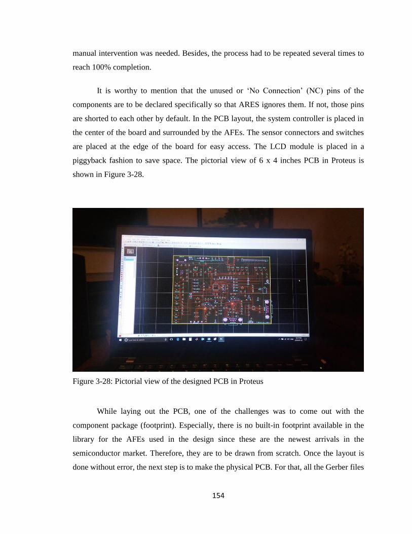
154
manual intervention was needed. Besides, the process had to be repeated several times to
reach 100% completion.
It is worthy to mention that the unused or ‘No Connection’ (NC) pins of the
components are to be declared specifically so that ARES ignores them. If not, those pins
are shorted to each other by default. In the PCB layout, the system controller is placed in
the center of the board and surrounded by the AFEs. The sensor connectors and switches
are placed at the edge of the board for easy access. The LCD module is placed in a
piggyback fashion to save space. The pictorial view of 6 x 4 inches PCB in Proteus is
shown in Figure 3-28.
Figure 3-28: Pictorial view of the designed PCB in Proteus
While laying out the PCB, one of the challenges was to come out with the
component package (footprint). Especially, there is no built-in footprint available in the
library for the AFEs used in the design since these are the newest arrivals in the
semiconductor market. Therefore, they are to be drawn from scratch. Once the layout is
done without error, the next step is to make the physical PCB. For that, all the Gerber files

155
were generated along with components list and a PCB was made through a third party. The
pictorial view of the physical PCB (top layer) is shown in Figure 3-29 and the bottom layer
is shown in Figure 3-30. The next step is to populate the PCB with the intended
components.
Populating the PCB with the generated component list comes up with a bigger
challenge. The reason is all the components used in the design are surface mounted devices.
Soldering them manually on the board is not an easy task. Also, the AFEs, system controller
and other devices are either Quad Flat Pack No-Lead (QFN) or Thin Quad Flat Pack No-
Lead (TQFN), or Very Thin Quad Flat Pack No-Lead (VQFN) type package configuration.
Figure 3-29: Pictorial view of the physical PCB (Top layer)

156
Figure 3-30: Pictorial view of the physical PCB (Bottom layer)
QFNs are difficult because all the connections are on the bottom of the chip and a
lot of passions and precautions are required when soldering is done manually [164]. Some
versions have small extensions of these connections that wrap around the bottom corner
and come up the edge a little. As if, they have foot but no toe. Soldering those devices
manually becomes even harder. Anyway, with some hurdles, a PCB was populated with
the components and a prototype board was made. The prototype board is shown in Figure
3-30.
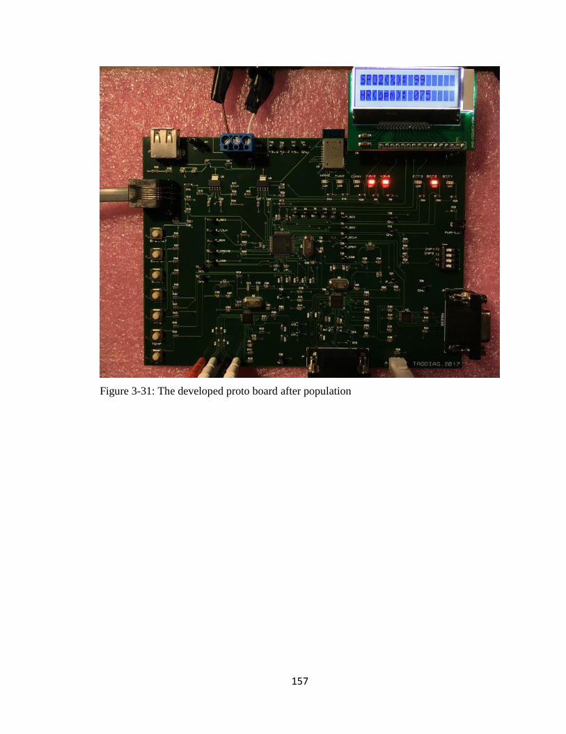
157
Figure 3-31: The developed proto board after population

158
Chapter 4 : Research Results
The developed biosignal computing platform, named TasDiag, is a multi-modal
system for computing various health indices. It can read biosignals, such as, ECG and PPG
data of a subject and utilizing these biosignals, TasDiag can estimate both systolic blood
pressure (SBP) and diastolic blood pressure (DBP). It is also capable of measuring heart
rate (HR), oxygen saturation level (SpO2), and body temperature. For design verification
and performance measurement, various health data were acquired from subjects. The
acquired data are analyzed and studied. This study has been reviewed by the University of
Ontario Institute of Technology (UOIT) Research Ethics Board and approved (REB #
14522). The participants were briefed about the purpose and processes of the study
according to the REB #14522 document and informed consent was obtained in writing
from the participants.
TasDiag is verified against each of the health indices (SBP, DBP, SpO2, HR, and
body temperature). For that health data were collected from subjects using TasDiag and
industry-standard instruments, such as Omron BP meter, Datex patient monitor, and
Veridian digital thermometer. The collected data were subjected to various statistical
analyses. Statistical analysis for performance and accuracy are compared between TasDiag
and the standard instruments in terms of mean, standard deviation, mean absolute
percentage error, mean absolute error, correlation of coefficient, probability (p-value), and
coefficient of determination. Besides, rigorous analysis is also performed in terms of bias,
scatter plot, histogram, and Bland-Altman plot.
4.1 Measuring Procedure
A total of 30 (22 males and 8 females) subjects participated in the study in various
ways. The respective (male and female) number of participants is solely based on their
interest, convenience, and availability. Also, the number of participants varied because it
was not possible to carry all the test instruments to the participant’s premises. The
demographic data of the participants are shown in Table 4-0. Health data (sample points)
are collected from the subjects and used for verification of various health indices. As for,

159
BP, 570 sample points were collected from the subjects. Each sample point consists of one
PTT reading calculated by TasDiag and two BP readings (SBP and DBP) by Omron BP
meter. As such, 1710 data points were collected for the BP parameter. Considering the
importance of BP parameter in human health,
Table 4-0: Demography of the Participants
Age Group (18-24) Age Group (25-39) Age Group (40-59) Age Group (60-65)
5 (M) + 2 (F) 8 (M) + 2 (F) 7 (M) + 4 (F) 2 (M)
TasDiag is verified against two profiles, one is individual (individual analysis) and the
other is a group (group analysis). As such, two sets of BP readings are collected. One set
is used to create an individual profile and the other one is to produce a group profile. The
individual profile is created by collecting long term sample points from one subject. For
the group profile, sample points were collected from 30 participants. In the group profile,
6 to 15 sample points were collected from a subject on the same day or where possible on
different days of the study period. The verification process for the BP parameter has two
phases, such as training and testing. The collected data has been divided into two parts:
training and testing sample points. Training sample points are used to develop the
regression model relating to BP and PTT, during the training phase. The PTT values from
the testing sample points are used in the developed model to calculate BP during the testing
phase. Against each PTT, there is a corresponding calculated BP. As such, we have two
sets of BP, one is measured by Omron BP meter, and the other is calculated by TasDiag as
outlined in section 3.2.1 (BP Calculation).
For verifying other health indices, such as SpO2, HR, and body temperature, data
readings are recorded from the subjects using standard instruments and by TasDiag. The
readings are then subjected to comparative study through statistical analysis. The specific
standard diagnostic tools used in the study are Omron cuff-based digital BP meter (Model:
BP765CAN), a Datex CT/DI Monitor for recording SpO2 and HR, and a digital
thermometer from Veridian healthcare.

160
4.2 Data collection for Model Establishment and Verification
To estimate SBP and DBP based on PTT, a mathematical model needs to be
established first. For model establishment and subsequently for verification, data (sample
points) from the subjects were collected as distinct sample points. Up to 6 to 15 sample
points from each subject were collected, depending on their availability. Each sample point
consists of three readings, SBP, DBP, and PTT. BP readings were measured by the Omron
BP meter and the corresponding PTT were TasDiag. A minimum of six sample points was
collected from each subject on a given day with three sample points in each session. There
was a time gap between the sessions. For some subjects, up to 15 sample points were
collected on consecutive days or when they were available. The collected sample points
are used for group profiling. Data was also collected from an individual subject to create
an individual profile. For individual profiles, sample points were obtained from an
individual on a daily basis for a long period of time.
During each data collection session, three sample points were recorded. During
each recording, ECG and PPG signals, equivalent to 10 R-R cycles were collected and the
corresponding calculated PTT value by TasDiag was recorded. Systolic and diastolic blood
pressures were also measured using the BP meter at the end of the PTT calculation. This
constitutes one cycle of data collection or one sample point consists of one PTT reading
and two BP readings (SBP and DBP). The process was repeated two more times, as such,
three sample points were collected in one session. The BP meter was programmed in
average mode, so that, individual and average readings were available. This helps to discard
unusual observations during data sorting. Though it is customary to measure the pressure
at the same time as the PTT is measured to preserve accuracy, it is not feasible since the
inflation and deflation of the cuff influence the heart rate. As such, a consecutive
measurement was adopted instead of simultaneous measurement. The readings were
collected while the subject was in sitting condition. A pictorial view of the data collection
session is shown in Figure 4-1.
Using the above procedure, for BP measurement, a total of 360 sample points were
collected for group profiling from 30 subjects. And after initial sorting, 341 sample points
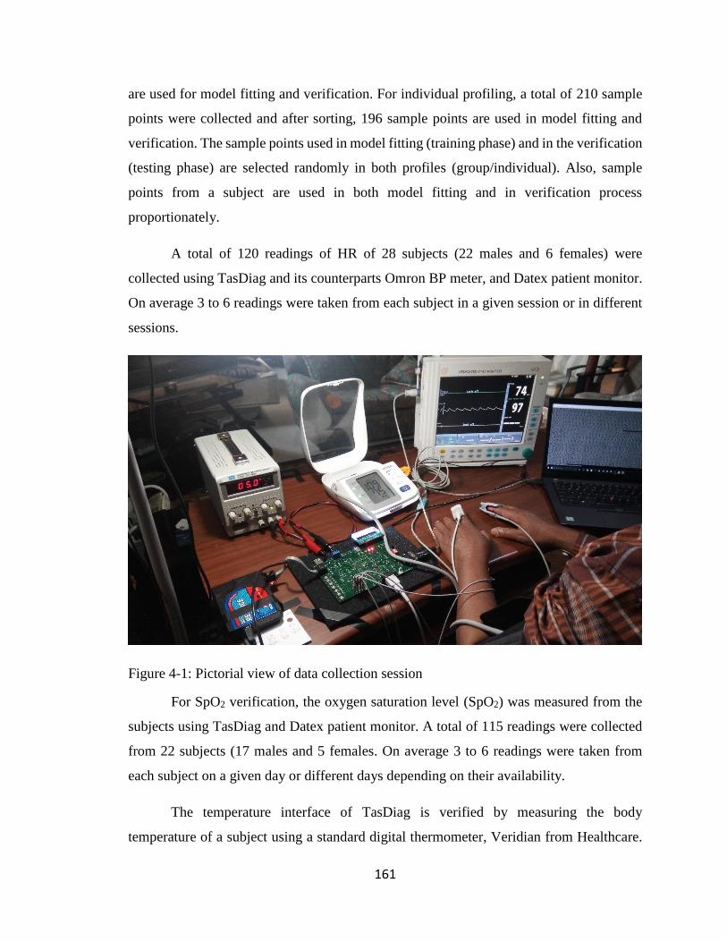
161
are used for model fitting and verification. For individual profiling, a total of 210 sample
points were collected and after sorting, 196 sample points are used in model fitting and
verification. The sample points used in model fitting (training phase) and in the verification
(testing phase) are selected randomly in both profiles (group/individual). Also, sample
points from a subject are used in both model fitting and in verification process
proportionately.
A total of 120 readings of HR of 28 subjects (22 males and 6 females) were
collected using TasDiag and its counterparts Omron BP meter, and Datex patient monitor.
On average 3 to 6 readings were taken from each subject in a given session or in different
sessions.
Figure 4-1: Pictorial view of data collection session
For SpO2 verification, the oxygen saturation level (SpO2) was measured from the
subjects using TasDiag and Datex patient monitor. A total of 115 readings were collected
from 22 subjects (17 males and 5 females. On average 3 to 6 readings were taken from
each subject on a given day or different days depending on their availability.
The temperature interface of TasDiag is verified by measuring the body
temperature of a subject using a standard digital thermometer, Veridian from Healthcare.

162
Parallelly, body temperature was also measured using TasDiag by placing the thermal
sensor under the tongue of the subject. A total of 50 readings were collected using both
devices.
4.3 Validation and Performance Comparison
For performance and accuracy measurement, health data were collected using
TasDiag and its counterpart and are subjected to comparison. Each of the health index
estimated by TasDiag is verified and compared against its counterpart. And a comparative
study follows as below:
TasDiag acquires vital biosignal such as ECG and PPG to calculate various health
indices. The same ECG and PPG signal of the subject can be channeled to a monitor for
clinical overview by the health professionals. To see the quality of the acquired signals,
ECG and PPG samples are assembled and plotted. Figures 4-2 and 4-3 show the ECG and
PPG waves as acquired by TasDiag from a subject. The plots show that the derived signals
are clean, distinct, and free from noise. It also shows the effects of artifacts, as well as,
common-mode interferences are minimal. Figures 4-4 and 4-5 depict the same set of signals
as provided by clinically standard medical equipment. Both sets of signals resemble each
other very much and support the relevance of TasDiag.
Figure 4-2: ECG wave derived by TasDiag
43160004317000431800043190004320000432100043220004323000
0 200 400 600 800 1000
AD
C O
utp
ut
Co
un
t V
alu
e
Sample Number
Scatter Plot: ECG Signal

163
Figure 4-3: PPG wave derived by TasDiag
Figure 4-4: ECG wave derived by clinical device
-20000
-15000
-10000
-5000
0
5000
10000
-50 150 350 550 750 950 1150 1350 1550 1750
AD
C O
utp
ut
Co
un
t V
alu
e
Sample Number
Scatter Plot : PPG Signal

164
Figure 4-5: PPG wave derived by clinical device
The BP parameter is tested and verified very extensively. It is tested from the
systolic and diastolic points of view. Besides, BP is tested using two profiles, namely,
group and individual. In the group profile, a total of 341 sample points are used for model
fitting and verification. Out of 341 sample points, 190 sample points (Training Sample
Points) are used to develop the regression model during the training phase and 151 sample
points (Testing Sample Points) are used for verification purposes during the testing phase.
The sample points used for both training and testing processes are shown in Appendix A
(Table A-3). As mentioned before, each sample point in the table represents one set of BP
readings (both systolic and diastolic) by Omron and the corresponding PTT reading by
TasDiag for a subject. Using the Training Sample Points in the table, two regression lines
(models), one for SBP and the other for DBP are plotted as shown in Figure 4-6 and Figure
4-7. They are the scatter plots of SBP and DBP against PTT respectively. The correlation
coefficient, R, measures the strength of the relationship between two variables, in this case
between BP and PTT. The correlation coefficient between SBP and PTT is 0.920 and
between DBP and PTT is 0.85. The correlation coefficients are quite high and indicate a
strong relationship exists between the variables. The strong relationship is also evident

165
from the graphs as the points in Figure 4-6 and Figure 4-7 lie almost along the straight line.
The line passing through the data points in the scatter plots is the regression line that relates
BP and PTT. And represents the parametric model: BP =K1
PTT + K2 . During the testing
phase, PTT values from the Testing Sample Points (from Appendix A, Table A-3), are used
in the above model to calculate SBP and DBP. This way, two sets of BP readings are
obtained, one calculated by TasDiag against each of the PTT and the other measured by
Omron. Table A-4 (in Appendix A) shows both the readings along with their differences
in the group profile.
Figure 4-8 and Figure 4-9 show the scatter plots of SBP and DBP readings
measured by Omron and calculated by TasDiag as described above. They show that there
is a perfect correlation as the points in Figure 4-8 and Figure 4-9 lie almost along the
straight line. Figure 4-10 and Figure 4-11 represents the Bland-Altman plot of the BP
differences (Omron – TasDiag) against the mean averages of both devices for systolic and
diastolic readings. Horizontal lines are drawn at the mean difference and at the limits of
agreement, which are defined as the mean difference plus and minus 1.96 times the
standard deviation of the differences. These plots are used to assess the agreement between
Omron and TasDiag by calculating the bias. The bias is calculated by taking the average
of the differences between the readings of the Omron device and TasDiag. In this case,
SBP bias is -0.471 mmHg and DBP bias is 0.117 mmHg. The bias is represented by
drawing a line parallel to the x-axis, corresponding to zero differences. It shows that on
average, TasDiag measures 0.471 mmHg more than the Omron device in SBP
measurement and 0.117 mmHg less than Omron in DBP measurements. The Bland-Altman
plots also show that in 95% cases, the differences in readings lie inside the range of
confidence interval (±1.96SD limits), which is between 8.909 mmHg to -9.852 mmHg in
the case of SBP and between 8.48 mmHg to -8.247 mmHg in the case of DBP. Figure 4-
12 and 4-13 show the histograms of the relative errors of SBP and DBP readings
respectively. The relative error is calculated by:
ABS (BPOmron – BPTasDiag)/BPOmron

166
The graphs show most of the errors lie within 5.0847 mmHg for SBP, and 6.0893 mmHg
for DBP.
Table 4-1 and Table 4-2 shows the statistical performance characteristics between
Omron and TasDiag. According to Table 4-1, the mean systolic and diastolic BP readings
calculated by TasDiag are 113.80 mmHg and 76.96 mmHg with a standard deviation of
±12.25 mmHg and ±5.87 mmHg respectively. The mean systolic and diastolic BP readings
by the Omron device are 113.33 mmHg and 77.079 mmHg with a standard deviation of
±13.71 mmHg and ±7.985 mmHg respectively. The comparison results in Table 4-2
indicate that the calculations by TasDiag are close to the true value of the standard
instrument (Omron) with a mean absolute percentage error of 3.63% and 4.88% for SBP
and DBP respectively. As such, the accuracy of TasDiag for SBP and DBP measurements
are 96.37% and 95.12% respectively. The coefficient of correlation between Omron and
TasDiag is 0.938 for SBP, and 0.853 for DBP, which indicates a strong relationship. In
terms of the ρ-value, the probability, which is ≤ .0001 strongly supports the notion that the
correlation coefficient is statistically significant. The Coefficient of determination, R2,
measures the predictability of the dependent variable from the independent variable. In that
respect, according to the table, the value for the coefficient of determination is 0.88 and
0.73 for SBP and DBP respectively, which are high. If we can predict y variable from x
variable then we would have a coefficient of determination of 1. Usually, the coefficient of
determination of 0.70 is considered good [165]. Table 4-2 also shows the mean absolute
error, mean error, and standard deviation of the error between Omron and TasDiag. The
mean absolute error is 4.11 mmHg and 3.70 mmHg for SBP and DBP respectively and the
mean error is -0.47 mmHg for SBP and 0.11 mmHg for DBP. In terms of standard
deviation, they are 4.78 mmHg and 4.26 mmHg respectively. Based on the American
Association for the Advancement of Medical Instrumentation (AAMI) requirements (5±8
mmHg), these values are well within the acceptable range.
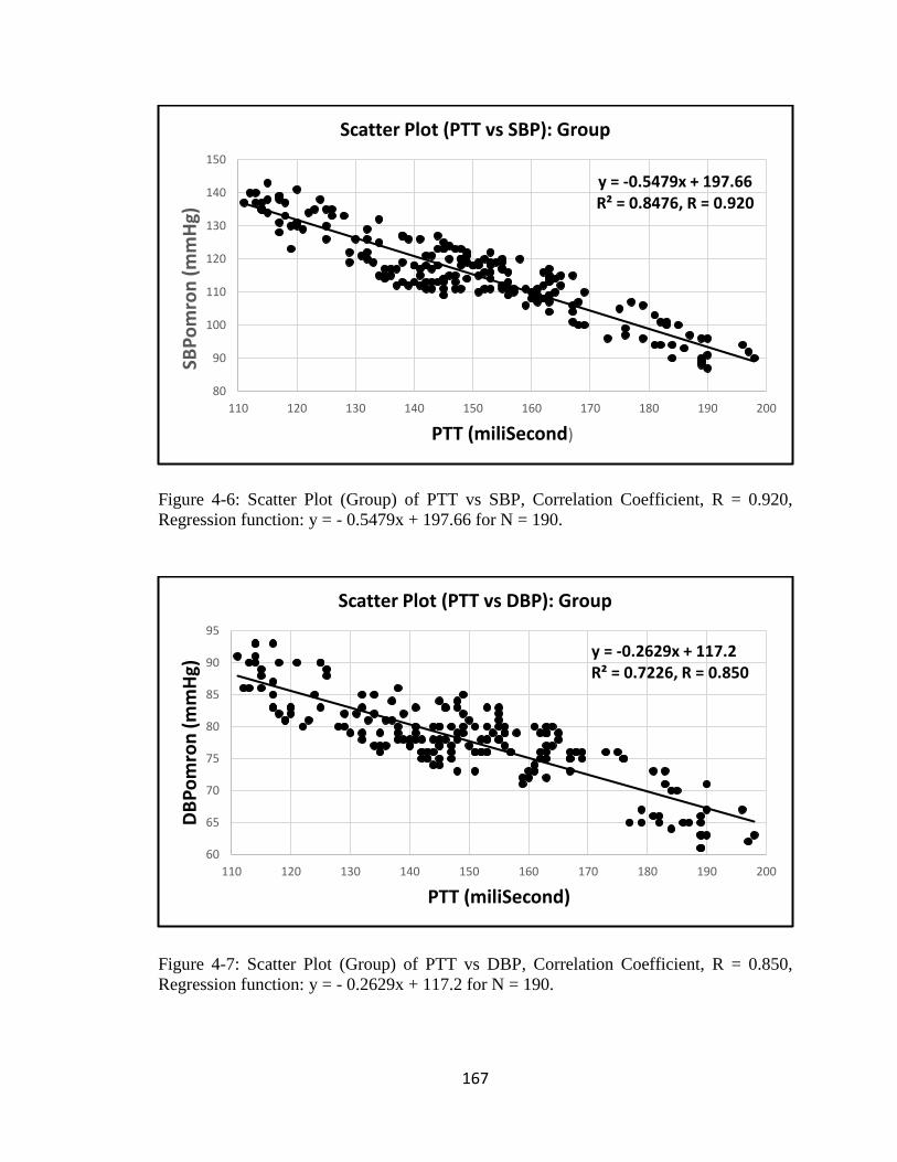
167
Figure 4-6: Scatter Plot (Group) of PTT vs SBP, Correlation Coefficient, R = 0.920,
Regression function: y = - 0.5479x + 197.66 for N = 190.
Figure 4-7: Scatter Plot (Group) of PTT vs DBP, Correlation Coefficient, R = 0.850,
Regression function: y = - 0.2629x + 117.2 for N = 190.
y = -0.5479x + 197.66R² = 0.8476, R = 0.920
80
90
100
110
120
130
140
150
110 120 130 140 150 160 170 180 190 200
SBP
om
ron
(m
mH
g)
PTT (miliSecond)
Scatter Plot (PTT vs SBP): Group
y = -0.2629x + 117.2R² = 0.7226, R = 0.850
60
65
70
75
80
85
90
95
110 120 130 140 150 160 170 180 190 200
DB
Po
mro
n (
mm
Hg)
PTT (miliSecond)
Scatter Plot (PTT vs DBP): Group

168
Figure 4-8: Scatter Plot (Group) of SBPomron vs SBPtasdiag, Correlation Coefficient, R
= 0.938, Regression function: y = 0.8381x + 18.817 for N = 151.
Figure 4-9: Scatter Plot (Group) of DBPomron vs DBPtasdiag, Correlation Coefficient, R
= 0.853, Regression function: y = 0.6281x + 28.55 for N = 151.
y = 0.8381x + 18.817R² = 0.8802, R = 0.938
80
90
100
110
120
130
140
80 90 100 110 120 130 140
SBP
tasd
iag(
mm
Hg)
SBPomron(mmHg)
Scatter Plot(SBPomron vs SBPtasdiag): Group
y = 0.6281x + 28.55R² = 0.7281, R = 0.853
60
65
70
75
80
85
90
55 60 65 70 75 80 85 90 95
DB
Pta
sdia
g(m
mH
g)
DBPomron(mmHg)
Scatter Plot(DBPomron vs DBPtasdiag): Group

169
Figure 4-10: Bland-Altman Plot (Group) for SBP
Figure 4-11: Bland-Altman plot (Group) for DBP
-15
-10
-5
0
5
10
15
80 90 100 110 120 130 140 150 160
SBP
om
ron
-SB
Pta
sdia
g(m
mH
g)
Mean of SBPomron and SBPtasdiag(mmHg)
Bland-Altman Plot (SBP): Group
+1.96 SD
Mean
-1.96 SD
8.909
-0.471
-9.852
-10
-8
-6
-4
-2
0
2
4
6
8
10
55 60 65 70 75 80 85 90 95
DB
Po
mro
n -
DB
Pta
sdia
g(m
mH
g)
Mean of DBPomron and DBPtasdiag(mmHg)
Bland-Altman Plot (DBP): Group
+1.96 SD
Mean
-1.96 SD
8.481
0.117
-8.247

170
Figure 4-12: Histogram of the relative error for SBP: Group
Figure 4-13: Histogram of the relative error for DBP: Group

171
Table 4-1: Statistical comparison of performance-1 for BP (Group)
Table 4-2: Statistical comparison of performance-2 for BP (Group)
TasDiag is also tested against the individual profile. In the individual profile, 196
sample points are used for training and testing purposes. Like before, the verification
process for BP is divided into two phases, namely training and testing. In the training phase,
121 sample points (Training Sample Points) are used to develop the regression model and

172
in the testing phase, 75 sample points (Testing Sample Points) are used for verification
purposes. The sample points used for both training and testing processes are shown in
Appendix A (Table A-5). Using the 121 Training Sample Points in the table, two regression
lines, one for SBP and the other for DBP are plotted as shown in Figure 4-14 and Figure
4-15. They show the scatter plot of SBP and DBP readings against PTT respectively. The
correlation coefficient between SBP and PTT is 0.933 and between DBP and PTT is 0.849,
which is quite high and indicates a strong relationship. The strong relationship between the
readings also visible from the graphs as the points in Figure 4-14 and Figure 4-15 lie almost
along the straight line. During the testing phase, PTT values from the Testing Sample
Points (from Appendix A, Table A-5), are used in the regression equations developed
during the training phase to calculate SBP and DBP. This way, two sets of BP readings are
obtained, one calculated by TasDiag against each of the PTT and the other measured by
Omron. Table A-6 (in Appendix A) shows both the readings along with their differences
in the individual profile. Figure 4-16 and Figure 4-17 show the scatter plot of BP readings
by Omron against TasDiag. Again, there is clear evidence of a strong correlation between
the readings as the points in Figure 4-16 and Figure 4-17 lie almost along the straight line.
Figure 4-18 and 4-19 represent the Bland-Altman plots of BP differences (Omron –
TasDiag) against the mean averages of both devices for systolic and diastolic readings.
From the graphs, with 95% confidence, one can say that the differences in readings are
within the confidence interval (± 1.96 SD limits), which is between 6.507 mmHg to -7.14
mmHg for SBP and 5.755 mmHg to -5.188 mmHg for DBP. In this case, SBP bias is -
0.316 mmHg and DBP bias is 0.283 mmHg. That means on average TasDiag measures
.316 mmHg more than the standard equipment (Omron) in SBP measurement. For DBP
measurements, TasDiag measures .283 mmHg less than Omron. Figure 4-20 and 4-21 show
the histograms of the relative errors of SBP and DBP readings respectively. The graphs
show most of the relative errors lie within 6.08 mmHg for SBP, and 4.054 mmHg for DBP.
Table 4-3 and Table 4-4 show the statistical performance characteristics between
Omron and TasDiag in the individual profile. According to Table 4-3, the mean systolic
and diastolic BP readings by TasDiag are 115.72 mmHg and 77.83 mmHg with a standard
deviation of ±10.16 mmHg and ±3.81 mmHg respectively. The mean systolic and diastolic
BP readings by Omron are 115.40 mmHg and 78.12 mmHg with a standard deviation of

173
±10.81 mmHg and ±5.24 mmHg respectively. The comparison results in Table 4-4 indicate
that the calculation by TasDiag is close to the true value of the standard instrument (Omron)
with a mean absolute percentage error of 2.42% and 3.081% for SBP and DBP respectively.
As such, the accuracy of TasDiag for SBP and DBP measurements are 97.58% and 96.92%
respectively. The coefficient of correlation between the readings between TasDiag and
Omron is 0.947 for SBP, and 0.856 for DBP, which are very high. The probability factor
(ρ-value), which is ≤ .0001, strongly supports the notion that the correlation coefficient is
statistically significant. The coefficient of determination, R2, according to the table, is
0.896 and 0.732 for SBP and DBP respectively, which indicates strong predictability exists
among the readings. Table 4-4 also shows the mean absolute error, mean error, and
standard deviation of error between Omron and TasDiag. The mean absolute error is 2.77
mmHg and 2.40 mmHg for SBP and DBP respectively and the mean error is -0.31 mmHg
for SBP and 0.28 mmHg for DBP. In terms of standard deviation, they are 3.48 mmHg and
2.79 mmHg respectively. All these parameters comply with AAMI requirements. As such,
TasDiag has the potential for measuring BP constantly and non-invasively. By comparing
the statistical data given in Table 4-2 and Table 4-4, it can also be concluded that TasDiag
performs slightly better in the individual profile than in the group profile.

174
Figure 4-14 Scatter plot (Individual) of PTT vs SBP, Correlation Coefficient, R = 0.933,
Regression function: y = -0.57x + 200.16 for N = 121
Figure 4-15: Scatter plot (Individual) of PTT vs DBP, Correlation Coefficient, R = 0.849,
Regression function: y = -0.214x + 109.54 for N = 121
y = -0.57x + 200.16R² = 0.8706, R = 0.933
95
105
115
125
135
145
155
105 115 125 135 145 155 165 175 185
SBP
om
ron
(mm
Hg)
PTT (miliSecond)
Scatter Plot (PTT vs SBP): Individual
y = -0.214x + 109.54R² = 0.7223, R = 0.849
60
65
70
75
80
85
90
95
100 110 120 130 140 150 160 170 180 190
DB
Po
mro
n(m
mH
g)
PTT (miliSecond)
Scatter Plot (PTT vs DBP): Individual

175
Figure 4-16: Scatter plot (Individual) of SBPomron vs SBPtasdiag, Correlation Coefficient,
R = 0.947, Regression function: y = 0.8903x + 12.975 for N = 75
Figure 4-17: Scatter plot (Individual) of DBPomron vs DBPtasdiag, Correlation
Coefficient, R = 0.856, Regression function: y = 0.6231x + 29.158 for N = 75
y = 0.8903x + 12.975R² = 0.8963, R = 0.947
100
105
110
115
120
125
130
135
140
100 105 110 115 120 125 130 135 140 145
SBP
tasd
iag(
mm
Hg)
SBPomron(mmHg)
Scatter Plot(SBPomron vs SBPtasdiag): Individual
y = 0.6231x + 29.158R² = 0.7329, R = 0.856
70
72
74
76
78
80
82
84
86
88
65 70 75 80 85 90 95
DB
Pta
sdia
g(m
mH
g)
DBPomron(mmHg)
Scatter Plot (DBPomron vs DBPtasdiag): Individual

176
Figure 4-18: Bland-Altman plot for SBP: Individual
Figure 4-19: Bland-Altman plot for DBP: Individual
-10
-8
-6
-4
-2
0
2
4
6
8
10
100 105 110 115 120 125 130 135 140 145SBP
om
ron
-SB
Pta
sdia
g(m
mH
g)
Mean of SBPomron and SBPtasdiag(mmHg)
Bland-Altman Plot (SBP): Individual
+1.96 SD
Mean
-1.96 SD
6.507
-0.316
-7.14
-8
-6
-4
-2
0
2
4
6
8
70 72 74 76 78 80 82 84 86 88 90DB
Po
mro
n -
DB
Pta
sdia
g(m
mH
g)
Mean of DBPomron and DBPtasdiag(mmHG)
Bland-Altman Plot (DBP): Individual
+ 1.96 SD
Mean
- 1.96 SD
5.755
0.283
-5.188

177
Figure 4-20: Histogram of the relative error for SBP: Individual
Figure 4-21: Histogram of the relative error for DBP: Individual

178
Table 4-3: Statistical comparison of performance-1 for BP (Individual)
Table 4-4: Statistical comparison of performance-2 for BP (Individual)
TasDiag can measure heart rate (HR). The readings by TasDiag are compared and
verified against the readings by standard equipment such as Datex and Omron. Table A-7
(in Appendix A) shows the HR readings measured by TasDiag and Datex/Omron with
differences. For HR readings, two standard equipments were used and those readings are
denoted by Datex/Omron combination. A total of 120 readings were collected from 28

179
subjects. Figure 4-22 shows the scatter plot of HR readings of Datex/Omron against
TasDiag. The graph shows there is a perfect correlation between the readings as the points
in Figure 4-22 lie almost along the straight line.
Figure 4-23 shows the Bland-Altman plot of the differences in HR readings
(Datex/Omron – TasDiag) against the mean average readings of the devices. The Bland-
Altman plot shows that in 95% cases, the differences in readings lie inside the range of
confidence interval (±1.96SD limits), which is between 1.653 bpm to -2.087 bpm. In this
case, HR bias is -0.216 bpm. That means on average, TasDiag measures 0.216 bpm more
than the standard equipment (Datex/Omron) in HR measurements. Figure 4-24 shows the
histogram of the relative errors of HR readings by Datex/Omron and that of TasDiag, where
most of the relative errors lie within 1 bpm.
Table 4-5 and Table 4-6 give statistical performance characteristics between
Datex/Omron and TasDiag. Table 4-5 shows the mean HR reading by TasDiag is 78.14
bpm with a standard deviation of ±10.34 bpm and mean HR reading by Datex/Omron
devices is 77.93 bpm with a standard deviation of ±10.24 bpm. The statistical results in
Table 4-6 indicate that the measurements by TasDiag are close to the true value of the
standard instruments (Datex/Omron) with a mean absolute percentage error of 0.86%. That
means the accuracy of TasDiag for HR measurements is 99.14% which is very high. The
coefficient of correlation between the readings of TasDiag and Datex/Omron is 0.996,
which is super high and almost perfect. The probability factor (ρ-value), which is ≤ .0001
strongly supports the notion that the correlation coefficient is statistically significant. The
coefficient of determination, R2, according to the table, is 0.992, which indicates strong
predictability exists among the readings. Table 4-6 also shows the mean absolute error,
mean error, and standard deviation of the error between Datex/Omron and TasDiag. The
mean absolute error is 0.66 bpm and the mean error is -0.21 bpm. In terms of standard
deviation, it is 0.95, which is within the accuracy limits of ±5 bpm recommended by the
AAMI standard for heart rate meters [166].

180
Figure 4-22: Scatter plot of HR, Correlation Coefficient, R = 0.996, Regression function:
y = 1.0061x – 0.2574 for N=120
Figure 4-23: Bland-Altman plot for HR
y = 1.0061x - 0.2574R² = 0.9915, R = 0.996
55
65
75
85
95
105
115
55 60 65 70 75 80 85 90 95 100 105
HR
tasd
iag(
BP
M)
HRomron/datex(BPM)
Scatter Plot (HR)
-2.5
-2
-1.5
-1
-0.5
0
0.5
1
1.5
2
2.5
50 60 70 80 90 100 110HR
om
ron
-H
Rta
sdia
g(B
PM
)
Mean of HRdatex/omron and HRtasdiag(bpm)
Bland-Altman Plot (HR)
+1.96 SD
1.653
Mean
-0.216
-1.96 SD
-2.087

181
Figure 4-24: Histogram of the relative error for HR
Table 4-5: Statistical comparison of performance-1 for HR

182
Table 4-6: Statistical comparison of performance-2 for HR
Another important health index is the oxygen saturation level in the blood (SpO2).
TasDiag is designed to measure this important health index. The readings by TasDiag are
compared and verified against the readings by standard equipment such as Datex. Table A-
8 (in Appendix A) shows the readings measured by both the devices along with differences.
A total of 115 readings were collected from 22 subjects. Figure 4-25 represents the Bland-
Altman plot of SpO2 differences (Datex – TasDiag) against the mean average readings of
both devices. The Bland-Altman plot shows that in 95% cases, the differences in readings
lie inside the range of confidence interval (±1.96SD limits), which is between 1.443 % to
-2.382%. In this case, SpO2 bias is -0.469. That is, on average, TasDiag measures 0.469
units more than the standard equipment (Datex). Figure 4-26 shows the histogram of the
relative errors of SpO2 readings, where most of the relative errors lie within 1%.
Table 4-7 gives statistical performance characteristics between Datex and TasDiag.
According to the table, the mean reading of SpO2 by TasDiag is 97.157% with a standard
deviation of ±1.18. The mean SpO2 by Datex device is 96.68% with a standard deviation
of ±0.98. The statistical results in Table 4-7 indicate that the measurements by TasDiag are
close to the true value of the standard instrument (Datex) with a mean absolute percentage
error of 0.88%. That means the accuracy of readings by TasDiag for SpO2 measurements

183
is 99.12%, which is very high. Table 4-7 also shows the mean absolute error, mean error,
and standard deviation of the error between Datex and TasDiag. It shows that mean
absolute error is 0.85%, and the mean difference is -0.469%. In terms of standard deviation,
it is 0.97, which complies with the AAMI standard for SpO2 device performance (±3%)
[167].
Figure 4-25: Bland-Altman plot for SpO2
Figure 4-26: Histogram of the relative error for SpO2
-3
-2.5
-2
-1.5
-1
-0.5
0
0.5
1
1.5
2
2.5
94.5 95 95.5 96 96.5 97 97.5 98 98.5 99 99.5
SPO
2d
atex
-S P
O2ta
sdia
g(%
)
Mean of SPO2datex and SPO2tasdiag(%)
Bland-Altman Plot (SPO2)
+1.96 SD
1.443
Mean
-0.469
-1.96 SD
-2.382

184
Table 4-7: Statistical comparison of performance for SpO2
TasDiag is also designed to measure body temperature. The readings by
TasDiag are compared against the readings by a standard thermometer, Veridian, a digital
thermometer. Table A-9 (in Appendix A) shows the readings measured by both the devices
along with differences. A total of 50 readings were collected from an individual on a long
term basis. Few high-temperature readings are obtained using a simulated environment to
mimic fever conditions. Figure 4-27 is the scatter plot of temperature readings of Veridian
against TasDiag. The graph shows there is a perfect correlation between the readings as the
points in Figure 4-27 lie almost along the straight line. Figure 4-28 shows the Bland-
Altman plot of temperature differences (Veridian – TasDiag) against the mean average
readings of both devices. The Bland-Altman plot shows that in 95% cases, the differences
in readings lie inside the range of confidence interval (±1.96SD limits), which is between
0.683 0F to -0.374 0F. The temperature bias is 0.156. That is, on average, TasDiag measures
.156 0F less than the standard equipment (Veridian). Figure 4-29 shows the histogram of
the relative errors of temperature readings, where most of the relative errors lie within 0.33
0F. Therefore, with this minimal error, it is possible to replace the standard device with
TasDiag.
Tables 4-8 and 4-9 give statistical performance characteristics between Veridian
and TasDiag. Table 4-8 shows the mean temperature reading by TasDiag is 98.201 ᴼF with
a standard deviation of ±1.33 ᴼF and mean temperature reading by Veridian thermometer
is 98.358 ᴼF with a standard deviation of ±1.372 ᴼF. The statistical results in Table 4-9
indicate that the measurements by TasDiag are close to the true value of the standard
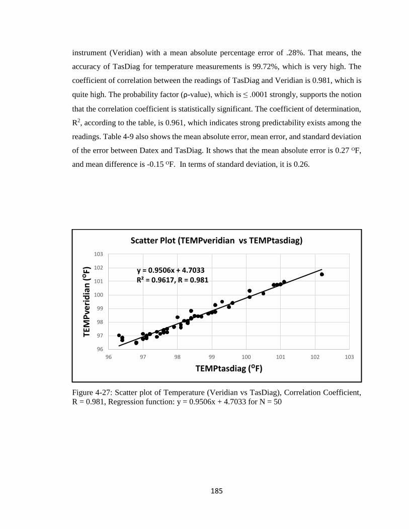
185
instrument (Veridian) with a mean absolute percentage error of .28%. That means, the
accuracy of TasDiag for temperature measurements is 99.72%, which is very high. The
coefficient of correlation between the readings of TasDiag and Veridian is 0.981, which is
quite high. The probability factor (ρ-value), which is ≤ .0001 strongly, supports the notion
that the correlation coefficient is statistically significant. The coefficient of determination,
R2, according to the table, is 0.961, which indicates strong predictability exists among the
readings. Table 4-9 also shows the mean absolute error, mean error, and standard deviation
of the error between Datex and TasDiag. It shows that the mean absolute error is 0.27 ᴼF,
and mean difference is -0.15 ᴼF. In terms of standard deviation, it is 0.26.
Figure 4-27: Scatter plot of Temperature (Veridian vs TasDiag), Correlation Coefficient,
R = 0.981, Regression function: y = 0.9506x + 4.7033 for N = 50
y = 0.9506x + 4.7033R² = 0.9617, R = 0.981
96
97
98
99
100
101
102
103
96 97 98 99 100 101 102 103
TEM
Pve
rid
ian
(ᴼF
)
TEMPtasdiag (ᴼF)
Scatter Plot (TEMPveridian vs TEMPtasdiag)

186
Figure 4-28: Bland-Altman plot for Temperature
Figure 4-29: Histogram of the relative error for Temperature
.
-0.8
-0.6
-0.4
-0.2
0
0.2
0.4
0.6
0.8
96 97 98 99 100 101 102 103
TEM
Pve
rid
ian
-TE
MP
tasd
iag
(ᴼF)
Mean of TEMPveridian - TEMPtasdiag (ᴼF)
Bland-Altman Plot (Temperature)
+1.96 SD
0.683
Mean
0.156
-1.96 SD
-0.374

187
Table 4-8: Statistical comparison of performance-1 for Temperature
Table 4-9: Statistical comparison of performance-2 for Temperature
4.4 Physical Parameters of TasDiag
TasDiag is a single board computer (SBC) and the physical dimension of TasDiag
is 6×4 inches in size and weighs 110 grams. The display unit is piggybacked and can be
separated. Without the display unit, the board weighs 90 grams. The system uses two
voltage levels such as 3.6 V and 3.3 V derived from a single source. The board can be
powered from a 5 Volt power source or a battery pack. It can also be powered from a USB
source with sufficient current (Approximately 150 milliamperes). The system draws

188
approximately 150 milliamperes while running in full swing including the 2×16 LCD
alphanumeric display module and the Bluetooth module on. During idle state, it draws
around 135 milliamperes. Therefore, the system can run without interruption, an ideal time
of 7.40 (1000/135) hours.
4.5 Comparison with Related Work
The non-invasive and continuous way of measuring health indices including BP
based on PTT is being pursued by other researchers too. Some researchers are focusing
their efforts on establishing models relating to BP and PTT, while the others are focusing
on designing systems to implement those models. In doing so, the researchers are following
various models, methods, and procedures though with a common goal of best realization
of PTT-based BP measurement.
The authors in [143] proposed a non-invasive continuous BP monitoring device
using a wearable body sensor network. Table 4-10 shows the comparison of TasDiag with
the device designed by Lin et al. According to the table, the comparative study has been
divided into three fields, namely, application, hardware, and statistics. In this
implementation, PTT is calculated via ECG and PPG signals collected from two different
sub-systems (Wristband, HR belt). As such, synchronization between these two signal
sources has become an issue and sometimes challenging to achieve precision. Rigorous
synchronization protocol needs to be implemented in the application, whereas no such
requirement is needed in TasDiag. Recalibration is an important aspect of PTT based BP
measurements, which is missing in [143], on the other hand, TasDiag has a comprehensive
recalibration mechanism in its application. TasDiag is a single board solution whereas the
device designed by Lin et al. [143] is a multi-board solution. The proposed system used
two Microcontrollers, two ADCs, and two Bluetooth devices and thus increases the cost,
size, and component counts of the system. The system consists of three parts: wristband,
HR belt, and a smartphone. The system in [143] has thus become a distributed system

189
whereas TasDiag is an integrated system. The system by Lin et al. must accompany a
smartphone to see the data on the screen, whereby TasDiag has a built-in display unit.
TasDiag can be placed on the wrist and fingertips while the said device has to be placed on
the chest and wrist which makes the subject uncomfortable.
In terms of statistical analysis, the results carried out by authors in [143], give a
mean absolute error of 4.46 mmHg, and a standard deviation of 6.49 mmHg for systolic
BP. For the same parameter, TasDiag gives a mean absolute error of 4.11 mmHg, and a
standard deviation of 4.78 mmHg. There is no mention of mean error of the proposed
system by Lin et al whereas, in the case of TasDiag, it is -0.47 mmHg for SBP, which is
well within the specification by AAMI. There is no mention of diastolic data for the said
system though TasDiag gives a mean absolute error of 3.70 mmHg, the mean error of 0.11
mmHg, and a standard deviation of 4.26 mmHg for diastolic BP. And comply with AAMI
specifications.

190
Table 4-10: Comparison with published work [143]

191
The authors in [144] presented a continuous and noninvasive BP monitoring system
working through WBSN composed of a photoplethysmographic sensor node located on the
forehead, and an electrocardiographic sensor node located on the chest. Table 4-11 is the
comparative study between TasDiag and the device proposed by the authors Juan et al.
The system in [144] and TasDiag is compared in terms of application, hardware,
and statistical analysis. According to Table 4-11, the application in [144] needs to
implement synchronization protocol since the system is implemented through various sub-
systems. There is no such requirement for TasDiag. PWV based BP measurements demand
recalibration mechanism to be implemented in the application, though a partial
implementation of this scheme is indicated in [144]. On the other hand, a comprehensive
recalibration mechanism is implemented in TasDiag. In [144], the sensor nodes are
implemented using separate modules. A separate system controller is used for data
processing, totaling three modules. As such, it is a multi-board solution with a distributed
architecture. TasDiag is a single board computer with integrated architecture. The sensors
in [144] are placed at the forehead and chest compared to the fingertip and wrist as in
TasDiag. Placement of sensors at fingertip and wrist are more convenient than the forehead
and chest.
Juan et al used one subject to calibrate and to evaluate the proposed system. As
such, it is appropriate to conduct the statistical analysis using TasDiag’s individual profile
for the BP parameter. According to Table 4-11, for systolic BP, the proposed system [144]
shows a mean absolute error of 4.36 mmHg, a mean error of 0.79 mmHg, and a standard
deviation of 5.51 mmHg. And for diastolic pressure, it reports that the mean absolute error
is 4.20 mmHg, the mean error is -3.59 mmHg, and the standard deviation is 3.29 mmHg.
For the same setting (individual profile), on the other hand, TasDiag shows mean absolute
error is 2.77 mmHg, the mean error is 0.31 mmHg, and the standard deviation is 3.48
mmHg for systolic BP. For diastolic BP, its mean absolute error is 2.40 mmHg, the mean
error is 0.28 mmHg, and the standard deviation of error is 2.79 mmHg.

192
Table 4-11: Comparison with published work [144]

193
The authors in [16] proposed a parametric model with a correction factor based on
PTT and verified the model on a system made of self-developed and off the shelf hardware.
Table 4-12 shows the comparison of TasDiag with the model proposed by De Alwis et al.
The two systems are compared to the application, hardware, and statistical analysis
as shown in Table 4-12. In [16], synchronization among the nodes is achieved using
cascaded filters in the ECG circuitry and signal processing is conducted in the analog
domain compared to TasDiag, where all the signal processing is under program control and
in the digital domain. As mentioned before, the PTT based BP estimation requires a
recalibration mechanism to be implemented in the application. There is no mention of the
recalibration mechanism in [16]. TasDiag has implemented this mechanism very
thoroughly. In [16], the peak detection of the biosignals was done using the Pan Tompkins
algorithm, which involves intense computing compared to TasDiag, which is implemented
under the purview of a custom state machine, which is computationally less intensive.
The statistical analysis performed on the data received from both the systems is
also shown in Table 4-12. According to Table 4-12, the system proposed by Alwis et al
shows a correlation coefficient of 0.935 and a coefficient of determination of 87.60% for
systolic BP. For the same, TasDiag shows a correlation coefficient of 0.938 and a
coefficient of determination of 88.00%. Accordingly, TasDiag is very competitive to the
system built in [16] in terms of correlation coefficient and coefficient of determination for
systolic BP. For diastolic BP, TasDiag performs better in these parameters. According to
the table, the proposed system [16], shows a correlation coefficient of 0.821, and a
coefficient of determination of 67.50%, whereas, TasDiag shows a correlation coefficient
of 0.853 and coefficient of determination of 72.81%. Also, for systolic BP, for the proposed
system [16], the mean error is 3.68 mmHg, and the standard deviation of error is 5.75
mmHg. And for diastolic pressure, the mean error is 1.35 mmHg, and the standard
deviation of error is 5.99 mmHg. On the other hand, for TasDiag the mean error is -0.47
mmHg, and the standard deviation of error is 4.78 mmHg for systolic BP. For diastolic BP,
its mean error is 0.11 mmHg, and the standard deviation of error is 4.26 mmHg.
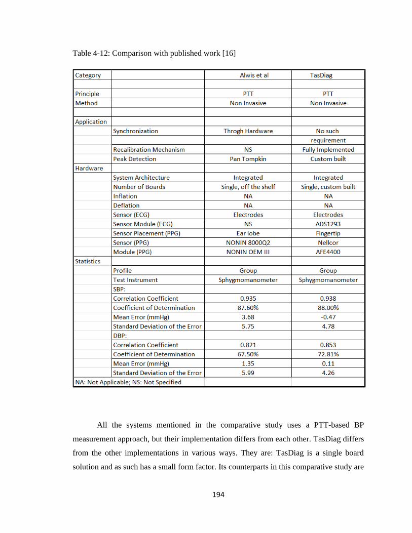
194
Table 4-12: Comparison with published work [16]
All the systems mentioned in the comparative study uses a PTT-based BP
measurement approach, but their implementation differs from each other. TasDiag differs
from the other implementations in various ways. They are: TasDiag is a single board
solution and as such has a small form factor. Its counterparts in this comparative study are

195
implemented using multi-boards, multi-processors and having a large form factor. This
architecture also warrants the synchronization problem among the boards. Secondly, the
PTT-based BP measurement needs a comprehensive recalibration maneuver. The systems
in the comparative study either ignored this important phenomenon or investigated very
little on this. In TasDiag, a comprehensive recalibration routine has been implemented in
its application. This is very unique compared to its counterparts. And finally, performance
analysis shows that TasDiag performs better than its counterparts in terms of mean error
and standard deviation. In the case of TasDiag, these important statistical parameters are
very much within the range stipulated by AAMI.

196
Chapter 5 : Conclusion and Future Work Scope
Biosignal monitoring and analysis are the backbones of diagnosis and treatment of
numerous medical conditions. Monitoring and analyzing biosignals along with other linear
health data have paramount importance to the health professionals and the concerned public
in general. The continuous and non‐invasive measurement of arterial blood pressure is a
major challenge in the medical monitoring field. In particular, there is a high demand from
clinicians and patients on new technologies allowing measuring cuff-less BP in ambulatory
care, compared to current techniques.
This PhD thesis has identified PTT based techniques to be a candidate approach to
respond to this demand. And has presented the implementation of a biosignal computing
platform (TasDiag) for calculating various health indices including blood pressure
continuously and non-invasively based on PTT. In doing so, this thesis has contributed to
the following:
By default, all the medical instrumentations, thus far, use the discrete analog front
end as its interface to the analog world. Being analog, signal processing is limited and thus
incurs errors, and needs constant calibration. This also demands computationally extensive,
time-consuming signal processing. This thesis implemented the interfacing circuitry with
highly integrated programmable AFEs, replacing the discrete analog front ends. This new
design paradigm paves the way to shift signal processing from the analog domain to the
digital domain and allows the designer to implement custom signal processing. As a result,
signal acquisition, and conditioning can be done under program control and with ease. This
implementation also reduces component count and overall power consumption.
PTT based BP measurement is based on the detection of features on the proximal
and distal waveforms in the central artery. For convenience, the ECG waveform is used as
the proximal and the PPG is used as the distal waveforms and the R-wave-to- peak time
delay is the PTT. Many effective R-wave detection methods are out there, with the most
popular being the Pan and Tompkins [168]. These methods are computationally intensive.
In this thesis, those methods are avoided and introduces customized detection method,
which is computationally less intensive and easy to implement.

197
The relationship between PTT and BP has been known to the scientific community
for long. While progress on PTT-based BP monitoring has been made, research is still
needed to best realize this approach. Using this approach, this thesis presents yet another
implementation (TasDiag) for cuff-less continuous BP measurements with promising
experimental results. The results comply with the AAMI standard.
It is expected that the PTT-based BP monitor should be non-invasive and
automated. Further, the form factor should be easier to use than a cuff. A single sensor unit
form factor would be ideal [10]. In that respect, TasDiag is a single board solution, yet a
multi-modal system capable of computing various health indices including BP in a
continuous and cuff-less manner. TasDiag has a physical form factor of 6 inches by 4
inches and can run on battery without interruption, an ideal time of 7.40 hours.
5.1. Conclusion
Having a medical instrumentation system, at significantly reduced size, power, and
capable of providing healthcare data remotely in a non-invasive and continuous way would
be a useful device at home to make our homes smarter and help achieve pervasive health
care system a reality.
A candidate technique to perform continuous and non‐invasive BP measurements
has been known since 1905. Commonly known as pulse wave velocity (PWV), this
technique exploits the fact that the velocity at which arterial pressure pulses propagate
along the arterial tree depends on the underlying BP. Hence, after a preliminary calibration
maneuver, one can obtain indirect measurements of BP by continuously measuring PWV
values on a given arterial segment. While some progress on PTT-based BP measurement
has been made, however, research is still needed to realize this approach in the best possible
way. There have been many technological and scientific developments in the recent past,
such as in sensor technology, computing, and smartphones that drives the research
community towards the best realization. For that, various computing models for bio-signals
are also emerging to compute various health indices including BP. The availability of

198
highly integrated analog sub-system front ends make developing medical instrumentation
possible today than before. This new development enables the designer to implement a
custom algorithm to implement those computing models for bio-signals and ushers new
design paradigms for system development, specifically, highly integrated AFE based
embedded systems for medical instrumentations. This research took advantage of all these
developments both in semiconductor technology and in alternative methods of biosignal
computing. The outcome is TasDiag; a biosignal computing platform for measuring
various health indices, such as BP, HR, SpO2, and body temperature in a non-invasive and
continuous manner.
For validation and performance measurements, long-term health data (sample
points) were collected from 30 subjects. Sample points were collected using TasDiag and
industry-standard clinical instruments. Collected sample points were subjected to various
statistical analyses. Validation and performance of TasDiag were done by setting criteria
in terms of mean, standard deviation, coefficient of correlation, mean absolute percentage
error, mean absolute error, mean difference, and standard deviation of the difference. The
rigorous analysis was also performed in terms of bias, scatter plot, Bland-Altman plot, and
histograms. In the case of the BP parameter, for SBP, the mean differences in readings
between TasDiag and Omron are -0.47 mmHg and a standard deviation of difference is
4.78 mmHg. For DBP, the mean difference is 0.11 mmHg and the standard deviation is
4.26 mmHg. In both cases, the mean difference and standard deviation comply with the
AAMI standard. According to AAMI, the mean difference must be less than ±5 mmHg and
the standard deviation must be less than 8 mmHg. The correlation coefficient between the
readings (Omron vs TasDiag) is 0.938 for SBP and 0.853 for DBP, which are statistically
very significant. TasDiag is also tested using a single profile, whereby, long-term sample
points were collected from a single subject using TasDiag and Omron BP meter. In that,
for SBP, the mean differences in readings between TasDiag and Omron are -0.31 mmHg
and a standard deviation of difference is 3.48 mmHg. In the case of DBP, the mean
difference is 0.28 mmHg and the standard deviation is 2.79 mmHg. Again, the mean
difference and the standard deviation both lie within the specification outlined by AAMI.
In the single profile, the correlation coefficient between the readings (Omron vs TasDiag)
is 0.947 for SBP and 0.856 for DBP, which are statistically very significant. From the

199
statistical analysis, it is also found that in both cases (SBP and DBP), in 95% cases, the
difference in readings lie within the limit of agreement, which is within the confidence
interval. For the HR parameter, the mean difference in readings between TasDiag and
Omron/Datex is -0.21 bpm and the standard deviation of difference is 0.95 bpm. In the case
of SpO2, the mean difference in readings between TasDiag and Datex patient monitor is -
0.46-percentage point and the standard deviation of difference is 0.97 percentage point.
For body temperature, the mean difference in readings between TasDiag and Veridian
thermometer is 0.15 0F and the standard deviation of difference is 0.26 0F. For all these
parameters, such as HR, SpO2, and body temperature, the mean differences and standard
deviations all lie less than one point. That tells us that TasDiag can easily replace its
counterparts. Based on the correlation measurements, as described in the results chapter,
the results find a significant correlation between the readings by TasDiag and that of its
counterparts. Test results also indicate high agreement and reliability between TasDiag and
standard instruments in all cases of health indices.
TasDiag is also compared with other implementations proposed by other
researchers for comparative study. The comparative study reveals that the proposed
systems are based on multi- boards compared to TasDiag, which is a single board solution.
The comparative study also shows the statistical test results for performance and accuracy.
In statistical parameters, TasDiag performs better or very competitive to those mentioned
in the comparative studies. PWV‐based approach to assess BP requires a constant
calibration maneuver to identify a subject‐dependent mapping of the measured PTT values
towards the underlying BP values. TasDiag has a unique approach to handle this issue as
described in section 3.1.1, 3.1.2, and section 3.1.3, while the other implementations did not
investigate it at all [143]. Besides, TasDiag is a multi-modal system. TasDiag is integrated
yet open for future expansion. For expansion, we need an SPI compatible AFE and add a
software module to operate that AFE. That is add up exercise to the original design. In that
way, it is an open computing platform and open to future expansion.
Like any other model, PTT based BP measurement has its limitations too. Pulse
transit time is related to the elasticity of the arterial wall. With age and medical conditions,
the elasticity of the arterial wall changes and thus PTT based BP models necessitate
recalibration. Also, there is a mismatch between the theory and practice of PTT-based BP

200
measurement. In theory, PTT is measured through central arteries via the foot-to-foot time
delay between proximal and distal waveforms. However, for convenience, ECG is
employed as a proximal waveform and PPG as a distal waveform. The time delay between
R-wave-to-peak between these waveforms is the pulse arrival time (PAT). The resulting
PAT estimates through peripheral arteries correlate well with SBP, rather than DBP [10].
This was also the case in TasDiag.
In conclusion, this thesis showed that there exist technological solutions for the
continuous, cuff-less measurement of BP in ambulatory settings. In particular, PTT based
BP measurement is highlighted as a potential candidate that might fulfill the demand of the
health professionals and general mass for a BP monitoring device that is non-invasive,
unsupervised, accurate, and continuous. Also suitable for ubiquitous monitoring and can
be used in ambulatory. The results presented in this thesis might help to transform our
present hospital-based health care system to home-based one.
5.2 Future Scope
The thesis research path consisted of an initial theoretical exploration of the field,
followed by the identification of potential solutions and their experimental implementation.
Along this path, several crossroads were encountered for which decision and trade‐offs
were made. In the following, the limitations of the performed research work are provided
together with suggestions on possible tracks to be followed in the future.
PWV- based technology was selected as the optimal solution because of its strictly
non‐invasive nature, and because of the existence of a theoretical model supporting its
validity. Therefore, from this decision point, the entire thesis research work was tailored
towards the development of a biosignal computing platform based on the PTT concept,
discarding other approaches. The ECG waveform was employed as a surrogate of the
proximal waveform. It is convenient, robust against artifacts, and enables tracking systolic
BP. However, this waveform introduces the pulse ejaculation period (PEP), which could a
major confounding factor that necessitates frequent recalibration. [169]. By contrast,

201
Impedance Cardiography (ICG) can measure an actual proximal waveform. Thus can be
used in future endeavor.
To enhance accuracy, research is sorely needed to improve the calibration of PTT
to BP. For that, a single cuff BP measurement could be obtained from the subject every so
often. The collection of training sample points comprising pairs of PTT estimates and BP
values during a set of BP varying interventions per subject from a vast number of diverse
subjects is necessary. Collecting the training data is a serious endeavor but the best way to
popularize the PTT based BP monitoring.
Further work is also needed to estimate SBP and DBP independently. A single PTT
estimation cannot indicate these two BP values when they are not varying in the same
direction (e.g., isolated systolic hypertension) [10]. For that, models are incorporating
simple covariates, such as heart rate, and height [16] [65] [143] [144]. In the future, of
particular interest would be to explore those models based on the prediction of BP by the
multi‐parametric processing of cardiovascular and physical variables.
Efforts to measure BP based on Pulse Wave Velocity is going on for quite some
time now. On the one side, clinically‐validated technologies have been developed to
measure PWV of central arteries non‐invasively but they are not adapted to ambulatory
uses. TasDiag is an ambulatory solution. As such, more clinical assessment is to be
performed: an additional large population experimental campaign is required to assess the
accuracy of TasDiag on tracking continuous BP changes for each subject. It will be a
fruitful endeavor to calibrate TasDiag against the catheterization method. The
catheterization method though pervasive but the gold standard method for accurate BP
measurement.
Considering the present hardware of TasDiag, it would be useful to add a graphic
display instead of the present liquid crystal display, which is alphanumeric. The graphic
display would allow displaying biosignals, such as ECG on it. The present temperature
interface should be replaced by a non-contact infrared-based temperature sensor. Taking
the open architecture concept of TasDiag, in the future, more AFEs specific to EEG, EKG,
and blood sugar can be added. It would be an interesting future endeavor to implement
TasDiag as a system on a chip (SoC) to further reduce component count and thus help
reduce the overall size and power consumption. And will make TasDiag a sought after

202
addition to manned space missions as suggested in [25], and to a data acquisition system,
as proposed in [26].
TasDiag is capable of sharing medical data with remote devices. As proof of
concept, an android-based application has been developed in this thesis and data was shared
with an android smartphone. Considering the nature of data (privacy and security),
cryptography should be adopted in the application. In the present thesis, cryptography was
not investigated. The future endeavor should include this feature.

203
Appendix A. Tables and Figures
Validation Sample Points: The sample points are to be read from top to bottom and left
to right. The sample points before the number 85 represent the maxima in the cycles.
Table A-1: Validation Sample Points for ECG Peak Detection

204

205

206
Table A-2: Validation Sample Points for PPG Peak Detection

207

208

209

210
Table A-3: BP-PTT Sample Points (Group)

211

212

213

214

215

216
Table A-4: BP Readings (Omron vs TasDiag: Group)

217

218

219

220
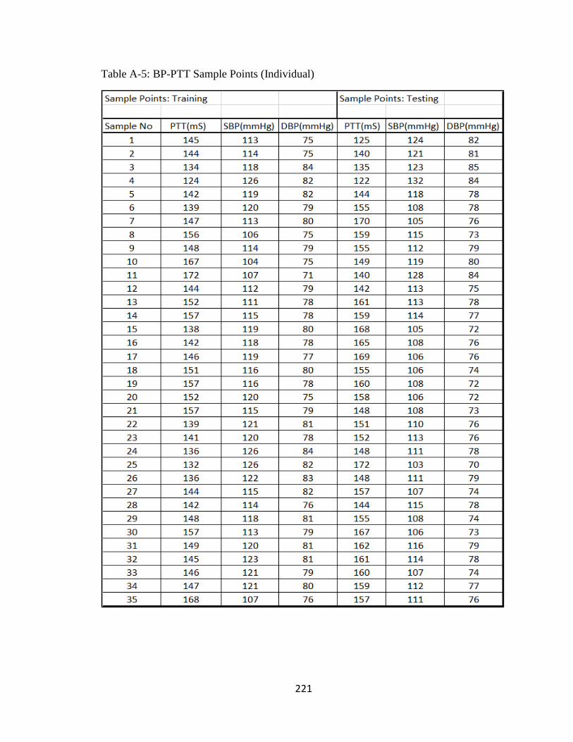
221
Table A-5: BP-PTT Sample Points (Individual)

222

223

224

225
Table A-6: BP Readings (Omron vs TasDiag: Individual)

226

227

228
Table A-7: Heart Rate Readings (Datex/Omron vs TasDiag)
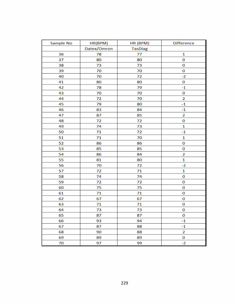
229

230

231

232
Table A-8: SpO2 Readings (Datex vs TasDiag)
Sample No SPO2 (%) SPO2 (%) Difference
Datex TasDiag
1 95 95 0
2 94 96 -2
3 95 97 -2
4 97 97 0
5 96 97 -1
6 97 96 1
7 97 97 0
8 97 98 -1
9 97 97 0
10 97 97 0
11 96 96 0
12 96 96 0
13 96 97 -1
14 95 95 0
15 95 95 0
16 96 96 0
17 98 99 -1
18 97 97 0
19 97 99 -2
20 97 98 -1
21 97 98 -1
22 98 99 -1
23 97 99 -2
24 97 99 -2
25 99 99 0
26 97 99 -2
27 98 99 -1
28 98 98 0
29 98 98 0
30 97 96 1
31 98 97 1
32 97 96 1
33 97 98 -1
34 98 96 2
35 96 96 0

233

234

235

236
Table A-9: Temperature Readings (Veridian vs TasDiag)

237

238
Figure A-1: MCU Schematic Sheet

239
Figure A-2: ECG Schematic Sheet

240
Figure A-3: PPG Schematic Sheet

241
Figure A-4: Temperature Schematic Sheet

242
Figure A-5: Communication Schematic Sheet

243
Figure A-6: Power Schematic Sheet

244
References
[1] M. S. Rahman, "Health care in aged population, New Age," 23 January 2019.
[Online]. Available: http://www.newagebd.net/print/article/62671. [Accessed 23
January 2019].
[2] H. Medjahed, J. B. Dan Istrate, Bernadette and B. Dorizzi, "Human activities of
daily living recognition using fuzzy logic for elderly home monitoring," in FUZZ-
IEEE 2009, IEEE International Conference on Fuzzy Systems, Jeju Island, S. Korea,
2009.
[3] M. a. T.M.Gatton, "Fuzzy Logic Desicion Making for an Intelligent Home
Healthcare System.," in 5th International Conference on Future Information
Technology, 2010.
[4] S. C. a. o. o. t. S. o. F. Institution, "Action for Seniors," Government of Canada, Fall
2014.
[5] N. J. A. a. J. Ahn, "Gastro Sanitario Y Enve Je Ci miento de la poblacion en
Espania," Foundacion BBVA, Documento de Trabajo, 7, 2003.
[6] S. Zwweifel, "Ageing population and Health Care Expenditure: A Red Herring?,"
Health Economics, pp. 485-496, 1999.
[7] Koopmanschap, M., Meijer, C. de, Polder and a. Johan, "Determinants of
Healthcare Expenditure in an aging society," Netspar panel papers, p. 22, 2010.
[8] D. o. H. S. a. Informatics, "Causes of death 2008: data sources and methods,"
World Health Organization, Geneva, 2011.
[9] W. H. Organization, "A global brief on hypertension: Silent killer, global public
health crisis," Geneva, 2013.
[10] J.-O. H. O. T. I. L. K. M. C.-S. K. H. T. a. S. K. Ramakrishna Mukkamala, "Toward
Ubiquitous Blood Pressure Monitoring via Pulse Transit Time: Theory and

245
Practice," IEEE Transactions on Biomedical Engineering, vol. 62, no. 8, pp. 1879-
1901, 2015.
[11] K. Soundarapandian and M. Berarducci, "Analog Front-End Design for ECG
Systems using Delta-Sigma ADCs," Texas Instruments, 2009-2010.
[12] D. P. Sametriya and N. M. Vasavada, "HC-CPSoC: Hybrid Cluster NoC Topology for
CPSoC," in IEEE WISPNET Conference, 2016.
[13] N. M. Vasavada, D. P. Sametriya and D. S. Vasava, "Power Efficient
Implementation of MVA-SI on Speech Controlled IoT System," in IEEE
International Conference on Recent Trends In Electronics Information
Communication Technology, 2016.
[14] S. Sarma, N. Dutt, P. Gupta, N. Venkatassubramanian and A. Nicolau,
"CyberPhysical-System on Chip (CPSoC): A self-Aware MPSoC Paradigm with Cross
Layer Virtual Sensing and Actuation," in Design, Automation & Test in Europe
Conference & Exhibition, 2015.
[15] K. K. Kim, W. Wang and K. Choi, "On-Chip Aging Sensor Circuits for Reliable
Nanometer MOSFET Digital Circuits," IEEE Transactions on Circuits and Systems II:
Express Briefs, vol. 57, no. 10, pp. 798-802, 2010.
[16] W. D. Alwis, R. Rajapaksha, N. Ranaweera, P. Pitigalaarachchi and A.Pasqual,
"Parametric Model between Pulse Transit Time and Systolic and Diastolic Blood
Pressures for Non-Invasive Blood Pressure Estimation," in IEEE Conference on
Biomedical Engineering and Sciences(IECBES), 2014.
[17] W. MY, P. CC and Z. YT, "An evaluation of the cuffless blood pressure estimation
based on pulse transit time technique: A half year study on normotensive
subjects," Cardiovascular Engineering, vol. 9, pp. 32-38, 2009.
[18] W. Chen, T. Kobayashi, S. Ichikawa, Y. Takeuchi and T. Tagawa, "Continuous
estimation of systolic blood pressure using the pulse arrival time and intermittent
calibration," Medical and Biological Engineering and Computing, vol. 38, pp. 569-
574, 2000.

246
[19] Y. S. Yan and Y. T. Zhang, "A novel calibration method for noninvasive blood
pressure measurement using pulse transit time," in 4th IEEE/EMBS International
summer school and symposium on Medical devices and biosensors, Cambridge,
UK, 2007.
[20] Y. Y, C. JH and Y. G, "Non-constrained blood pressure monitoring using ECG and
PPG for personal healthcare," Journal of Medical Systems, vol. 33, pp. 261-266,
2009.
[21] B. a. A. M. B.M. McCarthy, "An investigation of pulse transit time as a non-
invasive blood pressure measurement method," in Journal of Physics: Conference
Series, Volume 307, Number 1, 2011.
[22] J. M. S. I. Caros, Continuous non-invasive blood pressure estimation, Zurich,
Switzerland: Swiss Federal Instirute of Technoloy (ETH), 2011.
[23] S. DH, B. Z and B. WC, "The smart house for older persons and persons with
disabilities: structure, technology arrangements, and perspectives," IEEE
Transsactions on Neural Systems and Rehabilitation Engineering, vol. 12, no. 2,
pp. 228-250, 2004.
[24] J. Muthuswamy, "Biomedical Signal Analysis," in Standard Handbook of
Biomedical Engineering and Design, McGraw-Hill, 2004, p. Chapter 18.
[25] J. M. Eklund and N. Khan, "A bio-signal computing platform for real-time online
health analytics for manned space missions," in IEEE Aerospace Conference,
Montana, USA, 2018.
[26] N. Khan and J. M. Eklund, "A highly Integrated Computing Platform for
continuous, non-invasive BP estimation," in IEEE Canadian Conference on
Electrical and Computer Engineering (CCECE), Quebec, Canada, 2018.
[27] Wikipedia, "Signal Processing," 11 June 2019. [Online]. Available:
https://en.wikipedia.org/wiki/signal processing. [Accessed 15 June 2019].
[28] J. Webster, The origin of Biopotentials in Medical Instrumentation Application
and Design, Wiley, 4th Edition, 2009.

247
[29] K. K. M. Rahman and M. Nasor, "Multipurpose low cost bio-daq system for real
time biomedical applications," in International conference on Information and
communication Technology Research (ICTRC), 2015.
[30] E. Stein, Rapid Analysis of Electrocardiogram - A self study Program, Lippincott &
Wilkins, 3rd Edition, 2000.
[31] J.G.Webster, The origin of Biopotentials in Medical Instrumentation Application
and Design, Wiley, 4th Edition, 2009.
[32] R. P. J. Malmivuo, "The Heart", Bioelectromagnetism principles and Applications
of Bioelectric and Biomagnetic Fields, New York: Oxford university Press, 1995.
[33] J. Guerreiro, "A Biodignal Embedded System for Physiological Computing,"
Instituto Superior de Engenharia de Lisboa, Lisbon, Portugal, 2013.
[34] F. Agrafioti, "ECG in Biometric Recognition: Time Dependency and Application
Challenges," Dept. of Electrical and Computer Engineering, University of Toronto,
Toronto, 2011.
[35] L. S. a. P. Laguna, Bioelectrical Signal Processing in Cardiac and Neurological
Applications, vol. 17, Elsevier, 2005, pp. 261-271.
[36] V.J.Kumar and V.Blazek, "Photoplethsymography for non-invasive diagnostics," in
Smart Instrumentation, Measurement and Applications(ICSIMA), IEEE,
Kualalumpur, 2013.
[37] R. Banerjee, A.Sinha, A.Pal and A.Kumar, "Estimation of ECG parameters using
photoplethysmography," in 13th International Conference on BioInformatics and
BioEngineering, 2013.
[38] S.-J. Jung, Y.-D. Lee, Y.-S. Seo and W.-Y. Chung, "Design of a low-power
consumption wearable reflectance pulse oximetry for ubiquitous healthcare
system," in International conference on Control, Automation and System , 2008.

248
[39] T. Tamura, Y. Maeda, M. Sekine and M. Yoshida, "Wearable
Photoplethysmographic Sensors - Past and Present," Electronics, vol. 3, pp. 282-
302, 2014.
[40] S.-S. Oak and P. Aroul, "How to Design Peripheral Oxygen Saturation (SPO2) and
Optical Heart Rate Monitoring (OHRM) Systems Using the AFE4403," Texas
Instruments, 2015.
[41] Y.Mendelson, "Pulse oximetry: theory and applications for noninvasive
monitoring," Clin. Chem, vol. 38, no. 9, pp. 1601-1607, 1992.
[42] M. Wukitsch, M.T.Petterson, D.R.Tobler and J.A.Polong, "Pulse oximetry: Analysis
of theory, technology, and practice," J. Clin. Monit., vol. 4, no. 4, pp. 290-301,
1988.
[43] J.P.Decock and L.Tarassenko, "Pulse oximetry: Theoretical and experimental
models," Med. Biol. Eng. Comput., vol. 17, no. 1, pp. 291-300, 1993.
[44] W.J.Tompkins, Biomedical Digital Signal Processing, Prentice Hall, 2000.
[45] R. AA, "Thermoregulation: Some concepts have changed. Fuctional architecture
of the thermoregulatory system.," Americal journal of physiology,
Regulatory,Integrative, and Comparative physiology, vol. 292, no. 1, pp. 37-46,
2007.
[46] P. Oguz and G. Ertas, "Wireless dual channel human body temperature
measurement device," in International Conference on Electronics, Computer and
Computation(ICECCO), 2013.
[47] D. Semiconductor, "DS18B20, 1-Wire Digital Thermometer," www.dalsemi.com.
[48] P. Narczyk, K. Siwiec and W. A. Pleskacz, "Analog front-end for precise human
body temperature measurement," in IEEE 20th International Symposium on
Design and Diagnostics of Electronic Circuits & Systems(DDECS), 2017.

249
[49] P. Narczyk, K. Siwiec and W. A. Pleskacz, "Precision human body temperature
measurement based on thermistor," in IEEE 19th International Symposium on
Design and Diagnostics of Electronic Circuits & Systems(DDECS), 2016.
[50] W. Haines, P. Momenroodaki, E. Berry, M. Fromandi and Z. Popvic, "Wireless
system for continous monitoring of core body temperature," in IEEE MTT-S
International Microwave Symposium (IMS), 2017.
[51] H. Liu, H. Jiang, K. Yang, Z. Chi, F. Li, C. Zhang and Z. Wang, "A fully integrated
wireless SoC in-body pH and temperature continuous monitoring," in
International SoC Design Conference (ISOCC), 2015.
[52] M. Rao, T. Newe, I. Grout, E. Lewis and A. Mathus, "FPGA Based Real Time secure
Body Temperature Monitoring suitable for WBSN," in IEEE International
Conference on Computer and Information Technology, 2015.
[53] C. A. Boano, M. Lasagni and K. Romer, "Non-invasive measurement of core body
temperature in Marathon runners," in IEEE International Conference on Body
Sensor Networks., 2013.
[54] Y. Chen, H. Zhang and N. Wang, "Body temperature Monitor and Alarm system
used in Hospital Based on 1-wire and wireless communication Technology," in
International workshop on Geoscience and Remote sensing, 2008.
[55] T. H. Y. Ling and L. J. Wong, "Elderly infrered body temperature telemonitoring
system with XBEE wireless protocol.," in 9th International Conference on Sensing
Technology (ICST), 2015.
[56] P.-W. Huang, T.-H. Chang, M.-J. Lee, T.-M. Lin and Meng-Liang, "An Embedded
Non-Contact Body Temperature Measurement System with Automatic Face
Tracking and Neural Network Regression," in International Automatic Control
Conference (CACS), 2016.
[57] H.-F. Tang and K. Hung, "Design of a non-contact body temperature
measurement system for smart campus," in IEEE International Conference on
Consumer Electronics-China (ICCE-China), 2016.

250
[58] L. Ercoli, P. Marchionni, L. Scalise, E. P. Tomasini and V. P. Carnielli, "Non contact
measurement of body temperature for the identification of thermoregulation
abilities in preterm patients," in Sensors, 2013 IEEE, 2013.
[59] A.V.Osadchuk, A.A.Semennov, S. Baraban, E. Semenova and K.O.Koval,
"Noncontact infrared thermometer based on a self-oscillating lambda type
system for measuring human body's temperature," in 23rd IEEE International
Crimean Conference "Microwave 7 Telecommunication Technology", 2013.
[60] e. a. N. Westerhof, Snapshots of Hemodynamics, Springer, 2005.
[61] H. Gesche, D. GrossKurth, G. Kiichler and A. Patzak, "Continuous blood pressure
measurement by using the pulse transit time: comparison to a cuff-based
method," European Journal of Applied physiology, vol. 112, 2011.
[62] S. S. Shahrbabaki, B. Ahmed, T. Penzel and D. Cvetkovic, "Blood pressure and
cardiovascular parameters during sleep arousals," in 39th Annual International
Conference of the IEEE Engineering in Medicine and Biology Society(EMBC), 2017.
[63] P. Fung, G. Dumont, C. Ries, C. Mott and M. Ansermino, "Continuous Noninvasive
Blood Pressure Measurement by Pulse Transit Time," in 26th Annual International
Conference of the IEEE EMBS, San Francisco, CA, USA, 2004.
[64] X.F.Teng and Y.T.Zhang, "Continuous and Noninvasive Estimation of Arterial
Blood Pressure Using a Photoolethysmographic Approach," in 25th Annual
International Conference of the IEEE EMBS, Cancun, Mexico, 2004.
[65] S.-y. Ye, G.-R. Kim, D.-K. Jung, S.-w. Baik and G.-r. Jeon, "Estimation of Systolic and
Diastolic Pressure using the Pulse Transit Time," International journal of Medical,
Health, Biomedical, Bioengineering and Pharmaceutical Engineering, vol. 4, no. 7,
pp. 303-308, 2010.
[66] S. A and E. J. Jothi, "Pulse Transit Time Measurement Using ATmega16
Microcontroller," International Journal of Advanced Research in Computer
Science and Software Engineering, vol. 3, no. 3, pp. 688-691, 2013.

251
[67] C.C.Y.Poon and Y.T.Zhang, "Cuff-less and Noninvasive Measurements of Arterial
Blood Pressure by Pulse Transit Time," in Engineering in Medicine and Biology
27th Annual Conference, Shanghai, China, 2005.
[68] S. N. Bose and C. Kumar, "Improving the Performance of Continuous Non-invasive
Estimation of Blood Pressure Using ECG and PPG," in IEEE INDICON, 2015.
[69] X.-R. Ding, Y.-T. Zhang, J. Liu, W.-X. Dai and H. K. Tsang, "Continuous Cuffless
Blood Pressure Estimation Using Pulse Transit Time and Photoplethysmogram
Intensisty Ratio," IEEE Transactions on Biomedical Engineering, vol. 63, no. 5, pp.
964-972, 2016.
[70] E.K.Park, B.H.Cho, S.H.Park, J.Y.Lee, J.S.Lee, I.Y.Kim and Sun.I.Kim, "Continuous
measurement of systolic blood pressure using the PTT and other parameters," in
Engineering in Medicine and Biology 27th Annual Conference, Shanghai, China,
2005.
[71] J.M.Zhang, P.F.Wei and Y.Li, "A LabVIEW Based Measure System for Pulse Wave
Transit Time," in 5th International Conference on Information Technology and
Application in Biomedicine, Shenzhen, China, 2008.
[72] S. Ghosh, A. Banerjee, N. Ray, P. W. Wood, P. Boulanger and R. Padwal,
"Continuous blood pressure prediction from pulse transit time using ECG and PPG
signals," in IEEE Healthcare Innovation Point-Of-Care Technologies Conference(HI-
POCT), 2016.
[73] R. Wang, W. Jia, Z.-H. Mao, R. J. Sclabassi and M. Sun, "Cuff_free blood pressure
estimation using pulse transit time and heart rate," in 12th International
Conference on Signal Processing(ICSP), 2014.
[74] X.F.Feng and Y.T.Zhang, "An Evaluation of a PTT-Based Method for Noninvasive
and cuffless Estimation of Arterial Blood Pressure," in International Conference of
the IEEE Engineering in Medicine and Biology Society, New York City, USA, 2006.
[75] W.-H. Lin, H. Wang, O. W. Samuel and G. Li, "Using a new PPG indicator to
increase the accuracy of PTT-based continuous cuffless blodd pressure

252
estimation," in 39th Annual International Conference of the IEEE Engineering in
Medicine and Biology Society(EMBC), 2017.
[76] X.-R. Ding and Y.-T. Zhang, "Photoplethysmogram intensity ratio: A potential
indicator for improving the accuracy of PTT-based cuffless blood pressure
estimation," in 37th Annual International Conference of the IEEE Engineering in
Medicine and Biology Society(EMBC), 2015.
[77] X.-R. Ding, Y.-T. Zhang and H. K. Tsang, "Anew modeling methodology for
continuous cuffless blood pressure measurement," in IEEE-EMBS International
Conference on Biomedical and Health informatics(BHI), 2016.
[78] P. CC and Z. YT, "Cuff-less and noninvasive measurements of arterial blood
pressure by pulse transit time," in 27th Annual International Conference of the
IEEE Engineering in Medicine and Biology Society, 2005.
[79] C. Y, W. C, T. G, B. M and L. G, "Continuous and noninvasive blood pressure
measurement: A novel modeling methodology of the relationship between blood
pressure and pulse wave velocity," Annuals Biomedical Engineering, vol. 37, pp.
2222-2233, 2009.
[80] M. Rourke, J.A.Staessen, C. Vlachopoulos, D.Duprez and a. G. Plante, "Clinical
Applications of Arterial Stiffness; Definitions and Reference Values," American
Journal of Hypertension, vol. 15, pp. 426-444, 2002.
[81] D.J.Hughes, C.F.Babbs, L.A.Geddes and J.D.Bourland, "Measurement of Young's
modulus of elasticity of the canine aorta with ultrasound," Ultrasonic Imaging,
vol. 1, pp. 356-367, 1979.
[82] e. a. E. O'Brien, "Blood Pressure Measuring Devices: recommendations of the
European society of Hypertension," BMJ, vol. 322, pp. 531-6, 2001.
[83] J.G.Webster, Biopotential Electrodes: Mechanical Instrumentation- Application
and Design, Wiely, 4th Edition, 2009.

253
[84] A. B. a. M. J. Burke, "Measurement of the electrical properties of ungelled ecg
electrodes," International journal of Biology and Biomedical Engineering, vol. 2,
no. 3, pp. 89-97, 2008.
[85] C. Networks.org, "en.ecgpedia.org," 12 05 2012. [Online]. Available:
http://www.wikidoc.org/index.php; File: De-Noise move.png. [Accessed 11 12
2019].
[86] J.G.Webster, "Basic concepts of Medical Instrumentation," in Medical
Instrumentation Application and Design, Wiley, 4th Edition, 2009.
[87] E. J. Woo, "Biomedical Instrumentation," in BME302, Dept. of Biomed.Eng.,
http://ejwoo.com.
[88] Husn-Hsien and J. M.F.Moura, "Introduction," in Biomedical Signal Processing,
McGraw Hill, 2010, pp. 559-579.
[89] J. G. T. B. a. G. C. 0. Majdalawieh, "Biomedical Signal Processing and
Rehabilitation Engineering: A review," in IEEE Pacific Rim Conference on
Communication and Signal Processing, Victoria, Canada, 2003.
[90] G. M. R. I. I. D. I. C. a. I. D. C. Levkov, "Removal of Power-line Interference from
the ECG: A review of the subtraction procedure," Biomedical Engineering Online,
vol. 4, pp. 1-8, 2005.
[91] E. L. M. a. R. M. E. A. Clancy, "Sampling, noise-reduction and amplitude
estimation issues in surface electromyography," Journal of Electromyography and
Kinesiology, vol. 12, pp. 1-16, 2002.
[92] P. L. P. I. P. J. K. C. e. a. G. Bonmassar, "Motion and ballistocardiagram artifact
removal for interleaved recording of EEG and EPs during MRI," Neuroimage, vol.
16, pp. 1127-1141, 2002.
[93] a. M. R. A.-S. S. Charleston, "Reduced order Kalman filtering for the enhancement
of respiratory sounds," in IEEE transactions on Biomedical Engineering, 1996.

254
[94] M. Atef, L. Xiyan, G. Wang and Y. Lian, "PTT Based Continuous Non-invasive Blood
Pressure System," in IEEE 59th International Midwest Symposium on Circuits and
Systems(MWSCAS), Abu Dhavi, UAE, 2016.
[95] D. L. Gaikwad and P. Kasliwal, "FPGA Based Critical Patient Health Monitoring
Using Fuzzy Neural Network," International Journal of Scientific & Engineering
Research, vol. 4, no. 3, pp. 1-5, 2013.
[96] R. A. Ramlee, M. A. B. Othman, M. I. B. A. Aziz and H. A. b. Sulaiman, "Low cost
Heart Rate Monitoring Device using Bluetooth," in IEEE 2nd International
Conference on Information and Communication Technology(ICoICT), 2014.
[97] S. Sali and D. C.S., "Integrated Wireless Instrument for Heart rate and Body
Temperature Measurement," in IEEE 2nd International Conference for
Convergence in Technology (I2CT), 2017.
[98] M. O'Donnel, "Biomedical Instrumentation & Design," in BME/EECS 458,
https://bme.umich.edu, 2016.
[99] B. G. John L. Semmlow, Biosignal and Medical Image, Newyork: CRC Press, 2014.
[100] K. Cai and X. Liang, "Development of Remote Monitoring Cardiac System Based
on GPRS," in IEEE International Conference on Biomedical Engineering and
Computer Science, 2010.
[101] K. Cai and X. Liang, "International Conference on Biomedical Engineering and
Computer Science," in IEEE Conferences, 2010.
[102] R.-G. Lee, K.-C. Chen, C.-C. Hsiaso and C.-L. Tseng, "A Mobile Care System With
Alert Mechanism," IEEE Transactions on Information Technology in Biomedicine,
vol. 11, no. 5, pp. 507-517, 2007.
[103] G. Fortino and V. Giampa, "PPG-Based methods for non invasive and continuous
blood pressure measurement: An overview and development issues in body
sensor networks," in IEEE International Workshop on Medical Measurements and
Applications, 2010.
255
[104] H. Alemzadeh and e. al, "An embedded reconfigurable architecture for patient -
specific multi-parameter medical monitoring," in Annual International conference
of the IEEE Engineering in Medicine and Biology society, Boston, Massachusetts,
USA, 2011.
[105] Y. Yang, X. Huang and X. Yu, "Real-Time ECG monitoring System Based on FPGA,"
in IECON 2007 - 33rd Annual Conference of the IEEE industrial Electronics Society,
Taipei, Taiwan, 2007.
[106] D. H. Gawali and V. M. Wadhai, "Mixed signal SoC based Bio-Sensor Node for long
term health monitoring," in IEEE International WIE Conference on Electrical and
Computer Engineering(WIECON-ECE)., 2016.
[107] F. Naaz and N. S. Grewal, "An SoC based wearable system for continuous Blood
Pressure measurement," in IEEE International conference on signal processing
and communication(ICSC), 2016.
[108] Z. Li, G. Feng, F. Liu, J. Q. Dong, R. Kamoua and W. Tang, "Wireless health
monitoring system," in IEEE Long Island Systems, Application and Technology
Conference, 2010.
[109] Chin-Teng, kuan-Cheng, Chun-Lin, Chia-Chiang, S.-W. Lu, S.-S. Chang, B.-S. Lin, H.-
Y. Liang, R.-J. Chen, Y.-T. Lee and L.-W. Ko, "An Intelligent Telecardiology System
Using a Wearable and Wireless ECG to detect Artial Fibrillation," IEEE
Transactions on Information Technology in Biomedicine, vol. 14, no. 3, pp. 726-
733, 2010.
[110] Y. Jang, H. W. Noh, I.B.Lee, J.-W. Jung, Y. Song, S. Lee and S. Kim, "Development
of a patch type embedded cardiac function monitoring system using dual
microprocessor for arrhythmia detection in heart disease patient," in Annual
International Conference of the IEEE Engineering in Medicine and Biology Society,
San Diego, California USA, 2012.

256
[111] M. M. Islam, F. H. M. Rafi, M. Ahmad and A. F. Mitul, "Microcontroller based
health care system using sensor network," in 7th International Conference on
Electrical and Computer Engineering, Dhaka, Bangladesh, 2012.
[112] C. D. Capua, A. Meduri and R. Morello, "A remote doctor for homecare and
medical diagnoses on cardiac patients by an adaptive ECG analysis," in IEEE
International Workshop on Medical Measurements and Applications, Cetraro,
Italy, 2009.
[113] V. Srovnal and M. Penhaker, "Health Maintenance Embedded Systems in Home
Care Applications," in Second International Conference on Systems(ICONS'07),
2007.
[114] M. Atef, L. Xiyan, G. Wang and Y. Lian, "PTT Based Continuous Time Non-invasive
Blood Pressure System," in IEEE 59th International Midwest Symposium on
Circuits and Systems (MWSCAS), Abu Dhabi, UAE, 2016.
[115] Y. Zheng, B. P. Yan, Y. Zhang, C.M.Yu and C. C.Y.Poon, "Wearable Cuff-less PTT-
based System for overnight Blood Pressure Monitoring," in 35th Annual
International Conference of the IEEE EMBS, Osaka, Japan, 2013.
[116] S. Sali and P. C.S, "Integrated Wireless Instrument for Heart rate and Body
temperature measurement," in 2nd International Conference for Convergence in
Technology, 2017.
[117] S. K. Nayak, D. Biswal, B.Champaty, A. Anis, B. Mohapatra and D. N. Tibarewala,
"Development of a simultaneous acquisition system for ECG, PCG and body
temperature signals.," in Annual IEEE India Conference(INDICON), 2015.
[118] A. A. Aboughaly, D. Iqbal, M. A. E. Ghany and K. Hofman, "NICBPM: Non-invasive
cuff-less blood pressure monitor," in 29th International conference on
Microelectronics (ICM), 2017.
[119] A. Esmaili, M. Kachuee and M. Shabany, "Nonlinear Cuffless Blood Pressure
Estimation of Healthy Subjects Using Pulse Transit Time and Arrival Time," IEEE

257
Transactions on Instrumentation and Measurement, vol. 66, no. 12, pp. 3299-
3308, 2017.
[120] C.-C. Hsiao, H.-C. Kuo, R.-G. Lee and R. Lin, "Effects of pulse transit time and
physiological differences on wearable device based blood pressure estimation,"
in International Automatic Control Conference (CACS), Taichung, Taiwan, 2016.
[121] M. Singh and N. Jain, "Performance and Evaluation of Smartphone Based
Wireless Blood Pressure Monitoring System Using Bluetooth," IEEE Sensors
Journal, vol. 16, no. 23, pp. 8322-8328, 2016.
[122] D. Buxi, J.-M. Redute and M. R. Yuce, "Blood Pressure Estimation Using Pulse
Transit Time From Bioimpedance and Continuous Wave Radar," IEEE Transactions
on Biomedical Engineering, vol. 64, no. 4, pp. 917-927, 2017.
[123] X.-R. Ding, Y.-T. Zhang, J. Liu, W.-X. Dai and H. K. Tsang, "Continous Cuffless Blodd
Pressure Estimation Using Pulse Transit Time and Photoplethysmogram Intensity
Ratio," IEEE Transactions on Biomedical Engineering, vol. 63, no. 5, pp. 964-972,
2016.
[124] N. K. A, L. K. Vincent, L. Varghese, L. V.L, N. J. A and Y. C.V, "Wireless Health
Monitoring System for ECG, EMG and EEG Detecting," in International Conference
on Innovations in Information, Embedded and Communication Systems (ICIIECS),
2017.
[125] M. S. Mahmud, H. Wang, A. M. Esfar-E-Alam and H. Fang, "A wireless Health
Monitoring System Using Mobile Phone Accessories," IEEE Internet of Things
Journal, vol. 4, no. 6, pp. 2009-2018, 2017.
[126] P.-W. Huang, C.-H. Lin, M.-L. Chung, T.-M. Lin and B.-F. Wu, "Image based
contactless blood pressure assesssment using Pulse Transit Time," in
International Automatic Control Conference (CACS), 2017.
[127] H. Fatmi, S. Hussain and A. Al-Rubai, "Secure and cost-effective remote
monitoring health-guard system," in IEEE Canada International Humanitarian
Technology Conference (IHTC), 2017.

258
[128] Y. Yu, Q. Wang and J. Liu, "Pervasive health monitor and analysis based on multi-
parameter smart armband," in 37th Annual International Conference of the IEEE
Engineering in Medicine and Biology Society (EMBC), 2015.
[129] F.-K. Wang, Y.-R. Chou, Y.-C. Chiu and T.-S. Horng, "Chest-Worn Health Monitor
Based on a Bistatic Self-Injection-Locked Radar," IEEE Transactions on Biomedical
Engineering, vol. 62, no. 12, p. 29312940, 2015.
[130] X. Zhao, V. Sadhu, T. Le, D. Pompili and M. Javanmard, "Toward Wireless Health
Monitoring via an Analog Signal Compression-Based Biosignal Platform," IEEE
Transactions on Biomedical Circuits and Systems, vol. 12, no. 3, pp. 461-470,
2018.
[131] H. Nie, X. Duan, M. Yin and B. Jiao, "Hybrid Monitor Belt: A Non-Invasive Health
Monitoring System with Flexiable Printed ECG Array," in 3rd International
Conference on Computer and Communications, 2017.
[132] D. S. Vasava, N. M. Vasavada and D. P. Sametriya, "Design and working of a
portable health monitoring system: An embedded approach," in International
Conference on Wireless Communications, Signal Processing and Networking
(WiSPNET), 2017.
[133] N. Georgi and R. L. B. Jeannes, "Proposal of a Health Monitoring System for
Continuous Care," in Fourth International Conference on Advances in Biomedical
Engineering (ICABME), 2017.
[134] R. Veyilazhagan and V. Bhanumathi, "An outdoor intelligent health care patient
monitoring system," in International conference on Innovations in Green Energy
and Healthcare., 2017.
[135] L.-H. Wang, Y.-M. Hsiao, X.-Q. Xie and Shuenn-Yuh, "An Outdoor Intelligent
Healthcare Monitoring Device for the Elderly," IEEE Transactions on Consumer
Electronics, vol. 62, no. 2, pp. 128-135, 2016.

259
[136] K. M. Al-Aubidy, A. M. Derbas and A. W. Al-Mutairi, "Real-time patient health
monitoring and alarming using wire-less sensor network," in 13th International
Multi-Conference on Systems, Signals & Devices (SSD), 2016.
[137] S. Gong, Y. Wang, M. Zhang and C. Wang, "Design of Remote Elderly Health
Monitoring System Based on MEMS Sensors," in International Conference on
Information and Automation (ICIA), Macau SAR, China, 2017.
[138] S. Valliappan, B. P. R. Mohan and S. R. Kumar, "Design of low-cost, wearable
remote health monitoring and alert system," in International Conference on IoT
and Application (ICIOT), 2017.
[139] X. He, R. A. Goubran and X. P. Liu, "Secondary Peak Detection of PPG Signal for
continuous Cuffless Arterial Blood Pressure Measurement," IEEE Transactions on
Instrumentation and Measurement, vol. 63, no. 6, pp. 1431-1439, 2014.
[140] A. Ackshaiyaa, E. S. J. Jothi and K. Rajasekaran, "Continuous monitoring of blood
pressure from photophlethysmograph," in International Conference on
Innovations in Electrical, Electronics, Instrumentation and Media Technology,
2017.
[141] F. Miao, N. Fu, Yuan-Ting, Zhang, X.-R. Ding, X. Hong, Q. He and Y. Li, "A Novel
Continuous Blood Pressure Estimation Approach Based on Data Mining
Technoques," IEEE Journal of Medical and Health Informatics, vol. 21, no. 6, pp.
1730-1740, 2017.
[142] M. Xie, B. Yang, C. Chen, X. Guan and P. Hong, "Continuous Systolic Blood
Pressure Measurement Based on Improved Pulse Transit Time," in 35th Control
Conference, Chengdu, China, 2016.
[143] W. X. N. G. D. J. Y. W. W. Y. Hao Lin, "Noninvasive and Continuous Blood Pressure
Monitoring Using Wearable Body Sensor Networks," IEEE Computer Society, pp.
38-48, November/December 2015.

260
[144] J. A. F. R. Juan Franco, "Continuous, Non-invasive and Cuff-free Blood Pressure
Monitoring System," in Andean Region International Conference, IEEE Computer
Society, 2012.
[145] Y.-L. L. Y.-s. C. a. Y.-H. L. Wun-Jin Li, "A wireless Blood pressure Monitoring system
for personal health Management," in 32nd Annual International Conference of
the IEEE EMBS, Buenos Aires, Argentina, 2010.
[146] M. A. Riyadi, I. A. Iskandar and A. Rizal, "Development of FPGA-based Three-Lead
Electrocardiography," in International Seminar on Intelligent Technology and Its
Application, 2016.
[147] R. Zarr, "The Evolution of Sensor Analog Front Ends," Electronic Design, 24 June
2013.
[148] Reneseas Electronics, "Analog Front End Development Solution "Smart Analog","
Reneseas Edge, 2010-2016.
[149] D. Hall, "Use-Programmable FPGAs: The New Frontier of Instrumentation,"
Electronic Design, p. 4, 18 November 2015.
[150] Y. L. Zheng et al., "Unobtrusive sensing and wearable devices for health
informatics," IEEE Transactions Biomedical Engineering, vol. 61, no. 1, pp. 1538-
1554, 2014.
[151] T. I. Inc, AFE44xx Gain Calibration Routine, Texas Instruments Inc, 2014.
[152] S. Gupta and S. G. Mazumder, "Sobel Edge Detection Algorithm," International
Journal of Computer Science and Management Research, vol. 2, no. 2, pp. 1578-
1583, 2013.
[153] M. T. Inc, Microchip, MPLAB X IDE, Microchip Technology Inc, 2011-2015.
[154] M. T. Inc, MPLAB Real ICE (In-Circuit Emulator), Microchip Technology Inc, 2013.
[155] M. T. Inc, PIC24FJ256GA412/GB412, DS30010089D, Microchip Technology Inc,
2015-2016.

261
[156] T. Instruments, ADS1293 Low-Power, 3 Channel, 24-Bit Analog Front End for
Biopotential Measurements, Texas Instruments, 2013-2014.
[157] T. I. Inc, AFE4400 Integrated Analog Front -End for Heart Rate Monitors and Low-
Cost Pulse Oximeters, Texas Instrument Inc, 2014.
[158] D. Semiconductor, DS18B20 Programmable Resolution 1-Wire Digital
Thermometer, DALLAS Semiconductor.
[159] M. T. Inc, RN4020 Bluetooth Low Energy Module User's Guide, Microchip
Technology Inc, 2014.
[160] L. Electronics, Proteus Design Suite 8.2 Reference Manual, Labcenter Electronics,
1989-2014.
[161] M. T. Inc, MCP 1825/MCP1825S 500mA, low voltage, loq quiescent current LDO
Regulator, Microchip Technology Inc, 2008.
[162] D. L. Jones, "PCB Design Tutorial," www.alternatezone.com, 2004.
[163] L. Electronics, ARES Professional Layout, Labcenter Electronics, 2008.
[164] F. S. Inc, "Assembly Guidelines for QFN and DFN Packages," Frescale
Semiconductor Inc, 2013-2014.
[165] G. Bansal, "What does coefficient of determination explain?," [Online]. Available:
blog.uwgb.edu. [Accessed 17 November 2019].
[166] A. EC13, Cardiac monitors, heart rate meters, and alarms, ANSI Standard, 2002,
2002.
[167] G. e. a. Karen k, "New Generation Pulse Oximetry in the care of critically ill
patient," American Journal of critical care, vol. 14, no. 1, 2005.
[168] J. P. a. W. J. Tompkins, "A real-time QRS detection algorithm," IEEE Transactions
on Biomedical Engineering, vol. 32, no. 3, pp. 230-236, 1985.
[169] G. Drzewiecki et al., "Theory of the oscillometric maximum and the systolic and
diastolic detection ratios," IEEE Transactions on Biomedical Engineering, vol. 22,
pp. 88-96, 1994.

262