An advanced reaction model determination methodology …indust.fa.uk.ac.ir/Images/UserUpload/Document/indust/Sh 1.pdf · An advanced reaction model determination methodology in solid-

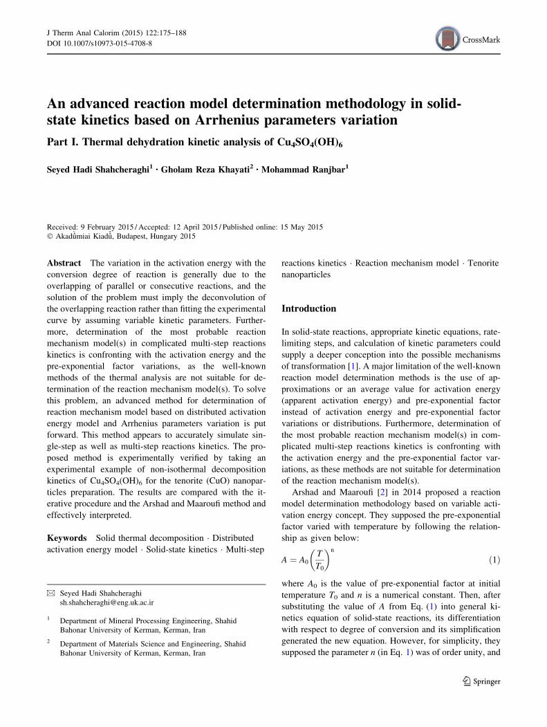
An advanced reaction model determination methodology in solid-state kinetics based on Arrhenius parameters variation

Part I. Thermal dehydration kinetic analysis of Cu4SO4(OH)6

Seyed Hadi Shahcheraghi1 • Gholam Reza Khayati2 • Mohammad Ranjbar1

Received: 9 February 2015 / Accepted: 12 April 2015 / Published online: 15 May 2015

� Akadumiai Kiadu, Budapest, Hungary 2015

Abstract The variation in the activation energy with the

conversion degree of reaction is generally due to the

overlapping of parallel or consecutive reactions, and the

solution of the problem must imply the deconvolution of

the overlapping reaction rather than fitting the experimental

curve by assuming variable kinetic parameters. Further-

more, determination of the most probable reaction

mechanism model(s) in complicated multi-step reactions

kinetics is confronting with the activation energy and the

pre-exponential factor variations, as the well-known

methods of the thermal analysis are not suitable for de-

termination of the reaction mechanism model(s). To solve

this problem, an advanced method for determination of

reaction mechanism model based on distributed activation

energy model and Arrhenius parameters variation is put

forward. This method appears to accurately simulate sin-

gle-step as well as multi-step reactions kinetics. The pro-

posed method is experimentally verified by taking an

experimental example of non-isothermal decomposition

kinetics of Cu4SO4(OH)6 for the tenorite (CuO) nanopar-

ticles preparation. The results are compared with the it-

erative procedure and the Arshad and Maaroufi method and

effectively interpreted.

Keywords Solid thermal decomposition � Distributed

activation energy model � Solid-state kinetics � Multi-step

reactions kinetics � Reaction mechanism model � Tenorite

nanoparticles

Introduction

In solid-state reactions, appropriate kinetic equations, rate-

limiting steps, and calculation of kinetic parameters could

supply a deeper conception into the possible mechanisms

of transformation [1]. A major limitation of the well-known

reaction model determination methods is the use of ap-

proximations or an average value for activation energy

(apparent activation energy) and pre-exponential factor

instead of activation energy and pre-exponential factor

variations or distributions. Furthermore, determination of

the most probable reaction mechanism model(s) in com-

plicated multi-step reactions kinetics is confronting with

the activation energy and the pre-exponential factor var-

iations, as these methods are not suitable for determination

of the reaction mechanism model(s).

Arshad and Maaroufi [2] in 2014 proposed a reaction

model determination methodology based on variable acti-

vation energy concept. They supposed the pre-exponential

factor varied with temperature by following the relation-

ship as given below:

A ¼ A0

T

T0

� �n

ð1Þ

where A0 is the value of pre-exponential factor at initial

temperature T0 and n is a numerical constant. Then, after

substituting the value of A from Eq. (1) into general ki-

netics equation of solid-state reactions, its differentiation

with respect to degree of conversion and its simplification

generated the new equation. However, for simplicity, they

supposed the parameter n (in Eq. 1) was of order unity, and

& Seyed Hadi Shahcheraghi

[email protected]

1 Department of Mineral Processing Engineering, Shahid

Bahonar University of Kerman, Kerman, Iran

2 Department of Materials Science and Engineering, Shahid

Bahonar University of Kerman, Kerman, Iran

123

J Therm Anal Calorim (2015) 122:175–188

DOI 10.1007/s10973-015-4708-8

http://crossmark.crossref.org/dialog/?doi=10.1007/s10973-015-4708-8&domain=pdf

http://crossmark.crossref.org/dialog/?doi=10.1007/s10973-015-4708-8&domain=pdf

the term [b (n ? Ea/RT)/T] was approximated to [bEa/RT2]

due to high values of activation energy of solid-state re-

actions, where b is the heating rate, R is the gas constant,

and Ea is the apparent activation energy. Generally, the

parameter n (in Eq. 1) is not of order unity, necessarily [3].

Also, the activation energies of solid-state reactions

essentially are not enough high to compensate this as-

sumption. For example, the activation energy variations for

the kinetics of non-isothermal and isothermal curing reac-

tion of DGEBA (diglycidyl ether of bisphenol-A) with a

nonlinear star-like aliphatic polyamine curing agent for epoxy

resins, N,N,N0,N0,N00-penta(3-aminopropyl)-diethylenetri-

amine (PADT), are between 20 and 56 kJ mol-1 [4]. Also,

the activation energy variations for the kinetics of DGEBA

thermosets cured with a hyperbranched poly (ethyleneimine)

and an aliphatic triamine are between 40 and 60 kJ mol-1 [5].

Hence, even though the methodology describes the ki-

netics of non-isothermal curing reaction of DGEBA with

an aliphatic diamine (to yield epoxy resin) well, it will not

probably be comprehensive method for determination of

mechanism model(s) of solid-state reactions.

To improve the conceptual principle of reaction kinetics,

an advanced method of reaction mechanism model deter-

mination based on Arrhenius parameters variation is put

forward. This method appears to accurately simulate sin-

gle-step as well as multi-step reactions kinetics. The pro-

posed method is verified by taking an experimental

example of non-isothermal decomposition kinetics of

Cu4SO4(OH)6. Then, the results are compared with it-

erative procedure and methodology of Arshad and Maar-

oufi [2] and effectively interpreted.

To the best of our knowledge, non-isothermal kinetics

modeling of CuO nanoparticles preparation from industrial

leaching solution has not been investigated yet. Our current

contribution will provide the comprehensive data toward a

better understanding of the mechanism(s) of Cu4SO4(OH)6

dissociation.

Koga et al. [6] in 1997 studied the reaction pathway of

the thermal decomposition of synthetic brochantite [Cu4

SO4(OH)6], which was prepared by the precipitates of basic

copper (II) sulfate at 298 K by adding 0.1 M NaOH solu-

tion dropwise at the rate of 1.0 mL min-1 with stirring to

100 mL of 0.1 M CuSO4 solution until the pH of the re-

sulting solution was equal to 8.0. The results showed that

the dehydration process was characterized by dividing into

two kinetic processes with a possible formation of an in-

termediate compound, Cu4O(OH)4SO4, which was fol-

lowed by the crystallization mixture of CuO and

CuO�CuSO4 at around 776 K. Moreover, the thermal

desulferation process was influenced by the gross diffusion

of the gaseous product SO3, which was governed by the

advancement of the overall reaction interface from the top

surface of the sample particle assemblage to the bottom.

In the present work, we studied only the thermal dehy-

dration kinetics of Cu4SO4(OH)6. Also, other stages of

thermal decomposition of Cu4SO4(OH)6 will be studied in

future works.

Materials and methods

Synthesis of precursor from pregnant leach solution

(PLS)

Copper leaching, solvent extraction and electrowinning are

the main hydrometallurgical processes for oxidized and

low-grade copper ore processing. Leaching involves dis-

solving Cu2? from copper-containing minerals into an

aqueous H2SO4 solution, known as the lixiviant, to produce

a pregnant leach solution (PLS). In addition to copper, the

PLS will also contain other impurity species, such as Fe,

Al, Co, Mn, Zn, Mg, and Ca, that may be present in the ore

and are leached with the copper [7–11]. In the present

work, the PLS was obtained from the industrial copper

heap-leaching solution of Miduk Copper mine in Iran.

In the present study, the solvent extraction process was

used for the purification of PLS. In copper solvent ex-

traction, the aqueous copper leach solution is concentrated

and purified using a copper-selective organic solution. The

solvent extraction process consists of extraction and strip-

ping processes, both of which may contain parallel and

series unit processes. In the extraction stage, the copper is

extracted from the leach solution into the organic solution

[7–11]. In the Miduk copper mine, 5-nonylsalicylaldoxime

is widely used as an organic extractant.

The concentration of solvent extractor in organic phase

(5-nonylsalicylaldoxime) was 8 %. The rest of the organic

phase was the proprietary diluent (a mixture of kerosene:

36 %, RESOL 8411: 30 %, and RESOL 8401: 26 %). One

liter of the organic phase was added to 1 L of leaching

solution in a separating funnel. The mixture was shaken

thoroughly for 4 min. After separation of the two phases,

the aqueous phase was put aside, and solvent extraction

was done on the organic phase again.

Then, an equal volume of sulfuric acid solution (200 g L-1)

was added to the separating funnel which contained the organic

phase. After mixing and separation of two phases, the organic

phase was put aside, and the aqueous phase which contained

CuSO4 was used for the synthesis of precursor.

The inductive coupled plasma (ICP-MS, Varian 715-ES)

analysis of the PLS and aqueous solution after stripping

(diluted CuSO4) was reported in Table 1. Accordingly, the

impurity species amounts of aqueous solution after strip-

ping are lower than 100 mg L-1, and there was no sig-

nificant effect on the run of Cu4SO4(OH)6 decomposition

[12–16].

176 S. H. Shahcheraghi et al.

123

Brochantite [Cu4SO4(OH)6], as precursor, was prepared

by the addition of a 0.5 M Na2CO3 solution to a 0.05 M

(2.56 g L-1) previous stage CuSO4 solution at a rate of

4 mL min-1 (dropwise) for 95 min with vigorous stirring

(1500 rpm) at 55 �C. The green precipitate (brochantite)

was then filtered and rinsed three times with warm deion-

ized water and dried at 50 �C for several hours.

Methods of sample characterization

To study the kinetics of Cu4SO4(OH)6 decomposition,

7 ± 0.5 mg of the precursor is studied through DSC–TG

(German NETZSCH-STA409C thermal analyzer) in a dy-

namic (50 mL min-1) atmosphere of argon at different

heating rates of 5, 10, 15, and 20 �C min-1 in the tem-

perature range of 25–800 �C. For each sample and heating

rate, three repetitive TG curves were obtained to assure

reproducibility of the results.

The crystalline structures, morphology, and size of CuO

nanoparticles were characterized by XRD (Philips, X’pert-

MPD system using Cu Ka) and SEM (Tescan Vega), respec-

tively. The morphology of the synthesized brochantite [Cu4-

SO4(OH)6] was examined by HRSEM (Hitachi S-4160). IR

spectra were recorded in the 400–4000 cm-1 range with a

resolution of 4 cm-1, using Bruker tensor 27 FTIR spec-

trometer with RT-DIATGS detector and KBr pellet technique.

Nitrogen adsorption/desorption isotherms were mea-

sured by ASAP 2020 Micromeritics surface area analyzer.

The specific surface areas were assessed according to the

standard Brunauer–Emmett–Teller (BET) method. The

pore size distributions and total pore volume were deter-

mined from adsorption branches of isotherms by the Bar-

rett–Joyner–Halenda (BJH) method.

Theoretical

Theoretical background of solid-state kinetics

Generally, the rate of degradation reaction can be described

in terms of two functions, i.e., k(T) and f(a), thus,

dadt

¼ bdadT

¼ k Tað Þf að Þ ð2Þ

where a is the degree of conversion, t is the reaction time,

Ta is the absolute temperature, b is the heating rate, k(Ta) is

the rate constant, and f(a) is the type of reaction or function

of reaction mechanism. In TG analysis, the degree of

conversion can be defined as the ratio of actual mass loss to

the total mass loss corresponding to the decomposition

process [17–20]:

a ¼ m0 � m

m0 � mf

ð3Þ

where m0, m, and mf are the initial, actual, and final masses

of the sample, respectively. The dependence of the reaction

rate constant on temperature can be described by Arrhenius

equation [17, 21–23]:

k Tð Þ ¼ Aa exp � Ea

RTa

� �ð4Þ

where Aa is the pre-exponential factor, R is the gas constant

(8.314 J mol-1 K-1), and Ea is the apparent activation

energy. To estimate activation energy, various methods

have been proposed. These methods can be generally

categorized as: (a) isoconversional and (b) model-fitting

methods [21–25]. In addition, there are more complex

‘‘model-free’’ methods, such as the nonlinear isoconver-

sional method by Vyazovkin and Wight [26] and Vya-

zovkin [27], solutions of which can only be obtained using

computer algorithms.

Due to great calculation accuracy and versatile appli-

cability for various heating programs [21–23, 28], the ad-

vanced isoconversional methods developed by Vyazovkin,

the Vyazovkin method, was adopted to analyze the non-

isothermal reaction. Specifically, the Vyazovkin method is

applicable to a non-isothermal kinetic process with a series

of linear heating, which can be written as [17, 21–23]:

UðEaÞ ¼Xni¼1

Xnj 6¼1

IðEa; Ta;iÞbj

IðEa Ta;jÞbi

ð5Þ

I Ea; Ta;i� �

¼ZTa

Ta�Da

exp � Ea

RTa

� �dT ð6Þ

where bi and bj represent the different heating rates, Ta and

Ta-Da are the reaction temperatures corresponding to a and

Da, respectively. Minimizing Eq. (5) for each a with a

certain conversion increment (usually Da = 0.05) results

in the correction of Ea with a. The detailed descriptions of

how to use the Vyazovkin method to treat calorimetric data

can be acquired elsewhere [17, 21–23, 29, 30].

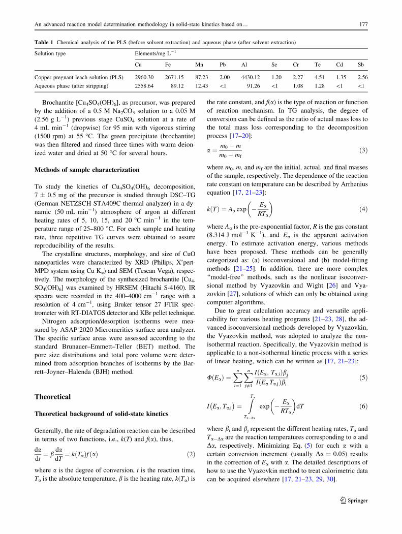
Table 1 Chemical analysis of the PLS (before solvent extraction) and aqueous phase (after solvent extraction)

Solution type Elements/mg L-1

Cu Fe Mn Pb Al Se Cr Te Cd Sb

Copper pregnant leach solution (PLS) 2960.30 2671.15 87.23 2.00 4430.12 1.20 2.27 4.51 1.35 2.56

Aqueous phase (after stripping) 2558.64 89.12 12.43 \1 91.26 \1 1.08 1.28 \1 \1

An advanced reaction model determination methodology in solid-state kinetics based on… 177

123

Arshad and Maaroufi method

Arshad and Maaroufi [2] in 2014 proposed a reaction

model determination methodology based on variable acti-

vation energy concept. They supposed the pre-exponential

factor varied with temperature by Eq. (1). Then, after

substituting the value of A from Eq. (1) into Eq. (2), its

differentiation with respect to degree of conversion and its

simplification (for simplicity, they supposed n = 1 (in

Eq. 1) and the term [b (n ? Ea/RT)/T] & [bEa/RT2] due to

high values of activation energy of solid-state reactions)

generated the following equation [2]:

h að Þ ¼ f 0 að Þf að Þ ¼ 1

dadt

! d2adt2

� �dadt

� � þ bRT

dEa

dT� bEa

RT2

24

35 ð7Þ

where h(a) is an expression to describe the ratio between

differentiated and actual reaction model.

The iterative procedure

The iterative procedure [31–35] is widely used to estimate

the most correct reaction mechanism, i.e., g(a) function,

ln g að Þð Þ ¼ lnAaEa

R

� �þ ln

exp �uað Þu2a

� �þ ln h uað Þð Þ

�

� ln bð Þð8Þ

where ua = Ea/RTa, and h(ua) is expressed by the fourth

Senum and Yang approximation formulas [21–23]. The de-

grees of conversion a corresponding to multiple rates at the

same temperature are in the left side of Eq. (8); combined

with well-known mechanism functions (Table 2), the slope of

the straight line and the linear correlation coefficient (r) is

obtained from the plot of ln(g(a)) versus ln(b). The most

probable mechanism function is the one for which the value

of the slope is near 1, and the correlation coefficient is higher.

If several g(a) functions follow this requirement, the

degrees of conversion corresponding to multiple heating

rates at several temperatures are used to calculate the most

probable mechanism by the same method. The function,

whose slope value is the closest to 1 and the correlation

coefficient that is also high at all these temperatures, is

considered to be the most probable mechanism function. In

this work, the proposed method results are compared with

iterative procedure and the Arshad and Maaroufi method.

Distributed activation energy model (DAEM)

The DAEM is a powerful method that has been used very

successfully in the kinetic analysis of complex materials

[36–38]. The model assumes that many irreversible first-order

parallel reactions that have different rate parameters and a

Gaussian distribution of activation energies occur simultane-

ously. The DAEM can be described by Eq. (9) [36–38]:

1 � a ¼Z1

0

exp �ZT

0

Aa

bexp � Ea

RTa

� �dT

0@

1Af Eað ÞdEa

ð9Þ

where f(Ea) is the distribution curve of the activation en-

ergy to represent the differences in the activation energies

of many first-order irreversible reactions. A new method

was presented by Miura [36] for estimating f(Ea) and Aa in

the DAEM. He does not assume a predefined activation

energy distribution and supposes a non-constant frequency

factor [28]. In supposed method, f(Ea) and Aa can be

estimated accurately. The equation is expressed as

follows [36]:

lnbT2a

� �¼ ln

AaR

Ea

� �þ 0:6075 � Ea

RTað10Þ

The proposed method for determination of reaction

mechanism

Non-isothermal kinetics

Generally, in the thermal analysis, degree of conversion,

energy of activation, and pre-exponential factor vary in the

following way:

a ¼ x1 T ; tð Þ E ¼ x2 að Þ ¼ Ea A ¼ x3 að Þ ¼ Aa

The overall change in the reaction rate as reaction ad-

vances can be described by differentiating Eq. (2) with

respect to the degree of conversion as:

d

dadadt

� �¼ da

dt

1

Aa

dAa

da� 1

RTa

dEa

daþ Ea

RT2a

dTa

daþ f 0 að Þ

f að Þ

�

ð11Þ

Using chain rule of differentiation, d/da(da/dt) = d/

dt(da/dt)(dt/da) = (d2a/dt2)/(da/dt), and rearranging

Eq. (11) give:

d2adt2

� �dadt

� �2¼ 1

Aa

dAa

da� 1

RTa

dEa

daþ Ea

RT2a

dTa

daþ f 0 að Þ

f að Þ

� ð12Þ

On the basis of Eq. (10), the pre-exponential factor can

be written as:

Aa ¼ EabRCT2

aexp

Ea

RTa

� �ð13Þ

where C is a numerical constant. Substituting the

value of Aa from Eq. (13) into Eq. (12) yields the fol-

lowing equation:


123

d2adt2

� �dadt

� �2¼ 1

Ea

dEa

da� 2

Ta

dTa

da

� �þ f 0 að Þ

f að Þ

� ð14Þ

Employing chain rule of differentiation, dEa/da = (dE/

dT)(dT/da) = b(dE/dT)/(da/dt) and also dTa/da = 1/(da/

dT) = b/(da/dt), and substituting them into Eq. (14) yield

the following equation:

Table 2 Mathematical expressions of functions g(a) and f(a) with their physical meanings

No. Model g(a) f(a) Rate-determining mechanism

1. Chemical process or

mechanism non-invoking

equations

F1/3 1 - (1 - a)2/3 (3/2)(1 - a)1/3 Chemical reaction

F3/4 1 - (1 - a)1/4 (4)(1 - a)3/4 Chemical reaction

F3/2 (1 - a)-1/2 - 1 (2)(1 - a)3/2 Chemical reaction

F2 (1 - a)-1 - 1 (1 - a)2 Chemical reaction

F3 (1 - a)-2 - 1 (1/2)(1 - a)3 Chemical reaction

2. Acceleratory rate equations P3/2 a3/2 (2/3)a-1/2 Nucleation

P1/2 a1/2 2a1/2 Nucleation



E1 ln(a) a Nucleation

3. Sigmoidal rate equations or

random nucleation and

subsequent growth

A1, F1 -ln(1 - a) (1 - a) Assumed random nucleation and

its subsequent growth, n = 1

A3/2 [-ln(1 - a)]2/3 (3/2)(1 - a)[-ln(1 - a)]1/3 Assumed random nucleation and

its subsequent growth, n = 1.5

A2 [-ln(1 - a)]1/2 (2)(1 - a)[-ln(1 - a)]1/2 Assumed random nucleation and






Au ln[a/(1 - a)] a (1 - a) Branching nuclei

4. Deceleratory rate equations

(phase boundary reaction)

R1, F0,

P1

a 1 Contracting disk

R2, F1/

2

1 - (1 - a)1/2 (2)(1 - a)1/2 Contracting cylinder

R3, F2/

3

1 - (1 - a)1/3 (3)(1 - a)2/3 Contracting sphere


(based on the diffusion

mechanism)

D1 a2 1/(2a) One-dimensional diffusion

D2 a ? [(1 - a)ln(1 - a)] [-ln(1 - a)]-1 Two-dimensional diffusion

D3 [1 - (1 - a)1/3]2 (3/2)(1 - a)2/3[1 - (1 - a)1/3]-1 Three-dimensional diffusion,

spherical symmetry

D4 1 - (2a/3) - (1 - a)2/3 (3/2)[(1 - a)-1/3 - 1]-1 Three-dimensional diffusion,

cylindrical symmetry

D5 [(1 - a)-1/3 - 1]2 (3/2)(1 - a)4/3[(1 - a)-1/3 - 1]-1 Three-dimensional diffusion

D6 [(1 ? a)1/3 - 1]2 (3/2)(1 ? a)2/3[(1 ? a)1/3 - 1]-1 Three-dimensional diffusion

D7 1 ? (2a/3) - (1 ? a)2/3 (3/2)[(1 ? a)-1/3 - 1]-1 Three-dimensional diffusion

D8 [(1 ? a)-1/3 - 1]2 (3/2)(1 ? a)4/3[(1 ? a)-1/3 - 1]-1 Three-dimensional diffusion

6. Other kinetics equations

with unjustified mechanism

G1 1 - (1 - a)2 1/[(2)(1 - a)]

G2 1 - (1 - a)3 1/[(3)(1 - a)2]

G3 1 - (1 - a)4 1/[(4)(1 - a)3]

G4 [-ln(1 - a)]2 (1/2)(1 - a)[-ln(1 - a)]-1

G5 [-ln(1 - a)]3 (1/3)(1 - a)[-ln(1 - a)]-2

G6 [-ln(1 - a)]4 (1/4)(1 - a)[-ln(1 - a)]-3

G7 [1 - (1 - a)1/2]1/2 (4)[(1 - a)[1 - (1 - a)]1/2]1/2

G8 [1 - (1 - a)1/3]1/2 (6)(1 - a)2/3[1 - (1 - a)1/3]1/2


123

d2adt2

� �dadt

� �2¼ b

Ea

dEa

dT

1dadt

!� 2b

Ta

1dadt

!þ f 0 að Þ

f að Þ

" #ð15Þ

Rearrangement of Eq. (15) gives:

f 0 að Þf að Þ ¼ Sh að Þ ¼ 1

dadt

! d2adt2

� �dadt

� � � bEa

dEa

dTþ 2b

Ta

24

35 ð16Þ

where Sh(a) is the ratio between differentiated and actual

reaction model. It is clear from this equation that its right-

hand side can be obtained by experimental thermo-

analytical data, while left-hand side can be simulated for

the reaction models. A fair fitting between curves generated

from thermoanalytical data and theoretical models can re-

sult in the appropriate reaction models. Equation (16) takes

the following form when the reaction follows single-step

kinetics and dEa/dT & 0:

f 0 að Þf að Þ ¼ Sh að Þ ¼ 1

dadt

! d2adt2

� �dadt

� � þ 2bTa

24

35 ð17Þ

Moreover, if the difference between the maximum and

minimum values of Ea was less than 20–30 % of the av-

erage Ea, the activation energy was independent from a[28, 39]. In this state, because of dEa/dT = 0, Eq. (16) was

used for determination of reaction mechanism model.

Furthermore, the reaction model(s) for multi-step pro-

cesses could be determined using integration of Sh(a):

Z1

0

Sh að Þda ¼Z1

0

f 0 að Þf að Þ da ¼ f að Þ ð18Þ

Isothermal kinetics

Sh(a) in isothermal kinetics can be determined by putting

b = (dT/dt) = 0 in Eq. (16) and rearranging it as

following:

f 0 að Þf að Þ ¼ Sh að Þ ¼

d2adt2

� �dadt

� �2� 1

Ea

dEa

dað19Þ

In isothermal kinetics, the evaluation of reaction model

follows the similar route as discussed in the previous sec-

tion. If the reaction consists of only one step (dE/da & 0),

Eq. (19) can be written as following equation:

f 0 að Þf að Þ ¼ Sh að Þ ¼

d2adt2

� �dadt

� �2ð20Þ

It should be mentioned, if reaction follows single-step

isothermal kinetics then its mechanistic information can be

directly obtained by thermoanalytical data, independent of

its activation energy and pre-exponential factor. Table 3

represents the Sh(a) expression for well-known reaction

models.

Results and discussion

Preparation of CuO nanoparticles

Figure 1a shows the XRD pattern of Cu4SO4(OH)6 pre-

cursor. As shown, almost all diffraction peaks were con-

sistent with monoclinic Cu4SO4(OH)6 (JCPDS card No.

01-087-0454). Figure 1b shows typical XRD pattern of

CuO nanocrystals prepared at the heating rate of

10 �C min-1. As shown, all the diffraction peaks of

nanoparticles (i.e., 32.51, 35.56, 38.74, 46.31, 48.75, 53.51,

58.31, 61.53, 66.24, and 68.13) are consistent with the

standard structure (JCPDS card no. 05-0661). Accordingly,

the precursor was completely decomposed at about 700 �Cinto single phase of the pure crystalline CuO. It is well

known that crystallite size can be estimated from diffrac-

tion pattern analysis by measuring the full width at half

maximum (FWHM) measurement and applying the

Scherrer equation [40]:

D ¼ lkbCos h0ð Þ ð21Þ

where b is the FWHM, l is the Scherrer constant (l = 0.9)

[12–16, 40, 41], k is the wavelength in nanometers (the

wavelength of Cu Ka is 0.154 nm [12, 13, 41]), h0 is the

Bragg angle, and D the mean crystallite size (nm) [40]. The

peak broadening also depends on the lattice strain induced

by mechanical stresses, so that the Williamson–Hall

method can be used to improve the analysis [42]. The mean

crystallite size of tenorite was calculated to be about 45 nm

using Scherrer equation.

Figure 2a, b shows the FT-IR spectra of the Cu4SO4(-

OH)6 precursor and the CuO nanoparticles prepared at the

heating rate of 10 �C min-1. The absorption bands

(Fig. 2a) around 426, 487, 511, 601, 735, 780, 875, 943,

988, 1088, 1126, 1431, 3275, and 3391 cm-1 are attributed

to Cu4SO4(OH)6 [43, 44]. In Fig. 2b, the peak around

480–585 cm-1 is assigned to Cu–O of CuO, confirming the

formation of the pure CuO nanoparticles [45–47]. And,

the peak at 2363 cm-1 corresponds to the atmospheric

CO2 [48].

Figure 3a shows the typical SEM image of CuO

nanoparticles prepared at the heating rate of 10 �C min-1.

Accordingly, CuO particles exhibit a strong tendency to

form nanoparticle agglomerates. Moreover, in the Scherrer

method, the average crystallite size of CuO (i.e., 45 nm)

was calculated and is not necessarily equal to the particle


123

size of CuO (Fig. 3a). According to the literature, these

differences can be related to the agglomeration and sin-

tering of particles during the heating process [49–52]. The

solid-state reconstruction of nanoparticles into aggregates

is a usual phenomenon showing a tendency of nanopar-

ticulate systems to restrain unsaturated surface forces via

surface recombination [53–55]. EDX analysis of CuO

nanoparticles (Fig. 3b) confirms the high purity of the

products.

Non-isothermal decomposition of the CuO

nanoparticle precursor

The DSC–TG curves of non-isothermal degradation of the

CuO nanoparticle precursor at four different heating rates

(5, 10, 15, and 20 �C min-1) are shown in Fig. 4. Ac-

cordingly, mass losses within three broad steps (about 7, 9,

and 12 mass%) were found between 61 and 717 �C. Fur-

thermore, the overall mass loss during decomposition of

Table 3 Mathematical expressions of functions Sh(a) for the well-known reaction functions

No. Model f(a) Sh(a)

1. Chemical process or mechanism

non-invoking equations

Fn (n = 0,1/2,2/3,1) (1 - a)n/|1 - n| -n/(1 - a)

2. Acceleratory rate equations Pn (n = 1) (1/n)a(1-n) (1 - n)/a

E1 a 1/a

3. Sigmoidal rate equations or random

nucleation and subsequent growth

An n(1 - a)[-ln(1 - a)](1-1/n) [1 - (1/n) ? ln(1 - a)]/[(a - 1)

ln(1 - a)]

F1 (1 - a) 1/(a - 1)


(phase boundary reaction)

R1, F0, P1 1 0

Rn (n = 2,3) (n)(1 - a)1-1/n (1 - n)/[n(1 - a)]

Fn (n = 1/2,2/3) (1 - a)n/|1 - n| -n/(1 - a)


(based on the diffusion mechanism)

D1 1/(2a) -1/a

D2 [-ln(1 - a)]-1 [1/(1 - a)]/ln(1 - a)

D3 (3/2)(1 - a)2/3[1 - (1 - a)1/3]-1 -(2/3)(1 - a)-1[1 ? [(1/2)(1 - a)1/3

(1 - (1 - a)1/3)-1]]

D4 (3/2)[(1 - a)-1/3 - 1]-1 (1/3)(1 - a)-4/3[(1 - a)-1/3 - 1]-1

D5 (3/2)(1 - a)4/3[(1 - a)-1/3

- 1]-1-(4/3)(1 - a)-1[1 ? [(1/4)(1 - a)-1/3

((1 - a)-1/3 - 1)-1]]

D6 (3/2)(1 ? a)2/3[(1 ? a)1/3-1]-1 (2/3)(1 ? a)-1[1 - [(1/2)(1 ? a)1/3

(1 - (1 ? a)1/3)-1]]

D7 (3/2)[(1 ? a)-1/3-1]-1 -(1/3)(1 ? a)-4/3[(1 ? a)-1/3 - 1]-1

D8 (3/2)(1 ? a)4/3[(1 ? a)-1/3-1]-1 (4/3)(1 ? a)-1[1 ? [(1/4)(1 ? a)-1/3

((1 ? a)-1/3-1)-1]]

6. Sestak–Berggren (autocatalytic model) SB(m,n) am(1 - a)n (m/a) - (n/(1 - a))

3000

2500

2000

1500

1000

500

020 30 40 50 60 70

Inte

nsity

/a.u

.

Cu4SO4 (OH)6

CuO

(220

)

(221

)_

(222)_ (2

32)_

(322

)_(402

)_

(400

)

(230

)

(420

)(3

30)

(140

)

(240

)(5

20)

(232

)_

(512

) _(4

42)

_(3

52) _

(204

) _(1

62)

_ (311

)

_ (113

)

_ (202

)

_ (112

)

_ (111

)

_(4

32) _

(313

)

(610

)(530)

(620

)

(151

)

(550

)(2

52)

(220

)

(202

)

(020

)

(111

)

(110

)

(b)

(a)

(a)

(b)

2θ/°

Fig. 1 a XRD pattern of the precursor Cu4SO4(OH)6 and b XRD

pattern of CuO nanoparticles prepared at the heating rate of

10 �C min-1

3500 3000 2500 2000 1500 1000 500

Wavenumber/cm–1

Tra

nsm

ittan

ce/%

3586

.51

3564

.19

3531

.69

3391

.15

2363

.73

2362

.72

1651

.00

1631

.47

1515

.32

1431

.10

1389

.68

1385

.93

1125

.92

1088

.66

988.

4594

3.08

875.

3482

2.11

780.

5073

5.15

601.

1954

1.10

511.

6048

7.27

485.

3942

6.47

(a)

(b)1520

2530

3540

Fig. 2 a FT-infrared spectrum of the precursor Cu4SO4(OH)6 and

b FT-infrared spectra of the CuO nanoparticles


123

Cu4SO4(OH)6 to CuO as well as stages I and II of dehy-

dration was calculated on the basis of stoichiometric che-

mical equations, and similar mass reduction was observed.

The first and second one which are between 61 and 250 �Care related to the thermal dehydration that proceeded

through the following two processes, respectively [6]:

Cu4SO4 OHð Þ6 ! Cu4SO4O OHð Þ4þH2O ð22Þ

Cu4SO4O OHð Þ4 ! Cu4SO4O3 þ 2H2O ð23Þ

The third one which is between 622 and 717 �C is re-

lated to the desulferation process. DSC of the precursor

(Fig. 4) shows three endothermic peaks around 102 �C(dehydration I), 223 �C (dehydration II), and 700 �C(desulferation) and one exothermic peak, at 541 �C. The

exothermic peak between 500 and 600 �C may be due to

the crystallization of the amorphous dehydrated product

(Cu4SO4O3) to CuO and CuO�CuSO4 [6].

The same results were obtained in TG analysis, which

shows no loss in mass between 533 and 556 �C. Hence, it

can be concluded that the endothermic peak at 700 �C is

due to the decomposition of the copper oxide sulfate

[CuO�CuSO4] to CuO [6, 56]. Moreover, by increasing the

heating rate, the TG curve and peak of DSC curve shift to a

higher temperature, and the final mass loss presents a de-

creasing trend.

From Fig. 4, by increasing the heating rate, the reaction

area was shifted to a higher temperature range. Moreover,

onset reaction temperatures, peak temperatures, and end

temperatures enhanced with increasing heating rate

(Table 4). In the present study, the thermal dehydration

kinetics of Cu4SO4(OH)6 was studied. Furthermore, other

stages of thermal decomposition of Cu4SO4(OH)6 will be

studied in future work.

The conversional curves (a–T) for thermal dehydrations

(I and II) of Cu4SO4(OH)6 are indicated in Fig. 5. These

conversional curves exhibit the sigmoidal profile, and by

increasing heating rate, the curves shift toward the higher

temperature. In other words, the higher the heating rate, the

higher the temperature for the reaction to reach the iden-

tical a.

Calculation of activation energy (Ea)

The dependence of Ea on a for thermal dehydrations (I and

II) of Cu4SO4(OH)6 is presented in Fig. 6. According to the

literature [57–61], if Ea values were independent of a, the

decomposition process was dominated by a single reaction

step. Therefore, from Fig. 6, it was obvious that thermal

dehydration I and dehydration II are a single-step process,

but dE/dT = 0. Based on the Vyazovkin method, Ea

showed an almost stable behavior with the average of

Ea = 32.3 ± 2.1 and 63.9 ± 1.1 kJ mol-1 for thermal

dehydration I and dehydration II, respectively, which are

more lower than values of the literature (Koga et al. [6],

Fig. 3 a Typical SEM image of

CuO nanoparticles prepared at

the heating rate of 10 �C min-1

at 320,000 magnification,

b EDS patterns of CuO

nanoparticles

100

90

80

70

600 200 400 600 800

1

–1

–3

–5

–70 200 400 600 800

Temperature/°C

Temperature/°C

Mas

s/%

Hea

t flo

w/W

g–1

EX

O

5 °C min–1

10 °C min–1

15 °C min–1

20 °C min–1

(a)

(b)

5 °C min–1

10 °C min–1

15 °C min–1

20 °C min–1

Fig. 4 a TG and b DSC curves for thermal decomposition of

precursor Cu4SO4(OH)6 at the heating rates of 5, 10, 15, and

20 �C min-1 in argon


123

i.e., 158.0 ± 1.3 and 193.1 ± 0.9 kJ mol-1 for thermal

dehydration I and dehydration II, respectively). It could be

related to the nanostructure of the synthetic brochantite

[Cu4SO4(OH)6] in the present study.

The suitable kinetics models for describing thermal

dehydrations (I and II) of Cu4SO4(OH)6 were determined

using the proposed method, and obtained results were

compared with the iterative procedure.

Determination of the most probable reaction

mechanism function

The proposed method

To verify the validity of the proposed method, thermal

decomposition kinetics of Cu4SO4(OH)6 were considered,

and obtained results were compared with the iterative

procedure and the Arshad and Maaroufi method. From

Fig. 6, for thermal dehydrations (I and II) of Cu4SO4(OH)6,

dE/dT = 0. Hence, the evaluation of the most probable

reaction mechanism function using the proposed method

follows Eq. (16).

The Sh(a) curves for the thermoanalytical data of the

thermal dehydrations (I and II) of Cu4SO4(OH)6 at

b = 10 �C min-1 are presented in Fig. 7a, b, respectively.

As shown, the Sh(a) curves form follows the Avrami–

Erofeev Am-type equation, m(1 - a)[-ln(1 - a)](1-1/m),

i.e., m = 1.453 (which belongs to diffusion controlled

[62]) and m = 1.908 (which belongs to interface controlled

[62]), for thermal dehydrations I and II, respectively. The

reaction model parameters (proposed method) are given in

Table 5. Accordingly, as shown in Fig. 7a, b, there was a

good agreement between the experimentally obtained

Table 4 Typical parameters of the thermal dehydration of precursor

Cu4SO4(OH)6

Reaction Heating rate/

�C min-1Tonset/�C Tpeak/�C Tend/�C

Dehydration I 5 49 97 133

10 61 102 142

15 75 119 166

20 94 130 174

Dehydration II 5 197 214 241

10 201 223 249

15 212 237 274

20 228 251 286

30

20

10

0

–10

–20

–300.0 0.1 0.2 0.3 0.5 0.6 0.7 0.8 0.9 1.00.4

0.0 0.1 0.2 0.3 0.5 0.6 0.7 0.8 0.9 1.00.4

30

20

10

0

–10

–20

–30

α

α

f' (α

)/f(

)

Simulated by proposed methodSimulated by Arshad and Maaroufi methodExperimental

Simulated by proposed methodSimulated by Arshad and Maaroufi methodExperimental

(a)

(b)

αf' (

α)/f

()

α

Fig. 7 Agreement between the experimentally obtained Sh(a) curve

and proposed method obtained Sh(a) curve and comparison of results

with Arshad and Maaroufi method (b = 10 �C min-1) for a the

thermal dehydration I and b dehydration II of precursor Cu4SO4

(OH)6; Sh(a) values follow Eq. (16)

1.0

0.8

0.6

0.4

0.2

0.050 100 150 200 250 300 350

Temperature/°C

α

Dehydration I

Dehydration II

5 °C min–1

10 °C min–1

15 °C min–1

20 °C min–1

Fig. 5 a–T curves for the thermal dehydrations I and II of precursor

Cu4SO4(OH)6 at the heating rates of 5, 10, 15, and 20 �C min-1 in

argon, where a is the degree of conversion and can be well calculated

by Eq. (3)

75

60

45

30

15

00.0 0.2 0.4 0.6 0.8 1.0

Conversion

Act

ivat

ion

ener

gy/k

J m

ol–1

Dehydration I

Dehydration II

Fig. 6 Dependence of activation energy (Ea) on conversion (a) for

the thermal dehydrations I and II of precursor Cu4SO4(OH)6


123

Sh(a) curves and Am model obtained Sh(a) curves

(b = 10 �C min-1).

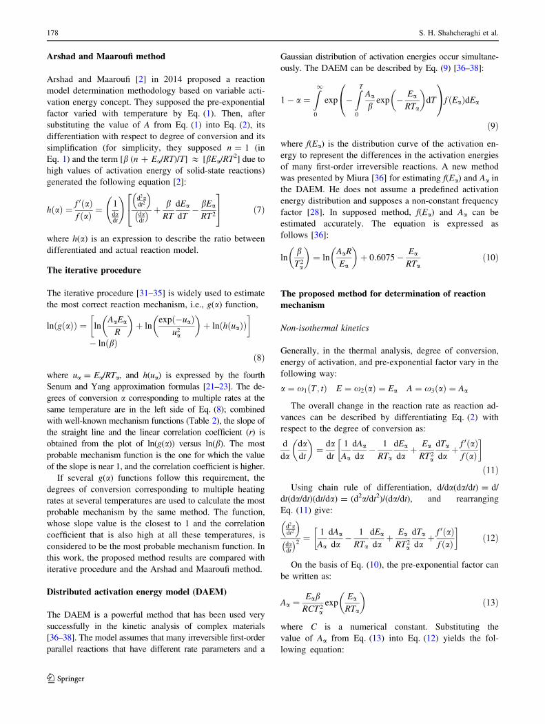
Moreover, these results were proved by the HRSEM

(Fig. 8) and BET (Fig. 9). As shown in Fig. 8, the

brochantite [Cu4SO4(OH)6] nanoparticles have strong ten-

dency to agglomeration. Therefore, according to Eq. (22),

for the thermal dehydration I, some of the OH molecules are

aspirated from agglomerated precursor with the mechanism

of diffusion controlled, and the porous precursor is made.

Then, according to Eq. (23), for the thermal dehydration II,

the residual OH molecules are aspirated from porous pre-

cursor with the mechanism of interface controlled, and the

amorphous precursor is made in view of XRD.

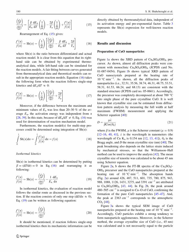
Also, the strong agglomerated structure of precursor and

the porous sample structure of the thermal dehydration I

were investigated by BET analysis. The data in Fig. 9

display the N2 adsorption–desorption isotherms confirmed

the strong agglomeration of precursor and the porous

sample of the thermal dehydration I.

According to the classification given by Brunauer et al.

[63, 64], the isotherms determined on both samples are

similar to type IV isotherms which are obtained for porous

materials (1.5 nm\ rp\ 100 nm). According to the

IUPAC classification [65], the isotherm determined on the

as-received precursor exhibits the type H1 hysteresis loop

(Fig. 9a). The type H1 hysteresis loop is attributed to the

formation of spherical shape pores with a narrow pores

distribution [65, 66]. The BET analysis showed that the as-

received precursor structure is the characteristic of bi-

modal-typed pore size distribution in the range of 2–25 nm

(below 100 nm), which is due to the strong agglomeration

of the precursor nanoparticles (the inset in Fig. 9a).

Also, the isotherm determined on the porous sample of

the thermal dehydration I exhibits the type H2 hysteresis

loop (Fig. 9b). The distribution of pore sizes and the pore

shape in H2 type is not well defined or irregular [65, 66].

Moreover, the type H2 loop is believed to be associated

with ink bottle-like pores of varying radius [67]. The BET

analysis showed that the porous sample structure of the

thermal dehydration I is the characteristic of pore size

distribution in the range of 2 nm to 100 nm, which could

be due to the strong porous structure of the thermal de-

hydration I sample (the inset in Fig. 9b).

The Arshad and Maaroufi method

To find the most probable reaction mechanism using the

Arshad and Maaroufi method, Eq. (7) is used. The h(a)

curves for the thermoanalytical data of the thermal

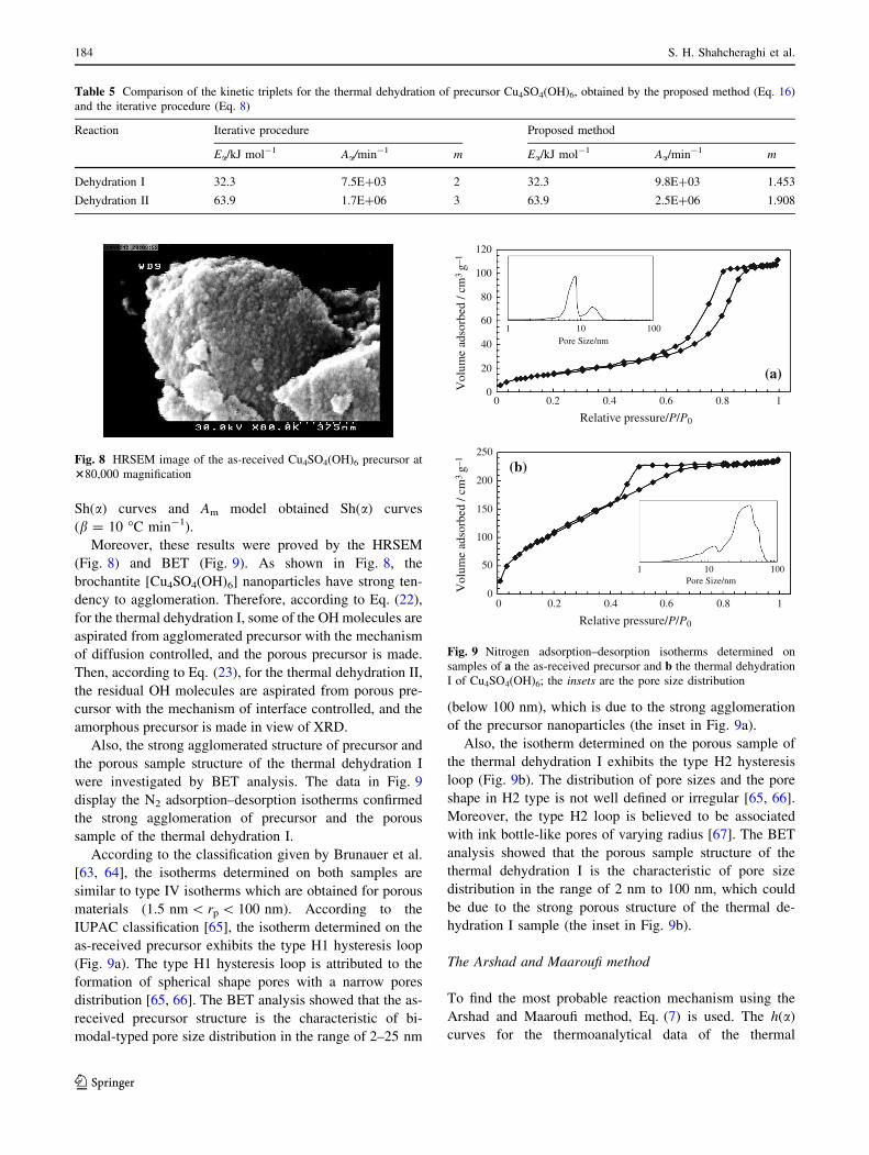
Table 5 Comparison of the kinetic triplets for the thermal dehydration of precursor Cu4SO4(OH)6, obtained by the proposed method (Eq. 16)

and the iterative procedure (Eq. 8)

Reaction Iterative procedure Proposed method

Ea/kJ mol-1 Aa/min-1 m Ea/kJ mol-1 Aa/min-1 m

Dehydration I 32.3 7.5E?03 2 32.3 9.8E?03 1.453

Dehydration II 63.9 1.7E?06 3 63.9 2.5E?06 1.908

Fig. 8 HRSEM image of the as-received Cu4SO4(OH)6 precursor at

380,000 magnification

120

100

80

60

40

20

00 0.2 0.4 0.6 0.8 1

Relative pressure/P/P0

Relative pressure/P/P0

250

200

150

100

50

00 0.2 0.4 0.6 0.8 1

Vol

ume

adso

rbed

/ cm

3 g–

1V

olum

e ad

sorb

ed /

cm3

g–1

1 10 100Pore Size/nm

1 10 100Pore Size/nm

(a)

(b)

Fig. 9 Nitrogen adsorption–desorption isotherms determined on

samples of a the as-received precursor and b the thermal dehydration

I of Cu4SO4(OH)6; the insets are the pore size distribution


123

dehydrations (I and II) of Cu4SO4(OH)6 at

b = 10 �C min-1 are presented in Fig. 7a, b, respectively.

As shown, the h(a) curves form for the thermal dehydra-

tions I and II follows the Am- and the Dn-type equations

[Deceleratory rate equations (based on the diffusion

mechanism)], respectively. Hence, the results of the Arshad

and Maaroufi method are not valid for the thermal dehy-

drations (I and II) of Cu4SO4(OH)6.

The iterative procedure

To find the most probable reaction mechanism using the

iterative procedure, Eq. (8) is used. The degrees of con-

version for b = 5, 10, 15, and 20 �C min-1 at the same

temperature for the thermal dehydrations (I and II) of

Cu4SO4(OH)6 are listed in Table 5. The appropriate tem-

peratures are randomly selected, and the range of a cor-

responding to the temperature should be within 0.1–0.9.

The corresponding degrees of conversion of three tem-

peratures are chosen as examples to put into 35 types of

mechanism functions (Table 1).

The slope, correlation coefficient, i.e., r, and intercept of

linear regression of ln(g(a)) versus ln(b) are obtained. The

results of the linear regression for the thermal dehydration I

of Cu4SO4(OH)6 show that the slopes of A2 (g(a) =

[-ln(1 - a)]1/2) mechanism function are the most adjacent

to 1, and the correlation coefficients are better, which are

listed in Table 6. Therefore, A2, which belongs to the

mechanism of interface controlled [62]), is determined to

be the most probable mechanism function of the thermal

dehydration I of Cu4SO4(OH)6.

Also, the results of the linear regression for the thermal

dehydration II of Cu4SO4(OH)6 show that the slopes of A3

(g(a) = [-ln(1 - a)]1/3) mechanism function are the most

adjacent to 1, and the correlation coefficients are better,

which are listed in Table 6. Therefore, A3, which belongs

to the mechanism of interface controlled [62]), is deter-

mined to be the most probable mechanism function of the

thermal dehydration II of Cu4SO4(OH)6. Therefore, ac-

cording to the iterative procedure, mechanism of the ther-

mal dehydrations I and II of Cu4SO4(OH)6 is the interface

controlled. Hence, even though the obtained model types

Table 6 Relation between temperature and degrees of conversion (a) at different heating rates b (�C min-1) and results of ln[g(a)] versus ln(b)

curves of four types of probable mechanism functions for the thermal dehydration of precursor Cu4SO4(OH)6

Reaction T/�C a Reaction function Slope r

b = 5/�C min-1 b = 10/�C min-1 b = 15/�C min-1 b = 20/�C min-1

Dehydration I 110 0.830 0.638 0.281 0.079 F2 -2.816 0.959

F3 -3.708 0.978

A2 -1.046 0.929

A3 -0.697 0.929

112 0.859 0.678 0.316 0.101 F2 -2.808 0.965

F3 -3.813 0.982

A2 -1.001 0.933

A3 -0.667 0.933

114 0.886 0.717 0.353 0.124 F2 -2.825 0.969

F3 -3.958 0.985

A2 -0.963 0.937

A3 -0.642 0.937

Dehydration II 236 0.995 0.880 0.352 0.031 F2 -6.094 0.987

F3 -9.512 0.999

A2 -1.707 0.913

A3 -1.138 0.913

237 0.996 0.901 0.389 0.039 F2 -6.168 0.989

F3 -9.835 0.999

A2 -1.643 0.916

A3 -1.096 0.917

238 0.998 0.919 0.427 0.051 F2 -6.380 0.993

F3 -10.423 1.000

A2 -1.594 0.920

A3 -1.063 0.919


123

by the proposed method and the iterative procedure are the

Avrami–Erofeev, the obtained mechanism results by the

iterative procedure are not proved using HRSEM and BET.

The reaction model parameters for the iterative procedure

are given in Table 5.

Calculation of pre-exponential factor (Aa)

If the reaction follows single-step kinetics and its reaction

model is known, Eq. (2) can be rearranged as follows:

lndadt

expEa

RT

� �� ¼ ln Aað Þ þ ln f að Þð Þ ð24Þ

Equation (24) is the equation of straight line with Ea as

the activation energy for the single-step reaction. The value

of pre-exponential factor can be calculated by the intercept

of the straight line. On the other hand, if the reaction fol-

lows multi-step kinetics, pre-exponential factor(s) at each

value of ‘‘a’’ can be calculated by Eq. (25) as:

lndadt

� �¼ � Ea

RTaþ ln Aaf að Þð Þ ¼ � Ea

RTaþ Ca ð25Þ

where Ca is the intercept of the straight line of ln(da/dt)

versus 1/Ta. If reaction model(s) in the multi-step kinetics

is/are known over the whole domain of a, then the fol-

lowing equation is helpful to determine the pre-exponential

factor(s) over that domain:

Ca ¼ ln Aaf að Þð Þ ! Aa ¼exp Cað Þf að Þ ð26Þ

The pre-exponential factors for the proposed method and

the iterative procedure are given in Table 5. Accordingly, the

comparison of theoretically fitted reaction rates of the ther-

mal dehydrations (I and II) of Cu4SO4(OH)6 under the two

methodologies in Fig. 10 (b = 10 �C min-1) emphasizes

that the proposed methodology seems more efficient than the

iterative procedure (and other well-known methods). It can

be mentioned that the proposed method provides basis for the

detection of a number of new reaction models capable of

dealing with complex processes which could be more com-

plicated mathematically.

Furthermore, it should be mentioned that the kinetics

results of the proposed method and iterative procedure

presented in the paper were obtained using the programs

compiled by ourselves with MATLAB.

Conclusions

The results showed that it is a major limitation that the

well-known reaction model determination methods are

according to either the choice of constant Arrhenius pa-

rameters (apparent activation energy, apparent pre-expo-

nential factor), the use of approximations or the focus on

the kinetic compensation principle. To solve this problem,

an advanced method for the determination of reaction

mechanism model based on the Arrhenius parameter var-

iations was proposed.

This method appears to accurately simulate single-step

as well as multi-step reactions kinetics. The proposed

method was experimentally verified by taking an ex-

perimental example of non-isothermal decomposition ki-

netics of Cu4SO4(OH)6 for the tenorite (CuO) nanoparticles

preparation. The results showed that

1. Based on the Vyazovkin method, Ea showed an almost

stable behavior with the average of Ea = 32.3 ± 2.1

and 63.9 ± 1.1 kJ mol-1 for thermal dehydration I

and dehydration II, respectively.

2. Based on the proposed method, the mechanism func-

tion form follows the Avrami–Erofeev Am-type equa-

tion, m(1 - a)[-ln(1 - a)](1 - 1/m), i.e., m = 1.453

(which belongs to diffusion controlled) and m = 1.908

(which belongs to interface controlled) for thermal

dehydrations I and II, respectively. Moreover, these

results were confirmed by the HRSEM (Fig. 8) and

BET (Fig. 9).

3. According to the Arshad and Maaroufi method, the

h(a) curves form for the thermal dehydrations I and II

followed the Am- and the Dn-type equation [Decel-

eratory rate equations (based on the diffusion mechan-

ism)], respectively. Hence, the results of the Arshad

and Maaroufi method are not valid for the thermal

dehydrations (I and II) of Cu4SO4(OH)6.

4. The comparison of theoretically fitted reaction rates of

the thermal dehydrations (I and II) of Cu4SO4(OH)6

under the two methodologies, i.e., the iterative proce-

dure and the proposed method, showed the proposed

methodology seems more efficient than the iterative

procedure.

0.40

0.30

0.20

0.10

0.00330 360 390 420 450 480 510

Temperature/K

β dα

/dT

/min

–1Dehydration II

Dehydration I

ExperimentalSimulated by Iterative procedureSimulated by proposed method

Fig. 10 Comparison of experimental reaction rate and that predicated

from the proposed method (Eq. 16) and the iterative procedure

(Eq. 8) versus temperature for the thermal dehydrations I and II of

precursor Cu4SO4(OH)6 at the heating rate of 10 �C min-1 in argon


123

5. The proposed methodology seems to be more efficient

than the Arshad and Maaroufi method and the iterative

procedure as well as other well-known methods.

Moreover, the proposed method provides basis for

the detection of a number of new reaction models

capable of dealing with complex processes which

could be more complicated mathematically.

References

1. Tomashevitch KV, Kalinin SV, Vertegel AA, Oleinikov NN, Ketsko

VA, Tretyakov YD. Application of non-linear heating regime for the

determination of activation energy and kinetic parameters of solid-

state reactions. Thermochim Acta. 1998;323:101–7.

2. Arshad MA, Maaroufi AK. An innovative reaction model deter-

mination methodology in solid state kinetics based on variable

activation energy. Thermochim Acta. 2014;585:25–35.

3. Carr RW. Modeling of chemical reactions. 1st ed. Amsterdam:

Elsevier Science; 2007.

4. Wan J, Bu ZY, Xu CJ, Li BG, Fan H. Preparation, curing kinetics,

and properties of a novel low-volatile starlike aliphatic-polyamine

curing agent for epoxy resins. Chem Eng J. 2011;171:357–67.

5. Santiago D, Francos XF, Ramis X, Salla JM, Sangermano M.

Comparative curing kinetics and thermal–mechanical properties

of DGEBA thermosets cured with a hyperbranched poly

(ethyleneimine) and an aliphatic triamine. Thermochim Acta.

2011;526:9–21.

6. Koga N, Criado JM, Tanaka H. Reaction pathway and kinetics of

the thermal decomposition of synthetic brochantite. J Therm

Anal. 1997;49:1467–75.

7. Schlesinger ME, King MJ, Sole KC, Davenport WG. Extractive

metallurgy of copper. 5th ed. Amsterdam: Elsevier; 2011.

8. Kislik VS. Solvent extraction: classical and novel approaches. 1st

ed. Amsterdam: Elsevier; 2012.

9. Greenawalt WE. Hydrometallurgy of copper. 1st ed. West

Stockbridge, MA: Hard-Press; 2012.

10. Habashi F. A textbook of hydrometallurgy. 1st ed. Quebec:

Metallurgie Extractive; 1993.

11. Gupta CK, Mukherjee TK. Hydrometallurgy in extraction pro-

cesses. 1st ed. Boca Raton, FL: CRC Press; 1990.

12. Bakhtiari F, Darezereshki E. Synthesis and characterization of

tenorite (CuO) nanoparticles from smelting furnace dust (SFD).

J Min Metall Sect B Metall. 2013;49:21–6.

13. Darezereshki E, Bakhtiari F. A novel technique to synthesis of

tenorite (CuO) nanoparticles from low concentration CuSO4 so-

lution. J Min Metall Sect B Metall. 2011;47:73–8.

14. Darezereshki E, Alizadeh M, Bakhtiari F, Schaffie M, Ranjbar M.

A novel thermal decomposition method for the synthesis of ZnO

nanoparticles from low concentration ZnSO4 solutions. Appl

Clay Sci. 2011;54:107–11.

15. Mirghiasi Z, Bakhtiari F, Darezereshki E, Esmaeilzadeh E.

Preparation and characterization of CaO nanoparticles from

Ca(OH)2 by direct thermal decomposition method. J Ind Eng

Chem. 2014;20:113–7.

16. Dalvand H, Khayati GR, Esmaeilzadeh E, Irannejad A. A facile

fabrication of NiO nanoparticles from spent Ni–Cd batteries.

Mater Lett. 2014;130:54–6.

17. Vyazovkin S, Burnham AK, Criado JM, Perez-Maqueda LA,

Popescu C, Sbirrazzuoli N. ICTAC Kinetics Committee recom-

mendations for performing kinetic computations on thermal

analysis data. Thermochim Acta. 2011;520:1–19.

18. Liu XW, Feng YL, Li HR, Zhang P, Wang P. Thermal decom-

position kinetics of magnesite from thermogravimetric data.

J Therm Anal Calorim. 2011;107:407–12.

19. Verma UN, Mukhopadhyay K. Solid state kinetics of Cu (II)

complex of [2-(1,2,3,4-thiatriazole-5-yliminomethyl)-phenol]

from thermo gravimetric analysis. J Therm Anal Calorim.

2011;104:1071–5.

20. Selvakumar J, Raghunathan VS, Nagaraja KS. Sublimation ki-

netics of scandium b-diketonates. J Therm Anal Calorim.

2010;100:155–61.

21. Shahcheraghi SH, Khayati GR. Arrhenius parameters determi-

nation in non-isothermal conditions for mechanically activated

Ag2O–graphite mixture. J Trans Nonferrous Met Soc China.

2014;24:3994–4003.

22. Shahcheraghi SH, Khayati GR. Kinetics analysis of the non-

isothermal decomposition of Ag2O–graphite mixture. J Trans

Nonferrous Met Soc China. 2014;24:2991–3000.

23. Shahcheraghi SH, Khayati GR. The effect of mechanical acti-

vation on non-isothermal decomposition kinetics of Ag2O–gra-

phite mixture. Arab J Sci Eng. 2014;39:7503–12.

24. Vyazovkin S. Model-free kinetics: staying free of multiplying en-

tities without necessity. J Therm Anal Calorim. 2006;83:45–51.

25. Chrissafis K. Complementary use of isoconversional and model-

fitting methods. J Therm Anal Calorim. 2009;95:273–83.

26. Vyazovkin S, Wight CA. Model-free and model-fitting ap-

proaches to kinetic analysis of isothermal and non-isothermal

data. Thermochim Acta. 1999;340–341:53–68.

27. Vyazovkin S. Thermal analysis. Anal Chem. 2010;82:4936–49.

28. Sbirrazzuoli N. Is the Friedman method applicable to transfor-

mations with temperature dependent reaction heat? Macromol

Chem Phys. 2007;208:1592–7.

29. Vyazovkin S, Sbirrazzuoli N. Kinetic analysis of isothermal cures

performed below the limiting glass transition temperature.

Macromol Rapid Commun. 2000;21:85–90.

30. Vyazovkin S. Modification of the integral isoconversional

method to account for variation in the activation energy. J Com-

put Chem. 2001;22:178–83.

31. Gao Z, Amasaki I, Nakada M. A description of kinetics of

thermal decomposition of calcium oxalate monohydrate by

means of the accommodated Rn model. Thermochim Acta.

2002;385:95–103.

32. Guan CX, Shen YF, Chen DH. Comparative method to evaluate

reliable kinetic triplets of thermal decomposition reactions.

J Therm Anal Calorim. 2004;76:203–16.

33. Li LQ, Chen DH. Application of iso-temperature method of

multiple rate to kinetic analysis: dehydration for calcium oxalate

monohydrate. J Therm Anal Calorim. 2004;78:283–93.

34. Genieva SD, Vlaev LT, Atanassov AN. Study of the thermo-

oxidative degradation kinetics of poly (tetrafluoroethene) using

iso-conversional calculation procedure. J Therm Anal Calorim.

2010;99:551–61.

35. Chen Z, Chai Q, Liao S, Chen X, He Y, Li Y, Wu W, Li B. Non-

isothermal Kinetic Study: IV. Comparative methods to evaluate

Ea for thermal decomposition of KZn2(PO4)(HPO4) synthesized

by a simple route. Ind Eng Chem Res. 2012;51:8985–91.

36. Miura K, Maki T. A simple method for estimating f(E) and

k0(E) in the distributed activation energy model. Energy Fuels.

1998;12:864–9.

37. Burnham AK, Braun RL. Global kinetic analysis of complex

materials. Energy Fuels. 1999;13:1–22.

38. Cai J, He F, Yao F. Non-isothermal nth-order DAEM equation

and its parametric study: use in the kinetic analysis of biomass

pyrolysis. J Math Chem. 2007;42:949–56.

39. Boonchom B. Kinetic and thermodynamic studies of MgHPO4-

3H2O by non-isothermal decomposition data. J Therm Anal

Calorim. 2009;98:863–71.


123

40. Langford JI, Wilson AJC. Scherrer after sixty years: a survey and

some new results in the determination of crystallite size. J Appl

Cryst. 1978;11:102–13.

41. Bakhtiari F, Darezereshki E. One-step synthesis of tenorite (CuO)

nano-particles from Cu4 (SO4) (OH)6 by direct thermal-decom-

position method. Matter Lett. 2011;65:171–4.

42. Suryanarayana C. Mechanical alloying and milling. Prog Mater

Sci. 2001;46:1–184.

43. Secco EA. Spectroscopic properties of SO4 (and OH) in different

molecular and crystalline environments. I. Infrared spectra of

Cu4(OH)6SO4, Cu4(OH)4OSO4, and Cu3(OH)4SO4. Can J Chem.

1988;66:329–36.

44. Stoch A, Stoch J, Gurbiel J, Cichocinska M, Mikolajczyk M,

Timler M. FTIR study of copper patinas in the urban atmosphere.

J Mol Struct. 2001;596:201–6.

45. Guedes M, Ferreira JM, Ferro AC. A study on the aqueous dis-

persion mechanism of CuO powders using Tiron. J Colloid In-

terface Sci. 2009;330:119–24.

46. Chen L, Li L, Li G. Synthesis of CuO nanorods and their catalytic

activity in the thermal decomposition of ammonium perchlorate.

J Alloys Compd. 2008;464:532–6.

47. Fernandes DM, Silva R, Hechenleitner AAW, Radovanovic E,

Melo MAC, Pineda EAG. Synthesis and characterization of ZnO,

CuO and a mixed Zn and Cu oxide. Mater Chem Phys.

2009;115:110–5.

48. Darezereshki E. Synthesis of maghemite (c-Fe2O3) nanoparticles

by wet chemical method at room temperature. Mater Lett.

2010;64:1471–2.

49. Cao G. Nanostructures and nanomaterials: synthesis, properties

and applications. 1st ed. London: Imperial College Press; 2004.

50. Castro R, Benthem KV. Sintering: mechanisms of convention

nanodensification and field assisted processes. 1st ed. Berlin:

Springer; 2012.

51. Lu K. Nanoparticulate materials: synthesis, characterization, and

processing. 1st ed. New York: Wiley-VCH Inc; 2012.

52. Hosokawa M, Nogi K, Naito M, Yokoyama T. Nanoparticle

technology handbook. 2nd ed. Amsterdam: Elsevier; 2012.

53. Khayati GR, Janghorban K. An investigation on the application

of process control agents in the preparation and consolidation

behavior of nanocrystalline silver by mechanochemical method.

Adv Powder Technol. 2012;23:808–13.

54. Khayati GR, Janghorban K. Thermodynamic approach to syn-

thesis of silver nanocrystalline by mechanical milling silver ox-

ide. J Trans Nonferrous Met Soc China. 2013;23:543–7.

55. Khayati GR, Dalvand H, Darezereshki E, Irannejad A. A facile

method to synthesis of CdO nanoparticles from spent Ni–Cd

batteries. Matter Lett. 2014;115:272–4.

56. Habashi F. Recent trends in extractive metallurgy. J Min Metall

Sect B Metall. 2009;45:1–13.

57. Gaskell DR. Introduction to metallurgical thermodynamics. 4th

ed. London: Taylor & Francis Books Inc; 2003.

58. Jankovic B, Mentus S, Jelic D. A kinetic study of non-isothermal

decomposition process of anhydrous nickel nitrate under air at-

mosphere. Phys B. 2009;404:2263–9.

59. Boonchom B. Kinetics and thermodynamic properties of the

thermal decomposition of manganese di hydrogen phosphate

dehydrate. J Chem Eng Data. 2008;53:1533–8.

60. Gao X, Dollimore D. The thermal decomposition of oxalates: Part

26. A kinetic study of the thermal decomposition of manganese

(II) oxalate dehydrate. Thermochim Acta. 1993;215:47–63.

61. Vlaev LT, Nikolova MM, Gospodinov GG. Non-isothermal ki-

netics of dehydration of some selenite hexahydrates. J Solid State

Chem. 2004;177:2663–9.

62. Jackson KA. Kinetic processes: crystal growth, diffusion, and

phase transitions in materials. 1st ed. New York: Wiley-VCH Inc;

2010.

63. Brunauer S, Emmett PH, Teller E. Adsorption of gases in multi-

molecular layers. J Am Chem Soc. 1938;60:309–19.

64. Brunauer S, Deming LS, Deming WE, Teller E. On a theory of

the van der Waals adsorption of gases. J Am Chem Soc.

1938;62:1723–32.

65. Sing KSW, Everett DH, Haul RAW, Moscou L, Pierotti RA,

Rouquerol J, Siemieniewska T. Reporting physisorption data for

gas/solid systems with special reference to the determination of

surface area and porosity. Pure Appl Chem. 1982;54:2201–18.

66. Ertl G, Knozinger H, Schuth F, Weitkamp J. Handbook of

heterogeneous catalysis. 1st ed. Weinheim: Wiley-VCH Verlag

GmbH & Co., KGaA; 2008.

67. Gregg SJ, Sing KSW. Adsorption, surface area and porosity. 1st

ed. London: Academic Press; 1974.


123

Documents

An advanced reaction model determination methodology …indust.fa.uk.ac.ir/Images/UserUpload/Document/indust/Sh 1.pdf · An advanced reaction model determination methodology in solid-