Embed Size (px)
Citation preview

Available online at www.sciencedirect.com
ScienceDirect
Comput. Methods Appl. Mech. Engrg. 291 (2015) 146–172www.elsevier.com/locate/cma
An adaptive octree finite element method for PDEs posed onsurfaces
Alexey Y. Chernyshenkoa, Maxim A. Olshanskiib,∗
a Institute of Numerical Mathematics, Russian Academy of Sciences, Moscow 119333, Russian Federationb Department of Mathematics, University of Houston, Houston, TX 77204-3008, United States
Received 18 August 2014; received in revised form 25 March 2015; accepted 30 March 2015Available online 7 April 2015
Highlights
• We develop a second order accurate adaptive numerical method for PDEs posed on surfaces.• The method does not fit a mesh or triangulates a surface. The surface may be given implicitly.• No PDE extensions off the surface is needed. Only standard computational tools on bulk octree grids are required.• The method enjoys rigorous error analysis. An error indicator is also introduced.
Abstract
The paper develops a finite element method for partial differential equations posed on hypersurfaces in RN , N = 2, 3. Themethod uses traces of bulk finite element functions on a surface embedded in a volumetric domain. The bulk finite element spaceis defined on an octree grid which is locally refined or coarsened depending on error indicators and estimated values of the surfacecurvatures. The cartesian structure of the bulk mesh leads to easy and efficient adaptation process, while the trace finite elementmethod makes fitting the mesh to the surface unnecessary. The number of degrees of freedom involved in computations is consistentwith the two-dimension nature of surface PDEs. No parametrization of the surface is required; it can be given implicitly by a levelset function. In practice, a variant of the marching cubes method is used to recover the surface with the second order accuracy.We prove the optimal order of accuracy for the trace finite element method in H1 and L2 surface norms for a problem withsmooth solution and quasi-uniform mesh refinement. Experiments with less regular problems demonstrate optimal convergencewith respect to the number of degrees of freedom, if grid adaptation is based on an appropriate error indicator. The paper showsresults of numerical experiments for a variety of geometries and problems, including advection–diffusion equations on surfaces.Analysis and numerical results of the paper suggest that combination of cartesian adaptive meshes and the unfitted (trace) finiteelements provide simple, efficient, and reliable tool for numerical treatment of PDEs posed on surfaces.c⃝ 2015 Elsevier B.V. All rights reserved.
Keywords: Surface; PDE; Finite elements; Traces; Unfitted grid; Octree grid
∗ Corresponding author.E-mail address: [email protected] (M.A. Olshanskii).
http://dx.doi.org/10.1016/j.cma.2015.03.0250045-7825/ c⃝ 2015 Elsevier B.V. All rights reserved.

A.Y. Chernyshenko, M.A. Olshanskii / Comput. Methods Appl. Mech. Engrg. 291 (2015) 146–172 147
1. Introduction
Partial differential equations posed on surfaces arise in mathematical models for many natural phenomena:diffusion along grain boundaries [1], lipid interactions in biomembranes [2], and transport of surfactants on multiphaseflow interfaces [3], as well as in many engineering and bioscience applications: vector field visualization [4], texturessynthesis [5], brain warping [6], fluids in lungs [7] among others. Thus, recently there has been a significant increaseof interest in developing and analyzing numerical methods for PDEs on surfaces.
One natural approach to solving PDEs on surfaces numerically is based on surface triangulation. In this classof methods, one typically assumes that a parametrization of a surface is given and the surface is approximated bya family of consistent regular triangulations. It is common to assume that all nodes of the triangulations lie on thesurface. The analysis of a finite element method based on surface triangulations was first done in [8]. To avoid surfacetriangulation and remeshing (if the surface evolves), another approach was taken in [9]: It was proposed to extend apartial differential equation from the surface to a set of positive Lebesgue measure in RN . The resulting PDE is thensolved in one dimension higher, but can be solved on a mesh that is unaligned to the surface. A surface is allowed to bedefined implicitly as a zero set of a given level set function. However, the resulting bulk elliptic or parabolic equationsare degenerate, with no diffusion acting in the direction normal to the surface. Versions of the method, where only anh-narrow band around the surface is used to define a finite element method, were studied in [10,11]. An overview offinite element methods for surface PDEs and more references can be found in the recent review paper [12].
Another unfitted finite element method for equations posed on surfaces was introduced in [13,14]. That methoddoes not use an extension of the surface partial differential equation. It is instead based on a restriction (trace) of theouter finite element spaces to a surface. The trace finite element method does not need parametrization or fitting a meshto the surface and avoids some well known pitfalls of PDE-extension based methods related to the bulk equation de-generacy and numerical boundary conditions. Since only those bulk elements are involved in computations which areintersected by a surface, the number of active degrees of freedom is consistent with the dimensionality of the surfaceproblem. The trace finite element method is also very natural approach when one needs to solve a system of partialdifferential equations that couples bulk domain effects with interface (or surface) effects, the situation which occursin a number of applications [15,16]. Therefore, recently several authors developed the trace finite element method invarious directions: In [17–20] the method was extended and analyzed for the case of evolving surfaces; Papers [21,22]considered surface-bulk coupled problems, and [23] treated singular-perturbed surface advection–diffusion equation;An analysis of higher order trace finite elements was given in [24]; A posteriori estimates and adaptivity were stud-ied in [25]; Versions of the method with improved algebraic properties were introduced in [26,10]. All these studiesconsidered continuous piecewise polynomial (typically P1) bulk finite elements with respect to a regular tetrahedralsubdivision of a volumetric domain or a regular triangulation in 2D case.
In the present paper, the trace finite element method is developed for octree bulk meshes. The cartesian structure andembedded hierarchy of octree grids makes mesh adaptation, reconstruction and data access fast and easy, which is notalways the case for tetrahedral meshes. For these reasons, octree meshes became a common tool in image processing,the visualization of amorphous medium, free surface and multi-phase flows computations and other applications wherenon-trivial geometries occur, see, for example, [27–32]. Thus, employing octree grids for numerical solution of PDEson surfaces one benefits from their local adaptation properties in the case fine surface structures or solution witha singularity. Moreover, the resulting tool for solving surface PDEs is ready for coupling with many of existingoctree-based methods (not restricted to finite element methods) for solving bulk problems. Some of these octree-basedsolvers are parts of the publicly available software, e.g., [33,34]. One intrinsic property of octree grids, however, isonly the first order approximation of curved geometries. It appears that the trace finite element method is the righttool to deal with this potential shortcoming. We shall see that a surface may cut the octree mesh in an arbitraryway. The finite element method is unfitted and uses a second order surface recovery with a variant of the marchingcubes algorithm [35]. As a formal demonstration of the method accuracy, we prove the O(h) error estimate in theH1(Γ )-norm and the O(h2) error estimate in the L2(Γ )-norm on a smooth closed surface Γ . Here h is the maximumside length among all cubes intersected by the recovered (discrete) surface. To access the local error, we introduce anerror indicator based on elementwise residual and surface curvature. A grid adaptation strategy based on this indicatorleads to optimal convergence of numerical solution with respect to the number of degrees of freedom.
In the paper, we consider regular Laplace–Beltrami type problems as well as singular-perturbed advection–diffusion equations on surfaces. The latter case is of interest for a number of applications such as the transport of

148 A.Y. Chernyshenko, M.A. Olshanskii / Comput. Methods Appl. Mech. Engrg. 291 (2015) 146–172
surfactants along fluidic interfaces or a pollutant transport in fractured porous media. For the advection dominatedproblem we consider a stabilized variant of the trace finite element method as well as layer fitted meshes. Theremainder of the paper is organized as follows. Section 2 sets up a problem. In Section 3, we introduce a finiteelement method. Analysis of the finite element method is presented in Section 4. It includes a well-posedness result, apriori and a posteriori error estimates. Section 5 collects the result of several numerical experiments. Finally, Section 6contains some closing remarks.
2. Problem formulation
Let Ω be an open domain in R3 and Γ be a connected C3 compact hyper-surface contained in Ω . For a sufficientlysmooth function g : Ω → R the tangential derivative on Γ is defined by
∇Γ g = ∇g − (∇g · n)n, (1)
where n denotes the unit normal to Γ . Denote by divΓ = ∇Γ · the surface divergence operator and by ∆Γ = ∇Γ · ∇Γ
the Laplace–Beltrami operator on Γ . The simplest elliptic PDE on Γ is the classical Laplace–Beltrami equation
− ∆Γ u = f on Γ , withΓ
f ds = 0. (2)
Although, (2) is an interesting problem arising in many applications, we shall consider a slightly more generalproblem on Γ . To motivate it, consider w : Ω → R3, a given velocity field in Ω . If the surface Γ evolves witha normal velocity of w · n (e.g., Γ is passively advected by the velocity field w), then the conservation of a scalarquantity u with a diffusive flux on Γ (t) leads to the surface PDE, see, e.g., [12]:
u + (divΓ w)u − ε∆Γ u = 0 on Γ (t), (3)
where u denotes the advective material derivative, ε > 0 is the diffusion coefficient. If we assume w · n = 0, i.e. theadvection velocity is everywhere tangential to the surface, and the surface is steady in the geometric sense, then thesurface advection–diffusion equation takes the form:
ut + w · ∇Γ u + (divΓ w)u − ε∆Γ u = 0 on Γ . (4)
Although the methodology of the paper is applied to the parabolic equations (4), we shall present the method andanalysis for the stationary problem:
− ε∆Γ u + w · ∇Γ u + (c + divΓ w) u = f on Γ , (5)
with f ∈ L2(Γ ) and c = c(x) ∈ L∞(Γ ). If w = 0 and c = 0, we recover the classical Laplace–Beltrami problem(2). Otherwise we assume w ∈ H1,∞(Γ ).
We need the following identity for integration by parts over Γ :Γ
q(divΓ f)+ f · ∇Γ q ds =
Γκ(f · n)q ds (6)
for smooth q and vector field f, where κ = divΓ n is the (doubled) surface mean curvature. Applying (6) and w ·n = 0one finds the equality
Γ(w · ∇Γ u)v ds = −
Γ(w · ∇Γ v)u ds −
Γ(divΓ w) uv ds.
Integrating (5) over Γ and applying the above identity with v = 1, one finds that for c = 0 the source term in (5)should satisfy the zero mean constraint
Γ f ds = 0.
Introduce the bilinear form and the functional:
a(u, v) :=
Γε∇Γ u · ∇Γ v − (w · ∇Γ v)u + c uv ds,
f (v) :=
Γ
f v ds.
A.Y. Chernyshenko, M.A. Olshanskii / Comput. Methods Appl. Mech. Engrg. 291 (2015) 146–172 149
The weak formulation of (5) is as follows: Find u ∈ V such that
a(u, v) = f (v) ∀v ∈ V, (7)
with
V =
v ∈ H1(Γ ) |
Γv ds = 0
if c + divΓ w = 0,
H1(Γ ) otherwise.
For functions satisfying zero integral mean condition, the following Poincare’s inequality holds:
∥v∥2L2(Γ ) ≤ CP∥∇Γ v∥
2L2(Γ ) ∀ v ∈ V, s.t.
Γv ds = 0. (8)
We shall assume
εC−1P − sup
x∈Γ|divΓ w(x)| ≥ c0 > 0 if c + divΓ w = 0,
c +12
divΓ w ≥ c0 > 0 on Γ otherwise.(9)
If a time stepping scheme is used for (4) and c is proportional to the reciprocal of the time step, then the assumptionis not restrictive.
The Lax–Milgram lemma and (8) immediately yield the well-posedness result for (7). A higher smoothness of thesolution follows from a regularity result for the Laplace–Beltrami equation in [36].
Proposition 2.1. Assume (9), then there exists a unique solution of (7), satisfying
c0
2∥u∥
2L2(Γ ) + ε∥∇Γ u∥
2L2(Γ ) ≤ 2c−1
0 ∥ f ∥2L2(Γ ) (10)
and
∥u∥2H2(Γ ) ≤ C2∥ f ∥
2L2(Γ ),
with a constant C2 depending on ε, w, c0, and Γ .
3. The trace finite element method
In this section we review the trace FEM. The method developed in this section is an extension of the trace FEMintroduced in [13].
3.1. The idea of the method
Assume we are given a polyhedral subdivision Th of the bulk domain Ω and Vh is a H1(Ω) conforming finiteelement space. Consider all traces of functions from Vh on Γ and denote the resulting space of surface functions byV Γ
h . Now one substitutes V by V Γh in the weak formulation (7) to obtain a finite element formulation. If Γ is given
implicitly or no parametrization of Γ is known, a problem of integration of finite element functions over Γ arises.Hence in practice, Γ in the finite element formulation is replaced by an approximate (“discrete”) surface Γh suchthat integration over Γh is feasible. For example, Γh is piecewise polygonal. Trace space for Vh is now defined overΓh rather than Γ and problem data is extended from Γ to Γh . Substituting Γ by Γh introduces a geometric error inthe method that has to be quantified. It is remarkable, however, that a suitable Γh can be easily constructed for animplicitly given surface without any knowledge of the surface parametrization. Moreover, in some applications Γis not known, and Γh is recovered from a solution to an (discretized) equation. The trace finite element method isperfectly suited for such a situation.
It is clear from this general description that both Γ and Γh may cut the bulk mesh in an arbitrary way. So the tracefinite element method can be related to the family of unfitted finite element methods, well developed for equationsposed in bulk domains, such as XFEM or cut-FEM. To build a basis or a frame in V Γ
h , one may consider traces of

150 A.Y. Chernyshenko, M.A. Olshanskii / Comput. Methods Appl. Mech. Engrg. 291 (2015) 146–172
basis functions from Vh on Γh . It is also clear that only those bulk basis functions should be considered that have theirsupport intersected by Γh .
Further in the paper, we study the method if Th is a cubic octree mesh, Vh is a space of piecewise trilinear continuousfinite elements, and Γh is reconstructed by a variant of marching cubes method from a piecewise trilinear interpolantto a level set function of Γ .
3.2. The method
Consider an octree cubic mesh Th covering the bulk domain Ω . We assume that the mesh is gradely refined, i.e. thesizes of two neighboring cubes differ at most by a factor of 2. Such octree grids are also known as balanced. Themethod applies for unbalanced octrees, but in our analysis and experiments we use balanced grids.
Denoted by Γh a given polygonal approximation of Γ . We assume that Γh is a C0,1 surface without boundary andΓh can be partitioned in planar triangular segments:
Γh =
T ∈Fh
T, (11)
where Fh is the set of all triangular segments T . Without loss of generality we assume that for any T ∈ Fh there isonly one cube ST ∈ Th such that T ⊂ ST (if T lies on a side shared by two cubes, any of these two cubes can bechosen as ST ).
In practice, we construct Γh as follows. Let φh be a piecewise trilinear continuous function with respect to theoctree grid Th and consider its zero level setΓh := x ∈ Ω : φh(x) = 0.
We assume that Γh is an approximation to Γ . This is a reasonable assumption if φh is an interpolant to φ, a levelset function of Γ ; one example of φ is the signed distance function for Γ . To define φh one only should be ableto prescribe in each node an approximate distance to Γ . Alternatively, in some applications, φh is recovered from asolution of a discrete indicator function equation (e.g. in the level set or the volume of fluid methods), without anydirect knowledge of Γ .
Once φh is known, we recover Γh by the cubical marching squares method from [37] (a variant of the very well-known marching cubes method). The method provides a triangulation of Γh within each cube such that the globaltriangulation is continuous, the number of triangles within each cube is finite and bounded by a constant independentof Γh and a number of refinement levels. Moreover, the vertices of triangles from Fh are lying on Γh .
An illustration of a bulk mesh and a surface triangulation is given in Fig. 1. The mesh shown in this figurewas obtained by representing a torus Γ implicitly by its signed distance function, constructing the piecewisetrilinear continuous interpolant of this distance function and then applying the cubical marching squares methodfor reconstructing Γh from the zero level of this interpolant.
Note that the resulting triangulation Fh is not necessarily regular, i.e. elements from T may have very small internalangles and the size of neighboring triangles can vary strongly, cf. Fig. 1 (right). Thus, Γh is not a “triangulation ofΓ” in the usual sense (an O(h2) approximation of Γ , consisting of regular triangles). The surface triangulation Fh isused only to define quadratures in the finite element method below, while approximation properties of the method, aswe shall see, depend on the volumetric octree mesh.
The surface finite element space is the space of traces on Γh of all piecewise trilinear continuous functions withrespect to the outer triangulation Th . This can be formally defined as follows.
Consider the volumetric finite element space of all piecewise trilinear continuous functions with respect to the bulkoctree mesh Th :
Vh := vh ∈ C(Ω) | v|S ∈ Q1 ∀ S ∈ Th, with Q1 = span1, x1, x2, x3, x1x2, x1x3, x2x3, x1x2x3. (12)
Vh induces the following space on Γh :
V Γh := ψh ∈ H1(Γh) | ∃ vh ∈ Vh such that ψh = vh |Γh . (13)

A.Y. Chernyshenko, M.A. Olshanskii / Comput. Methods Appl. Mech. Engrg. 291 (2015) 146–172 151
Fig. 1. Left: A cutaway of a bulk domain shows the bulk octree mesh three times refined towards the surface and the resulting approximate surfaceΓh for the part of a torus. Right: The zoom-in of the resulting surface triangulation. The triangulation does not satisfy a minimal angle condition.
Given the surface finite element space V Γh , the finite element discretization of (5) is as follows: Find uh ∈ V Γ
h suchthat
ε
Γh
∇Γh uh · ∇Γhvh − (wh · ∇Γhvh)uh + ch uhvh dsh =
Γh
fhvh dsh (14)
for all vh ∈ V Γh . Here wh , ch and fh are some approximations of the problem data on Γh . A well-posedness result for
(14) will be proved in the next section.
3.3. Variants of the method
Here we discuss several extensions of the trace finite element method (14), which can be advantageous in somesituations. One obvious update of the method is the following one. Define a subdomain ωh of Ω consisting only ofthose end-level cubic cells that contain Γh :
ωh =
T ∈Fh
ST . (15)
For the outer finite element space, instead of piecewise trilinear continuous functions in Ω , consider all such functionrestricted to ωh :
V ωh := vh ∈ C(ωh) | v|S ∈ Q1 ∀ S ∈ Th.
Further, define the space of traces of functions from V ωh on Γh :
V ω,Γh := ψh ∈ H1(Γh) | ∃ vh ∈ V ω
h such that ψh = vh |Γh .
It is clear that V Γh ⊂ V ω,Γ
h . When the grid is locally refined, the dimension of the space V ω,Γh can be larger for
the following reason: The inter-element continuity of bulk finite element functions imposes algebraic constraints inhanging nodes. For the space V ω,Γ
h such constraints should be imposed only for hanging nodes shared by two cubiccells from ωh , but not for hanging nodes lying on the boundary of ωh , which are now available for extra degrees offreedom.
We performed numerical experiments with the trace finite element space from (13) and observed optimalconvergence behavior with respect to the number of degrees of freedom (cf. Section 5). We expect that the methodwith V ω,Γ
h instead of V Γh behaves similarly.
Furthermore, one may relax the continuity assumption for the bulk finite element functions in ωh and consider adiscontinuous Galerkin finite element method. This is an interesting (and natural in some sense) alternative for anoctree based finite element method, which we plan to study elsewhere.

152 A.Y. Chernyshenko, M.A. Olshanskii / Comput. Methods Appl. Mech. Engrg. 291 (2015) 146–172
As usual with transport-diffusion problems, the advection terms can be written in several equivalent ways, leading,however, to different discretizations. For example, instead of −(wh ·∇Γhvh)uh one may choose the ‘skew-symmetric’variant
12
Γh
(wh · ∇Γh uh)vh − (wh · ∇Γhvh)uh + (divΓh wh) uhvh dsh .
We shall analyze the ‘conservative’ formulation (14), since it avoids the surface divergence of wh . Our motivation isthat for a polygonal surface reconstruction the term divΓh wh leads to the consistency error of the method of orderO(h), if wh is a smooth extension of w from Γ , and hence the observed asymptotic convergence of the method is atmost O(h). For the ‘conservative’ form we are able to prove O(h2) accuracy of the method.
Below we discuss a few more developments of the trace finite element method known from the literature.
3.3.1. Full gradient method
The “full gradient” variant of the trace finite element method was suggested in [10] and studied in [10,24]. Themodification is aimed on improving algebraic properties of the stiffness matrix of the method. The rationality behindthe full gradient method is clear from the following observation. For solution u of (5), denote by ue its normalextension to an arbitrary small neighborhood O(Γ ) of Γ , i.e., ue is constant along normal directions to Γ . Note that∇Γ u = ∇ue and so ue satisfies the identity (5) with surface gradients (in the diffusion term) replaced by full gradients:
Γε∇ue
· ∇v − (w · ∇Γ v)ue+ c uev ds =
Γ
f v ds
for all v sufficiently smooth in O(Γ ) (v is not necessarily constant along normals). This identity shows that thefollowing finite element formulation is consistent: Find uh ∈ Vh satisfying
Γh
ε∇uh · ∇vh − (wh · ∇Γhvh)uh + ch uhvh dsh =
Γh
fhvh dsh (16)
for all vh ∈ Vh .The full-gradient method (16) uses the bulk finite element space Vh instead of the surface finite element space
V Γh in (14). However, practical implementation of both methods uses the frame of all bulk finite element nodal basis
functions φi ∈ Vh such that supp(φi ) ∩ Γh = ∅. Hence the active degrees of freedom in both methods are the same.The stiffness matrices are, however, different. For the case of the Laplace–Beltrami problem and a regular quasi-uniform tetrahedral grid, results in [10,24] show that the conditioning of the (diagonally scaled) stiffness matrix of thefull gradient method substantially improves over the conditioning of the matrix for (14), for the expense of a slightdeterioration of the accuracy of the method.
3.3.2. SUPG stabilized method
Similar to the plain Galerkin finite element for advection–diffusion equations the method (14) is prone to instabilityunless mesh is sufficiently fine such that the mesh Peclet number is less than one.
In [23], a SUPG type stabilized trace finite element method was introduced and analyzed for P1 continuous bulkfinite elements. The stabilized formulation reads: Find uh ∈ V Γ
h such thatΓh
ε∇Γh uh · ∇Γhvh − (wh · ∇Γhvh)uh + ch uhvh dsh
+
T ∈Fh
δT
T(−ε∆Γh u + wh · ∇Γh u + (ch + divΓh wh) u)wh · ∇Γhv dsh
=
Γh
fhv dsh +
T ∈Fh
δT
T
fh(wh · ∇Γhv) dsh ∀vh ∈ V Γh . (17)

A.Y. Chernyshenko, M.A. Olshanskii / Comput. Methods Appl. Mech. Engrg. 291 (2015) 146–172 153
The stabilization parameter δT depends on T ⊂ ST . The side length of the cubic cell ST is denoted by hST . Let
PeT :=hST ∥wh∥L∞(T )
2ε be the cell Peclet number. We take
δT =
δ0hST
∥wh∥L∞(T )if PeT > 1,
δ1h2ST
εif PeT ≤ 1,
and δT = minδT , c−1, (18)
with some given positive constants δ0, δ1 ≥ 0.
3.3.3. Gradient-jump stabilized methodAnother way of improving algebraic properties of the trace finite element method was suggested in [26]. In that
paper, the authors introduced the term
J (u, v) =
F∈ωF
h
σF
∂F
[[nF · ∇u]][[nF · ∇v]],
with σE = 0(1). Here ωFh denotes the set of all internal interfaces between cubic cells in ωh , nF is the normal vector
for interface F , and [[nF ·∇u]] denotes the jump of the normal derivative of u across F . Now, the edge-stabilized tracefinite element reads: Find uh ∈ Vh such that
ε
Γh
∇Γh uh · ∇Γhvh − (wh · ∇Γhvh)uh + ch uhvh dsh + J (uh, vh) =
Γh
fhvh dsh (19)
for all vh ∈ Vh .For P1 continuous bulk finite element methods on quasi-uniform regular tetrahedral meshes and the Laplace–
Beltrami equation, the paper [26] shows the optimal orders of convergence of the trace finite element method (19) andimproved algebraic properties of the stiffness matrix.
In this paper, we consider the trace finite element in (14), its full-gradient variant in (16), and the SUPG stabilizedversion (17) for the case of convection-dominated equations. We are not studying the edge stabilized version here.
4. Well-posedness and error analysis of the trace FEM
In this section, we state a well-posedness result for (14). Further, an error analysis of the trace method is presentedfor a regular problem (we assume ε is not too small). In particular, we shall prove optimal order of convergence ofthe method in H1 and L2 surface norms. The analysis can be extended to the full-gradient and the SUPG stabilizedformulations following the arguments of [24] and [23], respectively. However, in this paper we restrict ourselves tothe original formulation (14).
Let Thh>0 be a family of octree meshes covering the domain Ω . Parameter h denotes the maximum size of a cubiccell from Th . For the sake of analysis, we assume that the maximum number of local refinement levels is boundedfrom above independently of h. Further, we need some more notations and definitions.
4.1. Preliminaries
For a given octree mesh Th let Ψh be the set of all nodal basis functions of the bulk finite element space Vh . Hereand further denote by Ωh the union of all supports of nodal basis functions intersected by Γh :
Ωh =
ψ∈Ψh
supp(ψ) | supp(ψ) ∩ Γh = ∅.
For the surface Γ , we define its h-neighborhood:
Uh := x ∈ R3| dist(x,Γ ) < c h, (20)

154 A.Y. Chernyshenko, M.A. Olshanskii / Comput. Methods Appl. Mech. Engrg. 291 (2015) 146–172
and assume that c is sufficiently large and h is sufficiently small such that Ωh ⊂ Uh ⊂ Ω and
c h <
maxi=1,2
∥κi∥L∞(Γ )
−1
(21)
holds, with κi being the principal curvatures of Γ .Let d : Uh → R be the signed distance function. Thus Γ is the zero level set of d and Γ ∈ C3
⇒ d ∈ C3(Uh).We assume d < 0 in the interior of Γ and d > 0 in the exterior and define n(x) := ∇d(x) for all x ∈ Uh . Hence, n isthe normal vector on Γ and |n(x)| = 1 for all x ∈ Uh . The Hessian of d is denoted by
H(x) := ∇2d(x) ∈ R3×3, x ∈ Uh .
The eigenvalues of H(x) are denoted by κ1(x), κ2(x), and 0. For x ∈ Γ the eigenvalues κi , i = 1, 2, are the principalcurvatures. For each x ∈ Uh , define the projection p : Uh → Γ by
p(x) = x − d(x)n(x).
Due to the assumption (21), the decomposition x = p(x)+ d(x)n(x) is unique. We need the orthogonal projector
P(x) := I − n(x)n(x)T , for x ∈ Uh .
The tangential derivative can be written as ∇Γ g(x) = P∇g(x) for x ∈ Γ . One can verify that for this projection andfor the Hessian H the relation HP = PH = H holds. Similarly, define
Ph(x) := I − nh(x)nh(x)T , for x ∈ Γh, x is not on an edge,
where nh is the unit (outward pointing) normal at x ∈ Γh . The tangential derivative along Γh is given by ∇Γh g(x) =
Ph(x)∇g(x).Assume the following estimates on how well Γh approximates Γ :
ess supx∈Γh|d(x)| ≤ c1h2, (22)
ess supx∈Γh|n(x)− nh(x)| ≤ c2h, (23)
with constants c1, c2 independent of h. The assumption is reasonable if Γ is defined as the zero level of a (locally)smooth level set function φ and Γh is reconstructed as described in the previous section from the zero level set ofφh ∈ Vh , where φh interpolates φ and it holds
∥φ − φh∥L∞(Uh) + h∥∇(φ − φh)∥L∞(Uh) ≤ c h2.
In the remainder, A . B means A ≤ c B for some positive constant c independent of h.For x ∈ Γh , define µh(x) = (1 − d(x)κ1(x))(1 − d(x)κ2(x))nT (x)nh(x). The surface measures ds and dsh on Γ
and Γh , respectively, are related by
µh(x)dsh(x) = ds(p(x)), x ∈ Γh . (24)
The assumptions (22) and (23) imply that
ess supx∈Γh
(1 − µh) . h2, (25)
cf. (3.37) in [13]. The solution of (5) and its data are defined on Γ , while the finite element method is defined on Γh .Hence, we need a suitable extension of a function from Γ to its neighborhood. For a function v on Γ we define
ve(x) := v(p(x)) for all x ∈ Uh .
The following formula for this lifting function are known (cf. section 2.3 in [38]):
∇ue(x) = (I − d(x)H)∇Γ u(p(x)) in Uh, (26)
∇Γh ue(x) = Ph(x)(I − d(x)H)∇Γ u(p(x)) a.e. on Γh, (27)
A.Y. Chernyshenko, M.A. Olshanskii / Comput. Methods Appl. Mech. Engrg. 291 (2015) 146–172 155
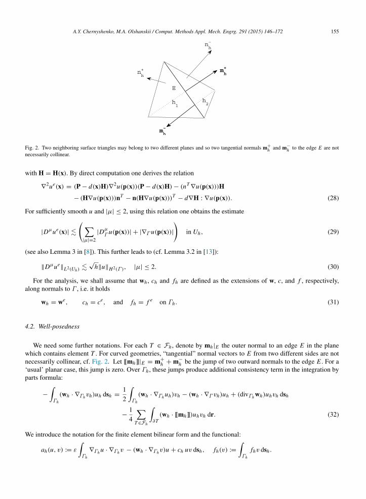
Fig. 2. Two neighboring surface triangles may belong to two different planes and so two tangential normals m+
h and m−
h to the edge E are notnecessarily collinear.
with H = H(x). By direct computation one derives the relation
∇2ue(x) = (P − d(x)H)∇2u(p(x))(P − d(x)H)− (nT
∇u(p(x)))H
− (H∇u(p(x)))nT− n(H∇u(p(x)))T − d∇H : ∇u(p(x)). (28)
For sufficiently smooth u and |µ| ≤ 2, using this relation one obtains the estimate
|Dµue(x)| .
|µ|=2
|Dµ
Γ u(p(x))| + |∇Γ u(p(x))|
in Uh, (29)
(see also Lemma 3 in [8]). This further leads to (cf. Lemma 3.2 in [13]):
∥Dµue∥L2(Uh)
.√
h∥u∥H2(Γ ), |µ| ≤ 2. (30)
For the analysis, we shall assume that wh , ch and fh are defined as the extensions of w, c, and f , respectively,along normals to Γ , i.e. it holds
wh = we, ch = ce, and fh = f e on Γh . (31)
4.2. Well-posedness
We need some further notations. For each T ∈ Fh , denote by mh |E the outer normal to an edge E in the planewhich contains element T . For curved geometries, “tangential” normal vectors to E from two different sides are notnecessarily collinear, cf. Fig. 2. Let [[mh]]|E = m+
h + m−
h be the jump of two outward normals to the edge E . For a‘usual’ planar case, this jump is zero. Over Γh , these jumps produce additional consistency term in the integration byparts formula:
−
Γh
(wh · ∇Γhvh)uh dsh =12
Γh
(wh · ∇Γh uh)vh − (wh · ∇Γ vh)uh + (divΓh wh)uhvh dsh
−14
T ∈Fh
∂T(wh · [[mh]])uhvh dr. (32)
We introduce the notation for the finite element bilinear form and the functional:
ah(u, v) := ε
Γh
∇Γh u · ∇Γhv − (wh · ∇Γhv)u + ch uv dsh, fh(v) :=
Γh
fhv dsh .

156 A.Y. Chernyshenko, M.A. Olshanskii / Comput. Methods Appl. Mech. Engrg. 291 (2015) 146–172
The following result is now straightforward.
Proposition 4.1. If one assumesΓh
ch +
12
divΓh wh
v2
h dsh −14
T ∈Fh
∂T(wh · [[mh]])v2
h dr ≥ c0∥vh∥2L2(Γh)
, for all vh ∈ V Γh , (33)
then the bilinear form is positive-definite on V Γh and so the trace finite element method (14) is well-posed. The solution
uh satisfies the a priori estimate,
c0
2∥uh∥
2L2(Γh)
+ ε∥∇Γh u∥2L2(Γh)
≤ c−10 ∥ f ∥
2L2(Γh)
. (34)
If ch = 0 and wh = 0 on Γh (the Laplace–Beltrami problem), then one imposes the zero mean conditions forthe solution and the right-hand side
Γh
fh =Γh
uh = 0 and proves the well-posedness result with the help of thePoincare inequality on Γh . For the mesh sufficiently fine, the Poincare constant is uniformly bounded independent ofh, see Lemma 4.1 in [26].
To assess how restrictive the assumption in (33), we invoke the following estimates (Lemmas 3.5 and 3.6 in [23])to bound the edge terms:
|P(x)[[mh]](x)| . h2 for x ∈ E,
and T ∈Fh
∂Tv2
h dsh . h−1∥vh∥
2L2(Γh)
+ h∥∇Γhvh∥2L2(Γh)
for all vh ∈ V Γh .
We remark that in [23] these estimates were proved for tetrahedra bulk subdivision, but all arguments carry over tocubic bulk meshes once we assume that the number of refinement level in octree is bounded. Since Pwe
= we, we getwith wh = we on Γh :
T ∈Fh
∂T(wh · [[mh]])v2
h dr
. h∥vh∥2L2(Γh)
+ h3∥∇Γhvh∥
2L2(Γh)
.
Therefore, we conclude that for sufficiently fine mesh, the bilinear form ah is positive definite on V Γh and so the
discrete problem is well-posed under condition similar to the differential case: ch +12 divΓh wh ≥ c0 > 0 on Γh .
4.3. Consistency estimate
The consistency error of the finite element method (14) is due to geometric errors resulting from the approximationof Γ by Γh . To estimate these geometric errors, we need a few additional definitions and results, which can be foundin, for example, [38]. For x ∈ Γh define Ph(x) = I−nh(x)n(x)T /(nh(x)·n(x)). One can represent the surface gradientof u ∈ H1(Γ ) in terms of ∇Γh ue as follows
∇Γ u(p(x)) = (I − d(x)H(x))−1Ph(x)∇Γh ue(x) a.e. x ∈ Γh .
Due to (24), we getΓ
∇Γ u∇Γ v ds =
Γh
Ah∇Γh ue∇Γhv
e dsh for all v ∈ H1(Γ ),
with Ah(x) = µh(x)PTh (x)(I − d(x)H(x))−2Ph(x). From w · n = 0 on Γ and we(x) = w(p(x)), n(x) = n(p(x)) it
follows that n(x) · we(x) = 0 and thus w(p(x)) = Ph(x)we(x) holds. Using this, we get the relationΓ(w · ∇Γ u)v ds =
Γh
(Bhwe· ∇Γh ue)ve dsh,

A.Y. Chernyshenko, M.A. Olshanskii / Comput. Methods Appl. Mech. Engrg. 291 (2015) 146–172 157
with Bh = µh(x)PTh (I − dH)−1Ph . We shall use the lifting procedure Γh → Γ given by
vlh(p(x)) := vh(x) for x ∈ Γh .
It is easy to see that vlh ∈ H1(Γ ).
The following lemma estimates the consistency error of the finite element method (14).
Lemma 4.1. Let u ∈ H2(Γ ) be the solution of (5) and assume (31), then we have
supvh∈V Γ
h
| fh(vh)− ah(ue, vh)|
∥vh∥H1(Γh)
. h2(∥u∥H1(Γ ) + ∥ f ∥L2(Γ )).
Proof. The residual is decomposed as
fh(vh)− ah(ue, vh) = fh(vh)− f (vl
h)+ a(u, vlh)− ah(u
e, vh). (35)
The following holds:
f (vlh) =
Γ
f vlh ds =
Γh
µh f evh dsh,
a(u, vlh) = ε
Γ
∇Γ u∇Γ vlh ds −
Γ(w · ∇Γ v
lh)u ds +
Γ
c uvlh ds
= ε
Γh
Ah∇Γh ue∇Γhvh dsh −
Γh
(Bhwe· ∇Γhvh)u
e dsh +
Γh
µhceuevh dsh .
Substituting these relations into (35) results in
fh(vh)− ah(ue, vh) =
Γh
(1 − µh) f evh dsh + ε
Γh
(Ah − Ph)∇Γh ue· ∇Γhvh dsh
−
Γh
((Bh − Ph)we· ∇Γhvh)u
e dsh +
Γh
(µh − 1)ceuevh dsh =: I1 + I2 + I3 + I4. (36)
We estimate the Ii terms separately. Applying (25) we obtain
I1 + I4 . h2∥ f e
∥L2(Γh)∥vh∥L2(Γh)
. (37)
One can show, cf. (3.43) in [13], the bound
|Ph − Ah | = |Ph(I − Ah)| . h2.
Using this and (27) we obtain
I2 . h2∥∇Γh ue
∥L2(Γh)∥∇Γhvh∥L2(Γh)
. h2∥ue
∥H1(Γ )∥vh∥H1(Γh). (38)
Since (I − dH)−1= I + O(h2), we also estimate
|Bh − Ph | . h2+ |Ah − Ph | . h2.
This yields
I3 . h2∥∇Γhvh∥L2(Γh)
∥ue∥L2(Γh)
. h2∥u∥H1(Γ )∥vh∥H1(Γh)
. (39)
Combining the results (36)–(39) proves the lemma.
4.4. Interpolation bounds
For a smooth function v defined on Γ consider its extension on Γh , ve. In this subsection, we show that ve can beapproximated using the finite element trace space V Γ
h with optimal order accuracy. First we need the following simplelemma.

158 A.Y. Chernyshenko, M.A. Olshanskii / Comput. Methods Appl. Mech. Engrg. 291 (2015) 146–172
Lemma 4.2. Consider an arbitrary plane P ⊂ R3 and any cubic cell S ∈ Th . It holds
∥v∥2L2(S∩P) . h−1
S ∥v∥2L2(S) + hS∥∇v∥2
L2(S) ∀ v ∈ H1(S). (40)
Proof. The proof follows from the fact that any cubic cell is divided into a finite number of regular tetrahedra andfurther applying Lemma 4.2 from [39] on each of these tetrahedra.
Now we are ready to prove the trace finite element interpolation bounds.
Theorem 4.1. For arbitrary v ∈ H2(Γ ) the following estimate holds with a constant c independent of h, v, and onhow Γh intersects Th:
infvh∈V Γ
h
∥ve
− vh∥L2(Γh)+ h∥∇Γh (v
e− vh)∥L2(Γh)
≤ ch2
∥v∥H2(Γ ). (41)
Proof. Assume the maximum cell size h in Th is attained at level k of the octree. Then the cells at the level k provideuniform cartesian subdivision which covers Ω . Denote this subdivision by T k
h and the set of corresponding nodes byN k
h . Note that v ∈ H2(Γ ) and Γ ∈ C2 imply ve∈ H2(Uh) for the normal extension and we may define the nodal
piecewise trilinear interpolant Ih(ve) such that Ih(v
e)(x) = ve(x) for x ∈ N kh ∩ Uh and Ih(v
e)(x) = 0 in other nodes.Since T k
h does not contain hanging nodes, Ih(ve) is continuous and so it holds Ih(v
e) ∈ Vh .Using the result in (40) and the interpolation properties of Ih(v
e), we get for vh = Ih(ve)|Γh :
∥ve− vh∥
2L2(Γh)
+ h2∥∇Γh (v
e− vh)∥
2L2(Γh)
=
T ∈Fh
∥ve− vh∥
2L2(T ) + h2
∥∇Γh (ve− vh)∥
2L2(T )
≤
T ∈Fh
h−1ST
∥ve− Ih(v
e)∥2L2(ST )
+ h2h−1ST
∥∇(ve− Ih(v
e))∥2L2(ST )
+ h3∥∇
2(ve− Ih(v
e))∥2L2(ST )
≤ C h4h−1ST
T ∈Fh
∥ve∥
2H2(ST )
.
The assumption that the number of local refinement levels is bounded yields hh−1ST
≤ C . Hence, it holds
∥ve− vh∥
2L2(Γh)
+ h2∥∇Γh (v
e− vh)∥
2L2(Γh)
≤ h3∥ve
∥2H2(Uh)
.
It remains to apply (30).
4.5. Error estimates
Now we combine the results derived in the previous sections to prove the first error estimate.
Theorem 4.2. Assume u is the solution of (5) and let uh be the discrete solution of the trace finite element method (14).Then the following estimate holds:
∥ue− uh∥H1(Γh)
. h∥ f ∥L2(Γ ). (42)
Proof. Consider an interpolant (Ihue) ∈ Vh from Theorem 4.1. The triangle inequality yields
∥ue− uh∥H1(Γh)
≤ ∥ue− (Ihue)|Γh ∥H1(Γh)
+ ∥(Ihue)|Γh − uh∥H1(Γh). (43)
The second term in the upper bound can be estimated using coercivity, continuity of the finite element bilinear form,interpolation properties from Theorem 4.1, and the consistency estimate in Lemma 4.1:
∥(Ihue)|Γh − uh∥2H1(Γh)
. ah((Ihue)|Γh − uh, (Ihue)|Γh − uh)
= ah((Ihue)|Γh − ue, (Ihue)|Γh − uh)+ ah(ue− uh, (Ihue)|Γh − uh)
. h∥u∥H2(Γ )∥(Ihue)|Γh − uh∥H1(Γh)+ |ah(u
e, (Ihue)|Γh − uh)− fh((Ihue)|Γh − uh)|
. h∥u∥H2(Γ ) + ∥ f ∥L2(Γ )
∥(Ihue)|Γh − uh∥H1(Γh)
.

A.Y. Chernyshenko, M.A. Olshanskii / Comput. Methods Appl. Mech. Engrg. 291 (2015) 146–172 159
This results in
∥(Ihue)|Γh − uh∥H1(Γh). h(∥u∥H2(Γ ) + ∥ f ∥L2(Γ )). (44)
The error estimate (42) follows from (43), (44), (41), and ∥u∥H2(Γ ) . ∥ f ∥L2(Γ ).
We now apply a duality argument to obtain an L2(Γh) error bound.
Theorem 4.3. Additionally assume that (9) and (33) hold with w replaced by −w. With the same u, uh as in Theo-rem 4.2, the following error bound holds
∥ue− uh∥L2(Γh)
. h2∥ f ∥L2(Γ ). (45)
Proof. Denote eh := (ue−uh)|Γh and let el
h be the lift of eh on Γ . Consider the problem: Find w ∈ H1(Γ ), such that
a(v,w) =
Γ
elhv ds for all v ∈ H1(Γ ). (46)
The problem is well-posed and the solution w satisfies w ∈ H2(Γ ) and ∥w∥H2(Γ ) . ∥elh∥L2(Γ ). Furthermore,
∥we∥H1(Γh)
. ∥w∥H1(Γ ) . ∥elh∥L2(Γ ). Due to (46) we have, for any ψh ∈ V Γ
h ,
∥elh∥
2L2(Γ ) = a(el
h, w) = a(elh, w)− ah(eh, w
e)+ ah(eh, we− ψh)+ ah(eh, ψh)
=
a(el
h, w)− ah(eh, we)
+ ah(eh, we− ψh)+
ah(u
e, ψh)− fh(ψh). (47)
We let ψh = (Ihue) ∈ Vh , interpolant given by Theorem 4.1. The terms on the right hand side of (47) are treatedseparately. The bound for the third one follows from Lemma 4.1:
ah(ue, ψh)− fh(ψh) . h2(∥u∥H1(Γ ) + ∥ f ∥L2(Γ ))∥ψh∥H1(Γh)
. h2(∥u∥H1(Γ ) + ∥ f ∥L2(Γ ))∥ue∥H2(Γ ). (48)
The bound for the second term follows from the continuity of the bilinear form, interpolation properties in Theorem 4.1and the error bound in Theorem 4.2:
ah(eh, we− ψh) . ∥eh∥H1(Γh)
∥we− ψh∥H1(Γh)
. h2∥ f ∥L2(Γ )∥w
e∥H2(Γ ). (49)
For the first term we get the expression similar to (36):
a(elh, w)− ah(eh, w
e) = ε
Γh
(Ah − Ph)∇Γhwe· ∇Γh eh dsh
−
Γh
((Bh − Ph)we· ∇Γhw
e)eh dsh +
Γh
(µh − 1)ceweeh dsh .
Hence, repeating the same argument as in the proof of Lemma 4.1, we get
a(elh, w)− ah(eh, w
e) . h2∥eh∥H1(Γh)
∥we∥H1(Γ ).
Further, employing the error bound from Theorem 4.2, we have
a(elh, w)− ah(eh, w
e) . h3∥ f ∥L2(Γ )∥w
e∥H1(Γ ). (50)
Combining (47)–(50) with the regularity result for the solution of the dual problem (46) completes the proof.
4.6. A posteriori estimate and error indicator
In this section, we deduce an a posteriori error estimate for the trace FEM. Based on this estimate we define aresidual type error indicator, which we use for a mesh adaptation purpose. We will treat only the formulation withsurface gradient (14) and assume that the Peclet number is sufficiently small and hence no additional stabilization isneeded.
160 A.Y. Chernyshenko, M.A. Olshanskii / Comput. Methods Appl. Mech. Engrg. 291 (2015) 146–172
Consider the surface finite element error eh = ue− uh on Γh . We prove an a posteriori bound for the lift of eh on
Γ , i.e. elh = u − ul
h on Γ . Thanks to (9) the functional ∥[v]∥ := (ε∥∇Γ v∥2L2(Γ )
+ ∥(c +12 divΓ w) v∥2
L2(Γ ))
12 defines a
norm on V such that
∥[elh]∥ ≤ sup
ψ : ∥[ψ]∥=1
Γ
a(elh, ψ) ds. (51)
Now we let ψ ∈ V with ∥[ψ]∥ = 1. For arbitrary ψh ∈ Vh , observe the identities
a(elh, ψ) =
Γ
fψ ds − a(ulh, ψ)
=
Γh
f eµh(ψe− ψh) dsh +
Γh
( f eµh − f e)ψh dsh + ah(uh, ψh)− a(ulh, ψ)
=
Γh
f eµh(ψe− ψh) dsh +
Γh
f e(µh − 1)ψh dsh + ah(uh, ψh − ψe)
−
ε
Γh
(Ah − Ph)∇Γh uh · ∇Γhψe dsh −
12
Γh
((Bh − Ph)we· ∇Γhψ
e)uh dsh
+
Γh
(µh − 1)ceuhψe dsh
. (52)
We apply elementwise integration by parts to the third term on the right hand side of (52):
ah(uh, ψh − ψe) =
Γh
(ε∆Γh uh − (ch + divΓh wh)uh − wh · ∇Γh uh)(ψe− ψh) dsh
−12
T ∈Fh
∂Tε[[∇Γh uh]](ψe
− ψh) dr +12
T ∈Fh
∂T(wh · [[mh]])uh(ψ
e− ψh) dr, (53)
where [[∇Γh uh]] denotes the jump in the normal derivative across an edge of T . Substituting (53) into (52) and applyingthe Cauchy inequality elementwise over Fh , we get
a(elh, ψ) .
T ∈Fh
|1 − µh |2L∞(T )
∥ f e
∥2L2(T ) + ∥uh∥
2L2(T )
+ ∥Ah − Ph∥
2L∞(T )∥∇Γh uh∥
2L2(T )
+ ∥Bh − Ph∥2L∞(T )∥uh∥
2L2(T )
12
∥ψe∥H1(Γh)
+
T ∈Fh
ηR(T )
2+ ηE (T )
2 1
2
×
T ∈Fh
h−2
ST∥ψe
− ψh∥2L2(T ) +
e∈∂T
h−1ST
∥ψe− ψh∥
2L2(e)
12
, (54)
with
ηR(T )2
= h2ST
∥ fh + ε∆Γh uh − (ch + divΓh wh)uh − wh · ∇Γh uh∥2L2(T )
ηE (T )2
=
e∈∂T
hST
∥[[ε∇Γh uh]]∥
2L2(e) + ∥wh · [[mh]]∥
2L2(e)
.
Combining (51) and (54) leads to an a posteriori error estimate, where ψ-dependent terms on the right hand sideshould be handled further. Due to (24) and (27) we have
∥ψe∥H1(Γh)
. ∥ψ∥H1(Γ ). (55)
For every e ∈ ∂T denote by Te ⊂ ST a plane segment of the regular shape such that diam(Te) ≃ hST . We apply theresult in (40) and its two-dimensional analog to estimate

A.Y. Chernyshenko, M.A. Olshanskii / Comput. Methods Appl. Mech. Engrg. 291 (2015) 146–172 161
h−2ST
∥ψe− ψh∥
2L2(T ) +
e∈∂T
h−1ST
∥ψe− ψh∥
2L2(e)
. h−3ST
∥ψe− ψh∥
2L2(ST )
+ h−1ST
∥∇(ψe− ψh)∥
2L2(ST )
+
e∈∂T
h−2
ST∥ψe
− ψh∥2L2(Te)
+ ∥∇(ψe− ψh)∥
2L2(Te)
. h−3
ST∥ψe
− ψh∥2L2(ST )
+ h−1ST
∥∇(ψe− ψh)∥
2L2(ST )
+
e∈∂T
∥∇ψe
∥2L2(Te)
+ ∥∇ψh∥2L2(Te)
. h−3
ST∥ψe
− ψh∥2L2(ST )
+ h−1ST
∥∇(ψe− ψh)∥
2L2(ST )
+
∥∇Γψ∥
2L2(p(ST ))
+ h−1ST
∥∇ψh∥2L2(ST )
. (56)
In this paper we consider only graded octree meshes. In terms of [40], these are 1-irregular meshes and hence forψe
∈ H1(Ω) (assuming arbitrary smooth extension of ψe from Uh to Ω ) one can consider a Scott–Zhang typeinterpolant ψh ∈ Vh such that
h−1S ∥ψe
− ψh∥L2(S) + ∥∇ψh∥L2(S) . ∥ψe∥H1(ω(S)) ∀ S ∈ Ωh, (57)
where ω(S) is defined as follows: Let ω(S) consist of S and of all cubic cells touching S, then ω(S) is a patch of cellsdefined as the union of ω(S) and of all cubic cells touching ω(S). We assume c in (20) to be sufficiently large and hsufficiently small that ω(S) ⊂ Uh for all S ∈ Ωh . Applying (57) in (56) yields
T ∈Fh
h−2
ST∥ψe
− ψh∥2L2(T ) +
e∈∂T
h−1ST
∥ψe− ψh∥
2L2(e)
.
T ∈Fh
h−1
ST∥ψe
∥2H1(ω(ST ))
+ ∥∇Γψ∥2L2(p(ST ))
.
T ∈Fh
∥ψ∥2H1(p(ω(ST )))
≃
S∈Ωh
∥ψ∥2H1(p(ω(S))). (58)
In the last inequality we used the fact that for the graded octree mesh diam(ω(ST )) ≃ hST . For any two patches ω(S1)
and ω(S2), S1, S2 ∈ Ωh , the number of cubic cells in ω(S1) ∩ ω(S2) is bounded by a constant independent of h andthe number of refinement levels. However, for the projections on Γ the intersection p(ω(S1)) ∩ p(ω(S2)) may benonempty, even if two patches do not overlap. Thus x ∈ Γ may belong to the projections of patches for several cellsin Ωh , but the number of such patches may not grow faster than O(K ) uniformly over Γ , where K is the number ofthe levels in the octree. Therefore it holds
T ∈Fh
∥ψ∥2H1(p(ω(ST )))
. K∥ψ∥2H1(Γ ). (59)
We assumed that the number of levels is uniformly bounded for the family of meshes and so K = O(1), while ingeneral case it holds K . | ln hmin|. Using (56)–(59), we prove the existence of ψh ∈ Vh such that
T ∈Fh
h−2
ST∥ψe
− ψh∥2L2(T ) +
e∈∂T
h−1ST
∥ψe− ψh∥
2L2(e)
. ∥ψ∥
2H1(Γ ). (60)
Combining (51) and (55), (60) gives the following a posteriori error estimate
∥[elh]∥ .
T ∈Fh
|1 − µh |2L∞(T )
∥ f e
∥2L2(T ) + ∥uh∥
2L2(T )
+ ∥Ah − Ph∥
2L∞(T )∥∇Γh uh∥
2L2(T )
+ ∥Bh − Ph∥2L∞(T )∥uh∥
2L2(T )
12
+
T ∈Fh
ηR(T )
2+ ηE (T )
2 1
2
. (61)
Finally, if we assume that local grid refinement leads to better local surface reconstruction, i.e. (22) and (23)can be formulated locally, then the first term on the right-hand side of (61) is of higher order. We may assume|1−µh |
2L∞(T )+∥Ah −Ph∥
2L∞(T )+∥Bh −Ph∥
2L∞(T ) . h4
ST∥H∥
2L∞(p(T )). This suggests introducing also the geometric

162 A.Y. Chernyshenko, M.A. Olshanskii / Comput. Methods Appl. Mech. Engrg. 291 (2015) 146–172
error indicator
ηG(T )2
:= h4ST
∥Hh∥2L∞(T )
∥ f e
∥2L2(T ) + ∥uh∥
2H1(T )
,
where Hh is a Hessian reconstruction on Γh .Thus, for the purpose of local mesh adaptation we use the following error indicator:
η(T ) := (αrηR(T )2+ αeηE (T )
2+ αgηG(T )
2)12 (62)
with some parameters αr , αe, αg ≥ 0. We set αg equal to 0 or 1 depending on whether we wish to account (explicitly)for geometric errors or not. For regular elliptic problems we set αr = αe = 1, while for transport dominated problemsmore weight is put on the edge error indicator (see next section). We also note that the second edge term in thedefinition of ηE (T )2 is of higher order. Our numerical experience suggests that it can be excluded without any notablechange in the performance of an adaptive method.
Results of experiments in the next section show that the trace FE adaptive method based on η(T ) and standard“maximum” marking strategy leads to optimal convergence of the error in H1 and L2 norms.
5. Numerical examples
5.1. Smooth solutions on a sphere and a torus
Example 1. As a first test problem we consider the Laplace–Beltrami type equation on the unit sphere:
−∆Γ u + u = f on Γ ,
with Γ = x ∈ R3| ∥x∥2 = 1 and Ω = (−2, 2)3. The source term f is taken such that the solution is given by
u(x) =a
∥x∥3
3x2
1 x2 − x32
, x = (x1, x2, x3) ∈ Ω ,
with a = 12. Using the representation of u in spherical coordinates one can verify that u is an eigenfunction of −∆Γ :u(r, φ, θ) = a sin(3φ) sin3 θ , −∆Γ u + u = 13u =: f (r, φ, θ). Both u and f are constant along normals at Γ .
Example 2. In the second example, we consider a torus instead of the unit sphere and the same equation: Γ ⊂ Ω =
(−2, 2)3, with Γ = x ∈ Ω | r2= x2
3 + (
x2
1 + x22 − R)2. We take R = 1 and r = 0.6. In the coordinate system
(ρ, φ, θ), with
x = R
cosφsinφ
0
+ ρ
cosφ cos θsinφ cos θ
sin θ
,the ρ-direction is normal to Γ , ∂x
∂ρ⊥ Γ for x ∈ Γ . Thus, the following solution u and corresponding right-hand side
f are constant in the normal direction:
u(x) = sin(3φ) cos(3θ + φ),
f (x) = r−2(9 sin(3φ) cos(3θ + φ))− (R + r cos(θ))−2(−10 sin(3φ) cos(3θ + φ)− 6 cos(3φ) sin(3θ + φ))
− r(R + r cos(θ))−1(3 sin(θ) sin(3φ) sin(3θ + φ))+ u(x). (63)
We compute numerical solutions to Examples 1 and 2 using the trace FE methods (14) and (16) on a sequence ofoctree bulk grids. The initial grid was uniform with h =
14 . Further the grid was gradely refined towards the surfaces.
All linear algebra systems in this and further experiments were solved with the help of PETSc library: We computedLU factorizations of diagonally scaled stiffness matrices. Finite element errors and convergence rates are shown inTable 1. Both variants demonstrate second order convergence in L2 surface norm and close to second order in L∞
surface norm. Computed solutions and final meshes are visualized in Fig. 3.
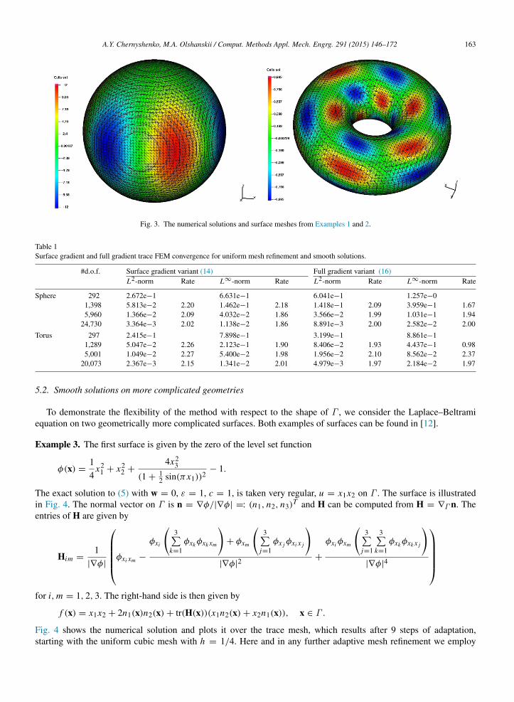
A.Y. Chernyshenko, M.A. Olshanskii / Comput. Methods Appl. Mech. Engrg. 291 (2015) 146–172 163
Fig. 3. The numerical solutions and surface meshes from Examples 1 and 2.
Table 1Surface gradient and full gradient trace FEM convergence for uniform mesh refinement and smooth solutions.
#d.o.f. Surface gradient variant (14) Full gradient variant (16)L2-norm Rate L∞-norm Rate L2-norm Rate L∞-norm Rate
Sphere 292 2.672e−1 6.631e−1 6.041e−1 1.257e−01,398 5.813e−2 2.20 1.462e−1 2.18 1.418e−1 2.09 3.959e−1 1.675,960 1.366e−2 2.09 4.032e−2 1.86 3.566e−2 1.99 1.031e−1 1.94
24,730 3.364e−3 2.02 1.138e−2 1.86 8.891e−3 2.00 2.582e−2 2.00
Torus 297 2.415e−1 7.898e−1 3.199e−1 8.861e−11,289 5.047e−2 2.26 2.123e−1 1.90 8.406e−2 1.93 4.437e−1 0.985,001 1.049e−2 2.27 5.400e−2 1.98 1.956e−2 2.10 8.562e−2 2.37
20,073 2.367e−3 2.15 1.341e−2 2.01 4.979e−3 1.97 2.184e−2 1.97
5.2. Smooth solutions on more complicated geometries
To demonstrate the flexibility of the method with respect to the shape of Γ , we consider the Laplace–Beltramiequation on two geometrically more complicated surfaces. Both examples of surfaces can be found in [12].
Example 3. The first surface is given by the zero of the level set function
φ(x) =14
x21 + x2
2 +4x2
3
(1 +12 sin(πx1))2
− 1.
The exact solution to (5) with w = 0, ε = 1, c = 1, is taken very regular, u = x1x2 on Γ . The surface is illustratedin Fig. 4. The normal vector on Γ is n = ∇φ/|∇φ| =: (n1, n2, n3)
T and H can be computed from H = ∇Γ n. Theentries of H are given by
Him =1
|∇φ|
φxi xm −
φxi
3
k=1φxkφxk xm
+ φxm
3
j=1φx jφxi x j
|∇φ|2
+
φxiφxm
3
j=1
3k=1
φxkφxk x j
|∇φ|4
for i,m = 1, 2, 3. The right-hand side is then given by
f (x) = x1x2 + 2n1(x)n2(x)+ tr(H(x))(x1n2(x)+ x2n1(x)), x ∈ Γ .
Fig. 4 shows the numerical solution and plots it over the trace mesh, which results after 9 steps of adaptation,starting with the uniform cubic mesh with h = 1/4. Here and in any further adaptive mesh refinement we employ

164 A.Y. Chernyshenko, M.A. Olshanskii / Comput. Methods Appl. Mech. Engrg. 291 (2015) 146–172
Fig. 4. Illustration of the surface and solution from Example 3. The right figure shows also triangulation after 7 steps of adaptation based on theerror indicator.
Fig. 5. Left: Adaptive trace FEM convergence in Example 3. Right: The zoom of the trace surface mesh in Example 3. The adaptation was basedon the residual indicator accounting for geometric errors.
a “maximum” marking strategy in which all volume cubes S from ωh with η(S) > 12 maxS∈ωh η(S) are marked for
further refinement. Note that some adjunct cubes also may need refinement if one wishes to keep the octree balanced.Fig. 5 (right) displays the finite element error reduction if the mesh adaptation process is based on the error indicator(62). The results demonstrate optimal convergence order of the adaptive trace FEM with respect to the total numberof degrees of freedom in L2, H1 and L∞ surface norms. The results are shown for the surface gradient variant ofthe method (14). Here and further “number of d.o.f.” means only the number of active degrees of freedom, which isequal to the dimension of the resulting system of linear algebraic equations. We set αg = 1 in the error indicator toaccount for geometric errors. The left plot in Fig. 5 zooms the trace surface mesh. From this plot we see that the meshrefinement generally happens in regions with higher surface curvatures.
Example 4. This is another example of a more complicated domain, which is homeomorphic to the sphere with 6handles, see Fig. 6. The surface is given implicitly as the zero level set of
φ = (x21 + x2
2 − 4)2 + (x22 − 1)2 + (x2
2 + x23 − 4)2 + (x2
1 − 1)2 + (x21 + x2
3 − 4)2 + (x23 − 1)2 − 13.
We solve the Laplace–Beltrami equation with right-hand side f = 1004
j=1 exp(−|x − x j|2), with
x1= (−1, 1, 2.04), x2
= (1, 2.04, 1), x3= (2.04, 0, 1), x4
= (−0.− 1,−2.04).
The points are close to the surface and the right-hand side is varying rapidly in vicinities of these 4 points, and hencethe same is expected from the solution. The solution and the grid resulted after 12 steps of refinement are visualizedin Fig. 6. The refinement was based on the error indicator (62) with αg = 1.

A.Y. Chernyshenko, M.A. Olshanskii / Comput. Methods Appl. Mech. Engrg. 291 (2015) 146–172 165
Fig. 6. The surface, numerical solution and adaptive mesh from Example 4.
5.3. Laplace–Beltrami problem with point singularity
Example 5. For the next test problem we consider the Laplace–Beltrami equation on the unit sphere. The solutionand the source term in spherical coordinates are given by
u = sinλ θ sinφ, f = (1 + λ2+ λ) sinλ θ sinφ + (1 − λ2) sinλ−2 θ sinφ. (64)
One verifies
∇Γ u = sinλ−1 θ
12
sin 2φ(λ cos2 θ − 1), sin2 φ(λ cos2 θ − 1)+ 1, −12λ sin 2θ sinφ
T
.
For λ < 1 the solution u is singular at the north and south poles of the sphere so that u ∈ H1(Γ ), but u ∈ H2(Γ ).Following [38] we set λ = 0.6 to model the point singularity and contrast it to the regular problem with λ = 1.
Results produced by the adaptive algorithm are shown in Fig. 7, where they are compared to the results for uniformgrid refinement. As expected, the regular refinement leads to a suboptimal convergence for the singular case ofλ = 0.6. Adaptive refinement driven by the error indicator (62) leads to optimal convergence rates in L2 and H1
surface norms. Note that reliability of the error indicator for H1 error norm was proved in [25] for tetrahedral meshes.A posteriori error analysis in other norms remains an open question.
The left column in Fig. 7 displays error decrease for the surface gradient formulation (14), while the right column ofplots displays error decrease for the full gradient formulation (16). Similar to regular problems and regular refinementin Examples 1 and 2, the adaptive algorithm shows close performance for both formulations producing slightly moreaccurate results for the surface gradient formulation (14).
Fig. 8 (left) displays a cutaway view which includes both the adaptively refined bulk and surface meshes. Themeshes are shown after the 12 refinement steps. The middle picture in Fig. 8 shows the surface mesh superimposedon numerical solution. The coarsest mesh is in the regions with the smallest solution gradient. Fig. 8 (right) displaysthe surface mesh near the north pole magnified 20 times. This local mesh appears more structured, since the surfaceis locally close to a plane which cuts through a regular bulk mesh.
5.4. Convection–diffusion problem with an internal layer
We now perform several tests for the advection–diffusion problem as in (5), with nonzero advection field w. Asusual, the properties of the problem essentially depend on the value of the dimensionless Peclet number. The Pecletnumber can be defined similar to volumetric case as Pe =
LW2ε , where L is a characteristic problem scale (say, the
diameter of a closed surface Γ ) and W is a characteristic advection velocity. For low values of the Peclet numbers, theproblem is close to the Laplace–Beltrami equation, while for higher Peclet numbers, the problem may demonstratebehavior typical to singular-perturbed equations, e.g., its solution may exhibit internal layers. The example considered

166 A.Y. Chernyshenko, M.A. Olshanskii / Comput. Methods Appl. Mech. Engrg. 291 (2015) 146–172
Fig. 7. Decrease of the error in H1(Γh)-norm (upper plots), L2(Γh)-norm (bottom plots) for the adaptive algorithm and Example 5. Left columnplots show results for the surface gradient formulation (14), while the right column plots show results for the full gradient formulation (16).
Fig. 8. Left and middle plots display the cutaway of the bulk and trace surface meshes in Example 5 with λ = 0.6 after 12 steps of refinement. Themiddle plot is shaded to reflect the numerical solution. The right picture shows the 20-x zoom in of the surface mesh near the north pole.
below is chosen to illustrate the ability of the trace FEM to handle these different cases by employing computationaltools developed for volumetric finite elements: stabilization, error indicators, and layer fitted meshes. Numerical

A.Y. Chernyshenko, M.A. Olshanskii / Comput. Methods Appl. Mech. Engrg. 291 (2015) 146–172 167
Fig. 9. Decrease of the error in the L2(Γ ), H1(Γ ) and L∞(Γ ) norms for the advection–diffusion problem from Example 6 with Pe = 1 (left)and Pe = 100 (right). The problem is solved on a sequence of adaptively refined grids.
results will show that the performance of such enhanced trace FEM appears to be similar to its volumetric counterpartsapplied to bulk advection–diffusion problems.
For the advection–diffusion problem we set weights αr , αe in the error indicator (62) dependent on the Pecletnumber as recommended in [41] for the planar advection–diffusion problem:
αr = minε−1, h−2ST
, αe = minε−1, h−1STε−
12 .
In experiments below geometry does not play an important role and so we set αg = 0.
Example 6. In this example, the stationary problem (5) is solved on the unit sphere Γ , with the velocity field
w(x) =
−x2
1 − x2
3 , x1
1 − x2
3 , 0T
,
which is tangential to the sphere. We set c = 1 and consider ε ∈ [10−6, 1]. Letting W := ∥w∥L∞(Γ ) and L = diam(Γ ),we compute the Peclet number as Pe = ε−1.
For the exact solution to (5), we take the function
u(x) = x1x2arctan
2x3√ε
.
The corresponding right-hand side function f is given by
f (x) =12ε3/2x1x2x3
ε + 4x23
+16ε3/2(1 − x2
3)x1x2x3
(ε + 4x23)
2+ (6εx1x2 +
x2
1 + x22(x
21 − x2
2))arctan
2x3√ε
+ u.
When ε gets smaller, a layer of the width O(ε12 ) is forming in u along the equator of the sphere (x3 = 0 ∩ Γ ). The
formation of characteristic internal layers of O(ε12 )-width is typical for advection–diffusion problems.
In this paper, we consider equations posed on closed surfaces, therefore we are not treating parabolic or exponentialboundary layers.
5.4.1. Lower Peclet number caseWe consider Eq. (5) for Pe ≤ 100 to be non-singular perturbed. Hence, for this case of lower Peclet numbers,
we expect the trace finite element to behave similar to the case of Laplace–Beltrami equations with smooth solution.We add no stabilization in this case and recover the expected O(h2) and O(h) convergence rates on a sequence ofuniformly refined grids in L2 and H2 surface norms, respectively (not shown). Fig. 9 shows the error reduction plotsfor Pe = 1 and Pe = 100 if a mesh adaptation is performed based on the error indicator (62). For Pe = 100, the errornorms are approximately one order bigger than for Pe = 1, but in both cases the convergence curves demonstrate
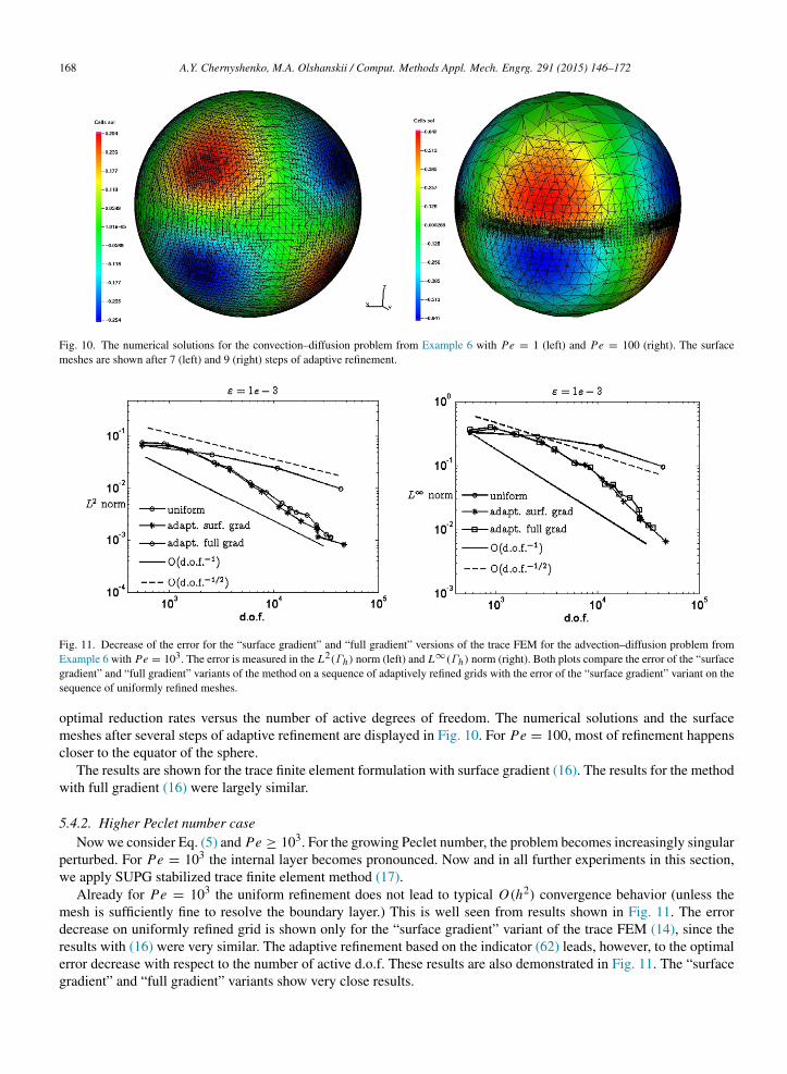
168 A.Y. Chernyshenko, M.A. Olshanskii / Comput. Methods Appl. Mech. Engrg. 291 (2015) 146–172
Fig. 10. The numerical solutions for the convection–diffusion problem from Example 6 with Pe = 1 (left) and Pe = 100 (right). The surfacemeshes are shown after 7 (left) and 9 (right) steps of adaptive refinement.
Fig. 11. Decrease of the error for the “surface gradient” and “full gradient” versions of the trace FEM for the advection–diffusion problem fromExample 6 with Pe = 103. The error is measured in the L2(Γh) norm (left) and L∞(Γh) norm (right). Both plots compare the error of the “surfacegradient” and “full gradient” variants of the method on a sequence of adaptively refined grids with the error of the “surface gradient” variant on thesequence of uniformly refined meshes.
optimal reduction rates versus the number of active degrees of freedom. The numerical solutions and the surfacemeshes after several steps of adaptive refinement are displayed in Fig. 10. For Pe = 100, most of refinement happenscloser to the equator of the sphere.
The results are shown for the trace finite element formulation with surface gradient (16). The results for the methodwith full gradient (16) were largely similar.
5.4.2. Higher Peclet number caseNow we consider Eq. (5) and Pe ≥ 103. For the growing Peclet number, the problem becomes increasingly singular
perturbed. For Pe = 103 the internal layer becomes pronounced. Now and in all further experiments in this section,we apply SUPG stabilized trace finite element method (17).
Already for Pe = 103 the uniform refinement does not lead to typical O(h2) convergence behavior (unless themesh is sufficiently fine to resolve the boundary layer.) This is well seen from results shown in Fig. 11. The errordecrease on uniformly refined grid is shown only for the “surface gradient” variant of the trace FEM (14), since theresults with (16) were very similar. The adaptive refinement based on the indicator (62) leads, however, to the optimalerror decrease with respect to the number of active d.o.f. These results are also demonstrated in Fig. 11. The “surfacegradient” and “full gradient” variants show very close results.

A.Y. Chernyshenko, M.A. Olshanskii / Comput. Methods Appl. Mech. Engrg. 291 (2015) 146–172 169
Fig. 12. Numerical solution and the mesh after 9 refinement steps for the convection–diffusion problem from Example 6 with Pe = 103.
Table 2
Convergence of numerical solutions to the advection–diffusion problem from Example 6, with Pe = 104, on a sequence of Shishkin meshes.
#d.o.f. L2-norm Rate H1-norm rate L∞-norm Rate
10,356 4.870e−3 1.577e−0 6.725e−222,830 1.428e−3 1.77 7.597e−1 1.05 1.718e−2 1.97
101,332 3.739e−4 1.93 3.761e−1 1.01 5.484e−3 1.65
The numerical solution computed after 9 refinement steps and the corresponding surface mesh are demonstrated inFig. 12. The internal characteristic layer is well seen in the solution. The error indicator (62) enforces an aggressiverefinement in the regions of the layer.
Further, we consider the same problem with the higher Peclet number equal to 104. This time, the adaptiverefinement based on the error indicator was not found to produce optimal error reduction for the number of degreesof freedom up to 50,000. Hence, we consider this problem to be a good test case for layer fitted meshes. We chooseShishkin meshes as one of the best studied class of meshes for singular-perturbed volumetric or planar problems.Shishkin meshes require an a priori knowledge of where a layer occurs and provide optimal convergence with respectto the total number of degrees of freedom [42].
Let N be the total number of nodal degrees of freedom available to discretize a singular-perturbed convection–diffusion problem. Assume that the solution to the problem has only an internal characteristic layer. Then to builda Shishkin mesh one defines a narrow band of width O(
√ε ln N ) around the layer and considers a mesh which is
uniform inside and outside the band and contains O(N ) nodes in the interior of the narrow band as well as in the restof computational domain (see, e.g., [42] for accurate definitions). We extend this construction to the case of octreebulk meshes and the singular-perturbed problem posed on a surface as follows. We build an initial octree mesh suchthat hmin = 1/128 was the size of cubes inside the strip |x3| ≤ 1/64 (this defines our “narrow band” containing thelayer). In the rest of the bulk domain, the grid was aggressively coarsened up to hmax = 1/4. The resulted number ofactive degrees of freedom for this initial mesh was 10,356. Further, the mesh was uniformly refined two times, leadingto layer fitted meshes with 22,830 and 101,332 active degrees of freedom. We note two deviations of our constructionfrom the classical notion of a Shishkin mesh: (i) We do not re-balance the mesh to account for the logarithmic factorin the width of a narrow band of a canonical Shishkin mesh; (ii) The mesh outside our narrow band is not completelyuniform due to a transition region, which is necessary to keep the octree balanced (two neighboring cubes may differin size at most by a factor of 2).
Fig. 13 shows the numerical solution computed on the finest surface Shishkin mesh. Note that the internal layer issharp and resolved. We observe no numerical oscillations in a vicinity of the layer. Table 2 presents the norms of thefinite element error on the sequence of the layer fitted meshes and corresponding convergence factors.

170 A.Y. Chernyshenko, M.A. Olshanskii / Comput. Methods Appl. Mech. Engrg. 291 (2015) 146–172
Fig. 13. Numerical solution and the Shishkin mesh for the advection–diffusion problem from Example 6 with the Pe = 104.
Fig. 14. Left: Decrease of the error in the L2(Γext), H1(Γext) and L∞(Γext) norms for the advection–diffusion problem from Example 6 withPe = 106. Γext is a part of the domain well separated from the internal layer. The problem was solved on a sequence of uniformly refined meshes.Right: Numerical solution for the advection–diffusion problem from Example 6 with Pe = 106 on a uniformly refined mesh. The internal layer isnot resolved and clearly smeared over few mesh sizes. No spurious oscillations can be noted.
Finally, we solve the same problem, but now with ε = 10−6, leading to Pe = 106. The width of the internal
layer is O(ε12 ), and we are not attempting to resolve it with a layer fitted mesh. Instead we solve the problem on a
sequence of uniformly refined grids. Since we used the SUPG stabilized formulation of the finite element method, wecan expect that similar to a planar or a volumetric cases the layer would be smeared, numerical oscillation damped,and finite element solution converges to the exact one outside the layer. This is exactly what we observed for our tracefinite element method. Thus, Fig. 14 demonstrates the computed solution as well as the finite element error decreasein a part of the domain separated from the layer: All norms in Fig. 14 (left) were computed over part of the sphereΓext := x ∈ Γ : |x3| > 0.3.
6. Conclusions
We studied a trace finite element method for partial differential equations posed on hypersurfaces in R3. Anextension to curves in R2 is straightforward. The paper demonstrates that using such standard computational toolsas cartesian octree grids, a marching cubes method, and trilinear bulk finite elements leads to a second order accuratemethod with a number of attractive features: The mesh is unfitted to a surface; One uses standard finite element toolswithout any extension of equation from the surface to bulk domain; The method works for surfaces defined implicitly,parametrization of a surface is not required; The number of active d.o.f. is optimal and comparable to methods in

A.Y. Chernyshenko, M.A. Olshanskii / Comput. Methods Appl. Mech. Engrg. 291 (2015) 146–172 171
which Γ is meshed directly; Optimal order of convergence in H1 and L2 norms is proved for quasi-uniform bulkgrids. Moreover, due to the natural connection to bulk elements, many tools and techniques well established for“usual” discretizations carry over to the surface case. In this paper, we experimented with several such techniques:adaptivity based on an error indicator, SUPG stabilization for transport dominant equations, and layer fitted meshes.Numerical analysis supports experimental observations. In forthcoming papers we plan to extend the adaptive octreetrace finite element method to PDEs defined on evolving surfaces and to apply it for the simulation of flow andtransport in fractured porous media.
Acknowledgments
This work has been supported by RFBR through the grants 14-01-00731, 14-01-00830 and by National ScienceFoundation through the Division of Mathematical Sciences grant 1315993.
References
[1] W.W. Mullins, Mass transport at interfaces in single component system, Metall. Mater. Trans. 26 (1995) 1917–1925.[2] C.M. Elliott, B. Stinner, Modeling and computation of two phase geometric biomembranes using surface finite elements, J. Comput. Phys.
229 (2010) 6585–6612.[3] S. Gross, A. Reusken, Numerical Methods for Two-phase Incompressible Flows, vol. 40, Springer-Verlag, 2011.[4] U. Diewald, T. Preufer, M. Rumpf, Anisotropic diffusion in vector field visualization on Euclidean domains and surfaces, IEEE Trans. Vis.
Comput. Graph. 6 (2000) 139–149.[5] G. Turk, Generating textures on arbitrary surfaces using reaction–diffusion, Comput. Graph. 25 (1991) 289–298.[6] A. Toga, Brain Warping, Academic Press, New York, 1998.[7] D. Halpern, O. Jensen, J. Grotberg, A theoretical study of surfactant and liquid delivery into the lung, J. Appl. Physiol. 85 (1998) 333–352.[8] G. Dziuk, Finite elements for the Beltrami operator on arbitrary surfaces, in: S. Hildebrandt, R. Leis (Eds.), Partial Differential Equations and
Calculus of Variations, in: Lecture Notes in Mathematics, vol. 1357, Springer, Berlin, 1988, pp. 142–155.[9] M. Bertalmio, L. Cheng, S. Osher, G. Sapiro, Variational problems and partial differential equations on implicit surfaces: The framework and
examples in image processing and pattern formation, J. Comput. Phys. 174 (2001) 759–780.[10] K. Deckelnick, C.M. Elliott, T. Ranner, Unfitted finite element methods using bulk meshes for surface partial differential equations, arXiv
preprint arXiv:1312.2905.[11] M. Olshanskii, D. Safin, A narrow-band unfitted finite element method for elliptic pdes posed on surfaces, arXiv preprint arXiv:1401.7697
Math. Comp., in press.[12] G. Dziuk, C.M. Elliott, Finite element methods for surface PDEs, Acta Numer. (2013) 289–396.[13] M. Olshanskii, A. Reusken, J. Grande, A finite element method for elliptic equations on surfaces, SIAM J. Numer. Anal. 47 (2009) 3339–3358.[14] M. Olshanskii, A. Reusken, A finite element method for surface PDEs: Matrix properties, Numer. Math. 114 (2010) 491–520.[15] A. Bonito, R. Nochetto, M. Pauletti, Dynamics of biomembranes: effect of the bulk fluid, Math. Model. Nat. Phenom. 6 (2011) 25–43.[16] C.M. Elliott, T. Ranner, Finite element analysis for coupled bulk-surface partial differential equation, IMA J. Numer. Anal. 33 (2013) 377–402.[17] J. Grande, Eulerian finite element methods for parabolic equations on moving surfaces, SIAM J. Sci. Comput. 36 (2014) 248–271.[18] P. Hansbo, M.G. Larson, S. Zahedi, Characteristic Cut Finite Element Methods for Convection–Diffusion Problems on Time Dependent
Surfaces, Tech. Rep., Uppsala University, 2013, April.[19] M. Olshanskii, A. Reusken, X. Xu, An eulerian space–time finite element method for diffusion problems on evolving surfaces, SIAM J.
Numer. Anal. 52 (2014) 1354–1377.[20] M. Olshanskii, A. Reusken, Error analysis of a space–time finite element method for solving PDEs on evolving surfaces, SIAM J. Numer.
Anal. 52 (2014) 2092–2120.[21] E. Burman, P. Hansbo, M.G. Larson, S. Zahedi, Cut finite element methods for coupled bulk-surface problems, arXiv preprint
arXiv:1403.6580.[22] S. Gross, M.A. Olshanskii, A. Reusken, A trace finite element method for a class of coupled bulk-interface transport problems, arXiv preprint
arXiv:1406.7694.[23] M. Olshanskii, A. Reusken, X. Xu, A stabilized finite element method for advection–diffusion equations on surfaces, IMA J Numer. Anal. 34
(2014) 732–758.[24] A. Reusken, Analysis of trace finite element methods for surface partial differential equations, IGPM RWTH Aachen preprint 387.[25] A. Demlow, M. Olshanskii, An adaptive surface finite element method based on volume meshes, SIAM J. Numer. Anal. 50 (2012) 1624–1647.[26] E. Burman, P. Hansbo, M.G. Larson, A stabilized cut finite element method for partial differential equations on surfaces: The Laplace–Beltrami
operator, Comput. Methods Appl. Mech. Engrg. 285 (2015) 188–207.[27] F. Losasso, F. Gibou, R. Fedkiw, Simulating water and smoke with an octree data structure, ACM Trans. Graph. (TOG) 23 (3) (2004) 495–514.[28] D. Meagher, Geometric modeling using octree encoding, Comput. Graph. Image Process. 19 (1982) 129–147.[29] R. Szeliski, Rapid octree construction from image sequences, CVGIP: Image Underst. 58 (1993) 23–32.[30] S. Popinet, An accurate adaptive solver for surface-tension-driven interfacial flows, J. Comput. Phys. 228 (2009) 5838–5866.[31] J. Strain, Tree methods for moving interfaces, J. Comput. Phys. 151 (1999) 616–648.[32] K.D. Nikitin, M.A. Olshanskii, K.M. Terekhov, Y.V. Vassilevski, A numerical method for the simulation of free surface flows of viscoplastic
fluid in 3D, J. Comput. Math. 29 (2011) 605–622.

172 A.Y. Chernyshenko, M.A. Olshanskii / Comput. Methods Appl. Mech. Engrg. 291 (2015) 146–172
[33] W. Bangerth, R. Hartmann, G. Kanschat, DEAL II – a general-purpose object-oriented finite element library, ACM Trans. Math. Software(TOMS) 33 (4).
[34] S. Popinet, Gerris: a tree-based adaptive solver for the incompressible Euler equations in complex geometries, J. Comput. Phys. 190 (2003)572–600.
[35] W. Lorensen, H. Cline, Marching cubes: A high resolution 3d surface construction algorithm, ACM SIGGRAPH 21 (4) (1987) 189–207.[36] T. Aubin, Nonlinear Analysis on Manifolds, Monge–Ampere Equations, Vol. 252, Springer, 1982.[37] C.-C. Ho, F.-C. Wu, B.-Y. Chen, Y.-Y. Chuang, M. Ouhyoung, Cubical marching squares: Adaptive feature preserving surface extraction from
volume data, in: EUROGRAPHICS 2005 / M. Alexa and J. Marks (Guest Editors) 24 (3).[38] A. Demlow, G. Dziuk, An adaptive finite element method for the Laplace–Beltrami operator on implicitly defined surfaces, SIAM J. Numer.
Anal. 45 (2007) 421–442.[39] A. Hansbo, P. Hansbo, M.G. Larson, A finite element method on composite grids based on Nitsche’s method, ESAIM Math. Model. Numer.
Anal. 37 (2003) 495–514.[40] V. Heuveline, F. Schieweck, H1-interpolation on quadrilateral and hexahedral meshes with hanging nodes, Computing 80 (3) (2007) 203–220.[41] R. Verfurth, A posteriori error estimators for convection–diffusion equations, Numer. Math. 80 (4) (1998) 641–663.[42] G. Shishkin, Discrete Approximation of Singularly Perturbed Elliptic and Parabolic Equations, Tech. Rep., vol. 269, Russian Academy of
Sciences, Ural Section, Ekaterinburg, 1992.