An Adaptive Large Neighborhood Search for a … · An Adaptive Large Neighborhood Search for a Vehicle Routing Problem with Multiple Trips Nabila Azi Michel Gendreau Jean-Yves Potvin

____________________________

An Adaptive Large Neighborhood Search for a Vehicle Routing Problem with Multiple Trips Nabila Azi Michel Gendreau Jean-Yves Potvin February 2010 CIRRELT-2010-08

G1V 0A6

Bureaux de Montréal : Bureaux de Québec : Université de Montréal Université Laval C.P. 6128, succ. Centre-ville 2325, de la Terrasse, bureau 2642 Montréal (Québec) Québec (Québec) Canada H3C 3J7 Canada G1V 0A6 Téléphone : 514 343-7575 Téléphone : 418 656-2073 Télécopie : 514 343-7121 Télécopie : 418 656-2624

www.cirrelt.ca

An Adaptive Large Neighborhood Search for a Vehicle Routing

Problem with Multiple Trips Nabila Azi1,2,*, Michel Gendreau1,3, Jean-Yves Potvin1,2

1 Interuniversity Research Centre on Enterprise Networks, Logistics and Transportation (CIRRELT)

2 Department of Computer Science and Operations Research, Université de Montréal, P.O. Box 6128, Station Centre-ville, Montréal, Canada H3C 3J7

3 Department of Mathematics and Industrial Engineering, École Polytechnique de Montréal, P.O. Box 6079, Station Centre-ville, Montréal, Canada H3C 3A7

Abstract. The vehicle routing problem with multiple trips consists in determining the

routing of a fleet of vehicles where each vehicle can perform multiple routes during its

workday. This problem is relevant in applications where the duration of each route is

limited, for example when perishable goods are transported. In this work, we assume that

a fixed-size fleet of vehicles is available and that it might not be possible to serve all

customer requests, due to time constraints. Accordingly, the objective is first to maximize

the number of served customers and then, to minimize the total distance traveled by the

vehicles. An adaptive large neighborhood search, exploiting the ruin-and-recreate

principle, is proposed for solving this problem. The various destruction and reconstruction

operators take advantage of the hierarchical nature of the problem by working either at the

customer, route or workday level. Computational results on Euclidean instances, derived

from well-known benchmark instances, demonstrate the benefits of this multi-level

approach.

Keywords. Vehicle routing, multiple trips, adaptive large neighborhood search, multi-level.

Acknowledgements. Financial support for this work was provided by the Natural

Sciences and Engineering Council of Canada (NSERC). This support is gratefully

acknowledged.

Results and views expressed in this publication are the sole responsibility of the authors and do not necessarily reflect those of CIRRELT. Les résultats et opinions contenus dans cette publication ne reflètent pas nécessairement la position du CIRRELT et n'engagent pas sa responsabilité. _____________________________

* Corresponding author: [email protected]

Dépôt légal – Bibliothèque et Archives nationales du Québec, Bibliothèque et Archives Canada, 2010

© Copyright Azi, Gendreau, Potvin and CIRRELT, 2010

1 Introduction

Studies on the classical vehicle routing problem (VRP) and its many variants repre-sent a significant fraction of the operations research literature [20]. However, moststudies assume that a vehicle can do no more than a single route during a givenscheduling period (typically, a day). In this work, we consider a vehicle routingproblem where a vehicle is allowed to perform multiple routes (VRPM) startingfrom and ending at a central depot. Furthermore, each customer has an associatedtime window for service (VRPMTW). The vehicle can arrive at the customer loca-tion before the lower bound of the time window, and must wait up to this lowerbound, but is not allowed to arrive after the upper bound. These problems arise,for example, in e-grocery services where perishable goods are delivered to customerswho must be on-site. This application leads to multiple short vehicle routes, wherethe last customer in each route must be visited within a given time limit from thestart of the route.

One of the first study on the VRPM is found in Taillard et al. [19]. First, differ-ent solutions to the classical VRP are produced with a tabu search heuristic. Then,the routes obtained are combined to form workdays for the vehicles by heuristicallysolving a bin packing problem, an idea previously found in [7]. Due to the heuristicnature of the bin packing solutions, one or more workdays might extend over thescheduling period, leading to overtime which is penalized in the objective. In [6], theauthors report a tabu search heuristic for solving a real-world application where ad-ditional characteristics are taken into account, like an heterogeneous fleet of vehicleswith limited access restrictions, maximum legal driving time per day (penalized, ifthere is overtime), etc... In a later work [5], the same authors apply a streamlinedversion of their tabu search heuristic on the vehicle routing instances with multipletrips used in [19]. The results show that their algorithm is competitive with Taillardet al.’s method. A multi-phase heuristic, similar in spirit to [19], but using a moreinvolved bin packing heuristic, is proposed in [11]. In this work, a savings-basedconstruction method and a (giant) tour partitioning method are first applied togenerate a pool of VRP solutions. The routes obtained are then used to producesolutions to the VRPM through the bin packing heuristic. It is worth noting thatdifferent exchange heuristics are also applied to improve both the VRP and VRPMsolutions. A hybrid genetic algorithm for the VRPM is reported in [12], where thegenetic operators are specifically designed for multi-trip vehicle routing solutions.A problem-solving method based on an adaptive memory made of elite solutions[14], a concept related to the population-based approach of genetic algorithms, isalso reported in [10]. In [1], a site-dependent periodic vehicle routing problem isdescribed where a vehicle can perform more than one route per day over an horizonof a few days. The problem is addressed with a tabu search heuristic.

Recently, an adaptive guidance algorithm was proposed for a variant of theVRPMTW. This variant stems from a real-world distribution problem where differ-ent types of pair-wise incompatible commodities must be delivered to customers [4].A decomposition approach generates simpler subproblems which are then solvedwith specific heuristics. Two adaptive guidance mechanisms are defined : one is

An Adaptive Large Neighborhood Search for a Vehicle Routing Problem with Multiple Trips

CIRRELT-2010-08 1

based on penalization of critical time intervals (i.e., intervals where many routesare strongly active) and improvement of routes with critical commodities (i.e., com-modities that do not seem to be well packed across multiple routes). Finally, anexact approach for the VRPMTW is reported in [2].

Here, the pervasive issue of a (possible) inability of the fixed-size fleet of vehi-cles to accommodate all customers, due to the finite time horizon, is addressed byvisiting only a subset of customers rather than by allowing overtime. This approachis required to account for the time window constraints that may preclude the ex-istence of any feasible solution, even by considering overtime. An Adaptive LargeNeighborhood Search (ALNS) [13, 15] is proposed to address the VRPMTW. TheALNS is designed to account for the hierarchical nature of the problem through theapplication of operators that modify the current solution at the customer, route andworkday levels. It is empirically shown that this multi-level approach leads to muchbetter solutions than the classical customer-based approach. The rest of the paperis organized as follows. The problem is first precisely defined in section 2. Then, ouralgorithm is described in section 3. Computational results are reported in section 4and a conclusion follows.

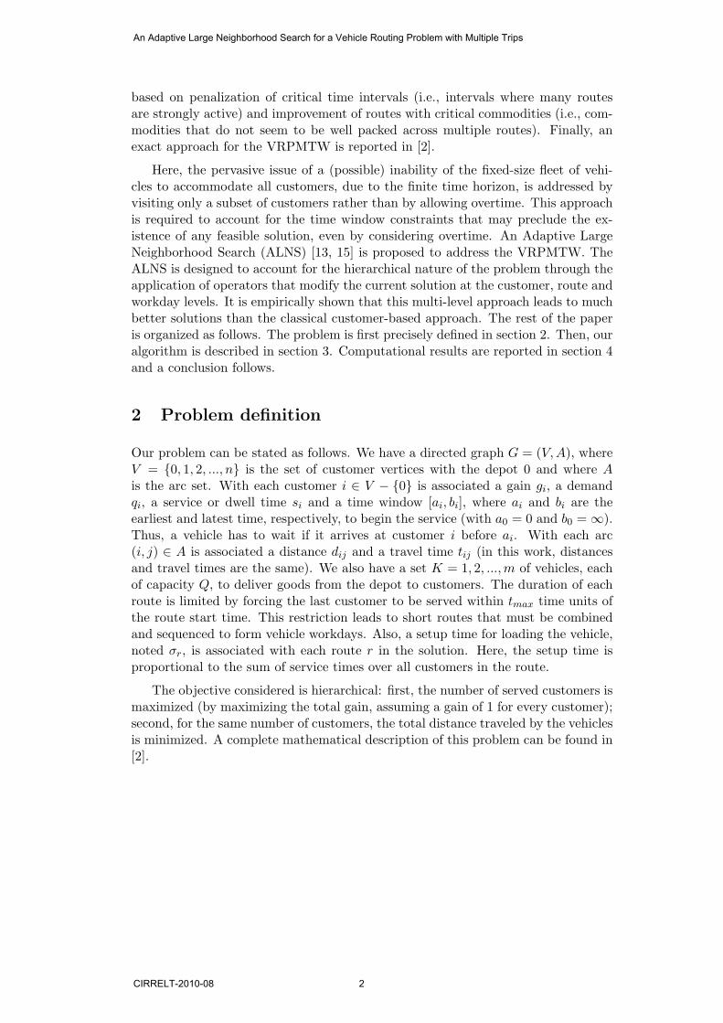
2 Problem definition

Our problem can be stated as follows. We have a directed graph G = (V, A), whereV = {0, 1, 2, ..., n} is the set of customer vertices with the depot 0 and where A

is the arc set. With each customer i ∈ V − {0} is associated a gain gi, a demandqi, a service or dwell time si and a time window [ai, bi], where ai and bi are theearliest and latest time, respectively, to begin the service (with a0 = 0 and b0 =∞).Thus, a vehicle has to wait if it arrives at customer i before ai. With each arc(i, j) ∈ A is associated a distance dij and a travel time tij (in this work, distancesand travel times are the same). We also have a set K = 1, 2, ..., m of vehicles, eachof capacity Q, to deliver goods from the depot to customers. The duration of eachroute is limited by forcing the last customer to be served within tmax time units ofthe route start time. This restriction leads to short routes that must be combinedand sequenced to form vehicle workdays. Also, a setup time for loading the vehicle,noted σr, is associated with each route r in the solution. Here, the setup time isproportional to the sum of service times over all customers in the route.

The objective considered is hierarchical: first, the number of served customers ismaximized (by maximizing the total gain, assuming a gain of 1 for every customer);second, for the same number of customers, the total distance traveled by the vehiclesis minimized. A complete mathematical description of this problem can be found in[2].


CIRRELT-2010-08 2

3 Problem-solving methodology

ALNS extends the large neighborhood search framework of Shaw [17], a problem-solving approach which can also be related to the ruin-and-recreate principle [16].The basic idea is to search for a better solution at each iteration by destroyinga part of the current solution and by reconstructing it in a different way. Whensolving VRPs, a new solution is typically obtained by first removing a number ofcustomers and then by reinserting these customers into the solution. In general, anumber of destruction and reconstruction operators are available and a destruction-reconstruction pair is randomly chosen at each iteration. In the adaptive extension, aweight is associated with each operator and the selection probability of an operator isrelated to its weight, which is adjusted during the search based on its past successes.

The problem structure, where a vehicle workday is made of a sequence of tripsand where each trip is made of a sequence of customers, is exploited by applyingdestruction operators at the workday, route and customer levels, in this order. Thisapproach is described in pseudo-code in Algorithm 1. The idea is to go from gross(high-level) to fine (low-level) refinements. In this algorithm, an initial feasiblesolution s is first constructed. Then, a destruction and a reconstruction operator areprobabilistically chosen based on their current weights. The destruction operatorsare first selected at the workday level, then at the route level and finally at thecustomer level, where each level is explored for a number of consecutive iterations.At each iteration, a new solution is obtained by applying the destruction operatorfollowed by the reconstruction operator on the current solution s. The new solutions′ is then submitted to an acceptance rule. If accepted, the new solution becomesthe current solution, otherwise the current solution does not change. After exploringa given level, the weights associated with the applied operators are adjusted. Thisis repeated until a termination criterion is met and the best solution found s∗ isreturned. In the following, each component of this algorithmic framework will beexplained in detail.

3.1 Construction of the initial solution

An insertion heuristic, where all routes and workdays grow in parallel, is used toobtain an initial solution, see Algorithm 2. Based on a given ordering, each customeris considered in turn and inserted at its best feasible insertion place over every routein every workday, including a new (empty) workday if one is still available. In thiswork, the best insertion place corresponds to the smallest detour in distance, wherethe detour is dji + dil − djl for the insertion of customer i between j and l. If thereis no feasible insertion place for customer i, then each route is considered in turnand split into two subroutes, with an additional copy of the depot between the twosubroutes. This is illustrated in Figure 1, where the square stands for the depot andthe black circle for the customer to be inserted. Once the original route is split, theinsertion of the customer can take place in any of the two new routes. Each route issplit in every possible way (i.e., at every customer location along the route) to findthe best insertion place. If there is still no feasible insertion place, then customer i


CIRRELT-2010-08 3

Algorithm 1 ALNS

1. construct a feasible solution s;2. s∗ ← s;3. initialize weights;4. while the stopping criterion is not met do

4.1 for L = workday, route, customer do

4.1.1 for I iterations do

a. probabilistically select a destruction operator at level L

and a reconstruction operator based on their current weights;b. apply the destruction and reconstruction operators to s

to obtain s′;c. if s′ satisfies the acceptance criterion then

- s← s′;- if s′ is better than s∗ then s∗ ← s′;

4.1.2 adjust weights;5. return s∗.

split

Figure 1: Split

is put in a list of (temporarily) unserved customers. The split procedure proved tobe particularly useful when the infeasibility is due to the tmax constraint.

During this insertion procedure, the vehicle schedule based on the latest feasibledeparture times from the depot is considered to reduce as much as possible routedurations. Let us assume that route r is the last route in a vehicle workday. Thisroute is described by the sequence (0r

d = ir0, ir1, i

r2, ..., i

rnr

, irnr+1 = 0re), where 0r

d and0r

e stand for the departure from and return to the depot, respectively, and nr is thenumber of customers in the route.

To determine the latest schedule of that route, denoted by the latest feasibletime to begin service tirj at each customer irj , j = 1, ..., nr, a backward sweep of theroute is first applied from irnr+1 = 0r

e to ir0 = 0rd as follows:

tirnr+1← birnr+1

,


CIRRELT-2010-08 4

Algorithm 2 Construction heuristic

1. L← {1, 2, ..., n};2. while (L 6= ∅) do

2.1 randomly select customer i ∈ L;2.2 insert customer i at its best feasible insertion place in the solution;2.3 if there is no feasible insertion place in the solution then

2.3.1 for each route k in the solution apply split(i, k);2.4 L← L− {i}.

tirj ← min{tirj+1− tirj irj+1

− sirj, birj}, j = irnr

, ..., ir0.

Once the latest departure time from the depot tir0 is obtained, a forward sweep isapplied from ir0 = 0r

d to irnr+1 = 0re to reset the tirj values and get the latest feasible

schedule:

tirj ← max{tirj−1+ tirj−1irj

+ sirj−1, airj}, j = ir1, ..., i

rnr+1.

The total route duration is tirnr+1− tir0 , which is also the minimum duration,

because the waiting time is minimized by serving the route at the latest feasibletime. The whole procedure is then applied to the second-to-last route r − 1 bysetting

tir−1nr−1+1

← tir0 − σr.

This is repeated until the first route is done.

3.2 Destruction operators

Different destruction operators are defined at the customer, route and workday level.They are described in the following.

3.2.1 Customer level

These operators remove a number n1 of individual customers from the current so-lution.

Random customer removal. This is a very simple approach where the customers arechosen at random.

Related customer removal. This operator is inspired from the one described by Shawin [17]. The main difference is that the proximity measure between two customers isbased on both spatial and temporal characteristics. This operator can be describedas follows (see Algorithm 3).

Starting with a randomly chosen request, which starts the whole procedure, theremoval of the next request is (probabilistically) biased toward those that are close


CIRRELT-2010-08 5

Algorithm 3 Related customer removal

1. randomly select a customer j and remove it from the solution;2. L← {j};3. while | L |< n1 do

3.1 i← randomly select a customer in L;3.2 for each customer j in the solution do

3.2.1 zij ← α · |ti − tj |+ β · dij ;3.3 sort the zij ’s in non decreasing order and put them in list B;3.4 choose a random number x between 0 and 1;3.5 pos← ⌈| B | · xd⌉;3.6 select customer j associated with the zij value at position pos in B

and remove it from the solution;3.7 L← L ∪ {j};

4. return L

to one of the previously removed requests. The proximity between two customersis based on a metric that accounts for both the geographical distance and the ab-solute difference between the time of beginning of service at both customer locations,weighted by parameters α and β, respectively. Parameter d in step 3.5 controls theintensity of the bias. Namely, a high value for parameter d strongly favors the re-moval of requests that are close to previously removed requests (and conversely).Based on preliminary experiments, this parameter was set to 6.

3.2.2 Route level

These operators remove a number n2 of individual routes from the current solution.

Random route removal. This is a very simple approach where the routes are chosenat random.

Related route removal. This is an adaptation of the corresponding customer-basedoperator which is applied at the route level. Accordingly, the algorithmic frameworkis very similar to the one found in Algorithm 3. First, a route is randomly chosen.Then, the removal of the next route is (probabilistically) biased toward those thatare close to one of the previously removed routes.

Two different proximity measures between route rj and some previously removedroute ri have been considered, where it is assumed that a route is defined by its setof customers.

1. GC : zij ← d(grigrj

), where griamd grj

are the gravity centers of routes ri and

rj , respectively.

2. MinD : zij ← mink∈ri,l∈rjdkl.

In the first case, the proximity is measured by the distance between the gravitycenters of routes ri and rj , where the latter is defined as the average location over


CIRRELT-2010-08 6

Algorithm 4 Related route removal

1. randomly select a route rj and remove it from the solution;2. L← {rj};3. while | L |< n2 do

3.1 ri ← randomly select a route in L;3.2 for each route rj in the solution do

3.2.1 zij ← compute the proximity measure between ri and rj ;3.3 sort the zij ’s in non decreasing order and put them in list B;3.4 choose a random number x between 0 and 1;3.5 pos← ⌈| B | · xd⌉;3.6 select route rj associated with the zij value at position pos in B

and remove it from the solution;3.7 L← L ∪ {rj};

4. return L.

all customer locations in the route. In the second case, the proximity is measuredby the smallest distance between any pair of customers taken from routes ri and rj .

3.2.3 Workday level

A single operator is defined at the workday level. It simply removes n3 randomlychosen workdays from the solution.

3.3 Insertion operators

After the application of a destruction operator, the customers that are not partof the solution, either because they have just been removed or because there wasno feasible insertion place for them, are considered for reinsertion. Two differentinsertion heuristics have been defined for this purpose.

3.3.1 Least-cost heuristic

This is the insertion heuristic used for constructing an initial solution (see Algorithm2), except that it is applied only to customers that are not part of the solution.Accordingly, the selection of the next customer is random and its insertion takesplace at the feasible location with minimum detour.

3.3.2 Regret-based heuristic

A second insertion heuristic has been devised to alleviate the myopic behavior ofthe least-cost heuristic. This is done by defining a reinsertion order based on aregret measure. For a given customer, the 2-regret heuristic computes the minimumfeasible detour in each workday. Then, it considers the difference between the detourin the second best and best workday. If this difference is large, the corresponding


CIRRELT-2010-08 7

customer gets high priority for reinsertion because a large cost is incurred if its bestworkday becomes infeasible (due to the insertion of other customers). A generalizedvariant considers the minimum detour in each workday and sums up the differences,over all workdays, between the minimum detour in the workday and the overallminimum detour.

More formally, let us assume that the minimum detour when customer i is in-serted in workday k is detourik and that the overall minimum detour is obtainedwhen customer i is inserted in workday k∗. Then, the generalized regret measure ofcustomer i is:

gen regreti =∑

k=1,...,m

(detourik − detourik∗) .

At each iteration, the customer with the maximum regret measure is selectedfor reinsertion at the feasible insertion place with minimum detour.

3.4 Acceptance criterion

The criterion for accepting or rejecting a new solution is the one used in simulatedannealing [9]. That is, the new solution s′ is accepted over the current solution s ifs′ is better than s. Otherwise, it is accepted with probability

e−f(s′)−f(s)

T

where T is the temperature parameter and f is the objective function. Startingfrom some initial value, the temperature is lowered from one iteration to the nextby setting T ← c · T . Clearly, the probability of accepting a non-improving solutiondiminishes with the value of T , as the algorithm unfolds. This behavior allowsthe algorithm to progressively settle in a (hopefully) good local optimum. In ourexperiments, the starting temperature was set to 1.05 · f(s0), where s0 is the initialsolution, and c to 0.99975, as suggested in [15].

3.5 Adaptive mechanism

The ALNS applies a removal and an insertion operator at each iteration on thecurrent solution. The adaptive mechanism is aimed at choosing the removal andinsertion operators in a way that accounts for their previous outcomes. A weightis associated with each operator for this purpose. Let us assume that we have h

insertion operators, each with a weight wj , j = 1, ..., h. The insertion operator i isthen selected with probability

wi∑h

j=1 wj

, i = 1, ..., h.

That is, the probability of selecting a given operator increases with its weight. Start-ing with a unit weight for each insertion operator, the weights are updated after a


CIRRELT-2010-08 8

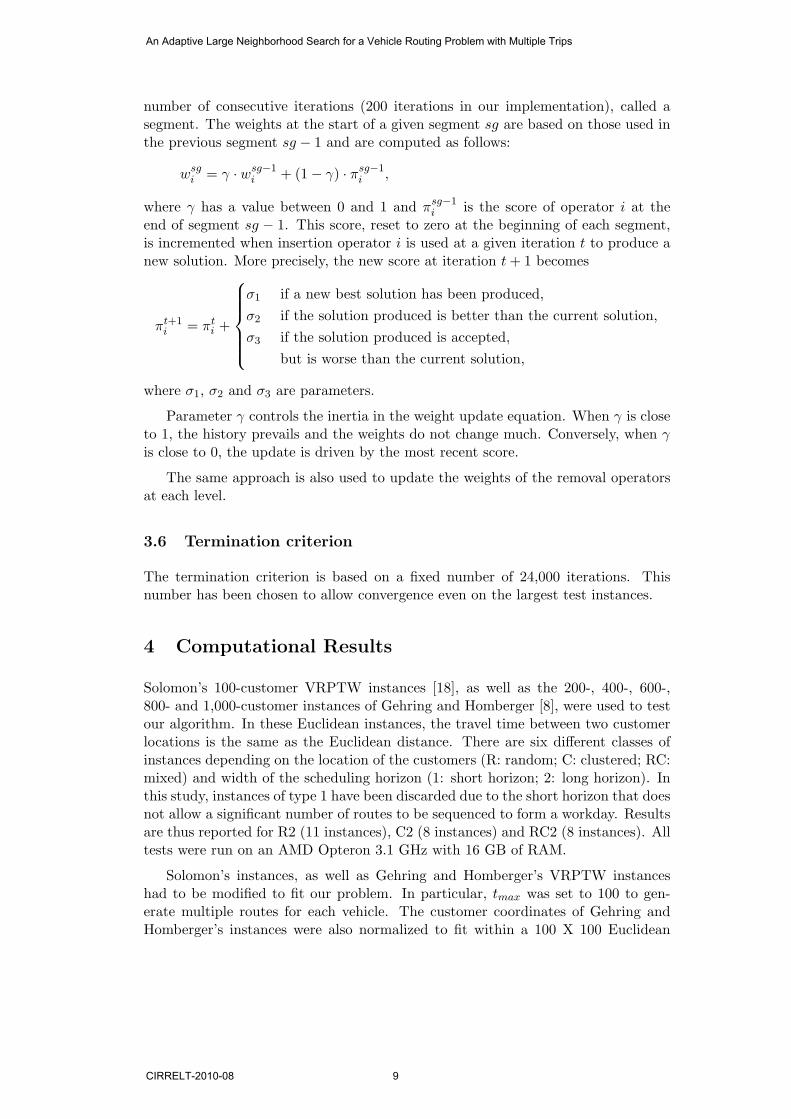
number of consecutive iterations (200 iterations in our implementation), called asegment. The weights at the start of a given segment sg are based on those used inthe previous segment sg − 1 and are computed as follows:

wsgi = γ · wsg−1

i + (1− γ) · πsg−1i ,

where γ has a value between 0 and 1 and πsg−1i is the score of operator i at the

end of segment sg − 1. This score, reset to zero at the beginning of each segment,is incremented when insertion operator i is used at a given iteration t to produce anew solution. More precisely, the new score at iteration t + 1 becomes

πt+1i = πt

i +

σ1 if a new best solution has been produced,

σ2 if the solution produced is better than the current solution,

σ3 if the solution produced is accepted,

but is worse than the current solution,

where σ1, σ2 and σ3 are parameters.

Parameter γ controls the inertia in the weight update equation. When γ is closeto 1, the history prevails and the weights do not change much. Conversely, when γ

is close to 0, the update is driven by the most recent score.

The same approach is also used to update the weights of the removal operatorsat each level.

3.6 Termination criterion

The termination criterion is based on a fixed number of 24,000 iterations. Thisnumber has been chosen to allow convergence even on the largest test instances.

4 Computational Results

Solomon’s 100-customer VRPTW instances [18], as well as the 200-, 400-, 600-,800- and 1,000-customer instances of Gehring and Homberger [8], were used to testour algorithm. In these Euclidean instances, the travel time between two customerlocations is the same as the Euclidean distance. There are six different classes ofinstances depending on the location of the customers (R: random; C: clustered; RC:mixed) and width of the scheduling horizon (1: short horizon; 2: long horizon). Inthis study, instances of type 1 have been discarded due to the short horizon that doesnot allow a significant number of routes to be sequenced to form a workday. Resultsare thus reported for R2 (11 instances), C2 (8 instances) and RC2 (8 instances). Alltests were run on an AMD Opteron 3.1 GHz with 16 GB of RAM.

Solomon’s instances, as well as Gehring and Homberger’s VRPTW instanceshad to be modified to fit our problem. In particular, tmax was set to 100 to gen-erate multiple routes for each vehicle. The customer coordinates of Gehring andHomberger’s instances were also normalized to fit within a 100 X 100 Euclidean


CIRRELT-2010-08 9

100 iterations 200 iterations 400 iterations% % CPU % CPU % CPU

dstr. size unsv. dist. (s) unsv. dist. (s) unsv. dist. (s)

100 28.1 1938.0 42.8 27.8 1923.5 42.4 28.1 1924.9 44.705-35 400 28.0 10940.6 671.6 28.1 10938.0 678.5 28.3 10938.2 671.6

800 30.2 22713.3 2822.9 30.6 22698.9 2898.5 30.3 22830.2 2867.9

100 31.4 1950.9 44.6 32.2 1949.2 44.8 31.5 1960.7 46.835-65 400 29.9 11157.0 745.0 30.0 11185.9 740.3 29.8 11258.1 755.9

800 30.9 22915.8 2966.8 30.9 22976.3 2990.6 31.0 22850.0 2938.1

100 34.0 1966.7 48.5 33.7 1963.7 45.7 35.6 1989.3 52.365-95 400 30.3 11277.1 823.6 30.0 11199.6 807.9 30.1 11230.7 806.7

800 30.5 22896.3 3228.2 30.4 22774.4 3285.2 30.4 22677.3 3224.2

Table 1: Impact of % of destruction and number of iterations at each level

square, as in Solomon’s instances. Furthermore, the service or dwell time at eachcustomer was set to 10 in all instances. The number of vehicles was set to 3 forthe 100-customer instances, and this number was increased to 6, 12, 18, 24 and 30for the 200-, 400-, 600-, 800- and 1,000-customer instances, respectively, to obtaininstances with approximately the same degree of difficulty.

In the following, some parameter sensitivity results are presented. Then, thefinal results on the whole test set are reported. A comparison with known optimalsolutions on small instances with no more than 40 customers are also reported atthe end.

4.1 Parameter sensitivity

We have studied the impact of the number of consecutive iterations at each leveland percentage of destruction (% dstr.) on the algorithmic performance. To thisend, we have used a test set made of the RC2 instances with 100, 400 and 800customers. The results are shown in Table 1. We have considered 100, 200 and 400consecutive iterations at each level (i.e., 300, 600 and 1200 iterations for the wholeworkday-route-customer level sequence). Three different intervals for the percentageof destruction of the current solution were also tested, namely [5%, 35%], [35%, 65%]and [65%, 95%]. When a removal operator is chosen, a percentage value is uniformlyrandomly selected in the corresponding interval and applied at the appropriate level.For each possible combination of the two parameters and for each problem size, Table1 shows the average percentage of unserved customers (% unsv.), total distance(dist.) and computation time in seconds (CPU ).

Not surprisingly, the computation time increases with the percentage of destruc-tion because it is more costly to reinsert a larger number of customers into thecurrent solution. Furthermore, solution quality tends to degrade. Based on theresults shown in Table 1, the best combination is a percentage of destruction in theinterval [5%, 35%] and 200 consecutive iterations at each level (i.e., 600 iterationsfor the whole workday-route-customer sequence and 40 such sequences over 24,000iterations). This setting has been used in the following sections.


CIRRELT-2010-08 10

4.2 Results

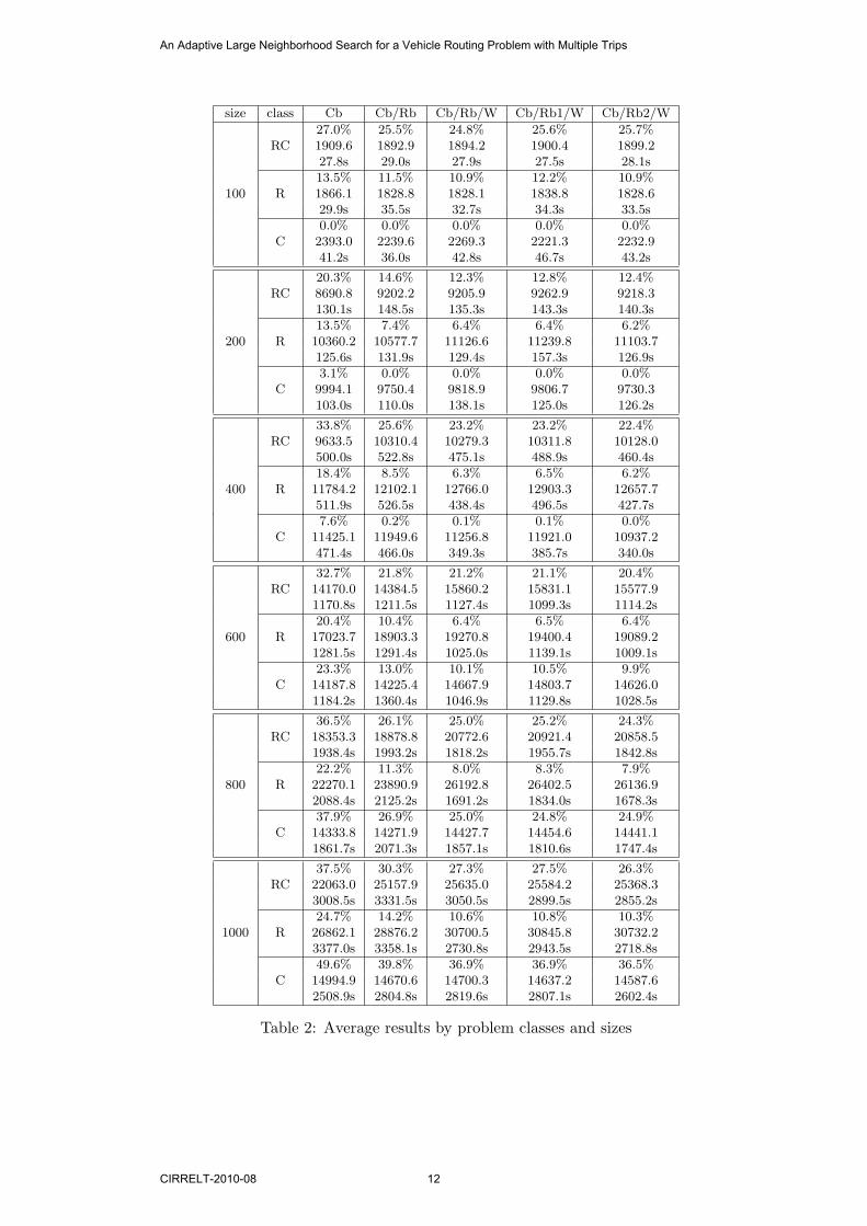
Based on the best parameter setting identified in section 4.1, different variants ofour ALNS have been applied to the whole set of test instances. These results arereported in Table 2. As indicated in this table, five different variants have beenconsidered: Cb only uses the customer-based removal operators, Cb/Rb uses boththe customer- and route-based removal operators while Cb/Rb/W uses all removaloperators. Two variants of Cb/Rb/W have also been tested: Cb/Rb1/W, wherethe related route removal operator using the MinD proximity measure is discarded(thus, only the random route removal and the related route removal using the GCmeasure are considered) and Cb/Rb2/W, where the related route removal using theGC measure is discarded (thus, only the random route removal and the relatedroute removal using the MinD measure are considered). In each entry, we showthe percentage of unserved customers (%), the total distance and the computationtime in seconds (s), in this order. These results are averaged over all sizes for eachproblem class in Table 3.

The first observation is that the exploitation of a multi-level scheme is verybeneficial when compared to the classical customer-based approach. By introducinga route level, the percentage of unserved customers is reduced by 7.81%, 8.22% and6.92% on problem classes RC, R and C, respectively. An additional improvement,although less important, is also obtained by introducing the workday level.

The differences observed between Cb/Rb1/W and Cb/Rb2/W also indicate thatthe related route removal operator using the MinD proximity measure is superiorto the one using the gravity center-based measure. Also, by comparing Cb/Rb2/Wand Cb/Rb/W, a single related route removal operator based on the MinD measureprovides better results than the use of the two operators concurrently.

4.3 Comparison with optimal solutions

The best ALNS variant Cb/Rb2/W has been applied to small instances for whichthe optimum is known and reported in [2]. These instances have been created byconsidering only subsets of 25 and 40 customers in Solomon’s original instances [18].The reported optima have been obtained with tmax = 75 and a fleet of 2 vehicles.Table 4 reports average results obtained over all instances of given class and size.On the 25-customer instances, ALNS is quasi-optimal. All customers are served andthe gap in total distance does not exceed 1%. On the 40-customer instances of typeRC and C, ALNS is also close to the optimum. On the three instances of type R, adifference of 2.5% is observed with regard to the percentage of unserved customersand a gap of 16% with regard to the total distance. But, these average gaps arelargely due to only one particular instance, for which 3 customers are left unservedby ALNS (no unserved customer in the optimal solution) and a gap close to 30% isobserved in total distance.


CIRRELT-2010-08 11

size class Cb Cb/Rb Cb/Rb/W Cb/Rb1/W Cb/Rb2/W

27.0% 25.5% 24.8% 25.6% 25.7%RC 1909.6 1892.9 1894.2 1900.4 1899.2

27.8s 29.0s 27.9s 27.5s 28.1s13.5% 11.5% 10.9% 12.2% 10.9%

100 R 1866.1 1828.8 1828.1 1838.8 1828.629.9s 35.5s 32.7s 34.3s 33.5s0.0% 0.0% 0.0% 0.0% 0.0%

C 2393.0 2239.6 2269.3 2221.3 2232.941.2s 36.0s 42.8s 46.7s 43.2s

20.3% 14.6% 12.3% 12.8% 12.4%RC 8690.8 9202.2 9205.9 9262.9 9218.3

130.1s 148.5s 135.3s 143.3s 140.3s13.5% 7.4% 6.4% 6.4% 6.2%

200 R 10360.2 10577.7 11126.6 11239.8 11103.7125.6s 131.9s 129.4s 157.3s 126.9s3.1% 0.0% 0.0% 0.0% 0.0%

C 9994.1 9750.4 9818.9 9806.7 9730.3103.0s 110.0s 138.1s 125.0s 126.2s

33.8% 25.6% 23.2% 23.2% 22.4%RC 9633.5 10310.4 10279.3 10311.8 10128.0

500.0s 522.8s 475.1s 488.9s 460.4s18.4% 8.5% 6.3% 6.5% 6.2%

400 R 11784.2 12102.1 12766.0 12903.3 12657.7511.9s 526.5s 438.4s 496.5s 427.7s7.6% 0.2% 0.1% 0.1% 0.0%

C 11425.1 11949.6 11256.8 11921.0 10937.2471.4s 466.0s 349.3s 385.7s 340.0s

32.7% 21.8% 21.2% 21.1% 20.4%RC 14170.0 14384.5 15860.2 15831.1 15577.9

1170.8s 1211.5s 1127.4s 1099.3s 1114.2s20.4% 10.4% 6.4% 6.5% 6.4%

600 R 17023.7 18903.3 19270.8 19400.4 19089.21281.5s 1291.4s 1025.0s 1139.1s 1009.1s23.3% 13.0% 10.1% 10.5% 9.9%

C 14187.8 14225.4 14667.9 14803.7 14626.01184.2s 1360.4s 1046.9s 1129.8s 1028.5s

36.5% 26.1% 25.0% 25.2% 24.3%RC 18353.3 18878.8 20772.6 20921.4 20858.5

1938.4s 1993.2s 1818.2s 1955.7s 1842.8s22.2% 11.3% 8.0% 8.3% 7.9%

800 R 22270.1 23890.9 26192.8 26402.5 26136.92088.4s 2125.2s 1691.2s 1834.0s 1678.3s37.9% 26.9% 25.0% 24.8% 24.9%

C 14333.8 14271.9 14427.7 14454.6 14441.11861.7s 2071.3s 1857.1s 1810.6s 1747.4s

37.5% 30.3% 27.3% 27.5% 26.3%RC 22063.0 25157.9 25635.0 25584.2 25368.3

3008.5s 3331.5s 3050.5s 2899.5s 2855.2s24.7% 14.2% 10.6% 10.8% 10.3%

1000 R 26862.1 28876.2 30700.5 30845.8 30732.23377.0s 3358.1s 2730.8s 2943.5s 2718.8s49.6% 39.8% 36.9% 36.9% 36.5%

C 14994.9 14670.6 14700.3 14637.2 14587.62508.9s 2804.8s 2819.6s 2807.1s 2602.4s

Table 2: Average results by problem classes and sizes


CIRRELT-2010-08 12

class Cb Cb/Rb Cb/Rb/W Cb/Rb1/W Cb/Rb2/W31.8% 24.0% 22.3% 22.6% 21.9%

RC 12470.0 13304.5 13941.2 13968.6 13841.71129.3s 1206.1s 1105.7s 1102.4s 1073.5s18.8% 10.6% 8.1% 8.5% 8.0%

R 15027.7 16029.8 16980.8 17115.4 16924.71235.7s 1244.7s 1007.9s 1100.8s 999.0s20.2% 13.3% 12.0% 12.0% 11.9%

C 11221.5 11184.6 11190.2 11307.4 11092.51028.4s 1141.4s 1042.3s 1050.8s 981.3s

Table 3: Average results over all sizes for each problem class

Cb/Rb2/W Optimal# % %

size class instances unsv. distance unsv. distanceRC 5 0.0 844.1 0.0 844.0

25 R 11 0.0 624.1 0.0 620.1C 7 0.0 635.6 0.0 629.1

RC 3 13.9 1386.4 13.3 1377.540 R 3 3.3 1289.0 0.8 1071.6

C 3 0.0 1105.0 0.0 1093.0

Table 4: Comparison with optimal solutions


CIRRELT-2010-08 13

5 Conclusion

This paper has described an adaptation of the ALNS framework based on the hierar-chical structure of the vehicle routing problem with multiple trips. Empirical resultsdemonstrate that it is very beneficial to apply operators at the customer, route andworkday levels, as opposed to the classical approach where only customer-basedoperators are used.

References

[1] Alonso F., Alvarez M.J., Beasley J.E., 2008. “A Tabu Search Algorithm for thePeriodic Vehicle Routing Problem with Multiple Vehicle Trips and AccessibilityRestrictions”, Journal of the Operational Research Society 59, 963-976.

[2] Azi N., Gendreau M., Potvin J.-Y., 2010. “An Exact Algorithm for a VehicleRouting Problem with Time Windows and Multiple Use of Vehicles”, EuropeanJournal of Operational Research 202, 756-763.

[3] Azi N., Gendreau M., Potvin J.-Y., 2007. “An Exact Algorithm for a SingleVehicle Routing Problem with Time Windows and Multiple Routes”, EuropeanJournal of Operational Research 178, 755–766.

[4] Battarra M., Monaci M., Vigo D., 2008. “An adaptive Guidance Approach forthe Heuristic Solution of a Minimum Multiple Trip Vehicle Routing Problem”,Computers & Operation Research, 316–329.

[5] Brandao J.C.S., Mercer A., 1998. “The Multi-Trip Vehicle Routing Problem”,Journal of the Operational Research Society 49, 799–805.

[6] Brandao J.C.S., Mercer A., 1997. “A Tabu Search Algorithm for the Multi-TripVehicle Routing and Scheduling Problem”, European Journal of OperationalResearch 100, 180–191.

[7] Fleischmann B., 1990. “The Vehicle Routing Problem with Multiple Use ofVehicles”, Working Paper, Fachbereich Wirtschaftswissenschaften, UniversitatHamburg, Germany.

[8] Gehring H., Homberger J., 1999.“A Parallel Hybrid Evolutionary Metaheuristicfor the Vehicle Routing Problem with Time Windows”. In: K. Miettinen, M.M.Makela, J. Toivanen (Eds.), Proceedings of EUROGEN99 - Short Course onEvolutionary Algorithms in Engineering and Computer Science, Reports of theDepartment of Mathematical Information Technology, No. A 2/1999, Universityof Jyvaskyla, 57–64.

[9] Kirkpatrick S., Gelatt Jr. C.D., Vecchi M.P., 1990. “Optimization by SimulatedAnnealing”, Science 220, 671–680.


CIRRELT-2010-08 14

[10] Olivera A., Viera O., 2007. “Adaptive Memory Programming for the VehicleRouting Problem with Multiple Trips”, Computers & Operations Research 34,28–47.

[11] Petch R.J., Salhi S., 2003.“A Multi-Phase Constructive Heuristic for the VehicleRouting Problem with Multiple Trips”, Discrete Applied Mathematics 133, 69–92.

[12] Petch R.J., Salhi S., 2007.“A GA Based Heuristic for the Vehicle Routing Prob-lem with Multiple Trips”, Journal of Mathematical Modelling and Algorithms6, 591–613.

[13] Pisinger D., Ropke S., 2007. “A General Heuristic for Vehicle Routing Prob-lems”, Computers & Operations Research 34, 2403–2435.

[14] Rochat Y., Taillard E., 1995. “Probabilistic Diversification and Intensificationin Local Search for Vehicle Routing”, Journal of Heuristics 1, 147–167.

[15] Ropke S., Pisinger D., 2006. “ An Adaptive Large Neighborhood Search Heuris-tic for the Pickup and Delivery Problem with Time Windows”, TransportationScience 40, 455–472.

[16] Schrimpf J., Schneider H., Dueck G., 2000. “Record breaking optimization re-sults using the ruin and recreate principle”, Journal of Computational Physics159, 139–171.

[17] Shaw P., 1998. “Using constraint programming and local search methods tosolve vehicle routing problems”, In: G. Goos, J. Hartmanis and J. van Leeuwen(Eds.), Principles and Practice of Constraint Programming - CP98, LectureNotes in Computer Science 1520, 417–431.

[18] Solomon M.M., 1987.“Algorithms for the Vehicle Routing and Scheduling Prob-lem with Time Window Constraints”, Operations Research 35, 254–265.

[19] Taillard E. D., Laporte G., Gendreau M., 1996.“Vehicle Routeing with MultipleUse of Vehicles”, Journal of the Operational Research Society 47, 1065–1070.

[20] Toth P., Vigo D., 2002. The Vehicle Routing Problem. SIAM Monographs onDiscrete Mathematics and Applications, Philadelphia, PA.


CIRRELT-2010-08 15

Documents

An Adaptive Large Neighborhood Search for a … · An Adaptive Large Neighborhood Search for a Vehicle Routing Problem with Multiple Trips Nabila Azi Michel Gendreau Jean-Yves Potvin