An Active Position Sensing Tag for SportsVisualization in American Football

Darmindra D. Arumugam1, Michael Sibley2, Joshua D. Griffin3, Daniel D. Stancil4, David S. Ricketts51Jet Propulsion Lab., California Institute of Technology, Pasadena, CA, Email: Darmindra.D.Arumugam@jpl.nasa.gov

2Tait Towers, Lititz, PA, Email: mike.sibley@gmail.com3Disney Research, Pittsburgh, PA, Email: joshdgriffin@disneyresearch.com

4,5North Carolina State University, Raleigh, NC, Email: 4ddstancil@ncsu.edu 5david.ricketts@ncsu.edu

Abstract—Remote experience and visualization in sportingevents can be significantly improved by providing accuratetracking information of the players and objects in the event.Sporting events such as American football or rugby have proveddifficult for camera- and radio-based tracking due to blockageof the line-of-sight, or proximity of the ball to groups of players.Magnetoquasistatic fields have been shown to enable accurateposition and orientation sensing in these environments [1]–[3]. Inthis work, we introduce a magnetoquasistatic tag developed fortracking an American football during game-play. We describe itsintegration into an American football and demonstrate its use ingame-play during a collegiate American football practice.

I. INTRODUCTION

The use of camera-based and wireless localization technol-ogy in sports is growing for application such as athlete training,game analysis, and visualization [4]. However, localization inmany sport environments is challenging because the line-of-sight (LoS) to the person/object to be tracked can be blockedby the bodies of players. This situation is common for balltracking in American football or rugby where the ball can beburied under several player’s bodies or held close to a player’sbody. In such situations, localizing the ball with a camerais difficult and conventional localization systems, such asultra-wideband (UWB), satellite-based, and backscatter radiofrequency identification (RFID), will suffer reduced accuracy.

In an effort to meet these challenges, a tracking systembased on magnetoquasistatic fields has been developed, andstudied in detail, to determine both the position and orientationof a sensor when the LoS is blocked and the sensor is closeto lossy dielectrics (e.g., player’s bodies) [1]–[3], [5]. Thetracking system measures the magnitude of the magnetic fieldgenerated by a small magnetic dipole antenna at multiple spa-tial location and then inverts the field equations to determinethe sensor’s position and orientation.

In this paper, we characterize the active RF tag foruse in magnetoquasistatic position sensing of an Americanfootball during actual game-play. The tag is integrated intoan American football and its operation presented during anactual play. The technique, algorithm, and accuracy have beenpreviously reported for the one-dimensional (1D) case in [1],two-dimensional case in [5], three-dimensional case in [2],and for a goal-line play in [3]. In [1], we demonstrated a 1Ddistance estimation error 11.74 cm for distances between 1.3

D.D. Arumugam and M. Sibley performed this work at Disney Research.

1

0

1

0

Receive Loops

1

2

3 4 5 6

7

8

Magnetic FieldLines Filter

ADC

Amp.

LoopAntenna

Transmitter

Battery

Fig. 1. Magnetoquasistatic positioning system setup. The football is equippedwith an integrated transmitter that emits quasistatic magnetic fields. Eightreceivers, positioned around region of the field extending from the back ofthe end-zone to the ten yard line, were used to track the ball from the backof the end-zone to approximately the 15 yard line.

and 34.2 m, whereas in [2], we showed a mean 3D positionerror of 0.77 m, a mean inclination orientation error of 9.67◦,and a mean azimuthal orientation error of 2.84◦.

A brief overview of the system is provided in Section II andthe design of the active RF tag is discussed in Section III. Theball’s integration into a football is presented in Section IV;the integrated tag’s performance under various conditions isdiscussed in Section V; and a preliminary study of the specificabsorption rate (SAR) induced in an adult male is reported inSection VI. Finally, results from the system’s use in a collegiatefootball practice are presented in Section VII.

II. SYSTEM DESIGN

The magnetoquasistatic tracking system is shown in Fig.1. An electrically-small loop, or transmitter, is used to pref-erentially excite magnetoquasistatic fields that are sensed bymultiple receiving antennas whose positions and orientationsare known. By knowing the magnetic moment of the trans-mitter, the position and orientation of the transmit loop canbe determined using the governing field equations and a least-squares solver [1], [2].

In the American football application, there are severalrequirements for the tracking system. The first is that thereceive antennas must be placed out of the active playingfield, resulting in a maximum transmitter-to-receiver distanceof approximately 50 m. The second is that the transmittermust be seamlessly integrated into the football so as not todisturb its performance, in particular the transmitter’s weight

Loopantenna

Oscillator

Charging circuitry

Rechargeablebattery

SwitchTransmit modeCharging mode

Fig. 2. Block diagram of the magnetoquasistatic tag and loop antenna.

should be less than the variation of an average football, whichis approximately 28 g [6]. Finally, the transmitter must bedurable and accurate to provide tracking during play, whenthe football may be under physical stress, e.g., the weight of abody as well as when in close proximity to the player’s bodies.

Our approach is shown in Fig. 1, where the loop is coiledaround the air-bladder of the football, and the circuit andbattery are located between the air-bladder and the outerleather enclosure. Here, we define the football coil antenna,associated circuitry and battery as the RF tag as shown inFig. 2. The choice of tag operating frequency is determinedby two competing requirements: 1) the quasistatic region (!λ, where λ is the wavelength of the magnetic field) mustbe large and is achieved using a low frequency (which alsoreduces the effects of small, interfering objects and players);and 2) a strong coupling between the transmitter and receiversis required for a good signal-to-noise ratio (SNR), which canbe achieved at a higher frequency. We choose a frequency ofapproximately 400 kHz to balance these two requirements andstay below the AM broadcast band [1].

III. FOOTBALL TAG DESIGN

The transmitter integrated into the American football con-sists of an oscillator circuit connected to a multi-turn loopantenna. The oscillator circuit is powered by a rechargeablebattery that is inductively charged using the same antennaas shown in Fig. 2. Since the integrated transmitter must notdisturb the dynamics of the ball during game-play, care must begiven to the placement and weight of the integrated transmitter.The weight of the battery, circuitry, and antenna were chosento be less than the weight tolerance of an American football(28 g) used in the National Football League [6].

Fig. 3. Impedance of the coil used as the transmitting loop antenna is shownin (a). The inset of (a) shows the multi-turn coil and capacitor for the antenna,where r0=8.25 cm, and N = 45. The capacitor, which is labeled C5 in Fig.5, was chosen to resonate the inductance of the loop at 376 kHz. The returnloss is shown in (b).

0 20 40 60 80 1000

5

10

15

20Mass vs. Number of Turns

Ma

ss (

g)

Number of Turns

12 AWG16 AWG20 AWG24 AWG28 AWG30 AWG32 AWG

Fig. 4. Mass of the coil antenna as a function of the number of loop turns.

A. Antenna Design

To preferentially excite a magnetic field, a coiled loopantenna was used with the transmitter. The antenna was coiledaround the air-bladder and underneath the outer leather ofthe football as shown in the inset of Fig. 1. It consistedof a multi-turn loop as depicted in the inset of Fig. 3. Thecoil antenna had a radius, r0, of 8.25 cm to accommodatethe radius of the American football. We used 45 turns ofclosely wound, 30 AWG (American Wire Gauge) wire to limitthe weight to 10.33 g, and resonated the loop inductancewith a series capacitor to obtain a resonant frequency ofapproximately 376 kHz. The real and imaginary impedance ofthe resonant loop antenna, measured using a vector networkanalyzer (VNA), is shown in Fig. 3a. The measured returnloss, shown in 3b, verifies the resonant frequency of 376 kHz.

Figure 4 shows the calculated mass of the coil antenna as afunction of number of turns. The dashed lines indicate valuesfor the 45-turn coil using 30 AWG wire, as used in the design.The magnetic moment of the coil antenna is dependent on thenumber of turns and current flowing through those turns. As weincrease the number of turns, we must increase the wire gaugeto maintain our target weight of approximately 10g. A higherwire gauge leads to a larger resistance, which reduced currentwhen a class-E source is used. Thus, there is a diminishingreturn on increasing the number of turns and we found 45turns to be a good design point. A complete optimization ofturns and gauge is the subject of future work.

B. Oscillator Circuit

The principle requirements of the football oscillator arethat it be lightweight, have high efficiency, and have relativelyhigh output power. Through experimentation, we found thatan output power of approximately 0.5 W was required toachieve adequate SNR for distances up to the width of theAmerican football field. We satisfied these requirements usinga 45-turn coil loop antenna driven by a class-E oscillator circuitwith power supplied through a 3.3V rechargeable battery, asshown in Fig. 5. A high-efficiency class-E design procedure

Loopantenna

Fig. 5. The class-E oscillator circuit design used for the transmitter.

0 50 100 150 200-10

-5

0

5

10Load Voltage vs. Time

Time (us)

Vo

ltag

e (

V)

On

Off

Fig. 6. Transient load voltage measured at the terminals of the 45-turn coilantenna connected to the output of the class-E oscillator.

[7] was used to obtain an oscillation frequency and efficiencyof 376 kHz and 93%, respectively, with an output power of0.56 W and a current of 159 mArms flowing through the coilantenna [5].

To study the transient characteristics, the antenna wasconnected to the output terminal of the oscillator and thetransient characteristic of the load voltage across the antennaterminals was measured using a high-impedance digital oscil-loscope, shown in Fig. 6. The oscillator load voltage requiredapproximately 15-20 µs and 90-100 µs to achieve the 25%and 10% margin of error in voltage (stable to within 75% and90%, respectively), respectively.

To accommodate reuse, the oscillator circuit is poweredwith a rechargeable battery and charging is accomplished byadding circuitry that receives energy through the transmit loopantenna, shown in Fig. 7a. A surface mount switch is used tochange the circuit from transmitting mode to charging modeand charging occurs when the integrated ball is placed in closeproximity to a secondary transmitting loop as shown in Fig. 8.The charging circuitry consists of a full-wave bridge rectifier,a voltage regulator, and a microcontroller to enable lithium-polymer battery charging. The fabricated and populated com-plete circuit with charging and oscillator is shown in Fig.7b. The rechargeable battery used for the football applicationwas a lithium-polymer type (PRT-10718 by Sparkfun), with acapacity of 400 mAh, a maximum current draw of 800 mA,and a weight of 9 g. The populated circuit board weighed atotal of 7.18 g and had a dimension of 39.5 mm × 33.0 mm.The total RF tag weight was 26.51 g, which is below the28 g requirement. This included the antenna, oscillation andcharging circuitry, and rechargeable battery.

To study the drain characteristics, the battery was fullycharged and drained by switching the circuit to the transmit

5 VRegulator

Li-PoCharger

Class EOsc.

Antenna

Charging Circuitry

To Battery ToAntenna

(a) (b)

Battery

Switch

Fig. 7. The transmitting circuit equipped with a charging circuitry to allow forwireless charging of the rechargeable battery is shown in (a). The fabricatedand populated circuit with integrated wireless charging is shown in (b).

Charging circuitry

Rechargeablebattery

Source Amp.

(a) (b) (c)

Amp.

Matchingcircuit

Loop usedfor charging

Fig. 8. The charging system block diagram is shown in (a). A photo ofthe setup is shown in (b), where the output impedance of the amplifier wasmatched to the loop using matching circuit. A photo of the secondary loopwrapped around a box and used for charging is shown in (c). The integratedfootball was placed inside the box during charging.

mode. Figure 9a shows a plot of the voltage as a functionof time in the transmit mode, measured at the terminalsof the battery. The battery capacity and maximum currentdraw allows for uninterrupted use of the football transmitterfor a period of approximately 4 hours and 45 minutes. Byswitching to charging mode, the circuit stops behaving asa transmitter and instead converts any induced currents intoenergy to recharge the battery. A secondary loop connectedto a signal generator through an amplifier was used to supplythe inductive field during charging, as shown in Fig. 8. Thesignal generator’s output power of +10 dBm was used alongwith +30dB of amplification to achieve +40dBm output tothe terminals of the resonant loop (made of 100 turns of 30AWG wire) at approximately 538 kHz. The charging coil waswrapped around a football packaging box with a dimension ofapproximately 17 cm x 17 cm. The integrated ball was placedinside the box to charge it’s battery. Both the charging andtransmitting loops were placed parallel to each other and ata separation of approximately 2 cm. Figure 9b shows a plotof the voltage as a function time in charging mode, measuredat the terminals of the battery. The inductive charging takesapproximately 13 hours and 40 minutes to fully charge therechargeable battery in the present configuration. This ratherlengthy time is due to the high-loss of the charging loop and anon-optimized impedance match between the charging sourceand load. It was suitable, however, for overnight charging, asneeded for testing.

00:00 00:30 01:00 01:30 02:00 02:30 03:00 03:30 04:00 04:30 05:002

3

4

5

Volta

ge (

V)

Time (HH:MM)

Battery Voltage vs.Time (Drain)

00:00 02:00 04:00 06:00 08:00 10:00 12:00 14:00 16:002

3

4

5

Volta

ge (

V)

Time (HH:MM)

Battery Voltage vs.Time (Charge)

(a)

(b)

Fig. 9. Drain (a) and charge (b) characteristics as a function of time for theintegrated oscillator with charging circuitry.

00:00 01:00 02:00 03:00 04:00381.5

382F

req

(kH

z)

-3

-2

-1

0

05:00

Frequency and Power vs. Time

Time (HH:MM)

Transient effects

Off

Fig. 10. Measured power and frequency as a function of time for theintegrated transmitting circuitry. Initial transient effects are observed withinthe first 15 min., which are likely caused by internal heating.

C. Tag Operation

Figure 10 shows measurements of the relative power andfrequency of the emitted magnetic field as function of time.The magnetic field is measured using a co-polarized receiveantenna (model LFL-1010 from Wellbrook Communications)at a distance of approximately 2 m from the football transmitterand a spectrum analyzer with a resolution bandwidth of300 Hz. Initial transient effects show rapidly changing receivedpower and center frequency within 15-20 minutes of the turn-on time. Therefore, tags were used after an approximately 25-minute warm-up period. The tag shows a total stable operationtime of approximately 4 hours, which safely covers operationover the length of an entire football game. The oscillationfrequency is found to be approximately 381.6 kHz, whichis different from the antenna resonance and circuit design,which was 376 kHz. This is due variability in componentsfrom one board to another, and due to changes in oscillationcharacteristics after integration into an American football.

IV. INTEGRATION INTO AN AMERICAN FOOTBALL

The integration of the magnetoquasistatic tag into thefootball required placement of the transmit loop, circuitry, and

(a) (b) (c)

(d) (e)

(g)(f)

Fig. 11. Integration of the transmitting circuitry, loop antenna, and recharge-able battery into the American football.

battery inside the football so that it could be used unhinderedduring game-play. A commercially-available reproduction ofan NFL football was used for the integration. The footballwas constructed of a leather outer shell, a rubber air blad-der, and a plastic lacing to seal the ball. To integrate themagnetoquasistatic tag, the football was first deflated andcarefully deconstructed. The lacing was untied (Fig. 11a) andthe additional stitching holding the ball opening was cut (Fig.11b). The rubber bladder and the air nozzle were also removedfrom the leather shell (Fig. 11c). The air bladder, now freefrom the leather shell, was re-inflated to match the insidedimension of the shell. The purpose of re-inflation was toallow the emitting loop to be wrapped around the air bladder.The loop was wrapped around the small diameter of the airbladder and the plane of the loop was orthogonal to the longaxis of the ball (Fig. 11d). Cloth-backed adhesive tape wasused to prevent the antenna from shifting on the flexible rubbersurface. Another layer of tape was placed on top of the antennaand the assembly was taped to the rubber bladder at severalintervals to prevent the antenna from shifting while beinginstalled. The bladder and antenna were then inserted underthe leather shell as outlined in the following steps: First, thebladder was deflated and the air nozzle was reinserted throughthe existing hole (Fig. 11e). Next, the remainder of the bladderwas fed through the opening into the ball and partially inflated.The oscillator circuit was attached to the loop and the systemtested. Next, the transmitter circuitry was covered with epoxyto protect it during use, and was then placed along with thebattery inside the ball (Fig. 11f). The circuit was secured withglue to the inside of the leather to prevent shifting while inuse. To allow access to the switch, it was positioned below oneof the existing holes for the football lacing, where it could beaccessed using tweezers or a similar tool. The football lacingwas then replaced (Fig. 11g) and the ball was fully inflated.

V. PERFORMANCE IN FOOTBALLThe integrated football was put through a series of tests

in order to ensure its stability and study its performanceduring game-play. These tests measured signal variations withdifferent air pressures, force loading on the football, dielectric

(a) (b)

(c) (d)

Vector forcemeasurement

platform

Fig. 12. Experiments conducted to determine the performance of theintegrated football: The football air-pressure test is shown in (a); The forcetest is shown in (b); The dielectric (human hand/arm) loading test is shownin (c); The kick (or impact) test is shown in (d).

0 2 4 6 8 10 12 14 16381

382

383

384 Frequency vs. PressureF

requency

(kH

z)

Pressure (psi)

0 2 4 6 8 10 12 14 16-1

-0.5

0 Power vs. Pressure

Pow

er

(dB

)

Pressure (psi)

Specs.

Specs.

(a)

(b)

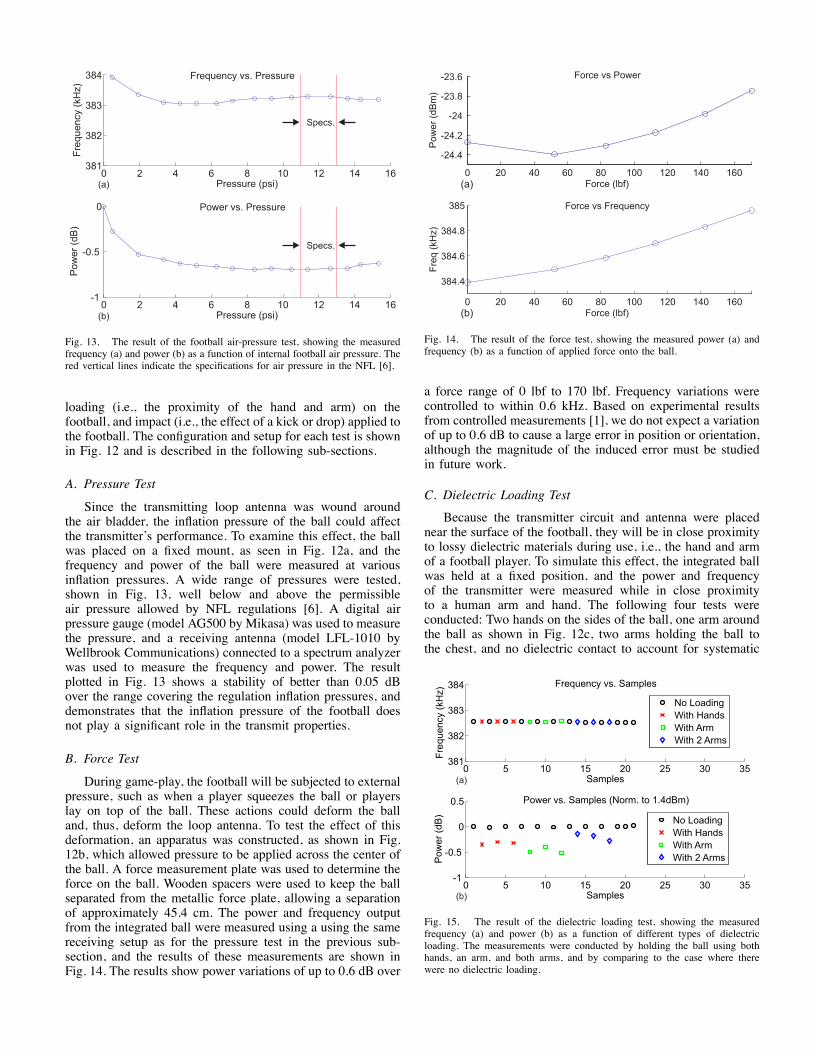
Fig. 13. The result of the football air-pressure test, showing the measuredfrequency (a) and power (b) as a function of internal football air pressure. Thered vertical lines indicate the specifications for air pressure in the NFL [6].

loading (i.e., the proximity of the hand and arm) on thefootball, and impact (i.e., the effect of a kick or drop) applied tothe football. The configuration and setup for each test is shownin Fig. 12 and is described in the following sub-sections.

A. Pressure Test

Since the transmitting loop antenna was wound aroundthe air bladder, the inflation pressure of the ball could affectthe transmitter’s performance. To examine this effect, the ballwas placed on a fixed mount, as seen in Fig. 12a, and thefrequency and power of the ball were measured at variousinflation pressures. A wide range of pressures were tested,shown in Fig. 13, well below and above the permissibleair pressure allowed by NFL regulations [6]. A digital airpressure gauge (model AG500 by Mikasa) was used to measurethe pressure, and a receiving antenna (model LFL-1010 byWellbrook Communications) connected to a spectrum analyzerwas used to measure the frequency and power. The resultplotted in Fig. 13 shows a stability of better than 0.05 dBover the range covering the regulation inflation pressures, anddemonstrates that the inflation pressure of the football doesnot play a significant role in the transmit properties.

B. Force Test

During game-play, the football will be subjected to externalpressure, such as when a player squeezes the ball or playerslay on top of the ball. These actions could deform the balland, thus, deform the loop antenna. To test the effect of thisdeformation, an apparatus was constructed, as shown in Fig.12b, which allowed pressure to be applied across the center ofthe ball. A force measurement plate was used to determine theforce on the ball. Wooden spacers were used to keep the ballseparated from the metallic force plate, allowing a separationof approximately 45.4 cm. The power and frequency outputfrom the integrated ball were measured using a using the samereceiving setup as for the pressure test in the previous sub-section, and the results of these measurements are shown inFig. 14. The results show power variations of up to 0.6 dB over

0 20 40 60 80 100 120 140 160

-24.4

-24.2

-24

-23.8

-23.6 Force vs Power

Force (lbf)

Pow

er

(dB

m)

0 20 40 60 80 100 120 140 160

384.4

384.6

384.8

385 Force vs Frequency

Force (lbf)

Fre

q (

kHz)

(a)

(b)

Fig. 14. The result of the force test, showing the measured power (a) andfrequency (b) as a function of applied force onto the ball.

a force range of 0 lbf to 170 lbf. Frequency variations werecontrolled to within 0.6 kHz. Based on experimental resultsfrom controlled measurements [1], we do not expect a variationof up to 0.6 dB to cause a large error in position or orientation,although the magnitude of the induced error must be studiedin future work.

C. Dielectric Loading Test

Because the transmitter circuit and antenna were placednear the surface of the football, they will be in close proximityto lossy dielectric materials during use, i.e., the hand and armof a football player. To simulate this effect, the integrated ballwas held at a fixed position, and the power and frequencyof the transmitter were measured while in close proximityto a human arm and hand. The following four tests wereconducted: Two hands on the sides of the ball, one arm aroundthe ball as shown in Fig. 12c, two arms holding the ball tothe chest, and no dielectric contact to account for systematic

(a)

(b)

0 5 10 15 20 25 30 35381

382

383

384 Frequency vs. Samples

Fre

quency

(kH

z)

Samples

No Loading

With Hands

With Arm

With 2 Arms

0 5 10 15 20 25 30 35-1

-0.5

0

0.5 Power vs. Samples (Norm. to 1.4dBm)

Pow

er

(dB

)

Samples

No Loading

With Hands

With Arm

With 2 Arms

Fig. 15. The result of the dielectric loading test, showing the measuredfrequency (a) and power (b) as a function of different types of dielectricloading. The measurements were conducted by holding the ball using bothhands, an arm, and both arms, and by comparing to the case where therewere no dielectric loading.

0 0.5 1 1.5 2-10

0

10

Load Voltage vs. Time

Time (s)

Vo

ltag

e (

V)

0 0.1 0.2 0.3 0.4 0.5-10

0

10

Load Voltage vs. Time

Time (s)

Vo

ltag

e (

V)

Contact

Contact

Drop Test

Kick Test

(a)

(b)

Fig. 16. The result of the impact test, showing the measured voltage whenthe football was dropped to the ground (a), and when the football was kicked(b), as a function of time. The region highlighted in red denotes where thefootball is observed to have contact with the ground and the kicker’s foot.

changes in the transmitter’s characteristics. The transmitter’spower and frequency were measured using same setup usedpreviously. Figure 15 shows the result for power and frequencyvariations of the transmitted magnetic field in the experiment.The measured frequency is shown to be almost constant,whereas the measured power varies by as much as 0.5 dB. Weexpect this to induce a small error in position and orientationdetermination, which must be further studied.

D. Impact Test

The football will be subjected to frequent impact in game-play when, for example, the ball is kicked or when it hitsthe ground from a drop. To test the effect of impact on thetransmitted fields, a ball was instrumented with the circuitexternal to the ball to allow access to the circuit for mon-itoring of the generated load voltage at the terminal of theantenna. The monitoring of the load voltage on the externalcircuit allowed us to see the changes in voltage caused byimpact separate from those that would be caused by changesin the ball’s position/orientation if the ball were monitoredwirelessly. The voltage across the antenna was measured withan oscilloscope while the ball was dropped to the ground andwhile it was kicked. The ball was held in place with tapewhen the ball was kicked, as shown in Fig. 12d. The resultsin 16 show transient effects due to the impact caused by thekick and drop. The effects are not noticeable beyond the timewhere contact is visible (measured using a high-speed camerawith 1000 fps). The load voltage is shown to largely returnto its original value. More detailed testing is needed to studyhysteresis effects associated with impact tests.

VI. HUMAN EXPOSURE STUDY

To determine whether or not the instrumented football wassafe for testing with people, a preliminary study was conductedby the IT’IS Foundation to evaluate the instrumented ball’sspecific absorption rate (SAR) induced in a typical adultmale [8]. The study did not consider the football’s impact onimplanted medical devices, and was done through simulation

(b) (c) (d)d

0 dB

-4

-8

-12

-16

-20

Spatial PeakSAR in dB

(a)

Fig. 17. The orientation of the simulated loop antenna with respect to thehomogeneous phantom is shown in (a). The human model and the emittingloop antenna spaced 1 mm from the model’s torso is shown in (b-d). Thisfigure is modified from Fig. 1 and 6 in [8].

using the low-frequency (LF) solver in SEMCAD X v14.6 – amagnetoquasistatic solver implemented with the finite elementmethod (FEM). The instrumented football was modeled as asingle-turn, 163 mm-diameter loop with 8.5 Arms current. Thecurrent of 8.5 Arms was obtained from calculations basedon a 50-turn 34 AWG loop carrying 170 mArms, whichapproximates the football transmitter. The value of 170 mArmsis higher than that found in Section IIIb (159 mArms), andtherefore represents a conservative estimate. Two simulationswere conducted. In the first, the SAR exposure was calculatedwith the outer edge of the loop spaced a small distancefrom a homogeneous phantom – i.e., a rectangular volumewhose homogeneous electromagnetic properties matched thatof human muscle tissue – as shown in Fig. 17a. The separationdistance was set to 0.5 mm, 1 mm, and 2 mm and the 1gpeak spatial SAR (psSAR)1 calculated. Then, to evaluate aworst case scenario, the 1g psSAR results were scaled toreflect a rectangular volume filled with cerebrospinal fluid(CSF) whose conductivity is much higher than muscle tissue.The results from this simulation are given in Table I. In thesecond simulation, the current-carrying loop was simulated inclose proximity to a model of an adult, human male derivedfrom magnetic resonance imaging (MRI) scans. The loop wasspaced a distance of 1 mm from the torso of the human model,as shown in Fig. 17b-d, and the 1g psSAR and whole-bodySAR results are shown in Table II. It can be seen that, forboth simulations, the SAR result are at least one order ofmagnitude below the Federal Communications Commission(FCC) limits2. Therefore, this preliminary study suggests thatthe instrumented ball is safe for testing with people, excludingpersons with implanted medical devices.1The FCC SAR limits for general population/uncontrolled exposure are

based on ANSI/IEEE standard C95.1-2005 [9] and state that the maximumSAR exposure is 0.08 W/kg averaged over the whole-body with the caveat thatthe psSAR cannot exceed 1.6 W/kg averaged over any 1 gram of tissue. Forthe hands, wrists, feet and ankles, the psSAR is limited to 4 W/kg averagedover any 10 grams of tissue.

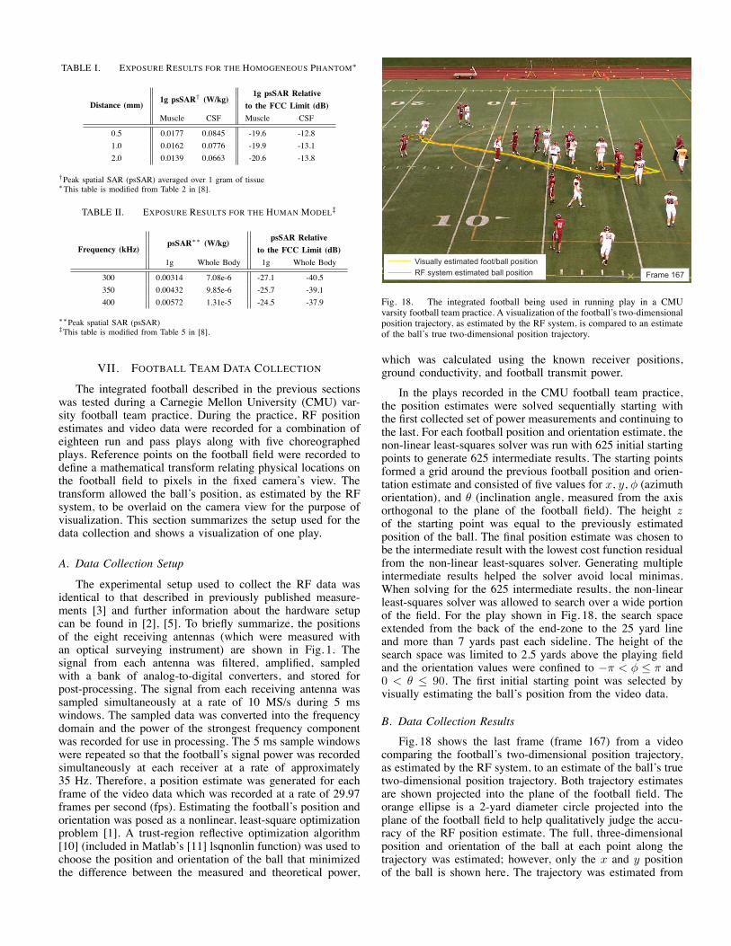
TABLE I. EXPOSURE RESULTS FOR THE HOMOGENEOUS PHANTOM∗

Distance (mm) 1g psSAR† (W/kg)1g psSAR Relative

to the FCC Limit (dB)Muscle CSF Muscle CSF

0.5 0.0177 0.0845 -19.6 -12.81.0 0.0162 0.0776 -19.9 -13.12.0 0.0139 0.0663 -20.6 -13.8

†Peak spatial SAR (psSAR) averaged over 1 gram of tissue∗This table is modified from Table 2 in [8].

TABLE II. EXPOSURE RESULTS FOR THE HUMAN MODEL‡

Frequency (kHz)psSAR∗∗ (W/kg) psSAR Relative

to the FCC Limit (dB)1g Whole Body 1g Whole Body

300 0.00314 7.08e-6 -27.1 -40.5350 0.00432 9.85e-6 -25.7 -39.1400 0.00572 1.31e-5 -24.5 -37.9

∗∗Peak spatial SAR (psSAR)‡This table is modified from Table 5 in [8].

VII. FOOTBALL TEAM DATA COLLECTION

The integrated football described in the previous sectionswas tested during a Carnegie Mellon University (CMU) var-sity football team practice. During the practice, RF positionestimates and video data were recorded for a combination ofeighteen run and pass plays along with five choreographedplays. Reference points on the football field were recorded todefine a mathematical transform relating physical locations onthe football field to pixels in the fixed camera’s view. Thetransform allowed the ball’s position, as estimated by the RFsystem, to be overlaid on the camera view for the purpose ofvisualization. This section summarizes the setup used for thedata collection and shows a visualization of one play.

A. Data Collection Setup

The experimental setup used to collect the RF data wasidentical to that described in previously published measure-ments [3] and further information about the hardware setupcan be found in [2], [5]. To briefly summarize, the positionsof the eight receiving antennas (which were measured withan optical surveying instrument) are shown in Fig. 1. Thesignal from each antenna was filtered, amplified, sampledwith a bank of analog-to-digital converters, and stored forpost-processing. The signal from each receiving antenna wassampled simultaneously at a rate of 10 MS/s during 5 mswindows. The sampled data was converted into the frequencydomain and the power of the strongest frequency componentwas recorded for use in processing. The 5 ms sample windowswere repeated so that the football’s signal power was recordedsimultaneously at each receiver at a rate of approximately35 Hz. Therefore, a position estimate was generated for eachframe of the video data which was recorded at a rate of 29.97frames per second (fps). Estimating the football’s position andorientation was posed as a nonlinear, least-square optimizationproblem [1]. A trust-region reflective optimization algorithm[10] (included in Matlab’s [11] lsqnonlin function) was used tochoose the position and orientation of the ball that minimizedthe difference between the measured and theoretical power,

Fig. 18. The integrated football being used in running play in a CMUvarsity football team practice. A visualization of the football’s two-dimensionalposition trajectory, as estimated by the RF system, is compared to an estimateof the ball’s true two-dimensional position trajectory.

which was calculated using the known receiver positions,ground conductivity, and football transmit power.

In the plays recorded in the CMU football team practice,the position estimates were solved sequentially starting withthe first collected set of power measurements and continuing tothe last. For each football position and orientation estimate, thenon-linear least-squares solver was run with 625 initial startingpoints to generate 625 intermediate results. The starting pointsformed a grid around the previous football position and orien-tation estimate and consisted of five values for x, y, φ (azimuthorientation), and θ (inclination angle, measured from the axisorthogonal to the plane of the football field). The height zof the starting point was equal to the previously estimatedposition of the ball. The final position estimate was chosen tobe the intermediate result with the lowest cost function residualfrom the non-linear least-squares solver. Generating multipleintermediate results helped the solver avoid local minimas.When solving for the 625 intermediate results, the non-linearleast-squares solver was allowed to search over a wide portionof the field. For the play shown in Fig. 18, the search spaceextended from the back of the end-zone to the 25 yard lineand more than 7 yards past each sideline. The height of thesearch space was limited to 2.5 yards above the playing fieldand the orientation values were confined to −π < φ ≤ π and0 < θ ≤ 90. The first initial starting point was selected byvisually estimating the ball’s position from the video data.

B. Data Collection Results

Fig. 18 shows the last frame (frame 167) from a videocomparing the football’s two-dimensional position trajectory,as estimated by the RF system, to an estimate of the ball’s truetwo-dimensional position trajectory. Both trajectory estimatesare shown projected into the plane of the football field. Theorange ellipse is a 2-yard diameter circle projected into theplane of the football field to help qualitatively judge the accu-racy of the RF position estimate. The full, three-dimensionalposition and orientation of the ball at each point along thetrajectory was estimated; however, only the x and y positionof the ball is shown here. The trajectory was estimated from

Fig. 19. Frames from a video of the run play shown in Fig. 18 comparing a visualization of the football’s two-dimensional position trajectory, as estimatedby the RF system, to an estimate of the ball’s true two-dimensional position trajectory. Frames 1, 40, 71, 104, 147, and 167 (the final frame) are shown. Theorange ellipse is a 2-yard diameter circle projected into the plane of the football field to help qualitatively judge the accuracy of the RF position estimate.

the RF data assuming that the electrical conductivity of theearth was 0.1 S/m. The ball’s trajectory, as estimated by theRF system, was smoothed by applying Matlab’s [11] robust,windowed least squares smoothing function with a window of16 frames. The first few frames were not smoothed so that theball’s position did not drift in the video before the play started.The position of the player’s feet were used as an estimate ofthe ball’s true position trajectory in the plane of the footballfield. The foot of the player holding the ball that was closest tothe ball and touching the grass was recorded. For video framesin which the position of the player’s foot could not be seenor was not touching the ground, the estimated foot positionswere interpolated from surrounding frames. In frames wherethe ball touched the ground, its position was marked insteadof the player’s foot.

The ball’s trajectory as estimated by the RF system and theestimate of the true trajectory show good agreement in Fig. 18and is further highlighted in Fig. 19, which shows selectedframes from the video of the play. The position trajectoriesmatch qualitatively, although the snapshots in Fig. 19 indicatethat the RF position estimate may lag the estimate of the ball’strue position at times. This data collection demonstrates thatthe integrated ball can be used in game-play situations andprovide estimates of the ball position, even when the the line-of-sight is blocked by multiple players.

VIII. CONCLUSIONA light-weight magnetoquasistatic tag is introduced that

enables long-range, and accurate, position and orientation sens-ing, even when the LoS is blocked by large groups of people.We demonstrate its integration into an American football, andstudy its use during a collegiate American football game.

REFERENCES[1] D. Arumugam, J. Griffin, and D. Stancil, “Experimental Demonstration

of Complex Image Theory and Application to Position Measurement,”IEEE Antennas Wireless Propag. Lett., vol. 10, pp. 282–285, April 2011.

[2] D. Arumugam, J. Griffin, D. Stancil, and D. Ricketts, “Three-Dimensional Position and Orientation Measurements using Magneto-quasistatic Fields and Complex Image Theory,” IEEE Trans. Antennasand Propogation, submitted.

[3] ——, “Magnetoquasistatic Tracking of an American Football: A GoalLine Measurement,” IEEE Antennas and Propagation Magazine, sub-mitted.

[4] C. Santiago, A. Sousa, M. Estriga, L. Reis, and M. Lames, “Survey onTeam Tracking Techniques Applied to Sports,” in 2010 InternationalConference on Autonomous and Intelligent Systems (AIS), June 2010,pp. 1 – 6.

[5] D. Arumugam, J. Griffin, D. Stancil, and D. Ricketts, “Two-dimensionalposition measurement using magnetoquasistatic fields,” Antennas andPropagation in Wireless Communications (APWC), 2011 IEEE-APSTopical Conference on, pp. 1193–1196, Sept. 2011.

[6] “Official Playing Rules and Casebook of the National FootballLeague,” 2012. [Online]. Available: http://www.nfl.com/rulebook

[7] M. Kazimierczuk, V. Krizhanovski, J. Rassokhina, and C. D.V., “Class-E MOSFET Tuned Power Oscillator Design Procedure,” IEEE Trans.on Circuits and Systems, vol. 52, no. 6, pp. 1138–1147, 2005.

[8] J. Nadakuduti, M. Douglas, and N. Kuster, “Evaluation of Position Lo-cation System with Respect to EM Exposure Limits,” ITIS Foundation– Foundation for Research on Information Technologies in Society,Zurich, Switzerland, Tech. Rep. 0363B, January 2012.

[9] “IEEE Standard for Safety Levels With Respect to Human Exposureto Radio Frequency Electromagnetic Fields, 3 kHz to 300 GHz,” IEEEStd C95.1-2005 (Revision of IEEE Std C95.1-1991), pp. 1 – 238, 2006.

[10] T. Coleman and Y. Li, “An interior trust region approach for nonlinearminimization subject to bounds,” SIAM Journal on Optimization, vol. 6,no. 2, pp. 418–445, 1996.

[11] “Mathworks, Inc.” 2012, accessed January, 2013. [Online]. Available:http://www.mathworks.com