Embed Size (px)
Citation preview

POUR L'OBTENTION DU GRADE DE DOCTEUR ÈS SCIENCES
acceptée sur proposition du jury:
Prof. M. Bierlaire, président du juryProf. I. Smith, Prof. R. Motro, directeurs de thèse
Prof. B. Domer, rapporteur Prof. A. Nussbaumer, rapporteur
Prof. R. Skelton, rapporteur
An Active Deployable Tensegrity Structure
THÈSE NO 5457 (2012)
ÉCOLE POLYTECHNIQUE FÉDÉRALE DE LAUSANNE
PRÉSENTÉE LE 17 AOûT 2012
À LA FACULTÉ DE L'ENVIRONNEMENT NATUREL, ARCHITECTURAL ET CONSTRUITLABORATOIRE D'INFORMATIQUE ET DE MÉCANIQUE APPLIQUÉES À LA CONSTRUCTION
PROGRAMME DOCTORAL EN STRUCTURES
Suisse2012
PAR
Landolf-Giosef-Anastasios RHODE-BARBARIGOS


« Savoir dire comment faire, donne du brillant.
Faire, donne du plaisir et des maux de tête. »
Proverbe chinois


Acknowledgments This work was funded by the Swiss National Science Foundation under the grant #200020_131839. My first acknowledgement goes to my advisor, Prof. Ian Smith, who gave me the opportunity to work in such an interesting topic and pleasant environment. Prof. Smith guided my work and taught me all about research and teaching. Furthermore, our discussions and debates allowed me to acquire the scientific maturity required for my future research challenges. My second acknowledgement goes to my co-advisor, Prof. René Motro, a pioneer in tensegrity systems. Our discussions and his remarks helped improve my work and guided me through the study of tensegrity structures. I would also thank my examiners, Prof. Bernd Domer (Hepia), Prof. Robert Skelton (UCSD) and Prof. Alain Nussbaumer (EPFL) for their time and interest in my work. Prof. Prakash Kripakaran and Prof. Nizar Bel Hadj Ali, former postdoctoral researchers at IMAC, helped me during my thesis. Prof. Kripakaran helped me through my early struggles, while Prof. Bel Hadj Ali helped me overcome the issues encountered later during my thesis. I think my work would never have reached its present level without his help and support. Our discussions and brainstorming-coffee sessions always led to something positive. I am grateful also to Sylvain Demierre, Charles Gillard and Patrice Gallay, for their excellent technical support and understanding. Sylvain Demierre successfully identified the complexity of my experimental task and provided me the necessary support, while Charles Gillard helped me with all electronics and informatics issues encountered during my thesis. Patrice Gallay, a true craftsman, helped me design and built all the tensegrity physical models studied in my thesis. The near-full-scale active deployable tensegrity model would never have been built without their help. I would also like to thank the following people for their regular support: Marcelo Oropeza for answering my questions for many years now; James Goulet for his positive energy and scientific discussions; Irwanda Laory for his relaxing jokes and scientific discussions; Thanh Trinh for the nice time we spent in the office; Amin Karbassi for his morning visits and discussions; and Nicolas Veuve for his help in the lab and his interesting questions. I would also like to thank former-students, colleagues, former-colleagues and friends for their help and support: Sandro Saitta, Pierino Lestuzzi, Alain Herzog, Clotaire Michel, Alberto Pascual, Costanza Schulin, Romain Pasquier, Gaudenz Moser, Josiane Reichenbach and Dimitris Papastergiou. I am also grateful to all my Greek friends and Anemos players. Finally, I would like to acknowledge Baroness Marion Lambert and the three women of my life: my mother Nassoula, my sister Penelope and my future wife Margarita for their support and understanding throughout these years.


Abstract Tensegrity structures are spatial reticulated structures composed of cables and struts. Their stability is provided by a self-stress state among tensioned and compressed members. Although much progress has been made in advancing research into the tensegrity concept, the concept is not yet part of mainstream structural design. A design study for an active deployable tensegrity footbridge composed of pentagonal tensegrity-ring modules is presented in this thesis to further advance the tensegrity concept in modern structural engineering. Tensegrity-ring modules are deployable circuit-pattern modules that when combined form a “hollow rope”. In the absence of specific design guidelines, a design procedure is proposed. Deployment is also included as a consideration for sizing. Deployment is usually not a critical design case for sizing members of deployable structures. However, for tensegrity systems, deployment may become critical due to the actuation required. The influence of continuous cables and spring elements in statics, dynamics as well as in deployment is investigated. A stochastic search algorithm is used to find cost-effective design solutions. The deployment of the tensegrity “hollow-rope” system requires employing active cables to simultaneously adjust several degrees of freedom. Therefore, actuation schemes with individually actuated cables, continuous actuated cables and spring elements are investigated. The geometric study of the deployment for a single module identifies the contact-free deployment-path space and the path with the minimum number of actuators required. The number of actuators is further reduced by employing continuous cables and spring elements. The structural response during deployment is studied numerically using a dynamic relaxation algorithm. Active elements can also be used to enhance performance during deployment and service. Although deployment is found to be feasible with a single actuation step for all actuated cables, obtaining a desired shape involves independent actuation in several cables. Independent actuation steps are successfully found with the combination of the dynamic relaxation algorithm and a stochastic search algorithm. Experimental studies conducted on physical models validate the feasibility of the active deployable tensegrity footbridge. Although results on the near-full-scale physical model are mitigated by eccentricities in the joints, unwanted joint movements and friction, they reveal the potential of the active deployable tensegrity system. Conclusions are as follows:
• Design results illustrate that the tensegrity “hollow-rope” concept is a viable system for a footbridge meeting typical static and dynamic design criteria.
• For the “hollow-rope” tensegrity footbridge, deployment is a critical design case when spring elements and continuous cables are employed in the system.

• The proposed actuation schemes successfully direct deployment and correct midspan displacements under service, but are less efficient regarding shape corrections during deployment.
Future work involves studies aiming to improve the control of the structure and to employ actuated cables for damage compensation during deployment. Keywords Tensegrity, deployment, service, active control, actuation, design, dynamic relaxation, stochastic search

Résumé Les structures en tenségrité sont des structures spatiales réticulaires composées d’éléments en tension (câbles) et en compression (barres). Leur stabilité est assurée par un état d'autocontrainte entre les éléments. Bien que des progrès aient été accomplis dans le domaine des systèmes en tenségrité, le concept est rarement utilisé dans l’ingénierie structurale. Une étude d’une passerelle active et déployable, composée de modules en tenségrité en anneau, est présentée. Le but de cette étude est de faire progresser le concept de tenségrité dans l’ingénierie structurale moderne. Les modules en tenségrité en anneau sont des modules déployables composés d’un circuit fermé de barres. L’assemblage des modules en anneau forme un système ressemblant à une « corde creuse ». En l'absence de directives sur les structures en tenségrité, une procédure de conception est proposée. Par ailleurs, le déploiement est inclus dans le dimensionnement. Le déploiement n’est généralement pas un cas critique pour le dimensionnement des structures déployables. Toutefois, pour les structures en tenségrité, le déploiement peut devenir critique en raison de l’actuation exigée. L'influence des câbles continus et des éléments à ressort sur le comportement statique et dynamique, ainsi que lors du déploiement est étudiée. Un algorithme de recherche stochastique est appliqué pour trouver des solutions de dimensionnement efficaces. Le déploiement des modules en tenségrité en anneau nécessite l'emploi des câbles actifs pour le contrôle simultané de plusieurs degrés de liberté. Ainsi, des stratégies d’actuation avec des câbles individuellement actionnés, des câbles actifs continues et avec des éléments à ressort sont étudiés. L'étude géométrique du déploiement d'un module permet d’identifier des chemins de déploiement sans contact entre les éléments et le chemin avec le nombre minimal d’actuateurs nécessaires. Le nombre d’actuateurs est réduit davantage en employant des câbles actifs continus et des éléments à ressort. Le déploiement est étudié numériquement en utilisant un algorithme de relaxation dynamique. Les éléments actifs peuvent être également utilisés pour améliorer la performance du système au cours du déploiement et pendant la phase de service. Bien que le déploiement soit possible avec un pas d’actuation identique pour tous les câbles, obtenir une forme souhaitée implique l’actuation indépendante de plusieurs câbles. Ainsi, les pas d’actuation sont identifiés en combinant l’algorithme de relaxation dynamique avec un algorithme de recherche stochastique. Des études expérimentales menées sur des modèles physiques valident la faisabilité de la passerelle active et déployable en tenségrité. Bien que les résultats sur le modèle physique à grande échelle soient limités par des excentricités, des mouvements non-désirés et le frottement dans les joints, ils révèlent le potentiel du système déployable actif en tenségrité. D’autres conclusions sont les suivantes :

• Les résultats montrent que le système en tenségrité en anneau est un système viable pour une passerelle.
• Pour le système de la passerelle en tenségrité en anneau, le déploiement devient un cas critique du dimensionnement lorsque la structure contient des éléments à ressort et des câbles continus.
• Les stratégies d’actuation étudiées peuvent diriger avec succès le déploiement et corriger les déplacements à mi-travée sous service, mais se révèlent moins efficaces en ce qui concerne les corrections de forme au cours du déploiement.
Les travaux futurs impliquent des études sur l’amélioration du contrôle de la structure et l’utilisation des câbles actionnés pour la compensation des dommages au cours du déploiement. Mots clés Tenségrité, déploiement, service, control actif, actuation, dimensionnement, relaxation dynamique, recherche stochastique

Notation
Notation
A: equilibrium matrix [-] f: internal force vector [N] s: number of self-stress states [-] b: number of elements [-] rA: rank of the equilibrium matrix [-] j: number of nodes [-] δ: displacement [m] l: element length [m] Δl: element-length variation [m] m: number of internal mechanisms [-] N: number of degrees of freedom [-] Ā: generalized equilibrium matrix [m] C: connectivity matrix [-] g: projection of element length in each Cartesian direction [m] S: clustering matrix [-] ~: tilde operator defined as the block diagonal matrix of a vector M: mass matrix [kg] u: vector of nodal displacement [m] u : vector of nodal velocity [m/s] ü: vector of nodal acceleration [m/s2] D: damping matrix [-]

Notation
Fint: vector of internal forces [N] Fext: vector of external forces [N] KT: tangent stiffness matrix [N/m] F: applied load vector [N] p: vector of nodal point positions [m] z: element-identifier vector [-] C1: connectivity matrix [-] Mc: mapping matrix [-] k: element-stiffness vector [N/m] y: element-Young’s-modulus vector [N/m2] a: element sectional area vector [m2] l0: element-rest-length vector [m] λ: force-density vector [N/m] I: identity matrix [-] K: stiffness matrix [N/m] єa: actuator-strain vector [-] v: vector of nodal velocities [m/s] R: residual force vector [N] t: time [s] Δt: time increment [s] tm
0: prestress [N] tm: internal force vector [N]

Notation
KE: kinetic energy [J] Nm: number of members [-] Nj: number of joints [-] Nk: number of kinematical constraints [-] Ed: decisive action effect Rd: ultimate resistance Cd: serviceability limit Nk,Rd: buckling strength [N] χk: reduction factor for buckling [-] fy: yield strength [N/mm2] AS: cross-sectional area of struts [m2] λk: slenderness ratio [-] TRd: cable tensile strength [N] AC: cross-sectional area of cables [m2] G: dead load [N] Q: live load [N] P: load due to self-stress [N] Li: length of member i [m] ci: cost per unit length of the section that is assigned to member i [CHF/m] Nn: total number of nodes [-] cn: cost of a single node [CHF] Nce: number of compressed elements [-]

Notation
Nte: number of tensioned elements [-] Ne: total number of elements in the structure [-] Nsd,i: ultimate axial force of element i [N] NRd,i: axial strength of element i [N] L: module length [m] R: radius of the circumscribed circles on the pentagonal faces [m] θ: angle measuring the rotation among the two pentagonal faces [rad] a: radius of the helix [m] b: pitch of the helix [m]
Sa: sensitivity matrix [-] ea: command vector [m] ei: command for an actuator [m]
Na: number of actuators [-] xd, yd, zd: nodal coordinates for the desired shape [m] xc, yc, zc: nodal coordinates for the current shape [m] P: penalty function accounted for constraint violations [-] q1: constrain for element strength [-] q2: constrain for strut contact [-] OFD: objective function for the deployed configuration [-] OFD0: initial value of the objective function for the deployed configuration [-] OFS: objective function for the service configuration [-] OFS0: initial value of the objective function for the service configuration [-]

Contents
1. Introduction
a. Context 1 b. Motivation 4
c. Objectives 4
d. Contribution 5
e. Scope limitations 6
2. Literature review
a. Active structures 7 b. Deployable structures 10
c. Tensegrity structures 13
d. Optimization and search 22
e. Previous studies on active structures at EPFL 24
f. Conclusions 28
3. Structural design and analysis
a. The tensegrity “hollow-rope” footbridge 31 b. Design criteria and procedure 37
c. Structural analysis and stochastic search 43
d. Configurations and design solutions 47
e. Conclusions 52
4. Deployment study and analysis
a. Geometric study 55 b. Deployment and actuation 59
c. Deployment-actuation schemes 62
d. Structural analysis and design 63
e. Discussion 69
f. Conclusions 70
5. Enhancing performance using active control
a. Actuation aspects 73 b. Enhancing deployment 78

c. Enhancing service 83
d. Discussion 89
e. Conclusions 90
6. Experimental validation
a. Tensegrity physical models 91 b. Design and test of small-scale models 92
c. Design and test of a near-full-scale model 95
d. Conclusions 111
7. Conclusions
a. Discussion 113 b. Conclusions 115
c. Future work 119
d. Transferability of results 124
Appendixes
Appendix A 127 Appendix B 135
Appendix C 138
Appendix D 141
Appendix E 143
Appendix F 145
Appendix G 148
List of figures 151
List of tables 157
References 159
List of publications 169
Curriculum Vitae 171
Chapter 1: Introduction
Chapter 1: Introduction Summary: This chapter introduces the context of the thesis and describes briefly related topics such as active structures, deployable structures and tensegrity structures. Thesis motivation and objectives are presented. Finally, contribution and scope limitations are discussed.
a. Context Civil engineering structures are usually designed to satisfy passively design criteria such as safety and serviceability. Safety criteria ensure that structures have the required resistance to avoid failure, while serviceability criteria include the necessary provisions so that structures can accomplish their functions in a satisfactory manner. Consequently, structures resist loads and changes to their environment in a passive way. Furthermore, civil engineering structures are mostly static with few exceptions of movable structures such as roofs and bridges. To date, these structures usually involve movement in a single direction thus limiting applications. The concept of active structures adapting to load modifications, environmental changes or eventual partial failure has been a challenging objective for civil engineers since 1960s (Zuk 1968). Active structures integrate actuators and sensors in a single control system (Wada et al. 1991). When sensors detect a disturbance, the control system uses the actuators to change structural properties such as shape or stiffness to counteract the disturbance. The structure may thus continue to satisfy the criteria of safety and serviceability, thereby remaining operational. Shape transformations are common in deployable structures. Deployable structures vary their shape from a compact configuration to an expanded service configuration (Pellegrino 2001). They are usually composed of articulated components creating elementary modules that can be joined together to form larger structures. Deployable structures currently have two main fields of application: civil engineering and aerospace engineering with applications such as bridges, temporary shelters, morphing structures and foldable reflectors or antennas. The design of deployable structures is an extension of mainstream civil engineering design practice since the deployment phase needs to be taken into account. Moreover, designing a deployable structure includes additional tasks and constraints such as path planning and element entanglement. Consequently, the design challenge of structures such as deployable tensegrity systems is clearly more complicated than for traditional structures. Tensegrity structures are spatial reticulated truss-cable structures (Motro 2005). Tensioned and compressed components are assembled in a self-equilibrated state that provides stability
1

Chapter 1: Introduction
and stiffness to the system. They are thus relatively lightweight structures compared with other structural systems that offer the same strength. Tensegrity structures are advantageous systems for active control applications as structural elements and active elements can be combined (Skelton and de Oliveira 2009). Although the tensegrity concept has been studied in diverse disciplines such as biology and robotics, few examples of tensegrity structures have been used for civil engineering purposes. This thesis investigates a deployable tensegrity-footbridge system as an example of an active civil engineering structure. The thesis summary is illustrated by a poster created in 2010, see Figure 1.
2

Chapter 1: Introduction
Figure 1: Illustration of the main aspects of this thesis (ENAC Research Day Poster 2010)
Design a tensegrity pedestrian bridge that can change shape and properties usingthe same active control system…
STRUCTURAL DESIGNSearch for an optimal form… …and ensure deployment
…design and analyze the bridge…
ACTIVE CONTROL DESIGN
Develop an analysis algorithm… …search for control commands
…design the active control system…
EXPERIMENTAL VALIDATION
From small scale and CAD models… …to a near full-scale bridge-model
Imagine structures that could function like living systems changing theirproperties in response to changes in their environment…
• Active structures adapt to changes in their environment by adjusting their properties.
• Deployable structures can modify their shape from compact to an expanded operational one.
• Tensegrity systems are made of struts and cables in a stable self-equilibrium and are particularlyattractive for active and deployable structures due to low energy requirements.
Research concept
Research objective
DEPLOYMENT or PERTURBATION
STRUCTURE
Control system
SensorsActuators
via similitude and modeling
Deployment simulation using dynamic relaxation
Complexity of the control-solution space: advanced computing required
Module length [cm]
Module relative rotation [°]
Elements with maximum internal forces during deployment
Module length [cm]
An Active Deployable Tensegrity Structure
3

Chapter 1: Introduction
b. Motivation This thesis extends previous work on active structures with the study of a novel active deployable tensegrity structure. Previous work on active tensegrity structures showed that active control has potential, through system identification and learning, to contribute to bio-mimetic structures: structures that imitate features of living systems such as shape, motion or behavior. In contrast to the previous work, the new active structure studied is a tensegrity footbridge that is also able to deploy, thus changing shape from a compact to an expanded form. Consequently, the magnitude of the allowable motion is considerably higher than the previous structure. Active elements are employed for deployment and serviceability aspects. Active elements are first applied to direct deployment, preventing instabilities that may occur and then correcting the deployed position. Once the structure is deployed, active elements help ensure good service behavior. These motivations lead to the following scientific question:
Is a deployable tensegrity “hollow-rope” footbridge feasible? If yes, can active elements be employed to control and improve shape transformations (including deployment and shape corrections) and in-service performance?
This question guides the research throughout this document. Answers to this question are presented in Chapter 7 providing a further contribution to the development of bio-mimetic structures.
c. Objectives This thesis aims to extend work in the field of active tensegrity structures including the concept of large shape transformations such as deployment as illustrated in Figure 2. Therefore, the thesis focuses on the study of an active deployable tensegrity-footbridge system.
Active structures Tensegrity structures
Deployable structures Field of action of
this thesis
Figure 2: Illustration of the field of action of this thesis
4

Chapter 1: Introduction
To achieve this aim, the following objectives have been formulated:
a. Study the deployment of the tensegrity-footbridge system numerically and experimentally
b. Design an active control system to ensure the deployment of the tensegrity system
c. Study the tensegrity structure in service (after deployment)
d. Design an active control system to ensure serviceability of the tensegrity footbridge
e. Construction and analysis of a near full-scale physical model of the tensegrity-footbridge system
Meeting these objectives contributes towards the development of active structures capable of complex shape transformations, thereby, extending the boundaries of active and bio-mimetic structures.
d. Contribution The growing interest in tensegrity type active structures has come primarily from the fields of civil engineering and aerospace engineering. Architects are intrigued by aesthetics and spatial expressions that tensegrity systems provide, while engineers are impressed by their non-intuitive structural behavior. Aerospace engineers have always been interested in lightweight systems such as tensegrity systems and deployment. It is the unique ability of tensegrity systems to combine structural elements and active elements that makes them an ideal candidate for this new type of structure. Active structures provide potential solutions to engineering challenges such as kinetic/adaptive architecture and changing/challenging environments. In kinetic/adaptive architecture, structures are dynamic objects capable of modifying form, space and order. In changing/challenging environments such as space or the polar regions, active control can be employed to regulate the shape in a predefined service configuration and support serviceability under unknown conditions. Therefore, the importance of this research has the following three aspects:
a. A deployment solution for the fields of civil engineering and aerospace engineering
b. An example of using active elements to improve the quality of deployment and in-service performance
c. An initial contribution to the development of bio-mimetic structures
5

Chapter 1: Introduction
6
e. Scope limitations Results of this thesis lead to advancements in the field of active civil engineering structures. However, the validity of the results is restricted by the following scope limitations:
• Pin-jointed connections are assumed in the structure.
• Continuous cables are assumed numerically to run without friction through the nodes.
• Quasi-static actuation and frictionless motion are assumed for both small and large shape transformations.
• Deployment is assumed to be conducted simultaneously for all modules in the system. Studies aiming to remove these limitations are presented as future work in Chapter 7.

Chapter 2: Literature review
Chapter 2: Literature review Summary: In this chapter, the literature is reviewed to evaluate relative work in the field of active and deployable structures. Since this thesis focuses on an active deployable tensegrity structure a thorough study on tensegrity systems is given including important definitions and examples. Strengths and weaknesses in existing research are identified and discussed providing background and establishing the originality of this work.
a. Active structures Active structures are structures that have the ability to change their properties in response to changes in their environment in a similar way to living systems. Active structures contain actuators and sensors combined under an integrated control system as illustrated in Figure 3. The goal of the active control system is to counteract changes that may occur on the structure, so that the structure continues to satisfy safety and serviceability criteria.
Perturbation
STRUCTURE
Control system
Sensors Actuators
Figure 3: Illustration of the active control principle
The concept of active structures originates from the concept of kinetic architecture that first appeared in (Zuk 1968): “form may change very slowly by evolution, moderately fast by the process of growth and decay, and very fast by internal muscular, hydraulic, or pneumatic action”. Kinetic architecture includes thus movable structures and active structures. Movable structures are structures that can perform some kind of motion such as bascule, swing or vertical lift bridges. Motions are usually controlled by an on-board control system. However, the system may not include sensors, and may not be integrated in the structure. Active control of civil engineering structures was first introduced by Yao (1972) as a means of protecting tall buildings against high winds. Since the introduction of active structures, there have been many definitions related to the topic. Soong and Manolis (1987) described
7

Chapter 2: Literature review
active structures as structures that have two types of load-resisting members: static (passive) members and dynamic (active) members. A recent definition of adaptive structures was given by Sobek and Teuffel (2002): either systems with the ability to manipulate their internal force distribution or systems that influence their external loads over time. The most complete definition was introduced by Wada et al. (1991) who proposed a generalized framework embracing various levels of active control. The framework is based on two elementary categories: adaptive structures and sensory structures. Adaptive structures include actuators allowing them to change state or characteristics in a controlled manner. Sensory structures include sensors that monitor and determine their state or characteristics. Adaptive structures thus do not include sensors, while sensory structures do not contain actuators. When a structure includes both actuators and sensors it is called a controlled structure. In controlled structures, actuators and sensors are not integrated to the control of the structure. If there is an interaction between the two systems, the structure is an active structure. Active structures are a sub-set of controlled structures where actuators and sensors are integrated in the structure. When active structures operate with integrated control logic they result in intelligent structures. Intelligent structures are thus the highest level of structural control. Figure 4 summarizes the active control framework by Wada et al. (1990). Schlaich (2004) proposed the term autonomous structures for intelligent structures that do not require external power sources. This would create an extra region in Figure 4 that would be within intelligent structures.
Adaptive Sensory
Controlled
Active
Intelligent
Figure 4: Proposed framework for structural control by Wada el al (1990)
Structural control systems can be divided into three types: passive control, active control and hybrid control systems (Symans and Constantinou 1999). A passive control system is defined as a control system which does not require an external power source for operation and utilizes the motion of the structure to develop forces. Thus, the source of control forces counteracting the perturbation is the effect occurring on the structure. An example of passive control is tuned mass dampers (TMD) used to reduce building vibrations by adding a mass, a spring and a viscous damper on specific points of a structure. On the contrary, an active control system is a system which requires a power source for the operation of actuators. Actuators apply control forces on the structure to counteract changes. In this case, control forces are developed using data collected by sensors. An example of an active control system is active mass dampers (AMD). Finally, a hybrid control system is a semi-active control system. It is defined as a
8

Chapter 2: Literature review
system using the motion of the structure and an external power source to develop control forces. Dampers with variable stiffness are a good example of hybrid control. Active structures may contain other active elements such as active struts or active cables. Active struts and active cables are elements that can change their lengths. Active struts have been proposed for control of large space structures (Anderson, Moore et al. 1990) and vibration control of truss structures (Lu, Utku et al. 1992). The use of active cables for the control of large flexible civil engineering structures was studied by Reinhorn et al. (1987). Moreover, the use of active struts and active cables has been extensively used in active tensegrity systems. A detailed study of active tensegrity structures is given in Section 3. In civil engineering, active control is usually integrated to control the dynamic response of the structure for safety requirements (Michalopoulos, Stavroulakis et al. 1997; Spencer and Nagarajaiah 2003). A review of active control applications in civil engineering can be found in (Korkmaz 2012). Control systems used for safety reasons have high maintenance costs (Housner, Bergman et al. 1997). The cost of the control system may thus not be justifiable considering long return periods of perturbations. Therefore, due to cost and reliability issues active control is not widely accepted against phenomena with long return periods such as earthquakes and long return period winds (Domer and Smith 2005). Instead, active control is more suited to satisfy serviceability criteria in changing environments (Shea, Fest et al. 2002). Additionally, active control can be used to assure serviceability in challenging environments such as space or the polar regions. A good example of an active civil engineering structure in a challenging environment is the German Antarctic Station “Neumayer III” shown in Figure 5. The station has an active foundation system, where each support contains an actively controlled hydraulic jack that compensates ice and snow variations.
Figure 5: The German Antarctic Station “Neumayer III” uses an active support system to compensate ice and snow variations (image: www.wired.com)
Active elements provide potential solutions to challenges such as shape changes, vibration control, avoiding instabilities and precision applications. However, the design of active structures is difficult due to the lack of universal control methods. Current active control
9

Chapter 2: Literature review
systems are closely related to specific applications and contexts. Additionally, the design of the active control system often occurs after structural design. There are few examples of includes design where the design of the structure and the control system are carried out simultaneously (Aldrich and Skelton 2003). A design method that integrates both passive and active elements for vibration control under seismic excitation was proposed by (Lu and Skelton 1998). Tensegrity structures are advantageous systems for active control applications since structural elements and active elements can be combined resulting in an integrated design of active structures (Skelton and de Oliveira 2009).
b. Deployable structures Deployable structures are transformable structures capable of performing large shape changes (Pellegrino 2001). Deployment describes the shape transformation from a compact configuration to an expanded, operational configuration, while retraction describes the reverse transformation. Other common terms found in literature for these shape transformations are unfolding and folding respectively. Typically, deployable structures are used for ease of erection, storage and reuse as well as in transportation related applications. They are widely used for temporary structures and special structures such as solar arrays, antennas and aerospace structures. Their deployment motion can be simple (composed of a single motion) or complex (composed of several motions) according to the shape transformation required. Deployable structures in civil engineering are usually single-motion systems such as retractable roofs and bridges (Figure 6).
Figure 6: The rotating retractable roof of the Qi Zhong Stadium in Shanghai (China) and a draw bridge in Palm Coast, Florida (USA) (images: www.google.com)
Deployable structures can be seen as a special class of adaptive structures as they include active elements that allow them to change their shape in a controlled manner. There is thus an important difference between the design of deployable structures and the design of conventional structures. Stability and internal forces during the erection of a structure are usually taken into account only by constructors in civil engineering. In the case of deployable structures, the behavior of the structure during the deployment and retraction is equally
10

Chapter 2: Literature review
important to the behavior under service (Gantes 2001). Therefore, both the deployment-transformation stage and the service stage in the deployed configuration have to be taken into account in the design of deployable structures. Deployable structures can be divided into categories according to criteria such as the type of elements, the type of movement and the structural system. The first effort to classify deployable systems was presented by Otto et al. (1973) for convertible roof systems. Convertible roof systems were described to be either rigid or soft systems such as membranes. Soft systems were further categorized as soft systems with stationary or movable supports. Systems were further classified according to the type of movement and direction. With respect to the structural system employed (Gantes 2001), deployable structures can be classified in systems composed of 1-D rigid elements such as pantographs (Gantes, Connor et al. 1991), 2-D rigid elements such as Origami structures (Tachi 2009) and rigid panel structures (Guest and Pellegrino 1996), 1-D and/or 2-D flexible elements including tension structures such as pneumatic structures (de Laet, Mollaert et al. 2009) and 1-D rigid elements combined with flexible 1-D elements such as tensegrity systems (Pellegrino 2001; Motro 2005; Skelton and de Oliveira 2009). Furthermore, shape transformations of deployable systems may include either a single-degree-of-freedom or multiple-degree-of-freedom movements. Deployable systems with a single degree of freedom are easier to control. However, they do not usually lead to a range of shapes and thus they may not permit adjustments such as shape corrections. Finally, the deployment-shape transformation can be carried out stress-free or under stress. Stress-free shape transformations are based on finite mechanisms. Consequently, they may be sensitive to external loading and other changes in their environment. The most common deployable systems of recent research are pantographs. Pantographs are composed of scissor-like elements made of two rods connected at an intermediate node (Pinero 1961). The intermediate node creates a pivotal connection allowing a free rotation of the rods in the same plane while restricting all other degrees of freedom. Multiple scissor-like structural elements can be joined together to create large pantographic structures. Gantes et al. (1989; 1991) studied deployable structures based on scissor-like elements. They developed simplified calculation methods to make the design of such structures easier and cheaper. Studies revealed nonlinearity during deployment, high sensitivity and unbalanced force distribution (Gantes, Connor et al. 1989). Research into deployable structures revealed that functionality and feasibility of the design of deployable structures depend not only on the structural behavior of the final configuration under service loading but also on the structural response during deployment. Researchers have used various methods for formulating the governing equations for deployable structures based on scissor-like elements (Kwan and Pellegrino 1994; Nagaraj, Pandiyan et al. 2009). Stiffness and stability of pantographs were studied by Raskin and Roorda (1999). Pantographs are stress-free deployable systems. Their shape transformation is thus based on a finite mechanism. The mechanism has to be blocked for service and additional elements are
11

Chapter 2: Literature review
usually introduced to ensure stiffness during service. Tan and Pellegrino (2008) investigated the nonlinear behavior of a pantographic deployable structure with active cable control. Experiments were conducted on a small-scale model where deployment was achieved using active cables. Self-stabilized pantographic structures can be obtained employing secondary scissor-like units within the main scissor-like units. Secondary units block the movement of the main units due to geometric incompatibilities (Gantes 2001). You and Pellegrino (1997) proposed truss-type foldable structures composed of two sets of parallel rods. They showed that it is possible to design structures of any shape using scissor-hinges in kink positions. They also studied active cable control of deployable pantographic structures. Deployable truss systems were also proposed by Hoberman (1991). Thrall et al. (2012) studied the use of pantographic systems for movable bridges proposing a design methodology based on advanced computing methods. Other deployable structural systems with 1D-elements are tension-strut systems and tensegrity systems. Deployable tension-strut systems were proposed by Vu et al. (2006). Tension-strut structures are composed of cable-strut movable units that require stabilization after deployment. Tension-strut systems result in structural systems with high structural efficiency. Deployable tensegrity systems are spatial systems composed of struts and cables that can change shape through length changes in their members. Therefore, they require active elements. However, their main advantage is that under the right actuation they can maintain their stiffness during deployment without requiring external members (Skelton and de Oliveira 2009). A detailed presentation of deployable tensegrity systems is given in the next section. Different methodologies can be found in the literature for the design and the analysis of deployable structures. A general design methodology for deployable structures was presented by Gantes (1991). Buhl et al. (2004) proposed a systematic optimization method to find the shapes of cover plates for retractable roof structures. Gan and Pellegrino (2003) evaluated closed-loop deployable structures. Elements in closed-loop deployable structures form a single element circuit. They found that closed-loop structures remain symmetric during all stages of deployment. However, errors during deployment due to movement of joints had to be corrected. The study of mechanism theory in scissor-like elements resulted in an adaptable method for the design of deployable structures (Zhao, Chu et al. 2009). Motro et al. (Pellegrino 2001) proposed the combined study of physical, geometrical and numerical models for the design of foldable tensegrity systems. Although geometrical and numerical studies are important for the development of deployable structures, experimental studies are crucial due to joint design and imperfections. Joint design and imperfections may affect significantly shape transformations inducing errors and thus changing the behavior of the systems. Tape springs are attractive hinge mechanisms due to their simplicity. They are also lightweight and have very low cost. Walker and Aglietti (2007) investigated the mechanics of tape springs and compared analytical models with experimental results. They concluded that the simplicity, low cost and low weight of tape springs make them good candidates for joints in deployable structures. Pellegrino et al. (2000) used tape
12

Chapter 2: Literature review
springs for self-locking hinges in synthetic aperture radars. Elastic-memory composites and tape-spring hinges are other possible solutions for hinges in deployable structures. The use of elastic-memory composites in deployable structures was studied and high deployment accuracy is revealed based on fiber micro-buckling and kinking (Campbell and Maji 2006). Micro-buckling is an elastic instability of the fibers and kinking is a geometric nonlinear response due to initial misalignment. Although several joint designs have been applied in deployable systems, there is no universal design. Joints are thus closely related to specific systems and applications. Consequently, joint design and experimental studies must be included in the development of deployable structures. Deployable structures are attractive candidates for active structures. There are, however, few studies that combine active control for large shape transformations, such as deployment, with small shape transformations such as shape correction for serviceability in civil engineering.
c. Tensegrity structures Tensegrity systems are a special class of spatial reticulated structures that are composed of struts and cables. Tensioned and compressed components are assembled together in a self-equilibrated state providing stability and stiffness to the system. The word tensegrity was proposed by Richard Buckminster Fuller in 1962 and originates from the contraction of tensile and integrity. However, the exact origin of tensegrity concept is hard to define. Tensegrity is thus attributed to three pioneers: David Georges Emmerich, Richard Buckminster Fuller and Kenneth Snelson (Motro 2005). The beginning of tensegrity can be related to constructivism, an art movement of the early 1920s that focused on geometric shapes and experimentation (Motro 2005). The first object resembling to a tensegrity system is a sculpture built by Karl Ioganson in 1920 (Motro 1996). However, the first true tensegrity system is a sculpture built by Kenneth Snelson in 1948. It is composed of two x-shaped bars and 14 cables in a stable equilibrium. Contrary to Ioganson’s sculpture, Snelson’s sculpture is self-equilibrated tensegrity system and does not require external forces for stability. Snelson’s sculptures lead Buckminster Fuller to the creation of the word “tensegrity”. He described tensegrity systems as “islands of compression in an ocean of tension”. During the same period, David Georges Emmerich worked also on self-equilibrated systems composed of struts and cables. He named the systems he was working on “self-tensioning structures” (Motro 1992). These self-tensioning structures were tensegrity systems. The most recent and widely accepted definition was proposed in 2003 by Motro: “A tensegrity is a system in stable self-equilibrated state comprising a discontinuous set of compressed components inside a continuum of tensioned components”. This definition includes systems where compressed elements are interconnected as tensegrity structures. Skelton et al. (2001) proposed the term “Class k” to distinguish the different types of systems
13

Chapter 2: Literature review
included in this broader definition. A “Class k” tensegrity system is defined as a stable tensegrity system with a maximum of k interconnected compressive members. Although, the tensegrity concept originates from art, over the years it has received significant interest among scientists and engineers. The first scientific reference to tensegrity systems belongs to Hugh Kenner’s book on geodesic mathematics (Kenner 1976). Recent mathematical studies on tensegrity systems lead to advances in the rigidity and stability frameworks (Connelly and Whiteley 1992). In aerospace engineering, the tensegrity concept offers an alternative solution to design lightweight deployable structures as telescopes, solar arrays, antennas and morphing structures (Furuya 1992; Skelton and Sultan 1997; Djouadi, Motro et al. 1998; Tibert 2002; Tibert and Pellegrino 2003; Moored and Bart-Smith 2007). Tensegrity systems have also been used on robotic systems (Aldrich, Skelton et al. 2003; Paul, Valero-Cuevas et al. 2006; Juan and Mirats Tur 2008; Graells Rovira and Mirats Tur 2009). Furthermore, the concept has been used to model biological systems such as cells (Ingber 1998; Sultan, Stamenović et al. 2004; Lazopoulos and Lazopoulou 2006). As a structural system, tensegrity has been known to engineers for decades (Pugh 1976). Architects investigating responsive architecture have proposed the use of tensegrity systems in adaptive building (d’Estrée Sterk 2003). Concepts of tensegrity systems in architecture can be found in (Gómez-Jáuregui 2010). Furthermore, tensegrity systems have been proposed as structural systems for shelters, domes and footbridges (Motro 1990; Pellegrino 1992; Liapi 2009; Cadoni and Micheletti 2011). Nevertheless, few examples of tensegrity structures have been built for practical civil engineering purposes.
Figure 7: The tensegrity-roof system at the velodrome in Aigle, Switzerland (image: www.google.com) Paronesso and Passera proposed a tensegrity platform for the 2002 Swiss National Exhibition in Yverdon (Paronesso and Passera 2004). The velodrome in Aigle (Switzerland) (Paronesso 2002) has a tensegrity roof, see Figure 7. Designed by Schlaich, Bergermann and Partners, the Rostock tower (Germany) built in 2003 is probably the highest tensegrity tower with a height of 62.3m. The tower is composed of a continuous assembly of six “simplex” modules (Klimke and Stephan 2004). Describing the conceptual and structural design of the tower in
14

Chapter 2: Literature review
Rostock, Schlaich (2004) concluded that despite their inherent flexibility the potential of tensegrities for tower and roof structures is substantial. The “White Rhino” is a building with a tensegrity frame (Kawaguchi, Ohya et al. 2011). The building is being monitored continuously to study long-term behavior of the tensegrity system. Other applications include large tensegrity grids composed through assembling elementary self-stressed modules (Wang 2004). Studies on double layer tensegrity grids were initiated by Motro and Hanaor (Motro 1992). Hanaor (1992) presented design aspects of double layer tensegrity grids. Quirant et al. (2003) developed a tensegrity grid design procedure and constructed a double layer tensegrity grid covering a surface of 81m2. A full-scale tensegrity active tensegrity structure was built and studied by Fest (2004). Details of the EPFL research into tensegrity structures are presented later in this chapter. Form-finding and static analysis A key step in the design of tensegrity structures is the determination of a self-stressed geometrical configuration. This step is known as form-finding or prestressability problem. Self-stress is defined by the equilibrium equation:
[ ]{ } { }0A f = [Eq. 1] where A is the equilibrium matrix and f the internal force vector (Pellegrino 2001; Motro 2005). The equilibrium matrix depends on geometrical parameters of the system. Since there are no external forces applied in the system, non-trivial solutions of the Equation 1 describe a self-stress state: a self-equilibrated stable stress state among struts and cables. Conform self-stress states have all struts in compression and all cables in tension (Quirant, Kazi-Aoual et al. 2003). The number of self-stress states s in a system is given by:
As b r= − [Eq. 2] where b is the number of elements and rA is the rank of the equilibrium matrix A. Calladine (1978) observed that tensegrity systems are stiff, although they do not follow Maxwell’s rule. Maxwell’s rules state that a stiff frame with j nodes requires 3j-6 members where 6 refers to blocked degrees of freedom. Maxwell predicted an exception stating that, in this case, certain conditions must be fulfilled. Additionally, he stated that the stiffness of such frames is of an inferior order due to the existence of infinitesimal mechanisms. Finite mechanisms describe displacements without with element-length modifications. Infinitesimal mechanisms refer to displacements with element-length variations of a lower order than the order of the displacement. A typical example of infinitesimal mechanism is given in Figure 8 where the element-length variation Δl along the axis of the elements is smaller compared to the vertical displacement δ.
15

Chapter 2: Literature review
δ
l + Δl
Figure 8: Example of an infinitesimal mechanism
Calladine (1978) used the matrix-algebraic basis of Maxwell rules to examine self-stress states and mechanisms in tensegrity systems. However, finite mechanism and infinitesimal mechanisms could not be distinguished. The number of internal mechanisms m in a reticulated system is given by:
Am N r= − [Eq. 3] where N is the number of degrees of freedom and rA is the rank of the equilibrium matrix A. Frames with finite or infinitesimal mechanisms are cinematically indeterminate as their geometry is not defined. Tensegrity structures are thus statically and cinematically indeterminate pin-jointed trusses in self-equilibrium that may contain infinitesimal mechanisms. Infinitesimal mechanisms in tensegrity systems may however be stiffened by prestress (Calladine 1978). Pellegrino and Calladine (1986) developed the matrix analysis of statically and cinematically indeterminate structures finding numerical solutions. They also studied the sub-spaces of the equilibrium matrix and managed to identify first-order and higher-order mechanisms. Hanaor (1988) also studied the analysis and design of prestress structures including tensegrity structures. The prestressability problem (form-finding) including internal forces were studied by Sultan (1999) who assumed elastic cables and rigid struts. The problem was expressed through a set of nonlinear equations and inequalities. Inequalities were used to guarantee tension in cables. Sultan and Skelton (2003) developed a generalized methodology for the resolution of the prestressability problem that reduces the number of necessary conditions. Masic et al. (2005) studied the form-finding problem for general and symmetric tensegrity structures with shape constraints. Micheletti and Williams (2006) presented a form-finding algorithm based on tensegrity equilibrium useful for the development of variable-geometry applications. Moored and Bart-Smith (2009) presented a new formulation of equilibrium equations in the presence of continuous cables. The formulation explores the force-density method presented by Vassart and Motro (1999). The force-density method is advantageous because it transforms the non-linear equilibrium equations into linear ones (Linkwitz and Scheck, 1974) based on the ratio of between normal forces and its reference element lengths. Equilibrium equations for tensegrity configurations with continuous cables were shown to be a generalization of the classic tensegrity equilibrium equations. Therefore, the formulation remains valid for both continuous and discontinuous cables. However, cable continuity changes tensegrity
16

Chapter 2: Literature review
mechanics as internal forces in continuous elements are assumed to be identical and kinematic constraints are reduced. The generalized equilibrium matrix is given by:
1 TA Cgl S l−= [Eq. 4]
where C is the connectivity matrix, g corresponds to the projection of element length in each Cartesian direction, l is the element length vector, S is the clustering matrix. The sign (~) is the tilde operator defined as the block diagonal matrix of a vector. The clustering matrix links continuous and discontinuous cables. A detailed example of the well known simplex module following the generalized equilibrium equations is presented in the Appendix A. Although analytical methods are important for the comprehension of the behavior of the tensegrity systems, they are not practical for large tensegrity systems (Tibert and Pellegrino 2003). Numerical methods and iterative computational schemes have been developed using nonlinear programming techniques (Pellegrino and Calladine 1986), force density (Vassart and Motro 1999) and stochastic search (Paul, Lipson et al. 2005). Two other approaches have been developed and applied in practice. The first approach is a standard nonlinear structural analysis where the static equilibrium equation is solved incrementally using a modified Newton-Raphson iterative procedure (Kebiche, Kazi-Aoual et al. 1999). The second approach is the dynamic relaxation method which was first introduced by Day (1965) and has been reliably applied to tensile structures (Barnes 1999). Reviews of form-finding and analysis methods for tensegrity structures can be found in (Tibert and Pellegrino 2003; Juan and Mirats Tur 2008; Sultan, Hassan et al. 2009). Dynamic relaxation The dynamic relaxation method is an iterative approach used to find the static equilibrium of a structure. A fictitious dynamic model is used to trace the motion of a structure from the moment of loading to the moment of static equilibrium attained due to damping (Barnes 1999). Dynamic relaxation is suitable for the analysis of cable and truss structures such as tensegrity systems. Elements are thus assumed to have perfectly linear geometries, connected by pin-joints and all loads (incl. dead load) are assumed applied to nodes. The method explores the equilibrium based on the equation of the motion given by:
int extMu Du F F+ + = [Eq. 5] where and are the vectors of nodal acceleration and velocity, M and D are the mass and damping matrix, Fint is the vector of internal forces and Fext is the vector of external forces. Even if the equation of motion is employed, dynamic relaxation is a static method. A static solution can be seen as the resulting equilibrium state of damped vibration. Hence, Equation 5 describes a static equilibrium if all velocity-related terms are set to zero.
u u
17

Chapter 2: Literature review
Kinetic damping can be used to decrease computational time and improve convergence. Kinetic energy is calculated from the velocity vectors at each time step. If a peak in kinetic energy is detected, all nodal velocities are set to zero. The calculation continues until an equilibrium of internal and external forces is reached; all velocity terms in Equation 5 are thus close to zero. Static analysis is thus transformed into a pseudo-dynamic analysis. Damping, mass and time steps in the dynamic analysis are selected so that the transient response is rapidly attenuated leaving the static solution for the applied load. Furthermore, dynamic relaxation is a computationally rapid method as the stiffness matrix is not required for the calculation of the equilibrium (Bel Hadj Ali, Rhode-Barbarigos et al. 2011). Dynamic analysis Tensegrity structures are lightweight structures. Hence, they are sensitive to vibrations. Motro et al. (1986) first studied numerically and experimentally the dynamic behavior of tensegrity systems. They showed that a linearized dynamic model is a good approximation of the nonlinear behavior of tensegrity systems around equilibrium configurations. The linearized equation of motion is given in Equation 6 where M is the mass matrix, KT is the tangent stiffness matrix, u and ü are respectively the vectors of nodal displacement and acceleration and F is the applied load vector:
[ ]{ } [ ]{ } { }TM u K u F+ = [Eq. 6] Nonlinear dynamic analyses of tensegrity systems require the derivation of nonlinear equations of motion (Murakami 2001; Skelton, Pinaud et al. 2001). Sultan et al. (2002) modeled tensegrity structures assuming “soft” massless elements (cables) and “hard” rigid elements (struts). This assumption leads to a more accurate mathematical model of the equations of motions compared to other flexible structures (Sultan, Hassan et al. 2009). Oppenheim and Williams (2001) studied the vibration and damping of a tensegrity simplex. Kinetic friction at the joints was identified as an important factor in vibration elimination. Furthermore, joint friction was found to be more effective compared to member damping or active stress-state control. More elaborated models confirmed this result (Sultan, Corless et al. 2002). Dynamic studies on other tensegrity configurations showed that vibration can be controlled through active control of the self-stress state (Djouadi, Motro et al. 1998; Chan, Arbelaez et al. 2004; Bel Hadj Ali and Smith 2010). Further studies on the dynamic behavior of tensegrity systems showed that several natural frequencies may be combined increasing thus the risk for dangerous resonant phenomena (Murakami and Nishimura 2001). However, the risk may be eliminated by adequate selection of elastic and inertia properties of the system (Sultan 2009; Sultan, Hassan et al. 2009).
18

Chapter 2: Literature review
Active tensegrity systems Tensegrity structures have several promising properties for transformable applications. Their high strength to mass ratio provides the possibility of designing strong and lightweight structures (Skelton and de Oliveira 2009). Since their stability and stiffness is provided by self-stress, appropriate control of self-stress can lead to active and deployable systems (Pellegrino 2001). The control of tensegrity systems requires element-length variations and therefore actuation. In a tensegrity structure, active elements can be integrated in the structural system allowing shape or structural adjustments according to environmental or functional requirements. Additionally, tensegrity systems may result in particularly efficient transformable structures as often small amounts of energy are needed for their control (Skelton, Adhikari et al. 2001). Research into active control of tensegrity structure was initiated in the mid 1990s with vibration control as a focus. Djouadi et al. (1998) successfully developed an active control algorithm for vibration control of tensegrity structures. The algorithm was intended for a tensegrity antenna. Chan et al. (2004) presented an experimental study of active vibration control of a three-stage tensegrity structure. Active damping was performed using local integral force feedback and acceleration feedback control. Although performed on a small scale tensegrity structure, experiments showed that the control procedure gives significant damping for the first two resonance bending modes. Averseng and Crosnier (2004) introduced a vibration control approach based on robust control. They presented experimental validation done with a tensegrity plane grid of 20m2 with the actuation system connected to the supports. De Jager and Skelton (2005) investigated sensor and actuator placement for vibration control on a planar tensegrity structure composed of three units. A theoretical analysis of vibration control of a two module tensegrity structure under random excitations using optimal control theory was presented in (Raja and Narayanan 2007). Sultan et al. (1999) showed the feasibility of an accurate tensegrity telescope using a peak-to-peak controller. Peak-to-peak controllers were applied to minimize the ratio between the norm of the input and the norm of the output vector. Sultan et al. (2000) showed also the feasibility of a tensegrity flight simulator. Kanchanasaratool and Williamson (2002) used a nonlinear constrained particle method to develop a dynamic model for a general class of tensegrity structures. The model was used to investigate feedback shape control for a tensegrity module with three actuated bars and nine passive strings. Paul et al. (2006) proposed a locomotion robot based on tensegrity systems. Moored and Bart-Smith (2007) used an active tensegrity systems to imitate a morphing wing. Furthermore, they investigated tensegrity mechanics with continuous cables (2009). Employing continuous cables in tensegrity systems results in novel actuation strategies (Moored, Kemp et al. 2011). Active discontinuous cables results in an embedded actuation scheme, as actuators are integrated in the structure. However, for complex shape control embedded actuation requires a large number of actuators. Employing active continuous cables decreases the number of actuators and results into three different remote actuation strategies
19

Chapter 2: Literature review
(Moored, Kemp et al. 2011): strut-routed, single cable-routed and multiple cable routed. In strut-routed actuation, active continuous cables run along the struts. Single cable-routed actuation employs a single continuous cable running over frictionless pulleys, while multiple cable-routed actuation employs multiple continuous cables as shown in Figure 9. Continuous cables may thus run in parallel in some segments but they are fixed at different nodes of the structure.
Strut-routed actuation
Multiple cable-routed actuation
Figure 9: Tensegrity strut-routed and cable-routed actuation strategies according to Moored et al (2011)
Active control of tensegrity has been further promoted by advances in computing. Advanced computing techniques such as case-based reasoning (Adam and Smith 2006), reinforcement learning (Adam and Smith 2008) and stochastic search (Fest, Shea et al. 2003; Adam and Smith 2007) have been successfully used at EPFL to control active tensegrity structures. These methods enable active tensegrity structures to improve service performance and perform self-diagnosis and self-repair (Adam and Smith 2006; Adam and Smith 2007) have also been developed. A detailed presentation of the work of these authors is given later in this chapter. Deployable tensegrity systems The application of tensegrity structures to deployable, lightweight mechanisms is a natural evolution of the almost fifty-year old concept, evidenced by active research projects worldwide (Pellegrino 2001; Motro 2005; Skelton and de Oliveira 2009). Designing deployable tensegrity systems is a challenging task due to a large number of constraints (Sultan, Hassan et al. 2009). Moreover, deployment of tensegrity structures is described as a nonlinear, path constrained optimization problem. Common constraints for the tensegrity-deployment problem are structural integrity, strut collision and cable-entanglement issues. The structural integrity of the system has to be guaranteed throughout the deployment motion in addition to the deployed service configuration. Strut collisions must be avoided in order to avoid instabilities, while cables must remain in tension throughout the entire motion in order to assure stiffness and avoid entanglement issues. Finally, additional constraints relative to the
20

Chapter 2: Literature review
performance of the system during deployment such as energy consumption or the number of actuators may be considered thus increasing the complexity of the problem. Motro et al. (Pellegrino 2001) proposed the use of physical, geometrical and numerical models for the design of deployable tensegrity systems. Physical models are used to indentify active cables required for the desired shape transformation, while geometrical models give the “ideal” transformations paths. Finally, numerical models provide the “real” paths. The concept of deployable tensegrity structures first appeared in 1990s. Furuya (1992) investigated the deployment of a tensegrity mast from geometrical viewpoint. Hanaor (1993) studied the deployment of a simplex-based tensegrity grid using active (telescopic) struts. Bouderbala and Motro (1998) investigated folding of expandable octahedron assemblies. They showed that cable-mode folding was less complex than strut-mode folding, although the latter produced a more compact package for the studied configuration. Pinaud et al. (2003; 2004) implemented cable-control deployment of a small-scale tensegrity boom composed of two tensegrity modules and studied asymmetrical reconfigurations during deployment. An advantageous cable-controlled deployment scheme for tensegrity systems was proposed by Sultan and Skelton (2003). Cable-control is applied for deployment based on the existence of an equilibrium manifold. The equilibrium manifold describes a continuous set of solutions of the prestressability problem (Sultan and Skelton 2003; Skelton and de Oliveira 2009; Sultan, Hassan et al. 2009). The system is thus guided to remain close to the equilibrium manifold during the shape transformation. Since active control is integrated in the tensegrity system and close to equilibrium, the system does not require additional elements for stability. However, in order to maintain such a deployment scheme, a large number of actuators is required (Sultan, Hassan et al. 2009). Tensegrity equilibrium configurations over finite displacements can be also obtained with the integration of zero-free length springs (Schenk, Guest et al. 2007). Tension in the working range of zero-free length springs is proportional to their length. They are thus described by a line that passes through the origin on the graph relating spring force to spring length. However, this deployment mode requires particular topology characteristics. Therefore, it is not feasible for all tensegrity systems. Smaili and Motro (2005) investigated folding of tensegrity systems by activating finite mechanisms. A cable-control strategy was applied to a double layer tensegrity grid. The proposed strategy was then extended to the folding of curved tensegrity grids (Smaili and Motro 2007). According to Motro et al. (Pellegrino 2001; Motro 2005), the design of foldable tensegrity systems is composed thus of three states: mechanism creation, geometrical compatibility and stabilization of the system. Mechanism creation in tensegrity systems can be conducted through element-length variation. The introduction of a mechanism in the system makes it possible to change its shape by applying an action on it. However, several actions and directions can lead to the same desired shape. Moreover, mechanism creation may affect multiple degrees of freedom and thus lead to an infinite number of possible shape
21

Chapter 2: Literature review
transformations. Obviously, not all of them lead to the desired shape. Therefore, it is necessary to restrict the system to the desired shape transformation using geometrical constraints (geometrical compatibility). When the desired shape is reached, the mechanism is eliminated also using element-length variations. Consequently, the entire shape transformation is controlled by integrated active elements without requiring external elements for stability. Shape transformations can be conducted using a strut control, a cable control or a mixed control using both active cables and struts (Pellegrino 2001; Motro 2005; Skelton and de Oliveira 2009). Sultan (2009) presented a shape cable-control strategy for tensegrity structures in which the motion is controlled through infinitesimal mechanisms directions. Cable-control deployment directs the tensegrity structure to maintain its stiffness as it moves from one equilibrium position to another. There are, however, few disadvantages with this approach. Tibert and Pellegrino (2003) argued that controlling cables is complicated, because of all the additional mechanical devices that are necessary. Instead of using cables they proposed deployment with foldable struts. Tibert and Pellegrino (2003) experimentally investigated the use of telescopic struts for the deployment of tensegrity reflectors. The main disadvantage of this method is that the structure has no stiffness until it is fully deployed. Comparing the stiffness of a deployable Class 1 tensegrity with a conventional mast, they identified lack of stiffness during deployment and weak deployed bending stiffness as obstacles to practical application. Le Saux et al. (2004) studied the problem of collisions between struts during deployment. Motro et al. (2006) proposed a family of tensegrity cells called “tensegrity rings” that can be assembled in a “hollow rope” and provided a general method for creating tensegrity cells based on n-prism geometry. The mechanical properties of a single pentagonal tensegrity-ring module were studied by (Nguyen 2009; Cevaer, Quirant et al. 2011). The concept of “hollow rope” shows promise for architecture and civil engineering structures such as deployable pedestrian bridges. Considering design objectives related to active and deployable civil engineering structures, tensegrity systems have the potential to meet all important criteria. However, few experimental studies have been observed to be of practical significance for civil engineering applications. Results are mainly obtained numerically on simple small-scale deployable tensegrity structures.
d. Optimization and search
Optimization and search methods allow engineers to find solutions for complex tasks with a large candidate solution space (Raphael and Smith 2003). Optimization refers to the best solution within a closed world where all objectives and constraints can be expressed mathematically. However, engineers usually operate in open worlds where no model includes all information. Furthermore, there are often objectives that cannot be expressed in a model.
22

Chapter 2: Literature review
When important information cannot be integrated in a model, “search” is a more suitable word than “optimization”. Search methods allow to engineers to choose among good solutions. Search methods integrate a generate-and-test procedure to identify possible solutions. Tasks in both optimization and search methods are described through the definition of design parameters and constraints as well as of an objective function. Search methods employing some form of random sampling to find solutions are called stochastic search methods. Stochastic search algorithms such as Simulated Annealing (SA), Genetic Algorithms (GA) and Probabilistic Global Search Lausanne (PGSL) have been used for engineering tasks such as structural design (Svanerudh, Raphael et al. 2002) and damage detection (Robert-Nicoud, Raphael et al. 2000). They have also been applied for shape-finding of deployable structures (Thrall 2011) as well as for form-finding and active control of tensegrity structures (Koohestani ; Domer, Raphael et al. 2003; Paul, Lipson et al. 2005). Genetic Algorithms (GA) and Probabilistic Global Search Lausanne (PGSL) are discussed in this chapter. Genetic Algorithms (GA) Genetic Algorithms are inspired by biology. In genetic algorithms, solutions are encoded as chromosomes. Using the analogy of biological evolution, genetic algorithms employ genetic operators such as cross-over and mutation under the assumption that the fittest chromosome (solution) has the largest chances of surviving. Fitness is evaluated through an objective function and its average value in the population. In most cases, solutions are encoded using binary representations. Therefore, genetic algorithms are most suitable for discrete optimization problems. Figure 10 illustrates the main steps in a Genetic Algorithm.
Population k Population k+1OF
EvaluationConvergence
testDublication
Cross-over
Mutation
Figure 10: Illustration of the operations in a Genetic Algorithm
There are many genetic algorithms available in the literature (Goldberg 1989; Holland 1992). A key step when employing genetic algorithms is tuning, which refers to fixing parameters such as the population size, the number of generations as well as of the probabilities of cross-over and mutation so that the algorithm provides good results. Empirical studies (Schaffer, Caruana et al. 1989) revealed population sizes and probabilities of cross-over and mutation that usually provide good results for specific tasks. Usually, most parameters, and especially the number of generations, have to be determined iteratively for the specific task.
23

Chapter 2: Literature review
Probabilistic Global Search Lausanne (PGSL) The Probabilistic Global Search Lausanne (PGSL) algorithm is a random search algorithm that applies a probability-distribution function to find solutions (Raphael and Smith 2003). The main assumption is that better sets of solutions are most likely to be found closed to good sets of solutions. Consequently, concentrating search in regions of good solution sets leads to better sets of solutions. In PGSL, tasks are described using possible sets of values for design parameters, constraints and an objective function. Since design parameters are defined using continuous sets of values, PGSL is most suitable for situations involving variables that require continuous values. PGSL is based on four nested cycles: sampling, probability updating, focusing and subdomain reduction. Sampling includes a random point generation according to the current probability-distribution function. Hence, at the first sampling the algorithm chooses randomly points from the available sets of values considering a uniform probability-distribution function. After sampling, points are evaluated based on the objective function. Probabilities are then increased in regions of good solutions and decreased in regions of bad solutions. In the focusing cycle, the search focuses on the interval of the best solution by subdividing it. Finally, in the subdomain cycle the search space is narrowed down around the best solution by decreasing the size of the sub-sets. The nested cycles are shown in Figure 11.
Sampling Probabilityupdating
FocusingSubdomainreduction
Figure 11: The four nested cycles of the Probabilistic Global Search Lausanne algorithm An advantage of the Probabilistic Global Search Lausanne algorithm is that parameter tuning is restricted to the definition of the number of iterations in the focusing cycle and in the subdomain cycle. The number of iterations in the focusing cycle is usually 10-20 times the number of variables. The number of iterations in the subdomain cycle needs to be determined empirically according to the task. All other parameters are related to the problem statement.
e. Previous studies on active structures at EPFL
Research on active structures at IMAC has focused on several near-full-scale active tensegrity structures. An intelligent control framework integrating stochastic search with case-based reasoning, self-diagnosis, multi-objective shape control, self-repair and reinforcement
24

Chapter 2: Literature review
learning was proposed and implemented to support coupled control in partially defined environments. The last of the first generation of active tensegrity structures built at IMAC was composed of 5 tensegrity-star modules and rested on three supports as shown in Figure 12 (Fest, Shea et al. 2003). The structure covered a surface area of 15m2 with a static height of 1.20m and a dead load of 300N/m2. The system was composed of 120 stainless steel cables and 30 fiber reinforced polymer struts. Struts in the star-module topology converge toward a central node thus reducing buckling lengths. The topology was first proposed by Passera & Pedretti, consulting engineers Lugano (Switzerland) (Paronesso and Passera 2004). The structure was equipped with 10 active struts (telescopic action in a closed loop control) and 3 inductive displacement sensors. Active struts were placed in in-line pairs in each module. They were used for strut-length adjustments to control self-stress and shape in the tensegrity system. Displacement sensors were used to measure the vertical displacements on 3 nodes of the top surface edge of the structure.
Figure 12: The 5-module 15m2 active tensegrity structure constructed by Fest (2002) Fest et al. (2003; 2004) investigated active shape control and demonstrated experimentally the feasibility of controlling the tensegrity shape through small strut-length adjustments. Since load-deflection behavior was geometrically non-linear and since this behavior could not be modeled with piecewise linear approximations, the most challenging part of the study was the determination of right control commands that modify shape in order to ensure serviceability. The serviceability criterion was defined as a constant slope of the top surface (not position) of the structure when the structure was subjected to external loading. Control commands regulated contractions and elongations of active struts. Since the behavior of the tensegrity structure is geometrically nonlinear and highly coupled, there is no closed-form solution for active strut-length adjustments given a required top-surface slope. PGSL (Raphael and Smith 2003) was selected as the best method to perform the exponentially complex generate-and-test process required to find control commands (Fest, Shea et al. 2003; Fest, Shea et al. 2004). Control command determination required approximately one hour using standard personal computing equipment.
25

Chapter 2: Literature review
Domer and Smith (2005) investigated control strategies in order to decrease the computational time required to find control commands. The authors showed that incrementally storing successfully applied control commands in a case-based reasoning system increased control performance during service live. When the structure was subjected to a load, the most similar case was retrieved from the system and its control command was adapted to the new task. Figure 13 illustrates the case-base reasoning system applied in the full-scale active tensegrity structures built at IMAC. As cases were added to the case-base reasoning system, the average time necessary for identification and adaptation of the control commands decreased. Domer et al. (2003; 2003) showed that search time decreased from approximately one hour to only a few minutes. The structure was shown to learn since performance was progressively improved using past events.
Figure 13: Illustration of the intelligent active control system (Domer 2003)
Adam and Smith (2006; 2008; 2008) demonstrated that reinforcement learning from previous cases significantly improved the control of the active tensegrity structure. Although the learning methodology employed case-based reasoning, which is often classified as supervised learning, it evolved into reinforcement learning since it learnt from errors in order to support incremental improvements of control commands thereby increasing accuracy as well as reducing computational time. Such interactions between learning algorithms and active control systems were thus proposed for control tasks. Cases were composed of case attributes, control command and slope compensation. Case attributes were the responses of the structure in terms of top surface slope deviation, influence vector and transversal slope deviation. The control command was composed of the actions on the 10 active struts (elongations or contractions). The last case component was the slope compensation as measured on the structure after the application of the control command. Adam and Smith (2007) proposed and validated experimentally a multi-objective approach to compute control commands using the Pareto approach. The multi-objective method identified control commands of better quality than the single objective method (Adam and Smith 2006;
26

Chapter 2: Literature review
Adam and Smith 2007). The Pareto approach, accompanied by a hierarchical selection, provided an attractive methodology for active control. At first, load position and magnitude were assumed to be known. Later on, control methodologies were extended to situations where loads and damage were partially defined. Adam and Smith (2007) proposed methodologies of self-diagnosis and self-repair and validated them experimentally. The process of self-diagnosis consists of identifying the configuration of the structure. In the case of an applied load, self-diagnosis involves evaluating its magnitude and location. In the event of rupture of a non-critical cable, self-diagnosis involves locating the damage. Adam and Smith (Adam and Smith 2006) defined self-repair as an increase in the structural stiffness and a decrease in member stress relative to the damaged state. Control commands were identified using a Pareto-type multi-objective search considering safety above serviceability. Self-repair of a damaged active tensegrity structure was shown to be feasible. This work showed that intelligent control methodologies can be integrated in a control framework to support active control in partially-defined environments (Adam and Smith 2008). The control framework is illustrated in Figure 14.
Structure
Loading event
Self diagnosis
Multi-objective control command
search
Control command application
Reinforcement learning
Figure 14: The intelligent control framework (Adam and Smith 2008)
Bel Hadj Ali and Smith (2009; 2010) studied the dynamic behavior of tensegrity systems to perform vibration control. The full-scale active tensegrity structure built at IMAC was used for this study. Experimental testing by dynamic excitation of the structure at multiple nodes for multiple self-stress levels was carried out and numerical simulations were performed in parallel. Results confirmed that natural frequencies of the tensegrity system change with respect to its self-stress level. The response of the structure decreased when excitation frequencies moved away from the structure’s natural frequencies. Figure 15 illustrates the variation of the response amplitude at a single node of the tensegrity structure according to the various self-stress levels around the stress-level applied in the structure (reference level). A multi-objective approach for vibration control was proposed. Vibration control was performed by modifying the self-stress level in the tensegrity structure through small strut-
27

Chapter 2: Literature review
length adjustments of the active struts in order to shift the natural frequencies away from excitation. Good control commands with minimum control cost were successfully identified using a single objective stochastic search algorithm.
0
0.5
1
1.5
2
2.5
3
3.5
2 2.5 3 3.5
Am
plitu
de (m
m)
Frequency (Hz)4
Ref+2
Ref+1
Figure 15: Vibration amplitude at a single node of the tensegrity structure for different excitation frequencies and stress levels (Bel Hadj Ali and Smith 2009)
f. Conclusions
Aside from a historical study of the beginnings, the literature study has been conducted to indentify strengths and weaknesses in research fields related to the subject of this thesis. Strengths in existing research are identified to provide foundation:
• Active control is more suited to satisfy criteria with small return periods such as serviceability in changing environments (Shea, Fest et al. 2002).
• Tensegrity structures are good candidates for active control applications since actuators and structural elements can be combined (Skelton and de Oliveira 2009).
• The stability and rigidity of tensegrity systems is provided by self-stress. Consequently, appropriate control of self-stress can lead to active and deployable systems (Pellegrino 2001).
• Shape transformations can be conducted either by activating finite mechanisms (Smaili and Motro 2005) or based on the existence of an equilibrium manifold (Sultan and Skelton 2003). In both cases, the system does not require additional elements for stabilization.
Ref
Ref-1
Ref-2
Ref-3
Increased level +2
Increased level +1
Reference level
Reduced level -1
Reduced level -2
Reduced level -3
28

Chapter 2: Literature review
• Continuous cables can be employed in active tensegrity systems (Moored and Bart-Smith 2009) resulting in actuation strategies with fewer actuators (Moored, Kemp et al. 2011). Spring elements can be also employed in tensegrity systems (Schenk, Guest et al. 2007).
• Fest (2002) and Domer (2003) showed that advanced computing algorithms such as stochastic search algorithms can be used to identify control commands. Adam (2007) made improvements and proposed the study of an active deployable tensegrity structures with intelligent control for future work.
Weaknesses in existing research are identified to establish originality:
• There are no universally accepted design guidelines for tensegrity structures in civil engineering. Additionally, the effect of cable continuity on the behavior of civil engineering tensegrity structures has not been studied.
• There are no universally accepted design guidelines for active structures, particularly active deployable tensegrity structures.
• Few studies have combined active control for large shape transformations such as deployment with small transformations such as shape correction for serviceability in civil engineering.
• Studies of active and/or deployable tensegrity structures are usually numerical with small-scale experimental validation. Few experimental studies have been observed to be of practical significance for civil engineering applications.
• Studies on deployment and adaptation to dynamic environments subjected to varying external loads were not found in the literature.
• No study has examined deployment and adaptation experimentally using active control of a large-scale tensegrity structure.
The structure of this thesis is as follows. The next chapter (Chapter 3) describes the design of the tensegrity “hollow-rope” footbridge-system according to the Swiss construction criteria for safety and serviceability. Chapter 4 focuses on the deployment of the tensegrity “hollow-rope” system. Actuation schemes for deployment are proposed and their influence on the design is discussed. Chapter 5 addresses the ability of the active deployable tensegrity system to enhance its performance during deployment and under service using the same active control system used for deployment. Chapter 6 focuses on the design and test of physical models including a near-full-scale active deployable tensegrity “hollow-rope” model. Finally, discussion of conclusions and future challenges are described in the last chapter.
29

Chapter 2: Literature review
30

Chapter 3: Structural design and analysis
Chapter 3: Structural design and analysis Summary: Research into tensegrity systems has resulted in reliable techniques for form-finding and structural analysis. However, the tensegrity concept is not yet part of mainstream structural design. This chapter focuses on the structural design of a tensegrity “hollow-rope” footbridge integrating tensegrity characteristics within traditional civil engineering design criteria. In the absence of specific design guidelines an iterative design procedure is proposed based on the cable-to-strut stiffness ratio and self-stress. The design procedure leads to design solutions that meet the design requirements. However, considering the complexity of the design task, stochastic search methods are applied to identify cost-effective solutions for the tensegrity-footbridge application. The influence of employing continuous cables and spring elements in the structural behavior of tensegrity system is studied. Design solutions are presented for the discontinuous, continuous and continuous-spring configurations. Design results illustrate that the tensegrity “hollow-rope” system can efficiently meet the civil engineering design criteria.
a. The tensegrity “hollow-rope” footbridge The proposed structure is a tensegrity footbridge to be built in the French speaking part of Switzerland. The bridge spans 16m over a navigable river with a distance of 3m from the ground. The structural system of the bridge is based on a tensegrity system. The structure is designed with a 2.5m internal space width and a clearance of 2.5m for non-motorized traffic including pedestrians and cyclists. Pedestrians cross the bridge walking on a deck supported on bottom nodes of the tensegrity system. The nodes of the footbridge structure at both extremities are blocked; boundary nodes are assumed to be rigidly fixed in a frame anchored to the ground.
Designing structurally efficient tensegrity systems for civil engineering applications is a challenging task. A wide variety of elementary tensegrity modules can be used to develop structural systems. Furthermore, modules can be assembled in various forms: linear, plane filling and space-filling forms. Moreover, modules can be joined together with or without overlap. Figure 16 illustrates assembly forms with and without overlap. For the proposed tensegrity-footbridge application modules are assumed assembled in a linear form without overlapping.
31

Chapter 3: Structural design and analysis
Tensegrity module/unit
Linear assembly
without overlap
with overlap
Plane-filling assembly
without overlap
with overlap
Space-filling assembly
without overlap
with overlap
Overlap
Figure 16: Assembly forms of tensegrity modules/units with examples of overlap
A preliminary study involving various Class I and Class II topologies with an important internal space was conducted. No overlap among the linearly connected Class I modules was considered. Therefore, the Class II tensegrity modules showed a higher structural performance compared to the Class I modules. Moreover, due to strut-to-strut connections Class II tensegrity modules may be more suitable for deployable systems as they avoid cable-entanglement issues. The Class II tensegrity modules that were retained for the footbridge application are based on tensegrity-ring topology. Ring modules are elementary tensegrity modules of polygonal form with important open spaces at their centers. In these modules, each strut end is jointed to another thus creating strut circuits within an outer cable network. The tensegrity-ring topology can be understood through studying the position of the struts. Figure 17 illustrates the ring topology on a pentagonal ring module including diagonal struts and intermediate struts according to the vertices of a straight prism formed by the two outer pentagons. Intermediate struts connect a chosen middle node to two base nodes, one each at the top and bottom faces of the prism. In this study, middle nodes are chosen on the circumscribing circle at mid-length of the module. There are two kinds of cables: layer cables connecting the base nodes of the straight prism and x-cables connecting the middle nodes with the base nodes.
32

Chapter 3: Structural design and analysis
Figure 17: The tensegrity-ring topology on a pentagonal-ring module
For the tensegrity-footbridge application, tensegrity-ring systems based on a square, a pentagonal and a hexagonal straight prism are studied. The square module is composed of 4 triangular strut circuits connected to 24 cables by 12 nodes. The pentagonal module includes a single strut circuit of 15 struts connected to 30 cables through 15 nodes. Finally, the hexagonal module is composed of a single strut circuit of 18 struts connected with 36 cables through 18 nodes. Tensegrity are spatial truss structures in a self-equilibrated configuration providing stability and stiffness to the structure. Consequently, the first step in the design of tensegrity structures is the determination of their equilibrium configuration, a task widely known as form-finding or prestressability problem (see Chapter 2). In this work, form-finding is not performed since the modules studied are already stable configurations. However, the kinematic and static properties of the modules are investigated. The degree of static and kinematic indeterminacy of a tensegrity structure is given by the number of self-stress states and the number of mechanisms. These parameters are found in the equilibrium matrix of a tensegrity system (see Chapter 2). The number of states of self-stress indicates the number of non-trivial solutions to the equilibrium equation. Therefore, for a stable tensegrity system there must be at least one self-stress state. Any self-stress state is a linear combination of the s independent self-stress states. Self-stress states are important because not only they stiffen the structure but they can also stabilize infinitesimal mechanisms. Infinitesimal mechanisms induce a local decrease of stiffness. Therefore, the absence of infinitesimal mechanisms increases structural performance in tensegrity systems. Table 1 resumes the results for infinitesimal mechanisms and independent states of self-stress for the ring modules studied for the tensegrity-footbridge application. Pre-stressed ring module configurations are studied assuming support conditions that constrain all rigid body movements (six kinematical constraints). The square module has one infinitesimal mechanism with a base of seven elementary self-stress states. The pentagon and hexagon ring modules that are composed a single strut circuit have no infinitesimal mechanisms and six independent states of self-stress. Therefore, the pentagonal module was chosen for the footbridge application as the ring module with the minimum number of nodes and components while having no infinitesimal mechanism. An analytical mechanical characterization of the pentagonal tensegrity-ring module is given in the Appendix B.
33

Chapter 3: Structural design and analysis
Table 1: Number of infinitesimal mechanisms and independent self-stress states of the square, pentagonal and hexagonal ring module
Ring module Elements: struts and cables
Nm
Nodes (joints),
Nj
Equilibrium matrix rank,
rA
Kinematical constraints,
Nk
Infinitesimal mechanisms,
m
Self-stress states,
s
Square 36 12 29 6 1 7
Pentagonal 45 15 39 6 0 6
Hexagonal 54 18 48 6 0 6
The pentagonal ring module contains 15 nodes in 3 pentagonal layers as shown in Figure 18. The middle pentagonal layer nodes are rotated about the longitudinal axes with respect to outer pentagon by 36° in the counterclockwise direction. The pentagonal module comprises 15 struts held together in space by 30 cables forming a ring shaped strut circuit. Struts can be separated into diagonal and intermediate struts based on their topology (Figure 18). Diagonal struts connect outer and inner pentagon nodes while intermediate struts connect nodes of the middle pentagonal layer to the outer and inner pentagon nodes. Figure 18 shows the diagonal and intermediate struts. Similarly to struts, cables can be separated into 10 layer cables and 20 x-cables (Figure 18). Layer cables connect nodes of the two outer pentagons while x-cables connect middle pentagon nodes to inner and outer pentagon nodes as shown in Figures 17 and 18. The topology of the pentagonal ring module used for the footbridge application is analytically presented in the Appendix C.
Layer cables
x cables
Diagonal strut
Intermediate struts
L
R
1
2
3
4
5
6
7
8
10
11
12
13
914
15
1 (11)
2 (12)
3 (13) 4 (14)
5 (15)
6
7
8
9
10
Figure 18: The pentagonal tensegrity-ring module and its components
If pentagonal tensegrity-ring modules are assembled together in a linear form, they compose a structural system resembling to a “hollow-rope” where the empty space can be used as walking space with the addition of a deck. Figure 19 shows a side view of the tensegrity “hollow-rope” footbridge-system. In this study, four identical modules are connected base to base to span the 16m bridge. The four-module tensegrity “hollow-rope” system is a Class IV tensegrity system with 60 struts and 105 cables (a four strut joint is formed between modules).
34

Chapter 3: Structural design and analysis
Figure 19: Illustration of the pentagonal tensegrity “hollow-rope” footbridge-system
The four-module tensegrity-footbridge system is illustrated in Figure 20a. Cables in “hollow-rope” topology form a cable network that spans along the axis of the bridge. The network is composed of 5 pentagonal layer-cable networks and a lateral diamond x-cable network shown in Figures 20b and 20d respectively. Layer cables on the pentagonal networks have a length of 3.66m. Pentagonal layer-cable networks are perpendicular to the axis of the bridge forming a pentagonal straight prism (Figure 20b). Distances among consecutive pentagonal cable-networks thus define the span of each module. The lateral diamond network is composed by x-cables with a length of approximately 2.77m. There are four x-cables at each lateral side of the modules connecting the nodes of each pentagonal network with the intermediate nodes. The intermediate nodes are chosen on a circumscribing circle at mid-span of each pentagonal module. Figure 20c shows the x-cables of a single lateral face of the footbridge, while Figure 20d shows the entire diamond x-cable network. Struts in the “hollow-rope” system form helices that span along the axis of the bridge. Although all struts have the same length of 5.42m, two types of strut helixes with inversed direction can be identified as shown in Figures 20f and 20h: 5 left-hand and 5 right-hand helixes based on diagonal and intermediate struts respectively (see Figure 18). Left-hand diagonal strut helixes are thus composed of four struts, while right-hand intermediate strut helixes are composed of eight struts for the footbridge system. Consequently, left-hand helixes have two times larger pitch than the right-hand ones. Pitch describes a complete helix turn parallel to the axis of the helix. Figures 20e and 20g show a single left-hand diagonal strut-helix and a single right-hand intermediate strut-helix respectively. Moreover, x-cables of the diamond cable-network can be further distinguished as coplanar and non-coplanar with respect to their position according to diagonal struts.
35

Chapter 3: Structural design and analysis
a. b.
d.
f.
h.g.
e.
c.
Figure 20: Illustration of the tensegrity hollow-rope footbridge topology and its components:
a. the pentagonal tensegrity hollow-rope system, b. the pentagonal layer cable-networks, c. cables of a single face of the diamond x-cable network, d. the diamond x-cable network,
e. struts of a left-hand diagonal strut-helix, f. the five left-hand diagonal strut-helixes, g. struts of a right-hand intermediate strut-helix, h. the five right-hand intermediate strut-helixes
36

Chapter 3: Structural design and analysis
Prior to structural analysis, the equilibrium matrix of the tensegrity “hollow-rope” footbridge-system is studied in order to obtain the number of self-stress states and infinitesimal mechanisms for the system. The study of the equilibrium matrix is performed assuming 6 blocked degrees of freedom to prevent rigid body movements. The structure is also analyzed assuming nodes at both extremities fully constrained (boundary-condition configuration assumed for service). The results of the equilibrium-matrix analysis are illustrated in Table 2 revealing the existence of 36 self-stress states for the footbridge system while no infinitesimal mechanisms are detected. The footbridge structure has 60 self-stress states when all nodes at both extremities are constrained. Hence, the tensegrity footbridge is a statically indeterminate but kinetically determinate structure.
Table 2: Mechanical characterization of the tensegrity-ring module and footbridge system
Parameter Pentagonal ring module
Footbridge system (rigid body movements constrained)
Footbridge system (boundary nodes fully constrained)
Equilibrium-matrix rank: rA 39 129 105
Number of mechanisms: m 0 0 0
Number of self-stress states: s 6 36 60
b. Design criteria and procedure Like any structure, tensegrity structures are designed according to the civil engineering criteria of safety and serviceability. The dimensioning criteria for safety and serviceability according to the Swiss construction codes SIA are resumed as followed:
d dE R≤ [Eq. 7]
and
d dE C≤ [Eq. 8]
where Ed designates the decisive action effect due to the load cases considered, Rd corresponds to the ultimate resistance and Cd is the serviceability limit considered. Safety criteria (Equation 7) ensure that there is sufficient strength to avoid failure and instabilities, while serviceability criteria (Equation 8) ensure the functionality of the structure. However, for an efficient tensegrity design it is important to integrate the characteristics of the system within the traditional civil engineering design criteria. Tensegrity structural design starts with the definition of a stable self-stressed equilibrium configuration (form-finding). The pentagonal tensegrity-ring module topology adopted in this study is already stable thus only structural analysis and element sizing are included. The stiffness of a tensegrity system is composed of two parts: material and geometrical stiffness.
37

Chapter 3: Structural design and analysis
Material stiffness is related to the physical characteristics of the elements (element sizing) while geometrical stiffness is induced by self-stress. The analytical expression of the stiffness matrix of a tensegrity system is given in Appendix A while the stiffness matrix of the pentagonal ring module is given in Appendix D. Self-stress may thus be used to modify the stiffness of the system. Increasing the level of self-stress in the system usually increases its stiffness. Therefore, self-stress has a stabilizing effect on the stability of the structure. However, increasing self-stress also increases internal forces in its components. A tensegrity structure based on a high self-stress equilibrium has a reduced element load-bearing capacity. Thus, failure may occur if internal forces exceed buckling strength of struts or tensile strength of cables. Buckling strength governs strut sizing. The buckling strength Nk,Rd of struts is estimated by:
, 1.05y s
k Rd k
f AN χ= [Eq. 9]
χk is the reduction factor for buckling, fy is the yield strength and AS is the cross-sectional area of the strut. Construction codes specify also a slenderness limit for the struts. The slenderness ratio λk should be less than 200. Cable sizing is governed by tensile strength requirements. The available tensile strength TRd is calculated using the following formula:
1.05y C
Rd
f AT = [Eq. 10]
fy is the yield strength in kN/cm2 and AC is the cross-sectional area of the cable in cm2. The Swiss construction code (SIA) proposes two live load models for footbridge design: a distributed load of 4kN/m2 and a point load of 10kN. The most critical among the two live load models is considered for design. Together with vertical loads, a second load acting in the axis of the carriageway is considered. The horizontal force value corresponds to 10% of the sum of the uniformly distributed load or 60% of the concentrated load. Vertical design loads for footbridges include also dead load that represents the distributed weight of the footbridge superstructure including the weight of the deck. Snow loading is included only as an accompanying action for covered footbridges and thus neglected in this study. Wind loading must also be considered in footbridge design. However, due to the peculiar form of the tensegrity-ring system and the complex dynamic behavior of tensegrity systems wind analysis should be conducted with elaborated models and wind-tunnel tests. Therefore, wind-loading analysis is not part of this study. In tensegrity structural design, self-stress is an additional design load. Both negative and positive effects of self-stress need to be taken into account in the design. Each effect is included using a different factor: 0.8 for the positive effect on overall stability and 1.2 for the negative effect on element stability. In order to guarantee tensegrity action, no cable should slacken under self-stress as it may affect the redistribution of internal forces in the system
38

Chapter 3: Structural design and analysis
under service. Considering these design aspects, two load combinations are used for Ultimate Limit State (ULS) verification:
1.35 1.5 0.8G Q+ + P
P
P
[Eq. 11]and
1.35 1.5 1.2G Q+ + [Eq. 12] where G is the dead load, Q is the live load and P is the load due to self-stress. Equation 11 is used to verify overall stability of the tensegrity structure, while Equation 12 is used for local capacity and buckling checks. Serviceability design criteria involve restricting displacements and vibrations that impair the functionality or the appearance of the structure. For a footbridge, a vertical displacement limitation is prescribed for functionality, comfort and appearance. The limitation is expressed in terms of the length of the structure. In the Swiss construction code, the maximum midspan deflection of the footbridge is Span/600 resulting in an allowable midspan displacement of 2.7cm for a 16m footbridge. Another constraint that must be taken in to account in tensegrity design is the ratio between the diameter and the thickness of tubular struts. This ratio must be less than 50 to avoid local instability. The load combination for the Serviceability Limit State (SLS) is as follows:
1.0 0.4 1.0G Q+ + [Eq. 13] Finally, a dynamic evaluation is required when using lightweight structural systems such as tensegrity systems for footbridge applications in order to assure that excessive dynamic responses are avoided. Dynamic design criteria defined by the Swiss construction code SIA are frequency-dependent. In the vertical direction, natural frequencies of footbridges in the range of 1.6Hz to 4.5Hz must be avoided. In the horizontal direction, natural frequencies smaller than 1.3Hz and 2.5Hz must be avoided for transverse and longitudinal vibrations respectively. In this study, only the vertical direction is taken into account in the dynamic analysis. In the absence of design guidelines, a design procedure is proposed for the design of the tensegrity footbridge. The design is guided by the cable-to-strut stiffness ratio and self-stress. The procedure assumes that a stable self-stressed tensegrity topology is known. Therefore, the procedure is applicable after form-finding is successfully completed. Physical characteristics of the elements such as materials and cross-sectional areas are then defined. The material choice influences self-weight and the material stiffness of the system. A design stiffness ratio is defined for the chosen topology based on the material selected. The design stiffness ratio is a reference ratio. A stiffness ratio below the design ratio leads to a flexible structure with large deflections. On the other hand, a stiffness ratio above the design ratio provides high stiffness with a slight reduction in deflections especially for structures without infinitesimal mechanisms. The design stiffness ratio is estimated from a parametric study of
39

Chapter 3: Structural design and analysis
the Young modulus of cables and struts. Figure 21 shows the parametric study for the pentagonal tensegrity “hollow-rope” system. Once the stiffness ratio is estimated, the cross-sectional area for struts is defined. Strut size is governed by the slenderness limit of 200 and element strength. The design stiffness ratio permits the calculation of the cross-sectional area of the cables.
0
Average vertical displacement [cm]
0.1 0.2 0.3 0.4
10
20
30
40
0.5
Stiffness ratio (tensile-to-compresive elementes)[-]
0
Figure 21: Influence of cable-to-strut stiffness ratio in average vertical displacement for the pentagonal “hollow-rope” tensegrity-system
Self-stress requires particular attention due to its dual action as a load on the elements and a stiffness amplifier for the entire structure. However, in some cases increasing self-stress beyond a certain value may have a limited influence on the system. Figure 22 shows that self-stress beyond 25% of the cable tensile strength has almost no impact on vertical displacements for the pentagonal tensegrity “hollow-rope” system. The limited effect of self-stress on displacements is due to the absence of infinitesimal mechanisms in the pentagonal ring-module topology.
025 50 75 100
1.0
3.0
5.0
7.0
0
Average vertical displacement [cm]
Self-stress with respect to cable tensile strength [%]
Figure 22: Influence of self-stress in average vertical displacement for the pentagonal “hollow-rope” tensegrity-system
40

Chapter 3: Structural design and analysis
Analysis initiates through consideration of self-stress and self-weight only in order to verify cross-sectional areas and the applied self-stress level. If element strength and/or deflection are over the allowable limits then there are two scenarios. High internal forces and/or high deflection may require the definition of higher cross-sectional areas for the elements in order to increase the material stiffness of the system. Material stiffness dominates the stiffness of the system especially for high yield materials such as steel. On the other hand, if the difference between calculations and the allowable deflection is small then an increase in self-stress may increase geometrical stiffness sufficiently to satisfy displacement criteria. In cases where internal forces and deflection are below allowable values, the design can continue to the next stage. The structure is then analyzed according to Ultimate and Serviceability Limit State. If internal force or displacement criteria are violated, then new cross-sectional areas have to be defined. Figure 23 summarizes the design procedure. The design solution is thus the result of an iterative procedure that integrates tensegrity characteristics along with traditional civil engineering criteria.
41

Chapter 3: Structural design and analysis
TOPOLOGY SELECTION
(STABLE SELF-STRESSED TENSEGRITY SYSTEM)
PHYSICAL CHARACTERISTICS OF THE ELEMENTS
1. CHOOSE MATERIALS FOR STRUTS AND CABLES
2. DEFINE THE DESIGN STIFFNESS RATIO
3. CHOOSE A STRUT CROSS-SECTION AREA
4. DEFINE THE CABLE CROSS-SECTION AREA
SELF-STRESS
5. CHOOSE A SELF-STRESS DISTRIBUTION
STRUCTURAL ANALYSIS UNDER SELF-STRESS
6. ANALYSIS UNDER SELF-WEIGHT AND SELF-STRESS
CONSTRAINTS
ELEMENT STRENGTH AND NO SLACK CABLES
STRUCTURAL ANALYSIS UNDER SERVICE
7. ANALYSIS FOR ULTIMATE LIMIT STATE
8. ANALYSIS FOR SERVICEABILITY LIMIT STATE
CONSTRAINTS
ELEMENT STRENGTH AND DEFLECTIONS
TENSEGRITY STRUCTURE
(TENSEGRITY SYSTEM SATISFYING THE DESIGN CRITERIA)
YES
YES
NO
NO
Figure 23: Design procedure for tensegrity structures
42

Chapter 3: Structural design and analysis
c. Structural analysis and stochastic search In this study, static analysis of the tensegrity hollow-rope footbridge-system is performed using the Dynamic Relaxation (DR) method. Dynamic relaxation and tensegrity systems involve similar assumptions:
• Components are assumed to be perfectly linear and connected by pin-joints.
• External loads and dead load are applied only at nodes. Consequently, non-axial stresses in elements are assumed to be zero.
Dynamic relaxation explores the equilibrium based on the equation of the motion (see Chapter 2). Static analysis is transformed into a pseudo-dynamic analysis as damping, mass and time steps in the dynamic analysis are selected so that the transient response is rapidly attenuated leaving the static solution for the applied load. In this study, kinetic damping is used for rapid convergence to the static solution. The dynamic relaxation algorithm applied in this study is modified to take into account continuous (clustered) cables and spring elements. Continuous cables are cables running over frictionless pulleys on intermediate nodes. Although continuous cables affect significantly tensegrity mechanics, the governing equations for a tensegrity structure with continuous cables are related to those of an equivalent tensegrity with discontinuous cables (Equation 1). Appendix E gives an overview of the modified dynamic relaxation algorithm. The algorithm explores the similarity between tensegrity systems with discontinuous and continuous cables linking continuous cable action with traditional tensegrity mechanics. A design solution for the pentagonal tensegrity “hollow-rope” footbridge-system with discontinuous cables obtained with the proposed design procedure and the modified DR algorithm is given in Table 3. The steel hollow tubes have a diameter of approximately 114.3mm and a thickness of 6mm with a buckling strength estimated at approximately 177kN. The steel cables have a diameter of 13mm and a tensile strength of 133kN. Prestress applied in cables is 17.5% of their tensile strength. The average midspan displacement under service is close to 1cm satisfying thus the vertical displacement criterion set at 2.7cm. In this study, dynamic analysis of the tensegrity “hollow-rope” footbridge-system is conducted using a linearized dynamic model. The linearized dynamic model is a good approximation of the nonlinear behavior of tensegrity systems around equilibrium configurations (see Chapter 2). Eigen-frequency analysis based on small harmonic motion is conducted to determine the natural frequencies and their corresponding mode shapes of the system. An additional mass for the footbridge deck is added to the mass of the structure. The mass of pedestrians is not taken into account in the dynamic analysis.
43

Chapter 3: Structural design and analysis
Table 3: Design solution for the tensegrity footbridge-system obtained following the design procedure (Figure 23) and the modified DR algorithm (Appendix E)
Length
[m]
Diameter
[mm]
Thickness
[mm]
Element strength
[kN]
Self-stress
[% element strength]
Max force in service
[kN]
Struts 5.42 114.3 6 177 - 77.5
Layer cables 3.66 13 - 133 17.5 47
X-cables 2.77 13 - 133 17.5 57
The design solution of Table 3 has a first natural frequency of approximately 6.5Hz. The system is thus beyond the range of natural frequencies to be avoided for footbridges according to Swiss construction code SIA; frequencies to be avoided in the vertical direction vary from 1.6 to 4.5Hz. Table 4 gives the first five natural frequencies of the design solution obtained through the iterative design procedure.
Table 4: Natural frequencies of the tensegrity-footbridge design solution of Table 3
Configuration Natural frequencies [Hz]
Design solution of Table 3 6.5 7.2 9.0 13.2 13.3
In this study just as in practice, the proposed design procedure employs an iterative approach similar to a gradient-based search. The method begins with a trial solution based on the design cable-to-strut stiffness ratio and then design parameters are modified if constraint violations are not satisfied in order to arrive at a feasible solution. The adjustments to design parameters are based upon the influence of parameters that are contained in objectives and constraints. Consequently, the assumption is that the search space has a single minimum cost solution and individually adjusting the design parameters leads to this minimum. However, this assumption is seldom valid as design spaces have multiple local minima. Gradient-based search often results in solutions that are only locally optimal. Moreover, it is often of interest to generate a number of good designs so that designers can select preferred solutions using design criteria that cannot be modeled explicitly in an objective function. Therefore, global optimization techniques are combined to identify design solutions. Global optimization techniques such as stochastic search methods are powerful techniques for complex engineering tasks such as the design of tensegrity structures. They find solutions that have a greater chance of being the global minimum than solutions provided by gradient search methods. Another advantage is objectives can be altered easily within the search procedure to study effects of different requirements and priorities. In this study, a Genetic Algorithm (GA) is employed for structural design task. Genetic algorithms are a discrete stochastic search method inspired from biological evolution (see
44

Chapter 3: Structural design and analysis
Chapter 2). The main assumption for genetic algorithms is that the fittest solutions survive along generations including operations such as crossover and mutation. In order to obtain a realistic design optimization of the tensegrity structure, design is based on a cost optimization and commercially available standard steel cross-sectional areas. The design of the tensegrity-footbridge system is based on cost function. In the absence of a detailed construction cost for tensegrity structures, cost is estimated as the sum of material member costs multiplied by a coefficient depending on the self stress level and node cost:
1(1 )
mN
i i n ni
Min C c L N cψ=
= + +∑ [Eq. 14]
where Li is the length of member i, and ci is the cost per unit length of the cross-sectional area that is assigned to member i. Nm and Nn is the total number of members and nodes in the tensegrity system respectively. cn is the cost of a single node. In the objective function shown in Equation 14, the sum of member material costs of a design solution is increased proportionally to the self-stress ratio in the tensegrity structure. The self-stress ratio ψ is estimated as the average self-stress ratio in cables. For a single cable, the self-stress ratio is calculated as the ratio between pretension force and tensile strength. A critical parameter for the cost of a steel structure such as the tensegrity footbridge is usually joint cost. In this study, only the pentagonal tensegrity hollow-rope topology is analyzed. Consequently, the number of joints (nodes) and hence their cost are assumed to remain identical for all design solutions. Therefore, only the first term in Equation 14 is used for the objective function. The design constraints are formulated according to the Swiss construction code and are presented in Equations 15 to 18. In these equations Nce and Nte are the numbers of compressed and tensioned elements respectively, while Ne is the total number of elements in the structure.
,
,
1 0, 1,...,sd ie
Rd i
Ni N
N− ≤ = [Eq.15]
,
1 0, 1,...,ice
k i
i Nλλ
− ≤ = [Eq. 16]
1 0midspan
limit
δδ
− ≤ [Eq. 17]
, 0, 1,...,sd i teN i> = N [Eq. 18]
Equation 15 defines the design constraint for element tensile and buckling strength for cables and struts respectively. Nsd,i is the ultimate axial force of element i, while NRd,i is its axial strength. The slenderness-limit constraint (Equation 16) for compressed elements prevents
45

Chapter 3: Structural design and analysis
local instabilities in struts. The maximum slenderness shall not exceed a value of 200. Equations 17 and 18 define the Serviceability Limit State constraints for the tensegrity footbridge. Load cases are defined according to the Swiss construction codes and modified to take into account tensegrity characteristics as presented in Section b. Moreover, an additional weight of 100kg/m2 is assumed for the footbridge deck. The design optimization of the tensegrity-footbridge is performed using element sizing and self-stress level as design variables, since self-stress is necessary for stabilizing the structure by activating the geometrical stiffness. All struts of the tensegrity hollow-rope footbridge-system are assumed to have the same hollow-tube section profile. Similarly, all cables have the same section and experience the same level of self-stress. Design variables are thus limited to the cross-sectional areas of struts and cables as well as the self-stress ratio applied in cables. The footbridge elements selected from commercially available standard steel hollow tubes and cables. For struts, a list of 45 hollow-tube section profiles is used. The cross-section areas, properties and unit prices of the hollow tubes are presented in the Appendix F. Their steel grade is S355 (yield stress of 355MPa) with a modulus of elasticity of 210000MPa. For cables, a list of 22 elements is used. Cable properties and unit prices are also presented in the Appendix F. Cables are made by stainless steel with a modulus of elasticity of 120000MPa. Material properties and unit prices of elements are obtained from Swiss steel fabricators. The self-stress level in the tensegrity structure is based on 11 discrete self-stress ratios considered from zero to 25% with a step of 2.5%. Higher values of self-stress showed no influence in average vertical displacement and consequently in the stiffness of the structure as shown in Figure 22. Self-stress is established in cables by defining a smaller rest length compared with their geometrical length. Structural analysis is performed using a MATLAB® implementation of the modified dynamic relaxation method. Dynamic relaxation analysis results are used to check the footbridge design constraints. Furthermore, dynamic relaxation is combined with the GA to solve the design optimization task (Equations 14 to 18). Design variables are coded as integer strings. Penalty functions are employed to handle design constraints. This consists on penalizing individuals violating constraints, and thus giving them a lower probability of survival. The penalty function approach is implemented by adding an additional term to the objective function. This additional term corresponds to the cost of violating constraints. In this manner, the search for optimum solutions is directed towards feasible regions of the search space. Design results are quite satisfactory for a population size of 50 individuals running for 60 generations. Crossover and mutation probabilities are fixed as 0.9 and 0.1, respectively. The best solution generated over a sequence of five runs using different random seeds is considered as the optimal design solution. The optimal design solution attained after three runs of the genetic algorithm is displayed in Table 5. The solution includes cross-sectional areas of struts and cables as well as self-stress. Under SLS load combination, the average midspan displacement for the design solution is
46

Chapter 3: Structural design and analysis
equal to 1cm verifying thus the displacement criterion set at 2.7cm. Under ULS load combinations, a maximum axial compression of 65kN is obtained in struts which represent 91.5% of their buckling capacity. Maximum tension forces of 47N and 38kN are obtained for x-cables and layer cables respectively. Tension forces in x-cable and layer cables represent 70% and 57% of their tensile capacity. Under ULS load combinations, the solution obtained with the proposed design procedure (Table 3) has axial forces corresponding to 44%, 35% and 43% of element strength for struts, layer cables and x-cables respectively. The first natural frequency of the optimal design solution is estimated at approximately 4.80Hz avoiding the dangerous natural frequency range defined by the design codes. Finally, the optimal design solution has a material cost of approximately 31’000CHF. Under the same cost model, the solution obtained with the proposed iterative design procedure presented in Table 3 has a cost of approximately 43’000CHF. Consequently, the solution obtained using stochastic search is more efficient meeting both static and dynamic requirements while having a cost that is 30% lower than of the solution from the proposed iterative design procedure.
Table 5: Design solution for the tensegrity-footbridge system according to static requirements
Length
[m]
Diameter
[mm]
Thickness
[mm]
Element strength
[kN]
Self-stress
[% element strength]
Max force in service
[kN]
Struts 5.42 89 5 71 - 65
Layer cables 3.66 9 - 67 22.5% 38
X-cables 2.77 9 - 67 22.5% 47
d. Configurations and design solutions Cables in tensegrity systems can be either discontinuous or continuous (clustered cables). Continuous cables reduce the number of elements in the system. Furthermore, cables can be replaced by spring elements thus allowing small displacements in the system. Although all three types of elements apply tensile forces in the system, their implication may considerably affect its structural behavior and consequently the design solution. A design solution for the discontinuous configuration of the tensegrity “hollow-rope” footbridge-system is given in Table 5. The steel hollow tubes have a diameter of approximately 89mm and a thickness of 5mm. Their buckling strength is estimated to be approximately 71kN. The steel cables have a diameter of 9mm and a tensile strength of 67kN. The prestress applied is 22.5% with respect to tensile strength of the cables. Figure 24 shows the distribution of internal forces in the tensegrity hollow-rope footbridge-system under the Ultimate Limit State loading as well as tensile and buckling strength. Maximum values of compression and tension are observed in struts of left-hand helixes and right-hand cables respectively. There are no slack cables under service loading but some struts sustain tension
47

Chapter 3: Structural design and analysis
under ULS loading. The average midspan displacement under service is 1.0cm satisfying the displacement criterion set at 2.7cm.
-80
-60
-40
-20
0
20
40
60
80
1 41 81 121 161
Internal force [kN]
Element [#]
Buckling strength
Discontinuous configurationContinuous configurationTensile strength
Figure 24: Internal forces in the discontinuous and continuous configurations of the tensegrity-footbridge system
under ULS loading Continuous (clustered) cables can be employed in the tensegrity system in order to reduce the number of elements. However, continuous cables modify tensegrity mechanics (internal forces and kinematic constraints) and this may influence the design solution. In this study, continuous cables are employed in non-coplanar x-cables (Figure 20). Table 6 gives the number of mechanisms and self-stress states for a pentagonal ring module and the pentagonal hollow-rope footbridge-system with continuous non-coplanar x-cables. The continuous module has a single self-stress state and consequently no other continuous cables can be employed in this configuration. The continuous footbridge system has 30 self-stress states less than the discontinuous system as shown in Table 2. Table 6: Mechanical characterization of the tensegrity-ring module and footbridge system with continuous cables
Parameter Pentagonal
ring module
Footbridge system (rigid body movements constrained)
Footbridge system (boundary nodes fully constrained)
Equilibrium-matrix rank: rA 39 129 105
Number of mechanisms: m 0 0 0
Number of self-stress states: s 1 6 30
48

Chapter 3: Structural design and analysis
Continuous cables affect distribution of internal forces in the structure. Figure 24 shows that the distribution of internal forces in the tensegrity system with continuous x-cables is different compared with the system with discontinuous cables. Struts and cables in the continuous system are subjected to higher internal forces compared with the discontinuous system, reaching buckling and tensile strength of struts and cables respectively under service. Furthermore, maximum tensile forces are not observed in the same elements. Thus, the discontinuous design solution presented in Table 5 is not valid for the continuous configuration. Furthermore, although the two configurations are composed of the same elements, the stiffness of the continuous system is lower compared with the discontinuous system. The average vertical displacement at midspan is increased to 3.4cm thus violating the serviceability criterion. This is due to a lower number of kinematic constraints. Therefore, a new design solution is found for the continuous configuration and is presented on Table 7. The continuous design solution has larger elements compared with the discontinuous configuration. Table 7: Design solution for the continuous configuration of the tensegrity-footbridge system according to static
requirements (continuous cables are employed in non-coplanar x-cables)
Length
[m]
Diameter
[mm]
Thickness
[mm]
Element strength
[kN]
Self-stress
[% element strength]
Max force in service
[kN]
Struts 5.42 89 6.3 86 - 79
Layer cables 3.66 11 - 101 17.5% 56
X-cables 2.77 11 - 101 17.5% 75
Spring elements can also be employed in the tensegrity “hollow-rope” footbridge-system. The main advantage of employing spring elements is that they absorb displacements in the system without requiring actuation. Spring action depends on spring stiffness and spring initial length. Spring characteristics can be defined so that the distribution of internal forces in the tensegrity system remains similar to its corresponding cable configuration. However, the stiffness of the tensegrity system with spring elements decreases, thus modifying the design solution. An initial spring length of 3.50m is assumed in this study to highlight the effect of spring stiffness in the design of the tensegrity-footbridge system. In this study, spring elements replace layer cables on the pentagonal cable networks (Figures 20 and 30). If spring elements are employed in the continuous design solution presented in Table 7 then there is no solution (no spring stiffness for this value of initial spring length) that satisfies both element strength and displacement constraints. Consequently, a new design solution is found for the continuous-spring configuration (Table 8). In this design solution, spring stiffness corresponds to approximately 10% of cable stiffness. In order to meet internal force and vertical displacement requirements, element sizes are increased compared with the continuous configuration without spring elements.
49

Chapter 3: Structural design and analysis
Table 8: Design solution for the continuous-spring tensegrity-footbridge system according to static requirements (continuous cables are employed in non-coplanar x-cables, while layer cables are replaced by spring elements)
Length
[m]
Diameter
[mm]
Thickness
[mm]
Element strength
[kN]
Self-stress
[% element strength]
Max force in service
[kN]
Struts 5.42 101.6 8.0 157 - 136
X-cables 2.77 14 - 154 17.5% 90
The dynamic analysis of the tensegrity footbridge is conducted using the linearized dynamic model. The analysis is performed for the tensegrity-footbridge design-solutions that verify static design constrains (element strength and vertical displacements) with an additional mass for the footbridge deck. Results of the eigen-frequency analysis for the design solutions resulting from the static analysis are presented in Table 9. All three solutions present similar mode shapes. The first and second modes of the tensegrity “hollow-rope” system correspond to vertical and lateral bending modes respectively. All modules oscillate in the same direction along the span of the footbridge. The third mode is a torsion mode. The fourth and fifth modes also correspond to bending modes but with each half of the footbridge oscillating in an inverse direction. Furthermore, since all three solutions are assumed to be made of the same high yield material (steel), the effect of prestress on their dynamic behavior is limited as it is material stiffness which dominates the stiffness of the system. Moreover, since none of the configurations of the tensegrity “hollow-rope” system has infinitesimal mechanisms, prestress beyond a certain value does not affect their structural behavior.
Table 9: Natural frequencies of the tensegrity-footbridge system configurations
Configuration Natural frequencies [Hz]
Discontinuous (Table 5) 4.80 5.50 7.20 9.20 10.00
Continuous (Table 7) 3.00 3.20 4.20 4.60 5.00
Continuous-spring (Table 8) 3.35 3.60 4.60 4.85 5.30
The discontinuous design solution (Table 5) has the highest natural frequencies compared with the other configurations as shown in Table 9. The first natural frequency of the discontinuous tensegrity “hollow-rope” system is found at approximately 4.80Hz which is beyond the range of frequencies to be avoided for footbridges according to the Swiss construction code (frequencies to be avoid in the vertical direction: from 1.6 to 4.5Hz). Consequently, the discontinuous design solution meets both static and dynamic requirements.
50

Chapter 3: Structural design and analysis
Similar to the static dynamic behavior, the dynamic behavior of the tensegrity system is modified when continuous cables are employed. Continuous cables significantly decrease the natural frequencies of the tensegrity “hollow-rope” system due to a lower number of kinematic constraints. Table 9 shows the natural frequencies of the continuous design solution resulting from the static analysis (Table 7). The first natural frequency of the continuous tensegrity “hollow-rope” footbridge-system is found at approximately 3.00Hz which is within the range of frequencies that must be avoided according to design codes. Additionally, there is a risk of combined modes as the frequencies are closely-spaced. To avoid dangerous and closely-spaced natural frequencies, dynamics are integrated in the design optimization as an additional design constraint. If not, design measures have to be taken such as the addition of mass dampers and active control. A new design solution with larger elements that verifies both static and dynamic constraints for the continuous configuration is given in Table 10. This solution has a first natural frequency in the vertical direction of approximately 4.75Hz, while internal forces during service are lower compared with element strength.
Table 10: Design solution for the continuous tensegrity footbridge-system according to static and dynamic requirements (continuous cables are employed in non-coplanar x-cables)
Length
[m]
Diameter
[mm]
Thickness
[mm]
Element strength
[kN]
Self-stress
[% element strength]
Max force in service
[kN]
Struts 5.42 114.3 4.0 124 - 91.5
Layer cables 3.66 18 - 254 15% 65.8
X-cables 2.77 18 - 254 15% 93.6
The natural frequencies for the continuous-spring design solution (Table 8) are also presented in Table 9. The first natural frequency for this configuration of the tensegrity “hollow-rope” footbridge-system is found at approximately 3.35Hz thus violating the dynamic design constraint. If spring elements were not employed in the tensegrity system (continuous configuration) then the first natural frequency would be at approximately 3.60Hz. Consequently, employing spring elements in the tensegrity system decreases the natural frequencies of the system due to a lower material stiffness. In order to meet both static and dynamic requirements, the design solution is modified by taking into account dynamic requirements as an additional design constraint in the design optimization. A new design solution that verifies both static and dynamic requirements for the continuous-spring configuration is given in Table 11. This solution has a first natural frequency in the vertical direction of approximately 4.80Hz. The continuous-spring design solution has the largest elements among all design solutions.
51

Chapter 3: Structural design and analysis
Table 11: Design solution for the continuous-spring tensegrity footbridge according to static and dynamic requirements (continuous cables are employed in non-coplanar x-cables, while layer cables are replaced by
spring elements)
Length
[m]
Diameter
[mm]
Thickness
[mm]
Element strength
[kN]
Self-stress
[% element strength]
Max force in service
[kN]
Struts 5.42 114.3 5 151 - 128
X-cables 2.77 20 - 314 15% 95
e. Conclusions The design study shows that the pentagonal tensegrity “hollow-rope” system is a viable structural system for the 16m footbridge. Design solutions that meet both static and dynamic design requirements are found for discontinuous, continuous and continuous-spring configurations. The stiffness ratio between cables and struts is identified as a key parameter for the structural behavior of the system. In the lack of globally accepted design guidelines, a design methodology is proposed based on the stiffness ratio between cables and struts. Nevertheless, the design solution depends on the type of elements employed including discontinuous and continuous cables or spring elements. Employing continuous cables changes significantly the mechanics of tensegrity structures and consequently affects design solutions. Design solutions for configurations with continuous cables require larger cross-section areas compared with configurations employing discontinuous cables. The dynamic relaxation algorithm was modified to include cable continuity. Static analyses using the modified dynamic relaxation algorithm show that discontinuous configurations are more likely to be governed by the static requirements such as element strength and displacements, while dynamic requirements may be critical for continuous and continuous-spring configurations since the stiffness of the system is significantly reduced for these configurations. Eigen-frequency analyses results show that the fundamental frequency of the tensegrity-ring footbridge is not directly influenced by the self-stress level beyond a certain value due to the absence of infinitesimal mechanisms. However, natural frequencies are influenced by design parameters such as the cross-sectional area of cables. Therefore, dynamic behavior requirements are introduced as an additional criterion in the design process of the tensegrity-footbridge system. Design solutions with both discontinuous and continuous cables that satisfy safety and serviceability criteria as well as dynamic requirements are found for the tensegrity-ring footbridge-system. These results underline the complexity of the design of tensegrity structures and the need for advanced computing methods. Moreover, the use of a stochastic search algorithm for the
52

Chapter 3: Structural design and analysis
design of the tensegrity system provides solutions with lower cost and higher self-stress compared to solutions obtained from the proposed iterative design procedure.
53

Chapter 3: Structural design and analysis
54

Chapter 4: Deployment study and analysis
Chapter 4: Deployment study and analysis Summary: Tensegrity structures are strut-cable systems in a stable self-equilibrium and therefore, they require actuation in order to change shape. Deployment describes a multi-degree-of-freedom shape transformation from a compact configuration to an expanded one. The deployment of tensegrity-ring modules is controlled by adjusting cable lengths and therefore cable actuation is required. The geometric study of the deployment of a pentagonal ring module is conducted to identify a deployment path that permits deployment without strut contact. Exploring the no-contact deployment-path space reveals the path with the minimum number of actuated cables required. However, the number of actuators required for the footbridge system (four-module “hollow-rope” system) is still large. Therefore, the number of actuated cables for deployment is further reduced by employing continuous (clustered) cables and spring elements. The structural response during deployment is studied numerically using the dynamic relaxation method. It is shown that the deployment phase is critical for the design of the tensegrity structure only when spring elements are employed.
a. Geometric study During deployment, the geometry of a structure changes from a compact configuration to an expanded one when the structure is operational. Figure 25 illustrates the deployment of the tensegrity “hollow-rope” footbridge system, composed of four identical pentagonal tensegrity-ring modules. Therefore, the geometric study of the tensegrity-ring module is the starting point for the deployment analysis of the footbridge system. Moreover, most deployable structures are usually composed of deployable single-degree-of-freedom units. Consequently, their deployment can be easily described by a single motion, such as a translation or a rotation. Additionally, their deployment is based on an internal mechanism and thus requires no or few actuated elements. However, the pentagonal tensegrity-ring module is a stable spatial system. Therefore, in order to allow deployment, cable lengths must be varied (actuated elements required) and the resulting mechanism includes multiple degrees of freedom.
Figure 25: Illustration of the deployment of the pentagonal tensegrity “hollow-rope” footbridge-system
Due to its strut-helix topology (see Chapter 3), the deployment motion of “hollow-rope” systems is similar to a helix elongation: when a helix length is elongated, it twists and its
55

Chapter 4: Deployment study and analysis
internal space shrinks as illustrated in Figure 26. Consequently, the deployment motion of a tensegrity-ring system can be described with a minimum of three independent motions: a translation, a rotation and a dilation. The translation occurs among the pentagonal faces of the module (longitudinal axis of the system). Moreover, the distance between the two faces defines the length of the module which increases during unfolding and decreases during folding. If deployment is based only on the translation among the pentagonal faces of the modules, the motion is limited by strut contact. In order to avoid strut contact, a rotation and a dilation of the pentagonal faces is required. The rotation sense depends on the rotation sense of the diagonal struts in the “hollow-rope” topology and is inversed for unfolding and folding.
Translation Dilation Rotation
Figure 26: Due to its helicoidal topology, the deployment motion of a pentagonal tensegrity-ring system is similar to a helix elongation
The geometry of the ring module can therefore be described by three parameters: the module length L, the radius of the circumscribed circles on the pentagonal faces R and the angle measuring the rotation among the two pentagonal faces θ. Figure 27 shows the three parameters in relation with the pentagonal prism topology of a ring module. The module length L takes the minimum value Lmin for the folded length and increases with unfolding until reaching the maximum value Lmax for the deployed configuration. On the contrary, the radius R has the maximum value Rmax for the folded length and decreases until a minimum value Rmin for the unfolded configuration. Finally, the value of the rotation angle θ varies from a maximum value θmax for the folded configuration to zero for the unfolded configuration. Table 12 gives the cylindrical and Cartesian nodal coordinates of the pentagonal ring-module topology based on L, R and θ. Strut and cable lengths can be estimated based on these three parameters.
L
R
R
θ
x
z
y x
z
y
Figure 27: Parameters describing the geometry of the tensegrity-ring module: L, R and θ
56

Chapter 4: Deployment study and analysis
Table 12: Nodal coordinates of the pentagonal ring module
Node n° Cylindrical coordinates Cartesian coordinates
1 0, 0, R 0, 0, R
2 0, 2π/5, R 0, R sin(2π/5), R cos(2π/5)
3 0, 4π/5, R 0, R sin(4π/5), R cos(4π/5)
4 0, 6π/5, R 0, R sin(6π/5), R cos(6π/5)
5 0, 8π/5, R 0, R sin(8π/5), R cos(8π/5)
6 L/2, π + θ/2, R L/2, R sin(π + θ/2), R cos(π + θ/2)
7 L/2, 7π/5 + θ/2,R L/2, R sin(7π/5 + θ/2), R cos(7π/5 + θ/2)
8 L/2, 9π/5 + θ/2, R L/2, R sin(9π/5 + θ/2), R cos(9π/5 + θ/2)
9 L/2, π/5 + θ/2, R L/2, R sin(π/5 + θ/2), R cos(π/5 + θ/2)
10 L/2, 3π/5 + θ/2, R L/2, R sin(3π/5 + θ/2), R cos(3π/5 + θ/2)
11 L, θ, R L, R sin(θ), R cos(θ)
12 L, 2π/5 + θ, R L, R sin(2π/5 + θ), R cos(2π/5 + θ)
13 L, 4π/5 + θ, R L, R sin(4π/5 + θ), R cos(4π/5 + θ)
14 L, 6π/5 + θ, R L, R sin(6π/5 + θ), R cos(6π/5 + θ)
15 L, 8π/5 + θ, R L, R sin(8π/5 + θ), R cos(8π/5 + θ)
The relationship between the parameters L, R and θ during deployment cannot be explicitly formulated as it depends on the deployment path that is chosen. There are many paths that can lead to the same unfolded length. Ring-module topology is based on straight prisms (see Chapter 3). Therefore, choosing a path that respects characteristics of the ring-module topology, such as parallelism among the pentagonal faces, provides better deployability. Moreover, this deployment path will be smooth without any strut contact avoiding local instabilities and dynamic effects due to contact. If dead load is applied, the risk of strut contact increases as the parallelism among the pentagonal faces is lost due to the deflection of the structure. Consequently, the path chosen should have enough space between each couple of struts to avoid contact. Finally, another important criterion is the number of actuators required for deployment. The more cables need to change length during deployment, the more complicated the design of the structure becomes due to the integration of actuators in the system. In addition, increasing the number of the actuators increases the complexity of deployment control.
57

Chapter 4: Deployment study and analysis
Considering a given strut length and assuming that the pentagonal faces of tensegrity-ring module remain parallel as well as that they have the same radius throughout deployment, the path can be approximated by a helix equation with a varying radius and pitch:
( ) ( ( ), ( ), ( )) ( ( ) cos( ), ( ) sin( ), ( ) )path t x t y t z t a t t a t t b t t= = [Eq. 19] where a is the radius and b is the pitch of the helix. The pitch describes the width of a complete helix turn measured parallel to the axis of the helix. Finally, t is a parameter discretizing the deployment path. The expressions of the radius a and the pitch b of the helix depend on the path that is chosen. Consequently, the parameters that are necessary for a geometrical description are two: the radius a and the pitch b. The description can also be conducted according to the length of the module L and the rotation angle between the pentagonal faces of the module θ. The deployment-path space for the 400cm pentagonal tensegrity ring-module with a 542cm strut length is shown in Figure 28. The allowable contact-free path space is shown in white. The most compact configuration is obtained with a transverse rotation of 0.37rad (21.2°) and has a folded length of 60cm. If no rotation is allowed, the compact configuration is limited to 373cm due to strut contact. Hence to efficiently unfold and fold the structure, both translation and rotation of the pentagonal faces are necessary.
Rotation [rad]
Length [cm]
0.5
0.4
0.3
0.2
0.1
00 100 200 300 400 500
Minimum contact-risk path
Figure 28: Deployment-path space and the path with minimum risk of strut contact for the 400cm footbridge module. Isometric curves corresponding to strut-to-strut distance vary from 5 to 35cm (outer to inner curve)
The isometric curves in Figure 28 represent the closest distance between struts from 5 (outer curve) to 35cm (inner curve). The tip of each isometric curve is used to define the deployment
58

Chapter 4: Deployment study and analysis
path along which the distance between the struts is maximized and consequently the risk of strut contact is minimized. The same path can be followed for both unfolding and folding. However, this path is not an optimal one as it requires the actuation of all cables in a module. Additionally, the desired deployed module length of 400cm is exceeded. To obtain the desired deployed module length, a correction has to be applied at the end of the path. This correction includes a rotation without a change in the length of the module and thus is hard to obtain since rotation and length changes are linked due to the helix topology of the module.
b. Deployment and actuation Tensegrity-ring modules are stable stiff systems and therefore actuation is required to induce the multi-degree-of-freedom shape transformations such as deployment. Cable actuation can be obtained with the use of pulleys, drums and/or cranks adjusting cable length to the required length. If cable length can be adjusted, then shape changes including multiple-degrees of freedom are allowed thus permitting strut movement for unfolding and folding. The geometric study revealed that all cables including both layer cables and x-cables in a pentagonal ring module should be actuated for deployment. Consequently, the deployment path with the minimum strut-contact risk requires 30 actuators for a single pentagonal ring module (45 degrees of freedom): 10 for the layer cables and 20 for the x-cables. Based on this actuation scheme, each part of the deployable tensegrity “hollow-rope” footbridge-system (composed of two interconnected modules) requires 55 actuators: 15 on layer cables and 40 on x-cables. The total number of actuators required for the entire footbridge (135 degrees of freedom) is thus estimated to be 110. A deployment path requiring a lower number of actuators is found based on observations on the path with the minimum strut-contact risk. Along this new path, the length of the x-cables that are coplanar with diagonal struts is kept constant throughout deployment. Although coplanar x-cables are not actuated for deployment, they remain in tension during both unfolding and folding. Figure 29 shows the two deployment paths for the footbridge ring-module inside the corresponding deployment-path space. Both paths are valid for unfolding and folding. The curve describing the path with the minimum number of actuators is similar to the curve of the path with the minimum contact risk but with a lower relative rotation among the two pentagonal faces. Consequently, the risk for strut contact is increased. However, this path ends at the desired deployed length and thus it does not require any particular correction at the end of deployment.
59

Chapter 4: Deployment study and analysis
Rotation [rad]
Length [cm]
0.5
0.4
0.3
0.2
0.1
00 100 200 300 400 500
Minimum contact-risk pathMinimum cable-length change path
Figure 29: Deployment paths with minimum strut-contact risk and minimum number of actuators for the 400cm bridge module. Isometric curves corresponding to strut-to-strut distance vary from 5 to 35cm (outer to inner
curve) The folded length of the module is slightly increased and it may increase more if dead load is taken into consideration. Nevertheless, the increment in the folded length is not important compared with the decrease in the number of actuators required: 20 actuators for a single module and 35 for each part of the deployable tensegrity footbridge-system (70 actuators for the entire footbridge compared with 110 following the minimum contact-risk path). Another important characteristic of this path is that layer cables and non-coplanar x-cables have clear functions during unfolding and folding. Layer cable action controls unfolding while x-cable action controls folding. Consequently, layer cables are shortened for unfolding while x-cables are lengthened in order to ensure that the defined path is followed. The inverse scenario is followed during folding. Figure 30 (left) illustrates the deployment-actuation scheme with individually actuated cables. In order to reduce further the numbers of actuators, continuous actuated cables are employed in the deployable tensegrity system. For shape changes such as the deployment, continuous cables can only replace cables that sustain similar deployment action. Furthermore, cable continuity affects tensegrity mechanics as shown in Chapter 3. Figure 30 (middle) illustrates the deployment-actuation scheme with continuous actuated cables. Considering both aspects, continuous cables can be applied either to actuated layer cables or actuated x-cables. The pentagonal ring module with continuous layer cables and continuous non-coplanar x-cables is unstable due to the absence of a self-stress state (see Chapter 3). Consequently, the application of continuous cables is limited to non-coplanar x-cables only.
60

Chapter 4: Deployment study and analysis
Discontinuous active cables
(70 actuators)
Discontinuous and continuous active cables
(40 actuators)
Continuous active cables and spring elements
(10 actuators)
Figure 30: Illustration of the deployment-actuation schemes: with individually actuated cables (left), with
individually actuated cables and continuous actuated cables (middle) and with continuous actuated cables and spring elements (right)
The deployment of the continuous tensegrity ring-module (45 degrees of freedom) can be achieved with 15 actuators. The gain in the number of actuators required is more important in the case of the tensegrity-footbridge system considering continuous x-cables that run on the two interconnected modules. For each side of the tensegrity footbridge, 20 actuators are required for deployment: 15 for layer cables and 5 for the continuous non-coplanar x-cables. The total number of actuators required for the entire footbridge system (135 degrees of freedom) is thus reduced from 70 to 40. Spring elements can be used to further reduce the number of actuators required for deployment as they allow length changes without individual actuation devices. However, length changes in spring elements are driven by length changes in other members. For the deployability of the pentagonal ring-module (45 degrees of freedom), spring elements replace layer cables so that their length changes are driven by x-cable actions as illustrated on Figure 30 (right). Thus, both unfolding and folding are now controlled by the actuated continuous x-cables. Furthermore, since spring elements are elongated in the folded configuration and contracted in the unfolded configurations, spring energy can be used for unfolding (Figure 31). Moreover, with this configuration spring elements are in a low energy state during the unfolded configuration reducing the risk of cable breakage under service. The continuous-spring configuration of the footbridge-system (135 degrees of freedom) employing continuous cables in actuated x-cables and spring elements instead of layer cables requires only 10 actuators for deployment (5 actuators per side). Although the deployment of the tensegrity “hollow-rope” system involves modifying 75 degrees of freedom, it is feasible with the same cable-length change applied simultaneously in all 5 actuated x-cables. Consequently, a single actuator connected with the five drums of
61

Chapter 4: Deployment study and analysis
actuated continuous cables is sufficient for the deployment of each half of the tensegrity-footbridge system. However, single actuator configurations do not allow for adjustments in the shape of the system after deployment nor for other complex shape transformations. Therefore, in order to allow a wider range of shape transformations, for the purposes of this research, the actuation scheme is assumed composed of 5 continuous actuated x-cables for each half of the footbridge system.
Spring elements(layer cables)
Clustered actuatedx-cables
Figure 31: Illustration of the unfolding of the continuous-spring configuration of the tensegrity “hollow-rope” half-footbridge-system
c. Deployment-actuation schemes For the multi-degree-of-freedom shape-transformation of deployment, the tensegrity “hollow-rope” system requires cable-length changes and thus actuation in layer cables and non-coplanar x-cables. Three actuation schemes that follow the path with the minimum number of actuators are thus proposed. The first actuation scheme is based on individually actuated (discontinuous) cables while the second combines individually actuated cables into continuous actuated cables. Finally, the third actuation scheme involves continuous actuated cables and spring elements. Table 13 summarizes the actuation schemes and their characteristics.
Table 13: Actuation schemes for the deployment of the tensegrity-ring system
Actuation scheme N° of actuators per module / for the footbridge system
Actuation type
Individually actuated layer cables and x-cables
20 / 70 Embedded: actuation devices integrated within the structure
Individually actuated layer cables and continuous actuated x-cables
15 / 40 Mixed: actuation devices within and out of the structure
Spring elements (replacing layer cables) and continuous actuated x-cables
5 / 10 * Remote: actuation devices out of the structure
*Note: Deployment of one side is also feasible with a single actuator resulting in a 2 actuator configuration for
the footbridge. For the purposes of research flexibility, this solution was not adopted.
62

Chapter 4: Deployment study and analysis
The actuation scheme with individually actuated cables is the initial actuation strategy as it is a direct application of the findings of the geometric analysis. An actuator is employed for every cable-length change required for deployment. Furthermore, there are no continuous (clustered) cables. Employing individually actuated cables in the system results in an embedded scheme since actuation devices are integrated in the structure. However, this actuation scheme is not practical since it requires a high number of actuators for the deployment of tensegrity-ring footbridge-system, even for the path with minimum number of actuators; 70 actuators are required. Moreover, integrating actuation devices adds mass to the system and increases fabrication costs. The second actuation scheme employs individually actuated cables with continuous actuated cables. Employing continuous cables to actuated x-cables decreases the number of actuators required and thus decreases the number of actuation devices that have to be integrated into the structure. Continuous actuated x-cables run through the end nodes allowing placing the actuation devices at the supports. Consequently, the additional mass of the system is also decreased. The migration of the actuation devices to the supports would not be feasible if discontinuous cables were used. However, continuous cables require the integration of pulleys in joints and therefore increase the complexity of joint design. The third actuation scheme employs continuous actuated cables and spring elements. In this actuation scheme, layer cables are replaced by spring elements. Employing continuous actuated x-cables and spring elements results into a remote actuation scheme since all actuation devices can be positioned at the supports out of the structural system thus relieving the system from actuator loading. Moreover, the use of spring elements decreases the number of actuators significantly resulting in a 10 actuator configuration for the entire footbridges system. However, with the use of spring elements both folding and unfolding are controlled by the continuous actuated x-cables. Consequently, since spring elements elongate during folding the x-cable actuators must have sufficient power to ensure the required spring-elongation.
d. Structural analysis and design Although the geometrical study permits the identification of contact-free deployment paths and their required cable-length changes (actuation), it provides no information on the structural response of the system during the deployment. Consequently, in order to assure that there is no risk of failure, the structural response of the pentagonal “hollow-rope” system during deployment is evaluated in this section. Quasi-static actuation and frictionless motion are assumed for deployment. Quasi-static actuation means that acceleration and velocity terms in the deployment analysis can be neglected. Consequently, the dynamic analysis of the deployment motion is approximated by a series of static analyses. Static analyses of the pentagonal tensegrity “hollow-rope” system are conducted using the modified dynamic relaxation algorithm presented in Appendix E.
63

Chapter 4: Deployment study and analysis
The deployment analysis algorithm integrates the deployment-actuation schemes in the modified dynamic relaxation algorithm. Module topology, element characteristics and actuation-related aspects such as type of actuated elements (individually actuated cables, continuous actuated cables and spring elements) as well as actuation steps are inputs of the deployment analysis. Cable-actuation deployment is based on the creation of a series of finite mechanisms allowing the module to change shape. Since tensegrity modules are stable stiff systems, cable actuation is used to create, activate and stabilize a suitable finite mechanism. Consequently, simultaneous action of mechanism creation and stabilization preserves the equilibrium of the tensegrity system during deployment.
UNFOLDED CONFIGURATION
FOLDED CONFIGURATION
ACTUATION: CREATION, ACTIVATION AND
STABILIZATION OF MECHANISMIncrease the length of layer cables and
decrease the length of x-cables
ANALYSIS / EQUILIBRIUMAnalysis using the modified version of the
dynamic relaxation method
CONSTRAINTSNo contact AND low internal forces
AND known module geometry FOLDING
ACTUATION: CREATION, ACTIVATION AND
STABILIZATION OF MECHANISMIncrease the length of x-cables and decrease the length of layer cables
ANALYSIS / EQUILIBRIUMAnalysis using the modified version of the
dynamic relaxation method
CONSTRAINTSNo contact AND low internal forces
AND known module geometry
UNFOLDING
Figure 32: Illustration of the mechanism-based deployment principle Actuation is implemented as an increase or decrease of the length of actuated cables. For unfolding of the tensegrity-ring system, non-coplanar x-cables are actuated first by increasing their lengths. Then the lengths of layer cables are decreased to stabilize the mechanism created by the actuation of x-cables. The actuation sequence is inversed for folding. After each actuation, a new equilibrium configuration with a new system length is found. Thus, parallel actions of actuated x-cables along with layer cables maintain the tensegrity system
64

Chapter 4: Deployment study and analysis
close to equilibrium throughout deployment. Consequently, deployment is composed of a series of equilibrium configurations with different lengths. Figure 32 illustrates the mechanism-based deployment principle. If the deployment-actuation scheme includes spring elements, then no actuation is required for these elements as their length adapts to shape changes defined by the actuated cables. Consequently, actuation includes only cable-length changes for actuated x-cables as the new length of spring elements is estimated directly by the analysis based on their characteristics. Consequently, intermediate equilibrium configurations and thus shape control are affected by spring characteristics. For the continuous-spring configuration of the tensegrity “hollow-rope” system, deployment is controlled by the actuated continuous x-cables and thus spring lengths adapt to their actions. The number of static analyses performed for a deployment analysis and consequently the number of intermediate equilibrium configurations considered is defined by the actuation step. The actuation step defines the amplitude of the length change applied in actuated cables. Large actuation steps may result in unstable configurations, while small actuation steps are computationally expensive. For the deployment analysis of the tensegrity “hollow-rope” footbridge-system, the same actuation steps are applied to all actuated cables. Individual actuation steps can be applied to each actuator if required leading to a better control of the shape of the structure. Furthermore, if spring elements are included in the actuation scheme, a better shape control of the structure can be obtained by optimizing spring characteristics. Moreover, shape constraints can be applied in the intermediate equilibrium configurations. Additionally, constraints such as strut contact and maximum values of internal forces can also be integrated to control intermediate equilibrium configurations thus avoiding problematic shapes. The repeated sequence “actuation – analysis/equilibrium – constraints” leads to unfolding or folding the system (Figure 32). Deployment analysis is conducted for two interconnected pentagonal ring-modules (half-footbridge configuration) since the deployment of the tensegrity “hollow-rope” footbridge-system is assumed from both sides. The modules are assumed to deploy simultaneously. In order to follow the deployment motion, boundary nodes are assumed to allow the required in-plane movements while longitudinal movements remain blocked. No service loading is considered during deployment. Consequently, the only loading assumed during deployment is dead load. Shape changes such as deployment are usually not critical for the design of transformable structures since most of them explore single-degree-of-freedom mechanisms for changing shape. Tensegrity systems are self-stressed stiff systems that need actuation for deployment. However, actuation schemes may influence the structural behavior and the design of the structure. Employing continuous actuated cables change tensegrity mechanics while spring elements may influence the design solution especially when large length changes are required during deployment. Moreover, since deployment requires actuation, actuation-related constraints should be taken into account in the design. Increasing the number of actuators increases the complexity of the design and control of the structure. Additionally, the complexity of the control increases exponentially with the number of actuators. Constraints in
65

Chapter 4: Deployment study and analysis
the volume, weight and natural frequencies of actuators may also become critical. Finally, integrating a large number of actuators may increase fabrication cost significantly. Cable-actuation deployment with individually actuated cables requires 70 actuators (an actuator per cable), while employing continuous actuated cables reduces the number of actuators required to 40. Each continuous cable is assumed to be controlled by a single actuator. Since continuous x-cables run through the boundary nodes, actuators can be placed on the supports to reduce design constraints related to actuators. However, the total number of actuators for both configurations is high thus increasing fabrication cost. Internal forces in the tensegrity “hollow-rope” system during deployment are due to dead load and self-stress. Deployment actuation defines intermediate equilibrium configurations and thus also the self-stress level applied. However, actuation may lead to stable configurations with high self-stress levels. Therefore, deployment prestress is regulated to avoid high internal forces during deployment with a constraint on internal forces (see Figure 32). Figures 33 and 34 show the highest internal forces during folding for the individually actuated (discontinuous) and continuous actuated design solutions respectively as defined in Chapter 3. In both cases, internal forces remain approximately at the same level during folding. Furthermore, they are lower compared with the tensile and buckling strength of the design solutions resulting from structural design.
100
0
-100
50
-50
Internal force [kN]
2.0 4.0 6.0 8.0
Non-actuated x-cablesIndividually actuated x-cablesIndividually actuated layer cablesIntermediate strutsDiagonal struts
Buckling strength
Tensile strength
Length [m]
Figure 33: Highest internal forces in the tensegrity-footbridge system during folding for the design solution with individually actuated (discontinuous) cables
66

Chapter 4: Deployment study and analysis
200
0
-100
100
Internal force [kN]
2.0 4.0 6.0 8.0
Non-actuated x-cablesContinuous actuated x-cablesIndividually actuated layer cablesIntermediate strutsDiagonal struts
Buckling strength
Tensile strength
Length [m]
Figure 34: Highest internal forces in the tensegrity-footbridge system during folding for the design solution with continuous actuated cables
The deployment analysis is conducted with the same actuation steps of 2mm and 1mm applied to all cables actuated for mechanism creation and stabilization respectively. The individually actuated configuration folds completely reaching a compact system length of 1.6m while the folding of the continuous actuated configuration stops at approximately a system length of 3m. This is due to a better controllability of the shape compared with the continuous actuated configuration. Controllability describes the ability of the system to move from one equilibrium configuration to another. The continuous actuated configuration could reach the desired compact length if individual actuation steps were employed to each actuated continuous cable. Employing spring elements and continuous actuated cables reduces the number of actuators required to 5 per side of the footbridge. Spring-length changes are controlled by the continuous actuated cables. Consequently, the controllability of the system is significantly affected by spring characteristics as actions on cables and springs are coupled. Moreover, since continuous cables go through the boundary nodes, deployment can be entirely controlled by actuators placed on the supports, thus eliminating actuation-related design-constraints. In the folding process, actuators have to overcome the spring stiffness. Spring elements do not require individual actuation but they affect internal forces, especially if large length changes occur. For the tensegrity “hollow-rope” footbridge-system with spring elements for layer cables and continuous actuated non-coplanar x-cables, folding is controlled by the actuated cables: decreasing the length of x-cables elongates the spring elements and initiates the rotation and thus folding. Figure 35 shows the highest internal forces in the
67

Chapter 4: Deployment study and analysis
tensegrity-ring footbridge-system during folding for the design solution of the continuous-spring configuration presented in Chapter 3. When spring characteristics of the design solution are determined to meet static and dynamic criteria, spring elongation leads to rapidly increasing internal forces with folding that rise above element strength. Consequently, deployment becomes a critical design case for the continuous-spring tensegrity “hollow-rope” system. A solution that meets all requirements (static, dynamic and deployment) for this value of spring stiffness is presented in Table 14. The first natural frequency of design solution of Table 14 is found at 8Hz and vertical displacements under service are approximately 1cm. Nevertheless, this solution is not attractive as element sizing is significantly increased beyond acceptable values for such span.
200
0
-200
100
-100
Internal force [kN]
2.0 4.0 6.0 8.0
Non-actuated x-cablesContinuous actuated x-cablesSpring elements (layer cables)Intermediate strutsDiagonal struts
Buckling strength
Tensile strength
Length [m]
300
Figure 35: Highest internal forces in the tensegrity-footbridge system during folding exceeding element strength of the continuous-spring design solution presented in Chapter 3
Table 14: Design solution for the continuous-spring tensegrity footbridge according to static, dynamic and
deployment requirements (layer cables are replaced with spring elements)
Length
[m]
Diameter
[mm]
Thickness
[mm]
Element strength
[kN]
Self-stress
[% element strength]
Max force in service
[kN]
Struts 5.42 193.7 10 1170 - 79
Cables on diamond network
2.77 40 - 1200 17.5 375
68

Chapter 4: Deployment study and analysis
Deployment is found to be feasible with lower values of spring stiffness. However, lower values of spring stiffness affect the behavior of the tensegrity system in relation with the static and dynamic requirements. Figure 36 shows the highest internal forces in the tensegrity “hollow-rope” footbridge-system during folding for the continuous-spring configuration presented in Chapter 3 with 90% lower spring stiffness. For this configuration, folding is successfully conducted with a folded length of 1.6m and the dangerous frequency range is avoided with a first natural frequency expected at approximately 4.7Hz. Vertical displacements under service loading are estimated at approximately 4cm thus exceeding the serviceability requirement of 2.7cm. However, active cables can be used to limit excessive service displacements (see Chapter 5). Although this configuration sustains excessive displacements under service, it remains attractive due to a significant decrease in element sizing and the number of actuators for deployment. Hence, a design solution with lower element sizing that meets all requirements is feasible for this spring length when only the displacement-constraint is exceeded.
200
0
-200
100
-100
Internal force [kN]
2.0 4.0 6.0 8.0
Buckling strength
Tensile strength
Length [m]
300Non-actuated x-cablesContinuous actuated x-cablesSpring elements (layer cables)Intermediate strutsDiagonal struts
Figure 36: Highest internal forces in the tensegrity footbridge-system during folding for a continuous-spring design solution that verifies static and dynamic requirements under the assumption of a relaxed displacement
constraint
e. Discussion Tensegrity structures require active elements in order to change shape. The choice of the actuation scheme depends on the application and the topology. Furthermore, choosing active elements including the type of elements employed (discontinuous cables, continuous cables or
69

Chapter 4: Deployment study and analysis
spring elements) represents a typical engineering trade-off challenge. The more actuators are integrated in the structure, the more complicated its design becomes due to the mechanical devices required and due to actuator-related aspects such as added mass and volume. Additionally, the fabrication cost may increase considerably. However, more actuators usually result in a better controllability of the shape of the structure. Therefore, for high precision applications and complex shape transformations, a large number of actuators may be preferred. The number of actuators required in the system can decrease significantly with the use of continuous actuated cables and spring elements. Although the actuators must now overcome spring stiffness, a reduced fabrication cost is still expected due to a significant lower number of actuators compared with other cable-actuation schemes. Finally, deployment precision can be increased by optimizing spring-element characteristics. However, the optimization of spring characteristics for deployment may affect the capacity of the system to perform other shape transformations.
f. Conclusions The deployment of the tensegrity “hollow-rope” system is analyzed geometrically and numerically using an algorithm that combines actuation with the modified dynamic relaxation algorithm. Analyses show that a contact-free deployment of the tensegrity “hollow-rope” system is feasible using cable control. The geometric analysis reveals the contact-free deployment-path space as well as the paths with the minimum strut-contact risk and with the minimum number of cable-length changes (actuators). The deployment path is composed of a series of intermediate equilibrium configurations. Therefore, deployment analysis is performed based on static analyses. The size of the actuation-step has been identified as a critical parameter for deployment. The number of cable-length changes and consequently actuators required for the multi-degree-of-freedom shape-transformation of deployment depends on the path followed and the actuation scheme applied. Continuous cables and spring elements can be used to reduce the number of actuators but their influence into tensegrity mechanics has to be accounted for. Moreover, if only actuated cables are employed in the system, deployment is not a critical design case for the tensegrity structure. Deployment becomes a critical design case when spring elements are integrated in the actuation scheme of the tensegrity structure. If spring characteristics are defined to satisfy safety and serviceability criteria as well as dynamic requirements, then element cross-sectional areas are increase significantly. If spring characteristics are defined based only on the deployment case, safety and dynamic requirements can be met but excessive vertical displacements may occur under service. However, employing spring elements decreases
70

Chapter 4: Deployment study and analysis
significantly the number of actuators thus reducing or even eliminating actuator-related constraints.
71

Chapter 4: Deployment study and analysis
72

Chapter 5: Enhancing performance using active control
Chapter 5: Enhancing performance using active control Summary: Tensegrity systems require active elements to change shape. This chapter focuses on using the active elements required for deployment to enhance performance during deployment and service. During deployment, active elements direct the motion of the tensegrity system. They can thus be used for shape corrections of the deployed shape of the system. During service, active elements are employed to ensure self-stress in the tensegrity system. Through self-stress control, they also correct for excessive midspan displacements on the footbridge. However, identifying good corrective commands is challenging considering the multi-degree-of-freedom coupled shape transformation of the tensegrity “hollow-rope” system. Therefore, advanced computing is employed to define control commands. A gradient search algorithm and a stochastic search algorithm are used to identify correction commands. The deployment-actuation schemes can successfully direct correct the deployed shape of the system and limit midspan displacements in the service configuration enhancing thus the performance do the system. However, shape controllability depends on the applied actuation scheme.
a. Actuation aspects Tensegrity systems require active elements that can increase or decrease their lengths in order to change shape. Active elements in the tensegrity “hollow-rope” footbridge-system are defined by deployment requirements (see Chapter 4). However, active elements can be also employed to enhance deployment and service performance. Three cable-actuation schemes are found to be suitable for the deployment of the tensegrity “hollow-rope” system. The first actuation scheme is based on individually actuated (discontinuous) cables while the second one combines individually actuated cables with continuous actuated cables thus reducing the number of actuators. Finally, the third actuation scheme employs continuous actuated cables and spring elements, thus reducing further the number of actuators. Table 15 resumes the three deployment-actuation schemes and the number of actuators used during deployment of a single side of the tensegrity-footbridge system (two-module configuration including 75 degrees of freedom) and during service (four-module configuration including 135 degrees of freedom). The actuation scheme with individually actuated (discontinuous) cables is a common actuation strategy, where an actuator is employed for every active cable required for deployment. The deployment of a single side of the footbridge is controlled by 35 actuators (assuming a deployment from both sides). Consequently, 70 actuators are required to direct the deployment of the entire footbridge system (both sides of the footbridge) remaining available after deployment for service. The actuation scheme with individually actuated and
73

Chapter 5: Enhancing performance using active control
continuous actuated cables decreases the number of actuators required to 20 per side for deployment and thus 40 for the deployment of the entire system and for service. Finally, the third actuation scheme employs continuous actuated cables and spring elements requiring only 5 actuators for the deployment of each side and thus 10 for the deployment of the entire system and for service. The size of the available command space for a single actuator depends on the available actuation length and precision. In this study, available actuation length is assumed given by the size of the set [lc-10, lc+10] where lc corresponds to the current cable length in cm. A 0.1cm actuator precision is assumed for all actuators. Consequently, there are 200 available cable configurations (lengths) for each actuator around its current configuration. The size of the available command space for the entire tensegrity “hollow-rope” footbridge-system depends on actuator characteristics (actuation length and precision) and the number of actuators employed in the system. If the number of available configurations (lengths) for each actuator is 200, then the number of available configurations and thus commands for the entire system is , where Na is the total number of actuators in the system. The command space thus increases exponentially with the number of actuators. Table 15 resumes the sizes of the command spaces for deployment and service configurations for the three deployment-actuation schemes (see Chapter 4).
200 aN
Table 15: Deployment-actuation schemes and their command spaces for the tensegrity “hollow-rope” system
Actuation scheme
Deployment phase (2 modules) Service phase (4 modules)
No. of actuators Command space No. of actuators Command space
Individual actuation 35 3.4×1080 70 1.8×10161
Individual and continuous actuation
20 1.0×1046 40 1.1×1092
Spring elements and continuous actuation
5 3.2×10¹¹ 10 1.0×10²³
In order to identify the control command for a desired shape, the effect of each actuator on the shape of the structure is studied. A sensitivity matrix is composed for the current configuration of the system under the assumption of a linear behavior with no interactions among the effects of actuators. Every column of the sensitivity matrix reflects the effect of a unitary actuation (cable retraction of 1cm) of an actuated cable on the nodal displacements of the “hollow-rope” system. The nodal displacements of the tensegrity system are thus given by:
74

Chapter 5: Enhancing performance using active control
1 21 1 11 21 1 11 21 1 11 22 1 21 22 2 21 22 2 2
1 2
1 2
1 2
3
. . .
. . . .
. . . .
. . . .
. . .
a
a
a
a
a
a
a
n n n
a
n n n
a
n n nn a
N
N
N
N
N
N
a a
NN N N
NN N N
NN N N N N
x x xy y yz z zx x x ey y yz z z
S e u
x x x
y y y
z z z×
⎡ ⎤Δ Δ Δ⎢ ⎥Δ Δ Δ⎢ ⎥⎢ ⎥Δ Δ Δ⎢ ⎥
Δ Δ Δ⎢ ⎥⎢ ⎥Δ Δ Δ⎢ ⎥
Δ Δ Δ⎢ ⎥⋅ = ⇔ ⋅⎢ ⎥
⎢ ⎥⎢ ⎥⎢ ⎥⎢ ⎥⎢ ⎥Δ Δ Δ⎢ ⎥Δ Δ Δ⎢ ⎥⎢ ⎥Δ Δ Δ⎢ ⎥⎣ ⎦
1
1
1
2
2
2
1
3 1
......
aa
n
n
nn
A
B
N N
N
N
N N
xyzxyez
ex
y
z
×
×
⎡ ⎤Δ⎢ ⎥Δ⎢ ⎥⎢ ⎥Δ⎢ ⎥
Δ⎡ ⎤ ⎢ ⎥⎢ ⎥ ⎢ ⎥Δ⎢ ⎥ ⎢ ⎥
Δ⎢ ⎥ ⎢ ⎥=⎢ ⎥ ⎢ ⎥
⎢ ⎥ ⎢ ⎥⎢ ⎥ ⎢ ⎥⎢ ⎥ ⎢ ⎥⎢ ⎥ ⎢ ⎥⎣ ⎦
⎢ ⎥Δ⎢ ⎥Δ⎢ ⎥⎢ ⎥Δ⎢ ⎥⎣ ⎦
[Eq. 20]
where Sa and ea are the sensitivity matrix and the command vector respectively. u is the vector of nodal displacements. Δx, Δy, Δz are the nodal displacements of the structure. The subscript and the superscript number correspond to the node and actuator number respectively. Nn and Na are the number of nodes included in the selected shape criterion and the number of actuators in the actuation scheme respectively. ei is the command for each actuator in the scheme. The size of the sensitivity matrix and the command vector depend on the number of nodes Nn included in the selected shape criterion and the number of actuators Na in the actuation scheme. If the sensitivity matrix is a non-singular square matrix (3Nn = Na), there is a unique exact solution for the system given by: . The solution defines the control commands that lead to the desired shape correction. However, if the sensitivity matrix has more rows than columns (3Nn > Na), the system is overdetermined meaning that there are more equations than unknowns. In this case, the system described by Equation 20 yields no exact solution. However, approximate solutions can be found. On the contrary, if the sensitivity matrix includes less rows than columns (3Nn < Na), the system is underdetermined having thus an infinity of solutions. Identifying control commands using an actuation-sensitivity matrix may thus be not practical for all shape criteria and actuation schemes. However, other direct methods may be more efficient.
1a ae S u−= ⋅ Δ
Tensegrity systems are geometrically non-linear systems. Figure 37 shows the effect of the actuation of two cables (actuators A and B) on the average midspan displacement in the tensegrity “hollow-rope” footbridge with continuous actuated cables and spring elements (four-module configuration with the minimum number of actuators). Actuation-step size varies from 1cm (unitary actuation) to 10cm. The actuation effect is estimated using the dynamic relaxation method and the actuation-sensitivity matrix. For small actuation steps, the behavior of the structure is linear. Therefore, dynamic relaxation and the actuation-sensitivity matrix provide similar results. However, as actuation-step size increases results diverge. The
75

Chapter 5: Enhancing performance using active control
sensitivity matrix may overestimate (actuator A) or underestimate (actuator B) actuation effect as shown in Figure 37. This is due to the non-linear behavior of the tensegrity “hollow-rope” system that is not taken into account in the sensitivity matrix.
Average midspan displacement [cm]
Actuation-step size [cm]
0.0
1.0
2.0
3.0
4.0
5.0
6.0
7.0
8.0
1 2 3 4 5 6 7 8 9 10
Effect of actuator A estimated using dynamic relaxation
Effect of actuator A estimated using the sensitivity matrix
Effect of actuator B estimated using dynamic relaxation
Effect of actuator B estimated using the sensitivity matrix
Figure 37: Effect of the actuated cables A and B on the average midspan displacement in the tensegrity “hollow-rope” footbridge with continuous actuated cables and spring elements estimated using dynamic relaxation and an
actuation-sensitivity matrix Since the behavior of the structure is linear for small actuation-step sizes, dynamic relaxation and the actuation-sensitivity matrix should provide similar results for all combinations of unitary actuations. Figure 38 shows the effect of combinations of unitary actuations on the average midspan displacement in the tensegrity “hollow-rope” footbridge with continuous actuated cables and spring elements (four-module configuration with the minimum number of actuators). The same unitary actuation combinations are studied with dynamic relaxation and the actuation-sensitivity matrix. Although the effect of unitary actuations should be similar for the two methods, results differ for the combinations with 5 and 6 actuators (Figure 38). The difference in results between the two methods is due to actuation interaction. Figure 39 shows similar results on another series of unitary actuation combinations on the average midspan displacement in the tensegrity “hollow-rope” footbridge. In this case, results differ for the combinations with 4, 5 and 6 actuators. Consequently, actuation effects are not independent and thus actuation interactions should be included in the actuation study.
76

Chapter 5: Enhancing performance using active control
0.0
0.2
0.4
0.6
0.8
1.0
1.2
1.4
1 2 3 4 5 6 7 8 9
10
Dynamic relaxationSensitivity matrix
Average midspan displacement [cm]
Number of actuators [-]
(A)
(A,B)
(A,B,C)
(A,B,C,D)
(A,B,C,D,E)
(A,B,C,D,E,F)
(A,B,C,D,E,F,G)
(A,B,C,D,E,F,G,H)
(A,B,C,D,E,F,G,H,I,J)
(…) Actuator combination
Figure 38: Effect of combinations of unitary actuations on the average midspan displacement in the tensegrity
“hollow-rope” footbridge with continuous actuated cables and spring elements estimated using dynamic relaxation and an actuation-sensitivity matrix
Average midspan displacement [cm]
Number of actuators [-]
(E)
(E,D)
(E,D,C)
(E,D,C,B)(E,D,C,B,A)
(E,D,C,B,A,J)(E,D,C,B,A,J,I)
(E,D,C,B,A,J,I,H)
(E,D,C,B,A,J,I,H,G,F)
(E,D,C,B,A,J,I,H,G)
0.0
0.2
0.4
0.6
0.8
1.0
1.2
1.4
1 2 3 4 5 6 7 8 9 10
Dynamic relaxationSensitivity matrix
(…) Actuator combination
Figure 39: Effect of combinations of unitary actuations on the average midspan displacement in the tensegrity “hollow-rope” footbridge with continuous actuated cables and spring elements estimated using dynamic
relaxation and an actuation-sensitivity matrix Since actuation effects are not independent, the effect of the actuation sequence should also be considered. Assuming a number of actuators Na, the number of available sequences is Na! as
77

Chapter 5: Enhancing performance using active control
sequences with repetitions are excluded but order is important. Figure 40 shows the effect of sequences of unitary actuations of 5 actuators (actuator combination: A, B, C, D, E) on the average midspan displacement in the tensegrity “hollow-rope” footbridge with continuous actuated cables and spring elements. The actuation effect is estimated using the dynamic relaxation method and the actuation-sensitivity matrix. The effect of sequence is not reflected in the sensitivity matrix. Therefore, using the sensitivity matrix provides the same result for all sequences of the same actuator combination (principle of superposition). On the contrary, dynamic relaxation shows that the variability due to the sequence effect may affect significantly the results. The variability for 5 actuators in the “hollow-rope” system with continuous actuated cables and spring elements configuration is close to 35%. Moreover, the variability increases as the number of actuators increases. Therefore, dynamic relaxation combined with iterative approaches and stochastic search are chosen for the determination of control commands.
Average midspan displacement [cm]
Number of actuators [-]
0.0
0.2
0.4
0.6
0.8
1.0
1.2
1.4
1 2 3 4 5
Dynamic relaxationSensitivity matrix
Figure 40: Effect of sequences of unitary actuations on the average midspan displacement in the tensegrity “hollow-rope” footbridge with continuous actuated cables and spring elements estimated using dynamic
relaxation and an actuation-sensitivity matrix
b. Enhancing deployment Actuated elements allow the tensegrity systems to transform their shapes. Cable-length variations are required for deployability of the tensegrity “hollow-rope” system since large shape transformations such as deployment involve large element-length variations. The deployment of the tensegrity footbridge is assumed from both sides. Therefore, the tensegrity system is assumed separated into two parts shown in Figure 41. Each part of the footbridge is fixed at one end similar to a cantilever beam. However, during deployment, end nodes are
78

Chapter 5: Enhancing performance using active control
assumed free to translate and rotate in all directions except for translation in the longitudinal direction of the structure.
Figure 41: Illustration of the two parts of the tensegrity “hollow-rope” footbridge system
Deployment describes a shape transformation of the tensegrity “hollow-rope” system from a compact configuration to an expanded configuration. For the “hollow-rope” system, contact-free deployment is feasible. Although the contact-free deployment motion is composed of a translation, a rotation and a dilation, deployment is possible with the same actuation steps in all actuated cables (see Chapter 4). However, shape corrections such as corrections related to the position for the joint of the two sides of the footbridge system may require partial actuation with different actuation steps in the actuated cables of the system. The criterion applied for corrections in the deployed configuration includes the all nodes of the system in all three directions (75 degrees of freedom). The Objective Function (OF) consists of the sum of the absolute values of the differences in nodal coordinates in all three directions between the desired shape and the current shape of the system including a penalty cost for constraint violations. The desired shape corresponds to the shape of the footbridge system under dead load in the service configuration (four-module configuration). Constraints are related to element strength including tensile strength of cables and buckling strength of struts as well as strut contact in order to avoid problematic corrections. The Objective Function (OFD) is thus given by:
1 2( , )n n n eN N N N
i i i i i iD d c d c d cOF x x y y z z P q q= − + − + − +∑ ∑ ∑ ∑ [Eq. 21]
where Nn and Ne are the number of nodes and elements in the system respectively. For the deployment configuration, the system (two-module configuration) includes 25 nodes and 30 elements per side. xd, yd, zd and xc, yc, zc are the nodal coordinates for the desired and the current shape respectively. P is the penalty function accounted for constraint violations of element strength q1 and strut contact q2. Internal forces are estimated from structural analysis, while strut contact is estimated based on element geometry and position. Similar to deployment analysis, shape corrections are analyzed using the modified dynamic relaxation algorithm under the assumptions of frictionless motions and quasi-static actuation. However, contrary to deployment, actuation steps (control commands) for shape corrections may differ for each actuated cable in the “hollow-rope” system. Therefore, the biggest
79

Chapter 5: Enhancing performance using active control
challenge for shape corrections is to identify good control commands. Good control commands lead to the desired shape without constraint violation. Engineers often use an iterative approach similar to gradient search to determine solutions in such complex problems. Starting with a trial solution they modify parameters depending upon the objective function and constraint violations to arrive at a feasible solution. For example, engineers aiming to control displacements at the free end of a cantilever-beam tensegrity system may gradually decrease cable lengths on the upper side of the system. However, finding good control commands becomes more challenging when complex topologies are considered. In this study, a gradient-search algorithm is used to identify control commands. The algorithm used is a MATLAB® implementation of the line search method. Line search is an iterative method that finds a descent direction of the objective function from a given point and computes a valid step along that direction. In order to examine the presence of local minima in the objective function, line search is applied considering multiple starting points. Table 16 resumes the results in corrections in the deployed shape configuration using line search for the three deployment-actuation schemes with various starting points. The starting values of the objective function (OFD0), given in parentheses, reflect the difference between the initial shape of each configuration and the desired shape. The shape of the system with individually actuated cables is closer to the desired shape compared with the other two system configurations. This is due to a higher number of kinematic constraints in the tensegrity system (see Chapter 3) and a better shape controllability. Similar to deployment analysis, controllability describes the ability of the system to move from one equilibrium configuration to another. The values of the objective function increase with the use of continuous actuation and spring elements revealing that the controllability in the system decreases significantly. However, for all three system configurations corrections and thus the final shape depend on the starting point. If control commands are based upon their influence on the objective function and constraint violations, it is implied that the search space has a single minimum solution and that individually adjusting the parameters leads to the minimum. However, this assumption is not valid since the objective function has multiple local minima (Table 16). Therefore, a stochastic search algorithm is employed to identify good control commands.
80

Chapter 5: Enhancing performance using active control
Table 16: Corrections in the deployed shape configuration using line search. Initial values of the objective function are given in parentheses.
Actuation scheme
i = 1,…, no. of actuators
Starting point
x0 = xi Active constraints Objective Function
Individual actuation
i = 1,…,35
(No) (190)
xi = -10 No 145.5
xi = -5 No 88.6
xi = 0 No 27.7
xi = 5 No 607.3
xi = 10 No 255.4
Individual and continuous actuation
i = 1,…,20
(No) (459.5)
xi = -10 No 124.5
xi = -5 No 292.1
xi = 0 No 90.3
xi = 5 No 380.2
xi = 10 No 455.7
Spring elements and continuous actuation
i = 1,…,5
(No) (1’502)
xi = -10 No 952.4
xi = -5 No 796.1
xi = 0 No 790.6
xi = 5 No 725.2
xi = 10 Yes 1’080
Stochastic search algorithms replace gradient search methods when objective functions include multiple minima. The stochastic search algorithm used in this part of the study is Probabilistic Global Search Lausanne (PGSL). PGSL is a single objective random-search algorithm based on a probability-density-function update. Its principal assumption is that sets of near-optimal solutions are near sets of good solutions (see Chapter 2). The PGSL algorithm is advantageous because tuning is restricted. In this study, the number of iterations for the focusing cycle is set to 20 times the number of parameters (number of actuators in the system), while the number of iterations in the subdomain is set by the algorithm based on scale factors.
81

Chapter 5: Enhancing performance using active control
Since the control-command space is large and there is no information on its shape, the number of evaluations required for the PGSL algorithm to identify good solutions is not known. Therefore, the number of evaluations is increased from 10 to 100, 1’000, 10’000 and 100’000 evaluations based on convergence aspects. Table 17 resumes the results using PGSL for the three deployment-actuation schemes for a correction in the deployed configuration. The same objective function and constraints are used in the PGSL algorithm and in the line search algorithm (Equation 21). Therefore, the initial shape of the system and thus the starting values of the objective function (OF0), given in parentheses, are the same for the two methods. Figure 42 shows an example of convergence of the PGSL algorithm for 10’000 evaluations.
Table 17: Corrections in the deployed configuration using PGSL. Initial values of the objective function are given in parentheses.
Actuation scheme No. of evaluations Active constraints Objective Function
Individual actuation
(No) (190)
10 No 480.4
100 No 201.6
1’000 No 136.5
10’000 No 64.7
100’000 No 30.2
Individual and continuous actuation
(No) (459.5)
10 Yes 755.0
100 No 205.6
1’000 No 100.1
10’000 No 82.4
100’000 No 76.6
Spring elements and continuous actuation
(No) (1’502)
10 No 1’091.0
100 No 737.6
1’000 No 724.7
10’000 No 723.6
100’000 - 723.5
82

Chapter 5: Enhancing performance using active control
Objective Function
Evaluations2000 4000 6000 8000 10000
100
200
300
400
Figure 42: Evolution of the objective function for the individual actuation scheme in the PGSL focusing cycle The values of the objective function reveal that 100’000 evaluations provide good control commands (correction of 84%) for the actuation scheme with individually actuated cables. that include continuous cables. A similar level of correction (82%) is obtained with 10’000 evaluations for the actuation scheme with individually actuated and continuous actuated cables. For the continuous-spring actuation scheme corrections are limited around 50% due to a reduced controllability and thus correction efficiency. Corrections depend thus on the actuation scheme applied including the type of actuated elements and the available control space reduces.
c. Enhancing service After deployment, actuated cables are employed to ensure service through the introduction of self-stress in the tensegrity system. Self-stress ensures stability and provides stiffness in the tensegrity system. Therefore, local variations of self-stress in the system may improve its performance under service correcting its shape under loading. During service, the two sides of the tensegrity-footbridge system are fully deployed and connected as shown in Figure 43. All translations of the boundary nodes at both sides of the footbridge are assumed to be blocked in all directions.
Figure 43: Illustration of the four-module tensegrity “hollow-rope” footbridge system
83

Chapter 5: Enhancing performance using active control
Prior to service-loading application, actuated cables have to ensure the introduction of design-self-stress level (self-stress level required for service) in the “hollow-rope” system. The design-self-stress level depends on the system configuration involving discontinuous or continuous cables and/or spring elements as well as on deployment aspects (Chapters 3 and 4). If deployment is based on mechanism creation and thus on self-stress removal, then self-stress during deployment may not be as high as required for service. If the deployment-actuation scheme includes actuated cables and spring elements then self-stress decreases with unfolding (assuming the spring topology presented in the Chapter 3) and may thus be lower compared with the design self-stress. In both cases, actuated cables have to ensure that self-stress in the service configuration corresponds to the design-self-stress level. In order to investigate the introduction of self-stress in the system, the fully deployed four-module tensegrity “hollow-rope” system is initially assumed stressed only by dead load. Length changes on actuated cables are applied to introduce the design-self-stress level in each design configuration. Non-actuated cables are assumed to have a fixed length according to the corresponding design solution. Boundary conditions are assumed to be fixed similar to the service configuration. Figures 44 to 46 show the internal forces in the tensegrity “hollow-rope” system under dead load only, after cable actuation and under the design-self-stress level (desired level) for the three design configurations given in Chapters 3 and 4. The figures reveal that the self-stress level required for service can be introduced using the actuated cables of the deployment-actuation schemes. They also show that when self-stress is applied after deployment, the desired self-stress level is exceeded although the final cable lengths in the two configurations are the same. This is a result of the load-application sequence.
-60
-40
-20
0
20
40
60
1 41 81 121 161
Internal force [kN]
Element [#]
Dead load (no self-stress)Actuation induced self-stress (incl. dead load)Design level of self-stress
Figure 44: Internal forces in the individually actuated tensegrity-footbridge system under dead load, after cable actuation and under the design-self-stress level
84

Chapter 5: Enhancing performance using active control
-60
-40
-20
0
20
40
60
1 41 81 121 161
Internal force [kN]
Element [#]
Dead load (no self-stress)Actuation induced self-stress (incl. dead load)Design level of self-stress
Figure 45: Internal forces in the individually and continuous actuated tensegrity-footbridge system under dead
load, after cable actuation and under the design-self-stress level
Internal force [kN]
Element [#]
Dead load (no self-stress)Actuation induced self-stress (incl. dead load)Design level of self-stress
-60
-40
-20
0
20
40
60
1 41 81 121 161
Figure 46: Internal forces in the continuous actuated tensegrity-footbridge system with spring elements under dead load, after cable actuation and under the design-self-stress level
After the introduction of the design self-stress, the structure is stiff enough to sustain service loading. The structure is designed according to the safety and serviceability design criteria
85

Chapter 5: Enhancing performance using active control
(see Chapter 3). Therefore, displacements under service loading are limited. However, asymmetrical loading may induce excessive midspan displacements. Active elements may be used to limit midspan displacements and thus enhance service performance. For the tensegrity “hollow-rope” configuration with discontinuous cables and for the configuration with discontinuous and continuous cables, a load of 50kN respectively 65kN is considered on the lower nodes of half of the footbridge system. These loads provide excessive midspan displacements of approximately 4cm (serviceability limit set at 2.7cm). Actuated cables can thus be used to limit these displacements. The tensegrity-footbridge configuration with continuous cables and spring elements requires significantly large elements to verify both service and deployment requirements. However, a design solution with smaller elements is found if the service midspan-displacement constraint is relaxed (see Chapter 4). In this case, actuated cables are used to limit excessive midspan displacements under service loading. Serviceability is reflected by vertical displacements at midspan. Therefore, the correction criterion for service includes only the lower midspan nodes of the system in the vertical direction. The Objective Function (OFS) for corrections in the service configuration consists of the sum of absolute values of the differences in the vertical nodal coordinates of the two lower midspan nodes between the desired shape and the current shape of the system including a penalty cost for constraint violations. Similar to deployment corrections, the desired shape corresponds to the shape of the system without the dead load deflection, while constraints are related to element strength and strut contact. The Objective Function (OFS) for the service configuration is given by:
1 1 2 21 2( , )
eN
S d c d cOF z z z z P q q= − + − +∑ [Eq. 22]
where Ne is the number of elements. zd and zc are the nodal coordinates for the desired and the current shape respectively the two lower nodes noted as 1 and 2 in the vertical direction. P is the penalty function accounted for constraint violations of element strength q1 and strut contact q2. Commands providing values of the objective function smaller than the serviceability displacement limit of 2.7cm are considered as good commands. Corrections in the service configuration are analyzed using the modified dynamic relaxation algorithm under the assumptions of frictionless motions and quasi-static actuation. They are first identified using the line search algorithm with multiple starting points. Table 18 resumes the results using line search algorithm for the three deployment-actuation schemes with various starting points under the corresponding loading cases: asymmetrical loading for the discontinuous and continuous cable configurations and under service loading for the continuous cable and spring element configuration. The values of the objective function show that all three deployment-actuation schemes provide similar controllability regarding midspan displacements in the service configuration. However, the values of the objective function depend on the starting point.
86

Chapter 5: Enhancing performance using active control
Table 18: Corrections in the service configuration using line search. Initial values of the objective function are given in parentheses.
Actuation scheme
i = 1,…, no. of actuators
Starting point
x0 = xi Active constraints Objective Function
Individual actuation
i = 1,…,35
(No) (6.5)
xi = -10 No 16.25
xi = -5 No 20.5
xi = 0 No 0
xi = 5 No 41.8
xi = 10 No 42
Individual and continuous actuation
i = 1,…,20
(No) (6.5)
xi = -10 No 0
xi = -5 No 5.4
xi = 0 No 0
xi = 5 No 18.5
xi = 10 No 12.8
Spring elements and continuous actuation
i = 1,…,5
(No) (6)
xi = -10 No 35.8
xi = -5 No 35.8
xi = 0 No 0
xi = 5 No 0
xi = 10 No 0
Since line search revealed the existence of multiple minima, stochastic search is employed to identify the good control commands for the service configuration. PGSL is applied using the same objective function and constraints with line search (Equation 22). The problem dependent parameters of PGSL are defined similarly to the deployment correction problem. The number of evaluations for service corrections is increased based on convergence to values lower to 2.7 (objective-function acceptance value). Table 19 resumes the results using PGSL for the three deployment-actuation schemes under their corresponding loading cases. Figure 47 shows an example of convergence of the PGSL algorithm for the service configuration, where the acceptance value is reached at approximately 2’700 evaluations. The values of the
87

Chapter 5: Enhancing performance using active control
objective function reveal that all deployment-actuation schemes can successfully limit midspan displacements. Moreover, similar to the correction for the deployment configuration, the number of evaluation required to identify good control commands (limiting midspan displacements in acceptable levels) depends to the size of the actuation scheme employed. Table 19: Corrections on the service configuration using PGSL. Initial values of the objective function are given
in parentheses.
Actuation scheme No. of evaluations Active constraints Objective Function
Individual actuation
(No) (6.5)
10 No 102’676
100 No 31’520
1’000 No 1’780
10’000 No 1.47
Individual and continuous actuation
(No) (6.5)
10 No 161’297
100 No 4.7
1’000 No 1
Spring elements and continuous actuation
(No) (6)
10 No 10.9
100 No 2.65
Objective Function
Evaluations1000 2000 3000
2’000
4’000
8’000
10’000
6’000
Figure 47: Evolution of the Objective Function for the individual actuation under asymmetrical load inside the
focusing cycle of the PGSL algorithm
88

Chapter 5: Enhancing performance using active control
d. Discussion Contact-free shape corrections may be limited by element strength or actuation aspects. Element strength depends on the design solution defined based on safety and serviceability criteria. Although corrections are not part of the design cases, element sizing can be increased if corrections under a certain load require higher element strength. Since there are no guidelines on the design of active structures, the corrections allowed depend on the application including functional criteria and the design solution selected. Shape corrections depend significantly on the system configuration and the actuation scheme applied. Employing continuous cables and spring elements in the tensegrity system decreases significantly the number of actuators required for control and thus the size of command space making it easier to identify good control commands. However, this study (Tables 16 and 17) reveals that the shape controllability over the system decreases considerably with the use of continuous cables and spring elements. The controllability over the system depends on the selected criterion, the number of active elements, their placement and the type of elements involved including discontinuous or continuous cables and/or spring elements. Controllability describes the ability of the system to move from one equilibrium configuration to another. Employing continuous cables and spring elements for the control of the tensegrity “hollow-rope” system provides an indirect control over the system. Continuous cables are assumed to run over frictionless pulleys placed on intermediate nodes. Intermediate nodes on continuous actuated cables are controlled by actions on the nodes where the continuous cables are fixed. Figure 48 illustrates an example of indirect node control over a four-strut system controlled by two continuous actuated cables and two discontinuous actuated cables. The two intermediate nodes are controlled by actions on the end nodes through the struts. Similar to intermediate nodes of continuous cables, spring nodes are also controlled by actions on other nodes through the struts. Figure 48 illustrates an example of indirect node control due to spring elements. Spring nodes react to actions on the nodes where the actuated cables are attached. Furthermore, their reaction depends on spring stiffness. Low spring stiffness reduces controllability as corrective actions (cable-length changes) can be absorbed by spring elements. Therefore, the tensegrity “hollow-rope” system with continuous actuated cables and spring elements is less controllable compared with the individually actuated configuration with discontinuous actuated cables.
89
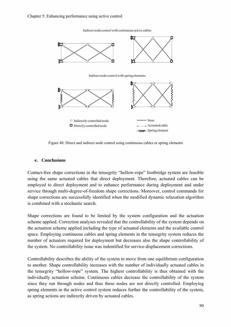
Chapter 5: Enhancing performance using active control
90
StrutActuated cableSpring element
Indirectly controlled node Directly controlled node
Indirect node control with continuous active cables
Indirect node control with spring elements
Figure 48: Direct and indirect node control using continuous cables or spring elements
e. Conclusions Contact-free shape corrections in the tensegrity “hollow-rope” footbridge system are feasible using the same actuated cables that direct deployment. Therefore, actuated cables can be employed to direct deployment and to enhance performance during deployment and under service through multi-degree-of-freedom shape corrections. Moreover, control commands for shape corrections are successfully identified when the modified dynamic relaxation algorithm is combined with a stochastic search. Shape corrections are found to be limited by the system configuration and the actuation scheme applied. Correction analyses revealed that the controllability of the system depends on the actuation scheme applied including the type of actuated elements and the available control space. Employing continuous cables and spring elements in the tensegrity system reduces the number of actuators required for deployment but decreases also the shape controllability of the system. No controllability issue was indentified for service-displacement corrections. Controllability describes the ability of the system to move from one equilibrium configuration to another. Shape controllability increases with the number of individually actuated cables in the tensegrity “hollow-rope” system. The highest controllability is thus obtained with the individually actuation scheme. Continuous cables decrease the controllability of the system since they run through nodes and thus these nodes are not directly controlled. Employing spring elements in the active control system reduces further the controllability of the system, as spring actions are indirectly driven by actuated cables.

Chapter 6: Experimental validation
Chapter 6: Experimental validation Summary: This chapter focuses on the experimental efforts performed during this thesis. The study includes two small-scale physical models of a tensegrity-ring module and a near full-scale active deployable tensegrity “hollow-rope” model. Small-scale models are easy to construct and they are useful for preliminary studies. However, they do not usually replicate all practical challenges for civil engineering applications since they do not include realistic joints and actuation devices. Therefore, a near full-scale model of the active deployable tensegrity “hollow-rope” system is designed and built. Although the behavior of the near full-scale model is affected by eccentricities in the joints, unwanted joint movements and friction, test results reveal the deployment and control potential of the system.
a. Tensegrity physical models Physical models are important for exploration, validation and development of ideas. Simple models can be used for feasibility studies as well as to identify novel solutions and challenges. Two small-scale physical models of the pentagonal tensegrity-ring module topology are thus included in this study. However, small-scale models do not usually replicate all practical challenges. Physical models of practical significance for civil engineering applications should be large enough to avoid scale-related issues and include realistic joints as well as actuation devices. Therefore, a near-full-scale model of the active deployable tensegrity “hollow-rope” system is also designed and built for this study. Tensegrity physical models are usually assumed to be easy to construct and assemble. However, their construction and assembly may be more challenging than predicted due to their spatial element arrangement and self-equilibrium state. Joint design may be another challenging task especially for deployable tensegrity systems with strut inter-connections. If the tensegrity system studied includes strut-to-strut connections, struts can serve as a reference for the assembly procedure. However, if the system has no strut interconnections (Class I tensegrity system), an assembly procedure has to be defined. Although the assembly of tensegrity systems with strut-to-strut connections may be easier to define, their joint design is more complicated compared with Class I tensegrity systems. The complexity of the joints increases further for deployable tensegrity systems with continuous cables due to the cable-sliding components. Moreover, joints are important elements of tensegrity models as they can significantly affect the behavior of the system. Elements in tensegrity systems are assumed to sustain axial loading only. Therefore, if joints include eccentricities among element connections, struts may be subject to compression and bending, thus modifying the behavior of the system.
91

Chapter 6: Experimental validation
b. Design and test of small-scale models Small-scale physical models are important for understanding and exploring tensegrity systems. The first model built is a small-scale physical model of a pentagonal tensegrity-ring module. The model is made out of wooden struts and elastic rope. Nested steel hooks are used for the strut-to-strut connections. An elastic rope is used for the tensile elements in order to compensate errors in the geometry induced by the steel hooks. Moreover, using an elastic rope allows cables to adjust their length according to the module length and therefore provides deployability to the model. The model has a length of approximately 75cm and a radius of 57cm. All struts have a diameter of 3cm and a length of 100cm. Figure 49 shows the small-scale physical model of the pentagonal tensegrity-ring-module.
Figure 49: The small-scale physical model of the pentagonal tensegrity-ring module The deployment motion and extreme values of the deployment-path space of a single pentagonal tensegrity-ring module (see Chapter 4) are validated experimentally on the small-scale physical model. As unfolding and folding are assumed to follow a similar path, folding is preferred to unfolding. Folding has been conducted manually either by applying forces on the nodes of one of the pentagonal faces or by manually changing the length of the actuated cables. Figure 50 shows the analytical deployment path space predicted by the geometrical study for the small-scale physical model and the experimental path measured on the small-scale physical model. Isometric curves reflect strut-to-strut distances and vary from 1 to 9cm (outside to inside the white region). Although steel hooks are convenient for the construction of the model, they induce errors and eccentricities that affect significantly the deployment path. Therefore, the experimental path deviates from the analytical path with folding. However, a full reversible deployment (folding and unfolding) has been achieved without strut contact, thus validating the contact-free deployment motion of the ring module.
92

Chapter 6: Experimental validation
Rotation [rad]
Model length L [cm]
0.5
0.4
0.3
0.2
0.1
0 0 20 40 60 80 100
Analytical pathExperimental path
Figure 50: The analytical and the experimental deployment-path of the small-scale physical model
The feasibility of the deployment with passive coplanar x-cables and continuous non-coplanar x-cables is also validated on the small-scale physical model of the pentagonal tensegrity-ring module (see Chapter 4). For the validation of this deployment path, the elastic rope segments of coplanar x-cables have been replaced by non-extensible nylon rope segments. The elastic rope segments of the non-coplanar x-cables have been replaced by continuous segments that run through the steel hooks. Figure 51 shows the small-scale physical model with continuous elastic and discontinuous non-extensible rope segments in its folded and unfolded configurations. A full reversible deployment (folding and unfolding) of the model has been found to be feasible without any strut contact and with passive coplanar x-cables remaining in tension as predicted.
Figure 51: Deployment snapshots of the small-scale tensegrity-ring physical model with inelastic coplanar x-cables and continuous elastic non-coplanar x-cables
93

Chapter 6: Experimental validation
Figure 52: The second-generation small-scale tensegrity-ring model In order to study deployment actuation and joint design, a second-generation small-scale physical model of a tensegrity-ring module has been designed and built. The actuation scheme of the model includes 5 continuous actuated cables and 10 spring elements (see Chapter 4). Struts are made of aluminium tubes, while steel cables and steel springs are used for the tensile elements. Figure 52 shows the second-generation small-scale physical model. Strut-to-strut joints are made of aluminium and brass based on a fork-to-fork design. The fork-joint allows sufficient element motion for deployment of the module. Moreover, the model is supported on a rail system in order to allow end motion. Figure 53 shows the fork-to-fork joint on the rail-support system. Cable-length changes in actuated continuous x-cables are controlled manually using a hand-crank system.
Figure 53: The rail-support system of the second-generation small-scale tensegrity-ring model
94

Chapter 6: Experimental validation
Although errors are induced in the system by eccentricities in the joint design (mainly due to cables), the fork-joint leads to a successful deployment of the tensegrity-ring model. Both unfolding and folding are possible without strut contact. Figure 54 shows snapshots of the deployment of the second-generation small-scale tensegrity-ring model. The deployment motion is similar to the deployment of the first physical model. Deployment is thus not affected by the use of continuous actuated x-cables and spring elements in layer cables. Deployment tests revealed that energy stored in springs during folding can be used for unfolding. Moreover, deployment has been found to be feasible with both simultaneous and sequential cable actuation. However, if sequential cable actuation is applied, the order of cable-length changes has to respect the rotational sense of the diagonal struts.
Figure 54: Deployment snapshots of the second-generation small-scale tensegrity-ring-module model with continuous actuated cables and spring elements
c. Design and test of a near-full-scale model Large-scale physical models are important when studying active deployable structures due to scale-related effects such as actuation and friction. Therefore, realistic actuation devices and joints should be employed. A near-full-scale (1/4) model of the tensegrity “hollow-rope” system with elaborate joints and motorized actuators is thus designed and built for this study. The actuation scheme with continuous actuated cables and spring elements (scheme with the minimum number of actuators required for deployment) is implemented in the model for deployment testing (see Chapter 4). The near-full-scale physical model of the tensegrity-footbridge system includes four tensegrity-ring modules (two modules per side) assembled in a linear way according to the “hollow-rope” principle (see Chapter 3). The model has a total span of approximately 5m and a diameter of approximately 0.8m. It weights approximately 100kg and is supported at both ends. The support system is based on a rail-support system that blocks longitudinal displacements allowing only the required in-plane movements for deployment (see Chapter
95

Chapter 6: Experimental validation
4). Figure 55 shows two modules of the near-full-scale active deployable tensegrity “hollow-rope” physical model.
Figure 55: The near-full-scale active deployable tensegrity “hollow-rope” physical model The model is composed of steel struts and cables selected from commercially available standard steel sections. Struts are made of hollow tube section profiles with a length of 1.35m, a diameter of 28mm and a thickness of 1.5mm. The steel grade of struts is S355 with a modulus of elasticity of 210GPa. Cables are made by stainless steel with a modulus of elasticity of 120GPa. They have a diameter of 4mm and their length varies according to their topology (layer cables, discontinuous x-cables or continuous x-cables). Strut and cable characteristics are summarized in Table 20. The spring elements employed for the deployment of the model have an initial length of 37.6mm and a stiffness of 0.9N/mm. They are connected to the joints using two chains of approximately 15cm.
Table 20: Element characteristics of the tensegrity near-full-scale physical model
Element Length [m]
Diameter [mm]
Thickness [mm]
Modulus of elasticity [GPA]
Strength [kN]
Struts 1.35 28 1.5 210 10.6
Cables * 4 - 120 9
* layer cables: 0.91m, passive x-cables: 0.69m, continuous x-cables: 2.76m The model has 25 joints per side including 5 inter-module joints and 5 support joints. The joints of the near-full-scale model are based on a fork-to-fork design similar to the second-generation small-scale model. Joint design is developed with additional components for continuous cables and for the inter-module connection. Moreover, the design has been modified to decrease eccentricities. However, a joint design without eccentricities is hard to find as element position changes in space with deployment. Figure 56 shows the CAD models of the two-strut joint with continuous cables and the four-strut inter-module connection as well as their corresponding joints on the near-full-scale physical model.
96

Chapter 6: Experimental validation
Figure 56: CAD models developed for the fork-joint design for continuous cables and inter-module connections with continuous cables and the corresponding joints on the near-full-scale physical model
The same design is applicable to all joints of the model including support joints reducing thus manufacturing costs and enhancing modularity. Although the fork-joint includes eccentricities and a large number of degrees of freedom, it allows the required element motions for the near-full-scale model to change shape. Figure 57 shows the near-full-scale model in its folded configuration.
Figure 57: The near-full-scale tensegrity “hollow-rope” model in its fully folded configuration during the assembly
97

Chapter 6: Experimental validation
The modularity of the tensegrity “hollow-rope” system is explored for the construction of the near-full-scale model. Each module of the model is pre-assembled onsite using a simple scaffolding system composed of 10 vertical supports: 5 for the nodes of the outer pentagon and 5 for the nodes of the intermediate pentagon. The strut circuit of the tensegrity-ring systems is used as reference for the assembly of the module. Once the assembly of the module is completed, the module is connected to the rest of the system. Figure 58 shows a snapshot during the modular construction of the tensegrity “hollow-rope” model and a detail regarding the joint connection among two modules. Unloaded cables show a non-linear load/elongation behavior due to their braiding geometry. Therefore, cables have been prestressed five times at 40% of their tensile strength before mounted on the system.
Figure 58: Snapshot during the modular construction of the tensegrity “hollow-rope” model and detail from the joint connection between two modules
The actuation scheme with the minimum number of actuators has been implemented for the deployment of the near-full-scale “hollow-rope” model. The model includes 5 continuous actuated cables and 15 spring elements per side (see Chapter 4). For static tests, spring elements are replaced by cables. Continuous cables are attached on the midspan nodes of the model and are controlled using an active crank system placed on the rail-support system. Figure 59 shows the active crank system on the rail-support system. The effect of the active crank system on the support nodes is limited by a weight-counterbalance system.
98

Chapter 6: Experimental validation
Figure 59: The active crank system on the rail-support system The near-full-scale model is controlled by an active control system composed of 10 actuators (5 actuators per side), an optical tracking system and a control station (PC). Actuators control the length of the continuous actuated cables and thus the shape of the model (see Chapter 4), while the optical tracking system monitors the position of the nodes of the model. Figure 60 illustrates the main components of the active control system employed in the near-full-scale physical model of the active deployable tensegrity “hollow-rope” system.
Power system
Safety test
Control station
Servomotor
Crank systemTracking system PHYSICAL MODEL Safety test
Motor driver
Figure 60: Illustration of the active control system of the near-full-scale active deployable tensegrity model Power in the active control system is provided through a central power station. However, the system remains idle until the user confirms the activation of the system (initial safety test). The user controls the stiffness and shape of the model through changes in the length of the continuous actuated cables. The lengths of continuous cables are controlled by an active crank system positioned on the support of the model avoiding thus all actuator-related constraints. The active crank system is actuated by a series of servomotors. Servomotors are common control components, known for their reliability and long-life span. They are advantageous due to their high speed response and braking ability. Furthermore, they have a wide range of positions/velocities allowing thus the model to perform small and large shape changes. A reduction gear is added to improve further the precision of the active crank system.
99

Chapter 6: Experimental validation
Servomotors are coupled with motor drivers. Motor drivers translate and transfer the commands from the control station to the servomotor. Furthermore, they allow the user to impose safety values for control commands such as maximum position or velocity in order to avoid dangerous actuation modes. Motor drivers are connected with the control station (PC) using a Control Area Network (CAN). Figure 61 shows five motor drivers of the active deployable tensegrity “hollow-rope” near-full-scale model and a snapshot of the user interface of the control-command program.
Figure 61: Motor drivers of the active deployable tensegrity “hollow-rope” large-scale model and a snapshot of
the user interface of the control-command program The active deployable tensegrity “hollow-rope” model can perform small shape corrections and large shape changes such as deployment (see Chapter 5). Therefore, traditional displacement sensors are not practical. An optical tracking system - Iotracker – is employed to monitor the shape and the displacement of the system. The Iotracker system has been developed at Vienna University of Technology. It combines two-dimensional imaging sensors (cameras) with "passive" retro-reflective markers. The real-time 6-DOF motion-tracking of the markers is obtained through geometric triangulation. The Iotracker configuration implemented in the near-full-scale model includes 8 cameras. Preliminary tests on the system revealed a precision of 0.1mm. However, long-time period tests revealed a variability of 0.5mm in results. Figure 62 shows a snapshot of the real time motion-tracking program including 8 cameras and 3 measuring points. Measuring points are illustrated as tea pots and they correspond to markers placed on midspan nodes of the near-full-scale model.
100

Chapter 6: Experimental validation
Figure 62: Snapshot of the real time motion-tracking program including the 8 cameras of the system and 3 markers (tea pots) placed on midspan nodes of the near-full-scale model
The static behavior of the tensegrity “hollow-rope” system with continuous actuated cables is studied experimentally on the near-full-scale tensegrity model. The configuration applied for static loading is a cantilever two-module system with discontinuous layer cables and continuous non-coplanar x-cables (see Chapter 3). No spring elements are employed for the static loading tests. Furthermore, all nodal displacements at the support nodes of the model are blocked. A high prestress level is applied so that results are not prestress dependent (see Chapter 3). Two load tests are performed for the static behavior of the model. The first test is conducted using a symmetric load while the second is based on an asymmetric load. Figure 63 illustrates the cantilever two-module configuration of the physical model highlighting loading position and measurement points. Displacements are measured on the lower nodes and the top node of the free end of the model.
Measurement points
Figure 63: Configuration applied for the static load tests
101

Chapter 6: Experimental validation
Figure 64: Snapshot of the near-full-scale physical model during the symmetrical load test A symmetric load test has been conducted with an incremental load of approximately 120N on the two lateral nodes of the outer pentagon of the model. Figure 64 shows a snapshot of the near-full-scale model with discontinuous and continuous cables during the symmetrical loading test. Figures 65 to 67 show the relative displacements measured on the three nodes of the near-full-scale physical model and their corresponding analytical values. The displacements of the analytical model are estimated using the modified dynamic relaxation algorithm (see Chapter 3). The two models show a similar and almost linear behavior. However, displacements measured on the physical model are smaller compared with the displacements given by the analytical model. Consequently, the near-full-scale physical model is stiffer than predicted. This is most likely due to the joint friction which is not considered in the analytical model.
0
200
400
600
800
1000
0 0.5 1 1.5 2 2.5
3
Series1Series2
Force [N]
Analytical modelPhysical model
Relative displacement on the vertical axis [cm]
Figure 65: Relative vertical displacements on the lower-left node of the near-full-scale model under symmetrical
loading
102

Chapter 6: Experimental validation
0
200
400
600
800
1000
0.0 0.5 1.0 1.5 2.0 2.5 3.0
Series1
Series2
Force [N]
Analytical modelPhysical model
Relative displacement on the vertical axis [cm]
Figure 66: Relative vertical displacements on the lower-right node of the near-full-scale model under symmetrical loading
0
200
400
600
800
1000
0 0.5 1 1.5 2 2.5
3
Series1Series2
Force [N]
Analytical modelPhysical model
Relative displacement on the vertical axis [cm]
Figure 67: Relative vertical displacements on the top node of the near-full-scale model under symmetrical
loading The asymmetric loading test has been conducted with an incremental load of approximately 120N on the lateral-left node of the outer pentagon of the model (Figure 63). Figures 68 to 70 show the relative displacements measured on three nodes of the near-full-scale physical model and their corresponding analytical values obtained with the modified dynamic relaxation algorithm (see Chapter 3). Similar to the symmetric loading test, the two models show a similar and almost linear behavior with a higher stiffness (lower displacements) for the physical model due to joint friction. The difference in displacements between the analytical and the physical model in Figure 68 is due to an unwanted joint motion that occurs under loading. A similar effect is observed for the last measurement of Figure 70.
103

Chapter 6: Experimental validation
0
100
200
300
400
500
0 0.25 0.5 0.75 1 1.25 1.5 1.75 2
Series1Series2
Force [N]
Analytical modelPhysical model
Relative displacement on the vertical axis [cm]
Figure 68: Relative vertical displacements on the lower-left node of the near-full-scale model under
asymmetrical loading
0
100
200
300
400
500
0 0.25 0.5 0.75 1 1.25 1.5 1.75 2
Series1Series2
Force [N]
Analytical modelPhysical model
Relative displacement on the vertical axis [cm]
Figure 69: Relative vertical displacements on the lower-right node of the near-full-scale model under
asymmetrical loading
104

Chapter 6: Experimental validation
0
100
200
300
400
500
0 0.25 0.5 0.75 1 1.25 1.5 1.75 2
Series1Series2
Force [N]
Analytical modelPhysical model
Relative displacement on the vertical axis [cm]
Figure 70: Relative vertical displacements on the top node of the near-full-scale model under asymmetrical
loading In order to study the load-sequence sensitivity of the near-full-scale model, static tests with inversed load sequences have been performed. An incremental load of approximately 240N has been applied on the left lateral node of the outer pentagon of the model before being applied on the right lateral node (load sequence I). For load sequence II, the sequence has been inversed with the right lateral node loaded first. Figures 71 to 73 show the relative displacements measured on the three nodes of the near-full-scale physical model for the two load sequences. Although displacements reveal a similar and almost linear behavior, final displacements under the same load differ for the two sequences. Consequently, load sequence has to be considered in the analysis method.
0
200
400
600
800
1000
0.0 0.8 1.5 2.3 3.0 3.8 4.
5
Series1Series2
Force [N]
Load sequence ILoad sequence II
Relative displacement on the vertical axis [cm]
Figure 71: Relative vertical displacements on the lower-left node of the near-full-scale model for two load
sequences
105

Chapter 6: Experimental validation
0
200
400
600
800
1000
0.0 0.8 1.5 2.3 3.0 3.8 4.5
Series1Series2
Force [N]
Load sequence ILoad sequence II
Relative displacement on the vertical axis [cm]
Figure 72: Relative vertical displacements on the lower-right node of the near-full-scale model for two load sequences
0
200
400
600
800
1000
0.0 0.8 1.5 2.3 3.0 3.8 4.5
Series1Series2
Force [N]
Load sequence ILoad sequence II
Relative displacement on the vertical axis [cm]
Figure 73: Relative vertical displacements on the top node of the near-full-scale model for two load sequences The behavior of the tensegrity “hollow-rope” system under control has been studied on the near-full-scale model. Relative vertical displacements are estimated using an experimentally actuation-sensitivity matrix and the modified dynamic relaxation algorithm and compared with displacement measured on the physical model. Figures 74 and 75 show the relative displacements measured on three nodes of the near-full-scale physical model for two actuation tests and their corresponding analytical values obtained using the actuation-sensitivity matrix and the modified dynamic relaxation algorithm. Although values for the sensitivity matrix have been determined through unitary actuations on the physical model, displacement direction is not correctly predicted. This is likely due to the competing effect of single actuation versus multiple actuations which is not taken into account in the sensitivity
106

Chapter 6: Experimental validation
matrix. Dynamic relaxation predicts better the behavior of the model. However, displacement magnitude is not correctly predicted and this is most likely due to the joint friction.
-8
-6
-4
-2
0
2
4
6
8
1 2 3
Series1
Series2
Series3
Sensitivity matrixDynamic relaxationMeasured value
Relative displacement on the vertical axis [cm]
Node number
Figure 74: Analytical and experimental relative vertical displacements measured of three nodes of the near-full-
scale model for actuation test I
-8
-6
-4
-2
0
2
4
6
8
1 2 3
Series1Series2Series3
Sensitivity matrixDynamic relaxationMeasured value
Relative displacement on the vertical axis [cm]
Node number
Figure 75: Analytical and experimental relative vertical displacements measured of three nodes of the near-full-
scale model for actuation test II The feasibility of the deployment and control of the tensegrity “hollow-rope” system with continuous actuated cables and spring elements has been studied experimentally on the near-full-scale active deployable tensegrity model (see Chapter 4). Cable-length changes are directed by the control station through the active crank system while the shape of the model (nodal positions) is monitored by the optical tracking system. The same actuation step has been applied to all actuated cables (see Chapter 4). Figure 76 shows a series of snapshots of the deployment motion of the near-full-scale active deployable tensegrity model. The
107

Chapter 6: Experimental validation
deployment motion of the near-full-scale model is similar to the geometrical model including a translation, a rotation and a dilation (see Chapter 4). However, folding is limited to approximately 50% of its deployed length due to eccentricities in the joints, unwanted joint movements and friction.
108

Chapter 6: Experimental validation
Figure 76: Snapshots of the deployment motion of the near-full-scale active deployable tensegrity model
109

Chapter 6: Experimental validation
The near-full-scale model has been designed based on a reticulated strut-cable model, where joints are assumed to be frictionless pin-jointed connections. Consequently, only axial forces are taken into account in the structural analysis. Although the fork-joint design has been modified to decrease eccentricities among elements, struts are subject to bending as folding increases. This appearance is likely due to the large scale of the model and the applied deployment-actuation scheme as spring elements elongated with folding. Such increasing forces in the model thus highlight the existence of eccentricities in the joints through an elastic bending-deformation mode in struts. Consequently, the risk of failure due to compression and bending increases with folding. Failure may however be avoided through modifying the joints to decrease eccentricities and through considering eccentricities in the structural analysis and consequently, replacing elements. Although friction in the near-full-scale model has been reduced with the use of special materials in contact surfaces such as Polytetrafluoroethylene (PTFE) and Polyoxymethylene (POM), deployment motion is found to be significantly influenced by friction. The main assumption for the deployment of the “hollow-rope” system is that all nodes in the system follow a similar deployment path. Figure 77 shows the deployment paths (length, rotation) of three midspan nodes of the near-full-scale active deployable tensegrity model during deployment (folding and unfolding). Although the nodes follow similar paths for folding and unfolding, the relative rotation is not the same for the three nodes. Furthermore, their path is not similar to the analytical path obtained from the geometrical analysis. Consequently, the regularity of the pentagonal tensegrity-ring module is lost limiting thus the deployability of the system. Figures 78 and 79 reveal a similar effect on the relative displacements of the three midspan nodes. The deployment paths of the nodes may be corrected using spring elements with a higher stiffness or through individual actuation steps (shape corrections).
0
0.2
0.4
0.6
0.8
1
0 20 40 60 80
100
Series4Series2Series1Series3
Relative rotation [rad]
Analytical modelMidspan top nodeMidspan lower-left nodeMidspan lower-right node
Relative displacement on the longitudinal axis [cm]
Figure 77: Relative rotation of three midspan nodes during the deployment motion (folding and unfolding) of the
near-full-scale active deployable tensegrity model
110

Chapter 6: Experimental validation
-50.0
-30.0
-10.0
10.0
30.0
50.0
0.0 20.0 40.0 60.0 80.0 100.0
Series2Series1
Series3
Relative displacement on the longitudinal axis [cm]
Midspan top nodeMidspan lower-left nodeMidspan lower-right node
Relative displacement on the vertical axis [cm]
Figure 78: Relative vertical displacements of three midspan nodes during the deployment motion (folding and unfolding) of the near-full-scale active deployable tensegrity model
-60.0
-40.0
-20.0
0.0
20.0
40.0
60.0
0.0 20.0 40.0 60.0 80.0 100.0
Series2
Series1
Series3
Relative displacement on the lateral axis [cm]
Midspan top nodeMidspan lower-left nodeMidspan lower-right node
Relative displacement on the longitudinal axis [cm]
Figure 79: Relative lateral displacements of three midspan nodes during the deployment motion (folding and unfolding) of the near-full-scale active deployable tensegrity model
d. Conclusions The experimental tests conducted on physical models validate the feasibility of an active deployable tensegrity “hollow-rope” footbridge system. The contact-free deployment path and the continuous-spring actuation scheme are successfully validated using small-scale physical models. Furthermore, it has been found that energy stored in springs during folding can be used for unfolding.
111

Chapter 6: Experimental validation
112
A similar deployment motion is observed on the near-full-scale model where the shape of the model is controlled by an active crank system and an elaborate joint design is employed. However, the deployment-shape transformation of the near-full-scale active model is limited by eccentricities in the joints, unwanted joint movements and friction. Joints affect also the static behavior of the near-full-scale model as the displacements measured on the model are usually smaller than predicted by the analytical model. However, the behavior of the system is correctly reflected.

Chapter 7: Conclusions
Chapter 7: Conclusions Summary: Research challenges, assumptions and methodology are discussed in this chapter. Main results and conclusions are drawn from each chapter. Finally, ideas for further research and development are presented. Transferability of results is also discussed.
a. Discussion This thesis investigates an active deployable tensegrity “hollow-rope” footbridge as an example of an active civil engineering structure. Active structures adapt to environmental changes, load modifications or eventual partial failure using an integrated actuator-sensor system. In this study, active control has been used to control large shape transformations such as deployment and small transformations such as shape corrections before, during and after deployment (in service). Deployment, its actuation schemes and their influence in structural design have been studied numerically. Moreover, the feasibility of the active deployable tensegrity system has been shown experimentally with the study of a near-full-scale physical model. The thesis has been guided by the following scientific question (presented in Chapter 1):
Is a deployable tensegrity “hollow-rope” footbridge feasible? If yes, can active elements be employed to control and improve shape transformations (including deployment and shape corrections) and in-service performance?
and its related objectives:
a. Study the deployment of the tensegrity-footbridge system: numerically and experimentally
b. Design an active control system to ensure the deployment of the tensegrity system
c. Study the tensegrity structure in service (after deployment)
d. Design an active control system to ensure serviceability of the tensegrity footbridge
e. Construction and analysis of a near full-scale physical model of the tensegrity-footbridge system
113

Chapter 7: Conclusions
To fulfill the above objectives the following challenges had to be overcome during the thesis:
• In order to study tensegrity systems with continuous cables and spring elements under service and during deployment an appropriate analysis method is required since cable continuity changes tensegrity mechanics. Therefore, the dynamic relaxation algorithm has been modified to include cable continuity.
• There are no globally accepted design guidelines for tensegrity structures in civil engineering. Therefore, the design of the tensegrity “hollow-rope” footbridge system has been guided by parametric analyses and advanced computing methods.
• In order to study the structural behavior of the tensegrity-footbridge system during the deployment an appropriate numerical analysis method is required. An algorithm that integrates actuation schemes along with the modified dynamic relaxation algorithm has been used under the assumption of pin-jointed connections, frictionless motions and quasi-static actuation.
• Since there are no globally accepted design guidelines for active structures, active control systems are related to specific applications and contexts. For the deployment of the tensegrity “hollow-rope” footbridge system, actuation schemes (including actuator placement and action) have been identified. Therefore, the design of the active control systems has been guided by geometrical, numerical and physical models. Control commands have been identified using stochastic search.
• Finally, valid physical models require appropriate joint designs that induce a minimum error such as those caused by joint eccentricities. Joints must allow the required motions to the system while providing sufficient strength. Joint requirements may thus be in conflict as both strength and eccentricities increases with size. Moreover, it is preferable if the joint design is universal thus remaining applicable for all type of connections in the system (including two or four strut connections with discontinuous or continuous cables).
Results of this thesis are based on three main assumptions. First, elements of the active deployable tensegrity “hollow-rope” footbridge system are assumed numerically to be linked with pin-jointed connections. Second, continuous cables are modeled numerically to run without friction through the nodes. Deployment is thus assumed to be conducted simultaneously for all modules in the system. Finally, quasi-static actuation and frictionless motion are assumed for simulations of shape transformations. The deployable tensegrity system studied is a spatial reticulated strut-cable structure. Joints are thus assumed to be pin-jointed connections and therefore only axial forces are taken into account in the structural analysis. Finding a joint design with no eccentricities for all elements including the continuous sliding cables and for all shape configurations resulted in unpractical designs. A joint design based on a rotational fork-to-fork principle that satisfies the required motion has been developed. Consequently, deviations from the predicted behavior of the
114

Chapter 7: Conclusions
structure have been observed in the experimental validation due to eccentricities in the joints, unwanted joint movements and friction.. Quasi-static actuation and frictionless motion have been assumed for shape transformations of the deployable tensegrity-footbridge system. Quasi-static actuation guarantees that acceleration and velocity terms in the deployment analysis can be neglected. Consequently, the dynamic analysis of the deployment can be approximated by static analyses that thus can be conducted using the dynamic relaxation method. Experimentally this is obtained with a low actuation speed (deployment time is 100 times larger than the period of the first natural frequency of the system). If element-length variations are conducted in high speed (dynamic actuation), acceleration and velocity have to be taken into account in the analysis and other methods such as rigid body dynamics have to be applied. Finally, experimental validation is also influenced by joint friction. However, joint friction in physical models has been reduced with the use of special materials in contact surfaces such as Polytetrafluoroethylene (PTFE) and Polyoxymethylene (POM).
b. Conclusions Conclusions of this thesis contribute towards the development of active tensegrity structures that are capable of complex multiple-degree-of-freedom shape transformations, thereby, extending the boundaries of active and bio-mimetic structures. Main results and conclusions drawn from them are grouped according to subtopics addressed and they are detailed in the next subsections. Structural analysis The structural analysis of the tensegrity “hollow-rope” system has been conducted using the dynamic relaxation method under the assumption of a pin-jointed structure. In the absence of globally accepted design guidelines for tensegrity structures, a design methodology based on parametric studies has been proposed and stochastic search has been applied for the design of the tensegrity “hollow-rope” footbridge system. Both methods generate designs that satisfy safety and serviceability criteria. However, stochastic search provides design solutions with significantly lower cost. Additionally, it can support a range of “what-if” analyses since engineers can easily modify the objective function to accommodate additional constraints. The following conclusions are drawn from structural analyses:
• Structural analyses revealed the importance of the level of self-stress as a design parameter. Design solutions obtained through material cost minimization have relatively high self-stress level thus increasing labor costs. This justifies explicitly taking into account self-stress costs in order to ensure a consistent design solution of the tensegrity system.
115

Chapter 7: Conclusions
• A key parameter for the structural behavior of the system is the stiffness ratio between cables and struts. Increasing this ratio decreases vertical displacements until reaching a limit that varies according to material properties. In the lack of globally accepted design guidelines, a design methodology similar to tensegrity-grid guidelines has been proposed based on the stiffness ratio between cables and struts.
• Employing continuous cables changes significantly the mechanics of tensegrity structures and consequently affects design solutions. The dynamic relaxation algorithm has been modified to include cable continuity. Design solutions with both discontinuous and continuous cables that satisfy safety and serviceability criteria have been found for the tensegrity “hollow-rope” footbridge-system. The continuous design solution has larger cross-section areas compared with the discontinuous configuration.
• Eigen-frequency analysis results showed that the fundamental frequency of the tensegrity “hollow-rope” footbridge is not directly influenced by the self-stress level. This is due to the absence of infinitesimal mechanisms in the tensegrity “hollow-rope” system. However, natural frequencies are influenced by design parameters such as the cross-sectional area of cables. Consequently, dynamic behavior requirements have been introduced as an additional criterion in the design process of the tensegrity-footbridge system. Design solutions with both discontinuous and continuous cables that satisfy safety and serviceability criteria as well as dynamic requirements have been found for the tensegrity-ring footbridge-system.
• Employing discontinuous and/or continuous cables changes the design solution for the tensegrity “hollow-rope” structure. Structural analyses revealed that the design of the tensegrity-footbridge system is governed by static requirements for configurations with discontinuous cables only and by dynamic requirements for configurations with continuous cables.
These results underline the complexity of the design of tensegrity structures and the advantages of employing advanced computing methods. They also reveal that tensegrity structures such as the tensegrity “hollow-rope” system are viable systems for civil engineering applications if properly designed. Deployment analysis The deployment of the tensegrity “hollow-rope” system was studied combining geometrical models, numerical models and physical models. Geometrical models were used as reference for deployment, while physical models were used to explore and validate actuation aspects. The deployment analysis of the tensegrity” hollow-rope” system was conducted using an algorithm that combines actuation with the modified dynamic relaxation algorithm under the assumptions of a quasi-static actuation and frictionless motion.
116

Chapter 7: Conclusions
The following conclusions are drawn from the deployment analysis:
• Contact-free deployment of the tensegrity-ring system is feasible using cable control. The deployment-path space for the contact-free deployment has been found through strut-to-strut distance calculations. Furthermore, the deployment path with the minimum strut-contact risk and the deployment path with the minimum number of cable-length changes (actuators) have been identified through exploring the path space.
• The structural behavior of the tensegrity system during deployment was analyzed using a dynamic-relaxation-based algorithm. Cable-length changes are applied to create finite mechanisms that allow the module to change length and to find new equilibrium configurations. Consequently, the deployment path is composed of a series of intermediate equilibrium configurations. Consequently, the system remains stiff during deployment without requiring any external elements. The size of the actuation-step has been identified as a critical parameter for deployment. Large steps result in unstable configurations, while small steps are computationally expensive.
• The number of cable-length changes and consequently actuators required for deployment depends on the path followed and the actuation scheme applied. Continuous cables and spring elements can be used to reduce the number of actuators. However, actuation schemes with continuous cables and spring elements affect the structural behavior of the system.
• If only actuated cables - discontinuous and/or continuous - are employed in the tensegrity structure, deployment is not a critical design case. However, a large number of actuators is required in the system. Actuator-related design-constraints may thus become critical for the design.
• Deployment is the critical design case when spring elements are integrated in the actuation scheme of the tensegrity “hollow-rope” system. If spring characteristics are defined to satisfy safety and serviceability criteria as well as dynamic requirements, then element sizing increases significantly. If spring characteristics are defined based only on the deployment case, safety and dynamic requirements can be met but excessive vertical displacements may occur under service. However, employing spring elements decreases significantly the number of actuators thus reducing or even eliminating actuator-related constraints.
These results highlight the efficiency of cable controlled tensegrity systems for deployable applications since they can remain in equilibrium and thus stiff throughout deployment without requiring any additional stabilization elements. Furthermore, results underline the importance of including deployment and actuation schemes along with traditional design cases when designing deployable tensegrity structures as they may significantly affect design solutions.
117

Chapter 7: Conclusions
Structural control Active cables can be employed to direct the deployment of the tensegrity “hollow-rope” system as well as to enhance deployment and service performance through multi-degree-of-freedom shape corrections. Shape corrections have been studied using a dynamic-relaxation-based algorithm under the assumptions of a quasi-static actuation and frictionless motions. Considering the complex behavior of the tensegrity “hollow-rope” footbridge system, a single objective stochastic algorithm has been used to find good control commands. The following conclusions are drawn from the structural control study:
• Deployment can be enhanced through contact-free shape corrections of the deployed configuration using the same actuation schemes that direct the deployment-shape transformation. Control commands for shape corrections are successfully identified when the modified dynamic relaxation algorithm is combined with a stochastic search algorithm. However, shape corrections are limited by the system configuration and the actuation scheme applied (controllability issue).
• Service can be enhanced through contact-free displacement corrections of the service configuration using the same actuation schemes that direct the deployment-shape transformation. The deployment-actuation schemes of the tensegrity system with individually actuated cables, continuous actuated cable and spring elements were found to be able to successfully direct deployment and correct midspan displacements under service. No controllability issue was indentified for service-displacement corrections. Control commands for displacement corrections are successfully identified when the modified dynamic relaxation algorithm is combined with a stochastic search algorithm.
• Deployment-actuation schemes are less efficient regarding shape corrections during deployment mainly due to controllability issues. Correction analyses revealed that the controllability of the system depends on the actuation scheme applied including the type of actuated elements and the available control space. Controllability describes the ability of the system to move from one equilibrium configuration to another. Shape controllability increases with the number of individually actuated cables in the tensegrity “hollow-rope” system. The highest controllability is thus obtained with the individually actuation scheme. Continuous cables decrease the controllability of the system since they run through nodes and thus these nodes are not directly controlled. Employing spring elements in the active control system reduces further the controllability of the system, as spring actions are indirectly driven by actuated cables.
These results show that active control can improve the quality of deployment and in-service performance. Furthermore, they reveal the complexity of the shape control of tensegrity structures, especially when continuous cables and springs are employed due to indirect control, and thus the advantages of employing advanced computing methods.
118

Chapter 7: Conclusions
Experimental study The experimental study on the active deployable tensegrity system included physical models at various scales. Physical models were studied for feasibility purposes as well as investigation and validation of results in combination with analytical models. Small-scale models have been used for exploration, validation and development of ideas. However, small-scale models do not usually replicate all practical challenges. Therefore, a near-full-scale model of the tensegrity “hollow-rope” system with realistic joints as well as actuation devices has been also designed and built for this study. The following conclusions are drawn from the experimental study:
• Experimental tests conducted on small-scale and large-scale physical models validate the feasibility of an active deployable tensegrity “hollow-rope” footbridge system. The proposed actuation schemes can direct both large shape transformations such as deployment and small shape corrections.
• The contact-free deployment path and the continuous-spring actuation scheme are successfully validated using small-scale physical models. Furthermore, it has been found that energy stored in springs during folding can be used for unfolding.
• A similar deployment motion is observed on the near-full-scale model where the shape of the model is controlled by an active crank system and an elaborate joint design is employed. However, the deployment-shape transformation of the near-full-scale active model is limited by eccentricities in the joints, unwanted joint movements and friction.
• Although joints affect also the static behavior of the near-full-scale model as the displacements measured on the model are usually smaller than predicted by the analytical model, the behavior of the system is correctly reflected.
These results underline the importance of combining analytical models with large-scale physical models in the development of novel active deployable structures. Physical models reveal important challenges such as joint design for the application of active deployable tensegrity systems in construction or aerospace engineering. Finally, although the results on near-full-scale model are limited by eccentricities in the joints, unwanted joint movements and friction, they highlight the potential of the active deployable tensegrity system.
c. Future work During this work, many ideas have emerged. Ideas discussed in this section include both enhancements and new research directions. Additionally, studies that aim to remove scope limitations are discussed.
119

Chapter 7: Conclusions
System topology
• Class I The tensegrity “hollow-rope” system that is employed for the active deployable tensegrity-footbridge application includes Class II and Class IV strut-to-strut joints. Strut connectivity and cable continuity increase significantly the complexity of the joints and thus the cost of the structure. Therefore, Class I tensegrity topologies require a more extensive study as they may have a lower cost due to a simpler joints. In this study, no overlap is considered among the linearly connected Class I modules. Consequently, Class I modules have been found to be far more flexible than Class II modules. Appropriate Class I topologies with the right overlap among modules may reveal similar or higher structural performance compared with the Class II modules under a lower cost. Structural analysis
• Spring elements Employing continuous cables and spring elements on the tensegrity “hollow-rope” system provides advantageous configurations for shape control. Continuous cables and spring elements change the distribution of internal forces and decrease the overall stiffness of the system. However, they can be used to reduce the number of cables to control. In this study, the influence of spring elements in the structural behavior focuses on their stiffness assuming a fixed initial spring length. Spring characteristics can be further optimized considering structural performance and length changes required for self-stress and/or during shape changes. Furthermore, spring-damping devices can also be employed in the system.
• Load sequences and dynamic loading Structural analysis shows that the tensegrity “hollow-rope” system is viable for the proposed footbridge application. However, the system has been found to be sensitive to load-application sequences. Although multiple loads have been considered in the structural analysis, the effect of the load-application sequence has not been examined. Therefore, load scenarios should also be studied considering various application sequences. Structural analysis was performed under static loading. Dynamic loads such as wind and pedestrians as well as their corresponding effects that were not taken into account in this study should be investigated.
• Analysis methods The structural analysis of the active deployable tensegrity “hollow-rope” footbridge is performed using the dynamic relaxation method based on a reticulated strut-cable model,
120

Chapter 7: Conclusions
where joints are assumed to be frictionless pin-jointed connections. Consequently, only axial forces are taken into account in the structural analysis. However, joint eccentricities are hard to avoid especially for deployable systems. Therefore, other methods such as the finite element method should also be employed in order to study the effect of various joint designs in the behavior of the model.
• Damage tolerance Tensegrity structures can be damage tolerant systems as multiple internal force distributions may be available. The degree of damage tolerance depends to the topology and to the design solution applied. Therefore, the degree of damage tolerance of the tensegrity “hollow-rope” system should be studied identifying cases of local damage and progressive collapse. Damage-tolerance studies should include both partial damage and sudden element failure. Aspects such as post-buckling behavior of struts and plastic behavior of cables should be investigated. Sudden element failure should also be studied due to the self-equilibrated prestress state of the tensegrity system. In that case, dynamic analysis should be employed as the structure will oscillate before reaching a new equilibrium or fail. Deployment analysis
• Actuation schemes The proposed actuation schemes allow the deployment of the structure. However, actuation schemes employing cables that run in parallel with other cables (multiple-cable routed strategy) or spring elements may provide a better control of the shape of the system and should be thus investigated. The number and position of the actuated cables will affect the deployability, the controllability and the robustness of the system.
• Closed-form solution Deployment has been studied through a series of static equilibrium configurations. Intermediate equilibrium configurations depend on the actuation steps applied. However, it would be to interesting to study the closed-form solution of equilibrium manifold as it may provide a better understanding of the behavior of the system and improve the shape control.
• Deployment-step optimization Deployment has been studied using the same actuation steps in all active cables. Although the use of a single deployment-step simplifies deployment control, it also limits its shape control during deployment. Therefore, differential deployment steps should be explored. Moreover, deployment steps can be optimized for segments of the deployment path.
121

Chapter 7: Conclusions
• Multi-objective control Deployment-actuation steps are found based on geometrical and structural analyses. If a perturbation occurs, the system may deviate significantly from its deployment path and problematic configurations may occur. Actuation steps that correct the trajectory of the system are found using a single objective stochastic search algorithm. Actuation-step search can be enhanced to include multiple objectives and deployment-operation criteria such as minimization of the number of correction-steps and flexibility for future transformations.
• Dynamic actuation In this thesis, deployment analysis has been subject to quasi-static actuation limitation. Deployment has been thus studied through a series of static equilibrium configurations with different system lengths. If dynamic actuation is assumed, static results are no longer valid. Deployment with dynamic actuation should thus be studied using methods that taken into account velocity and acceleration terms such as rigid body dynamics.
• Damage tolerance The degree of damage tolerance in the tensegrity system during deployment depends mainly on the control strategy applied. Therefore, damage tolerance should be studied with respect to the actuation scheme applied identifying cases that lead to deployment failure and/or collapse of the structure. Damage scenarios for deployment should include both passive and active element failure examining both partial damage and sudden element failure cases. Structural control
• Actuation schemes
The proposed actuation schemes have been conceived to direct the deployment of the structure. Therefore, they are less efficient regarding shape corrections. However, the proposed schemes can be modified to include shape corrections. Similar to deployment control, actuation schemes exploring cables that run in parallel with other cables (multiple-cable routed strategy, see Chapter 2) or spring elements can also be investigated. The number and position of active cables will affect the controllability and the robustness of the system.
• Spring elements
The efficiency of the actuation scheme employing continuous actuated cables and spring elements is significantly affected by spring characteristics. Therefore, optimizing spring characteristics may result in a better shape control of the tensegrity system.
122

Chapter 7: Conclusions
• Control enhancement Control commands for shape corrections are successfully identified when the modified dynamic relaxation algorithm is combined with a stochastic search algorithm. However, active control can be enhanced using advanced computing methods. Computing methods such as case-base reasoning may improve structural control through reducing computational time as well as through increasing accuracy and robustness of the control.
• Multi-objective control Similar to deployment control, structural control commands are found using a single objective stochastic search method. Therefore, control-command search can be enhanced including multiple objectives and operation criteria for shape corrections such as minimization of the number of correction-steps and flexibility for future transformations.
• System identification The initial state of the system is important for the identification of good control commands. Therefore, in order to correctly identify the current state of the structure sensor placement should be studied considering service and deployment criteria. Moreover, sensors can be coupled with small movements induced by the actuators for damage-identification studies.
• Damage compensation In this work, active elements have been applied for deployment and serviceability purposes. However, they can be also further employed for damage compensation. In case of local damage in the system, high internal forces and excessive displacements may occur. Active control can be employed to reduce internal forces and displacements to acceptable levels. The damaged structure may thus continue to satisfy safety and serviceability criteria. Experimental work
• Load scenarios and control space Results of tests carried out on the near full-scale tensegrity-footbridge model reveal the feasibility of the active deployable tensegrity system. However, these tests reflect only a small set of the possible loading scenarios and thus cannot be used to define control commands. Therefore, more tests should be carried out using both static and dynamic loads. Moreover, tests should also be performed on the four-module configuration of the model.
123

Chapter 7: Conclusions
• Joint design Joints are critical for the behavior and performance of tensegrity models especially for transformable systems with large shape changes. The joints of the near-full-scale physical model allow the required movements for the deployment of the active deployable model. However, the performance of the model is limited by eccentricities in the joints, unwanted joint movements and friction. Consequently, the actual behavior of the deployable tensegrity system deviates from the predicted behavior. Therefore, joints should be further studied to decrease/eliminate errors.
• Actuation schemes
Deployment-test results of the near-full-scale model reveal that the two modules of the model do not follow the same deployment path. This may be avoided employing cables that run in parallel with other cables (multiple-cable routed strategy) on the first module assuring thus the same deployment path for the two modules. Therefore, multiple-cable routed actuation schemes should be explored.
• Monitoring system Since joints affect the behavior of the system inducing bending in struts, it would be interesting to evaluate this effect through the placement of strain gauges on the struts. Strain gauges can also be employed to enhance control by a better identification of the initial state of the physical model. Furthermore, they can also be used for tests under a multi-objective control of the system as well as for damage-tolerance tests.
• Control enhancement The deployment of the model is limited by eccentricities in the joints, unwanted joint movements and friction. Consequently, control commands may also not have the predicted results when applied on the model. Feedback control should be used to assure that control commands are successfully applied enhancing thus the control of the model. Moreover, in order to correct errors induced by joints in the control algorithm advanced computing methods such as neural networks could be employed, see for example Domer et al. (2003).
d. Transferability of results This thesis investigates a deployable tensegrity footbridge as an example of an active civil engineering structure. However, the methodology and algorithms used for the tensegrity “hollow-rope” system remain valid for other civil engineering applications, disciplines and scales.
124

Chapter 7: Conclusions
The design methodology proposed and the analysis algorithms are valid for other tensegrity systems and civil engineering applications. Similar to the tensegrity “hollow-rope” footbridge studied in this thesis, a spindle-tensegrity footbridge with a 32m span was proposed for a design competition in Prato (Italy) in cooperation with the architecture office “Blue Office Architecture”, Bellinzona (Switzerland). Appendix G shows the spindle-tensegrity footbridge system. Additionally, a tensegrity dome made of wood struts and steel cables was proposed for a shelter application in the Wood Award 2012 design competition. Both structures were designed using the methodology and algorithms developed in the context of this thesis. This thesis investigates the application of the tensegrity “hollow-rope” system in civil engineering. Therefore, this work focuses on a large scale application such as the tensegrity footbridge. However, tensegrity systems have also been used in other disciplines at smaller scales such as biology where they have been used to model the behavior of structures such as a cellular cytoskeleton. The algorithms proposed for the analysis of the deployable tensegrity “hollow-rope” system can thus be used to analyze tensegrity models of biological structures.
125

Chapter 7: Conclusions
126

Appendixes
Appendix A: Analysis of a simplex module according to the generalized equilibrium-matrix formulation
This section presents an example of tensegrity mechanics according to the generalized formulation described in the article “Investigation of Clustered Actuation in Tensegrity Structures” by Moored, K.W. and Bart-Smith, H (2009). The three struts and nine cables simplex module shown in Figure 80 is used for this example.
Figure 80: Illustration of the simplex tensegrity module
1. Vector of nodal point positions
p∈R3n×1 is a vector of the nodal point positions in [cm], where n is the number of nodes in the structure. For a Cartesian coordinate system p = [p1 p2 … pn]T = [x1 y1 z1 x2 y2 z2 … xn yn zn]. The vector of nodal points p for the simplex module is: p =
100 0 0
-50 86.6
0 -50
-86.6 0
-86.6 50 200 0
-100 200 86.6 50 200
127

Appendixes
2. Element identifier vector
z∈Re×1 is an element identifier vector where, e, is the number of elements and zi = 1 if element is a cable or zi = -1 if element is a strut. The element identifier vector for the simplex module (3 struts and 9 cables) z is: z =
-1 -1 -1 1 1 1 1 1 1 1 1 1
3. Connectivity matrix
C1∈Rn×e is a matrix parameterization of the element set of a tensegrity structure that defines the element-node connectivity:
1
if the element starts from node j if the element terminates at node j
0 otherwise
i
ji i
zC z
⎧⎪= −⎨⎪⎩
[Eq. A1]
The connectivity matrix C1 for the simplex module is: C1 =
1 0 0 1 0 -1 0 0 0 1 0 0 0 0 1 -1 1 0 0 0 0 0 0 1 0 1 0 0 -1 1 0 0 0 0 1 0
-1 0 0 0 0 0 1 0 -1 0 0 -1 0 0 -1 0 0 0 -1 1 0 0 -1 0 0 -1 0 0 0 0 0 -1 1 -1 0 0
The connectivity matrix C can be extended C∈R3n×3e and C=C1 ⊗Id, where is the Kronecker ⊗tensor product and Id is an identity matrix of size d which is the dimension of the space.
128

Appendixes
The extended connectivity matrix C for the simplex module studied after the application of the Kronecker tensor product is: C =
1 0 0 0 0 0 0 0 0 1 0 0 0 0 0 -1 0 0 0 0 0 0 0 0 0 0 0 1 0 0 0 0 0 0 0 00 1 0 0 0 0 0 0 0 0 1 0 0 0 0 0 -1 0 0 0 0 0 0 0 0 0 0 0 1 0 0 0 0 0 0 00 0 1 0 0 0 0 0 0 0 0 1 0 0 0 0 0 -1 0 0 0 0 0 0 0 0 0 0 0 1 0 0 0 0 0 00 0 0 0 0 0 1 0 0 -1 0 0 1 0 0 0 0 0 0 0 0 0 0 0 0 0 0 0 0 0 0 0 0 1 0 00 0 0 0 0 0 0 1 0 0 -1 0 0 1 0 0 0 0 0 0 0 0 0 0 0 0 0 0 0 0 0 0 0 0 1 00 0 0 0 0 0 0 0 1 0 0 -1 0 0 1 0 0 0 0 0 0 0 0 0 0 0 0 0 0 0 0 0 0 0 0 10 0 0 1 0 0 0 0 0 0 0 0 -1 0 0 1 0 0 0 0 0 0 0 0 0 0 0 0 0 0 1 0 0 0 0 00 0 0 0 1 0 0 0 0 0 0 0 0 -1 0 0 1 0 0 0 0 0 0 0 0 0 0 0 0 0 0 1 0 0 0 00 0 0 0 0 1 0 0 0 0 0 0 0 0 -1 0 0 1 0 0 0 0 0 0 0 0 0 0 0 0 0 0 1 0 0 0
-1 0 0 0 0 0 0 0 0 0 0 0 0 0 0 0 0 0 1 0 0 0 0 0 -1 0 0 0 0 0 0 0 0 -1 0 00 -1 0 0 0 0 0 0 0 0 0 0 0 0 0 0 0 0 0 1 0 0 0 0 0 -1 0 0 0 0 0 0 0 0 -1 00 0 -1 0 0 0 0 0 0 0 0 0 0 0 0 0 0 0 0 0 1 0 0 0 0 0 -1 0 0 0 0 0 0 0 0 -10 0 0 0 0 0 -1 0 0 0 0 0 0 0 0 0 0 0 -1 0 0 1 0 0 0 0 0 0 0 0 -1 0 0 0 0 00 0 0 0 0 0 0 -1 0 0 0 0 0 0 0 0 0 0 0 -1 0 0 1 0 0 0 0 0 0 0 0 -1 0 0 0 00 0 0 0 0 0 0 0 -1 0 0 0 0 0 0 0 0 0 0 0 -1 0 0 1 0 0 0 0 0 0 0 0 -1 0 0 00 0 0 -1 0 0 0 0 0 0 0 0 0 0 0 0 0 0 0 0 0 -1 0 0 1 0 0 -1 0 0 0 0 0 0 0 00 0 0 0 -1 0 0 0 0 0 0 0 0 0 0 0 0 0 0 0 0 0 -1 0 0 1 0 0 -1 0 0 0 0 0 0 00 0 0 0 0 -1 0 0 0 0 0 0 0 0 0 0 0 0 0 0 0 0 0 -1 0 0 1 0 0 -1 0 0 0 0 0 0
4. Mapping matrix
The mapping matrix, Mc∈R3e×3n, maps the nodal point positions to the projection of the element lengths in each Cartesian direction. It is found from the connectivity matrix and the member identifier vector:
ˆ TcM zC= [Eq. A2]
where the hat operator (^) is defined as (^) = (~)⊗Id and (~) is the tilde operator defined as the block diagonal of a vector. Here is the mapping matrix Mc for the simplex module is:
129

Appendixes
Mc = -1 0 0 0 0 0 0 0 0 1 0 0 0 0 0 0 0 0 0 -1 0 0 0 0 0 0 0 0 1 0 0 0 0 0 0 0 0 0 -1 0 0 0 0 0 0 0 0 1 0 0 0 0 0 0 0 0 0 0 0 0 -1 0 0 0 0 0 0 0 0 1 0 0 0 0 0 0 0 0 0 -1 0 0 0 0 0 0 0 0 1 0 0 0 0 0 0 0 0 0 -1 0 0 0 0 0 0 0 0 1 0 0 0 -1 0 0 0 0 0 0 0 0 1 0 0 0 0 0 0 0 0 0 -1 0 0 0 0 0 0 0 0 1 0 0 0 0 0 0 0 0 0 -1 0 0 0 0 0 0 0 0 1 0 0 0 1 0 0 -1 0 0 0 0 0 0 0 0 0 0 0 0 0 0 0 1 0 0 -1 0 0 0 0 0 0 0 0 0 0 0 0 0 0 0 1 0 0 -1 0 0 0 0 0 0 0 0 0 0 0 0 0 0 0 1 0 0 -1 0 0 0 0 0 0 0 0 0 0 0 0 0 0 0 1 0 0 -1 0 0 0 0 0 0 0 0 0 0 0 0 0 0 0 1 0 0 -1 0 0 0 0 0 0 0 0 0
-1 0 0 0 0 0 1 0 0 0 0 0 0 0 0 0 0 0 0 -1 0 0 0 0 0 1 0 0 0 0 0 0 0 0 0 0 0 0 -1 0 0 0 0 0 1 0 0 0 0 0 0 0 0 0 0 0 0 0 0 0 0 0 0 1 0 0 -1 0 0 0 0 0 0 0 0 0 0 0 0 0 0 0 1 0 0 -1 0 0 0 0 0 0 0 0 0 0 0 0 0 0 0 1 0 0 -1 0 0 0 0 0 0 0 0 0 0 0 0 0 0 0 1 0 0 -1 0 0 0 0 0 0 0 0 0 0 0 0 0 0 0 1 0 0 -1 0 0 0 0 0 0 0 0 0 0 0 0 0 0 0 1 0 0 -1 0 0 0 0 0 0 0 0 0 -1 0 0 0 0 0 1 0 0 0 0 0 0 0 0 0 0 0 0 -1 0 0 0 0 0 1 0 0 0 0 0 0 0 0 0 0 0 0 -1 0 0 0 0 0 1 1 0 0 0 0 0 0 0 0 0 0 0 0 0 0 -1 0 0 0 1 0 0 0 0 0 0 0 0 0 0 0 0 0 0 -1 0 0 0 1 0 0 0 0 0 0 0 0 0 0 0 0 0 0 -1 0 0 0 0 0 0 1 0 0 0 0 0 -1 0 0 0 0 0 0 0 0 0 0 0 0 1 0 0 0 0 0 -1 0 0 0 0 0 0 0 0 0 0 0 0 1 0 0 0 0 0 -1 0 0 0 0 0 0 1 0 0 0 0 0 -1 0 0 0 0 0 0 0 0 0 0 0 0 1 0 0 0 0 0 -1 0 0 0 0 0 0 0 0 0 0 0 0 1 0 0 0 0 0 -1 0 0 0 0 0 0
130

Appendixes
5. Element stiffness vector matrix
The element stiffness vector k is composed of the element’s Young’s modulus y, cross-sectional area a and rest length l0.
10k yl a−= [Eq. A3]
Considering steel cables and struts with rest lengths of 275, 174 and 199cm and cross-sections of 1 and 0.1cm2 for struts and cables respectively, the element stiffness vector k for the simplex module is: k =
76.4 76.4 76.4 10.1 10.1 10.1 10.1 10.1 10.1 8.8 8.8 8.8
6. Force-density vector
The force-density vector is composed of the force-density of each element. The force density in an element is the force in that element divided by its length.
10( )zkl l lλ −= − [Eq. A4]
Considering steel cables and struts with rest lengths of 274.94, 175.17 and 200.39cm, the force-density vector λ for the simplex module [kN/cm] is: λ =
0.0172 0.0172 0.0172 0.0674 0.0674 0.0674
131

Appendixes
0.0674 0.0674 0.0674 0.0612 0.0612 0.0612
Consequently, the internal force vector t in the simplex module is: t =
4.73 4.73 4.73
11.81 11.81 11.81 11.81 11.81 11.81 12.26 12.26 12.26
7. Clustering matrix
The clustering matrix, S∈Rē×e, expresses the position of continuous cables ē on discontinuous elements e.
1 if the continuous cables includes the discontinuous cable0 otherwise
S⎧
= ⎨⎩
[Eq. A5]
If there are no clustered cables in the pentagonal tensegrity-ring module, the clustering matrix is the identity matrix with e lines:
unclustered eS I= [Eq. A6] The simplex module has only a single self-stress state and therefore it does not allow cable continuity. Thus, the clustering matrix is I12.
132

Appendixes
8. Clustered equilibrium matrix
The generalized expression of the equilibrium matrix valid for both continuous and discontinuous tensegrity systems is given by:
1 TA Cgl S l−= [Eq. A7]
where C is the connectivity matrix, g is the projection of element length in each Cartesian direction, l is the element length vector, S is the clustering matrix. (~) is the tilde operator defined as the block diagonal matrix of a vector. The equilibrium matrix for the simplex module with constrained rigid-body movement is: A =
0 0 50 -150 0 0 0 0 0 0 0 36.6 0 136.6 0 0 0 -150 0 0 0 0 -50 0 0 136.6 0 0 -173.2 -86.6 0 0 0 0 13.4 0
186.6 0 0 0 0 0 -86.6 0 -173.2 0 0 -36.6 -50 0 0 0 0 0 150 0 0 0 0 -36.6
-200 0 0 0 0 0 0 0 0 0 0 200 0 0 -50 0 0 0 86.6 -86.6 0 0 50 0 0 0 186.6 0 0 0 -150 -150 0 0 -13.4 0 0 0 -200 0 0 0 0 0 0 0 200 0 0 -136.6 0 0 0 0 0 86.6 173.2 -13.4 0 0 0 -136.6 0 0 0 0 0 150 0 50 0 0 0 -200 0 0 0 0 0 0 0 200 0 0
The rank of the equilibrium matrix rank(A) is 11. Consequently, according to Pellegrino and Calladine (1986) the simplex has:
12 11 1As b r= − = − = [Eq. A8]And
12 11 1Am N r= − = − = [Eq. A9] where s is the number of self-stress states, b is the number of elements and N is the number of degrees of freedom. The simplex has a single state of self-stress and a single infinitesimal mechanism which involves the translation and rotation of the upper triangle (Motro 2005).
133

Appendixes
9. Stiffness matrix
The stiffness of a tensegrity system is given by:
1 1 2 * 1 * 10
ˆ( 2 ) ( )T T ea T T
fK A yal l yal A C gl l g Mp
ε λ λ− − − − − ∂= − + −∂
− [Eq. A10]
where A is the equilibrium matrix, y is the element Young-modulus vector, a is the element cross-section area vector, l is the element-length vector (rest or current length), єa is the actuator-strain vector, λT is the force-density vector, g is the projection of element length in each Cartesian direction and M is the mapping matrix. (~) is the tilde operator defined as the block diagonal matrix of a vector. The first and second terms of Equation A10 are related to material stiffness while the third and the fourth terms are related to prestress. Refer to (Moored and Bart-Smith 2009) for a detailed description of each term. The stiffness K of the simplex module is: K =
50.1 -9.6 -38.3 -7.4 4.2 0.0 -7.4 -4.2 0.0 -35.2 9.4 37.7 0.0 0.0 0.0 -0.1 0.1 0.6
-9.6 8.1 12.3 4.2 -2.5 0.0 -4.2 -2.5 0.0 9.4 -2.5 -10.1 0.0 0.0 0.0 0.1 -0.6 -2.2
-38.3 12.3 49.3 0.0 0.0 -0.1 0.0 0.0 -0.1 37.7 -10.1 -40.4 0.0 0.0 0.0 0.6 -2.2 -8.8
-7.4 4.2 0.0 10.3 -13.4 8.5 -0.1 0.0 0.0 -0.4 -0.3 1.6 -2.5 9.4 -10.1 0.0 0.0 0.0
4.2 -2.5 0.0 -13.4 47.9 -39.3 0.0 -9.8 0.0 -0.3 -0.4 1.6 9.4 -35.2 37.7 0.0 0.0 0.0
0.0 0.0 -0.1 8.5 -39.3 49.3 0.0 0.0 -0.1 1.6 1.6 -8.8 -10.1 37.7 -40.4 0.0 0.0 0.0
-7.4 -4.2 0.0 -0.1 0.0 0.0 26.9 22.9 29.8 0.0 0.0 0.0 -0.6 0.1 -2.2 -18.8 -18.9 -27.6
-4.2 -2.5 0.0 0.0 -9.8 0.0 22.9 31.3 27.0 0.0 0.0 0.0 0.1 -0.1 0.6 -18.9 -18.8 -27.6
0.0 0.0 -0.1 0.0 0.0 -0.1 29.8 27.0 49.3 0.0 0.0 0.0 -2.2 0.6 -8.8 -27.6 -27.6 -40.4
-35.2 9.4 37.7 -0.4 -0.3 1.6 0.0 0.0 0.0 47.9 -13.4 -39.3 -2.5 4.2 0.0 -9.8 0.0 0.0
9.4 -2.5 -10.1 -0.3 -0.4 1.6 0.0 0.0 0.0 -13.4 10.3 8.5 4.2 -7.4 0.0 0.0 -0.1 0.0
37.7 -10.1 -40.4 1.6 1.6 -8.8 0.0 0.0 0.0 -39.3 8.5 49.3 0.0 0.0 -0.1 0.0 0.0 -0.1
0.0 0.0 0.0 -2.5 9.4 -10.1 -0.6 0.1 -2.2 -2.5 4.2 0.0 8.1 -9.6 12.3 -2.5 -4.2 0.0
0.0 0.0 0.0 9.4 -35.2 37.7 0.1 -0.1 0.6 4.2 -7.4 0.0 -9.6 50.1 -38.3 -4.2 -7.4 0.0
0.0 0.0 0.0 -10.1 37.7 -40.4 -2.2 0.6 -8.8 0.0 0.0 -0.1 12.3 -38.3 49.3 0.0 0.0 -0.1
-0.1 0.1 0.6 0.0 0.0 0.0 -18.8 -18.9 -27.6 -9.8 0.0 0.0 -2.5 -4.2 0.0 31.3 22.9 27.0
0.1 -0.6 -2.2 0.0 0.0 0.0 -18.9 -18.8 -27.6 0.0 -0.1 0.0 -4.2 -7.4 0.0 22.9 26.9 29.8
0.6 -2.2 -8.8 0.0 0.0 0.0 -27.6 -27.6 -40.4 0.0 0.0 -0.1 0.0 0.0 -0.1 27.0 29.8 49.3
134

Appendixes
Appendix B: Analytical mechanical characterization of the pentagonal tensegrity-ring module This section presents main results of an analytical mechanical characterization of the pentagonal tensegrity-ring module according to the formulation described in the article “Investigation of Clustered Actuation in Tensegrity Structures” by Moored, K.W. and Bart-Smith, H (2009).
1. Vector of nodal point positions The vector of the nodal point positions for the pentagonal tensegrity-ring module is: pT = [0.0, 0.0, 311.6, 0.0, -296.3, 96.3, 0.0, -183.1, -252.1, 0.0, 183.1, -252.1, 0.0, 296.3, 96.3, 200.0, -183.1, 252.1, 200.0, -296.3, -96.3, 200.0, 0.0, -311.6, 200.0 ,296.3, -96.3, 200.0, 183.1, 252.1, 400.0, 0.0, 311.6, 400.0, -296.3, 96.3, 400.0, -183.1, -252.1, 400.0, 183.1, -252.1, 400.0, 296.3, 96.3];
2. Element identifier vector The element identifier vector for the pentagonal tensegrity-ring module is: zT = [-1, -1, -1, -1, -1, -1, -1, -1, -1, -1, -1, -1, -1, -1, -1, 1, 1, 1, 1, 1, 1, 1, 1, 1, 1, 1, 1, 1, 1, 1, 1, 1, 1, 1, 1, 1, 1, 1, 1, 1, 1, 1, 1, 1, 1]
3. Connectivity matrix The connectivity matrix for the pentagonal tensegrity-ring module is: C1 =
1 0 0 0 0 1 0 0 0 0 0 0 0 0 0 1 0 0 0 -1 0 0 0 0 0 -1 0 0 0 0 0 0 0 0 0 0 0 0 0 0 0 -1 0 0 0;
0 1 0 0 0 0 1 0 0 0 0 0 0 0 0 -1 1 0 0 0 0 0 0 0 0 0 -1 0 0 -1 0 0 0 0 0 0 0 0 0 0 0 0 0 0 0;
0 0 1 0 0 0 0 1 0 0 0 0 0 0 0 0 -1 1 0 0 0 0 0 0 0 0 0 0 0 0 -1 0 0 -1 0 0 0 0 0 0 0 0 0 0 0;
0 0 0 1 0 0 0 0 1 0 0 0 0 0 0 0 0 -1 1 0 0 0 0 0 0 0 0 0 0 0 0 0 0 0 -1 0 0 -1 0 0 0 0 0 0 0;
0 0 0 0 1 0 0 0 0 1 0 0 0 0 0 0 0 0 -1 1 0 0 0 0 0 0 0 0 0 0 0 0 0 0 0 0 0 0 -1 0 0 0 -1 0 0;
0 0 0 0 0 0 0 -1 0 0 0 0 0 0 -1 0 0 0 0 0 0 0 0 0 0 1 1 1 1 0 0 0 0 0 0 0 0 0 0 0 0 0 0 0 0;
0 0 0 0 0 0 0 0 -1 0 -1 0 0 0 0 0 0 0 0 0 0 0 0 0 0 0 0 0 0 1 1 1 1 0 0 0 0 0 0 0 0 0 0 0 0;
0 0 0 0 0 0 0 0 0 -1 0 -1 0 0 0 0 0 0 0 0 0 0 0 0 0 0 0 0 0 0 0 0 0 1 1 1 1 0 0 0 0 0 0 0 0;
0 0 0 0 0 -1 0 0 0 0 0 0 -1 0 0 0 0 0 0 0 0 0 0 0 0 0 0 0 0 0 0 0 0 0 0 0 0 1 1 1 1 0 0 0 0;
0 0 0 0 0 0 -1 0 0 0 0 0 0 -1 0 0 0 0 0 0 0 0 0 0 0 0 0 0 0 0 0 0 0 0 0 0 0 0 0 0 0 1 1 1 1;
0 0 0 0 -1 0 0 0 0 0 1 0 0 0 0 0 0 0 0 0 1 0 0 0 -1 0 0 -1 0 0 0 0 0 0 0 0 0 0 0 0 0 0 0 -1 0;
-1 0 0 0 0 0 0 0 0 0 0 1 0 0 0 0 0 0 0 0 -1 1 0 0 0 0 0 0 -1 0 0 -1 0 0 0 0 0 0 0 0 0 0 0 0 0;
0 -1 0 0 0 0 0 0 0 0 0 0 1 0 0 0 0 0 0 0 0 -1 1 0 0 0 0 0 0 0 0 0 -1 0 0 -1 0 0 0 0 0 0 0 0 0;
0 0 -1 0 0 0 0 0 0 0 0 0 0 1 0 0 0 0 0 0 0 0 -1 1 0 0 0 0 0 0 0 0 0 0 0 0 -1 0 0 -1 0 0 0 0 0;
0 0 0 -1 0 0 0 0 0 0 0 0 0 0 1 0 0 0 0 0 0 0 0 -1 1 0 0 0 0 0 0 0 0 0 0 0 0 0 0 0 -1 0 0 0 -1;
135

Appendixes
4. Clustering matrix The clustering matrix for the pentagonal tensegrity-ring module with discontinuous cables is:
Sunclustered =I45
5. Clustered equilibrium matrix The equilibrium matrix valid for the pentagonal tensegrity-ring module with discontinuous cables is: A = 100× 4 0 0 0 0 2 0 0 0 0 0 0 0 0 0 0 0 0 0 0 0 0 0 0 0 -2 0 0 0 0 0 0 0 0 0 0 0 0 0 0 0 -2 0 0 0
-3 0 0 0 0 3 0 0 0 0 0 0 0 0 0 3 0 0 0 -3 0 0 0 0 0 2 0 0 0 0 0 0 0 0 0 0 0 0 0 0 0 -2 0 0 0
-2 0 0 0 0 -4 0 0 0 0 0 0 0 0 0 2 0 0 0 2 0 0 0 0 0 1 0 0 0 0 0 0 0 0 0 0 0 0 0 0 0 1 0 0 0
0 4 0 0 0 0 2 0 0 0 0 0 0 0 0 0 0 0 0 0 0 0 0 0 0 0 -2 0 0 -2 0 0 0 0 0 0 0 0 0 0 0 0 0 0 0
0 1 0 0 0 0 5 0 0 0 0 0 0 0 0 -3 -1 0 0 0 0 0 0 0 0 0 -1 0 0 0 0 0 0 0 0 0 0 0 0 0 0 0 0 0 0
0 -3 0 0 0 0 2 0 0 0 0 0 0 0 0 -2 3 0 0 0 0 0 0 0 0 0 -2 0 0 2 0 0 0 0 0 0 0 0 0 0 0 0 0 0 0
0 0 4 0 0 0 0 2 0 0 0 0 0 0 0 0 0 0 0 0 0 0 0 0 0 0 0 0 0 0 -2 0 0 -2 0 0 0 0 0 0 0 0 0 0 0
0 0 4 0 0 0 0 0 0 0 0 0 0 0 0 0 1 -4 0 0 0 0 0 0 0 0 0 0 0 0 1 0 0 -2 0 0 0 0 0 0 0 0 0 0 0
0 0 0 0 0 0 0 5 0 0 0 0 0 0 0 0 -3 0 0 0 0 0 0 0 0 0 0 0 0 0 -2 0 0 1 0 0 0 0 0 0 0 0 0 0 0
0 0 0 4 0 0 0 0 2 0 0 0 0 0 0 0 0 0 0 0 0 0 0 0 0 0 0 0 0 0 0 0 0 0 -2 0 0 -2 0 0 0 0 0 0 0
0 0 0 1 0 0 0 0 -5 0 0 0 0 0 0 0 0 4 -1 0 0 0 0 0 0 0 0 0 0 0 0 0 0 0 2 0 0 -1 0 0 0 0 0 0 0
0 0 0 3 0 0 0 0 2 0 0 0 0 0 0 0 0 0 -3 0 0 0 0 0 0 0 0 0 0 0 0 0 0 0 1 0 0 -2 0 0 0 0 0 0 0
0 0 0 0 4 0 0 0 0 2 0 0 0 0 0 0 0 0 0 0 0 0 0 0 0 0 0 0 0 0 0 0 0 0 0 0 0 0 -2 0 0 0 -2 0 0
0 0 0 0 -3 0 0 0 0 -3 0 0 0 0 0 0 0 0 1 3 0 0 0 0 0 0 0 0 0 0 0 0 0 0 0 0 0 0 0 0 0 0 1 0 0
0 0 0 0 2 0 0 0 0 -4 0 0 0 0 0 0 0 0 3 -2 0 0 0 0 0 0 0 0 0 0 0 0 0 0 0 0 0 0 2 0 0 0 -2 0 0
0 0 0 0 0 0 0 -2 0 0 0 0 0 0 2 0 0 0 0 0 0 0 0 0 0 2 2 -2 -2 0 0 0 0 0 0 0 0 0 0 0 0 0 0 0 0
0 0 0 0 0 0 0 0 0 0 0 0 0 0 5 0 0 0 0 0 0 0 0 0 0 -2 1 -2 1 0 0 0 0 0 0 0 0 0 0 0 0 0 0 0 0
0 0 0 0 0 0 0 -5 0 0 0 0 0 0 -2 0 0 0 0 0 0 0 0 0 0 -1 2 -1 2 0 0 0 0 0 0 0 0 0 0 0 0 0 0 0 0
0 0 0 0 0 0 0 0 -2 0 2 0 0 0 0 0 0 0 0 0 0 0 0 0 0 0 0 0 0 2 2 -2 -2 0 0 0 0 0 0 0 0 0 0 0 0
0 0 0 0 0 0 0 0 5 0 3 0 0 0 0 0 0 0 0 0 0 0 0 0 0 0 0 0 0 0 -1 0 -1 0 0 0 0 0 0 0 0 0 0 0 0
0 0 0 0 0 0 0 0 -2 0 4 0 0 0 0 0 0 0 0 0 0 0 0 0 0 0 0 0 0 -2 2 -2 2 0 0 0 0 0 0 0 0 0 0 0 0
0 0 0 0 0 0 0 0 0 -2 0 2 0 0 0 0 0 0 0 0 0 0 0 0 0 0 0 0 0 0 0 0 0 2 2 -2 -2 0 0 0 0 0 0 0 0
0 0 0 0 0 0 0 0 0 3 0 -3 0 0 0 0 0 0 0 0 0 0 0 0 0 0 0 0 0 0 0 0 0 2 -2 2 -2 0 0 0 0 0 0 0 0
0 0 0 0 0 0 0 0 0 4 0 4 0 0 0 0 0 0 0 0 0 0 0 0 0 0 0 0 0 0 0 0 0 -1 -1 -1 -1 0 0 0 0 0 0 0 0
0 0 0 0 0 -2 0 0 0 0 0 0 2 0 0 0 0 0 0 0 0 0 0 0 0 0 0 0 0 0 0 0 0 0 0 0 0 2 2 -2 -2 0 0 0 0
0 0 0 0 0 -3 0 0 0 0 0 0 -5 0 0 0 0 0 0 0 0 0 0 0 0 0 0 0 0 0 0 0 0 0 0 0 0 1 0 1 0 0 0 0 0
0 0 0 0 0 4 0 0 0 0 0 0 -2 0 0 0 0 0 0 0 0 0 0 0 0 0 0 0 0 0 0 0 0 0 0 0 0 2 -2 2 -2 0 0 0 0
0 0 0 0 0 0 -2 0 0 0 0 0 0 2 0 0 0 0 0 0 0 0 0 0 0 0 0 0 0 0 0 0 0 0 0 0 0 0 0 0 0 2 2 -2 -2
0 0 0 0 0 0 -5 0 0 0 0 0 0 0 0 0 0 0 0 0 0 0 0 0 0 0 0 0 0 0 0 0 0 0 0 0 0 0 0 0 0 2 -1 2 -1
0 0 0 0 0 0 -2 0 0 0 0 0 0 -5 0 0 0 0 0 0 0 0 0 0 0 0 0 0 0 0 0 0 0 0 0 0 0 0 0 0 0 -1 2 -1 2
0 0 0 0 -4 0 0 0 0 0 -2 0 0 0 0 0 0 0 0 0 0 0 0 0 0 0 0 2 0 0 0 0 0 0 0 0 0 0 0 0 0 0 0 2 0
136

Appendixes
0 0 0 0 3 0 0 0 0 0 -3 0 0 0 0 0 0 0 0 0 3 0 0 0 -3 0 0 2 0 0 0 0 0 0 0 0 0 0 0 0 0 0 0 -2 0
0 0 0 0 -2 0 0 0 0 0 -4 0 0 0 0 0 0 0 0 0 2 0 0 0 2 0 0 1 0 0 0 0 0 0 0 0 0 0 0 0 0 0 0 1 0
-4 0 0 0 0 0 0 0 0 0 0 -2 0 0 0 0 0 0 0 0 0 0 0 0 0 0 0 0 2 0 0 2 0 0 0 0 0 0 0 0 0 0 0 0 0
3 0 0 0 0 0 0 0 0 0 0 3 0 0 0 0 0 0 0 0 -3 -1 0 0 0 0 0 0 -1 0 0 0 0 0 0 0 0 0 0 0 0 0 0 0 0
2 0 0 0 0 0 0 0 0 0 0 -4 0 0 0 0 0 0 0 0 -2 3 0 0 0 0 0 0 -2 0 0 2 0 0 0 0 0 0 0 0 0 0 0 0 0
0 -4 0 0 0 0 0 0 0 0 0 0 -2 0 0 0 0 0 0 0 0 0 0 0 0 0 0 0 0 0 0 0 2 0 0 2 0 0 0 0 0 0 0 0 0
0 -1 0 0 0 0 0 0 0 0 0 0 5 0 0 0 0 0 0 0 0 1 -4 0 0 0 0 0 0 0 0 0 1 0 0 -2 0 0 0 0 0 0 0 0 0
0 3 0 0 0 0 0 0 0 0 0 0 2 0 0 0 0 0 0 0 0 -3 0 0 0 0 0 0 0 0 0 0 -2 0 0 1 0 0 0 0 0 0 0 0 0
0 0 -4 0 0 0 0 0 0 0 0 0 0 -2 0 0 0 0 0 0 0 0 0 0 0 0 0 0 0 0 0 0 0 0 0 0 2 0 0 2 0 0 0 0 0
0 0 -4 0 0 0 0 0 0 0 0 0 0 0 0 0 0 0 0 0 0 0 4 -1 0 0 0 0 0 0 0 0 0 0 0 0 2 0 0 -1 0 0 0 0 0
0 0 0 0 0 0 0 0 0 0 0 0 0 5 0 0 0 0 0 0 0 0 0 -3 0 0 0 0 0 0 0 0 0 0 0 0 1 0 0 -2 0 0 0 0 0
0 0 0 -4 0 0 0 0 0 0 0 0 0 0 -2 0 0 0 0 0 0 0 0 0 0 0 0 0 0 0 0 0 0 0 0 0 0 0 0 0 2 0 0 0 2
0 0 0 -1 0 0 0 0 0 0 0 0 0 0 -5 0 0 0 0 0 0 0 0 1 3 0 0 0 0 0 0 0 0 0 0 0 0 0 0 0 0 0 0 0 1
0 0 0 -3 0 0 0 0 0 0 0 0 0 0 2 0 0 0 0 0 0 0 0 3 -2 0 0 0 0 0 0 0 0 0 0 0 0 0 0 0 2 0 0 0 -2
The rank of the equilibrium matrix is 39 with a nullspace of 6. Therefore, there are 6 self-stress states and no internal mechanisms. If non-coplanar x-cables are continuous (10 non-coplanar x-cables replaced by 5 continuous non-coplanar x-cables) then the rank of the clustered equilibrium matrix remains at 39 but the nullspace is 1. Therefore, there is only 1 self-stress state and no internal mechanisms.
137

Appendixes
Appendix C: Topology of the pentagonal tensegrity-ring module
Table C1: Node numbering and nodal coordinates
Node N° X (cm) Y (cm) Z (cm)
1 0.0 0.0 311.6
2 0.0 -296.3 96.3
3 0.0 -183.1 -252.1
4 0.0 183.1 -252.1
5 0.0 296.3 96.3
6 200.0 -183.1 252.1
7 200.0 -296.3 -96.3
8 200.0 0.0 -311.6
9 200.0 296.3 -96.3
10 200.0 183.1 252.1
11 400.0 0.0 311.6
12 400.0 -296.3 96.3
13 400.0 -183.1 -252.1
14 400.0 183.1 -252.1
15 400.0 296.3 96.3
138

Appendixes
Table C2: Element numbering, nodal connectivity and element characterization
Element N° Node A Node B Characterization
1 1 12 Diagonal strut
2 2 13 Diagonal strut
3 3 14 Diagonal strut
4 4 15 Diagonal strut
5 5 11 Diagonal strut
6 1 9 Intermediate strut
7 2 10 Intermediate strut
8 3 6 Intermediate strut
9 4 7 Intermediate strut
10 5 8 Intermediate strut
11 11 7 Intermediate strut
12 12 8 Intermediate strut
13 13 9 Intermediate strut
14 14 10 Intermediate strut
15 15 6 Intermediate strut
16 1 2 Layer cable
17 2 3 Layer cable
18 3 4 Layer cable
19 4 5 Layer cable
20 5 1 Layer cable
21 11 12 Layer cable
22 12 13 Layer cable
23 13 14 Layer cable
24 14 15 Layer cable
25 15 11 Layer cable
139

Appendixes
26 6 1 X-cable
27 6 2 X-cable
28 6 11 X-cable
29 6 12 X-cable
30 7 2 X-cable
31 7 3 X-cable
32 7 12 X-cable
33 7 13 X-cable
34 8 3 X-cable
35 8 4 X-cable
36 8 13 X-cable
37 8 14 X-cable
38 9 4 X-cable
39 9 5 X-cable
40 9 14 X-cable
41 9 15 X-cable
42 10 1 X-cable
43 10 5 X-cable
44 10 11 X-cable
45 10 15 X-cable
140

Appendixes
Appendix D: Stiffness matrix of the pentagonal tensegrity-ring module
The stiffness K of the pentagonal tensegrity-ring module, the stiffness matrix has the following form (assuming cross-section areas of 10cm2 and 1cm2 for struts and cables respectively): K= 3 -1 -2 0 0 0 0 0 0 0 0 0 0 0 0 0 0 0 0 0 0 0 0 0 -1 -1 1 0 0 0 0 0 0 -2 2 1 0 0 0 0 0 0 0 0 0
-1 3 -1 0 0 0 0 0 0 0 0 0 0 0 0 0 0 0 0 0 0 0 0 0 -1 -1 2 0 0 0 0 0 0 2 -1 -1 0 0 0 0 0 0 0 0 0-2 -1 3 0 0 0 0 0 0 0 0 0 0 0 0 0 0 0 0 0 0 0 0 0 1 2 -2 0 0 0 0 0 0 1 -1 -1 0 0 0 0 0 0 0 0 00 0 0 3 2 -1 0 0 0 0 0 0 0 0 0 0 0 0 0 0 0 0 0 0 0 0 0 -1 -1 0 0 0 0 0 0 0 -2 -1 2 0 0 0 0 0 00 0 0 2 4 1 0 0 0 0 0 0 0 0 0 0 0 0 0 0 0 0 0 0 0 0 0 -1 -3 -1 0 0 0 0 0 0 -1 0 1 0 0 0 0 0 00 0 0 -1 1 3 0 0 0 0 0 0 0 0 0 0 0 0 0 0 0 0 0 0 0 0 0 0 -1 0 0 0 0 0 0 0 2 1 -2 0 0 0 0 0 00 0 0 0 0 0 3 2 1 0 0 0 0 0 0 -1 0 -1 0 0 0 0 0 0 0 0 0 0 0 0 0 0 0 0 0 0 0 0 0 -2 -2 0 0 0 00 0 0 0 0 0 2 3 0 0 0 0 0 0 0 0 0 0 0 0 0 0 0 0 0 0 0 0 0 0 0 0 0 0 0 0 0 0 0 -2 -2 0 0 0 00 0 0 0 0 0 1 0 4 0 0 0 0 0 0 -1 0 -3 0 0 0 0 0 0 0 0 0 0 0 0 0 0 0 0 0 0 0 0 0 0 0 0 0 0 00 0 0 0 0 0 0 0 0 3 -1 2 0 0 0 0 0 0 -1 1 0 0 0 0 0 0 0 0 0 0 0 0 0 0 0 0 0 0 0 0 0 0 -2 -1 -20 0 0 0 0 0 0 0 0 -1 4 0 0 0 0 0 0 0 1 -3 1 0 0 0 0 0 0 0 0 0 0 0 0 0 0 0 0 0 0 0 0 0 -1 0 -10 0 0 0 0 0 0 0 0 2 0 3 0 0 0 0 0 0 0 1 0 0 0 0 0 0 0 0 0 0 0 0 0 0 0 0 0 0 0 0 0 0 -2 -1 -20 0 0 0 0 0 0 0 0 0 0 0 3 -3 0 0 0 0 0 0 0 -1 1 1 0 0 0 0 0 0 -2 2 -1 0 0 0 0 0 0 0 0 0 0 0 00 0 0 0 0 0 0 0 0 0 0 0 -3 3 1 0 0 0 0 0 0 1 -1 -2 0 0 0 0 0 0 2 -1 1 0 0 0 0 0 0 0 0 0 0 0 00 0 0 0 0 0 0 0 0 0 0 0 0 1 4 0 0 0 0 0 0 1 -2 -2 0 0 0 0 0 0 -1 1 -1 0 0 0 0 0 0 0 0 0 0 0 00 0 0 0 0 0 -1 0 -1 0 0 0 0 0 0 2 1 1 0 0 0 0 0 0 0 0 0 0 0 0 0 0 0 0 0 0 0 0 0 0 0 0 -1 -1 00 0 0 0 0 0 0 0 0 0 0 0 0 0 0 1 4 -1 0 0 0 0 0 0 0 0 0 0 0 0 0 0 0 0 0 0 0 0 0 0 0 0 -1 -3 10 0 0 0 0 0 -1 0 -3 0 0 0 0 0 0 1 -1 4 0 0 0 0 0 0 0 0 0 0 0 0 0 0 0 0 0 0 0 0 0 0 0 0 0 1 00 0 0 0 0 0 0 0 0 -1 1 0 0 0 0 0 0 0 2 0 1 0 0 0 0 0 0 0 0 0 -1 -1 -1 0 0 0 0 0 0 0 0 0 0 0 00 0 0 0 0 0 0 0 0 1 -3 1 0 0 0 0 0 0 0 4 0 0 0 0 0 0 0 0 0 0 -1 -1 -2 0 0 0 0 0 0 0 0 0 0 0 00 0 0 0 0 0 0 0 0 0 1 0 0 0 0 0 0 0 1 0 4 0 0 0 0 0 0 0 0 0 -1 -2 -2 0 0 0 0 0 0 0 0 0 0 0 00 0 0 0 0 0 0 0 0 0 0 0 -1 1 1 0 0 0 0 0 0 2 -2 0 0 0 0 0 0 0 0 0 0 -1 1 -1 0 0 0 0 0 0 0 0 00 0 0 0 0 0 0 0 0 0 0 0 1 -1 -2 0 0 0 0 0 0 -2 3 0 0 0 0 0 0 0 0 0 0 1 -1 2 0 0 0 0 0 0 0 0 00 0 0 0 0 0 0 0 0 0 0 0 1 -2 -2 0 0 0 0 0 0 0 0 5 0 0 0 0 0 0 0 0 0 -1 2 -2 0 0 0 0 0 0 0 0 0
-1 -1 1 0 0 0 0 0 0 0 0 0 0 0 0 0 0 0 0 0 0 0 0 0 2 0 -1 0 0 0 0 0 0 0 0 0 -1 1 0 0 0 0 0 0 0-1 -1 2 0 0 0 0 0 0 0 0 0 0 0 0 0 0 0 0 0 0 0 0 0 0 4 0 0 0 0 0 0 0 0 0 0 1 -3 -1 0 0 0 0 0 01 2 -2 0 0 0 0 0 0 0 0 0 0 0 0 0 0 0 0 0 0 0 0 0 -1 0 4 0 0 0 0 0 0 0 0 0 0 -1 0 0 0 0 0 0 00 0 0 -1 -1 0 0 0 0 0 0 0 0 0 0 0 0 0 0 0 0 0 0 0 0 0 0 2 1 -1 0 0 0 0 0 0 0 0 0 -1 0 1 0 0 00 0 0 -1 -3 -1 0 0 0 0 0 0 0 0 0 0 0 0 0 0 0 0 0 0 0 0 0 1 4 1 0 0 0 0 0 0 0 0 0 0 0 0 0 0 00 0 0 0 -1 0 0 0 0 0 0 0 0 0 0 0 0 0 0 0 0 0 0 0 0 0 0 -1 1 4 0 0 0 0 0 0 0 0 0 1 0 -3 0 0 00 0 0 0 0 0 0 0 0 0 0 0 -2 2 -1 0 0 0 -1 -1 -1 0 0 0 0 0 0 0 0 0 3 -1 2 0 0 0 0 0 0 0 0 0 0 0 00 0 0 0 0 0 0 0 0 0 0 0 2 -1 1 0 0 0 -1 -1 -2 0 0 0 0 0 0 0 0 0 -1 3 1 0 0 0 0 0 0 0 0 0 0 0 00 0 0 0 0 0 0 0 0 0 0 0 -1 1 -1 0 0 0 -1 -2 -2 0 0 0 0 0 0 0 0 0 2 1 3 0 0 0 0 0 0 0 0 0 0 0 0
-2 2 1 0 0 0 0 0 0 0 0 0 0 0 0 0 0 0 0 0 0 -1 1 -1 0 0 0 0 0 0 0 0 0 3 -3 0 0 0 0 0 0 0 0 0 02 -1 -1 0 0 0 0 0 0 0 0 0 0 0 0 0 0 0 0 0 0 1 -1 2 0 0 0 0 0 0 0 0 0 -3 3 -1 0 0 0 0 0 0 0 0 01 -1 -1 0 0 0 0 0 0 0 0 0 0 0 0 0 0 0 0 0 0 -1 2 -2 0 0 0 0 0 0 0 0 0 0 -1 4 0 0 0 0 0 0 0 0 00 0 0 -2 -1 2 0 0 0 0 0 0 0 0 0 0 0 0 0 0 0 0 0 0 -1 1 0 0 0 0 0 0 0 0 0 0 3 -1 -2 0 0 0 0 0 0
141

Appendixes
0 0 0 -1 0 1 0 0 0 0 0 0 0 0 0 0 0 0 0 0 0 0 0 0 1 -3 -1 0 0 0 0 0 0 0 0 0 -1 4 0 0 0 0 0 0 00 0 0 2 1 -2 0 0 0 0 0 0 0 0 0 0 0 0 0 0 0 0 0 0 0 -1 0 0 0 0 0 0 0 0 0 0 -2 0 3 0 0 0 0 0 00 0 0 0 0 0 -2 -2 0 0 0 0 0 0 0 0 0 0 0 0 0 0 0 0 0 0 0 -1 0 1 0 0 0 0 0 0 0 0 0 3 2 -1 0 0 00 0 0 0 0 0 -2 -2 0 0 0 0 0 0 0 0 0 0 0 0 0 0 0 0 0 0 0 0 0 0 0 0 0 0 0 0 0 0 0 2 3 0 0 0 00 0 0 0 0 0 0 0 0 0 0 0 0 0 0 0 0 0 0 0 0 0 0 0 0 0 0 1 0 -3 0 0 0 0 0 0 0 0 0 -1 0 4 0 0 00 0 0 0 0 0 0 0 0 -2 -1 -2 0 0 0 -1 -1 0 0 0 0 0 0 0 0 0 0 0 0 0 0 0 0 0 0 0 0 0 0 0 0 0 3 2 10 0 0 0 0 0 0 0 0 -1 0 -1 0 0 0 -1 -3 1 0 0 0 0 0 0 0 0 0 0 0 0 0 0 0 0 0 0 0 0 0 0 0 0 2 4 -10 0 0 0 0 0 0 0 0 -2 -1 -2 0 0 0 0 1 0 0 0 0 0 0 0 0 0 0 0 0 0 0 0 0 0 0 0 0 0 0 0 0 0 1 -1 3
Since the pentagonal ring module has no internal mechanisms and the eigenvalues of its stiffness matrix are positive, the module is stable and first-order rigid.
142

Appendixes
Appendix E: Overview of the modified dynamic relaxation algorithm
Table E1: The DR algorithm for clustered tensegrity analysis
I. Initialize
Time, displacement, kinetic energy, residual forces, time step
0 50, 0, 0, 10 , 0.01tolt u KE R t−= = = = Δ =
calculate clustering matrix and clustered-member properties calculate initial residual forces, 0
,i xR (see Table E2)
calculate nodal masses,
2
,, 0.5 2
i xi x
ktM Δ⎛ ⎞= ⎜ ⎟⎝ ⎠
where
2
, ,,
1 0,
Nj m i mm m m
i xm m m m
x xE A tkl l l=
⎛ ⎞⎛ ⎞ −= + ⎜ ⎟⎜ ⎟⎜ ⎟⎜ ⎟⎝ ⎠⎝ ⎠∑
calculate initial velocities,
2 0, ,
,2t
i x i xi x
tv R
MΔ Δ
=
II. Iteration process (1) velocity update
2 2, ,
,
t t t t ti x i x i x
i x
v vt
,RM
+Δ −Δ Δ= +
(2) update displacements and nodal coordinates 2
, , ,t t t t t ti x i x i xu u t v+Δ −Δ +Δ= Δ+
,t t t t ti i ix x u+Δ +Δ= + x
(3) calculate current kinetic energy
( )21
, ,2 ,t t t t
i x i xi xKE vM+Δ +Δ= ∑
(4) if : energy peak detected otherwise go to step (5) t t tKE KE+Δ ≤ (4.1) nodal coordinate correction
,23 1,2 2
,
ti xt t t t t t
i i i xi x
x x t v tRM
+Δ +Δ +Δ= Δ Δ− +
(4.2) recalculate residual forces, (Table D2) ,ti xR
(4.3) check convergence:
if ttolR≤R go to step (8); otherwise continue
(4.4) reset velocities to zero
2, ,
,2t t ti x i xt
i x
tv R
M+Δ Δ
=
(4.5) reset kinetic energy to zero :
0t tKE +Δ = (5) update residual forces, (Table D2) ,
t ti xR +Δ
(6) update nodal masses, , ,i xM (see Initialization above)
(7) t t and go to step (1) t= + Δ (8) print the results and stop;
143

Appendixes
Table E2: Algorithm for residual force calculation
I. inputs
At any time step, t: Current nodal coordinates Clustering matrix, S Clustered-element properties:
Young modulus, mE ; cross-section area, mA ; rest-length, 0, ml and prestress, 0mt
II. computation (1) Calculation of element length vector, l (2) Calculation of the vector of clustered-element lengths
=l S l (3) Calculation of clustered-element internal forces,
( ) 00,
0,
t tm mm m m
m
E At l ll
= − mt+
(4) Calculation of element internal forces,
m mTt = S t
(5) If (cable element and compression force):
0mt = (6) Calculation of residual force, for each node i and direction x (respectively, for y and
z)
( ), , , , ,1
tNt tmi x ext i x j m i mt
m m
tR f x xl=
= + −∑ t
(7) Reset the residuals of all fixed or partially constrained nodes to zero
144

Appendixes
Appendix F: Commercially available standard steel sections with specified cross- sectional profiles and cables
Table F1: Hollow tube profile properties
N° External diameter
Thickness Cross-section area
Moment of inertia
Radius of gyration
Price (without VAT)
[mm] [mm] [cm2] [cm4] [cm] [CHF/m]
1 76.1 4 9.06 59.1 2.55 57.4
2 76.1 5 11.2 70.9 2.52 65.9
3 88.9 4 10.7 96.3 3 70.2
4 88.9 5 13.2 116 2.97 85.1
5 88.9 6 15.6 135 2.94 90.4
6 88.9 6.3 16.3 140 2.93 95.8
7 101.6 4 12.3 146 3.45 71.8
8 101.6 5 15.2 177 3.42 88.4
9 101.6 6 18 207 3.39 98.9
10 101.6 6.3 18.9 215 3.38 111
11 101.6 8 23.5 260 3.32 137.5
12 101.6 10 28.8 305 3.26 177
13 114.3 4 13.9 211 3.90 81.8
14 114.3 5 17.2 257 3.87 102
15 114.3 6 20.4 300 3.83 114
16 114.3 6.3 21.4 313 3.82 125.5
17 114.3 8 26.7 379 3.77 158.5
18 114.3 10 32.8 450 3.70 201
19 139.7 4 17.1 393 4.80 119.5
20 139.7 5 21.2 481 4.77 125.5
21 139.7 6 25.2 564 4.73 137.5
22 139.7 6.3 26.4 589 4.72 155.5
145

Appendixes
23 139.7 8 33.1 720 4.66 191.5
24 139.7 10 40.7 862 4.60 240
25 139.7 12 48.1 990 4.53 290
26 139.7 12.5 50 1020 4.52 306
27 168.3 4 20.6 697 5.81 135
28 168.3 5 25.7 856 5.78 167
29 168.3 6 30.6 1009 5.74 198.5
30 168.3 6.3 32.1 1053 5.73 204
31 168.3 8 40.3 1297 5.67 276
32 168.3 10 49.7 1564 5.61 317
33 168.3 12 58.9 1810 5.54 357
34 168.3 12.5 61.2 1868 5.53 387
35 177.8 5 27.1 1014 6.11 208
36 177.8 6 32.4 1196 6.08 213
37 177.8 6.3 33.9 1250 6.07 233
38 177.8 8 42.7 1541 6.01 270
39 177.8 10 52.7 1862 5.94 335
40 177.8 12 62.5 2159 5.88 390
41 177.8 12.5 64.9 2230 5.86 411
42 193.7 5 29.6 1320 6.67 201.3
43 193.7 6 35.4 1560 6.64 238
44 193.7 6.3 37.1 1630 6.63 244
45 193.7 8 46.7 2016 6.57 307
146

Appendixes
Table F2: Cable properties
N° Diameter Cross-section area
Tensile strength Price (without VAT)
[mm] [mm2] [kN] [CHF/m]
1 6 28.27 31.8 6.10
2 7 38.48 43.3 7.30
3 8 50.26 56.5 8.80
4 9 63.62 71.5 10.20
5 10 78.54 88.4 10.80
6 11 95.03 107 14.80
7 12 113.10 128 17.90
8 13 132.73 150 19.80
9 14 153.94 173 23.90
10 15 176.71 199 24.70
11 16 201.06 226 24.90
12 18 254.47 286 37
13 20 314.16 354 38.30
14 22 380.13 428 49.25
15 24 452.39 509 47.20
16 26 530.93 597 58.10
17 28 615.75 693 66.10
18 30 706.86 795 74.90
19 32 804.25 911 83.20
20 34 907.92 1030 106.45
21 36 1017.88 1153 110.30
22 40 1256.64 1424 133.20
147

Appendixes
Appendix G: The spindle-tensegrity footbridge (images: Blue Office Architecture)
148

Appendixes
149

150

List of figures
List of figures Figure 1: Illustration of the main aspects of this thesis (ENAC Research Day Poster 2010) Figure 2: Illustration of the field of action of this thesis Figure 3: Illustration of the active control principle Figure 4: Proposed framework for structural control by Wada el al (1990) Figure 5: The German Antarctic Station “Neumayer III” uses an active support system to compensate ice and snow variations (image: www.wired.com) Figure 6: The rotating retractable roof of the Qi Zhong Stadium in Shanghai (China) and a draw bridge in Palm Coast, Florida (USA) (images: www.google.com) Figure 7: The tensegrity-roof system at the velodrome in Aigle, Switzerland (image: www.google.com) Figure 8: Example of an infinitesimal mechanism Figure 9: Tensegrity strut-routed and cable-routed actuation strategies according to Moored et al (2011) Figure 10: Illustration of the operations in a Genetic Algorithm Figure 11: The four nested cycles of the Probabilistic Global Search Lausanne algorithm Figure 12: The 5-module 15m2 active tensegrity structure constructed by Fest (2002) Figure 13: Illustration of the intelligent active control system (Domer 2003) Figure 14: The intelligent control framework (Adam and Smith 2008) Figure 15: Vibration amplitude at a single node of the tensegrity structure for different excitation frequencies and stress levels (Bel Hadj Ali and Smith 2009) Figure 16: Assembly forms of tensegrity modules/units with examples of overlap Figure 17: The tensegrity-ring topology on a pentagonal-ring module Figure 18: The pentagonal tensegrity-ring module and its components Figure 19: Illustration of the pentagonal tensegrity “hollow-rope” footbridge-system
151

List of figures
Figure 20: Illustration of the tensegrity hollow-rope footbridge topology and its components Figure 21: Influence of cable-to-strut stiffness ratio in average vertical displacement for the pentagonal “hollow-rope” tensegrity-system Figure 22: Influence of self-stress in average vertical displacement for the pentagonal “hollow-rope” tensegrity-system Figure 23: Design procedure for tensegrity structures Figure 24: Internal forces in the discontinuous and continuous configurations of the tensegrity-footbridge system under ULS loading Figure 25: Illustration of the deployment of the pentagonal tensegrity “hollow-rope” footbridge-system Figure 26: Due to its helicoidal topology, the deployment motion of a pentagonal tensegrity-ring system is similar to a helix elongation Figure 27: Parameters describing the geometry of the tensegrity-ring module: L, R and θ Figure 28: Deployment-path space and the path with minimum risk of strut contact for the 400cm footbridge module. Isometric curves corresponding to strut-to-strut distance vary from 5 to 35cm (outer to inner curve) Figure 29: Deployment paths with minimum strut-contact risk and minimum number of actuators for the 400cm bridge module. Isometric curves corresponding to strut-to-strut distance vary from 5 to 35cm (outer to inner curve) Figure 30: Illustration of the deployment-actuation schemes: with individually actuated cables (left), with individually actuated cables and continuous actuated cables (middle) and with continuous actuated cables and spring elements (right) Figure 31: Illustration of the deployment of the continuous-spring configuration of the tensegrity “hollow-rope” half-footbridge-system Figure 32: Illustration of the mechanism-based deployment principle Figure 33: Highest internal forces in the tensegrity-footbridge system during folding for the design solution with individually actuated (discontinuous) cables Figure 34: Highest internal forces in the tensegrity-footbridge system during folding for the design solution with continuous actuated cables
152

List of figures
Figure 35: Highest internal forces in the tensegrity-footbridge system during folding exceeding element strength of the continuous-spring design solution presented in Chapter 3 Figure 36: Highest internal forces in the tensegrity footbridge-system during folding for a continuous-spring design solution that verifies static and dynamic requirements under the assumption of a relaxed displacement constraint Figure 37: Effect of the actuated cables A and B on the average midspan displacement in the tensegrity “hollow-rope” footbridge with continuous actuated cables and spring elements estimated using dynamic relaxation and an actuation-sensitivity matrix Figure 38: Effect of combinations of unitary actuations on the average midspan displacement in the tensegrity “hollow-rope” footbridge with continuous actuated cables and spring elements estimated using dynamic relaxation and an actuation-sensitivity matrix Figure 39: Effect of combinations of unitary actuations on the average midspan displacement in the tensegrity “hollow-rope” footbridge with continuous actuated cables and spring elements estimated using dynamic relaxation and an actuation-sensitivity matrix Figure 40: Effect of sequences of unitary actuations on the average midspan displacement in the tensegrity “hollow-rope” footbridge with continuous actuated cables and spring elements estimated using dynamic relaxation and an actuation-sensitivity matrix Figure 41: Illustration of the two parts of the tensegrity “hollow-rope” footbridge system Figure 42: Evolution of the objective function for the individual actuation scheme under vertical loads inside the focusing cycle of the PGSL algorithm Figure 43: Illustration of the four-module tensegrity “hollow-rope” footbridge system Figure 44: Internal forces in the individually actuated tensegrity-footbridge system under dead load, after cable actuation and under the design-self-stress level Figure 45: Internal forces in the individually and continuous actuated tensegrity-footbridge system under dead load, after cable actuation and under the design-self-stress level Figure 46: Internal forces in the continuous actuated tensegrity-footbridge system with spring elements under dead load, after cable actuation and under the design-self-stress level Figure 47: Evolution of the Objective Function for the individual actuation under asymmetrical load inside the focusing cycle of the PGSL algorithm Figure 48: Direct and indirect node control using continuous cables and spring elements
153

List of figures
Figure 49: The small-scale physical model of the pentagonal tensegrity-ring module Figure 50: The analytical and the experimental deployment-path of the small-scale physical model Figure 51: Deployment snapshots of the small-scale tensegrity-ring physical model with inelastic coplanar x-cables and continuous elastic non-coplanar x-cables Figure 52: The second-generation small-scale tensegrity-ring model Figure 53: The rail-support system of the second-generation small-scale tensegrity-ring model Figure 54: Deployment snapshots of the second-generation small-scale tensegrity-ring-module model with continuous actuated cables and spring elements Figure 55: The near-full-scale active deployable tensegrity “hollow-rope” physical model Figure 56: CAD models developed for the fork-joint design for continuous cables and inter-module connections with continuous cables and the corresponding joints on the near-full-scale physical model Figure 57: The near-full-scale tensegrity “hollow-rope” model in its fully folded configuration during the assembly Figure 58: Snapshot during the modular construction of the tensegrity “hollow-rope” model and detail from the joint connection between two modules Figure 59: The active crank system on the rail-support system Figure 60: Illustration of the active control system of the near-full-scale active deployable tensegrity model Figure 61: Motor drivers of the active deployable tensegrity “hollow-rope” large-scale model and a snapshot of the user interface of the control-command program Figure 62: Snapshot of the real time motion-tracking program including the 8 cameras of the system and 3 markers (tea pots) placed on midspan nodes of the near-full-scale model Figure 63: Configuration applied for the static load tests Figure 64: Snapshot of the near-full-scale physical model during the symmetrical load test Figure 65: Relative vertical displacements on the lower-left node of the near-full-scale model under symmetrical loading
154

List of figures
155
Figure 66: Relative vertical displacements on the lower-right node of the near-full-scale model under symmetrical loading Figure 67: Relative vertical displacements on the top node of the near-full-scale model under symmetrical loading Figure 68: Relative vertical displacements on the lower-left node of the near-full-scale model under asymmetrical loading Figure 69: Relative vertical displacements on the lower-right node of the near-full-scale model under asymmetrical loading Figure 70: Relative vertical displacements on the top node of the near-full-scale model under asymmetrical loading Figure 71: Relative vertical displacements on the lower-left node of the near-full-scale model for two inversed load sequences Figure 72: Relative vertical displacements on the lower-right node of the near-full-scale model for two inversed load sequences Figure 73: Relative vertical displacements on the top node of the near-full-scale model for two inversed load sequences Figure 74: Analytical and experimental relative vertical displacements measured of three nodes of the near-full-scale model for actuation test I Figure 75: Analytical and experimental relative vertical displacements measured of three nodes of the near-full-scale model for actuation test II Figure 76: Snapshots of the deployment motion of the near-full-scale active deployable tensegrity model Figure 77: Relative rotation of three midspan nodes during the deployment motion (folding and unfolding) of the near-full-scale active deployable tensegrity model Figure 78: Relative vertical displacements of three midspan nodes during the deployment motion (folding and unfolding) of the near-full-scale active deployable tensegrity model Figure 79: Relative lateral displacements of three midspan nodes during the deployment motion (folding and unfolding) of the near-full-scale active deployable tensegrity model Figure 80: Illustration of the simplex tensegrity module

156

List of tables
List of tables Table 1: Number of infinitesimal mechanisms and independent self-stress states of the square, pentagonal and hexagonal ring module Table 2: Mechanical characterization of the tensegrity-ring module and footbridge system Table 3: Design solution for the tensegrity footbridge-system obtained following the design procedure (Figure 9) and the modified DR algorithm (Appendix E) Table 4: Natural frequencies of the tensegrity-footbridge design solution of Table 3 Table 5: Design solution for the tensegrity-footbridge system according to static requirements Table 6: Mechanical characterization of the tensegrity-ring module and footbridge system with continuous cables Table 7: Design solution for the continuous configuration of the tensegrity-footbridge system according to static requirements (continuous cables are employed in non-coplanar x-cables) Table 8: Design solution for the continuous-spring tensegrity-footbridge system according to static requirements (continuous cables are employed in non-coplanar x-cables, while cables on pentagonal cable-networks are replaced by spring elements) Table 9: Natural frequencies of the tensegrity-footbridge system configurations Table 10: Design solution for the continuous tensegrity footbridge-system according to static and dynamic requirements (continuous cables are employed in non-coplanar x-cables) Table 11: Design solution for the continuous-spring tensegrity footbridge according to static and dynamic requirements (continuous cables are employed in non-coplanar x-cables, while cables on pentagonal cable-networks are replaced by spring elements) Table 12: Nodal coordinates of the pentagonal ring module Table 13: Actuation schemes for the deployment of the tensegrity-ring system Table 14: Design solution for the continuous-spring tensegrity footbridge according to static, dynamic and deployment requirements (layer cables are replaced with spring elements) Table 15: Deployment-actuation schemes and their command spaces for the tensegrity “hollow-rope” system
157

List of tables
158
Table 16: Corrections in the deployed shape configuration using line search. Initial values of the objective function are given in parentheses. Table 17: Corrections in the deployed configuration using PGSL. Initial values of the objective function are given in parentheses. Table 18: Corrections in the service configuration using line search. Initial values of the objective function are given in parentheses. Table 19: Corrections on the service configuration using PGSL. Initial values of the objective function are given in parentheses. Table 20: Element characteristics of the tensegrity near-full-scale physical model

References
References Adam, B. (2007). Adaptive Civil Engineering Structures. Structural Engineering Institute. Lausanne, EPFL. PhD.
Adam, B. and I. F. C. Smith (2006). Learning, Self-Diagnosis And Multi-Objective Control Of An Active Tensegrity Structure. Advances in Engineering Structures, Mechanics & Construction: 439-448.
Adam, B. and I. F. C. Smith (2006). Self-aware and Learning Structure. Intelligent Computing in Engineering and Architecture: 7-14.
Adam, B. and I. F. C. Smith (2007). "Self-Diagnosis and Self-Repair of an Active Tensegrity Structure." Journal of Structural Engineering 133(12): 1752-1761.
Adam, B. and I. F. C. Smith (2007). "Tensegrity Active Control: Multiobjective Approach." Journal of Computing in Civil Engineering 21(1): 3-10.
Adam, B. and I. F. C. Smith (2008). "Active tensegrity: A control framework for an adaptive civil-engineering structure." Computers & Structures 86(23-24): 2215-2223.
Adam, B. and I. F. C. Smith (2008). "Reinforcement Learning for Structural Control." Journal of Computing in Civil Engineering 22(2): 133-139.
Aldrich , J. B. and R. E. Skelton (2003). Control synthesis for a class of light and agile robotic tensegrity structures. American Control Conference, Denver.
Aldrich, J. B., R. E. Skelton, et al. (2003). Control synthesis for a class of light and agile robotic tensegrity structures. American Control Conference, 2003. Proceedings of the 2003.
Anderson, E. H., D. M. Moore, et al. (1990). "Development of an active truss element for control of precision structures."
Averseng, J. and B. Crosnier (2004). "Static and dynamic robust control of tensegrity systems." Journal of the International Association for Shell and Spatial Structures 45: 169-174.
Barnes, M. R. (1999). "Form Finding and Analysis of Tension Structures by Dynamic Relaxation." International Journal of Space Structures 14: 89-104.
Bel Hadj Ali, N., L. Rhode-Barbarigos, et al. (2011). "Analysis of clustered tensegrity structures using a modified dynamic relaxation algorithm." International Journal of Solids and Structures 48(5): 637-647.
Bel Hadj Ali, N. and I. F. C. Smith (2009). Dynamic analysis and vibration control of an active tensegrity structure. International Workshop on Dynamics and Control. Barcelone, J. Rodellar and E. Reithmeier, eds.
Bel Hadj Ali, N. and I. F. C. Smith (2010). "Dynamic behavior and vibration control of a tensegrity structure." International Journal of Solids and Structures 47(9): 1285-1296.
Bouderbala, M. and R. Motro (1998). Folding tensegrity systems. IUTAM-IASS Symposium on Deployable Structures: Theory and Applications. Cambridge, UK.: 27-36.
159

References
Buhl, T., F. V. Jensen, et al. (2004). "Shape optimization of cover plates for retractable roof structures." Computers & Structures 82(15-16): 1227-1236.
Cadoni, D. and A. Micheletti (2011). Structural performances of single-layer tensegrity domes. Structural Engineers World Conference 2011. Como, Italy.
Calladine, C. R. (1978). "Buckminster Fuller's "Tensegrity" structures and Clerk Maxwell's rules for the construction of stiff frames." International Journal of Solids and Structures 14(2): 161-172.
Campbell, D. and A. Maji (2006). "Failure Mechanisms and Deployment Accuracy of Elastic-Memory Composites." Journal of Aerospace Engineering 19(3): 184-193.
Cevaer, F., J. Quirant, et al. (2011). Mechanical Behaviour Of A Foldable Tensegrity Ring: Parametric Study. Structural Engineers World Conference 2011. Como, Italy.
Chan, W. L., D. Arbelaez, et al. (2004). Active vibration control of a three-stage tensegrity structure. Smart Structures and Materials 2004: Damping and Isolation, San Diego, CA, USA, SPIE.
Connelly, R. and W. Whiteley (1992). "The stability of tensegrity frameworks." international Journal of Space Structures 72(2): 153-163.
d’Estrée Sterk, T. (2003). Using actuated tensegrity structures to produce a responsive architecture. The 2003 Annual Conefrence of the Association for Computer Aided Design In Architecture Indianapolis, IN, USA 85-93.
Day, A. S. (1965). "An introduction to dynamic relaxation." The Engineer 219: 218-221.
de Jager, B. and R. E. Skelton (2005). "Input-output selection for planar tensegrity models." Control Systems Technology, IEEE Transactions on 13(5): 778-785.
de Laet, L., M. Mollaert, et al. (2009). "Deployable Tensairity Structures." Journal of the International Association for Shell and Spatial Structures Vol. 50 (2009)(No. 2 August n. 161): 121-128.
Djouadi, S., R. Motro, et al. (1998). "Active Control of Tensegrity Systems." Journal of Aerospace Engineering 11(2): 37-44.
Domer, B. (2003). Performance Enhancement of Active Structures during Service Lives. Structural Engineering Institute. Lausanne, EPFL. PhD.
Domer, B., E. Fest, et al. (2003). "Combining Dynamic Relaxation Method with Artificial Neural Networks to Enhance Simulation of Tensegrity Structures." Journal of Structural Engineering 129(5): 672-681.
Domer, B., B. Raphael, et al. (2003). "A Study of Two Stochastic Search Methods for Structural Control." Journal of Computing in Civil Engineering 17(3): 132-141.
Domer, B. and I. F. C. Smith (2005). "An Active Structure that Learns." Journal of Computing in Civil Engineering 19(1): 16-24.
Fest, E. (2002). Une structure active de type tensegrité. Lausanne, EPFL. PhD.
160

References
Fest, E., K. Shea, et al. (2003). "Adjustable Tensegrity Structures." Journal of Structural Engineering 129(4): 515-526.
Fest, E., K. Shea, et al. (2004). "Active Tensegrity Structure." Journal of Structural Engineering 130(10): 1454-1465.
Furuya, H. (1992). "Concept of Deployable Tensegrity Structures in Space Application." International Journal of Space Structures 7(2): 143-151.
Furuya, H. (1992). "Concept of deployable tensegrity structures in space applications." International Journal of Space Structures 7(2): 143-151.
Gan, W. W. and S. Pellegrino (2003). Closed-loop deployable structures. 44th AIAA/ASME/ASCE/AHS/ASC Structures, Structural Dynamics, and Materials Conference, Norfolk, VA, USA.
Gantes, C., J. J. Connor, et al. (1991). "Combining numerical analysis and engineering judgment to design deployable structures." Computers & Structures 40(2): 431-440.
Gantes, C. J. (2001). Deployable structures: analysis and design, WIT Press.
Gantes, C. J., J. J. Connor, et al. (1989). "Structural analysis and design of deployable structures." Computers & Structures 32(3-4): 661-669.
Goldberg, D. E. (1989). Genetic algorithms for search, optimization and machine learning, Addison-Wesley, Reading, MA.
Gómez-Jáuregui, V. (2010). Tensegrity Structures and their Application to Architecture, Servicio de Publicaciones de la Universidad de Cantabria.
Graells Rovira, A. and J. Mirats Tur (2009). "Control and simulation of a tensegrity-based mobile robot." Robotics and Autonomous Systems 57(5): 526-535.
Guest, S. D. and S. Pellegrino (1996). "A new concept for solid surface deployable antennas." Acta Astronautica 38(2): 103-113.
Hanaor, A. (1992). "Aspects of Design of Double-Layer Tensegrity Domes." International Journal of Space Structures 7: 101-113.
Hanaor, A. (1993). "Double-layer tensegrity grids as deployable structures." International Journal of Space Structures 8: 135-145.
Hoberman, C. (1991). Radial expansion/retraction truss structures. USA. 5024031.
Holland, J. (1992). Adaptation in Natural Artificial Systems: An Introductory Analysis with Applications to Biology, Control, and Artificial Intelligence, MIT Press.
Housner, G. W., L. A. Bergman, et al. (1997). "Structural Control: Past, Present, and Future." Journal of Engineering Mechanics 123(9): 897-971.
IL5 (1973). "Convertible Roofs " Institute of lightweight Structures , University of Stuttgart.
Ingber, D. E. (1998). "The architecture of life." Scientific American 278(1): 48-57.
161

References
Juan, S. H. and J. M. Mirats Tur (2008). A method to generate stable, collision free configurations for tensegrity based robots. Intelligent Robots and Systems, 2008. IROS 2008. IEEE/RSJ International Conference on.
Juan, S. H. and J. M. Mirats Tur (2008). "Tensegrity frameworks: Static analysis review." Mechanism and Machine Theory 43(7): 859-881.
Kanchanasaratool, N. and D. Williamson (2002). "Modelling and control of class NSP tensegrity structures." International Journal of Control 75(2): 123-139.
Kawaguchi, K., S. Ohya, et al. (2011). Long-Term Monitoring of White Rhino, Building with Tensegrity Skeletons. 5th Annual Symposium of IABSE / 52nd Annual Symposium of IASS / 6th International Conference on Space Structures. London, September 2011.
Kebiche, K., M. N. Kazi-Aoual, et al. (1999). "Geometrical non-linear analysis of tensegrity systems." Engineering Structures 21(9): 864-876.
Kenner, H. (1976). Geodesic Math and How to Use It. Berkley, California.
Klimke, H. and S. Stephan (2004). The making of a tensegrity tower. IASS 2004 Symposium, International Association for Shell and Spatial Structures. Montpellier, Editions de l'Espérou. CD.
Koohestani, K. "Form-finding of tensegrity structures via genetic algorithm." International Journal of Solids and Structures 49(5): 739-747.
Korkmaz, S. (2012). "A review of active structural control: challenges for engineering informatics." Computers & Structures 89(23-24): 2113-2132.
Kwan, A. S. K. and S. Pellegrino (1994). "Matrix formulation of macro-elements for deployable structures." Computers & Structures 50(2): 237-254.
Lazopoulos, K. and N. Lazopoulou (2006). "On the elastica solution of a tensegrity structure: Application to cell mechanics." Acta Mechanica 182(3): 253-263.
Le Saux, C., F. Cavaer, et al. (2004). Numerical modeling of tensegrity system folding: Problem of collisions between slender bars. IASS Symposium 2004, Montpellier, France.
Liapi, K. (2009). Tensegrity structures for the Hellenic Maritime Museum. IASS Symposium: Evolution and Trends in Design, Analysis and Construction of Shell and Spatial Structures., Valencia.
Lu, J. and R. E. Skelton (1998). "Optimal Hybrid Control for Structures." Computer-Aided Civil and Infrastructure Engineering 13(6): 405-414.
Lu, L. Y., S. Utku, et al. (1992). "On the placement of active members in adaptive truss structures for vibration control." Smart Materials and Structures 1(1): 8.
Masic, M., R. E. Skelton, et al. (2005). "Algebraic tensegrity form-finding." International Journal of Solids and Structures 42(16-17): 4833-4858.
Michalopoulos, A., G. E. Stavroulakis, et al. (1997). "A prestressed tendon based passive control system for bridges." Computers & Structures 63(6): 1165-1175.
162

References
Micheletti, A. and W. O. Williams (2006). "A marching pocedure for form-finding for tensegrity structures." Journal of mechanics of materials and structures.
Moored, K. W. and H. Bart-Smith (2007). "The Analysis of Tensegrity Structures for the Design of a Morphing Wing." Journal of Applied Mechanics 74(4): 668-676.
Moored, K. W. and H. Bart-Smith (2009). "Investigation of clustered actuation in tensegrity structures." International Journal of Solids and Structures 46(17): 3272-3281.
Moored, K. W., T. H. Kemp, et al. (2011). "Analytical predictions, optimization, and design of a tensegrity-based artificial pectoral fin." International Journal of Solids and Structures 48(22-23): 3142-3159.
Motro, R. (1990). "Tensegrity systems and geodesic domes." International Journal of Space Structures 5(3-4): 341-351.
Motro, R. (1992). "Tensegrity structures. The state of the art." International Journal of Space Structures 7(2): 75-83.
Motro, R. (1992). "Tensegrity systems: the state of the art." International Journal of Space Structures 7(2): 75-82.
Motro, R. (1996). "Structural morphology of tensegrity systems." International Journal of Space Structures 11(1-2): 25-32.
Motro, R. (2005). Tenségrité, Hermes Science.
Motro, R., B. Maurin, et al. (2006). Tensgrity rings and the hollow ropes. IASS Symposium 2006, New Olympics, New Shells and Spatial Structures. Beijing (China). (extended abstract pp 470-471 and complete text in CD)
Motro, R., S. Najari, et al. (1986). Static and Dynamic Analysis of Tensegrity Systems. ASCE International Symposium on Shells and Spatial Structures, Computational Aspects. Springer. New York.
Murakami, H. (2001). "Static and dynamic analyses of tensegrity structures. Part 1. Nonlinear equations of motion." International Journal of Solids and Structures 38(20): 3599-3613.
Murakami, H. and Y. Nishimura (2001). "Static and Dynamic Characterization of Some Tensegrity Modules." Journal of Applied Mechanics 68(1): 19-27.
Nagaraj, B. P., R. Pandiyan, et al. (2009). "Kinematics of pantograph masts." Mechanism and Machine Theory 44(4): 822-834.
Nguyen, D. A. (2009). Etude de comportement mécanique et du pliage d'un anneau de tenségrité à base pentagonale. LMGC. Montpellier, Université de Montpellier II. PhD.
Oppenheim, I. J. and W. O. Williams (2001). "Vibration of an elastic tensegrity structure." European Journal of Mechanics - A/Solids 20(6): 1023-1031.
Paronesso, A. (2002). The 2002 World Cycling Center Arena Aigle, Switzerland. International IASS Symposium on "Lightweight Structures in Civil Engineering", Warsaw, Poland.
163

References
Paronesso, A. and R. Passera (2004). The cloud of Yverdon. IASS Symposium 2004.
Paul, C., H. Lipson, et al. (2005). Evolutionary form-finding of tensegrity structures. Genetic and Evolutionary Computation Conference, Washington D.C.
Paul, C., F. J. Valero-Cuevas, et al. (2006). "Design and control of tensegrity robots for locomotion." Robotics, IEEE Transactions on 22(5): 944-957.
Pellegrino, S. (1992). "A class of tensegrity domes." International Journal of Space Structures 7(2): 127-142.
Pellegrino, S. (2001). Deployable structures, Springer.
Pellegrino, S. and C. R. Calladine (1986). "Matrix analysis of statically and kinematically indeterminate frameworks." International Journal of Solids and Structures 22(4): 409-428.
Pellegrino, S., C. Green, et al. (2000). SAR Advanced Deployable Structure. Cambridge, UK, University of Cambridge.
Pinaud, J.-P., M. Masic, et al. (2003). Path planning for the deployment of tensegrity structures. Smart Structures and Materials 2003: Modeling, Signal Processing, and Control.
Pinaud, J.-P., S. Solari, et al. (2004). Deployment of a class 2 tensegrity boom. Smart Structures and Materials 2004: Smart Structures and Integrated Systems.
Pinero, E. P. (1961). "Project of a mobile theatre." Architectural Design 31(12): 570.
Pugh, A. (1976). An Introduction to Tensegrity, University of California Press.
Quirant, J., M. N. Kazi-Aoual, et al. (2003). "Designing tensegrity systems: the case of a double layer grid." Engineering Structures 25(9): 1121-1130.
Raja, M. G. and S. Narayanan (2007). "Active control of tensegrity structures under random excitation." Smart Materials and Structures 16(3): 809.
Raphael, B. and I. F. C. Smith (2003). "A direct stochastic algorithm for global search." Applied Mathematics and Computation 146(2-3): 729-758.
Raphael, B. and I. F. C. Smith (2003). "A direct stochastic algorithm for global search." Applied Mathematics and Computation 146: 729-758.
Raphael, B. and I. F. C. Smith (2003). Fundamentals of Computer Aided Engineering, John Wiley.
Raskin, I. and J. Roorda (1999). "Nonlinear Analysis of Uniform Pantographic Columns in Compression." Journal of Engineering Mechanics 125(12): 1344-1348.
Reinhorn, A. M., G. D. Manolis, et al. (1987). "Active Control of Inelastic Structures." Journal of Engineering Mechanics 113(3): 315-333.
Robert-Nicoud, Y., B. Raphael, et al. (2000). Decision support through multiple models and probabilistic search. Icelandic Building Research Institute, Proceedings of Construction Information Technology 2000. Reykjavik.
Schaffer, J. D., R. A. Caruana, et al. (1989). A study of control parameters affecting online performance of genetic algorithms for function optimization. Proceedings of the third
164

References
international conference on Genetic algorithms. George Mason University, United States, Morgan Kaufmann Publishers Inc.
Schenk, M., S. D. Guest, et al. (2007). "Zero stiffness tensegrity structures." International Journal of Solids and Structures 44(20): 6569-6583.
Schlaich, M. (2004). "Aktive und wandelbare Ingenieurbauten." Stahlbau 73(12): 1001-1009.
Schlaich, M. (2004). "The messeturm in Rostock - A tensegrity tower." Journal of the International Association for Shell and Spatial Structures 45(145): 93-98.
Shea, K., E. Fest, et al. (2002). "Developing intelligent tensegrity structures with stochastic search." Advanced Engineering Informatics 16(1): 21-40.
Skelton, R. E., R. Adhikari, et al. (2001). An introduction to the mechanics of tensegrity structures. Proceedings of the 40th IEEE Conference on Decision and Control, Orlando, FL, USA.
Skelton, R. E. and M. C. de Oliveira (2009). Tensegrity systems, Springer.
Skelton, R. E., J. P. Pinaud, et al. (2001). "Dynamics of the shell class of tensegrity structures." Journal of the Franklin Institute 338(2-3): 255-320.
Skelton, R. T. and C. Sultan (1997). Controllable tensegrity: a new class of smart structures. Smart Structures and Materials 1997: Mathematics and Control in Smart Structures, San Diego, CA, USA, SPIE.
Smaili, A. and R. Motro (2005). Folding/unfolding of tensegrity systems by removal of self-stress. IASS 2005 Symposium on Shell and Spatial Structures - Theory, Technique, Valuation, Maintenance, Bucarest.
Smaili, A. and R. Motro (2007). "Foldable/unfordable curved tensegrity systems by finite mechanism activation." Journal of the International Association for Shell and Spatial Structures 48(155): 153-160.
Sobek, W. and P. Teuffel (2002). Adaptive lightweight structures. International IASS Symposium, Warsaw, Poland.
Soong, T. T. and G. D. Manolis (1987). "Active structures." journal of Structural Engineering 113(11): 2290-2301.
Spencer, J. B. F. and S. Nagarajaiah (2003). "State of the Art of Structural Control." Journal of Structural Engineering 129(7): 845-856.
Sultan, C. (1999). Modeling, design and control of tensegrity structures with applications, Purdue University.
Sultan, C. (2009). "Designing structures for dynamical properties via natural frequencies separation: Application to tensegrity structures design." Mechanical Systems and Signal Processing 23(9): 1112-1122.
Sultan, C. (2009). Tensegrity motion control using internal mechanisms. Control Applications, (CCA) & Intelligent Control, (ISIC), 2009 IEEE.
165

References
Sultan, C., M. Corless, et al. (2000). "Tensegrity flight simulator." Journal of Guidance, Control and Dynamics 23: 1055-1064.
Sultan, C., M. Corless, et al. (2002). "Linear dynamics of tensegrity structures." Engineering Structures 24(6): 671-685.
Sultan, C., M. Corless, et al. (2002). "Symmetrical reconfiguration of tensegrity structures." International Journal of Solids and Structures 39(8): 2215-2234.
Sultan, C., M. Corless, et al. (1999). Peak-to-peak control of an adaptive tensegrity space telescope. Smart Structures and Materials 1999: Mathematics and Control in Smart Structures, Newport Beach, CA, USA, SPIE.
Sultan, C., A. Hassan, et al. (2009). Chapter 2 Tensegrity: 60 Years of Art, Science, and Engineering. Advances in Applied Mechanics, Elsevier. Volume 43: 69-145.
Sultan, C. and R. Skelton (2003). "Deployment of tensegrity structures." International Journal of Solids and Structures 40(18): 4637-4657.
Sultan, C. and R. E. Skelton (2003). "Tensegrity Structures Prestressability Investigation." International Journal of Space Structures 18(1): 15-30.
Sultan, C., D. Stamenović, et al. (2004). "A Computational Tensegrity Model Predicts Dynamic Rheological Behaviors in Living Cells." Annals of Biomedical Engineering 32(4): 520-530.
Svanerudh, P., B. Raphael, et al. (2002). "Lowering Costs of Timber Shear-Wall Design using Global Search." Engineering with Computers 18(2): 93-108.
Symans, M. D. and M. C. Constantinou (1999). "Semi-active control systems for seismic protection of structures: a state-of-the-art review." Engineering Structures 21(6): 469-487.
Tachi, T. (2009). "Generalization of rigid-foldable quadrilateral-mesh origami." Journal of the International Association for Shell and Spatial Structures 50(162): 173-179.
Tan, G. E. B. and S. Pellegrino (2008). "Nonlinear vibration of cable-stiffened pantographic deployable structures." Journal of Sound and Vibration 314(3-5): 783-802.
Thrall, A. (2011). Shape-Finding of a Deployable Structure Using Simulated Annealing. 35th Annual Symposium of IABSE / 52nd Annual Symposium of IASS / 6th International Conference on Space Structures, London, September 2011.
Thrall, A. P., S. Adriaenssens, et al. (2012). "Linkage-based movable bridges: Design methodology and three novel forms." Engineering Structures 37(0): 214-223.
Tibert, A. G. and S. Pellegrino (2003). Deployable tensegrity mast. 44th AIAA/ASME/ASCE/AHS/ASC, Structures, Structural Dynamics and Materials Conference and Exhibit. Norfolk , VA, USA.
Tibert, A. G. and S. Pellegrino (2003). Deployable tensegrity masts. 44th AIAA/ASME/ASCE/AHS/ASC Structures, Structural Dynamics, and Materials Conference, Norfolk, VA, USA.
Tibert, A. G. and S. Pellegrino (2003). "Form-fiding of tensegrity structures - A review."
166
References
167
Tibert, A. G. and S. Pellegrino (2003). "Review of Form-Finding Methods for Tensegrity Structures." International Journal of Space Structures 18: 209-223.
Tibert, G. (2002). Deployable tensgrity structures for space applications, PhD Thesis, Royal Institute of Technology, Stckholm, Sweden. PhD Thesis.
Vassart, N. and R. Motro (1999). "Multiparametered Formfinding Method: Application to Tensegrity Systems." International Journal of Space Structures 14(2): 147-154.
Vassart, N. and R. Motro (1999). "Multiparametered Formfinding Method: Application to Tensegrity Systems." International Journal of Space Structures 14: 147-154.
Vu, K. K., J. Y. Richard Liew, et al. (2006). "Deployable tension-strut structures: from concept to implementation." Journal of Constructional Steel Research 62(3): 195-209.
Wada, B. K. and S. Das (1991). Application of adaptive structure concepts to civil structures, Intelligent structures-monitoring and control. Amsterdam, Elsevier.
Walker, S. J. I. and G. S. Aglietti (2007). "Modeling the Hinge Moment of Skew-Mounted Tape Spring Folds." Journal of Aerospace Engineering 20(2): 102-115.
Wang, B. B. (2004). Free-Standing Tension Structures From Tensegrity Systems to Cable-Strut Systems Routledge, UK
Yao, J. T. P. (1972). "Concept of structural control." ASCE Journal of Structural Control 98: 1567-1574.
You, Z. and S. Pellegrino (1997). "Foldable bar structures." International Journal of Solids and Structures 34(15): 1825-1847.
Zhao, J.-S., F. Chu, et al. (2009). "The mechanism theory and application of deployable structures based on SLE." Mechanism and Machine Theory 44(2): 324-335.
Zuk, W. (1968). "Kinetic Architecture." Civil Engineering ASCE: 62-62.

168

List of publications Journal Papers Published N. Bel Hadj Ali, L. Rhode-Barbarigos, I.F.C. Smith. Analysis of clustered tensegrity structures using a modified dynamic relaxation Algorithm. International Journal of Solids and Structures, 48(5): 637-647, 2011.
N. Bel Hadj Ali, L. Rhode-Barbarigos, A. Pascual Albi, I.F.C. Smith. Design optimization and dynamic analysis of a tensegrity-based footbridge. Engineering Structures, 32(11): 3650-3659, 2010.
L. Rhode-Barbarigos, H. Jain, P. Kripakaran, I.F.C. Smith. Design of tensegrity structures using parametric analysis and stochastic search. Engineering with Computers, 26(2): 193-203, 2010.
L. Rhode-Barbarigos, N. Bel Hadj Ali, R. Motro, I.F.C. Smith. Designing tensegrity modules for pedestrian bridges. Engineering Structures, 32(4): 1158-1167, 2010.
L. Rhode-Barbarigos, C. Schulin, N. Bel Hadj Ali, R. Motro, I.F.C. Smith. Mechanism-based approach for the deployment of a tensegrity-ring module. Journal of Structural Engineering-ASCE, 138: 539-548, 2012
L. Rhode-Barbarigos, N. Bel Hadj Ali, R. Motro, I.F.C. Smith. Design aspects of a deployable tensegrity-hollow-rope footbridge. International Journal of Space Structures, 27(2): 81-96, 2012.
Conference Papers Published L. Rhode-Barbarigos, N. Bel Hadj Ali, R. Motro, I.F.C. Smith. Deployment of a Pentagonal Hollow-Rope Tensegrity Module. In IABSE-IASS Symposium 2011: Taller, Longer, Lighter, 2011.
L. Rhode-Barbarigos, C. Schulin, N. Bel Hadj Ali, R. Motro, I.F.C. Smith. Deployment analysis of a pentagonal tensegrity-ring module. In CSMA 2011: 10e Colloque National en Calcul des Structures.
N. Bel Hadj Ali, L. Rhode-Barbarigos, I.F.C. Smith. Active tensegrity structures with sliding cables: static and dynamic behavior. In CSMA 2011: 10e Colloque National en Calcul des Structures, 2011.
L. Rhode-Barbarigos, N. Bel Hadj Ali, R. Motro, I.F.C. Smith. Deployment aspects of a tensegrity-ring pedestrian bridge. In 2011 Structural Engineering World Conference, 2011.
169

L. Rhode-Barbarigos, E. Schmidt, N. Bel Hadj Ali, I.F.C. Smith. Comparing two design strategies for tensegrity structures. In Computing in Engineering, Computation in Civil Engineering, pages 226-233, Aachen, D, 2009. Shaker.
L. Rhode-Barbarigos, N. Bel Hadj Ali, R. Motro, I.F.C. Smith. Tensegrity modules for pedestrian bridges. In Evolution and Trends in Design, Analysis and Construction of Shell and Spatial Structures, pages 504-505, 2009.
L. Rhode-Barbarigos, R. Motro, I.F.C. Smith. A transformable tensegrity-ring footbridge. In the IASS Annual Symposium: IASS-APCS 2012, 2012.
170

Curriculum Vitae Landolf RHODE-BARBARIGOS Applied Computing and Mechanics Laboratory (IMAC) EPFL-ENAC-IIC-IMAC Station 18 CH-1015 Lausanne, Switzerland
Web: http://people.epfl.ch/landolf-giosef.rhode-barbarigos E-mail: [email protected] Phone: +41 21 693 63 72 Fax: +41 21 693 47 48
Research Interests
Active Structures Deployable Structures Tensegrity Structures Structural Design and Optimization Computer-Aided Engineering
Education Ph.D. in Structural Engineering (August 2008 - August 2012) Ecole Polytechnique Fédérale de Lausanne (EPFL) Applied Computing and Mechanics Laboratory (IMAC) Thesis Title: “ An Active Deployable Tensegrity Structure” M.Sc. in Civil Engineering (September 2006 – June 2008) Ecole Polytechnique Fédérale de Lausanne (EPFL) B.Sc. in Civil Engineering (October 2002 – July 2006) Ecole Polytechnique Fédérale de Lausanne (EPFL) Teaching Experience Doctoral Assistant (August 2008 –August 2012) Ecole Polytechnique Fédérale de Lausanne (EPFL) Applied Computing and Mechanics Laboratory (IMAC) • Teaching Assistant for the course of “Computer-Aided Engineering” • Teaching Assistant for various Master projects • Teaching Assistant for various semester projects
171

172
Awards Doctoral Poster Award (CHF 2’500) at ENAC Research Day 2010 Skills • Personal Skills: Problem solving, self-management, communicating effectively, team
working • Computer skills: Programming (Java, MatLab), CAD (AutoCad, SolidWorks) • Languages: Native Greek, fluent in English and French Memberships • International Association for Shell and Spatial Structures (IASS) • American Society of Civil Engineers (ASCE)