An Accurate Spectral Nonorographic Gravity Wave Drag

15 FEBRUARY 2003 667S C I N O C C A

An Accurate Spectral Nonorographic Gravity Wave Drag Parameterizationfor General Circulation Models

JOHN F. SCINOCCA

Canadian Centre for Climate Modelling and Analysis, Meteorological Service of Canada, Victoria, British Columbia, Canada

(Manuscript received 19 April 2002, in final form 2 September 2002)

ABSTRACT

An accurate method of solution is developed for the Warner and McIntyre parameterization of nonorographicgravity wave drag for the case of hydrostatic dynamics in the absence of rotation. The new scheme is sufficientlyfast that it is suitable for operational use in a general circulation model. Multiyear climate runs of the CanadianMiddle Atmosphere Model are performed using the new scheme, and these are compared against equivalentclimate runs using the full Warner and McIntyre scheme, which includes nonhydrostatic and rotational wavedynamics. The results indicate that the new operational scheme closely reproduces the seasonal distribution oftime- and zonal-mean zonal winds, and the seasonal evolution of lower stratospheric temperatures that areobtained when the full Warner and McIntyre scheme is used. In addition, these quantities are shown to comparefavorably with observations.

1. Introduction

The zonal-mean wind and temperature structure of themiddle atmosphere arises largely from a balance betweenradiative driving and gravity wave drag (GWD;1 e.g.,Holton 1983). This balance requires gravity waves whosesources are both orographic and nonorographic. The termnonorographic refers to the fact that the sources of thesewaves are nonstationary and so induce waves with non-zero horizontal phase speeds. The drag exerted by non-orographic gravity waves is most important in the upperstratosphere and mesosphere. Their parameterization istherefore essential to general circulation models (GCMs)that include these regions.

In general, current parameterizations of nonorograph-ic GWD do not account for the sources of these wavessince the sources themselves require parameterizationin GCMs (e.g., deep convection, boundary layer tur-bulence). The most common approach is one in whichthe source of nonorographic gravity waves is specifiedby imposing a ‘‘launch spectrum’’ in the troposphere orlower stratosphere that is typically independent of time

1 Here, the term gravity wave ‘‘drag’’ is interpreted as the wave-induced force arising from the dissipation of gravity waves possessingarbitrary horizontal phase speed. In this interpretation, when a gravitywave dissipates, its effect is to drag the mean flow toward its phasespeed.

Corresponding author address: Dr. John F. Scinocca, CanadianCentre for Climate Modelling and Analysis, Meteorological Serviceof Canada, University of Victoria, Victoria, BC, V8W 2Y2, Canada.E-mail: [email protected]

and geographic location. This simplifies the problem sothat one need only parameterize the vertical propagationof the wave field and the drag exerted by its nonlinearbreakdown.

Recently, Warner and McIntyre (1996; hereafterWM96) have suggested a simple, albeit expensive, frame-work to parameterize nonorographic gravity wave dragthat includes nonhydrostatic and rotational wave dynam-ics. The framework is simple in the sense that aspects ofthe parameterization problem that are clearly posed, suchas the linear theory governing the conservative propa-gation of a field of gravity waves, are carefully distin-guished from aspects that are more empirical in nature,such as the deposition of momentum arising from thenonlinear breakdown and turbulent dissipation of thewave field. Their approach is expensive primarily be-cause it includes nonhydrostatic and rotational wave dy-namics, which increase the complexity of the problem.

Currently, it is too costly to include nonhydrostatic androtational wave dynamics in an operational parameteri-zation of nonorographic GWD. Even so, it is importantto have some understanding of their effects when inter-preting results from operational schemes where they areneglected. To address this issue, Scinocca (2002; here-after S02) optimized the method of solution for theWM96 scheme so that it could be used for a limitednumber of fully interactive multiyear climate simulations.These experiments indicated a weak dependence on ro-tation and a strong dependence on nonhydrostatic wavedynamics, which is summarized below.

For hydrostatic dynamics, the amount of momentumflux available to the flow aloft is identical to the amount

Unauthenticated | Downloaded 01/20/22 01:33 PM UTC

668 VOLUME 60J O U R N A L O F T H E A T M O S P H E R I C S C I E N C E S

of momentum flux prescribed in the imposed launchspectrum. For nonhydrostatic wave dynamics, on theother hand, the amount of momentum flux available tothe flow aloft is generally less than the amount of mo-mentum flux prescribed in the imposed launch spectrum.This is because nonhydrostatic wave dynamics allowportions of the upwardly propagating wave spectrum toback-reflect. As a consequence, one can define an ‘‘ef-fective’’ launch spectrum, which is formed by the re-moval of those portions of the imposed launch spectrumthat have experienced back-reflection. The effectivelaunch spectrum can be very different in structure andsignificantly reduced in magnitude compared to the im-posed launch spectrum. In S02 it was found that theeffective launch spectrum displays a systematic seasonaland latitudinal variation that is due to the seasonal andlatitudinal variation of the winds and temperatures inthe middle atmosphere.

This seasonal variation of the launch spectrum iswholly absent in operational schemes that are hydro-static. Even so, S02 demonstrated that nearly equivalentseasonal mean winds and temperatures can be obtainedwith a hydrostatic version of the WM96 scheme if onesimply reduces the amount of launch momentum fluxspecified in each horizontal azimuth. This remarkablesimilarity suggests that there is great advantage to pur-suing an operational version of the hydrostatic schemepresented in S02.

Such an operational scheme would require furthersimplification beyond the hydrostatic version of WM96presented in S02 since that version was essentially asexpensive as the full nonhydrostatic version. An obviousquestion that arises is, can an efficient operationalscheme be derived that is formally identical to the hy-drostatic scheme of S02? Here it is shown that the an-swer to this question is yes. Beginning with the fullWM96 scheme we derive an efficient operationalscheme that assumes hydrostatic wave dynamics in theabsence of rotation. The new scheme is formally iden-tical to, and explicitly validated against, the hydrostaticversion of the WM96 scheme presented in S02. Thenew scheme is ‘‘operational’’ in the sense that it requires4 to 8 times less computational time.

An operational version of the WM96 scheme, whichalso assumes hydrostatic dynamics in the absence ofrotation, has been proposed by Warner and McIntyre(1999, 2001, hereafter WM99 and WM01 respectively).They have referred to this operational version as the‘‘ultrasimple’’ scheme. In the ultrasimple scheme thedimensionality of the problem is reduced by integratingthe launch spectrum with respect to the intrinsic fre-quency, rendering it a function of vertical wavenumberalone. The same approach is taken here but with somesubtle but important differences. In the ultrasimplescheme the vertical wavenumber dependence of thespectrum on all levels is approximated by either two-part (WM99) or three-part (WM01) piecewise analyticfunctions. The operational scheme proposed here is de-

rived in a way that avoids the need for such an ap-proximation to the spectrum.

The outline of the paper is as follows: In section 2the new scheme and its method of solution are presented.In section 3 the new scheme is validated against thehydrostatic version of WM96 presented in S02. In sec-tion 4 modifications to the launch spectrum designed tocompensate for the absence of nonhydrostatic dynamicsare investigated in a set of offline experiments. In sec-tion 5 a 5-yr present-day climate simulation using thenew operational scheme is presented and compared toan equivalent simulation using the full nonhydrostaticversion of the WM96 scheme. A brief summary is pre-sented in section 6.

2. Operational hydrostatic scheme

a. Review of WM96 and S02

In this section we will briefly review the WM96 ap-proach and the method of solution employed in S02before outlining the new operational hydrostatic versionof the scheme. The interested reader is directed toWM96 and S02 for a more complete description of theproblem.

The wave parameters are the ground-based frequencyv and the wavenumber k 5 (k1, k2, m), where k1, k2,and m are wavenumbers in the zonal, meridional, andvertical directions, respectively. Here we define (k1, k2)5 ke if where k 5 ( 1 )1/2 is the magnitude of the2 2k k1 2

horizontal wavenumber and f is the azimuthal direction.The well-known dispersion relation (Gill 1982) for

incompressible flow that governs nonhydrostatic inter-nal gravity waves in the presence of rotation may bewritten

2 2 2 2k N (1 2 v /N )2m 5 , (1)

2 2 2v (1 2 f /v )

where N is the basic-state buoyancy frequency, f is theinertial frequency,

v 5 v 2 kU (2)

is the intrinsic frequency and U is the projection of thebasic-state horizontal velocity onto the azimuthal di-rection f. From (1) it can be seen that wavelike solutions(m2 . 0) are defined only for intrinsic frequencies thatfall in the range f 2 , 2 , N 2.v

In this problem we assume an azimuthally isotropiclaunch spectrum which is independent of time and geo-graphic location. In any azimuth f, it is specified bythe total wave energy per unit mass, the spectral densityof which is assumed to be of the generalized Desaubiesform (Fritts and VanZandt 1993):

s 2 2pm N vE(m, v, f) 5 C , (3)

s1t1 2m* m1 2 1 2m*



FIG. 1. Schematics of launch E–P flux densities (upper) roF(m,, f) in m– space and (lower) roF(k, v, f) in k–v space, whichv v

correspond to (3) with t 5 3, s 5 1, and p 5 1.5. The shaded regionsindicate values of (m, ) and (k, v) for which wavelike solutionsvexist [i.e., m2 . 0 in (1)]. (lower) Dashed contours indicate contoursof constant m in k–v space. Note that only the small-k portion (i.e.,up to kmax/10) of the k–v space domain is shown.

where m* is a characteristic vertical wavenumber andC is a constant. This expression is separable in m and

. The dependence on m is E } m2t for m K m*, and,vE } ms for m K m*. Typical values for s and t are s5 1 and t 5 3. The dependence on is E } 2p forv vall . Observations (e.g., Fritts and VanZandt 1993) andvphysical arguments (e.g., WM96) suggest that valuesfor p fall in the range 1 # p # 5/3.

The quantity of primary interest here is the spectraldensity of the vertical flux of pseudomomentum directedinto the f azimuth. This quantity will be referred to assimply the Eliassen–Palm (E–P) flux density. The E–Pflux density as a function of (m, , f), referred to asvm– space, is obtained from E(m, , f) by the groupv vvelocity rule:

kˆ ˆrF(m, v, f) 5 rc E(m, v, f), (4)gz v

where r is the basic-state density and cgz 5 ] /]m isvthe vertical group velocity. The E–P flux density as afunction of (k, v, f), referred to as k–v space, is ob-tained by application of the Jacobian of the transfor-mation between the m– and the k–v spaces:v

ˆrF(k, v, f) 5 J rF(m, v, f),1 (5)

where the Jacobian, J1, is given by

](m, v, f) mJ 5 5 . (6)1 ](k, v, f) k

The launch spectrum, as represented by (3), (4), or(5), propagates vertically through height-varying basic-state wind U(z) and buoyancy frequency N(z). In thisproblem, the wind and buoyancy frequency are takento be time-independent and horizontally uniform. As aresult, the ground-based frequency v and horizontalwavenumber k are invariants. Therefore, spectral ele-ments in k–v space (dkdvdf) are also invariant tochanges in U and N. On the other hand, the verticalwavenumber m and intrinsic frequency are not in-vvariant and change with changes in U and N through(1) and (2), respectively. Therefore, spectral elementsin m– space (dm df) are not invariant to changes inv vU and N. Consequently, the density rF(k, v, f) is con-served for conservative propagation whereas the den-sities rF(m, , f) and E(m, , f) are not. This suggestsv vthat the k–v space has the most favorable conservationproperties and is the natural coordinate frame in whichto solve this problem, even though the dynamics aremost straightforward in m– space.v

Schematics representing the appearance of the launchdensities roF(m, , f) in m– space and roF(k, v, f)v vin k–v space corresponding to (3) are presented in Fig.1. The subscript o refers to the values of variables atthe launch level. The solid contours in both frames rep-resent the E–P flux densities while the shaded regionindicates values of (m, ) and (k, v) for which wavelikevsolutions exist [i.e., m2 . 0 in (1)]. The short-dashed

contours in k–v space represent lines of constant verticalwavenumber m, increasing in the direction indicated onthe figure.

In m– space, wavelike solutions exist only when thevvalue of falls within the bounds f and N. In k–vvspace, from (2), these bounds on are represented byvthe two lines vC 5 f 1 kU and vR 5 N 1 kU. Theline vC corresponds to m → ` and so identifies wave-number–frequency pairs that have their critical level atthe current height level. The line vR corresponds to m→ 0 and so identifies wavenumber–frequency pairs thatundergo back-reflection at the current height level.

In the algorithm proposed by S02, the vR and vC

lines are used to evaluate back-reflection and critical-level filtering respectively. As U and N change in thevertical, the two parallel lines vC and vR pivot back andforth about an anchor point on the k 5 0 axis, removing



FIG. 2. Schematics of k–v space launch density roF(k, v, f) for(upper) nonhydrostatic wave dynamics in the presence of rotation (N1 R), and for (lower) hydrostatic wave dynamics in the absence ofrotation (H 2 R).

any portions of the E–P flux density they encounter.Portions removed by vR experience back-reflection,while those removed by vC experience critical-level in-teraction. Portions of the E–P flux density not removedby the action of vC and vR undergo conservative wavepropagation from one level to the next. This representsthe primary advantage of solving the problem in theconservative k–v space. The simple action of vC andvR on the E–P flux density efficiently models the threephysical processes of conservative propagation, back-reflection, and critical-level filtering. Further detail as-sociated with the use of vR and vC in this algorithmmay be found in S02.

Spectral elements that undergo conservative propa-gation from one level to the next experience an increasein their amplitude due to the exponential decrease inbasic-state density. Following WM96, for these spectralelements a saturation upper bound is placed on the value

of the wave energy density (3) at each level. The sat-urated energy density spectrum used is

23m2 2pE (m, v, f) 5 C N v (7)S 1 2m*

with 1 # p # 5/3. As discussed by WM96, the m23

dependence has observational and theoretical support,while the 2p dependence is less certain. From (3) andv(7) we can see that, at launch, E(m, , f)and ES(m,v

, f) are equal at asymptotically large m when t 5 3.vExpressions for E–P flux density in m– space and k–vv space corresponding to ES(m, , f) are obtained fol-vlowing (4) and (5). That is,

kˆ ˆrF (m, v, f) 5 rc E (m, v, f), and (8)S gz Sv

ˆrF (k, v, f) 5 J rF (m, v, f). (9)S 1 S

Therefore, all spectral elements that undergo conser-vative propagation are constrained by the saturation con-dition

rF(k, v, f) # rF (k, v, f).S (10)

Further details and the full expressions for (4), (5), (8),and (9) may be found in S02.

b. The new operational scheme

The derivation of the new operational scheme fromthe full WM96 scheme is performed in three steps. Inthe first step we assume hydrostatic dynamics in theabsence of rotation and obtain a new expression for thelaunch E–P flux rFH(m, , f). In the second step FH(m,v

, f) is transformed from m– space to c– space,v v vwhere c 5 v/k is the ground-based phase speed in thedirection f. In the third and final step, the dependencevof the E–P flux density is integrated out so that thedensity is a function only of the conserved variable cin each azimuth. There are significant differences be-tween this approach and the approach taken to derivethe ultrasimple scheme of WM99 and WM01. Thesedifferences will be discussed at the end of this section.

In the first step of the derivation we assume hydro-static wave dynamics in the absence of rotation. Thisis achieved by taking the two limits

2 2v /N → 0 (hydrostatic wave dynamics) (11)2 2f /v → 0 (no rotation) (12)

in all expressions. For example, using (11) and (12) in(1) we recover the usual dispersion relation for hydro-static wave dynamics in the absence of rotation

2 2 2k N N2m 5 5 . (13)

2 2v (c 2 U )

In addition, the expression (4) for rFH(m, , f) sim-vplifies to



kHˆ ˆrF (m, v, f) 5 r E(m, v, f), (14)

m

since 5 /m.Hc vgz

Following S02, we shall refer to nonhydrostatic wavedynamics in the presence of rotation as the N 1 Rdynamics system, and hydrostatic dynamics in the ab-sence of rotation as the H 2 R dynamics system. Thetwo systems are illustrated in Fig. 2 where k–v spaceschematics of the E–P flux density at launch (solid con-tours) are illustrated for N 1 R dynamics at the top andH 2 R dynamics at the bottom. Dashed contours in bothcorrespond to contours of constant m. There are differ-ences between the two systems and their method ofsolution; these are discussed at length in S02.

It is important to note, that for the N 1 R system,the E–P flux density is restricted at all times to intrinsicfrequencies in the range f 2 , 2 , N 2. For the H 2vR system, the E–P flux density may be nonzero forintrinsic frequencies in the range 0 , 2 , `. In ordervto make meaningful comparisons between the two sys-tems, as indicated in Fig. 2, the launch spectrum in bothsystems will be restricted to intrinsic frequencies in therange f 2 , 2 , N 2.v

In the second step of the derivation of the new op-erational scheme, the E–P flux density in c– space isvderived from FH(m, , f) viav

H HˆrF (c, v, f) 5 J rF (m, v, f),2 (15)

where the Jacobian, J2, is given by

2](m, v, f) mJ 5 5 . (16)2 ](c, v, f) N

Combining (3), (14), (15), and (16) we have

s 2m mH 12prF (c, v, f) 5 rC v . (17)

s1t1 2m* m1 1 1 2m*

The right-hand side of (17) may be expressed com-pletely in terms of c and by use of the dispersionvrelation (13).

In the third and final step, the dependence of FH(c,, f) on is removed by integration to obtain an ex-v v

pression for the E–P flux density as a function of phasespeed c in each azimuth f. The integration of (17) withrespect to is not trivial. As discussed above, nonzerovvalues of E–P flux on the launch level for the H 2 Rsystem are restricted to the interval f 2 , 2 , N 2 andvso f and N provide the appropriate lower and upperbounds, respectively, for the integration of (17) on thislevel. For the N 1 R system, f and N would also providethe upper and lower bounds for the integration of theE–P flux at all subsequent elevations. For the H 2 Rsystem, however, this is not true. Above the launch level,intrinsic frequencies will be Doppler-shifted outside theinterval f 2 , 2 , N 2. To account for this, one mustvformally perform the integration over using lower andvupper limits of 0 and `, respectively. The way in whichthe new scheme employs these formal limits is outlinednext.

On any level z $ zo we have,

s 2m m12prC v v (z) # v # v (z)low hi 1 2 s1tm* mH 1 1rF (c, v, f)| 5 (18)z$z o 1 2m*

0 otherwise.

In (18) we have used low(z) and hi(z) to represent thev vDoppler-shifted bounds on the region of nonzero FH(c,

, f). On the launch level, zo, we have low(zo) 5 fv vand hi(zo) 5 N. Formally, the integration of (17) withvrespect to must occur over the range 0 # # `.v vFrom (18), on the launch level, this is equivalent tointegrating (17) over the range f # # N. On sub-vsequent levels, z . zo, this is equivalent to integrating(17) over the range low(z) # # hi(z). Integratingv v v(17) with respect to we may writev

s 2m mHrF (c, f) 5 rCI(z; p) , (19)

s1t1 2m* m1 1 1 2m*

where the overbar denotes integration with respect toandv

v (z)hi

12pI(z; p) 5 v dvEv (z)low

22p 22pv (z) 2 v (z)hi low5 . (20)2 2 p

It remains, then, to determine the values of low(z)vand hi(z) given basic-state profiles of U(z) and N(z).vFor a given f, (zo) 5 k(c 2 U(zo)) denotes the intrinsicvfrequency on the launch level zo of a spectral elementwith horizontal wavenumber k and ground-based fre-quency v (or phase speed c 5 v/k). The same spectralelement at a higher elevation will have the intrinsic



FIG. 3. Schematics of launch E–P flux densities (upper) ro (m,HFf) in m space) and (lower) ro (c, f) in c space. Here we have usedHFt 5 3 in (3) and presented curves for the two cases s 5 1 and s 50.

frequency (z) 5 k(c 2 U(z)). The ratio (z)/ (zo) im-v v vplies the relation:

[c 2 U(z)]v(z) 5 v(z ) . (21)o [c 2 U(z )]o

Using (21) to relate low(z) and hi(z) to their respectivev vvalues of low(zo) 5 f and hi(zo) 5 No on the launchv vlevel we may write (20) as

22p 22p 22pc 2 U N 2 foI(z; p) 5 . (22)1 2 [ ]c 2 U 2 2 po

The E–P flux density for the present operationalscheme is then given by (19) and (22). One of the mostimportant input parameters of the new scheme is thetotal integrated E–P flux directed into each azimuth atlaunch. Following S02 this is referred to as ro . ThetotalF p

specification of ro sets the value of C I(zo; p) intotalF p

(19) at the launch level. The importance of respectingthe formal limits of 0 and ` in the integration of (17)with respect to is actually only realized in the nor-vmalization of the saturated spectrum [(26) below]. Sincethe launch spectrum and saturated spectrum are equiv-alent at asymptotically large m, the normalization co-efficient of the saturated density varies in the verticallike

22pI(z; p) c 2 U5 . (23)1 2I(z ; p) c 2 Uo o

This vertical variation is independent of the spectrumon any level and is simply a consequence of the Doppler-shifting of with height. Had we not taken the Doppler-vshifting of in account and simply employed low(z)v v5 f and hi(z) 5 N on all levels, then the right-handvside of (23) would be unity. The correct application ofthe saturation condition, therefore, depends critically onaccounting for the Doppler-shifting of the limits of in-tegration low(z) and hi(z) in (20).v v

It is convenient to perform the Galilean transforma-tion:

U 5 U 2 U , c 5 c 2 Uo o (24)

and express the E–P flux density (19) as:HrF (c, f)

22p˜ ˜c 2 U c 2 U 15 rA , (25)

s131 2N c ˜m*(c 2 U )1 1 1 2N

where

22p 22pN 2 fo3A 5 Cm* .[ ]2 2 p

The transformation (24) renders the launch E–P flux in-dependent of azimuth since we have U 5 0 on this level.In (25) we have used t 5 3, eliminated m with the dis-

persion relation (13), and grouped together all terms thatare independent of height into a new constant A.

The advantage gained by solving the H 2 R systemin terms of the conserved wave variable c (or equiva-lently c) is analogous to the advantaged gained by solv-ing the N 1 R system in terms of the conserved wavevariables k and v; since these wave variables are con-served, the E–P flux density is conserved for conser-vative propagation. Consequently, the density is alteredonly through dissipative processes associated with crit-ical-level filtering and saturation.

In Fig. 3 schematics of the launch E–P flux densityin m space and in c space are illustrated for a givenazimuth. In this figure we have used t 5 3 and presentedcurves for the two cases s 5 1 and s 5 0. The two E–P flux densities ro (m, f) and ro (c, f) are relatedH HF Fto each other by J2 since (16) is not altered as a con-sequence of the integration. It can be seen that thevtwo densities have different structure in each space. Asthe spectrum propagates conservatively through varyingwinds and buoyancy frequency, the m-space represen-tation of the density deforms while the c-space repre-sentation of the density remains unchanged.

The application of critical-level filtering is straight-forward. In each azimuth the wind U 5 Uo at launchimplies U(zo) 5 0. This sets the absolute lower bound



of c 5 0 for nonzero values of (c, f). If, on the nextHFlevel above the launch level, U increases to a value ofU(z1) . U(zo), then waves with phase speeds in therange U(zo) # c # U(z1) encounter critical levels be-tween zo and z1. The momentum flux between thesephase speeds is removed from the density FH(c, f) andthis amount is deposited to the flow in this layer. Thesame procedure is applied on all subsequent levels andin all azimuths.

The application of saturation follows S02. Followingthe derivation of (25) we may derive a saturated spec-trum from (8) of the form

22p˜ ˜c 2 U c 2 UHrF (c, f) 5 rA . (26)S 1 2N c

For each spectral element that experiences conservativepropagation from one level to the next, the saturationcondition

H HrF (c, f) # rF (c, f) (27)S

is used to limit the value of r (c, f). The total inte-HFgrated momentum flux removed by the application of(27) in each model layer represents the amount of mo-mentum deposited to the flow in the current azimuthdue to saturation.

The method of solution for the new scheme is asfollows: The azimuthal dependence of the launch spec-trum is represented by a discrete number nf of equallyspaced azimuths f. In each azimuth, the launch spec-trum r (c, f) is discretized in horizontal phase speedHFc by a fixed number of spectral elements nc. As de-scribed earlier, the integrated E–P flux directed into eachazimuth at launch, ro , is a free parameter in thetotalF p

problem and it is used to normalize r (c, f). In theHFpropagation of the spectrum from one level to the next,dissipative processes are represented by the applicationof critical-level filtering and by the application of thesaturation bound (27). The ultimate product of this effortis two profiles of net eastward and northward verticalE–P flux. The vertical divergence of these fluxes providethe zonal and meridional wind acceleration induced bythe dissipation of nonorographic gravity waves thatmake up the launch spectrum.

In order to optimize the performance of the newscheme, following S02, a coordinate stretch has beenapplied to c in each of the nf azimuthal directions. Thecoordinate stretch is used to increase resolution of theE–P flux density at large phase speeds (i.e., small ver-tical wavenumbers), since this portion of the spectrumis most crucial to the drag in the mesosphere. The prob-lem is solved in the space of the transformed variable

which has uniform resolution d . Here we take theX Xuntransformed variable X to be

1X 5 , (28)

c

which is proportional to the launch vertical wavenum-ber. The coordinate stretch is defined by

(X2X )/GminX 5 B e 1 B (29)1 2

dX B1 (X2X )/Gmin5 e , (30)dX G

where Xmin # X # Xmax. Imposing the constraint Xmin ## Xmax impliesX

X 2 Xmax minB 51 (X 2X )/Gmax mine 2 1

B 5 X 2 B .2 min 1

The free parameters in this transformation are cmin andcmax, which set the values of Xmin and Xmax, respectively,and the half-width of the stretch G. Since the abovetransformation is independent of azimuth and geograph-ic location, it need only be calculated once. A moredetailed description of the transformation (29) can befound in S02.

There are several important differences between theoperational scheme derived here and the ultrasimple op-erational scheme developed by WM99 and WM01.While WM99 and WM01 also integrate out the de-vpendence of the E–P flux density to render it one-di-mensional in each azimuth, they choose to express it asa function of vertical wavenumber m rather than phasespeed c as is done here. Consequently, even though totalE–P flux is conserved, their representation of the E–Pflux density is not since m is not conserved for con-servative propagation. To deal with this, WM99 ap-proximates the E–P flux density on all levels by a two-part function. The first part of the function representsthe portion of the E–P flux density that has conserva-tively propagated from launch and it may be integratedanalytically by mapping this portion back down to thelaunch level. The second part of the function representsthe portion of the spectrum that has experienced satu-ration and it may be integrated analytically by mappingthis portion of the spectrum back down to the levelwhere saturation was imposed. Attempts to alleviatesome of the artifacts associated with approximating thespectrum by a two-part function were undertaken byWM01, where this procedure was generalized to an ap-proximation consisting of a three-part function.

Another important difference between the present ap-proach and that of WM99 and WM01 is the way inwhich the integration of is performed. Here, the E–vP flux density is first rendered hydrostatic and rotationeliminated (i.e., H 2 R dynamics) before the integrationover was performed. In WM99, in order to facilitatevoffline comparisons of their ultrasimple two-part schemewith the full WM96 scheme, the integration over wasvperformed numerically on the full N 1 R form of theE–P flux density from WM96. This integral was thenused to normalize the E–P flux density of their H 2 Rtwo-part scheme.



In order to use the ultrasimple scheme as a parame-terization in a GCM, WM01 proposed an estimate ofthe integral of the E–P flux density over (i.e., theirvappendix D). This estimate amounted to rendering theE–P flux density hydrostatic and removing rotation priorto the integration over . This is more like the approachvtaken here. However, in evaluating this integral for H2 R dynamics, WM01 employ the integration limits of

low(z) 5 f and hi(z) 5 N on all levels. As discussedv vearlier in this section, this will result in an error in theapplication of the saturation condition in their scheme.This error is investigated further in the next section.

3. Validation of the new scheme

In this section we validate the new scheme againstthe H 2 R version of WM96 presented in S02. Sincethe E–P flux density } 12p for H 2 R dynamics [seev(17)], it becomes independent of when p 5 1. In S02vthis was taken to imply that an operational scheme thateliminated the dependence of the E–P flux densityvthrough integration would be formally identical to theH 2 R version of WM96 when p 5 1. This result isactually more general and it requires clarification.

The spectral density of the launch spectrum and thespectral density of the saturated spectrum selected forthe S02 study and the present study have the propertythat, in the H 2 R limit, their dependence on isvidentical (i.e., the E–P flux density } 12p for both). Thisvmeans that the application of saturation is independentof . In any azimuth it depends on m and on the verticalvvariation of the normalization coefficient (23). Further,since the launch spectral density is assumed to be sep-arable in and m, critical-level filtering, which dependsvonly on the Doppler shifting of m → `, also occursindependently of . Therefore, in the H 2 R limit, onevis free to first integrate the dependence out of thevlaunch and saturated E–P flux densities to reduce thedimensionality of the problem. Consequently, the H 2R system of S02 and the operational scheme developedhere are formally identical for all p. An explicit com-parison of the two schemes, therefore, provides an ex-cellent test to validate the new scheme.

Here, we compare the S02 H 2 R scheme against thenew operational scheme for the two values of p 5 1and p 5 1.5, which were used extensively by S02. Forthis comparison the values of the free parameters in eachscheme are taken to be: s 5 1, t 5 3, nf 5 4 (withcardinal directions of N, S, E, W), m* 5 2p/2000 m21,ro 5 3.54 3 1024 Pa and a launch elevation of 125totalF p

hPa. Additional parameters required for the S02 imple-mentation of the WM96 scheme are: nk 5 512, nv 5512, Gk 5 1.4 m21, Gv 5 0.2(vR 2 vC), and kmax 51.0 3 1021 m21 (further details regarding these quan-tities may be found in S02). Additional parameters re-quired for the new operational scheme are: nc 5 1000,cmin 5 0.25 m s21, cmax 5 2000 m s21, and G 5 0.6 sm21. It is important to note that the E–P flux density is

expressed as a function of k and v in the S02 imple-mentation and by c 5 v/k in the new operationalscheme. Because each scheme spans wavenumber–fre-quency space differently, the two schemes are formallyidentical only when 0 # k # ` and 0 # c # `. Con-sequently, for this comparison the value of kmax has beentaken to be an order of magnitude larger than the valueused in S02.

Midlatitude profiles of U and N, which are represen-tative of summer and winter seasons, are extracted froma previous GCM simulation and used as input for thetwo schemes in an offline mode. These profiles are plot-ted in Fig. 4. The horizontal dashed line in this figureindicates the launch elevation used in each scheme. Pro-files of horizontal wind acceleration for each schemeare then compared for consistency. Profiles of zonal-and meridional-wind accelerations (or drag), Ut and Vt,resulting from this set of experiments are plotted in Fig.5 above 20-km elevation. The thick gray line corre-sponds to the S02 H 2 R scheme, while the thin blackline corresponds to the new operational scheme. Thetwo schemes produce near identical results for both p5 1 and p 5 1.5.2

In order to quantify the effect of employing the cor-rect integration bounds in (20), additional accelerationprofiles (dashed lines) have been added to Fig. 5 thatare derived using the integration bounds low(z) 5 fvand hi(z) 5 N. As discussed earlier, this amounts toveliminating the vertical variation of the saturated spec-trum (23), which arises from Doppler shifting. The zonaldrag is most strongly affected by this change. In winter,the deposition of easterly momentum begins at lowerelevation. Due to this premature depletion, there is lesseasterly momentum available in the wave field at greaterelevation. Consequently, the peak of easterly accelera-tion of the mean flow near 55 km is underestimated byroughly a factor of 2 for p 5 1.5 and nearly a factor of5 for p 5 1. In summer, the deposition of westerlymomentum also begins at an elevation that is too low.For similar reasons, the peak of westerly accelerationof the mean flow near 75 km is also underestimated byroughly a factor of 2 for p 5 1.5 and a factor of 8 forp 5 1. It is clear from Fig. 5, then, that failure to accountfor Doppler shifting by the basic flow when integratingthe saturated spectrum with respect to can result in avsubstantial error in the profile of acceleration producedby the parameterization scheme.

4. Adjustment of launch spectrum

In S02 fully interactive 5-yr climate runs of theWM96 scheme employing N 1 R and H 2 R dynamicswere undertaken to investigate the effect of includingnonhydrostatic and rotational dynamics. In each of theseruns everything was held constant except for ro ,totalF p

2 Further experiments indicate an even closer correspondence whencmin is reduced to a value of 0.025 m s21.



FIG. 4. Representative instantaneous zonal-mean midlatitude profiles of U (zonal component U and meridional component V ) andbuoyancy frequency N 2 for summer and winter seasons extracted from a previous GCM simulation. These are used for off-line testing.

which was reduced by a factor of 4 in the H 2 R runto crudely reproduce the reduction caused by back-re-flection in the N 1 R run. The time-mean zonal-meanzonal wind for July from the two runs is reproducedhere in Fig. 6. A comparison of the two indicates aremarkable similarity of the climatological winds be-tween the N 1 R and H 2 R runs. The primary dif-ference between the two runs appears to be related toan unrealistically weak wind reversal at the summermesopause in the H 2 R run. The corresponding com-parison for January (not shown) indicates a similar bias(see S02).

As demonstrated in the previous section, the new op-erational scheme and the H 2 R scheme of S02 produceidentical results. Consequently, the new operationalscheme would reproduce the bias identified in Fig. 6.In this section, we consider modifications to the launchspectrum for H 2 R dynamics that are designed to al-leviate this bias. Rather than making the launch spec-trum more realistic, these modifications should beviewed simply as compensating for the neglect of back-reflection in the H 2 R system.

Differences in the N 1 R and H 2 R versions ofWM96, which produced the winds in Fig. 6, are nicelyhighlighted when each is applied to identical wind andbuoyancy frequency profiles in an offline mode. Thezonal wave drag produced by the application of thesetwo versions of WM96 on the representative summerand winter profiles of Fig. 4 are displayed in Fig. 7. Insummer it is clear that the N 1 R system (solid line)produces more drag at the mesopause than the H 2 R

system (long-dashed line). This is consistent with theunrealistically weak mesopause wind reversal obtainedfor the H 2 R run in Fig. 7. In winter, the zonal dragproduced with H 2 R dynamics is everywhere smallerin magnitude compared to that produced with N 1 Rdynamics. This is primarily due to the fact that back-reflection is not as important for winter conditions (seeS02) and the weaker drag is a direct result of the factorof 4 reduction in ro for H 2 R dynamics.totalF p

A number of offline experiments were performed inwhich parameters governing the properties of the launchspectrum were adjusted in the H 2 R system to bringits drag profiles in Fig. 7 more in line with the N 1 Rdrag profiles. The parameters adjusted in this set ofexperiments are: ro , the exponent s that governs thetotalF p

low-m portion of the launch spectrum, and m* the char-acteristic vertical wavenumber where the launch spec-trum (3) changes from an ms dependence (m K m*) toan m2t dependence (m k m*). For reference, the valuesof these parameters used in the H 2 R run of S02 arero 5 7.0 3 1024 Pa, s 5 1, and m* 5 2p/2000totalF p

m21. After a number of experiments, an optimal set ofvalues for these parameters was found to be: ro 5totalF p

4.25 3 1024 Pa, s 5 0, and m* 5 2p/1000 m21. TheH 2 R zonal drag resulting from this new launch spec-trum is given by the thick gray line in Fig. 7. The newoperational scheme was used for this application withnc 5 1000 spectral elements of horizontal phase speeds.We can see that the modifications to the launch spectrumhave now increased the drag in the summer mesosphereso that it roughly equals the N 1 R drag (solid line)



FIG. 5. Profiles of horizontal wind acceleration resulting from the application of the H 2 R schemeof S02 (thick gray lines) and the new operational scheme (thin black lines) on the wind and buoyancyfrequency profiles in Fig. 4. Each scheme used identical parameter settings and results are presentedfor both p 5 1 and p 5 1.5. Dashed lines represent the wind accelerations obtained when Dopplershifting is not included in the integral in (20).v

above 80 km. The zonal drag in winter for the H 2 Rmodified launch spectrum case is also closer to the N1 R curve above 55 km.

As in S02, in order to optimize the new scheme foruse in a GCM, a number of self-consistency tests wereperformed where the number of spectral elements nc

used to resolve the launch spectrum in each azimuthwas reduced and an optimal stretching parameter G inthe transformation (30) determined. These sensitivitytests indicated that nc 5 35 with G 5 0.6 s m21 issufficient to resolve the E–P flux density. In Fig. 7 thedrag profile for this case (short-dashed line) is displayedalongside the well-resolved nc 5 1000 case (thick grayline). A comparison of the two indicates that nc 5 35with G 5 0.6 s m21 is sufficient resolution. These valueswill be used in the next section where GCM experimentsare undertaken with the new scheme.

5. Multiyear GCM simulations

The new operational scheme has been implementedin the latest version of the Canadian middle atmospheremodel (CMAM; initially reported by Beagley et al.1997). This model is based upon the Canadian Centrefor Climate Modelling and Analysis (CCCma) third-generation atmospheric GCM (AGCM3), which is sim-ilar in many respects to the second-generation modeldescribed in McFarlane et al. (1992). The model is spec-tral and, for the experiments discussed here, it employstriangular truncation at total wavenumber of 47 (T47).In the vertical, the model domain extends up to ap-proximately 100 km and is spanned by 59 layers. Thelayer depths increase monotonically with height throughthe troposphere from approximately 100 m at the surfaceto approximately 3 km in the lower stratosphere andremain constant at this value above.



FIG. 6. Time-mean zonal-mean zonal winds (m s21) for Jul from the (upper) N 1 R and(lower) H 2 R 5-yr present-day climate simulations of S02. Progressively darker shadinghas been used to indicate regions of progressively increasing wind magnitude. (lower) Theneglect of nonhydrostatic dynamics results in a wind bias in which the wind reversal at thesummer mesopause is too weak.

New or improved features of the parameterized phys-ical processes in AGCM3 are: a new land surfacescheme (CLASS; Verseghy et al. 1993), a new param-eterization of cumulus convection (Zhang and Mc-Farlane 1995), an improved treatment of solar radiationwhich employs four bands in the visible and near in-frared, an ‘‘optimal’’ spectral representation of theearth’s topography (Holzer 1996), a revised represen-tation of turbulent transfer coefficients at the surface(Abdella and McFarlane 1996), and a new anisotropicorographic GWD parameterization (Scinocca andMcFarlane 2000).

The GCM experiments presented here are comprised

of a series of multiyear simulations of present-day cli-mate. These experiments are forced by an AtmosphericModel Intercomparison Project II (AMIPII) ensemble-mean climatology of monthly mean sea surface tem-perature and sea ice extent. That is, there is no inter-annual variability associated with this forcing. The mod-el is spun up from observations and then integrated for5 yr. Monthly mean quantities are derived from ensem-ble averages over the 5-yr simulations. These experi-ments will be referred to as 5-yr climate runs.

A summary of the parameters used in the new op-erational scheme for this set of experiments is as fol-lows:



FIG. 7. Profiles of zonal wind acceleration resulting from the application of the N 1 R (solid line)and H 2 R (long-dashed line) schemes of S02 and the new scheme using a modified launch spectrumwith nc 5 1000 (thick gray lines) and nc 5 35 (short-dashed lines) spectral elements. The profiles ofwind and buoyancy frequency in Fig. 4 were employed.

p 5 1.5 v exponent in (3) and (25)

s 5 0 low-m exponent in (3) and (25)

n 5 4 number of discrete azimuths (N, S, E, W)f

n 5 35 number of discrete intrinsic phasec

speeds in each f

21G 5 0.6 s mhalf-width of coordinate stretch

21m* 5 (2p/1000)mcharacteristic vertical wavenumber

21c 5 0.25 m smin

minimum launch intrinsic phase speedin each f

21c 5 2000 m smax

maximum launch intrinsic phase speedin each f

total 24r F 5 4.25 3 10 Pao p

total launch E–P flux in each f

P 5 125 hPalaunch

launch elevation. (31)

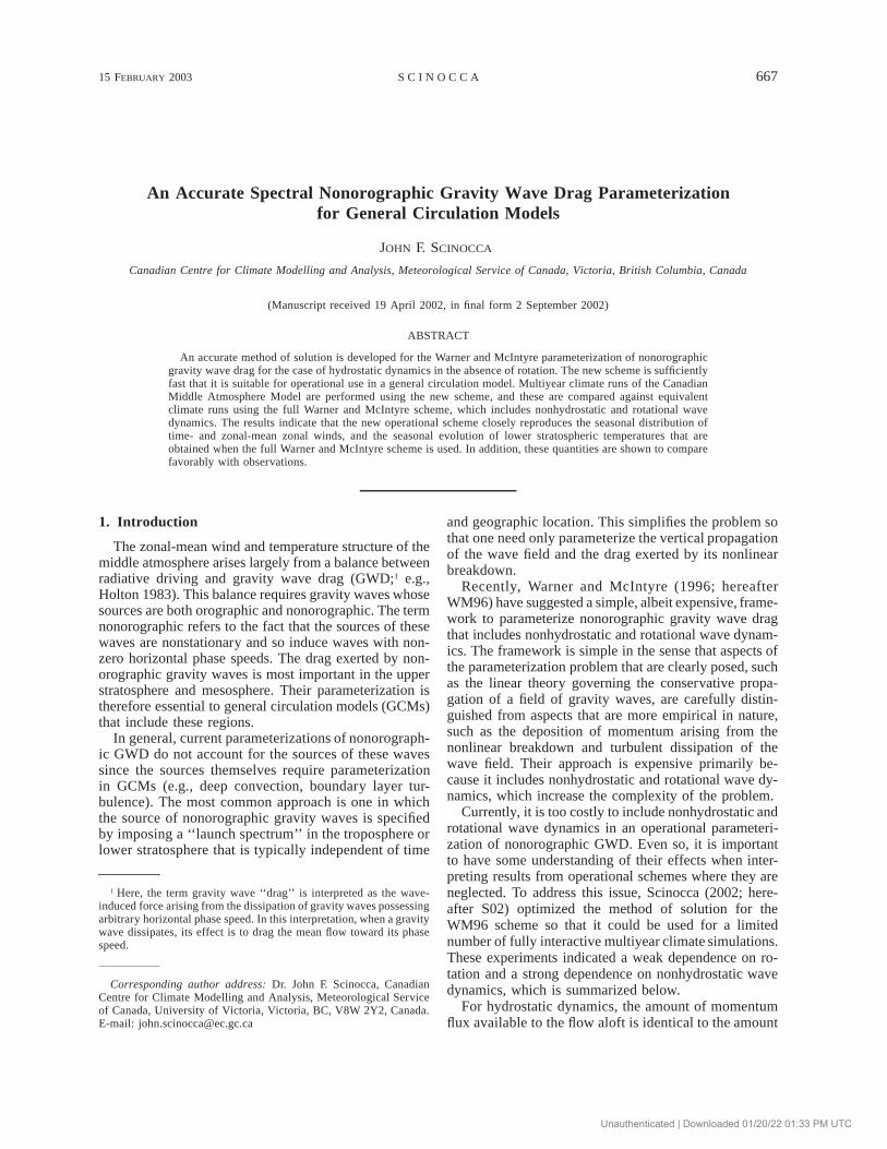
In Fig. 8 we present the time-mean zonal-mean zonalwinds for January and July from observations and fromthe two 5-yr climate runs. The observed winds, dis-played in Figs. 8a,b, are derived from the CooperativeInstitute for Research in the Atmosphere (CIRA) dataset(Fleming et al. 1990). Figs. 8c,d present the 5-yr av-eraged monthly mean winds from a run employing thefull N 1 R WM96 version of the nonorographic GWD

parameterization presented in S02. Figs. 8e,f present the5-yr averaged monthly mean winds from a run usingthe new operational scheme. The N 1 R simulationcompares favorably with the CIRA winds in both sea-sons. As discussed in S02, the use of the full WM96scheme in the CMAM alleviates a number of wind bi-ases that were present in the CMAM when the Hines(1997a,b) Doppler-spread nonorographic GWD param-eterization was used.

A comparison of the winds in Fig. 8 resulting fromthe application of the new operational scheme (Figs.8e,f) with the winds from the N 1 R run indicate aclose correspondence. By modifying the launch spec-trum for H 2 R dynamics in the new scheme, we havebeen able to alleviate much of the mesopause wind re-versal bias present in Fig. 6.

There remain a number of wind biases in Fig. 8. Forexample, there is the usual bias that the SH winter jetdoes not tilt as much as observed. This bias is presum-ably related to the fact that current gravity wave dragparameterizations are still too crude. Fluctuations ob-served in the lower tropical stratosphere of the N 1 Rrun (Figs. 8c,d) are related to quasi-biennial oscillations(QBO)-like oscillations, which are driven as a result ofthe greater launch momentum flux in this run. This isdiscussed at length in S02. The westerlies in the lowerstratosphere of the Northern Hemisphere during winterare too weak. This bias is also present on the tropo-spheric version of the model (e.g., see Scinocca andMcFarlane 2000) and appears to be unrelated to theparameterization of nonorographic gravity waves.

The new operational scheme is substantially moreefficient than the optimized N 1 R scheme developedin S02. Application of the N 1 R scheme in S02 was



FIG. 8. Time-mean zonal-mean zonal winds (m s21) for Jan and Jul (a), (b) CIRA data. Five–year run employing (c), (d) the N 1 Rversion of the WM96 scheme presented in S02, and (e), (f ) the new operational H 2 R version of WM96. Progressively darker shading hasbeen used to indicate regions of progressively increasing wind magnitude.

found to double the required computational (cpu) time.The new operational scheme employing the previousparameters (31) increases the cpu time of the GCM byapproximately 25%. This represents a factor of 4 sav-ings. Subsequent tests indicate that this cost can be re-duced to a 13% increase in cpu time with similar results(not shown). This additional savings may be achievedby reducing the number nc of horizontal phase speedsused to represent the E–P flux density in each azimuthfrom 35 to 15, reducing the maximum phase speed from2000 m s21 to 100 m s21, and, reducing G from 0.6 to0.25 (m s)21. For reference, the Hines Doppler-spread

parameterization (Hines 1997a,b) in the CMAM in-creases the cpu time by 18%.3

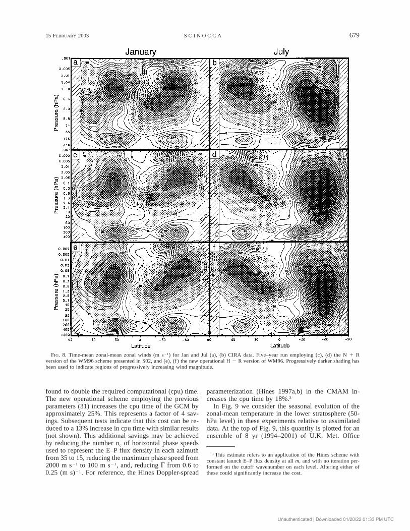
In Fig. 9 we consider the seasonal evolution of thezonal-mean temperature in the lower stratosphere (50-hPa level) in these experiments relative to assimilateddata. At the top of Fig. 9, this quantity is plotted for anensemble of 8 yr (1994–2001) of U.K. Met. Office

3 This estimate refers to an application of the Hines scheme withconstant launch E–P flux density at all m, and with no iteration per-formed on the cutoff wavenumber on each level. Altering either ofthese could significantly increase the cost.



FIG. 9. Ensemble seasonal evolution of zonal-mean temperature (K) near the 50-hPa level.(upper) Eight-year ensemble derived from UKMO operational assimilated data on the 46.4-hPa level. Five-year ensemble (middle) from the N 1 R S02 simulation, (lower) from thenew operational scheme.

(UKMO) operational assimilated data (Swinbank andO’Neill 1994). In Fig. 9a the middle and bottom, thisquantity is plotted for the full N 1 R S02 simulationand for the run using the new operational scheme, re-spectively. The two simulations display a close simi-larity to each other and compare favorably to the UKMO

assimilated data. The most obvious difference is a winterwarm pole bias in the simulations.

A number of factors could account for this bias. Thecold spring vortex seen in the UKMO data is aided byradiative cooling associated with the ozone loss due toheterogeneous chemical processes. These chemical pro-



cesses are not modeled in the simulations. Rather, ra-diative heating due to ozone is determined by a specifiedozone climatology. Here we have employ the middleatmosphere dataset of Kita and Sumi (1986). This olderclimatology does not contain an ozone hole and, there-fore, the associated cooling in the SH lower stratosphereduring late spring is not represented in the simulations.

The warm pole bias throughout the winter appears inpart due to a weakening of the polar vortex arising fromthe new orographic gravity wave drag parameterizationscheme (Scinocca and McFarlane 2000), which pro-duces more drag in the stratosphere than the orographicscheme used previously (McFarlane 1987). Sensitivitytests in which the strength of the orographic GWD isreduced (not shown) result in a stronger SH vortex andcolder, more realistic, temperatures throughout winter.The warm bias evident in the NH lower stratosphereduring winter is less sensitive to changes in the strengthof the orographic gravity wave drag. It similarly occursin a troposheric version of the model (Scinocca andMcFarlane 2000).

6. Summary

In this paper we have developed an operational ver-sion of the Warner and McIntyre (1996; WM96) spectralparameterization of nonorographic gravity wave dragfor hydrostatic dynamics in the absence of rotation (H2 R dynamics). Central to the derivation of the newoperational scheme is the simplification of the H 2 Rform of the E–P flux from rFH(m, , f) (used in S02)vto r (m, f) by integration over . This simplificationHF vreduces the required computational time by a factor of4 to 8. Here, we have demonstrated that, when the Dopp-ler shifting of is correctly accounted for in this in-vtegration, the use of r (m, f) is formally identical toHFthe use of rFH(m, , f) in the parameterization problem.v

This identity implies that all comparisons made be-tween the N 1 R scheme and the H 2 R scheme inS02 are equally valid for the the new operational schemeas well. In S02 it was found that simply reducing thetotal amount of E–P flux launched with H 2 R wavedynamics could crudely mimic the effects of back-re-flection obtained when nonhydrostatic and rotational (N1 R) wave dynamics were used in the scheme. In thisway, the H 2 R run of S02 was able to reproduce muchof the seasonal-mean zonal-mean zonal wind structureof the N 1 R run. The main bias appeared to be anunrealistically weak wind reversal at the summer me-sopause in the H 2 R run.

Here, using the new operational scheme, additionalmodifications to the launch spectrum were undertakento make the H 2 R system better compensate for theabsence of back-reflection. Five-year present-day cli-mate simulations employing the new operational schemerevealed that these modifications to the launch spectrumwere largely successful in eliminating this wind bias.Therefore, one of the main results of this analysis is

that the monthly mean zonal-mean winds and temper-atures obtained from use of the full N 1 R WM96scheme can be well reproduced by an H 2 R ‘‘opera-tional’’ scheme.

In addition, it was found that the seasonal evolutionof the zonal-mean temperature on the 50-hPa level wasvery similar between the full WM96 scheme (N 1 R)and the H 2 R operational scheme, and that both com-pared favorably with UKMO assimilated data. A modestwinter warm pole bias was identified in the simulations.This bias is thought in part to be associated with toomuch orographic gravity wave drag and the absence ofheterogeneous chemical processes in the simulations.

A portable version of the new operational schemederived here, and the N 1 R WM96 scheme presentedin S02 are freely available at http://www.cccma.bc.ec.gc.ca/;jscinocca/.

Acknowledgments. The author thanks Charles Mc-Landress, John Fyfe, and an anonymous reviewer fortheir careful reading of the manuscript and helpful com-ments.

REFERENCES

Abdella, K., and N. A. McFarlane, 1996: Parameterization of thesurface-layer exchange coefficients for atmospheric models.Bound.-Layer Meteor., 80, 223–248.

Beagley, S. R., J. de Grandpre, J. N. Koshyk, N. A. McFarlane, andT. G. Shepherd, 1997: Radiative–dynamical climatology of thefirst-generation Canadian middle atmosphere model. Atmos.–Ocean, 35, 293–331.

Fleming, E. L., S. Chandra, J. J. Barnett, and M. Corney, 1990: Zonalmean temperature, pressure, zonal wind and geopotential heightas functions of latitude. Adv. Space Res., 10, 11–59.

Fritts, D. C., and T. E. VanZandt, 1993: Spectral estimates of gravitywave energy and momentum fluxes. Part I: Energy dissipation,acceleration, and constraints. J. Atmos. Sci., 50, 3685–3694.

Gill, A. E., 1982: Atmosphere–Ocean Dynamics. Academic Press,662 pp.

Hines, C. O., 1997a: Doppler-spread parameterization of gravity-wave momentum deposition in the middle atmosphere. Part I:Basic formulation. J. Atmos. and Solar-Terr. Phys., 59, 371–386.

——, 1997b: Doppler-spread parameterization of gravity-wave mo-mentum deposition in the middle atmosphere. Part II: Broad andquasi monochromatic spectra, and implementation. J. Atmos. andSolar-Terr. Phys., 59, 387–400.

Holton, J. R., 1983: The influence of gravity wave breaking on thegeneral circulation of the middle atmosphere. J. Atmos. Sci., 40,2497–2507.

Holzer, M., 1996: Optimal spectral topography and its effect on modelclimate. J. Climate, 9, 2443–2463.

Kita, K., and A. Sumi, 1986: Reference ozone models for middleatmosphere. Meteorological Research Rep. 86-2, Division ofMeteorology, Geophysical Institute, University of Tokyo, 26 pp.

McFarlane, N. A., 1987: The effect of orographically excited gravitywave drag on the circulation of the lower stratosphere and tro-posphere. J. Atmos. Sci., 44, 1175–1800.

——, G. J. Boer, J. P. Blanchet, and M. Lazare, 1992: The CanadianClimate Centre second-generation general circulation model andits equilibrium climate. J. Climate, 5, 1013–1044.

Scinocca, J. F., 2002: The effect of back-reflection in the parametri-zation of non-orographic gravity-wave drag. .J. Meteorol. Soc.Japan, 80, 939–962.



——, and N. A. McFarlane, 2000: The parameterization of drag in-duced by stratified flow over anisotropic orography. Quart. J.Roy. Meteor. Soc., 126, 2353–2393.

Swinbank, R., and A. O’Neill, 1994: A stratosphere–troposphere dataassimilation system. Mon. Wea. Rev., 122, 686–702.

Verseghy, D. L., N. A. McFarlane, and M. Lazare, 1993: A Canadianland surface scheme for GCMs: II. Vegetation model and coupledruns. Int. J. Climatol., 13, 347–370.

Warner, C. D., and M. E. McIntyre, 1996: On the propagation and

dissipation of gravity wave spectra through a realistic middleatmosphere. J. Atmos. Sci., 53, 3213–3235.

——, and ——, 1999: Toward an ultra-simple spectral gravity waveparameterization for general circulation models. Earth PlanetsSpace, 51, 475–484.

——, and ——, 2001: An ultrasimple spectral parameterization fornonorographic gravity waves. J. Atmos. Sci., 58, 1837–1857.

Zhang, G. J., and N. A. McFarlane, 1995: Sensitivity of climatesimulations to the parameterization of cumulus convection in theCCC-GCM. Atmos.–Ocean, 3, 407–446.


Documents

An Accurate Spectral Nonorographic Gravity Wave Drag