Embed Size (px)
Citation preview

American-StyleDerivatives
Valuation and Computation
CHAPMAN & HALL/CRC FINANCIAL MATHEMATICS SERIES
© 2006 by Taylor & Francis Group, LLC

CHAPMAN & HALL/CRCFinancial Mathematics Series
Aims and scope:The field of financial mathematics forms an ever-expanding slice of the financialsector. This series aims to capture new developments and summarize what is knownover the whole spectrum of this field. It will include a broad range of textbooks,reference works and handbooks that are meant to appeal to both academics andpractitioners. The inclusion of numerical code and concrete real-world examples ishighly encouraged.
Series EditorsM.A.H.DempsterCentre for Financial ResearchJudge Institute of ManagementUniversity of Cambridge
Dilip B.MadanRobert H.Smith School of BusinessUniversity of Maryland
Rama ContCMAPEcole PolytechniquePalaiseau, France
Proposals for the series should be submitted to one of the series editors above or directly to:CRC Press, Taylor and Francis Group24–25 Blades CourtDeodar RoadLondon SW15 2NUUK
© 2006 by Taylor & Francis Group, LLC

CHAPMAN & HALL/CRC FINANCIAL MATHEMATICS SERIES
American-StyleDerivatives
Valuation and Computation
Jérôme Detemple
Boca Raton London New York
© 2006 by Taylor & Francis Group, LLC

Published in 2006 byChapman & Hall/CRCTaylor & Francis Group6000 Broken Sound Parkway NW, Suite 300Boca Raton, FL 33487–2742
© 2006 by Taylor & Francis Group, LLCChapman & Hall/CRC is an imprint of Taylor & Francis Group
No Claim to original U.S. Government WorksPrinted in the United States of America on acid-free paper10 9 8 7 6 5 4 3 2 1
International Standard Book Number-10:1-58488-567-X (Hardcover)International Standard Book Number-13:978-1-58488-567-2 (Hardcover)Library of Congress Card Number 2005052861
This book contains information obtained from authentic and highly regarded sources. Reprintedmaterial is quoted with permission, and sources are indicated. A wide variety of references are listed.Reasonable efforts have been made to publish reliable data and information, but the author and thepublisher cannot assume responsibility for the validity of all materials or for the consequences oftheir use.
No part of this book may be reprinted, reproduced, transmitted, or utilized in any form by anyelectronic, mechanical, or other means, now known or hereafter invented, including photocopying,microfilming, and recording, or in any information storage or retrieval system, without writtenpermission from the publishers.
For permission to photocopy or use material electronically from this work, please accesswww.copyright.com (http://www.copyright.com/) or contact the Copyright Clearance Center, Inc.(CCC) 222 Rosewood Drive, Danvers, MA 01923, 978–750–8400. CCC is a not-for-profitorganization that provides licenses and registration for a variety of users. For organizations thathave been granted a photocopy license by the CCC, a separate system of payment has beenarranged.
Trademark Notice: Product or corporate names may be trademarks or registered trademarks, andare used only for identification and explanation without intent to infringe.
Library of Congress Cataloging-in-Publication Data
Detemple, Jérôme.American-style derivatives : valuation and computation / Jerome Detemple.
p. cm.—(Chapman & Hall/CRC financial mathematics series)Includes bibliographical references and index.ISBN 1–58488–567–X (alk. paper)1. Derivative securities—United States. 2. Derivative securities—Valuation. I. Title. II.Series.
HG6024.U6D49 2005332.64’57—dc22 2005052861
Visit the Taylor & Francis Web site athttp://www.taylorandfrancis.com
and the CRC Press Web site athttp://www.crcpress.com
© 2006 by Taylor & Francis Group, LLC

DedicationTo Pamela, Michael and Alfie, for their love and support.
© 2006 by Taylor & Francis Group, LLC

AcknowledgmentsI benefitted from the comments of several generations of students at MIT,McGill and Boston University to whom I taught material included in thisbook. The remarks of Weidong Tian, Zhiguo He and Jing Zhou were especiallyappreciated. Special thanks are due to Mark Broadie. Much of this book isbased on joint work that we undertook during the past decade. I have benefittedfrom our discussions on various aspects associated with the valuation ofderivatives. Most of all I am indebted to him for introducing me to some ofthe subtleties arising in the computation of derivative securities’ prices.Thanks are also due to Ioannis Karatzas, who taught me a great deal aboutstochastic processes and their application to financial models. His insightsand contributions have shaped my own thinking and permeate severalchapters of this book. Finally, I bear an obvious intellectual debt to the foundingfathers and early pioneers of the field: Fisher Black, Myron Scholes, BobMerton, Steve Ross and John Cox.
© 2006 by Taylor & Francis Group, LLC

BiographyJérôme Detemple is Professor of Finance and Economics at Boston UniversitySchool of Management and an Associate Fellow at CIRANO. He holds a Ph.D.in Finance from the Wharton School, University of Pennsylvania, and aDoctorat D’État ès Sciences Économiques from Université Louis Pasteur inStrasbourg. His scholarly work is primarily in the fields of mathematicalfinance and financial economics. He is the author of 40 articles in leadingacademic journals and is widely known for his contributions to derivativesecurities valuation, risk management and asset allocation. ProfessorDetemple is currently on the editorial boards of Mathematical Finance,Management Science and the Review of Derivatives Research. He is a pastassociate editor of the Review of Financial Studies.
© 2006 by Taylor & Francis Group, LLC

1 Introduction 1
2 European Contingent Claims 72.1 Definitions 72.2 The Economy 82.3 Attainable Contingent Claims 102.4 Valuation of Attainable Claims 142.5 Claims Involving Negative Payoffs 162.6 The Structure of Contingent Claims’ Prices 182.7 Changes of Numeraire and Valuation 192.8 Option and Forward Contracts 212.9 Markets with Deterministic Coefficients 242.10 Markets with Multiple Assets 282.11 Appendix: Proofs 29
3 American Contingent Claims 373.1 Contingent Claims with Random Maturity 373.2 American Contingent Claims 393.3 Exercise Premium Representations 413.4 A Duality Formula: Upper Price Bounds 443.5 American Options and Forward Contracts 453.6 Multiple Underlying Assets 473.7 Appendix: Proofs 48
4 Standard American Options 554.1 The Immediate Exercise Region 554.2 The Call Price Function 574.3 Early Exercise Premium Representation 594.4 A One-Dimensional Integral Equation 614.5 Hedging 624.6 Diffusion Processes 634.7 Floating Strike Asian Options 674.8 American Forward Contracts 694.9 Appendix: Proofs 71
Contents
© 2006 by Taylor & Francis Group, LLC

CONTENTS
5 Barrier and Capped Options 855.1 Barrier Options 85
5.1.1 Definitions and Literature 855.1.2 Valuation 86
5.2 Capped Options 895.2.1 Definitions, Examples and Literature 895.2.2 Constant Cap 895.2.3 Capped Options with Growing Caps 935.2.4 Stochastic Cap, Interest Rate and Volatility 96
5.3 Diffusion Processes 975.4 Appendix: Proofs 98
6 Options on Multiple Assets 1076.1 Definitions, Examples and Literature 1076.2 The Financial Market 1096.3 Call Options on the Maximum of 2 Prices 109
6.3.1 Exercise Region of a Max-Call Option 1106.3.2 Valuation of Max-Call Options 1146.3.3 Dual Strike Max-Options 1196.3.4 Put Options on the Minimum of 2 Prices 1206.3.5 Economic Implications 120
6.4 American Spread Options 1216.4.1 Exercise Region and Valuation 1216.4.2 Options to Exchange One Asset for Another 1236.4.3 Exchange Options with Proportional Caps 124
6.5 Options on an Average of 2 Prices 1256.5.1 Geometric Averaging 1256.5.2 Arithmetic Averaging 126
6.6 Call Options on the Minimum of 2 Prices 1296.6.1 Exercise Region of a Min-Call Option 1296.6.2 The EEP Representation 1326.6.3 Integral Equations for the Boundary Components 135
6.7 Appendix A: Derivatives on Multiple Assets 1356.8 Appendix B: Proofs 143
7 Occupation Time Derivatives 1557.1 Background and Literature 1557.2 Definitions 1567.3 Symmetry Properties 1577.4 Quantile Options 158
7.4.1 Contractual Specification 1587.4.2 The Distribution of an α-Quantile 1597.4.3 Pricing Quantile Options 1597.4.4 A Reduction in Dimensionality 1627.4.5 Quantile Contingent Claims 163
7.5 Parisian Options 163
© 2006 by Taylor & Francis Group, LLC

CONTENTS
7.5.1 Contractual Specification 1647.5.2 Parity and Symmetry Relations 1657.5.3 Pricing Parisian Options 1667.5.4 Parisian Contingent Claims 169
7.6 Cumulative Parisian Contingent Claims 1707.6.1 Definitions and Parity/Symmetry Relations 1707.6.2 Pricing Cumulative Barrier Claims 1717.6.3 Standard and Exotic Cumulative Barrier Options 172
7.7 Step Options 1737.7.1 Contractual Specification 1737.7.2 Pricing European-style Step Options 174
7.8 American Occupation Time Derivatives 1757.8.1 Early Exercise Premium Representation 1757.8.2 Valuation in the Standard Model 176
7.9 Multiasset Claims 1797.9.1 Symmetry Properties 1797.9.2 Valuation 181
7.10 Appendix: Proofs 181
8 Numerical Methods 1958.1 Numerical Methods for American Options 1958.2 Integral Equation Methods 1978.3 Exercise Time Approximations: LBA-LUBA 199
8.3.1 A Lower Bound for the Option Price 1998.3.2 A Lower Bound for the Exercise Boundary 2008.3.3 An Upper Bound for the Option Price 2018.3.4 Price Approximations 202
8.4 Diffusion Processes 2028.4.1 Integral Equation Methods 2038.4.2 Stopping Time Approximations: LBA and LUBA 203
8.5 Other Recent Approaches 2048.5.1 Lattice Methods: Binomial Black-Scholes Algorithm 2048.5.2 Integral Equation: Non-linear Approximations 2048.5.3 Monte Carlo Simulation 205
8.6 Performance Evaluation 2058.6.1 Experiment Design 2068.6.2 Results and Discussion 206
8.7 Methods for Multiasset Options 2078.7.1 Lattice Methods 2078.7.2 Monte Carlo Simulation 2098.7.3 Monte Carlo Simulation and Duality 211
8.8 Methods for Occupation Time Derivatives 2128.8.1 Laplace Transforms 2128.8.2 PDE-based Methods 2128.8.3 Binomial/Trinomial Lattices 213
8.9 Appendix: Proofs 215
© 2006 by Taylor & Francis Group, LLC

CONTENTS
Bibliography 217
© 2006 by Taylor & Francis Group, LLC

1
Chapter 1
Introduction
Derivative securities have become common financial instruments thatappear in multiple areas of economic activity. Contracts of this type havebeen exchanged for several centuries among economic agents. But it isonly during the past three decades, since the creation of the first organizedoptions market, the Chicago Board of Options Exchange (CBOE), that thederivatives industry has experienced rapid growth. Since the opening ofthis market, the number and types of contracts have substantiallyincreased. Today’s investor can trade foreign exchange options, futurescontracts, index options, bond options, energy derivatives and weatherderivatives in organized markets. Additionally, advances in pricing theoryand in technology during the past ten years have made it possible toengineer contracts with new provisions designed to meet all kinds of specificinvestment or financing needs. Capped options, Asian options, shout optionsand other types of exotic securities can now be purchased in the over-the-counter market or are issued by firms with particular objectives in mind.Option-like payoffs also permeate the activities of firms and the rewardstructures granted to managers and employees. Economic agents arebecoming increasingly aware of the benefits and pitfalls associated withthe use of derivative products.
This book provides an extensive treatment of theoretical andcomputational aspects of derivative securities pricing, with a particularemphasis on the valuation of American-style derivatives. The cross-disciplinary nature of this topic has been the trigger for a multitude ofcontributions dealing with various aspects of the valuation process.Inevitably, a selection of themes had to be made. Every effort has beenmade to present the most important aspects of the field. Part of thisselection, nevertheless, reflects my own perceptions as well as personalresearch interests. Effort has also been made to provide appropriatereferences to the literature dealing with the results presented. Apologiesare extended to those whose contributions may have been inadvertentlyoverlooked.
The remainder of this introduction provides perspective on the variousthemes addressed. Important milestones in the development of a pricing
© 2006 by Taylor & Francis Group, LLC

2 CHAPTER 1. INTRODUCTION
theory for American-style contracts are surveyed. Part of this overviewparallels the order in which the various topics are dealt with in thesubsequent chapters. In certain places, however, chronological order takesprecedence, in order to provide a better understanding of the evolution ofthe field.
The valuation of derivative securities has been the object of a long quest.A model describing the random behavior of speculative asset prices wasproposed very early on, by Bachelier [1900]. The development of a rigoroustheory of option pricing, however, only dates back to the 1970s, with theseminal papers of Black and Scholes [1973] and Merton [1973a]. The majorcontribution of this work can be viewed as a valuation approach consistentwith the absence of arbitrage opportunities in the financial market. Blackand Scholes used this methodology to price European options and relatedcontingent claims in a simple model, where the underlying price follows ageometric Brownian motion and the interest rate is constant (the standardmarket model). Merton refined and extended the approach to more generalsettings. An equivalent methodology, based on an appropriately chosen“risk-neutral” valuation operator, was pioneered, a few years later, by Coxand Ross [1976]. The foundations and principles underlying this valuationmethod were identified and characterized in the fundamental papers ofHarrison and Kreps [1979] and Harrison and Pliska [1981].
The valuation of American options also has a long history. Samuelson[1965] and McKean [1965] were the first to treat this problem as a stoppingtime problem involving the option’s payoff and the underlying pricedistribution. McKean, furthermore, showed that the stopping problem couldbe converted into a free boundary problem. It is only more recently, however,that the optimal stopping problem has been posed relative to an appropriatemeasure, the Cox-Ross risk neutral measure, that correctly prices Americanoptions (Bensoussan [1984] and Karatzas [1988]). Karatzas [1988], inparticular, shows that the American option payoff can be replicated by acarefully chosen policy of investment in the primary assets in the model.The value of the American option must then be equal to the value of thereplicating portfolio in order to avoid arbitrage opportunities and beconsistent with equilibrium in the capital market.
While the stopping time approach to American option valuation isinstructive, it does not provide immediate insights into the properties ofthe optimal exercise boundary, nor does it lead to efficient numericalprocedures. Nevertheless, building on this approach, Kim [1990], Jacka[1991] and Carr, Jarrow and Myneni [1992] were able to derive, in thecontext of the standard market model, a useful decomposition of theAmerican option value, that emphasizes the premium attached to earlyexercise, i.e., exercise before the maturity date. This early exercise premium(EEP) representation expresses the value of the American option as thecorresponding European option value plus the gain from early exercise.The gain from early exercise is the present value of the dividend benefits
© 2006 by Taylor & Francis Group, LLC

3
in the exercise region net of the interest losses on the payments incurredupon exercise.
In fact, the EEP formula ties back to the general theory of stochasticprocesses and more specifically to the Riesz decomposition of asupermartingale. This connection materializes because the option valuationproblem, which is a stopping time problem involving a particular payofffunction, is solved by taking the smallest supermartingale majorant of thepayoff. This particular supermartingale is called the Snell envelope of thepayoff function. The Riesz decomposition breaks the Snell envelope downinto two parts, a martingale and a potential, and the latter corresponds tothe EEP component of the option value. The Riesz decomposition of thevalue function associated with a stopping time problem was establishedby El Karoui and Karatzas [1991]. Their result was subsequently appliedby Myneni [1992], to price an American put in the standard market model.The decomposition has since been extended, by Rutkowski [1994], to amore general class of market models with semimartingale prices.
The early exercise premium representation has a parametric flavor asit expresses the American option value in terms of the unknown optimalexercise boundary. But, by using the fact that immediate exercise is optimalwhen the asset price reaches the boundary, the EEP formula also producesa recursive integral equation for the optimal exercise boundary. Thisintegral equation is useful for several purposes. For one it can serve as astarting point for a study of the exercise boundary and its properties. Itcan also be used for computational purposes. To calculate the Americanoption value it suffices to solve the integral equation for the boundary andthen to substitute this solution back in the EEP formula. In recent yearssubstantial research efforts have been devoted to this two-stage procedure.Several computational schemes have been proposed and variousmodifications of the integral equation, designed to simplify calculations,have been developed.
While the valuation of standard American option contracts has nowachieved a fair degree of maturity, much work remains to be done regardingthe new contractual forms that are constantly emerging in response toevolving economic conditions and regulations. Innovations that havereceived attention include barrier options and capped options. Both typesof contracts contain provisions designed to limit the payoffs under certainconditions. Barrier options, typically, condition the payoffs on the occurrenceof events involving first passage times. For instance, a knock-out barrieroption automatically expires if the underlying asset price reaches aprespecified threshold. A knock-in barrier option, on the contrary, comesinto existence if such an event materializes. Capped options have a ceilingon their payoff that limits the potential gains from early exercise. Barrierand capped options are attractive from the perspective of issuers becausethey limit potential liabilities. Yet, they also remain attractive forpurchasers as they retain an upside potential and are less costly than
© 2006 by Taylor & Francis Group, LLC

4 CHAPTER 1. INTRODUCTION
their plain vanilla counterparts. As a result, payoffs of this sort haveappeared as components of securities issued by firms to cover certainfinancing needs. The valuation of these instruments can be quite involveddepending on the exact nature of the contractual provisions. Thoroughtreatments of American-style versions of these contracts, in the standardmarket model, can be found in Broadie and Detemple [1995] and Gao,Huang and Subrahmanyam [2000]. Valuation formulas and principles forcapped options also prove useful for the valuation of American-style vanillaoptions. Properly designed capped options, indeed, can provide accurateapproximations of standard American option prices.
Our understanding of contracts written on multiple underlying assetsis also limited, in comparison to the single asset case. Recent papers havemade progress on that front, identifying the structure of immediate exerciseregions associated with a variety of multiasset derivatives such as max-options, min-options and spread options (Tan and Vetzal [1994], Riddiough,Geltner and Stojanovic [1996], Gerber and Shiu [1997], Broadie andDetemple [1997a], Villeneuve [1997], Detemple, Feng and Tian [2003]).Some of the surprising properties documented in this literature show thatoptimal exercise decisions are not simple extrapolations of those prevailingin the single asset case. Proper identification of these policies becomescritical, in some cases, for capturing the full benefits associated with theearly exercise provision.
Occupation time derivatives are among the latest innovations to appearin derivatives markets. Contracts of this sort have the common propertyof depending on the time spent by the underlying asset price in certainregions of the state space. Simple examples are payoffs depending on theamount of time above (or below) a fixed barrier. An option that comes intoexistence when the underlying price spends more than a prespecifiedamount of time below a given barrier is a more specific illustration. Thiscontract, called a cumulative knock-in barrier option, is a naturalgeneralization of the standard (one-touch) knock-in option that comes intoexistence at the first touch of the barrier. A variety of contracts withprovisions based on occupation times have been examined. Quantileoptions, Parisian options and step options are perhaps the better knownexamples. European-style contracts of these types have been thoroughlystudied and pricing formulas have been derived. Fundamentalcontributions in the area include Akahori [1995], Dassios [1995], Chesney,Jeanblanc-Picque and Yor [1997], Hugonnier [1999] and Linetsky [1999].Little attention has been devoted to American-style versions of these claims:some results are provided herein.
Computational aspects of derivatives valuation have also been the subjectof much research. The set of numerical techniques available for valuingAmerican options is now vast and has increased substantially since the earlydevelopments of the 70s. Major approaches include the binomial methodinitiated by Cox, Ross and Rubinstein [1979], techniques based on partial
© 2006 by Taylor & Francis Group, LLC
5
differential equations developed by Schwarz [1977] and Brennan andSchwarz [1977], [1978], methods based on the integral equation of Kim[1990], Jacka [1991] and Carr, Jarrow and Myneni [1992], variationalinequalities techniques proposed by Jaillet, Lamberton and Lapeyre [1990]and Monte Carlo simulation methods initiated by Boyle [1977]. A numberof new approaches or modifications of existing methods have been proposedrecently. Recent techniques based on approximations of stopping times(Broadie and Detemple [1996]), of partial differential equations (Carr andFaguet [1995]) or of integral equations (Ju [1998]) yield substantialimprovements over traditional approaches. Modifications of the binomialmethod such as BBS (Binomial with Black-Scholes modification) also exhibitimproved performance. An extensive study comparing the performances ofvarious methods available appears in Broadie and Detemple [1996]. Thenew developments, that have taken place since that study, concern mainlythe numerical valuation of American multiasset derivatives. But even thoughseveral computational approaches have been proposed to handle thesecomplex securities (Broadie and Glasserman [1997a], [1997b], Rogers [2002],Haugh and Kogan [2003], Andersen and Broadie [2004]), their efficientnumerical evaluation still remains a challenge.
The layout of the book is as follows. The second chapter reviews valuationprinciples for European contingent claims in a financial market in whichthe underlying asset price follows an Ito process and the interest rate is
In this context the basic valuation principles for American options are laidout. Two instructive representation formulas, the EEP decomposition andthe delayed exercise premium (DEP) decomposition, are also described.
Black-Scholes market setting (i.e., the model with constant coefficients). Areduction of the integral equation as well as studies of related contractualforms are also presented in this context. American barrier and capped
are first provided in the standard model with dividend-paying assets.Results are also presented for non-dividend-paying assets when theunderlying asset price follows an Itô process with stochastic volatility and
options written on multiple underlying assets. Immediate exercise regionsare identified and valuation formulas provided, for a variety of popular
occupation time derivatives. Standard contractual forms are described andanalyzed. Valuation formulas are reported for European-style and some
is on the computation of American-style options and emphasis is placed onrecent developments. An efficiency study is carried out to evaluate theperformance of some of these methods. All proofs are collected in appendices,found at the end of each chapter.
© 2006 by Taylor & Francis Group, LLC
These results are applied in chapter 4 to American option valuation in the
options are analyzed in chapter 5. For capped options, valuation formulas
the cap’s growth rate is an adapted stochastic process. Chapter 6 examines
multiasset option contracts. Chapter 7 provides an introduction to
American-style claims. Chapter 8 is devoted to numerical methods. Focus
stochastic. Chapter 3 extends the analysis to American contingent claims.
7
Chapter 2
European Contingent Claims
This chapter deals with the valuation of European-style financial claims. Wefirst define the class of contingent claims that is the focus of our analysis(section 2.1) and describe the financial market setting (section 2.2). Wethen value European contingent claims (sections 2.3–2.7), examine optionand forward contracts (section 2.8) and specialize the results to marketswith deterministic coefficients (section 2.9). Lastly, we outline an extensionto a market with multiple assets (section 2.10).
2.1 DefinitionsBroadly speaking a contingent claim is a financial contract whose payoff iscontingent on the state of nature. In its most general form a contingent claimgenerates a flow of payments over periods of time as well as cash paymentsat specific dates. The cash flows involved need not be paid at fixed points intime or during fixed periods of time. Some claims involve payments atprespecified random times or even at (random) times that are chosen by theholder of the contract. A contingent claim is said to be European-style if thetiming of the contractual payments is specified at the outset. It is American-style if the timing of the payments is chosen by the owner of the claim.
Derivative securities are examples of contingent claims. They aretypically defined as financial contracts whose payoffs depend on the price(s)of some underlying or primary asset(s). In this case the state dependencein the payoff of the contract arises through the market price(s) of someother asset(s).
The standard example of a derivative security is an option contract. Anoption gives the holder of the contract the right, but not the obligation, tobuy (or sell) a given asset, at a predetermined price (the exercise or strikeprice), at or before some prespecified future date (the maturity date). Theoption to buy (sell) is a call (put) option. A European-style option contractcan only be exercised at the fixed maturity date T. At that time, exercise isoptimal if and only if the option produces a non-negative cash flow; in thatevent the option is said to be in the money. The payoff of a European calloption is therefore (ST - K)+ ≡ max (ST - K, 0), where ST is the underlying
© 2006 by Taylor & Francis Group, LLC

8 CHAPTER 2. EUROPEAN CONTINGENT CLAIMS
asset price at the specified maturity date and K > 0 is the exercise price of thecontract. The payoff of a European put option is (K - ST)+. American-styleoptions, which can be exercised as desired, at or before the maturity date,have similar payoff functions upon exercise.
2.2 The EconomyThe economy has the following characteristics. Uncertainty is representedby a complete probability space (�, F, P) where � is the set of elementaryevents or “states of nature” with generic element �, F is a �-algebrarepresenting the collection of observable events and P is a probabilitymeasure defined on (�, F). The time period is the finite interval [0, T]. Astandard Brownian motion process z is defined on (�, F, P) with values inR. The flow of information is given by the natural filtration F(.), i.e., the P-augmentation of the filtration generated by the Brownian motion. Thus,information at any time t consists in the observed trajectory of the Brownianmotion process up to time t. Without loss of generality we set FT = F so thatall the observable events are eventually known. Our model for informationand beliefs is (�, F, F(.), P).
Two types of investment opportunities, riskless and risky, are available inthe asset market. The riskless asset (the bond) can be interpreted as a bankaccount, bearing interest at the locally riskless rate r. An investment in thisaccount equal to B0, at time t = 0, evolves according to
(2.1)
The interest rate r is a stochastic process that is bounded, strictly positiveand progressively measurable.1 For later use, define the discount factor
The risky asset (the stock) has a price
S satisfying the stochastic differential equation
(2.2)
The process � represents the dividend yield on the stock; μ and � are,respectively, the drift and the volatility coefficients of the stock’s total rateof return (the return from capital gains plus the dividend yield: dS/S +�dt). The coefficients �, μ, and � are bounded and progressively measurableprocesses of the filtration. The dividend rate is non-negative, � � 0; thevolatility � is bounded above and bounded away from zero (P-a.s.). Theprice that solves (2.2) is the ex-dividend stock price. The gains process G iscomposed of capital gains and dividends (dG = dS + S�dt). The (total) rateof return is the gains process divided by the price (dS/S + �dt = dG/S).
1Given the uncertainty setting adopted here, a process X is said to be progressivelymeasurable if it depends on the trajectories of the Brownian motion z and on time.Formally, X is progressively measurable if Xt is Ft × B([0, t]) measurable for all t ∈ [0, T],where B([0, t]) denotes the Borel sigma-field on [0, t].
© 2006 by Taylor & Francis Group, LLC

9
The assumption that the return volatility be bounded away from zeroensures that an investor can always trade in the Brownian motion bytrading the stock. As a result any financial exposure that is affected by therandom fluctuations in the Brownian motion can be hedged. When this isthe case the financial market is said to be complete.
Remark 1 Alternative definitions of market completeness can beformulated. A natural one is to say that the financial market is completewhen any state contingent claim with an F(.)-progressively measurablepayoff process (i.e., cash flows that depend on the realized trajectories ofthe Brownian motion process z) can be manufactured by selecting anappropriate portfolio of traded financial assets and investing a suitableinitial amount. Modulo some technical conditions on the class of claimsinvolved, this definition is equivalent to the one above. When the volatilitycoefficient σ is bounded away from zero, the stochastic shocks affecting thefinancial market (the Brownian motion z) can be hedged, at all times, byinvesting in the stock. The ability to pursue unconstrained investmentpolicies in the stock and in the locally riskfree asset, then, ensures theattainability of these contingent claims (Karatzas and Shreve [1998,Section 1.6]. See also Harrison and Kreps [1979], Harrison and Pliska[1981], Duffie [1986]). A formalization of some of these ideas is provided inthe next section.
It has become standard practice to use stochastic processes of the form(2.2) to model the behavior of stock prices. For instance the geometricBrownian motion process, obtained by taking constant coefficients (μ,�,δ), isused as a basis for the Black and Scholes [1973] analysis. Typical Markovianmodels with price-dependent volatility, interest rate or dividend rate can alsobe embedded in this structure (see section 4.6 in chapter 4). The specificationin (2.2) is more general to the extent that it allows for general dependenciesbetween the coefficients and the trajectories of the underlying Brownianmotion.2
In order to determine the prices of contingent claims one needs tocharacterize the set of random variables (payoffs) that can be manufactured(replicated) by trading the assets available, namely the stock and the bond.To this end a description of the stochastic process representing the valueof an account associated with a portfolio policy is needed. Let X be thevalue of this account, i.e., the wealth process associated with an investmentpolicy in the financial assets (2.1)–(2.2). We first define the notions ofconsumption (i.e., withdrawal) and portfolio policies, and the set of “feasible”or “admissible” consumption-portfolio policies.
A portfolio policy π is a progressively measurable, R-valued stochasticprocess such that . Here πt denotes the (dollar)
2 Alternative formulations that have received attention include processes with jumps (Merton[1973a], Cox and Ross [1976]).
2.2. THE ECONOMY
© 2006 by Taylor & Francis Group, LLC

10 CHAPTER 2. EUROPEAN CONTINGENT CLAIMS
investment in the stock at date t; the amount invested in the riskless asset isXt - �t. A cumulative consumption policy C is a progressively measurable,non-decreasing, right-continuous process with values in R, initial value C0 =0 and CT < � (P - a.s.). Consumption amounts to a withdrawal of funds fromthe account; injections are not permitted at this stage. When cumulativeconsumption is null at all times the portfolio is said to be self-financing: itinvolves neither infusions nor withdrawals of funds but only rebalancing ofthe positions held in the different assets.
An investment amounting to �t in the stock at date t produces a gain(capital gains plus dividends) equal to . An investmentof Xt - �t in the bond gives a gain of (Xt - �t)rtdt. The activity of consumptionreduces wealth by the corresponding amount dCt. A consumption-portfoliopolicy (C, �) therefore leads to a wealth process X that is described by thestochastic differential equation
(2.3)
where x denotes the initial amount invested. Given an initial investment x> 0, a consumption-portfolio policy (C, �) is admissible, if the associatedwealth process X solving (2.3) satisfies the non-negativity constraint
(2.4)
This condition is a no-bankruptcy condition mandating that wealth cannotbe negative during the trading period. Non-negativity of wealth does notpreclude policies that involve short sales of the stock (� < 0) or borrowingat the riskfree rate (X - � < 0). Let A(x) be the set of admissible policies.
A European-style contingent claim (f, Y) is composed of a cumulativepayment process f and a terminal cash flow Y at date T. The cumulativepayment process is a finite variation process that is non-decreasing,progressively measurable, right-continuous and null at zero. The terminalcash flow is a non-negative FT-measurable random variable. A consumption-portfolio policy (C, �) replicates a European contingent claim (f, Y) at initialcost x if (C, �) is admissible, dCt = dft, and XT = Y. We also say that (C, �)generates the claim (f, Y). The claim (f, Y) is attainable from an initialinvestment x if there exists an admissible consumption-portfolio policysuch that dCt � dft for all t ∈ [0, T] and XT � Y (P-a.s.). Such a consumption-portfolio policy is said to attain or super-replicate (f, Y) from x.
2.3 Attainable Contingent ClaimsThe pricing of contingent claims amounts to the identification of anappropriate valuation operator that maps future payoffs into current prices.Given that the processes satisfying (2.1) and (2.2) represent the values of
© 2006 by Taylor & Francis Group, LLC
11
traded assets, the valuation operator must be consistent with these existingprices. In fact, as will become clear below, the price processes (2.1) and(2.2) completely determine the valuation operator in our economic setting.
The market model (2.1)–(2.2) implies a unique market price of risk (MPR) defined as . This one-dimensional process isprogressively measurable and bounded, because � is bounded away fromzero. It is also uniquely defined. This is a typical implication of the abilityto trade, at all times, in the underlying source of uncertainty, the Brownianmotion. That is, it is a direct implication of market completeness. Themarket price of risk represents the expected excess return (over the riskfreerate) implicitly assigned by the model (2.1)–(2.2) to the stochastic shocks zaffecting the financial market. It is also known as the Sharpe ratio.
Consider now the exponential process η defined by
(2.5)
This process is progressively measurable and positive. An application of Ito’slemma shows that is a local martingale .3 Given that anynon-negative local martingale is a supermartingale we see that the process is actually a supermartingale (see Karatzas and Shreve [1988, Chapter1, Problem 5.19]).4 Moreover, boundedness of the market price of risk impliesthat the Novikov condition is satisfied,5 i.e., for some constant K
It then follows that is a martingale (Karatzas and Shreve [1988, Chapter3, Corollary 5.13]) with initial value 0 = 1. As a result, the new measure,
denotes the expectation under P, canbe defined. It is easily verified that Q is a probability measure that isequivalent to P. For reasons that will become clear shortly, Q is called theequivalent martingale measure or the risk neutral measure. Additionally,by the Girsanov Theorem (Karatzas and Shreve [1988, Chapter 3, Theorem5.1]), the process
(2.6)
for t ∈ [0, T], is a standard Q-Brownian motion process. It is often useful toexpress it in its differential form .
Under Q the discounted ex-dividend price augmented by the cumulativediscounted dividends, , is a Q-martingale.
3A process X is a local martingale if the stopped process is a martingale forany sequence of stopping times {τn : n = 1, …} such that n→∞τn=∞.4A process X is a supermartingale if EtXs ≤ Xt for any s ≥ t.5 A process X is said to satisfy the Novikov condition if .
2.3. ATTAINABLE CONTINGENT CLAIMS
© 2006 by Taylor & Francis Group, LLC
.

12 CHAPTER 2. EUROPEAN CONTINGENT CLAIMS
(2.7)
with initial condition . The martingale property of S~
follows from theboundedness of r, �, the square-integrability property and the factthat z~ is a Q-Brownian motion, hence a Q-martingale.6 Thus, for all t�T, where is the conditional expectation relative to Qgiven the information Ft. Substituting the definition of S
~ on both sides of this
equality and rearranging enables us to conclude that the valuation formula
(2.8)
holds. The stock price can also be written in terms of the P-expectation as
(2.9)
where is the conditional expectationunder P. This formula follows by applying Bayes’ law to (2.8) (Karatzasand Shreve [1988, Chapter 3, Lemma 5.3]). Expression (2.8) alsoshows that the discounted ex-dividend price process R0,tSt is asupermartingale under Q: given that dividends are non-negative (2.8)implies .
The martingale property of the discounted stock price process (resp. ofthe process S
~) in the absence (resp. presence) of dividends (2.7) motivates
the terminology “equivalent martingale measure” used to describe themeasure Q. Because the MPR is uniquely determined, the measure Qthat yields the martingale property of S
~ is unique. This feature of the
model is a consequence of market completeness. The valuation formula(2.8) motivates the alternative terminology “risk neutral” measure. Indeed,as dividends are discounted at the locally riskfree rate the economy appearsrisk neutral. One should bear in mind, however, that a suitable riskadjustment is accounted for in the density of the measure Q, throughthe MPR . This risk correction must always be taken into account whenvaluing contingent claims.
The formulas (2.8) and (2.9) are alternative representations of the stockprice. The risk neutral valuation formula (2.8) calculates the stock price
Indeed, recalling that , using Ito’s lemma and thedefinitions (2.2) and (2.6) yields
6The bracket [z] is used to represent the quadratic variation of the process z (i.e., d[z] is thelocal variance of z). For Brownian motion d[z] = dt. See Karatzas and Shreve [1988, Section1.5] for formal definitions and properties. A process X belongs to L2[z] if and only if
.
© 2006 by Taylor & Francis Group, LLC

13
by taking the expectation under the risk neutral measure of the discountedfuture dividends, where discounting is at the riskfree rate. The alternativeexpression (2.9) calculates the price as the expectation under the originalmeasure of the discounted future dividends, where discounting is at a risk-adjusted rate implicit in the deflator R. This latter formula reflects thestandard notion that the price of an asset (here the stock) is the presentvalue of its future cash flows.
In (2.8) the discount rate is locally riskless (conditional oncontemporaneous information) but risky relative to the informationavailable strictly prior to current time. Hence, the discount factor Rt,T isan FT-measurable random variable that cannot be factored out of theconditional expectation operator E
~t[.]. The same applies in the case of (2.9).
As we shall demonstrate below and in the next chapter the valuationoperator for the stock in (2.8) also prices arbitrary contingent claimsintroduced in the financial market, as long as their payoffs depend on thesame source of uncertainty that affects the stock price and the interestrate. With this interpretation in mind note that the system of Arrow-Debreuprices implied by the price system (2.1)–(2.2) is given by R0,ttdP: each ofthese prices represents the value attributed by the market at date 0 to onedollar paid in a state (t, �). The state price density (SPD) is defined as�t�R0,tt, i.e., it represents Arrow-Debreu prices normalized by probabilities.With these definitions, the stock price formula can be written in the form
where represents the conditional state price density as of time t.Consider European contingent claims (f, Y) with finite “values”, i.e.,
claims that satisfy the integrability condition7
(2.10)
Let be the class of European claims satisfying this condition (recallthat the definition of a European claim adopted above mandatesdf�0, Y�0).
Our first theorem provides a characterization of the set of attainablecontingent claims.
Theorem 1 (Karatzas and Shreve [1988]). Consider a contingent claim (f,Y) ∈ . If (f, Y) is attainable from an initial investment x then
(2.11)
7Condition (2.10) says that the random variable , representing thedeflated cash-flows generated by the claim, is in L1(P) (i.e., is finite in expectation).
2.3. ATTAINABLE CONTINGENT CLAIMS
© 2006 by Taylor & Francis Group, LLC
14 CHAPTER 2. EUROPEAN CONTINGENT CLAIMS
(equivalently, , where the expectation is takenrelative to the measure P). Conversely, suppose that (2.11) holds. Then thereexists a consumption-portfolio policy (C, π) that attains (f, Y) from the initialwealth x. Furthermore, if (2.11) holds with equality then there exists aconsumption-portfolio policy (C, �) that replicates (f, Y) at initial cost x. If
and (2.11) holds with equality the replicatingconsumption-portfolio policy is unique.
In Proposition 4 below we show that representsthe market value at date 0 of the contingent claim (f, Y). Condition (2.11)then states that the value (i.e., the cost) of a contingent claim (f, Y) cannotexceed the value of any initial wealth level x from which the claim can beattained.
Remark 2 Suppose that (C, �) replicates (f, Y) at initial cost x. Thesufficiency part of the proof of Theorem 1 in the appendix (see (2.30)) showsthat the wealth process associated with (C, �) is
As f is non-decreasing (and null at 0) and Y is non-negative we concludethat wealth is non-negative at all times. The wealth process is the presentvalue of the future cash flows generated by the policy (C, �) from an initialoutlay of funds equal to x.
2.4 Valuation of Attainable ClaimsWith the characterization of an attainable contingent claim in Theorem 1 itis now easy to deduce its market value. To this end, we introduce the notionsof an arbitrage opportunity and of the rational price of a contingent claim.Suppose that the claim (f, Y) is marketed at some price V = V(f, Y) such that
(2.12)
where , � are progressively measurable processes with a.s.) and at . Individuals can then invest in the stock,the riskless asset, as well as in the contingent claim. Let be theamount invested in the claim, where nv is the number of claims held (long orshort). Suppose that �^v is a progressively measurable, R-valued process suchthat , (P– a.s.).
Applying the arguments underlying the derivation of (2.3), we see thata consumption-portfolio policy leads to a wealth process X that solvesthe stochastic differential equation
subject to the initial condition .
© 2006 by Taylor & Francis Group, LLC
15
Definition 2 A consumption-portfolio policy is an arbitrageopportunity if and only if and .
An arbitrage opportunity is a consumption-portfolio policy that has zero initialcost, requires no intermediate cash infusions (but allows for intermediatewithdrawals) and has a positive probability of positive wealth at time T (alongwith a null probability of negative wealth). An arbitrage opportunity neednot be admissible in the sense discussed before: no restrictions are placed onintermediate values of wealth. Terminal wealth (the liquidation value of theaccount at the final date), however, must be non-negative. An arbitrage policyis said to satisfy a solvency constraint at the terminal date.
Definition 3 A rational price process for the claim (f, Y) is a price processV that is consistent with the absence of arbitrage opportunities in thefinancial market.
A rational price is a no-arbitrage price. The set of rational prices for thecontingent claim (f, Y) must contain the market value of the claim. Indeed,deviations between the market price and the set of rationals prices wouldlead to the existence of an arbitrage opportunity, a situation that isinconsistent with equilibrium in the financial market. Completeness ofthe financial market ensures that the set of rational prices associated witha given attainable claim is a singleton: the rational price of an attainableclaim is unique.
The absence of arbitrage opportunities and the structure of the claim,characterized by non-negative cash flows df�0, Y�0, impose an immediaterestriction on the price process (2.12). Indeed, it is clear that V must be non-negative (in fact strictly positive if (f, Y)�(0, 0)). In the opposite event onecould simply buy the claim, thus pocketing an immediate positive amountand collecting additional non-negative cash flows in the future. This strategyentails no outlay of funds, but generates non-negative inflows over time.Positive inflows could be systematically reinvested at the riskfree rate untilthe maturity date: the resulting policy has positive terminal value withpositive probability. A similar argument also establishes that VT � Y. Asthe symmetric argument ensures that VT � Y, we conclude that VT = Y.
With these definitions we are now ready to provide a valuation formulafor the contingent claim.
Proposition 4 The rational price at time t of the European contingentclaim is uniquely given by
(2.13)
2.4. VALUATION OF ATTAINABLE CLAIMS
© 2006 by Taylor & Francis Group, LLC

16 CHAPTER 2. EUROPEAN CONTINGENT CLAIMS
Proposition 4 provides the most general pricing formulas, for claims inthe class under consideration, in the context of the financial market modelwith stochastic coefficients (2.1)–(2.2). It shows that the value of anyEuropean-style contingent claim involving payments over [0, T] is givenby the expected value of the discounted cash flows. Discounting is at thelocally riskfree interest rate when the expectation is taken under theequivalent martingale measure implicit in the market model (2.1)–(2.2).It is at a risk-adjusted rate when the expectation is calculated under theoriginal probability measure. Note that these pricing formulas are valideven though the riskfree rate as well as the drift and volatility of the stockprice process are progressively measurable processes of the Brownianfiltration, i.e., even though these coefficients may depend on the history ofthe Brownian motion. Note also that the valuation operator in Proposition4 is identical to the valuation operator for the stock in (2.8). Thus, all theproperties satisfied by the stock price process are also satisfied by theprices of contingent claims. In particular the Q-martingale property, ofthe process composed of the discounted price of the claim augmented byits cumulative discounted cash flows, holds. The justification for the pricingformulas draws on the no-arbitrage principle: when the market price ofthe contingent claim deviates from the rational price prescribed in (2.13),it is possible to construct a portfolio policy involving the claim, the stockand the bond that constitutes an arbitrage opportunity. The universalityof the pricing operator is an implication of market completeness.
2.5 Claims Involving Negative PayoffsClaims involving negative cash flows or combinations of negative and positivecash flows can be handled using a modification of the arguments developedin the last two sections.
Consider a claim (f, Y) composed of a cumulative cash flow process fwhose increments are paid over time and a terminal payment Y at date T.Suppose that f is a progressively measurable, right-continuous, finitevariation process with null initial value and that Y is an FT-measurablerandom variable. Also assume that f and Y are uniformly bounded frombelow. Thus, cash flows can take negative values but cannot becomeunboundedly negative. Examples of claims satisfying these conditionsinclude forward and futures contracts, interest rate swaps with caps onthe flexible rate, break forward options (also known as Boston options)and other exotic contracts.
To incorporate this class of claims in the analysis we modify the notionof attainability as follows. A consumption-portfolio policy (C, π) is said to beK-admissible, if C is bounded from below and the associated wealth process Xsolving (2.3) satisfies a uniform lower bound
(2.14)
© 2006 by Taylor & Francis Group, LLC
17
where K > 0 is some arbitrary, but finite constant. Let A(x; K) denote the setof K-admissible policies. Negative values of consumption, representinginfusions of funds, are now permitted. The value of the account can alsotake negative values, as long as these remain bounded from below.
A consumption-portfolio policy (C, π) K-replicates or K-generates a Europeancontingent claim (f, Y) at initial cost x if (C, π) is K-admissible, dCt = dft, andXT = Y. The claim (f, Y) can be K-attained or K-superreplicated from aninitial investment x if there exists a K-admissible consumption-portfolio policysuch that dCt � dft for all t ∈ [0, T] and XT � Y (P-a.s.).
Let be the set of claims satisfying the integrability condition (2.10)and such that the random pair (f, Y) is uniformly bounded from below. Acharacterization of K-attainable claims is as follows.
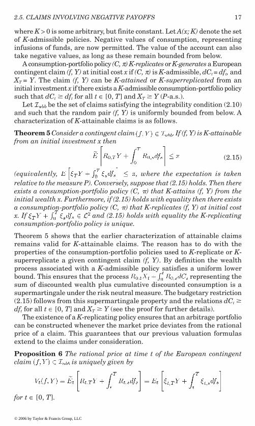
Theorem 5 Consider a contingent claim . If (f, Y) is K-attainablefrom an initial investment x then
(2.15)
(equivalently, , where the expectation is takenrelative to the measure P). Conversely, suppose that (2.15) holds. Then thereexists a consumption-portfolio policy (C, �) that K-attains (f, Y) from theinitial wealth x. Furthermore, if (2.15) holds with equality then there existsa consumption-portfolio policy (C, �) that K-replicates (f, Y) at initial costx. If and (2.15) holds with equality the K-replicatingconsumption-portfolio policy is unique.
Theorem 5 shows that the earlier characterization of attainable claimsremains valid for K-attainable claims. The reason has to do with theproperties of the consumption-portfolio policies used to K-replicate or K-superreplicate a given contingent claim (f, Y). By definition the wealthprocess associated with a K-admissible policy satisfies a uniform lowerbound. This ensures that the process representing thesum of discounted wealth plus cumulative discounted consumption is asupermartingale under the risk neutral measure. The budgetary restriction(2.15) follows from this supermartingale property and the relations dCt �dft for all t ∈ [0, T] and XT � Y (see the proof for further details).
The existence of a K-replicating policy ensures that an arbitrage portfoliocan be constructed whenever the market price deviates from the rationalprice of a claim. This guarantees that our previous valuation formulasextend to the claims under consideration.
Proposition 6 The rational price at time t of the European contingentclaim is uniquely given by
for t ∈ [0, T].
2.5. CLAIMS INVOLVING NEGATIVE PAYOFFS
© 2006 by Taylor & Francis Group, LLC

18 CHAPTER 2. EUROPEAN CONTINGENT CLAIMS
2.6 The Structure of Contingent Claims’ PricesThe price of the contingent claim, in earlier sections, was represented as alocal semimartingale with unspecified drift coefficient (see (2.12)).Intuitive arguments suggest that the drift of this price process ought to berestricted if the financial market is complete. We formalize this intuitionnext.
A self-financing consumption-portfolio policy induces a wealthprocess satisfying
subject to the initial condition . Moreover, selecting the particularpolicy yields the locally riskless account value
with same initial condition. Define the excess portfolio return as and let represent the set
of date t states in which et � 0. Consider the portfolio policy. This policy invests all the resources available in
the claim if e � 0 and shorts a similar amount in the opposite event. Theassociated wealth process satisfies or, equivalently,
A potential arbitrage portfolio can then be constructed by financing thispolicy at the locally riskfree rate. The initial cost of this new strategy isnull and the terminal cash flow equals
Clearly, this is an arbitrage portfolio if has positive l × P-measure (where l is Lebesgue measure): in this situation an investor wouldbe able to profit for sure without disbursing funds. The absence of arbitrageopportunities, in equilibrium, implies that {(t, �,) : et = 0 } must have fullmeasure. We summarize the implication of this condition in our next theorem.
Theorem 7 The return of the attainable contingent claim (f, Y) satisfiesthe spanning relation
where . If the underlying asset corresponds to the market portfolioof risky securities this relation coincides with the Capital Asset PricingModel (CAPM) which states that the expected excess return on any securityis proportional to the expected excess return of the market portfolio. The
© 2006 by Taylor & Francis Group, LLC
19
proportionality factor ß is the beta of the claim. If the underlying asset doesnot correspond to the market portfolio, but satisfies the CAPM, then a simpletransformation establishes that the CAPM still holds for the claim, i.e.,
where μmt is the drift of the market portfolio and ßm
the beta of the claim with respect to the market portfolio.
This theorem records two results. First, it states that the market price ofrisk implied by the price of any contingent claim is identical to the marketprice of risk implied by the underlying asset. This is an intuitive relationgiven the completeness of asset markets (risks ought to be priced identicallyacross securities). Second, it also states that the price of the claim isconsistent with general pricing principles characterizing equilibrium infrictionless markets. In that regard the theorem shows that the riskpremium of the claim satisfies the CAPM, in that it is proportional to therisk premium of the market portfolio of risky securities. Further insightsregarding this equilibrium relationship can be found in the original articlesof Sharpe [1964], Lintner [1965] and Mossin [1969], who developed thestatic version of the CAPM. The dynamic version, for markets with diffusionprice processes, can be found in Merton [1973b].
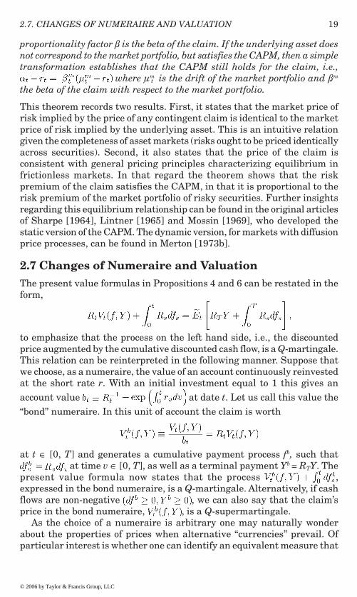
2.7 Changes of Numeraire and ValuationThe present value formulas in Propositions 4 and 6 can be restated in theform,
to emphasize that the process on the left hand side, i.e., the discountedprice augmented by the cumulative discounted cash flow, is a Q-martingale.This relation can be reinterpreted in the following manner. Suppose thatwe choose, as a numeraire, the value of an account continuously reinvestedat the short rate r. With an initial investment equal to 1 this gives an
account value at date t. Let us call this value the
“bond” numeraire. In this unit of account the claim is worth
at t ∈ [0, T] and generates a cumulative payment process fb, such that at time v ∈ [0, T], as well as a terminal payment Yb = RTY. The
present value formula now states that the process ,expressed in the bond numeraire, is a Q-martingale. Alternatively, if cashflows are non-negative , we can also say that the claim’sprice in the bond numeraire, , is a Q-supermartingale.
As the choice of a numeraire is arbitrary one may naturally wonderabout the properties of prices when alternative “currencies” prevail. Ofparticular interest is whether one can identify an equivalent measure that
2.7. CHANGES OF NUMERAIRE AND VALUATION
© 2006 by Taylor & Francis Group, LLC
20 CHAPTER 2. EUROPEAN CONTINGENT CLAIMS
preserves the martingale property in the new numeraire. The remainder ofthis section is devoted to these issues, first addressed in an insightful paperby Geman, El Karoui and Rochet [1995].
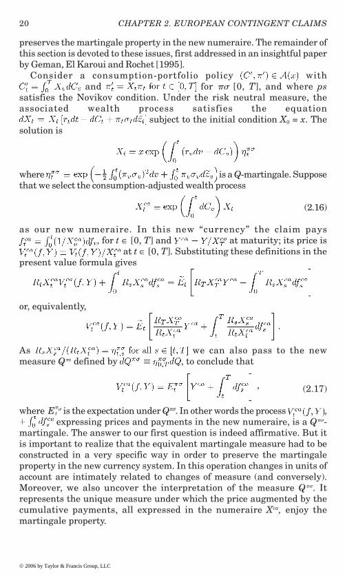
Consider a consumption-portfolio policy with and for �� [0, T], and where ps
satisfies the Novikov condition. Under the risk neutral measure, theassociated wealth process satisfies the equation
subject to the initial condition X0 = x. Thesolution is
where is a Q-martingale. Supposethat we select the consumption-adjusted wealth process
(2.16)
as our new numeraire. In this new “currency” the claim pays, for t ∈ [0, T] and at maturity; its price is
at t ∈ [0, T]. Substituting these definitions in thepresent value formula gives
or, equivalently,
As we can also pass to the newmeasure Q�s defined by , to conclude that
(2.17)
where E�t
� is the expectation under Qπσ. In other words the process , expressing prices and payments in the new numeraire, is a Q��-
martingale. The answer to our first question is indeed affirmative. But itis important to realize that the equivalent martingale measure had to beconstructed in a very specific way in order to preserve the martingaleproperty in the new currency system. In this operation changes in units ofaccount are intimately related to changes of measure (and conversely).Moreover, we also uncover the interpretation of the measure Q��. Itrepresents the unique measure under which the price augmented by thecumulative payments, all expressed in the numeraire Xca, enjoy themartingale property.
© 2006 by Taylor & Francis Group, LLC
,

21
A pricing relation, whose importance will become clear in the next section,can also be retrieved modulo an additional transformation. Fix t ∈ [0, T].Define, for s � t, the cash flow and let .As it follows from (2.17) that
(2.18)
This new expression shows that the value of the claim (f, Y) in the originaleconomy with interest rate r and risk neutral measure Q is identical to thevalue of the claim (f*, Y*) in a new economy with cumulative interest processC and risk neutral measure Q��. The result suggests a form of symmetrybetween the claims (f, Y) and (f*, Y*) when paired with their respectiveeconomies.
We can collect these results in the following theorem,
Theorem 8 Consider a European contingent claim (f, Y) ∈ and supposethat we adopt the new numeraire Xca defined in (2.16). Expressed in thisnew currency, the price of the claim, , augmented by the cumulativecash flow, , is a Qπσ -martingale where Qπσ is an equivalentmeasure with Q-density equal to (see (2.17)). Thevalue of the claim Vt(f, Y) in the original economy with interest rate r andpricing measure Q is the same as the value of a symmetric claim (f*, Y*), ina new economy with cumulative interest process C and pricing measure(i.e., equivalent martingale measure) Q��.
The symmetry property described in this proposition holds for anycontingent claim and, in particular, for the stock price (2.2). As we shallsee in the next sections and chapters, the result covers particular casesthat have been extensively studied in the options literature.
A discussion of general symmetry properties can be found in Kholodnyiand Price [1998]. Their analysis focuses on (2.17) and uses concepts fromoperator and group theories. They show, in particular, that symmetry canbe expressed in terms of Kelvin transforms. In their foreign exchangesetting the symmetry relations have a natural interpretation of payoffsfound on “opposite” sides of a market (i.e., payoffs quoted in differentcurrencies). Schroder [1999] applies the methodology of Geman, El Karouiand Rochet [1995] by selecting the dividend-adjusted asset price as thenew numeraire. This choice leads to a special case of (2.18), valid for generalclaims. Detemple [2001, Section 8] provides further perspective on thechange of measure and the symmetry property between seeminglyunrelated claims in different economies.
2.8 Option and Forward ContractsStandard European option contracts involve a payment at the maturitydate T only. For a call option the cumulative payment is f = 0 and the
2.8. OPTION AND FORWARD CONTRACTS
© 2006 by Taylor & Francis Group, LLC
.

22 CHAPTER 2. EUROPEAN CONTINGENT CLAIMS
terminal payoff is Y = (ST - K)+ where K is the strike price (or exercise price);for a put option f = 0 and Y = (K - ST)+. For these contracts the pricingformula of Proposition 4 specializes as follows.
Corollary 9 In the financial market model (2.1)–(2.2) the rational price of aEuropean call option with maturity date T and exercise price K is given by
for t ∈ [0, T]. The price of a European put option is ,for t ∈ [0, T].
Inspection of option payoffs reveals that the European put payoff is equalto the payoff of a call with matching characteristics minus the stock priceplus the strike price. That is, (K – ST)+ = (ST – K)+ +K – ST. The put value is thengiven by
(2.19)
This put-call parity (PCP) relationship determines the relative prices of optionswith identical characteristics written on the same underlying asset.
Another important property of options is the property of put-callsymmetry that relates the price of a put to the price of a call in an auxiliaryfinancial market with modified characteristics. To state this relationconsider a financial market with interest rate d, in which the underlyingasset price satisfies
(2.20)
under some risk neutral measure Q*. In this market the asset has dividendrate r and volatility coefficient �. The process z* is a Brownian motion underthe pricing measure Q*. Both z* and Q* are specified below. As before, thecoefficients (�, r, �) are adapted to the filtration F(.) generated by the Brownianmotion z, which represents the information available to investors.
Schroder [1999] demonstrates the following general European put-callsymmetry (PCS) property.
Theorem 10 (European PCS). Consider a European put option withcharacteristics K and T written on an asset with price S given by (2.2) inthe market with stochastic interest rate r. Let p(S, K, r, �; Ft) denote the putprice process. Then
p(S, K, r, �; Ft) = c(K, S, �, r; Ft) (2.21)
where c(K, S, �, r; Ft) is the value of a call with strike price S and maturity dateT in a financial market with interest rate δ and in which the underlying assetprice follows the Ito process (2.20) with initial value K and with z* defined by
(2.22)
© 2006 by Taylor & Francis Group, LLC
23
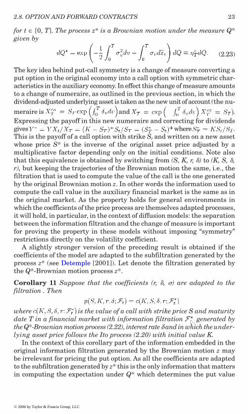
for t ∈ [0, T]. The process z* is a Brownian motion under the measure Q*given by
(2.23)
The key idea behind put-call symmetry is a change of measure converting aput option in the original economy into a call option with symmetric char-acteristics in the auxiliary economy. In effect this change of measure amountsto a change of numeraire, as outlined in the previous section, in which thedividend-adjusted underlying asset is taken as the new unit of account (the nu-
meraire is and .Expressing the payoff in this new numeraire and correcting for dividendsgives where .This is the payoff of a call option with strike St and written on a new assetwhose price S* is the inverse of the original asset price adjusted by amultiplicative factor depending only on the initial conditions. Note alsothat this equivalence is obtained by switching from (S, K, r, �) to (K, S, �,r), but keeping the trajectories of the Brownian motion the same, i.e., thefiltration that is used to compute the value of the call is the one generatedby the original Brownian motion z. In other words the information used tocompute the call value in the auxiliary financial market is the same as inthe original market. As the property holds for general environments inwhich the coefficients of the price process are themselves adapted processes,it will hold, in particular, in the context of diffusion models: the separationbetween the information filtration and the change of measure is importantfor proving the property in these models without imposing “symmetry”restrictions directly on the volatility coefficient.
A slightly stronger version of the preceding result is obtained if thecoefficients of the model are adapted to the subfiltration generated by the
the Q*-Brownian motion process z*.
Corollary 11 Suppose that the coefficients (r, �, �) are adapted to thefiltration . Then
where is the value of a call with strike price S and maturitydate T in a financial market with information filtration generated bythe Q*-Brownian motion process (2.22), interest rate δ and in which the under-lying asset price follows the Ito process (2.20) with initial value K.
In the context of this corollary part of the information embedded in theoriginal information filtration generated by the Brownian motion z maybe irrelevant for pricing the put option. As all the coefficients are adaptedto the subfiltration generated by z* this is the only information that mattersin computing the expectation under Q* which determines the put value
2.8. OPTION AND FORWARD CONTRACTS
© 2006 by Taylor & Francis Group, LLC
process z* (see Detemple [2001]). Let denote the filtration generated by

24 CHAPTER 2. EUROPEAN CONTINGENT CLAIMS
(see (2.34) in the appendix). Note that European PCS in the standard modelwith constant coefficients (the Black-Scholes setting) is a subcase of thiscorollary. Indeed, for this setting, it can be verified that the filtrations and F(.) coincide and that direct integration over z* leads to the call valuein the auxiliary financial market and the put value in the original economy.
Before turning our attention to forward contracts, note that we can alsouse the measure Q* in order to restate the European PCP relation as
Special cases of this formula (for instance in the setting with constantcoefficients) have been well documented in the literature.
A forward contract is another example of a derivative security, commonlyemployed to hedge financial exposures. This financial arrangement involvesa terminal payment Y = ST - K where K is the delivery price and has nointermediate cash flows (f = 0). Given that the final payment takes negativevalues, in the event ST < K, and is bounded below by -K the contract fits inthe framework of section 2.5.
Corollary 12 In the financial market model (2.1)–(2.2) the rational priceof a forward contract with maturity date T, delivery price K and written onthe asset price (2.2) is given by
for t ∈ [0, T], where Et* is the expectation under the measure Q* defined
above. The forward price f(t, S), representing the delivery price at which thecontract value is zero, is given by
for t ∈ [0, T].
2.9 Markets with Deterministic CoefficientsWhen the interest rate is constant, the price of an option written on anondividend-paying stock whose price follows a geometric Brownian motion
[1973a]).
Corollary 13 (Black and Scholes [1973]) Suppose that the interest rate ris constant and that the stock price follows a geometric Brownian motion
© 2006 by Taylor & Francis Group, LLC
process satisfies the Black and Scholes [1973] formula (see also Merton
.

25
process without dividends ((μ, �) constants, � = 0). Then the price of aEuropean call option simplifies to
(2.24)
where � � T - t is the time to maturity, N(.) is the cumulative standardnormal distribution function and .The price of a European put option with same maturity and exercise pricecan be obtained from the put-call parity relationship: ,or from the PCS property.
An explicit formula for the option can also be computed when the coefficientsof the model change deterministically over time.
Corollary 14 (Black-Scholes with deterministic coefficients) Consider thefinancial market model with deterministic interest rate, drift and volatilitycoefficients (rt, μt, �t) and without dividends (� = 0). Then, the price of aEuropean call option is given by
where N(.) is the cumulative standard normal distribution function and
The next result provides the price of a European option on a dividend-paying stock in a financial market with deterministic coefficients.
Corollary 15 (Black-Scholes with dividend adjustment) Consider thefinancial market model with deterministic interest rate, drift and volatilitycoefficients, and dividend rate (rt, μt, �t, �t). The price of a European calloption is given by
where , N(.) is the cumulative standard normaldistribution function and
(2.25)
2.9. MARKETS WITH DETERMINISTIC COEFFICIENTS
© 2006 by Taylor & Francis Group, LLC

26 CHAPTER 2. EUROPEAN CONTINGENT CLAIMS
Figure 2.1 shows the behavior of the call price function when the coefficientsr, �, � are constants. Convexity with respect to the underlying assetprice is apparent. This property can be easily proved from the convexityof the payoff function. The call price converges to zero as the underlyingprice converges to zero, reflecting the vanishing probability of exercise.At the other extreme, the call price converges to the discounted valueof the difference between the asset price and the strike,
. For intuition note that theprobability of exercise converges to one as St becomes large and thereforethat the call value converges to the present value of ST - K. As the call priceis non-negative and the call payoff dominates ST - K, we also have thelower bound .
For risk management purposes it is important to identify the sensitivityof the option price with respect to the underlying asset price. The delta
Figure 2.1: Black-Scholes model. This figure graphs the European call price ct, thepayoff function (St - K)+ and the lower bound max (y-axis) with respect to the underlying asset price (x-axis). Parameter values are r= 2%, � = 6%, � = 0.25 and T - t = 1.
© 2006 by Taylor & Francis Group, LLC

27
hedge of the option, given by the derivative , quantifies thissensitivity. In the context of the model with dividend adjustment oneobtains,
Corollary 16 Consider the model with dividend adjustment of Corollary15 and let c(S, t) denote the value of the European call option. The deltahedge ratio is
with d as in (2.25).
Figure 2.2 graphs the delta hedge ratio as a function of the underlyingasset price. As expected the delta hedge converges to zero as S approacheszero and to e–�(T–t) as S becomes large. Convexity of the price function ensuresthat h(St, t) is bounded above by e–�(T–t).
Figure 2.2: Hedging in the Black-Scholes model. This figure displays the behaviorof the call hedge ratio ht (y-axis) with respect to the underlying asset price (x-axis).Parameter values are r = 2%, � = 6%, σ = 0.2 and T - t = 1. The upper bound ise-�(T - t).
2.9. MARKETS WITH DETERMINISTIC COEFFICIENTS
© 2006 by Taylor & Francis Group, LLC

28 CHAPTER 2. EUROPEAN CONTINGENT CLAIMS
To complete this section we record the value of a forward contract in thesimple setting of Corollary 15. This formula and the correspondingexpression for the forward price follow immediately from Corollary 12 andare straightforward adaptations of standard results (see, for instance, Hull[2002]).
Corollary 17 Consider the model with dividend adjustment of Corollary15 and let vf(S, t) denote the value of a forward contract with delivery dateT, delivery price K and written on the asset price S. Then
for t ∈ [0, T]. The forward price is for t ∈[0, T].
Lastly, we point out that all the results in this section are also valid whenthe coefficient μ of the asset price process is an adapted stochastic process.In the risk neutral environment only the properties of the interest rateand of the volatility of the asset return matter for pricing payoffs that arenot explicitly tied to the drift of the asset return. As long as r and s areconstants, or deterministic functions of time, the formulas displayed abovewill apply.
2.10 Markets with Multiple AssetsWe now outline an extension to a financial market with d risky securities.The underlying sources of uncertainty are represented by a d-dimensionalvector of Brownian motion processes z. There is a riskless asset payinginterest at the rate r where r is a positive, bounded and progressivelymeasurable process. The vector of risky asset prices S satisfies
(2.26)
where IS is a d × d diagonal matrix with vector of prices on its diagonal, �is a d × 1 vector of dividend rates, μ is a d × 1 vector of drifts and � a d × dmatrix of volatility coefficients. All the coefficients are progressivelymeasurable and bounded processes; the dividends are non-negative. Wealso assume that the volatility matrix � is invertible and that the d-dimensional MPR process satisfies the Novikov condition
where . This last assumption ensures that the exponentialprocess
(2.27)
© 2006 by Taylor & Francis Group, LLC

29
is a martingale and that the measure, , is aprobability measure equivalent to P; Q is the equivalent martingalemeasure in the multiasset case.
All the definitions, properties and results demonstrated in the contextof the single asset model generalize naturally to this multiasset financialmarket. In particular the value of a contingent claim can be written as thepresent value of its future discounted cash flows.
Proposition 18 The rational price at time t of the European contingentclaim (f, Y) ∈ is uniquely given by
for t ∈ [0, T] where is defined in (2.27) and where .
The rational price of the contingent claim is calculated by discounting cashflows either at the riskfree rate (under the risk neutral measure) or at therisk-adjusted rate embedded in the SPD � (under the original measure).The structures of these valuation formulas are identical to those in thesingle asset case. Analogs of Proposition 6 and Theorem 7 also hold in thismultiasset setting.
2.11 Appendix: ProofsProof of Theorem 1: Detailed proofs can be found in Karatzas and Shreve[1988], [1998]. Our demonstration below provides the key elements in thederivation of this central result.
Consider a consumption-portfolio policy (C, �) and let X be the wealthprocess generated by (C, �). An application of Ito’s lemma gives
(2.28)
for all t ∈ [0, T].(i) Necessity: Suppose now that the policy is admissible: .
The right-hand side of (2.28) is a continuous local martingale. Admissibilityof (C, �) implies that the left-hand side of (2.28) is non-negative. Thecombination of these two properties implies that the right-hand side is anon-negative supermartingale (Karatzas and Shreve [1988, Chapter 1,Problem 5.19]). Taking expectations on both sides of (2.28) and setting t =T then yields
Hence if (f, Y) is attainable (XT � Y and dCt � dft for all t ∈ [0, T]) frominitial wealth x then
2.11. APPENDIX: PROOFS
© 2006 by Taylor & Francis Group, LLC
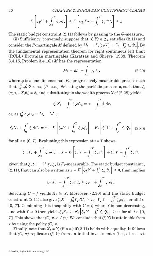
30 CHAPTER 2. EUROPEAN CONTINGENT CLAIMS
The static budget constraint (2.11) follows by passing to the Q-measure..(ii) Sufficiency: conversely, suppose that (f, Y) ∈ satisfies (2.11) and
consider the P-martingale M defined by . By
the fundamental representation theorem for right continuous left limit(RCLL) Brownian martingales (Karatzas and Shreve [1988, Theorem3.4.15, Problem 3.4.16]) M has the representation
(2.29)
where � is a one-dimensional, F(.)-progressively measurable process such
that . Selecting the portfolio process �t such that �s
(�s�s – Xss) = �s and substituting in the wealth process X of (2.28) yields
or, as ,
(2.30)
for all t ∈ [0, T]. Evaluating this expression at t = T shows
given that is FT-measurable. The static budget constraint ,
(2.11), that can also be written as , then implies
Selecting C = f yields XT � Y. Moreover, (2.30) and the static budget
constraint (2.11) also give for all t ∈[0, T]. Combining this inequality with C = f, where f is non-decreasing,
and with Y � 0 then yields , for all t ∈ [0,
T]. This shows that (C, �) ∈ A(x). We conclude that (f, Y) is attainable from
x by using the policy (C, �).Finally, note that XT = Y, (P-a.s.) if (2.11) holds with equality. It follows
that (C, �) replicates (f, Y) from an initial investment x (i.e., at cost x).
© 2006 by Taylor & Francis Group, LLC

31
When the martingale M, defined above, is square-integrable. The process � in the representation (2.29) is then unique. Theuniqueness of the replicating consumption-portfolio policy follows. �
Proof of Proposition 4: The contingent claim (f, Y) is attainable from allinitial investments x satisfying the budget constraint (2.11). Minimizingover this set yields the (unique) minimum investment from which (f, Y) is
attainable: . Let (C, �) be the replicating
strategy and X the associated wealth process. Note that withdrawalsassociated with this replicating policy can be reinvested in the account. Inthis case the balance of the account evolves according to dX + dC. To provethe proposition we show that for t = 0. A straightforwardadaptation of the argument will then establish the result for an arbitrarytime t ∈ [0, T].
So let us first suppose that . Under this condition thestrategy of selling (f, Y) at a price V0(f, Y), and undertaking the policy (C, π)that generates (f, Y) from initial wealth x*, is an arbitrage opportunity. Indeed,this strategy produces an immediate inflow equal to V0(f, Y) – x* > 0 andsubsequent cash flows equal to and XT - Y = 0. Thewealth process associated with the strategy is
with initial condition , as no external cash infusions are needed tostart the strategy. Solving this stochastic differential equation yields
To preclude this
arbitrage it must be the case that .Assume then that V0(f, Y) < x*. In this instance, buying the claim and
investing in the replicating portfolio yields cash flows x* – V0(f, Y) > 0,dCt – dCt – dft = 0 and XT - Y = 0. This is again an arbitrage strategy, by thesame arguments. We conclude that V0(f, Y) = x* to preclude the existenceof arbitrage opportunities.
As the sum of discounted wealth plus cumulative discountedconsumption is a Q-martingale, a similar reasoning establishes that theminimum amount of wealth needed at date t to generate (f, Y) is
. The price of the claim at date t follows. �
Proof of Theorem 5: The discounted wealth process generated by a policy(C, �) satisfies
(2.31)
for all t ∈ [0, T]. If we use the state price density as a deflator we obtainthe alternative expression (2.28).
2.11. APPENDIX: PROOFS
© 2006 by Taylor & Francis Group, LLC

32 CHAPTER 2. EUROPEAN CONTINGENT CLAIMS
(i) Necessity: Suppose now that the policy is K-admissible: (C, �) ∈ A(x;K). The right-hand side of (2.31) is a continuous Q-local martingale. K-admissibility of (C, �) and boundedness of the interest rate imply that theleft-hand side is bounded below. We conclude that the right-hand side is asupermartingale. Taking the Q-expectation on each side and setting t = Tthen yields
Hence if (f, Y) is K-attainable (XT � Y and dCt � dft for all t ∈ [0, T]) frominitial wealth x then
which establishes the budget constraint (2.15).
(ii) Sufficiency: conversely, suppose that satisfies (2.15) and
consider the P-martingale M defined by .
Proceeding along the same lines as in the proof of Theorem 1 leads to
(2.32)
for all t ∈ [0, T]. Evaluating this expression at t = T establishes
given that is FT-measurable. The budget constraint (2.15)then implies
Selecting C = f yields XT � Y. Moreover, (2.32) and the static budgetconstraint (2.15) also give for all t ∈[0, T]. As C = f we can also write
for all t ∈ [0, T]. Given that r is bounded and (f, Y) is bounded from below,the random variable is bounded from below as well. Itthen follows that Xt � – K for all t ∈ [0, T]. We conclude that (C, �) ∈ A(x;K) and that the policy (C, �) K-superreplicates the claim (f, Y). Note alsothat XT = Y, (P-a.s.) if (2.15) holds with equality. In this case (C, �) is seen toK-replicate (f, Y) at cost x.
© 2006 by Taylor & Francis Group, LLC

33
The last statement is proved as in Theorem 1. �
Proof of Proposition 6: The proof parallels the proof of Proposition 4. Set
and note that Theorem 5 ensures the existence
of a K-replicating consumption-portfolio policy starting from initial wealthx*. The same no-arbitrage argument can then be applied to show that V0(f,Y) = x*. �
Proof of Theorem 7: The no-arbitrage argument sketched in the text showsthat
It follows immediately that where βt≡ρt/σt.If the underlying asset satisfies the CAPM then
where μm, �m are the coefficients of the process followed by the price of themarket portfolio of risky assets. Simple algebra establishes that t – rt = �m
t
(μmt – rt) where . �
Proof of Theorem 8: The proof is outlined in the text leading up to theproposition. �
Proof of Corollary 9: Substitution of the call and put payoff functions inthe formula of Proposition 4 yields the results stated. �
Proof of Theorem 10: Let be the price of the put optionwith characteristics (K, T), in the original financial market. This price hasthe (present value) representation
where and the expectation is taken relative to theequivalent martingale measure Q. Simple manipulations show that theright hand side of this equation equals
(2.33)
where .Consider the new measure , which is equivalent to Q.
Girsanov’s Theorem (Karatzas and Shreve [1988, Theorem 5.1]) implies
2.11. APPENDIX: PROOFS
© 2006 by Taylor & Francis Group, LLC

34 CHAPTER 2. EUROPEAN CONTINGENT CLAIMS
that the process is a Q*-Brownian motion. Substitutingz* in (2.33) and passing to the measure Q* yields
(2.34)
where denotes the conditional expectation relative to Q*. But the righthand side is the value of a call option with strike S, maturity date T in aneconomy with interest rate δ and pricing measure Q*. The underlying assetprice is
at date T. An application of Ito’s lemma shows that satisfies (2.20), for allv ∈ [t, T], with initial condition . Inspection of this equation showsthat the asset pays dividends at the rate r in the economy with interest rate� and risk neutral measure Q*. �
Proof of Corollary 11: When the coefficients (r, �, �) are adapted to thefiltration F(t)
* the conditional expectation in (2.34) with respect to the sigma-algebra Ft is the same as the conditional expectation with respect to ,for all t ∈ [0, T]. The result follows. �
Proof of Corollary 12: An application of Proposition 6 shows that Vt = Et
[Rt,T(ST – K)]. Using the stock price formula (2.8) establishes that Vt = St –
. Solving the linear SDE (2.2) and passing
to the Q-measure gives
and, with the definition of the measure Q*,
Substituting in and simplifying gives
© 2006 by Taylor & Francis Group, LLC

35
The forward price f(t, S) is obtained by solving the equation
for f(t, St). �
Proof of Corollary 13: Let � = T - t. The call option price in Proposition 4can be written as
Under the risk neutral measure Q the stock price is
where z~T – z~t is distributed as z~�—T–t
— and z~ is a standard normal random
variable. Thus,
(2.35)
where N(.) is the cumulative standard normal distribution. The firstexpectation is
(2.36)
where E*t[.] is the expectation under Q* in (2.23), specialized to the case
under consideration. Under this measure the asset price is distributed as
where z* is a standard normal variate. An adaptation of the computationin (2.35), to account for the new measure Q*, shows that (2.36) equals erτ
StN(d). Combining (2.35) and (2.36) gives (2.24).To prove the put-call parity relationship, note that (K - ST)+ = (ST - K)+ -
ST + K. No arbitrage implies that the value of the put must equal the valueof the portfolio of the securities on the right-hand side of the equality. Theparity relationship follows. �
Proof of Corollary 14: Under the assumptions stated we have
2.11. APPENDIX: PROOFS
© 2006 by Taylor & Francis Group, LLC
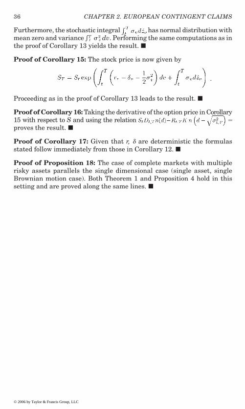
36 CHAPTER 2. EUROPEAN CONTINGENT CLAIMS
Furthermore, the stochastic integral has normal distribution withmean zero and variance �T
t �2v dv. Performing the same computations as in
the proof of Corollary 13 yields the result. �
Proof of Corollary 15: The stock price is now given by
Proceeding as in the proof of Corollary 13 leads to the result. �
Proof of Corollary 16: Taking the derivative of the option price in Corollary15 with respect to S and using the relation proves the result. �
Proof of Corollary 17: Given that r, � are deterministic the formulasstated follow immediately from those in Corollary 12. �
Proof of Proposition 18: The case of complete markets with multiplerisky assets parallels the single dimensional case (single asset, singleBrownian motion case). Both Theorem 1 and Proposition 4 hold in thissetting and are proved along the same lines. �
© 2006 by Taylor & Francis Group, LLC
.

37
Chapter 3
American ContingentClaims
We now turn our attention to the valuation of American contingent claims.By definition these are contracts that can be exercised during certainprespecified periods of time, at the option of the holder. Their valuation,naturally, requires the determination of the optimal exercise policy. Theabsence of arbitrage opportunities implies that the value of the contract isthe value under the optimal exercise policy.
This chapter presents several approaches that can be used to priceAmerican-style contingent claims. The analysis is cast in the generalfinancial market model with Ito price processes and adapted interest rateprocess. The results described will be used in subsequent chapters to studymore specific contractual forms, such as vanilla options, barrier and cappedoptions, multiasset options and occupation time derivatives, in marketswith constant coefficients. They also serve as starting points for some of
In a preliminary step we extend the valuation formula in Proposition 4to securities with payoffs at random times (section 3.1). We then valueAmerican contingent claims (sections 3.2 and 3.3) and specialize the resultsto options (section 3.5). The case of financial markets with multiple assetsis considered last (section 3.6).
3.1 Contingent Claims with Random Maturity
The economic setting is the one presented in section 2.2. In order to describeclaims with random timing of payments we need to introduce a fewadditional concepts. A random time τ is a stopping time of the (Brownian)filtration F(�) if the event {τ ≤ t} belongs to the σ-field Ft for every t ∈ [0, T].In other words τ is a stopping time if, at any time t, an individual observingthe underlying source of uncertainty (thus endowed with the σ-algebra Ft)
© 2006 by Taylor & Francis Group, LLC
the numerical methods presented in chapter 8.

CHAPTER 3. AMERICAN CONTINGENT CLAIMS38
can tell whether τ has occurred or not. Let S0,Τ denote the set of stoppingtimes taking values in [0, T].
Consider a contingent claim (f, Y) and an exogenously specified stoppingtime τ ∈ S0,T. Here f is a cumulative payment process up to τ: this finitevariation process is non-decreasing, progressively measurable, right-continuous and null at zero. Also, Y is used to represent a terminal, non-negative and Ft-measurable cash flow Yτ paid at the random time τ. Toprepare the ground for the case of American claims we can actually thinkof Y as a right-continuous, adapted stochastic process with value Yτ at therandom maturity date τ. By analogy with condition (2.10) in section 2.2we consider claims (f, Y) satisfying the integrability condition1
(3.1)
Let be the class of claims that satisfy this condition and df ≥ 0, Y ≥ 0.
Theorem 19 Let τ be a stopping time in S0,T and suppose that .
The rational price of this contingent claim, Vt(f, Y, τ), is uniquely given by
for all t ∈ [0, τ].
This result shows that contingent claims that expire at a stopping time ofthe filtration are valued in the same manner (using the same pricingoperator) as contracts with fixed maturity date. The key ingredient is thefact that the random maturity is a function of the Brownian motion thatgenerates the information structure. The completeness of the financialmarket (relative to this Brownian motion) ensures that maturity risk canbe properly hedged. The absence of arbitrage opportunities validates theequality between the price of the claim and the value of the replicatingportfolio.
Note that the class of claims covered by Theorem 19 includes contractspaying cash flows at multiple random dates. These discrete payments are, infact, embedded in the cumulative cash flow process f, which may includediscontinuities at random times. Letting Δf be the jumps in f we can write f =fc + fd where fc is the purely continuous part of the cumulative payment processand fd =Σ Δf its purely discontinuous part. The valuation formula can then be
1Note that the supremum inside the expectation is taken path-by-path. Condition (3.1),therefore, implies that sup , where is thedeflated payoff process.
© 2006 by Taylor & Francis Group, LLC
.

39
restated as
where τj is the random time of the jth-jump in the interval [t, τ]. This resultis already implicit in the formulas provided in the previous chapter, whichtreat the special case τ=T.
3.2 American Contingent ClaimsIf, instead of being exogenously specified, the stopping time τ can be chosenby the holder of the claim, then (f, Y) is an American-style contingent claim.A stopping time is also called an exercise time or exercise policy for theclaim. In fact, as the choice of an exercise time can only be based on theinformation available (and given that information is assumed to behomogeneous among participants in the financial market), the class ofexercise policies available to the claimholder naturally coincides with theclass of stopping times of the filtration. The decision to exercise can thenbe thought of as the selection of the best stopping time τ with values in [0,T], i.e., the one that maximizes the value of the claim for the owner. Thisis the optimal exercise policy.
In order to state the first pricing result we introduce the followingnotation. For t ∈ [0, T] define the deflated payoff process
(3.2)
where is the state price density introduced in chapter 2. Tosimplify matters, assume that D is a continuous process, for the remainderof this chapter. Consider the associated process Z such that
(3.3)
which is known as the Snell envelope of D. The process Z plays an importantrole in the characterization of the optimal exercise time and the valuation
that Z is a supermartingale with a right-continuous left-limit modification.2
2To see the supermartingale property let τt be the optimal stopping time for Zt and notethat , for all s ≥ t.
3.2. AMERICAN CONTINGENT CLAIMS
© 2006 by Taylor & Francis Group, LLC
of the American claim. It has a number of useful properties (see El Karoui
Clearly Z is non-negative as D is non-negative. In fact, it can be shown[1981] and Karatzas and Shreve [1998, Appendix D] for detailed analyses).

CHAPTER 3. AMERICAN CONTINGENT CLAIMS40
Below, we will assimilate it with its modification. It is also a majorant ofD: as τ = t is a stopping time in St,T we obviously have Zt ≥ Dt, for all t ∈ [0,T]. In fact Z is the smallest supermartingale majorant of D (i.e., it isbounded above by any supermartingale that majorizes D).3 Finally, foreach t ∈ [0, T], the optimization problem on the right hand side of (3.3) issolved by the stopping time
(3.4)
(as Zs = Ds means that immediate exercise is optimal at s). Given that D iscontinuous and (because ) a solution
exists (see Karatzas and Shreve [1998, Appendix D]). With these definitionswe are in a position to identify the value of an American contingent claim.
Theorem 20 (Bensoussan [1984], Karatzas [1988]). Consider an American-style contingent claim ). For all t ∈ [0, τ0] the value of the claim,
Vt(f, Y), is uniquely given by
(3.5)
The optimal exercise policy is given by
(3.6)
Note that the right hand side of (3.5) can also be written relative to theQ-measure as
Thus, the theorem formalizes the intuitive notion that the value of anAmerican contingent claim ought to equal the highest value that can beachieved by selecting exercise policies in the feasible set. In effect theproof demonstrates the existence of an admissible consumption-portfoliopolicy that replicates the right hand side of (3.5). The value of the claim isthe value of this replicating policy. Formula (3.5) also demonstrates thatthe same pricing principles, as in the case of European claims or claimswith exogenously specified random maturity, apply.
Theorem 20 suggests a separation of the valuation problem into twosteps. The first step consists in solving the auxiliary problem embedded inthe definition of the Snell envelope (3.3). This problem is well defined forall times t∈ [0, T]. Its resolution produces the supermartingale Z alongwith the set of stopping times (3.4) indexed by t. In the second step thevaluation problem is expressed in terms of the Snell envelope. The optimalexercise policy is the specific stopping time τ0, i.e., the first time in the
3Let S be an arbitrary supermartingale majorant of D. Then, for any τ ∈ St,T we haveEτDτ≤EτSτ≤Sτ, where the first inequality follows from the majorizing property of S and thesecond one from the supermartingale property of S. Optimizing over the set of stoppingtimes St,T establishes that Zt ≤ St.
© 2006 by Taylor & Francis Group, LLC
.

41
interval [0, T] at which the Snell envelope equals the discounted payoff D.The value of the American-style contingent claim prior to this exercisedate is the value under this exercise policy. In a rational financial marketthe American contingent claim issued at date 0 matures endogenously atthis exercise time.
Remark 3 The actualized cash flow-corrected Snell envelope
(3.7)
prices newly issued claims at any point in time t ∈ [0, T]. For example, anAmerican contingent claim (f, Y) marketed (or remarketed) at time t ≥ τ0
and whose cash flows are those in the original contract that pertain to the
sub-period [t, T] is worth . The optimalexercise time is the first time post-introduction at which the Snell envelopeequals the deflated payoff of the claim . If tt >t the newly issued claim will survive until its endogenous expiration date.If τt=t immediate exercise is optimal: the claim has no material existence.A claim that is continuously marketed (or quoted) during the period [0, T]carries a price given by (3.7). This provides further motivation for the studyof the Snell envelope.
Remark 4 For claims (0,Y) consisting solely of a terminal payoff, Theorem20 states that for t ≤ τ0. Oneconcludes immediately that the discounted price, R0,tVt, of an Americancontingent claim without intermediate payments is a Q-martingale prior tothe optimal exercise time (where discounting is at the riskfree rate). Forclaims with intermediate cash flows it is the discounted priceaugmented by the sum of discounted intermediate cash flows that has theQ-martingale property.
Although intuitive, the representation of the price provided in (3.5)–(3.6)is incomplete, because the optimal stopping time defined via the Snell envelopeis not expressed in an explicit form. A further characterization of this optimalpolicy is therefore needed to proceed with valuation. A decomposition, thatbuilds upon the Snell envelope and emphasizes the gains from early exercise(prior to the maturity date T), proves useful in that regard. It often producesadditional insights about the price structure of an American claim and leadsto a characterization of the optimal exercise time that can be exploited inspecialized contexts. This decomposition is examined next.
3.3 Exercise Premium RepresentationsThe formula identifying the gains realized by optimally exercising before thematurity date of the contract is known as the early exercise premiumrepresentation (EEP) of the American contingent claim price. The EEP formularelates to a general result valid for a large class of supermartingales, known as
3.3. EXERCISE PREMIUM REPRESENTATIONS
© 2006 by Taylor & Francis Group, LLC
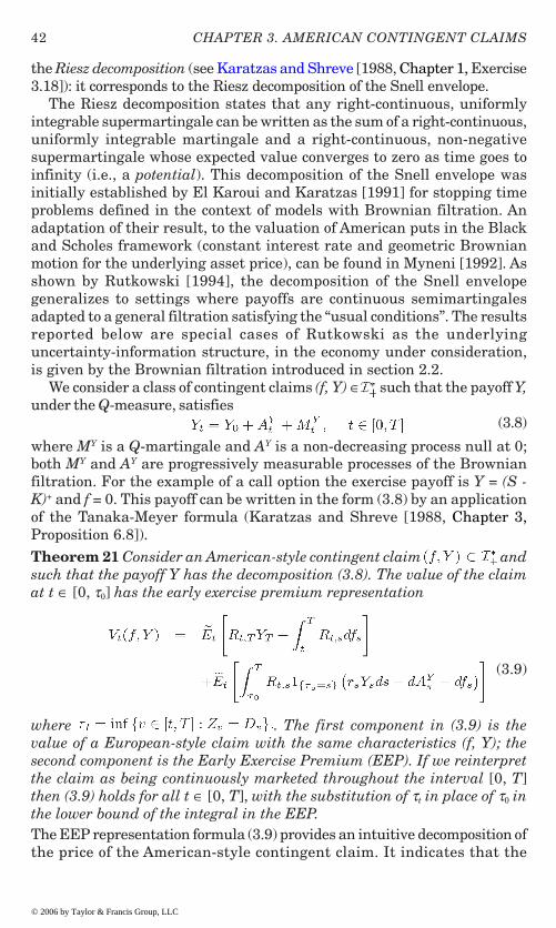
CHAPTER 3. AMERICAN CONTINGENT CLAIMS42
the Riesz decomposition (see Karatzas and Shreve [1988, Chapter 1, Exercise3.18]): it corresponds to the Riesz decomposition of the Snell envelope.
The Riesz decomposition states that any right-continuous, uniformlyintegrable supermartingale can be written as the sum of a right-continuous,uniformly integrable martingale and a right-continuous, non-negativesupermartingale whose expected value converges to zero as time goes toinfinity (i.e., a potential). This decomposition of the Snell envelope wasinitially established by El Karoui and Karatzas [1991] for stopping timeproblems defined in the context of models with Brownian filtration. Anadaptation of their result, to the valuation of American puts in the Blackand Scholes framework (constant interest rate and geometric Brownianmotion for the underlying asset price), can be found in Myneni [1992]. Asshown by Rutkowski [1994], the decomposition of the Snell envelopegeneralizes to settings where payoffs are continuous semimartingalesadapted to a general filtration satisfying the “usual conditions”. The resultsreported below are special cases of Rutkowski as the underlyinguncertainty-information structure, in the economy under consideration,is given by the Brownian filtration introduced in section 2.2.
We consider a class of contingent claims (f, Y) ∈ such that the payoff Y,under the Q-measure, satisfies
(3.8)
where MY is a Q-martingale and AY is a non-decreasing process null at 0;both MY and AY are progressively measurable processes of the Brownianfiltration. For the example of a call option the exercise payoff is Y = (S -K)+ and f = 0. This payoff can be written in the form (3.8) by an applicationof the Tanaka-Meyer formula (Karatzas and Shreve [1988, Chapter 3,Proposition 6.8]).
Theorem 21 Consider an American-style contingent claim andsuch that the payoff Y has the decomposition (3.8). The value of the claimat t ∈ [0, τ0] has the early exercise premium representation
(3.9)
where . The first component in (3.9) is thevalue of a European-style claim with the same characteristics (f, Y); thesecond component is the Early Exercise Premium (EEP). If we reinterpretthe claim as being continuously marketed throughout the interval [0, T]then (3.9) holds for all t ∈ [0, T], with the substitution of τt in place of τ0 inthe lower bound of the integral in the EEP.The EEP representation formula (3.9) provides an intuitive decomposition ofthe price of the American-style contingent claim. It indicates that the
© 2006 by Taylor & Francis Group, LLC

43
price of the contract is the value of a European contingent claim with matchingcharacteristics augmented by the present value of the gains from early exercise(the early exercise premium). The (local) gains from early exercise are givenby the cash flow . The first component, rsYsds, representsthe interest collected over the next increment of time, by exercisingimmediately and placing the proceeds in the riskless account (this is also theopportunity cost saved by exercising immediately instead of waiting, i.e., thetime value of money embedded in the discount rate r). The second component,– , is the loss incurred, upon exercise, due to the natural appreciation ofthe payoff Y. Indeed, by exercising, the claimholder forgoes further appreciationin the payoff. The last component, -dfs, is the loss incurred, upon exercise, byforgoing the cash flow paid by the claim. As we shall see in the next sectionthe early exercise premium and the gains from early exercise have a morespecialized interpretation in the case of an American option.
The EEP representation provides useful insights into the determinants ofthe exercise decision. The following result is a direct consequence of theformula.
Corollary 22 Contingent claims such that forall v ∈ [0, T] will never be exercised prior to the maturity date.
Under the condition of the Corollary the net benefit of exercising isnon-positive at all times. As a result, incentives to exercise are insufficientand the early exercise premium will be null. A special case of this result isobtained when the claim is a call option on a non-dividend-paying stock.It is well known that it is suboptimal to exercise an American call prior tomaturity under these conditions (Merton [1973a]). For this contract Y =(S - K)+ and f = 0, and, in the exercise region where S > K, we have
. Corollary 22 thenapplies and shows that early exercise is a suboptimal policy as it can onlyreduce the value of the contract.
A complement to the EEP representation of an American contingentclaim is a decomposition emphasizing the gains from delaying exercise.This formula is known as the delayed exercise premium representation(DEP). The DEP of an American put option on a non-dividend-paying assetand in a financial market with constant coefficients (constant interestrate and geometric Brownian motion for the stock price) was derived byCarr, Jarrow and Myneni [1992]. The next theorem extends their analysisto the more general class of American claims discussed in this section.
Theorem 23 Consider an American-style contingent claim andsuch that the payoff Y has the decomposition (3.8). The value of the claimat t ∈ [0, τ0] has the delayed exercise premium representation
(3.10)
3.3. EXERCISE PREMIUM REPRESENTATIONS
© 2006 by Taylor & Francis Group, LLC

CHAPTER 3. AMERICAN CONTINGENT CLAIMS44
where . The first component in (3.10) is theimmediate exercise value; the second one is the Delayed Exercise Premium(DEP). If we reinterpret the claim as being continuously marketed throughoutthe interval [0, T] then (3.10) holds for all t ∈ [0, T], with the substitution ofτt in place of τ0 in the indicator function appearing in the DEP.
The delayed exercise premium representation can be viewed as the counterpartof the EEP representation to the extent that it emphasizes the gains fromwaiting to exercise. The net gains consist of three parts: the appreciation ofthe payoff the cash inflow collected dfs and the interest foregone bypostponing exercise -rsYsds (an opportunity cost). The present value of thesegains is captured by the second component on the right hand side of (3.10).This value component is also known as the time value of the contingentclaim.
3.4 A Duality Formula: Upper Price BoundsThe Snell envelope (3.3) and the valuation formula (3.5) immediately suggestthat the price of an American-style contingent claim is bounded below by
where τ is any arbitrary stopping time in S0,T. This simple insight will, infact, be exploited in chapter 8, in order to manufacture interesting lower boundapproximations for option prices. The deduction of an upper bound for theclaim’s price is much less evident, but nevertheless feasible. It relies on dualityresults established by Davis and Karatzas [1994] and Rogers [2002].
Theorem 24 (Davis and Karatzas [1994], Rogers [2002]) Consider anAmerican-style contingent claim . The value of the claim, V0(f,Y), is given by
(3.11)
where is the space of P-martingales that are null at t = 0 and suchthat
Theorem 24 shows that the claim’s price is bounded above by
where M is any arbitrary martingale that is integrable in the sense of. Taking the minimum upper bound over this class, in fact, produces
the price of the claim. Thus, instead of maximizing over a class of stoppingtimes one can, equivalently, minimize over a set of martingales, in orderto price the claim.
The reasons underlying this duality formula are deep. It is fairly clearthat the quantity is an upper bound for the price, as it
© 2006 by Taylor & Francis Group, LLC
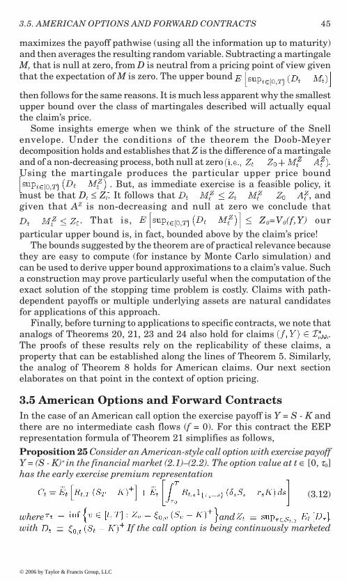
45
maximizes the payoff pathwise (using all the information up to maturity)and then averages the resulting random variable. Subtracting a martingaleM, that is null at zero, from D is neutral from a pricing point of view giventhat the expectation of M is zero. The upper bound
then follows for the same reasons. It is much less apparent why the smallestupper bound over the class of martingales described will actually equalthe claim’s price.
Some insights emerge when we think of the structure of the Snellenvelope. Under the conditions of the theorem the Doob-Meyerdecomposition holds and establishes that Z is the difference of a martingaleand of a non-decreasing process, both null at zero .Using the martingale produces the particular upper price bound
. But, as immediate exercise is a feasible policy, itmust be that Dt ≤ Zt. It follows that , andgiven that AZ is non-decreasing and null at zero we conclude that
. That is, Z0=V0(f,Y) our
particular upper bound is, in fact, bounded above by the claim’s price!The bounds suggested by the theorem are of practical relevance because
they are easy to compute (for instance by Monte Carlo simulation) andcan be used to derive upper bound approximations to a claim’s value. Sucha construction may prove particularly useful when the computation of theexact solution of the stopping time problem is costly. Claims with path-dependent payoffs or multiple underlying assets are natural candidatesfor applications of this approach.
Finally, before turning to applications to specific contracts, we note thatanalogs of Theorems 20, 21, 23 and 24 also hold for claims .The proofs of these results rely on the replicability of these claims, aproperty that can be established along the lines of Theorem 5. Similarly,the analog of Theorem 8 holds for American claims. Our next sectionelaborates on that point in the context of option pricing.
3.5 American Options and Forward ContractsIn the case of an American call option the exercise payoff is Y = S - K andthere are no intermediate cash flows (f = 0). For this contract the EEPrepresentation formula of Theorem 21 simplifies as follows,
Proposition 25 Consider an American-style call option with exercise payoffY = (S - K)+ in the financial market (2.1)–(2.2). The option value at t ∈ [0, τ0]has the early exercise premium representation
(3.12)
where and .with If the call option is being continuously marketed
3.5. AMERICAN OPTIONS AND FORWARD CONTRACTS
© 2006 by Taylor & Francis Group, LLC

CHAPTER 3. AMERICAN CONTINGENT CLAIMS46
throughout the interval [0, T] then (3.12) holds for all t ∈ [0, T], with thesubstitution of τt in place of τ0 in the EEP.
Under the risk neutral measure the drift of the underlying asset price (2.2)is given by Ss(rs - δs)ds. In the exercise region we must have S > K. It followsthat the local gains from exercise of a call option are given by
in the event {τs = s}. These gains are equal to the dividend benefits collectedupon receipt of the underlying asset net of the interest forgone on the cashpaid to exercise the option. The optimal exercise time is determined bythe super-martingale Z corresponding to the deflated option payoff. Clearly,the payment of dividends on the underlying asset provides incentives forearly exercise. Intuition suggests that immediate exercise will take placewhen these incentives are sufficiently large.
For American options the simple put-call parity relation (2.19) forcontracts with identical characteristics (T, K) fails. Indeed, the optimalexercise policies associated with the put and the call differ and, as a result,the simple replicating argument underlying (2.19) cannot be invoked. Yetone can still use no-arbitrage arguments to establish bounds on the
In contrast, put-call symmetry holds for American options. To see this,note that at any time prior to the optimal exercise date the put value Pt ≡P(S, K, r, δ; Ft) is
Using the same arguments as in the proof of Theorem 10 enables us torewrite this expression as
where the expectation is relative to the equivalent measure Q*, defined int
performed does not affect the set of stopping times over which the
characteristics K and T written on an asset with price S given by (2.2) in the
© 2006 by Taylor & Francis Group, LLC
differential between the put and call prices (see, for instance, Hull [2002]).
claimholder optimizes the following result holds (see Schroder [1999] and
Theorem 26 (American PCS). Consider an American-style put with
(2.23), and conditional on the information F . As the change of measure
Detemple [2001]).

47
market with stochastic interest rate r. Let P(S, K, r, δ; Ft) denote the Americanput price and τP(K, r, δ) the optimal exercise time. Then, prior to exercise,the put price is
(3.13)
where C(K, S, δ, r; Ft) is the value of an American call with strike price Sand maturity date T in a financial market with interest rate δ and in whichthe underlying asset price follows the Ito process (2.20) with initial value Kand with z* defined by (2.22). The optimal exercise time for the put option is
(3.14)
where τc(K, S, δ, r) denotes the optimal exercise time for the (symmetric)call option.
Consider now a forward contract that has an American-style exerciseprovision before the delivery date T, but must be executed in allcircumstances at the delivery date T.
Proposition 27 Consider an American-style forward contract with payoffY = S - K and delivery date at or before T. This contract can be exercised atthe option of the holder before T. In the event that exercise does not takeplace before T the contract must be executed at the prescribed delivery date.The value of this contract in the financial market (2.1)–(2.2) has, for t ∈ [0,τ0], the early exercise premium representation
(3.15)
where and with . If the contract is being continuously marketedthroughout the interval [0, T] then (3.15) holds for all t ∈ [0, T], with thesubstitution of τt in place of τ0 in the EEP.
A forward contract with an early exercise provision can be optimallyexercised before the maturity date. This is easy to see as the value of astandard (European) forward contract will fall below the
immediate exercise value St - K if the underlying asset pays dividends ata high rate (see the formulas in Corollary 12). This simple argument showsthat the EEP component of the contract value (3.15) will be positive insome circumstances. Further analysis of the claim will be provided in ournext chapter for the model with constant coefficients.
3.6 Multiple Underlying AssetsConsider again the model of section 2.10 with d risky securities and alocally riskless asset. Completeness of this financial market suggests that
3.6. MULTIPLE UNDERLYING ASSETS
© 2006 by Taylor & Francis Group, LLC

CHAPTER 3. AMERICAN CONTINGENT CLAIMS48
the results above ought to generalize to this setting as well. Indeed, consideran American contingent claim (f, Y) where f is a cash flow process and Y anexercise payoff, both of which are progressively measurable with respect tothe d-dimensional Brownian filtration. As before assume that the process Dis continuous. The value of the claim is given by,
Theorem 28 The rational price of the American contingent claim is uniquely given by
for t ∈ [0, τ0]. The optimal exercise time is where .
The valuation formulas in Theorem 28 are identical to those in thesingle asset (single Brownian motion) case. As before the price of the claimis obtained by discounting the cash flows collected up to the optimal exercisedate. Discounting is at the riskfree rate if the expectation is calculatedunder the risk neutral measure. If computations are performed under theoriginal probability measure a risk-adjusted rate is employed. The resultsin the theorem also apply to claims (f,Y)∈ , with bounded negativecash flows. Representation formulas such as the EEP, the DEP and theduality formula characterize prices in the multidimensional case as well.
3.7 Appendix: ProofsProof of Theorem 19: The proof is a special case of the proof of Theorem20. �
Proof of Theorem 20: We prove the theorem for f � 0. The proof parallelsKaratzas [1988], who deals with the case f = 0. For t ∈ [0, T] consider thedeflated payoff process and its expectation Eτ[Dτ].
Also consider the family (indexed by t) of stopping time problems
(3.16)
Given the results of chapter 2 and section 3.1 it is natural to conjecturethat the value of the American claim equals at any
time t prior to the optimal exercise time. The proof below consists indemonstrating the validity of this intuition.
The process Z is the Snell envelope of D. This process exists and is anon-negative, right-continuous with left-hand limits supermartingaleadapted to the filtration (El Karoui [1981]). The optimal stopping times τt
that solve this family of optimization problems are given by
.
*
© 2006 by Taylor & Francis Group, LLC
.

49
Because D is continuous and , the stopping times τt, t
∈ [0, T], exist, i.e., the maximum in (3.16) is attained (Karatzas and Shreve[1998, Appendix D, Theorem D.12]). In order to show that (3.5) correctlyvalues the American contingent claim it must be shown that
is the wealth process corresponding to an admissible
consumption-portfolio policy (C, π) that replicates (f, Y).Under condition (3.1) the Snell envelope Z is a process of class D and is
regular (Karatzas and Shreve [1988, Chapter 1, Definitions 4.8 and 4.12]).Hence the Doob-Meyer decomposition
applies, where MZ is a uniformly integrable, RCLL, P-martingale and AZ
is a right continuous, non-decreasing, adapted process with .Moreover, as D is continuous, A is continuous as well (Karatzas and Shreve[1998, Appendix D, Theorem D. 13]). The Martingale RepresentationTheorem gives
where φ is a one-dimensional, F(�)-progressively measurable process suchthat
Define now the process
Substituting , using the definition of D, andsimplifying shows that
is a non-negative process.An application of Ito’s lemma now yields
for all t ∈ [0, T]. Selecting the portfolio and consumption processes
3.7. APPENDIX: PROOFS
© 2006 by Taylor & Francis Group, LLC

CHAPTER 3. AMERICAN CONTINGENT CLAIMS50
then establishes that
This shows that X is a well-defined wealth process, corresponding to theadmissible policy (C, π1). Note also that
and that dC = df on the event {t < τt} because dAZ = 0 on that event (theSnell envelope is a martingale on {t < τt}).
We conclude that (C, π) is an admissible policy that replicates the claim(f, y) from initial wealth , and that X represents thecorresponding wealth process. An application of the no-arbitrage principlethen establishes the valuation formula (3.5) in the theorem. �
Proof of Theorem 21: Recall that the payoff Y has the representation under the risk neutral measure Q. Passing to
the P-measure gives, for t ∈ [0, T],
where is a progressively measurable process, is a P-martingaleand the expression on the right hand side defines the process AY,P. Ito’s lemmaproduces the following dynamics for the deflated exercise and total payoffs
under the P-measure.Recall that the Snell envelope Z is a supermartingale. In fact, as shown
in Lemma 30 below, it is a martingale in the event that waiting is optimal(prior to exercise). The supermartingale property is therefore associatedwith the behavior of the process in the event of exercise. This suggeststhat one can construct a martingale, on that event, by compensating Z inan appropriate manner. Because Z = D, when immediate exercise isoptimal, the required compensation is the negative of the finite variationpart of the deflated payoff process D (see the expression for the evolution of Dabove). The compensated process, M, is therefore defined by
(3.17)
© 2006 by Taylor & Francis Group, LLC

51
and is a P-martingale as verified in Lemma 30. The proof of Theorem 21 nowfollows from our next result in Lemma 29. �
Lemma 29 Let and suppose that the processM defined in (3.17) is a P-martingale. Then the representation (3.9) holds.
Proof of Lemma 29: Given that M is a P-martingale one can write
(3.18)
By definition
(3.19)
(3.20)
Substituting (3.19) and (3.20) in (3.18) and using the definition yields
(3.21)
By Theorem 20 the right-hand side of (3.21) equals V0(f, Y). As =0 inthe random interval [0, τ0] we conclude that the assertion of the lemmaholds. �
Lemma 30 Let . Then Zs is a martingale onthe event {t ≤ s < τt} and the process M in (3.17) is a P-martingale.
Proof of Lemma 30: By definition of the optimal stopping time we have. It follows that . Moreover, on the event
{t ≤ s < τt} it must be that τs = τt. Indeed, if not then τt is dominated by someother policy ts on some event A ∈ Fs, i.e.,
and therefore, taking expectations conditional on Ft and letting 1A denotethe indicator of the set A,
in contradiction with the optimality of τt. Thus forall s ∈ [t, τt), as claimed. From the Doob-Meyer decomposition we concludethat .
3.7. APPENDIX: PROOFS
© 2006 by Taylor & Francis Group, LLC

CHAPTER 3. AMERICAN CONTINGENT CLAIMS52
To see that the process M in (3.17) is a P-martingale note that Dτt=Zτt onthe event {t = τt} and therefore
(3.22)
where
(for some of the subtleties underlying (3.22) see Rutkowski [1994, LemmasA.2, A.3, and A.4]). It follows that
for all s ∈ [0, T]. Using Ito’s lemma enables us to conclude that
and E[Ms] = 0. Rearranging yields the result announced. �
Proof of Corollary 22: Under the condition stated exercise prior to T canonly lead to a reduction in the value of the contract. It follows that exerciseprior to the terminal date is never optimal. �
Proof of Theorem 23: The value of the contingent claim can always bewritten as
where, by Ito’s lemma,
© 2006 by Taylor & Francis Group, LLC

53
Substituting in the prior expression and eliminating the Q-martingalecomponent gives
for all t ∈ [0, T]. The representation (3.10) follows �
Proof of Theorem 24: Using the definition of the Snell envelope we canwrite, for any , that
Taking the infimum, on the right hand side, over martingales in shows that the expression on the right hand side of (3.11) is an upperbound for the claim’s price.
To establish the result in the theorem it remains to show that the righthand side of (3.11) is also a lower bound for the claim’s price. Recall thedefinition of the Snell envelope and that the assumptions on the discountedpayoff imply that Z is a supermartingale of class D. As indicated before,the Doob-Meyer decomposition shows that where MZ
is a martingale that is null at zero and AZ is a continuous, non-decreasing,adapted process with also null at zero. Given our assumptionsit is easy to show that . Indeed , combinedwith the properties of and the facts that Z0 ≥ 0 and D ≥ 0 implies
where H ∈ L1(P) because and.
Now, as , we can write
3.7. APPENDIX: PROOFS
© 2006 by Taylor & Francis Group, LLC
.

CHAPTER 3. AMERICAN CONTINGENT CLAIMS54
where the second inequality follows from the fact that Dt ≤ Zt (immediate exerciseis a feasible policy at t) and therefore . Thiscompletes the proof of the theorem. �
Proof of Proposition 25: The proof follows immediately from the EEPrepresentation (Theorem 21) and from the option payoff function f = 0, Y =(S - K)+. In the exercise region it must be that S > K. Therefore
. �
Proof of Theorem 26: The proof parallels the proof of Theorem 10. Let St
= S. The put option value is
where is the expectation relative to the measure Q* (see (2.23)). Notethat in the third line the set of stopping times St,T is relative to the filtrationgenerated by z. The remainder of the proof follows the proof for theEuropean option case. �
Proof of Proposition 27: The proof follows from the EEP representationin Theorem 21, specialized to the contract under consideration. �
Proof of Theorem 28: The arguments in the proof of Theorem 20 applyin the multidimensional case. �
© 2006 by Taylor & Francis Group, LLC
55
Chapter 4
Standard American Options
We now focus on American-style plain vanilla options in a market where theunderlying asset price follows a geometric Brownian motion (GBM) process.The structures of the immediate exercise region (section 4.1) and of the pricefunction (section 4.2) will be examined first. These results will help us tospecialize and simplify the EEP representation formula and to derive anintegral equation for the exercise boundary (section 4.3). We then proceed todiscuss a reduction in the dimensionality of the integral equation (section4.4) and to analyze the delta hedge ratio (section 4.5). Extensions to generaldiffusions are sketched next (section 4.6). An application of the results to apath-dependent contract, the floating strike Asian option, that can be reducedto a standard option by a change of measure, is also provided (section 4.7).The optimal exercise decision and the pricing of American forward contractsare examined last (section 4.8).
4.1 The Immediate Exercise Region
Consider an American-style call option with exercise price K > 0 and maturitydate T, written on an underlying asset whose price S satisfies the stochasticdifferential equation (under the risk neutral measure)
(4.1)
Here r, δ and σ are constant parameters: the price is a geometric Brownianmotion (GBM) process. As exercise cannot be optimal when S < K it hasbecome customary to write the option payoff in the form Y = (S - K)+. Ourfirst objective is to characterize the structure of the exercise region and itsboundary. Given that the environment is Markovian, the state of nature iscompletely described by the asset price S and the pair (S, t) contains all theinformation required for pricing and decision-making purposes. Let C (S, t) bethe option price at the point (S, t). The immediate exercise region, denoted byε, is the set of pairs (S, t) at which immediate exercise is an optimal policy.
© 2006 by Taylor & Francis Group, LLC

56 CHAPTER 4. STANDARD AMERICAN OPTIONS
That is1
Its complement, , is the
continuation region, i.e., the set of prices-dates at which immediate exerciseis sub-optimal. Our first proposition describes elementary properties ofthe exercise region.
Proposition 31 The immediate exercise region has the following properties(i) (S,t) ∈ε implies (S,s) ∈ε for all t ∈ [0, T] and s ∈ [t, T].(ii) (S,t) ∈ε implies (�,t) ∈ε for all � � 1, and for all t ∈ [0, T].(iii) Suppose that S < max{K, (r/δ) K}. Then (S,t) ∉ε, for all t ∈ [0, T).(iv) (S,t) ∈ε if and only if S � K.
The first property establishes that immediate exercise, at a given price S,remains optimal when time to maturity decreases, if it is optimal at (S, t).The intuition for this result is clear. Indeed, as an American option withshorter maturity has a smaller set of feasible exercise opportunities, itsvalue cannot exceed the value of a longer maturity option. As a result,immediate exercise, if optimal for the long maturity option, will also beoptimal for the shorter maturity option. From a geometric point of viewthe property implies that the exercise region is connected as time movesforward, or equivalently, as time to maturity decreases. Its graph (see
Property (ii) shows that the exercise region is also connected when theunderlying asset price S increases (up-connectedness). This follows becausethe exercise payoff at any exercise time � ∈ [t, T], and for any constant �� 1,satisfies the bound
and using the fact that the underlying asset pays dividends (i.e., thediscounted price is a supermartingale under the risk neutral measure)shows that the option value at (�S, t) is bounded above by the option valueat (S, t) plus the difference in asset prices �S - S. That is, C(�S, t) � C (S,t)+(�-1) S. The optimality of immediate exercise at (S, t) (i.e., C(S, t) = S - K)then implies that �S - K is an upper bound for the option value at (�S, t),
As the upper bound is attained by exercising the option immediately, itmust be the optimal exercise policy at the point (�S, t).
Property (iii) identifies regions in which immediate exercise issuboptimal. This is clearly the case when the underlying asset price is
1It is understood that the point (0, t) ∉ ε because immediate exercise cannot be optimalwhen S < K.
© 2006 by Taylor & Francis Group, LLC
Figure 4.1) is left-connected in the time-to-maturity dimension.
(see Appendix). Taking the present value on each side of this inequality

57
below the strike price of the call option. It is also true if the asset price isbelow the ratio (r/δ) K. In this instance the instantaneous net benefit ofexercising, equal to δS - rK, is negative: delaying exercise by an incrementof time saves value and, therefore, dominates immediate exercise (recallthe EEP formula (3.12)). Property (iv) is standard. It identifies the optimalexercise region at maturity with the set where the asset price is no lessthan the strike. Taken together (iii) and (iv) reveal an interestingphenomenon. If the interest rate exceeds the dividend rate, r > δ, thecontinuation region “suddenly” shrinks as the maturity date of the contractapproaches. At any moment prior to maturity it remains optimal to wait ifthe asset price lies below (r/δ)K. At the maturity date, however, immediateexercise becomes optimal for all asset values above the strike, in particularthose sandwiched between K and (r/δ)K.
The exercise region is “separated” from the continuation region by aboundary, which is called the immediate exercise boundary. A formaldefinition of this boundary will be given below after we examine thestructure of the option price function. An illustration of the exercise regionfor a standard American call option, and the corresponding boundary, is
4.2 The Call Price Function
Additional insights about the immediate exercise region are obtained uponinspection of the call price function. The next proposition states some of itsbasic properties. Properties of the call and put price functions, in this andmore general market models, can be found in Bergman, Grundy and Wiener[1996]. Properties of option prices in multiasset models are established inJaillet, Lamberton and Lapeyre [1990]. The results presented below arespecial cases of theirs.
Proposition 32 Let C (S, t) be the value of the American call option. We have(i) C (S, t) is continuous on .(ii) C (., t) is non-decreasing and convex on R+ for all t ∈ [0, T].(iii) C (S,.) is non-increasing on [0, T] for all S ∈ R+.(iv)
The continuity of the call pricing function in (i) is a consequence of thecontinuity of the payoff function and the continuity of the solution of (4.1)with respect to the initial condition (i.e., the continuity of the flow of thestochastic differential equation (4.1)). Similarly, property (ii) is implied bythe non-decreasing and convex structure of the payoff function and thefact that the solution of (4.1) is non-decreasing with respect to the initial
2 ε∗ is the interior of the exercise region.
4.2. THE CALL PRICE FUNCTION
© 2006 by Taylor & Francis Group, LLC
given in Figure 4.1 for times prior to maturity.

58 CHAPTER 4. STANDARD AMERICAN OPTIONS
condition. The price behavior relative to time (iii) is the counterpart of property(i) in Proposition 31: as time increases the set of exercise opportunities shrinksand the value of the option falls. Property (iv) bounds the local change in theprice and induces bounds on the delta hedge ratio, i.e., the derivative of theprice with respect to S. The intuition for these bounds becomes apparentonce we think of the option price as a weighted average taken over a convexpayoff function whose slope is non-negative and bounded above by one.
The continuity of the call price function is a useful property as it implies thatthe immediate exercise region is a closed set (the continuation region is anopen set). One concludes that the boundary of the immediate exercise region B≡ {Bt : t ∈ [0, T]} belongs to ε. Furthermore, up-connectedness of the exerciseregion (property (ii) in Proposition 31) implies that B ≡ inf {S:(S, t) ∈ ε } andthat3
Figure 4.1: GBM model. Immediate exercise boundary for a call option (y-axis)versus time to maturity (x-axis). The strike price is 100, the interest rate 6%, thedividend rate 4% and the return volatility 0.2. Computations use the integralequation method with 2,000 time steps.
© 2006 by Taylor & Francis Group, LLC

59
It follows that the exercise boundary is unique and depends on time alone. Itdisplays the following structure.
Proposition 33 The boundary B of the immediate exercise region iscontinuous on [0, T), non-increasing with respect to time (non-decreasing intime-to-maturity) and has the limiting values and where and . At maturity BT = K.
The continuity and monotonicity properties of the boundary B follow fromproperties (i) and (ii) in Proposition 32 and from the fact that ε is a closedset. Continuity, in particular, shows that the curve B coincides, at all timesprior to maturity, with the boundary of the set ε (see the discussion infootnote 3).
The limiting values are obtained from the recursive equation (4.6) forthe exercise boundary displayed in Theorem 34 below. Note that the optimalexercise boundary for the deterministic problem with σ = 0 is a constantequal to max {K, (r/δ)K}: in the absence of uncertainty it pays to exercise ifthe payoff is non-negative (S � K) and the local gains are non-negative (δS- rK � 0). For the stochastic problem the uncertainty faced by the investorover the remaining life of the option, σ 2(T - t), converges to zero as t ↑ Tand one would naturally expect the optimal exercise boundary to convergeto the boundary for the deterministic problem. This is the intuitionunderlying this limiting result stated in Proposition 33. At the otherextreme, when T - t → ∞, the boundary becomes a constant, independentof time. The optimal policy is to exercise at the first hitting time of thisconstant barrier level.
Additional properties of the American option exercise boundary areestablished in van Moerbeke [1976], Ait-Sahlia [1995] and Barles et al.[1995]. Explicit expressions for the boundary, valid near maturity, arederived by Evans, Kuske and Keller [2002]. These formulas can be used,in conjunction with a numerical scheme, to obtain faster and more accurateestimates of the exercise boundary and the option price.
4.3 Early Exercise Premium RepresentationIn the GBM case one can take advantage of the explicit nature of theunderlying price distribution to compute the moments appearing in theEEP formula. Theorem 25 specializes as follows.
3Note that the curve defined by may not coincide exactly withthe boundary of the set ε (i.e., the set of limit points of ε). A discrepancy exists if ε has avertical boundary at some dates. If this situation arises the boundary of ε is a correspondencewith a thick component at those dates. It corresponds to the curve B at all other dates.
4.3. EARLY EXERCISE PREMIUM REPRESENTATION
© 2006 by Taylor & Francis Group, LLC

60 CHAPTER 4. STANDARD AMERICAN OPTIONS
Theorem 34 (Kim [1990], Jacka [1991], Carr, Jarrow and Myneni [1992]).Suppose that the underlying asset price follows the geometric Brownianmotion process (4–1) and that the interest rate is constant. The value of anAmerican call option has the early exercise premium representation
(4.2)
for t ∈ [0, T], where c(S, t) represents the Black-Scholes value of a Europeancall option (see (2.24) and (2.25)) and π (St, t, B (.)) is the early exercisepremium given by
(4.3)
with
(4.4)
(4.5)
The immediate exercise boundary B solves the recursive non-linear integralequation
(4.6)
for t ∈ [0, T), subject to the boundary condition . Atmaturity .
The EEP formula in (4.3)–(4.5) expresses the option price at (St, t) in termsof the (unknown) future values of the exercise boundary, (Bs, s ∈ [t, T)). Asthe formula holds at any point in time and for any value of the underlyingasset price (recall the last statement in Proposition 25), it holds in particularon the boundary of the exercise region prior to maturity, where St = Bt andt < T. This insight leads to the recursive integral equation (4.6). Thisequation, along with its associated boundary condition for BT-, provides acomplete characterization of the exercise boundary prior to maturity. Itlies at the core of one of the numerical procedures commonly used to priceAmerican options (see chapter 8).
It is also worth emphasizing that the integral equation (4.6), combined withthe terminal point BT, describes the immediate exercise boundary over the lifeof the option, the period [0, T]. The terminal point BT must be added given ourdefinition of the exercise boundary as the set of points suchthat . The results in Theorem 34 show that the exerciseboundary has a discontinuity at the maturity date if the interest rate exceedsthe dividend rate: in that instance
When the option maturity becomes infinite the option price formula(4.2) simplifies as follows (Samuelson [1965] and Merton [1973b]).
© 2006 by Taylor & Francis Group, LLC

61
Corollary 35 (American call with infinite maturity) Consider an American call
option with infinite maturity. Its value is where ,and
Put-call symmetry enables us to infer the value of a put on a dividend-paying asset by a simple reparametrization of the American call pricingfunction. The general result of Theorem 26 naturally applies to the modelunder consideration. The symmetry result, in this particular GBM model,is a variation of the international put-call equivalence (Grabbe [1983]) andwas originally proved by McDonald and Schroder [1990] .4
Proposition 36 (American put-call symmetry) Consider American put andcall options written on the same underlying asset whose price satisfies (1.4.1).Suppose that these options have the same maturity and the same exerciseprice. Let P (S, K, r, δ, T) and C (S, K, r, δ, T) denote the respective pricefunctions. Then P (S, K, r, δ, T) = C (K, S, δ, r, T). The relationship betweenthe respective exercise boundaries is
Proposition 36 implies that a put with exercise price K and maturity T,written on a stock with dividend rate δ and price S in a market with interestrate r, has the same value as a call with strike price S and maturity Twritten on a stock with dividend rate r and price K when the interest rateis δ. Moreover as the optimal exercise times of the two contracts must bethe same (� P(K, r, δ) = � c(S, δ, r)), to preserve the equality of prices atexercise, it must be the case that
where Simple algebra then establishesthe relation between the two boundaries.
The model for the underlying asset price in (4.1) allows for dividendsthat are paid at a continuous rate. This type of model is commonly used tovalue foreign currency options, futures options and index options. See, forinstance, Hull [1993] for a description of these contracts. Analyticalsolutions for American options in the case of discrete dividends are givenin Roll [1977] and Geske [1979].
4.4 A One-Dimensional Integral EquationThe EEP formula (4.2) expresses the option price in terms of integralstaken over cumulative normal distribution functions. The integral equation(4.6), characterizing the optimal exercise boundary, inherits this structure:
4The proof provided by McDonald and Schroder [1990], [1998] relies on a binomialapproximation of the lognormal model. Bjerksund and Stensland [1993] use a PDE approachto establish the same result.
4.4. A ONE-DIMENSIONAL INTEGRAL EQUATION
© 2006 by Taylor & Francis Group, LLC
62 CHAPTER 4. STANDARD AMERICAN OPTIONS
it depends on double integrals. It can therefore be viewed as a two-dimensionalcharacterization of the exercise boundary. A reduction to a one-dimensionalintegral equation can be achieved by exploiting the fact that the pricingformula (4.2) holds over the whole state space and, in particular, in the exerciseregion. This result, established by Little, Pant and Hou [2000], produces thefollowing equation for the boundary,
Theorem 37 The immediate exercise boundary B solves the recursive one-dimensional integral equation
where the functions J(Bt, B(.)) and I(Bt, B(.)) are respectively given by
and the equation is subject to the boundary condition At maturity
The reduction to a one-dimensional integral equation is achieved bytaking the second derivative of the American option price and setting itequal to zero when evaluated at the boundary. The motivation for thisoperation follows directly from the EEP representation stating that S - K= C(S, t) for all prices in the exercise region.
The one-dimensional integral equation stated in the theorem is not theunique equation of this type that can be derived. Given that the functionsJ(Bt, B(.)) and I(Bt, B(.)) are infinitely differentiable with respect to Bt,differentiation can be performed over and over again. This leads to a wholefamily of one-dimensional equations that have the potential to be used forthe computation of the exercise boundary.
4.5 HedgingThe EEP representation of the option price provides an explicit valuationformula, conditional on the optimal exercise boundary B. As B is
© 2006 by Taylor & Francis Group, LLC

63
independent of the stock price the formula can be used, in a straightforwardmanner, to compute the delta hedge associated with the option.
Proposition 38 Let C(S, t) denote the value of the American call option.The delta hedge ratio H(S, t) = ∂C(S, t)/∂S is continuous on R+x [0,T). It isgiven by
(4.7)
where h is the hedge ratio for the European option (see Corollary 16 specializedto constant r and δ). In particular, along the exercise boundary, H(Bt, t) = 1.
As for the call price, the expression for the hedge ratio (4.7) is parametrizedby the boundary B. Once the exercise boundary has been calculated all thecomponents of (4.7) are identified and the implementation of the hedgingformula becomes straightforward.
One property that bears emphasizing is the continuity of the hedge ratioalong the boundary (this is the so-called smooth pasting condition that hasbeen extensively discussed in the literature). Note that this feature of theoption price is obtained as an outcome of the EEP representation that wasderived using probabilistic arguments. This stands in contrast withderivations based on variational inequalities, that require a proof of smoothpasting as a step in the demonstration of the EEP formula.
Note that hedge ratios could also be derived in the general model with Itoprocesses of chapters 2 and 3. In this context hedging involves neutralizationof the fluctuations in the value of the contract due to changes in theunderlying Brownian motion. The relevant hedges can be expressed in termsof the Malliavin derivatives of the discounted payoff process. Ocone andKaratzas [1991] provide background information for this derivation: theirpaper contains an introduction to Malliavin calculus and an application toconsumption-portfolio choice problems with Ito price processes.Implementations of the method, in the context of diffusion models, can befound in Detemple, Garcia and Rindisbacher [2003]. Extensions of theapproach to hedging problems with discontinuous payoff functions anddiffusion prices appear in Lasry, Lebuchoux, Lions and Touzi [1999].
4.6 Diffusion ProcessesSuppose now that the underlying asset price S satisfies the stochasticdifferential equation (under the risk neutral measure)
(4.8)
4.6. DIFFUSION PROCESSES
© 2006 by Taylor & Francis Group, LLC

64 CHAPTER 4. STANDARD AMERICAN OPTIONS
where r(S, t) represent the interest rate, δ (S, t) the dividend yield of theasset, σ (S, t) the return volatility and is a Q-Brownian motion. We assumethat the coefficients of (4.8) are continuously differentiable and that (4.8)has a unique strong solution.5 The interest rate r(S, t) is positive, decreasingin S and increasing in t. The dividend δ (S, t)S is increasing in S. Theseconditions are natural and capture the well known inverse relation betweenthe interest rate and the stock market and the positive association betweendividends and stock prices.
We also assume that the solution to (4.8) satisfies a time-monotonicitycondition. Specifically, for a fixed s ∈ [0, T] and a given constant h � 0, letSh,s be the solution of (4.8) with initial condition Ss = S, at time s, and time-translated parameters (Sv, v+h),δ (Sv, v+h) and σ (Sv, v + h). We requirethat for all h � 0 and s, v ∈ [0, T] with v � s. Given the directionof the inequality we say that the price process satisfies decreasing time-monotonicity. The reverse property is labelled increasing time-monotonicity.Decreasing time-monotonicity implies that a price trajectory issued froma given point S and corresponding to a given path of the underlyingBrownian motion decreases if the initial date s is shifted forward by h.Decreasing time-monotonicity along with the assumptions on the interestrate function ensure that the prospects of the call option holder do notimprove as maturity approaches. The condition is automatically satisfiedwhen the coefficients of the model are independent of time.
The model described by (4.8) is fairly general and applies to currenciesand indices. It also applies to individual stocks if we specialize it to a time-dependent (or constant) interest rate r(t). The specification is flexible tothe extent that it accommodates non-linear dependencies in dividend yieldsand in return volatilities.
The Markovian nature of this environment implies that the state spaceis completely described by the price S. The immediate exercise region ofan American call is the set
In spite of the non-linear structure of the coefficients the exercise regionhas a simple structure. The following characterization appears in Detempleand Tian [2002],
Proposition 39 The exercise region of the American call option withmaturity T and strike K is for a non-
increasing right-continuous function t → B (t).6
5The existence of a unique strong solution of (4.8) can be ensured by imposing Growth
6If the price function is sufficiently smooth and the
function then the arguments in the
proof of Proposition 33 apply and show that the boundary is also left continuous.
© 2006 by Taylor & Francis Group, LLC
and Lipshitz conditions on the coefficients of the equation (see Karatzas and Shreve [1988]).

65
As in the case of constant coefficients immediate exercise is optimal whenthe underlying asset price exceeds a boundary B that depends on time. Severalaspects of this property may be surprising at first glance. The first one is thenon-random nature of the exercise boundary that seems at odds with theprice dependence of the coefficients of (4.8). This feature is a consequence ofthe Markovian structure of the environment in which all the relevantinformation is summarized in a single sufficient statistic, the current price.In this context immediate exercise will naturally involve thresholds that arefunctions of time alone. These critical prices will depend on the parametersof the model, including the structure of the asset price coefficients and theinterest rate.
The second surprising aspect is the up-connectedness of the exerciseregion, implying a unique critical price (i.e., a unique boundary). Thisproperty is not obvious when the coefficients, in particular the interestrate, depend on the underlying asset price. In models where the call priceis a convex function of the underlying asset price the exercise region isconnected.7 The time t-section of the exercise set is then either a finite oran infinite interval. In the first case the exercise region is defined by twoboundaries (critical prices); in the second case there is a unique boundary(critical price). For contingent claims with non-convex prices, or claimswith convex but non-monotone prices (decreasing-increasing pricefunctions), the exercise region can even be the union of disjoint sets. In themodel under consideration, convexity is not easily established, even for acall option, given that the underlying variable satisfies the diffusion (4.8)and the interest rate depends on it. The explanation for up-connectednesshas to do with the assumptions embedded in the model, namely the negativerelation between the interest rate and the asset price and the positiverelation between the dividend and the asset price. As shown in the proof,these assumptions imply that the slope of the call price is bounded aboveby one: this prevents the price from increasing above the exercise payoff,in the exercise region, when the underlying asset price increases.8
Another feature of interest is the non-increasing behavior of the exerciseboundary (right-connectedness in time of the exercise set). This property isimplied by the decreasing time-monotonicity condition imposed on thesolution of (4.8). Under this condition the set of possible price paths issuedfrom a given point S does not improve as time passes. This implies adeterioration in the set of possible call payoff trajectories. When the interestrate is positively related to time and negatively related to the asset price
7See Bergman, Grundy and Wiener [1996], El Karoui, Jeanblanc-Picque and Shreve [1998]and Hobson [1998] for results on the convextity of European- and American-style contingentclaims prices.
8Jacka and Lynn [1992] also provide results on the up-connectedness of the exercise regionfor general contingent claims written on diffusions. For the one dimensional case they showthat up-connectedness holds for smooth (discounted) payoffs g (S, t) if the Black-Scholes operatorLg (S, t) decreases in S for all (S, t) ∈ R+ x [0,T] . The result in Proposition 39 does not requiresmoothness of the discounted payoff over its whole domain and allows some form of history-
dependence, i.e.,
4.6. DIFFUSION PROCESSES
© 2006 by Taylor & Francis Group, LLC

66 CHAPTER 4. STANDARD AMERICAN OPTIONS
interest rate trajectories are increased and the discount factor decreases (i.e.,the time value of money increases). The combination of all these effects impliesa decrease in the value of any given call exercise policy as time passes.9 It followsthat immediate exercise will be optimal at future dates if it is optimal today (i.e.,(i.e., (S,t) ∈ ε implies for all t´ > t).
Given the structure of the exercise set we can now specialize the resultsin Chapter 2. The EEP formula for the option price becomes
(4.9)
where c(S, t) is the European option value and π (S, t, B (�)) is the earlyexercise premium given by
(4.10)
with 1A as the indicator of the set A. And given that immediate exercise isoptimal when St = B(t) we obtain the recursive integral equation for theexercise boundary
(4.11)
subject to the boundary condition where
As the interest rate and the dividend yield dependon the underlying price the limiting boundary value, as maturityapproaches, solves a non-linear equation.
A price process satisfying the assumptions of this section is the ConstantElasticity of Variance (CEV) process
where r, δ, θ are positive constants and θ ∈ [0, 2]. This model was initiallyintroduced by Cox and Ross (1976). It has proved popular because it capturesa prominent feature of the data, namely the negative correlation betweenreturns and return volatility innovations. The model also includes thegeometric Brownian motion process as a special case (θ = 2). The conditionaldensity function for the case θ � 2 can be found in Cox [1975], [1996],Emanuel and MacBeth [1982] and Schroder [1989]. The boundary behaviorof the process is analyzed by Davydov and Linetsky [2001]. Valuationformulas for American options written on a CEV price process were derivedby Kim and Yu [1996] and studied by Detemple and Tian [2002].
Figure 4.2 graphs the call exercise boundary in the CEV model. The plotillustrates the positive impact of the elasticity of variance, θ, on the boundary.
9Decreasing time-monotonicity implies that the prospects of a put option improve astime passes. This positive impact on the put payoff is curtailed by the negative impact onthe discount factor. The respective strengths of these opposing forces will determine theproperties of the put boundary.
© 2006 by Taylor & Francis Group, LLC

67
This follows because an increase in θ increases the local variance of theprocess along the boundary. As θ → 2 the boundary converges to theboundary in the GBM model.
Figure 4.2: CEV model. Exercise boundary of an American call (y-axis) versustime to maturity (x-axis). The curves correspond to elasticities of variance θ = 1.9,1.7 and 1.5. The strike price is 100, the interest rate 6%, the dividend rate 3% andthe volatility . Computations use the integral equation method with2,000 time steps.
4.7 Floating Strike Asian OptionsAlthough floating strike Asian options have a complex payoff structurethat depends on the strike process, they can sometimes be reduced tostandard options written on a new underlying variable. This result, thatfollows from the change of numeraire approach of Geman, El Karoui andRochet [1995], applies when the strike is computed using geometricaveraging.
4.7. FLOATING STRIKE ASIAN OPTIONS
© 2006 by Taylor & Francis Group, LLC

68 CHAPTER 4. STANDARD AMERICAN OPTIONS
A floating strike Asian call option with geometric averaging pays off (S -G)+ upon exercise where
Assume that the underlying asset price S satisfies (4.1). Let Cfα (S, G, t)denote the floating strike Asian option price. Taking the underlying asset asthe new numeraire gives
where Y� = G�/S� is the solution at time � of the stochastic differential equation
(4.12)
and z* is a Brownian motion in the new numeraire (the underlying measureis Q*, as defined in (2.23)). From this expression it follows that the floatingstrike Asian call with geometric averaging is equivalent to St put options,with unit strike, written on an asset that pays dividends at the rate
in a financial market with interest rate δ. As the dividendrate is an increasing function of Y Proposition 39 (adapted to the put case)enables us to conclude that the exercise region is down-connected and hasan upper boundary .10 Using this structure of the exercise set incombination with the EEP representation leads to the following formula,
Proposition 40 Suppose that the underlying asset price follows thegeometric Brownian motion process (4.1) and that the interest rate isconstant. The value of an American floating strike Asian call option hasthe early exercise premium representation
(4.13)
for t ∈ [0, T], where p(Yt, t; δ) represents the value of a European put optionand is the early exercise premium, in a financial marketwith interest rate δ and where the underlying asset price follows (4.12).Explicit formulas are
(4.14)
10The dividend rate is also an increasing (decreasing) function of time if Yt < 1 (Yt > 1). Asa result the solution of (4.12) fails to exhibit decreasing time-monotonicity. This prevents usfrom concluding that the exercise region is right-connected.
© 2006 by Taylor & Francis Group, LLC

69
(4.15)with
The immediate exercise boundary solves the recursive integral equation
subject to the boundary condition . Atmaturity .
The expressions for the components of the EEP formula in (4.14)–(4.15)reflect the fact that the underlying asset price is an exponential transformof a normally distributed random variable, i.e., Yt = exp(x/t) where x isnormally distributed with mean m(0, t) and variance v (0, t)2.
The analytical formulas in Proposition 40 were derived by Wu, Kwokand Yu [1999] using a partial differential equation approach.
4.8 American Forward ContractsWe complete this chapter with a study of American-style forward contracts,as described in section 3.5, in the standard model with constant coefficients.Let Vf(S, t) be the value of the contract. The immediate exercise region, εf
≡ , exhibits the following structure,11
11Exercise at maturity is not a matter of choice due to the obligatory nature of this contract.But given that Vf(S, T) = S - K the set of prices for which this equality holds (i.e., the fullspace) is tagged on to the exercise region for times prior to maturity. This convention enablesus to define the set εf for all t ∈ [0, T].
4.8. AMERICAN FORWARD CONTRACTS
© 2006 by Taylor & Francis Group, LLC

70 CHAPTER 4. STANDARD AMERICAN OPTIONS
Proposition 41 The immediate exercise region εf has the following properties(i) (S,t) ∈ε implies (S,s) ∈ε for all t ∈ [0, T] and s ∈ [t, T].(ii) (S,t) ∈ε implies (�,t) ∈ε for all � � 1, and for all t ∈ [0, T].(iii) Suppose that S < (r/δ)K. Then (S,t) ∉ ε for all t ∈ [0, T).
The first two properties are identical to the corresponding ones for the calloption contract. The third one differs in that it is only claimed that points (S,t) where the local gains δS - rK < 0 are negative belong to the continuationregion. As will become clear the structure of the forward contract payoffimplies that immediate exercise may well be optimal when S < K.
The counterpart of Proposition 32 is,
Proposition 42 The price Vf (S, t) of the American forward contract satisfies(i) Vf(S, t) is continuous on R+×[0,T].(ii) Vf(., t) is non-decreasing and convex on R+ for all t ∈ [0, T].(iii) Vf(S, .) is non-increasing on [0, T] for all S ∈R+.(iv)
The arguments underlying these properties are similar to those employedto prove the corresponding results for the call option. As before convexity ofthe price (in (ii)) along with up-connectedness of the exercise region (property(ii) in Proposition 41) imply the bounds on the slope of the price in (iv). Notealso that continuity of the price ensures that the exercise region is a closed
set. It follows that the exercise boundary (i.e., the boundary of the immediate
exercise region), belongs to ε f. Up-connectedness ofthe exercise region implies that Again, the exerciseboundary is unique and depends on time alone. It has the following behavior,
Proposition 43 The boundary Bf of the immediate exercise region of theAmerican forward contract is continuous, non-increasing with respect to timeand has limiting values
At maturity BT = 0.
These properties are motivated along the same lines as for the call option.Note that the limiting values of the exercise boundary are those of the callboundary with the substitution of (r/δ)K in place of max{K, (r/δ)K}. Thismodification follows because the contract does not provide the choice ofexercising, or not, at maturity. As a result the date T exercise threshold forthe option, equal to K, ceases to play a role in the case of a forward contract.
To get a characterization of the price and the exercise boundary wespecialize our earlier representation results.
Proposition 44 Consider an American forward contract with payoff Y = S - Kand delivery date at or before T. Its value, in the market with GBM priceprocess and constant interest rate, has the early exercise premium representation
© 2006 by Taylor & Francis Group, LLC

71
where vf (S, t) is the European forward contract value
and is the early exercise premium
with as defined in (4.4), (4.5). Theimmediate exercise boundary Bf solves the recursive integral equation
subject to the limiting condition.
As for an American call the forward contract with an early exercise provisionderives its premium from the excess of dividends over the interest rateloss incurred. As a result its early exercise premium has the same structureas the one for the call option. There are two main differences with respectto the call price formula. The first one is that the European claim valueappearing in the formula, vf(St, t), is the value of a standard (European)forward contract. The second is that the exercise boundaries differ. Themandatory delivery provision at the maturity date ensures that the forwardprice differs from the price of a call. The optimal exercise boundary reflectsthis basic difference in valuation. As the European-style forward contractmay produce a negative payoff the American forward boundary is boundedabove by the call boundary, for all t ∈ [0, T].
Figure 4.3 illustrates a typical exercise boundary for the Americanforward contract. In the example displayed the limiting boundary value is
(r/δ) K=66.67. For comparison purposes note that the call boundaryconverges to . As time to maturity becomeslarge the boundaries of the forward contract and of the call converge to thecommon value .
4.9 Appendix: ProofsProof of Proposition 31: Recall that St,T denotes the set of stopping timesof the Brownian filtration with values in [t, T]. Using the GBM structureof the stock price process we can rewrite the stopping time problem as
where
4.9. APPENDIX: PROOFS
© 2006 by Taylor & Francis Group, LLC
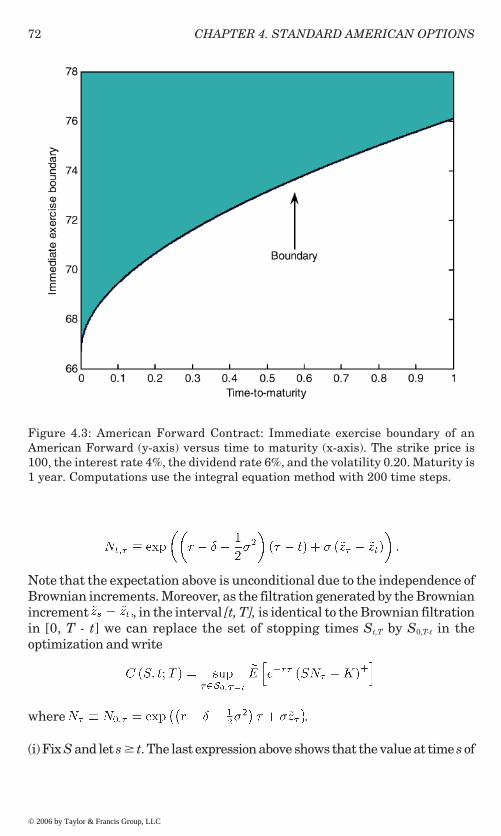
72 CHAPTER 4. STANDARD AMERICAN OPTIONS
Note that the expectation above is unconditional due to the independence ofBrownian increments. Moreover, as the filtration generated by the Brownianincrement , in the interval [t, T], is identical to the Brownian filtrationin [0, T - t] we can replace the set of stopping times St,T by S0,T-t in theoptimization and write
where .
(i) Fix S and let s � t. The last expression above shows that the value at time s of
Figure 4.3: American Forward Contract: Immediate exercise boundary of anAmerican Forward (y-axis) versus time to maturity (x-axis). The strike price is100, the interest rate 4%, the dividend rate 6%, and the volatility 0.20. Maturity is1 year. Computations use the integral equation method with 200 time steps.
© 2006 by Taylor & Francis Group, LLC

73
an option with maturity date T is the same as the value at t of an option withmaturity date T - s + t and same strike price, i.e., (this follows immediately from Furthermore, as
, we obtain Byassumption, immediate exercise is optimal at t. Thus Ifimmediate exercise is suboptimal at (S, s) we also have which contradicts the previous inequality.
(ii) Take S1 > S2 and suppose that (S2, t). ∈ ε while (S1, t). ∉ ε Let �1 be theoptimal stopping time at (S1, t). We have the following sequence of relations
The equality in the first line above results from the optimality of �1 at (S1,t). The inequality in the third line uses (a+b)+ � a++b+. The fourth linefollows from the suboptimality of �1 at (S2, t), the fifth from S1 - S2 > 0 andthe supermartingale property of S, and the last line from the assumptionthat immediate exercise at (S2, t) is optimal. Hence C (S1, t) � S1–K, whichcontradicts the assumption that immediate exercise is suboptimal at (S1,t). We conclude that (S1, t). ∈ ε. This corresponds to the property stated,with �≡S1/S2>1. The case � = 1 is trivial.
(iii) Suppose that 0 < S < K. As P[Sv > K] > 0, for some v ∈ [t, T), immediateexercise is a suboptimal policy. Suppose that K � S < (r/δ) K and assumethat immediate exercise is optimal, i.e., C(S, t) = S – K. Consider the portfolioconsisting of 1 call option, 1 share of the stock held short and K dollarsinvested at the riskfree rate. Define the stopping time
or � = T if no such time exists. Suppose that we liquidate this portfolio at �.The cash flows generated by this policy are
4.9. APPENDIX: PROOFS
© 2006 by Taylor & Francis Group, LLC

74 CHAPTER 4. STANDARD AMERICAN OPTIONS
Given that rK – δSv > 0 for all v < � we have constructed an arbitrageportfolio. As the existence of an equilibrium implies the absence of arbitrageopportunities it must be the case that C (S, t) > S - K, i.e., immediateexercise is a suboptimal policy.
(iv) Immediate exercise is optimal at the maturity date if and only if S �K.
Proof of Proposition 32:(i) This result can be proved by using the continuity of the option payoff
function and the continuity of the flow of the stochastic differential equation(4.1) relative to the initial values. Precise arguments can be found in Jaillet,Lamberton and Lapeyre [1990] (see their Proposition 2.2 and thecorresponding proof). Continuity with respect to the first argument, theunderlying asset price, also follows from the proof of property (iv) below.
(ii) Suppose S1 > S2 and define S� ≡ �S1+(1–�)S2. As the call option payoff isnon-decreasing and convex with respect to the asset price, we have, for any �∈ S0,T-t,
Taking present values and evaluating the payoffs at the optimal exercisepolicies associated with the two prices establishes that the option price isnon-decreasing and convex.
(iii) This is a straightforward counterpart of Proposition 31 (i).(iv) Consider (S1, t) and (S2, t) such that S1 > S2. For any stopping time t
� ∈ S0,T-t, we have
In particular this holds for the optimal stopping time �1 associated with(S1, t). Hence, we can write
where the last inequality follows because S1 - S2 > 0 and because thediscounted price of a dividend-paying asset is a Q-supermartingale.
© 2006 by Taylor & Francis Group, LLC
75
Dividing both sides by S1 – S2 proves the statement (this argument alsoestablishes the continuity of the option price with respect to S).
Proof of Proposition 33: Property (iii) of Proposition 32 implies that theboundary is non-increasing in time. This feature combined with thedefinition of the boundary implies that B(t-) � B(t) � B(t+) where B(t-) andB(t+) are the left and right limits of the boundary at t.
Suppose now that (S, v) ∈ ε for all v > t. As ε is a closed set we have Thus, In particular (take S
= B (t+) in the previous argument). As t+ = t, up-connectedness of the exerciseregion implies B(t+) � B(t). This combined with the reverse inequality (seeabove) establishes that B(t+) = B(t) (i.e., the exercise boundary is rightcontinuous).
Left continuity of the boundary can be proved using the arguments inJacka (1991) adapted to the call option case. Accordingly, suppose that B(t-)> B(t). Then there exists an open set B(t), B(t-))≡0 such that 0 � ε and forall x ∈ O there exists a sequence {xn} ∈ � with x = lims↑txn. Let us now usethe fact that the option price is C2,1 (R+×[0,T]) and satisfies the fundamentalPDE (see Merton [1973a], Jacka [1991] and Jaillet, Lamberton and Lapeyre[1990])
for all (S, t) ∈ C. Evaluating this equation along the sequence {xn} shows that,in the limit (at the point x = lims↑txn in the closure of the continuation region),
As B(t) � (r/δ) K we conclude that Css(x, t) � 0 for all x ∈ O and Css(x,t) � for x in a subset of O with positive Lebesgue measure. Integration
by parts now gives
By definition of ε the left-hand side of this expression is null. The righthand side, on the other hand, is no less than ε, for some ε > 0. Thiscontradiction implies that the set O must have null Lebesgue measure, inother words that
To show that BT– = max {K, (r/δ)Κ} note that property (iii) of Proposition31 gives the lower bound Suppose that BT– = max{K, (r/δ)Κ} and consider a point Then C(x, t)> x – K for all t ∈ [0, T). Thus, (in fact C(x,T–) � x – K + ε for some ε > 0 when x is sufficiently below BT-). But, by thecontinuity of the price function, we also have C(x, T-) = C(x, T) = x - K
4.9. APPENDIX: PROOFS
© 2006 by Taylor & Francis Group, LLC
� ���� � � ����

76 CHAPTER 4. STANDARD AMERICAN OPTIONS
(as x > K), a contradiction. We conclude that the interval (max {K, (r/δ )K},BT–) has null Lebesgue measure, i.e., that BT–= {K, (r/δ )K}.
To complete the proof we need to identify the boundary B–∞. This limitingvalue can be obtained from the EEP formula (4.2) in Theorem 34 taking T = ∞(see Corollary 35).
Proof of Theorem 34: Proposition 31 implies B � max{K, (r/δ) K}. Hence Y= (S - K)+ equals S - K in ε. It follows that in theexercise region, i.e., Theorem 21 thenimplies
Under the GBM assumption the expectation above can be computed explicitly.This leads to (4.2)–(4.3). The recursive equation for the optimal exerciseboundary is obtained by imposing the boundary condition C(B, t) = B - K.
Proof of Corollary 35: When T ↑ ∞ the immediate exercise boundarybecomes time independent: B = B∞. It follows that
and are independent ofB∞. As the European call option value converges to 0 the recursiveequation (4.6) becomes linear in B∞ and has the unique solution
The value of the option then follows from(4.2): the early exercise premium simplifies to
Proof of Proposition 36: The property is a special case of Theorem 26.
Proof of Theorem 37: In the exercise region the EEP representationstates Twice differentiating withrespect to S, and using the relation
gives
where
© 2006 by Taylor & Francis Group, LLC

77
and
Given that the exercise set is closed we can take the limit as S → Bt to obtain
and substituting
we can write
Solving for log(Bt) and using the definitions of I(Bt, B(.)) and J(Bt, B(.))establishes the statements in the theorem.
Proof of Proposition 38: Taking the derivative of (4.2) and simplifyingleads to the expression announced. Continuity follows from the continuityof h(St, t) and d(St, Bs, s - t) with respect to S, and the continuity of N(x) andn(x) with respect to their argument x. In the exercise region immediate
4.9. APPENDIX: PROOFS
© 2006 by Taylor & Francis Group, LLC
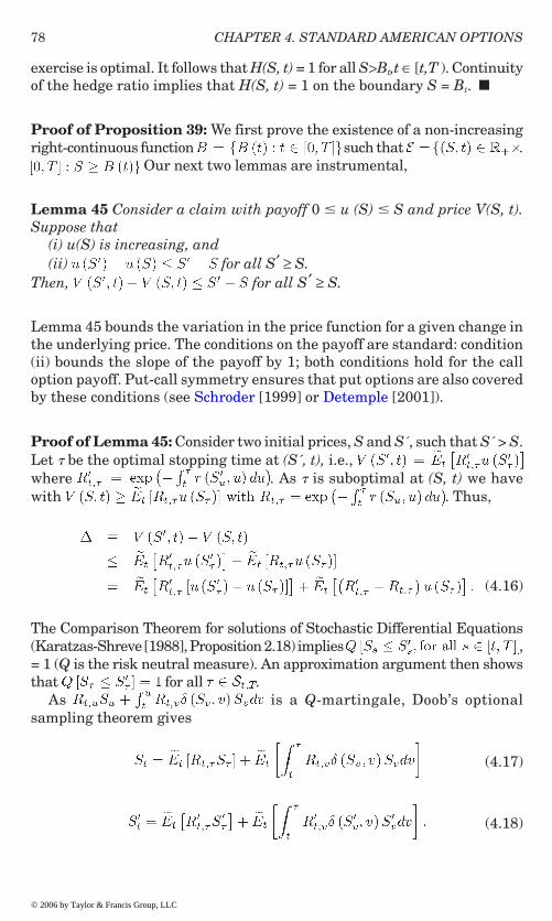
78 CHAPTER 4. STANDARD AMERICAN OPTIONS
exercise is optimal. It follows that H(S, t) = 1 for all S>Bt,t ∈ [t,T ). Continuityof the hedge ratio implies that H(S, t) = 1 on the boundary S = Bt.
Proof of Proposition 39: We first prove the existence of a non-increasingright-continuous function such that .
Our next two lemmas are instrumental,
Lemma 45 Consider a claim with payoff 0 � u (S) � S and price V(S, t).Suppose that
(i) u(S) is increasing, and(ii) for all S′ ≥ S.
Then, for all S′ ≥ S.
Lemma 45 bounds the variation in the price function for a given change inthe underlying price. The conditions on the payoff are standard: condition(ii) bounds the slope of the payoff by 1; both conditions hold for the calloption payoff. Put-call symmetry ensures that put options are also coveredby these conditions (see Schroder [1999] or Detemple [2001]).
Proof of Lemma 45: Consider two initial prices, S and S´, such that S´ > S.Let � be the optimal stopping time at (S´, t), i.e., where . As � is suboptimal at (S, t) we havewith . Thus,
(4.16)
The Comparison Theorem for solutions of Stochastic Differential Equations(Karatzas-Shreve [1988], Proposition 2.18) implies ,= 1 (Q is the risk neutral measure). An approximation argument then showsthat for all .
As is a Q-martingale, Doob’s optionalsampling theorem gives
(4.17)
(4.18)
© 2006 by Taylor & Francis Group, LLC
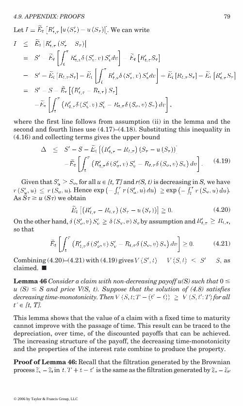
79
Let . We can write
where the first line follows from assumption (ii) in the lemma and thesecond and fourth lines use (4.17)–(4.18). Substituting this inequality in(4.16) and collecting terms gives the upper bound
(4.19)
Given that , for all u ∈ [t, T] and r(S, t) is decreasing in S, we have. Hence exp exp .
As S� � u (S�) we obtain
(4.20)
On the other hand, by assumption and ,so that
(4.21)
Combining (4.20)–(4.21) with (4.19) gives asclaimed.
Lemma 46 Consider a claim with non-decreasing payoff u(S) such that 0 �u (S) � S and price V(S, t). Suppose that the solution of (4.8) satisfiesdecreasing time-monotonicity. Then for allt´ ∈ [t, T].
This lemma shows that the value of a claim with a fixed time to maturitycannot improve with the passage of time. This result can be traced to thedepreciation, over time, of the discounted payoffs that can be achieved.The increasing structure of the payoff, the decreasing time-monotonicityand the properties of the interest rate combine to produce the property.
Proof of Lemma 46: Recall that the filtration generated by the Brownianprocess in is the same as the filtration generated by
4.9. APPENDIX: PROOFS
© 2006 by Taylor & Francis Group, LLC

80 CHAPTER 4. STANDARD AMERICAN OPTIONS
in [t´, T]. Let U ≡ T - t´ be the length of these time intervals and let denote the Brownian motion that carries the common
filtration. The set of stopping times of this filtration is With these definitions we can write
The expression after the first equality is the usual value of the Americanclaim where S(S,t) solves (4.8) subject to the initial condition St = S. To getthe second equality we use the fact that the Brownian motion generatesthe same filtration and is such that . The expectation is takenrelative to this Brownian motion and the corresponding measure . Theprocess solves
and the discount factor is
Let h = t´ - t. Similar steps show that
where solves the time-shifted equation
and
With these transformations the value functions become easy to compare.Decreasing time-monotonicity implies that for all
and, as the payoff is a non-decreasing function, we obtain for all The properties of the interest rate
(decreasing in the first argument and increasing in the second argument)also enable us to conclude that . The lemma follows.
Proof of Proposition 39 (continued): To show that the exercise region isup-connected note that the call payoff satisfies the conditions of Lemma45. Thus, Suppose then thatimmediate exercise is optimal at (S, t) but not at (S’, t). The optimality of
© 2006 by Taylor & Francis Group, LLC

81
exercise at (S, t), combined with the inequality above, implies This contradicts the suboptimality of
exercise at (S´, t). We conclude that immediate exercise must also be optimalat (S´, t). As this holds for any (S, t) ∈ ε the exercise region is up-connected.The existence of a unique exercise boundary follows.
To show that the boundary is non-increasing (i.e., that the exercise regionis right-connected) we proceed as follows. Suppose (S, t) ∈ ε and t́ > t. Wewant to show (S, t) ∈ ε. Suppose not, i.e., suppose that C (S,́ ; t) > (S–K )+. Inthis case we have
The inequality in the second line follows from Lemma 46. The last inequalityis the assumption that immediate exercise is suboptimal at t´. Given that(S, t) ∈ ε we have a contradiction.
The same arguments as in the proof of Proposition 33 can be used toprove the right continuity of the exercise boundary.
Proof of Proposition 40: The structure of the exercise set and the validityof the EEP representation follow from Proposition 39.
To establish (4.14)–(4.15) we pass to a new numeraire corresponding tothe detrended asset price. Substituting the underlying price in the strikefunction gives
and with
An application of Ito’s lemma shows that
Substituting in x and using the translated (under the risk neutral measure)Brownian motion gives
4.9. APPENDIX: PROOFS
© 2006 by Taylor & Francis Group, LLC

82 CHAPTER 4. STANDARD AMERICAN OPTIONS
Under the measure the process z* is a Brownianmotion (by Girsanov’s theorem). It follows that
where and z isa random variable with standard normal distribution function.
The European option value is
The two probability elements are respectively,
and
where
The pricing formula (4.14) follows from the relations exp and
For the early exercise premium note that, by Ito’s lemma,
© 2006 by Taylor & Francis Group, LLC

83
with . The EEP is given by
The first probability element is
The second one simplifies as follows,
where the integral in the last term equals .
Combining all these expressions produces the formulas in (4.15). Therecursive equation for the immediate exercise boundary is obtained usingstandard arguments. The boundary condition follows from the dividend
paid by Y as t → T.
Proof of Proposition 41: Properties (i) and (iii) are standard. For (ii)note that
for � � 1, where t stands for the optimal exercise time. A standard argumentcan now be applied to conclude that the claim holds.
Proof of Proposition 42: The arguments in Jaillet, Lamberton andLapeyre [1990], Proposition 2.2, can be invoked to prove the continuity in(i). Property (ii) is a consequence of the affine, increasing payoff structure.
4.9. APPENDIX: PROOFS
© 2006 by Taylor & Francis Group, LLC

84 CHAPTER 4. STANDARD AMERICAN OPTIONS
Property (iii) is the counterpart of (i) in Proposition 41. The proof of (iv) is anadaptation of the proof of (iv) in Proposition 32. �
Proof of Proposition 43: The proof parallels the proof of Proposition 33for call options. The only difference is the “exercise” boundary at maturity,equal to BT = 0. This value is implied by the obligatory nature of the contractat the expiration date. �
Proof of Proposition 44: An application of Theorem 21 to the payofffunction S - K leads to the formulas indicated. �
© 2006 by Taylor & Francis Group, LLC

Chapter 5
Barrier and CappedOptions
This chapter examines the valuation of American barrier and capped options.Barrier options, such as down-and-out calls, are considered first (section 5.1).The case of capped options is treated next (section 5.2). Contracts with constantand growing caps are analyzed in the Black-Scholes setting with constantcoefficients, of chapter 4. Results are also reported for capped options withstochastic caps, that are written on nondividend-paying assets with stochasticvolatility. Insights about the optimal exercise policy when the underlyingasset price follows a diffusion process are also provided (section 5.3).
5.1 Barrier Options
5.1.1 Definitions and Literature
A barrier option is an option whose payoff depends on whether the underlyingasset price reaches a pre-specified level, the barrier, during a certain timeperiod. The most common examples are knock-in and knock-out options. Aknock-in option comes into existence, while a knock-out option expires, whenthe barrier is reached. Knock-in and knock-out options each come in twovarieties (down and up) depending on the position of the barrier relative tothe initial asset price. If the barrier is below the underlying price at inception,the option is a down-and-in or a down-and-out option; if it lies above, theoption is an up-and-in or an up-and-out option. All these contracts exist inthe form of puts and calls. For instance, a down-and-in put is a put optionthat comes into existence when the underlying asset price decreases to a pre-specified barrier; a down-and-out call is a call option that expires when thebarrier is reached. Knock-out options can involve a payoff at expiration. Ifthey do, the payment is called a rebate.
Vanilla barrier options, such as those described above, are sometimes called“one touch” barrier options to emphasize the fact that an event materializes at
© 2006 by Taylor & Francis Group, LLC

CHAPTER 5. BARRIER AND CAPPED OPTIONS86
the first touch of the pre-specified barrier. This contractual provision can becontrasted with more exotic barrier and event specifications that have begunto appear in derivatives markets and that will be dealt with in chapter 7.
European-style barrier options have been studied by Cox and Rubinstein[1985], Rubinstein and Reiner [1991] and Boyle [1992]. Hedging aspects areaddressed by Bermin [2002], [2003]. American-style contracts are examinedby Gao, Huang and Subrahmanyam [2000].
5.1.2 ValuationOur analysis is carried out in the context of the Black-Scholes market setting.Consider an American down-and-out call option with maturity date T, exerciseprice K and barrier H with K > H. In the event that the barrier is reached ator before maturity the option payoff is null (the rebate is assumed to be null).On the complementary event the holder has the right to exercise the optionand collects (S - K)+ if he/she chooses to do so.
The down-and-out call option is a simple example of a path-dependent contractbecause the payoff depends on the trajectories followed by the underlying assetprice. In spite of this apparent complexity the valuation of this American-stylecontract is straightforward. It rests on a simple extension of the EEPrepresentation to American-style contracts with random maturity. Formulasof this type emerge in several valuation problems involving derivatives withtrigger levels (such as the capped options examined further in this chapter).
Theorem 47 (EEP representation) Consider an American down-and-outcall option with maturity date T, exercise price K and barrier K > H. LetBdoc be the optimal exercise boundary, Cdo(S, t, H, B doc (.)) the value of thecontract, and c do(S, t, H) the value of a down-and-out European call withidentical characteristics (T, K, H). For H < S < Bdoc and t ∈ [0, T], the valueof the American down-and-out call is given by
(5.1)
where
and denotes the first hitting time of H in [t,T], or if no such time exists in [t, T]. The optimal exercise boundarysolves the recursive integral equation
(5.2)
subject to the boundary condition .
© 2006 by Taylor & Francis Group, LLC

87
This decomposition of the American down-and-out call option is similar tothe early exercise premium representation for standard American options(Theorem 34). The first component is the European down-and-out call price.The second component, the early exercise premium, again represents thepresent value of the benefits from early exercise. For the contract underconsideration the benefits are collected as long as the contract is alive, i.e., aslong as the underlying asset price exceeds the barrier H. When the barrier isattained (on the event {�H ≤ T}) the option is retired and loses all value.
As usual, the EEP representation (5.1) leads to an equation for the exerciseboundary (see (5.2)). The intuition here is standard. As immediate exercise isoptimal on the boundary the value given by (5.1) must equal the exercisepayoff when both are evaluated at S = Bdoc.
The components of the EEP representation can be expressed in more explicitform by taking advantage of the availability of a closed form solution for thejoint distribution of the asset price and the hitting time �H.
Corollary 48 The EEP components of the American down-and-out calloption value are
(5.3)
and
(5.4)
where
and In (5.3) terms in d±(x) are evaluated at v = T.
For the up-and-out put similar computations can be performed to obtain
Theorem 49 (EEP representation) Consider an American up-and-out putoption with maturity date T, exercise price K and barrier K < H. Let B uop bethe optimal exercise boundary, Puo (S, t, H, Buop (.)) the value of the contract,
5.1 BARRIER OPTIONS
© 2006 by Taylor & Francis Group, LLC
.

CHAPTER 5. BARRIER AND CAPPED OPTIONS88
and puo (S, t, H) the value of an up-and-out European put with identicalcharacteristics (T, K, H). For H > S > Buop and t ∈ [0, T], the value of theAmerican up-and-out put is given by
(5.5)
where the European up-and-out put and the early exercise premium aregiven by
The optimal exercise boundary solves the recursive integral equation
(5.6)
subject to the boundary condition .
Inspection of the formulas for the down-and-out call and the up-and-out putreveals the following relationship
Proposition 50 (American barrier option put-call symmetry) Consider anAmerican up-and-out put option with characteristics (T, K, H), written onan asset whose price satisfies (4.1). The symmetry relation Puo(S, K, H, r, δ,T) = Cdo(K, S, KS/H, δ, r, T) holds. The exercise boundaries are related byBuop = SK/B doc.
This proposition extends the put-call symmetry property for standardAmerican options (Theorem 3.13) to the case of barrier options. An importantdifference, relative to plain vanilla contracts, is that the barrier must also beadjusted when passing from the put to the call. The exercise boundaries onthe other hand stand in the usual relationship. This result, that can beproved by using the change of numeraire outlined in section 2.7 (i.e., passingto the equivalent probability measure Q* in (2.23)), is a special case of thegeneral put-call symmetry for random maturity options (see Section 4 inDetemple [2001]).
© 2006 by Taylor & Francis Group, LLC

89
5.2 Capped Options
5.2.1 Definitions, Examples and Literature
A capped option is a contract whose payoff is limited by some pre-specifiedamount. For example a capped call option with cap L and strike K pays off
upon exercise; a capped put option with cap L and strike Kpays off Capped options can be European- or American-style.They can also incorporate automatic exercise provisions. For example, a cappedcall option with maturity date T and automatic exercise at the cap is a callwith random maturity given by the first time at which the underlying assetprice reaches the cap, or the maturity date if no such time exists prior to T.This contract is a knock-out barrier option with rebate equal to the optionpayoff at the trigger date. Finally, the cap provision can be a constant, afunction of time, or a stochastic process. Examples of capped options withtime-dependent caps include contracts with discrete monitoring dates.
Several contracts with cap provisions have been issued by firms or financialinstitutions in the last two decades. One example is the MILES contract(Mexican Index-Linked Euro Security). This security is a package comprisedof several securities including an American call option on the dollar value ofthe Mexican stock index. The contract is unusual in that it has both a time-dependent cap and a restriction on the exercise period.
Other examples are the capped options on the S&P 100 and S&P 500 indicesthat were introduced by the Chicago Board of Options Exchange (CBOE) inNovember 1991. These capped index options, which are called CAPS, combine aEuropean exercise feature (the holder of the security cannot choose to exerciseuntil the maturity of the contract) with an automatic exercise provision. Theautomatic exercise provision is triggered if the index value exceeds the cap at the
Additional examples of European capped options include the range forward contract,collar loans, barrier options, indexed notes and index currency option notes (see
European capped options are studied by Boyle and Turnbull [1989].American-style contracts are examined by Broadie and Detemple [1995],[1997a], [1999] in the Black-Scholes setting and Detemple and Tian [2002] ina more general class of diffusion models.
5.2.2 Constant CapIn this section and the next we suppose that the market satisfies the Black-Scholes assumptions (model with constant coefficients) with positive interestrate. In this setting consider an American capped call option with maturitydate T, exercise price K and constant cap L with L > K. Upon exercise the
1 The call payoff is capped by L - K; for the put option the maximum payoff is K - L. Theconstant L corresponds to the cap on the underlying asset price.
5.2 CAPPED OPTIONS
© 2006 by Taylor & Francis Group, LLC
close of any trading day (see Flesaker [1992] for a critical analysis of these options).
Boyle and Turnbull [1989] and Rubinstein and Reiner [1991] for details).

CHAPTER 5. BARRIER AND CAPPED OPTIONS90
contract pays . Let BL and CL(S, t) denote the optimal exerciseboundary and the price of the capped option, respectively. The optimal exerciseboundary is characterized in Theorem 51 and illustrated in Figure 5.1
Theorem 51 Consider an American-style capped call option with maturitydate T, exercise price K and constant cap equal to L with L > K. The optimalexercise boundary BL is given by
where B denotes the optimal exercise boundary of an American uncappedcall option with same maturity date and exercise price.
Figure 5.1: GBM model. Exercise boundary of a capped call option (y-axis) versustime to maturity (x-axis). The strike price is 100, the cap 160, the interest rate 6%and the dividend rate 4%. Computations use the integral equation method with2,000 time steps.
© 2006 by Taylor & Francis Group, LLC
0 0.1 0.2 0.3 0.4 0.5 0.6 0.7 0.8 0.9 1150
155
160
165
170
175
180
Time-to-maturity
Imm
edia
te e
xerc
ise
boun
dary
B
LT-t*

91
The exercise boundary of the capped call option has a very simple structureindeed! Intuition for this result can be gathered by examining the variousconfigurations of the asset price S, the cap L and the exercise boundary Bthat can materialize. When S is above the cap waiting to exercise is suboptimaldue to the time value of money. When S is below the cap and the holder of the capped option can implement the optimal exercise policyand match the payoff of the uncapped American option with identical strikeand maturity date (see Figure 5.1). This policy will therefore be optimal forthe capped option as well. From these two observations one concludes thatthe exercise boundary for the capped option BL is always bounded above byB�L and is equal to B at the first time t* at which B (t) = L. When S liesbelow the cap and (i.e., before t*) the argument is more subtle.In this situation it can be shown that the holder of the capped option can infact duplicate the optimal exercise policy and the payoff of an uncapped optionwith shorter time-to-maturity for which immediate exercise is suboptimal(see the proof in the Appendix).
With the optimal exercise policy fully identified, the valuation of the contractbecomes easy to perform. Let t* be the solution of the equation
if an interior solution, with value in [0, T], exists. If B (t, T) < L for all t ∈ [0,T] set t* = 0. If B (t, T) > L for all t ∈ [0, T] set t* = T. The next theoremprovides a valuation formula for the American capped call option.
Theorem 52 Consider an American-style capped call option with maturitydate T, exercise price K and constant cap equal to L (L > K). For the option value is
given by
(5.7)
where denotes the first hitting time of L in [t,T] and if no such time exists in [t, T]. The representation formula in(5.7) can be simplified by computing the expectations explicitly
(5.8)
where
(5.9)
(5.10)
5.2 CAPPED OPTIONS
© 2006 by Taylor & Francis Group, LLC

CHAPTER 5. BARRIER AND CAPPED OPTIONS92
(5.11)
An alternative decomposition that draws on Theorems 51 and 52 relatesthe value of the American capped option to the value of a capped option withautomatic exercise at the cap.
Theorem 53 (Early exercise premium representation) Let Cae (S, t, L) bethe value of a capped option with automatic exercise at the cap (see formula(5.13) below). For the value of the American capped
option is given by
(5.12)
where denotes the first hitting time of L in [t,T], and if no such time exists in [t, T].
This decomposition of the American option value is similar to the early exercisepremium representation for standard American options (Theorem 34). It differs inthat it relates the value of the option contract to the value of a contract that maybe automatically exercised before the maturity date (the standard representationuses the value of a European option with exercise at the maturity date as thebenchmark). This is the first component on the right hand side of (5.12): a callwith automatic exercise at the cap. The second component in (5.12) measures thepremium achieved by optimally exercising prior to reaching the cap. The premiumis the present value of net benefits in the event of exercise, consisting of the dividendscollected on the underlying asset net of the interest costs incurred.
When dividends are sufficiently low the exercise boundary of the uncappedoption B exceeds the cap L at all times. In this case the valuation formulas(5.7) and (5.12) simplify significantly. Straightforward deductions show that,
Corollary 54 (American capped call valuation with low dividends) Supposethat the value of the American cappedcall option equals the value of the corresponding capped call option withautomatic exercise at the cap
(5.13)
© 2006 by Taylor & Francis Group, LLC

93
In (5.13) the expressions for d0 and are the same as in (5.10)–(5.11) butwith � = T - t replacing t* - t. The expressions for b,f, φ, and α are the sameas in Theorem 52.
Remark 5 The value of a European capped call option with strike price K,cap L and maturity T (the option with payoff isgiven by
The European capped option value can serve as a benchmark to measurethe gains from early exercise (prior to maturity) embedded in the Americancapped option value. The early exercise premium is particularly simple tocompute in the case of low dividends (formula (5.13)).
Remark 6 If L ↑ ∞ the European capped call option value C e (S, t, L) convergesto the Black-Scholes formula adjusted for dividends (see corollary 15).
5.2.3 Capped Options with Growing CapsConsider now the class of American capped options whose caps grow at aconstant rate g ≥ 0. Suppose that
(5.14)
where we assume that L0 > K. Let t* denote the solution to the equation B (t,T) = Lt, if an interior solution in [0, T] exists. If B (t, T) < Lt for all t ∈ [0, T]set t* = 0. If B (t, T) > Lt for all t ∈ [0, T] set t* = T . In order to describe theoptimal exercise region it is necessary to consider the class of exercise policiesdefined next and illustrated in Figure 5.2.
Definition 55 ( Exercise Policy). Let te and t
f satisfy
and Define the stopping times
An exercise policy is a (te, t*, t f)-policy if the option is exercised at the stoppingtime
A (te, t*, t f)-policy is an exercise policy that is completely described by thethree parameters indicated. Moreover, one of the parameters (t*) is alreadydetermined as the solution to an equation, while the other two (te and tf) arearbitrary constants, up to the restrictions
5.2 CAPPED OPTIONS
© 2006 by Taylor & Francis Group, LLC

CHAPTER 5. BARRIER AND CAPPED OPTIONS94
A (te, t*, t f)-policy mandates immediate exercise along the cap if the time-to-maturity is less than T - te. In the interval [0, T - t* ] exercise is immediate ifthe underlying asset price lies in between the exercise boundary B and thecap L. For times-to-maturity less than T - t f immediate exercise is alsoimplemented if the asset price lies above the cap.
Our first theorem identifies the optimal exercise policy.
Theorem 56 Consider an American capped call option with exercise priceK, maturity date T and cap given by equation (5.14). Then the optimalexercise policy is a (t
e, t* , t
f)-policy.
This result is quite surprising because it shows that the optimal stoppingtime belongs to the class of (te, t*, t f)-policies introduced in definition 55. Aswe shall see shortly, the parameter tf (in addition to t*) is already determinedby the structure of the capped option payoff, the cap process, the underlying
Figure 5.2: A (te t*, t
f)-policy for a capped call option with growing cap. Time-to-
maturity is on the x-axis: point e corresponds to T - te, point f is T - t
f. The option
strike is K = 100, the initial cap L0 = 200, the cap’s growth rate is g = 10%, theinterest rate r = 6%, the dividend rate δ = 3% and the volatility coefficient σ = 0.2.Computations use the integral equation with 2000 time steps.
© 2006 by Taylor & Francis Group, LLC

95
asset price process and the interest rate. So is the only parameterthat remains to be determined: pricing the American capped call option hasbeen reduced to the identification of a single parameter, te. This boils down toa univariate optimization problem that can be resolved by using the valuationformula given in Theorem 57 below.
Intuition for the optimality of a (te, t*, tf)-policy is as follows. First, note thatimmediate exercise is optimal for the capped option in the region B < S < Lbecause it is optimal for the uncapped option and the payoffs are identical.Similarly, when t ≥t* and S < B (t) the capped option holder can implementthe exercise policy of the uncapped option and collect the same payoff. Second,note that immediate exercise is also optimal if t ≥ tf and S > Lt. In this regionthe discounted payoff decreases almost surely and, as a result, waiting reducesvalue. The reverse argument applies when t < tf and S > Lt. Here the discountedpayoff t increases over time which means that the policy ofexercising at where tL is the first hitting time of the cap L, increasesvalue. Third, when t < t* and S < Lt one can find an uncapped option withshorter time-to-maturity whose exercise boundary falls below the cap at allsubsequent times. Implementation of this exercise policy dominates immediateexercise for the capped option holder. Lastly, along the cap (i.e., when S = Land t < t*) the benefits of waiting (which dominate above the cap) are curtailedby the risk of falling below the cap. When the maturity date is sufficientlyclose (i.e., for t close to t*) this risk is enough to prompt immediate exercise.With longer horizons the appreciation in the discounted value of the cap can besufficient for the optimality of a waiting policy.
The value of a (te, t*, tf)-policy is easy to calculate. The price of the American-style capped contract naturally follows.
Theorem 57 (Valuation of American capped option with growing cap) Define
The value of the American capped option with growing cap is given by
(5.15)
where
(5.16)
and C u and C d are the values at time t e in the events , respectively. Explicit formulas for Cu and C d are given in Broadie and
Detemple [1995].
Consider a fixed parameter te along with the parameters t* and tf definedabove. The value of the (te, t*, t f)-policy is given by CL (te, t*, t f) in formula(5.16). It follows immediately that the value of the American-style cappedoption is obtained by maximizing this value relative to the free parameter te.Even though this optimization problem does not have a simple closed formsolution it can be resolved numerically, by using standard methods.
5.2 CAPPED OPTIONS
© 2006 by Taylor & Francis Group, LLC

CHAPTER 5. BARRIER AND CAPPED OPTIONS96
5.2.4 Stochastic Cap, Interest Rate and VolatilityThis section considers a fairly general class of American capped optionswritten on nondividend-paying assets in a setting with stochastic interestrate and stochastic return volatility. The asset price S satisfies (under the Q-measure)
(5.17)
where volatility follows a stochastic process that isprogressively measurable, bounded above and bounded away from zero (P-a.s.) and the interest rate is progressively measurable,strictly positive and bounded.
The capped call option has payoff , where L satisfies
(5.18)
We assume that the growth rate of the cap, g, is a progressively measurableprocess such that Lt > K for all t ∈ [0, T] and such that the following growthcondition holds,
(5.19)
The model (5.17)–(5.19) for the underlying asset price and for the cap is fairlygeneral. It allows for a stochastic return volatility, a stochastic interest rateas well as a stochastic growth rate for the cap. The factor underlying thestochastic behavior of these quantities is the same Brownian motion thataffects the asset price: the market is complete. The cap’s growth rate maytake positive as well as negative values as long as condition (5.19) is satisfied.This condition is a restriction on the growth rate of the cap that is clearlysatisfied if the cap is constant or decreasing. It is satisfied even when thegrowth rate of the cap is positive as long as it is not too large. Broadie andDetemple [1999] consider the special case with constant interest rate.
For this model the following result holds,
Theorem 58 Consider an American capped call option with stochastic capgiven by (5.18)–(5.19) when the interest rate is a positive, bounded andprogressively measurable process, and the underlying asset price satisfies(5.17). The optimal exercise boundary is a stochastic process given by BL =L. If S ≥ L immediate exercise is optimal and CL (S, t) ≥ L - K. If S < L theoptimal exercise policy is described by the stopping time
�L≡ T if no such time exists. For S <
L and for all t ∈ [0, T], the value of the capped option is
(5.20)
© 2006 by Taylor & Francis Group, LLC
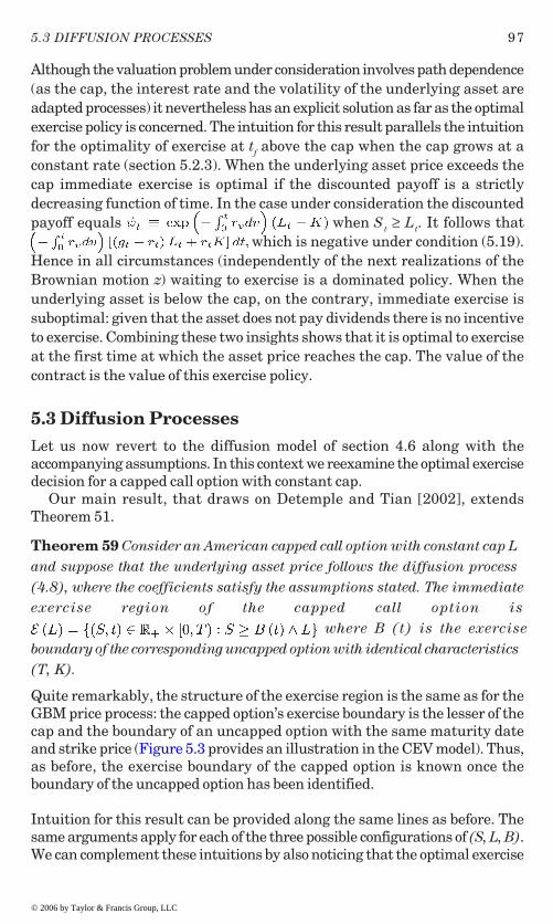
97
Although the valuation problem under consideration involves path dependence(as the cap, the interest rate and the volatility of the underlying asset areadapted processes) it nevertheless has an explicit solution as far as the optimalexercise policy is concerned. The intuition for this result parallels the intuitionfor the optimality of exercise at tf above the cap when the cap grows at aconstant rate (section 5.2.3). When the underlying asset price exceeds thecap immediate exercise is optimal if the discounted payoff is a strictlydecreasing function of time. In the case under consideration the discountedpayoff equals when S t ≥ Lt. It follows that
which is negative under condition (5.19).Hence in all circumstances (independently of the next realizations of theBrownian motion z) waiting to exercise is a dominated policy. When theunderlying asset is below the cap, on the contrary, immediate exercise issuboptimal: given that the asset does not pay dividends there is no incentiveto exercise. Combining these two insights shows that it is optimal to exerciseat the first time at which the asset price reaches the cap. The value of thecontract is the value of this exercise policy.
5.3 Diffusion ProcessesLet us now revert to the diffusion model of section 4.6 along with theaccompanying assumptions. In this context we reexamine the optimal exercisedecision for a capped call option with constant cap.
Our main result, that draws on Detemple and Tian [2002], extendsTheorem 51.
Theorem 59 Consider an American capped call option with constant cap Land suppose that the underlying asset price follows the diffusion process(4.8), where the coefficients satisfy the assumptions stated. The immediateexercise region of the capped call option is
where B (t) is the exerciseboundary of the corresponding uncapped option with identical characteristics(T, K).
Quite remarkably, the structure of the exercise region is the same as for theGBM price process: the capped option’s exercise boundary is the lesser of thecap and the boundary of an uncapped option with the same maturity dateand strike price (Figure 5.3 provides an illustration in the CEV model). Thus,as before, the exercise boundary of the capped option is known once theboundary of the uncapped option has been identified.
Intuition for this result can be provided along the same lines as before. Thesame arguments apply for each of the three possible configurations of (S, L, B).We can complement these intuitions by also noticing that the optimal exercise
5.3 DIFFUSION PROCESSES
© 2006 by Taylor & Francis Group, LLC
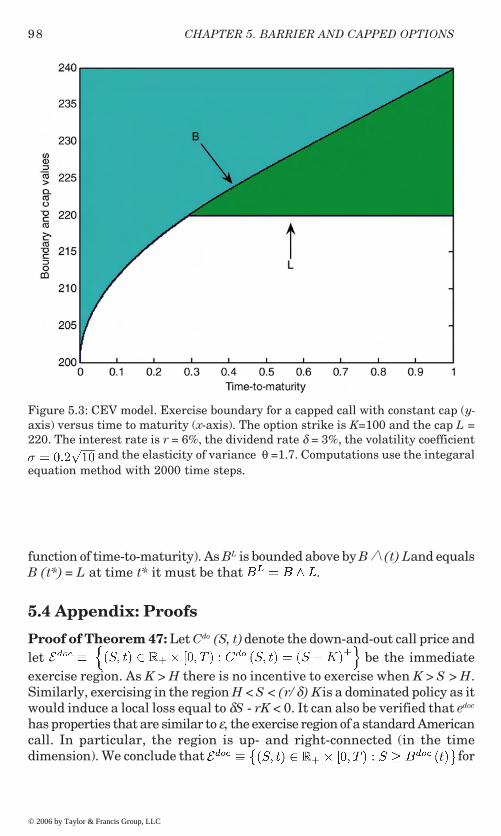
CHAPTER 5. BARRIER AND CAPPED OPTIONS98
function of time-to-maturity). As BL is bounded above by B � (t) L and equalsB (t*) = L at time t* it must be that .
5.4 Appendix: Proofs
Proof of Theorem 47: Let Cdo (S, t) denote the down-and-out call price andlet be the immediateexercise region. As K > H there is no incentive to exercise when K > S > H.Similarly, exercising in the region H < S < (r/ δ) K is a dominated policy as itwould induce a local loss equal to δS - rK < 0. It can also be verified that edoc
has properties that are similar to ε, the exercise region of a standard Americancall. In particular, the region is up- and right-connected (in the timedimension). We conclude that for
Figure 5.3: CEV model. Exercise boundary for a capped call with constant cap (y-axis) versus time to maturity (x-axis). The option strike is K=100 and the cap L =220. The interest rate is r = 6%, the dividend rate δ = 3%, the volatility coefficient
and the elasticity of variance θ =1.7. Computations use the integaralequation method with 2000 time steps.
© 2006 by Taylor & Francis Group, LLC

99
some non-increasing function of time Bdoc(.) . The function B
doc is the immediate
exercise boundary. It is continuous and converges to K as t → T.As the down-and-out call expires at the first hitting time �H of the level H
and as the payoff (S�H - K)+ = 0, the contract can be viewed as an American
option with random maturity �H. The early exercise premium representation
follows by a straightforward extension of the results in chapter 3. On theevent {�H = T } the payoff . On thecomplementary event . The formula in thetheorem follows.
The recursive integral equation for the boundary (5.2) is obtained from(5.1) using the fact that immediate exercise is optimal at the boundary, i.e.,at S = Bdoc. �
In order to demonstrate Corollaries 48, 54 and Theorem 49 we need theauxiliary lemmas stated below. These lemmas describe distributions andtruncated moment generating functions involving the first passage times ofsets with exponential boundaries, when the asset price follows a geometricBrownian motion process. The formulas provided can be inferred from the
Lemma 60 Suppose that S satisfies the stochastic differential equation dS=. For A = B define the conditional
probability,
Then
5.4 APPENDIX: PROOFS
© 2006 by Taylor & Francis Group, LLC
joint law of a Brownian motion and its running maximum (see Karatzas andShreve [1988], p. 95).

CHAPTER 5. BARRIER AND CAPPED OPTIONS100
Lemma 61 Suppose that L t =L0egt and that �L represents the first time in
[t, T] at which S=L (the first passage time of the level L). Then, for t ∈ [0, T],the conditional probability is given by
where
and.
Lemma 62 The conditional density of the first passage time tL is, for y ³ t,
Lemma 63 The truncated conditional moment generating function of �L is(at date 0)
where
Proof of Corollary 48: Using lemma 60 and a change of variable leads to
for A ≥ B. The European option value is
where is the conditional density of the distribution above.Performing the integration gives the expression for the European down-and-outcall. A similar computation produces the value of the early exercise premium. �
© 2006 by Taylor & Francis Group, LLC
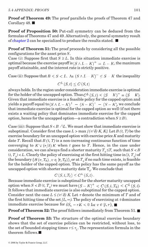
101
Proof of Theorem 49: The proof parallels the proofs of Theorem 47 andCorollary 48. �
Proof of Proposition 50: Put-call symmetry can be deduced from theformulas of Theorems 47 and 49. Alternatively, the general symmetry resultof chapter 2 can be specialized to produce the results stated. �
Proof of Theorem 51: The proof proceeds by considering all the possibleconfigurations for the asset price S .Case (i): Suppose first that S ≥ L. In this situation immediate exercise isoptimal because the exercise payoff is , the maximumpayoff attainable, and the interest rate is strictly positive.
Case (ii): Suppose that the inequality
always holds. In the region under consideration immediate exercise is optimalfor the holder of the uncapped option. Thus .Given that immediate exercise is a feasible policy for the capped option andyields a payoff equal to , we concludethat immediate exercise is optimal for the capped option as well (if not thereexists a waiting policy that dominates immediate exercise for the cappedoption, hence for the uncapped option—a contradiction when S ≥ B).
Case (iii): Suppose that S < B �L. We must show that immediate exercise issuboptimal. Consider first the case L > max {(r/δ) K, K}. Let B (t, T) be theexercise boundary for an uncapped option with exercise price K and maturitydate T. Recall that B (t, T) is a non-increasing continuous function of timeconverging to when t goes to T. Hence, in the case underconsideration, we can always find a shorter maturity T0 ≤T, such that S < B(t, T0) < L. Clearly the policy of exercising at the first hitting time in [t, T0) ofthe boundary or at T0 if no such time exists, is feasiblefor the holder of the capped option. This policy has the same payoff as theuncapped option with shorter maturity date T0. We conclude that
Because immediate exercise is suboptimal for the shorter maturity uncappedoption when S < B (t, T0) we must have .It follows that immediate exercise is also suboptimal for the capped option.Consider next the case L ≤ (r/ δ) K. Let � denote the minimum of T and ofthe first hitting time of the set [L, ∞). The policy of exercising at τ dominatesimmediate exercise because for ). �
Proof of Theorem 52: The proof follows immediately from Theorem 51. �
Proof of Theorem 53: The structure of the optimal exercise boundaryshows that the set of exercise policies can be restricted, without loss, tothe set of bounded stopping times � ≤ �
L. The representation formula in the
theorem follows.�
5.4 APPENDIX: PROOFS
© 2006 by Taylor & Francis Group, LLC

CHAPTER 5. BARRIER AND CAPPED OPTIONS102
bounded stopping times � ≤ �L. The representation formula in the theorem
follows.�
Proof of Corollary 54: When δ = rK/L the immediate exercise boundary isgiven by the cap L. The formula follows from the previous theorem.�
Proof of Theorem 56: The following cases arise.Case (i): Suppose first that B ≤ S < L. Then the same argument as in theproof of Theorem 51, case (ii) applies and demonstrates that immediate exerciseis an optimal policy.
Case (ii): Consider now the case S<B�Land suppose that (r/ δ) K > K. If Lt≥ (r/
δ) K the argument in the proof of Theorem 51, case (iii) applies. If Lt < (r/ δ) K the
policy of exercising at the stopping time � equal to the first hitting time of the set or T if no such time exists dominates immediate exercise because
). In the case (r/ δ) K ≤ K we have Lt > K for all t ∈ [0,
T] (by assumption) and the argument of Theorem 51, case (iii), again applies.
Case (iii): Suppose now that S > L. It can be verified that the discountedpayoff function has a unique maximum at
If tf is in the interior of [0, T] the function �t is strictly increasing for t < tf
and strictly decreasing for t > tf. If tf = 0 the discounted payoff �t is strictlydecreasing for t > tf; if tf = T it is strictly increasing for t < tf. Hence, if t = tf
immediate exercise dominates any waiting policy If t < tf the policy ofexercising at the first hitting time of L or at tf dominates immediate exercise.
Case (iv): Finally, suppose that immediate exercise is optimal at some time t< t* when S = L. Then it is optimal to exercise at all v ∈ [t, t*] when Sv = Lv.Suppose not, i.e., suppose that there exists u ∈ [t, t*] such that Su = Lu and
(for clarity we indicate the maturity dates of the optionsunder consideration). At t we have
(See Figure 5.4 for an illustration of L and its translation H.) If immediateexercise is suboptimal at u then (recall that Su = Lu)so that , a contradiction. We concludethat immediate exercise is optimal along the cap, for all v ∈ [t, t*], if it isoptimal at time t (i.e., the exercise region is a connected segment along thecap). �
© 2006 by Taylor & Francis Group, LLC

103
Lemma 64 Suppose that the underlying asset price S satisfies (4.1). Considertwo American capped call options written on S, with common maturitydate T and ex ercise price K, and respective caps L and H satisfying (5.14)withinitial condition L0 > H0.
Proof of Lemma 64: For any stopping time � ∈ S 0,T we have
where N0,� is the exponential process defined in the proof of proposition 31. As and the expression on the last line is,
Figure 5.4: Boundary and cap (y-axis) versus time to maturity (x-axis). The exerciseboundary of an uncapped call B, the cap function L and its translation H are plottedagainst time to maturity. The option strike is K = 100, the initial cap L0 = 150 andthe maturity date T = 1. The interest rate is r = 6%, the dividend rate δ = 4% and thevolatility coefficient σ = 0.2. Computations use the integral equation method with100 time steps.
5.4 APPENDIX: PROOFS
© 2006 by Taylor & Francis Group, LLC
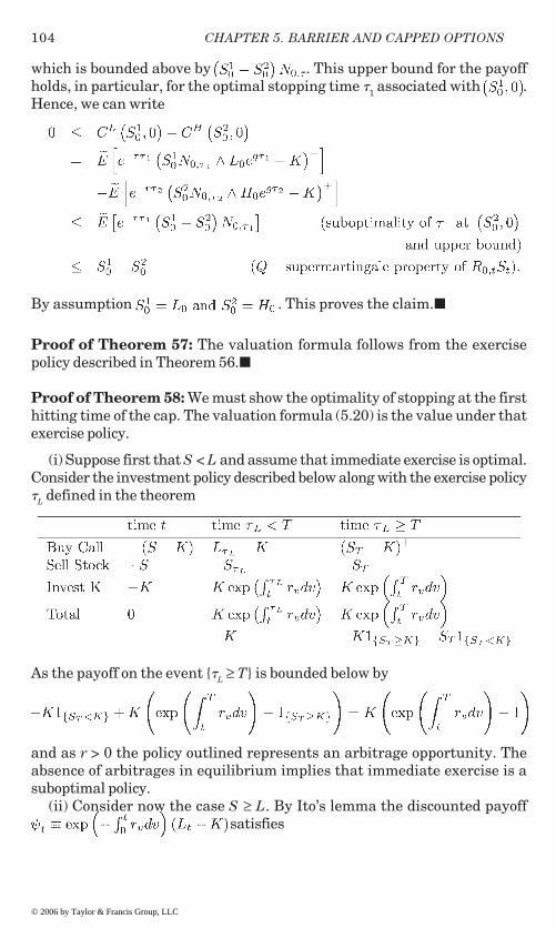
CHAPTER 5. BARRIER AND CAPPED OPTIONS104
which is bounded above by . This upper bound for the payoffholds, in particular, for the optimal stopping time �1 associated with .Hence, we can write
By assumption . This proves the claim.�
Proof of Theorem 57: The valuation formula follows from the exercisepolicy described in Theorem 56.�
Proof of Theorem 58: We must show the optimality of stopping at the firsthitting time of the cap. The valuation formula (5.20) is the value under thatexercise policy.
(i) Suppose first that S < L and assume that immediate exercise is optimal.Consider the investment policy described below along with the exercise policy�L defined in the theorem
As the payoff on the event {�L ≥ T} is bounded below by
and as r > 0 the policy outlined represents an arbitrage opportunity. Theabsence of arbitrages in equilibrium implies that immediate exercise is asuboptimal policy.
(ii) Consider now the case S ≥ L. By Ito’s lemma the discounted payoff satisfies
© 2006 by Taylor & Francis Group, LLC

105
Condition (5.19) implies that the process � is decreasing (P-a.s.). The optimalityof immediate exercise follows as any waiting policy leads to a decrease in thediscounted payoff. �
Proof of Theorem 59: Let t* be the smallest solution of the equation B (t) =L; or t* = T if L ≤ B (T); or t* = 0 if L ≥ B (0). If the boundary is only right-continuous and the cap passes in between two limit points, i.e., L ∈ [B(t), inf{B
s : s < t}], at some discontinuity point t, let t* be this unique point t.By the same arguments as in the proof of Theorem 51 we conclude that
, with equality for t ∈ [t*, T) (i.e., BL (t) = B (t) for t ∈ [t*,
T)). To show that the upper bound is attained for t ∈ [0, t*) we will use thefact that the function t → BL (t) is non-increasing. Define the difference
for t ∈ [t*, T). These properties combined with BL (t) non-increasing and Lconstant imply that Λ (t) for t ∈ [0, t*). �
5.4 APPENDIX: PROOFS
© 2006 by Taylor & Francis Group, LLC
107
Chapter 6
Options on Multiple Assets
This chapter is devoted to American options written on multiple underlyingassets. We first provide background information about multiasset options(section 6.1) and describe the financial environment (section 6.2). We thenstudy, in succession, options on the maximum of two assets (section 6.3),spread options (section 6.4), options on the average of two assets (section6.5) and options on the minimum of two assets (section 6.6). For each ofthese contracts the optimal exercise region is characterized and valuationformulas are provided. Extensions to derivatives on n > 2 assets arepresented in Appendix A.
6.1 Definitions, Examples and LiteratureAn increasing number of contractual rewards and obligations, held byeconomic entities, involve options that are written on multiple underlyingassets. Some of the payoffs that have become fairly common include optionson the maximum of several asset prices (max-options), options on theminimum of several prices (min-options), options on the difference betweentwo prices (spread options) and options on an average of prices (portfoliooptions). Contingent claims with these characteristics can be found onfinancial exchanges, in over-the-counter transactions, in cash flowsgenerated by investment decisions of firms and in executive compensationplans.
The simplest example of a multiasset contingent claim is an index option.A contract of this type is typically written on a portfolio of exchange-tradedassets and has an exercise payoff depending on an average of prices. Forinstance, S&P 100 Index Options, that have traded on the CBOE sinceMarch 1983, are American-style options written on the Standard & Poor’s100 Index, a capitalization-weighted index of 100 stocks. S&P 100 IndexLEAPS (Long-term Equity AnticiPation Securities) are long-datedAmerican-style options, on the same index. Options on the differencebetween asset prices, spread options, can also be found on severalexchanges. Crack Spread Options, traded on the New York MercantileExchange (NYMEX), are essentially contracts on the difference between rawmaterial and finished product prices. The Gasoline Crack Spread Option iswritten on the spread between the NYMEX New York Harbor unleaded gasoline
© 2006 by Taylor & Francis Group, LLC

CHAPTER 6. OPTIONS ON MULTIPLE ASSETS108
futures price and the NYMEX crude oil futures price. The Heating Oil CrackSpread Option is on the spread between the NYMEX New York Harbor heatingoil futures price and the NYMEX crude oil futures price. Both contracts areAmerican-style.
Derivatives paying the maximum or minimum of several prices or thedifference between two prices appear in a variety of contexts, often outsidethe realm of exchanges. Corporate bonds and managerial contractscommonly include ‘sweeteners’, taking the form of multiasset payoffs,designed to enhance the attractiveness of an issue or to provide adequateincentives. Embedded American max-options are routinely found in capitalbudgeting decisions confronting firms. They are typically associated withassets that can be put to multiple, but exclusive, uses. Real estatedevelopment companies, for instance, often face a choice among severalexclusive alternatives regarding land use. A particular type of spread options,options to exchange one asset for another, is also common. It characterizescertain employment switching decisions and is the hallmark of stock tenderoffers. Switching options are also standard in capital budgeting decisions.
In most cases the assets underlying these claims pay dividends orproduce cash flows. As shown in chapters 3 and 4, it is optimal to exercisean American-style claim written on a single dividend-paying asset, underappropriate circumstances. Intuition suggests that the same ought to betrue for multiasset claims. Clearly, if the local gains are large enough,early exercise will be optimal when the right conditions prevail. Thedetermination of these conditions, however, is not as straightforward asin the single asset case. The presence of multiple prices, that jointlydetermine the exercise region, is an obvious complication. More subtledifferences appear in terms of intuition. As we shall see, some of the basicinsights from the single asset case do not carry over when several pricesaffect the payoff. In addition, small variations in contractual structurescan lead to important changes in optimal exercise policies. The multivariatenature of these claims ultimately results in complex decision-making.Precise descriptions of the exercise regions become useful for accuratedecision-making, as well as for pricing and risk management purposes.
The early literature on multiasset options has primarily focused onEuropean-style contracts. European options to exchange one asset foranother were analyzed by Margrabe [1978]. Valuation formulas forEuropean put and call options on the maximum or minimum of two assetscan be found in Johnson [1981] and Stulz [1982]. The case of several assetsis treated by Johnson [1987]. In comparison, American options on multipledividend-paying assets have only received attention in more recent years.Tan and Vetzal [1994] perform numerical simulations to identify theimmediate exercise region for some types of exotic options. Geltner,Riddiough and Stojanovic [1996] also provide insights about the exerciseregion for a perpetual option on the best of two assets in the context ofland use choice. The case of perpetual options on the minimum of two
© 2006 by Taylor & Francis Group, LLC

109
nondividend-paying assets is investigated by Villeneuve [1997]. The resultspresented in this chapter are mainly drawn from Broadie and Detemple[1997a] and Detemple, Feng and Tian [2003] who provide detaileddescriptions of the exercise regions and valuation formulas associated withcommon multiasset options.
6.2 The Financial MarketThrough most of this chapter we consider derivative securities written on apair of assets, with prices S1 and S2. Under the risk neutral measure, theprice of asset i, i = 1, 2, evolves according to
(6.1)
where r � 0 is the interest rate, δi � 0 is the dividend yield and σi > 0 is thevolatility of the asset’s return. The coefficients (r, δi, σi) are constants. Theprocesses are standard Brownian motions, under the riskneutral measure. Their correlation coefficient ρ is constant and satisfiesthe nondegeneracy condition | ρ | < 1.
Appendix A will allow for a more general framework with n > 2 assets.Prices will also be modelled as geometric Brownian motions withcoefficients (δi, σi) , i = 1, …, n.
6.3 Call Options on the Maximum of 2 PricesWe start with an analysis of an American call option written on themaximum of the two asset prices S1, S2 (a max-call option). Let T be thematurity date of the option. The option payoff, if exercised at some time t� T, is , where Let bethe option value at Drawing on the results in chapter 3 valuecan be expressed as
where St,T is the class of stopping times of the filtration generated by theunderlying Brownian motion processes . The immediate exerciseregion is the set
of price-date points (S1, S2, t) where the option price matches the immediateexercise payoff. Its complement is the continuation region
The t-section of εc,x, denoted by is the set of price pairs (S1, S2) in the exercise region at the fixed time t.
6.2 THE FINANCIAL MARKET
© 2006 by Taylor & Francis Group, LLC

CHAPTER 6. OPTIONS ON MULTIPLE ASSETS110
6.3.1 Exercise Region of a Max-Call Option
In order to provide perspective it is useful to recall some of the fundamentalproperties of the exercise regions of American-style vanilla call options.Three features, in particular, deserve to be highlighted. The first one isthe up-connectedness of the call exercise region: (S, t) ∈ ε implies (�S,t) ∈ε for all � � 1. The second is the optimality of immediate exercise forsufficiently large asset value: when δ > 0 there exists a constant M suchthat (S, t) ∈ ε for all S � M. The last one is the convexity of the timesection of the exercise region with respect to the asset price.
These properties, at first sight, appear fairly generic and it is temptingto conjecture that an American max-call will give rise to similar behavior.
Conjecture 65 Let S = (S1, S2) be the price vector. The exercise region ofthe max-call has the following properties
(i) (S,t) ∈εc,x implies (�1s1�2s2,t) ∈εc,x for all �1 � 1 and �2 � 1.(ii) Suppose that δ1 > 0 and δ2 > 0. Then there exist two constants M1 and
M2 such that (S,t) ∈εc,x for all S1 � M1 and all S2 � M2.(iii) (S,t) ∈εc,x and ( ,t) ∈εc,x implies (S(�),t) ∈εc,x for all � ∈ [0, 1]where
Conjecture (i) is prompted by the fact that the exercise payoff increaseswhen either one or both prices increase. If it is optimal to exercise at initialprices there should be even more incentives to exercise at higher prices.Indeed, the local gains collected in the event of early exercise increase asprices increase. The intuition for (ii) stems from the bounded nature of theexercise boundary in the single asset case with dividends. By analogy, itought to be optimal to exercise, in the two asset case, when both pricesexceed a threshold. Convexity of the max-call payoff function motivates (iii).
Quite surprisingly, these seemingly intuitive properties are not valid.As will become clear, attention must be restricted to subregions of thespace εc,x in order to obtain features that are similar to those for ε. The set
,
where the price of asset i is the maximum of the two prices, plays a crucialrole. Taking its intersection with the exercise region gives .This is the subset of the immediate exercise region in which Si is themaximum of the two prices. Our next proposition shows that the first twoconjectures above are invalid and establishes the relevance of thesubregions .
Proposition 66 (Diagonal behavior) S1 = S2 > 0 and t < T implies (S1, S2, t)∉εc,x.
Proposition 66 shows that immediate exercise before maturity is never optimalwhen the underlying asset prices are equal (i.e., along the diagonal of the 2-dimensional price space). It follows that the diagonal S1 = S2, at t < T, belongs
© 2006 by Taylor & Francis Group, LLC

111
to the continuation region and that the exercise region, at t < T, can be writtenas the union of two sets with empty intersection.
Some intuition for the suboptimality of immediate exercise along thediagonal can be provided along the following lines. Suppose that assetprices are the same. To simplify matters also assume that both dividendyields equal the interest rate and that prices are independent. Then, theprobability of an increase in any one of the underlying asset prices overthe next increment of time is roughly equal to 1/2. But the probability ofan increase in the maximum of the two prices is about 3/4. The max-optionholder has therefore a much better chance of improving his/her payoff bywaiting, than the holder of an option on a single underlying asset. Theseimproved odds are sufficient to induce the optimality of a waiting strategy.When correlation differs from zero the probabilities of the events describedabove are modified. Yet, as long as correlation is not perfect the odds of anincrease in the maximum of two prices are better than the odds of anincrease in any one of the underlying prices. This enhances the value ofwaiting for the max-option.
Additional motivation can be provided by noticing that the policy ofdelaying exercise up to some fixed time s > t has value
6.3. CALL OPTIONS ON THE MAXIMUM OF 2 PRICES
where the first component of the lower bound on the last line is the value of aforward contract on asset 1 with delivery price K and the second component isthe value of a European option to exchange asset 2 for asset 1, both withmaturity date s. When s approaches t, the value of the forward contractconverges, at a finite rate, to S1 - K. At the same time the value of the exchangeoption decreases to zero at a rate that increases to infinity in the limit (seeFigure 6.1 for an illustration). The value of the package consisting of the forwardcontract and the exchange option is therefore strictly positive for a range oftimes greater than t. The existence of an exercise time s, strictly larger than t,that dominates immediate exercise follows.
The subregions ,i = 1, 2, of the exercise region display many of theproperties satisfied by the exercise region in the single asset case. The nextproposition summarizes some of the salient features of these sets. We recallthe vector notation S = (S1, S2) and . We also use B1 (t) to denotethe optimal exercise boundary for a call option written on asset 1 alone.
© 2006 by Taylor & Francis Group, LLC

CHAPTER 6. OPTIONS ON MULTIPLE ASSETS112
Figure 6.1: This figure displays the behavior of the lower bound for the value of amax-call option at a point on the diagonal. The values of the forward contract, theEuropean exchange option and the sum of the two (portfolio) are graphed againsttime-to-maturity. Parameter values are S1 = S2 = 106, K = 100, δ1 = δ2 = 6%, σ1 = σ2
= 0.20, ρ = 0.5, r = 1%. The immediate exercise value is 6. Time-to-maturity variesbetween 0 and 0.2.
© 2006 by Taylor & Francis Group, LLC
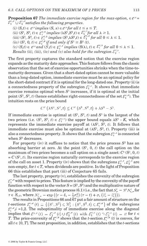
113
Proposition 67 The immediate exercise region for the max-option, ∈εc,x = � satisfies the following properties.
(i) (S,t) ∈ εc,x implies (S, s) ∈εc,x for all t � s � T.(ii) (S1, S2, t) ∈ implies (�S1,S2,t) ∈ for all � � 1.(iii) (S1, S2, t) ∈ implies (S1,�S2,t) ∈ for all 0 � � � 1.(iv) (S1, 0, t) ∈ if and only if S1 � B1 (t).(v) (S,t) ∈ εc,x and ( ,t) ∈ implies (S(�), t) ∈ for all 0 � � � 1.Results (ii), (iii), (iv) and (v) also hold for the subregion .
The first property captures the standard notion that the exercise regionexpands as the maturity date approaches. This feature follows from the classicobservation that the set of exercise opportunities shrinks when the time-to-maturity decreases. Given that a short-dated option cannot be more valuablethan a long-dated option, immediate exercise must be an optimal policy forthe short-dated contract if it is optimal for the long-dated one. Property (ii) isa connectedness property of the subregion . It shows that immediateexercise remains optimal when S1 increases, if it is optimal at the initialpoint (S1, S2, t) (hence establishes right-connectedness of the set ). Theintuition rests on the price bound
If immediate exercise is optimal at (S1, S2, t) and S1 is the largest of thetwo prices (i.e. (S1, S2, t) ∈ ) the upper bound equals �S1 - K, whichrepresents the immediate exercise payoff at (�S1, S2, t). It follows thatimmediate exercise must also be optimal at (�S1, S2, t). Property (iii) isalso a connectedness property. It shows that the subregion is connectedwhen S2 decreases.
For property (iv) it suffices to notice that the price process S2 has anabsorbing barrier at zero. At the point (S1, 0, t) the call option on themaximum of two prices becomes a call option on a single asset: Cx (S1, 0, t)= C (S1, t). Its exercise region naturally corresponds to the exercise regionof the call on asset 1. Property (iv) shows that the subregions , arenon-empty, for t < T, when dividends are positive. In the light of Proposition66 this establishes that part (iii) of Conjecture 65 fails.
The last property, property (v), establishes the convexity of the subregion with respect to prices. This feature is implied by the convexity of the payoff
function with respect to the vector S = (S1, S2) and the multiplicative nature ofthe geometric Brownian motion process (6.1) (i.e., the fact that for� ∈ St,T, where .
The results in Propositions 66 and 67 put a fair amount of structure on thet-sections of the subregions
,i =1,2. The suboptimality of immediate exercise along the diagonalimplies that for t <T. The price-convexity of shows that the t-section (t) is convex, forall t ∈ [0, T]. The next proposition, in addition, establishes that the t-sections
6.3. CALL OPTIONS ON THE MAXIMUM OF 2 PRICES
© 2006 by Taylor & Francis Group, LLC

CHAPTER 6. OPTIONS ON MULTIPLE ASSETS114
diverge from the diagonal as prices increase, before the maturity date. To statethis result define the open cone
for 0 � �2 < �1. The set R(�1, �2) is the cone with vertex at the origin and sidesdetermined by the price ratios �1, �2.
Proposition 68 (Divergence of the t-sections of the exercise region). Foreach t < T there exists a pair (�1, �2) with 0 � �2 < 1 �1 such that εc,x (t) � R(�1,�2) = 0/.
Proposition 66 shows that the diagonal belongs to the continuation region,prior to maturity. Proposition 68 establishes a stronger property: it showsthe existence of an open cone, containing the diagonal, that does notintersect the t-section εc,x (t) (hence belongs to the continuation region). Giventhat the sides of the cone diverge from the diagonal when prices increase, theboundaries of the t-sections will also eventually diverge when prices becomesufficiently large (a formal definition of the boundaries of the sets (t) isprovided in the next section).
Figures 6.2–6.4 illustrate the structure of the exercise region. Figure6.2 shows the behavior of the boundaries near maturity. In this examplethe boundaries of the t-sections converge to piecewise linear functions ast approaches T: for the set (t) the limiting value of its boundary is thediagonal for S2 � K and the strike K for S2 < K. Figures 6.3 and 6.4 showthe t-sections of the exercise region 3 months and 6 months before maturity.The suboptimality of immediate exercise along the diagonal (Proposition66) and the divergence of the t-sections as prices increase (Proposition 68)appear clearly at all maturities. The shrinkage of the exercise region, asmaturity recedes, is also apparent (Proposition 67(i)).
6.3.2 Valuation of Max-Call Options
We now examine the valuation of the contract. The price function Cx (S1, S2,t) exhibits the following features.
Proposition 69 The value of the American max-call option, Cx (S1, S2, t) hasthe following properties:
(i) Cx (S1, S2, t) is continuous on × [0,T].
(ii) Cx (., ., t) is non-decreasing on for all t ∈ [0, T].
(iii) Cx (S1, S2, .) is non-increasing on [0, T] for all (S1, S2) ∈ .
(iv) Cx (., ., t) is convex on , for all t ∈ [0,T].
© 2006 by Taylor & Francis Group, LLC

115
The continuity of the payoff function (S1 V S2 – K)+ with respect to the pricepair (S1, S2) combines with the continuity of the flow generated by stochasticdifferential equations of the form (6.1) (i.e., the continuity of =
with respect to the initial position Si) to produce property(i). The non-decreasing structure of the price function in (ii) is also due to thenon-decreasing behaviors of the payoff and of the flow of the SDE (6.1). Theintuition underlying property (iii) rests on the loss of value associated with areduced set of exercise opportunities (see property (i) of Proposition 67). Theconvexity of the payoff function is the source of (iv).
The continuity of the price function implies that the continuation regionCc,x is an open set while the immediate exercise region εc,x is a closed set.Based on the structure of the exercise set we can define the boundary
Figure 6.2: This figure displays the exercise region of a max-call option one dayprior to maturity. Parameter values are δ1 = δ2 = 6%, σ1 = σ2 = 0.20, ρ = 0, r = 6% andK = 100. Computations use a bivariate version of the binomial model with 400time steps.
6.3. CALL OPTIONS ON THE MAXIMUM OF 2 PRICES
© 2006 by Taylor & Francis Group, LLC

CHAPTER 6. OPTIONS ON MULTIPLE ASSETS116
functions for t ∈ [0, T]. The function represents the boundary ofthe t-section is the boundary of (t). The t-section ofthe exercise region can be rewritten as
The optimal exercise time is the first time at which one of the twoboundaries is crossed
If such a time does not exist set � = T (with the usual convention that thepayoff is null in that event).
Properties of the boundaries can be inferred from the results inPropositions 66, 67 and 68. The function , for instance, can beshown to be non-decreasing and convex in S2, non-increasing in t, bounded
Figure 6.3: This figure displays the exercise region of a max-call option 6 monthsbefore maturity. Parameter values are δ1 = δ2 = 6%, σ1 = σ2 = 0.20, ρ = 0, r = 6% and K= 100. Computations use a bivariate version of the binomial model with 400 timesteps.
© 2006 by Taylor & Francis Group, LLC

117
below by S2 (the diagonal) and such that It has limitingvalue
As for the single asset case has a discontinuity at T if the interestrate exceeds the dividend rate, r > δ1.
The results in chapter 3 show that the max-option price has an earlyexercise premium representation. Based on the characterization of theoptimal stopping time above we introduce the functions
Figure 6.4: This figure displays the exercise region of a max-call option 1 yearbefore maturity. Parameter values are δ1 = δ2 = 6%, σ1 = σ2 = 0.20, ρ = 0, r = 6% and K= 100. Computations use a bivariate version of the binomial model with 400 timesteps.
6.3. CALL OPTIONS ON THE MAXIMUM OF 2 PRICES
© 2006 by Taylor & Francis Group, LLC

CHAPTER 6. OPTIONS ON MULTIPLE ASSETS118
where is defined for a continuous surface
i, j = 1, 2. The function is the value of the European call option onthe maximum of the two prices and is the earlyexercise premium.
Theorem 70 (Early exercise premium representation for max-call options).The value of an American call option on the maximum of two asset priceshas the early exercise premium representation
(6.2)
where is the value of a European call option on the maximum ofthe two assets and is the early exercise premium.The exercise boundaries solve the system of coupled non-linear integralequations
(6.3)
(6.4)
subject to the boundary conditions
(6.5)
(6.6)
At maturity and (S1,t) = K V S1 �B2 (T–) V S1.
Formula (6.2) decomposes the price of the American max-option into a Europeanoption component and an early exercise premium. As usual the EEP componentis the present value of the local gains realized by exercising prior to the maturitydate of the contract. For the max-option the local benefits of exercise can furtherbe decomposed into two parts. Each of these corresponds to the benefits providedby the maximum of the two prices in the event of exercise
Applying the EEP formula at boundary points leads to a system ofequations for the boundary components , . The equations obtainedhave the standard recursive structure. They are also coupled: the integralequation for depends on and conversely. This follows from the
© 2006 by Taylor & Francis Group, LLC

119
fact that the exercise premium, at any given point (S1, S2, t), depends on bothboundary surfaces integrated over future dates and prices.
More explicit formulas can be provided for the European option and theexercise premium components, by using the geometric Brownian motionassumption (see Johnson (1981) and Stulz (1982) for the European optionpart). The resulting integral equations, along with the relevant boundaryconditions, can in principle serve as a basis for the numericalimplementation of the model (see chapter 8 for a description of the integralequation method for the single asset case).
6.3.3 Dual Strike Max-Options
Dual strike max-options generalize max-options. A dual strike max-call paysoff (max (S1 - K1, S2 - K2))+, i.e., it involves a strike price associated with eachone of the underlying asset prices. It collapses to a max-call when the strikeprices are equal.
Let ε c,d be the immediate exercise region of a dual strike max-call option.For each i define the subregion
i = 1, 2. The set is the subset of the exercise region in which the spreadSi - Ki is greatest. The exercise region displays the following properties.
Proposition 71 The immediate exercise region of the dual strike max-callε c,d has the following properties
(i) (S,t) ∈ε c,d implies (S,s) ∈ε c,d for all t � s � T.(ii) (S1, S2, t) implies (�S1,S2, t) for all � � 1.(iii) (S1, S2, t) implies (�S1,S2, t) for all 0 � � � 1.(iv) (S1, 0, t) if and only if S1�B1(t).(v) If S2 = S1 + K2 – K1 and t < T, then (S1,S2,t)∉ε c,d.(vi) (S, t) and ( ,t) implies (S (�) , t) for all 0 � � � 1.Results (ii), (iii), (iv) and (vi) also hold for the subregion
The dual strike call option displays properties that are similar to thosecharacterizing the call option on the maximum of two prices. Prior to maturity,the t-section of the exercise region is the union of two disjoint sets. Thesesubregions lie on each side of the line S2 = S1 + K2 - K1 (the translateddiagonal): immediate exercise along the translated diagonal is a suboptimalpolicy before the maturity date.
An EEP formula for the price of the dual strike max-option can also bewritten as in Theorem 70.
6.3. CALL OPTIONS ON THE MAXIMUM OF 2 PRICES
© 2006 by Taylor & Francis Group, LLC

CHAPTER 6. OPTIONS ON MULTIPLE ASSETS120
6.3.4 Put Options on the Minimum of 2 Prices
The American put option on the minimum of two assets, or min-put option,is also closely related to the call option on the maximum of two assets. Themin-put option payoff is (K – S1∧S2)+ at exercise, S1∧S2 ≡ min(S1, S2)where.Let ε p,m be the immediate exercise region and define the subregions
for i = 1, 2. Also let denote the immediate exercise region of a standardput option on asset i, i = 1, 2. The exercise region satisfies
Proposition 72 The immediate exercise region for the min-put option,ε p,m, has the following properties
(i) (S,t) ∈ε p,m implies (S,s) ∈ε p,m for all t � s � T.(ii) (S1, S2, t) implies (�S1,S2, t) for all 0 � � � 1.(iii) (S1, S2, t) implies (S1, �S2, t) for all � � 1.(iv) (S1, S2, t) implies (S1, t) ∈ (i.e., ⊆ ).(v) (S1, 0, t) .(vi) Suppose (S1, t) ∈ . Then there exists S2*such that (S1, S2, t)
for all S2 � S2*.(vii) If S1=S2 ≠ 0 and t < T, then (S1, S2, t) ∉ ε p,m.(viii) (S1, t) and ( ,t) implies (S (�) , t) for � ∈ [0, 1].Results (ii)–(vi) and (viii) also hold for the subregion .
The properties of the min-put option parallel those of the max-call optionand can be proved using similar arguments. Formulas in the spirit of thosein Theorem 70 can also be provided.
6.3.5 Economic Implications
The analysis performed shows that an American call on the maximum oftwo assets displays unusual properties. The most surprising aspect isperhaps the fact that waiting to exercise is the optimal policy before thematurity date of the contract if the underlying assets have identical prices.Moreover, under these circumstances, waiting is optimal even if theunderlying asset prices or their associated dividend yields are very large.This property of the max-call option stands in sharp contrast with theexercise behavior associated with a standard call option written on a singleunderlying asset.
The diagonal behavior of the optimal exercise policy of the max-calloption has interesting implications for capital budgeting and investmentdecisions involving a choice between multiple exclusive alternatives.Interpreted in that context the result in Proposition 66 shows that economicentities may optimally delay certain investments when the present valuesof the alternatives under consideration are identical. Given that projectsoften involve assets that can be put to multiple exclusive uses this motive
© 2006 by Taylor & Francis Group, LLC

121
for delaying investments is likely to arise in a variety of situations. Thisinsight complements traditional theories of investment behavior under
A complementary property is the divergence of the exercise region: thedistance between the diagonal and the exercise boundaries increases asprices increase (i.e., moving up along the diagonal). Thus, when asset pricesare large, immediate exercise may be suboptimal even if the asset pricesdiffer by significant amounts. Interpreted in the context of investmenttheory this suggests that the adoption of a project among a set of exclusivealternatives may be optimally delayed even if present values are largeand differ significantly.
6.4 American Spread OptionsA call spread option is a contingent claim written on the spread between twoprices, with payoff (S2 – S1,0) – K) + = (S2 – S1 – K)+ upon exercise. When K =0 the spread option becomes an option to exchange asset 1 for asset 2.
Let Cs (S1, S2, t) be the value of the call spread option at the point (S1, S2,t). Relying on the results in chapter 3 we can write
The immediate exercise region is the set
Its t-section is ε c,s (t).
6.4.1 Exercise Region and Valuation
Our next proposition provides key properties of the exercise region.
Proposition 73 The immediate exercise region for a call spread option,ε c,s, has the following properties
(i) (S1, S2, t) ∈ ε c,sand t < T implies S2 > S1 + K.(ii) (S, t) ∈ ε c,s implies (S,s) ∈ε c,s for all t � s � T.(iii) (S1, S2, t) ∈ ε c,s implies (S1,�S2, t)∈ ε c,s for all � � 1.(iv) (S1, S2, t) ∈ ε c,s implies (�S1,S2, t)∈ ε c,s for all 0 � � � 1.(v) (01, S2, t) ∈ ε c,s if and only if S2 � B2 (t).(vi) (S,t) ∈ε c,s and ( ,t) ∈ε c,s implies for all (S (�) , t) ∈ε c,s for all 0 � � � 1.
Most of these properties are intuitive adaptations of those characterizingmax-options (or dual strike options). For property (i) note that the payoffis non-positive if S2 � S1 + K.Proposition 73 implies that the t-section of the exercise region, ε c,s (t), is a
6.4. AMERICAN SPREAD OPTIONS
© 2006 by Taylor & Francis Group, LLC
uncertainty (see Dixit and Pindyck [1994]).
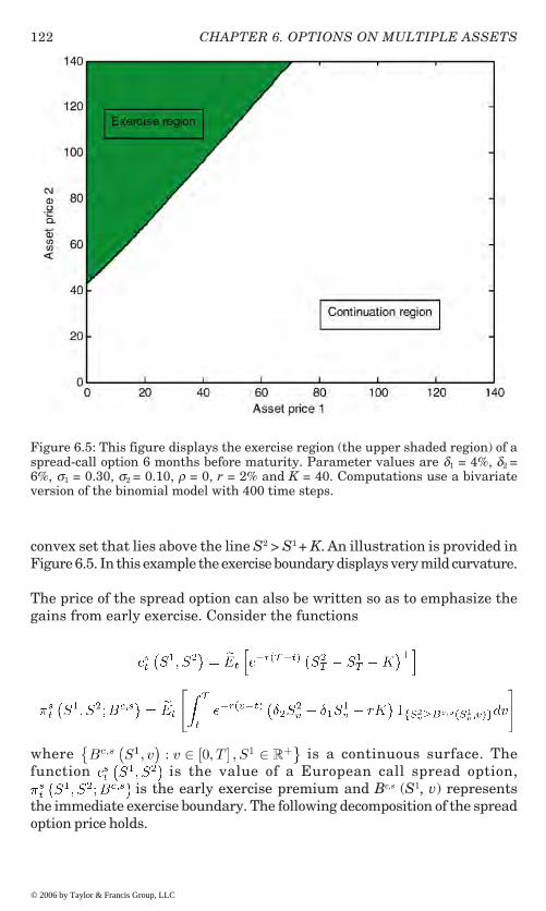
CHAPTER 6. OPTIONS ON MULTIPLE ASSETS122
convex set that lies above the line S2 > S1 + K. An illustration is provided inFigure 6.5. In this example the exercise boundary displays very mild curvature.
The price of the spread option can also be written so as to emphasize thegains from early exercise. Consider the functions
where is a continuous surface. Thefunction is the value of a European call spread option,
is the early exercise premium and Bc,s (S1, v) representsthe immediate exercise boundary. The following decomposition of the spreadoption price holds.
Figure 6.5: This figure displays the exercise region (the upper shaded region) of aspread-call option 6 months before maturity. Parameter values are δ1 = 4%, δ2 =6%, σ1 = 0.30, σ2 = 0.10, ρ = 0, r = 2% and K = 40. Computations use a bivariateversion of the binomial model with 400 time steps.
© 2006 by Taylor & Francis Group, LLC
123
Theorem 74 (Early exercise premium representation for spread options).The value of an American call spread option has the early exercise premiumrepresentation
where (S1, S2) is the value of a European call spread option and (S1, S2;Bc,s)is the early exercise premium. The exercise boundary Bc,s solves therecursive integral equation
subject to the boundary conditions
At maturity .
6.4.2 Options to Exchange One Asset for Another
When the strike is null, K = 0, the call spread option reduces to an option toexchange one asset for another, with exercise payoff (S2 – S1)+ . Using theprice ratio Se � S2/S1 enables us to write (S2 – S1)+ = (Se – 1)+ . The exchangeoption payoff is the same as the payoff of an option written on a single assetwith price Se and unit strike, adjusted by the random quantity S1.
These observations suggest that the change of numeraire approach,reviewed in section 2.7, will be effective in pricing this contract. Giventhat price processes are of the form (6.1), it follows immediately from anadaptation of Theorem 8, with numeraire , that
where
(6.7)
with and where ze is a Brownian motion underthe pricing measure Q* whose Q-density is . TheAmerican exchange option is therefore equivalent to S1 American callswith unit strike, written on a single underlying asset with dividend yieldδ2 and volatility σe, in a financial market with interest rate δ1.
Based on this equivalence one obtains the following result,
Theorem 75 (Early exercise premium representation for exchange options).The value of the American option to exchange asset one for asset two is
6.4. AMERICAN SPREAD OPTIONS
© 2006 by Taylor & Francis Group, LLC

CHAPTER 6. OPTIONS ON MULTIPLE ASSETS124
(6.8)
where is the value of an American optionwith unit strike on an asset with price , dividend yield δ2 and volatility σe,in a market with interest rate δ1. More precisely c( ,t) is the Europeanoption value
(6.9)
and the early exercise premium
(6.10)
where
(6.11)
The optimal exercise boundary Be solves the recursive integral equation subject to the boundary condition .
Formulas (6.8)–(6.11) and the discussion preceding the proposition showthat the American exchange option is symmetric to a standard option pricedin a modified financial market. This symmetry property was first discoveredby Rubinstein [1991] in the context of a binomial tree setting.
The proposition shows that immediate exercise is optimal when theasset price, expressed in the new numeraire, exceeds the boundary,i.e., Equivalently, it is optimal to exercise when .In the plane (S1, S2) the exercise region corresponds to a cone issued fromthe origin whose sides are the ray with slope Be (t) and the vertical axis.This exercise region coincides with the limit of the exercise region for thespread option as the strike converges to zero.
6.4.3 Exchange Options with Proportional Caps
A capped exchange option has a payoff equal to where > 0(equivalently we can write
Note that the payoff function for this contract is non-convex. It alsolacks smoothness in a region where the exercise value is strictly positive(i.e. when It follows that the standard form of the earlyexercise premium representation, as in Theorem 75, does not apply. As forthe case of capped call options, it is nevertheless possible to identify the optimal
© 2006 by Taylor & Francis Group, LLC

125
exercise boundary and to deduce a straightforward valuation formula. Infact the usual change of numeraire reduces this contract to a standard cappedcall in a modified financial market.
Theorem 76 The value of an American capped exchange option withproportional cap (with payoff is given by
(6.12)
where CL( , t;BL) is the value of an American-style capped call option,written on a single asset with price , dividend δ2 and volatility σe (see(6.7)), with strike 1 and cap on the underlying’s price L = + 1, in a marketwith interest rate δ1. Accordingly, immediate exercise is optimal whenS2�BesS1 where the boundary Bec is given by
(6.13)
i.e., the boundary is the minimum of the exercise boundary B for a standarduncapped option on the asset price Se and the cap L. The value of the cappedoption CL( , t;BL) is obtained from Theorems 52 and 53 with the appropriatesubstitutions for the coefficients.
The change of numeraire method proves again very effective in this context.By expressing the payoff in the new unit of account one sees immediatelythat the contract reduces to the familiar form studied in chapter 5. Itfollows that our earlier results apply, with a suitable relabeling of theparameters, and this leads to the formulas in Theorem 76.
6.5 Options on an Average of 2 PricesAn option on a portfolio of assets is an example of a contract whose payoffdepends on an average of prices. Several averaging methods can beemployed. We examine the cases of geometric averaging (section 6.5.1)and arithmetic averaging (section 6.5.2).
6.5.1 Geometric Averaging
For generality we consider a larger class of contracts with payoffs
These are call options on a geometric sum of assets. Special members of thisclass include calls on the power of a product of prices , calls ona product of prices (γ1 = γ2 = 1), calls on a geometric average of assets (γ = 1) andcalls on an equally-weighted geometric average of assets (γ1 =γ2 = 1/2).
A simple argument establishes that these options are effectively written
6.5. OPTIONS ON AN AVERAGE OF 2 PRICES
© 2006 by Taylor & Francis Group, LLC

CHAPTER 6. OPTIONS ON MULTIPLE ASSETS126
on a single underlying asset. Defining and applying Ito’slemma gives
(6.14)where
One concludes that Y follows a geometric Brownian motion process withimplicit dividend yield δY and volatility coefficient σY. As (6.14) does notdepend on the original prices S1, S2, we conclude that the geometric sumoption is identical to an option written on Y alone. To proceed, let us assumethat δY � 0 (if the implicit dividend δY is negative there are no incentivesto exercise early). Also let be the optimal exercise boundary ofan American call on Y and let Ct (Y) be its value.
Theorem 77 The optimal exercise boundary for an American geometricsum option is
(6.15)
where is the exercise boundary for the single asset call written on the processY given in (6.14). The option value is where C(Y, t) is the value of theAmerican call on Y.
As announced by the discussion preceding the proposition the option on ageometric sum is identical to an option written on asset Y alone. The decisionto exercise can be based directly on Y: immediate exercise is optimal at thefirst time at which Y equals the boundary B. Alternatively, the decision canbe based on the two underlying assets. If asset 2 is taken as the referenceasset then immediate exercise is optimal at the first time at which S2 reachesthe boundary Bgs (S1, t) described in the proposition. As could have beenexpected, this boundary is a non-linear transform of B, where the degree ofnon-linearity depends on the parameter γ2. The relation also depends on theprice of asset 1 and the associated power γ1.
6.5.2 Arithmetic Averaging
Consider an American option written on a weighted average of asset priceswith constant weights. The underlying asset in this contract can be viewed
© 2006 by Taylor & Francis Group, LLC
127
as a portfolio of two assets. The analysis of this type of contract is useful as italso helps to shed light on the structure of the exercise region for a morecomplicated contract, the min-option (see section 6.6)). The payoff on a calloption upon exercise is (wS1 + (1 - w) S2 - K) , where w ∈ (0, 1). The choice w= 1/2 corresponds to a call on the arithmetic average of two prices. The nextproposition describes the optimal exercise region. We recall that Bi denotesthe exercise boundary of a call option on asset i, i = 1, 2.
Proposition 78 Let ε c,w be the optimal exercise region for a call option onthe weighted average of 2 prices where w ∈ (0, 1) is constant. Then
(i) (0, S2, t) ∈ε c,w if and only if .
(ii) (S1, 0, t) ∈ε c,w if and only if .
(iii) (S1, S2, t) ∈ε c,w implies (�1 S1, �2,S2, t) ∈ε c,w with �1 � 1, �2 � 1.(iv) (S, t) ∈ε c,wand ( ,t) ∈ε c,w implies (S (�), t) ∈ε c,w for all � ∈ [0, 1].(v) (S1, S2, t) ∈ε c,w implies (S1, S2, s) ∈ε c,w for T � s � t.
Most of these properties are intuitive. Property (iii) establishes thatimmediate exercise remains optimal when both prices increase. Thisfeature follows from the upper bound on the payoff function
that holds for �1, �2 � 1. The payoff bound implies the price bound
As immediate exercise is optimal at (S1, S2, t) the price bound becomes w�1S1
+ , the exercise value at the point (�1S1, �2S2, t). Immediateexercise must therefore be an optimal policy at the point (�1S1, �2S2, t).
Figure 6.6 illustrates the exercise region for a weighted average option.A valuation formula is given next.
Theorem 79 (Early exercise premium representation for weighted averageoptions). The value of the American call option on a weighted (arithmetic)average of two assets is
where cw (S1, S2, t) is the value of the European option on the weighted average
6.5. OPTIONS ON AN AVERAGE OF 2 PRICES
© 2006 by Taylor & Francis Group, LLC

CHAPTER 6. OPTIONS ON MULTIPLE ASSETS128
Figure 6.6: This figure displays the exercise region (the shaded region) of an equally-weighted average call option 6 months before maturity. Parameter values are δ1 =δ2 = 6%, σ1 = σ2 = 0.20, ρ = 0, r = 6% and K = 100. Computations use a bivariateversion of the binomial model with 400 time steps.
where
© 2006 by Taylor & Francis Group, LLC

129
and
with .The optimal exercise boundary solves
subject to the boundary condition .
6.6 Call Options on the Minimum of 2 PricesAn American call option on the minimum of 2 asset prices has an exercisepayoff given by Let Cm (S1, S2, t) be its price. Theimmediate exercise region is the set
Its complement is the continuation region C c,m .
6.6.1 Exercise Region of a Min-Call Option
As for the max-option, it is of interest to examine the behavior when oneasset, or the other one, is more expensive. This partition corresponds tothe subregions i = 1, 2.
Taking the intersection with the exercise region leads to the subsets for i = 1, 2. Here is the subset of the exercise region
in which asset i is more expensive. With these definitions, it is clear thatthe intersection , if non-empty, belongs to the diagonal. Given
that some of the results presented involve options on individual assets we
also need the exercise region εi for a call option on asset i along with the
boundary Bi, i = 1, 2. Similarly, we recall that ε c,w represents the exerciseregion of a call option on a weighted average of two assets. Thecorresponding boundary is Bc,w.
The next proposition identifies key properties of ε c,m , and .
Proposition 80 The immediate exercise region of an American min-calloption, ε c,m has the following properties
(i) (S, t) ∈ ε c,m implies (S, s) ∈ ε c,mfor all t � s � T.
6.6. CALL OPTIONS ON THE MINIMUM OF 2 PRICES
© 2006 by Taylor & Francis Group, LLC
CHAPTER 6. OPTIONS ON MULTIPLE ASSETS130
(ii) (S,t) ∈ε 2 and (S1, S2, t) ∈G1 implies (S1, S2, t) ∈ .(iii) (S1, S2, t) ∈ implies (�S1, �S2) ∈ for all � � 1.(iv) (S1, S2, t) ∈ implies (S1, �S2, t) ∈ for all 1 � � � S1/S2.(v) (S1, S2, t) ∈ implies (�S1, S2, t) ∈ for all S2/S1 � � � 1.(vi) (S1, S2, t) ∈ ε c,w for w ∈ (0,1) and S1 = S2, implies (S1, S2, t) ∈ ε c,m
(vii) (0, S2, t) ∉ ; (S1, 0, t) ∉ ε c,m.Results (ii)–(v) also hold for the subregion .
Property (i) is standard. Result (ii) states that immediate exercise isoptimal for the min-option if it is optimal for a standard option on asset2 and asset 2 is cheapest. This is true because the min-option payoff canattain, but never exceed, the payoff of a call option on asset i, i = 1 or 2.The min-option price is then bounded above by the prices of the two calloptions written on the individual asset prices. If immediate exercise isoptimal for one of these two calls and the min-option attains the samepayoff, it will also be optimal to exercise the min-option. Property (iii)shows that the subregion is ray-connected: increasing both pricesby a common factor preserves the optimality of exercise. The subregion
is also up-connected (see (iv)) and left-connected (see (v)). Of course,by the definition of , these connectedness properties only extend upto the diagonal.
Property (vi) highlights an interesting relation between the weightedaverage option and the min-option. It is easy to verify that the payoff ofthe min-option is bounded above by the payoff of the average option
with equality along the diagonal (where S1=S2). As a result, if immediateexercise is optimal along the diagonal for the holder of the average option,it will also be optimal for the min-option.
The last statement, (vii), expresses the simple intuition that immediateexercise cannot be optimal along the two axes because the payoff is null.
Proposition 80 suggests an exercise region whose boundary can bedescribed by two surfaces corresponding,respectively, to the subregions and . These surfaces meet andmerge along the diagonal. Their common lower extremity, along thediagonal, is a curve parametrized by time. Thus, (S1, S2, t) ∈ ifand only if S2 = min (S1, S2) � (S1, t). Similarly, (S1, S2, t) ∈ if andonly if S1 = min (S1, S2) � (S2, t). Finally, (S, S, t) ∈ ε c,m if and only ifS � . Figure 6.7 illustrates this structure.
Associated with the properties of the exercise region are the followingproperties of the boundaries.
Proposition 81 The boundary has the following propertiesover its domain,
© 2006 by Taylor & Francis Group, LLC

131
(i) (S,t) is a non-increasing function of time.(ii) (S,t) is non-decreasing in S2 and bounded above by B1 (t).(iii) If for i = 1, 2 and then (x, t) = x for
all .(iv) (v)
= K.(vi) Let
where x* (t) uniquely solves Bc,w (x, t) = x.Analogous properties hold for the boundary of the region .
The first 2 properties are direct consequences of (i), (ii) and (v) ofProposition 80. Property (iii) states that the diagonal boundary componentis connected in the price direction (i.e., if two pairs of asset prices lie onthe diagonal and belong to the exercise boundary then every intermediatediagonal pair also belongs to the exercise boundary). This parallels the
Figure 6.7: This figure displays the exercise region of a min-call option 6 monthsbefore maturity. Parameter values are δ1 = δ2 = 6%, σ1 = σ2 = 0.50, ρ = 0, r = 6% andK = 60. Computations use a bivariate version of the binomial model with 1500 timesteps.
6.6. CALL OPTIONS ON THE MINIMUM OF 2 PRICES
© 2006 by Taylor & Francis Group, LLC

CHAPTER 6. OPTIONS ON MULTIPLE ASSETS132
behavior of the exercise region, along the cap, for a capped call option (seechapter 5).
The limit in (iv) follows from the fact that the payoff of the min-optionconverges to the payoff of an option on asset 1 alone as S2 becomes large. Thesame reasoning applies for the first limit in (v). As maturity approaches, andif S1 is strictly less than S2 then the min-option converges to an option onasset 1. Accordingly, the min-option boundary converges to the limiting valueof the boundary for that single asset option. For the second limit in (v), alongthe diagonal, convergence is toward the strike, even if the dividend yields onboth assets are low. This may appear puzzling at first sight. The explanationis similar to the one for the suboptimality of exercise along the diagonal formax-options. To simplify matters consider the case where asset prices areindependent, have identical volatility coefficients and dividend yields equalto the interest rate. The probability of an improvement in the minimum oftwo prices, along the diagonal, is only about 1/4 (the likelihood of a decreaseis about 3/4). Thus, as maturity approaches, it will pay to cash in any positivepayoff no matter how small. In the limit, the policy of waiting to exercise isdominated as long as the option is in the money and asset prices are equal.
The results above show that the stopping time problem reduces to theidentification of the two surfaces and and of thecurve along the diagonal (compare this to the (te, t*, tf)-policies thatare optimal for capped options with growing caps). Integral equations forthese curves are provided below.
6.6.2 The EEP Representation
As usual the derivation of integral equations for the boundary componentsrelies on the EEP representation of the option price. To establish thisformula in the case of a min-call one has to deal with a non-smooth payofffunction with discontinuous derivatives across the diagonal. The existenceof these discontinuities implies that the standard version of Ito’s lemmacannot be used to describe the behavior of the minimum price processS1^S2. Instead we must rely on an extension of the Ito rule, the Tanaka-
6.8]), that applies to convex functions.Define to represent the minimum price. For any fixed t,
and be the discounted payoff of themin-option. An application of the Tanaka-Meyer formula establisheswhere, for a process x, L (u, 0; x) is the local time of x at the point zero and
© 2006 by Taylor & Francis Group, LLC
Meyer formula (see Karatzas and Shreve [1988, Chapter 3, Proposition

133
is the local variance of the difference in returns(or, equivalently, in log-prices).1 This gives a decomposition of the form(3.8) for the payoff process Y. From Theorem 21 we now obtain the followingEEP representation of the option price (note that dL (u, 0; X - K) = 0 in theexercise region of the min-option),
Theorem 82 The price of the min-call option has the early exercise premiumrepresentation
,
where is the price of the European min-call option and the function
is the early exercise premium
with components
and where As usual the EEP formula decomposes the option value into a European
component, capturing the value of waiting to maturity, and an earlyexercise premium, representing the benefits associated with early exercise.
1When x is a Brownian motion the process L (u, 0; x) is the Brownian local time defined as
6.6. CALL OPTIONS ON THE MINIMUM OF 2 PRICES
© 2006 by Taylor & Francis Group, LLC

CHAPTER 6. OPTIONS ON MULTIPLE ASSETS134
Unlike the standard case, the exercise premium is the sum of two parts. Thefirst part is the present value of the net flow gains (i.e., dividends net ofinterest costs) from early exercise, . The dividend benefits, for thiscontract, are those associated with asset 1 (resp. asset 2) when S1 (resp. S2) isthe minimum of the two prices. The second part, , is due to the lack ofsmoothness in the payoff function, in the exercise region, along the diagonal.Every time the minimum of the two prices crosses the diagonal the derivatives,with respect to prices, of the payoff function jump. The local time process L(t, 0; In (S1) - In (S2)) compensates for these jumps: the increment dL is non-negative at all times, and strictly positive along the diagonal. Thus, isnon-negative. Intuitively, exercising the option along the diagonal saves valuegiven the higher likelihood of a decrease in the minimum price, and theoption payoff, over the next instant of time.
The formula for provides additional perspective about the behavior ofthe contract along the diagonal. Note, for example, that the variance ofthe return differential is positive (i.e ) except when returns areperfectly correlated and carry the same risk (i.e., σ1 = σ2 and ρ= 1). Whenthese conditions prevail underlying prices satisfy the deterministic relation
, with . The min-option is thenequivalent to a call option written on a single asset, with a quantityadjustment that depends on time: the option’s payoff takes the form
. The smoothness of this contractualstructure, with respect to the underlying Brownian motion, implies thatthe local time component disappears from the EEP representation.
Note also that the min-option is identical to a capped call option withtime-dependent cap when either σ1 = 0 or σ2 = 0 (see chapter 5 and section6.4.3 above). Our previous analysis of this contract led to a pricing formulaemphasizing the gains from exercising before hitting the cap (see Theorem53). The price decomposition in Theorem 82 provides an additionalrepresentation of capped option prices, highlighting the benefits ofexercising before the maturity date of the contract. This expression, in thespirit of traditional EEP formulas, prices the early exercise premiumrelative to a European capped call option.
When , the premium component is positive and the exerciseboundary consists of the three parts , and identifiedabove. If the underlying assets do not pay dividends (δ1 = δ2 = 0). there areno incentives to exercise off the diagonal. In this situation the premia vanish and the boundary curves , collapse to thediagonal: the exercise region is the subset of the diagonal above .
Before moving on to the next section let us also point out that some ofthe EEP components can be expressed in more explicit form. A formulafor the European min-option price can be found in Johnson [1987]. Moreexplicit formulas can also be derived for the components of theearly exercise premium.
© 2006 by Taylor & Francis Group, LLC

���
������������� ��������������������������������
����������������� ��������������������������������� ����������������������������� ���������� �������������������������� ������� �� ����������������� ������ �� ������������������ ���
������� ������� �������� �� �� � � � ���������������������������������������������������
�������������������������������
����� ��� ���� �� ��� ���� ���� � ������ �������� � ������������������ ��� ������������������� ���� ������������� �
��! ��� ����������"������������������������������ �������������#��� �� ���� �� ���� ���� ���� ���� ��������� ���������������� �� � ��� � ������ �� ������� ��� ����������������� � ���������������� �� ���
�� ���������� ������������������ ���������������������������������� ��������������� ��������� ����$%������������������������
��� ��������� ���� � ������������ ���������������� � � ���������� ���� ������������������ ������� ��������� �� ������������������������������ ������������ ������ ����������������������������������������������������������� ����������������������������� ������� ������������� ������� ������������������� ������ �����������"����� �� ������������������������� ������������� ��
�������������� ��������������������������
#�������������������� ��������������������� ����������������� �������������� ���� ��������������������� ���������������������&������ ���������������� ������������������'�������������"��������������(
')�*)(
������ � ��� �������+� ������ �� �� �� ������� ��� ���� ������ ���������� � ����� �������������� ���������� �����������
���������������� ������������������������
© 2006 by Taylor & Francis Group, LLC

������ �������������������������������
�����,��������������������� ������������������������ ����������')�*)(���������������������������"��������� ����&������������������������� ������ ������������ ������ ����� ���� ���- ����������� �������������������������� ��� ������� �������������������. ��������� �������� ���������������������� �����������������
�������')�*)(�������������������������/��� ������������� ������������������ ����� �� ����� ���,��0 ��� ����������� ������� ���������� ������� �� ��1�� ������������ ���������������������������������0� ���������%�������
2
���������������������� ���� ������������ ������������� ���������������� ���!��������������������������� ����� �&������ �������� ����������� ���� ���������������� �� ���� � ���� �
%*�� 3��� � ��� � ������� � �� ������ ������ ������ ���� ���� ������� �� ��������� ��� ���� ���������
� ��� ��������� � � ���� ������� �� ��������� ��� ���� ���+� ������ �� �
2
�����������
2
������ ������� �������������"�������������4,��*5� ������������� �������������� �#������� �� �������������"�#�'��"���6����"�(��� ��������������� �������������������� ��� ����� ����&������������������ �������������
2�
������������������ ������"������������ ������� ����� �� ���������� ��� ��������������������������� ��� ������������� ���$�� ��������������� ���������� ���������� ������������ ������������7����������� � ���� ���� ��������� ���� ��� ����������������� �����
������������� ��������������� �����
������������������������������������������������������������%�������������� ���������������������������������������������������������������������&�������������������� �������������������������
�����������������������. ����������������� ����������� ������� ������������������� ��8��������������� ���������������� ������
© 2006 by Taylor & Francis Group, LLC

���
���������������������� ������������������������������������������������������������� ���������� ����������� ��������������������������������������������������������������������������������
������ ���
!
�����������������������������������������������������������������������"�����������#$�%������������������������������� ���������� ��������������������������������������������� ��������������������������� ��������������������������������������������
��������������� ����������������������������������������������������� �!������"�������� ##������$����������������������"������������������������������������������$�$������������������"�������"���������������������������������� ##�#������������#��
�&��'�
����������(�������������������������������#�%����� �����������$���������������
�&��#�
#������������� ����������������������&$'(��$�!���� $
������������������� ����������������������� ��������������������� ��������������� ������������ �������������)�����
���� ������������ ������������������������
© 2006 by Taylor & Francis Group, LLC

��� ������ ����������������������������
*���������������������������������)������������������������&��'������&��#�������������������� ��+�����������������������%����� ������� ��*����������������
!
����&��'�������������,���-��������������&��#���������������������������� �
!
.����,�������
!
�����������������������������������/�%��������/�%������������%�������*�����������������������������������&��'������&��#�����������,�0����
������������������������������������������� ������������������������
������������������������������ ���
1�����������&��'������&��#���������������������������%��������������������������������������������������2
© 2006 by Taylor & Francis Group, LLC
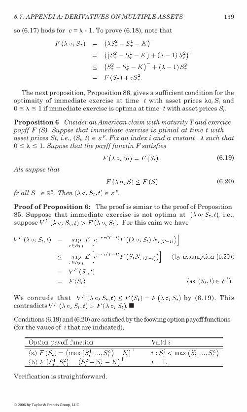
���
������ ���������������"�����������#&��%������������������������������������������� ��� ��������� � ������� �� ����� ������� ����� ��������o����� ��(���������������������� ���������������������������������������������
���������������������������������������������� �!������"������� ##��� ���$�������� ����� ���������"������ ����������� ���� ���������������������$�$������������������"�������"���������������������������(���������������������������� ##�#������������#��
�&��3�
���������������
�&�0(�
#������������� ��!���� ������$
������������������� ������������������������������������"����������#$�� �������� ���� ��������� � ������� ��� ���� ������ �� �� ������������� ���*������������������
����&��'�������������,���-��������������&��#�����������
)�� �������� ���� � ��� �&��3��� ��������������� ���
1�����������&��3������&�0(���������������������������%����������������������������������������������������������
4������������������%���������
���� ������������ ������������������������
© 2006 by Taylor & Francis Group, LLC

��� ������ ����������������������������
*��������������������������������������������������
!
"�����������#'�%����������������������������������������� ���������������������������������������������������������'�������������� ��������������������������������������������
���������������� ������������������������������������������������ �!������"�������� ##������$����������������������"������������������������������������������$�$���������������������������������#������������������ ##�#������������#��
�&�0��
����������(�������������������������������#�����%����� ���������������������������
�&�00�
#������������� $�!����#������������������)����������������
������������������� �������������������������������� ������*��� 5� ������������� ������ ����� ���� ������%� �����%� ������������
���������������������������������������������
1�����������&�0�������&�00�������������������������������������������
�����������������������������������������������������������������������������*(��)����������
© 2006 by Taylor & Francis Group, LLC

���
���������������������������������������������������������������������������
����&�0��������������,����-����+������������&�00���������������������
����&�0��������������,����-���+������������&�00��
�����������������������������������������������������������������������(��)���������
����&�0�������������,���-���+������������&�00����������
"�����������##�������������������������� ���������������������������� �������%�����������
���� ������������ ������������������������
© 2006 by Taylor & Francis Group, LLC

��� ������ ����������������������������
.��������������������"������������#$����#&��������������� ����������������������������������������������������-��������������
��������������,���� ���������������������������������������������������� �!������"�������� ##������$����������������������"������������������������������������������$�$���������������$��"�������"������������������������"������#��������
� ����������������#�� ������� ##�#������������#��
�&�06�
��������,�(�������������������������������#�����%����� ����������-����������������
�&�07�
#������������� �����������������������&$./��$�!���� �������#�������
����8 �
������������������� ��������������������������������������������������
��������o����������������� �����������������������������8 �)�����
���������������)�"� ������������������������������������ �!�����"�������� ##������$�������������������������� ����)�"�#�����$!����������������������� ����)�"����������������$
������������������ �9���%���������� �������������������������������������
�
© 2006 by Taylor & Francis Group, LLC

143
Proposition 90 (Left-segment-connectedness): Consider an American claimwith maturity T and exercise payoff F (S). Suppose that immediate exerciseis optimal at time t with asset prices St, i.e., (St, t) ∈ ε F . Fix an index j andsuppose that there exists a function (.):Rn
+ → R such that, for h (St) ≤ � ≤ 1,the payoff function F satisfies
(6.25)
Also suppose that
(6.26)
for all S ∈ Rn+ . Then (��j st,t) ∈ ε F for h (St) � � � 1.
Proof of Proposition 90: Suppose that immediate exercise is not optimalat (� oj St, t), i.e., VF (� oj St, t) > F (� oj St). We have
This contradicts our assumption . �
Conditions (6.23) and (6.24) are satisfied by the min-option payoff F (St) =
Hence by (6.25). This contradicts theassumption that .�
For min-options the proposition holds for any index j � i where i : Sit = min
(S1t, …, Sn
t). The function h (.) is h (St) Sit/Sj
t.
6.8 Appendix B: ProofsProof of Proposition 66: The argument following the proposition showsthat the American-style max-option price is bounded below by the value ofa package consisting of a forward contract and a European exchange option.That is,
6.8. APPENDIX B: PROOFS
(by (6.26))
(as (St, t) ∈ ε F).
© 2006 by Taylor & Francis Group, LLC
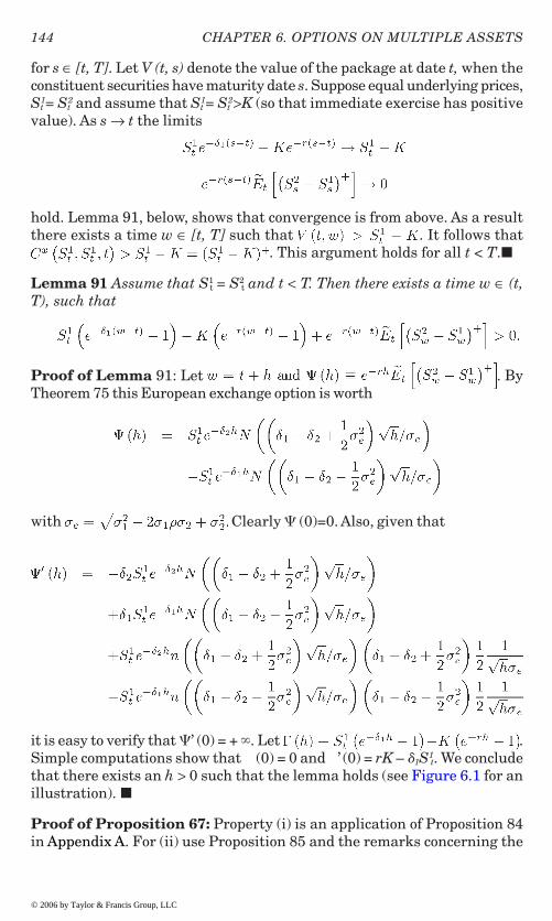
144 CHAPTER 6. OPTIONS ON MULTIPLE ASSETS
for s ∈ [t, T]. Let V (t, s) denote the value of the package at date t, when theconstituent securities have maturity date s. Suppose equal underlying prices,St
1= St2 and assume that St
1= St2>K (so that immediate exercise has positive
value). As s → t the limits
hold. Lemma 91, below, shows that convergence is from above. As a resultthere exists a time w ∈ [t, T] such that . It follows that
. This argument holds for all t < T.�
Lemma 91 Assume that S1t = S2
t and t < T. Then there exists a time w ∈ (t,T), such that
Proof of Lemma 91: Let . ByTheorem 75 this European exchange option is worth
with Clearly � (0)=0. Also, given that
it is easy to verify that �’ (0) = + . Let .Simple computations show that (0) = 0 and ’ (0) = rK – �1S1
t. We concludethat there exists an h > 0 such that the lemma holds (see Figure 6.1 for anillustration). �
Proof of Proposition 67: Property (i) is an application of Proposition 84in Appendix A. For (ii) use Proposition 85 and the remarks concerning the
© 2006 by Taylor & Francis Group, LLC

145
payoff function (a) following that proposition. For (iii) use Proposition 86and the subsequent remarks for payoff function (a). For (iv) note thatS2
t = 0 implies S2s = 0 for all s � t. In this event the max-option reduces to a
single asset option written on the price S1, whose exercise boundary is B1.To prove (v) note that the convexity of the payoff function and Proposition88 enable us to write
By assumption . It then follows that Cx(S(�), t)�
. Suppose now that immediateexercise is suboptimal at (S (�), t), that is Si (�) – K. This contradicts the previous inequality. We conclude that (S(�) , t) ∈ . �
Proof of Proposition 68: Let εc,x be the exercise region at date t,parametrized by the strike K and let Cx (S1, S2, t; K) be the correspondingmax-option price. The proof uses the next three lemmas documentingproperties of the exercise region.
Lemma 92 K1 > K2 = 0 implies . In particular, K1 >K2 = 0 implies .
Proof of Lemma 92: The proof proceeds by contradiction. Let K1 > K2 � 0and suppose that . We show thatthis combination of assumptions is not possible.
The following string of relations holds
The inequality on the first line expresses the suboptimality of exercise at (S,t) for the max-call with strike K2 (i.e. (S,t) ∉ ε c,x (t, K2)). The second line isthe pricing formula for the American-style max-option. The third line is astraightforward decomposition of the option payoff (�2 > t is the optimal exercisepolicy for the option with strike K2). The inequality on the fourth line resultsfor the bound (a + b)+ � a+ + b+. The next inequality follows from r � 0.
6.8. APPENDIX B: PROOFS
© 2006 by Taylor & Francis Group, LLC

146 CHAPTER 6. OPTIONS ON MULTIPLE ASSETS
Finally, the last line uses the optimality of exercise at (S, t) for the max-callwith strike K1 (i.e. . The resulting contradiction showsthat immediate exercise must be optimal at (S, t) for the strike K2 if it isoptimal for the strike K1.
The case K2 = 0 is an application of the general result. �
Lemma 93 (Ray connectedness) ε c,x (t,0), for all � > 0.
Proof of Lemma 93: The proof is by contradiction. Let and assume that there exists � > 0 such that . Letting
denote the optimal policy at (�S1, �S2, t) (for an option with nullstrike) we can write
(the last inequality follows from the feasibility of τ� at (S1, S2, t)). We concludethat , in contradiction with the initial assumptionthat
Lemma 94 (Diagonal behavior) .
Proof of Lemma 94: The lemma is a particular case of Proposition 66 withK = 0. �
Let us now return to the proof of Proposition 68. By Lemma 94 (S, S, t) ∉ε c,x (t, 0). Given that the continuation region is an open set there exists anopen neighborhood N of the point (S, S) such that S1, S2, t) ∉ ε c,x (t, 0). for all(S1, S2) ∈ N. Lemma 93 then shows the existence of an open cone R (�1, �2),containing the diagonal, such that . Lemma 92enables us to conclude that
Proof of Proposition 69: Property (i) can be proved by using arguments inBroadie and Detemple [1997] and Jaillet, Lamberton and Lapeyre [1990].The property rests, in particular, on the continuity of the discounted payofffunction and the continuity of the flow of the stochastic differential equationfor Si, i = 1, 2. Property (ii) can be proved by using the Comparison Theorem
the payoff function is non-decreasing in prices. Property (iii) is thecounterpart of property (i) in Proposition 67. Convexity, in property (iv),results from the convexity of the payoff function (see Proposition 88). �
© 2006 by Taylor & Francis Group, LLC
for solutions of SDEs (see Karatzas and Shreve [1988]) and the fact that

147
Proof of Theorem 70: The EEP formula follows from Theorem 21 extendedto the case of multiple underlying assets. The particular structure of theexercise premium follows from the geometry of the exercise region delimitedby the two boundary surfaces Bc,
1x and Bc,
2x. The recursive integral equations
for the boundaries are obtained by evaluating the contract along each ofthe boundaries. �
Proof of Proposition 71: Property (i) follows from Proposition 84 in AppendixA. For (ii) and (iii) apply Propositions 85 and 86. Property (iv) holds becausethe dual strike max-option collapses to an option on asset one alone when S2
= 0. The case S2 = S1 + K2 - K1, in property (v), corresponds to the case of thediagonal for max-options. When S2 - K2 = S1 - K1 a movement away from theline S2 = S1 + K2 - K1 provides good odds of improving the payoff. This can beformally demonstrated using the arguments in the proof of Proposition 66.The convexity property (vi) follows from Proposition 88. �
Proof of Proposition 72: Properties (i), (ii) and (iii) are straightforward.Property (iv) follows because the payoff of a min-put option is bounded belowby the payoff of a plain vanilla put on asset 1. Under the assumption of property(v) the min-put option has maximal payoff K, which implies optimality ofimmediate exercise. For (vi), suppose that there is no threshold S2* > S1 suchthat for all S2 � S2*. It must then be that
. But the limit on the left hand side is thevalue of a put on asset 1. This contradicts the assumption . For(vii) note that a deviation from the diagonal has high probability of increasingthe payoff. Dominance of waiting can be formally proved as in the proof ofProposition 66. Convexity in (viii) follows from Proposition 88. �
Proof of Proposition 73: For assertion (i) note that immediate exercisewhen would generate a non-positive payoff. Property (ii) is aspecial case of Proposition 84 in Appendix A. Assertion (iii) follows fromProposition 85 and the subsequent remarks for payoff function (b). For(iv) use Proposition 86 and the remarks that follow for payoff function (b).To prove (v) note that . In this situationthe spread option reduces to an option on on asset S2, with exerciseboundary B2. The proof of (vi) follows from Proposition 88. �
Proof of Theorem 74: The EEP formula for the spread option is anapplication of Theorem 21 generalized to multiple assets. The particularstructure of the exercise premium follows from the geometry of the exerciseregion detailed in Proposition 73. Standard arguments lead to the recursiveintegral equation. �
Proof of Theorem 75: The proof applies the change of numeraire outlinedin section 2.7. To establish the proposition we need to verify the dynamicsof the process Se under the new pricing measure.
6.8. APPENDIX B: PROOFS
© 2006 by Taylor & Francis Group, LLC

148 CHAPTER 6. OPTIONS ON MULTIPLE ASSETS
Let Se = S2/S1. An application of Ito’s lemma gives
where . Under the pricing measure Q* suchthat
the translated process is a Brownian motion. Using for some orthogonal Q-Brownian motion yields
with the definitions
Theorem 8 can now be applied, with numeraire to establishthe symmetry result stated. The EEP representation and the integralequation for the boundary follow immediately. �
Proof of Theorem 76: The option value can be transformed in thefollowing manner
where the last equality uses the passage to the new measure in whichasset 1 is the numeraire (see proof of Theorem 75). The results in theproposition follow from this transformation. �
Proof of Theorem 77: The option with geometric sum payoff is identicalto an option on a single asset with price dynamics
where
© 2006 by Taylor & Francis Group, LLC

149
and
Let B denote the exercise boundary of the option written on Y. The boundaryof the average option is obtained by solving the equation
B (t). The value of the option is the value of the option
written on asset Y. �
Proof of Proposition 78: The claims (i) and (ii) are straightforward. Theproof of (iii) is by contradiction. Suppose that immediate exercise is optimalat (S1, S2, t) but not at (�1S1, �2S2, t) where �1, �2 � 1. Let �� > t be the optimalpolicy at (�1S1, �2S2, t). Standard arguments can be applied to show thatThe resulting contradiction proves (iii).
The convexity result in (iv) is a special case of Proposition 88 in AppendixA. The proof of (v) is standard (see Proposition 84). �
Proof of Theorem 79: The EEP representation gives
where
The event of exercise can be written as and is equivalentto with
6.8. APPENDIX B: PROOFS
© 2006 by Taylor & Francis Group, LLC

150 CHAPTER 6. OPTIONS ON MULTIPLE ASSETS
and . Using we obtain
with
With h = v - t, the conditional expectation inside the early exercise premium w is
where
To simplify the notation let z � z1. Simple transformations give
and it is straightforward to verify that the double integral in �2(v) equals
Substituting the function
© 2006 by Taylor & Francis Group, LLC

151
in the formulas above gives the result stated. �
Proof of Proposition 80: Property (i) follows from Proposition 84. For (ii)it suffices to note that the min-option payoff is bounded above by the payoff ofthe option on asset i, i = 1, 2. Properties (iii)–(v) are special cases of Propositions87, 89 and 90.
For (vi) note that the min-option payoff function satisfies the bound
for w ∈ (0, 1). The price upper bound follows.Suppose now that immediate exercise is optimal at a point along thediagonal, for the weighted average option: and S1 = S2. At this point the previous inequality becomes
. Given thatimmediate exercise is feasible for the min-option we also have the lowerbound , i = 1, 2. The resultfollows.
For (vii) it suffices to note that the payoff is null along the axes. �
Proof of Proposition 81: Statements (i) and (ii) are direct consequencesof (i), (ii) and (v) in Proposition 80.
To prove (iii) let . Consider a point. The ray connectedness property of the exercise region (prop-
erty (iii) in Proposition 80) implies that immediate exercise is optimal alongthe diagonal above hence at the point (S, S). Thus, .Suppose that the inequality is strict: . Given that the exerciseregion is closed, a property that follows from the continuity of the price function,we have . Ray-connectedness then shows that
for any � ≥ 1. Selecting establishesthat . But, by assumption,
. Multiplying each side of this inequality by produces, a contradiction. It follows that
Let us now establish the limit in (iv). By (ii) we know that is non-decreasing in S2 and for all S2 > S1. Supposethat and consider a price S1 such that
For all S2 ≥ S1 we have S1–K=Cm (S1,S2,t). Taking the limit as S2 →∞, andusing the continuity in (S1, S2) of the price function gives
6.8. APPENDIX B: PROOFS
© 2006 by Taylor & Francis Group, LLC

152 CHAPTER 6. OPTIONS ON MULTIPLE ASSETS
Given that (i.e., when S2 goes to infinity any exercisepolicy for the option on asset 1 becomes feasible for the min-option) we conclude
. This contradicts our assumption S1 < B1 (t) (i.e.,immediate exercise is suboptimal for C (S1, t) at S1, so that
. This proves the limit stated.
For the first limit in (v), note that (ii) also implies . To establish the reverse inequality we need to
show that implies . The case K ≥ rK/�1 istrivial because implies S1 � K. We consider the caserK/�1 > K next.
The proof is by contradiction. Suppose that while S2 >S1 and S1 < rK/d1. We show the existence of an arbitrage opportunity.
The optimality of immediate exercise implies Cm (S1, S2)=S1– K≥0. onsiderthe portfolio comprised of a long position in one call option, a short position in oneshare of the asset 1 and an investment of K dollars at the riskless rate. Theinitial cost of this portfolio is null. Suppose that we adopt the portfolio liquidationpolicy
Clearly � > t because S2 > S1t and S1 < rK/�1. The portfolio payoffs generated
by this policy are given by
As the cash flow at τ is strictly positive (theportfolio represents an arbitrage opportunity). We conclude that
. The limit stated follows.
In order to establish the limit we use the behavior ofthe option with respect to dividends. Let be the price functionand the exercise region components for the modelwith dividends . Elementary arguments show that
, Consider a diago-nal point (S, S) and suppose that immediate exercise is optimal at time t inthe absence of dividends, i.e., .Combining these elements shows that
© 2006 by Taylor & Francis Group, LLC

153
where the inequality of the left hand side follows from the feasibility of exerciseat (S, S, t) in the model with dividends. Thus, (S, S, t) ∈ε c,m and therefore
. If follows immediately that K �. By Proposition 2.4 in Villeneuve (1999) the limit
result, , holds. This, combined with the previousinequality, proves the claim.
Finally, property (vi) follows from (vi) in Proposition 80. �
Proof of Theorem 82: From the Tanaka-Meyer formula for the discountedpayoff
with
and where . In the exercise region the local timeincrement dL (t, 0; X - K) = 0 (because immediate exercise at X � K issuboptimal for t < T). It follows that is given by
in the exercise region. The EEP representation follows from Theorem 21. �
Proof of Theorem 83: The proof follows directly from the EEP representationin Theorem 82. The limiting conditions are those from Proposition 81. �
6.8. APPENDIX B: PROOFS
© 2006 by Taylor & Francis Group, LLC
(see the beginning of section 6.6.2) we obtain

155
Chapter 7
Occupation TimeDerivatives
This chapter provides an introduction to the valuation of occupation timederivatives (OTDs), both European- and American-style. Following a briefreview of the literature associated with occupation time derivatives (section7.1), the general class of OTDs is presented (section 7.2) and a generalsymmetry property for contracts of this sort is established (section 7.3).The next sections are devoted to specific contracts, such as quantile options(section 7.4), Parisian options (section 7.5), cumulative Parisian options(section 7.6) and step options (section 7.7). Most of the presentation inthese sections focuses on the case of European contracts that pay off at afixed maturity date, provided they are alive at that date. The valuation ofAmerican-style OTDs is addressed next (section 7.8). The chapter concludeswith a discussion of the multivariate case (7.9).
7.1 Background and LiteratureOccupation Time Derivatives (OTDs) are recent innovations that haveappeared in derivatives markets. Broadly speaking, an occupation timederivative is a security whose payoff depends on the time spent, by theunderlying asset price, in certain pre-specified regions of the state space.Various contractual forms embedding features of this sort have been quotedin the OTC market. Examples include step options, whose payoffs arediscounted at random rates depending on the time spent above (or below)a barrier, Parisian options that expire, or come into existence, if the assetprice spends more than a prespecified amount of time above (or below) abarrier and quantile options that are contingent on order statisticscomputed from the path of the underlying price.
The literature dealing with OTDs is still nascent but grows rapidly.Parisian options and cumulative Parisian options are priced by Chesney,Jeanblanc-Picque and Yor [1997]. Cumulative Parisian claims are valuedby Hugonnier [1999]. Step options are considered by Linetsky [1999] andquantile options by Miura [1992], Akahori [1995] and Dassios [1995],among others.
© 2006 by Taylor & Francis Group, LLC

156 CHAPTER 7. OCCUPATION TIME DERIVATIVES
Occupation time derivatives have applications for default risk modelling.Corporate finance has long relied on option pricing theory to examinedefault events and value defaultable securities. In legal systems withlimited liability, firms financed with combinations of equity and zero-coupon debt can be analyzed as portfolios of vanilla options. This wellknown feature of standard corporate securities, originally discussed inthe seminal papers of Black and Scholes [1973] and Merton [1973], hasgiven rise to an abundant literature dealing with incentives and conflictsof interest between different classes of claimholders. Debts with protectivecovenants can often be viewed as barrier options. These contracts typicallyinclude early liquidation provisions stipulating a transfer of assets, oreven ownership, to debtholders when certain liquidity conditions fail tobe satisfied. Black and Cox [1976] recognized this connection and developedvaluation formulas accounting for early liquidation provisions. In theirsetting the firm is liquidated (assets are transferred to debtholders) at thefirst time at which the firm value reaches a prespecified barrier. In practice,liquidation covenants often provide grace periods allowing the firm to takecorrective actions, before mandating settlement of the claims. Even in theabsence of explicit provisions to that effect, grace periods are sometimesimplicit as it takes time to determine the best course of action once aviolation occurs. Liquidity thresholds may then be violated for some timebefore legal procedures are engaged. Actions leading to dissolution of thefirm or restructuring of the claims only take place if the time spent belowthe prespecified threshold exceeds a given amount of time. As a resultdebt and equity claims can be understood as occupation time derivativeswhere the liquidation trigger is the length of an excursion below a barrier.This insight is the basis for some recent studies using Parisian optiontheory in order to value corporate securities and assess the risk of default.Debt valuation models in this class are developed by Francois and Morellec[2002], Moraux [2004] and Galai, Raviv and Wiener [2005], among others.
7.2 DefinitionsSuppose that the underlying asset price S satisfies the Ito process (2.2) ofsection 2.2 and that the interest rate is a progressively measurable process.An occupation time contingent claim has exercise payoff
for some measurable function where O (S, A) isan occupation time process defined by
for some random, closed set ,that is progressively measurable. The process Os,t (S, A) measures the
© 2006 by Taylor & Francis Group, LLC

157
amount of time spent by S in the set A, during the time interval [s, t].When s = 0 the abbreviated notation will also be used.
The formulation adopted here is general. Note, in particular, that the setA (., .) can be a random set, as long as it remains progressively measurable.Simple examples that have been extensively studiedin the literature involve constant sets of the form
with L constant. Inthese cases the occupation time of A is the amount of time spent above orbelow a constant barrier L during the period of reference. Immediategeneralizations of these examples are obtained by letting the barrier be afunction of time or of a progressively measurable stochastic process thatlies in the asset span.
The pricing principles reviewed in chapters 2 and 3 apply to occupationtime derivatives. The price of a European-style OTD, issued at date 0, isgiven by the present value formula
(7.1)Prior to exercise, the value of an American-style OTD, issued at date 0,satisfies
(7.2)
where St,T is the set of stopping times of the filtration with values in [t, T].Before focusing on the valuation of specific OTDs it is useful to establish
a general symmetry property.
7.3 Symmetry PropertiesAs for standard options and “one-touch” barrier options, a symmetryproperty links different types of occupation time derivatives. Write theclaim’s payoff as YT = F (ST, K, O0,T (S, A)) to emphasize the dependence ona constant parameter K. This parameter can be thought of as a strikeprice or as a cap, depending on the context. Suppose also that the payofffunction is homogeneous of degree one in the pair (S, K). The change ofmeasure described in section 2.7 can be applied to obtain,
Theorem 95 Consider an American-style occupation time derivative withmaturity date T and exercise payoff Yτ = F (Sτ, K, Oτ (S, A)) at time τ, whereOτ (S, A) is the occupation time of the set A during the period [0, τ]. Supposethat the payoff function F (S, K, O (S, A)) is homogeneous of degree onewith respect to (S, K). Let V (S, K, O (S, A), r, δ; Fτ) be the value of the claimin the financial market with filtration F(.), asset price S satisfying (2.2) andprogressively measurable interest rate r. Prior to exercise
(7.3)
where with
(7.4)
7.3. SYMMETRY PROPERTIES
© 2006 by Taylor & Francis Group, LLC

158 CHAPTER 7. OCCUPATION TIME DERIVATIVES
and . Here Ot,v (S*, A*) is the occupation time of theset A* by the price S* during [t, v]. The quantity is the value at t of the symmetric claim with payoff F*(Sτ, S, Oτ (S*, A*)) ≡ F(S, Sτ*, Oτ (S*, A*)) at time τ, parameter S ≡ St, occupation time Oτ (S*, A*)and maturity date T. The symmetric claim is valued in an auxiliary financialmarket with interest rate δ and in which the underlying asset price followsthe Ito process
(7.5)
with initial condition . The process z* is defined by The optimal exercise time of the
symmetric claim in the auxiliary financial market is the same as the optimalexercise time of the initial claim in the original market.
This symmetry result is reminiscent of the earlier property stated in Theorem26 for American options. It is somewhat more involved because anadjustment in the occupation time is now necessary to obtain the symmetricclaim. Note, in particular, that the occupation time of the new claim, O0,t (S*,A*), is based on the set (7.4). This follows from the equality of events
implying that the occupation times
coincide for any stopping time τ of the filtration.The symmetry property for occupation time derivatives in Theorem 95
helps to price a number of contracts by just using formulas derived for thesymmetric claims. Several applications of this principle will appear in thenext sections devoted to specific contractual forms.
7.4 Quantile OptionsQuantile options were introduced by Miura [1992] and studied by Akahori[1995] and Dassios [1995]. Complementary results about the α-quantileof a Brownian motion with drift can be found in Embrecht, Rogers and Yor[1995], Yor [1995], Takács [1996] and Fusai [2000].
7.4.1 Contractual SpecificationA European-style α-quantile call option pays off (M (α, T) - K)+ upon exercisewhere
and The process M (α, t) is the smallestthreshold such that the fraction of time spent by the underlying asset
© 2006 by Taylor & Francis Group, LLC

159
price at or below M(α, t), during the period [0, t], exceeds α. The quantile callpayoff can be written in the equivalent form (S0 exp (σMz(α, T)) - K)+ whereMz (α, T) is the α-quantile of Zt ≡ log (St/S0) /σ, the cumulative continuouslycompounded asset return per unit volatility. This follows because α-quantilesare preserved by monotone increasing transformations (the α-quantile of atransformed process is the transform of the a-quantile of the underlyingprocess), so that M (α, T) = S0 exp (σMz (α, T)) (see Lemma 104 in theAppendix).
7.4.2 The Distribution of an ααααα-QuantileIn order to price α-quantile options it is useful to have a closed form expressionfor the density function of the threshold Mz (α, T). For tractability, assumethe standard financial market with constant coefficients (the Black-Scholessetting). When the cumulative continuously compounded return per unitvolatility is a Brownian motion with drift m this density is (see Dassios[1995], Theorem 1, with σ =1)
where
(7.6)
with
(7.7)
(7.8)
and N(x) the cumulative standard normal distribution function. Thecomplementary distribution function, isthe probability of the event . The representation (7.6)–(7.8)is the consequence of a deep result, showing that the law of the quantile Mz
(α, t) is identical to the law of , where Z’ is anindependent copy of Z (see Dassios [1995], Theorem 2 and Embrecht, Rogersand Yor [1995], Theorem 1). From this identity it follows that the density ofthe quantile is the convolution of the densities of
. The latter correspond to the functions appearing in (7.6) and defined in (7.7)–(7.8).
7.4.3 Pricing Quantile OptionsGiven the explicit nature of the probability law of an α-quantile, theEuropean quantile option becomes easy to price.
7.4. QUANTILE OPTIONS
© 2006 by Taylor & Francis Group, LLC

160 CHAPTER 7. OCCUPATION TIME DERIVATIVES
Theorem 96 (Dassios [1995]) Suppose that the underlying price S followsthe geometric Brownian motion process (4.1) with dividend yield δ. Thevalue of α European-style α-quantile call with strike K and maturity dateT is then given by
(7.9)
where Ot (S, A-(Stz)) is the occupation time at t of the set
and
The α-quantile pricing formula (7.9) is an adaptation of Dassios [1995] tothe case of dividend-paying underlying asset. In order to gain some intuitionit is useful to consider first the valuation formula at the issue date of thecontract, date 0. Using standard arguments and the properties of a-quantiles,it is clear that the option price can be written as
where g (x; α, m, T) is the density of Mz(α, T) under the risk neutral measure.An integration by parts argument (using - dG (x; α, m, T) = g (x; α, m, T)dx) gives
(7.10)
where G (log (z) /σ; α, m, T) is the probability of the set
This expression corresponds to the pricing formula (7.9) indicated in thetheorem because O0 (S, A- (S0, z)) = 0 for all values of z at the initial date t= 0. The alternative pricing formula (7.10) reveals a two-stagedecomposition of the option value. The first stage consists in conditioningon a level z of the a-quantile of the normalized asset price ST/S0 (i.e.,conditioning on z = exp (σMz(α, T))) and in computing the cumulative
© 2006 by Taylor & Francis Group, LLC

161
where is the conditional density at t of Mz(α, T) - Zt under therisk neutral measure. Given that
probability that the quantile exceeds log (z) /σ. This gives the function G (log(z) /σ; α, m, T), parametrized by z. The second stage integrates over all levelsz for which the option is in the money at maturity.
A similar decomposition applies if the option is valued at a later date t> 0. In this case, however, a correction is necessary to account for thepassage of time and the fact that the occupation time Ot (S, A-(St z)) becomespositive. Conditional on information at date t
with and
it becomes apparent that the tail probabilities (setting w = log (z) /σ)
coincide. The identification
7.4. QUANTILE OPTIONS
© 2006 by Taylor & Francis Group, LLC

162 CHAPTER 7. OCCUPATION TIME DERIVATIVES
combined with the change of variables w = log (z) /σ then gives, with ≡,
(7.11)
To reconcile this last expression with the result in the theorem it isuseful to consider two cases. The first case is for t < min {αT, (1 - α)T}. Ast-(1-α)T < 0 the event is empty. On the contrary,as , the event isthe full set. Formula (7.9) then reduces precisely to (7.11). In this instancethe conditional distribution of the -quantile is well definedfor all values of z in the range where the option pays off at maturity. Theoption formula is then identical to the formula at date 0, except for thecorrection parameter in the density function of the quantile inducedby the realized occupation time at the valuation date t. The second case iswhen t ≥ min {αT, (1 - α)T}. In this instance the event
may become non-empty for some values of z and, in those cases, the probability of the event
is one.
7.4.4 A Reduction in DimensionalityThe formula (7.9), provided in the theorem, is difficult to implement becausethe occupation times Ot (S, A-(Stz)) must be recorded for all levels z ≥ K/St.As revealed by the discussion above, computations appear much simplerfor newly issued contracts. But even in this case, implementation requiresthe computation of a triple integral, given that the complementaryprobability function G (z; α, m, T) is a double integral.
A simpler expression is derived by Takács [1996] (see also Fusai [2000],for additional results). For the case z ≥ 0 he shows that the probability ofthe event {Mz(α, T) > z} can be written in the alternative form
for α ∈ [0, 1], where
© 2006 by Taylor & Francis Group, LLC

163
The density function can be obtained by differentiating G (z; α, m, T) withrespect to z and taking the negative of the resulting expression. In thisformula the product represents the
density of the average occupation time
Given that the events and arethe same, the expression above follows.
The case z < 0 can be treated by symmetry. It is easy to verify the therandom variables have thesame distributions. The variate is the averageoccupation time by the Brownian motion - Z with drift - m of the set A-(-z),where - z = 0. Its distribution is obtained from the expressions abovesubstituting (-z, -m) in place of (z, m).
7.4.5 Quantile Contingent ClaimsA European α-quantile contingent claim pays off YT = F (M (α, T), K, T) atthe maturity date, for some measurable function F. Here K represents aparameter or a vector of parameters affecting the payment. Examples ofclaims of this sort include quantile forward contracts, quantile vanillaoptions, capped quantile options, quantile straddles or quantile digitaloptions. An adaptation of Theorem 96 provides the following valuationformula,
Theorem 97 Suppose that the underlying price S follows the geometricBrownian motion process (4.1) with dividend yield δ. The value, at initiation,of α European-style α-quantile contingent claim with parameter K andmaturity date T is given by
with .For differentiable claims, an expression involving the cumulative
distribution function of the quantile, as in (7.10), can also be retrieved byusing an integration by parts argument. For non-linear contracts thisrepresentation will involve the derivative of the claim in addition to thecumulative distribution function. Pricing formulas for subsequent times t> 0 can also be obtained using the arguments underlying the derivation of(7.9), with suitable modifications to account for the general payoff structure.
7.5 Parisian OptionsThe Parisian option is another example of an occupation time derivative.This class of derivative security was studied by Chesney, Jeanblanc-Picque
7.5. PARISIAN OPTIONS
© 2006 by Taylor & Francis Group, LLC

164 CHAPTER 7. OCCUPATION TIME DERIVATIVES
and Yor [1997]. The rationale for considering a contract of this sort is to remedysome of the problems (e.g. vulnerability to price manipulations) associated withstandard “one-touch” barrier options that lose all proceeds (knock-out options) orcome alive (knock-in options), suddenly, when the underlying asset price reachesa contractually specified level. Parisian options, in contrast, lose value or comeinto existence progressively if the underlying asset price stays above, or below, abarrier for a sustained period of time.
7.5.1 Contractual SpecificationA Parisian knock-out option with window D, barrier L and maturity date Twill lose all value if the underlying asset price has an excursion of duration Dabove or below the barrier L during the option’s life. If the loss of value iscontingent upon an excursion above (below) the barrier, the option is an up-and-out (down-and-out) Parisian option. A Parisian knock-in option withwindow D, barrier L and maturity date T comes alive if there is an excursionof duration D before maturity. If birth is contingent upon an excursion above(below) the barrier the option is an up-and-in (down-and-in) Parisian option.
The stopping time representing an excursion of duration D is needed todescribe the contract payoff. Fix a time t ∈ [0, T] (the current time), abarrier L and suppose that no excursion of length D has taken place strictlyprior to t. Also suppose that the initial asset price lies below (above) thebarrier in the case of a knock-in or knock-out up (down) option.1 Let g (L,t) = sup {s ≤ t : Ss = L} be the last time before t at which the process S hasreached the barrier L in the interval [0, T] (if such a time does not exist setg(L, t) = t). The random time
(7.12)
where measures the age of acurrent excursion above the level L. The random time
(7.13)
is the first time in [t, T] at which an excursion of length D above L isrecorded; if no such time exists set H+ (t, L, D) = ∞. Note that this excursionstarts at g(L, t), a time that may be strictly prior to t. The payoffof a Parisian up-and-out call with window D is
Likewise, the payoff of a down-and-out Parisian call is . Here
with represents the first timein [t, T] at which an excursion of length D below L is recorded (as before H-
(t, L, D) = ∞ is no such time exists). Parisian knock-in calls come into existence
1 This assumption only serves to simplify the description of the contracts. If it is violatedthe definition of the random time g (L, t) must be adjusted.
© 2006 by Taylor & Francis Group, LLC

165
if an excursion of length D occurs before maturity. Thepayoffs are for an up-and-in call and
for a down-and-in call. Parisian put option payoffsare obtained by substituting (K - ST)+ in place of (ST - K)+ in the expressionsabove.
7.5.2 Parity and Symmetry RelationsBefore proceeding to value Parisian options it is useful to identify certainrelationships tying the prices of various contracts together. It is assumed,throughout this section, that the primitives (S, r) satisfy the conditions ofsection 2.2.
Parity formulas relate the prices of European-style Parisian knock-in andknock-out options. Let us focus on call options; the same relations apply forputs. Let cpdo (St, t, K, T, D, L) be the price of a down-and-out call with strikeK, maturity date T, window D and barrier L. Let cpdi (St, t, K, T, D, L) be theprice of the down-and-in call with the same contractual characteristics. Thefollowing no-arbitrage relation ties the two prices together
where c(St, t, K, T) is the European vanilla call price. A portfolio composedof a down-and-out and a down-and-in call, both written on the sameunderlying asset and with the same strike, maturity date, window andbarrier, is therefore identical to a standard call option. It is alsostraightforward to verify that Parisian up-and-out and up-and-in calloptions are related in a similar manner. These parity relations mirroridentical relations linking “one-touch” barrier knock-in and knock-out callsand standard call options.
An application of Theorem 95 also shows that American-style Parisiancall and put options are symmetric to each other. Let t ∈ [0, T] and supposethat no excursion of age D has occurred before t. This symmetry relationcan be stated as
where is the price of an American Parisiandown-and-out put option with strike S, maturity T, window D and barrierKS/L in an auxiliary market with interest rate δ and where the underlyingasset S* pays dividends at the rate r.
To get insights about the nature of this symmetry property recall that
7.5. PARISIAN OPTIONS
© 2006 by Taylor & Francis Group, LLC

166 CHAPTER 7. OCCUPATION TIME DERIVATIVES
= KSS/Sv, and note that = g*(K/L,t). It follows that the occupation times
and therefore the stopping times
at which the call and put options lose all value also coincide. One concludes that
where Et* is the conditional expectation at t under the measure Q*. An
American-style Parisian up-and-out call with strike K, maturity T, windowD and barrier L has therefore the same value as an American-style Parisiandown-and-out put with strike S = St, maturity T, window D and barrier KS/L, in an auxiliary financial market with interest rate δ and in which the underlyingasset price follows the Ito process describeδ in Theorem 95. Chesney, Jeanblanc-Picque and Yor [1997] derive this symmetry property for European Parisian optionsin a financial market with constant coefficients.
7.5.3 Pricing Parisian OptionsLet us now focus on the valuation of European-style Parisian knock-in calloptions. The parity and symmetry relations discussed above show that theformulas presented in the next theorem also apply to knock-out call optionsand knock-in and knock-out put options, modulo simple transformations.
Assume the standard model with constant interest rate and geometricBrownian motion price process (Black-Scholes setting). For a constant
be the discount factor at the rate �. A pricing formula forthe option, in this environment, is derived by Chesney, Jeanblanc-Picqueand Yor [1997].
Theorem 98 (Chesney, Jeanblanc-Picque and Yor [1997]) Let S0 = S. Thevalue of a Parisian down-and-in call option with window D, barrier L,strike K and maturity date T is given by
© 2006 by Taylor & Francis Group, LLC

167
(7.14)
where and . The function hl(T, y) is characterized byits Laplace transform dt given by the formulas inLemma 107 in the Appendix.
To gain insights into the structure of this formula note that a change ofmeasure can be invoked to write the price as (for parsimony the notationcpdi is used for the price without specifying the arguments)
(7.15)
where Zv = Wv+mv for v ∈ [0, T] is a Brownian motion process under themeasure Qs such that .The expectation Es[.] is under Qs and the random time
is defined with
Note that the equality in the second line of (7.15) uses gz (l, v) = g(L, v) and Inspection of the expression on
the right hand side of (7.15) shows that the Parisian down-and-in call inthe original market has the same value as a random number emzt of Parisiandown-and-in calls in a financial market with interest rate and in which the underlying price evolves according to
and thus pays dividends at the rate δs=r.Next, use the law of iterated expectations to condition on the time of
birth and write
(7.16)
where
(7.17)
7.5. PARISIAN OPTIONS
© 2006 by Taylor & Francis Group, LLC

168 CHAPTER 7. OCCUPATION TIME DERIVATIVES
and where n(y; μ, σ2) is the normal density function with mean μ and varianceσ2. Modulo a discount factor correction (equal to the quantity
in (7.17) is nothing else but the price of
the option at the time of birth Hz-(0,l,D). Formula (7.16) is the present value
at initiation of the option value at birth. This present value is calculated bytaking the expectation Es [.] over the random variables
appearing in the components of the formula.The valuation formula (7.16)–(7.17) may seem difficult to exploit, at first
sight, as it requires integration over a non-trivial bivariate distribution. Theusefulness of the representation becomes apparent once it is found out thatthe random variables are in fact independent ofeach other. This remarkable property relates to the information content of
. In essence knowing that has materialized revealsthe last hitting time gz (l, v) = sup{s ≤ v : Zs = l} as well as the occurrence ofan excursion of length D below the barrier. But it does not convey furtherinformation about the trajectory followed from l to . The set ofpossible trajectories from l to is therefore unrelated to the particularvalues of drawn. This intuitively suggests that the two variablesare independent (see the Appendix in Chesney, Jeanblanc-Picque and Yor[1997] for additional insights and mathematical notions associated with thisresult). From this independence property it now follows that the expectationin (7.15) can be written as
where φ (dz) is the probability law of the random variable and theinside expectation is over the random variable . Setting
yields the form (7.14) in the theorem. The derivation of the Laplace transformof hl(T, y) is carried out in Chesney, Jeanblanc-Picque and Yor [1997].
© 2006 by Taylor & Francis Group, LLC

169
7.5.4 Parisian Contingent ClaimsA Parisian contingent claim is a generalization of the Parisian option obtainedby replacing the option payoff with a more general function. In its most generalform a Parisian claim (European-style) with window D, barrier L and maturitydate T pays off at maturity. In thiscontractual form, parametrized by the occupation time (7.12), the final paymentdepends on the age of an excursion above or below the barrier. Knock-in andknock-out Parisian claims are special cases where the claim comes into existenceor expires if the underlying asset price has an excursion of duration D above orbelow the barrier L during the life of the contract. Up and down versions ofthese claims are defined as usual, contingent upon an excursion above or belowthe barrier. For instance, a Parisian up-and-out claim with window D pays off
at the maturity date, where H+ (t, L, D), defined in(7.13), measures the first time at which an excursion of length D above L isrecorded.
Knock-in and knock-out Parisian claims satisfy parity relations thatare similar to those tying pairs of knock-in and knock-out options together.For example, it is immediate to verify that the combination of a down-and-out and a down-and-in Parisian claims, both with exercise payoffs F(ST, K, T), gives a European claim with payoff F (ST, K, T). Likewisesymmetry relations hold for knock-in and knock-out claims that arehomogeneous of degree one in the pair (ST, K). For valuation purposes,note that the following variation of Theorem 98 holds,
Theorem 99 Let S0 = S and suppose that the standard model with constantinterest rate and geometric Brownian motion price process applies. Thevalue of a European-style Parisian down-and-in contingent claim withexercise payoff F (ST, K, T), window D, barrier L, parameter K and maturitydate T is given by
(7.18)
where The function hl
(T, y) is the same as in Theorem 98.
The proof of (7.18) is straightforward and parallels (7.15). Parisian down-and-out claims can be priced from (7.18) by using the parity relation tyingin and out claims to plain vanilla claims.
More general contractual specifications can be priced by using the jointdistribution of the occupation time and the underlying asset price at thematurity date. This approach is especially useful when the jointdistribution, or its Laplace transform, has an analytical representation.Cumulative Parisian claims, examined next, provide an example wherethis is the case.
7.5. PARISIAN OPTIONS
© 2006 by Taylor & Francis Group, LLC

170 CHAPTER 7. OCCUPATION TIME DERIVATIVES
7.6 Cumulative Parisian Contingent ClaimsCumulative Parisian options, like Parisian options, were analyzed by Chesney,Jeanblanc-Picque and Yor [1997]. Cumulative Parisian contingent claimsare discussed and priced by Hugonnier [1999].
7.6.1 Definitions and Parity/Symmetry RelationsA cumulative Parisian option, also called a cumulative barrier option or adelayed barrier option, pays off contingent on the cumulative amount oftime spent above or below a prespecified barrier L. For European-stylecontracts the occupation time of relevance is
with . Cumulative knock-in options payoff in the event if the underlying price spends anamount of time above or below the barrier in excess of D during the option’slife [0, T]. For cumulative up-and-in and down-and-in calls the payoffs are
Cumulative knock-in puts are defined by substituting (K - ST)+ for (ST - K)+
in these expressions. Knock-out options are obtained by performing theusual modification.
More generally, a European-style cumulative (Parisian) barriercontingent claim has a payoff of the form
for some measurable function F. Particular cases include cumulativeParisian options, cumulative binary and digital options, and cumulativeasset-or-nothing options. Cumulative corridor claims, such as corridoroptions, can also be defined by writing the payoff as a function of theoccupation time of a band [L1, L2] (or letting O be a two dimensional vectorof occupation times). Further generalizations are obtained by usingmultiple bands (letting O be n-dimensional) to define paymentcontingencies.
The general symmetry result in Theorem 95 applies to cumulativebarrier claims. If the function F (S, K, T, D, O (S, A±)) is homogeneous ofdegree one with respect to the pair (S, K) the value of the cumulativebarrier claim is identical to the value of a symmetric claim with payoff
in an auxiliary economy with interest rate δ and in which the underlyingprice follows the Ito process described in the Theorem. The occupationtime of relevance is based on the set
© 2006 by Taylor & Francis Group, LLC

171
because x ≥ L is equivalent to KS/L ≥ KS/x ≡y, for positive reals K, S, L andx. Applied to option payoffs this result establishes that a cumulative up-and-in call is symmetric to a cumulative down-and-in put.
Note also that cumulative barrier payoffs satisfy the relation
where F(ST, K, T) is any measurable function. Parity formulas tying knock-in and knock-out cumulative barrier contingent claim prices to thecorresponding “plain vanilla” claim price follow.
7.6.2 Pricing Cumulative Barrier ClaimsFor pricing purposes let us consider the model with constant coefficients(Black-Scholes setting). In this context, Hugonnier [1999] is able to solvefor the joint law of the occupation time and the asset price and to provideexplicit valuation formulas for a variety of claims, such as those describedin section 7.6.3. His derivation of the joint law relies on a characterizationof the distribution of certain functionals of Brownian motion establishedby Kac [1949], [1951].
A cumulative barrier claim with payoff can be priced by using the change of measure in (7.15) to write
where OT (Z, A± (l)) is the occupation time of by Z, with represents the joint law of Zt and Ot (Z, A± (l)) one can write
Assume that the asset price is below the barrier (i.e., S < L or l > 0).Using Kac’s characterization Hugonnier shows that the joint law of Zt andOt(Z, A+ (L)) is given by
where δ0(.) is the Dirac delta function at zero and
(7.19)
(7.20)
7.6. CUMULATIVE PARISIAN CONTINGENT CLAIMS
© 2006 by Taylor & Francis Group, LLC

172 CHAPTER 7. OCCUPATION TIME DERIVATIVES
When the asset price is above the barrier (i.e., S > L or l < 0) the joint lawcan be recovered from the relation for t >
0 and 0 ≤ s < t. Finally, for excursions below the barrier it is given by, for all l∈R and t ≥ 0.
For intermediate times t ∈ [0, T] straightforward arguments show that
where S = St is the underlying asset price at t, Ot = Ot (S, A± (L)) is theoccupation time at t and .
7.6.3 Standard and Exotic Cumulative Barrier OptionsIn order to obtain the values of specific contracts it suffices to specializethe payoff functions in the formulas above.
For a cumulative Parisian knock-in call option with strike K, maturityT, window D and barrier L this gives
where and thefunction is defined as
(7.21)
A cumulative digital knock-in call with strike K, maturity T, window Dand barrier L pays off a dollar in the event and zero in the complementary event. In this instance the formulasimplifies to
© 2006 by Taylor & Francis Group, LLC

173
These formulas show that a cumulative knock-in call is the difference betweenan asset-or-nothing cumulative knock-in call and a cash-or-nothingcumulative knock-in call with payment H = K. This parallels the relationthat ties together the prices of standard and binary (non-cumulative) calloptions.
Computation of prices can be performed by numerical integration. Someof the expressions presented above can be simplified, as shown byHugonnier [1999] and Moraux [2002] (see Lemma 108 in the Appendix).
7.7 Step OptionsStep options were also designed to bypass some of the difficulties associatedwith “one-touch” barrier options. Like Parisian options, they lose value moregradually than the classic barrier options. Detailed motivation for thecontractual design and pricing formulas can be found in Linetsky [1999].
7.7.1 Contractual SpecificationA step option is an option whose payoff is discounted at a rate that dependson the occupation time of a set above or below a barrier. A proportionalstep call, with strike K and barrier L, pays off
at exercise, for some ρ > 0 where A± (L) is as defined above. The depreciationrate ρ is called the knock-out rate and exp (-ρOt (S, A± (L))) is the knock-outfactor. Proportional step options are also known as geometric or exponentialstep options.
Simple step options use a piecewise linear amortization scheme insteadof an exponential one. A down-and-out simple step call, with strike K andbarrier L, has exercise payoff
Multiplying this expression by H also gives the value of a cash-or-nothingcumulative binary call with strike K, maturity T, window D, barrier L andpayment H in the event (and zerootherwise).
For an asset-or-nothing cumulative binary knock-in call with strike K,maturity T, window D and barrier L, that pays the underlying asset pricein the event , one gets
7.7. STEP OPTIONS
.
© 2006 by Taylor & Francis Group, LLC

174 CHAPTER 7. OCCUPATION TIME DERIVATIVES
This option is knocked out at the random time
(if such a time does not exist in [0, T] set ζ= ∞), called the knock-out-time.This is the smallest occupation time of the set above, or below the barrier,at which the payoff vanishes.
Step put options are defined by substituting the put payoff function forthe call payoff function in the expressions above. Step options areEuropean- or American-style depending on whether they can be exercisedonly at maturity T or at any time at or before maturity.
7.7.2 Pricing European-style Step OptionsStep options are particular examples of cumulative barrier contingentclaims. Assuming the standard Black-Scholes framework they can be pricedby specializing the previous formulas.
Consider, for instance, a proportional step call with strike K, maturityT and barrier L. Its price satisfies
where
For a simple step call the price is
where is the derivative with respect to the firstargument, ρ, of the function (and those derivatives are evaluated atthe point ρ= 0).
Note also that the contracts in 7.6.3 could have been priced using thefunction . Indeed, simple inspection of the formulas shows that
.
© 2006 by Taylor & Francis Group, LLC
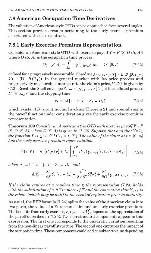
175
7.8 American Occupation Time DerivativesThe valuation of American-style OTDs can be approached from several angles.This section provides results pertaining to the early exercise premiumassociated with such a contract.
7.8.1 Early Exercise Premium RepresentationConsider an American-style OTD with exercise payoff Y = F (S, O (S, A))where O (S, A) is the occupation time process
(7.22)
defined for a progressively measurable, closed set . In the general market with Ito price process and
progressively measurable interest rate the claim’s price, Vt (Y), is given by(7.2). Recall the Snell envelope of the deflated process
and the stopping time
(7.23)
which exists, if D is continuous. Invoking Theorem 21 and specializing tothe payoff function under consideration gives the early exercise premiumrepresentation.
Theorem 100 Consider an American-style OTD with exercise payoff Y = F(S, O (S, A)) where O (S, A) is given in (7.22). Suppose that and that Y∈the function The value of the claim at t ∈ [0, τ0]has the early exercise premium representation
(7.24)
where and
(7.25)
If the claim expires at a random time τe the representation (7.24) holdswith the substitution of τe ^Τ in place of T and the convention that Yτe^Τ isthe rebate (which may be null) in the event of expiration prior to maturity.
As usual, the EEP formula (7.24) splits the value of the American claim intotwo parts, the value of a European claim and an early exercise premium.The benefits from early exercise, , depend on the appreciation ofthe payoff described in (7.25). Two non-standard components appear in thisexpression. The first one corresponds to the quadratic variation resultingfrom the non-linear payoff structure. The second one captures the impact ofthe occupation time. These components could add or subtract value depending
7.8. AMERICAN OCCUPATION TIME DERIVATIVES
© 2006 by Taylor & Francis Group, LLC
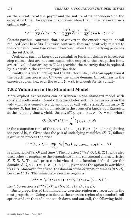
176 CHAPTER 7. OCCUPATION TIME DERIVATIVES
on the curvature of the payoff and the nature of its dependence on theoccupation time. The expressions obtained show that immediate exercise isoptimal only if
Ceteris paribus, contracts that are convex in the exercise region, entailreduced local benefits. Likewise contracts that are positively related tothe occupation time lose value if exercised when the underlying price liesin the set A(s,ω).
Contracts, such as knock-out cumulative Parisian claims or knock-outstep claims, that are not continuous with respect to the occupation time,are still valued according to (7.24) provided the maturity date is replacedby τeΛΤ with τe the random expiration date.
Finally, it is worth noting that the EEP formula (7.24) can apply even ifthe payoff function is not C2,1 over the whole domain. Smoothness in theexercise region, i.e., over the event {τs = s}, is enough for its validity.
7.8.2 Valuation in the Standard ModelMore explicit expressions can be written in the standard model withconstant coefficients r, δ and σ (Black-Scholes setting). Let us focus on thevaluation of a cumulative down-and-out call with strike K, maturity T,window D, barrier L and null rebate in the event of a knock-out. Exercise,at the stopping time τ, yields the payoff where
is the occupation time of the set duringthe period [0, τ]. Given that the pair of underlying variables, (S, O), followsa diffusion process the price
is a function of (S, O) and time t. The notation Ccdo(S, O, t; K, T, D, L) is alsoused below to emphasize the dependence on the contractual characteristicsK, T, D, L. The call price can be viewed as a function defined over thedomain , given that the option is worthlessif O ≥ D. Moreover, for t fixed, the domain of the occupation time is [0,t^d],because Ot ≤ t. The immediate exercise region is
Its (t, O)-section is Basic properties of the immediate exercise region are recorded in the
next proposition. Using ε to denote the exercise region of a standard calloption and εdoc that of a one-touch down-and-out call, the following holds
© 2006 by Taylor & Francis Group, LLC

177
Proposition 101 The immediate exercise region has the properties
(i) implies for all t ∈ [0, T] and s ∈ [t, T].(ii) implies ,
D/O > �2 = 1 and t ∈ [0, T].(iii) Suppose S < max
and ∈ [0, t^D].(iv) if and only if S ≥ K.(v) .
Properties (i)–(iv) are standard and parallel those for standard optionsstated in Proposition 31. The main difference pertains to the fact that theexercise region is defined in terms of a triplet (S, O, t), reflecting thedependence on the occupation time O. Property (ii) identifies the basicnature of this relation. It shows that the exercise region is connected, upto the boundary of the domain, in the O-direction. The reason for this featureis the negative impact of the occupation time on the option value. When theoccupation time increases the probability of an early knock-out increases,thereby reducing value. Immediate exercise is therefore optimal if it is optimalat the outset, i.e., at (S, O, t).
Property (v) shows the relations between the exercise regions associatedwith the one-touch down-and-out call, the cumulative barrier call and thestandard call option. The inclusions reported reflect the ordering of prices
American down-and-out calls are naturally worth less than standard calloptions that are not subject to knock-out prior to maturity. The Americancumulative down-and-out call is also worth more than the one-touch down-and-out call because of its resilience to breaches of the barrier: the optionremains alive at the first time at which the underlying price reaches thebarrier. The ordering of prices implies the ordering of the exercise regions.If immediate exercise is optimal for the plain vanilla call, it must also beoptimal for the two barrier options. Similarly, if it is optimal to exercisethe cumulative down-and-out call it is also optimal to exercise the one-touch barrier call.
The results of Proposition 101 enable us to define the boundary of theexercise region as where
is the smallest asset price in the exercise region at date t when the occupationtime is O. Moreover, standard arguments can be invoked to show that B (t,O) is a right-continuous, non-increasing function with respect to time. Fromproperty (ii) above it also follows that B (t, O) is non-increasing with respectto the occupation time. Limiting values can be also be easily inferred. As thematurity date approaches the likelihood of a knock-out goes to zero and theexercise region converges to that of a vanilla option. If t ≥ D and the
7.8. AMERICAN OCCUPATION TIME DERIVATIVES
© 2006 by Taylor & Francis Group, LLC

178 CHAPTER 7. OCCUPATION TIME DERIVATIVES
occupation time approaches the window the likelihood of a knock-out increases.In the limit (i.e., when O is very close to D, but strictly less) the cumulativebarrier option becomes similar to a newly issued one-touch option that isknocked out at the next touch of the barrier. The difference between the exerciseregions of the two options vanishes.
The definition of B (t, O) shows that immediate exercise is optimal whenS ≥B (t, O). The exercise region can be written as
and the event {τs = s} is the same as {Ss ≥ B (s, Os)}. The EEP formula inTheorem 100 takes the more explicit form
Theorem 102 Suppose that the underlying asset price follows the geometricBrownian motion process (4.1) and that the interest rate is constant. Thevalue of an American-style cumulative down-and out call has the earlyexercise premium representation
(7.26)
for represents the Europeancumulative call option value and πcdo(S, O, t, B(.)) is the early exercisepremium. These functions are given by
(7.27)
(7.28)
with log(y/S) /σ. The immediate exercise boundary Bcdoc solves the recursivenonlinear integral equation
(7.29)
for subject to the boundary conditions
(7.30)
(7.31)
At maturity BT=K≤BT-.
The EEP formula (7.26)–(7.28) identifies two value components embeddedin the price of an American cumulative down-and-out call. The first is thevalue of the European cumulative down-and-out call with identicalcharacteristics (K, T, D, L). The second is the value accruing from earlyexercise, prior to the minimum of the knock-out time and the maturitydate. Both value components are written in terms of the joint density
© 2006 by Taylor & Francis Group, LLC

179
function, defined in section 7.6.2, for the occupation time and the cumulativecontinuously compounded asset return per unit volatility.
The exercise premium component shows that value is created bycollecting the local benefits when immediate exercise is optimal and theknock-out provision is inactive. The innermost integral in (7.28) adds upthose benefits for prices above the exercise boundary B (s, O + v), conditionalon a fixed time s and a fixed occupation time v. The middle integral sumsup the cumulative benefits obtained over possible values of the occupationtime, conditional on a fixed time s. The outer integral adds up the twicecumulated benefits over times up to the maturity date. The order ofintegration is dictated by the dependence of the exercise boundary on theoccupation time. This can be contrasted with the European price (7.27)where the order of integration is immaterial.
As usual the EEP formula is parametrized by the exercise boundaryBcdoc, which, in this case, is a two dimensional surface depending on timeand on the value of the occupation time. Given that the formula holds forall values of (S, O, t) ∈ D, it holds on the boundary of the exercise region.This gives the integral equation (7.29). This equation, along with theboundary conditions (7.30)–(7.31), can in principle be used as the basis fora numerical scheme designed to compute the option value.
The transformations employed to derive the pricing expression inTheorem 102 can be carried out for several other occupation timederivatives. Cases requiring modifications of the results in Theorems 100and 102 are those where the dependence on the occupation time takes amore complex form than (7.22).
7.9 Multiasset ClaimsOccupation time derivatives can be easily generalized to the multiassetcase. For a progressively measurable, closed set A and an n-dimensionalvector of asset price processes S, a multiasset occupation time F-claim haspayoff F(S, K, OS,A) where
As before K represents a parameter such as a strike or a cap, dependingon the specific context.
7.9.1 Symmetry PropertiesMultiasset occupation time derivatives also satisfy certain symmetryproperties. To state the main result, recall the scaling operator in Appendix
defined for a constant � and a vector of prices S (the jth component of the pricevector is rescaled by the factor �). Also for a given occupation time F- claim
7.9. MULTIASSET CLAIMS
© 2006 by Taylor & Francis Group, LLC
A of chapter 6,

180 CHAPTER 7. OCCUPATION TIME DERIVATIVES
with parameter K and for any j = 1, …, n define the associated Fj-claimobtained by permutation of the jth argument and the parameter
with �j =K/Sj. With this notation the following natural generalization ofTheorem 95 is obtained.
Theorem 103 Consider an American-style occupation time F-claim withmaturity date T and a payoff function F(S, K, OS,A) which is homogeneousof degree one in (S, K). Let V(S, K, OS,A, r, δ; Ft) denote the value of the claimin the financial market with filtration F(.), asset prices S satisfying (2.26)and progressively measurable interest rate r. Pick some arbitrary index jand define
Prior to exercise the value of the multiasset occupation time F-claim is
where with
and . Here is thevalue of the Fj-claim with parameter , maturity date T andoccupation time in an auxiliary financial market with interest rateδj and in which the underlying asset prices follow the Ito processes
with respective initial conditions Si for i � j and K for i=j. The n-dimensionalprocess zj* is defined by
for all . The optimal exercise time for the occupation timeF-claim is the same as the optimal exercise time for the occupation time Fj
-claim in the auxiliary financial market.
The major difference relative to the single asset case is the choice ofnumeraire associated with the multidimensionality of the relevantvariables. Selecting a specific asset as the numeraire leads to one particularsymmetric contract. Another choice can produce a very different symmetricpayoff. In the end, all these contracts are related as they are derived froma common specification.
© 2006 by Taylor & Francis Group, LLC
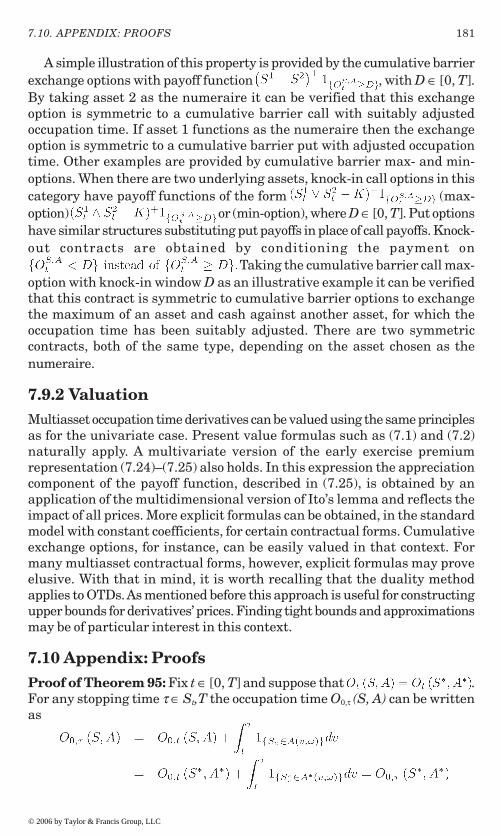
181
A simple illustration of this property is provided by the cumulative barrierexchange options with payoff function , with D ∈ [0, T].By taking asset 2 as the numeraire it can be verified that this exchangeoption is symmetric to a cumulative barrier call with suitably adjustedoccupation time. If asset 1 functions as the numeraire then the exchangeoption is symmetric to a cumulative barrier put with adjusted occupationtime. Other examples are provided by cumulative barrier max- and min-options. When there are two underlying assets, knock-in call options in thiscategory have payoff functions of the form (max-option) or (min-option), where D ∈ [0, T]. Put optionshave similar structures substituting put payoffs in place of call payoffs. Knock-out contracts are obtained by conditioning the payment on
Taking the cumulative barrier call max-option with knock-in window D as an illustrative example it can be verifiedthat this contract is symmetric to cumulative barrier options to exchangethe maximum of an asset and cash against another asset, for which theoccupation time has been suitably adjusted. There are two symmetriccontracts, both of the same type, depending on the asset chosen as thenumeraire.
7.9.2 ValuationMultiasset occupation time derivatives can be valued using the same principlesas for the univariate case. Present value formulas such as (7.1) and (7.2)naturally apply. A multivariate version of the early exercise premiumrepresentation (7.24)–(7.25) also holds. In this expression the appreciationcomponent of the payoff function, described in (7.25), is obtained by anapplication of the multidimensional version of Ito’s lemma and reflects theimpact of all prices. More explicit formulas can be obtained, in the standardmodel with constant coefficients, for certain contractual forms. Cumulativeexchange options, for instance, can be easily valued in that context. Formany multiasset contractual forms, however, explicit formulas may proveelusive. With that in mind, it is worth recalling that the duality methodapplies to OTDs. As mentioned before this approach is useful for constructingupper bounds for derivatives’ prices. Finding tight bounds and approximationsmay be of particular interest in this context.
7.10 Appendix: ProofsProof of Theorem 95: Fix t ∈ [0, T] and suppose that .For any stopping time τ ∈ St,T the occupation time O0,τ (S, A) can be writtenas
7.10. APPENDIX: PROOFS
© 2006 by Taylor & Francis Group, LLC

182 CHAPTER 7. OCCUPATION TIME DERIVATIVES
where is the occupation time of therandom set A* by the process S*. Performing the usual change of measureleads to the result stated. �
Proof of Theorem 96: The proof of the theorem relies on the next 3lemmas. Throughout it is assumed that the uncertainty is generated by aBrownian motion z~. A progressively measurable process is understood tobe adapted to the Brownian filtration.
Lemma 104 Let Z be a progressively measurable, continuous process withα-quantile Mz (α, t) and define the transformed process S = f (Z) where f(.) :D→D+ is a continuous and increasing function. The α-quantile of S is thetransform of the α-quantile of Z, that is M (α,t)=f(MZ(α,t)).
Proof of Lemma 104: The definition of an α-quantile and the properties ofthe map f give
The equality on the second line uses the fact that f is increasing and continuous.The third line follows from the definition x = f(y). The expression obtainedrepresents a constrained minimization problem (of the function f(y)) subject toa constraint on y. For the fourth line note that the function f (�) is strictlyincreasing: the minimization can then be performed directly over the argumenty. The last line is the definition of the α-quantile of Z. �
Lemma 105 Let Z be α progressively measurable, continuous process withZ0 = 0 and a-quantile Mz (α, T) over the interval [0, T]. Then
where
and is the α-quantile of the process Z in the
interval [t, T].
© 2006 by Taylor & Francis Group, LLC
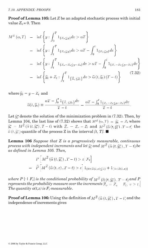
183
where and
Let denote the solution of the minimization problem in (7.32). Then, byLemma 104, the last line of (7.32) shows that where
with and thequantile of the process Z in the interval [t, T]. �
Lemma 106 Suppose that Z is a progressively measurable, continuousprocess with independent increments and let and beas defined in Lemma 105. Then,
where P [.| Ft] is the conditional probability of and Prepresents the probability measure over the increments The quantity α(t,z) is Ft-measurable.
Proof of Lemma 106: Using the definition of and theindependence of increments gives
Proof of Lemma 105: Let Z be an adapted stochastic process with initialvalue Z0 = 0. Then
(7.32)
7.10. APPENDIX: PROOFS
© 2006 by Taylor & Francis Group, LLC
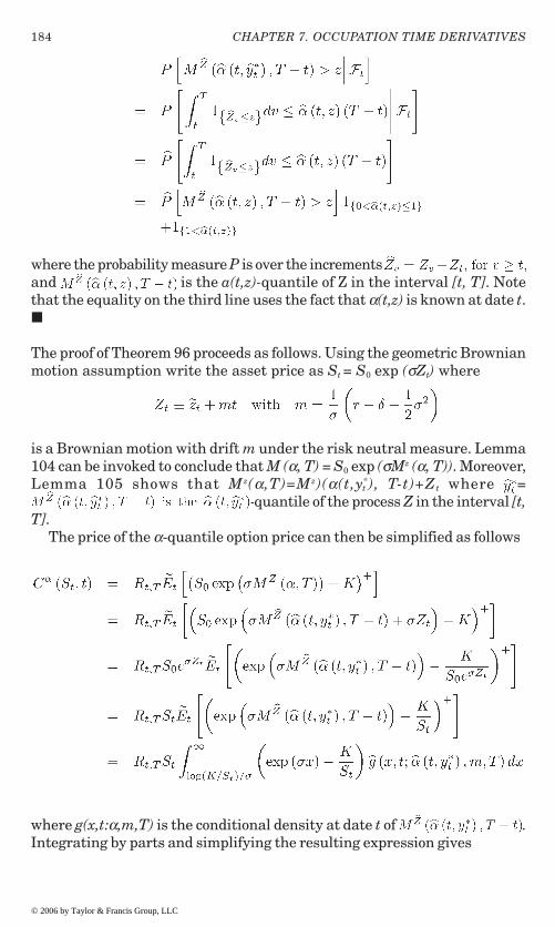
184 CHAPTER 7. OCCUPATION TIME DERIVATIVES
where the probability measure P is over the increments and is the a(t,z)-quantile of Z in the interval [t, T]. Notethat the equality on the third line uses the fact that α(t,z) is known at date t.�
The proof of Theorem 96 proceeds as follows. Using the geometric Brownianmotion assumption write the asset price as St = S0 exp (σZt) where
is a Brownian motion with drift m under the risk neutral measure. Lemma104 can be invoked to conclude that M (α, T) = S0 exp (σMz (α, T)). Moreover,Lemma 105 shows that Mz(α,T)=Mz)(α(t,yt
*), T-t)+Zt where =quantile of the process Z in the interval [t,
T].The price of the α-quantile option price can then be simplified as follows
where g(x,t:α,m,T) is the conditional density at date t of .Integrating by parts and simplifying the resulting expression gives
© 2006 by Taylor & Francis Group, LLC
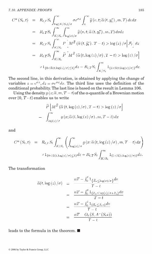
185
The second line, in this derivation, is obtained by applying the change ofvariables The third line uses the definition of theconditional probability. The last line is based on the result in Lemma 106.
Using the density of the α-quantile of a Brownian motionover [0, T - t] enables us to write
and
The transformation
leads to the formula in the theorem. �
7.10. APPENDIX: PROOFS
© 2006 by Taylor & Francis Group, LLC

186 CHAPTER 7. OCCUPATION TIME DERIVATIVES
Proof of Theorem 98: The arguments following the theorem show that
where
To complete the proof it remains to characterize the function hl (T, y). Thisis accomplished in the next lemma which gives the Laplace transform ofhl (T, y). �
Lemma 107 (Chesney, Jeanblanc-Picque and Yor [1997]) The function hl (T,y) has Laplace transform dt given by
In the special case y > l the Laplace transform simplifies to
section 5 and Appendix. �
Remark 7 A more explicit expression for Kλ,D(a) can be obtained byperforming the integration. This gives
where dx is the density of the first hittingtime of the level l by a Brownian motion and
if l >0.
if l <0
© 2006 by Taylor & Francis Group, LLC
Proof of Lemma 107: See Chesney, Jeanblanc-Picque and Yor [1997],

187
with
The following expression for the function (T,d,D,l) in section 7.6.3 isprovided by Hugonnier [1999] and Moraux [2002].
Lemma 108 (Hugonnier [1999], Moraux [2002]) For S < L (or l > 0),
(7.33)
For S > L (or l < 0) it holds that
(7.34)
with
(7.35)
and
(7.36)
(7.37)
Similar formulas can be established for .
Proof of Lemma 108: Assume 0 < D < T and recall that
7.10. APPENDIX: PROOFS
© 2006 by Taylor & Francis Group, LLC
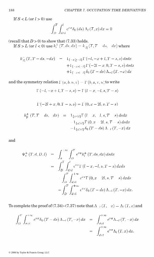
188 CHAPTER 7. OCCUPATION TIME DERIVATIVES
If S < L (or l > 0) use
(recall that D > 0) to show that (7.33) holds.If S > L (or l < 0) use where
and the symmetry relation to write
and
To complete the proof of (7.34)–(7.37) note that and
© 2006 by Taylor & Francis Group, LLC

189
with and as defined in (7.36)–(7.37). �
Remark 8 The following explicit formula for the function Γ in (7.19) andLemma 108 is provided by Hugonnier [1999],
Following Moraux [2002] one can then show that
This expression, obtained by collecting terms and performing the integrationin (7.19), proves useful for the implementation of the valuation formulas forcumulative barrier claims.
Proof of Theorem 100: The EEP representation in (7.24) follows immediatelyfrom Theorem 21. The appreciation component (7.25) of the payoff Y = F (S,O) is obtained by an application of Ito’s lemma. This derivation uses theevolution equation for the occupation time, �
Proof of Proposition 101: Properties (i), (iii) and (iv) are natural extensionsof similar properties for vanilla options, and are proved along the same lines.For property (ii) note that
7.10. APPENDIX: PROOFS
© 2006 by Taylor & Francis Group, LLC

190 CHAPTER 7. OCCUPATION TIME DERIVATIVES
A standard argument can then be invoked to prove the claim. Property (v)follows from the bounds
where the contractual characteristics associated with the options involvedhave been specified. Assume that the down-and-out options are alive. It isthen clear that the optimality of immediate exercise of the vanilla callimplies the optimality of immediate exercise of the two knock-out options(otherwise immediate exercise cannot be optimal for the vanilla option).Likewise, optimality of immediate exercise for the cumulative knock-outcall implies optimality of immediate exercise for the standard knock-outcall. The ordering of exercise regions follows. �
Proof of Theorem 102: For a cumulative down-and-out call the EEPformula in Theorem 100 becomes
with
and .The European option value can be simplified using the additivity of the
occupation time and the change of measure
described in section 7.5. This gives
In the equality on the first line Ot,T is the occupation time of the set A- (L)during the period [t, T] and the conditional expectation is over the joint
© 2006 by Taylor & Francis Group, LLC

191
distribution of ZT - Zt and Ot,T. The equality on the second line integrates overthe bivariate law of ZT - Zt and Ot,T. The next expression is obtained byrestricting the second integral to the domain over which the indicator functionis one. The final formula restricts the first integral to the domain over whichthe option payoff is positive.
Similar transformations can be performed to simplify the exercisepremium component. Using the equality of events
where B (s, Os) is the exercise boundary at dates and simplifying the resulting expression gives
where
The steps in this derivation are, by now, standard. The only noteworthyaspect is the fact that the outside integral in the final expression for φ (S,O,s–t) is over the occupation time v during the period [t, s], whereas the insideintegral is over values of x for which immediate exercise at s is optimal. Thisorder of integration is dictated by the dependence of the exercise boundary B(s, O + v) on the occupation time v.
The recursive equation for the exercise boundary follows immediatelyfrom the EEP representation formula. The boundary conditions arediscussed in the text preceding the theorem. �
Proof of Theorem 103: Fix a time t and suppose that asset j is selectedas the numeraire. By the homogeneity property the payoff function can berescaled and rewritten as
7.10. APPENDIX: PROOFS
© 2006 by Taylor & Francis Group, LLC
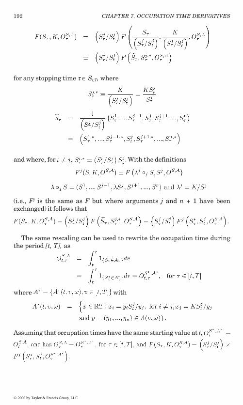
192 CHAPTER 7. OCCUPATION TIME DERIVATIVES
and where, for With the definitions
(i.e., Fj is the same as F but where arguments j and n + 1 have beenexchanged) it follows that
The same rescaling can be used to rewrite the occupation time duringthe period [t, T], as
where with
for any stopping time τ ∈ St,T, where
Assuming that occupation times have the same starting value at t,
© 2006 by Taylor & Francis Group, LLC

193
With this notation the price of the American multiasset OTD is
where is the discount factor based on the rate δ and is the conditional expectation at t based on the measure
The last expression is the value at time t of an American OTD with payofffunction Fj, written on the price vector S*, with fixed parameter andoccupation time Os*,A, in an economy with interest rate equal to δ. It can beverified that the evolution of S* in the modified economy is described bythe equations reported in the theorem. Asset j, therefore, has dividendyield r while asset i’s dividend yield remains the same. The vector ofdividend rates can be written as , as stated. �
7.10. APPENDIX: PROOFS
© 2006 by Taylor & Francis Group, LLC

195
Chapter 8
Numerical Methods
This chapter presents numerical methods developed to compute the optimalexercise boundary and the value of an American option. Particular emphasisis placed on recent approaches. Our presentation starts with a briefsummary of popular methods proposed during the last three decades(section 8.1). Approaches based on the integral equation for the boundary(section 8.2) and on simple approximations of the optimal exercise policy(section 8.3) are reviewed next. Both of these sections assume that theunderlying asset price is a geometric Brownian motion process and thatthe interest rate is constant. Extensions to more general diffusions (section8.4) and a summary of additional recent methodologies follow (section 8.5).A numerical study is carried out to compare the efficiencies of some of theapproaches described (section 8.6). A presentation of methods for multiassetoptions (section 8.7) and for occupation time derivatives (section 8.8)concludes the chapter.
8.1 Numerical Methods for American OptionsAs shown in the previous chapters there is no known simple analyticformula for pricing an American option. As a result one must eventuallyresort to a numerical method to compute the value of a given contract. Anumber of approaches have been proposed for that purpose. Among themajor ones we find computational methods based on lattices, partialdifferential equations, variational inequalities, integral equations, stoppingtime approximations and Monte Carlo simulation. In this section we brieflysurvey the first three approaches and the related literature. Other methodswill be presented in more details in the following sections.
Lattice methods are among the oldest approaches pursued and perhapsthe simplest ones. They rely on the fact that a geometric Brownian motionprocess can be approximated by a binomial lattice and that the resultingoption price constitutes an approximation of the true price. The advantageof a latticebased approach is that it reduces an infinite dimensional problemto a finite dimensional one. This is accomplished by discretizing the timeinterval into a finite number of subintervals, n, and assuming that the
© 2006 by Taylor & Francis Group, LLC

196 CHAPTER 8. NUMERICAL METHODS
underlying asset price has only a finite number of outcomes at each node ofthe tree. The most common lattice approach, the binomial method, postulatesan asset price with two possible outcomes at each node (Su, Sd) where u(resp. d) is the gross return if the price goes up (resp. down). Thus, each nodeof the tree has two follower nodes. If u, d are constants the tree is said to berecombining. In this case the total number of nodes at step j is j + 1, j = 1, …,n. The American option price can then be easily computed in a backwardmanner starting from the last step, n (the maturity date). At that point theoption value is the exercise value. So, for a call option
for i = 0, …, n. At step n - 1 there are n nodes, andtherefore n option values. These are computed using risk neutral valuation.Thus,
for i = 0, …, n - 1, where isthe continuation value, is the immediate exercise value andq the risk neutral probability. At step j there are j + 1 prices to compute, that areobtained using the same formula (replacing n - 1 by j). The option price at theinitial date (with one node) is the unique value obtained at that point. Theoptimal exercise policy is the first time at which immediate exercise is optimal
. The optimal exerciseboundary is where
This simple approach was initiated by Cox, Ross and Rubinstein [1979].A variant of the method uses a trinomial lattice, with three follower nodesissued from each node of the tree, to compute prices. This modificationwas proposed by Parkinson [1977] and Boyle [1988] and is analyzed byOmberg [1988]. Additional refinements of the binomial approach andimprovements in its implementation can be found in Rendleman andBartter [1979], Jarrow and Rudd [1983], Hull and White [1988], Amin[1991], Trigeorgis [1991], Tian [1993], Kim and Byun [1994], Leisen andReimer [1995] and Curran [1995]. A proof of convergence for lattice methodsappears in Amin and Khanna [1994]. The convergence of the optimalexercise boundary is proved by Lamberton [1993]. Convergence rates forEuropean-style options are derived in Leisen and Reimer [1995]. For thosecontracts Diener and Diener [2004] carry out a detailed asymptotic analysisof the behavior of the binomial approximation. Numerical estimates ofconvergence rates for American-style option prices appear in Broadie andDetemple [1996]. Analytical bounds for convergence rates of Americanoption prices in binomial lattices are derived by Lamberton [1998].1
Partial differential equations methods rely on the fundamental valuationequation derived by Black and Scholes [1993] and Merton [1993]. This
1The price of an American contingent claim can also be estimated by using a randomwalk approximation of the underlying Brownian motion. Error estimates for these types ofapproximations are provided by Lamberton [2002].
© 2006 by Taylor & Francis Group, LLC

197
equation states that an American call option price C(S, t) satisfies
subject to the boundary conditions Here Ct, Cs and Css are
the partial derivatives with respect to time t and the price S. Finite differencemethods to solve this equation were introduced by Schwartz [1977] andBrennan and Schwartz [1977, 1978]. Convergence of the Brennan andSchwartz algorithm is proved in Jaillet, Lamberton and Lapeyre [1990] andZhang [1995]. Related numerical methods can be found in Courtadon [1982]and Hull and White [1990]. Some authors have also proposed approximationsof the fundamental valuation PDE that admit closed form solutions. Thequadratic method of MacMillan [1986] and Barone-Adesi and Whaley [1987],as well as the method of lines of Carr and Faguet [1995], fall in that category.
An approximation that echoes some features of the binomial latticeconstruction is the one proposed by Geske and Johnson [1984]. Thisapproach discretizes the time interval into n subintervals and evaluatesthe American option price as a multidimensional integral involving therelevant payoffs at each discretization point. In effect the method uses anapproximation of the true price corresponding to an exercise policyrestricted to the n discretization points selected. Implementation of theformula requires numerical approximations of the multidimensional integralsand of the exercise boundary. Geske and Johnson [1984] also introduceRichardson extrapolation in the context of option pricing. This extrapolationtechnique has proved popular and is also used by Breen [1991], Bunch andJohnson [1992], Ho, Stapleton and Subrahmanyam [1994], Huang,Subrahmanyam and Yu [1996] and Carr and Faguet [1995]. For a full
The variational inequality approach to option pricing was introducedby Jaillet, Lamberton and Lapeyre [1990]. A discretization of the relevantvariational inequality leads to a linear complementarity problem that can
[1992]). An overview of PDE and variational inequality approaches isprovided in the textbook of Wilmott, Dewyne and Howison [1993]. A shortsurvey can be found in Broadie and Detemple [2004].
8.2 Integral Equation MethodsIntegral equation methods are based on the EEP representation formulafor the option price and the associated integral equation for the exerciseboundary. The numerical implementation procedure suggested by thisformula involves two steps. The first step consists in computing the optimalexercise boundary B, the second step in computing the option price takingthe curve B as an input.
Implementation of this procedure starts with the equation for the optimalexercise boundary. Let us focus on the case of a call option with strike K
8.2. INTEGRAL EQUATION METHODS
© 2006 by Taylor & Francis Group, LLC
treatment of Richardson extrapolation see Marchuk and Shaidurov [1983].
be solved by linear programming methods (see Cottle, Pang and Stone

198 CHAPTER 8. NUMERICAL METHODS
and maturity date T. For the standard market model we know, from chapter4, that the optimal exercise boundary B of this option solves the equation
(8.1)
where c(Bt, t) is the European option value evaluated at St = Bt and
with
subject to the terminal condition BT- = K max{1, r/δ }. This is a backward equation,which naturally suggests a recursive algorithm to compute its solution.
The algorithm works as follows. Divide the period [0, T] into n equalsubintervals and let Δt =T/n. For j = 0, …, n set t(j) = jΔt. We seek a step
function approximation that can be computed
recursively. Step function approximations have been suggested by Huang,Subrahmanyam and Yu [1996].
From the terminal condition we have B(n) (n)= K max(1, r/δ ). Supposenow that B(n)(l) is known for all l > j. A non-linear equation for B(n) (j),parametrized by {B(n) (l) l = j + 1,…,n}, is obtained by discretizing the integralon the right hand side of (8.1). This can be done in several ways by usingdifferent quadrature approximations of the integral. If we use the trapezoidal
equation
(8.2)
with unknown B(n)(j). Its solution B(n)(j) can be computed using an iterativemethod. This produces an approximation of the boundary at time t(j). Repeatingthis computation recursively from j = n - 1 to 0 yields a step functionapproximation of the exercise boundary, .
Several iterative methods are available to compute the solution of (8.2) ateach step j. Kallast and Kivinukk [2003] have recently proposed to use the
© 2006 by Taylor & Francis Group, LLC
rule (see Press, Teukolsky, Vetterling and Flannery [1992]) we obtain the

199
Newton-Raphson procedure and shown that it has good efficiency properties.2
Let F (B(n)(j)) denote the difference between the left and the right hand sidesof (8.2). The Newton-Raphson scheme produces a sequence of approximations{B(n,k) (j) : k = 0, 1, 2…} at step j according to the map
where F’(x) is the derivative of F(x). The initial value of the sequence can beselected as The scheme is run until the differencebetween successive iterates falls below some selected tolerance level �. When
the next iterate decreases (i.e., because When it increases. In numericalexperiments this scheme converges, and does so quickly.
The algorithm described above produces an approximate exerciseboundary, hence an approximate option value, for any fixed number oftime steps n. The true price is the limit as n goes to infinity. As computationsare based on finite discretizations of the time interval one may want toimprove efficiency for a given selection n. This can be achieved by usingthe standard Richardson extrapolation scheme that gives theapproximation where C(n) (S, t) is theapproximate price with n discretization points. Alternative extrapolationschemes, such as the one proposed by Geske and Johnson [1984], statingthat can also beemployed to that effect.
8.3 Exercise Time Approximations: LBA-LUBAThe approximations presented in the previous section are constructeddirectly from the recursive equation characterizing the optimal exerciseboundary. An alternative approach is to restrict attention to a class ofexercise policies that are easy to evaluate and to choose the best one withinthis class. This is the key idea behind the procedure proposed by Broadieand Detemple [1996]. Their approach produces a lower bound for theexercise boundary, lower and upper bounds for the option price andapproximate option values that are called lower bound approximation (LBA)and lower-upper bound approximation (LUBA).
8.3.1 A Lower Bound for the Option Price
A particularly simple exercise policy consists in exercising at the first hittingtime of a prespecified constant level L, or at maturity if this event does notmaterialize before the expiration date of the contract. This policy isrepresented by the stopping time
if no such time exists in [t,T]
2 Ju [1998] uses a two-dimensional Newton-Raphson scheme to solve for the freeparameters in an exponential approximation of the boundary (see section 8.5.2).
8.3. EXERCISE TIME APPROXIMATIONS: LBA-LUBA
© 2006 by Taylor & Francis Group, LLC

200 CHAPTER 8. NUMERICAL METHODS
This policy is certainly feasible for the holder of an American option that allowsfor unrestricted exercise time. Thus, our class of simple stopping times is
Implementation of a stopping time gives the payoff of acapped option with automatic exercise at the cap L. Suppose that we hold anAmerican call with strike K and maturity date T. In this case the exercise policy�L has a value equal to C (S, t; L), the price of a capped call option with strike K,maturity date T and automatic exercise at the cap L. As �L is feasible for theAmerican call the lower bound C (S, t) � C (S, t, L) holds, and this for any L �0. Given that the capped option is automatically exercised at L=S we can restrictattention to constants L � S. Let be the correspondingclass of stopping times. Maximization with respect to these exercise policiesproduces the highest lower bound3
As the price C(S, t; L) is available in closed form this optimization can beperformed using standard iterative methods (such as Newton-Raphson).
8.3.2 A Lower Bound for the Exercise Boundary
The lower bound for the American option price derived above can be usedto construct a lower bound for the optimal exercise boundary. To derivethis bound define
(8.3)
which represents the derivative of the capped call with respect to the cap,evaluated at the point where the cap equals the asset price, i.e., L = S.When D(S, t) > 0 at a point S immediate exercise is suboptimal. Let
. This quantity is the smallest price at which immediateexercise is optimal when the option holder is restricted to policies of theform �L. Solving this optimization problem for t ∈ [0, T) produces a curve
. Basic intuition might suggest that L* is a lower boundfor the optimal exercise boundary B. This is indeed the case.
Proposition 109 Suppose that the underlying asset price satisfies (2.2). LetB be the optimal exercise boundary for the American call option, and L* thecurve solving for all t ∈ [0, T). Then
Moreover, and
3Similar ideas can also be found in Bjerksund and Stensland [1992] and Omberg [1987].
© 2006 by Taylor & Francis Group, LLC

201
The intuition underlying the lower bound is simple. Given that barrier policiestL are always feasible for the American call option it must be that immediateexercise is optimal for the capped option whenever it is optimal for the uncappedoption. This implies that the derivative D(S, t) � 0 when(S, t) ∈ ε. Taking the lowest price at which this slope is non-positive (i.e., L*
t = inf{S:D(S, t) � 0}) will then give a lower bound for the exercise boundary Bt (i.e.,L*
t �Bt ).The lower bound L* obtained via this procedure is very tight. As stated in
the proposition, it coincides with the immediate exercise boundary B at thematurity date T– and at very long maturities T – t → ∞. As shown in Figure8.1 the difference between the two curves is small at intermediate times.
Figure 8.1: This figure illustrates the difference between the immediate exerciseboundary B and its lower bound approximation L*. The boundary B is computedusing the integral equation. Parameter values are K = 100, r = δ = 0.06, σ = 0.2.Both curves are calculated using 100 time steps.
8.3.3 An Upper Bound for the Option Price
In turn, the lower bound for the boundary can be used to produce an upperbound for the American option price. Substituting the lower bound L*
t in place
8.3. EXERCISE TIME APPROXIMATIONS: LBA-LUBA
© 2006 by Taylor & Francis Group, LLC

202 CHAPTER 8. NUMERICAL METHODS
of Bt in the EEP formula gives the function
This function depends parametrically on the curve L*. It is easy to computeonce L* is known as it only depends on the cumulative normal distributionsappearing in c (S, t) and Our next proposition shows that itis an upper bound for the price.
Proposition 110 The American call option price is bounded above by the functionCu (S, t). Hence
Intuition for the upper bound can also be gathered by recalling that theearly exercise premium is given by the present value formula
Given that (from Proposition 109) we see that the net
benefits of exercising, δ Ss - rK, are positive over the event {Ss � L*s}, and
this for all s ∈ [0, T]. Substituting this event in place of {Ss � Bs} in thepremium and using the inclusion {Ss � Bs} � {Ss � L*
s} produces an upperbound. This upper bound corresponds to the function Cu (S, t) defined above.
8.3.4 Price Approximations
The bounds Cu, Cl can be used to construct various approximations of theAmerican call option. For example the weighted sums
are suggested by Broadie and Detemple [1996]. The estimate C1(S, t) is alower bound approximation (LBA) of the American option price; C2(S, t) is alower-upper bound approximation (LUBA). They report that simple choicesof the weights (e.g., �1 = 1 and �2 = 0.5) already provide good results in typicalsituations. Better weights can be obtained by using a regression approachbased on a sample of parameter configurations. Nonparametric methodscould also be employed to capture non-linearities in these relationships.
8.4 Diffusion ProcessesThe computational procedures presented in the previous sections can alsobe applied in more general diffusion settings. Specifically, suppose thatthe underlying asset price follows the risk neutralized process
(8.4)
© 2006 by Taylor & Francis Group, LLC

203
where r (S, t) is the interest rate, σ (S, t) the return volatility, δ (S, t) thedividend yield and a Brownian motion under the risk neutral measure(the setting of section 4.6). As before assume that the coefficients r (S, t), σ(S, t), (δ (S, t) are continuously differentiable and satisfy suitable conditionsfor the existence of a solution to this stochastic differential equation, thatσ (S, t) is positive and that r (S, t) is a decreasing function of S and anincreasing function of t, while δ (S, t) S is an increasing function of S. Alsoassume decreasing timemonotonicity. In the remainder of this section weshow how to adapt integral equation and stopping time approximationmethods to handle this setting.
8.4.1 Integral Equation Methods
Under the conditions of the model we know that the optimal exercise boundaryis unique and satisfies the recursive integral equation (4.11) subject to theappropriate boundary condition. This equation can be simplified if thetruncated moments in the integral equation can be written more explicitly,in terms of known density and cumulative distribution functions. In thiscase the exercise boundary B of a call option satisfies
where the functions c (B(t), t) and φ (Β (t), t; B(v), v) involve the relevantdensity and distribution functions. This integral equation is subject to theterminal condition B(T–) = K V B* where B* solves the nonlinear equation
if an interior solution exists. If for all possiblerealizations S of the process (8.4) at T set (the highest possible valueof S). If for all possible realizations S of the process(8.4) at T set (the lowest value of S). If an interior solution exists it isunique because r (S, T) is decreasing in S while δ (S, T) S is increasing.
This recursive integral equation has the same structure as (8.1), albeitwith a different integrand and a boundary condition thatinvolves the solution of a nonlinear equation. It is then clear that thenumerical algorithms described in section 8.2 can also be used in this case.
8.4.2 Stopping Time Approximations: LBA and LUBA
Likewise, the stopping time approximations in section 8.3 can be adapted tohandle the case of diffusion processes such as (8.4). In fact, the construction ofthe bounds is valid in the generality of this model, as it does not require theexistence of closed form expressions for distributions or truncated moments.
The construction of the bounds proceeds as in section 8.3. A lower pricebound is given by where C (S, t; L) is the
8.4. DIFFUSION PROCESSES
© 2006 by Taylor & Francis Group, LLC

204 CHAPTER 8. NUMERICAL METHODS
price of a capped call option with automatic exercise at the cap L, andsame strike K and maturity date T as the American call option to bepriced. A lower bound for the exercise boundary is given by the time-dependent function L*
t ≡ inf {S : D (St) � 0} where D (S, t) is defined as in(8.3). An upper price bound is then obtained by substituting L* in place ofB in the EEP formula. Proofs of these results can be found in Detempleand Tian [2002].
Therefore, all the elements of the LBA and LUBA algorithms extend togeneral diffusion processes satisfying the assumptions stated above.Although the construction does not require explicit distributions, thisapproach becomes particularly attractive when the capped call option priceC (S, t; L) has a closed form expression. In this case the computation of L*and of the price bounds is fast and easy to perform.
8.5 Other Recent Approaches
8.5.1 Lattice Methods: Binomial Black-Scholes Algorithm
A modification to the binomial lattice method was proposed by Broadie andDetemple [1996]. This approach is based on the usual binomial recursivealgorithm except that it replaces the continuation value at the last stepprior to maturity (i.e., step n - 1) by the Black-Sholes value. The approach istermed BBS (i.e., Binomial with Black-Scholes modification). The interestof this modification stems from its reduced error and smoother convergenceto the true value. Combining the procedure with Richardson extrapolationgives another approximation called BBSR (i.e., Binomial with Black-Scholesmodification and Richardson extrapolation). Broadie and Detemple [1996,1997b] show that BBS and BBSR perform significantly better than thestandard binomial lattice methods when efficiency is measured by the trade-off between computation speed and error. They also show that LBA andLUBA give even better results than BBS and BBSR. Their numerical resultsare generated using a sample of about 2, 500 randomly selectedconfigurations for the parameters of the option pricing model.
8.5.2 Integral Equation: Non-linear Approximations
Instead of using step functions in order to approximate the solution of theintegral equation one could employ piecewise non-linear functions. Ju[1998] proposes a multipiece exponential function. In his method theexercise boundary is approximated, within each subinterval, by anexponential function of time (e.g., Integration by parts can then be used to express the integral of thediscounted gains from exercise in terms of cumulative normal distributions.This gives an approximation of the recursive part of the integral equationthat involves a single integral, the one in the cumulative normaldistributions. A by-product is an approximation formula for the option value
© 2006 by Taylor & Francis Group, LLC

205
in terms of cumulative normals. Given that the exponential function has afree parameter bi, that must be estimated along with the boundary point ,the equation for the boundary is solved in conjunction with the smoothpasting condition. Performing this computation recursively gives amultipiece exponential estimate of the boundary. An estimate of the optionprice is then obtained from the approximate option pricing formula.
This scheme can be combined with Richardson extrapolation to improveefficiency. Ju shows that a 3-point extrapolation scheme (where the pointscorrespond to one, two and three subintervals) performs about as well asLUBA in terms of root mean square error and speed of computation. Thisresult is obtained using a sample of 1, 250 randomly generated optionparameter configurations.
8.5.3 Monte Carlo Simulation
Monte Carlo simulation has long been used for pricing European-stylederivative securities. The method was introduced in the field by Boyle[1977]; a detailed survey can be found in Boyle, Broadie and Glasserman[1997]. Attempts at applications to American-style securities are morerecent and were initiated by Tilley [1993], in the context of single assetmodels. The main difficulty in using simulation to price American claimsis the need to derive the optimal stopping rule in conjunction with theclaim’s price. The recursive nature of this optimization problem conflictswith the inherent forward looking structure of the simulation approach.Various approaches have been proposed to deal with this difficulty. Someof the recent contributions include Barraquand and Martineau [1995],Carriere [1996], Broadie and Glasserman [1997a], [1997b], Broadie,Glasserman and Jain [1997], Raymar and Zwecher [1997], Carr [1998]and Longstaff and Schwartz [1999]. Further developments, based on duality(see section 3.4), can be found in Rogers [2002], Haugh and Kogan [2004]and Andersen and Broadie [2004].
Monte Carlo simulation is especially useful for dealing with contingentclaims written on multiple underlying assets. Much of the recent literaturecited above, in fact, attempts to develop the simulation-based approach formultiasset derivatives. A description of the some of these developments isprovided in the last section of this chapter.
8.6 Performance EvaluationTo provide perspective on the numerical methods for univariate pricingproblems we conduct a numerical study designed to evaluate the relativeefficiencies of the methods presented. For parsimony we focus on theBinomial (B) algorithm, the Binomial-Black-Scholes (BBS) approach, theintegral equation (IE) method and the lower and upper boundapproximations (LBA and LUBA). Complementary results for additionalmethods can be found in Broadie and Detemple [1996], [1997b].
8.6. PERFORMANCE EVALUATION
© 2006 by Taylor & Francis Group, LLC
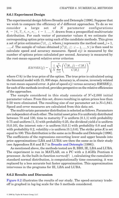
206 CHAPTER 8. NUMERICAL METHODS
8.6.1 Experiment Design
The experimental design follows Broadie and Detemple [1996]. Suppose thatwe wish to compare the efficiency of J different approaches. To do so weconsider a large set of N parameter configurations
drawn from a prespecified multivariatedistribution. For each vector of parameter values θi we estimate thecorresponding option price using each of the candidate methods. This givesa set of price estimates where j represents the method used, j = 1,…, J. The sample of values obtained is then used tocalculate speed and accuracy measures. Speed s(j) is measured by thenumber of options prices calculated per second. Accuracy is measured bythe root-mean-squared relative error criterion
where C(θi) is the true price of the option. The true price is calculated usingthe binomial model with 15, 000 steps. Accuracy is, of course, inversely relatedto root-mean-squared error. A plot of speed s(j) versus accuracy RMSRE(j),for each of the methods involved, provides perspective on the relative efficienciesof the approaches.
The sample considered in this study consists of N’=2,000 initialparameter values. From this set, draws resulting in option prices less than0.50 were eliminated. The resulting size of our parameter set is N=1,841.Speed and error measures are calculated from this data set.
The multivariate parameter distribution is selected as follows. Parametersare independent of each other. The initial asset price S is uniformly distributedbetween 70 and 130, time to maturity T is uniform [0.1,1] with probability0.75 and uniform [1, 5] with probability 0.25, the dividend yield d is uniform[0,0.10], the interest rate r is uniform [0,0.1] with probability 0.8 and nullwith probability 0.2, volatility s is uniform [0.1,0.6]. The strike price K is setequal to 100. This distribution is the same as in Broadie and Detemple [1996].The coefficients of the regressions converting lower and upper bounds intoprice approximations (LBA and LUBA) are then the same as in their study(see Appendices B.6 and B.7 in Broadie and Detemple [1996]).
As mentioned above, the methods tested are B, BBS, IE, LBA and LUBA.The experiment is run in MATLAB, on a PC with a 2.4GHz Pentium 4processor. As the built-in function normcdf (�), calculating the cumulativestandard normal distribution, is computationally time consuming, it wasreplaced by a less accurate but faster approximation. This approximationintervenes in the programs for IE, LBA and LUBA.
8.6.2 Results and Discussion
Figure 8.2 illustrates the results of our study. The speed-accuracy trade-off is graphed in log-log scale for the 5 methods considered.
© 2006 by Taylor & Francis Group, LLC

207
The version of the binomial algorithm tested uses the parametrizationproposed by Hull and White [1988]. The plot is for time discretizations of 25,50, 100, 200, 300, 400, 500, 600, 800, 1,000 and 1,200. The trade-off is clear:an increase in the number of time steps increases accuracy but also slowsdown computations. For n = 400 root-mean-squared relative error is about 6× 10⁻⁴ and computation speed about 2.4 × 10. BBS is tested using the sameparametrization of the tree (of course with Black-Scholes correction at thelast step). The plot is for time discretizations of 25, 50, 100, 200, 300, 400,500, 600 and 800 . The graph shows uniform dominance over the binomial:for any fixed accuracy level BBS calculates more options per second than B.
The integral equation method is tested for discretizations n = 4, 8 and16. The computation of the boundary approximation at each time step(i.e., the solution of the integral equation) is performed using a Newton-Raphson procedure. Strikingly, performance does not improve relative tothe binomial method. For the sample drawn B dominates IE when thetime discretization is 4 or 8, and performs about the same as IE with adiscretization of 16. Both B and IE are dominated by BBS over the rangeof discretizations studied. The lower slope of the trade-off for IE, though,indicates that its relative performance should improve as the number ofdiscretization points increases.
LBA and LUBA are also implemented using the Newton-Ralphsonalgorithm to solve the non-linear equations for the optimal barrier policies.LBA has an accuracy which is roughly of the order of 10-3 for a speed ofcomputation about equal to 3.4 × 10². LUBA reaches an accuracy of about2×10-4 for a speed in the neighborhood of 102. This represents animprovement over BBS by a factor of 10, and over B by a factor of 50.
These results are in line with those reported in Broadie and Detemple[1996], [1997b]. Broadly speaking they document the dominance of LBAand LUBA over the other candidate methods tested. BBS also exhibitsgood performance properties. Given the simple and intuitive nature of themethod it may be the approach of choice for non-specialists. One notabledifference is the slightly worse performance of IE. The small variationrecorded here could be due to differences in precision parameters selectedin the program and/or to differences in the implementation of built-infunctions across software platforms.
8.7 Methods for Multiasset OptionsThis section provides a brief overview of numerical methods that have beendeveloped to deal with multiasset options. We first survey lattice methods,then present more recent developments based on Monte Carlo simulation.
8.7.1 Lattice Methods
Multinomial lattice methods naturally extend the principles underlying thebinomial approach to option pricing. As for the latter, the central idea is to
8.7. METHODS FOR MULTIASSET OPTIONS
© 2006 by Taylor & Francis Group, LLC

208 CHAPTER 8. NUMERICAL METHODS
discretize the prices of the underlying assets and then to use a backwarddynamic programming algorithm to compute the option value. One of thenew challenges is to find a discretization that provides not only a gooddescription of the individual characteristics of assets but also of therelationships across prices. Various multinomial procedures have beenproposed to that effect. Some of the most prominent ones include Boyle [1988],Boyle, Evnine and Gibbs [1989], Madan, Milne and Shefrin [1989], Cheyette[1990], He [1990], Kamrad and Ritchken [1991] and Rubinstein [1994].
The approach proposed by Boyle, Evnine and Gibbs [1989] illustrates thebasic ingredients needed to deal with the multivariate case. Suppose that theobjective is to price an American claim written on k underlying assets. This canbe done by constructing an approximation of the price based on a lattice with 2k
branches issued from each node. For the two-asset case this gives 4 branchesleading to 4 pairs of outcomes and
Figure 8.2: This figure shows the efficiency of the Binomial method (B), the BinomialBlack-Scholes approach (BBS), the Integral Equation method (IE), the Lower BoundApproximation (LBA) and the Lower-Upper Bound Approximation (LUBA). Speedis measured in options per second (y-axis). Accuracy is measured by the root-mean-squared relative error (x-axis).
© 2006 by Taylor & Francis Group, LLC

209
(S1 d1, S2 d2) with corresponding “risk neutral” probabilities quu, qud, qdu and qdd.These are given by
where for i = 1, 2, and h = T/n, with n representing the
number of time steps.4 The up and down returns are and di =
1/ui, i = 1, 2. The (approximate) value of the claim, at any given node, is themaximum of the exercise payoff and the continuation value. The continuationvalue is calculated using the probability q described above, to calculateexpected values. A similar construction applies for the k-asset case.
This procedure is quite natural and closely parallels the single assetcase. The only subtlety involves the determination of the probabilities qand the price movements (ui, di), i = 1, 2, at each node. Most variations ofthe approach select alternative parametrizations of these coefficients and/or modify the number of branches in the tree. For instance Boyle [1988]and Kamrad and Ritchken [1991] suggest a 5-branch lattice structure, forthe two asset case, where the additional branch can be selected to representthe absence of a price movement. In He [1990] the price approximation isbased on a 3-branch lattice.
The computational effort, for a k-dimensional lattice such as the onedescribed above, is of the order O (nk+1) where n is the number of timesteps. Thus, computation quickly becomes prohibitive as the dimensionalityof the problem grows. In practice lattice methods can handle lowdimensional problems where k is limited to four or less variables.
8.7.2 Monte Carlo Simulation
Monte Carlo simulation is effective in dealing with the curse ofdimensionality that plagues the lattice approach. For high dimensionalproblems it usually becomes the only approach feasible. This is indeed the
[1977]). The interest of the method for pricing American-style claims ismuch less apparent. As mentioned earlier (see section 8.5.3) the forwardnature of the simulation method seems to be at odds with the backwardstructure of the pricing algorithm.
4The probabilities are selected so as to provide a good approximation of the characteristicfunction of the bivariate distribution of returns.
8.7. METHODS FOR MULTIASSET OPTIONS
© 2006 by Taylor & Francis Group, LLC
case for pricing problems involving European-style derivatives (see Boyle

210 CHAPTER 8. NUMERICAL METHODS
To overcome this difficulty Broadie and Glasserman [1997a] use simulationto construct price approximations in a recursive manner. The starting pointis the simulation of a tree, with a fixed number of branches issued from eachnode, and a given number of time steps corresponding to exercise decisionpoints. Each branch issued from a given node is drawn independently fromthe others. Once the tree has been set, backward induction is employed tocompute, at each node, two estimates of the price, one biased high, the otherbiased low. The high estimate is obtained by using the familiar recursionfrom the binomial model. It is the maximum of the immediate exercise valueand the continuation value. If h(S) is the exercise payoff and v(t) thecontinuation value, then the high estimate is . Thisestimate is biased high because the estimated continuation value eitheroverestimates the true continuation value, in which case Cu is automaticallybiased high (whether it is optimal to exercise or not) or it underestimates thetrue value, in which case it will be replaced by a larger quantity, the exercisepayoff, in the event that it falls below this payoff. The result is an upward biasthat propagates through the tree, from the terminal nodes back to the initialdate. A formal argument relies on Jensen’s inequality applied to the convexfunction max {h(St), v(t)}.
In order to construct the low estimate Broadie and Glasserman dissociatethe exercise decision from the reward collected in the event of exercise.Suppose that there are b branches, j = 1, …, b, issued from a node and leth be the time step. First, select the first branch j = 1 and use branches j =2, …, b to calculate the continuation value v(t, 1) from the low estimates atthe next date Cl (t + 1, j) for j = 2, …, b. The exercise decision is based onthe maximum of v(t, 1) and the exercise payoff h(St). The exercise reward,on the other hand, is taken to be
where Cl(t + 1, 1) is the low estimate at time t + 1 at the end of branch j =1. Repeating this operation for each branch leads to a collection of rewardsY (t, j), j = 1, …, b. The low estimate is then obtained by taking the averageover this sample,
(8.5)
Understanding the reasons for a low bias in this estimate is more delicate.Intuition can be gained by noticing that each reward function Y(t, j) is a randomvariable with expected value, at time t, given by
where p(t, j) is the conditional probability atdate t of immediate exercise based on v(t, j).5 The upper bound,
5The quantity p(t, j) is the conditional probability at time t of the event .Given the independence of branches, the event is independent of the estimateCl (t + 1, j). The expression for Et [Y(t, j)] follows.
© 2006 by Taylor & Francis Group, LLC
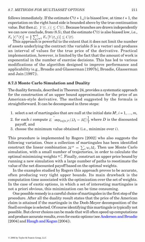
211
follows immediately. If the estimate Cl(t + 1, j) is biased low, at time t + 1, theexpectation on the right hand side is bounded above by the true continuationvalue. But then . Because branches are drawn independentlywe can now conclude, from (8.5), that the estimate Cl(t) is also biased low, i.e.,
This approach is powerful to the extent that it does not limit the numberof assets underlying the contract (the variable S is a vector) and producesan interval of values for the true price of the derivative. Practicalimplementation, however, is limited by the fact that the amount of work isexponential in the number of exercise decisions. This has led to variousmodifications of the algorithm designed to improve performance andapplicability (e.g., Broadie and Glasserman [1997b], Broadie, Glassermanand Jain [1997]).
8.7.3 Monte Carlo Simulation and Duality
The duality formula, described in Theorem 24, provides a systematic approachfor the construction of an upper bound approximation for the price of anAmerican-style derivative. The method suggested by the formula isstraightforward. It can be decomposed in three steps:
1. select a set of martingales that are null at the initial date Mi, i = 1, …, m,
2. for each i compute , where D is the discountedpayoff, and
3. choose the minimum value obtained (i.e., minimize over i).
This procedure is implemented by Rogers [2002] who also suggests thefollowing variation. Once a collection of martingales has been identifiedconstruct the linear combination . Then use Monte Carlosimulation, with a small number of trajectories, in order to calculate theoptimal minimizing weights . Finally, construct an upper price bound byrunning a new simulation with a large number of paths to reestimate thevalue of the net discounted payoff based on the optimal weights.
In the examples studied by Rogers this approach proves to be accurate,often producing very tight upper bounds. Its main drawback is thecomputation time associated with the optimization over the set of weights.In the case of exotic options, in which a set of interesting martingales isnot a priori obvious, this minimization can be time consuming.
One possible remedy is a careful choice of martingales in the first step of theprocedure. After all the duality result states that the price of the Americanclaim is attained if the martingale in the Doob-Meyer decomposition of theSnell envelope is selected. Of course identifying this martingale is typically notpossible. But clever choices can be made that will often speed up computations
8.7. METHODS FOR MULTIASSET OPTIONS
© 2006 by Taylor & Francis Group, LLC
and produce accurate results, even for exotic options (see Andersen and Broadie[2004] and Haugh and Kogan [2004]).

212 CHAPTER 8. NUMERICAL METHODS
8.8 Methods for Occupation Time DerivativesTo conclude this chapter we provide a survey of numerical methods foroccupation time derivatives. The path-dependent nature of these contractscomplicates their evaluation. Standard approaches nevertheless apply,modulo suitable modifications. The methods investigated include thosebased on the numerical inversion of Laplace transforms, PDE-basedmethods and Binomial/Trinomial trees.
8.8.1 Laplace Transforms
Valuation formulas for occupation time derivatives are often expressed interms of inverse Laplace transforms of density functions. In specific cases,such as the cumulative barrier claims (see section 7.6), the inverse Laplacetransform admits an explicit solution. The calculation of prices is thenreduced to the evaluation of the single or multiple integrals associatedwith the pricing operator and the claim’s payoff. Quadrature methods canbe used to carry out these integral evaluations.
In other cases, such as the Parisian option (see section 7.5), the inverseof the Laplace transform does not have an obvious analytical solution. Inthese situations the density function has an integral representation,resulting in additional integrals in the pricing formula. Quadraturemethods can again be used to handle the computation of these multipleintegrals. Numerical schemes based on approximations of inverse Laplacetransforms can also be employed. Approximation-based approaches thathave been used in the context of OTD pricing include the Weeks, Padé andFourier-series methods.
Calculation of prices based on Laplace transforms and their inversesare carried out by Chesney, Cornwall, Jeanblanc-Picqué, Kentwell andYor [1997], Hugonnier [1999], Linetsky [1999] and Fusai and Tagliani[2001]. Numerical schemes for inverting Laplace transforms can be foundin Singhal, Vlach and Vlach [1975], Davies and Martin [1979], Abate andWhitt [1992], Chaudhury, Lucantoni and Whitt [1994] and Craddock, Heathand Platen [2000].
8.8.2 PDE-based Methods
Consider a European-style occupation time derivative written on an assetprice S and depending on the time O spent by S in a constant set A. Let
be an open set with boundary . The derivative’s payoff is F(S, O, T) at the maturity date T in the event and G(S, D, t) if
and t ∈ [0, T]. Under standard differentiability assumptions thederivative’s price V (S, O, t) satisfies the fundamental valuation PDE
(8.6)
© 2006 by Taylor & Francis Group, LLC
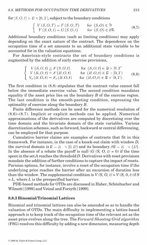
213
for , subject to the boundary conditions
(8.7)
Additional boundary conditions (such as limiting conditions) may applydepending on the exact nature of the contract. The dependence on theoccupation time of a set amounts to an additional state variable to beaccounted for in the valuation equations.
For American-style contracts the set of boundary conditions isaugmented by the addition of early exercise provisions,
(8.8)
The first condition in (8.8) stipulates that the contract value cannot fallbelow the immediate exercise value. The second condition mandatesequality if the asset price lies on the boundary B of the exercise region.The last condition is the smooth-pasting condition, expressing theoptimality of exercise along the boundary B.
Finite difference methods can be used for the numerical resolution of(8.6)–(8.7). Implicit or explicit methods can be applied. Numericalapproximations of the derivatives are computed by discretizing over thetime domain and the bivariate domain of the state variables. Variousdiscretization schemes, such as forward, backward or central differencing,can be employed for that purpose.
Cumulative barrier claims are examples of contracts that fit in thisframework. For instance, in the case of a knock-out claim with window D,the survival domain is and its boundary In the absence of a rebate the payoff is null (G (S, O, t) = 0) if the timespent in the set A reaches the threshold D. Derivatives with reset provisionsmandate the addition of further conditions to capture the impact of resets.Parisian options, for instance, involve a reset of the occupation time if theunderlying price reaches the barrier after an excursion of duration lessthan the window. The supplemental condition is V (S, O, t) = V (S, 0, t) if S= L, where L is the prespecified barrier.
PDE-based methods for OTDs are discussed in Haber, Schönbucher andWilmott [1999] and Vetzal and Forsyth [1999].
8.8.3 Binomial/Trinomial Lattices
Binomial and trinomial lattices can also be amended so as to handle thevaluation of OTDs. The main difficulty in implementing a lattice-basedapproach is to keep track of the occupation time of the relevant set as theasset price evolves along the tree. The Forward Shooting Grid algorithm(FSG) resolves this difficulty by adding a new dimension, measuring depth
8.8. METHODS FOR OCCUPATION TIME DERIVATIVES
© 2006 by Taylor & Francis Group, LLC

214 CHAPTER 8. NUMERICAL METHODS
(or height), to the tree. In effect the two-dimensional lattice becomes a three-dimensional lattice where the third dimension captures the number k ofoccurrences of the event (the number of time intervals spent in the set A).The lattice can be visualized as a superposition of planes, each correspondingto a value of the occupation counter. The top plane corresponds to a countequal to k = 0. The next one, one step below, to k = 1, and so on. When theasset price moves to a follower node, it remains in the same plane as longas the counter stays the same. If the counter increases by one unit, thefollower node is reached by taking a step down, i.e., moving down to thenext plane. Construction of the lattice proceeds in this manner untilmaturity.
Valuation is then carried out along familiar lines. The value at a givennode is obtained by taking the sum of the discounted values at followernodes. Follower nodes lie in the same plane if the counter stays the sameas the price moves to the follower node; they lie one step below if the counterincreases by a unit. The algorithm proceeds recursively, starting withterminal values, at the maturity date, and moving backward in time towardthe initial date. For a binomial lattice, with up and down steps (u, d), thisrecursion can be summarized by
(8.9)
for j = 1, …, n and k = 0, …, d. This backward recursion is subject to therelevant boundary conditions at the maturity date n and the upper boundof the occupation time domain d. American-style provisions can be readilyincorporated by taking the maximum of the continuation value, given bythe algorithm above, and the immediate exercise value. Claims with discretemonitoring dates can also be incorporated by selecting a time grid suchthat monitoring dates correspond to a multiple of the time step. Finally,claims with reset provisions can be handled by substituting the functiondescribing the dynamics of the counter k in the second argument of thecontinuation value, on the right hand side of (8.9). For a Parisian knock-out claim with window count d, based on the occupation time of the set A,this function is given by where x = Su or Sd.
The adaptation of the Forward Shooting Grid algorithm to OTDs is discussedby Kwok and Lau [2001] .6 FSG algorithms were originally pioneered by Hulland White [1993] and Ritchken, Sankarasubramaniam and Vijh [1993] inorder to price Asian and Lookback options. Further results about the methodcan be found Barraquand and Pudet [1996].
6Another lattice-based approach is proposed by Avellaneda and Wu [1999]. Their methoduses the density function of the relevant hitting time in order to identify the appropriateboundary conditions in the tree.
© 2006 by Taylor & Francis Group, LLC
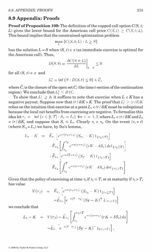
215
8.9 Appendix: ProofsProof of Proposition 109: The definition of the capped call option C(S, t;L) gives the lower bound for the American call price This bound implies that the constrained optimization problem
has the solution L = S when (S, t) ∈ ε (as immediate exercise is optimal forthe American call). Thus,
for all (S, t) ∈ ε and
where C–
t is the closure of the open set Ct (the time t-section of the continuationregion). We conclude that .
To show that it suffices to note that exercise when L < K has anegative payout. Suppose now that (r/δ)K > K. The proof that relies on the intuition that exercise at a point L1 < (r/δ)K must be suboptimalbecause the local net benefits from exercising are negative. To formalize thisidea let where L1 < (r/δ)K and L2
= (r/δ)K, and suppose that St � L1. Clearly �1 < �2. On the event {�1 = t}(where S�1 = L1) we have, by Ito’s lemma,
Given that the policy of exercising at time �2 if �2 � T, or at maturity if �2 > T,has value
we conclude that
8.9. APPENDIX: PROOFS
© 2006 by Taylor & Francis Group, LLC

216 CHAPTER 8. NUMERICAL METHODS
which implies (since rK - δSv > 0 for t � �2). We concludethat immediate exercise at is dominated by the policy ofwaiting until L2 is reached.
For the limiting values of L* note that when t → T the optimal exerciseboundary for the call option converges to the point, Giventhat for t ∈ [0, T) we obtain When T– t → ∞ the American call has a constant exercise boundary equal to
(see Corollary 35). This policy lies in the class ofconstant barrier policies. It follows immediately that converges to B-∞. �
Proof of Proposition 110: The proof is outlined in the text following theproposition. �
© 2006 by Taylor & Francis Group, LLC

Bibliography
[1] Abate, J. and W.Whitt, “The Fourier-Series Method for InvertingTransforms of Probability Distributions,” Queueing Systems, 10, 1992,5–88.
[2] Ait-Sahlia, F., “Optimal Stopping and Weak Convergence Methods forSome Problems in Financial Economics,” Ph.D. Dissertation, StanfordUniversity, 1995.
[3] Akahori, J., “Some Formulae for a New Type of Path-Dependent Option,”Annals of Applied Probability, 5, 1995, 383–388.
[4] Amin, K., “On the Computation of Continuous Time Option Prices usingDiscrete Approximations,” Journal of Financial and Quantitative Analysis,26, 1991, 477–496.
[5] Amin, K. and A.Khanna, “Convergence of American Option Values fromDiscrete- to Continuous-Time Financial Models,” Mathematical Finance,4, 1994, 289–304.
[6] Andersen, L. and M.Broadie, “A Primal-Dual Simulation Algorithm forPricing Multi-Dimensional American Options,” Management Science, 50,2004, 1222–1234.
[7] Avellaneda, M. and L.Wu, “Pricing Parisian-Style Options with a LatticeMethod,” International Journal of Theoretical and Applied Finance, 2, 1999,1–16.
[8] Bachelier, L., “Théorie de la Spéculation,” Annales de l’École NormaleSupérieure, 17, 1900, 21–86. In The Random Character of Stock MarketPrices, Paul H.Cottner ed., The MIT Press, Cambridge, Mass., 1964.
[9] Barles, G., J.Burdeau, M.Romano and N.Samsoen, “Critical Stock PriceNear Expiration,” Mathematical Finance, 5, 1995, 77–95.
© 2006 by Taylor & Francis Group, LLC

BIBLIOGRAPHY218
[10] Barone-Adesi, G. and R.Whaley, “Efficient Analytical Approximation ofAmerican Option Values,” Journal of Finance, 42, 1987, 301–320.
[11] Barraquand, J. and D.Martineau, “Numerical Valuation of HighDimensional Multivariate American Securities,” Journal of Financial andQuantitative Analysis, 30, 1995, 383–405.
[12] Barraquand, J. and T.Pudet, “Pricing of American Path DependentContingent Claims,” Mathematical Finance, 6, 1996, 17–51.
[13] Bensoussan, A., “On the Theory of Option Pricing,” Acta ApplicandaeMathematicae, 2, 1984, 139–158.
[14] Bergman, Y., B.Grundy and Z.Wiener, “General Properties of Option Prices,”Journal of Finance, 51, 1996, 1573–1610.
[15] Bermin, H.P., “A General Approach to Hedging Options: Applications toBarrier and Partial Barrier Options,” Mathematical Finance, 12, 2002,199–218.
[16] Bermin, H.P., “Hedging Options: The Malliavin Calculus Approach versusthe Delta-Hedging Approach,” Mathematical Finance, 13, 2003, 73–84.
[17] Bjerksund, P. and G.Stensland, “Closed Form Approximation of AmericanOptions,” Scandinavian Journal of Management, 1992.
[18] Bjerksund, P. and G.Stensland, “American Exchange Options and a Put-Call Transformation: A Note,” Journal of Business, Finance and Accounting,20, 1993, 761–764.
[19] Black, F. and J.Cox, “Valuing Corporate Securities: Some Effects of BondIndenture Provisions,” Journal of Finance, 31, 1976, 351–367.
[20] Black, F. and M.Scholes, “The Pricing of Options and Corporate Liabilities,”Journal of Political Economy, 81, 1973, 637–654.
[21] Boyle, P.P., “Options: A Monte Carlo Approach,” Journal of FinancialEconomics, 4, 1977, 323–338.
[22] Boyle, P.P., “A Lattice Framework for Option Pricing with Two StateVariables,” Journal of Financial and Quantitative Analysis, 23, 1988,1–12.
[23] Boyle, P.P., “Barrier Options,” Working paper, University of Waterloo,1992.
[24] Boyle, P.P., M.Broadie and P.Glasserman, “Monte Carlo Methods forSecurity Pricing,” Journal of Economic Dynamics and Control, 21, 1997,1276–1321.
© 2006 by Taylor & Francis Group, LLC

219BIBLIOGRAPHY
[25] Boyle, P.P., J.Evnine and S.Gibbs, “Numerical Evaluation of MultivariateContingent Claims,” Review of Financial Studies, 2, 1989, 241–250.
[26] Boyle, P.P. and S.M.Turnbull, “Pricing and Hedging Capped Options,”Journal of Futures Markets, 9, 1989, 41–54.
[27] Breen, R., “The Accelerated Binomial Option Pricing Model,” Journal ofFinancial and Quantitative Analysis, 26, 1991, 153–164.
[28] Brennan, M. and E.Schwartz, “The Valuation of American Put Options,”Journal of Finance, 32, 1977, 449–462.
[29] Brennan, M. and E.Schwartz, “Finite Difference Methods and JumpProcesses Arising in the Pricing of Contingent Claims: A Synthesis,”Journal of Financial and Quantitative Analysis, 13, 1978, 461–474.
[30] Broadie, M. and J.B.Detemple, “American Capped Call Options onDividend-Paying Assets,” Review of Financial Studies, 8, 1995, 161–191.
[31] Broadie, M. and J.B.Detemple, “American Option Valuation: New Bounds,Approximations, and a Comparison of Exisiting Methods,” Review ofFinancial Studies, 9, 1996, 1211–1250.
[32] Broadie, M. and J.B.Detemple, “The Valuation of American Options onMultiple Assets,” Mathematical Finance, 7, 1997a, 241–285.
[33] Broadie, M. and J.B.Detemple, “Recent Advances in Numerical Methodsfor Pricing Derivative Securities,” Numerical Methods in Finance, L.C.G.Rogers and D.Talay, eds., Cambridge University Press, Cambridge,1997b, 43–66.
[34] Broadie, M. and J.B.Detemple, “American Options on Dividend PayingAssets,” in Topology and Markets, G.Chichilnisky, ed., Fields InstituteCommunications, 22, 1999, 69–97.
[35] Broadie, M. and J.B.Detemple, “Option Pricing: Valuation Models andApplications,” Management Science, 50, 2004, 1145–1177.
[36] Broadie, M. and P.Glasserman, “Pricing American-Style Securities UsingSimulation,” Journal of Economic Dynamics and Control, 21, 1997a, 1323–1352.
[37] Broadie, M. and P.Glasserman, “A Stochastic Mesh Method for PricingHigh-Dimensional American Options,” Working Paper, ColumbiaUniversity, 1997b.
[38] Broadie, M., P.Glasserman and G.Jain, “Enhanced Monte Carlo Estimatesfor American Option Prices,” Journal of Derivatives, 5, 1997, 25–44.
© 2006 by Taylor & Francis Group, LLC

BIBLIOGRAPHY220
[39] Bunch, D.S. and H.Johnson, “A Simple and Numerically EfficientValuation Method for American Puts Using a Modified Geske-JohnsonApproach,” Journal of Finance, 47, 1992, 809–816.
[40] Carr, P., “Randomization and the American Put,” Review of FinancialStudies, 11, 1998, 597–626.
[41] Carr, P. and D.Faguet, “Fast Accurate Valuation of American Options,”Working paper, Cornell University, 1995.
[42] Carr, P., R.Jarrow and R.Myneni, “Alternative Characterizations ofAmerican Put Options,” Mathematical Finance, 2, 1992, 87–106.
[43] Carr, P. and R.Jarrow, “The Stop-Loss Start-Gain Paradox and OptionValuation: A New Decomposition into Intrinsic and Time Value,” Reviewof Financial Studies, 3, 1990, 469–492.
[44] Carriere, J., “Valuation of the Early-Exercise Price for Options UsingSimulations and Nonparametric Regression,” Insurance, Mathematics andEconomics, 19, 1996, 19–30.
[45] Chaudhury, G.L., Lucantoni, D.M. and W.Whitt, “MultidimensionalTransform Inversion with Applications to the Transient M/G/1 Queue,”Annals of Applied Probability, 5, 1994, 389–398.
[46] Chesney, M., J.Cornwall, M.Jeanblanc-Picqué, G.Kentwell and M.Yor,“Parisian Pricing,” Risk, 10, 1997, 77–79.
[47] Chesney, M., M.Jeanblanc-Picqué and M.Yor, “Brownian Excursions andParisian Barrier Options,” Advances in Applied Probability, 29, 1997,165–184.
[48] Cheyette, O., “Pricing Options on Multiple Assets,” Advances in Futuresand Options Research, 4, 1990, 69–81.
[49] Cottle, R., J.-S.Pang and R.Stone, The Linear Complementarity Problem,Academic Press, Boston, 1992.
[50] Courtadon, G., “A More Accurate Finite Difference Approximation for theValuation of Options,” Journal of Financial and Quantitative Analysis, 17,1982, 697–705.
[51] Cox, J.C., “Notes on Options I: Constant Elasticity of Variance Diffusion,”working paper, Stanford University, 1975.
[52] Cox, J.C., “The Constant Elasticity of Variance Option Pricing Model,”Journal of Portfolio Management, 22, 1996, 15–17.
[53] Cox, J. and S.Ross, “The Valuation of Options for Alternative StochasticProcesses,” Journal of Financial Economics, 3, 1976, 145–166.
© 2006 by Taylor & Francis Group, LLC

221BIBLIOGRAPHY
[54] Cox, J.C., S.A.Ross and M.Rubinstein, “Option Pricing: A SimplifiedApproach,” Journal of Financial Economics, 7, 1979, 229–263.
[55] Cox, J. and M.Rubinstein, Option Markets, Prentice Hall, Englewood Cliffs,New Jersey, 1985.
[56] Craddock, M., D.Heath and E.Platen, “Numerical Inversion of LaplaceTransforms: A Survey of Techniques with Applications to DerivativePricing,” Journal of Computational Finance, 4, 2000, 57–81.
[57] Curran, M., “Accelerating American Option Pricing in Lattices,” Journalof Derivatives, 3, 1995, 8–17.
[58] Dassios, A., “The Distribution of the Quantile of a Brownian Motion withDrift and the Pricing of Related Path-Dependent Options,” Annals of AppliedProbability, 5, 1995, 389–398.
[59] Davies, B. and B.Martin, “Numerical Inversion of the Laplace Transform:A Survey and Comparison of Methods,” Journal of Computational Physics,33, 1979, 1–32.
[60] Davis, M.H.A. and I.Karatzas, “A Deterministic Approach to OptimalStopping, with Applications,” in Probability, Statistics and Optimization:A Tribute to Peter Whittle, F.P.Kelly, ed., Wiley, New York, 1994, 455–466.
[61] Davydov, D. and V.Linetsky, “The Valuation and Hedging of Barrier andLookback Options under the CEV Process,” Management Science, 47, 2001,949–965.
[62] Detemple, J.B., “American Options: Symmetry Properties,” Handbooks inMathematical Finance: Topics in Option Pricing, Interest Rates and RiskManagement, J.Cvitanic, E.Jouini and M.Musiela, eds., CambridgeUniversity Press, Cambridge, England, 2001, 67–104.
[63] Detemple, J.B., S.Feng and W.Tian, “The Valuation of American CallOptions on the Minimum of Two Dividend-paying Assets,” Annals ofApplied Probability, 13, 2003, 953–983.
[64] Detemple, J.B., R.Garcia and M.Rindisbacher, “A Monte-Carlo Methodfor Optimal Portfolios,” Journal of Finance, 58, 2003, 401–446.
[65] Detemple, J.B. and W.Tian, “The Valuation of American Options for aClass of Diffusion Processes,” Management Science, 48, 2002, 917–937.
[66] Diener, F. and M.Diener, “Asymptotics of the Price Oscillations of a VanillaOption in a Tree Model,” Mathematical Finance, 13, 2004, 271–294.
[67] Dixit, A. and R.Pindyck, Investment Under Uncertainty, Princeton UniversityPress, 1994.
© 2006 by Taylor & Francis Group, LLC

BIBLIOGRAPHY222
[68] Duffie, D., “Stochastic Equilibria: Existence, Spanning Number, and The‘No Expected Financial Gain From Trade’ Hypothesis,” Econometrica, 54,1986, 1161–1184.
[69] El Karoui, N., M.Jeanblanc-Picque and S.Shreve, “Robustness of the Blackand Scholes Formula,” Mathematical Finance, 8, 1998 93–126.
[70] El Karoui, N. and I.Karatzas, “A New Approach to the Skorohod Problemand its Applications,” Stochastics and Stochastics Reports, 34, 1991,57–82.
[71] El Karoui, N., Les Aspects Probabilistes du Controle Stochastique, LectureNotes in Mathematics, 876, Springer-Verlag, Berlin, 1981, 73–238.
[72] Emanuel, D.C. and J.D.MacBeth, “Further Results on the ConstantElasticity of Variance Call Option Pricing Model,” Journal of Financialand Quantitative Analysis, 7, 1984, 533–54.
[73] Embrecht, P., L.C.G.Rogers and M.Yor, “A Proof of Dassios’ Representationof the α-Quantile of Brownian Motion with Drift,” Annals of AppliedProbability, 5, 1995, 757–767.
[74] Evans, J.D., R.Kuske and J.B.Keller, “American Options on Assets withDividends near Expiry,” Mathematical Finance, 12, 2002, 219–237.
[75] Flesaker, B., “The Design and Valuation of Capped Stock Index Options,”Working Paper, University of Illinois at Urbana-Champaign, 1992.
[76] Fournié, E., J.-M.Lasry, J.Lebuchoux, P.-L Lions and N.Touzi, “Applicationsof Malliavin Calculus to Monte Carlo Methods in Finance,” Finance andStochastics, 3, 1999, 391–412.
[77] Francois, P. and E.Morellec, “Capital Structure and Asset Prices: SomeEffects of Bankruptcy Procedures,” Journal of Business, 77, 2004,387–411.
[78] Fusai, G., “Corridor Options and Arc-Sine Law,” Annals of AppliedProbability, 10, 2000, 634–663.
[79] Fusai, G. and A.Tagliani, “Pricing of Occupation Time Derivatives:Continuous and Discrete Monitoring,” Journal of Computational Finance,5, 2001, 1–37.
[80] Galai, D., A.Raviv and Z.Wiener, “Liquidation Triggers and the Valuationof Equity and Debt,” Working paper, Hebrew University of Jerusalem,2005.
[81] Gao, B., J.-z.Huang and M.Subrahmanyam, “The Valuation of AmericanBarrier Options Using the Decomposition Technique,” Journal of EconomicDynamics and Control, 24, 2000, 1783–1827.
© 2006 by Taylor & Francis Group, LLC

223BIBLIOGRAPHY
[82] Geltner, D., T.Riddiough and S.Stojanovic, “Insights on the Effect of LandUse Choice: The Perpetual Option on the Best of Two Underlying Assets,”Journal of Urban Economics, 39, 1996, 20–50.
[83] Geman H., N.El Karoui and J.-C.Rochet, “Changes of Numeraire, Changesof Probability Measure and Option Pricing,” Journal of Applied Probability,32, 1995, 443–458.
[84] Geske, R., “A Note on an Analytical Valuation Formula for UnprotectedAmerican Options on Stocks with Known Dividends,” Journal of FinancialEconomics, 7, 1979, 375–380.
[85] Geske, R. and H.Johnson, “The American Put Option Valued Analytically,”Journal of Finance, 39, 1984, 1511–1524.
[86] Grabbe, O., “The Pricing of Call and Put Options on Foreign Exchange,”Journal of International Money and Finance, 2, 1983, 239–253.
[87] Haber, R.J., P.J.Schönbucher and P.Wilmott, “Pricing Parisian Options,”Journal of Derivatives, 6, 1999, 71–79.
[88] Harrison, M. and D.Kreps, “Martingales and Arbitrage in MultiperiodSecurity Markets,” Journal of Economic Theory, 20, 1979, 381–408.
[89] Harrison, M. and S.Pliska, “Martingales and Stochastic Integrals in theTheory of Continuous Trading,” Stochastic Processes and Their Applications,”11, 1981, 215–260.
[90] Haugh, M. and L.Kogan, “Approximating Pricing and Exercising of High-Dimensional American Options: A Duality Approach,” Operations Research,52, 2004, 258–270.
[91] He, H., “Convergence from Discrete- to Continuous-Time Contingent ClaimPrices,” Review of Financial Studies, 3, 1990, 523–546.
[92] Ho, T.S., S.Stapleton and M.G.Subrahmanyam, “A Simple Technique forthe Valuation and Hedging of American Options,” Journal of Derivatives,2, 1994, 52–66.
[93] Hobson, D.G., “Robust Hedging via Coupling,” Finance and Stochastics, 2,1998, 329–347.
[94] Huang, J., M.Subrahmanyam and G.Yu, “Pricing and Hedging AmericanOptions: A Recursive Integration Method,” Review of Financial Studies, 9,1996, 277–330.
[95] Hugonnier, J., “The Feynman-Kac Formula and Pricing Occupation TimesDerivatives,” International Journal of Theoretical and Applied Finance, 2,1999, 153–178.
© 2006 by Taylor & Francis Group, LLC

BIBLIOGRAPHY224
[96] Hull, J., Options, Futures and Other Derivatives, 5th edition, Prentice Hall,New Jersey, 2002.
[97] Hull, J. and A.White, “The Use of Control Variate Techniques in OptionPricing,” Journal of Financial and Quantitative Analysis, 23, 1988,237–251.
[98] Hull, J. and A.White, “Valuing Derivative Securities Using the ExplicitFinite Difference Method,” Journal of Financial and Quantitative Analysis,25, 1990, 87–100.
[99] Hull, J. and A.White, “Efficient Procedures for Valuing European andAmerican Path-Dependent Options,” Journal of Derivatives, 1, 1993, 21–32.
[100] Jacka, S.D., “Optimal Stopping and the American Put,” MathematicalFinance, 1, 1991, 1–14.
[101] Jacka, S.D. and J.Lynn, “Finite-Horizon Optimal Stopping, ObstacleProblems and the Shape of the Continuation Region,” Stochastics andStochastics Reports, 39, 1992, 25–42.
[102] Jaillet, P., D.Lamberton and B.Lapeyre, “Variational Inequalities andthe Pricing of American Options,” Acta Applicandae Mathematicae, 21,1990, 263–289.
[103] Jarrow, R. and A.Rudd, Option Pricing, Dow Jones—Irwin, Homewood,Illinois, 1983.
[104] Johnson, H., “The Pricing of Complex Options,” Working paper, LouisianaState University, 1981.
[105] Johnson, H., “An Analytic Approximation for the American Put Price,”Journal of Financial and Quantitative Analysis, 18, 1983, 141–148.
[106] Johnson, H., “Options on the Maximum or the Minimum of Several Assets,”Journal of Financial and Quantitative Analysis, 22, 1987, 227–283.
[107] Ju, N., “Pricing an American Option by Approximating Its Early ExerciseBoundary as a Multi-Piece Exponential Function,” Review of FinancialStudies, 11, 1998, 627–646.
[108] Kac, M., “On Distributions of Certain Wiener Functionals,” Transactionsof the American Mathematical Society, 65, 1949, 1–13.
[109] Kac, M., “On Some Connections Between Probability and Differential andIntegral Equations,” Proceedings of the 2nd Berkeley Symposium onMathematical Statistics and Probability, 1951, 189–215.
© 2006 by Taylor & Francis Group, LLC

225BIBLIOGRAPHY
[110] Kallast, S. and A.Kivinukk, “Pricing and Hedging American Options UsingApproximations by Kim Integral Equations,” European Finance Review, 7,2003, 361–383.
[111] Kamrad, B. and P.Ritchken, “Multinomial Approximating Models forOptions with k State Variables,” Management Science, 37, 1991,1640–1652.
[112] Karatzas, L., “On the Pricing of American Options,” Appl. Math. Optim.,17, 1988, 37–60.
[113] Karatzas, I. and S.Shreve, Brownian Motion and Stochastic Calculus,Springer-Verlag, New York, 1988.
[114] Karatzas, I. and S.Shreve, Methods of Mathematical Finance, Springer-Verlag, New York, 1998.
[115] Kholodnyi, V.A. and J.F.Price, Foreign Exchange Option Symmetry, WorldScientific, London, 1998.
[116] Kim, I.J., “The Analytic Valuation of American Options,” Review of FinancialStudies, 3, 1990, 547–572.
[117] Kim, I.J. and S.Byun, “Optimal Exercise Boundary in a Binomial OptionPricing Model,” Journal of Financial Engineering, 3, 1994, 137–158.
[118] Kim, I.J. and G.Yu, “An Alternative Approach to the Valuation of AmericanOptions and Applications,” Review of Derivatives Research, 1, 1996, 61–86.
[119] Kwok, Y.K. and K.W.Lau, “Pricing Algorithms for Options with ExoticPath-Dependence,” Journal of Derivatives, Fall 2001, 28–38.
[120] Lamberton, D., “Convergence of the Critical Price in the Approximation ofAmerican Options,” Mathematical Finance, 3, 1993, 179–190.
[121] Lamberton, D., “Error Estimates for the Binomial Approximation ofAmerican Put Options,” Annals of Applied Probability, 8, 1998, 206–233.
[122] Lamberton, D., “Brownian Optimal Stopping and Random Walks,” AppliedMathematics and Optimization, 45, 2002, 283–324.
[123] Leisen, D. and M.Reimer, “Binomial Models for Option Valuation—Examining and Improving Convergence,” Working paper B-309, Universityof Bonn, Bonn, 1995.
[124] Lintner, J., “The Valuation of Risky Assets and the Selection of RiskyInvestments in Stock Portfolios and Capital Budgets,” Review of Economicsand Statistics, 47, 1965, 13–37.
© 2006 by Taylor & Francis Group, LLC

BIBLIOGRAPHY226
[125] Little, T., V.Pant and C.Hou, “A New Integral Representation of the EarlyExercise Boundary for American Put Options,” Journal of ComputationalFinance, 2000.
[126] Longstaff, F.A. and E.A.Schwartz, “Valuing American Options bySimulations: A Simple Least-Squares Approach,” Review of FinancialStudies, 14, 2001, 113–147.
[127] Madan, D., F.Milne and H.Shefrin, “The Multinomial Option Pricing Modeland its Brownian and Poisson Limits,” Review of Financial Studies, 4,1989, 251–266.
[128] Marchuk, G. and V.Shaidurov, Difference Methods and Their Extrapolations,Springer-Verlag, New York, 1983.
[129] Margrabe, W., “The Value of an Option to Exchange One Asset for Another,”Journal of Finance, 33, 1978, 177–186.
[130] McDonald, R. and M.Schroder, “A Parity Result for American Options,”Journal of Computational Finance, 1998. Working paper, NorthwesternUniversity, 1990.
[131] McKean, H.P., “A Free Boundary Problem for the Heat Equation Arisingfrom a Problem in Mathematical Economics,” Industrial ManagementReview, 6, 1965, 32–39.
[132] Merton, R.C., “Theory of Rational Option Pricing,” Bell Journal of Economicsand Management Science, 4, 1973a, 141–183.
[133] Merton, R.C., “An Intertemporal Capital Asset Pricing Model,”Econometrica, 41, 1973b, 867–888.
[134] Moraux, F., “On Cumulative Parisian Options,” Finance, 23, 202,127–132.
[135] Moraux, F., “Valuing Corporate Liabilities When the Default ThresholdIs not an Absorbing Barrier,” Working paper, Universite de Rennes 1,2004.
[136] Mossin, J., “Security Pricing and Investment Criteria in CompetitiveMarkets,” American Economic Review, 59, 1969, 749–756.
[137] Miura, R, “A Note on Look-Back Options based on Order Statistics,”Hitosubashi Journal of Commerce and Management, 27, 1992, 15–28.
[138] Myneni, R., “The Pricing of the American Option,” Annals of AppliedProbability, 2, 1992, 1–23.
[139] Ocone, D. and I.Karatzas, “A Generalized Clark Representation Formula,with Application to Optimal Portfolios,” Stochastics 34, 187–220.
© 2006 by Taylor & Francis Group, LLC

227BIBLIOGRAPHY
[140] Omberg, E., “The Valuation of American Put Options with ExponentialExercise Policies,” Advances in Futures and Options Research, 2, 1987, 117–142.
[141] Omberg, E., “Efficient Discrete Time Jump Process Models in OptionPricing,” Journal of Financial and Quantitative Analysis, 23, 1988,161–174.
[142] Parkinson, M., “Option Pricing: The American Put,” Journal of Business,50, 1977, 21–36.
[143] Press, W., S.Teukolsky, W.Vetterling and B.Flannery, Numerical Recipesin C: The Art of Scientific Computing, 2nd edition, Cambridge UniversityPress, Cambridge, England, 1992.
[144] Raymar, S. and M.Zwecher, “A Monte Carlo Valuation of American CallOptions on the Maximum of Several Stocks,” Journal of Derivatives, 5,1997, 7–23.
[145] Rendleman, R. and B.Bartter, “Two-State Option Pricing,” Journal ofFinance, 34, 1979, 1093–1110.
[146] Ritchken, P., L.Sankarasubramaniam and A.M.Vijh, “The Valuation ofPath Dependent Contracts on the Average,” Management Science, 39, 1993,1202–1213.
[147] Rogers, C., “Monte Carlo Valuation of American Options,” MathematicalFinance, 12, 2002, 271–286.
[148] Roll, R., “An Analytic Valuation Formula for Unprotected American CallOptions on Stocks with Known Dividends,” Journal of Financial Economics,5, 1977, 251–258.
[149] Rubinstein, M., “One for Another,” Risk, 4, 1991, 30–32.
[150] Rubinstein, M., “Return to Oz,” Risk, 7, 1994, 67–71.
[151] Rubinstein M. and E.Reiner, “Breaking Down the Barriers,” Risk, 4, 1991,28–35.
[152] Rutkowski, M., “The Early Exercise Premium Representation of ForeignMarket American Options,” Mathematical Finance, 4, 1994, 313–325.
[153] Samuelson, P.A., “Rational Theory of Warrant Pricing,” IndustrialManagement Review, 6, 1965, 13–31.
[154] Schroder, M., “Computing the Constant Elasticity of Variance OptionPricing Formula,” Journal of Finance, 44, 1989, 211–219.
[155] Schroder, M., “Changes of Numeraire for Pricing Futures, Forwards andOptions,” Review of Financial Studies, 12, 1999, 1143–1163.
© 2006 by Taylor & Francis Group, LLC

BIBLIOGRAPHY228
[156] Schwartz, E.S., “The Valuation of Warrants: Implementing a NewApproach,” Journal of Financial Economics, 4, 1977, 79–93.
[157] Sharpe, W., “Capital Asset Prices: A Theory of Market Equilibrium underConditions of Risk,” Journal of Finance, 19, 1964, 425–442.
[158] Singhal, K., J.Vlach and M.Vlach, “Numerical Inversion ofMultidimensional Laplace Transforms,” Proceedings of the IEEE, 63, 1975,1627–1628.
[159] Stulz, R.M., “Options on the Minimum or the Maximum of Two RiskyAssets,” Journal of Financial Economics, 10, 1982, 161–185.
[160] Takács, L., “On a Generalization of the Arc-Sine Law,” Annals of AppliedProbability, 6, 1996, 1035–1040.
[161] Tan, K. and K.Vetzal, “Early Exercise Regions for Exotic Options,” un-published manuscript, University of Waterloo, 1994.
[162] Tian, Y., “A Modified Lattice Approach to Option Pricing,” Journal ofFutures Markets, 13, 1993, 563–577.
[163] Tilley, J., “Valuing American Options in a Path Simulation Model,”Transactions of the Society of Actuaries, 45, 1993, 83–104.
[164] Trigeorgis, L., “A Log-transformed Binomial Numerical Analysis Methodfor Valuing Complex Multi-Option Investments,” Journal of Financialand Quantitative Analysis, 26, 1991, 309–326.
[165] Van Moerbeke, P., “On Optimal Stopping and Free Boundary Problems,”Arch. Rational Mech. Analysis, 60, 1976, 101–148.
[166] Vetzal, K.R. and P.A.Forsyth, “Discrete Parisian and Delayed BarrierOptions: A General Numerical Approach,” Advances in Futures and OptionsResearch, 10, 1999, 1–15.
[167] Wu, L., Y.K.Kwok and H.Yu, “Asian Options with the American EarlyExercise Feature,” International Journal of Theoretical and Applied Finance,2, 1999, 101–111.
[168] Yor, M., “The Distribution of Brownian Quantiles,” Journal of AppliedProbability, 32, 1995, 405–416.
© 2006 by Taylor & Francis Group, LLC