American Journal of Political Science

An Integrated Theory of Budgetary Politics and Some Empirical Tests: The USNational Budget, 1791-2010

--Manuscript Draft--

Manuscript Number: AJPS-36433R1

Full Title: An Integrated Theory of Budgetary Politics and Some Empirical Tests: The USNational Budget, 1791-2010

Article Type: Article

Keywords: expenditures, budgets, exponential growth, path dependency, incrementalism

Corresponding Author: Bryan JonesUniversity of Texas at AustinAustin, TX UNITED STATES

Corresponding Author SecondaryInformation:

Corresponding Author's Institution: University of Texas at Austin

Corresponding Author's SecondaryInstitution:

First Author: Bryan Jones

First Author Secondary Information:

Order of Authors: Bryan Jones

Laszlo Zalanyi, PhD

Peter Erdi, PhD

Order of Authors Secondary Information:

Abstract: We develop a more general theory budgetary politics and examine its implications on anew dataset on US government expenditures from 1791 to 2010. We draw on threemajor approaches to budgeting: the decision-making theories, primarilyincrementalism, and serial processing; the policy process models, basically extensionsof punctuated equilibrium; and path dependency. We show that the incrementalistbudget model is recursive, and its solution is exponential growth. We assess pathdependency by assessing the extent to which the growth curve has a constantexponent and intercept, except when critical junctures, associated with wars oreconomic collapse, occur. A second type of disruption occurs in the churning thatoccurs during the equilibrium periods, assessed by examining the non-Gaussiancharacter of the deviations from the growth curve for the equilibrium periods. Empiricaltests indicate support for the theory, but with inconsistent findings, particularlyadjustments that occur in the absence of critical junctures.

Response to Reviewers: We appreciate the opportunity to revise our paper for the American Journal of PoliticalScience. Below we highlight what we have done in response to the editor’s and thereviewers’ comments.

Threading through all the reviews, and strongly highlighted by the editor, was the needto make clear the purpose of the manuscript. Reviewer 1’s critique centers almostexclusively on these points, Reviewer 2 similarly notes that “My suggestions forimprovements of the paper regard first and foremost the motivation and structure of thepaper.” We read Reviewer 3 as not comfortable with using ‘go-to’ arguments withoutincorporating them into a broader historical narrative.

The earlier draft concentrated on moving our understanding of budgeting from an a-historical focus to one incorporating longer run dynamics, using some innovativemethods to do so. It relied more on empirical generalizations from strong newanalytical techniques and linking to well-established pieces of budgetary theory.

Powered by Editorial Manager® and Preprint Manager® from Aries Systems Corporation

What we missed in this exercise is how close we were to being able to formulate andtest a general theory of the politics of budgeting that extended existing understandingstemporally (Reviewer 2 indicates the weaknesses of current budgetary studies is thatthey do not “reveal anything about the more precise budget dynamics over time” (thereviewer is referring to a particular paper, but the critique is general). Our contributionin this draft in essence incorporates all three major approaches to the study ofbudgeting: decision-making approaches (in which individual budget actors are thefocus, with the major approach being incrementalism), policy process approaches (inwhich the system of actors are the focus, with punctuated equilibrium being the majortheoretical perspective), and historical institutionalism (with its focus on pathdependency and critical junctures, which has not seriously been used in budgetstudies, but clearly should be). This is what we have done in this version; in essence,we have “gone long”. This has the advantage of offering a top-down approach to whatwe have done, highlighting how closely the overall data series fits the theory of‘disrupted exponential incrementalism”, as we have termed it (suggestions for a betterterm welcome). It also allows for highlighting explicitly where the data do not fit theseries, and there are several places where it does not. This is particularly true for thePost WWII period, as we note in the conclusion.

This approach responds to the first two comments by the editor, which emphasize thatthe paper was unpersuasive in its motivation, referring to comments by both Reviewer1 and Reviewer 2. It also addresses the third comment by the editor, “I would like tosee more than making an empirical generalization”. And it addresses, we think,Reviewer 2’s observation that It would be helpful in further developing this researchagenda if expressions such as ‘the potential of churning within periods of steadyexponential growth’ ‘stable but nevertheless noisy periods’ and permanent ratchets’could be integrated into a more systematic conceptualization of budget changes”.

Specifics

We have addressed the editor’s third comment, based on observations by Reviewer 2)that some technical material could be put into an on-line appendix. That on-lineappendix also includes details on the construction of the dataset.

We have addressed the editor’s fourth comment, and Reviewer 2’s suggestion that weprovide an example of the differences in real dollars the shift from linear to exponentialmakes, as well as the change from an exponent of say .03 to .04 (a real shift from ouranalysis) on page 14. We have tried to address Reviewer 3’s request for a morehistorical type example on p.11.

We’ve added some brief explanatory text below the figures to link the technicaldiagrams directly to the development of the argument in the paper. This is becomingmore common in political science papers, and we think it works especially well in thispaper.

Reviewer 3 is most explicit in tying budget history to the budget trends we detect, andraises some important issues. All of his/her points are reasonable and intriguing, butin the end we ran out of room to address these matters in sufficient detail. However wehave discussed what we see as the most important historical puzzle: the failure ofnegative feedback processes to restore exponential equilibrium in some times forsome policies. In the last paragraph we note that the final period in particular does notfit the exponential equilibrium very well, and speculate a little about why.

Powered by Editorial Manager® and Preprint Manager® from Aries Systems Corporation

An Integrated Theory of Budgetary Politics and Some Empirical Tests: The US National Budget, 1791-2010

Manuscript ( Not to include ANY author-identifying information)

Abstract

We develop a more general theory budgetary politics and examine its implications

on a new dataset on US government expenditures from 1791 to 2010. We draw on three

major approaches to budgeting: the decision-making theories, primarily incrementalism,

and serial processing; the policy process models, basically extensions of punctuated

equilibrium; and path dependency. We show that the incrementalist budget model is

recursive, and its solution is exponential growth. We assess path dependency by assessing

the extent to which the growth curve has a constant exponent and intercept, except when

critical junctures, associated with wars or economic collapse, occur. A second type of

disruption occurs in the churning that occurs during the equilibrium periods, assessed by

examining the non-Gaussian character of the deviations from the growth curve for the

equilibrium periods. Empirical tests indicate support for the theory, but with inconsistent

findings, particularly adjustments that occur in the absence of critical junctures.

Manuscript word count: 8736.

1

An Integrated Theory of Budgetary Politics and Some Empirical Tests 1

Three-quarters of a century ago, V.O. Key (1940) commented that no budget theory

existed. Key was discussing a normative theory of budget allocation, but he recognized the

limits of any normative theory unsupported by empirical study. Today we have several

budgetary theories, and an increasing number of studies of budgetary allocations across

several countries. Yet it is fair to say that we continue to lack a comprehensive empirically-

based budgetary theory. If we are to achieve that more comprehensive theory, we will

need to be able both to unify the strong theories we have at present, and to extend them

through much longer time periods than scholars have been able to do to date. In this paper,

we develop a more general theory of budgetary allocations, termed disrupted exponential

incrementalism. Then we examine the implications of the theory on a new dataset on US

government expenditures from 1791 to 2010, a synthesis of data from two separate

sources.

To develop a more unified budgetary theory, we draw on three major approaches to

budgeting: the decision-making theories, primarily incrementalism of Wildavsky and his

colleagues, and the serial processing model of Padgett; the policy process models,

extensions of punctuated equilibrium; and path dependency. While the former two

approaches have focused explicitly on budgets, the latter has not, although quite a few

mentions and informal analyses exist in the budget literature.

Decision-Making Theories

1 We appreciate the assistance of (redacted) in the development of the ideas and the analysis of the

data in this paper.

2

Decision-making theories focus on how budget actors decide allocations. Actors

themselves are grouped by institutional role, so the decision-making theories focus both on

institutional interactions and the cognitive capacities of the actors involved. Budget

decisions are complex, and environmental constraints too limited and conflicting to impose

deterministic solutions. Consequently, the decision-making capacities of budget actors are

often critical to the choices made. Because problems are multifaceted and the time

available to devote to the task limited, decision heuristics often strongly affect the patterns

of choices.

Budget decisions, however, are not made by single decision-makers, but rather in a

complex setting of multiple actors across different institutions and agencies (Padgett

1981). In the United States, budgeting requires complex cooperation between the

executive and the legislative branches. Formal rules and procedures govern these

interactions in complex patterns that do not apply to all programs equally. Mandatory

programs—those whose rules of determining payments are set by statute—require

changes in law as well as budgets to change budgetary outcomes. Discretionary programs

can be changed in a budget bill, but even then budget makers can face complex constraints.

If agencies have signed multiyear contracts, those contracts must be factored into budget

changes, which can be particularly problematic in the case of budget cuts. Agency requests

for budget allocations are affected by signals from the bureaucratic hierarchy within which

it is embedded; the Office of Management and Budget; the demands of congressional

oversight and appropriations committees; and the actual allocations received in the

previous year (Padgett 1981; Carpenter 1995).

3

In the early 1960s, Aaron Wildavsky (1964) conducted a systematic study of

budgeting within federal agencies, focusing on the strategies the participants used in the

process. These strategies were for the most part fairly simple, and reduced to adjustments

based on the existing budgetary base. Incrementalist models postulate that reasonably

simple heuristic decision rules govern budgeting, and that these rules empirically can be

reduced to the following maxim: “Grant to an agency some fixed mean percentage of that

agency’s base, plus or minus some stochastic adjustment to take account of special

circumstances” (Davis, Dempster, and Wildavsky 1966: 535).

In the model, there are two types of actors, requesters and appropriators. An

agency’s current year budget request is some percentage of its last year’s appropriation,

plus some adjustment factor. Appropriators grant some percentage of its request, plus or

minus an adjustment factor.

Rn = βBn-1 + ξn , and Bn = γRn + ζn

Where Rn is the request in year n, Bn is the agency’s budgetary allocation in year n, and ξn

and ζn are the random adjustment factors – serially independent, normally distributed.2

As consequence, this year’s appropriation is a percentage of last year’s

appropriation, plus or minus an adjustment factor:

Bn = γ(βBn-1 + ξn ) + ζn

Bn = δBn-1 + ηn ; where δ = γβ and ηn = (γ ξn + ζn) [Equation 1]

2 The above equations are stochastic difference equations. However, to keep our line of argument as

simple as possible, we follow the DDW formulation and avoid the use of the complicated formalism of

stochastic equations.

4

We refer to Equation 1 as the basic incrementalist equation. The above equations

model process incrementalism, which in turn implies outcome incrementalism. The

converse is also true: if we do not observe outcome incrementalism, process

incrementalism cannot be the full story.

DDW tested the basic incrementalist model repeatedly on budget requests and

congressional appropriations for 53 non-defense agencies for 1947-63, using a linear

regression framework. They found excellent fits, but the coefficients for the equations

were not constant. In a second paper Davis, Dempster, and Wildavsky (1974) attempted to

integrate external influences into the linear model, with little success. These studies were

repeated by many other scholars in different settings with similar results (see Padgett

1980: 354 for a summary).

Several scholars critiqued the DDW regression-centered approach as leading to

overestimates of incrementalism (Wanat 1974, Padgett 1980). Padgett (1980) argued for a

stochastic process approach to studying budget behavior, and showed that incrementalism

implied a Gaussian distribution of budget changes for single, homogenous programs, and a

Student’s t distribution for aggregations of programs with heterogeneous parameters.

Padgett performed tests on data from a limited period; Jones, Baumgartner, and True

performed more complete tests on US budget authority after 1947. Their stochastic studies

of Office of Management and Budget subfunctions for the full period indicated that the

incremental model as a general explanation of program-level budget change could not be

sustained (Jones, Baumgartner, and True 1996; True, Jones, and Baumgartner, 1999).

Subsequently, numerous studies in various political settings have confirmed decisively that

5

budget change distributions are not distributed as the incremental theory predicts (Jones,

et al. 2009).

Padgett’s serial processing model (1980, 1981) offered a strong improvement on

the classic incremental models by showing a path by which the external political and policy

forces could be transferred to internal budget dynamics. His model incorporated

sequential incremental adjustments and an external constraint, the fiscal climate. By

serially calculating a comparison between the budget choice for a program and the overall

fiscal constraint, Padgett derived probability distributions consistent with the model.

Policy Process Theories

As Breunig and Koski (2012: 50) note, incrementalism was developed “in a context

in which budgeting decisions are removed from political and policy considerations.”

Indeed, the primary distinction between decision-making and policy process models is that

the later explicitly incorporates these forces. Policy process models incorporate policy and

political considerations, and as a consequence view the political system holistically,

conceiving of inputs (information) flowing into the system, and the system responding to

these flows. But the response is not proportional to the information. Rather resistance, or

friction, in the system blocks action until the political system responds by shifting quickly,

resulting in a pattern of budgetary responses that are not smooth, but rather highly

punctuated. Most of the time program budgets are highly incremental, changing only

marginally, but occasionally they change very rapidly (a good summary is Ryu 2011). The

implications of this approach have been extensively tested using stochastic process

methods (Breunig and Jones 2011). Looking at program-level data, researchers found that

the distribution of budget changes is highly leptokurtic, exactly the indicator of this kind of

6

budget changes (True, Jones, and Baumgartner 1999; Jones, Sulkin and Larsen 2003; Jones

and Baumgartner 2005; Jones et.al. 2009). The general findings of the tests of the policy

process models show that most programs experience only marginal adjustments most of

the time. The large-scale budget changes happen only in rare circumstances. Incremental

budget adjustments are embedded in a broader system of policymaking, which can involve

non-incremental punctuations (Howlett and Migone 2011).

The broader empirical tests of the policy process models, by showing how increases

in institutional friction as a policy moves from proposal to enactment to budgetary

allocation (Jones, Sulkin and Larsen 2003; Jones and Baumgartner 2005), rule out simple

decision rules, including both process incrementalism and serial processing, as

explanations of patterns of budgetary allocations. These rules may explain the choices of

single actors, but cannot be generalized to budgetary systems.

Both the decision-making and the policy process models were developed to explain

changes in budget allocations to programs. Yet a more general theory must also address

more aggregate budgetary allocations across longer periods of time. The dynamics of long-

range budget changes may not be consistent with programmatic dynamics. So we turn to

concepts more normally found in historical institutionalism: path dependency and critical

junctures.

Path Dependency

The notion of path dependency is encompassing to the point of vagueness, as Page

(2006) has lucidly shown. He distinguishes four distinct meanings of the term, one of

which, self-reinforcement, is generally what is mean by budgetary path dependency. In self-

reinforcement, choices put in place mechanisms which themselves operate to sustain the

7

choice (Pierson 2004; Mahoney 2000; Baumgartner and Jones 2009; Howlett and Rayner

2006). Institutions, including those established by enabling statutes for specific policies,

budgetary routines and procedures, and informal norms all operate to reinforce budgetary

dynamics (Wildavsky 1964; Myers 2011; Dufour 2008; Begg 2007). This observation is the

key to measuring the long-term effects of budgetary path dependency. Budgetary

incrementalism is a type of self-reinforcing path dependency. If all agencies are behaving

incrementally, then the full budget of a political system will obviously also be incremental;

indeed, even if the agencies include disjoint behavior, the full budget will be incremental

within limits, as we discuss below.

Path dependency alone cannot account for major disjoint change, so historically-

centered studies of path dependency generally incorporate the concept of critical junctures

(Pierson 2000, 2004; Mahoney 2000; Capoccia and Kelemen 2007). Additionally, path

dependency as typically used in political science includes the concept of lock-in (Page

2006), in which initial moves act to reinforce the policy path. It is difficult to distinguish

self-reinforcement from lock-in in the historical and qualitative literature, but we will show

that it may be combined with the notion of critical junctures to aid in the development of a

more general budgetary theory.

Theory and Implications

The general theory we develop here incorporates elements from each of the three

approaches outlined above. The first element is a re-furbishing of the notion of

incrementalism. If we aggregate across programs (separating out only defense from

domestic programs, because defense allocations are more sensitive to external challenges

than domestic allocations), then we expect the budget path to follow one dictated by

8

incrementalism. The stochastic process studies eliminated pure incrementalism at the

program level. Program level changes are not incremental, but potentially overall budget

levels are. Because overall expenditures are a weighted sum of program expenditures, the

Central Limit Theorem can operate to smooth out the non-normal program data, so long as

the program level adjustments are independent of one another. Because self-reinforcing

incrementalism leads to an exponential growth path in budgets, as we show below, we

term this exponential incrementalism.

The second element incorporates the role of critical junctures. Critical junctures

cannot simply be defined as any significant breaks in the time series path. They must be

historically obvious crisis ruptures. We define these as major wars and major economic

disruptions, and develop an empirical method for detecting these disruptions. There is

evidence in the empirical budget literature for such disruptions. Peacock and Wiseman

(1961) noted the presence of a ‘war ratchet’ in British budgets early in the development of

budgetary studies. Jones and Breunig (2007), in the only study of longer-term budget

dynamics in the US, report such ratchet effects as well.

We hypothesize that the critical junctures will consist of the Civil War, the First and

Second World Wars and the Great Depression, and this is what we find. Two types of

critical junctures are possible. In the first type, the juncture ratchets up (or down) the

expenditure path but does not affect the budgetary rate of return, defined as the

incremental coefficient linking last year’s budget to this year’s. In the second type, the

juncture ratchets the expenditure path, but it also shifts the budgetary rate of return,

leading to a faster or slower budget growth path.

9

The third element involves re-integrating programmatic adjustments and the

punctuations implied by the policy process models. The available data does not allow us to

examine programmatic budgetary adjustments; they are in effect aggregated in the

summary data. Budgets grow both because new programs are added and because old ones

are incremented to address new challenges. While we cannot disaggregate empirically

given the limitations of the data, we hypothesize that the budget punctuations predicted

both by the policy process models generated from punctuated equilibrium theory and from

the serial processing decision-making model will hold within equilibrium periods. The

robustness of the stochastic process budget findings in the US and many other countries, all

done on post-World War II data, indicate that these punctuations exist. That should show

up in year-to-year larger-than-Gaussian adjustments in the annual budgetary rate of

change.

A key issue concerns the extent to which budget change distributions calculated on

the annual data are similar whether or not we incorporate critical moments prior to

calculating the budget change distributions. If critical junctures are necessary for a general

budget theory, calculating the distribution of budget changes within critical junctures

would yield similarly-shaped distributions, but they would be less extreme, compared to

the distributions for the whole 1791-2010 period. We are able to do some tests on the

series that suggest that this is the case in at least some periods, particularly for the post-

WWII domestic data.

The result is a model we term disrupted exponential incrementalism. We show

below that the solution to incremental budgeting, applied recursively across time, yields

exponential growth. The model may be expected to hold for US budget changes only within

10

broad equilibrium periods separated by critical junctures, during which the parameters of

the exponential growth model are shifted. A second source of disruption is the

programmatic changes that tend to be punctuated.

In the remainder of the paper, we examine empirically these three elements. Before

we can do this, we need to lay out the implications of the theory for the extended budgetary

time series we study, and the nature of the dataset.

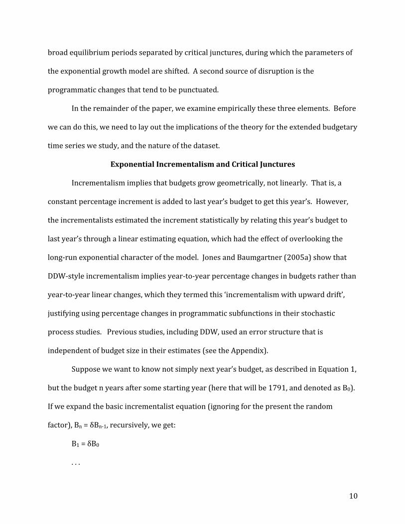
Exponential Incrementalism and Critical Junctures

Incrementalism implies that budgets grow geometrically, not linearly. That is, a

constant percentage increment is added to last year’s budget to get this year’s. However,

the incrementalists estimated the increment statistically by relating this year’s budget to

last year’s through a linear estimating equation, which had the effect of overlooking the

long-run exponential character of the model. Jones and Baumgartner (2005a) show that

DDW-style incrementalism implies year-to-year percentage changes in budgets rather than

year-to-year linear changes, which they termed this ‘incrementalism with upward drift’,

justifying using percentage changes in programmatic subfunctions in their stochastic

process studies. Previous studies, including DDW, used an error structure that is

independent of budget size in their estimates (see the Appendix).

Suppose we want to know not simply next year’s budget, as described in Equation 1,

but the budget n years after some starting year (here that will be 1791, and denoted as B0).

If we expand the basic incrementalist equation (ignoring for the present the random

factor), Bn = δBn-1, recursively, we get:

B1 = δB0

. . .

11

Bn = δBn-1 = δ(δ)(δ)…(δ)B0 = δnB0

This is a geometric series, the discrete form of exponential change (δ <>1), and

clearly path-dependent in the self-reinforcing sense. Incrementalist budgeting, properly

understood, implies exponential budgetary growth.

Existing budgetary models apply to changes in the levels of budgetary allocations to

programs, yet the size of government changes as a consequence of the addition or

subtraction of entire programs as well as through allocations to existing programs. As a

consequence, we assume that the parameter estimate for the growth factor, δ, is a weighted

average of δs for agencies operative in the nth year. As programs are added or subtracted

to the mix of governmental responsibilities, the number of agencies over which the

weighted average is taken changes.

We define a budgetary equilibrium as a period in which the parameters for

exponential incrementalism remain constant; that is, the budget grows at a constant

exponential rate, and deviations from that rate return to the exponential path. Critical

junctures disrupt a budgetary equilibrium, but following the critical juncture negative

feedback processes stabilize the process such that the parameters remain constant during

the next budgetary era. These negative feedback processes need not, however, restore the

parameters of the previous era.

Because we expect the series to experience major destabilizations from critical

junctures, we seek to isolate periods of stability within which exponential incrementalism

holds in the budget data series. We isolate budgetary eras divided by critical junctures

both statistically and historically, and then we examine the constancy of the parameters

during the eras. Finally, we examine the residuals from our estimates for the exponential

12

path during the equilibrium periods to see if the deviations are smaller than those of a

distribution of the full-length budget changes. This would indicate whether critical

junctures are a necessary component of a long-run budget theory.

Constructing the Data Series

We encountered considerable difficulties in constructing a satisfactory budget series

for the US government to estimate exponential incrementalism. Long-term data for

agencies or budget categories do not exist in any form, forcing investigators to rely on

outlays. Two separate sources must be used to construct a series for overall outlays for

the full period (one compiled by the Treasury Department, 1791-1970; the other by the

Office of Management and Budget, 1940-2010). These sources are consistent for overall

outlays, but not for categories of spending. In the Treasury series, outlays are broken

down only for domestic and defense, but the OMB series reports finer grained categories.

Our analysis of the overlap period indicated that the two systems of categorization were

not entirely consistent. As a consequence, we constructed two separate synthetic series

from the two separate sources, and performed robustness tests to see if the differences

might affect our findings. The series were adjusted for inflation before analysis. Full

details are contained in the on-line appendix; we have also made the data available for

download through the Policy Agendas Project (http://www.policyagendas.org/).

Estimating Exponential Incrementalism

Exponential growth in expenditures implies linear growth in the logarithm of

expenditures over time (see the Appendix for details). So the estimating equation for the

logarithm of the expected budget is

lnB t = lnB0 + λt = A0 + λt [Equation 3]

13

This simple log-linear growth pattern would result from the fully isolated, closed

budgetary system, but the simple formulation is clearly unrealistic. External factors can

disrupt the internally-dominated, closed incremental system. These external factors have

two separate potential effects: they may ratchet expenditures up or down from the

fundamental exponential path, shifting the magnitude of Ao, or they may shift the velocity,

or incremental growth parameter, estimated by slope, , making it steeper or flatter.

Shifts in the intercept, Ao, are consistent with the general theory developed here so

long as the shifts are directly associated with critical moments and if the periods between

the shifts are stable—statistically as well as substantively. Discrete shifts in the

exponential velocity, , can also occur; if they are associated with critical moments they are

also consistent with the general theory articulated here.

Our predictions from the general theory will be supported by the analysis if a model

of exponential incrementalism holds except at critical junctures. At these critical

junctures, either A0 the exponential intercept, or λ, the exponential velocity, or both may

change. The periods between the critical junctures should be stable, both substantively and

statistically. Minor destabilizations in which there is a reasonably rapid return to the

stable exponential path are consistent with the theory. Situations in which local

destabilizations occur, but the system returns to the previous exponential trend rapidly,

provide evidence that the path-dependent process is resilient, and hence are consistent

with the predictions.

The model would not be sustained if parameter shifts occur in circumstances not

associated with crises (else the term path dependency has little meaning) or if the data do not fit

exponential incrementalist model for extended periods. Exponential incrementalism would be

14

rejected should the logarithm of budgets curve upward (in which case budgets would be

growing faster than exponential), or downward (in which case budgets would be growing

slower). Such a pattern implies that the system is continuously adjusting off the

exponential path. A self-reinforcing path dependent budgetary process may be subject to

destabilization in crises, but it should not be subject to on-going more minor cumulative

destabilizations implied by the flow of information.

The difference between a linear understanding of budget changes and an

exponential one is non-trivial. If a budget started at a base of zero, and was subject to a

linear aggregation of .03 million dollars each year, at the end of a decade the budget would

be $333,000. If it were aggregated geometrically, with the budget incremented 3%

annually, the government’s budget would be $1,350,000. If, during a critical juncture, the

budget exponent increased to 4%, the exponential incremental budget would be

$1,490,000. This difference would continue to grow, and by a quarter of a century the

budget incremented by .03 would have aggregated to $2,117,000, while the budget

incremented by .04 would be $2,720,000. The linearly aggregated budget would have

aggregated only to $750,000.

A First Look at the Historical Pattern

In Figure 1, we plot the logarithm of real expenditures for the period 1791 through

2010. It is clear that the growth pattern is largely exponential, but major deviations occur.

The deviations seem to be of two types. The first consists of spikes associated with major

wars (the Civil War and the two World Wars), and involve both sharp changes associated

with mobilization and with de-mobilization at the end of the war. Note that in every case

15

the level of government spending does not return to pre-war levels. Rather they stabilize

at a level considerably above the previous level.

Figure 1: Logarithm of US Expenditures, 1791-2010

16

Note: The top panel depicts the full historical period, while the bottom panel depicts the post-

1950 period. The growth path for US expenditures is exponential, but major deviations occur.

Especially noteworthy are the three abrupt ratchets and the distinct curvature after 1980.

The second type of deviation from the strict exponential path involves changes in the

exponential slope. Changes in slopes seem to occur after the wars. After the Civil War, the

slope flattens out; between the two World Wars, the slope sharply increases; after the

Second World War, the slope decreases (and, indeed, exhibits a pronounced deceleration).

A closer examination shows that this budgetary deceleration occurred in the period from

around 1986 to 2001, with exponential growth resuming afterward. This was the period

in which stringent budgetary ‘pay-go’ rules were in effect, and suggests problems with our

predictions.

Statistical Approaches

While it is clear that the general path of US expenditures has been exponential, there

are a number of spikes, twists, and turns that characterize budget development. We

examine the extent to which deviations from the exponential trend act as destabilizations

that tend to return to the fundamental exponential path, or whether those destabilizations

result in a) permanent ratchets, b) permanent changes in the rate of growth (slope

changes); or c) changes away from the exponential path.

In analyzing the trend, we apply two distinct approaches. Method 1 is a smoothing

technique applied to the budget series by taking the cumulative sum of the budget values—

roughly the numerical integration of these values--allowing us to focus on the main trends

in the data. We may think of this as kind of bird’s-eye view of the budget process. We fit

17

least squares models to the stable periods indicated by an examination of the graphs.

Method 2 is an examination of rates of change instead of budgetary levels, again seeking

deviations from the hypothesized exponential path. More specifically, we analyze the

logarithm of year-to-year change ratio, log(B(t)/B(t-1)); we refer to this as the derivative of

the logarithm of the budget. We fit several least-squares trend line models to the full

budget series for this measure, distinguishing between them using two standard

procedures, Bayesian Information (BIC) and Akaike Information Criteria (AIC). The

derivative of the log budget indicates the behavior of budget adjustment to the trend, while

log budget integral reflects the trend itself.

Method 1: Exponential Trend Analysis

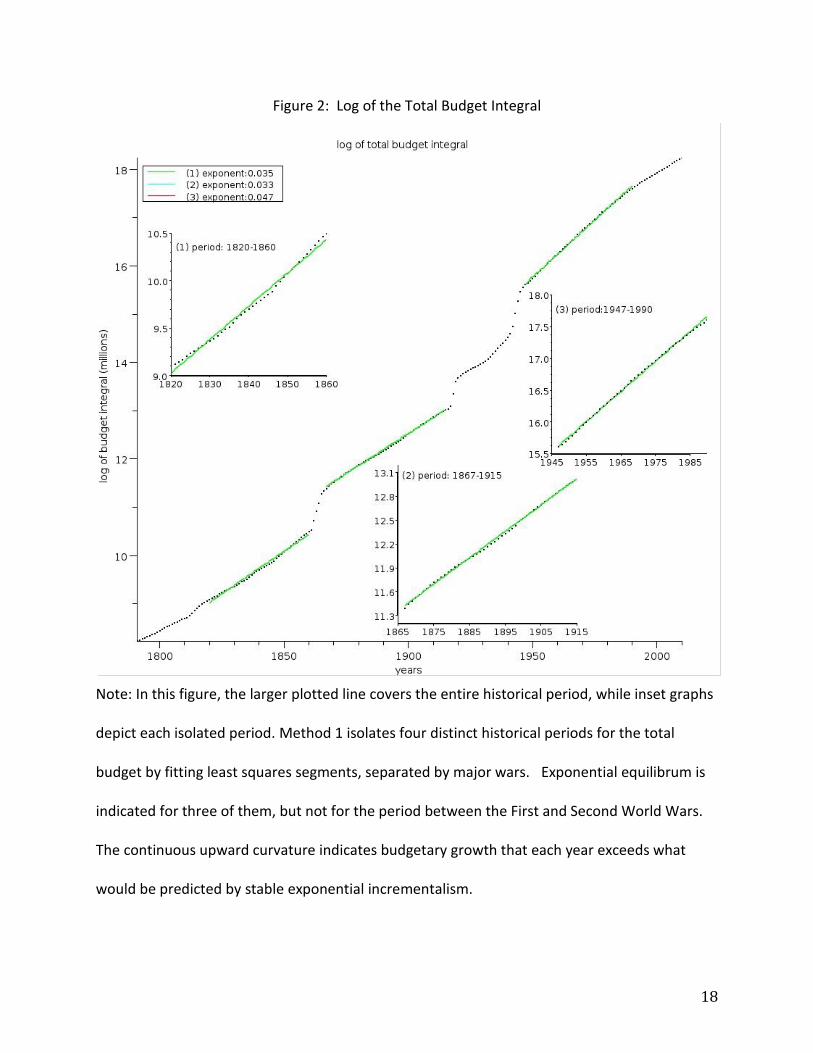
Method 1 examines the cumulative sum of the budget values—roughly the

numerical integration of the series. If the trend is exponential, its integral will be too.

(Details may be found in the on-line appendix.) Taking the logarithm of the budget integral

would produce a linear plot, and Figure 2 does this. The figure shows the full series, along

with parts of the sub-series that were long enough to calculate stable least squares

estimates. The approach isolates four different segments, with the break points delineated

by wars, three of which were stable. The period between WWI and WWII distinctly curves

upward, indicating an annual adjustment process that is not consistent with pure

exponential incrementalism. The corresponding least-squares estimators in the box at the

top left of the figure. The solid lines delineate the portions of the curve for which we were

able to calculate stable estimates (1820-1860; 1867-1915, and 1947-1990).

18

Figure 2: Log of the Total Budget Integral

Note: In this figure, the larger plotted line covers the entire historical period, while inset graphs

depict each isolated period. Method 1 isolates four distinct historical periods for the total

budget by fitting least squares segments, separated by major wars. Exponential equilibrum is

indicated for three of them, but not for the period between the First and Second World Wars.

The continuous upward curvature indicates budgetary growth that each year exceeds what

would be predicted by stable exponential incrementalism.

19

The Civil War seems to have had two effects: it resulted in a permanent upward shift

in the level of expenditure, and it led to a period of slower growth in the budget (as

assessed by a decline in the exponential exponents from 0.041 to 0.034). One source of

this upward shift is the fiscal burden of military pensions and funds for war widows and

orphans. The period from the Civil War to the First World War was a period of remarkably

stable budget growth—exponential growth, but at relatively lower rate compared to what

came before and what came afterward. The First World War resulted in, again, a

permanent shift in level of expenditure, and a clear upward shift in slope, associated with

the New Deal response to the Great Depression. In this case, however, it was not possible

to secure a stable estimate of the slope because of the continual adjustment process that

results in increases that are faster than exponential after around 1930. The Second World

War generated the expected upward shift in level, and a lower rate of growth (compared to

the Inter-War period). But the rate was greater than the 1865-1915 period, as indicated by

an exponent of 0.0473.

Domestic and Defense

Our data series allow us to analyze patterns of change for domestic and defense

outlays separately. We performed the same Method I analyses on each that we did for the

total budget, and the results are presented in Figures 3 and 4. Our analyses of the log of the

budget integral for the case of defense outlays isolated five different segments, which were

similar to those isolated for the total budget, with two exceptions. The 1865-1915 interval

for defense decomposed into two parts, before and after 1900; there is an accelerated

growth after this point. The break may be associated with President Theodore Roosevelt’s

expansionist foreign policy (Holmes 2006). In any case, it is hard to associate this shift in

20

slope with any ‘critical juncture’ in the environment, yet the shift had a considerable effect

on budgetary outlays. In addition, the period between the world wars was stable and could

be estimated.

For the domestic outlays the descriptive path of isolated by the log of the budget

integral is not as clear, as there exist periods in which growth is not exponentially stable.

The most interesting two segments are at the beginning and at the end of the 20th Century.

In both cases, domestic spending growth decelerated for an extended period of time. We

discuss the latter deceleration later in the paper. These decelerations (or accelerations)

indicate difficulties with the theory, since they imply an internal adjustment process that is

not abrupt and is not associated with crises or ‘critical moments’. However if these

changes are also associated with non-Gaussian processes in the residuals around the

exponential path, then they may be associated with programmatic punctuations found in

the policy process studies.

21

Figure 3: Log of Budget Integral for Defense Outlays

Note: The larger plotted line covers the entire historical period, while inset graphs depict each

separate period. Method 1 isolates five historical periods for the defense budget, similar to the

overall budget analysis of Figure 1 with two exceptions. Both are shifts in the exponential

slope, one associated with President Theodore Roosevelt’s military expansion in around 1900,

and the other with a post-Vietnam withdrawal of military expenditures.

22

Figure 4: Log of Budget Integral, Domestic Outlays

Note: The larger plotted line covers the entire historical period, while inset graphs depict each

separate period, using Method 1. There are periods in which exponential growth seems not to

be exponentially stable for the domestic budget.

Method 2: Rates of Change

Method 2 examines rates of change instead of budgetary levels. Figure 5 displays

the year-to-year budget change ratio (proportion change) and the logarithm of the budget

23

change ratio.

Figure 5: Annual Budget Change Ratios

Note: Method 2 focuses on year-to-year budget changes instead of the absolute budget

amounts of Method 1. Figure 5 presents the general picture. We examine the logarithms of

the budget ratios of one year’s expenditures to the previous year’s expenditures, as implied by

our theory.

24

Using a systematic process, we fit various least-squares trend line models to the full

derivative of the log budget series. (Details may be found in the on-line appendix.) Were

exponential incrementalism the only explanation for budget change, a single line segment

with near-zero slope would be satisfactory. But this is clearly not the case. As the number

of lines fit to the series increases, the error in the fit decreases, so we use standard model

fit criteria that adjust for the number of parameter estimates (Bayesian Information and

Akaike Information Criteria) to judge fit. Figure 6a shows the model fit statistics (BIC and

AIC), plotted against the number of line segments fitted. The goodness of fit statistics help

find the optimal balance between the number of parameters and model fit to avoid

overfitting the data. We also examine points at which large drops occur in the statistics,

indicating large improvements in model fit. The graph of the criteria indicates a large drop

at six line segments, and again at eleven, with only incremental model improvements after

that. Figure 6b shows least-squared estimates of the log budget derivative for eleven

segments.

25

Figure 6a: The Number of Least Square Segments Plotted Against AIC and BIC.

Note: Method 2 fits least squares segments to the budget change ratios in Figure 6 through an

algorithm. Figure 6a depicts changes in the model goodness of fit statistics. While the

goodness of fit statistics are going down as the number of line segments increases, model fit is

improving. When it levels out, no further improvement occurs.

26

Figure 6b: Least Squares Fit of the Derivative of the Logarithm of Expenditures with Different Line Segments

Note: This figure depicts the line segments fit according to our algorithm, from two segments to

thirteen. Best fits, according to Figure 6a, are for six and eleven line segments.

Whether six or eleven line segments are fitted, the general form of the series

remains similar to that fitted using the log integral method in Figure 2. The approach

isolates three periods of stability interrupted by large spikes due to war mobilization and

demobilization (these are approximately the same periods as were isolated using the log of

the budget integral in Figure 2). These periods experienced steady growth in the budget,

but the first period experienced quite high levels of year-to-year variability. It also detects

27

a line segment corresponding to the inter-war years and the Great Depression with a clear

upward shift in slope from the pre-WWI period. During this period, the rate of change was

growing steadily—basically a longer period of non-equilibrium than the war spikes

(Jánossy 1971).

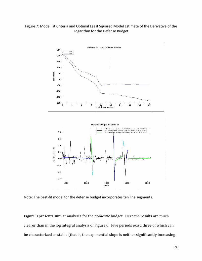
Figure 7 presents the derivative of the logarithm of the defense budget Figure 7a

presents the model goodness of fit statistics (AIC and BIC), which indicate a best fit of ten

segments. Figure 7b presents the best-fit model estimate. The results generally confirm

the findings from Figure 5, the slopes based on the log integral analysis.3

3 There are some differences in the periods isolated by the two methods. Most importantly, the log

integral defense plots isolates two segments for the 1867-1915 period, whereas the derivative of

log budget method does not. This is because the two methods are sensitive to different aspects of

budget change: the integral shows the average increase while the derivative of log budget is

sensitive to the immediate change.

28

Figure 7: Model Fit Criteria and Optimal Least Squared Model Estimate of the Derivative of the Logarithm for the Defense Budget

Note: The best-fit model for the defense budget incorporates ten line segments.

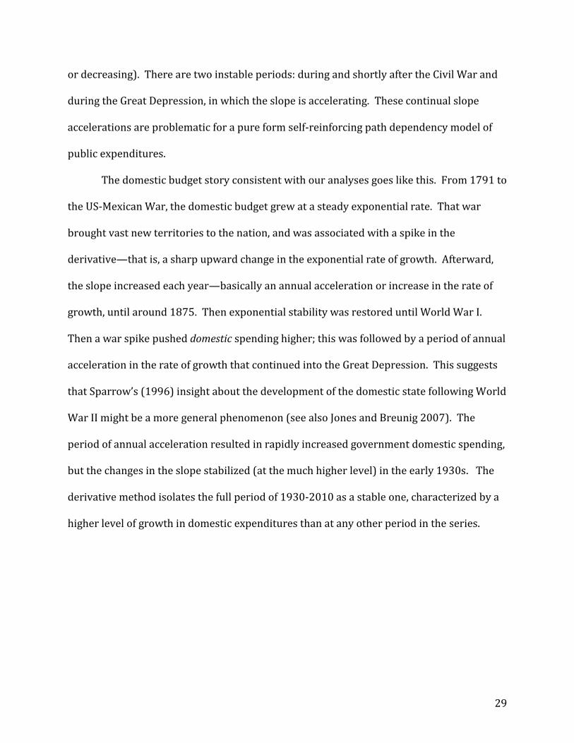
Figure 8 presents similar analyses for the domestic budget. Here the results are much

clearer than in the log integral analysis of Figure 6. Five periods exist, three of which can

be characterized as stable (that is, the exponential slope is neither significantly increasing

29

or decreasing). There are two instable periods: during and shortly after the Civil War and

during the Great Depression, in which the slope is accelerating. These continual slope

accelerations are problematic for a pure form self-reinforcing path dependency model of

public expenditures.

The domestic budget story consistent with our analyses goes like this. From 1791 to

the US-Mexican War, the domestic budget grew at a steady exponential rate. That war

brought vast new territories to the nation, and was associated with a spike in the

derivative—that is, a sharp upward change in the exponential rate of growth. Afterward,

the slope increased each year—basically an annual acceleration or increase in the rate of

growth, until around 1875. Then exponential stability was restored until World War I.

Then a war spike pushed domestic spending higher; this was followed by a period of annual

acceleration in the rate of growth that continued into the Great Depression. This suggests

that Sparrow’s (1996) insight about the development of the domestic state following World

War II might be a more general phenomenon (see also Jones and Breunig 2007). The

period of annual acceleration resulted in rapidly increased government domestic spending,

but the changes in the slope stabilized (at the much higher level) in the early 1930s. The

derivative method isolates the full period of 1930-2010 as a stable one, characterized by a

higher level of growth in domestic expenditures than at any other period in the series.

30

Figure 8: Model Fit Criteria and Optimal Least Squares Fit of the Derivative of the Logarithm for Domestic Expenditures

Note: For the domestic budget, Method 2 isolates five historical periods, three of which are

stable. During the two periods not characterized by a stable exponential slope, 1850-1865, and

between the First and Second World Wars, the rate of growth increases each year.

Comparing the Two Methods

The analysis of the change of log-budgets complements the log integral method, but

the two approaches yield some important differences. The derivative of log budget method

31

identifies the stable periods but is not sensitive to steady changes in the growth rate. For

example in Figure 3, in the middle section of the defense budget (1865 to WWI) there are

two periods with different growth rates on the log integral graph reflecting a steady

(stable) change in expenditures. The change in slope is small compared to the fluctuations

and hence it is detected as a single stable period by the derivative of log budget method

(Figure 7).

Similarly, while the derivative method lumps the period after WWII as a single era,

the log integral method reveals the existence of the period of budget deceleration that

occurs from 1988-2000. While this period of deceleration proved fleeting, its existence is

important, since it indicates that internal dynamics can ‘bend the budget curve’ through the

application of budgeting procedures. These findings are problematic for our theory based

on a pure path dependent budgetary system, because it is hard to argue that the budgetary

struggle of the 1980s and early 1990s was anything more than politics as usual.

For both methods, we find that wars destabilize both defense and domestic budgets,

but with somewhat different effects. Wars basically ratchet up defense spending, and do

not affect the exponential rate of growth. But they tend to affect domestic spending by

altering the exponential rate of growth, with a much more muted ratchet effect. Defense

budgets are affected by the mobilization needs associated with war, but demobilization

also tends to occur and a new growth factor need not be built into the system. For

domestic expenditures, however, statutory changes tend to perpetuate themselves,

resulting in changes in the domestic spending growth slope.

Fluctuations Around the Trend

32

We have thus far analyzed historical budget macro-behavior using two measures,

the log budget integral and the derivative of the log budget. We isolated three major

budgetary periods using these methods, and these budgetary periods correspond to that

predicted by the historical record. Now we examine the behavior of the observations

within these three equilibrium periods. We examine the residuals for each period for

normality, for randomness, and for stationarity.

If we return to the now-common stochastic process approach for analyzing

budgetary changes, and studied frequency distributions for the US budget from 1791 to

2010, we would find it easy to reject the simple linear incremental model. For annual

budget changes for the defense budget, the kurtosis is 56.9, for the domestic budget, 41.0.

We could also reject exponential incrementalism, even if not so dramatically: for frequency

distributions of the logarithm of budget changes, the kurtosis for the total budget is 17.3,

for the defense budget 11.8, and for the domestic budget, 15.6. The distributions are

shown in Figure 9.

Figure 9: Histogram of the Logarithm of Budget Changes for the Full Data Series (1791-2010) for Defense, Domestic, and the Total Budget

33

Note: The figure shows budget change data (in logarithms) for the full dataset. The data exhibit

the clear leptokurtic pattern associated with policy process studies. If the critical junctures

make little difference in budgetary dynamics—that is, if critical junctures are just part of a

broader budgetary dynamics that characterizes the whole budgetary series, then we expect

frequency distributions examining only the distributions for the stable periods to resemble

these distributions.

But we have mixed equilibrium periods with critical junctures. What happens if we

focus only on the residuals within the equilibrium periods? Focusing only on these three

stable periods, we examined the residuals from the fitted least squares line for the

derivative of the log of the budgets, with the results presented in Figure 10. The periods

show different distributions clearly with different standard deviations, skewness and

kurtosis, strengthening our previous findings of different budgeting eras throughout the

years. The residuals are the random adjustments to the general trends; to verify the

hypothesis of exponential incrementalism the residuals must be noise.

During the first two periods, defense spending is more punctuated (that is, with

higher kurtosis), while domestic spending approaches normality. In the last period, after

World War II, the relative roles are reversed, with domestic spending more punctuated and

defense spending more normal. The destabilizations in domestic policy in the post-war

period are more abrupt than in the previous periods, and are more abrupt than defense

spending. This could be a consequence of the addition of new domestic programs and

subsequent cutting of them at a level unprecedented in earlier periods. The finding

34

dovetails with stochastic studies of changes in budget allocations across programs, all of

which focus on the post-war period.

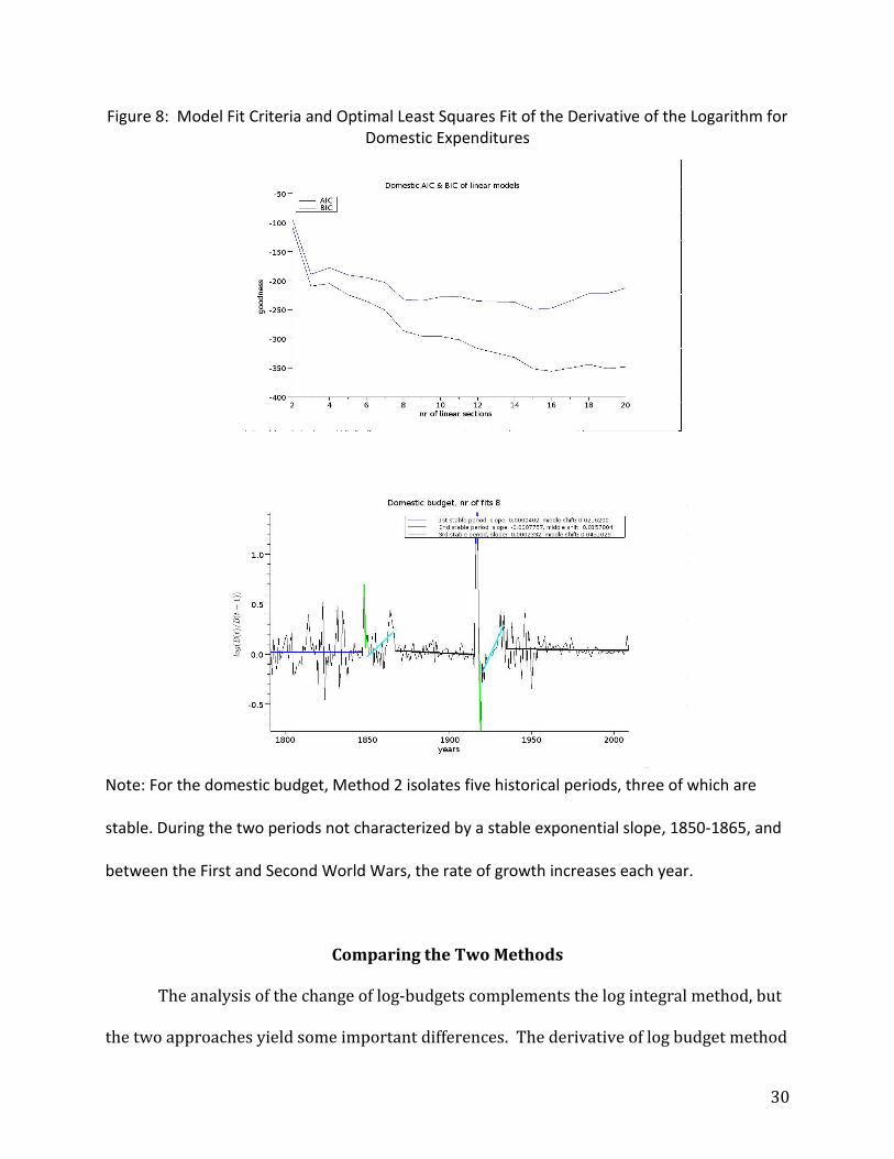
Figure 10: Residuals from Fittings to the Derivative of Log Budget of Stable Periods

Total

Defense

35

Domestic

Note: The figure displays the residuals of the least squared fits for the three stable periods,

displayed as frequency distributions. The distributions are presented separately for the Total,

Defense, and Domestic Budgets. Compared to the full series analysis presented in Figure 9, the

histograms have fewer cases in the tails, and the kurtosis, which assesses punctuations in

change data series, is reduced. This indicates a need for incorporating critical junctures into

the theory. But for some periods the kurtosis remains large, indicating budget punctuations

within the stable period.

Randomness

We used the Lilliefors test to determine if the residuals from the least squared

fittings have Gaussian distributions for the stable periods. We found that total and defense

budget for the last period and domestic spending for the first two series are accepted as

Gaussian distribution at 5% significance level. In Figure 9 the skewness and kurtosis of the

first and second periods also support these findings.

If we re-examine Figure 4, we see that there is a break for defense spending around

1900. If we split the middle period of defense spending into two parts as Figure 4 suggests,

36

the test accepts the Gaussian hypothesis for the residuals again. The same holds for

domestic outlays: taking the residuals from 1951 to 1990, leaving out the post crisis and

wartime parts yields normally distributed residuals.

We then tested the independence of the three successive samples of residuals to see

if they could be viewed as independently drawn and identically distributed. A Ljung-Box

test indicated the independence of the autocorrelation coefficients for the first two stable

but not for the last period. The total budget residuals show independence, so domestic and

defense budget are independently determined—that is, they seem to be driven by distinct

dynamics.

Stationarity

The natural assumption is that at least within the stable periods the adjustment

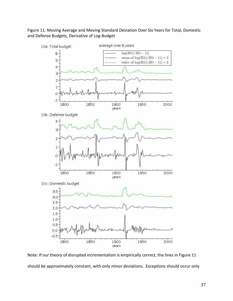
process is homogeneous, and the random process is stationary. Figures 11 and 12 present

stationarity tests for the stable periods with two different methods: moving average and

standard deviation and the sum of deviations. The former approach indicates that the

middle and last periods are stationary in a weak sense for the total budget. The domestic

budget during WWII, where the large periodic oscillation appears, is an exception, but

stationarity holds afterwards. Interestingly the first period seems not to be homogeneous,

and both mean and standard deviation jump up and down. At the jumps there are smaller

scale wars and other factors that come into play. We conclude that these situations

temporarily increase the fluctuation but soon disappeared, leaving no real effect on the

budgeting system.

37

Figure 11: Moving Average and Moving Standard Deviation Over Six Years for Total, Domestic and Defense Budgets, Derivative of Log-Budget

Note: If our theory of disrupted incrementalism is empirically correct, the lines in Figure 11

should be approximately constant, with only minor deviations. Exceptions should occur only

38

during critical junctures, which should show up as large deviations. This is true for the middle

and late periods for the total budget, but not for the first period. But these deviations do not

seem to have effects on the total budget path.

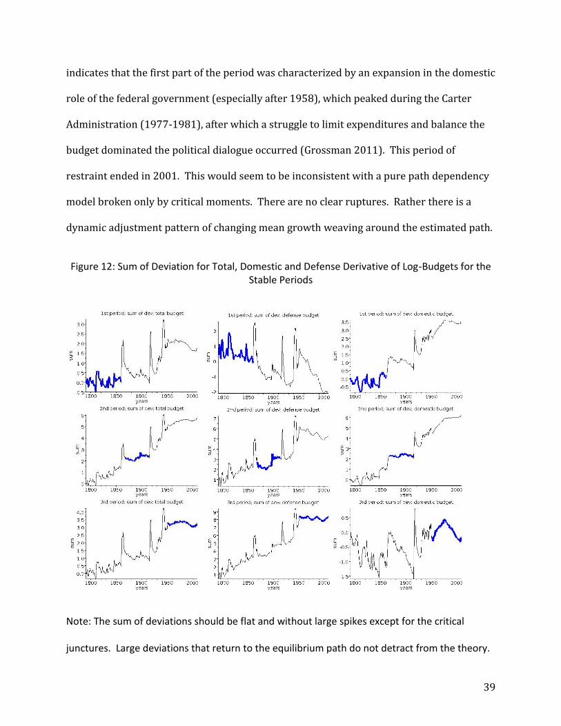
The sum of deviation method identifies a potential change in the mean exponential

slope. The fluctuations are too large compared to the data length to gain clear results of

changes in the mean during these stable periods. However the method shows that the most

stationary period is the middle period (for both total and domestic) but also shows that

there is an unbalanced shift in the defense budget. This indicates a changed mean

exponential slope that occurred around 1900, which is consistent with what we found

using the log integral method. Historically increasingly muscular foreign and defense

stance, represented by the actions of President Theodore Roosevelt characterized this

period.

The graphs of the last panel in Figure 12 offer further support that the pure path

dependency model is an incomplete model for budgetary dynamics. The most interesting

element is the clear roof-shape change in the sum of the deviations for domestic spending,

hidden in the moving average method. The sum of the deviations for domestic spending

grew during the post-WWII period until around 1975, and then they began to shrink.

Looking at Figure 8, we can see that there was one big oscillation, with the deviations

mostly in the positive direction (that is, there were increases in the slope spending relative

to the estimated mean path), and then after 1975, there were decreases in the slope. The

pattern is consistent with historical and documentary evidence. The historical record

39

indicates that the first part of the period was characterized by an expansion in the domestic

role of the federal government (especially after 1958), which peaked during the Carter

Administration (1977-1981), after which a struggle to limit expenditures and balance the

budget dominated the political dialogue occurred (Grossman 2011). This period of

restraint ended in 2001. This would seem to be inconsistent with a pure path dependency

model broken only by critical moments. There are no clear ruptures. Rather there is a

dynamic adjustment pattern of changing mean growth weaving around the estimated path.

Figure 12: Sum of Deviation for Total, Domestic and Defense Derivative of Log-Budgets for the

Stable Periods

Note: The sum of deviations should be flat and without large spikes except for the critical

junctures. Large deviations that return to the equilibrium path do not detract from the theory.

40

But in two places there are problems: for the defense budget around 1900 and for the domestic

budget after the early 1950s.

We cannot strongly justify stationarity of the stable sections, so there are indications

of possible changes in the stochastic processes. It is likely that some of short-term effects

are explained by strong but localized influences on the budgetary processes. Again, this

conflicts with important predictions from the theory.

Summary and Implications

In this paper, we detailed a general theory of budgetary dynamics over long time

periods. The theory is based on three elements from the current literature on the politics

of the budgetary process. From decision-making theories, we derived the implication of

exponential growth in budgets. From the general notions of path dependency and critical

junctures, we inferred that the parameters for the exponential growth model would be

constant only for the periods between the critical junctures. From policy process theories,

we drew the concept of programmatic punctuations.

The basic driver of budget change in the US over the long run is a self-reinforcing a

recursive incremental system whose solution is exponential growth, termed exponential

incrementalism. Each year the budget base is multiplied by a built-in growth factor, the

budget increment: B = Boexp(t), where B is the budget in a given year, Bo is the starting-

point, is the constant exponent, and t is the number of years since Bo. The budget

increment comes both from the classic incrementalist dynamic of adding to existing

programs and from the addition of new programs over time.

41

We hypothesized that this model would hold only for periods within historically

important critical junctures: major wars and the Great Depression. Tests of this model on a

newly constructed data series of US expenditures since 1791 show that the model

characterizes three major periods of budget stability in American history characterized by

consistent year-to-year growth in total expenditures (1790-1860; 1865-1915, and 1950-

2010). The critical junctures separating the equilibrium periods were characterized by

changes in the budget intercept, Bo, the budget increment , or both.

Some aspects of the analysis are problematic for the model. These are periods of

changes in the velocity of exponential growth—basically the acceleration is not constant.

For Method 1 these are indicated by changes in linearity, and for Method 2 by changes in

constancy. An upward bending Method 1 curve implies that the growth rate is accelerating,

while a downward-bending curve indicates deceleration in comparison to exponential

growth. A clear upward-bending curve, particularly in evidence for the total budget

analysis, occurs between the First and Second World Wars (see Figure 2). For domestic

expenditures, an upward bending of growth velocity occurs between the 1850 and 1865,

and downward bending curves occur between 1900 and World War I and during the 1980s

and 1990s. The pattern after WWII seems to be constituted of two distinct periods. The

first, from the War to the late 1970s, was a period of aggressive government growth (recall

that the rate of exponential growth was higher than in any other stable period). This was a

result of the aggressive addition of new programs during the late 1950s to the mid 1970s.

The second period was one of annual deceleration off the exponential path. This was likely

driven by changes in the allocation rules, as the Gramm-Rudman-Hollings and Pay-Go

budget rules to limit deficits took hold. These were not renewed when G.W. Bush took the

42

presidency, resulting in a restoration of the previous growth path.

The three periods for domestic expenditures (approximately 1850-1865, 1900-

1915, and 1980-2000) are off the equilibrium path, and are inconsistent with exponential

incrementalism and hence self-reinforcing path dependency. They are likely associated

with political forces that affect the growth path, pushing expenditures upward or

downward from the built-in path dependent equilibrium for a number of years.

When we studied the behavior of residuals within the periods of stability we found

further evidence of deviations from a pure path dependency model. Within periods of

stability our stationarity tests suggest a complex within-period adjustment pattern. Even

below the surface, considerable churning occurs, as particular programs lose and gain favor

with policymaking officials. The equilibrium periods are best characterized as ‘noisy

equilibria’ in which deviations from the exponential growth path tend to return to the

existing path, but not always immediately. Even during the stable periods, important

short-term dynamics can influence the rapid return to the exponential equilibrium. This

could involve ‘minor’ wars and the challenges of integrating new territories into the nation,

as was the case in the 1850s, or other localized but important forces.

The policy process approach to budgeting, with its reliance on resistance and

friction in policymaking institutions, implies that the budgetary path is disjoint and

episodic, and hence annual budgetary changes would be subject to higher kurtosis values,

implying leptokurtosis, while skewness remains within the bounds of Normality. We found

this to be true in important instances, particularly for domestic expenditures in the post

World War II period.

43

In sum, we find support for the general theory of budgeting, but some contrary

results as well. We find two forms of inconsistencies with the model: changes in the

exponential slope over a period of years, and deviations within some of the stable periods

that indicate oscillations in the exponential slope. The deviations from a pure path

dependent budgetary model we have uncovered suggest that internal adjustments can

affect budgetary path dependency in the absence of the large destabilizing forces of critical

moments.

One might like to have more certainty in the confirmation or disconfirmation of a

theory. But in the real world of incomplete theories, human agency, and noisy historical

data, that is not in the cards. We can say that major elements of the theory are confirmed,

including the general dominance of exponential incrementalism, the role of critical

junctures, and the punctuated behavior during the stable periods. But at times local

political forces can influence outcomes. Perhaps most importantly, we have extended our

understanding of budget dynamics by developing a comprehensive framework that

subsequent studies can address.

Nevertheless, there seems to be important historical contingencies that affect

budgetary politics. The general theory seems less valid during the last, Post World War II

historical period. The budget path clearly bends in a manner not consistent with pure

exponential incrementalism (see Figures 1-4). And there is considerably more disjoint

change in the residuals for the period (see Figure 10). With the addition of many new

government programs, budgeting is far more complex today than in the past. This seems to

have generated a budgetary politics that is both more complex and less likely to fit the

44

theory. This evolutionary component of government development is worth further

research.

45

References

Bacaer, Nicolas. 2011. A Short History of Mathematical Population Dynamics. London:

Springer.

Begg, Iain. 2007. The 2008/2009 EU Budget Review. EU-Consent EU-Budget Working

Paper #3.

Bertalanffy, Ludwig von. 1968. General System Theory: Foundations, Development,

Applications

Breunig, Christian and Bryan D. Jones. 2011. Stochastic Process Methods with an

Application to Budgetary Data. Political Analysis 19: 103-17.

Breunig, Christian, and Chris Koski. 2012. The Tortoise and the Hare: Incrementalism,

Punctuations, and Their Consequences. Policy Studies Journal 40: 45-67.

Capoccia, Giovanni, and R. Daniel Kelemen. 2007. Critical Junctures: Theory, Narrative,

and Counterfactuals in Historical Institutioanlism. World Politics 59: 341-69.

Carpenter, Daniel. 1996. Adaptive Signal Processing, Hierarchy, and Budgetary Control in

Federal Regulatory Agencies. American Political Science Review 90: 283-302.

Davis, Otto A., M.A.H. Dempster, and Aaron Wildavsky. 1966. A Theory of the Budget

Process. American Political Science Review 60: 529-47.

Davis, Otto A., M.A.H. Dempster, and Aaron Wildavsky. 1974. Towards a Predictive Theory

of Government Expenditure: US Domestic Appropriations. British Journal of Political

Science 4: 419-52.

46

Dufour, Caroline. 2008. The Format of the Expenditure Budget of the Government of

Ontario: A Path Dependent Model. Vancouver, BC: Paper presented at the Annual

Meeting of the Canadian Political Science Association.

Érdi, Peter. 2008. Complexity Explained. Berlin: Springer.

Grossman, Matthew. 2011. “American Domestic Policymaking Since 1945: The Aggregate

View from Policy History.” at the Midwest Political Science Association Annual

Meeting. Chicago, IL. April 2011.

Holcombe, Randall G. 2005. Government Growth in the 21st Century. Public Choice 124:

95-114.

Holmes, James. 2006. Theodore Roosevelt and World Order. Washington DC: Potomac

Books.

Howlett, Michael and Andrea Migone. 2011. Charles Lindblom Is Alive and Well and Living

in Punctuated Equilibrium Land. Politics and Society 30: 53-62.

Howlett, Michael and Jeremy Rayner. 2006. Understanding the Historical Turn in the

Policy Sciences. Policy Sciences 39: 1-18.

Jánossy, Ferenc. 1971. The End of the Economic Miracle. International Arts and Sciences

Press.

Jones, Bryan D. and Frank R. Baumgartner. 2005a. A Model of Choice for Public Policy.

Journal of Public Administration Research and Theory 15: 325-351.

Jones, Bryan D. and Frank R. Baumgartner. 2005b. The Politics of Attention. Chicago:

University of Chicago Press.

47

Jones, Bryan D., Frank R. Baumgartner, and James L. True. 1996. The Shape of Change:

Punctuations and Stability in US Budgeting, 1947-96. Paper presented at the

Midwest Political Science Association, Chicago, IL.

Jones, Bryan D. and Christian Breunig. 2007. Noah and Joseph Effects in Government

Budgets: Analyzing Long-Term Memory. Policy Studies Journal 35: 329-348.

Jones, Bryan D., Tracy Sulkin, and Heather Larsen. 2003. Policy Punctuations and

American Political Institutions. American Political Science Review 97: 151-70.

Jones, Bryan D., et al. 2010. A General Empirical Law of Public Budgets. 2009. American

Journal of Political Science 53: 855-73.

Key, V.O. Jr. 1940. The Lack of a Budgetary Theory. American Political Science Review 34:

1137-

Lewis-Beck, Michael and Tom Rice. 1985. Government Growth in the United States.

Journal of Politics

Mahoney, James. 2000. Path Dependency in Historical Sociology. Theory and Society 29:

507-48.

Myers, Roy. 2011. Path Dependence in the Federal Budget Process. Seattle WA: Paper

presented at the American Political Science Association Meetings, September 3.

Niskannen, William. 1971. Bureaucracy and Representative Government. Chicago: Aldine-

Atherton.

Page, Scott. 2006. Path Dependence. Quarterly Journal of Political Science 1: 87-115.

48

Padgett, John F. 1980. Bounded Rationality in Budgetary Research. American Political

Science Review 74: 354-72.

Padgett, John F. 1981. Hierarchy and Ecological Control in Federal Budgetary Decision

Making. American Journal of Sociology 87: 75-128.

Peacock, Alan T., and Jack Wiseman. 1961[1994]. The Growth of Public Expenditures in the

United Kingdom. 2nd Ed., reprinted. Aldershot, England: Gregg Revivals.

Pierson, Paul. 2000. Increasing Returns, Path Dependency, and the Study of Politics.

American Political Science Review 94: 251-67.

Pierson, Paul. 2004. Politics in Time. Princeton: Princeton University Press.

Sparrow, Bartholomew. 1996. From the Outside In: World War II and the Development of

the American State. Princeton: Princeton University Press..

True, James L., Bryan D. Jones, and Frank R. Baumgartner. 1999. Punctuated Equilibrium

Theory. In Paul Sabbatier, ed. Theories of the Policy Process. Boulder, Colo:

Westview.

Wanat, John (1974). "Bases of Budgetary Incrementalism." American Political Science

Review 68: 1221 -28.

Whitman, D.A. 1995. The Myth of Democratic Failure. Chicago: University of Chicago Press.

Wildavsky, Aaron. 1964. The Politics of the Budgetary Process. Boston: Little, Brown.

1

Appendix to Accompany

An Integrated Theory of Budgetary Politics and Some Empirical Tests: The US National Budget, 1791-2010

This appendix presents some details about the construction and validation of

the data series used in the analyses, and it addresses several more technical

methodological issues of modeling and testing that involve more extensive technical

elements. It also includes some extended analyses that reinforce the general

conclusions in the paper.

Construction of the Data Series1

As indicated in our paper, there is no single expenditure series for the US

Federal Government since the founding of the Republic. Two separate data series

are available for US Federal Expenditures. These are : Historical Statistics of the

United States: Millennial Edition database TABLE Ea636–643 (compiled by the

Treasury Department); and Office of Management and Budget, Historical Statistics,

Table 3.1(compiled by the Office of Management and Budget). The Treasury Series

runs from 1791 to 1970, and the OMB series covers 1940 to the present. There exist

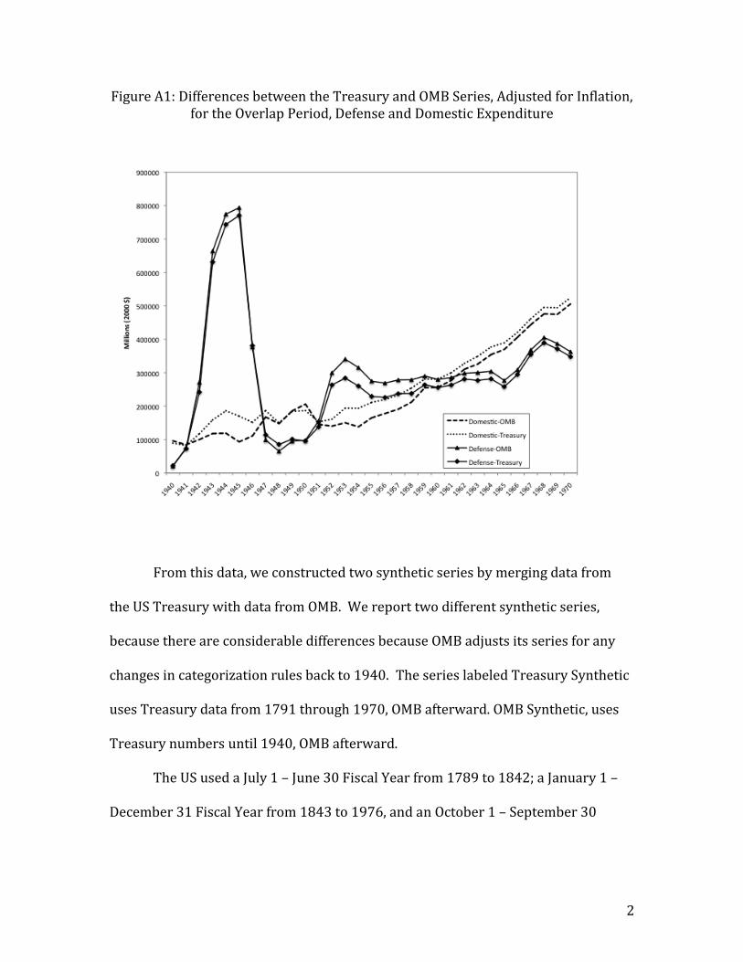
some differences in the two series in the period of overlap, particularly regarding

the Domestic and Defense categorizations. These differences were particularly

severe during WWII and the Korean War. Figure A.1 displays the divergences.

1 We appreciate the efforts of Frank Baumgartner and John Lovett of the University of North Carolina, who were instrumental in the development of the series.

Manuscript ( Not to include ANY author-identifying information)

2

Figure A1: Differences between the Treasury and OMB Series, Adjusted for Inflation, for the Overlap Period, Defense and Domestic Expenditure

From this data, we constructed two synthetic series by merging data from

the US Treasury with data from OMB. We report two different synthetic series,

because there are considerable differences because OMB adjusts its series for any

changes in categorization rules back to 1940. The series labeled Treasury Synthetic

uses Treasury data from 1791 through 1970, OMB afterward. OMB Synthetic, uses

Treasury numbers until 1940, OMB afterward.

The US used a July 1 – June 30 Fiscal Year from 1789 to 1842; a January 1 –

December 31 Fiscal Year from 1843 to 1976, and an October 1 – September 30

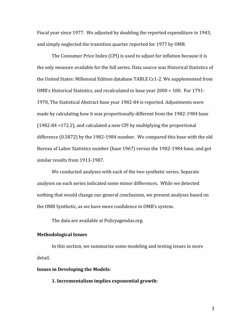
3

Fiscal year since 1977. We adjusted by doubling the reported expenditure in 1943,

and simply neglected the transition quarter reported for 1977 by OMB.

The Consumer Price Index (CPI) is used to adjust for inflation because it is

the only measure available for the full series. Data source was Historical Statistics of

the United States: Millennial Edition database TABLE Cc1-2. We supplemented from

OMB's Historical Statistics, and recalculated to base year 2000 = 100. For 1791-

1970, The Statistical Abstract base year 1982-84 is reported. Adjustments were

made by calculating how it was proportionally different from the 1982-1984 base

(1982-84 =172.2), and calculated a new CPI by multiplying the proportional

difference (0.5872) by the 1982-1984 number. We compared this base with the old

Bureau of Labor Statistics number (base 1967) versus the 1982-1984 base, and got

similar results from 1913-1987.

We conducted analyses with each of the two synthetic series. Separate

analyses on each series indicated some minor differences. While we detected

nothing that would change our general conclusions, we present analyses based on

the OMB Synthetic, as we have more confidence in OMB’s system.

The data are available at Policyagendas.org.

Methodological Issues

In this section, we summarize some modeling and testing issues in more

detail.

Issues in Developing the Models:

1. Incrementalism implies exponential growth:

4

Taking the original incremetalist model (Equation 1) where δ>1 represents

exponential growth and taking the logarithm and expressing the budget with the

starting budget B0: Bn = B0*δn + Σi δi * ηi . The expected value of Bn is B n = B0* δn Þ

lnB n = lnB0 + n*ln(δ). This describes exponential growth with an average slope ln

δ.

2: Some issues with linear estimates of incrementalism.

We have shown that the incremental models were estimated using linear

regression equations, and that the proper approach is geometric growth. The linear

estimating approach actually incorporates assumptions that are incorrect, at least if

followed over a more extended period of time.

One issue is the specification of the error term. The incrementalist models

build in a random error component conceived to be the sum of a series of special

one-time adjustments that behave according to the central limit theorem, and is

assumed to be additive—that is, it is just added to the linear equation. If the budget

is growing by a constant percent, such an error term does not grow in proportion to

the budget. As a consequence, the incremental models imply that the error will

shrink and finally disappear with time—something that obviously can’t happen

given the substantive interpretation. In the original linear model (Equation 1

above), Bn = δBn-1 + ηn implies that Bn/Bn-1 = δ + ηn/Bn-1 . Then ηn/Bn-1 0 as Bn-1

infinity. This is obviously not true.

3. A Note on Exponential Growth

Exponential growth models are an essential component of the study of the

growth of populations. This suggests that students of government size and growth

5

examine some of the basic findings in this field. The ‘pure form’ of exponential

incrementalism presented in this paper would require several assumptions:

assumptions: the system is not destabilized by exogenous events (path dependent,

closed-system incrementalism), and budget growth is not limited by the ‘carrying

capacity’.

The meaning of carrying capacity in population dynamics is clear, but not so

clear in government budgeting. Like a biological population, no budgetary system

can grow exponentially without limits, unless the carrying capacity of the system,

basically the vibrancy of the economic base of government, is growing similarly. In

democracies, the tolerance of the public for taxes or other revenue-raising methods

also factors into the budget system’s carrying capacity.

Statistical Methods

Method 1 and Method 2 Compared:

Method 1 examines the cumulative sum of the budget values—roughly the

numerical integration of the series. The definite integral requires an additive

constant to satisfy the initial conditions of the integration. We estimated this

constant based on the period 1791-1810, and applied it to the full series. Each of

the stable periods had to be estimated separately, so this technique is exploratory

because we could not estimate a full model.

Method 2 examines rates of change instead of budgetary levels. We based

our analysis on the change of the logarithm of the budget for two reasons. One is the

need for a correction of the error term assumption in the incremetalist model. As

we noted above, if Equation 1 were the true description of budgeting process it

6

would yield vanishing relative fluctuations over time. Re-arranging Equation 1,

Bn/Bn-1 = δ + ηn /Bn-1 [Equation 4]

This suggests that with increasing budgets the fluctuations should disappear. Figure 5

shows that as we expect the fluctuations remain.

[Figure 5 about here]

The logarithm of the left side of Equation 3 is the derivative of the log-budget

(with one-year budget sampling)

ln(Bn /Bn-1) = ln(Bn ) - ln(Bn-1)

which should give a flat line graphically over time where exponential incremetalism

holds.

As the fluctuations continue to be significant through time (Figure 5), we propose

the modification of exponential incrementalism:

Bn /Bn-1 = δ + ηn

yielding multiplicative noise in the untransformed time series of the budget:

Bn = (δ+ ηn) * Bn-1. [Equation 5]

Depending on the noise term, Equation 5 describes a discrete geometric Brownian

Motion process. This year's budget is proportional to the previous year’s both in the

adjustment and in the noise term. Here δ>1 represents the exponential growth and the

standard deviation of η in general must be much smaller than 1 to get a realistic budget

function. It follows from Equation 5 that the residuals around Bn has a lognormal

distribution if ln(Bn /Bn-1 ) is normally distributed. We show that this is the case during

the stable periods.

7

The other reason for a logarithmic specification is heuristic: logarithmic change

weights equally a 200% increase and a 50% decrease, which is a more natural

comparison given that percentage changes are unbounded on the upside but constrained

at 100% on the downside.

Algorithm Used to Fit Least Squares Segments in Method 2

Using a systematic process, we fit various least-squares trend line models to

the full derivative of the log budget series. Our algorithm proceeded this way. First

all the possible two-line segments were fitted and the best pair was selected based

on least square deviations from the two line segments. We define ‘best fit” as the fit

that gives the largest decrease in error compared to the previous fit or among the

similar fits. Next all the possible three-line segments were fit was done and the best

fitting was chosen. Similarly for four. But at five segments the combinatorial need

for computational power gets too large for computation. For five segments and

more we assumed that the breakpoints of the previous fittings would remain in

subsequent fittings, and divided the remaining segments each into best-fitting pairs.

Further Examination of Critical Junctures

Figure A.2 presents a further examination of the critical junctures in the US

Budget series by graphing year-to-year changes in the ratio of the defense budget to

the total budget and the derivative of logarithm of the total budget. It can be seen

that when the whole budget changes in a dramatic way, changes in the ratio of the

defense to total expenditures does so as well. The big exception is the period of the

Great Depression, during which domestic expenditures increased while changes in

defense/total spending remained constant.

8

Figure A.2: Year-to-Year Changes in the Ratio of the Defense to the Total Budget and the Log of the Derivative of the Total Budget

9

Reference

Carter, Susan B., Scott Sigmund Gartner, Michael R. Haines, Alan L. Olmstead, Richard Sutch, Gavin Wright, eds. Historical Statistics of the United States, Millennial Edition. Cambridge University Press.

10