1055 Am J Epidemiol 2003;157:1055–1065

Volume 157

Number 12

June 15, 2003

American Journal of

EPIDEMIOLOGYCopyright © 2003 by The Johns Hopkins

Bloomberg School of Public Health

Sponsored by the Society for Epidemiologic Research

Published by Oxford University Press

ORIGINAL CONTRIBUTIONS

Airborne Particulate Matter and Mortality: Timescale Effects in Four US Cities

Francesca Dominici1, Aidan McDermott1, Scott L. Zeger1, and Jonathan M. Samet2

1 Department of Biostatistics, Bloomberg School of Public Health, Johns Hopkins University, Baltimore, MD. 2 Department of Epidemiology, Bloomberg School of Public Health, Johns Hopkins University, Baltimore, MD.

Received for publication February 5, 2001; accepted for publication October 12, 2001.

While time-series studies have consistently provided evidence for an effect of particulate air pollution onmortality, uncertainty remains as to the extent of the life-shortening implied by those associations. In this paper,the authors estimate the association between air pollution and mortality using different timescales of variation inthe air pollution time series to gain further insight into this question. The authors’ method is based on a Fourierdecomposition of air pollution time series into a set of independent exposure variables, each representing adifferent timescale. The authors then use this set of variables as predictors in a Poisson regression model toestimate a separate relative rate of mortality for each exposure timescale. The method is applied to a databasecontaining information on daily mortality, particulate air pollution, and weather in four US cities (Pittsburgh,Pennsylvania; Minneapolis, Minnesota; Seattle, Washington; and Chicago, Illinois) from the period 1987–1994.The authors found larger relative rates of mortality associated with particulate air pollution at longer timescalevariations (14 days–2 months) than at shorter timescales (1–4 days). These analyses provide additional evidencethat associations between particle indexes and mortality do not imply only an advance in the timing of death bya few days for frail individuals.

air pollution; Fourier analysis; hierarchical model; mortality; Poisson distribution; time factors; time series

Abbreviations: CI, confidence interval; PM10, particulate matter with an aerodynamic diameter ≤10 µg/m3.

Editor’s note: An invited commentary on this articleappears on page 1066, and the authors’ response appears onpage 1071.

A number of studies over the last decade have shown anassociation between particle concentrations in outdoor airand daily mortality counts in urban locations (1–3). Theseassociations have been estimated through the use of Poissonregression methods, and the findings have been reported as

log relative rates of mortality associated with air pollutionlevels on recent days. These associations have been widelyinterpreted as reflecting the effect of air pollution on personswho have heightened susceptibility because of chronic heartor lung diseases (4).

Thus, the increased mortality associated with higher pollu-tion levels may be restricted to very frail people whose lifeexpectancy would have been short even without air pollu-tion. This possibility is termed the “mortality displacement”

Correspondence to Dr. Francesca Dominici, Department of Biostatistics, Bloomberg School of Public Health, Johns Hopkins University, 615 North Wolfe Street, Baltimore, MD 21205 (e-mail: fdominic@jhsph.edu).

1056 Dominici et al.

Am J Epidemiol 2003;157:1055–1065

or “harvesting” hypothesis (5). If an effect is evident only atshort timescales, pollution-related deaths are advanced byonly a few days, and in fact, the days of life lost might argu-ably be of low quality for the frail individuals at risk ofdying. Consequently, the public health relevance of the find-ings of the daily time-series studies has been questioned (6).The mortality displacement hypothesis received specificdiscussion in the 1996 Staff Paper on Particulate Matterprepared by the US Environmental Protection Agencybecause of its policy implications (4). The findings of twolong-term prospective cohort studies of air pollution andmortality, the Harvard Six Cities Study (7) and the AmericanCancer Society’s Cancer Prevention Study II (8), wereconsidered to offer critical evidence counter to the mortalitydisplacement hypothesis.

Several investigators have approached the problem ofmortality displacement using analytical models for dailytime-series data (9–12). If the association between air pollu-tion and mortality does reflect the existence of a pool of frailindividuals in the population, episodes of high pollution thatlead to increased mortality might reduce the size of this pool,and days subsequent to high-pollution days would then beexpected to show a reduced effect of air pollution. Therefore,the occurrence of this phenomenon can be investigated byassessing interaction between prior high-pollution days andthe effects of subsequent pollution exposure on mortalitycounts; under the mortality displacement hypothesis, a nega-tive interaction is predicted (13, 14).

Recently, Kelsall et al. (15) and Schwartz (11) developedrelated methods for analysis of daily time-series data, bothoffering approaches to estimating air pollution-mortalityassociations at varying timescales. More specifically, Kelsallet al.’s methodology gives a continuous smooth estimate ofrelative risk as a function of timescale (frequency domainlog-linear regression). Zeger et al. (10) applied the frequencydomain log-linear regression to previously analyzed data forPhiladelphia, Pennsylvania, from 1973–1988. Schwartz (11,12) used a filtering algorithm (16) to separate the timeseries of daily deaths, air pollution, and weather into long-wavelength components, midscale components, and residual,very short-term components and applied this method to dataon Boston, Massachusetts, from 1979–1986 and Chicago,Illinois, from 1988–1993. Note that both of these methods(10, 11) analyze both pollution and mortality on the sametimescales, i.e., shorter-term to longer-term. Both sets ofanalyses found effects on longer timescales.

In this paper, we extend the work by Zeger et al. (10) andSchwartz (11) in the methodological, substantive, and compu-tational arenas. More specifically, we develop a timescaledecomposition of a time series based on the discrete Fouriertransform; we introduce a two-stage model for combiningevidence across locations for estimation of pooled timescale-specific air pollution effects on mortality; and we provide thesoftware for decomposing a time series into a set of desiredtimescale components. At the first stage of the model, we useFourier series analyses (17, 18) to decompose the daily timeseries of the air pollution variable into distinct timescalecomponents. This decomposition leads to a set of orthogonalpredictors, each representing a specific timescale of variationin the exposure. We then use this set of predictors in Poisson

regression models to estimate a relative rate of mortality corre-sponding to each timescale exposure while controlling forother covariates such as temperature. A comparison betweenour approach and the frequency domain log-linear regressionanalysis is provided below in the section “Sensitivity analysisand model comparison.”

The method is applied to concentrations of particulatematter, based on measurements of particles with an aero-dynamic diameter less than or equal to 10 µg/m3 (PM10) anddaily mortality counts from four US cities—Pittsburgh,Pennsylvania; Minneapolis, Minnesota; Chicago, Illinois;and Seattle, Washington. These were four cities with dailyPM10 measurements that were among the 90 largest US citiesused in the National Morbidity, Mortality, and Air PollutionStudy (19, 20). The analyses are restricted to these citiesbecause they are the only US locations with daily air pollu-tion concentrations available in this database for this timeinterval, while in most other locations, PM10 levels weremeasured only every 6 days as required by the Environ-mental Protection Agency. Our approach is not suitable forevery-sixth-day PM10 data, for two reasons: 1) no informa-tion is available from the data for estimation of the short-term effects of air pollution on mortality and 2) because ofthe “aliasing” phenomenon, the effects of air pollution at thelonger timescales are distorted. In our context, the aliasingphenomenon occurs when the sampling interval is largerthan 1 day, so that variations in the daily time series at theshortest timescales produce an apparent effect at the longertimescales.

MATERIALS AND METHODS

Data

We used daily time series of mortality, weather, and airpollution data for Pittsburgh, Minneapolis, Chicago, andSeattle for the period 1987–1994 (see figure 1). Dailymortality counts were obtained from the National Center forHealth Statistics and were grouped by age (<65, 65–75, and>75 years) and by cause of death according to the Interna-tional Classification of Diseases, Ninth Revision (cardiovas-cular-respiratory mortality (cardiac conditions, codes 390–448; respiratory conditions, codes 490–496; influenza, code487; and pneumonia, codes 480–486, 507) and mortality dueto other remaining diseases). Accidental deaths wereexcluded. Hourly temperature and dew point data wereavailable from the National Climatic Data Center, assembledin a compact disk database from EarthInfo, Inc. (21). The airpollution data were obtained from the Aerometric Informa-tion Retrieval Service (22) database maintained by the Envi-ronmental Protection Agency. For the pollutants measuredon an hourly basis, we calculated the 24-hour average. Amore detailed description of the database has been publishedelsewhere (19, 20).

Methods

Below we describe our statistical approach to estimationof the association between air pollution and mortality usingdifferent timescales. We let be the air pollution timeXt

c

Timescale Estimates of Particulate Matter Mortality Effects 1057

Am J Epidemiol 2003;157:1055–1065

series and be the mortality time series in location c. Wefirst decompose the air pollution series into distinctcomponent series , one for each distinct timescale k, andthen we calculate the association between , withoutdecomposition, and each of the timescale components .The decomposition is obtained by applying the discreteFourier transform to the series (17, 18). Specifically, weassume

and

(1)

where ϕc denotes the overdispersion parameter and the ’s,the parameters of interest, denote the log relative rate ofdaily mortality for each 10-unit increase in the air pollutionlevel in location c on a timescale k. Our modeling approachreplaces the term , where is the air pollution timeseries and βc is the city-specific log relative rate of mortality,with the sum , where Xt = ΣkXkt, and the X1t, …, Xkt,…, XKt is a set of orthogonal predictors. This model estimatesrelative rates of mortality at different timescales and charac-terizes the timescale variation in the air pollution time seriesthat contributes to the estimate of the overall effect βc. Herewe expect that under a short-term mortality displacementscenario, mortality would be mainly associated with a short-term effect of air pollution.

FIGURE 1. Daily time series of mortality (total, cardiovascular disease (CVD) and respiratory (Resp), and other causes (Other)), temperature(Temp), and levels of particulate matter with an aerodynamic diameter less than 10 µg/m3 (PM10) for Pittsburgh, Pennsylvania, Minneapolis, Min-nesota, and Chicago, Illinois, during the period 1987–1994. For Seattle, Washington, data for the period 1989–1994 were used.

Ytc

Xtc

Xktc

Ytc

Xktc

Xtc

Ytc µt

c Poisson µtc( ) var Yt

c( );∼ ϕcµtc=

log µtc ΣkXkt

c βkc

S time 7 year⁄( , ) confounders,+ +=

βkc

Xtcβc

Xtc

ΣkXktc βk

c

1058 Dominici et al.

Am J Epidemiol 2003;157:1055–1065

To protect the pollution relative rates from confounding bylonger-term trends and seasonality, we also remove the vari-ation in the time series at timescales approximately longerthan 2 months by including a smooth function of time with 7degrees of freedom per year. A sensitivity analysis withrespect to selection of the number of degrees of freedom inthe smooth function of time is discussed below. Smoothfunctions of temperature and dew point temperature are usedto control for potential confounding by temperature andhumidity. The rationale for and details on the selectedsmooth functions are provided by Samet et al. (23–25),Kelsall et al. (26), and Dominici et al. (27).

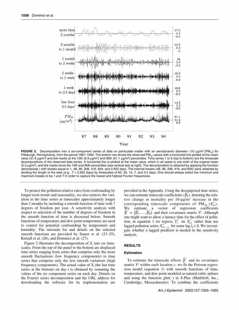
Figure 2 illustrates the decomposition of Xt into six time-scales. From the top of the panel to the bottom are displayedtime series ranging from series that comprise only the moresmooth fluctuations (low frequency components) to timeseries that comprise only the less smooth variations (highfrequency components). The actual value of Xt (the last timeseries at the bottom) on day t is obtained by summing thevalues of the six component series on each day. Details onthe Fourier series decomposition and the URL address fordownloading the software for its implementation are

provided in the Appendix. Using the decomposed time series,we can estimate timescale coefficients denoting the rela-tive change in mortality per 10-µg/m3 increase in thecorresponding timescale components of .We estimate a vector of regression coefficients

and their covariance matrix Vc. Althoughone might want to allow a latency time for the effect of pollu-tion, in equation 1 we regress on rather than uselagged pollution series for some lag lk > 0. We investi-gate whether a lagged predictor is needed in the sensitivityanalysis.

RESULTS

Estimation

To estimate the timescale effects and its covariancematrix Vc within each location c, we fit the Poisson regres-sion model (equation 1) with smooth functions of time,temperature, and dew point modeled as natural cubic splinesand using the function glm( ) in S-Plus (MathSoft, Inc.,Cambridge, Massachusetts). To combine the coefficients

FIGURE 2. Decomposition into a six-component series of data on particulate matter with an aerodynamic diameter ≤10 µg/m3 (PM10) forPittsburgh, Pennsylvania, from the period 1987–1994. The bottom row shows the observed PM10 values with a horizontal line plotted at the meanvalue (31.6 µg/m3) and tick marks at the 10th (8.9 µg/m3) and 90th (61.1 µg/m3) percentiles. Time series 1 to 6 (top to bottom) are the timescaledecompositions of the observed data series. A horizontal line is plotted at the mean value, which in all cases is one sixth of the original mean(5.3 µg/m3), and tick marks show the 10th and 90th percentiles (see vertical axis at right). The decomposition is obtained by applying the functiondecompose( ) with breaks equal to 1, 48, 96, 208, 416, 834, and 2,922 days. The internal breaks (48, 96, 208, 416, and 834) were obtained bydividing the length of the data (e.g., T = 2,922 days) by timescales of 60, 30, 14, 7, and 3.5 days. One should always select the minimum andmaximum breaks to be 1 and T in order to capture the lowest and highest Fourier frequencies.

β̂kc

( )

PM10 Xktc( )

β̂c β̂1c … β̂K

c,[ , ]=

Ytc

Xktc

Xkt lk–c

β̂c

Timescale Estimates of Particulate Matter Mortality Effects 1059

Am J Epidemiol 2003;157:1055–1065

across cities, we use a fixed-effect model with weights Wc =(Vc)–1 and an estimator of the form

with variance

.

An alternative approach would be to use as weights Wc =(D + Vc)–1, where D is a diagonal between-city covariance

matrix with diagonal element τ2. Because of the limitednumber of cities in the present analysis, we cannot estimateτ2 reliably and have assumed τ = 0. A sensitivity analysis ofour results with respect to different values of τ2 obtainedfrom hierarchical analyses of data from 20 cities (27) and 88cities (28) is discussed below.

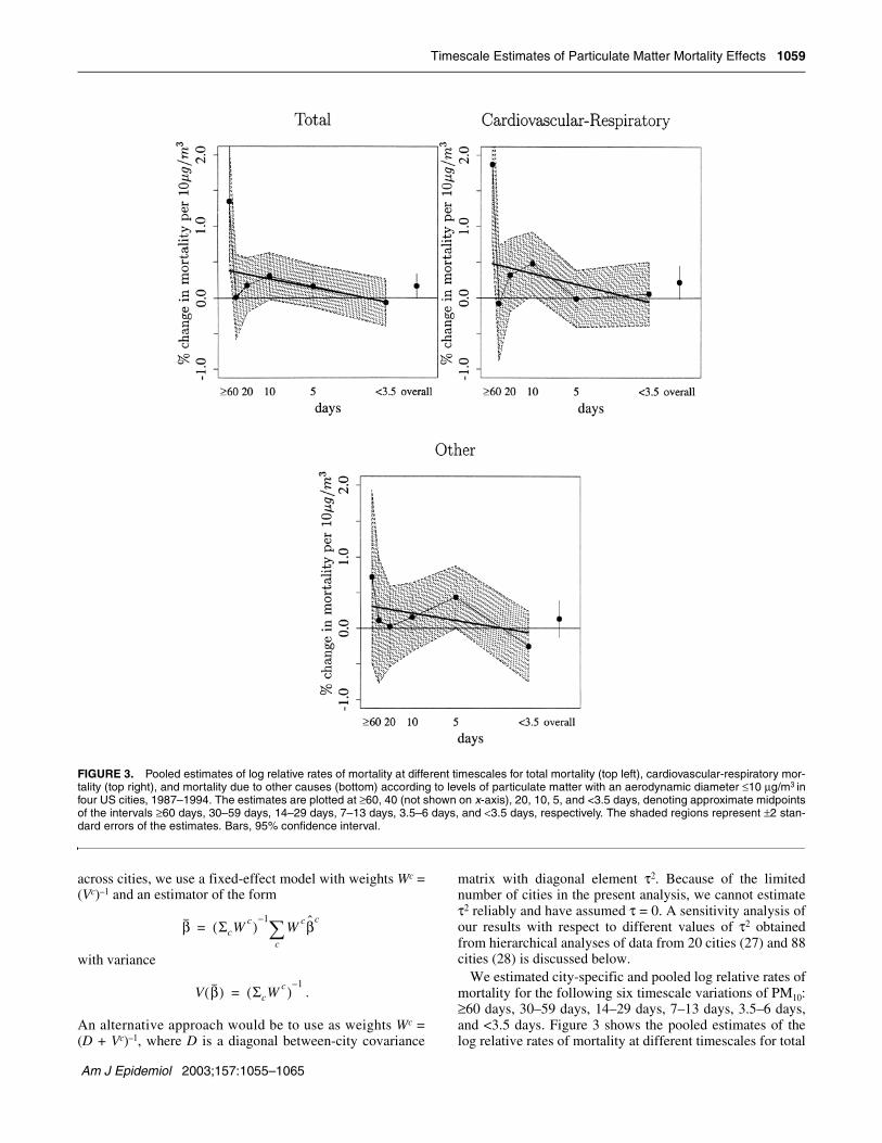
We estimated city-specific and pooled log relative rates ofmortality for the following six timescale variations of PM10:≥60 days, 30–59 days, 14–29 days, 7–13 days, 3.5–6 days,and <3.5 days. Figure 3 shows the pooled estimates of thelog relative rates of mortality at different timescales for total

β ΣcWc( )

1–W

c

c∑ β̂

c=

V β( ) ΣcW c( )1–

=

FIGURE 3. Pooled estimates of log relative rates of mortality at different timescales for total mortality (top left), cardiovascular-respiratory mor-tality (top right), and mortality due to other causes (bottom) according to levels of particulate matter with an aerodynamic diameter ≤10 µg/m3 infour US cities, 1987–1994. The estimates are plotted at ≥60, 40 (not shown on x-axis), 20, 10, 5, and <3.5 days, denoting approximate midpointsof the intervals ≥60 days, 30–59 days, 14–29 days, 7–13 days, 3.5–6 days, and <3.5 days, respectively. The shaded regions represent ±2 stan-dard errors of the estimates. Bars, 95% confidence interval.

1060 Dominici et al.

Am J Epidemiol 2003;157:1055–1065

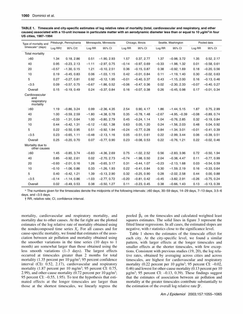
mortality, cardiovascular and respiratory mortality, andmortality due to other causes. At the far right are the plottedestimates of the log relative rate of mortality obtained usingthe nondecomposed time series Xt. For all causes and forcause-specific mortality, we found that estimates of the asso-ciation between air pollution and mortality obtained usingthe smoother variations in the time series (10 days to 1month) are somewhat larger than those obtained using theless smooth variations (1–3 days). The largest effectsoccurred at timescales greater than 2 months for totalmortality (1.35 percent per 10 µg/m3; 95 percent confidenceinterval (CI): 0.52, 2.17), cardiovascular and respiratorymortality (1.87 percent per 10 mg/m3; 95 percent CI: 0.75,2.99), and other-cause mortality (0.72 percent per 10 µg/m3;95 percent CI: –0.55, 1.95). To test the hypothesis that esti-mated effects at the longer timescales are larger thanthose at the shortest timescales, we linearly regress the

pooled on the timescales and calculated weighted leastsquares estimates. The solid lines in figure 3 represent thefitted linear regressions. In all cases, the estimated slopes arenegative, with t statistics close to the significance level.

Table 1 shows the estimates of the timescale effect foreach city. At the city-specific level, we found a similarpattern, with larger effects at the longer timescales andsmaller effects at the shorter timescales, with few excep-tions. Consistent with previous studies (19, 20), the log rela-tive rates, obtained by averaging across cities and acrosstimescales, are highest for cardiovascular and respiratorymortality (0.22 percent per 10 µg/m3; 95 percent CI: –0.02,0.46) and lowest for other-cause mortality (0.13 percent per 10µg/m3; 95 percent CI: –0.13, 0.39). These findings suggestthat the estimates of association between air pollution andmortality at the greater timescales contribute substantially tothe estimation of the overall log relative rate βc.

β̂k

TABLE 1. Timescale and city-specific estimates of log relative rates of mortality (total, cardiovascular and respiratory, and other causes) associated with a 10-unit increase in particulate matter with an aerodynamic diameter less than or equal to 10 µg/m3 in four US cities, 1987–1994

* The numbers given for the timescales denote the midpoints of the following intervals: ≥60 days, 30–59 days, 14–29 days, 7–13 days, 3.5–6days, and <3.5 days.

† RR, relative rate; CI, confidence interval.

Type of mortality and timescale* (days)

Pittsburgh, Pennsylvania Minneapolis, Minnesota Chicago, Illinois Seattle, Washington Pooled data

Log RR† 95% CI† Log RR 95% CI Log RR 95% CI Log RR 95% CI Log RR 95% CI

Total mortality

≥60 1.34 0.18, 2.86 0.51 –1.90, 2.93 1.57 0.37, 2.77 1.37 –0.98, 3.72 1.35 0.52, 2.17

40 0.95 –0.23, 2.13 –1.11 –2.97, 0.75 –0.14 –0.97, 0.69 –0.33 –1.98, 1.32 0.01 –0.58, 0.61

20 –0.57 –1.30, 0.15 1.21 –0.10, 2.51 0.36 –0.15, 0.87 0.38 –0.92, 1.69 0.18 –0.20, 0.56

10 0.19 –0.45, 0.83 0.06 –1.03, 1.15 0.42 –0.01, 0.84 0.11 –1.19, 1.40 0.30 –0.02, 0.63

5 0.27 –0.27, 0.81 0.92 –0.12, 1.95 –0.01 –0.40, 0.37 0.43 –1.15, 2.00 0.16 –0.13, 0.46

<3.5 0.09 –0.57, 0.75 –0.67 –1.86, 0.52 –0.06 –0.47, 0.36 0.02 –2.30, 2.33 –0.07 –0.40, 0.27

Overall 0.15 –0.19, 0.49 0.24 –0.37, 0.84 0.16 –0.07, 0.38 0.26 –0.45, 0.98 0.17 –0.01, 0.34

Cardiovascular and respiratory mortality

≥60 1.19 –0.86, 3.24 0.99 –2.36, 4.35 2.54 0.90, 4.17 1.86 –1.44, 5.15 1.87 0.75, 2.99

40 1.00 –0.59, 2.59 –1.80 –4.38, 0.78 0.35 –0.78, 1.48 –2.67 –4.95, –0.39 –0.08 –0.89, 0.74

20 –0.33 –1.31, 0.64 1.00 –0.80, 2.79 0.45 –0.24, 1.14 1.04 –0.76, 2.85 0.32 –0.19, 0.84

10 0.44 –0.42, 1.31 –0.12 –1.62, 1.38 0.63 0.05, 1.20 0.24 –1.56, 2.03 0.48 0.04, 0.92

5 0.22 –0.50, 0.95 0.51 –0.92, 1.94 –0.24 –0.77, 0.28 0.84 –1.34, 3.01 –0.01 –0.41, 0.39

<3.5 0.23 –0.65, 1.11 –0.48 –2.13, 1.16 0.05 –0.51, 0.61 0.22 –2.99, 3.44 0.06 –0.39, 0.51

Overall 0.25 –0.20, 0.70 0.07 –0.77, 0.90 0.23 –0.08, 0.53 0.22 –0.76, 1.21 0.22 –0.02, 0.46

Mortality due to other causes

≥60 1.45 –0.85, 3.74 –0.83 –4.36, 2.69 0.75 –1.02, 2.52 0.56 –2.83, 3.96 0.72 –0.50, 1.94

40 0.85 –0.92, 2.61 0.02 –2.70, 2.73 –0.74 –1.98, 0.50 2.04 –0.38, 4.47 0.11 –0.77, 0.99

20 –0.93 –2.01, 0.16 1.26 –0.65, 3.17 0.31 –0.44, 1.07 –0.23 –2.13, 1.68 0.03 –0.54, 0.59

10 –0.10 –1.06, 0.86 0.33 –1.26, 1.93 0.22 –0.41, 0.84 0.30 –1.59, 2.19 0.16 –0.33, 0.64

5 0.40 –0.42, 1.21 1.39 –0.13, 2.90 0.32 –0.25, 0.90 0.28 –2.02, 2.58 0.44 0.00, 0.88

<3.5 –0.14 –1.14, 0.86 –1.03 –2.77, 0.72 –0.20 –0.81, 0.42 –0.45 –3.82, 2.91 –0.26 –0.75, 0.24

Overall 0.02 –0.49, 0.53 0.38 –0.50, 1.27 0.11 –0.23, 0.45 0.38 –0.66, 1.43 0.13 –0.13, 0.39

Timescale Estimates of Particulate Matter Mortality Effects 1061

Am J Epidemiol 2003;157:1055–1065

Sensitivity analysis and model comparison

Below we investigate the sensitivity of our results withrespect to: 1) lag choice in the air pollution time series;2) adjustment for long-term trends and seasonality; and3) the degree of heterogeneity of the true relative ratesamong cities. We also apply our timescale approach to thePhiladelphia database for 1973–1988 that was previouslyanalyzed by Zeger et al. (10), to compare methods used herewith the frequency domain log-linear regression estimatespreviously published.

We first test the sensitivity of the log relative rate esti-mates to the choice of lag for component exposure series attimescales shorter than 1 month. We assume that the lag lk is0 for timescales greater than 1 month, since lags of 4 dayswill have little effect on the results for large timescales. Wefit several different lags for each component exposure series

and choose the best lag lk (the one with the largest tstatistic) rather than assume that lk is 0. The optimal lagswere obtained by including all timescale components in themodels; they are summarized in table 2. Results for totalmortality with an optimal lag compared with the originalmodel with a zero lag are shown in the upper half of figure 4.Although the estimates differ at particular timescales, theoverall shape of the curves remains similar and remainsinconsistent with the short-term mortality displacementhypothesis.

Our model controls for long-term trends in mortality byincluding a natural cubic spline of time with 7 degrees offreedom per year. To assess the sensitivity of the results tothe choice of smoothing parameter, we repeat the analysisusing 3.5 and 14 degrees of freedom per year. The lower halfof figure 4 shows the resulting plots. As expected, when lessflexible curves are used (fewer degrees of freedom), there isless control for trend and seasonality, and therefore theeffects at the longer timescales tend to be higher.

Our strategy for investigating the impact of the assumptionof homogeneity (τ = 0) of the pollution effects on our resultsis based on inspecting the pooled timescale estimates fortotal mortality under four alternative values for τ. Thesewere extracted from Bayesian hierarchical analyses of 20cities (27) and the 88 largest cities in the United States (28).The posterior mean values of τ and the corresponding priordistributions are summarized in table 3.

Results are shown in table 4. The results were all obtainedby using smooth functions (natural cubic splines) of timewith 7 degrees of freedom per year and smooth functions(natural cubic splines) of temperature and dew point as

Xkt l– k

TABLE 2. Analysis of the sensitivity of estimated log relative rates of mortality due to air pollution to the choice of lag for exposure series at timescales shorter than 1 month in four US cities, 1987–1994*

* The table summarizes, for each city and each timescale, the lagassociated with the largest t statistic.

City14–29 days

7–13 days

3.5–6 days

<3.5 days

Pittsburgh, Pennsylvania 1 2 0 6

Minneapolis, Minnesota 0 5 2 3

Chicago, Illinois 0 0 6 5

Seattle, Washington 0 3 6 4

FIGURE 4. Top: Sensitivity analysis showing stepwise pooled esti-mates for the total mortality and PM10 (particulate matter with anaerodynamic diameter ≤10 µg/m3) data series (four US cities, 1987–1994) and model 1 (see equation 1 in text). Bottom: Sensitivity anal-ysis showing pooled estimates for the total mortality and PM10 dataseries using different numbers of degrees of freedom (df) for time butthe same smooth function for temperature and humidity. The esti-mates are plotted at ≥60, 40 (not shown on x-axis), 20, 10, 5, and<3.5 days, denoting approximate midpoints of the intervals ≥60 days,30–59 days, 14–29 days, 7–13 days, 3.5–6 days, and <3.5 days,respectively. Bars, 95% confidence interval.

1062 Dominici et al.

Am J Epidemiol 2003;157:1055–1065

confounders, as in model 1 (equation 1). Although the confi-dence intervals widen considerably, the pooled estimates arenot very sensitive to the different values of τ. Even in thepresence of substantial heterogeneity of the relative rates ofmortality across cities, we still found that the pooled esti-mates at the longer timescales are larger than the pooled esti-mates at the shorter timescales, but with larger standarderrors.

We now apply timescale and frequency domain log-linearregression analyses (10, 15) to the Philadelphia data set, andwe estimate relative rates of mortality for exposure to airpollution at different timescales by using the Poisson regres-sion model defined in equation 1. Figure 5 shows thefrequency domain estimate of the mortality relative rateassociated with air pollution as a function of Fourierfrequency. Similar to the timescale result, the horizontal axesdenote the Fourier frequencies (lower x-axis) and the time-scale in days (upper x-axis) at which the association ismeasured. The solid curve and dotted curves denote the esti-mated relative rates ±2 estimated standard errors at eachfrequency. The timescale estimates (points connected by linesegments) are plotted on top of the frequency domain results(continuous curve). Timescale estimates and frequencydomain results are similar, and consistently with our resultsfor the four cities, relative rate estimates at longer timescalesare larger than relative rate estimates at short timescales.

DISCUSSION

This paper provides additional evidence that the associationbetween particle indexes and mortality is greater at longertimescales (10 days to 2 months) than at timescales of a fewdays. This suggests that the association of air pollution withdaily mortality counts does not reflect short-term mortalitydisplacement alone. More specifically, our results are incon-sistent with the “harvesting only” hypothesis, which contendsthat the air pollution-mortality association is caused entirelyby frail persons’ dying a few days earlier than they would haveabsent pollution. Under that hypothesis, we would anticipatelittle or no association at longer timescales. In fact, we observethe strongest associations there.

The larger relative rates at longer timescales may partlyreflect a greater biologic impact on chronic exposures thanon acute exposures. In fact, estimated relative risks from theHarvard Six Cities (7) and American Cancer Society (8)cohort studies, which address chronic exposures, are largerthan estimates from times-series models (28), which areconstrained to estimate the effects of shorter-timescale expo-sures.

The estimated relative rate of total mortality for the longesttimescale (2 months) was 1.35 percent per 10-unit increasein PM10 for the four cities considered. While 1.35 percent isapproximately 8 times larger than the overall pooled esti-

TABLE 3. Sensitivity analysis of pooled estimates of the log relative rate of mortality due to air pollution with respect to the amount of heterogeneity (τ)*

* The table summarizes posterior mean values of τ used to calculate the pooledeffect.

† N denotes the normal distribution.‡ IG denotes the inverse gamma distribution.

E [τ|data] Prior distribution Published reference

0.15 τ2 ∼ N†(0, 305) 20-city analysis (discussion and rejoinder of Dominici et al. (27))

0.38 τ2 ∼ N(0, 1) 88-city analysis (Dominici et al. (28))

0.49 τ2 ∼ IG‡(3, 1) 88-city analysis (Dominici et al. (28))

0.76 τ2 ∼ IG(3, 6) 20-city analysis (Dominici et al. (27))

Iτ2 0>

Iτ2 0>

TABLE 4. Pooled estimates of the log relative rate of mortality due to air pollution under different values of the heterogeneity parameter τ

* The numbers given for the timescale denote the midpoints of the following intervals: ≥60 days, 30–59 days, 14–29 days, 7–13 days, 3.5–6days, and <3.5 days.

† RR, relative rate; CI, confidence interval.

Timescale* (days)

τ = 0 τ = 0.15 τ = 0.38 τ = 0.49 τ = 0.76

Log RR† 95% CI† Log RR 95% CI Log RR 95% CI Log RR 95% CI Log RR 95% CI

≥60 1.35 0.52, 2.17 1.34 0.50, 2.18 1.32 0.39, 2.25 1.31 0.32, 2.30 1.29 0.12, 2.45

40 0.01 –0.58, 0.61 0.01 –0.61, 0.63 0.00 –0.74, 0.73 –0.02 –0.83, 0.79 –0.05 –1.06, 0.96

20 0.18 –0.20, 0.56 0.18 –0.24, 0.60 0.21 –0.36, 0.79 0.24 –0.43, 0.90 0.28 –0.61, 1.18

10 0.30 –0.02, 0.63 0.28 –0.09, 0.66 0.24 –0.31, 0.79 0.23 –0.41, 0.87 0.21 –0.66, 1.09

5 0.16 –0.13, 0.46 0.20 –0.15, 0.55 0.29 –0.25, 0.83 0.32 –0.32, 0.95 0.36 –0.52, 1.23

<3.5 –0.07 –0.40, 0.34 –0.07 –0.46, 0.32 –0.11 –0.69, 0.47 –0.12 –0.80, 0.56 –0.14 –1.07, 0.78

Overall 0.17 –0.01, 0.34 0.18 –0.07, 0.43 0.19 –0.26, 0.64 0.19 –0.35, 0.74 0.20 –0.60, 1.00

Timescale Estimates of Particulate Matter Mortality Effects 1063

Am J Epidemiol 2003;157:1055–1065

mate of 0.17 percent, it is still an order of magnitude smallerthan the estimated relative risks from the cohort studies (7,8). Thus, the time-series relative rates, even when restrictedto longer-term exposures, are much smaller than those fromthe major cohort studies. This difference might indicate thatthe most harmful exposures occur over much larger time-scales than can be studied with time-series methods.However, relative rate estimates at the longer timescalesshould be interpreted with caution because of theconfounding effects of seasonality and trend.

Our results are consistent with findings from previousreports for Philadelphia (10), Boston (11), and Chicago (12)that have used harvesting-resistant estimators. Thesemethods are based on a conceptually straightforward stratifi-cation of the air pollution time series into different frequencybands, allowing assessment of associations on timescaleswith differing implications.

Our approach and the approaches proposed by Zeger et al.(10) and Schwartz (11, 12) address related but different ques-tions. Zeger et al. (10) and Schwartz (11, 12) decompose boththe air pollution time series and the mortality time series intodifferent timescales of variation (Xkt and Ykt) and then aim toidentify the timescale component that leads to the strongestassociation between time-averaged air pollution and time-averaged mortality. The timescale analysis proposed in thispaper decomposes only the air pollution time series intodifferent timescales (Xkt) and then characterizes the timescalevariation of the effect of exposure on daily mortality. Forlinear models, these two approaches will provide the same

results. In Poisson regression, with small effects such as thosethat occur with air pollution variables, the differences betweenresults from the two approaches will probably be small. Ourapproach, however, is applicable over the range of Poisson orother generalized linear model applications.

The timescale decomposition shown in figure 2 could havebeen performed using wavelet methods. Wavelets are anatural extension of Fourier analysis; however, in waveletanalysis, the window or “scale” with which we look at theinformation stream is selected automatically. In our context,this automatic selection of the timescales is not particularlydesirable. One of the advantages of using wavelets is thatfunctions with discontinuities and functions with sharpspikes can be represented using substantially fewer waveletbasis elements than sine-cosine basis elements. Because acommon characteristic of time series of mortality, air pollu-tion, and weather data is their periodicity without largediscontinuities, Fourier analysis is adequate for our purpose.

The mortality displacement problem that motivated thedevelopment of this method is not unique to air pollution; ithas also been discussed in relation to heat waves and influ-enza. The statistical approach proposed in this paper is suit-able for these or other epidemiologic analyses with the focusof differentiating short-term effects from long-term effectsof a time-varying exposure on a health outcome. The set oftimescales selected should match hypotheses concerningrelations between exposure time and response. We alsoprovide an alternative strategy with which to control for

FIGURE 5. Change in mortality according to level of total suspended particulates (TSP) (particulate matter with an aerodynamic diameter ≤10 µg/m3) in Philadelphia, Pennsylvania, 1973–1988. The figure depicts a comparison between frequency domain estimates (continuous curve) and time-scale estimates (points connected by line segments), showing the log relative rates of total mortality by frequency and frequency grouping. Thedotted lines show ±2 standard errors for the frequency domain estimates, and the bars represent ±2 standard errors for the timescale estimates.

1064 Dominici et al.

Am J Epidemiol 2003;157:1055–1065

temporal confounding, since it is likely that confoundingmay vary with the timescale.

The timescale estimates from model 1 lead to specificpatterns for the coefficients of a distributed lag model (9, 29,30). A large effect at timescale k corresponds to an increasednumber of deaths for k/2 days after an air pollution episode,followed by a rebound below the baseline level for another k/2days, owing to the depletion of the pool of susceptible people.

Unlike the distributed lag model, our approach issymmetric in time; that is, we use a symmetric time window(t – lk, t + lk) to estimate Xkt. The temporal symmetry of ourapproach does not complicate our inferences, for tworeasons. First, and most importantly, it is not plausible thatmortality causes air pollution; it is only reasonable toconsider the possibility that air pollution causes mortality.Second, we use a symmetric time window simply to betterestimate the smooth variations of air pollution Xkt.

Other key methodological issues in time-series studies ofair pollution and mortality are the nonlinearity in the dose-response curves, the effect of copollutants, and the effect ofmeasurement error. These issues are discussed elsewhereand remain a topic of investigation (25, 28, 31, 32). In thecontext of mismeasurement of exposure, it is expected thatthe relative rate of mortality corresponding to the short timescales might be more attenuated by the measurement errorthan the relative rate of mortality corresponding to longertimescales. This is because more of the short timescale signalis actually error, whereas the longer timescale measure haseffectively been smoothed so that measurement error is lessof a contributor and hence less a source of bias. However,measurement error will not reverse the sign of an estimatedcoefficient or reverse the shape of the curve in figure 3.Therefore, even in the presence of measurement error, ourresults still do not support the “harvesting hypothesis” thatthe association between particle concentrations andmortality is entirely due to mortality among very frailpersons who lose a few days of life.

ACKNOWLEDGMENTS

The research described in this article was conductedunder contract with the Health Effects Institute, an organi-zation jointly funded by the Environmental ProtectionAgency (grant EPA R824835) and automotive manufac-turers. The contents of this article do not necessarily reflectthe views and policies of the Health Effects Institute, theEnvironmental Protection Agency, or motor vehicle orengine manufacturers. Funding for Dr. Francesca Dominiciwas provided by the Health Effects Institute (Walter A.Rosenblith New Investigator Award) and the ToxicSubstances Research Initiative of Health Canada. Thisresearch was also supported by a grant from the NationalInstitute of Environmental Health Sciences to the JohnsHopkins Center in Urban Environmental Health (grant P30ES0 3819-12).

The authors thank Drs. Rafael Irizarry, GiovanniParmigiani, and Marina Vannucci for comments on anearlier draft of the paper.

REFERENCES

1. Committee of the Environmental and Occupational HealthAssembly of the American Thoracic Society. Health effects ofoutdoor air pollution. [Part 1]. Am J Respir Crit Care Med1996;153:3–50.

2. Committee of the Environmental and Occupational HealthAssembly of the American Thoracic Society. Health effects ofoutdoor air pollution. Part 2. Am J Respir Crit Care Med 1996;153:477–98.

3. Pope CA III, Dockery DW, Schwartz J. Review of epidemio-logical evidence of health effects of particulate air pollution.Inhal Toxicol 1995;7:1–18.

4. Environmental Protection Agency, Office of Air Quality Plan-ning and Standards. Review of the National Ambient Air Qual-ity Standards for Particulate Matter: policy assessment ofscientific and technical information. OAQPS Staff Paper.Research Triangle Park, NC: Environmental ProtectionAgency, 1996. (Publication no. EPA-452\R-96-013).

5. Schimmel H, Murawski TJ. Proceedings: the relation of air pol-lution to mortality. J Occup Med 1976;18:316–33.

6. Lipfert FW, Wyzga RE. Air pollution and mortality: issues anduncertainties. J Air Waste Manage Assoc 1995;45:949–66.

7. Dockery DW, Pope CA III, Xu X, et al. An association betweenair pollution and mortality in six U.S. cities. N Engl J Med1993;329:1753–9.

8. Pope CA III, Thun MJ, Namboordiri MM, et al. Particulate airpollution as a predictor of mortality in a prospective study ofU.S. adults. Am J Respir Crit Care Med 1995;151:669–74.

9. Zanobetti A, Schwartz J, Samoli E, et al. The temporal patternof mortality responses to air pollution: a multicity assessmentof mortality displacement. Epidemiology 2002;13:87–93.

10. Zeger SL, Dominici F, Samet J. Harvesting-resistant estimatesof air pollution effects on mortality. Epidemiology 1999;10:171–5.

11. Schwartz J. Harvesting and long term exposure effects in therelationship between air pollution and mortality. Am J Epide-miol 2000;151:440–8.

12. Schwartz J. Is there harvesting in the association of airborneparticles with daily deaths and hospital admissions?Epidemiology 2001;12:55–61.

13. Spix C, Heinrich J, Dockery D, et al. Air pollution and dailymortality in Erfurt, East Germany, 1980–1989. Environ HealthPerspect 1993;101:518–26.

14. Smith RL, Davis JM, Speckman P. Human health effects ofenvironmental pollution in the atmosphere. In: Barnett V, SteinA, Turkman F, eds. Statistics in the environment 4: statisticalaspects of health and the environment. Chichester, UnitedKingdom: John Wiley and Sons Ltd, 1999:91–115.

15. Kelsall J, Zeger S, Samet J. Frequency domain log-linear mod-els: air pollution and mortality. Appl Stat 1999;48:331–44.

16. Cleveland WS, Develin SJ. Robust locally-weighted regressionand smoothing scatterplots. J Am Stat Assoc 1988;74:829–36.

17. Bloomfield P. Fourier analysis of time series: an introduction.New York, NY: John Wiley and Sons, Inc, 1976.

18. Priestley MB. Spectral analysis and time series. New York,NY: Academic Press, Inc, 1981.

19. Samet JM, Zeger SL, Dominici F, et al. The National Morbid-ity, Mortality, and Air Pollution Study. Part II: morbidity and

Timescale Estimates of Particulate Matter Mortality Effects 1065

Am J Epidemiol 2003;157:1055–1065

mortality from air pollution in the United States. Cambridge,MA: Health Effects Institute, 2000.

20. Samet JM, Dominici F, Zeger SL, et al. The National Morbid-ity, Mortality, and Air Pollution Study. Part I: methods andmethodologic issues. Cambridge, MA: Health Effects Institute,2000.

21. EarthInfo, Inc. NCDC Surface Airways. Boulder, CO: Earth-Info, Inc, 1994. (World Wide Web URL: http://www.earth-info.com/databases/sa.htm).

22. Environmental Protection Agency. Aerometric InformationRetrieval System. Washington, DC: Environmental ProtectionAgency, 1999. (World Wide Web URL: http://www.epa.gov/air/data/info.html).

23. Samet JM, Zeger SL, Berhane K. The association of mortalityand particulate air pollution. Part I. Particulate air pollution anddaily mortality: replication and validation of selected studies.Cambridge, MA: Health Effects Institute, 1995:1–104.

24. Samet JM, Zeger SL, Kelsall JE, et al. Particulate air pollutionand daily mortality: analyses of the effects of weather and mul-tiple air pollutants. The phase IB report of the Particle Epidemi-ology Evaluation Project. Cambridge, MA: Health EffectsInstitute, 1997.

25. Samet JM, Dominici F, Curriero FC, et al. Fine particulate airpollution and mortality in 20 U.S. cities, 1987–1994. N Engl JMed 2000;343:1742–9.

26. Kelsall JE, Samet JM, Zeger SL, et al. Air pollution and mortal-ity in Philadelphia, 1974–1988. Am J Epidemiol 1997;146:750–62.

27. Dominici F, Samet J, Zeger SL. Combining evidence on air pol-lution and daily mortality from the largest 20 U.S. cities: a hier-archical modeling strategy (with discussion). J R Stat Soc Ser A2000;163:263–302.

28. Dominici F, Daniels M, Zeger SL, et al. Air pollution and mor-tality: estimating regional and national dose-response relation-ships. J Am Stat Assoc 2002;97:100–11.

29. Almon S. The distributed lag between capital appropriationsand expenditures. Econometrica 1965;33:178–96.

30. Zanobetti A, Wand M, Schwartz J. Generalized additive dis-tributed lag models. Biostatistics 2000;1:279–92.

31. Daniels MJ, Dominici F, Samet JM, et al. Estimating particu-late matter-mortality dose-response curves and threshold lev-els: an analysis of daily time-series for the 20 largest US cities.Am J Epidemiol 2000;152:397–406.

32. Dominici F, Zeger S, Samet J. A measurement error correctionmodel for time-series studies of air pollution and mortality.Biostatistics 2000;1:157–74.

APPENDIX

Here we outline the approach to decomposing a daily timeseries Xt into timescale components {Xkt :

through the use of the discrete Fourier transform. Thediscrete Fourier transform is defined as

where T is the length of the series Xt and ωj = 2πj/T is the jthFourier frequency with j cycles in the length of the data.Note that if j = 1, then ω1 = 2π/T is a Fourier frequency withone cycle in the length of the data and describes the longest-term fluctuations. We note that when j ≥ T/2, we haved(ωT – j) = , where denotes the complex conju-gate of d(ωj). If T is even and j = T/2, then ωT/2 = π is aFourier frequency with a cycle for 2 days and describes theshortest-term fluctuations. Similarly, if T is odd and j = (T –1)/2, then

is the Fourier frequency describing the shortest-term fluctu-ations.

Let [0, ω1, …, ωk, …, ωK, π] be a partition of the interval[0, π], and we define Ik = (ωk–1, ωk] ∪ [ωT – k, ωT – k + 1). Thefollowing holds:

We can decompose the Xt into Xkt’s by implementing thefollowing algorithm. For k = 1, …, K:

• Taper the data Xt and get • Calculate the discrete Fourier transform of and get

d(ωj).

• Set

• Get Xkt by applying the inverse of the discrete Fouriertransform to d*(ωj), j = 1, …, T/2.

SAS, S-Plus, and R software for decomposing a timeseries into a desired set of frequency components can bedownloaded at http://www.ihapss.jhsph.edu/software/fd/software_fd.htm.Σk 1=

K Xkt Xt= }

d ωj( ) 1T--- Xtexp i– ωjt( ),

t 0=

T 1–

∑=

0 j T 1, 0 ωj 2≤ ≤ π,–≤ ≤

d ωj( ) d ωj( )

ωT 1– 2⁄T 1–

T------------π=

Xt Σj 0=T 1–

d ωj( )exp iωjt( )=

Σk 0=K Σωj Ik∈ d ωj( )exp iωjt( )[ ]=

Σk 0=K

Xkt.=

Xt.Xt

d∗ ωj( ) d ωj( ) for ωj Ik∈0 otherwise.

=

1055 Am J Epidemiol 2003;157:1055–1065

Volume 157

Number 12

June 15, 2003

American Journal of

EPIDEMIOLOGYCopyright © 2003 by The Johns Hopkins

Bloomberg School of Public Health

Sponsored by the Society for Epidemiologic Research

Published by Oxford University Press

ORIGINAL CONTRIBUTIONS

Airborne Particulate Matter and Mortality: Timescale Effects in Four US Cities

Francesca Dominici1, Aidan McDermott1, Scott L. Zeger1, and Jonathan M. Samet2

1 Department of Biostatistics, Bloomberg School of Public Health, Johns Hopkins University, Baltimore, MD. 2 Department of Epidemiology, Bloomberg School of Public Health, Johns Hopkins University, Baltimore, MD.

Received for publication February 5, 2001; accepted for publication October 12, 2001.

While time-series studies have consistently provided evidence for an effect of particulate air pollution onmortality, uncertainty remains as to the extent of the life-shortening implied by those associations. In this paper,the authors estimate the association between air pollution and mortality using different timescales of variation inthe air pollution time series to gain further insight into this question. The authors’ method is based on a Fourierdecomposition of air pollution time series into a set of independent exposure variables, each representing adifferent timescale. The authors then use this set of variables as predictors in a Poisson regression model toestimate a separate relative rate of mortality for each exposure timescale. The method is applied to a databasecontaining information on daily mortality, particulate air pollution, and weather in four US cities (Pittsburgh,Pennsylvania; Minneapolis, Minnesota; Seattle, Washington; and Chicago, Illinois) from the period 1987–1994.The authors found larger relative rates of mortality associated with particulate air pollution at longer timescalevariations (14 days–2 months) than at shorter timescales (1–4 days). These analyses provide additional evidencethat associations between particle indexes and mortality do not imply only an advance in the timing of death bya few days for frail individuals.

air pollution; Fourier analysis; hierarchical model; mortality; Poisson distribution; time factors; time series

Abbreviations: CI, confidence interval; PM10, particulate matter with an aerodynamic diameter ≤10 µg/m3.

Editor’s note: An invited commentary on this articleappears on page 1066, and the authors’ response appears onpage 1071.

A number of studies over the last decade have shown anassociation between particle concentrations in outdoor airand daily mortality counts in urban locations (1–3). Theseassociations have been estimated through the use of Poissonregression methods, and the findings have been reported as

log relative rates of mortality associated with air pollutionlevels on recent days. These associations have been widelyinterpreted as reflecting the effect of air pollution on personswho have heightened susceptibility because of chronic heartor lung diseases (4).

Thus, the increased mortality associated with higher pollu-tion levels may be restricted to very frail people whose lifeexpectancy would have been short even without air pollu-tion. This possibility is termed the “mortality displacement”

Correspondence to Dr. Francesca Dominici, Department of Biostatistics, Bloomberg School of Public Health, Johns Hopkins University, 615 North Wolfe Street, Baltimore, MD 21205 (e-mail: fdominic@jhsph.edu).

1056 Dominici et al.

Am J Epidemiol 2003;157:1055–1065

or “harvesting” hypothesis (5). If an effect is evident only atshort timescales, pollution-related deaths are advanced byonly a few days, and in fact, the days of life lost might argu-ably be of low quality for the frail individuals at risk ofdying. Consequently, the public health relevance of the find-ings of the daily time-series studies has been questioned (6).The mortality displacement hypothesis received specificdiscussion in the 1996 Staff Paper on Particulate Matterprepared by the US Environmental Protection Agencybecause of its policy implications (4). The findings of twolong-term prospective cohort studies of air pollution andmortality, the Harvard Six Cities Study (7) and the AmericanCancer Society’s Cancer Prevention Study II (8), wereconsidered to offer critical evidence counter to the mortalitydisplacement hypothesis.

Several investigators have approached the problem ofmortality displacement using analytical models for dailytime-series data (9–12). If the association between air pollu-tion and mortality does reflect the existence of a pool of frailindividuals in the population, episodes of high pollution thatlead to increased mortality might reduce the size of this pool,and days subsequent to high-pollution days would then beexpected to show a reduced effect of air pollution. Therefore,the occurrence of this phenomenon can be investigated byassessing interaction between prior high-pollution days andthe effects of subsequent pollution exposure on mortalitycounts; under the mortality displacement hypothesis, a nega-tive interaction is predicted (13, 14).

Recently, Kelsall et al. (15) and Schwartz (11) developedrelated methods for analysis of daily time-series data, bothoffering approaches to estimating air pollution-mortalityassociations at varying timescales. More specifically, Kelsallet al.’s methodology gives a continuous smooth estimate ofrelative risk as a function of timescale (frequency domainlog-linear regression). Zeger et al. (10) applied the frequencydomain log-linear regression to previously analyzed data forPhiladelphia, Pennsylvania, from 1973–1988. Schwartz (11,12) used a filtering algorithm (16) to separate the timeseries of daily deaths, air pollution, and weather into long-wavelength components, midscale components, and residual,very short-term components and applied this method to dataon Boston, Massachusetts, from 1979–1986 and Chicago,Illinois, from 1988–1993. Note that both of these methods(10, 11) analyze both pollution and mortality on the sametimescales, i.e., shorter-term to longer-term. Both sets ofanalyses found effects on longer timescales.

In this paper, we extend the work by Zeger et al. (10) andSchwartz (11) in the methodological, substantive, and compu-tational arenas. More specifically, we develop a timescaledecomposition of a time series based on the discrete Fouriertransform; we introduce a two-stage model for combiningevidence across locations for estimation of pooled timescale-specific air pollution effects on mortality; and we provide thesoftware for decomposing a time series into a set of desiredtimescale components. At the first stage of the model, we useFourier series analyses (17, 18) to decompose the daily timeseries of the air pollution variable into distinct timescalecomponents. This decomposition leads to a set of orthogonalpredictors, each representing a specific timescale of variationin the exposure. We then use this set of predictors in Poisson

regression models to estimate a relative rate of mortality corre-sponding to each timescale exposure while controlling forother covariates such as temperature. A comparison betweenour approach and the frequency domain log-linear regressionanalysis is provided below in the section “Sensitivity analysisand model comparison.”

The method is applied to concentrations of particulatematter, based on measurements of particles with an aero-dynamic diameter less than or equal to 10 µg/m3 (PM10) anddaily mortality counts from four US cities—Pittsburgh,Pennsylvania; Minneapolis, Minnesota; Chicago, Illinois;and Seattle, Washington. These were four cities with dailyPM10 measurements that were among the 90 largest US citiesused in the National Morbidity, Mortality, and Air PollutionStudy (19, 20). The analyses are restricted to these citiesbecause they are the only US locations with daily air pollu-tion concentrations available in this database for this timeinterval, while in most other locations, PM10 levels weremeasured only every 6 days as required by the Environ-mental Protection Agency. Our approach is not suitable forevery-sixth-day PM10 data, for two reasons: 1) no informa-tion is available from the data for estimation of the short-term effects of air pollution on mortality and 2) because ofthe “aliasing” phenomenon, the effects of air pollution at thelonger timescales are distorted. In our context, the aliasingphenomenon occurs when the sampling interval is largerthan 1 day, so that variations in the daily time series at theshortest timescales produce an apparent effect at the longertimescales.

MATERIALS AND METHODS

Data

We used daily time series of mortality, weather, and airpollution data for Pittsburgh, Minneapolis, Chicago, andSeattle for the period 1987–1994 (see figure 1). Dailymortality counts were obtained from the National Center forHealth Statistics and were grouped by age (<65, 65–75, and>75 years) and by cause of death according to the Interna-tional Classification of Diseases, Ninth Revision (cardiovas-cular-respiratory mortality (cardiac conditions, codes 390–448; respiratory conditions, codes 490–496; influenza, code487; and pneumonia, codes 480–486, 507) and mortality dueto other remaining diseases). Accidental deaths wereexcluded. Hourly temperature and dew point data wereavailable from the National Climatic Data Center, assembledin a compact disk database from EarthInfo, Inc. (21). The airpollution data were obtained from the Aerometric Informa-tion Retrieval Service (22) database maintained by the Envi-ronmental Protection Agency. For the pollutants measuredon an hourly basis, we calculated the 24-hour average. Amore detailed description of the database has been publishedelsewhere (19, 20).

Methods

Below we describe our statistical approach to estimationof the association between air pollution and mortality usingdifferent timescales. We let be the air pollution timeXt

c

Timescale Estimates of Particulate Matter Mortality Effects 1057

Am J Epidemiol 2003;157:1055–1065

series and be the mortality time series in location c. Wefirst decompose the air pollution series into distinctcomponent series , one for each distinct timescale k, andthen we calculate the association between , withoutdecomposition, and each of the timescale components .The decomposition is obtained by applying the discreteFourier transform to the series (17, 18). Specifically, weassume

and

(1)

where ϕc denotes the overdispersion parameter and the ’s,the parameters of interest, denote the log relative rate ofdaily mortality for each 10-unit increase in the air pollutionlevel in location c on a timescale k. Our modeling approachreplaces the term , where is the air pollution timeseries and βc is the city-specific log relative rate of mortality,with the sum , where Xt = ΣkXkt, and the X1t, …, Xkt,…, XKt is a set of orthogonal predictors. This model estimatesrelative rates of mortality at different timescales and charac-terizes the timescale variation in the air pollution time seriesthat contributes to the estimate of the overall effect βc. Herewe expect that under a short-term mortality displacementscenario, mortality would be mainly associated with a short-term effect of air pollution.

FIGURE 1. Daily time series of mortality (total, cardiovascular disease (CVD) and respiratory (Resp), and other causes (Other)), temperature(Temp), and levels of particulate matter with an aerodynamic diameter less than 10 µg/m3 (PM10) for Pittsburgh, Pennsylvania, Minneapolis, Min-nesota, and Chicago, Illinois, during the period 1987–1994. For Seattle, Washington, data for the period 1989–1994 were used.

Ytc

Xtc

Xktc

Ytc

Xktc

Xtc

Ytc µt

c Poisson µtc( ) var Yt

c( );∼ ϕcµtc=

log µtc ΣkXkt

c βkc

S time 7 year⁄( , ) confounders,+ +=

βkc

Xtcβc

Xtc

ΣkXktc βk

c

1058 Dominici et al.

Am J Epidemiol 2003;157:1055–1065

To protect the pollution relative rates from confounding bylonger-term trends and seasonality, we also remove the vari-ation in the time series at timescales approximately longerthan 2 months by including a smooth function of time with 7degrees of freedom per year. A sensitivity analysis withrespect to selection of the number of degrees of freedom inthe smooth function of time is discussed below. Smoothfunctions of temperature and dew point temperature are usedto control for potential confounding by temperature andhumidity. The rationale for and details on the selectedsmooth functions are provided by Samet et al. (23–25),Kelsall et al. (26), and Dominici et al. (27).

Figure 2 illustrates the decomposition of Xt into six time-scales. From the top of the panel to the bottom are displayedtime series ranging from series that comprise only the moresmooth fluctuations (low frequency components) to timeseries that comprise only the less smooth variations (highfrequency components). The actual value of Xt (the last timeseries at the bottom) on day t is obtained by summing thevalues of the six component series on each day. Details onthe Fourier series decomposition and the URL address fordownloading the software for its implementation are

provided in the Appendix. Using the decomposed time series,we can estimate timescale coefficients denoting the rela-tive change in mortality per 10-µg/m3 increase in thecorresponding timescale components of .We estimate a vector of regression coefficients

and their covariance matrix Vc. Althoughone might want to allow a latency time for the effect of pollu-tion, in equation 1 we regress on rather than uselagged pollution series for some lag lk > 0. We investi-gate whether a lagged predictor is needed in the sensitivityanalysis.

RESULTS

Estimation

To estimate the timescale effects and its covariancematrix Vc within each location c, we fit the Poisson regres-sion model (equation 1) with smooth functions of time,temperature, and dew point modeled as natural cubic splinesand using the function glm( ) in S-Plus (MathSoft, Inc.,Cambridge, Massachusetts). To combine the coefficients

FIGURE 2. Decomposition into a six-component series of data on particulate matter with an aerodynamic diameter ≤10 µg/m3 (PM10) forPittsburgh, Pennsylvania, from the period 1987–1994. The bottom row shows the observed PM10 values with a horizontal line plotted at the meanvalue (31.6 µg/m3) and tick marks at the 10th (8.9 µg/m3) and 90th (61.1 µg/m3) percentiles. Time series 1 to 6 (top to bottom) are the timescaledecompositions of the observed data series. A horizontal line is plotted at the mean value, which in all cases is one sixth of the original mean(5.3 µg/m3), and tick marks show the 10th and 90th percentiles (see vertical axis at right). The decomposition is obtained by applying the functiondecompose( ) with breaks equal to 1, 48, 96, 208, 416, 834, and 2,922 days. The internal breaks (48, 96, 208, 416, and 834) were obtained bydividing the length of the data (e.g., T = 2,922 days) by timescales of 60, 30, 14, 7, and 3.5 days. One should always select the minimum andmaximum breaks to be 1 and T in order to capture the lowest and highest Fourier frequencies.

β̂kc

( )

PM10 Xktc( )

β̂c β̂1c … β̂K

c,[ , ]=

Ytc

Xktc

Xkt lk–c

β̂c

Timescale Estimates of Particulate Matter Mortality Effects 1059

Am J Epidemiol 2003;157:1055–1065

across cities, we use a fixed-effect model with weights Wc =(Vc)–1 and an estimator of the form

with variance

.

An alternative approach would be to use as weights Wc =(D + Vc)–1, where D is a diagonal between-city covariance

matrix with diagonal element τ2. Because of the limitednumber of cities in the present analysis, we cannot estimateτ2 reliably and have assumed τ = 0. A sensitivity analysis ofour results with respect to different values of τ2 obtainedfrom hierarchical analyses of data from 20 cities (27) and 88cities (28) is discussed below.

We estimated city-specific and pooled log relative rates ofmortality for the following six timescale variations of PM10:≥60 days, 30–59 days, 14–29 days, 7–13 days, 3.5–6 days,and <3.5 days. Figure 3 shows the pooled estimates of thelog relative rates of mortality at different timescales for total

β ΣcWc( )

1–W

c

c∑ β̂

c=

V β( ) ΣcW c( )1–

=

FIGURE 3. Pooled estimates of log relative rates of mortality at different timescales for total mortality (top left), cardiovascular-respiratory mor-tality (top right), and mortality due to other causes (bottom) according to levels of particulate matter with an aerodynamic diameter ≤10 µg/m3 infour US cities, 1987–1994. The estimates are plotted at ≥60, 40 (not shown on x-axis), 20, 10, 5, and <3.5 days, denoting approximate midpointsof the intervals ≥60 days, 30–59 days, 14–29 days, 7–13 days, 3.5–6 days, and <3.5 days, respectively. The shaded regions represent ±2 stan-dard errors of the estimates. Bars, 95% confidence interval.

1060 Dominici et al.

Am J Epidemiol 2003;157:1055–1065

mortality, cardiovascular and respiratory mortality, andmortality due to other causes. At the far right are the plottedestimates of the log relative rate of mortality obtained usingthe nondecomposed time series Xt. For all causes and forcause-specific mortality, we found that estimates of the asso-ciation between air pollution and mortality obtained usingthe smoother variations in the time series (10 days to 1month) are somewhat larger than those obtained using theless smooth variations (1–3 days). The largest effectsoccurred at timescales greater than 2 months for totalmortality (1.35 percent per 10 µg/m3; 95 percent confidenceinterval (CI): 0.52, 2.17), cardiovascular and respiratorymortality (1.87 percent per 10 mg/m3; 95 percent CI: 0.75,2.99), and other-cause mortality (0.72 percent per 10 µg/m3;95 percent CI: –0.55, 1.95). To test the hypothesis that esti-mated effects at the longer timescales are larger thanthose at the shortest timescales, we linearly regress the

pooled on the timescales and calculated weighted leastsquares estimates. The solid lines in figure 3 represent thefitted linear regressions. In all cases, the estimated slopes arenegative, with t statistics close to the significance level.

Table 1 shows the estimates of the timescale effect foreach city. At the city-specific level, we found a similarpattern, with larger effects at the longer timescales andsmaller effects at the shorter timescales, with few excep-tions. Consistent with previous studies (19, 20), the log rela-tive rates, obtained by averaging across cities and acrosstimescales, are highest for cardiovascular and respiratorymortality (0.22 percent per 10 µg/m3; 95 percent CI: –0.02,0.46) and lowest for other-cause mortality (0.13 percent per 10µg/m3; 95 percent CI: –0.13, 0.39). These findings suggestthat the estimates of association between air pollution andmortality at the greater timescales contribute substantially tothe estimation of the overall log relative rate βc.

β̂k

TABLE 1. Timescale and city-specific estimates of log relative rates of mortality (total, cardiovascular and respiratory, and other causes) associated with a 10-unit increase in particulate matter with an aerodynamic diameter less than or equal to 10 µg/m3 in four US cities, 1987–1994

* The numbers given for the timescales denote the midpoints of the following intervals: ≥60 days, 30–59 days, 14–29 days, 7–13 days, 3.5–6days, and <3.5 days.

† RR, relative rate; CI, confidence interval.

Type of mortality and timescale* (days)

Pittsburgh, Pennsylvania Minneapolis, Minnesota Chicago, Illinois Seattle, Washington Pooled data

Log RR† 95% CI† Log RR 95% CI Log RR 95% CI Log RR 95% CI Log RR 95% CI

Total mortality

≥60 1.34 0.18, 2.86 0.51 –1.90, 2.93 1.57 0.37, 2.77 1.37 –0.98, 3.72 1.35 0.52, 2.17

40 0.95 –0.23, 2.13 –1.11 –2.97, 0.75 –0.14 –0.97, 0.69 –0.33 –1.98, 1.32 0.01 –0.58, 0.61

20 –0.57 –1.30, 0.15 1.21 –0.10, 2.51 0.36 –0.15, 0.87 0.38 –0.92, 1.69 0.18 –0.20, 0.56

10 0.19 –0.45, 0.83 0.06 –1.03, 1.15 0.42 –0.01, 0.84 0.11 –1.19, 1.40 0.30 –0.02, 0.63

5 0.27 –0.27, 0.81 0.92 –0.12, 1.95 –0.01 –0.40, 0.37 0.43 –1.15, 2.00 0.16 –0.13, 0.46

<3.5 0.09 –0.57, 0.75 –0.67 –1.86, 0.52 –0.06 –0.47, 0.36 0.02 –2.30, 2.33 –0.07 –0.40, 0.27

Overall 0.15 –0.19, 0.49 0.24 –0.37, 0.84 0.16 –0.07, 0.38 0.26 –0.45, 0.98 0.17 –0.01, 0.34

Cardiovascular and respiratory mortality

≥60 1.19 –0.86, 3.24 0.99 –2.36, 4.35 2.54 0.90, 4.17 1.86 –1.44, 5.15 1.87 0.75, 2.99

40 1.00 –0.59, 2.59 –1.80 –4.38, 0.78 0.35 –0.78, 1.48 –2.67 –4.95, –0.39 –0.08 –0.89, 0.74

20 –0.33 –1.31, 0.64 1.00 –0.80, 2.79 0.45 –0.24, 1.14 1.04 –0.76, 2.85 0.32 –0.19, 0.84

10 0.44 –0.42, 1.31 –0.12 –1.62, 1.38 0.63 0.05, 1.20 0.24 –1.56, 2.03 0.48 0.04, 0.92

5 0.22 –0.50, 0.95 0.51 –0.92, 1.94 –0.24 –0.77, 0.28 0.84 –1.34, 3.01 –0.01 –0.41, 0.39

<3.5 0.23 –0.65, 1.11 –0.48 –2.13, 1.16 0.05 –0.51, 0.61 0.22 –2.99, 3.44 0.06 –0.39, 0.51

Overall 0.25 –0.20, 0.70 0.07 –0.77, 0.90 0.23 –0.08, 0.53 0.22 –0.76, 1.21 0.22 –0.02, 0.46

Mortality due to other causes

≥60 1.45 –0.85, 3.74 –0.83 –4.36, 2.69 0.75 –1.02, 2.52 0.56 –2.83, 3.96 0.72 –0.50, 1.94

40 0.85 –0.92, 2.61 0.02 –2.70, 2.73 –0.74 –1.98, 0.50 2.04 –0.38, 4.47 0.11 –0.77, 0.99

20 –0.93 –2.01, 0.16 1.26 –0.65, 3.17 0.31 –0.44, 1.07 –0.23 –2.13, 1.68 0.03 –0.54, 0.59

10 –0.10 –1.06, 0.86 0.33 –1.26, 1.93 0.22 –0.41, 0.84 0.30 –1.59, 2.19 0.16 –0.33, 0.64

5 0.40 –0.42, 1.21 1.39 –0.13, 2.90 0.32 –0.25, 0.90 0.28 –2.02, 2.58 0.44 0.00, 0.88

<3.5 –0.14 –1.14, 0.86 –1.03 –2.77, 0.72 –0.20 –0.81, 0.42 –0.45 –3.82, 2.91 –0.26 –0.75, 0.24

Overall 0.02 –0.49, 0.53 0.38 –0.50, 1.27 0.11 –0.23, 0.45 0.38 –0.66, 1.43 0.13 –0.13, 0.39

Timescale Estimates of Particulate Matter Mortality Effects 1061

Am J Epidemiol 2003;157:1055–1065

Sensitivity analysis and model comparison

Below we investigate the sensitivity of our results withrespect to: 1) lag choice in the air pollution time series;2) adjustment for long-term trends and seasonality; and3) the degree of heterogeneity of the true relative ratesamong cities. We also apply our timescale approach to thePhiladelphia database for 1973–1988 that was previouslyanalyzed by Zeger et al. (10), to compare methods used herewith the frequency domain log-linear regression estimatespreviously published.

We first test the sensitivity of the log relative rate esti-mates to the choice of lag for component exposure series attimescales shorter than 1 month. We assume that the lag lk is0 for timescales greater than 1 month, since lags of 4 dayswill have little effect on the results for large timescales. Wefit several different lags for each component exposure series

and choose the best lag lk (the one with the largest tstatistic) rather than assume that lk is 0. The optimal lagswere obtained by including all timescale components in themodels; they are summarized in table 2. Results for totalmortality with an optimal lag compared with the originalmodel with a zero lag are shown in the upper half of figure 4.Although the estimates differ at particular timescales, theoverall shape of the curves remains similar and remainsinconsistent with the short-term mortality displacementhypothesis.

Our model controls for long-term trends in mortality byincluding a natural cubic spline of time with 7 degrees offreedom per year. To assess the sensitivity of the results tothe choice of smoothing parameter, we repeat the analysisusing 3.5 and 14 degrees of freedom per year. The lower halfof figure 4 shows the resulting plots. As expected, when lessflexible curves are used (fewer degrees of freedom), there isless control for trend and seasonality, and therefore theeffects at the longer timescales tend to be higher.

Our strategy for investigating the impact of the assumptionof homogeneity (τ = 0) of the pollution effects on our resultsis based on inspecting the pooled timescale estimates fortotal mortality under four alternative values for τ. Thesewere extracted from Bayesian hierarchical analyses of 20cities (27) and the 88 largest cities in the United States (28).The posterior mean values of τ and the corresponding priordistributions are summarized in table 3.

Results are shown in table 4. The results were all obtainedby using smooth functions (natural cubic splines) of timewith 7 degrees of freedom per year and smooth functions(natural cubic splines) of temperature and dew point as

Xkt l– k

TABLE 2. Analysis of the sensitivity of estimated log relative rates of mortality due to air pollution to the choice of lag for exposure series at timescales shorter than 1 month in four US cities, 1987–1994*

* The table summarizes, for each city and each timescale, the lagassociated with the largest t statistic.

City14–29 days

7–13 days

3.5–6 days

<3.5 days

Pittsburgh, Pennsylvania 1 2 0 6

Minneapolis, Minnesota 0 5 2 3

Chicago, Illinois 0 0 6 5

Seattle, Washington 0 3 6 4

FIGURE 4. Top: Sensitivity analysis showing stepwise pooled esti-mates for the total mortality and PM10 (particulate matter with anaerodynamic diameter ≤10 µg/m3) data series (four US cities, 1987–1994) and model 1 (see equation 1 in text). Bottom: Sensitivity anal-ysis showing pooled estimates for the total mortality and PM10 dataseries using different numbers of degrees of freedom (df) for time butthe same smooth function for temperature and humidity. The esti-mates are plotted at ≥60, 40 (not shown on x-axis), 20, 10, 5, and<3.5 days, denoting approximate midpoints of the intervals ≥60 days,30–59 days, 14–29 days, 7–13 days, 3.5–6 days, and <3.5 days,respectively. Bars, 95% confidence interval.

1062 Dominici et al.

Am J Epidemiol 2003;157:1055–1065

confounders, as in model 1 (equation 1). Although the confi-dence intervals widen considerably, the pooled estimates arenot very sensitive to the different values of τ. Even in thepresence of substantial heterogeneity of the relative rates ofmortality across cities, we still found that the pooled esti-mates at the longer timescales are larger than the pooled esti-mates at the shorter timescales, but with larger standarderrors.

We now apply timescale and frequency domain log-linearregression analyses (10, 15) to the Philadelphia data set, andwe estimate relative rates of mortality for exposure to airpollution at different timescales by using the Poisson regres-sion model defined in equation 1. Figure 5 shows thefrequency domain estimate of the mortality relative rateassociated with air pollution as a function of Fourierfrequency. Similar to the timescale result, the horizontal axesdenote the Fourier frequencies (lower x-axis) and the time-scale in days (upper x-axis) at which the association ismeasured. The solid curve and dotted curves denote the esti-mated relative rates ±2 estimated standard errors at eachfrequency. The timescale estimates (points connected by linesegments) are plotted on top of the frequency domain results(continuous curve). Timescale estimates and frequencydomain results are similar, and consistently with our resultsfor the four cities, relative rate estimates at longer timescalesare larger than relative rate estimates at short timescales.

DISCUSSION

This paper provides additional evidence that the associationbetween particle indexes and mortality is greater at longertimescales (10 days to 2 months) than at timescales of a fewdays. This suggests that the association of air pollution withdaily mortality counts does not reflect short-term mortalitydisplacement alone. More specifically, our results are incon-sistent with the “harvesting only” hypothesis, which contendsthat the air pollution-mortality association is caused entirelyby frail persons’ dying a few days earlier than they would haveabsent pollution. Under that hypothesis, we would anticipatelittle or no association at longer timescales. In fact, we observethe strongest associations there.

The larger relative rates at longer timescales may partlyreflect a greater biologic impact on chronic exposures thanon acute exposures. In fact, estimated relative risks from theHarvard Six Cities (7) and American Cancer Society (8)cohort studies, which address chronic exposures, are largerthan estimates from times-series models (28), which areconstrained to estimate the effects of shorter-timescale expo-sures.

The estimated relative rate of total mortality for the longesttimescale (2 months) was 1.35 percent per 10-unit increasein PM10 for the four cities considered. While 1.35 percent isapproximately 8 times larger than the overall pooled esti-

TABLE 3. Sensitivity analysis of pooled estimates of the log relative rate of mortality due to air pollution with respect to the amount of heterogeneity (τ)*

* The table summarizes posterior mean values of τ used to calculate the pooledeffect.

† N denotes the normal distribution.‡ IG denotes the inverse gamma distribution.

E [τ|data] Prior distribution Published reference

0.15 τ2 ∼ N†(0, 305) 20-city analysis (discussion and rejoinder of Dominici et al. (27))

0.38 τ2 ∼ N(0, 1) 88-city analysis (Dominici et al. (28))

0.49 τ2 ∼ IG‡(3, 1) 88-city analysis (Dominici et al. (28))

0.76 τ2 ∼ IG(3, 6) 20-city analysis (Dominici et al. (27))

Iτ2 0>

Iτ2 0>

TABLE 4. Pooled estimates of the log relative rate of mortality due to air pollution under different values of the heterogeneity parameter τ

* The numbers given for the timescale denote the midpoints of the following intervals: ≥60 days, 30–59 days, 14–29 days, 7–13 days, 3.5–6days, and <3.5 days.

† RR, relative rate; CI, confidence interval.

Timescale* (days)

τ = 0 τ = 0.15 τ = 0.38 τ = 0.49 τ = 0.76

Log RR† 95% CI† Log RR 95% CI Log RR 95% CI Log RR 95% CI Log RR 95% CI

≥60 1.35 0.52, 2.17 1.34 0.50, 2.18 1.32 0.39, 2.25 1.31 0.32, 2.30 1.29 0.12, 2.45

40 0.01 –0.58, 0.61 0.01 –0.61, 0.63 0.00 –0.74, 0.73 –0.02 –0.83, 0.79 –0.05 –1.06, 0.96

20 0.18 –0.20, 0.56 0.18 –0.24, 0.60 0.21 –0.36, 0.79 0.24 –0.43, 0.90 0.28 –0.61, 1.18

10 0.30 –0.02, 0.63 0.28 –0.09, 0.66 0.24 –0.31, 0.79 0.23 –0.41, 0.87 0.21 –0.66, 1.09

5 0.16 –0.13, 0.46 0.20 –0.15, 0.55 0.29 –0.25, 0.83 0.32 –0.32, 0.95 0.36 –0.52, 1.23

<3.5 –0.07 –0.40, 0.34 –0.07 –0.46, 0.32 –0.11 –0.69, 0.47 –0.12 –0.80, 0.56 –0.14 –1.07, 0.78

Overall 0.17 –0.01, 0.34 0.18 –0.07, 0.43 0.19 –0.26, 0.64 0.19 –0.35, 0.74 0.20 –0.60, 1.00

Timescale Estimates of Particulate Matter Mortality Effects 1063

Am J Epidemiol 2003;157:1055–1065

mate of 0.17 percent, it is still an order of magnitude smallerthan the estimated relative risks from the cohort studies (7,8). Thus, the time-series relative rates, even when restrictedto longer-term exposures, are much smaller than those fromthe major cohort studies. This difference might indicate thatthe most harmful exposures occur over much larger time-scales than can be studied with time-series methods.However, relative rate estimates at the longer timescalesshould be interpreted with caution because of theconfounding effects of seasonality and trend.

Our results are consistent with findings from previousreports for Philadelphia (10), Boston (11), and Chicago (12)that have used harvesting-resistant estimators. Thesemethods are based on a conceptually straightforward stratifi-cation of the air pollution time series into different frequencybands, allowing assessment of associations on timescaleswith differing implications.

Our approach and the approaches proposed by Zeger et al.(10) and Schwartz (11, 12) address related but different ques-tions. Zeger et al. (10) and Schwartz (11, 12) decompose boththe air pollution time series and the mortality time series intodifferent timescales of variation (Xkt and Ykt) and then aim toidentify the timescale component that leads to the strongestassociation between time-averaged air pollution and time-averaged mortality. The timescale analysis proposed in thispaper decomposes only the air pollution time series intodifferent timescales (Xkt) and then characterizes the timescalevariation of the effect of exposure on daily mortality. Forlinear models, these two approaches will provide the same

results. In Poisson regression, with small effects such as thosethat occur with air pollution variables, the differences betweenresults from the two approaches will probably be small. Ourapproach, however, is applicable over the range of Poisson orother generalized linear model applications.

The timescale decomposition shown in figure 2 could havebeen performed using wavelet methods. Wavelets are anatural extension of Fourier analysis; however, in waveletanalysis, the window or “scale” with which we look at theinformation stream is selected automatically. In our context,this automatic selection of the timescales is not particularlydesirable. One of the advantages of using wavelets is thatfunctions with discontinuities and functions with sharpspikes can be represented using substantially fewer waveletbasis elements than sine-cosine basis elements. Because acommon characteristic of time series of mortality, air pollu-tion, and weather data is their periodicity without largediscontinuities, Fourier analysis is adequate for our purpose.

The mortality displacement problem that motivated thedevelopment of this method is not unique to air pollution; ithas also been discussed in relation to heat waves and influ-enza. The statistical approach proposed in this paper is suit-able for these or other epidemiologic analyses with the focusof differentiating short-term effects from long-term effectsof a time-varying exposure on a health outcome. The set oftimescales selected should match hypotheses concerningrelations between exposure time and response. We alsoprovide an alternative strategy with which to control for

FIGURE 5. Change in mortality according to level of total suspended particulates (TSP) (particulate matter with an aerodynamic diameter ≤10 µg/m3) in Philadelphia, Pennsylvania, 1973–1988. The figure depicts a comparison between frequency domain estimates (continuous curve) and time-scale estimates (points connected by line segments), showing the log relative rates of total mortality by frequency and frequency grouping. Thedotted lines show ±2 standard errors for the frequency domain estimates, and the bars represent ±2 standard errors for the timescale estimates.

1064 Dominici et al.

Am J Epidemiol 2003;157:1055–1065

temporal confounding, since it is likely that confoundingmay vary with the timescale.

The timescale estimates from model 1 lead to specificpatterns for the coefficients of a distributed lag model (9, 29,30). A large effect at timescale k corresponds to an increasednumber of deaths for k/2 days after an air pollution episode,followed by a rebound below the baseline level for another k/2days, owing to the depletion of the pool of susceptible people.

Unlike the distributed lag model, our approach issymmetric in time; that is, we use a symmetric time window(t – lk, t + lk) to estimate Xkt. The temporal symmetry of ourapproach does not complicate our inferences, for tworeasons. First, and most importantly, it is not plausible thatmortality causes air pollution; it is only reasonable toconsider the possibility that air pollution causes mortality.Second, we use a symmetric time window simply to betterestimate the smooth variations of air pollution Xkt.

Other key methodological issues in time-series studies ofair pollution and mortality are the nonlinearity in the dose-response curves, the effect of copollutants, and the effect ofmeasurement error. These issues are discussed elsewhereand remain a topic of investigation (25, 28, 31, 32). In thecontext of mismeasurement of exposure, it is expected thatthe relative rate of mortality corresponding to the short timescales might be more attenuated by the measurement errorthan the relative rate of mortality corresponding to longertimescales. This is because more of the short timescale signalis actually error, whereas the longer timescale measure haseffectively been smoothed so that measurement error is lessof a contributor and hence less a source of bias. However,measurement error will not reverse the sign of an estimatedcoefficient or reverse the shape of the curve in figure 3.Therefore, even in the presence of measurement error, ourresults still do not support the “harvesting hypothesis” thatthe association between particle concentrations andmortality is entirely due to mortality among very frailpersons who lose a few days of life.

ACKNOWLEDGMENTS

The research described in this article was conductedunder contract with the Health Effects Institute, an organi-zation jointly funded by the Environmental ProtectionAgency (grant EPA R824835) and automotive manufac-turers. The contents of this article do not necessarily reflectthe views and policies of the Health Effects Institute, theEnvironmental Protection Agency, or motor vehicle orengine manufacturers. Funding for Dr. Francesca Dominiciwas provided by the Health Effects Institute (Walter A.Rosenblith New Investigator Award) and the ToxicSubstances Research Initiative of Health Canada. Thisresearch was also supported by a grant from the NationalInstitute of Environmental Health Sciences to the JohnsHopkins Center in Urban Environmental Health (grant P30ES0 3819-12).

The authors thank Drs. Rafael Irizarry, GiovanniParmigiani, and Marina Vannucci for comments on anearlier draft of the paper.

REFERENCES

1. Committee of the Environmental and Occupational HealthAssembly of the American Thoracic Society. Health effects ofoutdoor air pollution. [Part 1]. Am J Respir Crit Care Med1996;153:3–50.

2. Committee of the Environmental and Occupational HealthAssembly of the American Thoracic Society. Health effects ofoutdoor air pollution. Part 2. Am J Respir Crit Care Med 1996;153:477–98.

3. Pope CA III, Dockery DW, Schwartz J. Review of epidemio-logical evidence of health effects of particulate air pollution.Inhal Toxicol 1995;7:1–18.

4. Environmental Protection Agency, Office of Air Quality Plan-ning and Standards. Review of the National Ambient Air Qual-ity Standards for Particulate Matter: policy assessment ofscientific and technical information. OAQPS Staff Paper.Research Triangle Park, NC: Environmental ProtectionAgency, 1996. (Publication no. EPA-452\R-96-013).

5. Schimmel H, Murawski TJ. Proceedings: the relation of air pol-lution to mortality. J Occup Med 1976;18:316–33.

6. Lipfert FW, Wyzga RE. Air pollution and mortality: issues anduncertainties. J Air Waste Manage Assoc 1995;45:949–66.

7. Dockery DW, Pope CA III, Xu X, et al. An association betweenair pollution and mortality in six U.S. cities. N Engl J Med1993;329:1753–9.

8. Pope CA III, Thun MJ, Namboordiri MM, et al. Particulate airpollution as a predictor of mortality in a prospective study ofU.S. adults. Am J Respir Crit Care Med 1995;151:669–74.

9. Zanobetti A, Schwartz J, Samoli E, et al. The temporal patternof mortality responses to air pollution: a multicity assessmentof mortality displacement. Epidemiology 2002;13:87–93.

10. Zeger SL, Dominici F, Samet J. Harvesting-resistant estimatesof air pollution effects on mortality. Epidemiology 1999;10:171–5.

11. Schwartz J. Harvesting and long term exposure effects in therelationship between air pollution and mortality. Am J Epide-miol 2000;151:440–8.

12. Schwartz J. Is there harvesting in the association of airborneparticles with daily deaths and hospital admissions?Epidemiology 2001;12:55–61.

13. Spix C, Heinrich J, Dockery D, et al. Air pollution and dailymortality in Erfurt, East Germany, 1980–1989. Environ HealthPerspect 1993;101:518–26.

14. Smith RL, Davis JM, Speckman P. Human health effects ofenvironmental pollution in the atmosphere. In: Barnett V, SteinA, Turkman F, eds. Statistics in the environment 4: statisticalaspects of health and the environment. Chichester, UnitedKingdom: John Wiley and Sons Ltd, 1999:91–115.

15. Kelsall J, Zeger S, Samet J. Frequency domain log-linear mod-els: air pollution and mortality. Appl Stat 1999;48:331–44.

16. Cleveland WS, Develin SJ. Robust locally-weighted regressionand smoothing scatterplots. J Am Stat Assoc 1988;74:829–36.

17. Bloomfield P. Fourier analysis of time series: an introduction.New York, NY: John Wiley and Sons, Inc, 1976.

18. Priestley MB. Spectral analysis and time series. New York,NY: Academic Press, Inc, 1981.

19. Samet JM, Zeger SL, Dominici F, et al. The National Morbid-ity, Mortality, and Air Pollution Study. Part II: morbidity and

Timescale Estimates of Particulate Matter Mortality Effects 1065

Am J Epidemiol 2003;157:1055–1065

mortality from air pollution in the United States. Cambridge,MA: Health Effects Institute, 2000.

20. Samet JM, Dominici F, Zeger SL, et al. The National Morbid-ity, Mortality, and Air Pollution Study. Part I: methods andmethodologic issues. Cambridge, MA: Health Effects Institute,2000.

21. EarthInfo, Inc. NCDC Surface Airways. Boulder, CO: Earth-Info, Inc, 1994. (World Wide Web URL: http://www.earth-info.com/databases/sa.htm).

22. Environmental Protection Agency. Aerometric InformationRetrieval System. Washington, DC: Environmental ProtectionAgency, 1999. (World Wide Web URL: http://www.epa.gov/air/data/info.html).

23. Samet JM, Zeger SL, Berhane K. The association of mortalityand particulate air pollution. Part I. Particulate air pollution anddaily mortality: replication and validation of selected studies.Cambridge, MA: Health Effects Institute, 1995:1–104.

24. Samet JM, Zeger SL, Kelsall JE, et al. Particulate air pollutionand daily mortality: analyses of the effects of weather and mul-tiple air pollutants. The phase IB report of the Particle Epidemi-ology Evaluation Project. Cambridge, MA: Health EffectsInstitute, 1997.

25. Samet JM, Dominici F, Curriero FC, et al. Fine particulate airpollution and mortality in 20 U.S. cities, 1987–1994. N Engl JMed 2000;343:1742–9.

26. Kelsall JE, Samet JM, Zeger SL, et al. Air pollution and mortal-ity in Philadelphia, 1974–1988. Am J Epidemiol 1997;146:750–62.

27. Dominici F, Samet J, Zeger SL. Combining evidence on air pol-lution and daily mortality from the largest 20 U.S. cities: a hier-archical modeling strategy (with discussion). J R Stat Soc Ser A2000;163:263–302.

28. Dominici F, Daniels M, Zeger SL, et al. Air pollution and mor-tality: estimating regional and national dose-response relation-ships. J Am Stat Assoc 2002;97:100–11.

29. Almon S. The distributed lag between capital appropriationsand expenditures. Econometrica 1965;33:178–96.

30. Zanobetti A, Wand M, Schwartz J. Generalized additive dis-tributed lag models. Biostatistics 2000;1:279–92.

31. Daniels MJ, Dominici F, Samet JM, et al. Estimating particu-late matter-mortality dose-response curves and threshold lev-els: an analysis of daily time-series for the 20 largest US cities.Am J Epidemiol 2000;152:397–406.

32. Dominici F, Zeger S, Samet J. A measurement error correctionmodel for time-series studies of air pollution and mortality.Biostatistics 2000;1:157–74.

APPENDIX

Here we outline the approach to decomposing a daily timeseries Xt into timescale components {Xkt :

through the use of the discrete Fourier transform. Thediscrete Fourier transform is defined as

where T is the length of the series Xt and ωj = 2πj/T is the jthFourier frequency with j cycles in the length of the data.Note that if j = 1, then ω1 = 2π/T is a Fourier frequency withone cycle in the length of the data and describes the longest-term fluctuations. We note that when j ≥ T/2, we haved(ωT – j) = , where denotes the complex conju-gate of d(ωj). If T is even and j = T/2, then ωT/2 = π is aFourier frequency with a cycle for 2 days and describes theshortest-term fluctuations. Similarly, if T is odd and j = (T –1)/2, then

is the Fourier frequency describing the shortest-term fluctu-ations.

Let [0, ω1, …, ωk, …, ωK, π] be a partition of the interval[0, π], and we define Ik = (ωk–1, ωk] ∪ [ωT – k, ωT – k + 1). Thefollowing holds:

We can decompose the Xt into Xkt’s by implementing thefollowing algorithm. For k = 1, …, K:

• Taper the data Xt and get • Calculate the discrete Fourier transform of and get

d(ωj).

• Set

• Get Xkt by applying the inverse of the discrete Fouriertransform to d*(ωj), j = 1, …, T/2.

SAS, S-Plus, and R software for decomposing a timeseries into a desired set of frequency components can bedownloaded at http://www.ihapss.jhsph.edu/software/fd/software_fd.htm.Σk 1=

K Xkt Xt= }

d ωj( ) 1T--- Xtexp i– ωjt( ),

t 0=

T 1–

∑=

0 j T 1, 0 ωj 2≤ ≤ π,–≤ ≤

d ωj( ) d ωj( )

ωT 1– 2⁄T 1–

T------------π=

Xt Σj 0=T 1–

d ωj( )exp iωjt( )=

Σk 0=K Σωj Ik∈ d ωj( )exp iωjt( )[ ]=

Σk 0=K

Xkt.=

Xt.Xt

d∗ ωj( ) d ωj( ) for ωj Ik∈0 otherwise.

=