Amendment to the Geologic Resources Report of August 29, 2007

By Roger D. Congdon, Ph.D. August 18, 2009

Introduction

The purpose of this report is to refine the conclusions and findings of the Supplemental Ground Water Assessment of August 29, 2007. The issue of complete lack of data was raised after publication of the Draft Environmental Impact Statement with the title: Draft Environmental Impact Statement for Proposed BLACK RIVER Exchange (USDA Forest Service, 2008), and the modeling exercises were criticized on the basis of being too general to be of any practical use. To answer this criticism, three slug tests were conducted in the vicinity of the parcels to be conveyed in the exchange. From these analyses, two hydraulic conductivities and a qualitative assessment were derived for the shallow volcanic aquifer. An average hydraulic conductivity of 13.4 feet per day is used in the modeling of this report. An effort was also made to estimate flow loss in the Little Colorado River due to pumping at maximum build out of the 258 home development scenario, including seasonal recharge and occupancy. Modeled impacts were expected to be minimal after 100 years.

Slug Tests

Three slug tests were performed by the Albuquerque-based consultant Daniel B. Stephens and Associates, Inc. on July 20th, 2009. The wells tested and their locations are shown in Figure 1. Each was between 100 and 200 feet deep. The Iverson well and the Squirrel Spring well were tested six times; three rising head tests and three falling head tests. The Herb Owens well was tested eight times; four rising and four falling head. The tests were accomplished by introducing a “slug,” which consisted of a length of ballasted PVC pipe into each well below the water table. This caused a rise in the water level in the well proportional to the volume of the slug, which was measured at half-second intervals as head returned to its equilibrium, water table level. The slug was then quickly removed, causing a decline in head and a corresponding recovery curve.

These data were used to determine hydraulic conductivity values for the shallow unconfined aquifer, using the method of Bouwer and Rice (1976) and the software AquiferWin32 from Environmental Simulations, Inc. The Squirrel Spring well test gave a hydraulic conductivity of 24.6 ± 1.5 feet/day, and the Herb Owens well gave a value of 2.2 ±0.4 feet/day.

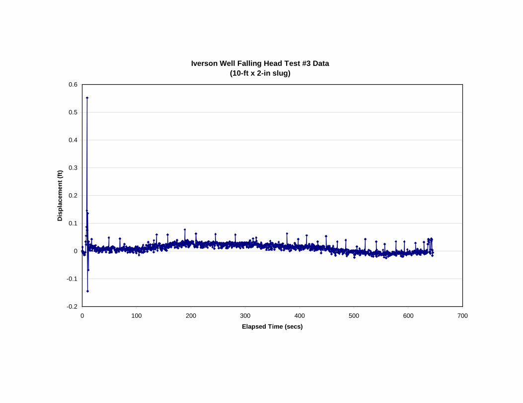
The Iverson well recovered too quickly to get a good, readable falling or rising head curve, so we can only say that the hydraulic conductivity was fairly high. Low conductivity will result in a curve that takes relatively longer to decay. However, in spite of considerable noise in the data, the first falling head test suggests that the hydraulic conductivity is on the order of 25 to 30 feet per day. This well was not included in the average for the revised models.

Parameters for analytical and numerical modeling

The average hydraulic conductivity (K) from the slug tests at the Herb Owens and Squirrel Spring wells was 13.4 feet per day. This was multiplied by an aquifer thickness of 200 feet to

give a transmissivity (T) of 2680 ft2/d, the number used in both models. The 200 foot thickness is from the lower range value used for the White Mountains and volcanic aquifers in the August 29, 2007 report. For the analytical model, values 20% higher and lower than this were also applied (3216 and 2144 ft2/d, respectively).

Storage characteristics of the aquifer are not obtainable from slug tests. This would require a longer pumping test, with adequate monitoring wells. However, the average range of specific yield values for unconfined aquifers ranges from 0.02 to 0.3 (Fetter, 1988). Williams and Soroos (1973) reported a range of specific yield values of 0.05 to 0.19 for unconfined volcanic aquifers from pumping tests performed on the island of Oahu, Hawaii. Specific yield is the ratio of water available for pumping from a volume of rock, divided by the total volume of rock. For this modeling effort, 0.05 was used in order to be conservative. A larger number, such as 0.1 would result in a smaller cone of depression since there would be a greater volume of water in a given volume of the aquifer.

Analytical model

The analytical model is identical with the model used in the August 29, 2007 report, with the exception of the newly refined transmissivity value. The Neuman (1972) solution for water table aquifers was used within the AquiferWin32 software package1

Figure 3 shows drawdown curves near the Little Colorado River by the Spinedace habitat (highlighted in blue near the town of Springerville) at monitoring well MW-SD (Figure 2), nine miles from the potential development. Transmissivities of 20% higher and lower than 2680 ft2/d are shown, and a 100 year drawdown of about 0.17 to 0.2 feet is the result.

. The 100 year cone of depression is shown in Figure 2. This model uses the assumption that the hydrogeologic characteristics of the aquifer are homogeneous and isotropic over the entire model domain; i.e., there is no variability anywhere. Also, the model implicitly assumes that, at the scale of the simulation, the aquifer behaves like porous media flow; fracture flow is not significant. There is also no interaction with surface or atmospheric waters. The model shows that drawdown near Springerville after pumping 129 acre feet per year constantly for 100 years would be about 0.2 feet. Drawdown one mile east of Tract B would be about 2 feet.

This type of modeling does not ordinarily take a number of factors into consideration. These are:

• There is no recharge in the model. This results in a continually growing cone of depression, since all water is taken from storage. It is never replenished. The 100 year simulation is comparable to a 100 year drought.

• There are no obstacles to flow, such as an impermeable fault. An infinitely long, impermeable barrier directly adjacent to the two tracts would have the maximum effect of doubling the depth of the cone of depression. A barrier this tight would be unlikely.

1 http://www.scisoftware.com/products/pumping-test-details/pumping-test-details.html

• The residents of the proposed development are not likely to be there year-round. If they should be half-year or quarter-year residents, the cone of depression would be correspondingly shallower.

• All residents would be disposing of household waste water by means of a septic system. The US Geological Survey routinely assumes that 50 to 75% of wastewater reporting to a septic tank ends up returning to the water table aquifer. According to Paul (2007) in a detailed study Rocky Mountain septic systems, 84% of septic inflow ended up recharging the aquifer. This would result in a much shallower cone of depression, proportional to the amount of such recharge.

• The project area is over 8000 feet in elevation and the local precipitation is in excess of 20 inches per year. Current residents rarely indulge in lawn irrigation, and the project residents are also unlikely to do so. This would also reduce their average water use.

Such a model is a superposition model, which shows what changes on the groundwater system can be expected by the pumping of interest. No other stresses are portrayed, and no account needs to be made for numerous unknown stresses (Reilly, 1987).

Numerical Model

To address the effect of recharge on the growth and ultimate size of the cone of depression, a numerical simulation scenario was constructed, similar to the one utilized in the August 29, 2007 report. MODFLOW-2000 was used (Harbaugh and others, 2000). Very low recharge rates of 0.05 to 0.5 inches per year were applied in a blanket fashion over the model domain. The cone of depression will grow only until the amount of recharge intercepted equals the volumetric rate of pumping. Therefore, the lower the recharge rate, the larger the ultimate footprint of the cone of depression.

Addition of Recharge

The analytical solutions given above show a continually growing cone of depression. After 100 years this results in some minor drawdown in the vicinity of Springerville, Arizona. This occurs because there is no recharge included in the analytical solutions. All water comes from storage in the aquifer with no replenishment. The numerical solution was done in order to give some idea of the effect recharge would have on the extent of the cone of depression.

Figure 4 shows the steady state footprint for the 0.5, 0.2, 0.1, and 0.05 inch recharge scenario. This amounts to 0.25 to 2.5% of the local average precipitation. Prudic and others (1995) used a value of 3% of total precipitation for their Great Basin model. It also does not take into account other forms of recharge from surface water infiltration from septic systems, streams, or lakes/reservoirs/ponds. In the case of the latter, this would ultimately result in a cumulative loss of flow to the Little Colorado river, since it would result in some loss of outflow from the reservoir.

Figure 5 shows the 100 year drawdown about 1 mile east of the proposed development for both the analytical solution and three of the numerical solutions; with 0.05, 0.1 and 0.2 inches of

annual recharge. The analytical cone of depression never stops growing because there is no recharge and all water is taken from storage. When recharge is added, the cone of depression only grows until it captures recharge or surface flow equal to the quantity of pumping. The numerical solutions reach a steady state level after about 10 years. The more recharge, the less drawdown when steady state is achieved.

Effects on Stream Flow in the Little Colorado River

In order to show some measure of potential effects to stream flow in the Little Colorado River, the numerical simulation was required. The MODFLOW model described above was used, with 0.1 inches per year aerially through the recharge package. This was applied in an average seasonal quantity, as given in the table below. Total precipitation averages about 22 inches per year, so application of 0.1 inch per year recharge (0.5%) is conservative. Also, 0.1 inch recharge for this project area was used by Papadopulos and Associates (2005) in their C aquifer model, although they considered recharge to the C aquifer alone. Three to five percent is commonly used for recharge in the southwest, which would be 0.7 to 1.1 inches per year. Prudic and others (1995) used 3% of total precipitation for their groundwater flow model of the Great Basin.

Seasonal Recharge Rates Pumping rate per well Winter 0.075 in/y 0.043 gpm Spring 0.044 in/y 0.31 gpm Summer 0.189 in/y 0.31 gpm Fall 0.092 in/y 0.043 gpm Average 0.10 in/y

The Draft EIS for the Black River Land Exchange reported that 14% of the current Greer area residents are present year round, and 86% are seasonal residents, generally being in the area from April through September. A pumping schedule was applied to the model reflecting these proportions, also shown in the table above. For winter and Fall, each well was decreased to 14% of the full rate, rather than to deactivate 86% of the wells. Fifty percent of the amount of water pumped from the development wells was recharged in the immediate area through MODFLOW’s recharge package. This represents septic tank effluent returned to the water table, though the proportion may be considerably higher (Paul, 2007).

Although the simulation ran out to 100 years, the overall drawdown stabilized after 3 years and did not vary from that time on. This happens when the cone of depression has grown to the point that it captures as much recharge, both from surface recharge and the river package, as the wells are pumping. Without recharge, the cone of depression never ceases to grow.

The river package of McDonald and Harbaugh (1988) was used to estimate the percentage loss of flow to the Little Colorado River after the method of Leake and others (2005). As it is a superposition model, only the pumping stresses of the possible development are represented. Because of this, whatever drawdown effects shown by this model would be directly additive to any other pumping stresses not represented. In this case, the river stage is set to zero feet elevation, the same level as the initial water table, so that the only effects on the river cells would be from pumping at the development. The river bed was set to a thickness of one foot. A thicker

river bed would lead to lesser impacts. The vertical hydraulic conductivity was set to 1 foot per day, the same value used by Leake and others (2005).

The result of including seasonality in recharge and pumping was to produce a periodicity in the level of the water table (Figure 6). This stabilized after about three years with no further net drawdown of the water table.

The Zonebudget module was run with MODFLOW to calculate water balances. The flow from the river cells to the aquifer, induced by the development pumping, was compared to the USGS stream gage at Greer, AZ (number 09383400) to calculate a percentage loss from the river. The seasonal results are given in the table below. With no recharge other than from the river, the average annual percent stream loss increases to about 1% of Little Colorado flow.

Winter Spring Summer Fall

Greer gage average (cfs) 7.72 36.82 12.71 5.33 River leakage from MODFLOW (cfs) 0.028 0.031 0.030 0.034 Percent stream loss 0.36% 0.08% 0.24% 0.64% Greer area average precipitation (in/y) 4.29 2.48 10.77 5.26

Figure 7 shows the average monthly flows in the Little Colorado River and average monthly precipitation at Greer.

Conclusions and observations

A 258-home development near Greer would likely affect the amount of flow in the Little Colorado river if the shallow White Mountain and volcanic aquifers were tapped for water supply. However, the total effect would be minimal. The slug tests performed in July of 2009 show that the aquifer is sufficiently transmissive to be a viable water supply for a development of this size, especially considering that few of the residents of such a development are likely to be there year-round.

Water consumption in the proposed development at full build-out would be approximately 74 acre feet per year, if residential frequency is similar to present rates of 14% year-round and 86% half-year, and assuming a 0.5 acre foot per year per full-time household consumption rate. The average annual flow in the Little Colorado river at Greer, from 1960 to 1982 was 15.6 cubic feet per second, or 11,300 acre feet per year. The development water use represents 0.2% of this average flow on an annual basis. The proportion of flow reduction, if any, near Springerville would be a smaller percentage because the Greer flow values do not take into account other contributions to Little Colorado river flow between Greer and Springerville, or the effect of septic tank return flow.

The residents of the proposed development will be utilizing septic tanks for domestic wastewater disposal. The USGS routinely considers that 50% to 75% of water reporting to the septic tank ends up recharging the water table aquifer (personal communication with Nathan Myers) and Paul (2007) reports a value of 84% of septic influx as recharge in Jefferson County, Colorado. This would reduce the percentage of pumping to Little Colorado River flow to between 0.57% to 0.18%.

Addition of seasonality to model recharge and water use resulted in loss of �ow to the Little Colorado River of between 0.08% to 0.64% depending on the season. Aquifer storage parameters, septic tank return �ow, and recharge quantities were kept on the conservative side to keep the model somewhat pessimistic. Seasonal residents would be present when �ow is at its maximum in the Little Colorado River or when precipitation is greatest.

Ultimately, there is little likelihood that a reduction in Little Colorado river �ow at Springerville, Arizona would be noticeable. Because there is a signi�cant amount of recharge to the aquifers in the Greer area (Papadopulos and Associates, Inc., 2005), the cone of depression is unlikely to extend much beyond the local area of the development.

References

Bouwer, H. and Rice, R.C., 1976. A slug test for determining hydraulic conductivity of unconfined aquifers with completely or partially penetrating wells. Water Resources Research, v. 12, n. 3, p. 423-428. Fetter, C.W., 1988. Applied Hydrogeology, second edition. 592 pp.

Harbaugh, A.W., Banta, E.R., Hill, M.C., and McDonald, M.G., 2000. MODFLOW–2000, the U.S. Geological Survey Modular Ground-Water Model—User guide to modularization concepts and the Ground-Water Flow Process: U.S. Geological Survey Open-File Report 00–92, 121 p.

Leake, S.A., J.P. Hoffmann, and Jesse E. Dickinson, 2005. Numerical ground-water change model of the C aquifer and effects of ground-water Withdrawals on stream depletion in selected reaches of Clear Creek, Chevelon Creek, and the Little Colorado River, northeastern Arizona, USGS Scientific Investigations Report 2005-5277, 39 p.

McDonald, M.G., and Harbaugh, A.W., 1988, A modular three-dimensional finite-difference ground-water flow model: U.S. Geological Survey Techniques of Water-Resources Investigations, book 6, chap. A1, 586 p.

Neuman, S.P., 1972. Theory of flow in unconfined aquifers considering delayed response of the water table. Water Resources Research, v. 8, n. 4, p. 1031-1045.

Papadopulos and Associates, Inc., 2005. Groundwater flow model of the C aquifer in Arizona and New Mexico. Prepared for the Salt River Project. 138 pp.

Paul, B., 2007, Water Budget of Mountain Residence: Colorado School of Mines, M.S. thesis, 68 pp.

Prudic, David E., James R. Harrill, and Thomas J. Burbey, 1995. Conceptual evaluation of regional ground-water flow in the carbonate-rock province of the Great Basin, Nevada, Utah, and adjacent states: U.S. Geological Survey Professional Paper 1409-D. 118 p.

Reilly, T.E., Franke, O. Lehn, and Bennett, G.D., 1987, The principle of superposition and its application in ground-water hydraulics: U.S. Geological Survey Techniques of Water-Resources Investigations Book 3, Chap. B6, 28 p.

Williams, J.A. and Soroos, R.L., 1973. Evaluation of methods of pumping test analysis for application to Hawaiian aquifers. Technical Report No. 70, Water Resources Research Center, University of Hawaii, Honolulu, HI. 159 pp.

Figure 1. Location map for wells used in slug tests.

Figure 2. The analytical 100 year cone of depression. The Neuman (1972) solution for unconfined aquifers was utilized.

Figure 3. The 100 year drawdown curve for modeled (fictional) monitoring well MW-SD shown in Figure 2 above. Pumping only from the proposed development was considered in this modeling. This would be an addition to all other pumping.

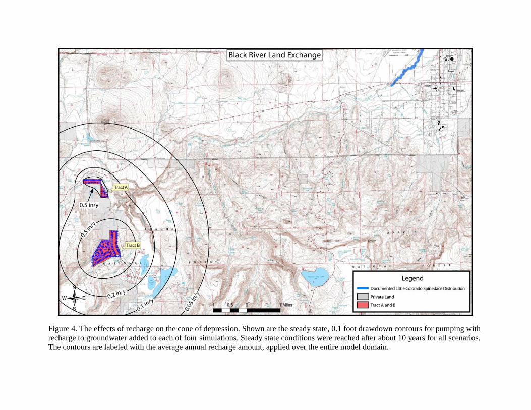
Figure 4. The effects of recharge on the cone of depression. Shown are the steady state, 0.1 foot drawdown contours for pumping with recharge to groundwater added to each of four simulations. Steady state conditions were reached after about 10 years for all scenarios. The contours are labeled with the average annual recharge amount, applied over the entire model domain.

Figure 5. 100 year Drawdown for a hypothetical monitoring well about one mile east of the proposed development (MW-4 in Figure 2). The curve labeled “without recharge” is the analytical solution. The other two (with recharge) are numerical solutions.

Figure 6. Periodicity in water table level due to season input for water use and recharge. The same pattern persists for the 100 years of the simulation, having stabilized after three years. This observation well was located in the center of Tract A.

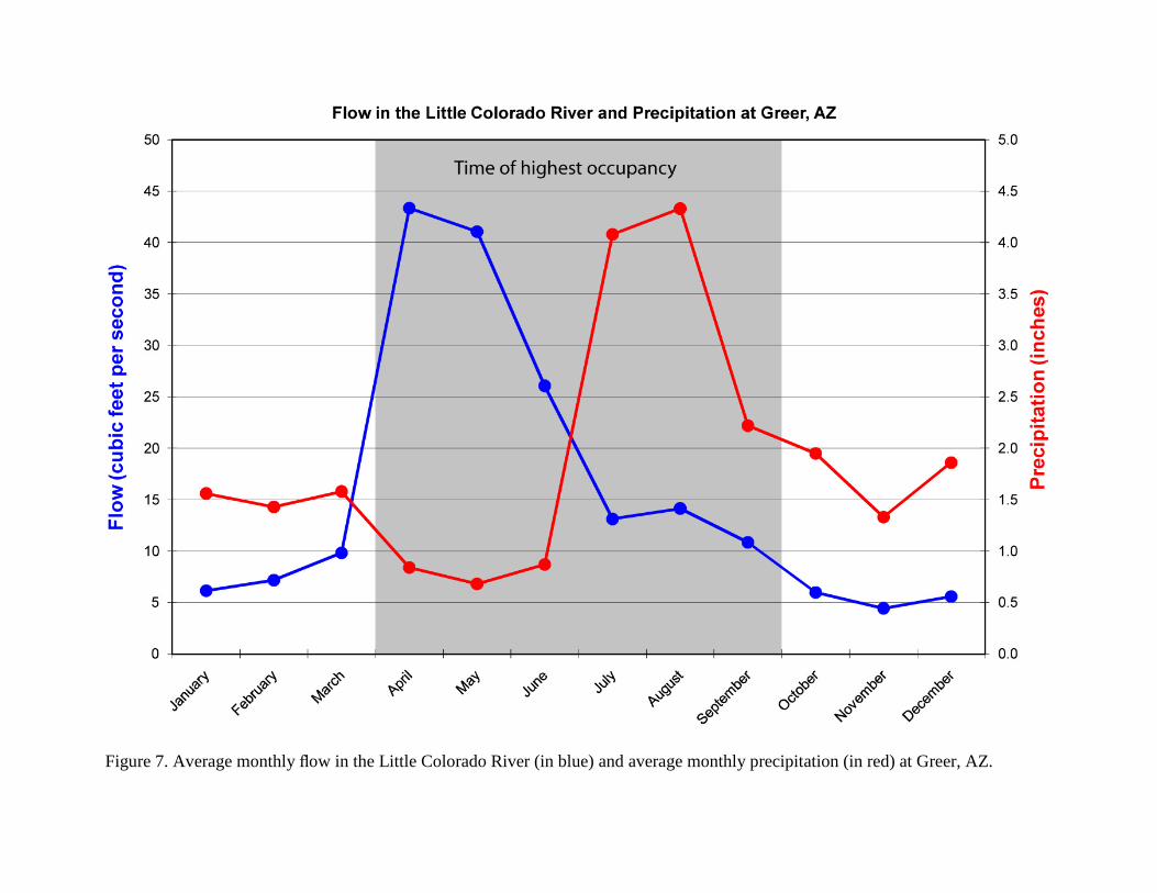
Figure 7. Average monthly flow in the Little Colorado River (in blue) and average monthly precipitation (in red) at Greer, AZ.

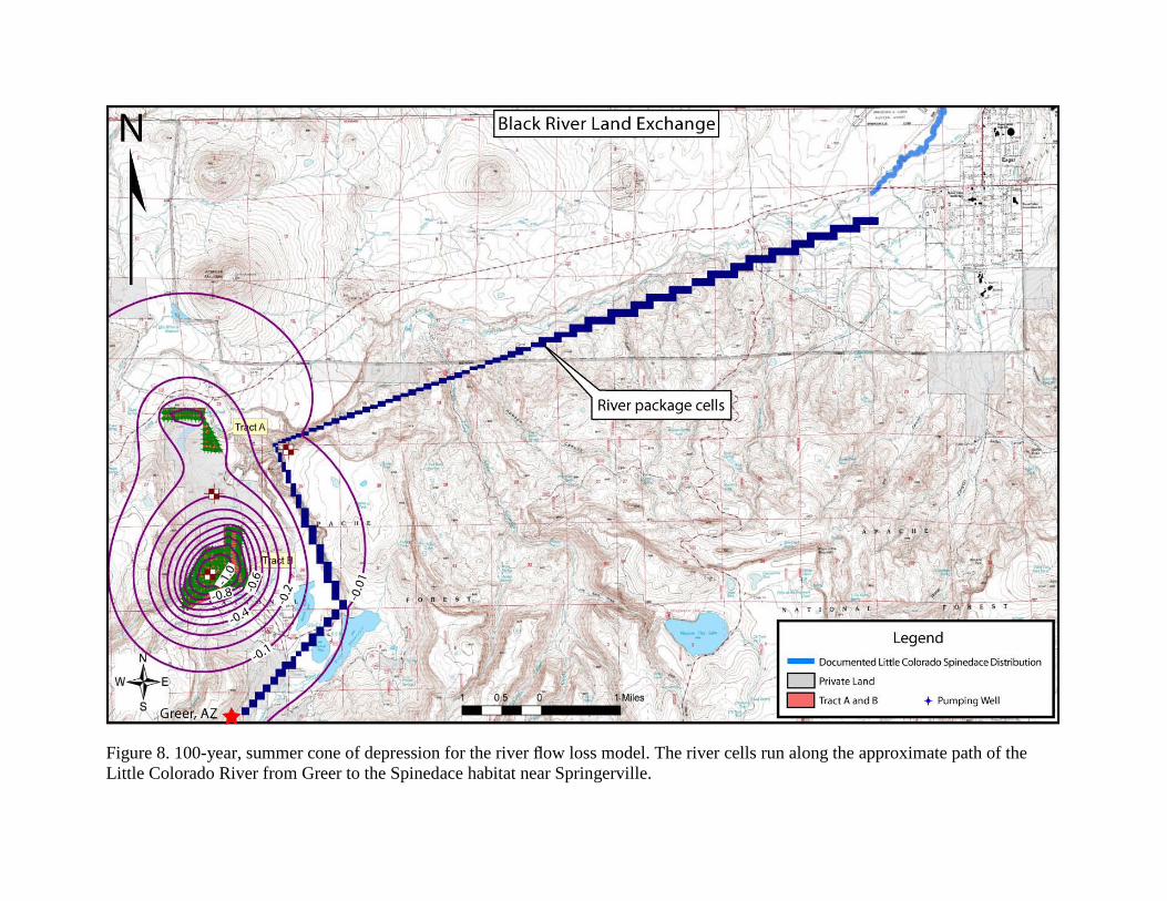
Figure 8. 100-year, summer cone of depression for the river flow loss model. The river cells run along the approximate path of the Little Colorado River from Greer to the Spinedace habitat near Springerville.

Appendix A

Data from DB Stephens and Associates

Squirrel Springs Well Falling Head Test #1 Data(10-ft x 4-in slug)

0

1

2

3

4

5

6

7

0 200 400 600 800 1000 1200 1400

Elapsed Time (secs)

Dis

plac

emen

t (ft)

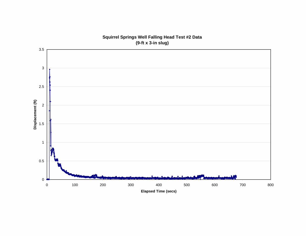
Squirrel Springs Well Falling Head Test #2 Data(9-ft x 3-in slug)

0

0.5

1

1.5

2

2.5

3

3.5

0 100 200 300 400 500 600 700 800

Elapsed Time (secs)

Dis

plac

emen

t (ft)

Squirrel Springs Well Falling Head Test #3 Data(10-ft x 4-in slug)

0

0.5

1

1.5

2

2.5

3

3.5

4

4.5

5

0 100 200 300 400 500 600 700 800 900 1000

Elapsed Time (secs)

Dis

plac

emen

t (ft)

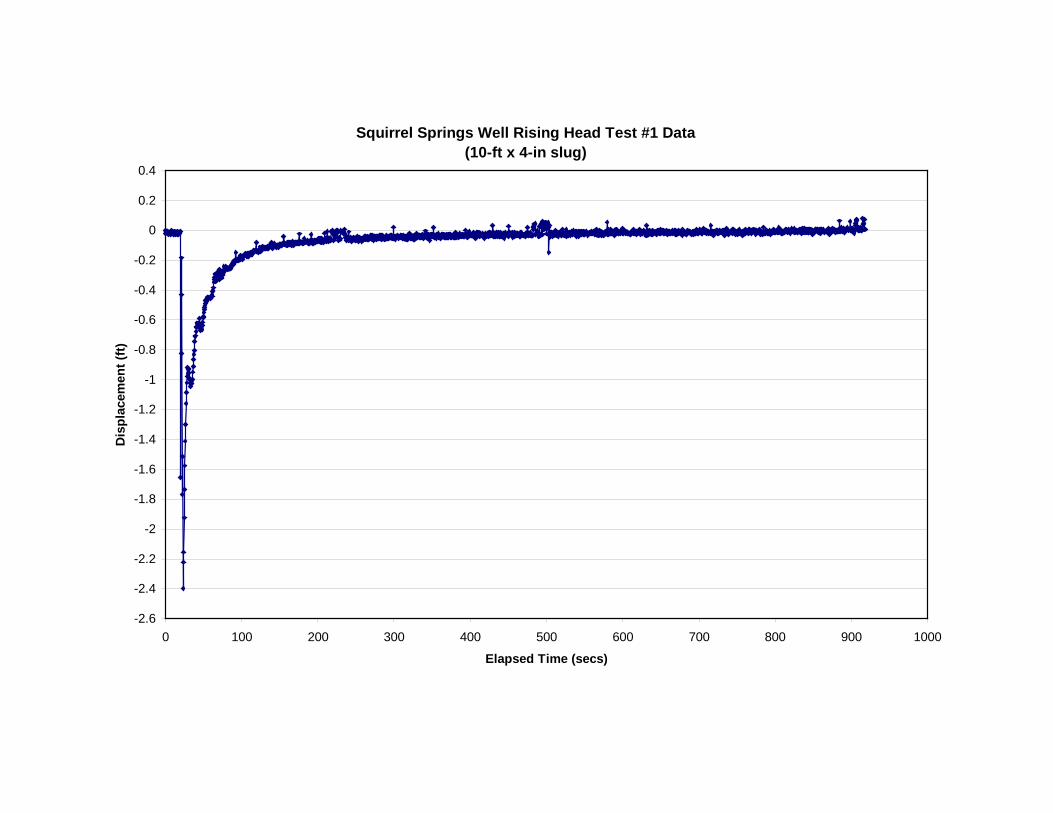
Squirrel Springs Well Rising Head Test #1 Data(10-ft x 4-in slug)

-2.6

-2.4

-2.2

-2

-1.8

-1.6

-1.4

-1.2

-1

-0.8

-0.6

-0.4

-0.2

0

0.2

0.4

0 100 200 300 400 500 600 700 800 900 1000

Elapsed Time (secs)

Dis

plac

emen

t (ft)

Squirrel Springs Well Rising Head Test #2 Data(9-ft x 3-in slug)

-2

-1.8

-1.6

-1.4

-1.2

-1

-0.8

-0.6

-0.4

-0.2

0

0.2

0 100 200 300 400 500 600 700 800 900 1000 1100 1200 1300 1400

Elapsed Time (secs)

Dis

plac

emen

t (ft)

Squirrel Springs Well Rising Head Test #3 Data(10-ft x 4-in slug)

-2.4

-2.2

-2

-1.8

-1.6

-1.4

-1.2

-1

-0.8

-0.6

-0.4

-0.2

0

0.2

0.4

0.6

0 100 200 300 400 500 600 700 800 900 1000

Elapsed Time (secs)

Dis

plac

emen

t (ft)

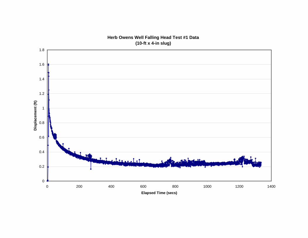
Herb Owens Well Falling Head Test #1 Data(10-ft x 4-in slug)

0

0.2

0.4

0.6

0.8

1

1.2

1.4

1.6

1.8

0 200 400 600 800 1000 1200 1400

Elapsed Time (secs)

Dis

plac

emen

t (ft)

Herb Owens Well Falling Head Test #2 Data(10-ft x 4-in slug)

0

0.5

1

1.5

2

2.5

3

0 200 400 600 800 1000 1200 1400 1600 1800 2000

Elapsed Time (secs)

Dis

plac

emen

t (ft)

Herb Owens Well Falling Head Test #3 Data(5-ft x 4-in slug)

0

0.2

0.4

0.6

0.8

1

1.2

1.4

1.6

0 200 400 600 800 1000 1200 1400 1600 1800 2000

Elapsed Time (secs)

Dis

plac

emen

t (ft)

Herb Owens Well Falling Head Test #4 Data(10-ft x 4-in slug)

0

0.5

1

1.5

2

2.5

0 200 400 600 800 1000 1200 1400

Elapsed Time (secs)

Dis

plac

emen

t (ft)

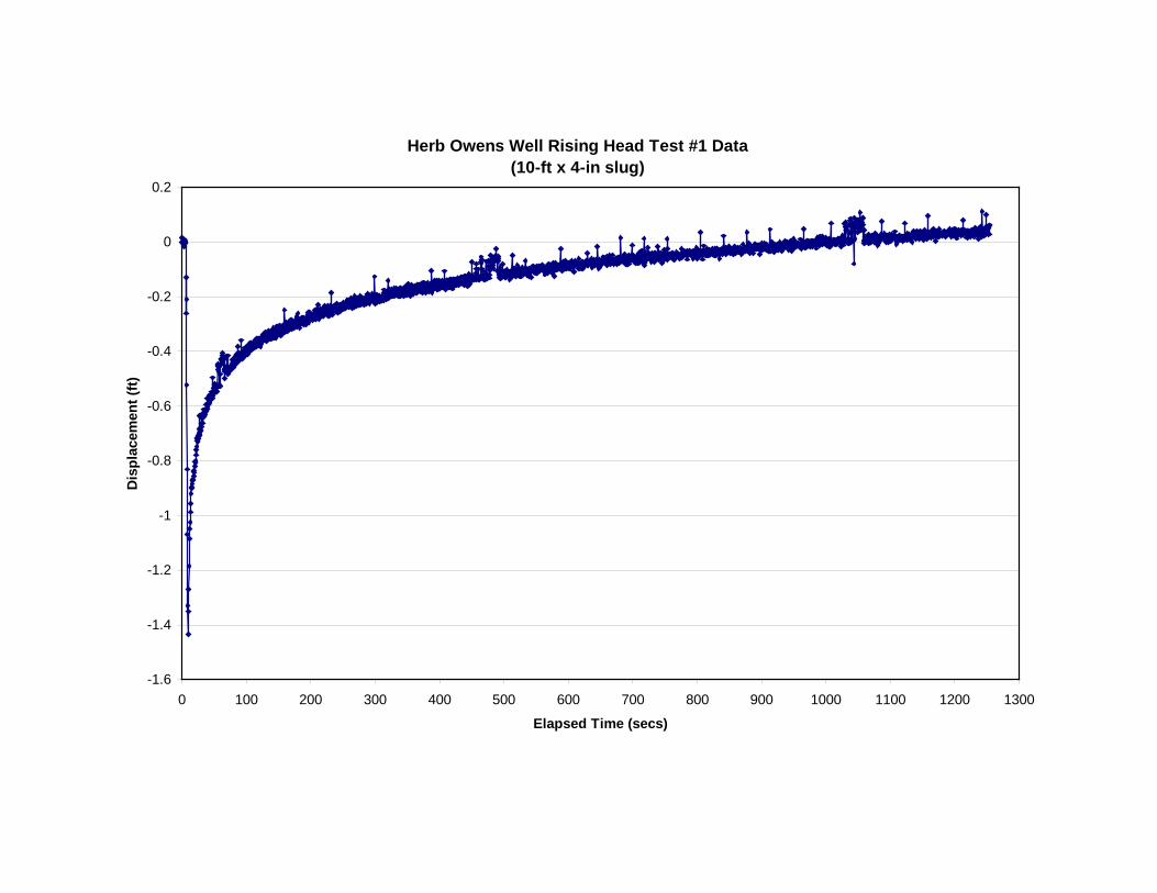
Herb Owens Well Rising Head Test #1 Data(10-ft x 4-in slug)

-1.6

-1.4

-1.2

-1

-0.8

-0.6

-0.4

-0.2

0

0.2

0 100 200 300 400 500 600 700 800 900 1000 1100 1200 1300

Elapsed Time (secs)

Dis

plac

emen

t (ft)

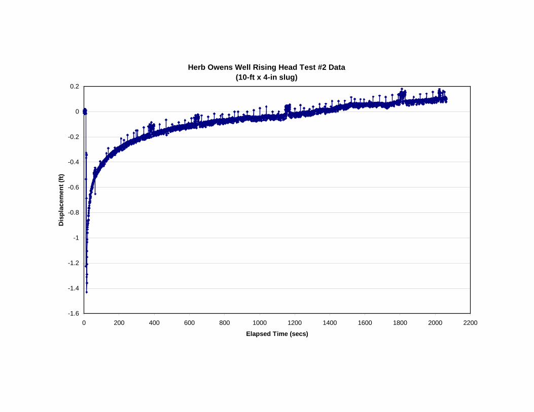
Herb Owens Well Rising Head Test #2 Data(10-ft x 4-in slug)

-1.6

-1.4

-1.2

-1

-0.8

-0.6

-0.4

-0.2

0

0.2

0 200 400 600 800 1000 1200 1400 1600 1800 2000 2200

Elapsed Time (secs)

Dis

plac

emen

t (ft)

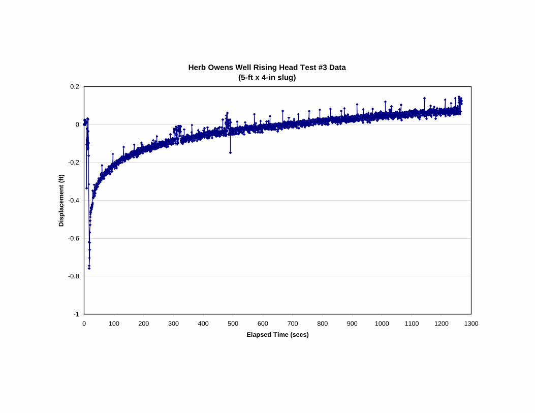
Herb Owens Well Rising Head Test #3 Data(5-ft x 4-in slug)

-1

-0.8

-0.6

-0.4

-0.2

0

0.2

0 100 200 300 400 500 600 700 800 900 1000 1100 1200 1300

Elapsed Time (secs)

Dis

plac

emen

t (ft)

Herb Owens Well Rising Head Test #4 Data(10-ft x 4-in slug)

-1.6

-1.4

-1.2

-1

-0.8

-0.6

-0.4

-0.2

0

0.2

0 200 400 600 800 1000 1200 1400 1600 1800 2000 2200 2400 2600 2800 3000 3200 3400

Elapsed Time (secs)

Dis

plac

emen

t (ft)

Iverson Well Falling Head Test #1 Data(10-ft x 2-in slug)

-0.1

-0.05

0

0.05

0.1

0.15

0.2

0 100 200 300 400 500 600 700 800 900

Elapsed Time (secs)

Dis

plac

emen

t (ft)

Iverson Well Falling Head Test #2 Data(10-ft x 2-in slug)

-0.1

-0.05

0

0.05

0.1

0.15

0.2

0 50 100 150 200 250 300

Elapsed Time (secs)

Dis

plac

emen

t (ft)

Iverson Well Falling Head Test #3 Data(10-ft x 2-in slug)

-0.2

-0.1

0

0.1

0.2

0.3

0.4

0.5

0.6

0 100 200 300 400 500 600 700

Elapsed Time (secs)

Dis

plac

emen

t (ft)

Iverson Well Falling Head Test #4 Data(10-ft x 2-in slug)

-0.6

-0.4

-0.2

0

0.2

0.4

0.6

0 20 40 60 80 100 120 140 160 180 200

Elapsed Time (secs)

Dis

plac

emen

t (ft)

Iverson Well Rising Head Test #1 Data(10-ft x 2-in slug)

-0.5

-0.4

-0.3

-0.2

-0.1

0

0.1

0 100 200 300 400 500 600

Elapsed Time (secs)

Dis

plac

emen

t (ft)

Iverson Well Rising Head Test #2 Data(10-ft x 2-in slug)

-0.2

-0.15

-0.1

-0.05

0

0.05

0.1

0 100 200 300

Elapsed Time (secs)

Dis

plac

emen

t (ft)

Iverson Well Rising Head Test #3 Data(10-ft x 2-in slug)

-0.3

-0.2

-0.1

0

0.1

0 100 200 300 400

Elapsed Time (secs)

Dis

plac

emen

t (ft)

Iverson Well Rising Head Test #4 Data(10-ft x 2-in slug)

-0.4

-0.3

-0.2

-0.1

0

0.1

0 100 200 300

Elapsed Time (secs)

Dis

plac

emen

t (ft)