Ambiguity, Monetary Policy and Trend

Inflation∗

Riccardo M. Masolo Francesca Monti

Bank of England and CfM

March 19, 2018

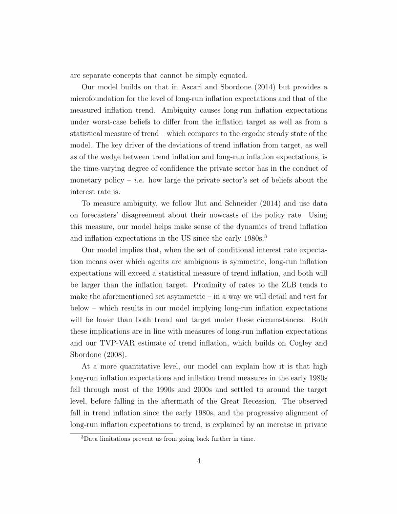
Abstract

Allowing for ambiguity about the behavior of the policymaker ina simple new-Keynesian model gives rise to wedges between long-runinflation expectations, trend inflation, and the inflation target. Thedegree of ambiguity we measure in Blue Chip survey data helps explainthe dynamics of long-run inflation expectations and the inflation trendmeasured in the US data. Ambiguity also has implications for monetarypolicy. We show that it is optimal for policymakers to lean against thehouseholds’ pessimistic expectations, but also document the limits tothe extent the adverse effects of ambiguity can be undone.JEL Classification: D84, E31, E43, E52, E58Keywords: Ambiguity aversion, monetary policy, trend inflation, in-flation expectations

∗Previously circulated as Monetary Policy with Ambiguity Averse Agents. We are gratefulto our discussants J. Costain, C. Ilut, P. Karadi and A. Sbordone, and to G. Ascari, C.Carvalho, F. De Graeve, W. Den Haan, J. Fernandez-Villaverde, R. Harrison, R. Meeks, R.Reis and P. Santos Monteiro for insightful comments and suggestions. We would also like tothank seminar participants at Oxford University, Bank of Finland, ECB-WGEM, Bank ofKorea, Bank of England, Bank of Canada, University of York and King’s College London,as well as participants at the 2015 North American Winter Meeting of the EconometricSociety, the 2015 Barcelona GSE Summer Forum, the Cleveland Fed 2016 Inflation: Driversand Dynamics Conference, and the 2016 Mid-Year NBER EFSF group Workshop at theChicago Fed. Any views expressed are solely those of the authors and so cannot be taken torepresent those of the Bank of England or to state Bank of England policy.

1

1 Introduction

The private sector’s expectations about monetary policy are key determinants

of economic outcomes. Private agents make the economic decisions that de-

termine inflation and output. Their confidence in the conduct of monetary

policy is thus instrumental to the success of the policy itself. We are now far

removed from the times in which monetary policy was perceived as an arcane

undertaking best practiced out of public view,1 and transparency has become

a key tenet of modern central banking. And yet, as the quote below notes, it is

practically impossible to completely eliminate uncertainty about the conduct

of monetary policy.

... the faulty estimate was largely attributable to misapprehensions about

the Fed’s intentions. [...] Such misapprehensions can never be eliminated, but

they can be reduced by a central bank that offers markets a clearer vision of its

goals, its ‘model’ of the economy, and its general strategy.

Blinder (1998)

In this paper we study how these misgivings can impact the effectiveness of

monetary policy in anchoring inflation expectations at the target level. And,

in particular, we show how the evolution of long-run inflation expectations over

the last 30 plus years can be explained by the increased degree of confidence

the private sector has regarding the conduct of monetary policy.

To do so, we build a model that explicitly allows for multiple priors about

the monetary policy rule, as a way of formalizing the misapprehensions dis-

cussed above in Blinder (1998). In particular, we augment a prototypical

new-Keynesian model by introducing ambiguity about the monetary policy

rule and assuming that agents are averse to ambiguity. Agents in our model

lack the confidence to assign probabilities to all relevant events. Rather, they

entertain as possible a set of multiple beliefs. Together with their strict pref-

erence for knowing probabilities, this implies that they act as if they evaluated

1As Bernanke pointed out in a 2007 speech: Montagu Norman, the Governor of theBank of England from 1921 to 1944, reputedly took as his personal motto, “Never explain,never excuse.”

2

plans based on the worst in their set of beliefs. We use a recursive version of

the multiple prior preferences (see Gilboa and Schmeidler, 1989, and Epstein

and Schneider, 2003), pioneered in business cycle models by Ilut and Schnei-

der (2014) and used, for example, by Baqaee (2015) to model how asymmetric

responses to news can explain downward wage rigidity.

The assumption that agents are not fully confident about the conduct of

monetary policy helps explain features of the data that are otherwise difficult

to make sense of. We focus on three. First, our model provides a rationale

for the observed low-frequency component in the series for inflation (inflation

trend) and its relationship with the inflation target. Second, it is able to cap-

ture the dynamics of long-run inflation expectations and to provide a rationale

for why, as Chan, Clark and Koop (2017) suggest, they differ from both the

target and the inflation trend. Third, we show that, in this class of models,

policymakers can do better than simply tracking the natural rate of interest.

Trend inflation and inflation expectations. The dynamics of inflation

and, in particular, its persistence are driven in large part by a low-frequency,

or trend, component, as documented for example in Stock and Watson (2007)

and Cogley and Sbordone (2008). Most of the macroeconomic literature re-

lies, however, on models that are approximated around a zero-inflation steady

state2 and that, consequently, cannot capture the persistent dynamic proper-

ties of inflation and long-run inflation expectations, nor their relationship. In

these models, the target, trend inflation and inflation expectations all coincide.

A strand of the macroeconomic literature, summarized in Ascari and Sbor-

done (2014), studies the effects of a trend in inflation by allowing for a time-

varying steady state level of inflation. This results in what they refer to as

a Generalized New-Keynesian Phillips and helps make sense of inflation per-

sistence. The model studied by Ascari and Sbordone (2014) treats inflation

trend as a primitive (taken from time-series estimates) and implies that long-

run inflation expectations will equal the inflation trend. Chan, Clark and

Koop (2017), however, show that long-run inflation expectations and trend

2Or alternatively, and equivalently from this perspective, a full indexation steady-state.

3

are separate concepts that cannot be simply equated.

Our model builds on that in Ascari and Sbordone (2014) but provides a

microfoundation for the level of long-run inflation expectations and that of the

measured inflation trend. Ambiguity causes long-run inflation expectations

under worst-case beliefs to differ from the inflation target as well as from a

statistical measure of trend – which compares to the ergodic steady state of the

model. The key driver of the deviations of trend inflation from target, as well

as of the wedge between trend inflation and long-run inflation expectations, is

the time-varying degree of confidence the private sector has in the conduct of

monetary policy – i.e. how large the private sector’s set of beliefs about the

interest rate is.

To measure ambiguity, we follow Ilut and Schneider (2014) and use data

on forecasters’ disagreement about their nowcasts of the policy rate. Using

this measure, our model helps make sense of the dynamics of trend inflation

and inflation expectations in the US since the early 1980s.3

Our model implies that, when the set of conditional interest rate expecta-

tion means over which agents are ambiguous is symmetric, long-run inflation

expectations will exceed a statistical measure of trend inflation, and both will

be larger than the inflation target. Proximity of rates to the ZLB tends to

make the aforementioned set asymmetric – in a way we will detail and test for

below – which results in our model implying long-run inflation expectations

will be lower than both trend and target under these circumstances. Both

these implications are in line with measures of long-run inflation expectations

and our TVP-VAR estimate of trend inflation, which builds on Cogley and

Sbordone (2008).

At a more quantitative level, our model can explain how it is that high

long-run inflation expectations and inflation trend measures in the early 1980s

fell through most of the 1990s and 2000s and settled to around the target

level, before falling in the aftermath of the Great Recession. The observed

fall in trend inflation since the early 1980s, and the progressive alignment of

long-run inflation expectations to trend, is explained by an increase in private

3Data limitations prevent us from going back further in time.

4

sector confidence, which in turn can be traced back to the great increase

in transparency and communications enacted by the Fed, as highlighted by

Lindsey (2003).

Work by Swanson (2006) supports this claim by showing that, since the

late 1980s, the cross-sectional dispersion of interest rate forecasts by U.S. fi-

nancial markets and private sector forecasters – i.e. their disagreement –

shrank and, importantly, by providing evidence that these phenomena can be

traced back to increases in central bank transparency. Similarly, Ehrmann,

Eijffinger and Fratzscher (2012) find that increased central bank transparency

lowers disagreement among professional forecasters. This seems natural. For

a given degree of uncertainty about the state of the economy, improved knowl-

edge about the policymakers’ objectives and model will make forecasters more

confident about monetary policy and their predictions more homogeneous. As

confidence in the conduct of monetary policy increases, our model implies that

long-run inflation expectations will approach the target.

Monetary Policy Implications. If the policymaker could dispel ambiguity

completely, it would be optimal to do so. It is however natural to imagine that

there is a limit to the extent to which Knightian uncertainty can be reduced.

For example, the changing composition of the policymaking committee might

introduce some uncertainty about the conduct of monetary policy in the future.

Our model generates interesting prescriptions for monetary policy in the

presence of ambiguity and can help make sense of policy actions, such as the

perceived excessive tightening early in the Volker tenure (Goodfriend, 2005).

In a situation like that of the early 1980s, characterized by high degree of

ambiguity and inflation above target, our model implies that the policymaker

should be more hawkish than what would be optimal in the absence of am-

biguity. In particular, the policymaker should increase its responsiveness to

inflation and, on top of that, should set the intercept of its policy rule above

the natural rate of interest. On the contrary, in situations in which ambiguity

drives long-run inflation expectations because of the proximity of the ZLB, it

is optimal for policymakers to aim for a rate below the natural rate of interest.

5

Our paper to work by Benigno and Paciello (2014), who consider optimal

monetary policy in a model in which agents have a desire for robustness to

misspecification about the state of the economy, in the spirit of Hansen and

Sargent (2007). The advantage of the multiple-priors approach is that we can

characterize the effects of ambiguity on the steady state.

The rest of the paper is organized as follows. Section 2 provides a descrip-

tion of the model we use for our analysis and characterizes the steady state

of our economy as a function of the degree of ambiguity. In Section 3 we

show how our simple model can match the dynamics of trend inflation, while

in Section 4 we discuss the implications for monetary policy of the presence

of some unavoidable Knightian uncertainty about monetary policy. Section 5

concludes.

2 The Model

We augment a simple New-Keynesian model (see Yun, 2005 or Galı, 2008)

by assuming that private agents face ambiguity about the expected future

policy rate. To isolate the effects of ambiguity, we set up our model so that,

absent ambiguity, the first-best steady state would be attained, thanks to a

government subsidy that corrects the distortion introduced by monopolistic

competition. Ambiguity, however, will cause worst-case steady-state inflation

to deviate from its target. For expositional simplicity, the derivation of the

model is carried out assuming the inflation target is zero, so the steady-state

level of inflation we find should be interpreted as a deviation from the target.

However, the model is equivalent to one in which the central bank targets a

positive constant level of inflation, to which firms index their prices.

We present the model’s building blocks starting with a description of the

monetary policy rule, which is critical for our analysis.

Monetary policy. In our economy the only disturbance unrelated to the

policymaker’s behavior is a technology shock At. A policy rule responding

6

more than one for one to inflation and including the natural rate of interest,

Rnt = Et

(At+1

βAt

), would thus be optimal (Galı, 2008). Indeed, together with

the optimal production subsidy, this policy rule would attain the first-best

allocation at all times.

However, we augment the policy rule to account for the possibility that the

policymaker might deviate from the rule or might follow a poorly measured

estimate of the natural rate of interest:

Rt =(Rnt e

ζt+1)

(Πt)φ , (1)

where ζt+1 is characterized by the following law of motion:

ζt+1 = ρζζt + uζt+1 + µt 0 < ρζ < 1 (2)

which would be a standard AR(1) process if it wasn’t for the presence of µt.

This formulation of the disturbance process serves multiple purposes. First, it

captures the idea that a deviation from the optimal rule today also represents

a signal of future likely deviations from the rule, which, for example, can be

thought of as capturing serial correlation in the mismeasurement of the natural

rate. Second, it captures autocorrelation in the policy rate, while not breaking

the result that, in the absence of this disturbance, the policy rule is such that

the economy attains first-best.4

Finally, it is important to note that the realization of ζt+1 is not known

at the time decisions are made a time t, and therefore agents are required to

compute expectations regarding the conduct of monetary policy. This is con-

sistent with the assumption adopted when identifying monetary policy shocks

with timing restrictions as in Christiano, Eichenbaum and Evans (2005). Also,

if monetary policy committees meet several times a quarter (twice a quarter

in the US), agents have to make predictions about the policymakers’ decisions

4A literature going back to Rudebush (2002) has discussed whether this formulation ispreferable to one in which the lagged policy rate enters the right-hand side of the policy rule.The optimality of the response to technological shocks and tractability considerations - thisformulation allows us to compute the solution to the log-linear approximation analytically- make us opt for this specification.

7

even within a quarter. In practice, so long as any relevant economic decision

has to be made prior to the last policy meeting of the quarter, our specifica-

tion captures a relevant economic situation faced by the private sector. And,

indeed, this uncertainty is evident in the survey data we use to measure ambi-

guity, namely the nowcast (forecast for the current quarter) of the Fed Funds

rate reported in the second month of the quarter in the Blue Chip survey.

From this perspective, ρζ captures the predictability of future deviations of

rates from the underlying optimal rule.

When it comes to the interpretation of µ, we follow Ilut and Schneider

(2014) and posit that the two terms that make up the innovations to ζt, zt+1 ≡ζt+1− ρζζt, are a sequence of i.i.d. Gaussian innovations uζt+1 ∼ N (0, σu), and

a deterministic sequence µt. By assumption, the empirical moments of µt

converge in the long run to those of an i.i.d. zero-mean Gaussian process,

independent of uζt+1, and with variance σ2z − σ2

u > 0, which result in µt being

extremely hard to recover.

Agents thus treat that term as ambiguous. The information at their dis-

posal only enables them to put bounds on their conditional expectations for

policy rates,5 which we parametrize with the interval [µt, µt].

6 The width of

the interval [µt, µt] measures the agents’ confidence, a smaller interval captur-

ing the idea that agents are more confident in their prediction of the policy

rate.

Households. The representative household’s felicity function is a function

of consumption Ct and hours worked Nt:

u(Ct, Nt) = log(Ct)−N1+ψt

1 + ψ,

5Given our timing convention, the realization of ζt+1 only becomes known after decisionsare made.

6Throughout the paper, we will maintain the assumption that µt< 0 and µt > 0 so

that the rational expectations model (µt = 0) is nested.

8

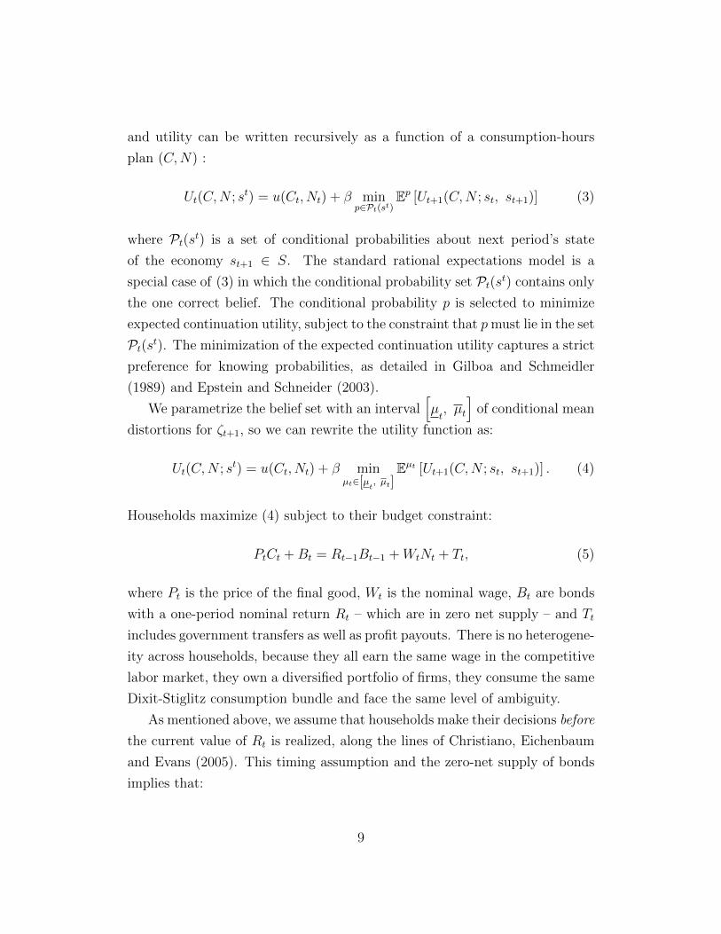
and utility can be written recursively as a function of a consumption-hours

plan (C,N) :

Ut(C,N ; st) = u(Ct, Nt) + β minp∈Pt(st)

Ep [Ut+1(C,N ; st, st+1)] (3)

where Pt(st) is a set of conditional probabilities about next period’s state

of the economy st+1 ∈ S. The standard rational expectations model is a

special case of (3) in which the conditional probability set Pt(st) contains only

the one correct belief. The conditional probability p is selected to minimize

expected continuation utility, subject to the constraint that pmust lie in the set

Pt(st). The minimization of the expected continuation utility captures a strict

preference for knowing probabilities, as detailed in Gilboa and Schmeidler

(1989) and Epstein and Schneider (2003).

We parametrize the belief set with an interval[µt, µt

]of conditional mean

distortions for ζt+1, so we can rewrite the utility function as:

Ut(C,N ; st) = u(Ct, Nt) + β minµt∈[µt, µt]

Eµt [Ut+1(C,N ; st, st+1)] . (4)

Households maximize (4) subject to their budget constraint:

PtCt +Bt = Rt−1Bt−1 +WtNt + Tt, (5)

where Pt is the price of the final good, Wt is the nominal wage, Bt are bonds

with a one-period nominal return Rt – which are in zero net supply – and Tt

includes government transfers as well as profit payouts. There is no heterogene-

ity across households, because they all earn the same wage in the competitive

labor market, they own a diversified portfolio of firms, they consume the same

Dixit-Stiglitz consumption bundle and face the same level of ambiguity.

As mentioned above, we assume that households make their decisions before

the current value of Rt is realized, along the lines of Christiano, Eichenbaum

and Evans (2005). This timing assumption and the zero-net supply of bonds

implies that:

9

1. At the beginning of time t, when decisions are made, the realization of ζt+1

is not yet known, so the household’s expected policy rate (substituting

the expectation into (1) and taking logs) is:

Eµtt rt = rnt + ρζζt + µt + φπt.

2. Consumption will be pinned down so that desired savings are zero, given

this expectation for the policy rate (which is common across all house-

holds).

3. When the actual policy rate is set, it will not affect households wealth,

because bond holdings are zero.

The household’s intertemporal and intratemporal Euler equations are thus:

1

Ct= Eµtt

[βRt

Ct+1Πt+1

](6)

Nψt Ct =

Wt

Pt. (7)

We can rewrite the intertemporal Euler equation substituting in the distorted

expectations for the policy rate:

1

Ct= Et

[βRn

t eρζζt+µt (Πt)

φ

Ct+1Πt+1

], (8)

where Et is the rational expectations operator. Equations (7) and (8) charac-

terize the maximization problem of the households. We will turn to finding

the level of µt that solves the minimization problem in the next section.

Firms. The final good Yt is produced by perfectly competitive producers us-

ing a continuum of intermediate goods Yt(i) and the standard CES production

function

Yt =

[∫ 1

0

Yt(i)ε−1ε di

] εε−1

. (9)

10

Taking prices as given, the final good producers choose intermediate good

quantities Yt(i) to maximize profits, resulting in the usual Dixit-Stiglitz de-

mand function for intermediate goods

Yt(i) =

(Pt(i)

Pt

)−εYt (10)

and in the aggregate price index

Pt =

[∫ 1

0

Pt(i)1−εdi

] 11−ε

.

Intermediate goods are produced by a continuum of monopolistically com-

petitive firms using the following linear technology:

Yt(i) = AtNt(i), (11)

where At is a stationary technology process. Prices are sticky in the sense of

Calvo (1983): only a random fraction (1 − θ) of firms can re-optimize their

price in any given period. Whenever a firm can re-optimize, it sets its price

maximizing the expected presented discounted value of future profits

maxP ∗t (i)

∞∑s=0

θjβjE

[C−1t+j

Pt+j

[P ∗t Yt+j(i)− Pt+jMCt+jYt+j(i)

]], (12)

where MCt = (1− τ) Wt

AtPtis the real marginal cost, net of the subsidy τ = 1/ε.

The firm’s price-setting decision, which is the same for all the firms setting

prices in given period, can be characterized by the firms’ first-order condition7

P ∗t (i)

Pt=

εε−1

Et∑∞

j=0 βjθjMCt+j

(PtPt+j

)−εEt∑∞

j=0 βjθj(

PtPt+j

)1−ε (13)

7Log-preferences in consumption and the fact that Yt = Ct simplify this expression asthe marginal utility of future consumption simplifies out with aggregate output in the profitfunction.

11

together with the following equation derived from the law of motion for the

price index:

P ∗t (i)

Pt=

(1− θΠε−1

t

1− θ

) 11−ε

. (14)

Government and Market Clearing. The Government runs a balanced

budget and finances the production subsidy with a lump-sum tax. Out of

notational convenience, we include the firms’ aggregate profits in the lump-

sum transfer:

Tt = Pt

[−τ Wt

PtNt + Yt

(1− (1− τ)

Wt∆t

PtAt

)]= PtYt

(1− Wt∆t

PtAt

).

where ∆t is the price dispersion term, which we define below.

Market clearing in the goods markets requires that Yt(i) = Ct(i) for all

firms i ∈ [0, 1] and all t, which implies

Yt = Ct.

Market clearing on the labor market implies that

Nt =

∫ 1

0

Nt(i)di =

∫ 1

0

Yt(i)

Atdi =

YtAt

∫ 1

0

(Pt(i)

Pt

)−εdi,

where we define ∆t ≡∫ 1

0

(Pt(i)Pt

)−εdi as the relative price dispersion across

intermediate firms (Yun, 2005).

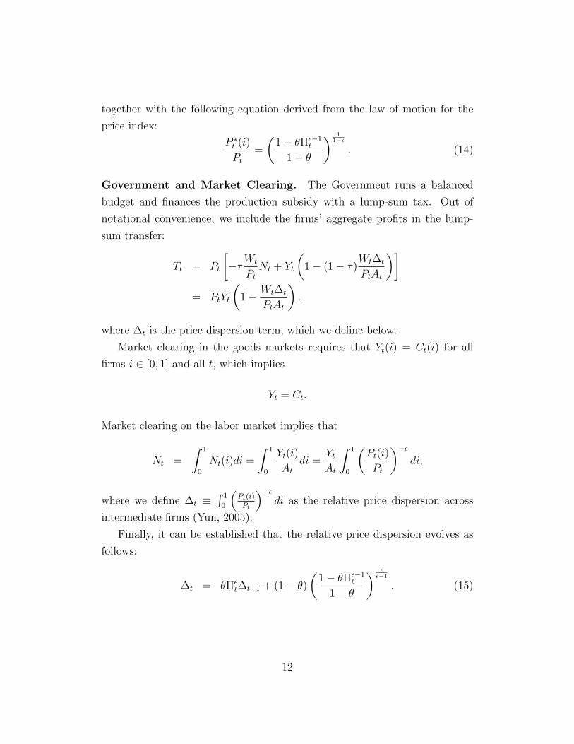
Finally, it can be established that the relative price dispersion evolves as

follows:

∆t = θΠεt∆t−1 + (1− θ)

(1− θΠε−1

t

1− θ

) εε−1

. (15)

12

2.1 Steady State

We study our model economy around the worst-case steady state, since agents

act as if the economy converges there in the long run (see Ilut and Schneider,

2014). The agents’ pessmistic expectations however are not fulfilled by the

realization of the exogenous process, so in general the ergodic steady state will

differ from its worst-case counterpart. We will discuss both steady states in

turn.

We derive the steady state of the agents’ first-order conditions as a function

of a generic level of the belief distortion induced by ambiguity, µ, and we

then rank the different steady states, indexed by µ, to characterize the worst-

case steady state. To keep notation to a minimum, we will define worst-case

steady-state variables as having no time subscript,8 even though we will later

on give an anticipated-utility (Kreps, 1998 and Cogley and Sargent, 2008)

interpretation to these quantities, in the tradition of Cogley and Sbordone

(2008).Finally it is convenient to collect parameter values by defining

ω =[β, ε, θ, φ, ρζ , ρa, ψ

]. The set of admissible parameter values can then

be characterized as:

Ω =ω :(β ∈ (0, 1), ε ∈ (1,∞), θ ∈ (0, 1), φ ∈ (1,∞), ρζ ∈ (0, 1), ρa ∈ (0, 1), ψ ∈ [0,∞)

)∩

(ρζ +

εµ

log (θ) (φ− 1)< 1

). (16)

The first part of the definition of Ω simply includes the standard economic

restrictions on the discount factor, the demand elasticity, the probability of

firms not being able to reset prices, the responsiveness of monetary policy to

inflation deviations from target (assuming the Taylor principle is satisfied), the

autocorrelation coefficients for the two exogenous processes and the inverse

Frish elasticity, respectively. The second part of the definition restricts a

combination of parameter values to ensure the steady state is well defined.9

This condition does not restrict the set of admissible paramters at all for µ = 0

8With the understanding that setting µ = 0 in those expressions delivers the first-beststeady state.

9As shown in Appendix A, this condition ensures that N (µ, ω) > 0 and real.

13

and becomes more restrictive as the degree of ambiguity increases. In practice,

we will only use it in the context of our estimation exercise by checking that

it is met by estimated parameters.

Worst-Case Steady State. We can divide the presentation of the worst-

case steady state into two separate parts. We start by expressing inflation as

a function of a generic perceived value of the disturbance ζ in steady state.

All other steady state variables can be then computed as a function of steady-

state inflation in a way that mimics that of the trend inflation literature (e.g.

Ascari and Ropele, 2009).

Proposition 2.1. In a steady state in which agents perceive the disturbance

ζt+1 to have non-zero mean, inflation, relative to target, takes value:

Π(µ, ω) = e−ζ

φ−1 . (17)

where ζ = µ1−ρζ .

As a result, for any ω ∈ Ω, µ > 0⇒ Π(µ, ω) < Π(0, ω) = 1, while the opposite

is true for µ < 0.

Proof. Proof in Appendix B.

Proposition 2.1 has two key implications. First, it shows how the worst-case

steady state level of inflation depends on two parameters only, which provides

a tight parametrization to be brought to the data. Second, it illustrates how

inflation is a decreasing function of the belief distortion µ, as long as the Taylor

principle is satisfied. To build some intuition, let us consider the case in which

household decisions are based on an expected level of the interest rate that

is systematically lower than the true policy rate (µ < 0). Other things being

equal, agents will want to bring consumption forward, thus causing demand

pressure and driving up inflation.

Proposition 2.1 also shows that the effects of ambiguity are decreasing in

φ. For a given level of µ, a more aggressive response to inflation deviations will

14

keep inflation closer to target thus reducing the adverse effects on welfare.10

Having worked out the value of steady state inflation for a generic value

for µ, we now turn to determining the value of µ ∈ [µ, µ] that minimizes the

agents’ welfare.

In our simple model, the presence of the production subsidy ensures that

monetary policy implements the first-best steady state in the absence of am-

biguity (µ = µ = 0). Therefore, any belief distortion µ 6= 0 will generate a

welfare loss. However, it is not a priori clear whether a negative µ is worse

than a positive one of the same magnitude, i.e. whether underestimating the

interest rate is worse than overestimating it by the same amount.

The following proposition characterizes the properties of steady-state wel-

fare, which we refer to as V(µ, ω), in detail.

Proposition 2.2. For any ω ∈ Ω, V(µ, ω) is continuously differentiable around

µ = 0 and:

i. attains a maximum at µ = 0,

ii. is strictly concave in µ,

iii. under symmetry of the bounds (µ = −µ), for β sufficiently close to one,

attains its minimum on [−µ, µ] at µ = −µ.

Proof. See Appendix B

Proposition 2.2 states that for any economically viable calibration,11 our

economy attains its welfare maximum in the absence of ambiguity – indeed

we know it attains first best – and that welfare is strictly concave. This

corresponds to the intuition that any deviation of µ from zero reduces welfare

and also immediately rules out interior minima, which leaves us with the two

bounds µ and µ as candidate minima.

10This fact can be seen formally by noting that the second derivative of the welfarefunction with respect to µ (see equation (30)), governs the concavity of welfare as a functionof µ, is negative but increasing in φ.

11The condition that β be close to one is required to derive the results analytically butit is easy to verify numerically that it is not restrictive in practice.

15

Figure 1: Steady-state welfare as a function of µ (measured in basis points ofan annualized interest rate).

-100 -50 50 100Μ Hin b.p.L

V

Figure 1 shows that our welfare function is asymmetric and that, if the

bounds are symmetric, welfare is minimized when µ = µ = −µ, as part iii.

of Proposition 2.2 states in general terms. This corresponds to a situation in

which agents act as if monetary policy will be too loose. As a consequence,

as implied by Proposition 2.1, under symmetry, the worst-case steady state is

characterized by inflation exceeding target.12

This asymmetry has an intuitive economic interpretation. Positive inflation

tends to lower the relative price of firms that do not get a chance to re-optimize.

These firms will face a very high demand, which, in turn, will push up their

labor demand. In the limit, as their relative price goes to zero, these firms will

incur huge production costs while their real unitary revenues shrink. On the

other hand, negative trend inflation will reduce the demand for firms which

do not re-optimize and this will reduce their demand for labor. In the limit,

demand for their goods will tend to zero, but so will their production costs.

When the ambiguity bounds are not symmetric, the location of the worst

case depends on the exact shape of the ambiguity interval. If the ambiguity

12In Appendix C.2 we verify that the worst-case we identify in Proposition 2.2 correspondsto the worst-case even when we approximated the equilibrium conditions around their worst-case steady state.

16

interval is capped from below, for example because the policy rate is close

to the zero lower bound, welfare might be minimized at µ. In this situation,

households fear that the policy rate is set higher than it should be and this

will, ultimately, determine trend inflation and inflation expectations to be

below target. We will test for asymmetry of our measure of ambiguity in the

following section.

Ergodic Steady State. Agents act as if the process for ζt+1 was governed

by (2). However, the true law of motion for ζt+1 is ζt+1 = ρζζt + uζt+1. This

means that the agents pessimistic expectations are not, in general, validated

by the realization of the exogenous process, which results in the ergodic steady

state to differ from its worst-case counterpart.

Here we focus on the case in which hours worked enter the felicity func-

tion linearly because it allows us to maintain tractability and to explore

the differences between the two steady states in detail. Formally we define

Ω0 = Ω ∩ ψ = 0.

Proposition 2.3. The ergodic steady state for inflation in deviation from

target can be expressed in logs as:

π = πW − µλπζ (µ, ω)

1− ρζ= − µ

1− ρζ

(1

φ− 1+ λπζ (µ, ω)

)(18)

λπζ (µ, ω) ≡ − κ0ρζ

(1− ρζ)(

1 + κ0φ−ρζ1−ρζ − ρζ

(κ2 + ρζ κ1κ5

1−ρζκ6

)) (19)

where πW is the log of inflation in the worst-case steady state, λπζ (µ, ω) is the

coefficient governing the equilibrium response of inflation to ζt, and the κ’s are

functions of (µ, ω) which represent the coefficients in the log-linearized set of

equilibrium conditions, described in Appendix C.

When bounds are symmetric (µ = −µ), πW = log(Π(−µ, ω)) = µ1−ρζ

1φ−1

and π = µ1−ρζ

(1

φ−1+ λπζ (µ, ω)

).

Proof. See Appendix C.3

17

The intuition behind Proposition 2.3 is better understood starting from the

special case in which ρζ → 0. If the degree of ambiguity increases unexpectedly,

agents will act as if the interest rate will be lower, thus bringing consumption

forward and pushing up inflation. At time t + 1 agents will observe that the

actual realizations of ζt+1 and, thus, of rt differ from the one they expected.

Because bonds are in zero net supply, a surprise in the interest rate will not

affect the agents’ level of wealth. Moreover, if the autocorrelation in ζ is

negligible, realizing ζt+1 6= Etζt+1 has no bearing on their expectation for ζt+2.

In sum, when ρζ → 0, the fact that the expected bad news did not materialize

has no impact on the economy, and the ergodic steady state tends to the

worst-case steady state (λπζ (µ, ω)→ 0 and π → πW ).

For a generic positive ρζ , however, the moment agents realize that the

outcome for ζt+1 is not as bad as they anticipated, they will revise their ex-

pectations for the future. In particular, they will determine their consumption

level based on an interest rate profile that is not as low as the one they ex-

pected at time t. As a result, demand pressures will be reduced and inflation

will not be as high as anticipated at time t. Equation (18) reflects this correc-

tion and implies that, in the ergodic steady state, inflation will be lower than

in the worst-case.

At the same time 1φ−1

+ λπζ (µ, ω) > 0, which implies that the level of

ergodic steady state inflation exceeds the target for strictly positive levels of

ambiguity (under the symmetry assumption), which is another readily testable

implication of our model.

The following proposition, formalizes the properties of the ergodic steady-

state inflation we just discussed.

Proposition 2.4. For small µ, for any ω ∈ Ω0:

i. − 1φ−1

< λπζ (µ, ω) < 0

ii. πW and π are both decreasing in µ

iii. when the worst case corresponds to µ = µ < 0 (µ = µ > 0 ), 0 < π < πW

(0 > π > πW )

Proof. See Appendix C.4.

18

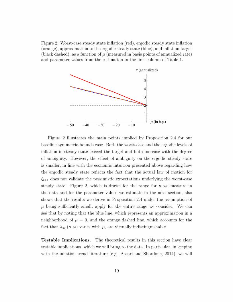
Figure 2: Worst-case steady state inflation (red), ergodic steady state inflation(orange), approximation to the ergodic steady state (blue), and inflation target(black dashed), as a function of µ (measured in basis points of annualized rate)and parameter values from the estimation in the first column of Table 1.

-50 -40 -30 -20 -10Μ Hin b.p.L

1

2

3

4

5

Π HannualizedL

Figure 2 illustrates the main points implied by Proposition 2.4 for our

baseline symmetric-bounds case. Both the worst-case and the ergodic levels of

inflation in steady state exceed the target and both increase with the degree

of ambiguity. However, the effect of ambiguity on the ergodic steady state

is smaller, in line with the economic intuition presented above regarding how

the ergodic steady state reflects the fact that the actual law of motion for

ζt+1 does not validate the pessimistic expectations underlying the worst-case

steady state. Figure 2, which is drawn for the range for µ we measure in

the data and for the parameter values we estimate in the next section, also

shows that the results we derive in Proposition 2.4 under the assumption of

µ being sufficiently small, apply for the entire range we consider. We can

see that by noting that the blue line, which represents an approximation in a

neighborhood of µ = 0, and the orange dashed line, which accounts for the

fact that λπζ (µ, ω) varies with µ, are virtually indistinguishable.

Testable Implications. The theoretical results in this section have clear

testable implications, which we will bring to the data. In particular, in keeping

with the inflation trend literature (e.g. Ascari and Sbordone, 2014), we will

19

give to our model an anticipated utility interpretation and test the following

implications of our model. When the level of ambiguity that minimizes welfare

is µ (µ)

i. both the worst-case steady-state inflation, which maps into our data on

long-run inflation expectations, and the ergodic steady state inflation,

which corresponds to statistical measures of trend inflation, are above

(below) target;

ii. statistical measures of trend inflation should lie between long-run inflation

expectations and the target;

iii. as the degree of ambiguity falls, all measures should tend to converge to

the inflation target.

3 Trend Inflation and Long-run Inflation Ex-

pectations

In order to capture long-run inflation dynamics, Del Negro and Eusepi (2011)

and Del Negro, Giannoni and Schofheide (2015) propose replacing the con-

stant inflation target with a very persistent, exogenous, inflation target pro-

cess. This assumption is very effective at matching inflation data, but seems

at odds with evidence from sources such as the Blue Book – a document il-

lustrating monetary policy alternatives, presented to the FOMC by Fed staff

before each meeting. While the Federal Reserve officially did not have an

explicit numerical target for inflation until 2012, Blue Book simulations have

been produced assuming targets of 1.5% and 2% since at least 2000. Indeed,

Lindsey (2003) states that, as early as July 1996, numerous FOMC committee

members had indicated at least an informal preference for an inflation rate in

the neighborhood of 2%, as indicated by FOMC transcripts of the July 2-3,

1996.

Recently, Carvalho et al. (2017) proposed a model of inflation in which

changes in long-run inflation beliefs are a state-contingent function of short-

run inflation surprises. Their model predicts observed measures of long-term

20

inflation expectations, but cannot account for the observed wedge between

the inflation trend and inflation expectations, because, as in most models, the

inflation trend and long-run survey expectations coincide. However, Chan,

Clark and Koop (2017) present evidence that these two quantities should not

simply be equated; their relationship is more complicated and time-varying.

By introducing ambiguity in our simple New-Keynesian model, we can

make progress in the quest for explaining why long-run inflation expectations

do not correspond to measures of inflation trend, and both differ from the in-

flation target. From the perspective of our model, long-run inflation expecta-

tions would naturally correspond to the worst-case steady state inflation level.

However, an econometrician working with realized inflation would estimate

inflation to settle around a different value in the long run, which corresponds

to the ergodic steady state.13

So, our model allows us to extend the analysis in Sbordone and Ascari

(2014) and Cogley and Sbordone (2008) that studied inflation trend as a time-

varying inflation steady state, as it allows us to study inflation trend and

long-run inflation expectations as separate but related variables.

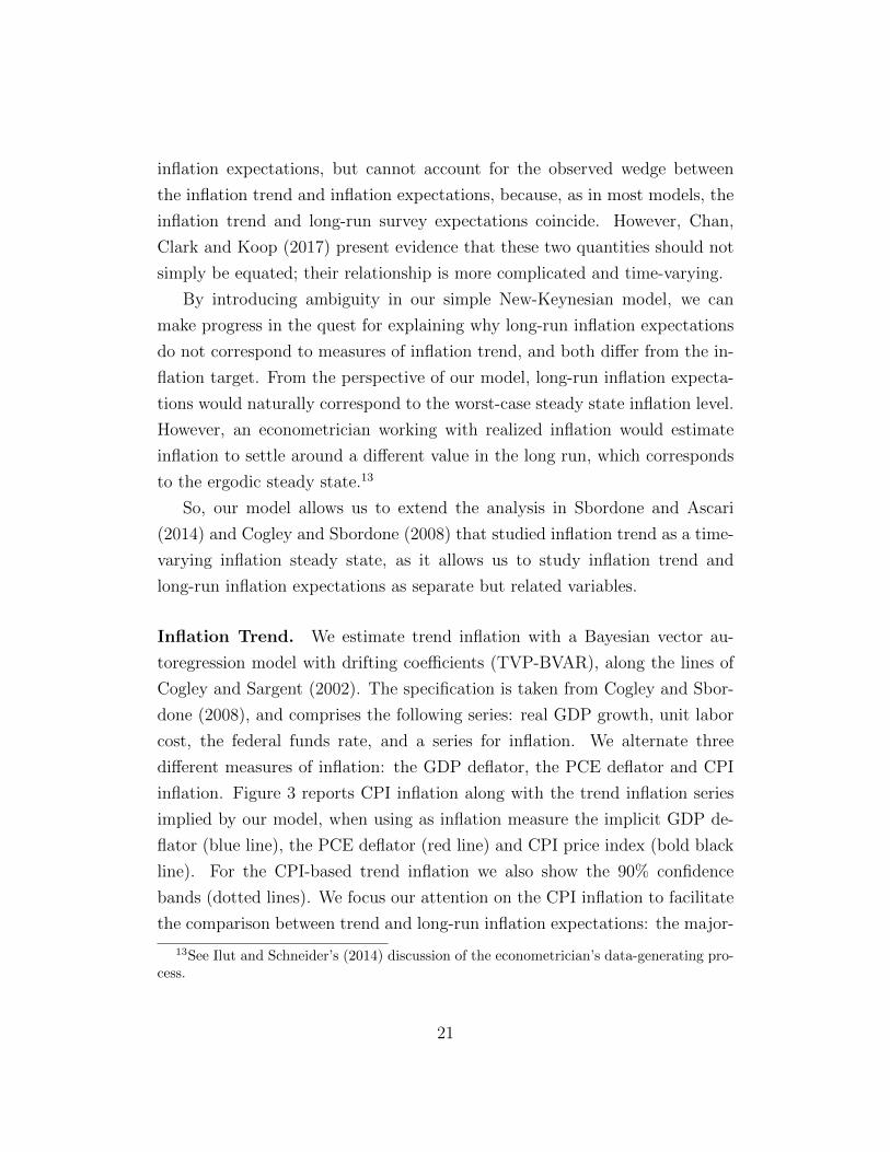
Inflation Trend. We estimate trend inflation with a Bayesian vector au-

toregression model with drifting coefficients (TVP-BVAR), along the lines of

Cogley and Sargent (2002). The specification is taken from Cogley and Sbor-

done (2008), and comprises the following series: real GDP growth, unit labor

cost, the federal funds rate, and a series for inflation. We alternate three

different measures of inflation: the GDP deflator, the PCE deflator and CPI

inflation. Figure 3 reports CPI inflation along with the trend inflation series

implied by our model, when using as inflation measure the implicit GDP de-

flator (blue line), the PCE deflator (red line) and CPI price index (bold black

line). For the CPI-based trend inflation we also show the 90% confidence

bands (dotted lines). We focus our attention on the CPI inflation to facilitate

the comparison between trend and long-run inflation expectations: the major-

13See Ilut and Schneider’s (2014) discussion of the econometrician’s data-generating pro-cess.

21

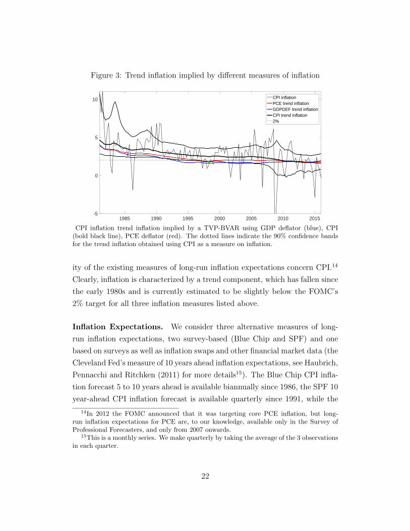
Figure 3: Trend inflation implied by different measures of inflation

1985 1990 1995 2000 2005 2010 2015-5

0

5

10 CPI inflationPCE trend inflationGDPDEF trend inflationCPI trend inflation2%

CPI inflation trend inflation implied by a TVP-BVAR using GDP deflator (blue), CPI(bold black line), PCE deflator (red). The dotted lines indicate the 90% confidence bandsfor the trend inflation obtained using CPI as a measure on inflation.

ity of the existing measures of long-run inflation expectations concern CPI.14

Clearly, inflation is characterized by a trend component, which has fallen since

the early 1980s and is currently estimated to be slightly below the FOMC’s

2% target for all three inflation measures listed above.

Inflation Expectations. We consider three alternative measures of long-

run inflation expectations, two survey-based (Blue Chip and SPF) and one

based on surveys as well as inflation swaps and other financial market data (the

Cleveland Fed’s measure of 10 years ahead inflation expectations, see Haubrich,

Pennacchi and Ritchken (2011) for more details15). The Blue Chip CPI infla-

tion forecast 5 to 10 years ahead is available biannually since 1986, the SPF 10

year-ahead CPI inflation forecast is available quarterly since 1991, while the

14In 2012 the FOMC announced that it was targeting core PCE inflation, but long-run inflation expectations for PCE are, to our knowledge, available only in the Survey ofProfessional Forecasters, and only from 2007 onwards.

15This is a monthly series. We make quarterly by taking the average of the 3 observationsin each quarter.

22

Cleveland Fed produces estimates of inflation expectations at a monthly fre-

quency starting from 1982. We will focus on the Cleveland Fed’s and the Blue

Chip expectations, mainly because of the longer sample, but we will present

the results for SPF expectations as well.

Figure 4 reports these three measures of long-run inflation expectations

and compares them with the measure of trend we obtained with the TVP-

BVAR. Inflation expectations exceed our measure of trend inflation through

the early 2000s. In the aftermath of the Great Recession our preferred measure

of inflation clearly falls below target and also below our declining measure of

trend inflation. The survey-based measures of inflation expectations fall much

less and remain above the 2 percent mark. We attribute the more evident fall

in the Cleveland Fed’s measure of inflation expectation to it including financial

variables. However, it is also important to keep in mind that the 2 percent

target is defined in terms of PCE inflation. CPI inflation has been on average

.4 percentage points higher than PCE inflation over the last 20 years (see for

example Bullard, 2013) as is also evident from our estimates for trend inflation

trend in Figure 3. Taken literally, that would mean that expectations of CPI

below 2.4 percent could be interpreted as below-target expectations.

Ambiguity. We follow Ilut and Schneider (2014) and use disagreement in

survey nowcasts for the Fed Funds rate as our measure of ambiguity. Both

Swanson (2006) and Ehrmann, Eijffinger and Fratzscher (2012) present evi-

dence of a clear link between an increase in central bank transparency in the

1990s and 2000s and a decrease in forecasters’ disagreement about the policy

rate.

Our headline measure of ambiguity about the conduct of monetary policy

is the interdecile dispersion in nowcasts of the current quarter’s federal funds

rate from the Blue Chip Financial Forecasts dataset, which are available from

1983 onwards.

The Blue Chip nowcasts of the federal funds rate are collected on a monthly

basis. Since we want to isolate the uncertainty relating to monetary policy,

rather than macro uncertainty in general, we compare the Blue Chip release

23

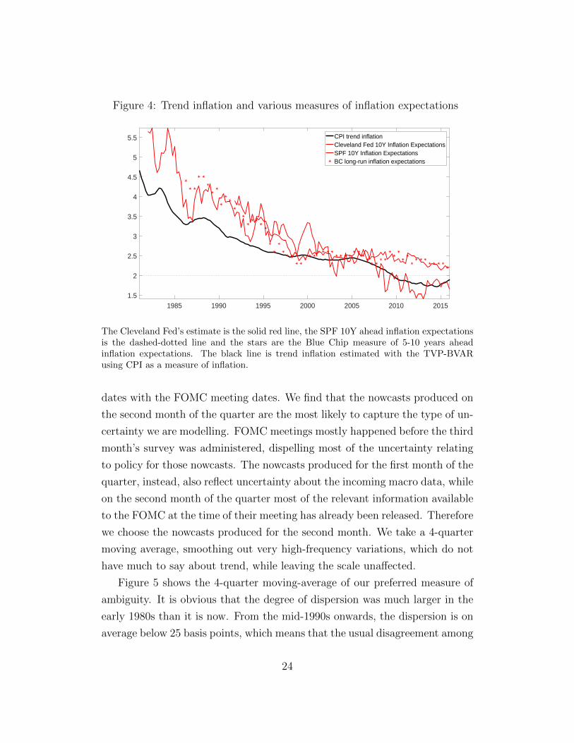
Figure 4: Trend inflation and various measures of inflation expectations

1985 1990 1995 2000 2005 2010 20151.5

2

2.5

3

3.5

4

4.5

5

5.5 CPI trend inflationCleveland Fed 10Y Inflation ExpectationsSPF 10Y Inflation ExpectationsBC long-run inflation expectations

The Cleveland Fed’s estimate is the solid red line, the SPF 10Y ahead inflation expectationsis the dashed-dotted line and the stars are the Blue Chip measure of 5-10 years aheadinflation expectations. The black line is trend inflation estimated with the TVP-BVARusing CPI as a measure of inflation.

dates with the FOMC meeting dates. We find that the nowcasts produced on

the second month of the quarter are the most likely to capture the type of un-

certainty we are modelling. FOMC meetings mostly happened before the third

month’s survey was administered, dispelling most of the uncertainty relating

to policy for those nowcasts. The nowcasts produced for the first month of the

quarter, instead, also reflect uncertainty about the incoming macro data, while

on the second month of the quarter most of the relevant information available

to the FOMC at the time of their meeting has already been released. Therefore

we choose the nowcasts produced for the second month. We take a 4-quarter

moving average, smoothing out very high-frequency variations, which do not

have much to say about trend, while leaving the scale unaffected.

Figure 5 shows the 4-quarter moving-average of our preferred measure of

ambiguity. It is obvious that the degree of dispersion was much larger in the

early 1980s than it is now. From the mid-1990s onwards, the dispersion is on

average below 25 basis points, which means that the usual disagreement among

24

Figure 5: A measure of disagreement about the federal funds rate

1985 1990 1995 2000 2005 2010 20150

0.1

0.2

0.3

0.4

0.5

0.6

0.7

0.8

Annu

aliz

ed P

erce

ntag

e Po

ints

The solid line is the interdecile dispersion of Blue Chip nowcasts of the federal funds ratein the second month of the quarter.

the hawkish and dovish ends of the professional forecasters’ pool amounts to

situations like the former expecting a 25bp tightening and the latter no change

– a very reasonable scenario in the late 1990s and early 2000s. In the early

80s, however, that number exceeded three quarters of a percent.

The implications of our model depend crucially on whether we can think

of the interval [µt, µt] as being symmetric or not. If the interval is symmetric

we can simply calibrate µt to half our measure of dispersion and µt

= −µt.To verify this is a sensible assumption, we test for the symmetry in the dis-

persion of short-term rate nowcasts using a test developed by Premaratne and

Bera (2015).16 Figure 6 shows that the null of symmetry of the distribution

of individual Blue Chip nowcasts of the federal funds rate is only occasion-

ally rejected, and never for several subsequent quarters, up to 2010.17 After

2010/2011, however, the dispersion started to display a noticeable and per-

16This test adjusts the standard√b1 test of symmetry of a distribution, which assumes

no excess kurtosis, for possible distributional misspecifications.17We perform the test on the cross-section of nowcasts at each date in our sample.

25

Figure 6: Test for the null that the distribution of the individual Blue Chipnowcasts is symmetric.

1985 1990 1995 2000 2005 2010 20150

2

4

6

8

10

12

14

16

18

20

skewness statisticα = 1%

We test for the symmetry of the distribution of the individual Blue Chip nowcasts of thefederal funds rate. We use the Premaratne and Bera (2015) test for symmetry of thedistribution and perform it period per period from 1983 to 2015. The test is χ2-distributed.The points above the black line are those in which the null of symmetry is rejected with99% confidence.

sistent upward skew and this determines a persistent rejection of the null

hypothesis of symmetry. Indeed, it is plausible that, the ZLB on policy rates

limits disagreement on the downside precisely in this fashion. In these situa-

tions it is natural that agents would expect the worst-case scenario to be one

in which rates are too high, resulting in a low level of inflation, as our theory

predicts.

3.1 Estimation

Our measures of long-run inflation expectations and inflation trend are highly

correlated (the sample correlation coefficient being .95) and are both negatively

correlated with our measure of ambiguity (sample correlation of -.88 and -.91

for long-run inflation expectations and trend respectively).

26

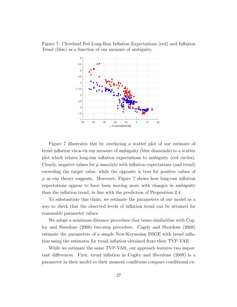
Figure 7: Cleveland Fed Long-Run Inflation Expectations (red) and InflationTrend (blue) as a function of our measure of ambiguity.

-50 -40 -30 -20 -10 0 10 20

µ in annualized bp

1

1.5

2

2.5

3

3.5

4

4.5

5

5.5

6

π

Figure 7 illustrates this by overlaying a scatter plot of our estimate of

trend inflation vis-a-vis our measure of ambiguity (blue diamonds) to a scatter

plot which relates long-run inflation expectations to ambiguity (red circles).

Clearly, negative values for µ associate with inflation expectations (and trend)

exceeding the target value, while the opposite is true for positive values of

µ as our theory suggests. Moreover, Figure 7 shows how long-run inflation

expectations appear to have been moving more with changes in ambiguity

than the inflation trend, in line with the prediction of Proposition 2.4.

To substantiate this claim, we estimate the parameters of our model as a

way to check that the observed levels of inflation trend can be attained for

reasonable parameter values.

We adopt a minimum-distance procedure that bears similarities with Cog-

ley and Sbordone (2008) two-step procedure. Cogely and Sbordone (2008)

estimate the parameters of a simple New-Keynesian DSGE with trend infla-

tion using the estimates for trend inflation obtained from their TVP-VAR.

While we estimate the same TVP-VAR, our approach features two impor-

tant differences. First, trend inflation in Cogley and Sbordone (2008) is a

parameter in their model so their moment conditions compare conditional ex-

27

pectations in the model and in the VAR and the relationship between inflation

and marginal cost. In our case, however, because trend inflation is not exoge-

nous but a function of the level of ambiguity and model parameters, we can

directly minimize the distance between the VAR estimate for trend inflation

and the model-implied measure.

The second difference is that our model provides separate restrictions for

long-run inflation expectations and trend inflation so we can use both to esti-

mate our parameter values.

In particular, we can define our data as zt =[zµt , z

πe

t , ztrendt

]′, t = 1, ..., T

as including a measure of ambiguity18, a measure of long-run inflation expec-

tations and a measure of inflation trend.

We can then use the restrictions from our model to define:

mt (ω, zt) =

zπe

t −(π∗ − zµt

(1−ρζ)(φ−1)

)ztrendt −

(π∗ − zµt

1−ρζ

(1

φ−1+ λπζ (zµt , ω)

)) (20)

so that we can estimate ω by solving the following minimization:

minω∈Ω0

T∑t=1

mt (ω, zt)′Wmt (ω, zt) (21)

where we use the identity matrix as a weighting matrix W in our baseline

estimation. The admissible set Ω0 reflects a number of considerations. First,

our restrictions have nothing to say about ρa so we do not estimate it at all.

In keeping with most empirical macroeconomic literature, we simply calibrate

β = .995. More interestingly, we face two identification challenges. Firstly, it

is very difficult to separately identify θ and ε. These two parameters enter our

moment restrictions via λπζ (zµt , ω) and they both tend to magnify the effects

of steady state inflation,19 so we calibrate ε = 11 – which implies firms price

18We define zµt based on disagreement and the test for symmetry of the interval asdescribed above.

19The definitions of the log-linear coefficients in Appendix C show that the expressionθΠ (µ, ω)

εis recurring. So when Π (µ, ω) > 1, as is the case for most of our sample obser-

vations, ε and θ have similar effects in that they both increase θΠ (µ, ω)ε, which, in turn,

28

their goods at a ten percent markup over their marginal cost – and estimate

θ.

Moreover, lower ρζ and higher φ produce the same effect on the worst-case

steady state level of inflation (our first model condition) and similar effects

on the level of trend inflation – their values impact λπζ (zµt , ω) differently. As

a result in our baseline estimation we set φ = 1.5 (as advocated by Taylor

(1993)) and focus on estimating ρζ . We report the estimation results in which

we estimate both φ and ρζ in Appendix D.1– while the parameter estimates

show more variation when we experiment with different series for long-run

inflation expectations, they are all well within the acceptable range.20

Lastly, imposing that ω ∈ Ω0 ensures that the steady state is well defined

(see equation (16)).21

Table 1 reports our baseline estimates for three different series for inflation

expectations (zπe

t ). The estimates for θ are between .5 and .6, roughly in line

with estimates by Cogely and Sbordone (2008) and Christiano, Eichenbaum

and Evans (2005) who estimate the corresponding parameter with limited-

information techniques at .588 and .60 respectively in different setups and not

far from the .65 estimate in Smets and Wouters (2007). ρζ is estimated to be

around .7, not far from estimates of the autocorrelation term in the monetary

policy rule22 in Smets and Wouters (2007) and Clarida, Galı and Gertler (1999)

which estimate it at .81 and .79 respectively.

We find these results encouraging, since the moments we are matching up

to are not normally used in the estimation of DSGEs. And importantly, from

affects the value of the κ coefficients that enter the definition of λπζ (µ, ω) in equation (19).20In our estimations we set the inflation target π∗ to 2%, the value announced by the

FOMC in 2012 for PCE. This implies a rather conservative value for CPI inflation, whichhas been on average .4 points above PCE inflation in the last 20 years (see for exampleBullard, 2013).

21In practice, we run an unconstrained minimization and then verify that the inequalityin equation (16) is satisfied given the estimates.

22The autocorrelation is most normally modeled as the coefficient on the lagged interestrate. For tractability purposes, we elect to adopt this specification instead, which allows usto keep the derivation analytical as discussed above.

29

Table 1:Cleveland Fed 10Y Blue Chip 5-10Y SPF 10Y

θ 0.5275 0.5834 0.5231ρζ 0.7335 0.7395 0.6962

No of obs. 129 60 97Sample period 1983Q1-2015Q4 1986H1-2015H2 1991Q4-2015Q4

Estimates of θ and ρζ obtained using different measures of long-run inflation expectations

our perspective, our estimates imply that about half of the overall variance of

ζt+1 can be traced back to the predictable component (ρζ2 ≈ .5) and half to

the innovation uζt+1, which seems reasonable given that our dispersion measure

is collected midway through the quarter, in particular between the two FOMC

meetings usually taking place in each quarter.

Figure 8 illustrates the fit of our model and estimation exercise by combin-

ing the data (Figure 7) and the model-implied values (Figure 2).23 This simple

scatter plot confirms our intuition that augmenting a simple New-Keynesian

DSGE with ambiguity regarding the monetary policy rule can go a long way

towards explaining why away from the ZLB inflation expecations tend to ex-

ceed both the target and an estimated trend, with the difference increasing

with the degree of Knightian uncertainty. In the proximity of the lower bound

on policy rates the opposite ranking applies.

The fit is overall better for the inflation trend series than for the inflation

expectations which, in part, is a mechanical consequence of the fact that our

model implies that, of the parameters we estimate, only ρζ can affect the model

counterpart to long-run inflation expectations while both ρζ and θ can make

the model fit the trend series.

In sum, we find that a very simple mininum-distance estimation exercise

of our tightly parametrized model-implied long-run inflation expectations and

inflation trend concepts can do a good job at explaining why with the observed

reduction in our measure of Knightian uncertainty the differences between

long-run expectations and trend fell and both approached the target, only to

23The blue line in Figure 8 corresponds to the blue line in Figure 2, i.e. it uses theapproximation for µ clos to zero. The estimation uses the exact formulation for λπζ (µ, ω)but, as shown above in Figure 2 the two are indistinguishable.

30

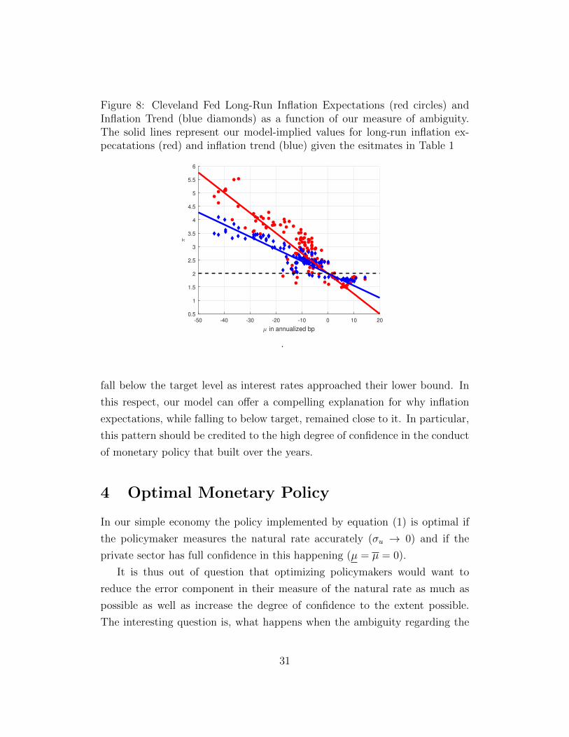
Figure 8: Cleveland Fed Long-Run Inflation Expectations (red circles) andInflation Trend (blue diamonds) as a function of our measure of ambiguity.The solid lines represent our model-implied values for long-run inflation ex-pecatations (red) and inflation trend (blue) given the esitmates in Table 1

-50 -40 -30 -20 -10 0 10 20

µ in annualized bp

0.5

1

1.5

2

2.5

3

3.5

4

4.5

5

5.5

6

π

.

fall below the target level as interest rates approached their lower bound. In

this respect, our model can offer a compelling explanation for why inflation

expectations, while falling to below target, remained close to it. In particular,

this pattern should be credited to the high degree of confidence in the conduct

of monetary policy that built over the years.

4 Optimal Monetary Policy

In our simple economy the policy implemented by equation (1) is optimal if

the policymaker measures the natural rate accurately (σu → 0) and if the

private sector has full confidence in this happening (µ = µ = 0).

It is thus out of question that optimizing policymakers would want to

reduce the error component in their measure of the natural rate as much as

possible as well as increase the degree of confidence to the extent possible.

The interesting question is, what happens when the ambiguity regarding the

31

policy rule cannot be totally dispelled. Here we explore optimal rules for this

scenario.

Our results characterize policy rules that attain the best of possible worst-

case steady-state welfare levels - a concept we will refer to as steady-state

optimality. Steady-state optimality is very often disregarded in analysis of

optimal policy set-ups because, in the absence of ambiguity, zero inflation

and the optimal subsidy deliver the first-best allocation, independent of the

values the other parameters. We will show how, in our setting, the degree of

policy responsiveness to deviations of inflation from target plays a critical role

instead.

We characterize the optimal monetary policy rule when there is a bound on

the responsiveness of the policy rate to inflation. As can be seen in equation

(17), as φ → ∞, steady state approaches first best. However, as Schmitt-

Grohe and Uribe (2007) point out, values of φ above around 3 are impractical.

Hence, we will work under the assumption that values of φ are bounded.

Proposition 4.1. For any ω ∈ Ω, a small µ > 0, µ = −µ and φ ≤ φ ≤ φ,

the following rule is steady-state optimal in its class:

Rt = R∗tΠφt (22)

where R∗t = Rnt e

δ∗(µ,φ;ω) and 0 < δ∗(µ, φ;ω) < µ1−ρζ .

Proof. See Appendix E.2

We can summarize the result by saying that the central bank needs to

be more hawkish than in the abscence of ambiguity, because it is optimal to

respond as strongly as possible to inflation and to increase the monetary policy

rule’s intercept. The overly tight policy stance that Chairman Volcker followed

in early 1982 (see Goodfriend 2005, p. 248) can be better appreciated from

the perspective of this result. In an economy in which ambiguity about policy

was rampant, it was optimal to tighten above and beyond what the business

cycle conditions would seem to dictate.

32

Both high φ and positive δ reduce the wedge between steady-state inflation

and the target, thus increasing welfare. The slope coefficient φ reduces the

effects of ambiguity on inflation because, even if the worst-case interest rate

tends to drive inflation up, this effect is mitigated by a more forceful response

by the policymaker to any deviation from target.

The optimal intercept (R∗t ) is higher than the natural rate, because, as

inflation is still inefficiently high in the presence of ambiguity, the central

bank would like to tighten more. Facing a bound on φ, it can do so only by

increasing the intercept of its policy rule. However, increasing it too much

can be detrimental. On average, the private sector is underestimating the

policy rate by ζ = µ1−ρζ . A naıve policymaker could respond by systematically

setting rates higher than its standard policy rule by the same amount (ζ). If

agents did not evaluate welfare in the worst-case scenario when they make

their decisions, this policy action would implement first best. In our setting,

however, ambiguity-averse agents would realize that the worst-case scenario

had become one in which interest rates are too high and steady state inflation

would end up falling below target. The level of δ that maximizes worst-case

welfare is positive but strictly smaller than µ1−ρζ , capturing the idea that the

policymaker can do better than blindly following the policy rule that would be

optimal in the absence of ambiguity, yet he or she has to prevent the degree of

extra-tightening (δ > 0) to become so large as to make agents fear excessive

tightening more than excessive loosening.

Another important aspect of Proposition 4.1 is that the rule in equation

(22) is optimal in its class, i.e. the class of rules including inflation and a

measure of the natural rate. Clearly, plenty of alternative specifications could

legitimately be proposed. It is not in the spirit of this paper to try to review

and numerically evaluate a great number of alternative rules, but it is immedi-

ate to show that our functional form can deliver as high a level of steady-state

welfare as any other policy scheme, provided we are prepared to relax the con-

straint on φ. In other words, our functional form is only potentially restrictive

in terms of practical implementability, because high values of φ can be hard to

33

justify in practice as we mentioned above, but is otherwise as good as any.24

Finally, our previous result applies under the assumption that the interval

over which the ambiguity is defined is symmetric (µ = −µ). When that is not

the case, as in recent years, the policy prescription still features the highest

possible value for φ but a negative value for δ as we formalize in the following

Corollary.

Corollary 4.1. Given the setup in Proposition 4.1 except for the fact that

|µ| << |µ|, so that V(µ, ω

)> V (µ, ω), then

Rt = R∗tΠφt (23)

where R∗t = Rnt e

δ∗(µ,µ,φ,ω) and − µ1−ρζ < δ∗(µ, µ, φ;ω) < 0 is steady-state opti-

mal in its class.

Proof. See Appendix E.3

This corollary highlights the different roles played by φ and δ. Higher

φ always tends to bring inflation closer to target, so it is always optimal to

increase φ as much as possible, irrespective of whether trend inflation is above

or below target. As for the “policy-rule intercept,” however, when the worst-

case level of inflation is below target, it is optimal for R∗t to be smaller than

the natural rate to generate inflationary pressures that would push inflation

up towards its target.

5 Conclusions

We augment a standard New-Keynesian DSGE to study the consequences of

changes in confidence on the success of an inflationary targeting regime. When

ambiguity-averse agents face Knightian uncertainty about the conduct of mon-

etary policy long-run inflation expectations do not correspond to the inflation

targeting. In particular in normal times inflation expectations will exceed the

target, the distance between the two depending on the degree of ambiguity

24See Corollary in Appendix E.1 for a formal statement.

34

and the central bank’s response to inflation deviations from target, while in

the proximity of the ZLB our model predicts long-run inflation expectations

will fall below the inflation target as the worst-case scenario becomes one in

which policy will be too tight.

Our model also can explain why statistical measures of inflation trend tend

to differ from both the target and long-run expectations, usually falling some-

where in between the two of them. From a modeling perspective this follows

from the realized mean level of inflation reflecting the interaction between pes-

simistic expectations and the fact that the worst-case expectations about the

policy rate do not actually materialize.

By keeping the solution of the model analytical we can easily estimate the

key parameters governing inflation using disagreement on the policy rate as

a measure of ambiguity, long-run inflation expectations from surveys and a

TVP-BVAR estimate for the inflation trend. Our simple minimum distance

procedure is able to fit US trend and inflation expectations data since the early

80’s reasonably well, especially considering how tight the parametrization is –

in our baseline estimation we only estimate two parameters.

Our results are consistent with the idea that the increased level of trans-

parency can explain the transition from a situation in which long-run inflation

expectations exceeded 5 percent in the early 80s to one in which they are

remarkably well anchored around the target – the post Great Recession fall

is much smaller in magnitude relative to the deviations observed in the early

part of our sample, a testament to the much improved degree of anchoring.

We conclude our analysis but characterizing the optimal policy rule in an

ambiguity-ridden economy. In particular, we show how in the presence of

ambiguity a simple monetary policy rule that tracks movements in the natural

rate of interest can be improved upon by one that tracks a higher interest

rate (lower in the vicinity of the ZLB). This provides a novel insight in the

seemingly overly tight policy stance pursued by chairman Volcker in the early

1980s and the ultra low rates observed in the aftermath of the Great Recession.

In sum, by building on the latest advances in the inflation trend literature

(Ascari and Sbordone, 2014) and in the ambiguity literature (Ilut and Schnei-

35

der, 2014) we can provide an economic rationale for observed low-frequency

variations in inflation and inflation expectations which are normally treated

as purely exogenous if not disregarded altogether.

36

References

[1] Ascari, G. and T. Ropele, 2007. “Optimal monetary policy under low

trend inflation,” Journal of Monetary Economics, Elsevier, vol. 54(8),

2568-2583.

[2] Ascari, G. and T. Ropele, 2009. “Trend Inflation, Taylor Principle, and

Indeterminacy,” Journal of Money, Credit and Banking, vol. 41(8), 1557-

1584.

[3] Ascari, G. and A. Sbordone, 2014. “The Macroeconomics of Trend Infla-

tion,” Journal of Economic Literature, vol. 52(3), 679-739.

[4] Baqaee, D.R., 2015.“Asymmetric Inflation Expectations, Downward

Rigidity of Wages and Asymmetric Business Cycles,” Discussion Papers

1601, Centre for Macroeconomics (CFM).

[5] Benigno, P. and L. Paciello, 2014. “Monetary policy, doubts and asset

prices,” Journal of Monetary Economics, 64(2014), 85-98.

[6] Bernanke B.S., 2007. “Federal Reserve Communications.” Speech at the

Cato Institute 25th Annual Monetary Conference, Washington, D.C.

[7] Blinder, A.S., 1998. Central Banking in Theory and Practice. MIT Press.

[8] Bullard, J. 2013. “President’s Message: CPI vs. PCE Inflation: Choosing

a Standard Measure.” The Regional Economist, July 2013.

[9] Calvo, G. A., 1983. “Staggered prices in a utility-maximizing frame-

work,” Journal of Monetary Economics, Elsevier, vol. 12(3), pages 383-

398, September.

[10] Carvalho, S. Eusepi, E. Moench and B. Preston, 2017. Anchored Inflation

Expectations

[11] Chan, C., T. Clark and G. Koop 2017. “A New Model of Inflation,

Trend Inflation, and Long-Run Inflation Expectations.” Journal of Money,

Credit and Banking (forthcoming).

37

[12] Clarida, R., J. Gali, and M. Gertler, 1999. “The Science of Monetary

Policy: A New Keynesian Perspective.” Journal of Economic Literature,

37(4): 1661-1707.

[13] Christiano, L.J, M. Eichenbaum and C.L. Evans, 2005. “Nominal Rigidi-

ties and the Dynamic Effects of a Shock to Monetary Policy,” Journal of

Political Economy, University of Chicago Press, vol. 113(1), pp. 1-45.

[14] Cogley, T. and T.J. Sargent, 2008. “Anticipated Utility And Rational

Expectations As Approximations Of Bayesian Decision Making,” Inter-

national Economic Review, vol. 49(1), pages 185-221, 02.

[15] Cogley, T. and T.J. Sargent, 2002. “Evolving Post World War II U.S.

Inflation Dynamics.” In NBER Macroeconomics annual 2001, edited by

B.S. Bernanke and K. Rogoff, 331-338, MIT press.

[16] Cogley, T. and A.Sbordone, 2008. “Trend Inflation, Indexation, and In-

flation Persistence in the New Keynesian Phillips Curve.” American Eco-

nomic Review, 98(5):2101-26.

[17] Del Negro, M., M.P. Giannoni and F. Schorfheide, 2015. ”Inflation in the

Great Recession and New Keynesian Models,” American Economic Jour-

nal: Macroeconomics, American Economic Association, vol. 7(1), pages

168-96, January

[18] Del Negro, M. and S. Eusepi, 2011. “Fitting observed inflation expecta-

tions,” Journal of Economic Dynamics and Control, Elsevier, vol. 35(12),

pages 2105-2131.

[19] Ehrmann, M., S. Eijffinger and M. Fratzscher, 2012. “The Role of Central

Bank Transparency for Guiding private Sector Forecasts,” Scandinavian

Journal of Economics, 114(3),1018-1052.

[20] Epstein, L.G. and M. Schneider, 2003. “Recursive multiple-priors,” Jour-

nal of Economic Theory, Elsevier, vol. 113(1), pages 1-31.

[21] Galı, J. 2008. Monetary Policy, Inflation, and the Business Cycle: An In-

troduction to the New Keynesian Framework, Princeton University Press.

38

[22] Gilboa, I. and D. Schmeidler, 1989. “Maxmin expected utility with non-

unique prior,” Journal of Mathematical Economics, Elsevier, vol. 18(2),

pp. 141-153

[23] Goodfriend, M., 2005. “The Monetary Policy Debate Since October 1979:

Lessons for Theory and Practice.” Federal Reserve Bank of St. Louis

Review, March/April 2005, 87(2, Part 2), pp. 243-62.

[24] Hansen, L.P. and T. J. Sargent, 2007. Robustness. Princeton University

Press.

[25] Haubrich, J.G., G. Pennacchi, and P. Ritchken, 2011. “Inflation Expec-

tations, Real Rates, and Risk Premia: Evidence from Inflation Swaps,”

Federal Reserve Bank of Cleveland, Working Paper no. 11-07.

[26] Ilut, C. and M. Schneider, 2014. “Ambiguous Business Cycles,” American

Economic Review, American Economic Association, Vol. 104(8), pp. 2368-

99.

[27] Kreps, D.M., 1998. “Anticipated Utility and Dynamics Choice.” In Fron-

tiers of Research in Economic Theory: The Nancy L. Schwartz Memorial

Lectures 1983-1997, edited by D.P. Jacobs, E. Kalai and M.I. Kamien,

242-74. Cambridge University Press

[28] Lindsey, D.E., 2003. A Modern History of FOMC Communication: 1975-

2002, Board of Governors of the Federal Reserve System.

[29] Premaratne, G. and A.K. Bera, 2015. “Adjusting the tests

for skewness and kurtosis for distributional misspecifications,”

Communications in Statistics – Simulation and Computation,

http://dx.doi.org/10.1080/03610918.2014.988254

[30] Rudebusch, G.D., 2002. “Term structure evidence on interest rate smooth-

ing and monetary policy inertia.” Journal of Monetary Economics, Else-

vier, vol. 49(6), pages 1161-1187.

[31] Schmitt-Grohe, S. and M. Uribe, 2007. “Optimal simple and imple-

mentable monetary and fiscal rules,” Journal of Monetary Economics,

Elsevier, vol. 54(6), pages 1702-1725.

39

[32] Stock, J.H. and M. Watson, 2007. “Why has U.S. Inflation Become Harder

to Forecast?” Journal of Money, Credit and Banking, 39(1).

[33] Swanson, E.T., 2006. “Have Increases in Federal Reserve Transparency

Improved Private Sector Interest Rate Forecasts?,” Journal of Money

Credit and Banking, vol. 38(3), pp. 791-819.

[34] Smets, F. and R. Wouters, 2007. “Shocks and Frictions in US Business

Cycles: A Bayesian DSGE Approach,” The American Economic Review,

97(3): 586-606.

[35] Taylor, J.B., 1993. “Discretion versus Policy Rules in Practice,” Carnegie-

Rochester Conference Series on Public Policy 39: 195214.

[36] Yun, T. 2005. “Optimal Monetary Policy with Relative Price Distor-

tions,”American Economic Review, American Economic Association, vol.

95(1), pages 89-109.

40

Appendix - For Online Publication

A Steady State

Pricing. In our model firms index their prices based on the first-best infla-

tion, which corresponds to the inflation target and is zero in the case presented

in the main body of the paper. Because of ambiguity, however, steady-state

inflation will not be zero and therefore there will be price dispersion in steady

state:

∆(µ, ω) =(1− θ)

(1−θΠ(µ,ω)ε−1

1−θ

) εε−1

1− θΠ(µ, ω)ε(24)

∆ is minimised for Π = 1 - or, equivalently, µ = 0 - and is larger than unity

for any other value of µ. As in Yun (2005), the presence of price dispersion

reduces labour productivity and ultimately welfare.

Hours, Consumption and Welfare. In a steady state with no real growth,

steady-state hours are the following function of µ:

N(µ, ω) =

((1− θΠ(µ, ω)ε−1) (1− βθΠ(µ, ω)ε)

(1− βθΠ(µ, ω)ε−1) (1− θΠ(µ, ω)ε)

) 11+ψ

, (25)

while consumption is:

C(µ, ω) =A

∆(µ, ω)N(µ, ω) (26)

Hence the steady state welfare function takes a very simple form:

V(µ, ω) =1

1− β

(log (C(µ, ω))− N(µ, ω)1+ψ

1 + ψ

). (27)

41

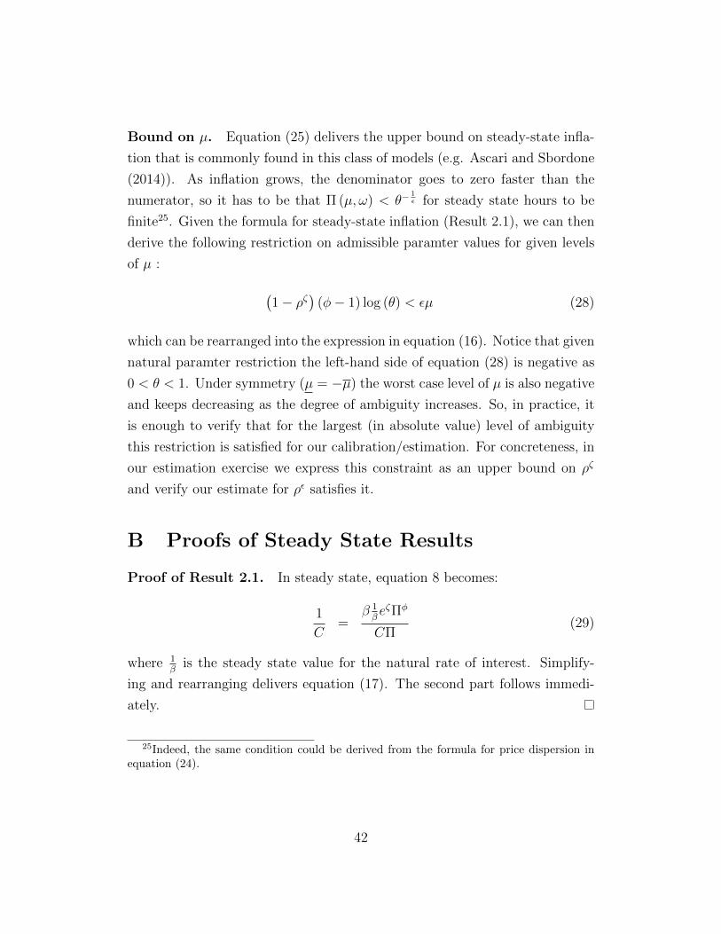
Bound on µ. Equation (25) delivers the upper bound on steady-state infla-

tion that is commonly found in this class of models (e.g. Ascari and Sbordone

(2014)). As inflation grows, the denominator goes to zero faster than the

numerator, so it has to be that Π (µ, ω) < θ−1ε for steady state hours to be

finite25. Given the formula for steady-state inflation (Result 2.1), we can then

derive the following restriction on admissible paramter values for given levels

of µ :

(1− ρζ

)(φ− 1) log (θ) < εµ (28)

which can be rearranged into the expression in equation (16). Notice that given

natural paramter restriction the left-hand side of equation (28) is negative as

0 < θ < 1. Under symmetry (µ = −µ) the worst case level of µ is also negative

and keeps decreasing as the degree of ambiguity increases. So, in practice, it

is enough to verify that for the largest (in absolute value) level of ambiguity

this restriction is satisfied for our calibration/estimation. For concreteness, in

our estimation exercise we express this constraint as an upper bound on ρζ

and verify our estimate for ρε satisfies it.

B Proofs of Steady State Results

Proof of Result 2.1. In steady state, equation 8 becomes:

1

C=

β 1βeζΠφ

CΠ(29)

where 1β

is the steady state value for the natural rate of interest. Simplify-

ing and rearranging delivers equation (17). The second part follows immedi-

ately.

25Indeed, the same condition could be derived from the formula for price dispersion inequation (24).

42

Proof of Proposition 2.2. V (µ, ω), as defined in equation (27), is continu-

ously differentiable around zero. Direct computation, or noting that the first-

best allocation is attained in our model when µ = 0, shows that ∂V(µ,ω)∂µ

= 0.

Direct computation also delivers:

∂2V (µ, ω)

∂µ2

∣∣∣∣µ=0

= − θ ((β − 1)2θ + ε(βθ − 1)2(1 + ψ))

(1− β)(θ − 1)2(βθ − 1)2(φ− 1)2(1 + ψ)(−1 + ρζ)2(30)

All the terms are positive given the minimal theoretical restrictions we impose,

hence the second derivative is strictly negative, which completes the proof of

parts i. and ii..

Direct computation shows that the third derivative evaluated at µ = 0 can be

expressed as:

∂3V (µ, ω)

∂µ3

∣∣∣∣µ=0

=ε(2ε− 1)θ(1 + θ)

(1− β)(1− θ)3(φ− 1)3(1− ρζ)3+R(β) (31)

Where, given our parameter restrictions, the first term on the RHS is positive

andR(β) is a term in β such that limβ→1−R(β) = 0. Hence, limβ→1−∂3V(µ,ω)∂µ3

∣∣∣∣µ=0

=

+∞.

Moreover, ∂

(∂3V(µ,ω)∂µ3

∣∣∣∣µ=0

)/∂β exists, which ensures continuity of the third

derivative in β. Hence the third derivative is positive for any β sufficiently

close to but below unity.

A third-order Taylor expansion around zero can be used to show that, for a

generic small but positive µ0:

V (µ0, ω)− V (−µ0, ω) =∂3V (µ, ω)

∂µ3

∣∣∣∣µ=0

2µ30

6+ o(µ4

0) > 0, (32)

So the steady state value function attains a lower value at −µ0 than it does

at at +µ0. This, combined with the absence of internal minima, delivers our

result under symmetry (µ = −µ).

43

C Model Dynamics

To study the dynamic properties of our model, we log-linearize the equlibrium

conditions around the worst-case steady state. As explained in Ascari and

Ropele (2007), having price dispersion in steady state essentially results in an

additional term in the Phillips Curve. Appendix C.1 presents the log-linear

approximation around a generic steady state indexed by µ. By setting µ = −µ,

we obtain the log-linear approximation to the worst-case steady state (under

symmetry).

Armed with the solution of the log-linearized model, we can verify if the worst-

case indeed corresponds to our conjecture not only in steady state but also

around it.

Once we have verified our conjecture about the worst-case steady state,

we turn our attention to the implications of changes in the agents’ confidence

in their understanding of the monetary policy rule on the determinacy region

and we then study the effects of shocks to ambiguity.

C.1 Log-linearized Equations and Solution

The following equations describe the dynamics of the variables of interest

around a generic steady state indexed by µ26. Setting µ to its worst-case

steady state value, one obtains the log-linear approximation around the worst-

26Where we refer to the numerator of equation (13) as F1 and to the denominator asF2 and express both in recursive form as F1t = ε

ε−1MCt + βθEtΠεt+1F1t+1 and F2t =

1 + βθEtΠε−1t+1F2t+1 respectively.

44

case steady state:

ct = Et [ct+1 − (rt − πt+1)] (33)

πt = κ0 (µ, ω)mct + κ1 (µ, ω)EtF2t+1 + κ2 (µ, ω)Etπt+1 (34)

rt = (rnt + ζt+1) + φπt (35)

∆t = κ3 (µ, ω) ∆t−1 + κ4 (µ, ω) πt (36)

F2t = κ5 (µ, ω)Etπt+1 + κ6 (µ, ω)EtF2t+1 (37)

mct = wt − at (38)

wt = ct + ψnt (39)

yt = at − ∆t + nt (40)

ct = yt (41)

rnt = Etat+1 − at (42)

ynt = at (43)

at = ρaat−1 + uat (44)

45

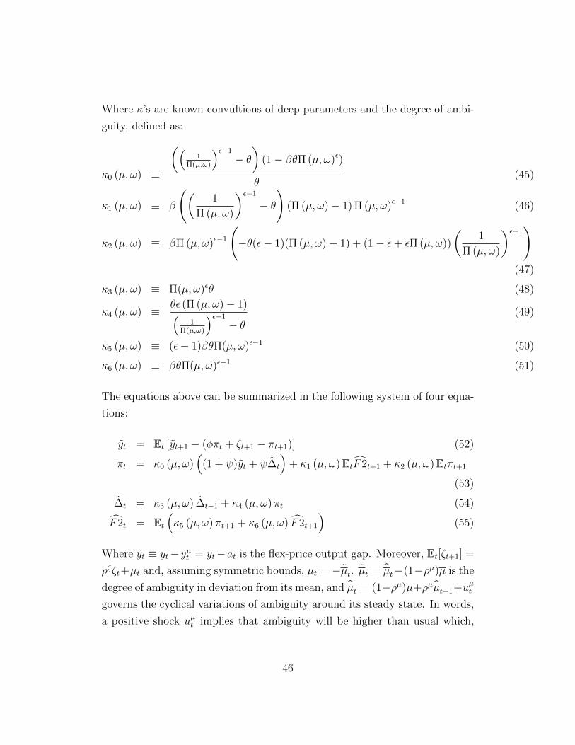
Where κ’s are known convultions of deep parameters and the degree of ambi-

guity, defined as:

κ0 (µ, ω) ≡

((1

Π(µ,ω)

)ε−1

− θ)

(1− βθΠ (µ, ω)ε)

θ(45)

κ1 (µ, ω) ≡ β

((1

Π (µ, ω)

)ε−1

− θ

)(Π (µ, ω)− 1) Π (µ, ω)ε−1 (46)

κ2 (µ, ω) ≡ βΠ (µ, ω)ε−1

(−θ(ε− 1)(Π (µ, ω)− 1) + (1− ε+ εΠ (µ, ω))

(1

Π (µ, ω)

)ε−1)

(47)

κ3 (µ, ω) ≡ Π(µ, ω)εθ (48)

κ4 (µ, ω) ≡ θε (Π (µ, ω)− 1)(1

Π(µ,ω)

)ε−1

− θ(49)

κ5 (µ, ω) ≡ (ε− 1)βθΠ(µ, ω)ε−1 (50)

κ6 (µ, ω) ≡ βθΠ(µ, ω)ε−1 (51)

The equations above can be summarized in the following system of four equa-

tions:

yt = Et [yt+1 − (φπt + ζt+1 − πt+1)] (52)

πt = κ0 (µ, ω)(

(1 + ψ)yt + ψ∆t

)+ κ1 (µ, ω)EtF2t+1 + κ2 (µ, ω)Etπt+1

(53)

∆t = κ3 (µ, ω) ∆t−1 + κ4 (µ, ω) πt (54)

F2t = Et(κ5 (µ, ω) πt+1 + κ6 (µ, ω) F2t+1

)(55)

Where yt ≡ yt−ynt = yt−at is the flex-price output gap. Moreover, Et[ζt+1] =

ρζζt+µt and, assuming symmetric bounds, µt = −µt. µt = µt−(1−ρµ)µ is the

degree of ambiguity in deviation from its mean, and µt = (1−ρµ)µ+ρµµt−1+uµt

governs the cyclical variations of ambiguity around its steady state. In words,

a positive shock uµt implies that ambiguity will be higher than usual which,

46

under our worst-case steady state results27, means that agents will ”increase

their underestimation of the policy rate”.

These equation make it transparent that technological shocks do not affect

any of the four variables in this system and, in particular, the output gap and

inflation. This is common in models in which the natural rate enters the policy

rule but it useful to verify that this property extends to the case in which we

log-linearize the model around the worst-case steady state. at will still play a

role, though, in that consumption, and thus utility, respond to it.

C.2 Worst-Case around the Steady State

We now need to study welfare around the worst-case steady state. To preserve

analytical tractability we focus on the case in which hours enter felicity linearly

(ω ∈ Ω0) and follow a similar approach to that in Ilut and Scheider (2014),

section II. Namely:

i. Based on Result 2.2, we determine the worst-case steady state, i.e. µ =

−µ under symmetry.

ii. We then solve for the linear policy functions, thus getting a mapping from

the state of the economy st = (∆t−1, ζt, at, µt)28 onto all the endogenous

variables of interest, most notably ct and nt, which determine welfare.

iii. We then verify whether welfare is increasing in ζt, consistent with the

guess that the worst-case scenario is that in which its expectation takes

the lower value on the range (−µ).

If hours enter felicity linearly (ψ = 0), the price dispersion term drops out

of equation (53). As a result, while price dispersion still affects hours worked

and thus welfare, it does not enter the policy functions for inflation, the output

gap and the forward-looking term F2t. Moreover, the presence of the natural

27The next section explores how it holds around the worst-case steady state.28Under symmetry, we do not need to keep track of variations in µ and µ separately,

hence the state of the economy is smaller.

47

rate in the policy rule, implies that technology also does not affect any of these

variables (while affecting welfare via consumption and hours). So ultimately

Policy functions for these variables are thus linear functions in (ζt, µt),

where we use λ’s to denote the coefficients, which can be computed analytically

in this case using the method of undetermined coefficients.

For this particular exercise, the only relevant coefficients are those pertain-

ing to ζt so we only report the expressions for them:

πt = λπζζt + λπµµt λπζ ≡−κ0ρ

ζ

(1− ρζ)(

1 + (φ−ρζ)κ01−ρζ − ρζ

(κ2 + ρζκ1κ5

1−ρζκ6

))(56)

yt = λyζζt + λyµµt λyζ ≡ρζ +

(φ− ρζ

)λπζ

1− ρζ(57)

F2t = λFζζt + λFµµt λFζ ≡ρζκ5λπζ1− ρζκ6

(58)

∆t = κ3∆t−1 + κ4

(λπζζt + λπµµt

)(59)

where κ’s are defined in equations (45)-(51).

Using the expressions in Section C.1 we can then out the policy functions for

consumption and hours:

ct = yt + at = λyζζt + +λyµµt + at (60)

nt = ct − at + ∆t = yt + ∆t = λyζζt + λyµµt + κ3∆t−1 + κ4

(λπζζt + λπµµt

)(61)

Turning to the value function, we can express it using the policy functions, as:

V(

∆t−1, ζt, at, µt

)= log ((1 + ct)C(−µ, ω))− (1 + nt)N (−µ, ω) + βEtV

(∆t, ζt+1, at+1, µt+1

)(62)

V(

∆t−1, ζt, at, µt

)= [log (C(−µ, ω))−N (−µ, ω)] + log (1 + ct)− ntN (−µ, ω) + βEtV

(∆t, ζt+1, at+1, µt+1

)(63)

V(

∆t−1, ζt, at, µt

)= u

(−→C (−µ, ω)

)+ log (1 + ct)− ntN (−µ, ω) + βEtV

(∆t, ζt+1, at+1, µt+1

)(64)

48

We can then define dV(

∆t−1, ζt, at, µt

)≡ V

(∆t−1, ζt, at, µt

)− V (−µ, ω),

which can be expressed as:

dV(

∆t−1, ζt, at, µt

)= log (1 + ct)− ntN (−µ, ω) + βEtdV

(∆t, ζt+1, at+1, µt+1

)(65)

dV(

∆t−1, ζt, at, µt

)= ct − nt + βEtdV

(∆t, ζt+1, at+1, µt+1

)(66)

dV(

∆t−1, ζt, at, µt

)= at − ∆t + βEtdV

(∆t, ζt+1, at+1, µt+1

)(67)

dV(

∆t−1, ζt, at, µt

)= at − κ3∆t−1 − κ4λπζζt − κ4λπµµt + βEtdV

(∆t, ζt+1, at+1, µt+1

)(68)

The result29 clearly illustrates how, to a first-order approximation, welfare

around the worst-case steady state moves with the difference between con-

sumption and hours worked (equation (66)) which, in turn can be expressed

as the difference between the level of technology and that of price disper-

sion (equation (67)). This is obvious if one considers the resource constraint:

Ct = At∆tNt. Both At and ∆t act as wedges between the level of consumption

and that of hours, though they work in opposite directions.

Moreover, while At is completely exogenous, ∆t is a discounted sum of past

deviations of inflation from steady state. As demonstrated in Proposition 2.4,

λπζ < 0. On the other hand, κ4 > 0 when Π (µ, ω) > 1, as is the case in the

worst-case steady state under symmetry30.

This means that a lower value for ζt will lead to an increase in inflation

(it is a loosening in the monetary policy stance), which results in an increase

in the price dispersion index for the foreseeable future (κ3 > 0). As a result,

lower ζt will result in a lower level of welfare, which illustrates how welfare

is increasing in ζt, so that a pessimistic agent would act on the assumption

that ζt will be lower in the future. Which is the conjecture we make when we

assume that the expectation distortion µt equals −µt at all times so long as

29We use the Taylor approximation for log(1+ct) and the fact that N (−µ, ω), as definedin (25), is extremely close to one for reasonable values for µ.

30Notice that the condition presented in equation (28) implies that θΠ (µ, ω)ε< 1. When

Π (µ, ω) > 1, θΠ (µ, ω)ε−1

< θΠ (µ, ω)ε< 1 so the condition in equation (28), which we is

necessary for hours worked in steady state to be positive, implies that the denominator ofequation (49) is positive.

49

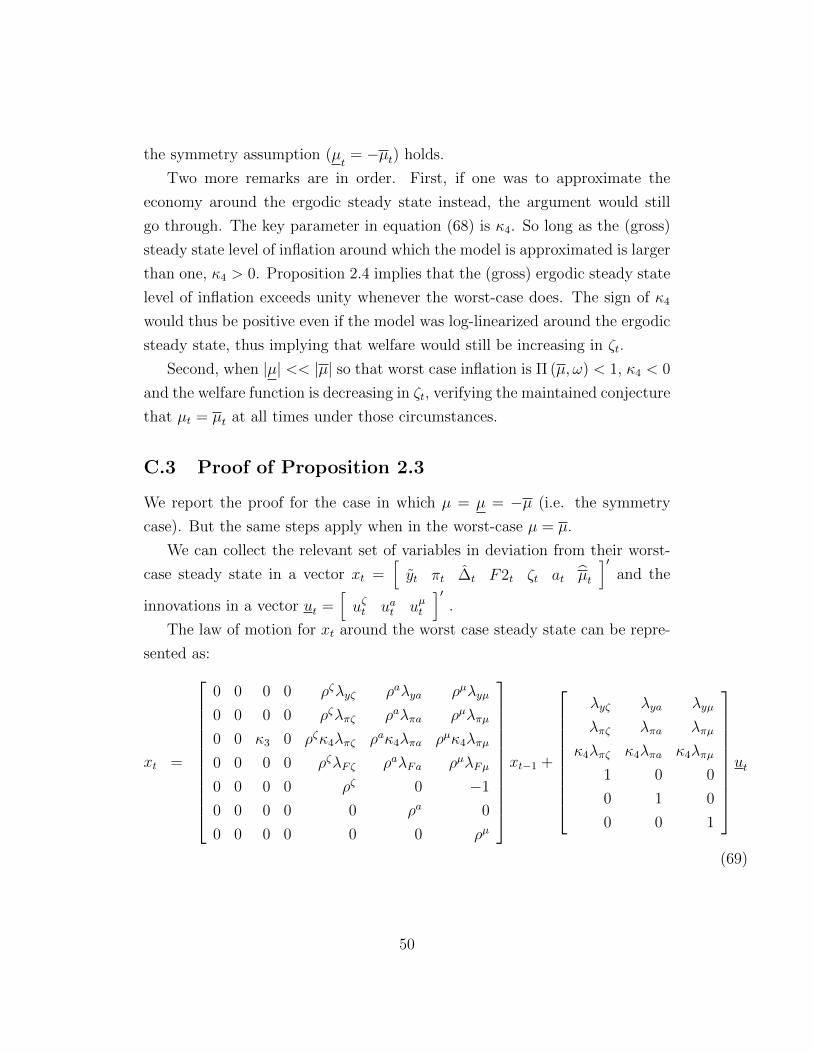
the symmetry assumption (µt

= −µt) holds.

Two more remarks are in order. First, if one was to approximate the

economy around the ergodic steady state instead, the argument would still

go through. The key parameter in equation (68) is κ4. So long as the (gross)

steady state level of inflation around which the model is approximated is larger

than one, κ4 > 0. Proposition 2.4 implies that the (gross) ergodic steady state

level of inflation exceeds unity whenever the worst-case does. The sign of κ4

would thus be positive even if the model was log-linearized around the ergodic

steady state, thus implying that welfare would still be increasing in ζt.

Second, when |µ| << |µ| so that worst case inflation is Π (µ, ω) < 1, κ4 < 0

and the welfare function is decreasing in ζt, verifying the maintained conjecture

that µt = µt at all times under those circumstances.

C.3 Proof of Proposition 2.3

We report the proof for the case in which µ = µ = −µ (i.e. the symmetry

case). But the same steps apply when in the worst-case µ = µ.

We can collect the relevant set of variables in deviation from their worst-

case steady state in a vector xt =[yt πt ∆t F2t ζt at µt

]′and the

innovations in a vector ut =[uζt uat uµt

]′.

The law of motion for xt around the worst case steady state can be repre-

sented as:

xt =

0 0 0 0 ρζλyζ ρaλya ρµλyµ

0 0 0 0 ρζλπζ ρaλπa ρµλπµ

0 0 κ3 0 ρζκ4λπζ ρaκ4λπa ρµκ4λπµ

0 0 0 0 ρζλFζ ρaλFa ρµλFµ

0 0 0 0 ρζ 0 −1

0 0 0 0 0 ρa 0

0 0 0 0 0 0 ρµ

xt−1 +

λyζ λya λyµ

λπζ λπa λπµ

κ4λπζ κ4λπa κ4λπµ

1 0 0

0 1 0

0 0 1

ut

(69)

50

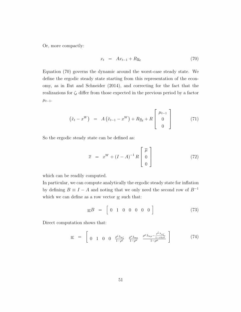
Or, more compactly:

xt = Axt−1 +Rut (70)

Equation (70) governs the dynamic around the worst-case steady state. We

define the ergodic steady state starting from this representation of the econ-

omy, as in Ilut and Schneider (2014), and correcting for the fact that the

realizazions for ζt differ from those expected in the previous period by a factor

µt−1.

(xt − xW

)= A

(xt−1 − xW

)+Rut +R

µt−1

0

0

(71)

So the ergodic steady state can be defined as:

x = xW + (I − A)−1R

µ

0

0

(72)

which can be readily computed.

In particular, we can compute analytically the ergodic steady state for inflation

by defining B ≡ I − A and noting that we only need the second row of B−1

which we can define as a row vector w such that:

wB =[

0 1 0 0 0 0 0]

(73)

Direct computation shows that:

w =

[0 1 0 0

ρζλπζ1−ρζ

ρaλπa1−ρa

ρµλπµ−ρζλπζ

1−rhoζ

1−ρµ

](74)

51

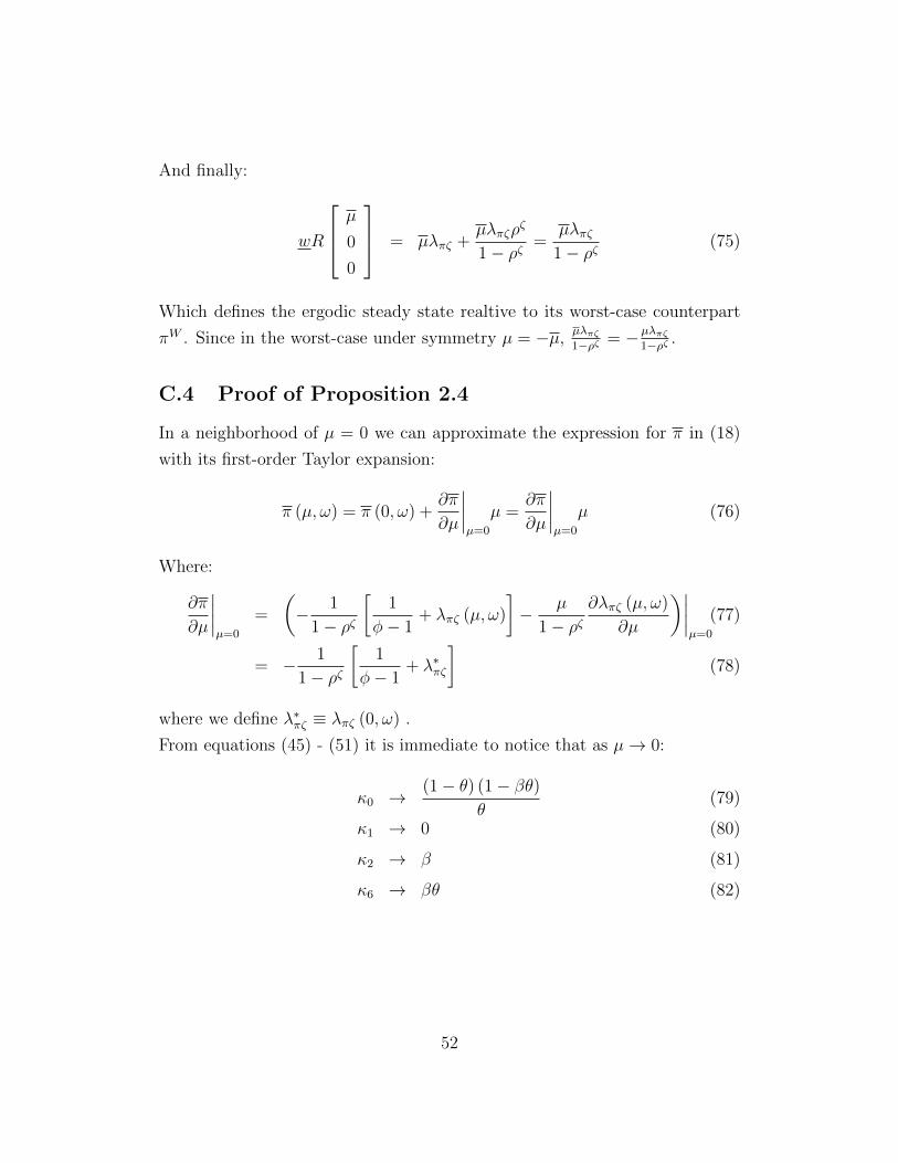
And finally:

wR

µ

0

0

= µλπζ +µλπζρ

ζ

1− ρζ=

µλπζ1− ρζ

(75)

Which defines the ergodic steady state realtive to its worst-case counterpart

πW . Since in the worst-case under symmetry µ = −µ,µλπζ1−ρζ = −µλπζ

1−ρζ .

C.4 Proof of Proposition 2.4

In a neighborhood of µ = 0 we can approximate the expression for π in (18)

with its first-order Taylor expansion:

π (µ, ω) = π (0, ω) +∂π

∂µ

∣∣∣∣µ=0

µ =∂π

∂µ

∣∣∣∣µ=0

µ (76)

Where:

∂π

∂µ

∣∣∣∣µ=0

=

(− 1

1− ρζ

[1

φ− 1+ λπζ (µ, ω)

]− µ

1− ρζ∂λπζ (µ, ω)

∂µ

)∣∣∣∣µ=0

(77)

= − 1

1− ρζ

[1

φ− 1+ λ∗πζ

](78)

where we define λ∗πζ ≡ λπζ (0, ω) .

From equations (45) - (51) it is immediate to notice that as µ→ 0:

κ0 →(1− θ) (1− βθ)

θ(79)

κ1 → 0 (80)

κ2 → β (81)

κ6 → βθ (82)

52

So λ∗πζ = 1

1− φ

ρζ−θ(1−βρζ)(1−ρζ)ρζ(1−βθ)(1−θ)

.

Moreover:

∂λ∗πζ∂θ

=ρζ (1− βθ)

(1− ρζ

) (1− βρζ

)((θ − ρζ) (1− βθρζ)− (1− θ) (1− βθ)φ)2 > 0 ∀ω ∈ Ω0 (83)

∂λ∗πζ∂ρζ

= −(1− θ) (1− βθ)

(θ(1− β(ρζ)2

)+ (1− θ) (1− βθ)φ

)((θ − ρζ) (1− βθρζ)− (1− θ) (1− βθ)φ)2 < 0 ∀ω ∈ Ω0

(84)

∂λ∗πζ∂β

=ρζθ (1− θ)

(1− ρζ

) (θ − ρζ

)((θ − ρζ) (1− βθρζ)− (1− θ) (1− βθ)φ)2 (85)

So λ∗πζ is continuous and monotonic in θ and ρζ . It is also weakly monotonic

in β: increasing if θ > ρζ > 0, flat if θ = ρζ and decreasing otherwise. So we

only need to check the extremes:

λ∗πζ →

− ρζ

φ−ρζ as θ → 0

0 as θ → 1

0 as ρζ → 0

− 1φ−1

as ρζ → 1

(86)

1

1− φρζ− θ(1−ρζ)(1−ρζ)

ρζ(1−θ)(1−θ)

→

− ρζ

φ−ρζ as θ → 0

0 as θ → 1

0 as ρζ → 0

− 1φ−1

as ρζ → 1

(87)

1

1− φρζ− θ(1−ρζ)

ρζ(1−θ)

→

− ρζ

φ−ρζ as θ → 0

0 as θ → 1

0 as ρζ → 0

− 1φ−1

as ρζ → 1

(88)

Where the second and third expressions are the limits for λ∗πζ as β tends to 1

and to 0, respectively.

53

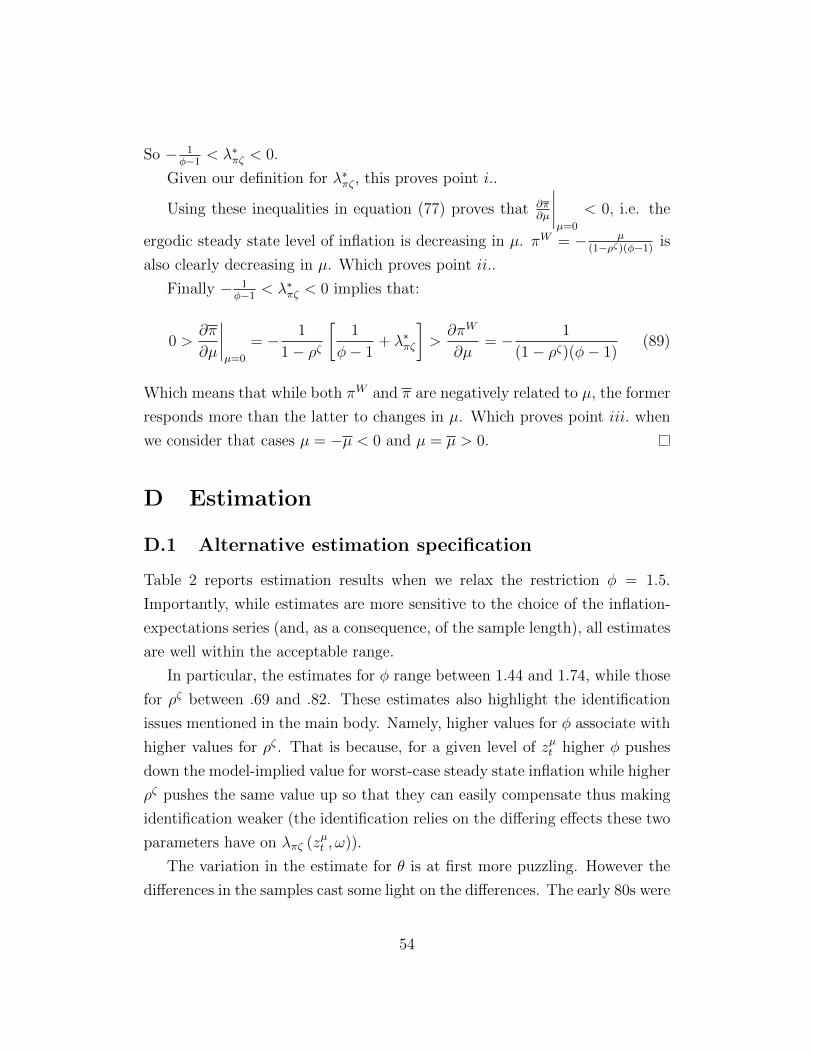
So − 1φ−1

< λ∗πζ < 0.

Given our definition for λ∗πζ , this proves point i..

Using these inequalities in equation (77) proves that ∂π∂µ

∣∣∣∣µ=0

< 0, i.e. the

ergodic steady state level of inflation is decreasing in µ. πW = − µ(1−ρζ)(φ−1)

is

also clearly decreasing in µ. Which proves point ii..

Finally − 1φ−1

< λ∗πζ < 0 implies that:

0 >∂π

∂µ

∣∣∣∣µ=0

= − 1

1− ρζ

[1

φ− 1+ λ∗πζ

]>∂πW

∂µ= − 1

(1− ρζ)(φ− 1)(89)

Which means that while both πW and π are negatively related to µ, the former

responds more than the latter to changes in µ. Which proves point iii. when

we consider that cases µ = −µ < 0 and µ = µ > 0.

D Estimation

D.1 Alternative estimation specification

Table 2 reports estimation results when we relax the restriction φ = 1.5.

Importantly, while estimates are more sensitive to the choice of the inflation-

expectations series (and, as a consequence, of the sample length), all estimates

are well within the acceptable range.

In particular, the estimates for φ range between 1.44 and 1.74, while those

for ρζ between .69 and .82. These estimates also highlight the identification

issues mentioned in the main body. Namely, higher values for φ associate with

higher values for ρζ . That is because, for a given level of zµt higher φ pushes

down the model-implied value for worst-case steady state inflation while higher

ρζ pushes the same value up so that they can easily compensate thus making

identification weaker (the identification relies on the differing effects these two

parameters have on λπζ (zµt , ω)).

The variation in the estimate for θ is at first more puzzling. However the

differences in the samples cast some light on the differences. The early 80s were

54

not only characterized by high inflation expectation and trend but also by a

larger difference between the two series. In our model the difference between

the two series depends primarily by lambdaπζ . To gain some intuition we can

use the formula for λ∗πζ we derived in Appendix 2.4, the level to which λπζ (µ, ω)

converges to as µ → 0, and plug in the estimated values under the different

scenarios. If we use the estimates in Table 2 the implied values for λ∗πζ range

between -.88 (for the Cleveland Fed 10Y inflation expectations series, the series

that goes back to the early 80s) and -.52 (for the SPF 10Y estimation, which

starts in the 90’s). If we consider the estimates, the corresponding values for

λ∗πζ are -.78 and -.68. Restricting the value for φ, trivially, makes it harder to

fit the two series and, as it seems, consequently reduces the effect that different

samples have on the estimates (primarily that of θ).

Since even our more restrictive estimation seem to be fitting the data rea-

sonably well we opt to use that as our baseline.

Table 2:Cleveland Fed 10Y Blue Chip 5-10Y SPF 10Y

φ 1.4372 1.7407 1.6737θ 0.2661 0.7921 0.7462ρζ 0.6950 0.8242 0.7745

No of obs. 129 60 97Sample period 1983Q1-2015Q4 1986H1-2015H2 1991Q4-2015Q4

Estimates of θ and ρζ obtained using different measures of long-run inflation expectations

D.2 Time-Series of the actual and fitted values for trend

inflation and inflation expectations

Figure 9 overlays the measures of trend inflation implied by our model and

our baseline estimate for the CPI inflation trend, along with the Cleveland

Fed’s measure of inflation expectations and the long-run inflation expectations

implied by the model.

As mentioned in the main body of the text, our estimate for long-run

inflation expectations undershoots the outturn for a number of years in the

55

Figure 9: Trend inflation and inflation expectations implied by our measureof disagreement

1985 1990 1995 2000 2005 2010 20151

1.5

2

2.5

3

3.5

4

4.5

5

5.5Cleveland Fed 10Y Ahead Inflation ExpectationsModel-implied Inflation ExpectationsTrend Inflation (TVP-BVAR)Model-implied Trend Inflation

1990s, which is mostly attributable to the fact that our inflation target of 2

percent is defined in terms of PCE inflation, which is on average lower than

CPI inflation.

Also, we can note a short-lived period around the onset of the Great Reces-

sion when our model read the increase in uncertainty as pushing up on inflation

expectations until rates fell to the point when the [µ, µ] became asymmetric

thus changing the direction in which inflation moves in response to an in in-

crease in Knightian uncertainty.

All things considered, though, we find that the model-implied trend in-

flation does a good job at capturing the decline in the secular component of

inflation in the data, the fact that, over recent years, the inflation trend fell

below the 2% mark, while also helping us to make sense of the progressive

reduction of the wedge between inflation expectations and trend inflation.

56

E Optimal Policy

E.1 Useful Lemmas

With a slight abuse of notation we use ω to refer to all parameter values but

φ in the following Lemma and in other similar circumstances in this section

when we want to study the effects of φ while keeping the other parameters

fixed.

Lemma E.1. For any ω ∈ Ω and µ, a small positive number, given any pair

(µ, φ) ∈ [−µ, 0) × (1,∞), for any µ′ ∈ [µ, 0) there exists φ′ ∈ (1, ∞) such

that:

V(µ, φ′, ω) = V(µ′, φ, ω)

And φ′ ≥ φ iff µ′ ≥ µ.

A corresponding equivalence holds for µ ∈ (0, µ].

Proof. Inspection reveals that µ and φ only enter steady-state welfare through

the steady-state inflation term Π(µ, ω) = eµ

(1−φ)(1−ρζ) . It follows immediately

that, for a given µ′, φ′ = 1 + (φ−1)µµ′

implies that (µ, φ′) is welfare equivalent to

(µ′, φ). (µ, µ′) ∈ [µ, 0) × [µ, 0) ensures that µ′ · µ > 0 and so φ′ ∈ (1,∞) for

any φ > 1. The inequalities follow immediately from the definition of φ′ given

above and the fact that both µ and µ′ are both negative.

A similar argument would go through for (µ, µ′) ∈ (0, µ]× (0, µ].

Lemma E.2. Define Vδ (µ, δ, ω) to be the welfare function of an economy

identical to that described in Section 2 except for the fact that the policy rule

has a constant term δ entering as follows:

Rt =(Rnt e

ζt+1eδ)

(Πt)φ (90)

57

Then Vδ (), for a generic value µ, can be expressed as a function of welfare in

the baseline economy for a different value of µ in the following way:

Vδ (µ, δ, ω) = V(µ+ δ, ω

)(91)

where δ ≡(1− ρζ

)δ.

Proof. The computation of the steady state of the model in Section A reveals

that the steady state in this model can be thought of as expressing all the

variables as a function of steady state inflation and steady state inflation as

a function of µ, because µ only enters the model via the steady state level of

inflation. The same is true of δ.

Substituting equation (90) for equation (1) and following the Proof of Result

2.1 yield the following steady state value for inflation:

Π (µ, δ, ω) = e− µ

(φ−1)(1−ρζ)− δφ−1 = e

− µ+δ

(φ−1)(1−ρζ) (92)

This level of steady state inflation (and consequently of welfare) is equivalent

to that in the original economy for a value µ′, where µ′ = µ+ δ.

Lemma E.3. Assuming that V(µ, ω) takes only real values over some interval

(m,m) such that m > µ > 0 > µ > −m, is continuously differentiable, strictly

concave and attains a finite maximum at µ = µ0 ∈ (m,m); then the level of δ

that maximizes worst-case steady-state welfare is implicitly defined as:

δ∗(µ, µ) : V(µ+ δ∗(µ, µ), ω

)= V

(µ+ δ∗(µ, µ), ω

)(93)

Proof. Given Lemma E.2 we can use the welfare function for the original econ-

omy and its properties derived in Proposition 2.2.

First, note that strict concavity ensures µ0 is the unique maximum.

Second, consider the following cases:

1. µ0 ∈ (µ, µ): then V′(µ, ω) > 0 > V′(µ, ω)

58

a. V(µ, ω) < V(µ, ω). Together with strict concavity this implies that

the minimum (or worst-case) over [µ, µ] is µ. Then there exists a

small δ > 0 such that

V(µ, ω) < V(µ+ δ, ω) < V(µ+ δ, ω) < V(µ, ω).

So now the worst case µ+ δ generates a higher level of welfare. The

worst-case welfare can be improved until the second inequality above

holds with equality. Continuity ensures such a level of δ∗ exists. Our

assumptions also ensure that µ0 − µ > δ∗31, because if µ + δ = µ0,

V(µ+ δ) = V(µ0) which is a unique maximum so the equality cannot

hold. This, in turn ensures that V′(µ+ δ∗) > 0 > V′(µ+ δ∗). Hence,

any further increase in δ would make µ+ δ the worst case and welfare

at the worst-case would fall.

b. V(µ, ω) > V(µ, ω). Together with strict concavity, this implies that

the minimum is attained at µ. Then there exists a small enough

δ < 0 such that:

V(µ, ω) < V(µ+ δ, ω) < V(µ+ δ, ω) < V(µ, ω)

By the same arguments as above µ0 − µ < δ∗ < 0 makes the second

inequality hold with equality and attains the higher level of welfare.

c. V(µ, ω) = V(µ, ω). Any δ 6= 0 would lower the worst-case welfare:

δ∗ = 0.

2. µ0 ∈ [µ,m). Strict concavity implies that welfare is strictly increasing

over [µ, µ] and µ mimizes welfare over that range. For all 0 ≤ δ ≤ µ0− µ

V(µ, ω) ≤ V(µ+ δ, ω) < V(µ+ δ, ω) ≤ V(µ0, ω)

The second inequality will always be strict. For δ just above µ0 − µ the

logic of case 1a above applies and δ∗ can be determined accordingly.

31Clearly µ0 − µ > 0, since µ0 > µ in this case.

59

3. µ0 ∈ (m,µ]. Strict concavity implies that welfare is strictly decreasing

over [µ, µ] and µ mimizes welfare over that range. For all 0 ≥ δ ≥ µ0− µ

V(µ0, ω) ≥ V(µ+ δ, ω) > V(µ+ δ, ω) ≥ V(µ, ω)

The second inequality will always be strict. For δ just below µ0 − µ the

logic of case case 1b above applies and δ∗ can be determined accordingly.

E.2 Proof of Proposition 4.1

Lemma E.2 applies so we will use the welfare function of the original economy.

Then, the proof of static optimality proceeds in two steps by first findind the

optimal value of φ given assumptions on the welfare function and on δ and

then verifying that for φ, the conjectures made in the previous point hold.

i. Suppose that V(−µ+ δ, ω) corresponds to the worst-case steady-state wel-

fare for some δ ∈ (0, µ), then φ = φ maximizes worst-case welfare over

[φ, φ].

Following the same logic as in Lemma E.1, but using the expression in

equation (92) for inflation, it is easy to verify that for any 1 < φ′ < φ,

there exists a µ′ s.t.:

V(µ′ + δ, φ′, ω

)= V

(−µ+ δ, φ, ω

)(94)

In particular:

µ′ = −µ(φ′ − 1

φ− 1

)− δ

(1− φ′ − 1

φ− 1

)(95)

Given our parameter restrictions, this implies that 0 > −δ > µ′ > −µ.

In our economy V(0, ω) corresponds to the maximum, so the argmax

µ = −δ. Together with strict concavity (Proposition 2.2), this implies

60

that, in this case, V() strictly increasing for µ < −δ, hence:

V(−µ+ δ, φ, ω

)= V

(µ′ + δ, φ′, ω

)> V

(−µ+ δ, φ′, ω

)(96)

which implies that φ maximizes welfare over [φ, φ] for φ > 1 which we

maintain throughout (equation (16)).

ii. 0 < δ∗ < µ defined by V(−µ+ δ∗, ω

)= V

(µ+ δ∗, ω

)maximizes worst-

case welfare for φ = φ.

Proposition 2.2 guarantees that our welfare function satisfies the assump-

tions of Lemma E.3 in a neighborhood of zero.

To find the bounds on δ∗, note that for µ > 0 and µ = −µ, Propo-

sition 2.2 also implies that the maximum µ0 = 0 is interior and that

V(µ, ω) < V(µ, ω). So, case 1a of the proof of Lemma E.3 applies, which

implies that µ0 − µ = µ > δ∗ > 0. These considerations apply for any

φ > 1, thus also for φ.

E.3 Proof of Corollary 4.1

Following the same approach as for Proposition 4.1

i. Suppose that V(µ + δ, ω) corresponds to the worst-case steady-state wel-

fare for some δ ∈ (−µ, 0), then φ = φ maximizes worst-case welfare over

[φ, φ].

For any 1 < φ′ < φ, there exists a µ′ s.t.:

V(µ′ + δ, φ′, ω

)= V

(µ+ δ, φ, ω

)(97)

In particular:

µ′ = µ

(φ′ − 1

φ− 1

)− δ

(1− φ′ − 1

φ− 1

)(98)

61

Given our restrictions, this implies that 0 < −δ < µ′ < µ.

V() is strictly decreasing for µ > −δ, hence:

V(µ+ δ, φ, ω

)= V

(µ′ + δ, φ′, ω

)> V

(µ+ δ, φ′, ω

)(99)

ii. 0 > δ∗ > −µ defined by V(µ+ δ∗, ω

)= V

(µ+ δ∗, ω

)maximizes worst-

case welfare for φ = φ.

V(µ, ω) > V(µ, ω) and for µ < 0 and µ > 0 the welfare maximum µ0 = 0

is in the interior. This corresponds to case 1b of the proof of Lemma E.3,

which implies that µ0 − µ = −µ < δ∗ < 0.

E.4 Corollary: general applicability of the optimality

result in Proposition 4.1

Corollary E.1. A monetary policy rule with the same functional form as that

in Proposition 4.1 can attain the same level of steady-state welfare as any other

generic rule for a suitably high level of φ.

Proof. We will focus on the symmetric case µ = −µ but the logic is the same

for cases in which the worst-case steady state corresponds to µ. Moreover, this

sufficient condition can be derived even for δ = 0, so we will assume that for

expositional simplicity. Setting δ optimally will simply make the suitably high

level of φ somewhat lower.

Consider any policy plan delivering utility v0 in steady state. Suppose

that is welfare-superior to the policy currently in place V(−µ, φ, ω) < v0 ≤V(0, φ, ω), where the latter is the first-best allocation.

Proposition 2.2 ensures that welfare is strictly increasing and continous for

µ < 0 so there exists a µ′, −µ < µ′ ≤ 0, s.t. V(µ′, φ, ω) ≥ v0. Lemma E.1 then

ensures there also exists φ′ s.t. V(−µ, φ′, ω) = V(µ′, φ, ω). So for any φ ≥ φ′

a policy rule of the form in equation (90) can attain at least the same level of

steady state welfare as the generic alternative under consideration.

62