Embed Size (px)
Citation preview
Ambiguity Aversion,Generalized Esscher Transform and Catastrophe Risk Pricing
1
Ambiguity Aversion, Generalized Esscher Transform,And Catastrophe Risk Pricing
Wenge ZHU
School of Finance
Shanghai University of Finance and Economics
Shanghai,200433, P. R. China
Phone: 86-21-65107822
Fax: 86-21-65640818
Email: [email protected]
ABSTRACT
Motivated by the observation that the spread premium of CAT loss bonds is very high relative to
the expected loss of the bond principal, and that the premium spread is much more pronounced for
CAT bonds with low probability that a contingent loss payment to the bond issuers will be
triggered, we extend the traditional Esscher transform to a generalized framework and treat it as a
stochastic discount factor to price the CAT risk. The generalized Esscher transform is derived from
a modified equilibrium model by allowing a representative agent to act in a robust control
framework against model misspecification with respect to rare events in the sense of Anderson,
Hansen and Sargent (2000). The model is explicitly solved and the derived pricing kernel is shown
to be exactly the generalized Esscher Transform. Using catastrophe bonds data, we examine the
empirical implication of our model.
JEL Classification: G12, G13
Key Words: Ambiguity Aversion; Esscher Transform; Catastrophe Risk Pricing; CAT Bonds
Ambiguity Aversion,Generalized Esscher Transform and Catastrophe Risk Pricing
2
1. Introduction
In recent years, the pricing of catastrophe (CAT) risks has been of major interest among insurance
and actuarial professionals. This type of research interest is mainly due to the rise of the
magnitude of disaster losses and their resulting effects on insurance and reinsurance industry in the
past decades. These enormous increases in disaster losses have challenged the ability of private
insurance and reinsurance industry as a mechanism to provide coverage against catastrophe risks.
Two types of solutions to the insurance capacity gap have been proposed and put into practice.
One is mandatory public provision of insurance, which relies on government to spread losses
across citizens. The other is through CAT risk securitization.
Since the inception of CAT risk securitization in 1992 with the introduction of index-linked
catastrophe loss futures by the Chicago Board of Trade (CBOT), the market of insurance-linked
securities has evolved into a business of more than US$ 10 billion issuances. A major segment of
the CAT securities market has been catastrophe-linked bonds (CAT bonds) with their earliest
introduction by Winterthur Re, USAA, and Swiss Re in 1997. Table 1 displays some CAT bonds
issued from 1997 through2000 reported by Goldman-Sachs.
Please insert Table 1 about here
There are two important points to be made from Table 1. First, the spread premium of CAT loss
securities is very high relative to the expected loss of bonds principal. To see this, note that the
ratio of the spread premium to the expected loss of bond principal ranges from 2.28 to 50, with the
average of 9.09.
Since historical data suggests that catastrophe risk can usually be looked as uncorrelated with the
capital market, or more exactly, amounts to a small fraction of the total wealth in the economy,
they ought to be priced at close to the risk-free interest rate. In other words, the CAT bond
premium should equal actuarial fair losses covered by the contract. The fact that the CAT bond
spread is far above the expected loss of bond principal is contradictory to any standard capital

Ambiguity Aversion,Generalized Esscher Transform and Catastrophe Risk Pricing
3
market theory such as CAPM theory or Arbitrage Pricing Theory.
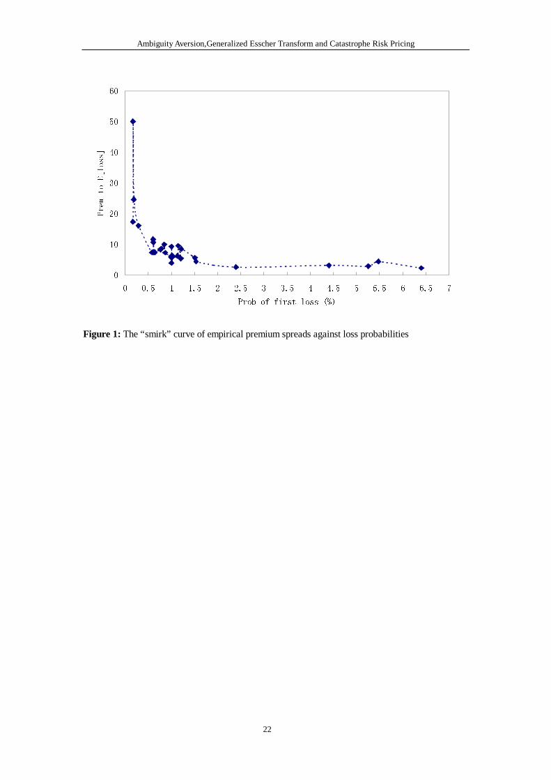
There is a second, more subtle point to be taken from Table 1. It appears that the premium spread
is much more pronounced for CAT bonds with low probability that a contingent loss payment to
the bond issuers will be triggered. This may generate a kind of “smirk” pattern in the
cross-sectional plot of the premium to E[loss] ratio against the probability of contingent loss (see
Figure 1). As a comparison, there is no apparent relation between the ratio and the expected loss
percentage conditional on a loss occurrence, which indicates that the premium implicit in CAT
bonds is mainly sensitive to the rareness of the catastrophe events.
With the above two empirical facts in mind, it is worth considerable interest to explore an
economic model explaining why spreads in the CAT bond market are so high and why, moving
from the CAT bonds with large probabilities of loss occurrence to lower ones, the premium
spreads become more pronounced. Based on the economic model, it will as well be interesting to
develop a methodology for pricing the CAT linked securities and reinsurance contracts.
Please insert Figure 1 about here
Previous literature on CAT bonds and other related catastrophe contracts could be roughly divided
into two major groups:
The first group of articles concentrated on the possible economic explanations for high spread
puzzle (See, e.g., Bantwal and Kunreuther (2000), Froot (1999)). For example, Bantwal and
Kunreuther suggested that myopic loss aversion and prospect theory, ambiguity aversion, selection
bias and threshold behavior, impact of worry and fixed cost of education may account for the
puzzle. The second group devotes to describe the pricing formula of CAT-linked contracts. See, for
example, Cummins and Geman (1995), Geman and Yor (1997), and Cummins, Lewis and Phillips
(1999).
One common problem with these researches is that they failed to explain the second empirical fact

Ambiguity Aversion,Generalized Esscher Transform and Catastrophe Risk Pricing
4
mentioned above, i.e., they did not try to explain why premium spreads become less pronounced
when we move from CAT bonds with low probabilities of loss occurrence to larger ones. Another
problem is that most CAT risk pricing formulas are still based on a rather perfect framework and
did not account for the imperfect properties of agent behavior as listed in Bantwal and Kunreuther
(2000) into their models.
In this paper, we will introduce a kind of generalized Esscher transform for the pricing of CAT risk.
The generalized transform will be supported by an economic model describing the agent behavior
of ambiguity aversion in the sense of Anderson, Hansen and Sargent (2000). To explain the second
empirical fact mentioned above, we examine the implications of varying ambiguity aversion
toward rareness of catastrophe events. Without considering ambiguity aversion, our generalized
transform will be reduced to the Esscher transform introduced in Gerber and Shiu (1994). From
this perspective, this paper can be viewed as an addition to the list of many actuarial and financial
researches contributing to the generalization of the original Gerber-Shiu framework.
The rest of the paper is organized as follows. Section 2 proposes a kind of generalized Esscher
transform for compound Poisson process risk pricing and sets up an economic equilibrium model
to examine the economic implication of the generalized transform. Section 3 demonstrates how to
use the transform to price the catastrophe-linked contracts. This section also presents an estimation
of the model using the 1997-2000 CAT bonds data and evaluates the model efficiency by
examining 2000-2003 CAT bonds data. Section 4 concludes. Technical details are collected in the
Appendix.
2. Generalized Esscher Transform and Economic Implications
2.1 Stochastic Discount Factor and Generalized Esscher Transform
Over the past several decades, there appears a tendency towards a unification of financial
economics and actuarial theories. Both insurance and finance are interested in the fair pricing of
financial products and the theoretical and empirical developments for asset pricing in both fields
currently become emphasizing the concept of “stochastic discount factor” that relates payoffs for

Ambiguity Aversion,Generalized Esscher Transform and Catastrophe Risk Pricing
5
contingent claims to market prices in an equilibrium market.
The basic equation for the stochastic discount factor can be written as follows:
]),([E Ttt ZTtC η= , (2.1)
whereCt is the time-t price of a contingent claim with random payoffZT at time T; Et is the
conditional expectation operator conditioning on the information available up to timet, and
),( Ttη is the so-called stochastic discount factor, or SDF.
If markets are complete, then the stochastic discount factor is unique. But complete case is rare in
insurance and as a consequence, there will be infinitely many such stochastic state prices so a
natural question to come in this case is which stochastic discount factor should be applied. A
particularly tractable specification for the stochastic discount factor is
)(/)())(exp(),( tTtTTt ζζδη −−= ,
and )(tζ has the form
/)exp();()( tXtt ααζζ == )][exp(E tXα ,
whereXt is a specified risk process;δ is the risk-free continuously compounded interest rate.
α is a real number parameter andE is the expectation operator. This form of SDF is called
Esscher transform, which can be dated back to the Swedish actuary F. Esscher. Gerber and Shiu
(1994) pioneered the use of Esscher transform as a kind of SDF and applied it in pricing stock
options.
Esscher transform specified in Gerber and Shiu (1994) involves only one free parameter, which is
related with the risk aversion coefficient, and is thus still within the subjective expected utility
framework. As explained in the introduction, the traditional economic theory based on subjective
expected utility function has difficulty explaining the high premium spread of CAT bonds and
spread discrepancy of bonds with different loss probabilities. As a consequence, the traditional
Esscher transform seems not proper as a pricing principle assigning premium to catastrophe risk.
Thus in this paper we develop a generalized Esscher transform to price CAT risk.

Ambiguity Aversion,Generalized Esscher Transform and Catastrophe Risk Pricing
6
Since CAT losses is usually described as a compound Poisson process, the following argument
will be applied to a general riskYt which follows a compound Poisson process; that is,
Yt=∑=
tN
jjL
1
, (2.2)
whereNt is a Poisson process with intensityλ>0 andLj (j=1,2,�), independent of each other and
Nt, denotes the random loss amount. For convenience, we will assume the random loss variableLj
can be described by identical distribution function, )()Pr( xFxL Lj =≤ , whereFL(x) denotes the
distribution function of a random variableL.
For the risk process {Yt} specified above, we define )(tζ to have the following generalized
form:
)][exp(E/)exp(),;()( tttt NYNYtt βαβαβαζζ ++== . (2.3)
Let F(x;t) be the distribution function ofYt, i.e., )Pr();( xYtxF t ≤= , the generalized Esscher
transform ofYt is thus defined as a random variable having the cumulative distribution function
)],;()([E),;,( βαζβα txYItxF t ≤= , where )(⋅I denotes an event indicator function.
In other words, for generalized Esscher tansform besides applying Esscher transform to the
original CAT loss process to represent risk aversion, we augment an Esscher transform applying
only to Poisson processNt to represent ambiguity aversion of agents. In next section, it is shown
that this form of SDF is supported by an equilibrium economy with agents who are averse not only
to risk but also to uncertainty with respect to loss occurrence in a robust control framework.
Similar to the derivation in Gerber and Shiu (1994), the corresponding moment-generating
function of the random variableYt under the generalized Esscher transform can then be calculated
as
)]][exp(E/))[exp((E),;,( ttttY NYNYztzM βαβαβα +++=
Ambiguity Aversion,Generalized Esscher Transform and Catastrophe Risk Pricing
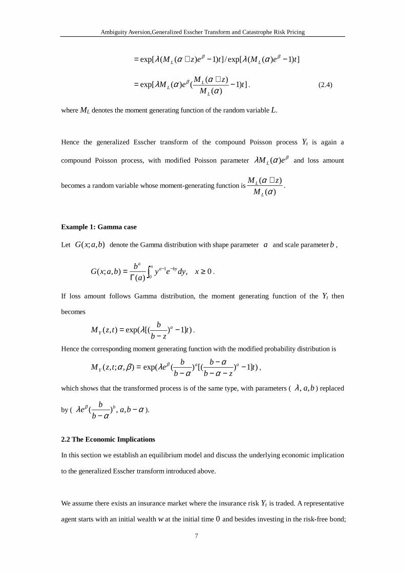
7
])1)((exp[/])1)((exp[ teMtezM LL −−+= ββ αλαλ
])1)(
)(()(exp[ t
M
zMeM
L
LL −+=
αααλ β . (2.4)
whereML denotes the moment generating function of the random variableL.
Hence the generalized Esscher transform of the compound Poisson processYt is again a
compound Poisson process, with modified Poisson parameter βαλ eM L )( and loss amount
becomes a random variable whose moment-generating function is)(
)(
ααL
L
M
zM +.
Example 1: Gamma case
Let ),;( baxG denote the Gamma distribution with shape parametera and scale parameterb ,
∫ ≥Γ
= −−x byaa
xdyeya
bbaxG
0
1 0,)(
),;( .
If loss amount follows Gamma distribution, the moment generating function of theYt then
becomes
)]1)[(exp(),( tzb
btzM a
Y −−
= λ .
Hence the corresponding moment generating function with the modified probability distribution is
=),;,( βαtzMY )]1)[()(exp( tzb
b
b
be aa −
−−−
− αα
αλ β ,
which shows that the transformed process is of the same type, with parameters (ba,,λ ) replaced
by ( αα
λ β −−
bab
be b ,,)( ).
2.2 The Economic Implications
In this section we establish an equilibrium model and discuss the underlying economic implication
to the generalized Esscher transform introduced above.
We assume there exists an insurance market where the insurance riskYt is traded. A representative
agent starts with an initial wealthw at the initial time0 and besides investing in the risk-free bond;
Ambiguity Aversion,Generalized Esscher Transform and Catastrophe Risk Pricing
8
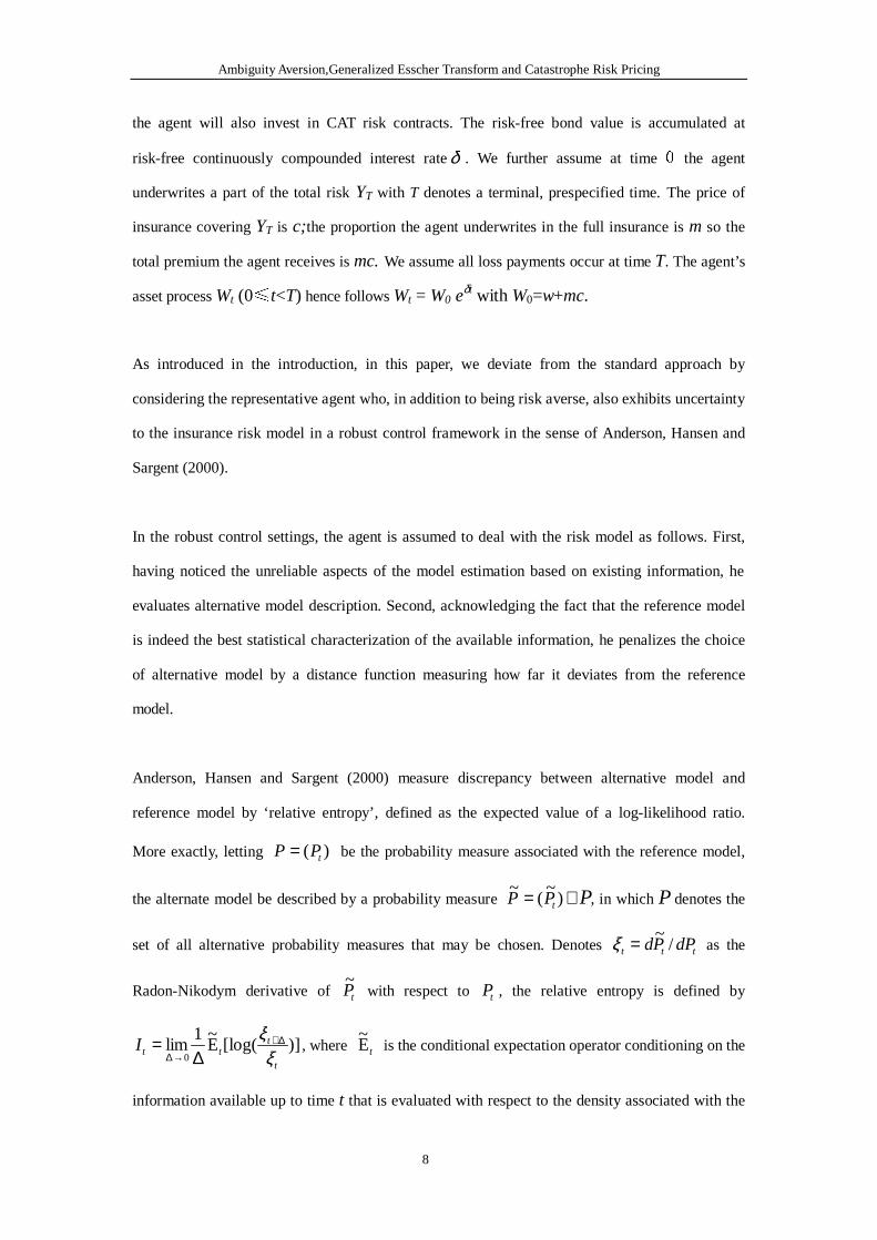
the agent will also invest in CAT risk contracts. The risk-free bond value is accumulated at
risk-free continuously compounded interest rateδ . We further assume at time��the agent
underwrites a part of the total riskYT with T denotes a terminal, prespecified time. The price of
insurance coveringYT is c;the proportion the agent underwrites in the full insurance ism so the
total premium the agent receives ismc.We assume all loss payments occur at timeT. The agent’s
asset processWt (0�t<T) hence followsWt = W0 eδt with W0=w+mc.
As introduced in the introduction, in this paper, we deviate from the standard approach by
considering the representative agent who, in addition to being risk averse, also exhibits uncertainty
to the insurance risk model in a robust control framework in the sense of Anderson, Hansen and
Sargent (2000).
In the robust control settings, the agent is assumed to deal with the risk model as follows. First,
having noticed the unreliable aspects of the model estimation based on existing information, he
evaluates alternative model description. Second, acknowledging the fact that the reference model
is indeed the best statistical characterization of the available information, he penalizes the choice
of alternative model by a distance function measuring how far it deviates from the reference
model.
Anderson, Hansen and Sargent (2000) measure discrepancy between alternative model and
reference model by ‘relative entropy’, defined as the expected value of a log-likelihood ratio.
More exactly, letting )( tPP = be the probability measure associated with the reference model,
the alternate model be described by a probability measure ∈= )~
(~
tPP P, in which P denotes the
set of all alternative probability measures that may be chosen. Denotes ttt dPPd /~=ξ as the
Radon-Nikodym derivative of tP~
with respect to tP , the relative entropy is defined by
)][log(E~1
lim0
t
tttI
ξξ ∆+
→∆ ∆= , where tE
~is the conditional expectation operator conditioning on the
information available up to timet that is evaluated with respect to the density associated with the

Ambiguity Aversion,Generalized Esscher Transform and Catastrophe Risk Pricing
9
alternative or twisted model (i.e., not the reference model).
We now turn to the optimization problem according to the spirit of robust control theory (See, e.g.,
Liu, Pan and Wang (2005)), we assume the agent seeks to maximize the robust-control utility
functionU, which is defined as the solution to the following stochastic integral equation:
),,,( mytWUU = )([E~
{inf~ TTtP
mYWu −=∈P
]},),,,(
yYWWdsmYsWUI
tt
T
t
sss ==− ∫ −
φγ
, (2.5)
with boundary condition )(),,,( myWumyTWU −= , where tE~
is the conditional
expectation operator with respect to an alternative probability measure inP; u is the exponential
utility function expressed as xexu γγ −−= )/1()( , and γ >0 is the risk coefficient;
∫ −T
t
sss dsmYsWUI
φγ ),,,(
represents a penalty function controlling the deviation from the
reference model, in whichφ is a parameter measuring the relative importance of the reference
and alternative models (In other words, an agent with higherφ exhibits higher aversion to model
uncertainty).
Since there seems no apparent relation between spread premium and loss severity for CAT
securities, we restrict here that the uncertainty aversion of the agent only applies to the likelihood
component of the loss arrival. That is, we effectively assume the agent only has doubt about the
occurrence probability of loss events, while is comfortable with the loss magnitude aspect of the
model. The Radon-Nikodym derivativetξ is thus defined by the following stochastic differential
equation.
dtedNed th
tth
ttt λξξξ )1()1( −−−= −
where ht is a time dependent function controlling the model distortion magnitude, and where
10 =ξ . By construction, the process }0,{ Ttt ≤≤ξ is a martingale of mean one. The
measure )~
(~
tPP = thus defined is indeed a probability measure, and letP be the entire

Ambiguity Aversion,Generalized Esscher Transform and Catastrophe Risk Pricing
10
collection of such probability measures.
Given the alternative model specification defined bytξ , the distance measureIt can be calculated
as:
It= )1( +− tt ht
h eheλ . (2.7)
See Appendix B in Liu, Pan and Wang (2005) for the proof of a more general formula than (2.7).
The equation (2.5) for utility functionU then becomes
),,,( mytWUU = )([E~
{inf}{ TTth
mYWus
−=
]},),,,(])1(1[ yYWWdsmYsWUeh tt
T
t ssh
ss ==−+− ∫ −φ
λγ
The corresponding HJB equation forU is then as follows:
Wt WUU δ+ ),,,(E[{inf mLytWUe t
t
h
h++ λ
}])1(1[)],,,( UehmytWU tht −+−−
φλγ
=0, (2.8)
whereUt is the derivative ofU with respect tot, UW, UWW are its first and second derivatives
with respect toW, and the terminal condition is )exp(1
),,,( WmyTWU γγ
−−= .
We conjecture that the indirect functionU is of the form
),(),(),,,( mtfetWVmytWU myγ= (2.9)
where V(W,t) is defined as )exp(1
),( )( tTWetWV −−−= δγγ
, and f(t,m) is a time-dependent
function.
Insert the form ofU in (2.9) into the above HJB equation and canceling the factor ofmyeγ , we can
then rewrite (2.8) as
Ambiguity Aversion,Generalized Esscher Transform and Catastrophe Risk Pricing
11
fWVVffV Wtt δ++
}])1(1[))][exp(E({inf VfehVfVfLme tt
t
ht
h
h−+−−+
φλγγλ =0. (2.10)
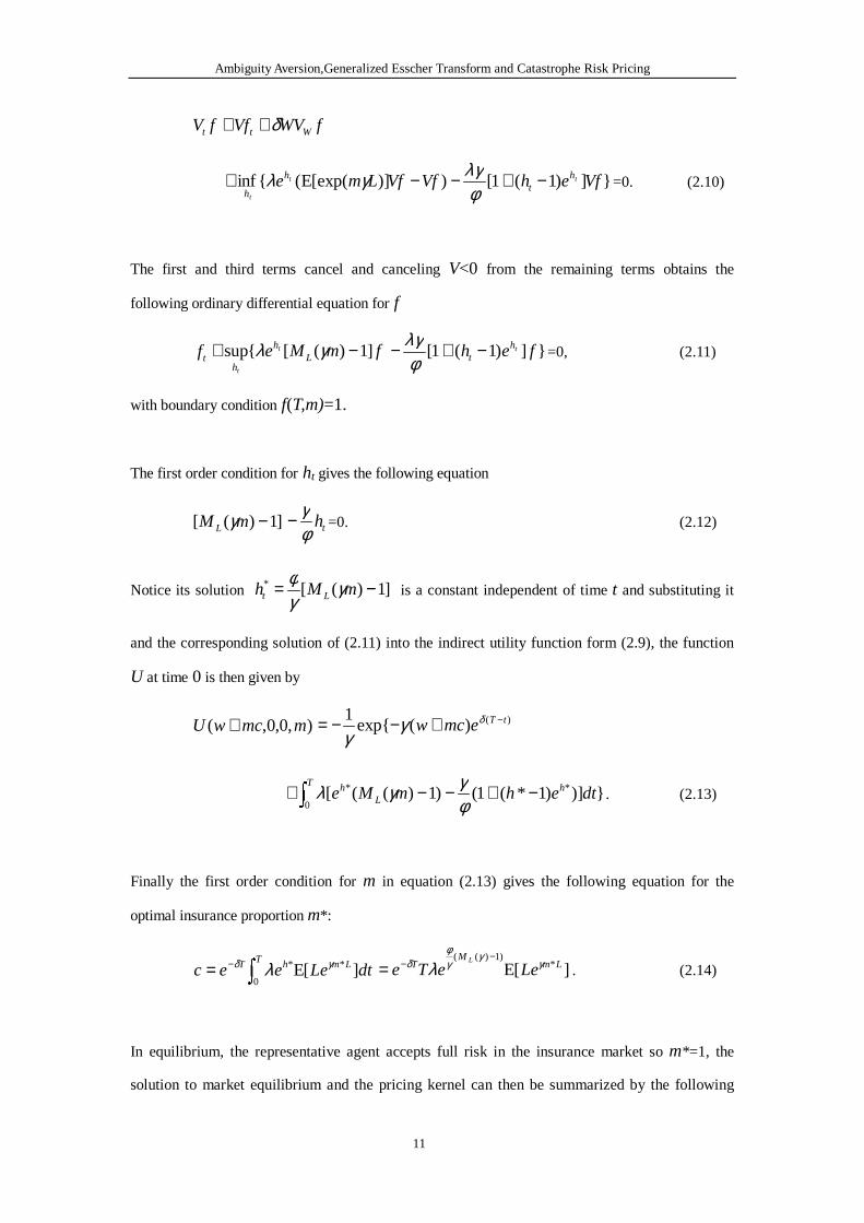
The first and third terms cancel and cancelingV<0 from the remaining terms obtains the
following ordinary differential equation forf
tf fmMe Lh
h
t
t
]1)([{sup −+ γλ }])1(1[ feh tht −+−
φλγ
=0, (2.11)
with boundary condition f(T,m)=1.
The first order condition forht gives the following equation
]1)([ −mM L γ thφγ− =0. (2.12)
Notice its solution ]1)([* −= mMh Lt γγφ
is a constant independent of timet and substituting it
and the corresponding solution of (2.11) into the indirect utility function form (2.9), the function
U at time0 is then given by
),0,0,( mmcwU + )()(exp{1 tTemcw −+−−= δγγ
∫ −+−−+T h
Lh dtehmMe
0
** })])1*(1()1)(([φγγλ . (2.13)
Finally the first order condition form in equation (2.13) gives the following equation for the
optimal insurance proportionm*:
∫−=
T LmhT dtLeeec0
** ][E γδ λ ][E *)1)((
LmM
T LeeTeL γ
γγφ
δ λ−
−= . (2.14)
In equilibrium, the representative agent accepts full risk in the insurance market som*=1, the
solution to market equilibrium and the pricing kernel can then be summarized by the following
Ambiguity Aversion,Generalized Esscher Transform and Catastrophe Risk Pricing
12
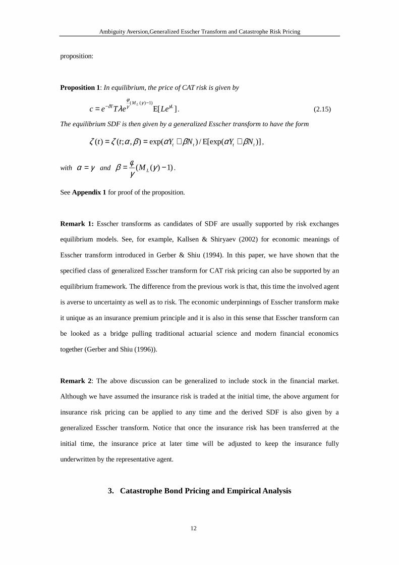
proposition:
Proposition 1: In equilibrium, the price of CAT risk is given by
][E)1)((
LM
T LeeTecL γ
γγφ
δ λ−
−= . (2.15)
The equilibrium SDF is then given by a generalized Esscher transform to have the form
)][exp(E/)exp(),;()( tttt NYNYtt βαβαβαζζ ++== ,
with γα = and )1)(( −= γγφβ LM .
SeeAppendix 1 for proof of the proposition.
Remark 1: Esscher transforms as candidates of SDF are usually supported by risk exchanges
equilibrium models. See, for example, Kallsen & Shiryaev (2002) for economic meanings of
Esscher transform introduced in Gerber & Shiu (1994). In this paper, we have shown that the
specified class of generalized Esscher transform for CAT risk pricing can also be supported by an
equilibrium framework. The difference from the previous work is that, this time the involved agent
is averse to uncertainty as well as to risk. The economic underpinnings of Esscher transform make
it unique as an insurance premium principle and it is also in this sense that Esscher transform can
be looked as a bridge pulling traditional actuarial science and modern financial economics
together (Gerber and Shiu (1996)).
Remark 2: The above discussion can be generalized to include stock in the financial market.
Although we have assumed the insurance risk is traded at the initial time, the above argument for
insurance risk pricing can be applied to any time and the derived SDF is also given by a
generalized Esscher transform. Notice that once the insurance risk has been transferred at the
initial time, the insurance price at later time will be adjusted to keep the insurance fully
underwritten by the representative agent.
3. Catastrophe Bond Pricing and Empirical Analysis

Ambiguity Aversion,Generalized Esscher Transform and Catastrophe Risk Pricing
13
3.1. Catastrophe Bond Pricing
In this section, we apply the SDF corresponding to the generalized Esscher transform to price CAT
bond. We assume for convenience of discussion that the form of CAT bond is described as
follows:
The CAT bond is priced atK, which denotes the bond principal. If the loss for any single CAT
event in the period(0, T) is less than a loss triggerA, the agent will get back his principalK, plus
risk-free interest )1( −TeK δ , plus spread premium lK~
at the maturity timeT, in which l~
denotes the spread premium rate. Once a CAT loss exceeds the trigger, the agent will forfeit some
or all the principal at timeT. We assume the spread premium plus the risk-free interest is
guaranteed no matter whether any principal loss occurs.
The aggregate CAT losses exceedingA in the time period(0, T) is assumed to follow a compound
Poisson distribution described as follows,
YT=∑=
TN
jjL
1
, (2.2)
where CAT (larger thanA) occurrences numberNT is Poisson with intensityλT>0 and Lj
(j=1,2,�), independent of each other andNT, denotes the random loss amount and can be
described by identical distribution function, )()Pr( xFxL Lj =≤ , where FL(x) denotes the
distribution function of a random variableL which is larger thanA.
The loss fractionfABof the principal is in proportion to the first CAT lossL1 in the range between
the trigger (A) and a cap (B), and is given by
)/()],(,0[ 1 ABABALMinMaxf AB −−−=
)/(]),0[],0[( 11 ABBLMaxALMax −−−−=
)/())(( 11 ABBLAL −−−−= + (3.1)
In other words, the cash flow the agent get back at timeT can be described as a random variable
Ambiguity Aversion,Generalized Esscher Transform and Catastrophe Risk Pricing
14
))0(~
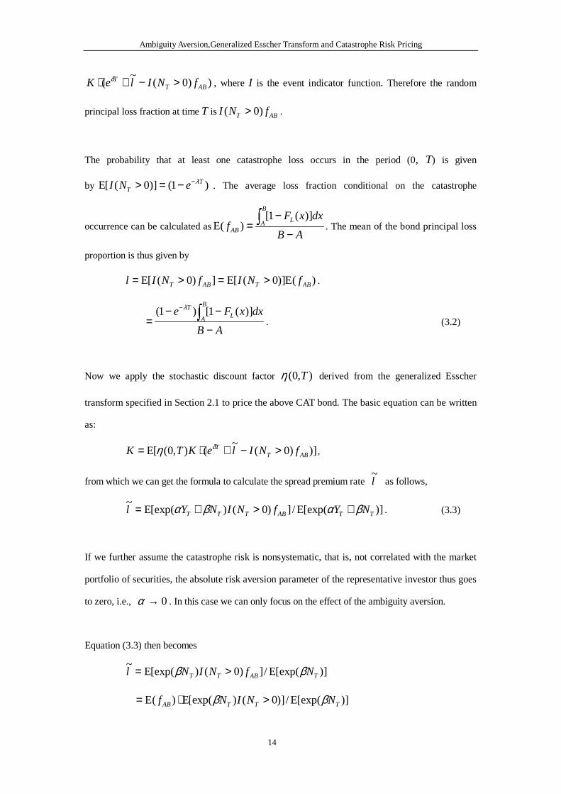
( ABTT fNIleK >−+⋅ δ , whereI is the event indicator function. Therefore the random
principal loss fraction at timeT is ABT fNI )0( > .
The probability that at least one catastrophe loss occurs in the period (0, T) is given
by )1()]0([E TT eNI λ−−=> . The average loss fraction conditional on the catastrophe
occurrence can be calculated asAB
dxxFf
B
A L
AB −
−= ∫ )](1[
)(E . The mean of the bond principal loss
proportion is thus given by
)(E)]0([E])0([E ABTABT fNIfNIl >=>= .
AB
dxxFeB
A LT
−
−−= ∫
− )](1[)1( λ
. (3.2)
Now we apply the stochastic discount factor ),0( Tη derived from the generalized Esscher
transform specified in Section 2.1 to price the above CAT bond. The basic equation can be written
as:
)])0(~
(),0([E ABTT fNIleKTK >−+⋅= δη ,
from which we can get the formula to calculate the spread premium ratel~
as follows,
)][exp(E/])0()[exp(E~
TTABTTT NYfNINYl βαβα +>+= . (3.3)
If we further assume the catastrophe risk is nonsystematic, that is, not correlated with the market
portfolio of securities, the absolute risk aversion parameter of the representative investor thus goes
to zero, i.e., 0→α . In this case we can only focus on the effect of the ambiguity aversion.
Equation (3.3) then becomes
)][exp(E/])0()[exp(E~
TABTT NfNINl ββ >=
)][exp(E/)]0()[exp(E)(E TTTAB NNINf ββ >⋅=
Ambiguity Aversion,Generalized Esscher Transform and Catastrophe Risk Pricing
15
in which )][exp(E/)]0()[exp(E TTT NNIN ββ > is the modified probability that at least one
catastrophe loss occurs and can be calculated to beβλTee−−1 . Therefore we
haveAB
dxxFel
B
A LTe
−
−−= ∫
− )](1[)1(~βλ
, and the ratio of the spread premium to the mean principal
loss can be given by the following proposition:
Proposition 2: Assuming the representative agent is risk neutral to the catastrophe riskYT, the
ratio of spread premium rate to the expected principle loss proportion (i.e., the ratio of the
modified mean principal loss to the expected loss) of the related CAT bonds is given by
ββ
λ
λ
λλ
β
eT
Te
e
e
l
lT
Te
=≈−
−= −
−
11
~, (3.4)
in which the second approximation equation holds whenλ is very small.
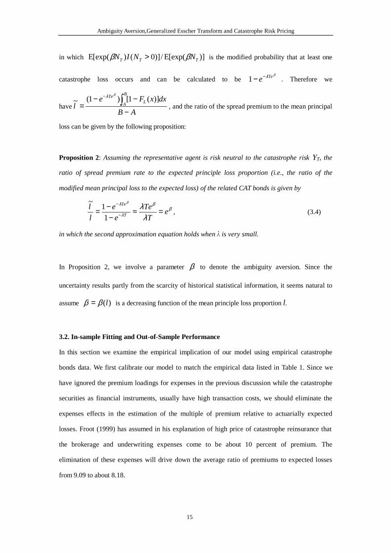
In Proposition 2, we involve a parameterβ to denote the ambiguity aversion. Since the
uncertainty results partly from the scarcity of historical statistical information, it seems natural to
assume )(lββ = is a decreasing function of the mean principle loss proportionl.
3.2. In-sample Fitting and Out-of-Sample Performance
In this section we examine the empirical implication of our model using empirical catastrophe
bonds data. We first calibrate our model to match the empirical data listed in Table 1. Since we
have ignored the premium loadings for expenses in the previous discussion while the catastrophe
securities as financial instruments, usually have high transaction costs, we should eliminate the
expenses effects in the estimation of the multiple of premium relative to actuarially expected
losses. Froot (1999) has assumed in his explanation of high price of catastrophe reinsurance that
the brokerage and underwriting expenses come to be about 10 percent of premium. The
elimination of these expenses will drive down the average ratio of premiums to expected losses
from 9.09 to about 8.18.
Ambiguity Aversion,Generalized Esscher Transform and Catastrophe Risk Pricing
16
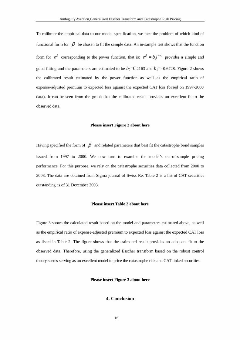
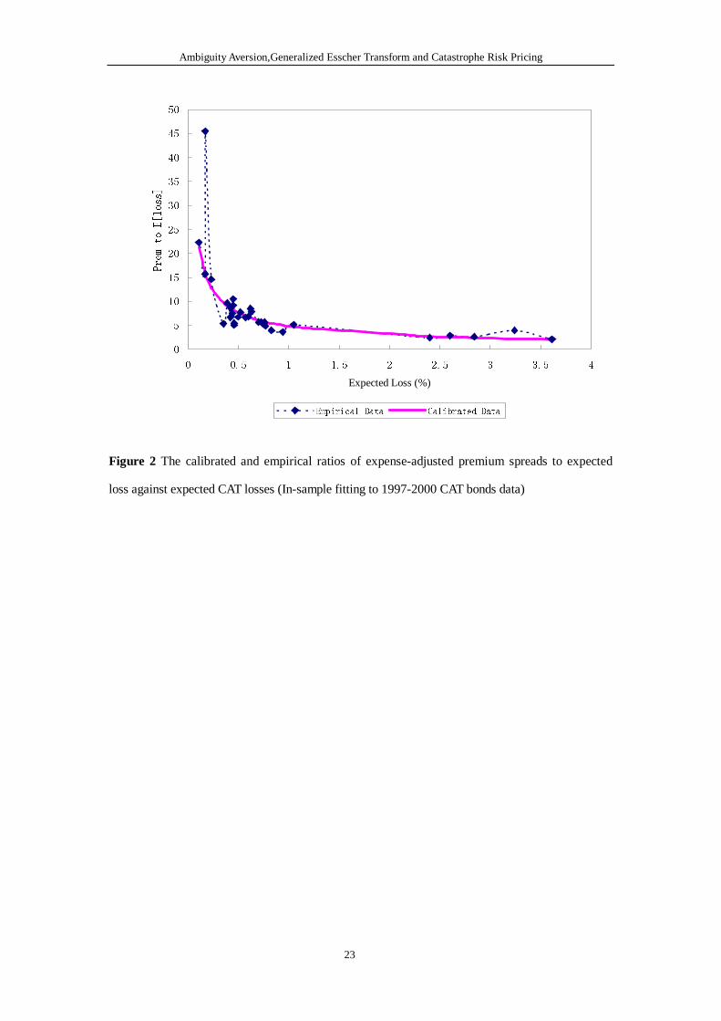
To calibrate the empirical data to our model specification, we face the problem of which kind of
functional form for β be chosen to fit the sample data. An in-sample test shows that the function
form for βe corresponding to the power function, that is: 1
0blbe −=β provides a simple and
good fitting and the parameters are estimated to beb0=0.2163 andb1=�0.6728. Figure 2 shows
the calibrated result estimated by the power function as well as the empirical ratio of
expense-adjusted premium to expected loss against the expected CAT loss (based on 1997-2000
data). It can be seen from the graph that the calibrated result provides an excellent fit to the
observed data.
Please insert Figure 2 about here
Having specified the form ofβ and related parameters that best fit the catastrophe bond samples
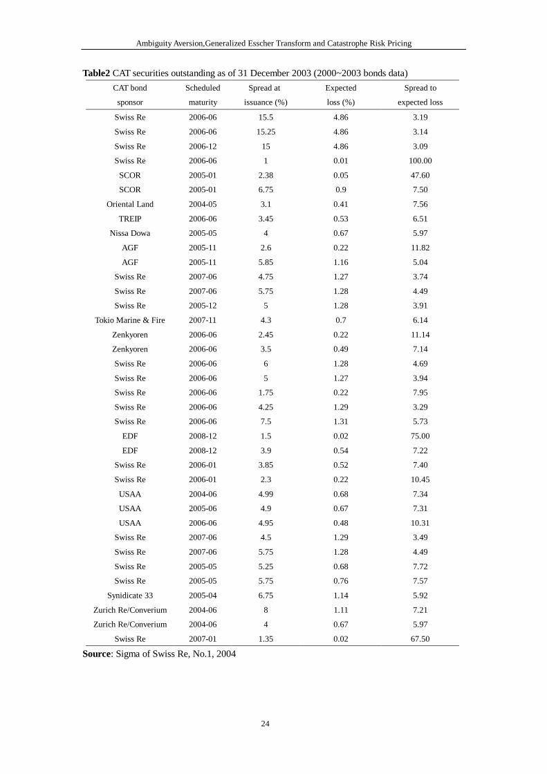
issued from 1997 to 2000. We now turn to examine the model’s out-of-sample pricing
performance. For this purpose, we rely on the catastrophe securities data collected from 2000 to
2003. The data are obtained from Sigma journal of Swiss Re. Table 2 is a list of CAT securities
outstanding as of 31 December2003.
Please insert Table 2 about here
Figure 3 shows the calculated result based on the model and parameters estimated above, as well
as the empirical ratio of expense-adjusted premium to expected loss against the expected CAT loss
as listed in Table 2. The figure shows that the estimated result provides an adequate fit to the
observed data. Therefore, using the generalized Esscher transform based on the robust control
theory seems serving as an excellent model to price the catastrophe risk and CAT linked securities.
Please insert Figure 3 about here
4. Conclusion
Ambiguity Aversion,Generalized Esscher Transform and Catastrophe Risk Pricing
17
Motivated by the observation that the spread premium of CAT loss securities is very high relative
to the expected loss of principal of bonds, and the premium spread is much more pronounced for
CAT bonds with low probability that a contingent loss payment to the bond issuers will be
triggered, we have extended the traditional Esscher Transform to a generalized framework and
treated it as a stochastic discount pricing factor to price the CAT risk. The generalized Esscher
transform is derived from a modified equilibrium model by allowing the representative agent to
act in a robust control framework against model misspecification with respect to rare events in the
sense of Anderson, Hansen and Sargent (2000). The model is explicitly solved and the derived
pricing kernel is shown to be exactly the generalized Esscher Transform. Using catastrophe bonds
data, we examine the empirical implication of our model.
There are several extensions we may do to our current investigation. First, we have considered the
issue of uncertainty aversion in a robust control framework and thus envision the model
misspecification as a permanent psychological characteristic of a decision maker. On the other
hand, an agent may learn the model through successive approximations. It would be an important
extension to incorporate forms of learning, i.e., the credibility theory, into our framework. Second,
we restrict the CAT loss process here to be a compound Poisson process. Since there is usually
seasonality in catastrophe occurrence, it will be interesting to describe the CAT loss by a
time-changed Levy process and in the most general setting, the process written as a
semimartingale. Discussion for the corresponding change of measure in these cases can be found
in Carr & Wu (2004), and B��lmann et al (1998). Finally, just as Froot pointed out (1999), there is
typically a shift of coverage window in reinsurance market after a large CAT event occurs. To
explain this time series empirical fact, it might be helpful to model how the prior performance of
CAT events might affect the magnitude of uncertainty aversion of decision makers in an insurance
market. For this purpose, we may simulate the approach on similar topic in the framework of
wealth-based prospect theory (see, e.g., the seminal contribution of Barberis, Huang and Santos
(2001)). For all these issues we leave for future research.
Ambiguity Aversion,Generalized Esscher Transform and Catastrophe Risk Pricing
18
Appendix 1
Proof of Proposition 1: According to equation (2.4), the moment generating function under the
generalized Esscher transform specified in Proposition 1 can be calculated as
])1)(
)(()(exp[),;,( t
M
zMeMtzM
L
LLY −+=
αααλβα β ,
with γα = and )1)(( −= γγφβ LM .
Hence the generalized Esscher transform ofYt is again a compound Poisson transform, with
modified Poisson parameter)1)((
)(−γ
γφ
γλLM
L eM and loss amount becomes a random variable
whose moment-generating function is)(
)(
γγL
L
M
zM +. The modified mean of loss amount can then
be calculated as
])(
[])(
[))(
)((
11γγγ
γ γγ
L
L
zL
zL
zL
L
M
eL
zM
eL
M
zM
dz
dEE ==+
==
.
Therefore the price of CAT riskYt in period (t, T) is given by
dtM
eLMeec
T
L
L
L
MT L
∫−
−=0
)1)((
])(
[E)(γ
γλγγ
γφ
δ
][E)1)((
LM
T LeeTeL γ
γγφ
δ λ−
−= .

Ambiguity Aversion,Generalized Esscher Transform and Catastrophe Risk Pricing
19
REFERENCES
1. Anderson, E, L.P. Hansen and T.J.Sargent, “Risk and Robustness in General Equilibrium,”
Working Paper, University of Chicago, 2000.
2. Bantwal, V.J. and H.C. Kunreuther, “A Cat Bond Premium Puzzle,”The Journal of
Psychology and Financial Market, 1(1): 76-91, 2000.
3. Barberis, N.C., M. Huang and T. Santos, “Prospect Theory and Asset Prices,”The Quarterly
Journal of Economics, 116: 1-53, 2001.
4. B�hlmann, H., F. Delbaen, P. Embrechts, and A. Shiryaev, “No-arbitrage, change of measure
and conditional Esscher transforms,”CWI Quartly,9: 291-317, 1996.
5. Carr, P. and L. Wu, “Time-Changed Levy Processes and Option Pricing,”Journal of
Financial Economics71: 113-141, 2004.
6. Cummins, J.D. and H. Geman, “Pricing Catastrophe Insurance Futures and Call Spreads: An
Arbitrage Approach,”Journal of Fixed Income4: 46-57, 1995.
7. Cummins, J.D., C.M. Lewis and R.D. Phillips, “Pricing Excess-of-Loss Reinsurance
Contracts against Catastrophic Loss,” in K. Froot, ed.,The Financing of Catastrophe Risk,
University of Chicago Press: 93-147, 1999.
8. Cummins, J.D., D.Lalonde and R.D.Phillips, “The Basis Risk of Catastrophic-loss Index
Securities,”Journal of Financial Economics71: 77-111, 2004.
9. Froot, Kenneth, “Introduction” to K. Froot, ed.,The Financing of Catastrophe Risk,
University of Chicago Press: 1-22, 1999.
10. Geman, H. and M. Yor, “Stochastic Time Changes in Catastrophe Option Pricing,”Insurance:
Mathematics and Economics,21(3): 567-590, 1997.
11. Gerber, H.U. and Shiu, E.S.W., “Option pricing by Esscher transforms,”Transactions of the
Society of Actuaries, XLVI, 99-191, 1994.
12. Gerber, H.U. and Shiu, E.S.W., “Actuarial bridges to Dynamic Hedging and Option Pricing,”
Insurance: Mathematics and Economics,18: 183-218, 1996.
13. Kallsen, J. and A.N. Shiryaev, “The Cumulant Process and Esscher’s Change of Measure, ”
Finance and Stochastics, 6: 397-428, 2002.
14. Liu J., J. Pan and T. Wang, “An Equilibrium Model of Rare-Event Premia,”Review of

Ambiguity Aversion,Generalized Esscher Transform and Catastrophe Risk Pricing
20
Financial Studies18(1): 131-164, 2005.
15. SwissRe, “Natural Catastrophes and Man-made Disasters in 2003: Many Fatalities,
Comparatively Moderate Insured Losses,”Sigma1:1-44, 2005.

Ambiguity Aversion,Generalized Esscher Transform and Catastrophe Risk Pricing
21
Table 1: Catastrophe bond issues (1997~2000 bonds data)
The Spread Premium is the annual coupon rate above one-year LIBOR. The Prob of First Loss is
the probability that a contingent payment will be trigged under the bond. The E[L�L>0] is the
expected principal payment to the issuing insurer, conditional on the occurrence of a loss that
triggers payment under the bond, expressed as a percentage of the principle of the bond. The
Expected Loss is the product of the probability of first loss and E[L�L>0]. Prem to E[loss] is the
ratio of the spread premium to the expected loss of principle of the bond.
Date TransactionSponsor
SpreadPremium (%)
Prob of FirstLoss (%)
E[L�L>0](%)
ExpectedLoss (%)
Prem toE[Loss]
March-00 SCOR 2.70 0.19 57.89 0.11 24.55March-00 SCOR 3.70 0.29 79.31 0.23 16.09March-00 SCOR 14.00 5.47 59.23 3.24 4.32March-00 Lehman Re 4.50 1.13 64.60 0.73 6.16November-99 American Re 2.95 0.17 100.00 0.17 17.35November-99 American Re 5.40 0.78 80.77 0.63 8.57November-99 American Re 8.50 0.17 100.00 0.17 50.00November-99 Gerling 4.50 1.00 75.00 0.75 6.00June-99 Gerling 5.20 0.60 75.00 0.45 11.56June-99 USAA 3.66 0.76 57.89 0.44 8.32July-99 Sorema 4.50 0.84 53.57 0.45 10.00July-98 Yasuda 3.70 1.00 94.00 0.94 3.94March-99 Kemper 3.69 0.58 86.21 0.50 7.38March-99 Kemper 4.50 0.62 96.77 0.60 7.50May-99 Oriental Land 3.10 0.64 66.04 0.42 7.35February-99 St. Paul/F&G Re 4.00 1.15 36.52 0.42 9.52February-99 St. Paul/F&G Re 8.25 5.25 54.10 2.84 2.90December-98 Center Solutions 4.17 1.20 64.17 0.77 5.42December-98 Allianz 8.22 6.40 56.41 3.61 2.28August-98 XL/MidOcean Re 4.12 0.61 63.93 0.39 10.56August-98 XL/MidOcean Re 5.90 1.50 70.00 1.05 5.62July-98 St. Paul/F&G Re 4.44 1.21 42.98 0.52 8.54July-98 St. Paul/F&G Re 8.27 4.40 59.09 2.60 3.18June-98 USAA 4.16 0.87 65.52 0.57 7.30March-98 Center Solutions 3.67 1.53 54.25 0.83 4.42December-97 Tokio Marine &
Fire2.09 1.02 34.71 0.35 5.90
December-97 Tokio Marine &Fire
4.36 1.02 68.63 0.70 6.23
July-97 USAA 5.76 1.00 62.00 0.62 9.29August-97 Swiss Re 2.55 1.00 45.60 0.46 5.59August-97 Swiss Re 2.80 1.00 46.00 0.46 6.09August-97 Swiss Re 4.75 1.00 76.00 0.76 6.25August-97 Swiss Re 6.25 2.40 100.00 2.40 2.60
AverageMedian
9.096.77
Source: Cummins, Lalonde and Phillips (2004)
Ambiguity Aversion,Generalized Esscher Transform and Catastrophe Risk Pricing
22
�
��
��
��
��
��
��
� ��� � ��� � ��� � ��� � ��� � ��� � ���
�� ������������������
�������������
Figure 1: The “smirk” curve of empirical premium spreads against loss probabilities
Ambiguity Aversion,Generalized Esscher Transform and Catastrophe Risk Pricing
23
�
�
��
��
��
��
��
��
��
��
��
� ��� � ��� � ��� � ��� �
Expected Loss (%)
�������������
������������ ���� ��������
Figure 2 The calibrated and empirical ratios of expense-adjusted premium spreads to expected
loss against expected CAT losses (In-sample fitting to 1997-2000 CAT bonds data)
Ambiguity Aversion,Generalized Esscher Transform and Catastrophe Risk Pricing
24
Table2 CAT securities outstanding as of 31 December2003 (2000~2003 bonds data)
Source: Sigma of Swiss Re, No.1, 2004
CAT bond
sponsor
Scheduled
maturity
Spread at
issuance (%)
Expected
loss (%)
Spread to
expected loss
Swiss Re 2006-06� 15.5� 4.86� 3.19�
Swiss Re 2006-06� 15.25� 4.86� 3.14�
Swiss Re 2006-12� 15� 4.86� 3.09�
Swiss Re 2006-06� 1� 0.01� 100.00�
SCOR 2005-01� 2.38� 0.05� 47.60�
SCOR 2005-01� 6.75� 0.9� 7.50�
Oriental Land 2004-05� 3.1� 0.41� 7.56�
TREIP 2006-06� 3.45� 0.53� 6.51�
Nissa Dowa 2005-05� 4� 0.67� 5.97�
AGF 2005-11� 2.6� 0.22� 11.82�
AGF 2005-11� 5.85� 1.16� 5.04�
Swiss Re 2007-06� 4.75� 1.27� 3.74�
Swiss Re 2007-06� 5.75� 1.28� 4.49�
Swiss Re 2005-12� 5� 1.28� 3.91�
Tokio Marine & Fire 2007-11� 4.3� 0.7� 6.14�
Zenkyoren 2006-06� 2.45� 0.22� 11.14�
Zenkyoren 2006-06� 3.5� 0.49� 7.14�
Swiss Re 2006-06� 6� 1.28� 4.69�
Swiss Re 2006-06� 5� 1.27� 3.94�
Swiss Re 2006-06� 1.75� 0.22� 7.95�
Swiss Re 2006-06� 4.25� 1.29� 3.29�
Swiss Re 2006-06� 7.5� 1.31� 5.73�
EDF 2008-12� 1.5� 0.02� 75.00�
EDF 2008-12� 3.9� 0.54� 7.22�
Swiss Re 2006-01� 3.85� 0.52� 7.40�
Swiss Re 2006-01� 2.3� 0.22� 10.45�
USAA 2004-06� 4.99� 0.68� 7.34�
USAA 2005-06� 4.9� 0.67� 7.31�
USAA 2006-06� 4.95� 0.48� 10.31�
Swiss Re 2007-06� 4.5� 1.29� 3.49�
Swiss Re 2007-06� 5.75� 1.28� 4.49�
Swiss Re 2005-05� 5.25� 0.68� 7.72�
Swiss Re 2005-05� 5.75� 0.76� 7.57�
Synidicate 33 2005-04� 6.75� 1.14� 5.92�
Zurich Re/Converium 2004-06� 8� 1.11� 7.21�
Zurich Re/Converium 2004-06� 4� 0.67� 5.97�
Swiss Re 2007-01� 1.35� 0.02� 67.50�

Ambiguity Aversion,Generalized Esscher Transform and Catastrophe Risk Pricing
25
�
��
��
��
��
���
���
� ��� � ��� � ��� �� � ��� � ���
Expected Loss��
�������������
������������ ���� ��������
Figure 3 The calibrated and empirical ratios of expense-adjusted premium spreads to expected
loss against expected CAT losses (Out of sample fitting to 2000~2003 CAT bonds data using
1997-2000 bonds data based estimation)