Embed Size (px)
Citation preview

Amberg TSP PlusSee ahead - build safer
Evaluation ManualVersion 1.2.1.0, 05/2015© Amberg Technologies AG, 2012-2015Art. No. 20847
Amberg Technologies AGTrockenloostrasse 218105 RegensdorfSwitzerland
Phone: +41 44 870 92 22Mail: [email protected]://www.amberg.ch/at


Evaluation Manual
© Amberg Technologies AG, 2012-2015 Page 3 of 106
Table of ContentsWelcome to Amberg TSP Plus . . . . . . . . . . . . . . . . . . . . . . . . . . . . . . . . . . . . . . . . . . . . . . . . . . . . . . . . . . . . . . . . . . . . . . . . . . . . . . . . . . . . . . . . . . . . . . . . . 7
1 Software licence agreement . . . . . . . . . . . . . . . . . . . . . . . . . . . . . . . . . . . . . . . . . . . . . . . . . . . . . . . . . . . . . . . . . . . . . . . . . . . . . . . . . . . . . . . . . . . 72 Software installation / licensing . . . . . . . . . . . . . . . . . . . . . . . . . . . . . . . . . . . . . . . . . . . . . . . . . . . . . . . . . . . . . . . . . . . . . . . . . . . . . . . . . . . . . . . 8
2.1 System requirements . . . . . . . . . . . . . . . . . . . . . . . . . . . . . . . . . . . . . . . . . . . . . . . . . . . . . . . . . . . . . . . . . . . . . . . . . . . . . . . . . . . . . . . . . . . 82.2 Software installation . . . . . . . . . . . . . . . . . . . . . . . . . . . . . . . . . . . . . . . . . . . . . . . . . . . . . . . . . . . . . . . . . . . . . . . . . . . . . . . . . . . . . . . . . . . . . 8
3 Use of manual . . . . . . . . . . . . . . . . . . . . . . . . . . . . . . . . . . . . . . . . . . . . . . . . . . . . . . . . . . . . . . . . . . . . . . . . . . . . . . . . . . . . . . . . . . . . . . . . . . . . . . . . . . . . . . . . . 93.1 Conventions used in this manual . . . . . . . . . . . . . . . . . . . . . . . . . . . . . . . . . . . . . . . . . . . . . . . . . . . . . . . . . . . . . . . . . . . . . . . . 9
4 Safety Directions . . . . . . . . . . . . . . . . . . . . . . . . . . . . . . . . . . . . . . . . . . . . . . . . . . . . . . . . . . . . . . . . . . . . . . . . . . . . . . . . . . . . . . . . . . . . . . . . . . . . . . . . . . . . . 94.1 Use of instrument . . . . . . . . . . . . . . . . . . . . . . . . . . . . . . . . . . . . . . . . . . . . . . . . . . . . . . . . . . . . . . . . . . . . . . . . . . . . . . . . . . . . . . . . . . . . . . . . . 104.2 Disclaimer of liability . . . . . . . . . . . . . . . . . . . . . . . . . . . . . . . . . . . . . . . . . . . . . . . . . . . . . . . . . . . . . . . . . . . . . . . . . . . . . . . . . . . . . . . . . . . . 11
1 General Introduction . . . . . . . . . . . . . . . . . . . . . . . . . . . . . . . . . . . . . . . . . . . . . . . . . . . . . . . . . . . . . . . . . . . . . . . . . . . . . . . . . . . . . . . . . . . . . . . . . . . . . . . . . . . . . . . . 131.1 General work flow . . . . . . . . . . . . . . . . . . . . . . . . . . . . . . . . . . . . . . . . . . . . . . . . . . . . . . . . . . . . . . . . . . . . . . . . . . . . . . . . . . . . . . . . . . . . . . . . . . . . . . . . 131.2 The TSP concept . . . . . . . . . . . . . . . . . . . . . . . . . . . . . . . . . . . . . . . . . . . . . . . . . . . . . . . . . . . . . . . . . . . . . . . . . . . . . . . . . . . . . . . . . . . . . . . . . . . . . . . . . 13
1.2.1 Project and Campaign . . . . . . . . . . . . . . . . . . . . . . . . . . . . . . . . . . . . . . . . . . . . . . . . . . . . . . . . . . . . . . . . . . . . . . . . . . . . . . . . . . . . . . 131.3 The TSP Coordinate system . . . . . . . . . . . . . . . . . . . . . . . . . . . . . . . . . . . . . . . . . . . . . . . . . . . . . . . . . . . . . . . . . . . . . . . . . . . . . . . . . . . . . . . 14
1.3.1 Bore hole properties . . . . . . . . . . . . . . . . . . . . . . . . . . . . . . . . . . . . . . . . . . . . . . . . . . . . . . . . . . . . . . . . . . . . . . . . . . . . . . . . . . . . . . . . . 161.4 Description of the work space . . . . . . . . . . . . . . . . . . . . . . . . . . . . . . . . . . . . . . . . . . . . . . . . . . . . . . . . . . . . . . . . . . . . . . . . . . . . . . . . . . . . . 20
1.4.1 Customizing workspace components . . . . . . . . . . . . . . . . . . . . . . . . . . . . . . . . . . . . . . . . . . . . . . . . . . . . . . . . . . . . . . . 211.5 General menu functions . . . . . . . . . . . . . . . . . . . . . . . . . . . . . . . . . . . . . . . . . . . . . . . . . . . . . . . . . . . . . . . . . . . . . . . . . . . . . . . . . . . . . . . . . . . . . . . 21
1.5.1 Menu File . . . . . . . . . . . . . . . . . . . . . . . . . . . . . . . . . . . . . . . . . . . . . . . . . . . . . . . . . . . . . . . . . . . . . . . . . . . . . . . . . . . . . . . . . . . . . . . . . . . . . . . . . . . 211.5.2 Menu View . . . . . . . . . . . . . . . . . . . . . . . . . . . . . . . . . . . . . . . . . . . . . . . . . . . . . . . . . . . . . . . . . . . . . . . . . . . . . . . . . . . . . . . . . . . . . . . . . . . . . . . . . 221.5.3 Menu Window . . . . . . . . . . . . . . . . . . . . . . . . . . . . . . . . . . . . . . . . . . . . . . . . . . . . . . . . . . . . . . . . . . . . . . . . . . . . . . . . . . . . . . . . . . . . . . . . . . . 221.5.4 Menu Help . . . . . . . . . . . . . . . . . . . . . . . . . . . . . . . . . . . . . . . . . . . . . . . . . . . . . . . . . . . . . . . . . . . . . . . . . . . . . . . . . . . . . . . . . . . . . . . . . . . . . . . . . 22
1.6 General toolbar . . . . . . . . . . . . . . . . . . . . . . . . . . . . . . . . . . . . . . . . . . . . . . . . . . . . . . . . . . . . . . . . . . . . . . . . . . . . . . . . . . . . . . . . . . . . . . . . . . . . . . . . . . . . 221.7 Program options . . . . . . . . . . . . . . . . . . . . . . . . . . . . . . . . . . . . . . . . . . . . . . . . . . . . . . . . . . . . . . . . . . . . . . . . . . . . . . . . . . . . . . . . . . . . . . . . . . . . . . . . . . . 23
1.7.1 General - Labels . . . . . . . . . . . . . . . . . . . . . . . . . . . . . . . . . . . . . . . . . . . . . . . . . . . . . . . . . . . . . . . . . . . . . . . . . . . . . . . . . . . . . . . . . . . . . . . 231.7.2 Graphics . . . . . . . . . . . . . . . . . . . . . . . . . . . . . . . . . . . . . . . . . . . . . . . . . . . . . . . . . . . . . . . . . . . . . . . . . . . . . . . . . . . . . . . . . . . . . . . . . . . . . . . . . . . . 241.7.3 Preferences - Language . . . . . . . . . . . . . . . . . . . . . . . . . . . . . . . . . . . . . . . . . . . . . . . . . . . . . . . . . . . . . . . . . . . . . . . . . . . . . . . . . . . 241.7.4 Preferences - Units . . . . . . . . . . . . . . . . . . . . . . . . . . . . . . . . . . . . . . . . . . . . . . . . . . . . . . . . . . . . . . . . . . . . . . . . . . . . . . . . . . . . . . . . . . . 25
1.8 Shortcuts . . . . . . . . . . . . . . . . . . . . . . . . . . . . . . . . . . . . . . . . . . . . . . . . . . . . . . . . . . . . . . . . . . . . . . . . . . . . . . . . . . . . . . . . . . . . . . . . . . . . . . . . . . . . . . . . . . . . . . . 262 Getting started . . . . . . . . . . . . . . . . . . . . . . . . . . . . . . . . . . . . . . . . . . . . . . . . . . . . . . . . . . . . . . . . . . . . . . . . . . . . . . . . . . . . . . . . . . . . . . . . . . . . . . . . . . . . . . . . . . . . . . . . . 27
2.1 Project . . . . . . . . . . . . . . . . . . . . . . . . . . . . . . . . . . . . . . . . . . . . . . . . . . . . . . . . . . . . . . . . . . . . . . . . . . . . . . . . . . . . . . . . . . . . . . . . . . . . . . . . . . . . . . . . . . . . . . . . . . . 272.1.1 New Project . . . . . . . . . . . . . . . . . . . . . . . . . . . . . . . . . . . . . . . . . . . . . . . . . . . . . . . . . . . . . . . . . . . . . . . . . . . . . . . . . . . . . . . . . . . . . . . . . . . . . . . 27
2.2 The TSP Project Tree . . . . . . . . . . . . . . . . . . . . . . . . . . . . . . . . . . . . . . . . . . . . . . . . . . . . . . . . . . . . . . . . . . . . . . . . . . . . . . . . . . . . . . . . . . . . . . . . . . 292.3 Rock Catalogue . . . . . . . . . . . . . . . . . . . . . . . . . . . . . . . . . . . . . . . . . . . . . . . . . . . . . . . . . . . . . . . . . . . . . . . . . . . . . . . . . . . . . . . . . . . . . . . . . . . . . . . . . . . . 302.4 Campaign . . . . . . . . . . . . . . . . . . . . . . . . . . . . . . . . . . . . . . . . . . . . . . . . . . . . . . . . . . . . . . . . . . . . . . . . . . . . . . . . . . . . . . . . . . . . . . . . . . . . . . . . . . . . . . . . . . . . . 32
2.4.1 Add Campaign... . . . . . . . . . . . . . . . . . . . . . . . . . . . . . . . . . . . . . . . . . . . . . . . . . . . . . . . . . . . . . . . . . . . . . . . . . . . . . . . . . . . . . . . . . . . . . . . 322.4.2 Import campaign... . . . . . . . . . . . . . . . . . . . . . . . . . . . . . . . . . . . . . . . . . . . . . . . . . . . . . . . . . . . . . . . . . . . . . . . . . . . . . . . . . . . . . . . . . . . . 342.4.3 Delete / Export . . . . . . . . . . . . . . . . . . . . . . . . . . . . . . . . . . . . . . . . . . . . . . . . . . . . . . . . . . . . . . . . . . . . . . . . . . . . . . . . . . . . . . . . . . . . . . . . . . 35
2.5 Acquisition . . . . . . . . . . . . . . . . . . . . . . . . . . . . . . . . . . . . . . . . . . . . . . . . . . . . . . . . . . . . . . . . . . . . . . . . . . . . . . . . . . . . . . . . . . . . . . . . . . . . . . . . . . . . . . . . . . . . 362.6 Shot data . . . . . . . . . . . . . . . . . . . . . . . . . . . . . . . . . . . . . . . . . . . . . . . . . . . . . . . . . . . . . . . . . . . . . . . . . . . . . . . . . . . . . . . . . . . . . . . . . . . . . . . . . . . . . . . . . . . . . . 36
2.6.1 Shot data toolbar . . . . . . . . . . . . . . . . . . . . . . . . . . . . . . . . . . . . . . . . . . . . . . . . . . . . . . . . . . . . . . . . . . . . . . . . . . . . . . . . . . . . . . . . . . . . . . 382.6.2 Shot data display options . . . . . . . . . . . . . . . . . . . . . . . . . . . . . . . . . . . . . . . . . . . . . . . . . . . . . . . . . . . . . . . . . . . . . . . . . . . . . . . . . 38
2.7 Geometry . . . . . . . . . . . . . . . . . . . . . . . . . . . . . . . . . . . . . . . . . . . . . . . . . . . . . . . . . . . . . . . . . . . . . . . . . . . . . . . . . . . . . . . . . . . . . . . . . . . . . . . . . . . . . . . . . . . . . . 392.7.1 Geometry toolbar . . . . . . . . . . . . . . . . . . . . . . . . . . . . . . . . . . . . . . . . . . . . . . . . . . . . . . . . . . . . . . . . . . . . . . . . . . . . . . . . . . . . . . . . . . . . . . 40
2.8 Profile . . . . . . . . . . . . . . . . . . . . . . . . . . . . . . . . . . . . . . . . . . . . . . . . . . . . . . . . . . . . . . . . . . . . . . . . . . . . . . . . . . . . . . . . . . . . . . . . . . . . . . . . . . . . . . . . . . . . . . . . . . . . 412.8.1 Add profile . . . . . . . . . . . . . . . . . . . . . . . . . . . . . . . . . . . . . . . . . . . . . . . . . . . . . . . . . . . . . . . . . . . . . . . . . . . . . . . . . . . . . . . . . . . . . . . . . . . . . . . . . 412.8.2 Edit profile . . . . . . . . . . . . . . . . . . . . . . . . . . . . . . . . . . . . . . . . . . . . . . . . . . . . . . . . . . . . . . . . . . . . . . . . . . . . . . . . . . . . . . . . . . . . . . . . . . . . . . . . . 422.8.3 Import/Export profile . . . . . . . . . . . . . . . . . . . . . . . . . . . . . . . . . . . . . . . . . . . . . . . . . . . . . . . . . . . . . . . . . . . . . . . . . . . . . . . . . . . . . . . . . . 42
2.9 Tunnel model . . . . . . . . . . . . . . . . . . . . . . . . . . . . . . . . . . . . . . . . . . . . . . . . . . . . . . . . . . . . . . . . . . . . . . . . . . . . . . . . . . . . . . . . . . . . . . . . . . . . . . . . . . . . . . . 43

Evaluation Manual Evaluation Manual
Page 4 of 106 © Amberg Technologies AG, 2012-2015
2.10 Receiver / Shot hole line . . . . . . . . . . . . . . . . . . . . . . . . . . . . . . . . . . . . . . . . . . . . . . . . . . . . . . . . . . . . . . . . . . . . . . . . . . . . . . . . . . . . . . . . . . . 432.10.1 Add/remove receiver . . . . . . . . . . . . . . . . . . . . . . . . . . . . . . . . . . . . . . . . . . . . . . . . . . . . . . . . . . . . . . . . . . . . . . . . . . . . . . . . . . . . . . . 442.10.2 Add/remove shot hole line . . . . . . . . . . . . . . . . . . . . . . . . . . . . . . . . . . . . . . . . . . . . . . . . . . . . . . . . . . . . . . . . . . . . . . . . . . . . . . 452.10.3 Add/remove shot hole . . . . . . . . . . . . . . . . . . . . . . . . . . . . . . . . . . . . . . . . . . . . . . . . . . . . . . . . . . . . . . . . . . . . . . . . . . . . . . . . . . . . . 462.10.4 Edit receiver and shot hole properties . . . . . . . . . . . . . . . . . . . . . . . . . . . . . . . . . . . . . . . . . . . . . . . . . . . . . . . . . . . 462.10.5 Copy/paste receiver and shot hole properties . . . . . . . . . . . . . . . . . . . . . . . . . . . . . . . . . . . . . . . . . . . . . . . 47
2.11 Data processing . . . . . . . . . . . . . . . . . . . . . . . . . . . . . . . . . . . . . . . . . . . . . . . . . . . . . . . . . . . . . . . . . . . . . . . . . . . . . . . . . . . . . . . . . . . . . . . . . . . . . . . . . 482.11.1 Add processing . . . . . . . . . . . . . . . . . . . . . . . . . . . . . . . . . . . . . . . . . . . . . . . . . . . . . . . . . . . . . . . . . . . . . . . . . . . . . . . . . . . . . . . . . . . . . . . 492.11.2 Survey setup . . . . . . . . . . . . . . . . . . . . . . . . . . . . . . . . . . . . . . . . . . . . . . . . . . . . . . . . . . . . . . . . . . . . . . . . . . . . . . . . . . . . . . . . . . . . . . . . . . . 502.11.3 Copy processing . . . . . . . . . . . . . . . . . . . . . . . . . . . . . . . . . . . . . . . . . . . . . . . . . . . . . . . . . . . . . . . . . . . . . . . . . . . . . . . . . . . . . . . . . . . . . 512.11.4 Delete processing . . . . . . . . . . . . . . . . . . . . . . . . . . . . . . . . . . . . . . . . . . . . . . . . . . . . . . . . . . . . . . . . . . . . . . . . . . . . . . . . . . . . . . . . . . . 52
3 Survey and 3D-Processing . . . . . . . . . . . . . . . . . . . . . . . . . . . . . . . . . . . . . . . . . . . . . . . . . . . . . . . . . . . . . . . . . . . . . . . . . . . . . . . . . . . . . . . . . . . . . . . . . . . . . 533.1 Processing setup . . . . . . . . . . . . . . . . . . . . . . . . . . . . . . . . . . . . . . . . . . . . . . . . . . . . . . . . . . . . . . . . . . . . . . . . . . . . . . . . . . . . . . . . . . . . . . . . . . . . . . . . . . 53
3.1.1 Processing monitor . . . . . . . . . . . . . . . . . . . . . . . . . . . . . . . . . . . . . . . . . . . . . . . . . . . . . . . . . . . . . . . . . . . . . . . . . . . . . . . . . . . . . . . . . . . 553.1.2 Trace view toolbar . . . . . . . . . . . . . . . . . . . . . . . . . . . . . . . . . . . . . . . . . . . . . . . . . . . . . . . . . . . . . . . . . . . . . . . . . . . . . . . . . . . . . . . . . . . . 573.1.3 Trace view options . . . . . . . . . . . . . . . . . . . . . . . . . . . . . . . . . . . . . . . . . . . . . . . . . . . . . . . . . . . . . . . . . . . . . . . . . . . . . . . . . . . . . . . . . . . . 573.1.4 Spectrum view . . . . . . . . . . . . . . . . . . . . . . . . . . . . . . . . . . . . . . . . . . . . . . . . . . . . . . . . . . . . . . . . . . . . . . . . . . . . . . . . . . . . . . . . . . . . . . . . . . . 593.1.5 Volume view toolbar . . . . . . . . . . . . . . . . . . . . . . . . . . . . . . . . . . . . . . . . . . . . . . . . . . . . . . . . . . . . . . . . . . . . . . . . . . . . . . . . . . . . . . . . . 603.1.6 Volume view options . . . . . . . . . . . . . . . . . . . . . . . . . . . . . . . . . . . . . . . . . . . . . . . . . . . . . . . . . . . . . . . . . . . . . . . . . . . . . . . . . . . . . . . . . 603.1.7 Histogram view . . . . . . . . . . . . . . . . . . . . . . . . . . . . . . . . . . . . . . . . . . . . . . . . . . . . . . . . . . . . . . . . . . . . . . . . . . . . . . . . . . . . . . . . . . . . . . . . . . 61
3.2 Step 1: Geometry Model . . . . . . . . . . . . . . . . . . . . . . . . . . . . . . . . . . . . . . . . . . . . . . . . . . . . . . . . . . . . . . . . . . . . . . . . . . . . . . . . . . . . . . . . . . . . . 633.3 Step 2: Offset Calculation . . . . . . . . . . . . . . . . . . . . . . . . . . . . . . . . . . . . . . . . . . . . . . . . . . . . . . . . . . . . . . . . . . . . . . . . . . . . . . . . . . . . . . . . . . . . 633.4 Step 3: Data Preparation . . . . . . . . . . . . . . . . . . . . . . . . . . . . . . . . . . . . . . . . . . . . . . . . . . . . . . . . . . . . . . . . . . . . . . . . . . . . . . . . . . . . . . . . . . . . . 633.5 Step 4: Data Rotation . . . . . . . . . . . . . . . . . . . . . . . . . . . . . . . . . . . . . . . . . . . . . . . . . . . . . . . . . . . . . . . . . . . . . . . . . . . . . . . . . . . . . . . . . . . . . . . . . . 643.6 Step 5: Data Setup . . . . . . . . . . . . . . . . . . . . . . . . . . . . . . . . . . . . . . . . . . . . . . . . . . . . . . . . . . . . . . . . . . . . . . . . . . . . . . . . . . . . . . . . . . . . . . . . . . . . . . 64
3.6.1 Data length . . . . . . . . . . . . . . . . . . . . . . . . . . . . . . . . . . . . . . . . . . . . . . . . . . . . . . . . . . . . . . . . . . . . . . . . . . . . . . . . . . . . . . . . . . . . . . . . . . . . . . . . 643.6.2 Zeroing . . . . . . . . . . . . . . . . . . . . . . . . . . . . . . . . . . . . . . . . . . . . . . . . . . . . . . . . . . . . . . . . . . . . . . . . . . . . . . . . . . . . . . . . . . . . . . . . . . . . . . . . . . . . . . . 653.6.3 Average Amplitude Spectrum . . . . . . . . . . . . . . . . . . . . . . . . . . . . . . . . . . . . . . . . . . . . . . . . . . . . . . . . . . . . . . . . . . . . . . . . . . . 653.6.4 Spectrogram . . . . . . . . . . . . . . . . . . . . . . . . . . . . . . . . . . . . . . . . . . . . . . . . . . . . . . . . . . . . . . . . . . . . . . . . . . . . . . . . . . . . . . . . . . . . . . . . . . . . . . 66
3.7 Step 6: Time Variant Highcut . . . . . . . . . . . . . . . . . . . . . . . . . . . . . . . . . . . . . . . . . . . . . . . . . . . . . . . . . . . . . . . . . . . . . . . . . . . . . . . . . . . . . . 673.7.1 Principle of time variant highcut filtering . . . . . . . . . . . . . . . . . . . . . . . . . . . . . . . . . . . . . . . . . . . . . . . . . . . . . . . . . . 67
3.8 Step 7: Band Pass Filter . . . . . . . . . . . . . . . . . . . . . . . . . . . . . . . . . . . . . . . . . . . . . . . . . . . . . . . . . . . . . . . . . . . . . . . . . . . . . . . . . . . . . . . . . . . . . 703.9 Step 8: First Arrival Picking . . . . . . . . . . . . . . . . . . . . . . . . . . . . . . . . . . . . . . . . . . . . . . . . . . . . . . . . . . . . . . . . . . . . . . . . . . . . . . . . . . . . . . . . . 713.10 Step 9: Pick Manager . . . . . . . . . . . . . . . . . . . . . . . . . . . . . . . . . . . . . . . . . . . . . . . . . . . . . . . . . . . . . . . . . . . . . . . . . . . . . . . . . . . . . . . . . . . . . . . . 723.11 Step 10: Pick Processing . . . . . . . . . . . . . . . . . . . . . . . . . . . . . . . . . . . . . . . . . . . . . . . . . . . . . . . . . . . . . . . . . . . . . . . . . . . . . . . . . . . . . . . . . . 74
3.11.1 Vp/Vs ratio & S-wave arrival . . . . . . . . . . . . . . . . . . . . . . . . . . . . . . . . . . . . . . . . . . . . . . . . . . . . . . . . . . . . . . . . . . . . . . . . . . 753.12 Step 11: Shot Energy Balance . . . . . . . . . . . . . . . . . . . . . . . . . . . . . . . . . . . . . . . . . . . . . . . . . . . . . . . . . . . . . . . . . . . . . . . . . . . . . . . . . . 763.13 Step 12: Q-estimation . . . . . . . . . . . . . . . . . . . . . . . . . . . . . . . . . . . . . . . . . . . . . . . . . . . . . . . . . . . . . . . . . . . . . . . . . . . . . . . . . . . . . . . . . . . . . . . . 763.14 Step 13: Reflected waves extraction . . . . . . . . . . . . . . . . . . . . . . . . . . . . . . . . . . . . . . . . . . . . . . . . . . . . . . . . . . . . . . . . . . . . . . . . . 773.15 Step 14: P.S. Separation . . . . . . . . . . . . . . . . . . . . . . . . . . . . . . . . . . . . . . . . . . . . . . . . . . . . . . . . . . . . . . . . . . . . . . . . . . . . . . . . . . . . . . . . . . . 793.16 Step 15: Preparation . . . . . . . . . . . . . . . . . . . . . . . . . . . . . . . . . . . . . . . . . . . . . . . . . . . . . . . . . . . . . . . . . . . . . . . . . . . . . . . . . . . . . . . . . . . . . . . . . . 793.17 Step 16: Velocity Analysis . . . . . . . . . . . . . . . . . . . . . . . . . . . . . . . . . . . . . . . . . . . . . . . . . . . . . . . . . . . . . . . . . . . . . . . . . . . . . . . . . . . . . . . . . 803.18 Step 17: Velocity Pick . . . . . . . . . . . . . . . . . . . . . . . . . . . . . . . . . . . . . . . . . . . . . . . . . . . . . . . . . . . . . . . . . . . . . . . . . . . . . . . . . . . . . . . . . . . . . . . . 813.19 Step 18: Depth Migration . . . . . . . . . . . . . . . . . . . . . . . . . . . . . . . . . . . . . . . . . . . . . . . . . . . . . . . . . . . . . . . . . . . . . . . . . . . . . . . . . . . . . . . . . . . 813.20 Step 19: Event extraction . . . . . . . . . . . . . . . . . . . . . . . . . . . . . . . . . . . . . . . . . . . . . . . . . . . . . . . . . . . . . . . . . . . . . . . . . . . . . . . . . . . . . . . . . . 823.21 Step 20: Reflector extraction . . . . . . . . . . . . . . . . . . . . . . . . . . . . . . . . . . . . . . . . . . . . . . . . . . . . . . . . . . . . . . . . . . . . . . . . . . . . . . . . . . . . . 82
4 Result Evaluation . . . . . . . . . . . . . . . . . . . . . . . . . . . . . . . . . . . . . . . . . . . . . . . . . . . . . . . . . . . . . . . . . . . . . . . . . . . . . . . . . . . . . . . . . . . . . . . . . . . . . . . . . . . . . . . . . . . . 854.1 Evaluation set . . . . . . . . . . . . . . . . . . . . . . . . . . . . . . . . . . . . . . . . . . . . . . . . . . . . . . . . . . . . . . . . . . . . . . . . . . . . . . . . . . . . . . . . . . . . . . . . . . . . . . . . . . . . . . . 85
4.1.1 Evaluation set toolbar . . . . . . . . . . . . . . . . . . . . . . . . . . . . . . . . . . . . . . . . . . . . . . . . . . . . . . . . . . . . . . . . . . . . . . . . . . . . . . . . . . . . . . . 864.1.2 Evaluation set view options . . . . . . . . . . . . . . . . . . . . . . . . . . . . . . . . . . . . . . . . . . . . . . . . . . . . . . . . . . . . . . . . . . . . . . . . . . . . . . 864.1.3 Charts view . . . . . . . . . . . . . . . . . . . . . . . . . . . . . . . . . . . . . . . . . . . . . . . . . . . . . . . . . . . . . . . . . . . . . . . . . . . . . . . . . . . . . . . . . . . . . . . . . . . . . . . . 894.1.4 2D/3D views . . . . . . . . . . . . . . . . . . . . . . . . . . . . . . . . . . . . . . . . . . . . . . . . . . . . . . . . . . . . . . . . . . . . . . . . . . . . . . . . . . . . . . . . . . . . . . . . . . . . . . 90

Evaluation Manual Evaluation Manual
© Amberg Technologies AG, 2012-2015 Page 5 of 106
4.1.5 Reflector table . . . . . . . . . . . . . . . . . . . . . . . . . . . . . . . . . . . . . . . . . . . . . . . . . . . . . . . . . . . . . . . . . . . . . . . . . . . . . . . . . . . . . . . . . . . . . . . . . . . 945 Result presentation and report . . . . . . . . . . . . . . . . . . . . . . . . . . . . . . . . . . . . . . . . . . . . . . . . . . . . . . . . . . . . . . . . . . . . . . . . . . . . . . . . . . . . . . . . . . . . . . . 99
5.1 Report preparation . . . . . . . . . . . . . . . . . . . . . . . . . . . . . . . . . . . . . . . . . . . . . . . . . . . . . . . . . . . . . . . . . . . . . . . . . . . . . . . . . . . . . . . . . . . . . . . . . . . . . . . 995.1.1 Preparation of report header and footer . . . . . . . . . . . . . . . . . . . . . . . . . . . . . . . . . . . . . . . . . . . . . . . . . . . . . . . . . . . 995.1.2 Preparation of result table . . . . . . . . . . . . . . . . . . . . . . . . . . . . . . . . . . . . . . . . . . . . . . . . . . . . . . . . . . . . . . . . . . . . . . . . . . . . . . . . 1005.1.3 Preparation of charts and 2D view . . . . . . . . . . . . . . . . . . . . . . . . . . . . . . . . . . . . . . . . . . . . . . . . . . . . . . . . . . . . . . . . . . . 1015.1.4 Preparation of 3D view . . . . . . . . . . . . . . . . . . . . . . . . . . . . . . . . . . . . . . . . . . . . . . . . . . . . . . . . . . . . . . . . . . . . . . . . . . . . . . . . . . . . . 101
5.2 Printing graphical report . . . . . . . . . . . . . . . . . . . . . . . . . . . . . . . . . . . . . . . . . . . . . . . . . . . . . . . . . . . . . . . . . . . . . . . . . . . . . . . . . . . . . . . . . . . . . . . 1015.2.1 Report settings wizard . . . . . . . . . . . . . . . . . . . . . . . . . . . . . . . . . . . . . . . . . . . . . . . . . . . . . . . . . . . . . . . . . . . . . . . . . . . . . . . . . . . . . . 1025.2.2 Print options wizard . . . . . . . . . . . . . . . . . . . . . . . . . . . . . . . . . . . . . . . . . . . . . . . . . . . . . . . . . . . . . . . . . . . . . . . . . . . . . . . . . . . . . . . . . . 102
5.3 DXF Export . . . . . . . . . . . . . . . . . . . . . . . . . . . . . . . . . . . . . . . . . . . . . . . . . . . . . . . . . . . . . . . . . . . . . . . . . . . . . . . . . . . . . . . . . . . . . . . . . . . . . . . . . . . . . . . . . . . 103

Page 6 of 106
Evaluation Manual
© Amberg Technologies AG, 2012-2015 Page 7 of 106
Welcome to Amberg TSP PlusCongratulation on purchase of Amberg TSP Plus, the system software of the TSP 303 Plussystem.
From the use of innovative technologies a more rapid construction of extremely complex un-derground structures is possible. Examples might be the use of tunnel boring machines, withadvance rates of up to 20 m or more each day, or advanced drill and blast techniques. In eithercase, the safety and progress of the project is based on the assumed knowledge of the rock'sproperties ahead of the face. It is possible to obtain more information by drilling probe holesbut these are costly and considerably delay many tunnel works.
The Tunnel Seismic Prediction TSP®, a rapid, non-destructive and highly sophisticated mea-suring system is especially designed for underground construction works. The TSP® methodwas first introduced to the underground construction market in 1994. Since then it has beensuccessfully used on more than 1'000 underground projects worldwide.
TSP 303 Plus is a ready to use system to measure seismic reflected waves and to evaluategeology ahead the tunnel face in 3D. The goal is to predict unforeseen changes in rock condi-tions which too often cause unnecessary costly downtime and problems.
This Method provides:
■ A prediction of major changes in the rock structure both ahead and surrounding the tunnelface
■ The evaluation of the mechanical properties of the rock ahead of the face.
In most rock formations the TSP® method can provide data up to 150 m ahead of the face and inhard rock even more than 200 m. The TSP 303 plus system with its Amberg TSP Plus softwarefrom Amberg Technologies AG builds on the experience and features of the already provenTSP® 202 and TSP® 203PLUS systems. Amberg TSP Plus software can acquire, processand evaluate data all within the common Microsoft Windows interface. It is now possible, forexample, to determine the distribution of the rock's mechanical parameters, such as elasticModuli and Poisson's ratio, for the entire area under investigation within a 3D space. With thisinformation it is possible to recommend suitable measures to reinforce weak rock zones formaximum safety and optimum advance rates. Amberg Technologies AG has investigated itsconsiderable knowledge and experience into the development of this system. We are sure youwill enjoy its high standard of accuracy, user friendliness and ease of handling and we wishyou many successful future projects using this equipment.
Please read this manual carefully together with the operating instructions of the othersystem components before starting to measure with the equipment.
Please consider the safety references.
1 Software licence agreementYou can find the software license agreement under the following link:
http://www.ambergtechnologies.ch/license-agreement

Welcome to Amberg TSP Plus Evaluation Manual
Page 8 of 106 © Amberg Technologies AG, 2012-2015
2 Software installation / licensingThis section describes the installation/uninstallation of the software and its components.
2.1 System requirements
The table below shows minimal computer specifications for the data processing.
Table 1. System requirements
Operating system Windows 7 (32 bit, 64 bit)RAM Minimum 8 GB RAM requiredHard disk capacity Fast hard disk with minimum 10 GB free space or external
hard disksProcessor Multi core processor, minimum 2 GHz each recommendedPrinter Any printer with Windows printer driver
For the data collection it is recommended to use the Panasonic Toughbook delivered with thesystem. Other computers are not supported by Amberg Technologies. Do not run any othersoftware on the measuring computer as required. Switch off any firewall and other securitybased software (virus scan, etc.). OS Windows XP and Windows Vista are not being supported.
2.2 Software installation
2.2.1 Latest software release
You may download the latest software release of Amberg TSP Plus from the download area ofthe following website: www.ambergtechnologies.ch/downloads1. If you don't have a valid loginaccess, please let us know and contact our support team at <[email protected]>.
2.2.2 Installation
The Amberg TSP Plus program is supplied on installation media in compressed form. Theprogram can only be used on the hard disk after it has been installed.
The procedure is as follows:
1. Attach USB flash drive of Amberg Technologies.2. A menu is automatically loaded and displayed. Select from here Amberg TSP Plus exe-
cutable.3. If you have downloaded the program from our Internet website, unzip the file to an empty
directory and double-click on the file AmbergTSPplus_(Version).exe.4. Follow the instructions during the installation.
During the installation the software will ask for TSP USB driver and HaspUsersetup.exe instal-lation. When installing the software for the very first time it is necessary to select these options.
Do not plug USB software dongle before the appropriate drivers have been installedon your computer. Please note that for the dongle driver installation you need to havelocal administration rights on your computer.
1 http://www.ambergtechnologies.ch/nc/downloads
Evaluation Manual Welcome to Amberg TSP Plus
© Amberg Technologies AG, 2012-2015 Page 9 of 106
Please install and remove the dongle only, when the computer is switched off. Other-wise, the dongle can be damaged.
2.2.3 Software updates
Whenever there is a new release of the software Amberg TSP Plus, simply install it accordingto the instructions. You have access to the download page and to software update an case ofa valid maintenance contract
2.2.4 Uninstallation
Please use the function "Uninstall Amberg TSP Plus" to uninstall the software from your oper-ating system.
Please remember, that only files, which have not been modified since installation, can be unin-stalled. This means that data files can eventually not be uninstalled automatically. They needthe be deleted manually (e.g. with Explorer).
3 Use of manualUse this manual as a reference book. You will find information about all functions operatingAmberg TSP Plus.
3.1 Conventions used in this manual
Since errors in the manual and in the program cannot possibly be prevented with absolute cer-tainty, Amberg Technologies AG is always grateful for comments and feedback. The circum-stances and location involved when an error occurred should be described as accurately aspossible.
Information to prevent injury to yourself when trying to complete a task.
Information to prevent damage to the components when trying to complete a task.
Information that you must follow to complete a task.
Additional information.
Information using features efficiently.
4 Safety DirectionsThe TSP system concept is designed to be used in seismic measurements in tunnels. Thereare inherent dangers in working in this environment. There are also some safety measuresregarding the TSP system. It is essential to read these safety instructions carefully.
It is essential to consider the local tunnel safety regulations as well as the safety regu-lations in this manual!
Welcome to Amberg TSP Plus Evaluation Manual
Page 10 of 106 © Amberg Technologies AG, 2012-2015
The following directions should enable the person responsible for the TSP system and theoperator to anticipate and avoid operational hazards. The person responsible for the instrumentmust ensure that all users understand and obey theses directions. Read this manual and themanuals of the other system components and accessories carefully before you activate theinstrument.
4.1 Use of instrument
4.1.1 Intended use of instrument
The TSP system is designed and suitable for the following applications, within the limits of itsintended conditions of use:
■ Measurement of seismic waves generated by explosives inside a tunnel.■ Recording the measurements on a control computer.
4.1.2 Prohibited uses
■ Use of the instrument without instruction.■ Use others than the recommended applications for which the instrument is intended.
4.1.3 Prohibited modifications
All changes, modifications or conversions of the product are prohibited in order to fullycomply with the law. Changes could void the user's authority to operate the equipment.
4.1.4 Danger working within tunnel environment
It is essential to consider the necessary safety regulations of the security administrationand take all appropriate measures. Dangerous situations can arise through work intunnels, for example:
■ Moving construction site vehicles■ Items thrown up or fallen down by passing vehicles.■ Electric current flow through lines.■ Oxygen deficiency.
The above is not a complete list of dangers. The TSP system should only be used by personswho are authorised by the responsible person and when all safety precautions are being ob-served. The manufacturer/supplier does not take any responsibility for the safe operation ofthe equipment.
4.1.5 Other dangers
The TSP system contains parts and devices which are operated by the user. With intendeduse the following references must be considered:
■ During drilling bore holes and installation of the receiver, avoid placing any part ofthe body (e.g. fingers) between working tools (e.g. bore hammer, bore jumbo, etc.)and installation tools (e.g. adapter).
■ Single boxes of the TSP system weigh up to 15kg. However, incorrect lifting techniquecan cause back pain or associated problems. Consider the maximum lifting limits andget help if required.

Evaluation Manual Welcome to Amberg TSP Plus
© Amberg Technologies AG, 2012-2015 Page 11 of 106
■ The TSP system is supplied with rechargeable batteries. Inappropriate use of thebattery may lead to an explosion. Consider the warnings and manuals for the correcthandling of the batteries. Only use batteries according to specifications of AmbergTechnologies.
4.1.6 Limits of Use
Environment: Suitable for use in an atmosphere appropriate for permanent human habitation:not suitable for use in aggressive or explosive environments.
Local authorities and safety experts must be contacted before working in explosiveareas, close proximity to electrical installations or any similar hazardous situations.
4.2 Disclaimer of liability
It shall be noticed, that the TSP system on the whole and each single component of the TSPsystem holds no intrinsic safety for use in potentially explosive atmospheres. It means that allTSP devices are not tested and consequently certified according to ATEX CE compliance orother relevant directives on the incapability of igniting flammable gases or fuels, e.g. methane,by releasing sufficient electrical, electrostatic, electromagnetic or thermal energy. Any liabilityfor direct or indirect loss or damage (notably but not exclusively loss of profits and claims by thirdparties) which may arise as a result of the non-fulfilment of AT's contractual obligations and/oras a result of the operation, and/or the operational breakdown of any TSP system componentsupplied by AT is hereby expressly excluded. In no event shall AT be liable for incidental orconsequential damages, even if AT shall have been given notice of the possibility of suchdamages being claimed.

Page 12 of 106
Evaluation Manual
© Amberg Technologies AG, 2012-2015 Page 13 of 106
Chapter 1 General Introduction1.1 General work flowThe general work flow for working with TSP 303 Plus including Amberg TSP Plus consists ofthe following steps:
A. Preparatory tunnel work1. Definition of seismic layout for receivers and shot hole line locations and mark on tunnel
wall.2. Drilling of receiver holes and shot holes.3. Measuring of drilled receivers and shot holes geometry and tunnel profile(s) according
to defined reference point.B. Acquisition of new data
1. Mount all necessary acquisition hardware devices like receivers, cables, etc.2. Connect recording unit with Toughbook and switch on both.3. Start application, open already existing project or create new project.4. Add new campaign in project and edit all campaign relevant information.5. Open acquisition and follow the wizard editing all relevant information of hardware setup,
receiver, shot hole and shot information.6. Perform single shots recording.7. Check of signal quality each shot and accept or discard the shot.
C. Processing and Evaluation of seismic data1. Open project and the campaign with the acquired data set.2. Check all shot to shot hole assignments in shot data editor.3. Edit campaign relevant geometry in the tunnel profile, tunnel section and receiver/shot
hole line editors.4. Add new Processing.5. Select surveys and shots for processing in the survey setup editor.6. Process the data by using computed or individual defined processing parameter.7. Evaluate and interpret processed data in the evaluation set editor.8. Finish the campaign by printing out the result report with tables and graphics.
1.2 The TSP conceptThis overview should help the user to understand basic terms that are used for operationalwork and in the software, explaining the concept in geometrical point of view.
1.2.1 Project and Campaign
Project and campaign describe two different views of the same tunnel construction.
Project Project is defined as the overall tunnel construction project between its two por-tals following the designed tunnel axis and assigned stationing (Tunnelmeter).With ongoing excavation, one tunnel TSP measurement is represented by a sin-gle Campaign and Seismic axis. Multiple seismic campaigns can be performedwithin the same project independently of the heading direction.

General Introduction Evaluation Manual
Page 14 of 106 © Amberg Technologies AG, 2012-2015
Cam-paign
Campaign is a present section of a tunnel and its area ahead where a TSP mea-surement and prediction ahead is made. Every seismic layout of a campaign startswith a Reference point (REF). All survey points of the layout have to be refer-enced to the Reference point (REF) and its Reference axis. Distances are mea-sured in Local distances. Generally, the Reference axis is equivalent to theSeismic axis. If overall project tunnelmeter are known the Local distances canbe transferred into project's Tunnelmeter.
Figure 1. Project and Campaign definition
Figure 2. Campaign (plan view)
1.3 The TSP Coordinate systemThe coordinate system inside a tunnel has its origin in a user defined Reference point (REF).The Reference point is the origin, which is necessary for all survey points inside the tunnel.All local measurements have to be referenced to this point and have to be seen in Campaigncontext. The longitudinal extension of the X-axis describes the Reference axis inside the tun-nel. Ahead the tunnel face, the longitudinal extension of the +X-axis is called Seismic axis. Allreceived results are interpolated to this axis.

Evaluation Manual General Introduction
© Amberg Technologies AG, 2012-2015 Page 15 of 106
Figure 3. TSP Coordinate system
Coordinates Coordinates system X, Y, Z. Coordinates used in local coordinate sys-tem with Reference point (REF) as origin with
+X axis orientation from origin towards the face (Reference axis andSeismic axis),
+Y axis orientation from origin to right hand side facing the tunnel faceand
+Z axis orientation vertically to +X axis upwards from origin to the tunnelroof.
Reference point (REF) (X=0, Y=0, Z=0) Origin of local coordinate system used for allsurvey points.
FACE Location of face of excavated tunnel at time of seismic measurement.Reference axis Equivalent to +X axis given in Local distance or Tunnelmeter.Seismic axis Longitudinal extension of Reference axis ahead the tunnel face. All seis-
mic information of evaluation ahead the face are referenced to this axis.Local distance Definition of distance along +X axis from Reference point.Tunnelmeter Definition of distance along +X axis referenced to project stationing.
General Introduction Evaluation Manual
Page 16 of 106 © Amberg Technologies AG, 2012-2015
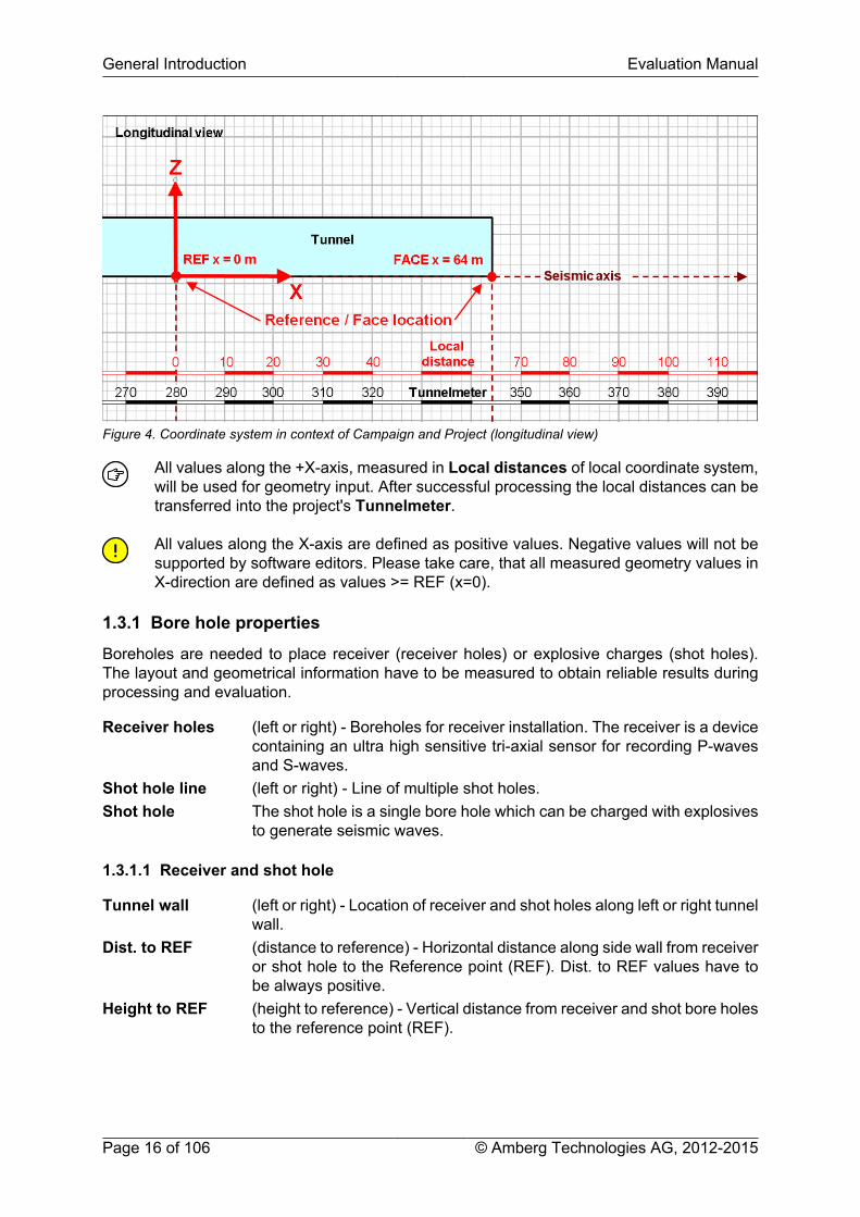
Figure 4. Coordinate system in context of Campaign and Project (longitudinal view)
All values along the +X-axis, measured in Local distances of local coordinate system,will be used for geometry input. After successful processing the local distances can betransferred into the project's Tunnelmeter.
All values along the X-axis are defined as positive values. Negative values will not besupported by software editors. Please take care, that all measured geometry values inX-direction are defined as values >= REF (x=0).
1.3.1 Bore hole properties
Boreholes are needed to place receiver (receiver holes) or explosive charges (shot holes).The layout and geometrical information have to be measured to obtain reliable results duringprocessing and evaluation.
Receiver holes (left or right) - Boreholes for receiver installation. The receiver is a devicecontaining an ultra high sensitive tri-axial sensor for recording P-wavesand S-waves.
Shot hole line (left or right) - Line of multiple shot holes.Shot hole The shot hole is a single bore hole which can be charged with explosives
to generate seismic waves.
1.3.1.1 Receiver and shot hole
Tunnel wall (left or right) - Location of receiver and shot holes along left or right tunnelwall.
Dist. to REF (distance to reference) - Horizontal distance along side wall from receiveror shot hole to the Reference point (REF). Dist. to REF values have tobe always positive.
Height to REF (height to reference) - Vertical distance from receiver and shot bore holesto the reference point (REF).

Evaluation Manual General Introduction
© Amberg Technologies AG, 2012-2015 Page 17 of 106
Figure 5. Receiver and shot hole properties (longitudinal view)
Depth Depth of tri-axial sensors or explosive charge. The depth values may beless than the drilled bore hole depth for receiver and shot holes dependingon depth accessibility. Depth values are measured always as positivevalues. Amberg TSP Plus software will assign depth values to selectedtunnel wall.
Vertical angle Upward or downward inclination of boreholes. Upward inclination is pos-itive and downward inclination is negative. This convention is valid for leftand right tunnel wall.
Inclination angles range from -90° to +90°.
Figure 6. Vertical angles of boreholes (profile view)
Horizontal angle The angle is defined as the horizontal deviation of boreholes from theperpendicular to the Reference axis in the horizontal plane. If the borehole deviates toward the Face, the angle is positive. In other case, theangle is negative.
Horizontal angles range from -90° to +90°.
General Introduction Evaluation Manual
Page 18 of 106 © Amberg Technologies AG, 2012-2015
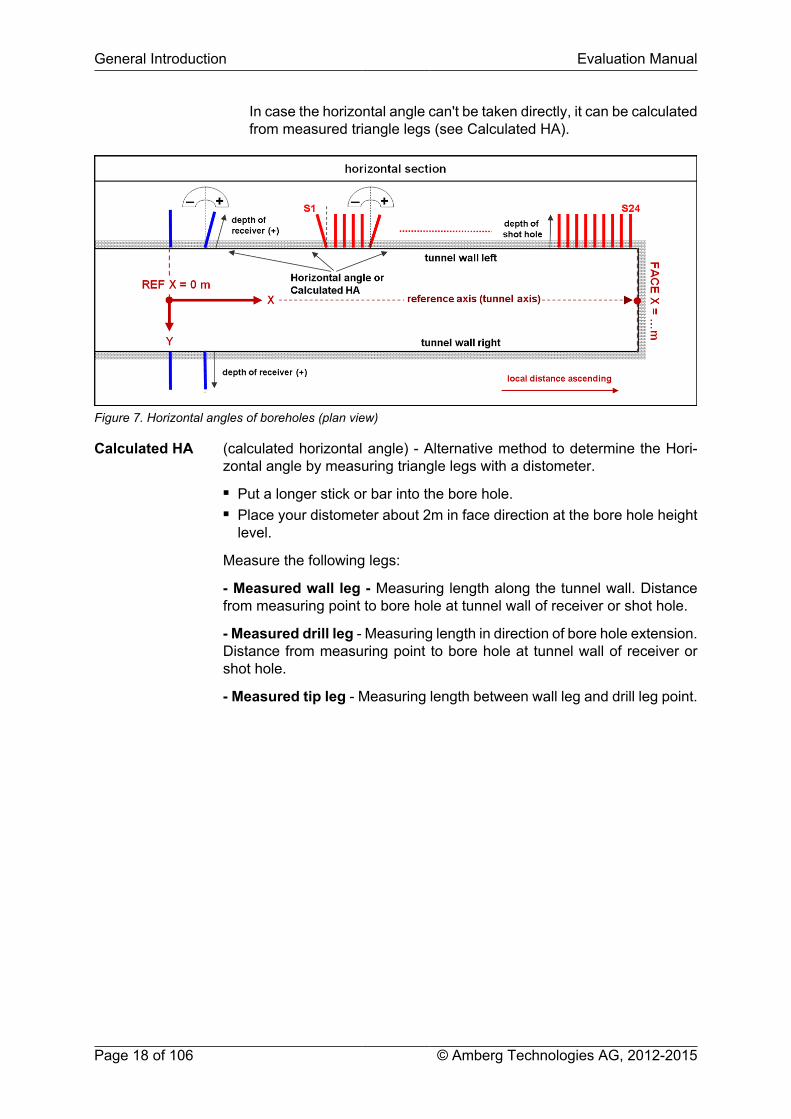
In case the horizontal angle can't be taken directly, it can be calculatedfrom measured triangle legs (see Calculated HA).
Figure 7. Horizontal angles of boreholes (plan view)
Calculated HA (calculated horizontal angle) - Alternative method to determine the Hori-zontal angle by measuring triangle legs with a distometer.■ Put a longer stick or bar into the bore hole.■ Place your distometer about 2m in face direction at the bore hole height
level.
Measure the following legs:
- Measured wall leg - Measuring length along the tunnel wall. Distancefrom measuring point to bore hole at tunnel wall of receiver or shot hole.
- Measured drill leg - Measuring length in direction of bore hole extension.Distance from measuring point to bore hole at tunnel wall of receiver orshot hole.
- Measured tip leg - Measuring length between wall leg and drill leg point.

Evaluation Manual General Introduction
© Amberg Technologies AG, 2012-2015 Page 19 of 106
Figure 8. Calculated HA of boreholes (plan view)
Twist angle Angle of rotation around the receiver's longitudinal axis. If the longitudinal axisof the receiver is twisted towards the Face, the twist angle is positive. In theother case it is negative.
Twist angle range from -180° to +180°.
Figure 9. Twist angle of receiver at tunnel wall left and right

General Introduction Evaluation Manual
Page 20 of 106 © Amberg Technologies AG, 2012-2015
1.4 Description of the work space
Figure 10. Work space
Menu bar (1): Start of software the base menus are available. Depending on the opened /selected editor additional menus may appear.
Toolbars (2): Start the software the base toolbars are available. The base toolbar consistsof frequently performed operations such as opening and saving projects, tiling and cascadingwindows, adding and deleting items in currently active editor, zooming and panning. Dependingon the opened / selected editor additional editor specific toolbars may appear.
Project tree window (3): Once a project is opened or created, the project tree window showsthe project structure. All relevant functions to add or remove campaigns to/from the project ordo specific editing and processing in the campaigns can be reached through context menus(right-click on tree node).
Property window (4): The property window shows properties of the currently selected elementin the project tree. Certain properties can be edited after an element has been created andothers are read only.
Seismic view & Editor window (5): The content of seismic views and editors depends on theview or editor type. In case the editor title starts with an asterisk (*) the editor contains unsaveddata. Depending on the viewer type, an additional Option window (8) may appear.

Evaluation Manual General Introduction
© Amberg Technologies AG, 2012-2015 Page 21 of 106
Processing monitor window (6): The processing monitor window shows the data processingflow chart of a currently selected campaign. Every node represents a processing step that canbe individually edited and processed. Results of single processing steps can be displayed inthe Seismic view (5).
Spectrum or Histogram Window (7): The Spectrum window shows the frequency content ofthe corresponding data in the seismic trace view. The Histogram window shows the densityplot of the velocity or reflectivity distribution of the corresponding data in the 3D view.
Option window (8): This window is dependent on the viewer type. View settings can be setindividually to optimize appearance of the viewer content.
1.4.1 Customizing workspace components
Docking windows (all windows besides the Seismic view editor (5)) can be activated and de-activated by invoking corresponding item in View menu or context menu on the right side oftoolbars. They can be closed by window controlling buttons in top-right corner of each dockingwindow as well.
Toolbars can be switched on/off by right-clicking in the base menu bar and selecting menu itemof common actions or editor specific actions.
The status bar can be hidden or restored by selecting View ▶ Status bar menu item.
All docking windows can be rearranged freely by drag and drop operations on their title bar.
1.5 General menu functionsAfter starting up Amberg TSP Plus the following menus are available. Additional menus mayappear depending on currently activated editor or views.
1.5.1 Menu File
New project... Opens the New project wizard which supports the user in creating anew Amberg TSP Plus project.
Open project... Shows a file open dialog to browse for an existing project file and openit. Amberg TSP Plus projects have the file extension *.tsp3prj.
Note that all Amberg TSP Plus project files are directly linked tothe software installation. It is therefore possible to open a projectby double-clicking on the project file in the Windows file explorer.
The project tree state is stored for every project when closing the Am-berg TSP Plus software respectively when opening another project.When opening a project again, the tree state will be the same as whenleaving the project.
Save Saves all modifications of the active editor.Save all Saves all modifications of all editors.Recent projects Shows a list of recently used projects in Amberg TSP Plus. Click on the
displayed file path to open a recent project.Options... Opens the Options dialog.Exit Closes the program. If there is unsaved data the program asks for saving
before closing the program.

General Introduction Evaluation Manual
Page 22 of 106 © Amberg Technologies AG, 2012-2015
1.5.2 Menu View
Project tree Switches on / off the project tree window.Property window Switches on / off the property window.Processing monitor Switches on / off the processing monitor.Status bar Switches on / off the status bar.
1.5.3 Menu Window
Cascade Cascades all currently opened windows in the working space.Tile horizontally Tiles all currently opened windows horizontally.Tile vertically Tiles all currently opened windows vertically.Close all windows Closes all currently opened windows in the working space.
1.5.4 Menu Help
Help - Amberg TSP Plus Eval-uation, Help - TSP 303 PlusOperation
Opens the Amberg TSP Plus Evaluation and TSP 303 Plusoperation help files.
Licence tool... Opens the licence viewer. In the case dongles are connect-ed, dongle ID and stored licence information are shown. Li-cences upgrades only can be done by exchange of licencefiles between client to vendor (c2v) represented by AmbergTechnologies AG and back from vendor to client (v2c).
Update key from v2c file ...- In case you received licenceupgrade file (v2c) from Amberg Technologies AG updateyour licence by importing the v2c file to the correspondingdongle key. The new licence will be stored on the corre-sponding dongle.
Refresh key data - Refresh the view of dongle key andlicence information.
Create 123456.c2v file... - In case you need to upgradeyour licence, create a c2v file from corresponding donglekey and send the exported file to Amberg Technologies AG.
About Amberg TSP Plus... Shows a dialog with general information about software ver-sion, dongle serial number, licensed modules and softwarecomponents.
1.6 General toolbarThe general toolbar allows you to perform actions, which are related to all views and editors
Depending on functionality of opened windows, views and editors the toolbar buttonsmay be deactivated.
Figure 11. General toolbar

Evaluation Manual General Introduction
© Amberg Technologies AG, 2012-2015 Page 23 of 106
Open project opens the project file.
Save the current editor.
Save all unsaved data at once.
Cascade organises windows in cascade pattern.
Tile horizontally tiles opened editors windows horizontally.
Tile vertically tiles opened editors vertically.
Add new item to currently active editor.
Delete the current item.
Drag on graphic zooms by rectangle.
Pan view by mouse dragging.
Zoom in opened view.
Zoom out opened view.
Zoom to show all displayed objects.
Top view of 3D visualisation.
Front view of 3D visualisation.
Side view of 3D visualisation.
Reset 3D position.
3D navigation cross on/off.
1.7 Program optionsThe Options dialog in the File menu contains the main option sections - General and Prefer-ences.
1.7.1 General - Labels
Software owner and Operator name information can be edited here as sender address. Theinformation is displayed in the footer and header of the reports as Report creator.

General Introduction Evaluation Manual
Page 24 of 106 © Amberg Technologies AG, 2012-2015
Figure 12. Options dialog - Labels
If no entries are made in the software owner fields, the Amberg Technologies contactdetails including logo are presented in reports.
If you like to have presented your own details, even only the logo, the field entry inCompany name is compulsory.
1.7.2 Graphics
Grid color settings for 2D- and 3D-views can be set here.
Figure 13. Options dialog - Graphics
1.7.3 Preferences - Language
Language for the user interface and the reporting can be set here.

Evaluation Manual General Introduction
© Amberg Technologies AG, 2012-2015 Page 25 of 106
Figure 14. Options dialog - Language
User interface language Sets the language, which is used for the software user inter-face.
Reporting language Sets a separate language for all the reports created in Am-berg TSP Plus. The reporting language may be different fromthe user interface language.
Access to languages may depend on available license.
1.7.4 Preferences - Units
Units, formats and number of decimals in table and graphic views for different value types canbe customized here.
Figure 15. Options dialog - Units
Units and formatting for the following categories can be set:

General Introduction Evaluation Manual
Page 26 of 106 © Amberg Technologies AG, 2012-2015
Tunnelmeter used for stationing in Tunnelmeter.Local distances used for local coordinate system referenced to the Reference point REF.Velocity used for seismic velocity values.Frequency used for seismic wave frequency values.Angles used for all measured angles such as vertical, horizontal and twist an-
gles as well as for processed angles like strike and dip angles.Modulus used for compressive strength, dyn. and stat. Young's modulus, Bulk
modulus and Shear modulus.Density used for rock densities.Voltage used for all magnitudes of seismic signals.Charge used for all shot hole charge sizes, e.g. for explosive charge sizeTime window used for time values such as time scaling in views and time parameters
for processing .
Import and export of unit options
Unit and format options can be exported to an xml file to share them between workstations.Press the Export... button and export the options file to the specified location. To import optionsagain, press the Import... button and select the options file in the dialog.
1.8 ShortcutsCtrl + N New Project...Ctrl + O Open project...Ctrl + S Save editorCtrl + C Copy selected input field content to clipboardCtrl + V Paste clipboard content to selected input fieldCtrl + A Select all content of a input field or tableCtrl + ↑ / ↓ Zoom in/out time axisCtrl + ← / → Zoom out/in offset axisCtrl + Scroll mouse wheel Zoom in/out time axisShift + Scroll mouse wheel Zoom in/out offset axisShift + left mouse button Pan 3D objectCtrl + left mouse button Rotation of 3D object around focal pointX,Y or Z select / unselect rotation axis in 3D viewsTAB Navigate forward through input forms and table cellsShift + TAB Navigate backward through input forms and table cells← / → Navigate backward/forward through input forms and table
cells↑ / ↓ Navigate upward/downward through input forms and table
cells
Evaluation Manual
© Amberg Technologies AG, 2012-2015 Page 27 of 106
Chapter 2 Getting started2.1 ProjectA Project is a folder managing all tunnel related data and files suitable for tunnel seismic pre-diction. For every new tunnel project an own project folder is recommended.
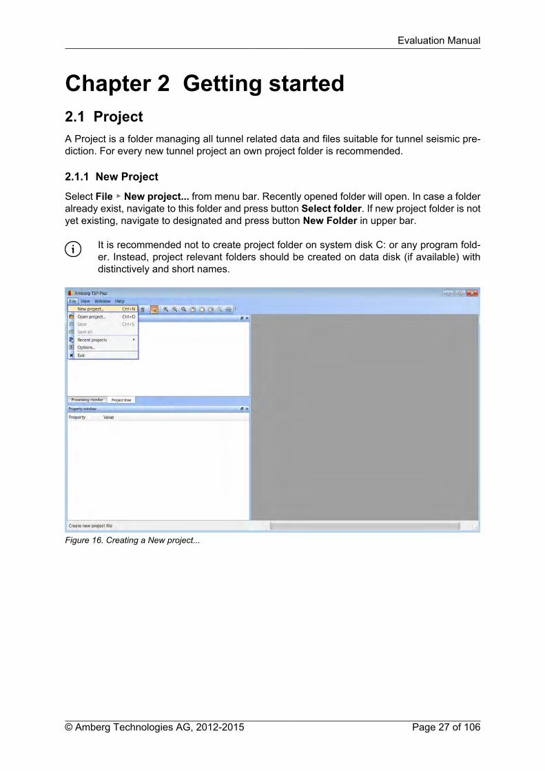
2.1.1 New Project
Select File ▶ New project... from menu bar. Recently opened folder will open. In case a folderalready exist, navigate to this folder and press button Select folder. If new project folder is notyet existing, navigate to designated and press button New Folder in upper bar.
It is recommended not to create project folder on system disk C: or any program fold-er. Instead, project relevant folders should be created on data disk (if available) withdistinctively and short names.
Figure 16. Creating a New project...

Getting started Evaluation Manual
Page 28 of 106 © Amberg Technologies AG, 2012-2015
Figure 17. Selection of project folder
After the folder for the new project is selected, the project will be shown with its selected foldername and the base structure of the Project tree. The Property Window offers the possibility torename the name of project if necessary. Additionally, the clients address can be added here.

Evaluation Manual Getting started
© Amberg Technologies AG, 2012-2015 Page 29 of 106
Figure 18. Property window Project...
2.2 The TSP Project TreeThe Project tree structure and its subtree elements with its wizards and editors reflects the workflow of tunnel seismic predictions within the whole tunnel project. Mainly, the subsequent levelnode need completion of previous level node.
Figure 19. Project tree structure
First level node Project and Property window with project relevant informationsuch as project name and address of recipient.

Getting started Evaluation Manual
Page 30 of 106 © Amberg Technologies AG, 2012-2015
Second level nodes A Rock catalogue editor for definition of project dominant rockgroups and rock types in the project is available. Campaigns is theregister of all performed seismic measurement in the project.
Third level nodes Campaign and Property window with campaign relevant informa-tion such as Campaign name, Survey date, Face location, station-ing direction and overburden have to be defined.
Fourth level nodes From the campaign level node, access to all subsequent work flowsteps is given, as there are Acquisition, Shot data, Geometry andData processing.
Fifth level nodes From the Geometry node there is access to Profiles, Tunnel mod-el and Receiver / Shot hole lines editors which allow to imagethe excavated tunnel and to map the seismic layout. From the Dataprocessing node a processing instance with its Property windowwith processing relevant information such as processing name andmodification dates is added.
Sixth level nodes Access to Survey Setup, Processing Monitor, and Evaluation seteditors were selection of seismic traces, the data processing anddata evaluation can be done.
2.3 Rock CatalogueOnce a new project is created, the Rock Catalogue is available. The rock catalogue is a projectrelated database and contains most dominant rock groups, rock types and their properties. Youcan edit and add rock information.
The Rock Catalogue editor can be opened with a double click on the node or with the contextmenu "Edit rock catalogue".
Figure 20. Rock catalogue editor
Evaluation Manual Getting started
© Amberg Technologies AG, 2012-2015 Page 31 of 106
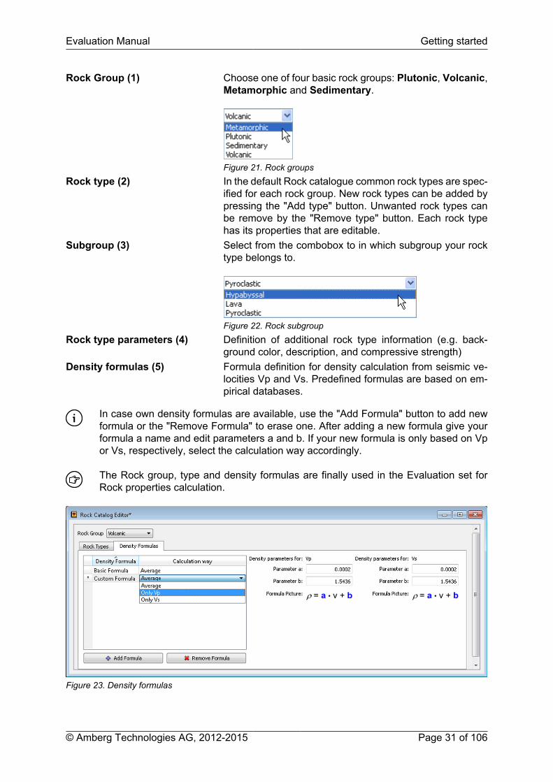
Rock Group (1) Choose one of four basic rock groups: Plutonic, Volcanic,Metamorphic and Sedimentary.
Figure 21. Rock groupsRock type (2) In the default Rock catalogue common rock types are spec-
ified for each rock group. New rock types can be added bypressing the "Add type" button. Unwanted rock types canbe remove by the "Remove type" button. Each rock typehas its properties that are editable.
Subgroup (3) Select from the combobox to in which subgroup your rocktype belongs to.
Figure 22. Rock subgroupRock type parameters (4) Definition of additional rock type information (e.g. back-
ground color, description, and compressive strength)Density formulas (5) Formula definition for density calculation from seismic ve-
locities Vp and Vs. Predefined formulas are based on em-pirical databases.
In case own density formulas are available, use the "Add Formula" button to add newformula or the "Remove Formula" to erase one. After adding a new formula give yourformula a name and edit parameters a and b. If your new formula is only based on Vpor Vs, respectively, select the calculation way accordingly.
The Rock group, type and density formulas are finally used in the Evaluation set forRock properties calculation.
Figure 23. Density formulas

Getting started Evaluation Manual
Page 32 of 106 © Amberg Technologies AG, 2012-2015
2.4 CampaignThe node Campaign and its sub nodes consisting of wizards and editors do organize the workflow and order of actions of data acquisition, geometry input and data processing includingevaluation.
In case of new data acquisition, firstly a campaign needs to be added to the project. New dataacquisition or additional data acquisitions can be done in all listed campaigns. The Add/Deletecampaign functionalities enable managing data content in the existing project. The Export andImport campaign support the data exchange between construction site and office. It reducescampaign data content to a minimum of necessary information which can be transferred fastand easily. The exported files contain all information for rebuilding and reprocessing origincampaign content.
Figure 24. New campaign....
2.4.1 Add Campaign...
To add a new campaign, right-click on the Campaigns node in the Project tree and selectAdd Campaign from the pop-up menu.
Figure 25. Add campaign....
After adding, an "Add campaign..." wizard opens to specify campaign related informationand data.

Evaluation Manual Getting started
© Amberg Technologies AG, 2012-2015 Page 33 of 106
Figure 26. Add campaign wizard....
All input in the Add campaign wizard should be edited carefully and checked beforepressing OK. All edited values will be used to identify the campaign and settings areused for later processing.
Name Definition of the campaign's name.Survey date Date of data acquisition. Default is date of campaign creation.
Should be set to date of acquisition if it is different.Operator Definition of Operator's name.Tunnelmeter referencing Referencing the campaign in tunnelmeter at date of acquisi-
tion based on Face location or REF point location. Needs tobe defined to reference the campaign to the tunnel station-ing. Editing tunnelmeter at date of acquisition.
Face direction Definition of excavation direction in relation to stationing di-rection.
Overburden Value of overburden at face location. Value is used for cal-culation of overburden dependent statical Young's modulusin Evaluation set.
All information edited in the Add campaign wizard are shown in the Campaign's propertywindow. In case of wrong or missing values, the property window allows to edit relevant cellslater on.

Getting started Evaluation Manual
Page 34 of 106 © Amberg Technologies AG, 2012-2015
Figure 27. Property window Campaign...
2.4.2 Import campaign...
The Import campaign... inserts from Amberg TSP Plus exported archive file into the currentlyopened project tree.
Figure 28. Import campaign....
After selection of *.zip archive, an "Import wizard" opens with Archive and Import information.
Evaluation Manual Getting started
© Amberg Technologies AG, 2012-2015 Page 35 of 106
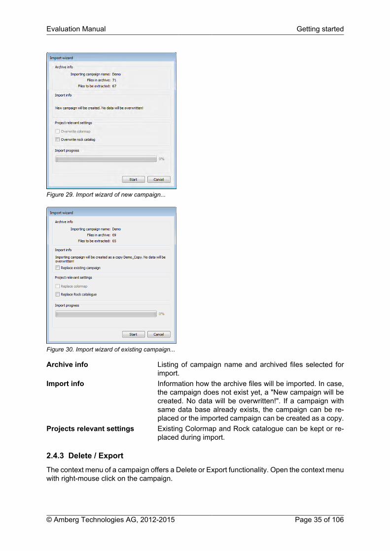
Figure 29. Import wizard of new campaign...
Figure 30. Import wizard of existing campaign...
Archive info Listing of campaign name and archived files selected forimport.
Import info Information how the archive files will be imported. In case,the campaign does not exist yet, a "New campaign will becreated. No data will be overwritten!". If a campaign withsame data base already exists, the campaign can be re-placed or the imported campaign can be created as a copy.
Projects relevant settings Existing Colormap and Rock catalogue can be kept or re-placed during import.
2.4.3 Delete / Export
The context menu of a campaign offers a Delete or Export functionality. Open the context menuwith right-mouse click on the campaign.

Getting started Evaluation Manual
Page 36 of 106 © Amberg Technologies AG, 2012-2015
Delete The option deletes all campaign relevant information and data, including all subtreesnodes with acquisition, geometry, processing and evaluation.
Export All project information and the selected campaign will be exported to a zip-file withminimum data volume which is necessary to rebuild the information after unzip.
Delete functionality will empty all campaign relevant information, data and results fromproject. The loss of data will be accepted by user.
The export functionality can be used for exchange of data between different worksta-tions or for email transfer.
Figure 31. Delete / Export functionality of campaign
2.5 AcquisitionThe Acquisition wizard will guide the user through data recording. The wizard allows the user todefine relevant receiver and shot information on time before or after acquired shot. For detailedinformation refer to the TSP 303 PLUS Operation Manual.
The wizard can be opened with right-click in the context menu of Acquisition ▶ Open... or witha double click on Acquisition node.
Access to acquisition wizard is only possible when the recording unit is connected andswitched on.
Figure 32. Open Acquisition wizard
2.6 Shot dataAfter a successful data acquisition, shot information can be viewed in the Shot data editor.

Evaluation Manual Getting started
© Amberg Technologies AG, 2012-2015 Page 37 of 106
Figure 33. Shot data editor
Shot data table (1) This table allows Shot No. to Shot hole line No. and Shot holeassignment, organizing the shot data and their shot hole loca-tions. Shots which should be kept/not kept for further processingcan be activated/deactivated in Status column. The used Chargesize can be controlled and edited. The recording time of each shotis listed in the column Time showing the local time of computer.The value of maximum magnitude of a shot is listed in the columnMagn. Further Remarks for each shot can be edited, if additionalinformation are important for processing.
Figure 34. Header of Shot data editor
Shot data view (2) This view shows the raw shot data. The data can be visualized insingle shot view or component view style. The shot view showssingle shot data of all connected receivers and their components(X, Y, Z). It should be used for seismic data control. The componentview shows a gather of all recorded shots per selected component.Selection and seismic display settings are controlled in the windowof seismic view options (3).

Getting started Evaluation Manual
Page 38 of 106 © Amberg Technologies AG, 2012-2015
Figure 35. Data view of Shot data editor with different axis labelling
Seismic view options (3) Option window with settings for seismic trace displaying.
2.6.1 Shot data toolbar
Figure 36. Shot data toolbar
Reload content of current editor
Zoom in/out time axis
Zoom in/out offset axis
Show value function. After activation click on a trace in seismic trace view. At nodeposition trace information of magnitude, time and offset are shown.
Show time range function. After activation click on a trace in seismic trace view. Atime range window shows time range between beginning point and cursor position.
Open Seismic view option window
2.6.2 Shot data display options
The shot data display option is assigned to opened shot data windows. The option windowopens automatically by double click on Shot data node.

Evaluation Manual Getting started
© Amberg Technologies AG, 2012-2015 Page 39 of 106
Object selectorControl of view selection between Shotview and Component view. Componentsselector becomes active, if componentview is selectedTrace styleVariable area shows trace in polarity col-ors (red: positive, blue: negative).
Wiggles shows seismic traces without po-larity coloring.
Show axes activates / deactivates the vi-sualisation of the trace base line.
Trace normalizationTrace normalization normalises eachtrace by its maximum amplitude. Crossnormalization normalises all traces bymaximum amplitude of entire data set. Au-tomatic gain control is a window-length-weighted normalization to let weaker sig-nals receive more gain and stronger sig-nals receiver less or none gain.Amplitude gainGain defines the gain factor of signalamplitude. The visualization of overlap-ping traces can be activated/deactivatedby Clipping.InformationNot available for Shot data view
2.7 GeometryIn the Geometry node seismic layout relevant editors will be available for editing Profiles,Tunnel model and Receiver / Shot hole lines. In these editors, campaign specific geometricinformation of the tunnel and the survey points of receivers and shots have to be defined. Theeditors allow to image the tunnel and seismic layout between Reference point (REF) and tunnelface as realistic as possible.
The editors are modular based composed and depend on each other. It is recommended toedit geometry in following steps:
Getting started Evaluation Manual
Page 40 of 106 © Amberg Technologies AG, 2012-2015
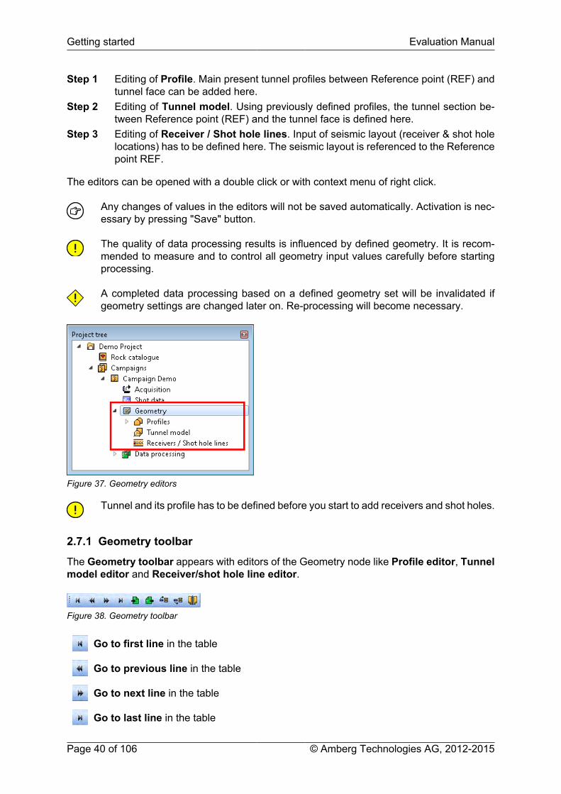
Step 1 Editing of Profile. Main present tunnel profiles between Reference point (REF) andtunnel face can be added here.
Step 2 Editing of Tunnel model. Using previously defined profiles, the tunnel section be-tween Reference point (REF) and the tunnel face is defined here.
Step 3 Editing of Receiver / Shot hole lines. Input of seismic layout (receiver & shot holelocations) has to be defined here. The seismic layout is referenced to the Referencepoint REF.
The editors can be opened with a double click or with context menu of right click.
Any changes of values in the editors will not be saved automatically. Activation is nec-essary by pressing "Save" button.
The quality of data processing results is influenced by defined geometry. It is recom-mended to measure and to control all geometry input values carefully before startingprocessing.
A completed data processing based on a defined geometry set will be invalidated ifgeometry settings are changed later on. Re-processing will become necessary.
Figure 37. Geometry editors
Tunnel and its profile has to be defined before you start to add receivers and shot holes.
2.7.1 Geometry toolbar
The Geometry toolbar appears with editors of the Geometry node like Profile editor, Tunnelmodel editor and Receiver/shot hole line editor.
Figure 38. Geometry toolbar
Go to first line in the table
Go to previous line in the table
Go to next line in the table
Go to last line in the table

Evaluation Manual Getting started
© Amberg Technologies AG, 2012-2015 Page 41 of 106
Import profile from *.dxf file
Export profile to *.dxf file
Insert element before current line
Insert element after current line
Mirror current elements
2.8 ProfileA single profile or multiple profiles can be used to model the tunnel situation. If excavation isdone with TBM, e.g. only one profile is necessary to model the excavated tunnel diameter. Indrill and bast headings the excavated tunnel profile may vary between Reference point andtunnel face. Examples could be top heading, niches left or right, etc. In this case, several profilesare necessary to model the tunnel situation.
There are two default profiles in each new campaign (Default profile TBM, Default profileD&B). The Default profile TBM is used as default profile for acquisition.
2.8.1 Add profile
To add a new profile, right-click on Profiles node in Project tree.
Figure 39. Add profile...
Define the profile properties in the shown dialog. Edit a Name representing the profiles appear-ance. Type in a Comment which may help other users to identify the profile. Confirm with OKand the new profile will appear as a sub-node in the tree.
Figure 40. Profile properties...
Getting started Evaluation Manual
Page 42 of 106 © Amberg Technologies AG, 2012-2015
2.8.2 Edit profile
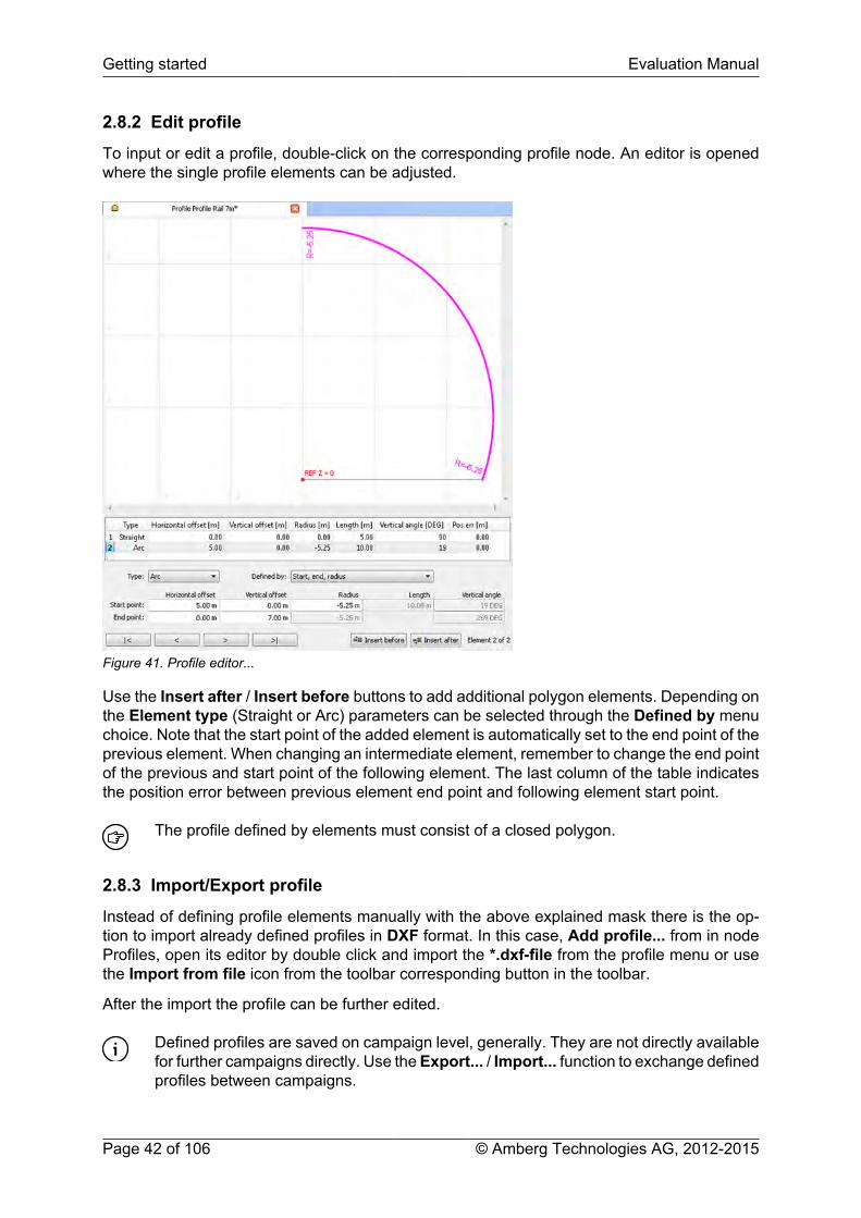
To input or edit a profile, double-click on the corresponding profile node. An editor is openedwhere the single profile elements can be adjusted.
Figure 41. Profile editor...
Use the Insert after / Insert before buttons to add additional polygon elements. Depending onthe Element type (Straight or Arc) parameters can be selected through the Defined by menuchoice. Note that the start point of the added element is automatically set to the end point of theprevious element. When changing an intermediate element, remember to change the end pointof the previous and start point of the following element. The last column of the table indicatesthe position error between previous element end point and following element start point.
The profile defined by elements must consist of a closed polygon.
2.8.3 Import/Export profile
Instead of defining profile elements manually with the above explained mask there is the op-tion to import already defined profiles in DXF format. In this case, Add profile... from in nodeProfiles, open its editor by double click and import the *.dxf-file from the profile menu or usethe Import from file icon from the toolbar corresponding button in the toolbar.
After the import the profile can be further edited.
Defined profiles are saved on campaign level, generally. They are not directly availablefor further campaigns directly. Use the Export... / Import... function to exchange definedprofiles between campaigns.
Evaluation Manual Getting started
© Amberg Technologies AG, 2012-2015 Page 43 of 106
Try to image tunnel profiles as realistic as possible. Wrong profiling reduces the accu-racy of further seismic waves processing.
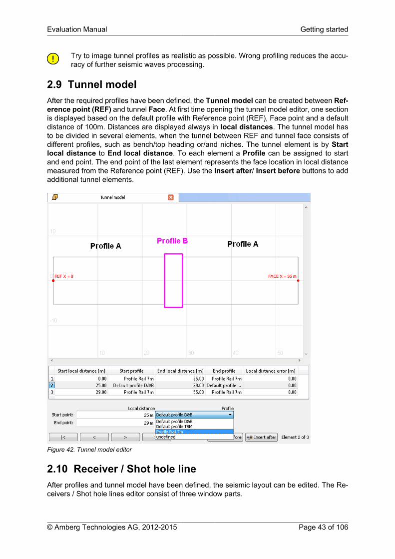
2.9 Tunnel modelAfter the required profiles have been defined, the Tunnel model can be created between Ref-erence point (REF) and tunnel Face. At first time opening the tunnel model editor, one sectionis displayed based on the default profile with Reference point (REF), Face point and a defaultdistance of 100m. Distances are displayed always in local distances. The tunnel model hasto be divided in several elements, when the tunnel between REF and tunnel face consists ofdifferent profiles, such as bench/top heading or/and niches. The tunnel element is by Startlocal distance to End local distance. To each element a Profile can be assigned to startand end point. The end point of the last element represents the face location in local distancemeasured from the Reference point (REF). Use the Insert after/ Insert before buttons to addadditional tunnel elements.
Figure 42. Tunnel model editor
2.10 Receiver / Shot hole lineAfter profiles and tunnel model have been defined, the seismic layout can be edited. The Re-ceivers / Shot hole lines editor consist of three window parts.

Getting started Evaluation Manual
Page 44 of 106 © Amberg Technologies AG, 2012-2015
Receivers / Shot hole lineseditor (1)
Editor tables of Receivers and Shot hole lines with proper-ties of receivers, shot lines and shot holes.
General view of locations (2) Longitudinal and plan views of Receivers and Shot holelines locations, seismic axis, Reference point (REF), Facelocation and tunnel model. All values are given in Local dis-tances.
Perspective view of locations(3)
Perspective view of Receivers and Shot hole lines loca-tions, seismic axis and tunnel model. All values are given inLocal distances. Coordinate system (X,Y,Z) is indicated.
Receivers / Shot hole lines settings are directly linked to the Acquisition wizard. Alllisted Receivers and Shot hole lines with defined Shot holes are selectable during theacquisition. Vice versa, all Receivers, Shot hole lines and Shot holes which were definedin the Acquisition wizard will be listed in the geometry tables.
Complex tunnel models can be checked in the longitudinal, plan and perspective views.Here in particular, check used Start and End profiles of respective tunnel elements.
Figure 43. Receivers / Shot hole lines editor
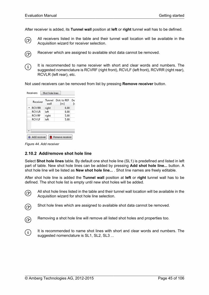
2.10.1 Add/remove receiver
Select the Receivers table. By default two receivers (RCV1 and RCV2) are predefined andlisted in left part of table. New receiver can be added by pressing Add Receiver... button. ANew receiver... is listed and can be renamed.
Evaluation Manual Getting started
© Amberg Technologies AG, 2012-2015 Page 45 of 106
After receiver is added, its Tunnel wall position at left or right tunnel wall has to be defined.
All receivers listed in the table and their tunnel wall location will be available in theAcquisition wizard for receiver selection.
Receiver which are assigned to available shot data cannot be removed.
It is recommended to name receiver with short and clear words and numbers. Thesuggested nomenclature is RCVRF (right front), RCVLF (left front), RCVRR (right rear),RCVLR (left rear), etc.
Not used receivers can be removed from list by pressing Remove receiver button.
Figure 44. Add receiver
2.10.2 Add/remove shot hole line
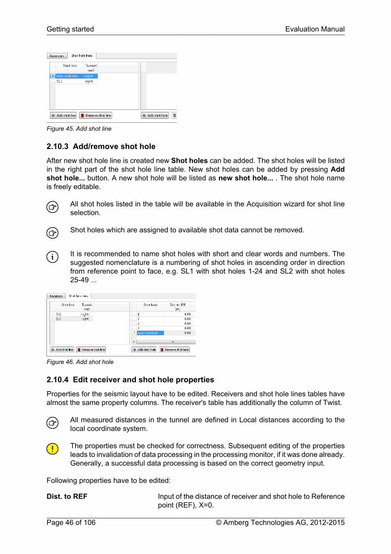
Select Shot hole lines table. By default one shot hole line (SL1) is predefined and listed in leftpart of table. New shot hole lines can be added by pressing Add shot hole line... button. Ashot hole line will be listed as New shot hole line... . Shot line names are freely editable.
After shot hole line is added the Tunnel wall position at left or right tunnel wall has to bedefined. The shot hole list is empty until new shot holes will be added.
All shot hole lines listed in the table and their tunnel wall location will be available in theAcquisition wizard for shot hole line selection.
Shot hole lines which are assigned to available shot data cannot be removed.
Removing a shot hole line will remove all listed shot holes and properties too.
It is recommended to name shot lines with short and clear words and numbers. Thesuggested nomenclature is SL1, SL2, SL3 ...
Getting started Evaluation Manual
Page 46 of 106 © Amberg Technologies AG, 2012-2015
Figure 45. Add shot line
2.10.3 Add/remove shot hole
After new shot hole line is created new Shot holes can be added. The shot holes will be listedin the right part of the shot hole line table. New shot holes can be added by pressing Addshot hole... button. A new shot hole will be listed as new shot hole... . The shot hole nameis freely editable.
All shot holes listed in the table will be available in the Acquisition wizard for shot lineselection.
Shot holes which are assigned to available shot data cannot be removed.
It is recommended to name shot holes with short and clear words and numbers. Thesuggested nomenclature is a numbering of shot holes in ascending order in directionfrom reference point to face, e.g. SL1 with shot holes 1-24 and SL2 with shot holes25-49 ...
Figure 46. Add shot hole
2.10.4 Edit receiver and shot hole properties
Properties for the seismic layout have to be edited. Receivers and shot hole lines tables havealmost the same property columns. The receiver's table has additionally the column of Twist.
All measured distances in the tunnel are defined in Local distances according to thelocal coordinate system.
The properties must be checked for correctness. Subsequent editing of the propertiesleads to invalidation of data processing in the processing monitor, if it was done already.Generally, a successful data processing is based on the correct geometry input.
Following properties have to be edited:
Dist. to REF Input of the distance of receiver and shot hole to Referencepoint (REF), X=0.
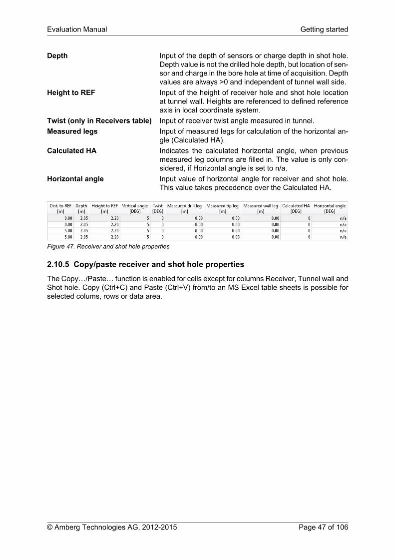
Evaluation Manual Getting started
© Amberg Technologies AG, 2012-2015 Page 47 of 106
Depth Input of the depth of sensors or charge depth in shot hole.Depth value is not the drilled hole depth, but location of sen-sor and charge in the bore hole at time of acquisition. Depthvalues are always >0 and independent of tunnel wall side.
Height to REF Input of the height of receiver hole and shot hole locationat tunnel wall. Heights are referenced to defined referenceaxis in local coordinate system.
Twist (only in Receivers table) Input of receiver twist angle measured in tunnel.Measured legs Input of measured legs for calculation of the horizontal an-
gle (Calculated HA).Calculated HA Indicates the calculated horizontal angle, when previous
measured leg columns are filled in. The value is only con-sidered, if Horizontal angle is set to n/a.
Horizontal angle Input value of horizontal angle for receiver and shot hole.This value takes precedence over the Calculated HA.
Figure 47. Receiver and shot hole properties
2.10.5 Copy/paste receiver and shot hole properties
The Copy…/Paste… function is enabled for cells except for columns Receiver, Tunnel wall andShot hole. Copy (Ctrl+C) and Paste (Ctrl+V) from/to an MS Excel table sheets is possible forselected colums, rows or data area.

Getting started Evaluation Manual
Page 48 of 106 © Amberg Technologies AG, 2012-2015
Figure 48. Copy/Paste receiver and shot hole properties
2.11 Data processingAfter acquisition and geometry input, the processing of data can be started. The sub node ofData Processing allows individual Processing of data. The processing offers three editors forsophisticated data processing.
Survey setup Seismic trace view of rawdata with editor for data quality check. Pres-election of traces to be used for processing is possible.
Processing setup User-leading processing monitor with editors of processing parame-ters. Option of seismic trace views and volume views, respectively ofeach processing step.
Evaluation set Editor for evaluation and interpretation of processing results. Tablewith calculated rock properties based on processing results. Prepara-tion of result report.

Evaluation Manual Getting started
© Amberg Technologies AG, 2012-2015 Page 49 of 106
Figure 49. Data processing node
2.11.1 Add processing
To add an individual processing, right-click on the Data Processing node in the Project treeand select Add Processing from the context menu.
Figure 50. Add processing....
After adding, a property window appears and an individual processing name can be defined.
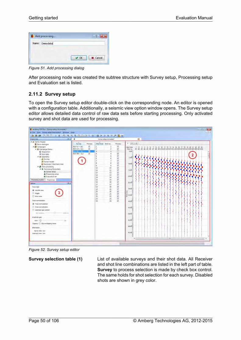
Getting started Evaluation Manual
Page 50 of 106 © Amberg Technologies AG, 2012-2015
Figure 51. Add processing dialog
After processing node was created the subtree structure with Survey setup, Processing setupand Evaluation set is listed.
2.11.2 Survey setup
To open the Survey setup editor double-click on the corresponding node. An editor is openedwith a configuration table. Additionally, a seismic view option window opens. The Survey setupeditor allows detailed data control of raw data sets before starting processing. Only activatedsurvey and shot data are used for processing.
Figure 52. Survey setup editor
Survey selection table (1) List of available surveys and their shot data. All Receiverand shot line combinations are listed in the left part of table.Survey to process selection is made by check box control.The same holds for shot selection for each survey. Disabledshots are shown in grey color.

Evaluation Manual Getting started
© Amberg Technologies AG, 2012-2015 Page 51 of 106
Figure 53. Survey setup table for preselection of surveys and shot data to be used in processing
Seismic trace view (2) Display of seismic traces depending on selected survey. Ac-tive shots data are colored red/blue and inactive shots are col-ored grey. Upper labeling of horizontal axis shows Shot holeno. while lower shows Shot no. according to ascending offsetfrom left to right..
Figure 54. Seismic trace view of Survey setup editor (greyed trace is notused in processing)
Seismic view options (3) Option window with settings for individual seismic trace dis-play.
Only assigned Shot No. to shot hole No. selected in shot data editor are listed.
2.11.3 Copy processing
Amberg TSP Plus offers the option to copy data processing within a campaign, e.g. an existingdata processing is copied in a new processing node containing all settings, processing param-eter and results. The copied processing can be used trying different parameters without loosingpreviously processed results.

Getting started Evaluation Manual
Page 52 of 106 © Amberg Technologies AG, 2012-2015
Figure 55. Copy processing....
Copying data processing increases needed memory space on disk. All settings, pro-cessing and evaluation results will be copied.
2.11.4 Delete processing
In case several data proceeding have been created, we recommend to delete all no longerused data processing nodes except of the final result processing.
When deleting a data processing, all its settings, processing parameters and evaluationresults will be deleted irrevocably.

Evaluation Manual
© Amberg Technologies AG, 2012-2015 Page 53 of 106
Chapter 3 Survey and 3D-ProcessingIn the following, the data processing sequence of Amberg TSP Plus is described to gain a basicunderstanding of each step. There are 20 primary steps in the Amberg TSP Plus processing ofseismic data that can only be applied in the sequence from step 1 to step 20. Within the primarysteps several subprocesses are executed where some do require input parameters and somedo not. If parameters cannot be provided, Amberg TSP Plus offers defaults. There are twoclasses of default parameters. The first class of parameters is automatically derived from theacquired data and the related measurement geometry. Since computer based automatic clas-sification and selection rules may not always find optimum parameters, these defaults shouldbe critically reviewed. The second class of default settings are based on the fundamental the-ory of seismic waves and on experiences gained from case studies of survey sites locatedworldwide. Since seismic waves interact locally with the rocks at the given survey site theseglobal processing parameter defaults may neither be optimum. In short: All the default settingsmay give reasonable results in most cases, but for an optimum seismic prediction they mayhave to be modified. A confident and meaningful adjustment of the default parameters relieson a basic understanding of the processes and their physical background; hence this chapteralso contains some background information for each process.
3.1 Processing setupTo open the Processing setup editor double-click on the corresponding node. An editor openswith access to following windows:
Figure 56. Processing setup editor
Processing Monitor (1) The Processing monitor window is a split window showingthe processing pane, including the processing flow with 20processing steps for survey processing and 3D-processing.

Survey and 3D-Processing Evaluation Manual
Page 54 of 106 © Amberg Technologies AG, 2012-2015
All surveys selected in Survey setup are listed with process-ing objects for each processing step. Each object has a "setparameters" button for processing parameter access andview button for opening result view if available. The pro-cessing objects are color guided reflecting current status ofprocessing.
Seismic trace view or volumeview (2)
Result view of a finished Survey processing step or resultview of a finished 3D-processing step.
Seismic view options (3) Option window for individual seismic trace view settings.Spectrum or Histogram (4) Depending on opened 2D- or 3D-processing result view, a
Spectrum window or Histogram window appears. Spectrumwindow shows representative average amplitude spectrumof entire data set of each component from start time to dataend of 2D-processing. Histogram window shows graphicalrepresentation of the distribution of data results in 3D-pro-cessing.
.
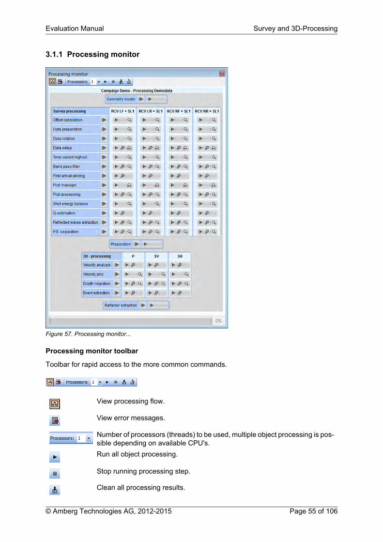
Evaluation Manual Survey and 3D-Processing
© Amberg Technologies AG, 2012-2015 Page 55 of 106
3.1.1 Processing monitor
Figure 57. Processing monitor...
Processing monitor toolbar
Toolbar for rapid access to the more common commands.
View processing flow.
View error messages.
Number of processors (threads) to be used, multiple object processing is pos-sible depending on available CPU's.Run all object processing.
Stop running processing step.
Clean all processing results.

Survey and 3D-Processing Evaluation Manual
Page 56 of 106 © Amberg Technologies AG, 2012-2015
Clean all 3D processing results.
Processing header
Header for identification of currently opened Campaign name and Processing name.
Processing objects
Column with header for identification of prepared surveys and assigned processing objects.
Run single processing step.
Open processing parameter editor for this processing step and survey.
Open seismic trace or volume viewer.
Open seismic trace viewer. Additionally, editors are available in trace view.
Run all processing steps of all surveys until here.
If there is no dongle attached, only view of processing parameters and resultsare possible.
Dongle attached, full functionality.
Red framed, parameter editor opened.
Object selected for processing.
Processing step is running.
Processing step successfully finished.
Processing step stopped due to an error.
Processing parameter editor
Computed parameter is used for processing. Inactivate the check box forparameter editing.Use default value.

Evaluation Manual Survey and 3D-Processing
© Amberg Technologies AG, 2012-2015 Page 57 of 106
Apply for all surveys. Active checkbox and inactive Computed checkbox willapply current parameter for all available survey. In combination with activeComputed check box, the computed values takes precedence over parame-ter edited by user.
3.1.2 Trace view toolbar
Figure 58. Seismic trace view toolbar
Reload content of current editor
Zoom in/out time axis
Zoom in/out offset axis
Show value function. After activation click on a trace in seismic trace view.At node position of trace, information of magnitude, time and offset is shown.
Show time range function. After activation click on a trace in seismic traceview. A time range window shows time range between beginning point andcursor position.
Open Seismic view option window
Open / close spectrum window (only if spectra are available)
Print current Seismic trace view
3.1.3 Trace view options
The Seismic trace view option is assigned to currently opened trace view windows. The optionview opens.

Survey and 3D-Processing Evaluation Manual
Page 58 of 106 © Amberg Technologies AG, 2012-2015
Trace styleVariable area shows trace in polarity col-ors (red: positive, blue: negative).
Wiggles shows seismic traces without po-larity coloring.
Show axis activates / deactivates the vi-sualisation of the trace base line.
Trace normalizationTrace normalization normalises eachtrace by its maximum amplitude. Crossnormalization normalises all traces bymaximum amplitude of entire data set. Au-tomatic gain control is a window-length-weighted normalization to let weaker sig-nals receive more gain and stronger sig-nals receiver less or none gain.Amplitude gainGain defines the gain factor of signalamplitude. The visualization of overlap-ping traces can be activated/deactivatedby Clipping.InformationAdditional trace information is shown ifavailable.Save buttonCurrent display settings will be saved andavailable for all further trace views.
Additionally, zoom in/out scale options are available for Offset and Time in the Trace view.

Evaluation Manual Survey and 3D-Processing
© Amberg Technologies AG, 2012-2015 Page 59 of 106
Offset scale zoom in/outShift + Scroll mouse wheel extends orshortens the offset axis.Time scale zoom in/outCtrl + Scroll mouse wheel extends orshortens the time axis.
3.1.4 Spectrum view
The average amplitude spectrum view displays the frequency content of the seismic traces ateach processing step. The spectra are computed for each component X,Y,Z.
Figure 59. Spectrum window
Spectrum toolbar
Zoom all.
Amplitude spectrum selection for linear or logarith-mic amplitude scaling.Selection of components to display.
As in the Trace view, the zoom in/out scale options are also available for the Spectrumwindow by using hotkeys or the mouse wheel.

Survey and 3D-Processing Evaluation Manual
Page 60 of 106 © Amberg Technologies AG, 2012-2015
3.1.5 Volume view toolbar
Figure 60. Volume view toolbar
Reload content of current editor
Open Volumetric view option window
Open / close Histogram window
Print current Volumetric view
3.1.6 Volume view options
Tab Rendering GeneralShow/hide 2D views (Longitudinal, Planand Cross section plane) together with 3Dvolume view.StationingShow distances along reference and seis-mic axis in Local distances or Tunnelme-ter.3D show volume optionsShow 3D volume in full cuboid or in threesplit planes as Longitudinal, Plan andCross section planes. Activate the surfacerendering option. Enable the 3D croppingfunctionality.
Tab Planes Plane positionsShow/hide single plane in 3D volume view.Sliders in Plane positions allow to selectLongitudinal, Plan and Cross section planeof interest in 3D volume view.

Evaluation Manual Survey and 3D-Processing
© Amberg Technologies AG, 2012-2015 Page 61 of 106
Tab Cropping Offset croppingActivate/deactivate cropping in each axe.Select minimum and maximum croppingoffset in the 3D view. It is used only whenEnable cropping in the 3D show volumeoptions of the Rendering tab is activated.
Tab Layers LayersShow/hide layers in 3D view.Shortest signal pathShow/hide Shortest signal path of waverays between shot and receiver point. Op-tion is only available in Offset calculationprocess.ButtonsSelect all and Deselect all buttons for allcheck boxes.
3.1.7 Histogram view
The Histogram is a graphical presentation of data distribution of 3D processing results. His-tograms are available for Velocity and Migration step views. The Histogram window is linkedto the volume view. The volume view appearance can be adjusted by Alpha-channel for trans-parency control and Color maps. A data minimum and maximum range can be defined to fo-cus on most relevant information. The render value used for Surface rendering option in theRendering tab can be here defined.
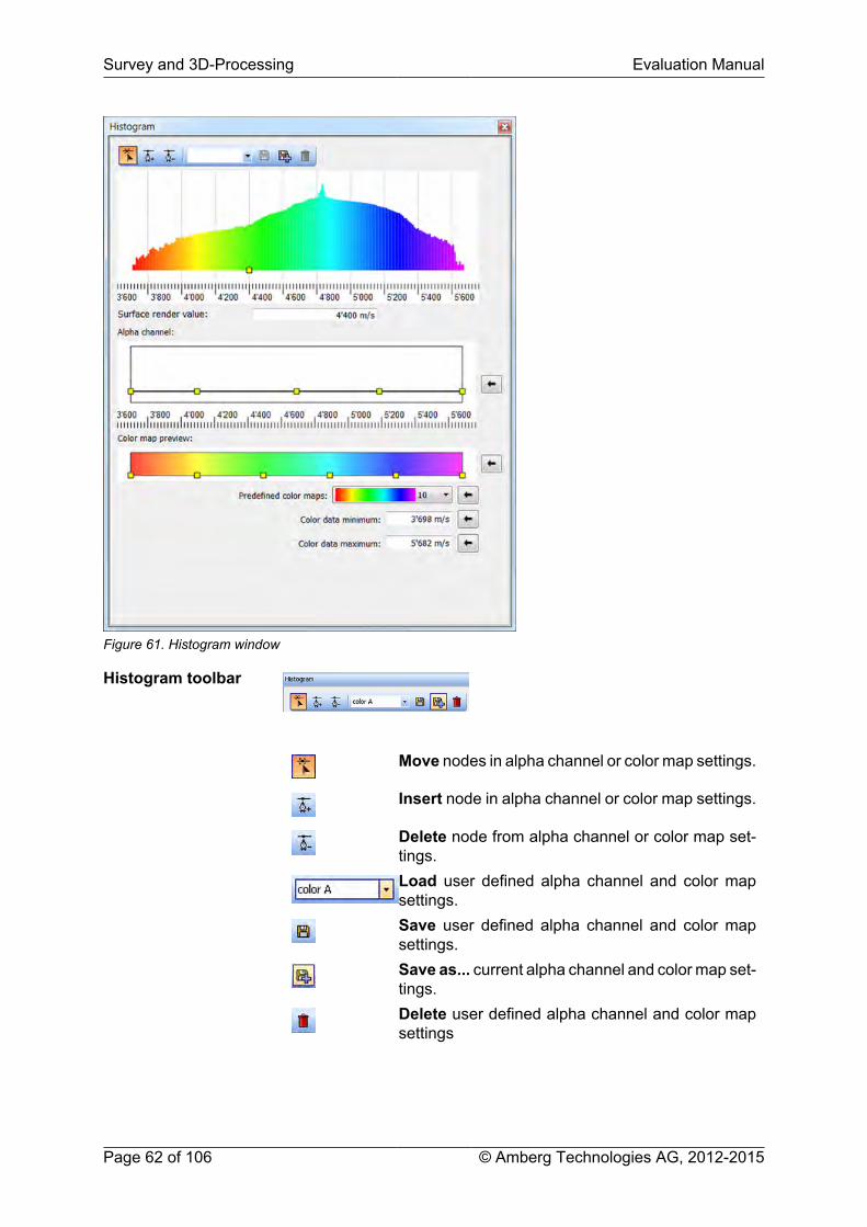
Survey and 3D-Processing Evaluation Manual
Page 62 of 106 © Amberg Technologies AG, 2012-2015
Figure 61. Histogram window
Histogram toolbar
Move nodes in alpha channel or color map settings.
Insert node in alpha channel or color map settings.
Delete node from alpha channel or color map set-tings.Load user defined alpha channel and color mapsettings.Save user defined alpha channel and color mapsettings.Save as... current alpha channel and color map set-tings.Delete user defined alpha channel and color mapsettings

Evaluation Manual Survey and 3D-Processing
© Amberg Technologies AG, 2012-2015 Page 63 of 106
Histogram settings Histogram view with automaticcolor assignment to data betweenminimum and maximum as givenin the color map settings.
Surface render value used for theSurface rendering option. The se-lected value is shown in the his-togram as a node at the bottom.Alpha channel with nodes for al-pha value settings. Arrow button:Reset Alpha channel to defaultsettings.Color map with nodes for col-or settings. Double-click on nodeopens color selection. Arrow but-ton: Reset color map to default set-tings.Load predefined color map .Click on down pointing arrowshows list of predefined colormaps. Arrow button: Load defaultcolor map.Data range settings of mini-mum and maximum value for col-or range. Buttons: Arrow button:Reset to computed minimum andmaximum value.
3.2 Step 1: Geometry Model
Description
General preparation of 3D-cuboid containing tunnel model and seismic layout. Run only pro-cess.
3.3 Step 2: Offset Calculation
Description
Calculation of survey offsets (receiver to shot line combinations) based on geometry input.Run only process. 3D visualization of ray path for each survey.
3.4 Step 3: Data Preparation
Description
Transformation of seismic raw data into TSP coordinate system. Seismic trace views avail-able.
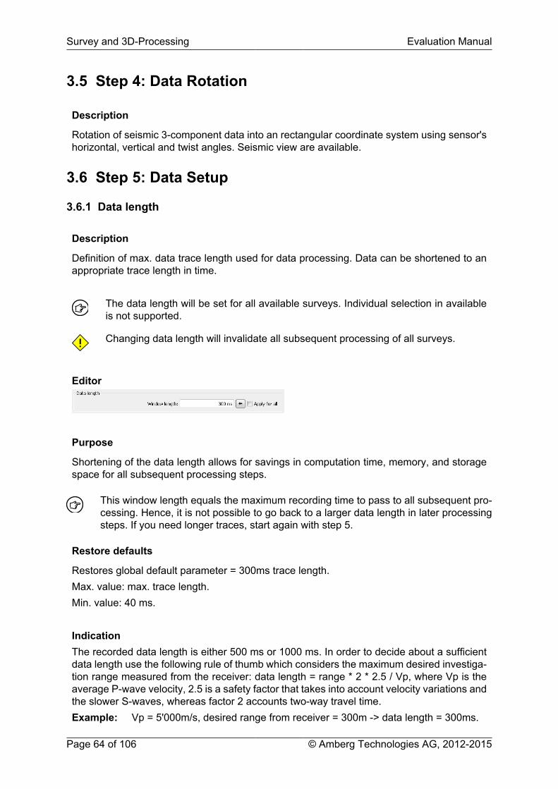
Survey and 3D-Processing Evaluation Manual
Page 64 of 106 © Amberg Technologies AG, 2012-2015
3.5 Step 4: Data Rotation
Description
Rotation of seismic 3-component data into an rectangular coordinate system using sensor'shorizontal, vertical and twist angles. Seismic view are available.
3.6 Step 5: Data Setup
3.6.1 Data length
Description
Definition of max. data trace length used for data processing. Data can be shortened to anappropriate trace length in time.
The data length will be set for all available surveys. Individual selection in availableis not supported.
Changing data length will invalidate all subsequent processing of all surveys.
Editor
Purpose
Shortening of the data length allows for savings in computation time, memory, and storagespace for all subsequent processing steps.
This window length equals the maximum recording time to pass to all subsequent pro-cessing. Hence, it is not possible to go back to a larger data length in later processingsteps. If you need longer traces, start again with step 5.
Restore defaults
Restores global default parameter = 300ms trace length.Max. value: max. trace length.Min. value: 40 ms.
IndicationThe recorded data length is either 500 ms or 1000 ms. In order to decide about a sufficientdata length use the following rule of thumb which considers the maximum desired investiga-tion range measured from the receiver: data length = range * 2 * 2.5 / Vp, where Vp is theaverage P-wave velocity, 2.5 is a safety factor that takes into account velocity variations andthe slower S-waves, whereas factor 2 accounts two-way travel time.Example: Vp = 5'000m/s, desired range from receiver = 300m -> data length = 300ms.
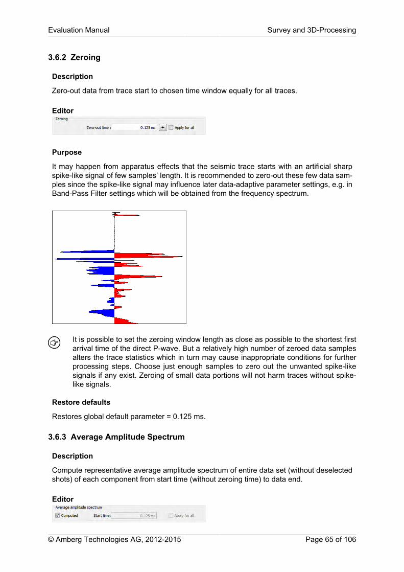
Evaluation Manual Survey and 3D-Processing
© Amberg Technologies AG, 2012-2015 Page 65 of 106
3.6.2 Zeroing
Description
Zero-out data from trace start to chosen time window equally for all traces.
Editor
Purpose
It may happen from apparatus effects that the seismic trace starts with an artificial sharpspike-like signal of few samples’ length. It is recommended to zero-out these few data sam-ples since the spike-like signal may influence later data-adaptive parameter settings, e.g. inBand-Pass Filter settings which will be obtained from the frequency spectrum.
It is possible to set the zeroing window length as close as possible to the shortest firstarrival time of the direct P-wave. But a relatively high number of zeroed data samplesalters the trace statistics which in turn may cause inappropriate conditions for furtherprocessing steps. Choose just enough samples to zero out the unwanted spike-likesignals if any exist. Zeroing of small data portions will not harm traces without spike-like signals.
Restore defaults
Restores global default parameter = 0.125 ms.
3.6.3 Average Amplitude Spectrum
Description
Compute representative average amplitude spectrum of entire data set (without deselectedshots) of each component from start time (without zeroing time) to data end.
Editor

Survey and 3D-Processing Evaluation Manual
Page 66 of 106 © Amberg Technologies AG, 2012-2015
Purpose
The average amplitude spectrum characterises the main frequency content of the seismictraces. From this spectrum, an appropriate signal frequency range is automatically extractedand taken as default for the subsequent band-pass filter parameter settings.
The spectrum display pops up automatically. If the spectrum window has been closed,open again by click on icon in toolbar.
Restore defaults
Restores global default parameter = zeroing end time
3.6.4 Spectrogram
Description
Elimination of airborne noise in time/frequency range.
Editor
Access in Data Setup view
Purpose
The occurrence of possible airborne noise may contaminate the signal and covers the realseismic information. The airborne noise signals are time dependent in the seismic tracesdue to shot to receiver offset.The time variant highcut filter takes aspect to the time dependent airborne wave using ahighcut filter combined with a time dependent frequency reduction filter curve.Non-time variant noise reduction (Min reject above = Max. reject above) : no time dependentfrequency reduction of airborne noise, only frequency highcut at equivalent Max. reject aboveand Min. reject above value.Time variant noise reduction (Min reject above < Max. reject above): maximum airbornewave reduction in time depending frequency range up to selected Max. reject above andMin. reject above value.
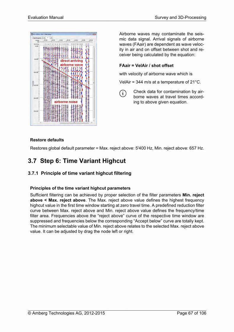
Evaluation Manual Survey and 3D-Processing
© Amberg Technologies AG, 2012-2015 Page 67 of 106
Airborne waves may contaminate the seis-mic data signal. Arrival signals of airbornewaves (FAair) are dependent as wave veloc-ity in air and on offset between shot and re-ceiver being calculated by the equation:
FAair = VelAir / shot offset
with velocity of airborne wave which is
VelAir = 344 m/s at a temperature of 21°C.
Check data for contamination by air-borne waves at travel times accord-ing to above given equation.
Restore defaults
Restores global default parameter = Max. reject above: 5'400 Hz, Min. reject above: 657 Hz.
3.7 Step 6: Time Variant Highcut
3.7.1 Principle of time variant highcut filtering
Principles of the time variant highcut parametersSufficient filtering can be achieved by proper selection of the filter parameters Min. rejectabove < Max. reject above. The Max. reject above value defines the highest frequencyhighcut value in the first time window starting at zero travel time. A predefined reduction filtercurve between Max. reject above and Min. reject above value defines the frequency/timefilter area. Frequencies above the “reject above” curve of the respective time window aresuppressed and frequencies below the corresponding “Accept below” curve are totally kept.The minimum selectable value of Min. reject above relates to the selected Max. reject abovevalue. It can be adjusted by drag the node left or right.

Survey and 3D-Processing Evaluation Manual
Page 68 of 106 © Amberg Technologies AG, 2012-2015
The maximum selectable value is Min. reject above = Max. reject above. The reduction filtercurve will then have filter characteristics equivalent to a band-pass highcut filter. This settingshould be used as bandpass prefiltering and only in case no airborne noise is contaminatingthe rawdata.
Time dependent frequency content
Noise signals may occur at later times in the frequency spectra due to airborne waves orpossible resonance effects. The noise may be significantly visible in the trace view and av-erage amplitude spectra. While the Average amplitude spectra display frequency content ofdata for all traces and within the selected time range, the spectrogram example shows the

Evaluation Manual Survey and 3D-Processing
© Amberg Technologies AG, 2012-2015 Page 69 of 106
time dependent frequency spectrum. The time variant highcut process allows to filter datawith different bandwidth at different time. The aim is to keep real seismic signals and to filtertime dependent unwanted signals.
Data setup view (rawdata)
Time variant highcut view (filtered data)
Airborne noise filter result
Depending on data, best reduction of the airborne noise can be achieved by comparison ofresult views before and after filtering.
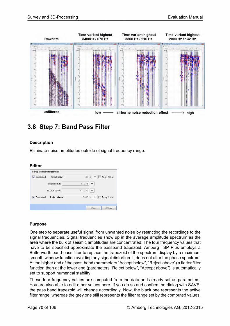
Survey and 3D-Processing Evaluation Manual
Page 70 of 106 © Amberg Technologies AG, 2012-2015
3.8 Step 7: Band Pass Filter
Description
Eliminate noise amplitudes outside of signal frequency range.
Editor
Purpose
One step to separate useful signal from unwanted noise by restricting the recordings to thesignal frequencies. Signal frequencies show up in the average amplitude spectrum as thearea where the bulk of seismic amplitudes are concentrated. The four frequency values thathave to be specified approximate the passband trapezoid. Amberg TSP Plus employs aButterworth band-pass filter to replace the trapezoid of the spectrum display by a maximumsmooth window function avoiding any signal distortion. It does not alter the phase spectrum.At the higher end of the pass-band (parameters “Accept below”, “Reject above”) a flatter filterfunction than at the lower end (parameters “Reject below”, “Accept above”) is automaticallyset to support numerical stability.These four frequency values are computed from the data and already set as parameters.You are also able to edit other values here. If you do so and confirm the dialog with SAVE,the pass band trapezoid will change accordingly. Now, the black one represents the activefilter range, whereas the grey one still represents the filter range set by the computed values.

Evaluation Manual Survey and 3D-Processing
© Amberg Technologies AG, 2012-2015 Page 71 of 106
Selected pass band frequencies have a large impact on subsequent processing andthe final result. A broader pass band increases computation time in later processing.The same filter parameters are used for all traces and components. You may check theeffectiveness of the filter by clicking on the seismic result view of following processingsteps.
Computed
Sets the frequency values reject below or reject above that have been computed from thedata and shown in the pass band trapezoid of the spectrum display.
User defined
The parameters of the Band-pass editor are directly connected to the filter results displayedin the Time variant highcut spectrum view. The Reject below and Reject above frequencyvalues can be corrected in the Bandpass editor or by drag-and-drop left or right the yellowboxes in Time variant highcut spectrum view. Inactivate the computed filter settings in Band-pass filter editor or Time variant highcut spectrum view to correct the values manually. Sav-ing the values in the Bandpass filter editor updates the filter trapezoid in the spectrum viewand vice versa.
The maximum selectable Reject above value of Bandpass filter is given by the pre-viously defined Reject above value of Time variant highcut filter.
3.9 Step 8: First Arrival Picking
Description
Determine the travel time of the direct P-wave arrival on each trace.
Editor

Survey and 3D-Processing Evaluation Manual
Page 72 of 106 © Amberg Technologies AG, 2012-2015
Purpose
Direct waves travel along the fastest path available from source to receiver. The travel timeof the direct wave is relevant to Amberg TSP Plus in order to place a short analysis windowaround the first arriving wave shape, to determine the direct wave velocity, and to supportthe shot balancing.
First arrivals (also called first breaks) are automatically detected by an algorithm thatinvestigates the trace statistics within small time windows (of specified length) that movealong the trace in order to detect significant statistical changes. It also measures thesimilarity of neighbouring traces to determine the relative shift of the bulk seismic en-ergies. An internal logic computes then the most likely location of the first break zerocrossing. If in a final quality check picks are classified to be doubtful or inconsistent thealgorithm replaces them by a travel time consistent with the general travel time trend.The automatic picks are displayed with the traces by pressing the seismic view icon ofPick Manager process.
Computed values
Sets the window length according to the frequency values which have been set in the Band-Pass Filter.
3.10 Step 9: Pick ManagerDescription
Correction of computed First arrival picks.
Trace view
Purpose
You can manually correct the computed picks (yellow boxes) by drag-and-drop up or downthe yellow box along the corresponding trace. For accurate picking use the zoom functionto enlarge the seismic scaling.
The trace views of the Pick manager open automatically depending on selected surveysand processors to be used. If only one processor is selected, only one view opens at atime. Changed and unsaved data are denoted in the view header by an asterisk (*). Afteradjustment of first arrivals the changed data need to be saved for further processing.After saving changes next survey view will open in case.
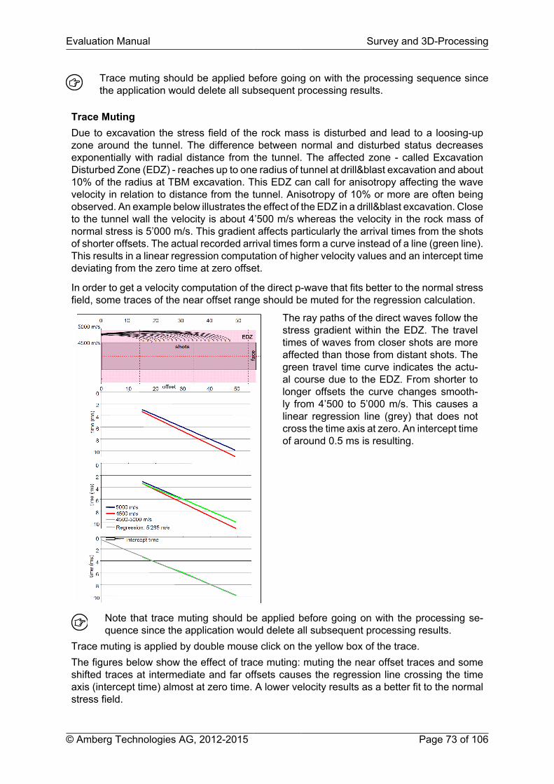
Evaluation Manual Survey and 3D-Processing
© Amberg Technologies AG, 2012-2015 Page 73 of 106
Trace muting should be applied before going on with the processing sequence sincethe application would delete all subsequent processing results.
Trace MutingDue to excavation the stress field of the rock mass is disturbed and lead to a loosing-upzone around the tunnel. The difference between normal and disturbed status decreasesexponentially with radial distance from the tunnel. The affected zone - called ExcavationDisturbed Zone (EDZ) - reaches up to one radius of tunnel at drill&blast excavation and about10% of the radius at TBM excavation. This EDZ can call for anisotropy affecting the wavevelocity in relation to distance from the tunnel. Anisotropy of 10% or more are often beingobserved. An example below illustrates the effect of the EDZ in a drill&blast excavation. Closeto the tunnel wall the velocity is about 4’500 m/s whereas the velocity in the rock mass ofnormal stress is 5’000 m/s. This gradient affects particularly the arrival times from the shotsof shorter offsets. The actual recorded arrival times form a curve instead of a line (green line).This results in a linear regression computation of higher velocity values and an intercept timedeviating from the zero time at zero offset.
In order to get a velocity computation of the direct p-wave that fits better to the normal stressfield, some traces of the near offset range should be muted for the regression calculation.
The ray paths of the direct waves follow thestress gradient within the EDZ. The traveltimes of waves from closer shots are moreaffected than those from distant shots. Thegreen travel time curve indicates the actu-al course due to the EDZ. From shorter tolonger offsets the curve changes smooth-ly from 4’500 to 5’000 m/s. This causes alinear regression line (grey) that does notcross the time axis at zero. An intercept timeof around 0.5 ms is resulting.
Note that trace muting should be applied before going on with the processing se-quence since the application would delete all subsequent processing results.
Trace muting is applied by double mouse click on the yellow box of the trace.The figures below show the effect of trace muting: muting the near offset traces and someshifted traces at intermediate and far offsets causes the regression line crossing the timeaxis (intercept time) almost at zero time. A lower velocity results as a better fit to the normalstress field.

Survey and 3D-Processing Evaluation Manual
Page 74 of 106 © Amberg Technologies AG, 2012-2015
3.11 Step 10: Pick Processing
Description
Shift whole traces in order to align first arrival picks to a line and adjustment of S-wavearrivals.
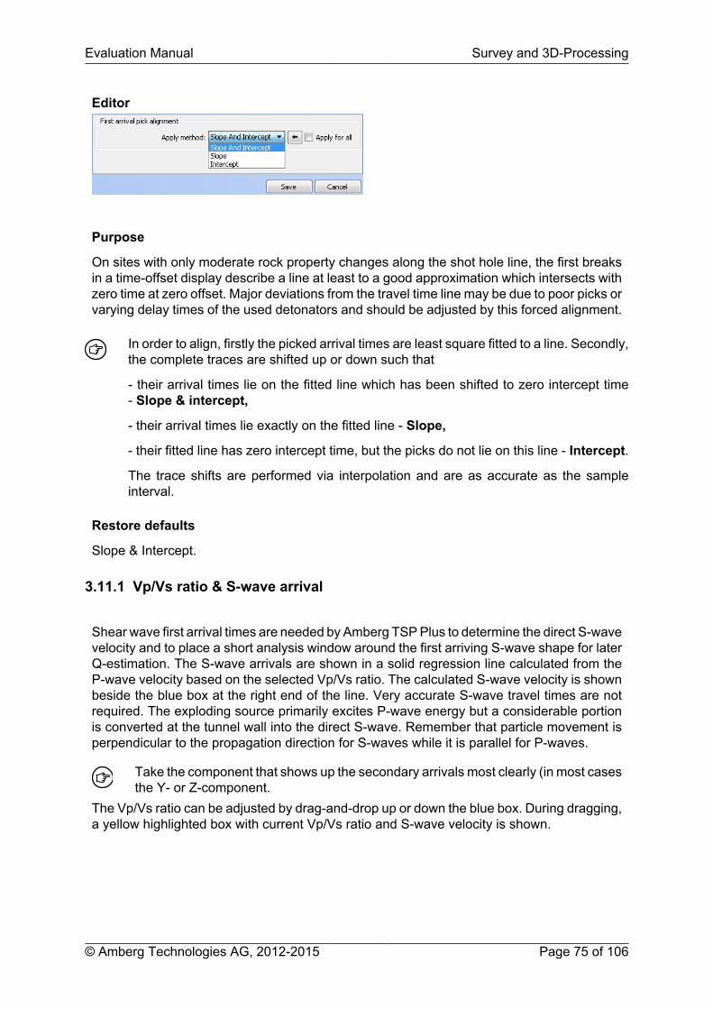
Evaluation Manual Survey and 3D-Processing
© Amberg Technologies AG, 2012-2015 Page 75 of 106
Editor
Purpose
On sites with only moderate rock property changes along the shot hole line, the first breaksin a time-offset display describe a line at least to a good approximation which intersects withzero time at zero offset. Major deviations from the travel time line may be due to poor picks orvarying delay times of the used detonators and should be adjusted by this forced alignment.
In order to align, firstly the picked arrival times are least square fitted to a line. Secondly,the complete traces are shifted up or down such that
- their arrival times lie on the fitted line which has been shifted to zero intercept time- Slope & intercept,
- their arrival times lie exactly on the fitted line - Slope,
- their fitted line has zero intercept time, but the picks do not lie on this line - Intercept.
The trace shifts are performed via interpolation and are as accurate as the sampleinterval.
Restore defaults
Slope & Intercept.
3.11.1 Vp/Vs ratio & S-wave arrival
Shear wave first arrival times are needed by Amberg TSP Plus to determine the direct S-wavevelocity and to place a short analysis window around the first arriving S-wave shape for laterQ-estimation. The S-wave arrivals are shown in a solid regression line calculated from theP-wave velocity based on the selected Vp/Vs ratio. The calculated S-wave velocity is shownbeside the blue box at the right end of the line. Very accurate S-wave travel times are notrequired. The exploding source primarily excites P-wave energy but a considerable portionis converted at the tunnel wall into the direct S-wave. Remember that particle movement isperpendicular to the propagation direction for S-waves while it is parallel for P-waves.
Take the component that shows up the secondary arrivals most clearly (in most casesthe Y- or Z-component.
The Vp/Vs ratio can be adjusted by drag-and-drop up or down the blue box. During dragging,a yellow highlighted box with current Vp/Vs ratio and S-wave velocity is shown.
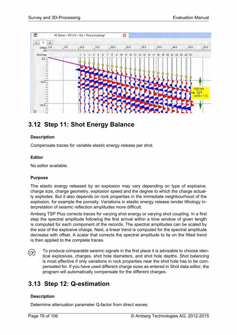
Survey and 3D-Processing Evaluation Manual
Page 76 of 106 © Amberg Technologies AG, 2012-2015
3.12 Step 11: Shot Energy Balance
Description
Compensate traces for variable elastic energy release per shot.
Editor
No editor available.
Purpose
The elastic energy released by an explosion may vary depending on type of explosive,charge size, charge geometry, explosion speed and the degree to which the charge actual-ly explodes. But it also depends on rock properties in the immediate neighbourhood of theexplosion, for example the porosity. Variations in elastic energy release render lithology in-terpretation of seismic reflection amplitudes more difficult.Amberg TSP Plus corrects traces for varying shot energy or varying shot coupling. In a firststep the spectral amplitude following the first arrival within a time window of given lengthis computed for each component of the records. The spectral amplitudes can be scaled bythe size of the explosive charge. Next, a linear trend is computed for the spectral amplitudedecrease with offset. A scalar that corrects the spectral amplitude to lie on the fitted trendis then applied to the complete traces.
To produce comparable seismic signals in the first place it is advisable to choose iden-tical explosives, charges, shot hole diameters, and shot hole depths. Shot balancingis most effective if only variations in rock properties near the shot hole has to be com-pensated for. If you have used different charge sizes as entered in Shot data editor, theprogram will automatically compensate for the different charges.
3.13 Step 12: Q-estimation
Description
Determine attenuation parameter Q-factor from direct waves.

Evaluation Manual Survey and 3D-Processing
© Amberg Technologies AG, 2012-2015 Page 77 of 106
Editor
Purpose
While propagating through rock, seismic P-waves and S-waves lose in strength mainly bythree processes: (1) As the wavefront expands, the source energy is distributed on an ex-panding area and the amplitude per unit area decreases linearly with distance and time in ahomogeneous rock. This is the geometrical spreading loss. (2) When rock heterogeneitiesare encountered, portions of the wave energy change propagation direction slightly or theyare reflected. Heterogeneities that are larger than about a tenth of the dominating wavelengthcause reflection loss. Inhomogeneities with dimensions clearly below the seismic wavelengthresult in scattering attenuation. (3) Intrinsic attenuation, also called absorption, converts waveenergy into heat.
For the whole receiver gather a Q-factor from the direct P-wave and of each componentis estimated. From these three values the maximum is selected and shown as Q-factorin the editor of the subsequent step of the corresponding survey. Ideally, the windowaround the first break used for Q-estimation should only contain the primary pulse andthis pulse must not be truncated. If in doubt select the Amberg TSP Plus default.
Computed values
Sets the window length according to the primary pulse values.
3.14 Step 13: Reflected waves extraction
Description
Dip filtering to extract reflected waves and partially reverse wave attenuation.
Editor
Purpose Radon transformAmong the various wave types recorded by the TSP 303 receivers only waves that have beenreflected ahead of the tunnel face and from beside the tunnel carry information about rockheterogeneities ahead and only they should later be imaged. Those reflected waves can beseparated from other wave modes by a dip filter in the offset-time section because in the TSPacquisition geometry, reflected waves from ahead reach the receiver the later the larger thedistance of the shot from the tunnel face. Direct waves have dips with reverse sign because

Survey and 3D-Processing Evaluation Manual
Page 78 of 106 © Amberg Technologies AG, 2012-2015
they reach the receiver the earlier the smaller the source-receiver offset. Amberg TSP Plusextracts reflected wave dips via an algorithm that transforms the time–space section intofrequency-dip space, zeros unwanted dips, and performs a backward transformation of theremaining dips to the time-space domain. A transformation into dip-space is called a linearRadon transform.
Temporarily Amberg TSP Plus can interpolate extra traces to relax the strict aliasinglimit for the Radon transform. The user may reduce the Min. Move out value, for exampleto focus on reflections that dip only slightly towards the tunnel axis.
Computed values
Sets the Min. Move out according to the frequency values that have been set in the Band-Pass Filter.
Purpose Inverse Q-filtering
Energy loss due to attenuation weakens particularly the high frequencies within the signalpassband. This restricts the seismic resolution, especially at large distances. The estimatedquality factor Q of the rock can partially restore the lost amplitudes by an inverse Q-filter-ing. Amplitudes cannot be restored if the signal has been weakened below the backgroundnoise level. An upper amplitude gain limit (i.e. max Gain= 25 dB) avoids that the backgroundnoise is blown up. Amberg TSP Plus performs the amplitude restoration in the frequencydomain, where the gain function is smoothly tapered down beyond the gain limit for numer-ical reasons. For physical reasons attenuation not only reduces amplitudes but also yieldsdispersion, i.e. frequency dependent propagation velocities. A seismic pulse that enters anattenuating medium broadens during propagation not only due to boosted amplitude loss athigh frequencies but also because its high signal frequency components travel faster thanits low frequency components. That changes the phase relations between frequencies withtime. The estimated Q-factor allows to completely reverse the Q-related pulse dispersion.
Usually amplitude loss and phase distortion should be compensated. Phase compen-sation works on the fly. Even after inverse amplitude compensation seismic amplitudesmay decrease with distance due to the gain limit but also because of reflection loss thatis not accounted for.
Computed values
Sets upper amplitude gain limit (Max. gain) computed by signal/noise ratio.
Q-factors characterise the micro structure of rock and may vary by about two ordersof magnitude from 10 to 500. But typical TSP data reveals Q-factors in the range of20-50. Small Q-factors indicate large attenuation and heterogeneous micro structure.Q-factors vary from rock to rock but also for given rock types dependent on the specificconditions at a particular tunnelling site. The variations from site to site for a particularrock type may often be larger than the variations from rock type to rock type. Neverthe-less, some general rules concerning Q can be formulated: The presence of fractures,micro cracks and other defects in the solid rock material yield an increase of attenua-tion (lower Q-factors). Attenuation decreases with increasing earth pressure, where thepressure dependence is strongest at low pressures, i.e. close to the surface. The atten-uation in brine- or water saturated rocks is higher than for dry or gas saturated rocks.In dry and gas saturated rocks Qp is slightly lower than Qs, in water saturated rock Qpis distinctly higher than Qs (shear waves do not propagate in fluids). Attenuation tendsto increase with porosity.

Evaluation Manual Survey and 3D-Processing
© Amberg Technologies AG, 2012-2015 Page 79 of 106
Computed values
Sets the estimated Q-factor.
3.15 Step 14: P.S. Separation
Description
Transforms the X-, Y- and Z-component records into P-, SH- and SV-wave components.
Editor
Purpose
Compressional waves (P-waves) and shear waves (S-waves) are characterised by specif-ic particle movements. The longitudinal P-waves force rock particles to move forward andbackward in the propagation direction. S-waves are transversal waves, i.e. particle motion isperpendicular to propagation direction. Shear waves cause an ellipsoidal particle movementwhere the movement along the ellipsoid is retrograde, i.e. counter-clockwise. SV-waves arepolarised such that the motion is in the vertical plane that also contains the direction of wavepropagation. SH-waves are polarised so that the motion is in the horizontal plane that alsocontains the direction of wave propagation. In general, S-waves have SV- and SH-compo-nents. With three component registrations, P-waves, SH-waves and SV-waves can be ob-tained from the X-, Y- and Z-components. Amberg TSP Plus separates the recordings intowave types via rotating the coordinate system as function of recording time.
It is recommended to use the default time window length for rotation angle estimation.If the window is too small the angle may fluctuate strongly from sample to sample dueto random noise components, if it is too large subsequently arriving waves may havetheir incidence angles mixed up. Note that only one wave mode (and incidence angle)may be computed at a given time. If two waves arrive at the same time from differentdirections the stronger event may dominate the rotation angle computation and theweaker event will be suppressed.
Computed values
Sets the Time window according to the primary pulse value.
3.16 Step 15: Preparation
Description
Concatenation of wave types of available surveys and preparation for 3D-processing. Noview available.
Editor
No editor available.
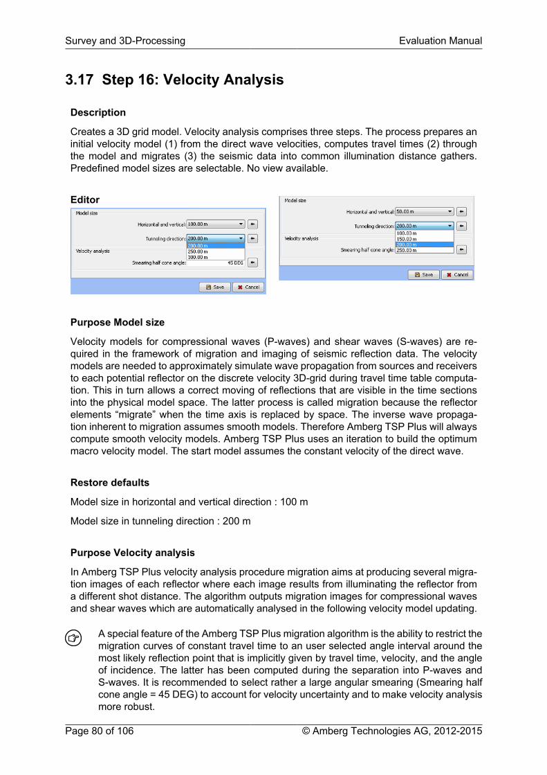
Survey and 3D-Processing Evaluation Manual
Page 80 of 106 © Amberg Technologies AG, 2012-2015
3.17 Step 16: Velocity Analysis
Description
Creates a 3D grid model. Velocity analysis comprises three steps. The process prepares aninitial velocity model (1) from the direct wave velocities, computes travel times (2) throughthe model and migrates (3) the seismic data into common illumination distance gathers.Predefined model sizes are selectable. No view available.
Editor
Purpose Model size
Velocity models for compressional waves (P-waves) and shear waves (S-waves) are re-quired in the framework of migration and imaging of seismic reflection data. The velocitymodels are needed to approximately simulate wave propagation from sources and receiversto each potential reflector on the discrete velocity 3D-grid during travel time table computa-tion. This in turn allows a correct moving of reflections that are visible in the time sectionsinto the physical model space. The latter process is called migration because the reflectorelements “migrate” when the time axis is replaced by space. The inverse wave propaga-tion inherent to migration assumes smooth models. Therefore Amberg TSP Plus will alwayscompute smooth velocity models. Amberg TSP Plus uses an iteration to build the optimummacro velocity model. The start model assumes the constant velocity of the direct wave.
Restore defaults
Model size in horizontal and vertical direction : 100 m
Model size in tunneling direction : 200 m
Purpose Velocity analysis
In Amberg TSP Plus velocity analysis procedure migration aims at producing several migra-tion images of each reflector where each image results from illuminating the reflector froma different shot distance. The algorithm outputs migration images for compressional wavesand shear waves which are automatically analysed in the following velocity model updating.
A special feature of the Amberg TSP Plus migration algorithm is the ability to restrict themigration curves of constant travel time to an user selected angle interval around themost likely reflection point that is implicitly given by travel time, velocity, and the angleof incidence. The latter has been computed during the separation into P-waves andS-waves. It is recommended to select rather a large angular smearing (Smearing halfcone angle = 45 DEG) to account for velocity uncertainty and to make velocity analysismore robust.
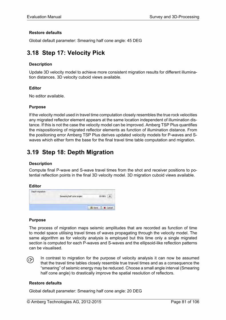
Evaluation Manual Survey and 3D-Processing
© Amberg Technologies AG, 2012-2015 Page 81 of 106
Restore defaults
Global default parameter: Smearing half cone angle: 45 DEG
3.18 Step 17: Velocity Pick
Description
Update 3D velocity model to achieve more consistent migration results for different illumina-tion distances. 3D velocity cuboid views available.
Editor
No editor available.
Purpose
If the velocity model used in travel time computation closely resembles the true rock velocitiesany migrated reflector element appears at the same location independent of illumination dis-tance. If this is not the case the velocity model can be improved. Amberg TSP Plus quantifiesthe mispositioning of migrated reflector elements as function of illumination distance. Fromthe positioning error Amberg TSP Plus derives updated velocity models for P-waves and S-waves which either form the base for the final travel time table computation and migration.
3.19 Step 18: Depth Migration
DescriptionCompute final P-wave and S-wave travel times from the shot and receiver positions to po-tential reflection points in the final 3D velocity model. 3D migration cuboid views available.
Editor
Purpose
The process of migration maps seismic amplitudes that are recorded as function of timeto model space utilising travel times of waves propagating through the velocity model. Thesame algorithm as for velocity analysis is employed but this time only a single migratedsection is computed for each P-waves and S-waves and the ellipsoid-like reflection patternscan be visualised.
In contrast to migration for the purpose of velocity analysis it can now be assumedthat the travel time tables closely resemble true travel times and as a consequence the“smearing” of seismic energy may be reduced. Choose a small angle interval (Smearinghalf cone angle) to drastically improve the spatial resolution of reflectors.
Restore defaults
Global default parameter: Smearing half cone angle: 20 DEG

Survey and 3D-Processing Evaluation Manual
Page 82 of 106 © Amberg Technologies AG, 2012-2015
3.20 Step 19: Event extractionDescription
Extract dominant P-wave and S-wave reflectors from the final migration result using imageprocessing and segmentation. No views available.
Editor
Purpose
The final migration result may show many ellipsoid-like bodies with image amplitudes varyingalong each of the bodies and also between them. For tunnelling, only the most prominentreflection elements are of interest. Therefore, Amberg TSP Plus extracts a user-suppliednumber of most significant P-wave and S-wave reflectors. The algorithm works in two steps:
1. It balances the migrated section to remove general trends in reflection amplitudes (like ageneral decrease with distance due to incomplete inverse Q amplitude compensation).
2. It simplifies the image by omitting insignificant events and groups reflection points to re-flector segments.
Section balancing and segmentation run in iteration. If many reflector elements are re-quested computation time increases. When N Reflectors are requested the N most sig-nificant reflectors are written out. If there are not N reflectors on all the components, theresulting number of reflectors may be less than N. To specify more than about 20 reflec-tor elements may render interpretation too complex. To guide the image segmentationthe upper Coverage quantile % to select reflection coverage for the extraction processcan be specified. If the value is set to 20 percent than this means that coverage mustbe among the upper 20 percent traces have to contribute to the migrated amplitude inthe section (after balancing) in order to be considered for reflector extraction.
Restore defaults
Coverage quantile: 20 %Number of reflectors: 5
3.21 Step 20: Reflector extractionDescription
Concatenation of all extracted elements and positioning with 3D-cuboids. Preparation of ex-tracted reflectors from the migration result and segmentation for Evaluation set.
Editor
No editor available.

Evaluation Manual Survey and 3D-Processing
© Amberg Technologies AG, 2012-2015 Page 83 of 106
Purpose
The event extraction is being applied individually for each wave component (P, SH, SV). Inthis step the program examines all extracted reflector segments in each component to findcorresponding reflector segments at same locations among all wave components. At the endextracted reflector segments are located at or near same locations between the components.Now, reflectors become comparable and are being filtered according to their magnitude.
It computes for each segment parameters like size, spatial orientation or intersection pointwith the tunnel axis. Finally, geometric and rock mechanical parameters each remainingsegments is being computed and forwarded to the evaluation set.

Page 84 of 106

Evaluation Manual
© Amberg Technologies AG, 2012-2015 Page 85 of 106
Chapter 4 Result Evaluation4.1 Evaluation setOnce at least one survey has been completely processed the Evaluation set can be opened.Open the Evaluation set editor by double-click on the corresponding node in the project tree.An editor opens with access to following view:
Figure 62. Evaluation set editor
Charts (1) Rock property charts of parameters selected via the Options tab.2D/3D views (2) 2D and 3D visualisation of selected parameter. In the 2D tab,
longitudinal or plan view can be selected. In the 3D tab, a 3Dperspective view presents the tunnel environment and reflectorswith color shading in between them based on a selected rockproperty. When using the 2D tab, panes (1) and (2) are linkedwith each other in a way that zooming and panning work similarlyand option settings are being shared.
Evaluation table (3) List of extracted reflector segments including rock mechanicaland physical parameters and interpretation tools option.
View options (4) Option window for Charts reflector table and 2D and 3D settings.
Once an Evaluation set has been generated after the last 3D-Processing step has beensuccessfully finished, it remains as long as new 3D-processing is finished next time.
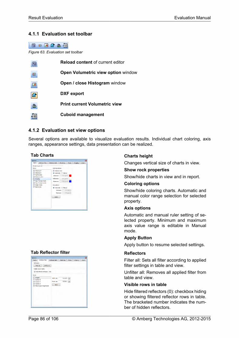
Result Evaluation Evaluation Manual
Page 86 of 106 © Amberg Technologies AG, 2012-2015
4.1.1 Evaluation set toolbar
Figure 63. Evaluation set toolbar
Reload content of current editor
Open Volumetric view option window
Open / close Histogram window
DXF export
Print current Volumetric view
Cuboid management
4.1.2 Evaluation set view options
Several options are available to visualize evaluation results. Individual chart coloring, axisranges, appearance settings, data presentation can be realized.
Tab Charts Charts heightChanges vertical size of charts in view.Show rock propertiesShow/hide charts in view and in report.Coloring optionsShow/hide coloring charts. Automatic andmanual color range selection for selectedproperty.Axis optionsAutomatic and manual ruler setting of se-lected property. Minimum and maximumaxis value range is editable in Manualmode.Apply ButtonApply button to resume selected settings.
Tab Reflector filter ReflectorsFilter all: Sets all filter according to appliedfilter settings in table and view.Unfilter all: Removes all applied filter fromtable and view.Visible rows in tableHide filtered reflectors (0): checkbox hidingor showing filtered reflector rows in table.The bracketed number indicates the num-ber of hidden reflectors.

Evaluation Manual Result Evaluation
© Amberg Technologies AG, 2012-2015 Page 87 of 106
Apply:Length: Min. to max. length of reflectors;defaults are the values from the extractedreflectors (= no filter).Center X: Min. to max. center points alongthe tunnel axis (X); defaults are the valuesfrom the extracted reflectors (= no filter).Center Y: Min. to max. center points of lat-eral model extension (Y); defaults are thevalues from the extracted reflectors (= nofilter).Center Z: Min. to max. center points of ver-tical model extension (Z); defaults are thevalues from the extracted reflectors (= nofilter).Wave type magnitude: magnitude filter ofextracted reflector triple (P/SV/SH).- all: show entire reflector triple- largest: show only reflector with largestmagnitude of triple- largest & 2. largest show reflectors withlargest & 2. largest magnitude of triple
Tab Reflector table ReflectorsMute all and Unmute all buttons.Visible rows in tableShow/hide muted reflectors in table and re-port.Visible columns in tableShow/hide visible columns in table and inreport.
Only selected columns are listed inreport table for printing.
It is recommended to reduce se-lected columns to the number ofproperties to be presented.
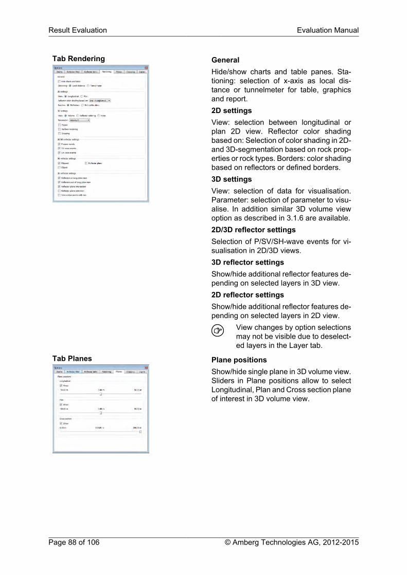
Result Evaluation Evaluation Manual
Page 88 of 106 © Amberg Technologies AG, 2012-2015
Tab Rendering GeneralHide/show charts and table panes. Sta-tioning: selection of x-axis as local dis-tance or tunnelmeter for table, graphicsand report.2D settingsView: selection between longitudinal orplan 2D view. Reflector color shadingbased on: Selection of color shading in 2D-and 3D-segmentation based on rock prop-erties or rock types. Borders: color shadingbased on reflectors or defined borders.3D settingsView: selection of data for visualisation.Parameter: selection of parameter to visu-alise. In addition similar 3D volume viewoption as described in 3.1.6 are available.2D/3D reflector settingsSelection of P/SV/SH-wave events for vi-sualisation in 2D/3D views.3D reflector settingsShow/hide additional reflector features de-pending on selected layers in 3D view.2D reflector settingsShow/hide additional reflector features de-pending on selected layers in 2D view.
View changes by option selectionsmay not be visible due to deselect-ed layers in the Layer tab.
Tab Planes Plane positionsShow/hide single plane in 3D volume view.Sliders in Plane positions allow to selectLongitudinal, Plan and Cross section planeof interest in 3D volume view.

Evaluation Manual Result Evaluation
© Amberg Technologies AG, 2012-2015 Page 89 of 106
Tab Cropping Offset CroppingActivate/deactivate cropping in each axe.Select minimum and maximum croppingoffset in the 3D view. It is used only whenEnable cropping in the 3D show volumeoptions of the Rendering tab is activated.
Tab Layers LayersShow/hide layers in 2D and 3D view.ButtonsOption on select / deselect all layers fordisplay.
4.1.3 Charts view
The charts view displays rock physical and mechanical parameters as selected via the tabCharts in the Options window. The charts correspond to the parameter values along the seismicaxis for 2D longitudinal view (Y=0) or 2D plan view (Z=0). The length and color shading of eachsegment is initially defined according to the extracted reflectors. This can be later modified byusing the option mute reflector or reflector filtering.
For each selected parameter an initial Reference value is indicated. This value correspondsto the value behind the first reflector segment within the TSP layout derived from the directwave velocities. The Reference value represents a middle node of a color palette editable inthe Manual mode of the Coloring options. The color palette is generated by selecting colors forthe maximum, minimum and reference value.
Figure 64. Chart pane displaying selected rock mechanical parameters…
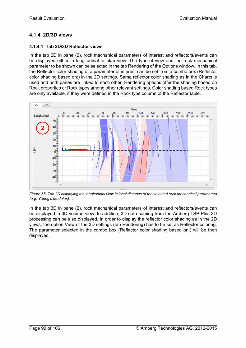
Result Evaluation Evaluation Manual
Page 90 of 106 © Amberg Technologies AG, 2012-2015
4.1.4 2D/3D views
4.1.4.1 Tab 2D/3D Reflector views
In the tab 2D in pane (2), rock mechanical parameters of interest and reflectors/events canbe displayed either in longitudinal or plan view. The type of view and the rock mechanicalparameter to be shown can be selected in the tab Rendering of the Options window. In this tab,the Reflector color shading of a parameter of interest can be set from a combo box (Reflectorcolor shading based on:) in the 2D settings. Same reflector color shading as in the Charts isused and both panes are linked to each other. Rendering options offer the shading based onRock properties or Rock types among other relevant settings. Color shading based Rock typesare only available, if they were defined in the Rock type column of the Reflector table.
Figure 65. Tab 2D displaying the longitudinal view in local distance of the selected rock mechanical parameters(e.g. Young's Modulus)…
In the tab 3D in pane (2), rock mechanical parameters of interest and reflectors/events canbe displayed in 3D volume view. In addition, 3D data coming from the Amberg TSP Plus 3Dprocessing can be also displayed. In order to display the reflector color shading as in the 2Dviews, the option View of the 3D settings (tab Rendering) has to be set as Reflector coloring.The parameter selected in the combo box (Reflector color shading based on:) will be thendisplayed.

Evaluation Manual Result Evaluation
© Amberg Technologies AG, 2012-2015 Page 91 of 106
Figure 66. Tab 3D displaying the volume view in local distance of the selected rock mechanical parameters(e.g. Young's Modulus)…
Reflector color shading in 2D and 3D view
User can decide, whether color shading of selected rock mechanical parameter is based onreflector borders or on defined borders with geological segmentation. In the following, reflec-tors crossing the 2D longitudinal or plan plane are colored red/blue «in the longitudinal/planview» according to their reflectivity. Reflectors not crossing the 2D longitudinal or plan view(«out of the longitudinal/plan view») are colored dark grey. This nomenclature is also valid forreflector planes, ellipsoids in 3D views. The interpolation of the reflectors extensions on thelongitudinal/plan view is shown as red/blue colored «reflector plane intersection or extensions».Reflector elements as borders are black colored and bolt.
Reflector color shading based on select-ed rock mechanical parameter
Segmentation is color shaded betweeneach reflector element based on the se-lected rock mechanical parameter value.
Defined border color shading based onselected rock mechanical parameter
Segmentation is color shaded betweeneach defined border element based on theselected rock mechanical parameter val-ue.
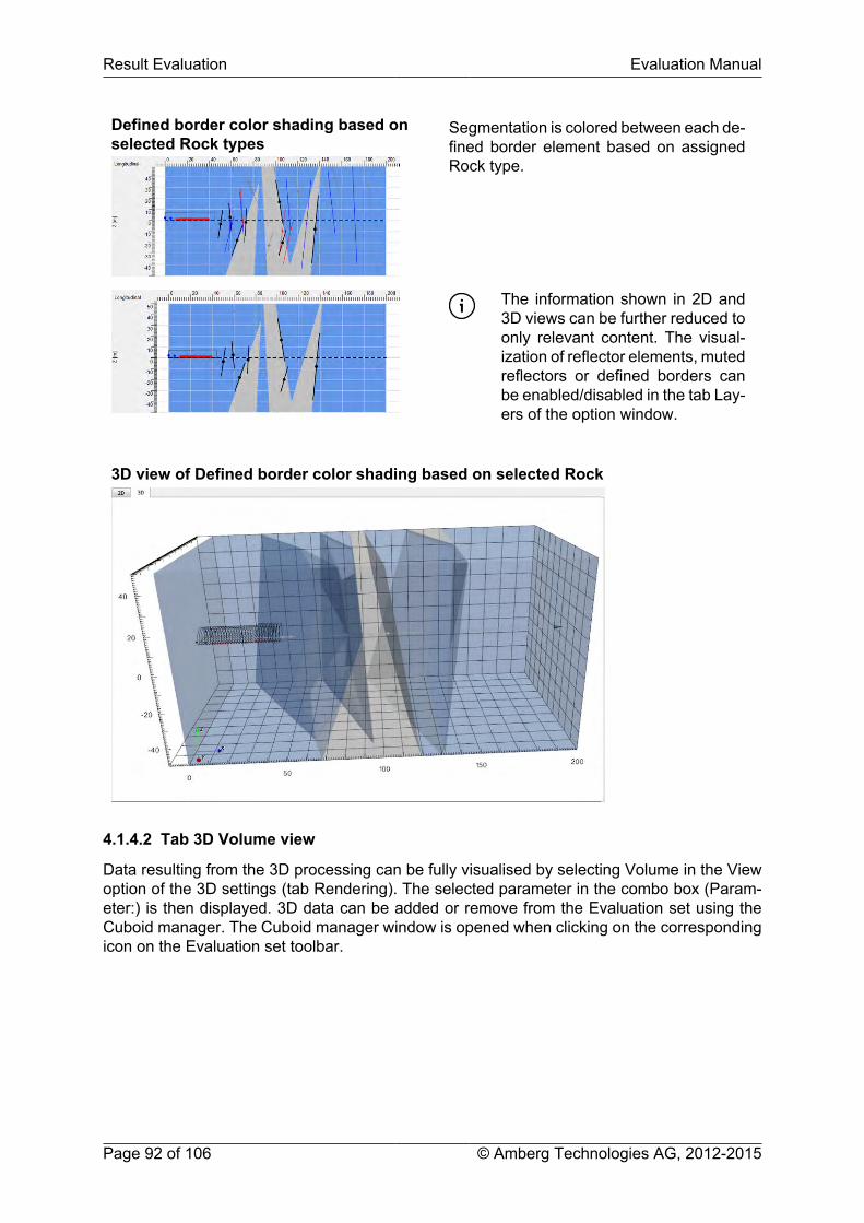
Result Evaluation Evaluation Manual
Page 92 of 106 © Amberg Technologies AG, 2012-2015
Defined border color shading based onselected Rock types
Segmentation is colored between each de-fined border element based on assignedRock type.
The information shown in 2D and3D views can be further reduced toonly relevant content. The visual-ization of reflector elements, mutedreflectors or defined borders canbe enabled/disabled in the tab Lay-ers of the option window.
3D view of Defined border color shading based on selected Rock
4.1.4.2 Tab 3D Volume view
Data resulting from the 3D processing can be fully visualised by selecting Volume in the Viewoption of the 3D settings (tab Rendering). The selected parameter in the combo box (Param-eter:) is then displayed. 3D data can be added or remove from the Evaluation set using theCuboid manager. The Cuboid manager window is opened when clicking on the correspondingicon on the Evaluation set toolbar.
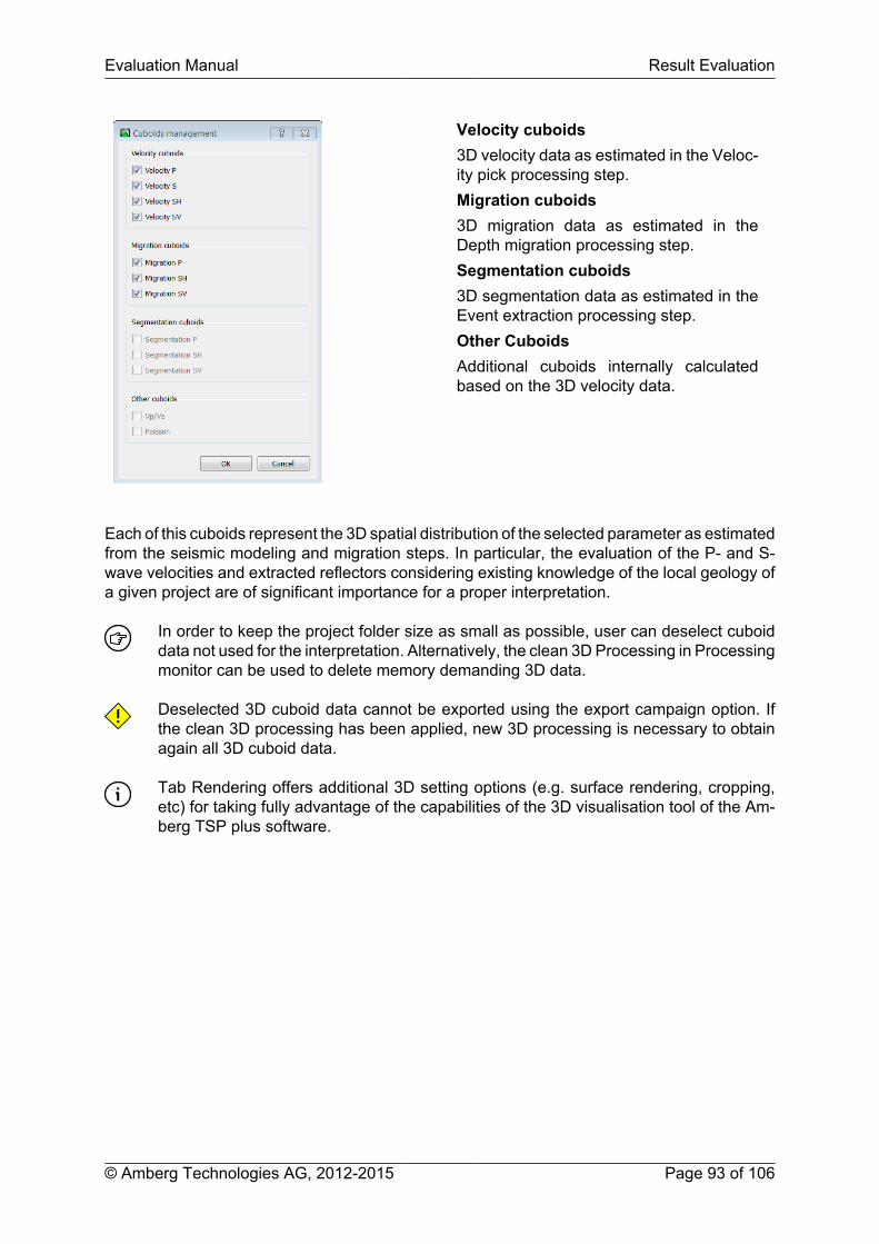
Evaluation Manual Result Evaluation
© Amberg Technologies AG, 2012-2015 Page 93 of 106
Velocity cuboids3D velocity data as estimated in the Veloc-ity pick processing step.Migration cuboids3D migration data as estimated in theDepth migration processing step.Segmentation cuboids3D segmentation data as estimated in theEvent extraction processing step.Other CuboidsAdditional cuboids internally calculatedbased on the 3D velocity data.
Each of this cuboids represent the 3D spatial distribution of the selected parameter as estimatedfrom the seismic modeling and migration steps. In particular, the evaluation of the P- and S-wave velocities and extracted reflectors considering existing knowledge of the local geology ofa given project are of significant importance for a proper interpretation.
In order to keep the project folder size as small as possible, user can deselect cuboiddata not used for the interpretation. Alternatively, the clean 3D Processing in Processingmonitor can be used to delete memory demanding 3D data.
Deselected 3D cuboid data cannot be exported using the export campaign option. Ifthe clean 3D processing has been applied, new 3D processing is necessary to obtainagain all 3D cuboid data.
Tab Rendering offers additional 3D setting options (e.g. surface rendering, cropping,etc) for taking fully advantage of the capabilities of the 3D visualisation tool of the Am-berg TSP plus software.
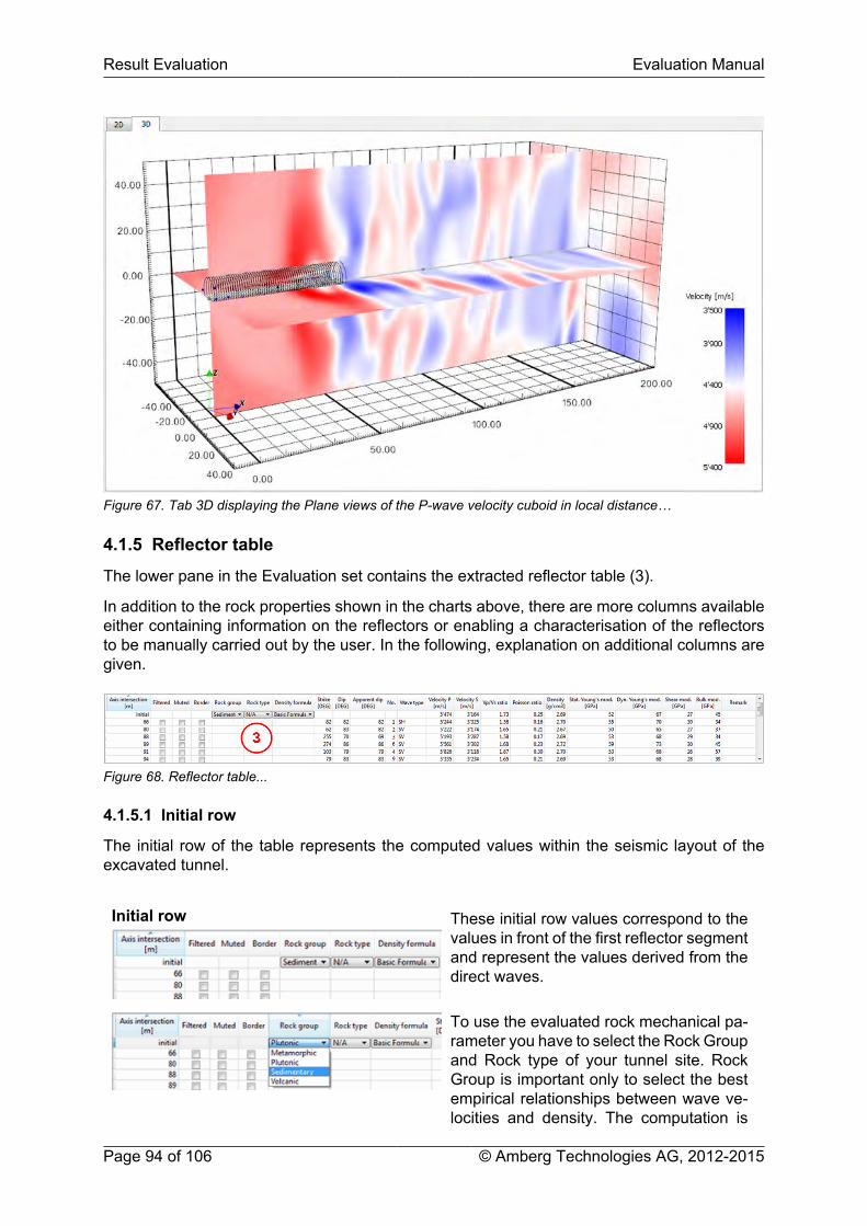
Result Evaluation Evaluation Manual
Page 94 of 106 © Amberg Technologies AG, 2012-2015
Figure 67. Tab 3D displaying the Plane views of the P-wave velocity cuboid in local distance…
4.1.5 Reflector table
The lower pane in the Evaluation set contains the extracted reflector table (3).
In addition to the rock properties shown in the charts above, there are more columns availableeither containing information on the reflectors or enabling a characterisation of the reflectorsto be manually carried out by the user. In the following, explanation on additional columns aregiven.
Figure 68. Reflector table...
4.1.5.1 Initial row
The initial row of the table represents the computed values within the seismic layout of theexcavated tunnel.
Initial row These initial row values correspond to thevalues in front of the first reflector segmentand represent the values derived from thedirect waves.
To use the evaluated rock mechanical pa-rameter you have to select the Rock Groupand Rock type of your tunnel site. RockGroup is important only to select the bestempirical relationships between wave ve-locities and density. The computation is
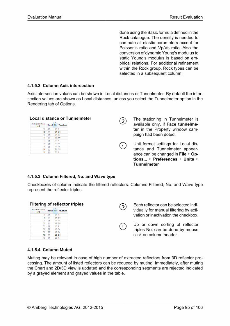
Evaluation Manual Result Evaluation
© Amberg Technologies AG, 2012-2015 Page 95 of 106
done using the Basic formula defined in theRock catalogue. The density is needed tocompute all elastic parameters except forPoisson's ratio and Vp/Vs ratio. Also theconversion of dynamic Young's modulus tostatic Young's modulus is based on em-pirical relations. For additional refinementwithin the Rock group, Rock types can beselected in a subsequent column.
4.1.5.2 Column Axis intersection
Axis intersection values can be shown in Local distances or Tunnelmeter. By default the inter-section values are shown as Local distances, unless you select the Tunnelmeter option in theRendering tab of Options.
Local distance or Tunnelmeter The stationing in Tunnelmeter isavailable only, if Face tunnelme-ter in the Property window cam-paign had been doted.
Unit format settings for Local dis-tance and Tunnelmeter appear-ance can be changed in File ▶ Op-tions... ▶ Preferences ▶ Units ▶Tunnelmeter
4.1.5.3 Column Filtered, No. and Wave type
Checkboxes of column indicate the filtered reflectors. Columns Filtered, No. and Wave typerepresent the reflector triples.
Filtering of reflector triples Each reflector can be selected indi-vidually for manual filtering by acti-vation or inactivation the checkbox.
Up or down sorting of reflectortriples No. can be done by mouseclick on column header.
4.1.5.4 Column Muted
Muting may be relevant in case of high number of extracted reflectors from 3D reflector pro-cessing. The amount of listed reflectors can be reduced by muting. Immediately, after mutingthe Chart and 2D/3D view is updated and the corresponding segments are rejected indicatedby a grayed element and grayed values in the table.
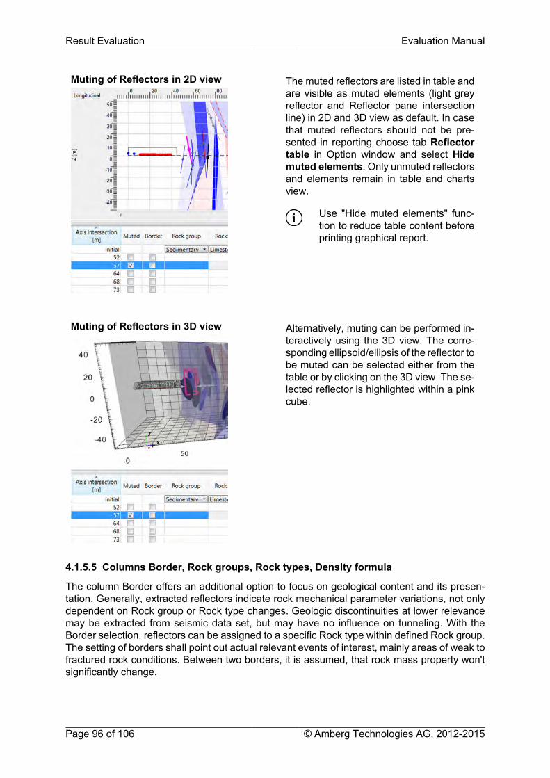
Result Evaluation Evaluation Manual
Page 96 of 106 © Amberg Technologies AG, 2012-2015
Muting of Reflectors in 2D view The muted reflectors are listed in table andare visible as muted elements (light greyreflector and Reflector pane intersectionline) in 2D and 3D view as default. In casethat muted reflectors should not be pre-sented in reporting choose tab Reflectortable in Option window and select Hidemuted elements. Only unmuted reflectorsand elements remain in table and chartsview.
Use "Hide muted elements" func-tion to reduce table content beforeprinting graphical report.
Muting of Reflectors in 3D view Alternatively, muting can be performed in-teractively using the 3D view. The corre-sponding ellipsoid/ellipsis of the reflector tobe muted can be selected either from thetable or by clicking on the 3D view. The se-lected reflector is highlighted within a pinkcube.
4.1.5.5 Columns Border, Rock groups, Rock types, Density formula
The column Border offers an additional option to focus on geological content and its presen-tation. Generally, extracted reflectors indicate rock mechanical parameter variations, not onlydependent on Rock group or Rock type changes. Geologic discontinuities at lower relevancemay be extracted from seismic data set, but may have no influence on tunneling. With theBorder selection, reflectors can be assigned to a specific Rock type within defined Rock group.The setting of borders shall point out actual relevant events of interest, mainly areas of weak tofractured rock conditions. Between two borders, it is assumed, that rock mass property won'tsignificantly change.

Evaluation Manual Result Evaluation
© Amberg Technologies AG, 2012-2015 Page 97 of 106
Selection of borders Define relevant borders by setting the bor-der tick. Select the Rock group assignedto the border and the Rock type. If theRock catalogue does not contain the Rocktype you like to select, open the Rock cat-alogue from Project tree and define a newrock type. After saving Rock cataloguechanges, the additional Rock type is avail-able in the drop down selection.
4.1.5.6 Rock mechanical parameter
Amberg TSP Plus computes several rock mechanical parameters using P-wave and S-wavevelocities and additionally via empirical relations in some cases.
In the following, we only consider isotropic rock, in which wave velocities are independent ofpropagation direction. The ratio of P-wave and S-wave velocity and the Poisson's ratio canbe calculated directly from velocity. The Poisson's ratio σ is defined as the ratio of transversestrain to longitudinal strain. It varies between 0 and 0.5. Fluid-saturated rock has σ =0.5 andcompact crystalline rock σ =0.25. Amberg TSP Plus derives rock density ρ (rock mass pervolume) via empirical relationships from P-wave and S-wave velocities. Knowing density thenallows to compute the bulk modulus κ (measures the stress-strain ratio under simple hydrostaticpressure), shear modulus (= tangential force per cross-sectional area normalised by shearstrain) and the dynamic Young’s modulus (also called modulus of elasticity; defined as stress-strain ratio). The Vp/Vs ratio and the Poisson's ratio are dimensionless, density is measured ing/cm3, and the other parameters are calculated in Pascal.
The mentioned elastic parameters measure the dynamic rock properties because they havebeen derived from propagating waves. In civil engineering static rock properties are more im-portant. With additional empirical formulas Amberg TSP Plus also calculates the static Young’smodulus which may be most important for tunnel construction. The empirical relationships aretaken from the geophysical literature. Most of them are based on laboratory measurementstaken at rock samples. For each of the four groups of metamorphic, volcanic, plutonic, andsedimentary rocks different empirical relations are employed.
The rock parameter values should be interpreted with some care since their accuracymay depend not only on possible errors in input velocities but also on empirical relationsthat cannot hold for any particular rock. Users who want to apply their own (empirical)relations to derive elastic parameters or who have access to direct measurements ofelastic properties like density may prefer to export the Amberg TSP Plus velocity valuesfor further processing by copying them to the clipboard and pasting them in anotherapplication. The following simple rules apply to the course of elastic parameters:
■ A major rising in the Vp/Vs ratio or a sudden increase in the Poisson's ratio may oftenbe due to the presence of fluids.
■ If Vp is dropping, it could indicate an increase of joint density or porosity.

Page 98 of 106
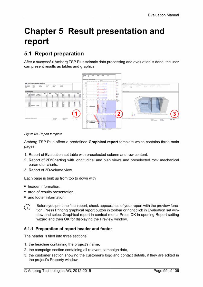
Evaluation Manual
© Amberg Technologies AG, 2012-2015 Page 99 of 106
Chapter 5 Result presentation andreport5.1 Report preparationAfter a successful Amberg TSP Plus seismic data processing and evaluation is done, the usercan present results as tables and graphics.
Figure 69. Report template
Amberg TSP Plus offers a predefined Graphical report template which contains three mainpages:
1. Report of Evaluation set table with preselected column and row content.2. Report of 2D/Charting with longitudinal and plan views and preselected rock mechanical
parameter charts.3. Report of 3D-volume view.
Each page is built up from top to down with
■ header information,■ area of results presentation,■ and footer information.
Before you print the final report, check appearance of your report with the preview func-tion. Press Printing graphical report button in toolbar or right click in Evaluation set win-dow and select Graphical report in context menu. Press OK in opening Report settingwizard and then OK for displaying the Preview window.
5.1.1 Preparation of report header and footer
The header is tiled into three sections:
1. the headline containing the project's name,2. the campaign section containing all relevant campaign data,3. the customer section showing the customer's logo and contact details, if they are edited in
the project's Property window.

Result presentation and report Evaluation Manual
Page 100 of 106 © Amberg Technologies AG, 2012-2015
Figure 70. Report header
Project related information The Name of project is taken from the Project tree. Youcan edit the given name in the property window of the mainproject tree node.
Campaign related information All campaign and processing related information are list-ed here. The campaign header resumes the entries of theproperty window content of the campaign node, like Acqui-sition date, Face and Reference tunnelmeter, Campaignname, heading direction, overburden, processing nameand operator's name. The report date is automatically setas print date.
Customer related information If available, the customer's information, like address and lo-go, can be displayed here. You can edit the information inthe property window of the main project tree node.
The footer is reserved for application and user's company information.
Figure 71. Report footer
Software version In the left part of the footer area, the currently installed software versionis listed.
Software owner Software owner information is displayed here as sender address. Edityour information and logo in the Options dialog in the File menu Gen-eral and Labels.
5.1.2 Preparation of result table
Depending on the result content which should be included into the report, the user can selectprinted rows and column. Due to the list and label template restriction of column width, theuser can reduce column content of Evaluation set table to main relevant information. The pre-selection of visible rows and columns should be done in the Evaluation set editor before thegraphical report is printed.
Units formatting Units, formats and number of decimals presented in the tableand graphic views have to be customized in the File Optionmenu Preferences.
Intersection axis The results can be presented as Local distance or Tunnelme-ter stationing. Select preferred stationing in the Evaluation setoption window, go to tab Rendering and select between Localdistances or Tunnelmeter.
Visible table content By default, all columns and rows of the reflector table will beprinted in the report. In the Evaluation set Option window, con-tent can be adjusted by user. Open the tab Reflector table inthe Option window:
Evaluation Manual Result presentation and report
© Amberg Technologies AG, 2012-2015 Page 101 of 106
Visible rows in table: In case you have muted reflectors in thetable, click the check box Hide muted reflectors. The rowsof muted reflectors will not be listed in the table and printedin the report.
Visible columns in table: Select the columns to show in thereport by checks.
5.1.3 Preparation of charts and 2D view
The charts with rock mechanical properties can be selected independently of result table con-tent. The selected charts will be listed in the upper part of the report page. In the lower part the2D longitudinal and plan views are shown with reflector color shading as previously set.
Charts selection Select preferred charts in the Evaluation set option window,go to tab Charts and set checks of the charts you want toshow in report. You may adjust the Coloring options and/orAxis options of selected charts for proper appearance.
2D view reflector color shad-ing
For presentation of the results in 2D longitudinal and planview one selection for color shading can be done. User canpresent the result based on a rock mechanical parameter oron the defined rock type color shading. Select the preferredcolor shading in the Evaluation set option window, go totab Rendering and select the base for the Reflector colorshading. Additionally, select color shading of each reflectoror of the defined border is possible.
5.1.4 Preparation of 3D view
The 3D window shows the already excavated tunnel tube from the reference location to thetunnel face with a tunnel profile as you have defined in the Tunnel model. It also shows thecorrect receiver and shot point locations with their defined azimuth and tilt angles. The selectedreflectors show a fixed defined size placed around the tunnel axis depending on the processingmodel size. They are bounded by a grey vertical and horizontal grid being defined by zoomposition, automatically. Their colour depends on selected color shading as in the 2D window.
3D volume position You need to adjust the camera position in the 3D view of the Eval-uation set. Rotate and zoom the volume into position you want topresent.
5.2 Printing graphical reportAfter the preparation of the report is finished the final print-out can be generated. AmbergTSP Plus offers several print-out formats and export functions. The print process is realized bywizards where the user is able to adjust result print-out appearance.

Result presentation and report Evaluation Manual
Page 102 of 106 © Amberg Technologies AG, 2012-2015
5.2.1 Report settings wizard
Figure 72. Report settings wizard
Charts range The range in direction of stationing is defined as default between the Startand End tunnelmeter of the processed model size. The shown Start and Endtunnelmeter depend on the selected general stationing in the tab Renderingof the Option window. An individual sector range can be defined here.
Charts scale The definition of print scale is related to the stationing axis of the charts and2D views and additionally to the vertical and horizontal axis in the longitudi-nal and plan axis.
5.2.2 Print options wizard
Figure 73. Print options wizard
Print target List of installed printers with selection of printer's setup.Direct to... By default Preview option is set. Press Start button to go to the preview of
report.
Amberg TSP plus offers many output formats in the drop down menu.
5.2.2.1 Printing formats
Amberg TSP plus offers many output formats in the drop down menu Direct to...:
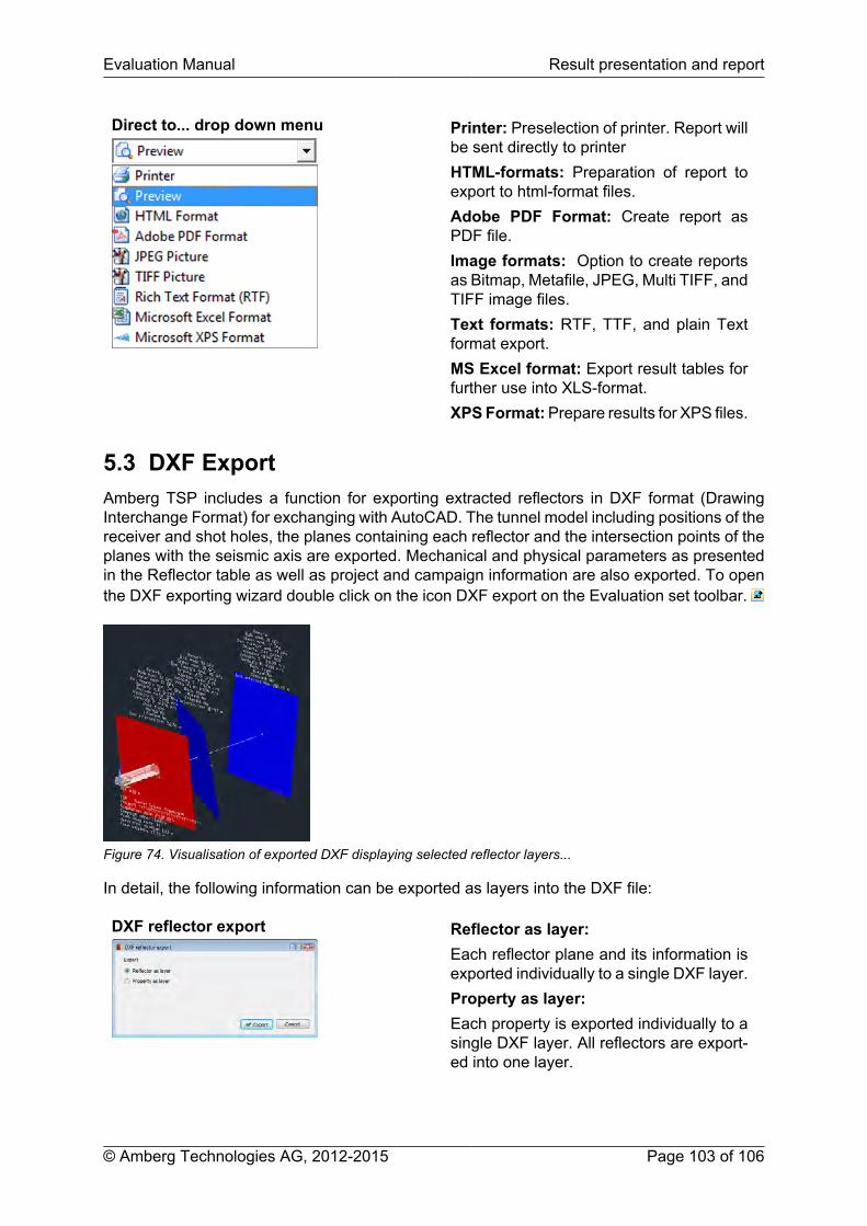
Evaluation Manual Result presentation and report
© Amberg Technologies AG, 2012-2015 Page 103 of 106
Direct to... drop down menu Printer: Preselection of printer. Report willbe sent directly to printerHTML-formats: Preparation of report toexport to html-format files.Adobe PDF Format: Create report asPDF file.Image formats: Option to create reportsas Bitmap, Metafile, JPEG, Multi TIFF, andTIFF image files.Text formats: RTF, TTF, and plain Textformat export.MS Excel format: Export result tables forfurther use into XLS-format.XPS Format: Prepare results for XPS files.
5.3 DXF ExportAmberg TSP includes a function for exporting extracted reflectors in DXF format (DrawingInterchange Format) for exchanging with AutoCAD. The tunnel model including positions of thereceiver and shot holes, the planes containing each reflector and the intersection points of theplanes with the seismic axis are exported. Mechanical and physical parameters as presentedin the Reflector table as well as project and campaign information are also exported. To openthe DXF exporting wizard double click on the icon DXF export on the Evaluation set toolbar.
Figure 74. Visualisation of exported DXF displaying selected reflector layers...
In detail, the following information can be exported as layers into the DXF file:
DXF reflector export Reflector as layer:Each reflector plane and its information isexported individually to a single DXF layer.Property as layer:Each property is exported individually to asingle DXF layer. All reflectors are export-ed into one layer.

Page 104 of 106


Amberg Technologies AGTrockenloostrasse 218105 RegensdorfSwitzerland
Phone: +41 44 870 92 22Mail: [email protected]://www.amberg.ch/at