Embed Size (px)
DESCRIPTION
etedg
Citation preview

Approved Methods
for the Modelling and Assessment of Air Pollutants in New South Wales

About this publication
Prepared by the NSW Environment Protection Authority (EPA), which is part of the Department of Environment and Conservation NSW (DEC).
For technical inquiries about this document, contact the Air Technical Advisory Services Unit of DEC.
Revision history
First published in NSW Government Gazette of 17 August 2001, p. 6109.
This revision appeared in NSW Government Gazette of 26 August 2005.
DEC is pleased to allow this material to be reproduced in whole or in part, provided the meaning is unchanged and DEC is acknowledged as the source, publisher and author of the material.
Published by: Department of Environment and Conservation 59–61 Goulburn Street, Sydney NSW 2000 PO Box A290, Sydney South NSW 1232 Tel: (02) 9995 5000 (switch) Tel: 131 555 (information and publications) Fax: (02) 9995 5999 Email: [email protected] Website: www.environment.nsw.gov.au
DEC 2005/361 ISBN 1 74137 488 X August 2005

Contents
1. Introduction............................................................................................... 1
1.1 Objective ............................................................................................................................ 1 1.2 Overview ............................................................................................................................ 1
2. Methodology overview............................................................................. 2
2.1 Different levels of assessment ............................................................................................ 2 2.2 Impact assessment methodology ........................................................................................ 2 2.3 Bibliography....................................................................................................................... 3
3. Emissions inventory................................................................................. 5
3.1 Identify all sources of air pollution and potential emissions .............................................. 5 3.2 Determine source release parameters ................................................................................. 6 3.3 Estimate emission rates ...................................................................................................... 6 3.4 Calculate emission concentration for point sources ........................................................... 7 3.5 Assess compliance with the Regulation ............................................................................. 7 3.6 Presentation of emissions inventory................................................................................... 8 3.7 Bibliography....................................................................................................................... 9
4. Meteorological data................................................................................ 10
4.1 Minimum data requirements ............................................................................................ 10 4.2 Siting and operating meteorological monitoring equipment ............................................ 10 4.3 Preparation of Level 1 meteorological data...................................................................... 11 4.4 Preparation of Level 2 meteorological data...................................................................... 16 4.5 Developing site-representative meteorological data using prognostic meteorological models ................................................................................ 16 4.6 Availability of meteorological processing software, guidance documents and prognostic meteorological models................................................................................... 17 4.7 Bibliography..................................................................................................................... 17
5. Background air quality terrain, sensitive receptors and building wake effects ................................................................................. 19
5.1 Background air quality data ............................................................................................. 19 5.2 Terrain and sensitive receptors......................................................................................... 20 5.3 Building wake effects....................................................................................................... 20 5.4 Bibliography..................................................................................................................... 20
6. Dispersion modelling ............................................................................. 21
6.1 Dispersion models ............................................................................................................ 21 6.2 Approved dispersion models ............................................................................................ 21 6.3 Advanced dispersion models for specialist application.................................................... 22 6.4 Dispersion modelling methodology using AUSPLUME ................................................. 23 6.5 Dispersion modelling methodology using CALPUFF ..................................................... 24 6.6 Calculate peak concentrations .......................................................................................... 24
6.7 Availability of dispersion modelling software and guidance documents......................... 25 6.8 Bibliography..................................................................................................................... 26
7. Interpretation of dispersion modelling results .................................... 27
7.1 SO2, NO2, O3, Pb, PM10, TSP, deposited dust, CO and HF.............................................. 28 7.2 Individual toxic air pollutants........................................................................................... 29 7.3 Complex mixtures of toxic air pollutants ......................................................................... 34 7.4 Individual odorous pollutants ........................................................................................... 35 7.5 Complex mixtures of odorous air pollutants .................................................................... 37 7.6 Presentation of assessment results.................................................................................... 38 7.7 What if impact assessment criteria are exceeded?............................................................ 38 7.8 Bibliography..................................................................................................................... 39
8. Modelling pollutant transformations..................................................... 41
8.1 Nitrogen dioxide assessment ............................................................................................ 41 8.2 Detailed assessment of ozone and nitrogen dioxide......................................................... 44 8.3 Bibliography..................................................................................................................... 44
9. Impact assessment report ..................................................................... 46
9.1 Site plan............................................................................................................................ 46 9.2 Description of the activities carried out on the site .......................................................... 46 9.3 Emissions inventory ......................................................................................................... 46 9.4 Meteorological data.......................................................................................................... 47 9.5 Background air quality data ............................................................................................. 47 9.6 Dispersion modelling ....................................................................................................... 47 9.7 Bibliography..................................................................................................................... 48
10. Emission limits ..................................................................................... 49
10.1 Legislation...................................................................................................................... 49 10.2 How does the EPA set emission limits in environment protection licences?................. 49 10.3 What information does the EPA use to set emission limits?.......................................... 50
11. Worked examples ................................................................................. 51
11.1 Developing site-specific emission limits........................................................................ 51 11.2 Dealing with elevated background concentrations......................................................... 52
12. Conversion factors............................................................................... 55
13. Glossary ................................................................................................ 57

Approved Methods for the Modelling and Assessment of Air Pollutants in New South Wales
1
1. Introduction
1.1 Objective This document, the Approved Methods for the Modelling and Assessment of Air Pollutants in New South Wales (‘Approved Methods’), lists the statutory methods for modelling and assessing emissions of air pollutants from stationary sources in the state. It is referred to in Part 4: Emission of Air Impurities from Activities and Plant in the Protection of the Environment Operations (Clean Air) Regulation 2002 (the ‘Regulation’). Industry has an obligation to ensure compliance with the requirements specified in the Regulation.
This document may also be referred to in conditions attached to statutory instruments, such as:
• licences or notices issued under the Protection of the Environment Operations Act 1997
• NSW Department of Environment and Conservation (DEC) Director General’s requirements under Part 4 of the Environmental Planning and Assessment Act 1979.
The procedures and methodologies contained in this document will undergo regular review, coinciding with the five-yearly review of the Regulation required by the Subordinate Legislation Act 1989.
1.2 Overview This document covers:
• preparation of emissions inventory data
• preparation of meteorological data
• methods for accounting for background concentrations and dealing with elevated background concentrations
• dispersion modelling methodology
• interpretation of dispersion modelling results
• impact assessment criteria for –
sulfur dioxide (SO2), nitrogen dioxide (NO2), ozone (O3), lead (Pb), PM10, total suspended particulates (TSP), deposited dust, carbon monoxide (CO) and hydrogen fluoride (HF)
individual and complex mixtures of toxic air pollutants
individual and complex mixtures of odorous air pollutants
• modelling of chemical transformation
• procedures for developing site-specific emission limits, including hydrogen sulfide as specified in clause 31 of the Regulation as amended
• worked examples.

Approved Methods for the Modelling and Assessment of Air Pollutants in New South Wales
2
2. Methodology overview
2.1 Different levels of assessment The two levels of impact assessment are:
• Level 1 – screening-level dispersion modelling technique using worst-case input data
• Level 2 – refined dispersion modelling technique using site-specific input data.
The impact assessment levels are designed so that the impact estimates from the second level should be more accurate than the first. This means that, for a given facility, the result of a Level 1 impact assessment would be more conservative and less specific than the result of a Level 2 assessment. It is not intended that an assessment should routinely progress through the two levels. If air quality impact is considered to be a significant issue, there is no impediment to immediately conducting a Level 2 assessment. Equally, if a Level 1 assessment conclusively demonstrates that adverse impacts will not occur, there is no need to progress to Level 2.
2.2 Impact assessment methodology There are five main stages in an air quality impact assessment:
1. Input data collection
2. Dispersion modelling
3. Processing dispersion model output data
4. Interpretation of dispersion modelling results
5. Preparation of an impact assessment report.
2.4.1 Input data collection
The first stage in the impact assessment is the collection of all the information required to complete the dispersion modelling. This includes development of an air emissions inventory; compilation of meteorological data; background air quality data; and terrain data. Sections 3, 4 and 5 of these Approved Methods detail the EPA’s requirements regarding the air quality impact assessment input data.
The development of the emissions inventory is one of the most important components of the impact assessment process. The inventory provides detailed information about all sources of air pollution at a premises. Emissions from the premises must be demonstrated to comply with the requirements of the Regulation before progressing through the other stages of the air quality impact assessment.
2.4.2 Dispersion modelling
AUSPLUME v. 6.0 is the approved dispersion model for use in most applications in NSW. However it is not approved in some applications where other more advanced dispersion models, such as CALPUFF and TAPM, may be more appropriate. The dispersion model input file should be prepared in accordance with the requirements of Section 6 of these Approved Methods and using the data collected in stage 1 of the impact assessment.

Approved Methods for the Modelling and Assessment of Air Pollutants in New South Wales
3
2.4.3 Processing dispersion model output data
Stage 3 of the assessment process is the prediction ground-level concentrations (glcs) of pollutants in the region surrounding the premises. The predicted glcs of all pollutants must be in the same units and for the same averaging period as the relevant impact assessment criteria. The EPA’s impact assessment criteria, together with the requirements regarding the presentation of the predicted glcs, are specified in Section 7.6.
2.4.4 Interpretation of dispersion modelling results
Stage 4 of the impact assessment is the interpretation of the dispersion modelling results. The predicted glcs are compared with the EPA’s impact assessment criteria and compliance indicates the proposal is unlikely to result in adverse air quality impacts.
If a premises does not comply with the impact assessment criteria, the assessment must be revised to incorporate additional control or mitigation measures. To determine incremental increases in the cost of air pollution abatement, a sensitivity analysis can be carried out by varyin g:
• source release parameters
• separation distance
• efficiency of pollution control equipment
• level of management practice.
The results can be used to select the most cost-effective and environmentally effective control strategy.
2.4.5 Preparation of an impact assessment report
Stage 5 of the impact assessment is the preparation of a report. The air quality impact assessment report must be prepared in accordance with the requirements specified in Section 9 of these Approved Methods.
2.3 Bibliography Earth Tech 2000, A User’s Guide for the CALPUFF Dispersion Model (Version 5), Earth Tech Incorporated, Long Beach CA, USA.
Earth Tech 2000, A User’s Guide for the CALMET Meteorological Model (Version 5), Earth Tech Incorporated, Long Beach CA, USA.
EPA Victoria 1985, Plume Calculation Procedure: An Approved Procedure under Schedule E of State Environment Protection Policy (The Air Environment), Publication 210, Environment Protection Authority of Victoria, Melbourne.
EPA Victoria 1986, The AUSPLUME Gaussian Plume Dispersion Model, First Edition, Publication 264, Environment Protection Authority of Victoria, Melbourne.
EPA Victoria 1999, AUSPLUME Gaussian Plume Dispersion Model: Technical User Manual, Publication 671, Environment Protection Authority of Victoria, Melbourne.
EPA Victoria 2000, AUSPLUME Gaussian Plume Dispersion Model: Technical User Manual, Environment Protection Authority of Victoria, Melbourne.
Hurley, P. 2005, The Air Pollution Model (TAPM) Version 3: User Manual, CSIRO Atmospheric Research Technical Paper No. 31, CSIRO Division of Atmospheric Research, Melbourne.

Approved Methods for the Modelling and Assessment of Air Pollutants in New South Wales
4
USEPA 1999, Guideline on Air Quality Models, 40 CFR, Chapter I, Part 51, Appendix W, United States Environmental Protection Agency, Washington DC, USA.

Approved Methods for the Modelling and Assessment of Air Pollutants in New South Wales
5
3. Emissions inventory The emissions inventory is the foundation of the air quality impact assessment. Developing a sound emissions inventory should be a priority task and requires the collation of a significant amount of data. A thorough air emissions inventory for a premises identifies all sources of air pollution, the air pollutants emitted from each source, and estimates the emission concentration and rate of all air pollutants emitted. The following section provides guidance on each step of the development of an emissions inventory.
3.1 Identify all sources of air pollution and potential emissions A thorough understanding of the premises is essential in developing an emissions inventory. Undertaking a site visit of the existing premises or a detailed review of the engineering drawings for the proposed premises is necessary to identify all sources of air pollution and gain an understanding of the process and industry. This knowledge can be supplemented with a literature review on the industry and its most prevalent air pollution issues.
For all sources of air pollution at a premises, identify the following:
• release type
• location (in metres relative to fixed origin, elevation and discharge geometry)
• potential air pollutants emitted.
3.1.1 Release type
Source configuration may be one of the following types:
Point sources
For a point source, emissions emanate from a very small opening such as a stack or vent. Stacks usually emit hot gases forcefully into the atmosphere at a fixed height above ground level.
Tall point sources: The term ‘tall’ point source usually refers to sources that protrude out of the surface boundary layer (e.g. over 30 to 50 m tall).
Wake-affected point sources: Where nearby buildings interfere with the trajectory and growth of the plume, the source is called a wake-affected point source. A point source is wake-affected if stack height is less than or equal to 2.5 times the height of buildings located within a distance of 5L (where L is the lesser of the height or width of the building) from each release point.
Wake-free point sources: Wake-free point sources are more than 2.5 times the height of the largest nearby building, so that surrounding buildings do not influence the stack top airflow.
Area sources
An area source has a more realistic two-dimensional structure but only a limited vertical extent. It is a source with a large surface area such as a liquid surface (pond, lagoon) or a landfill surface.
Line sources
A line source is a special case of a long, thin area source. In practice, these sources are taken to be at ground level and thin. A line source becomes an area source if the breadth exceeds 20% of the length.

Approved Methods for the Modelling and Assessment of Air Pollutants in New South Wales
6
Volume sources
A volume source is an essentially three-dimensional structure. Usually there are a sufficient number of emission points to consider a uniform emission rate over the full source structure. They are diffuse sources, such as emissions from within a building.
3.2 Determine source release parameters For proposed premises this information is obtained from the engineering drawings and plans. For existing premises, this information can be obtained from site-specific sampling and analysis. The release parameters for each source type are:
Point: stack height, stack diameter, temperature, discharge velocity, moisture, pressure, carbon dioxide and oxygen concentration
Diffuse area: surface area, side length and release height
Diffuse volume: side length, release height, and initial horizontal and vertical plume spread (σy and σz).
3.3 Estimate emission rates There are a number of methods that can be used to estimate the emission rate from each source. The EPA’s preferred methods are direct measurement for existing sources and manufacturers’ design specifications for proposed sources. Emission factors are generally used when there is no other information available or when emissions can reasonably be demonstrated to be negligible.
3.3.1 Manufacturers’ design specifications or performance guarantees
Manufacturers’ design specifications or performance guarantees can be used to estimate the emission rate of air pollutants from proposed sources. Such specifications provide a reliable means of determining the upper limit to the emission rate or concentration of air pollutants for sources that are maintained and operated in a proper and efficient manner.
Post-commissioning testing may be required to establish that sources comply with the manufacturers’ design specifications and/or performance guarantees.
3.3.2 Direct measurement
For sources where manufacturers’ design specifications or performance guarantees are unknown, emission rates and source release parameters should normally be established from the results of source emission sampling and analysis. All sampling of source emissions and analysis of air pollutants must be in accordance with Section 1 of the Approved Methods for the Sampling and Analysis of Air Pollutants in New South Wales (DEC 2005).
3.3.3 Emission factors
An emission factor is usually an equation that relates the quantity of a pollutant released to process throughput. These factors are generally averages of all available data of acceptable quality, and are generally assumed to be representative of long-term averages for all facilities in the source category. As stated above, emission factors are generally used when there is no other information available or when emissions can reasonably be demonstrated to be negligible. Some databases of emission factors include:
• US EPA’s AP-42 Emissions Factors (www.epa.gov/ttn/chief)

Approved Methods for the Modelling and Assessment of Air Pollutants in New South Wales
7
• National Pollutant Inventory Emissions Estimation Technique Manuals (www.npi.gov.au/handbooks/approved_handbooks/sector-manuals.html).
3.3.4 Accounting for variability in emission rates
If the source is large, the frequency distribution of emission rates should be compiled and used in conjunction with the frequency distribution of meteorological conditions to predict the overall frequency distribution of predicted glcs. Manufacturers’ design specifications or performance guarantees can be useful for establishing the upper bounds of likely operational variability.
If the source is smaller and data is available to describe the distribution of emission rates, use the 99.9th percentile.
If no data is available to describe the distribution of emission rates, use the maximum measured or calculated emission rate.
Where practicable, emission rate data should be constructed using an averaging period that is the lesser of one hour or the sampling time used in the concentration calculations.
3.4 Calculate emission concentration for point sources The concentration of a pollutant emitted from a source is calculated using equation 3.1:
Equation 3.1
FRER
C ii =
where:
iC = the concentration of pollutant i emitted from a source in mg/m3
iER = the rate pollutant i is emitted from the source in mg/s
FR = the gaseous volumetric flow rate in m3/s
The inventory should contain two emission concentrations:
1. Actual concentration of a pollutant emitted from a source (mg/Am3) calculated using the actual gaseous volumetric flow rate (Am3/s) and measured emission rate in Equation 3.1
2. Concentration of a pollutant emitted from a source corrected to the reference conditions as specified in the Regulation (mg/Nm3 @ O2%). This is calculated using the gaseous volumetric flow rate corrected to normal conditions (dry, 273K, 101.3 kPa) and the measured emission rate in Equation 3.1. The emission concentration (in mg/Nm3) is then corrected to the appropriate oxygen reference condition. Further guidance on correcting to reference and equivalent values is provided in DEC (2005).
3.5 Assess compliance with the Regulation The inventory must be used to demonstrate compliance with the Regulation. All sources of air emissions must comply with the requirements of the Regulation. If a source does not comply, the emissions inventory must be revised to reflect the implementation of new technology and/or pollution control equipment that will comply with the Regulation.

Approved Methods for the Modelling and Assessment of Air Pollutants in New South Wales
8
3.6 Presentation of emissions inventory The results of the emissions inventory must be presented to include the following information:
• all release parameters of stack and fugitive sources (e.g. temperature, exit velocity, stack dimensions, flow rate, moisture content, pressure, carbon dioxide and oxygen concentration)
• pollutant emission concentrations and a comparison against the relevant requirements of the Regulation.
A suggested format for summarising and presenting the results of the emissions inventory in the impact assessment report is provided in Tables 3.1 and 3.2. The additional data that should be included in the impact assessment report for complex mixtures of odour and hydrogen sulfide is included in Table 3.3.
Table 3.1: Stack source release parameters
Sour
ce
Rel
ease
ty
pe
Stac
k he
ight
(m
)
Exit
tem
p.
(o C)
Exit
diam
eter
(m
)
Exit
velo
city
(m
/s)
Oxy
gen
conc
. (%
)
Moi
stur
e co
nten
t (%
)
Flow
rate
(A
m3 /s
)
Flow
rate
(N
m3 /s
)
Boiler No. 1
Wake-affected
20 150 4 15 10 15 188.5 103.4
Table 3.2: Stack emission concentrations and regulation limits
Pollutant
Emission rate (g/s)
Emission concentration
(mg/Am3)
Corrected emission
concentration (mg/Nm3 at stack
reference conditions)
Regulation emission
concentration limit (mg/Nm3 at stack reference
conditions)
Sulfur dioxide 40 212.2 N/A N/A
Solid particles 2 10.6 31.6 100
Oxides of nitrogen
15 79.6 237.4 350
Table 3.3: Peak odour emission rates
Peak odour emission rate (OUm3/s)
Source
Source type
Odour emission rate (OUm3/s)
Stability class Near-field Far-field
A, B, C, D 50,000 46,000 Lagoon No. 1 Area 20,000
E, F 46,000 38,000

Approved Methods for the Modelling and Assessment of Air Pollutants in New South Wales
9
3.7 Bibliography DEC 2005, Approved Methods for the Sampling and Analysis of Air Pollutants in New South Wales, Department of Environment and Conservation NSW, Sydney.
EPA 2001, Draft Policy: Assessment and Management of Odour from Stationary Sources in NSW, NSW Environment Protection Authority, Sydney.
EPA 2001, Technical Notes – Draft Policy: Assessment and Management of Odour from Stationary Sources in NSW, NSW Environment Protection Authority, Sydney.
EPA Victoria 1985, Plume Calculation Procedure: An Approved Procedure under Schedule E of State Environment Protection Policy (The Air Environment), Publication 210, Environment Protection Authority of Victoria, Melbourne.
EPA Victoria 1990, The AUSPLUME Gaussian Plume Dispersion Model, First Edition, Publication 264, Environment Protection Authority of Victoria, Melbourne.
EPA Victoria 1999, AUSPLUME Gaussian Plume Dispersion Model: Technical User Manual, Publication 671, Environment Protection Authority of Victoria, Melbourne.
EPA Victoria 2000, AUSPLUME Gaussian Plume Dispersion Model: Technical User Manual, Environment Protection Authority of Victoria, Melbourne.
Department of Environment and Heritage, National Pollutant Inventory Emissions Estimation Technique Manuals (www.npi.gov.au/handbooks/approved_handbooks/sector-manuals.html)
USEPA 1995, AP 42, Fifth Edition Compilation of Air Pollutant Emission Factors, Volume 1: Stationary Point and Area Sources (www.epa.gov/ttn/chief/ap42/index.html)

Approved Methods for the Modelling and Assessment of Air Pollutants in New South Wales
10
4. Meteorological data The meteorological data used in the dispersion model is of fundamental importance as it drives the transport and dispersion of the air pollutants in the atmosphere. The most critical parameters are wind direction, which determines the initial direction of transport of pollutants from their sources; wind speed, which dilutes the plume in the direction of transport and determines the travel time from source to receptor; and atmospheric turbulence, which indicates the dispersive ability of the atmosphere.
4.1 Minimum data requirements The meteorological data used in the dispersion modelling is one factor that determines the level of assessment.
Level 1 impact assessments are conducted using ‘synthetic’ worst-case meteorological data. Table 4.1 lists the wind speed and stability class combinations that need to be included in the synthetic worst-case meteorological data file.
Level 2 impact assessments are conducted using at least one year of site-specific meteorological data. The meteorological data must be 90% complete in order to be acceptable for use in Level 2 impact assessments (i.e. for one year, there can be no more than 876 hours of data missing). If site-specific meteorological data are not available for a Level 2 impact assessment, at least one year of site-representative meteorological data must be used. The site-representative data should be:
• preferably collected at a meteorological monitoring station. Where measured data is unavailable or of insufficient quality for dispersion modelling purposes, a meteorological data file may be generated using a prognostic meteorological model such as TAPM (Section 4.5).
• correlated against a longer-duration site-representative meteorological database of at least five years (preferably five consecutive years) to be deemed acceptable. It must be clearly established that the data adequately describes the expected meteorological patterns at the site under investigation (e.g. wind speed, wind direction, ambient temperature, atmospheric stability class, inversion conditions and katabatic drift).
4.2 Siting and operating meteorological monitoring equipment The following methods specified in DEC (2005) must be used for establishing, siting, operating and maintaining meteorological monitoring equipment:
• AM-1 (Standards Australia 1987a)
• AM-2 (Standards Australia 1987b)
• AM-4 (USEPA 2000).
All meteorological stations used to collect data for dispersion modelling purposes must use an anemometer that has a stall speed of 0.5 m/s or less.
For the AUSPLUME dispersion model, the meteorological parameters required are:
• wind speed (m/s)
• wind direction (°)
• ambient temperature (°C)
• atmospheric stability class
Approved Methods for the Modelling and Assessment of Air Pollutants in New South Wales
11
• mixed layer height (m).
For deposited dust, the data file should include hourly average values for the following additional parameters:
• Monin–Obukhov length (m)
• surface friction velocity (m/s)
• surface roughness height (m).
Wind speed, wind direction and ambient temperature can be directly measured, but atmospheric stability class and mixed layer height need to be determined indirectly using other meteorological parameters with empirical formulae.
A meteorological station needs to measure and electronically log wind speed, wind direction and ambient temperature. In addition, for determining atmospheric stability class, one of the following is required:
• cloud cover and cloud ceiling height by visual observations obtained from the Bureau of Meteorology
• total solar radiation measured in conjunction with temperature at two levels and electronically logged
• sigma theta (the standard deviation of the horizontal wind direction fluctuation) electronically logged.
All parameters must be logged as 1-hour average values as a minimum requirement. In some circumstances these variables may need to be averaged and logged at intervals of 10 minutes or less.
4.3 Preparation of Level 1 meteorological data DEC’s preferred methods for the preparation of synthetic meteorological data are specified below. The use of methods other than these should be discussed with the Air Technical Advisory Services Unit of DEC.
4.3.1 Wind speed and stability class
Gaussian plume dispersion models use stability categories as indicators of atmospheric turbulence and the dispersive properties of the atmosphere. Based on the work of Pasquill and Gifford, seven stability categories have been defined: A – very unstable; B – unstable; C – slightly unstable; D – neutral; E – slightly stable; F – stable; and G – very stable conditions. In most dispersion models, stability classes F and G are combined into one class, F.
The stability class at any given time depends on:
• static stability (vertical temperature profile of the atmosphere, i.e. migrating high and low air-pressure masses)
• convective or thermal turbulence (caused by the rising of air heated at ground level)
• mechanical turbulence (a function of wind speed and surface roughness, i.e. wind flow over rough terrain, trees or buildings).
Table 4.1 lists the minimum wind speed and stability class combinations that must be included in a Level 1 meteorological data file.

Approved Methods for the Modelling and Assessment of Air Pollutants in New South Wales
12
Table 4.1: Wind speed and stability class combinations for a Level 1 data file
Wind speed (m/s)
Stability class
0.5
1
1.5
2
2.5
3
3.5
4
4.5
5
6
7
8
10
12
14
16
18
20
A * * * * * *
B * * * * * * * * * *
C * * * * * * * * * * * * * *
D * * * * * * * * * * * * * * * * * * *
E * * * * * * * * * *
F * * * * * *
4.3.2 Ambient temperature
For Level 1 impact assessments, the maximum and minimum ambient temperatures that are representative of the site must be included in the Level 1 meteorological data file to account for the range in possible plume rise. Higher ambient temperatures will result in the lowest plume rise and hence the largest impacts.
4.3.3 Mixing height
For Level 1 impact assessments, the mixing height for neutral and unstable conditions (classes A–D) can be calculated using an estimate of the mechanically driven mixing height. The mechanical mixing height, h, can be calculated as follows:
Equation 4.1: Mechanical mixing height for stability classes A–D
h = 0.3 × u* / f
where:
h = mixing height (m)
u* = friction velocity (m/s)
f = coriolis parameter
For Level 1 impact assessments, the mixing height, h, for stable conditions (classes E and F) can either be set at an unlimited value (e.g. 5000 m) or calculated as follows:
Equation 4.2: Mechanical mixing height for stability classes E and F
h = 0.4 × (u*L / f)0.5
where:
h = mixing height (m)
u* = friction velocity (m/s)
L = Monin–Obukhov length (m)
F = coriolis parameter
4.3.4 Monin–Obukhov length
The Monin–Obukhov length, L, characterises the stability of the surface layer. The surface layer is defined as the layer above the ground in which the vertical variation of heat and momentum flux is negligible. The surface layer is typically 10% the height of the mixed

Approved Methods for the Modelling and Assessment of Air Pollutants in New South Wales
13
layer. The parameter, L, can be calculated using the linear approximation to Golder’s plot (Golder 1972) as follows:
Equation 4.3: Monin–Obukhov length
1/L = X + Y × log10 (Zo)
where:
L = Monin–Obukhov length (m)
X & Y = parameters dependent on the Pasquill–Gifford stability class (see Table 4.2)
Zo = surface roughness height (m) (see Table 4.3)
Table 4.2: Parameterisation of Golder’s plot
Pasquill–Gifford stability class
Parameter A B C D E F
X –0.096 –0.037 –0.002 0.000 0.004 0.035
Y 0.029 0.025 0.018 0.000 –0.018 –0.0365 In Equation 4.3:
• the value of Zo is the surface roughness height, unless the surface roughness height is outside the range Zomin to Zomax presented in Table 4.3
• if the surface roughness height < Zomin use the value of Zomin for Zo
• if the surface roughness > Zomax use the value of Zomax for Zo.
Table 4.3: Upper and lower limits for surface roughness heights for each Pasquill–Gifford stability class
Pasquill–Gifford stability class
Parameter A B C D E F
Zomin 0.001 0.001 0.001 0.001 0.001 0.001
Zomax 18.0 30.0 1.25 50.0 1.6 9.0 Table 4.4 presents typical values of surface roughness height for various land uses.
Table 4.4: Typical values of surface roughness height for various land-use categories (AUSPLUME version 6.0)
Land-use category
Roughness height Zo (m)
Land-use category
Roughness height Zo (m)
Hill 2.0 High-rise 1.0
Industrial area 0.8 Commercial 0.8
Forest 0.8 Residential 0.4
Rolling rural 0.4 Flat rural 0.1
Flat desert 0.01 Water 0.0001

Approved Methods for the Modelling and Assessment of Air Pollutants in New South Wales
14
4.3.5 Surface friction velocity
The surface friction velocity, u*, is a measure of mechanical turbulence and is directly related to the surface roughness. The parameter, u*, can be calculated using the procedure presented below (Businger and Fleagle 1980; McRae 1981).
Condition 1: Wind speed = 0
u* = 0.001 m/s
Condition 2: Unstable conditions (Pasquill–Gifford stability classes A, B or C, or 1/L < 0)
u* = VK × Wsp / φ
where:
u* = surface friction velocity (m/s)
VK = von Karman constant; use a value of 0.4
Wsp = absolute value of the wind speed at height Zr (m/s)
φ = calculated according to the following equation:
φ = ln (Zr / Zo) + ln ((PZo2 + 1.0) × (PZo + 1.0)2 / ((PZr
2 + 1.0) × (PZr + 1.0)2)) + 2 × (tan–1(PZr) – tan–1(PZo))
where:
Zr = reference height for the wind measurements (m)
Zo = surface roughness height (m)
PZo and PZr = calculated according to the following equations:
PZr = (1.0 – 15.0 × Zr / L)0.25
PZo = (1.0 – 15.0 × Zo / L) 0.25
Zr = reference height for the wind measurements (m)
Zo = surface roughness height (m)
L = Monin–Obukhov length (m)
Condition 3: Neutral conditions (Pasquill–Gifford stability class D, or 1/L = 0)
u* = VK × Wsp / ln (Zr/Zo)
where:
u* = surface friction velocity (m/s)
VK = von Karman constant; use a value of 0.4
Wsp = absolute value of the wind speed at height Zr (m/s)
Zr.= reference height for the wind measurements (m)
Zo = surface roughness height (m)
Condition 4: Stable conditions (Pasquill–Gifford stability class E or F, or 1/L > 0)
u* = VK × Wsp / (ln (Zr / Zo) + 4.7 / L × (Zr – Zo))
where:
u* = surface friction velocity (m/s)
VK = von Karman constant; use a value of 0.4

Approved Methods for the Modelling and Assessment of Air Pollutants in New South Wales
15
Wsp = absolute value of the wind speed at height Zr (m/s)
Zr = reference height for the wind measurements (m)
Zo = surface roughness height (m)
4.3.6 Coriolis parameter
The coriolis parameter accounts for variation in wind direction with height (wind shear) at different latitudes and can be calculated in accordance with well-established techniques. The coriolis parameter, f, can be calculated as follows:
f = 2Ωsin(φ)
where:
Ω = Earth’s rotation rate (2π/86400 or 7.29 × 10⁻⁵ rad·s–1)
π = pi or 3.1416 radians (rad)
86400 = number of seconds in the day (s/day)
φ = latitude in radians (rad)
Table 4.5 lists an example of typical mixing heights for a location with a similar latitude to Sydney (34°) and in a rural location (surface roughness height of 0.3 m) to be included in the Level 1 meteorological data file.
Table 4.5: Typical mixing heights for a rural location (km)
Wind speed (m/s) Stability
class
0.5 1
1.5
2
2.5
3
3.5
4
4.5
5
6
7
8
10
12
14
16
18
20
A 0.2 0.4 0.6 0.8 1.0 1.2
B 0.2 0.4 0.5 0.7 0.9 1.0 1.2 1.4 1.6 1.8
C 0.2 0.3 0.5 0.6 0.8 0.9 1.1 1.2 1.4 1.5 1.8 2.1 2.4 3.1
D 0.2 0.3 0.4 0.6 0.7 0.8 1.0 1.1 1.3 1.4 1.7 2.0 2.2 2.8 3.3 3.9 4.5 5.0 5.0
E 5.0 5.0 5.0 5.0 5.0 5.0 5.0 5.0 5.0 5.0
F 5.0 5.0 5.0 5.0 5.0 5.0 5.0
Table 4.6 lists an example of typical mixing heights for a location with a similar latitude to Sydney (34°) and in an urban location (surface roughness height of 1.0 m) to be included in the Level 1 meteorological data file.
Table 4.6: Typical mixing heights for an urban location (km)
Wind speed (m/s) Stability
class
0.5 1
1.5
2
2.5
3
3.5
4
4.5
5
6
7
8
10
12
14
16
18
20
A 0.3 0.6 1.0 1.3 1.6 2.0
B 0.3 0.5 0.8 1.1 1.4 1.7 1.9 2.2 2.5 2.7
C 0.2 0.4 0.7 0.9 1.1 1.3 1.5 1.8 2.0 2.2 2.6 3.1 3.5 4.4
D 0.2 0.4 0.6 0.8 1.1 1.3 1.5 1.7 1.9 2.1 2.6 2.9 3.4 4.3 5.0 5.0 5.0 5.0 5.0
E 5.0 5.0 5.0 5.0 5.0 5.0 5.0 5.0 5.0 5.0
F 5.0 5.0 5.0 5.0 5.0 5.0 5.0

Approved Methods for the Modelling and Assessment of Air Pollutants in New South Wales
16
4.4 Preparation of Level 2 meteorological data For guidance on processing meteorological data for dispersion modelling purposes, the USEPA guide (USEPA 2000) and USEPA processor (USEPA 1996) should be used.
4.4.1 Stability class
In order of preference, the following methods outlined in USEPA (2000) should be used to determine stability class:
Turner’s 1964 method: This requires information on solar altitude or zenith angle, cloud cover, cloud ceiling height and wind speed. Solar altitude can easily be calculated, but cloud cover and ceiling height are generally determined through visual observations.
Solar radiation–delta temperature method: This retains the basic structure and rationale of Turner’s 1964 method but eliminates the need for observations of cloud cover and ceiling height. The method uses the surface-layer wind speed (measured at 10 m) in combination with measurements of total solar radiation during the day and a low-level vertical temperature difference (i.e. at 2 m and 10 m) at night.
Sigma theta method (the standard deviation of the horizontal wind direction fluctuation): All modern meteorological data loggers include software to determine sigma theta.
For Level 2 impact assessments, hourly stability class should be estimated using the USEPA meteorological pre-processor for regulatory models (USEPA 1996) or a processor that includes similar techniques.
4.4.2 Mixing height
Mixing height is the depth through which pollutants released to the atmosphere are typically mixed by dispersive processes. Dispersion of pollutants in the lower atmosphere is greatly aided by the convective and turbulent mixing that takes place. Mixing height determines the vertical extent of dispersion for releases occurring below that height. Releases occurring above that height are assumed to have no ground-level impact (with the exception of fumigation episodes). Therefore, the greater the vertical extent of the mixed layer, the larger the volume available to dilute pollutant emissions.
Morning and afternoon mixing heights are estimated using vertical temperature profiles (otherwise known as ‘upper air data’) and surface temperature measurements. For Level 2 impact assessments, hourly mixing heights should be estimated from the twice-daily mixing height values, sunrise and sunset times, and hourly stability categories by using the USEPA meteorological pre-processor for regulatory models (USEPA 1996) or a processor which includes similar techniques.
4.5 Developing site-representative meteorological data using prognostic meteorological models In some areas of NSW neither site-specific nor site-representative meteorological data are available that are suitable for use in regulatory dispersion modelling applications. Where this is the case, prognostic meteorological models may be used.
CSIRO’s TAPM (Hurley 2005a and 2005b; Hurley et al. 2005) is a three-dimensional prognostic meteorological and dispersion modelling system. TAPM is the most frequently used prognostic meteorological model in NSW. TAPM uses databases of terrain, vegetation, soil type, sea surface temperature and synoptic-scale meteorological analyses for Australia. TAPM is driven by 6-hourly synoptic analyses at approximately 75-kilometre resolution. This

Approved Methods for the Modelling and Assessment of Air Pollutants in New South Wales
17
database is derived from Local Area Prediction System analysis data from the Bureau of Meteorology.
The following model set-up is the minimum specification that must be used to generate a meteorological data file for regulatory dispersion modelling applications:
• TAPM v. 2.0 or later
• GEODATA 9-second (~250 m) terrain height database
• TAPM default databases for land use, synoptic analyses and sea surface temperature
• 25 by 25 horizontal grid points
• 25 vertical levels
• outer grid of 30 kilometres, with nesting grids of 10 km, 3 km and 1 km
• TAPM defaults for advanced meteorological inputs.
4.6 Availability of meteorological processing software, guidance documents and prognostic meteorological models Meteorological processing software and guidance documents can be electronically downloaded, free of charge, from the USEPA website: www.epa.gov/ttn/scram/
TAPM can be purchased from CSIRO and includes a terrain and land-use database CD and synoptic analysis databases for two calendar years for Australia. Data for other geographical regions can be purchased together with extra synoptic analyses for other calendar years and a finer-resolution terrain (9-second digital elevation model) dataset for Australia.
4.7 Bibliography Businger, J. and Fleagle, R. 1980, An Introduction to Atmospheric Physics, Academic Press, New York.
DEC 2005, Approved Methods for the Sampling and Analysis of Air Pollutants in New South Wales, Department of Environment and Conservation NSW, Sydney.
Golder, D. 1972, ‘Relations among stability parameters in the surface layer’, Boundary Layer Meteorology 3, 47–58.
Hurley, P. 2005a, The Air Pollution Model (TAPM) Version 3, Part 1: Technical Description, CSIRO Atmospheric Research Technical Paper No. 71, CSIRO Division of Atmospheric Research, Melbourne.
Hurley, P. 2005b, The Air Pollution Model (TAPM) Version 3: User Manual, CSIRO Atmospheric Research Technical Paper No. 31, CSIRO Division of Atmospheric Research, Melbourne.
Hurley, P., Physick, W., Luhar, A. and Edwards, M. 2005, The Air Pollution Model (TAPM) Version 3, Part 2: Summary of Some Verification Studies, CSIRO Atmospheric Research Technical Paper No. 72, CSIRO Division of Atmospheric Research, Melbourne.
McRae, G.J. 1981, Mathematical Modelling of Photochemical Air Pollution, Chapter 4, ‘Turbulent Diffusion Coefficients’, PhD Thesis, California Institute of Technology, Los Angeles.
Standards Australia 1987a, AS 2922–1987, Ambient Air – Guide for the Siting of Sampling Units, Standards Australia, Sydney.

Approved Methods for the Modelling and Assessment of Air Pollutants in New South Wales
18
Standards Australia 1987b, AS 2923–1987, Ambient Air – Guide for the Measurement of Horizontal Wind for Air Quality Applications, Standards Australia, Sydney.
USEPA 1996, Meteorological Processor for Regulatory Model (MPRM), User’s Guide, EPA-454/B-96-002, United States Environmental Protection Agency, Washington DC, USA.
USEPA 2000, Meteorological Monitoring Guidance for Regulatory Modelling Applications, EPA-450/R-99-005, United States Environmental Protection Agency, Washington DC, USA.
Zanetti, P. 1990, Air Pollution Modelling: Theories, Computational Methods and Available Software, Van Nostrand Reinhold, New York.
Approved Methods for the Modelling and Assessment of Air Pollutants in New South Wales
19
5. Background air quality, terrain, sensitive receptors and building wake effects
5.1 Background air quality data Including background concentrations of pollutants in the assessment enables the total impact of the proposal (i.e. impact of emissions on existing air quality) to be assessed. The background concentrations of air pollutants are ideally obtained from ambient monitoring data collected at the proposed site. As this is extremely rare, data is typically obtained from a monitoring site as close as possible to the proposed location where the sources of air pollution resemble the existing sources at the proposal site.
5.1.1 Accounting for background concentrations
For impact assessments of sulfur dioxide (SO2), nitrogen dioxide (NO2), ozone (O3), PM10, total suspended particulates (TSP), deposited dust, lead (Pb), carbon monoxide (CO) and hydrogen fluoride (HF), the existing background concentrations of the pollutants in the vicinity of the proposal should be included in the assessment as follows:
Level 1 assessments
• Obtain ambient monitoring data that includes at least one year of continuous measurements.
• Determine the maximum background concentration of the pollutant being assessed for each relevant averaging period.
• At the maximum exposed off-site receptor, add the maximum background concentration and the 100th percentile dispersion model prediction to obtain the total impact for each averaging period.
Level 2 assessments
• Obtain ambient monitoring data that includes at least one year of continuous measurements and is contemporaneous with the meteorological data used in the dispersion modelling.
• At each receptor, add each individual dispersion model prediction to the corresponding measured background concentration (e.g. add the first hourly average dispersion model prediction to the first hourly average background concentration) to obtain hourly predictions of total impact.
• At each receptor, determine the 100th percentile total impact for the relevant averaging.
The use of an approach other than those above should be discussed with the Air Technical Advisory Services Unit of DEC.
5.1.2 Sourcing ambient monitoring data
Ambient monitoring data from a variety of locations in NSW is published in DEC’s Quarterly Air Monitoring Reports (www.environment.nsw.gov.au/air/datareports.htm) and may be of assistance in characterising the existing ambient air quality. Data may also be obtained from various industry monitoring programs.
All monitoring to establish background concentrations must be conducted in accordance with the methods specified in DEC (2005).

Approved Methods for the Modelling and Assessment of Air Pollutants in New South Wales
20
5.1.3 Dealing with elevated background concentrations
In some locations, existing ambient air pollutant concentrations may exceed the impact assessment criteria from time to time. In such circumstances, a licensee must demonstrate that no additional exceedances of the impact assessment criteria will occur as a result of the proposed activity and that best management practices will be implemented to minimise emissions of air pollutants as far as is practical. Refer to the worked example included in Section 11.2.
5.2 Terrain and sensitive receptors The dispersion modelling input file requires information regarding the surrounding terrain and sensitive receptors. Terrain and receptor files are developed which include the location and height in metres relative to a fixed origin. The location of any particularly sensitive receptors (and likely future sensitive receptors) such as residences, schools and hospitals can also be specifically included in the receptor file.
5.3 Building wake effects PRIME is the EPA’s preferred building wake algorithm. AUSPLUME v. 6.0 includes the PRIME building wake algorithm and the Building Profile Input Program (BPIP) for entering the location and dimension of buildings. The location and dimensions of buildings located within a distance of 5L (where L is the lesser of the height or width of the building) from each release point for buildings with a height greater than 0.4 times the stack height should be entered in BPIP.
5.4 Bibliography DEC 2005, Approved Methods for the Sampling and Analysis of Air Pollutants in New South Wales, Department of Environment and Conservation NSW, Sydney.
DEC 4th Quarter 2003–present, Quarterly Air Quality Monitoring Report Part A: DEC Data, Department of Environment and Conservation NSW, Sydney.
DEC 4th Quarter 2003–present, Quarterly Air Quality Monitoring Report Part B: Industry Data, Department of Environment and Conservation NSW, Sydney.
EPA 1992–3rd Quarter 2003, Quarterly Air Quality Monitoring Report Part A: EPA Data, NSW Environment Protection Authority, Sydney.
EPA 1992–3rd Quarter 2003, Quarterly Air Quality Monitoring Report Part B: Industry Data, NSW Environment Protection Authority, Sydney.
EPA Victoria 2000, AUSPLUME Gaussian Plume Dispersion Model: Technical User Manual, Environment Protection Authority of Victoria, Melbourne.
Schulman, L.L., Strimaitis, D.G. and Scire, J.S. 1998, Development and Evaluation of the PRIME Plume Rise and Building Downwash Model, Preprint Volume for the Tenth Joint Conference on Applications of Air Pollution Meteorology with A&WMA, American Meteorological Society, Phoenix, Arizona.
SPCC 1975–1991, Quarterly Air Quality Monitoring Reports, State Pollution Control Commission, Sydney.
USEPA 1995, User’s Guide to the Building Profile Input Program, Revised February 1995, PA-454/R-93-038, United States Environmental Protection Agency, Washington DC, USA.

Approved Methods for the Modelling and Assessment of Air Pollutants in New South Wales
21
6. Dispersion modelling
6.1 Dispersion models Dispersion models provide the ability to mathematically simulate atmospheric conditions and behaviour. They are used to calculate spatial and temporal sets of concentrations and particle deposition due to emissions from various sources. Dispersion models can be used to determine the affected zone around an emitter by producing results that can be compared against impact assessment criteria.
Dispersion models can provide concentration or deposition estimates over an almost unlimited grid of user-specified locations, and can be used to evaluate both existing and forecast emission scenarios. In this capacity, air dispersion modelling is a useful tool in assessing the air quality impacts associated with existing and proposed emission sources. The results of the dispersion modelling analysis can be used to develop control strategies that should ensure compliance with the assessment criteria. Dispersion models can also be used to estimate the cumulative impacts of various industries that are located close to one another.
Dispersion models are widely used by environmental regulators in Australia, New Zealand, the United States, the United Kingdom and Europe, and industry well understands their limitations. The results have been shown, through numerous model evaluation studies, to be sufficiently robust to be relied on to calculate concentration limits for point-source stack emissions.
6.2 Approved dispersion models AUSPLUME v. 6.0 or later is the approved dispersion model for use in most simple, near-field applications in NSW, where coastal effects and complex terrain are of no concern.
AUSPLUME is a Gaussian plume model, based on the assumption that cross-sections through elevated plumes from point sources of pollution have a Gaussian (or normal) distribution of concentration. AUSPLUME is also a steady-state model, which assumes the atmosphere is in a state of uniform flow, and wind velocity is a function of height alone and does not vary with direction. The mathematical basis of AUSPLUME is the Victorian EPA’s Plume Calculation Procedure (EPA Victoria 1985), which itself is an extension of the ISC model (USEPA 1995).
AUSPLUME v. 6.0 or later is specifically not approved for use in the following applications:
• complex terrain, non-steady-state conditions: AUSPLUME is a steady-state model and is unable to adjust the winds to reflect the effects of terrain. The straight-line trajectory assumption of the plume model is unable to handle the curved flow associated with terrain-induced deflection of channelling. AUSPLUME should not be used for terrain where the height of any receptor exceeds the lowest release height.
• buoyant line plumes (e.g. discharges from the roof vents of aluminium smelters)
• coastal effects such as fumigation: AUSPLUME is unable to consider large changes in meteorological conditions which can occur over short distances across a coastline.
• high frequency of stable calm night-time conditions: Pollutants can accumulate under such conditions or will flow downwind with the drainage flow. AUSPLUME has no memory of the previous hour’s weather conditions as each hour is treated independently of the next and material is carried away instantaneously, to the edge of the grid, even if only light winds are prevailing.

Approved Methods for the Modelling and Assessment of Air Pollutants in New South Wales
22
• high frequency of calm conditions: AUSPLUME cannot handle calm conditions because of the inverse wind speed dependence plume equation. AUSPLUME assumes a minimum wind speed, which shoots the plume out to the edge of the grid even though the plume may not have moved at all.
• inversion break-up fumigation conditions.
There are also other situations where another dispersion model may be more scientifically sound than AUSPLUME. In these instances, CALPUFF or TAPM (Section 6.3) may be appropriate. The two key factors that should be considered in evaluating whether to use a conventional plume model, such as AUSPLUME, or a more sophisticated approach are:
1. Is the steady-state assumption in the plume model valid?
2. Do the technical parameterisations in the plume model adequately treat the situation to be modelled?
For other applications, the choice of a dispersion model other than AUSPLUME, CALPUFF or TAPM should be discussed with the Air Technical Advisory Services Unit of DEC. For the calculation of site-specific emission limits for hydrogen sulfide and sulfur dioxide, written approval must be obtained from the EPA for the use of a dispersion model other than AUSPLUME, CALPUFF or TAPM. The application must show that the alternative dispersion model is scientifically sound for the proposed application.
6.3 Advanced dispersion models for specialist application In circumstances where the AUSPLUME dispersion model is not approved or suitable for use, other dispersion models may be appropriate. Guidance on choosing appropriate alternative dispersion models can be found in the USEPA publication Guideline on Air Quality Models (USEPA 1999). CALPUFF and TAPM are the most commonly used alternative dispersion models for regulatory dispersion modelling applications in NSW. However only experienced and appropriately trained professionals should use them.
6.3.1 CALPUFF
CALPUFF is a multi-layer, multi-species, non-steady-state Gaussian puff dispersion model that is able to simulate the effects of time- and space-varying meteorological conditions on pollutant transport. This enables the model to account for a variety of effects such as spatial variability of meteorological conditions, causality effects, dry deposition and dispersion over a variety of spatially varying land surfaces, plume fumigation, low wind speed dispersion, pollutant transformation and wet removal. CALPUFF has various algorithms for parameterising dispersion processes, including the use of turbulence-based dispersion coefficients derived from similarity theory or observations.
CALPUFF has been accepted by the USEPA as a guideline model to be used in regulatory applications involving the long-range transport of pollutants (> 50 km). It can also be used on a case-by-case basis in situations involving complex flow and non-steady-state cases up to 50 kilometres from the source.
CALPUFF v. 5.7, CALMET v. 5.5 and CALPOST v. 5.4 or later should be used.

Approved Methods for the Modelling and Assessment of Air Pollutants in New South Wales
23
6.3.2 TAPM
The Air Pollution Model (TAPM) was developed by the CSIRO to simulate three-dimensional meteorology and pollution dispersion in areas where meteorological data are sparse or non-existent. The modelling system contains a number of dispersion modules. These include a particle/puff dispersion model for dispersion from point, line, area and volume sources, and a three-dimensional grid-point model for urban air pollution studies. The dispersion models allow for plume rise and building wake effects, wet and dry deposition and photochemistry for urban airshed applications. TAPM v. 2.0 or later should be used.
6.4 Dispersion modelling methodology using AUSPLUME Unless otherwise stated, the default options specified in the Technical Users Manual (EPA Victoria 2000) must be used with AUSPLUME. These options are the most appropriate for most impact assessment applications.
Terrain effects
• Use the Egan half-height approach to account for terrain effects.
Building wake effects
• All building dimensions must be entered in 10-degree increments. Use the USEPA utility program BPIP (USEPA 1995) within AUSPLUME to calculate the 36 wind-direction-dependent building dimensions.
• Use the PRIME method to account for building wake effects.
• The USEPA’s guidance document on good engineering practice (USEPA 1985) must be taken into account when designing new stacks to avoid building wake effects.
Horizontal dispersion curves
• For stacks < 100 m high, use sigma theta values or Pasquill–Gifford curves.
• For stacks > 100 m high, use Briggs rural curves.
Vertical dispersion curves
• For stacks < 100 m high, use Pasquill–Gifford curves.
• For stacks > 100 m high, use Briggs rural curves.
‘Enhance plume spreads for buoyancy’
• Enable this option for both the horizontal and vertical dimensions.
‘Adjust Pasquill–Gifford formulae for roughness height’
• Use this option.
Plume rise parameters
• Use the AUSPLUME defaults.
Wind speed categories
• Use the AUSPLUME defaults.
Wind profile exponents
• Use Irwin rural wind profile exponents for rural areas.
• Use Irwin urban wind profile exponents for urban areas.

Approved Methods for the Modelling and Assessment of Air Pollutants in New South Wales
24
6.5 Dispersion modelling methodology using CALPUFF CALPUFF includes an option to automatically set all the options to the USEPA default values. These include:
• Wind speed profile: ISC Rural
• Transitional plume rise modelled
• Stacktip downwash
• Partial plume penetration
• Dispersion curves: Pasquill–Gifford or dispersion coefficients using turbulence-based micro-meteorology
• No adjustment of dispersion curves for roughness
• Terrain: partial plume adjustment method
6.6 Calculate peak concentrations The evaluation of odour impacts requires the estimation of short or peak concentrations on the time scale of less than one second. Dispersion model predictions are typically valid for averaging periods of one hour and longer. Dispersion models, such as AUSPLUME, therefore need to be supplemented to accurately simulate atmospheric dispersion of odours and the instantaneous perception of odours by the human nose.
The prediction of peak concentrations from estimates of ensemble means can be obtained from a ratio between extreme short-term concentration and longer-term averages. Properly defined peak-to-mean ratios depend upon the type of source, atmospheric stability and distance downwind. Table 6.1 shows the EPA-recommended factors for estimating peak concentrations for different source types, stabilities and distances as developed by Katestone Scientific (1995 and 1998).
The P/M60 ratios in Table 6.1 are for an idealised situation for one source in flat terrain where the receptor is located along the centreline of the single plume. The ratios do not consider fluctuations away from the centre line, terrain influences or plume interaction from multiple sources.
The EPA requires peak ground-level concentrations to be calculated for the following pollutants:
• hydrogen sulfide
• complex mixtures of odour.
A screening level assessment of peak glcs can be undertaken by applying the ratios in Table 6.1 to multiple sources at a premises. These ratios can be applied to the emission rates entered into the dispersion model as follows:
1. Determine the source type, stability class and if the receptors are near-field or far-field or both.
2. Select the appropriate P/M60 ratios from Table 6.1.
3. For wake-affected point sources, determine the meteorological conditions (i.e. wind speed and stability class) under which the source is wake-affected and wake-free.
4. Apply P/M60 ratios to odour and hydrogen sulfide emission rates so they vary with wind speed and stability class.

Approved Methods for the Modelling and Assessment of Air Pollutants in New South Wales
25
More detailed procedures for estimating peak glcs from multiple sources are discussed in Katestone Scientific (1995 and1998).
Table 6.1: Factors for estimating peak concentrations in flat terrain (Katestone Scientific 1995 and 1998)
Source type
Pasquill–Gifford stability class
Near-field P/M60*
Far-field P/M60*
A, B, C, D 2.5 2.3 Area
E, F 2.3 1.9
Line A–F 6 6
Surface wake-free point
A, B, C 12 4
D, E, F 25 7
Tall wake-free point
A, B, C 17 3
D, E, F 35 6
Wake-affected point
A–F 2.3 2.3
Volume A–F 2.3 2.3
* Ratio of peak 1-second average concentrations to mean 1-hour average concentrations
6.7 Availability of dispersion modelling software and guidance documents Windows-based AUSPLUME v. 6.0 can be purchased by writing to:
Environment Protection Authority of Victoria 27 Francis Street Melbourne Victoria 3000
The BPIP PRIME (BPIPPRM) user’s manual and software can be electronically downloaded, free of charge, from the USEPA website at www.epa.gov/scram001/tt22.htm#bpipprm
The CALPUFF dispersion modelling package and guidance documents can be electronically downloaded, free of charge, from the Earth Tech Incorporated website at earthtec.vwh.net/download/download.htm
The TAPM software can be purchased by writing to:
Dr Peter Hurley CSIRO Atmospheric Research PMB 1 Aspendale Victoria 3195
Guidance documents and information about TAPM can be obtained from the CSIRO website at www.dar.csiro.au/tapm/
Other dispersion modelling software and guidance documents can be electronically downloaded free of charge from the USEPA website at www.epa.gov/ttn/scram/

Approved Methods for the Modelling and Assessment of Air Pollutants in New South Wales
26
6.8 Bibliography Earth Tech 2000, A User’s Guide for the CALPUFF Dispersion Model (Version 5), Earth Tech Incorporated, Long Beach CA, USA.
Earth Tech 2000, A User’s Guide for the CALMET Meteorological Model (Version 5), Earth Tech Incorporated, Long Beach CA, USA.
EPA Victoria 1985, Plume Calculation Procedure, Environment Protection Authority of Victoria, Melbourne.
EPA Victoria 1986, The AUSPLUME Gaussian Plume Dispersion Model, First Edition, Publication 264, Environment Protection Authority of Victoria, Melbourne.
EPA Victoria 1999, AUSPLUME Gaussian Plume Dispersion Model: Technical User Manual, Publication 671, Environment Protection Authority of Victoria, Melbourne.
EPA Victoria 2000, AUSPLUME Gaussian Plume Dispersion Model: Technical User Manual, Environment Protection Authority of Victoria, Melbourne.
Hurley, P. 2005, The Air Pollution Model (TAPM) Version 3, Part 1: Technical Description, CSIRO Atmospheric Research Technical Paper No. 71, CSIRO Division of Atmospheric Research, Melbourne.
Hurley, P. 2005, The Air Pollution Model (TAPM) Version 3: User Manual, CSIRO Atmospheric Research Technical Paper No. 31, CSIRO Division of Atmospheric Research, Melbourne.
Hurley, P., Physick, W., Luhar, A. and Edwards, M. 2005, The Air Pollution Model (TAPM) Version 3, Part 2: Summary of Some Verification Studies, CSIRO Atmospheric Research Technical Paper No. 72, CSIRO Division of Atmospheric Research, Melbourne.
Katestone Scientific 1995, The Evaluation of Peak-to-Mean Ratios for Odour Assessments, volumes I and II, Katestone Scientific Pty Ltd, Brisbane.
Katestone Scientific 1998, Peak-to-Mean Concentration Ratios for Odour Assessments, Katestone Scientific Pty Ltd, Brisbane.
Schulman, L.L., Strimaitis, D.G. and Scire, J.S. 1998, Development and Evaluation of the PRIME Plume Rise and Building Downwash Model, Preprint Volume for the Tenth Joint Conference on Applications of Air Pollution Meteorology with A&WMA, American Meteorological Society, Phoenix, Arizona, 1998.
USEPA 1985, Guideline for Determination of Good Engineering Practice Stack Height (Technical Support Document for the Stack Height Regulations), Revised, EPA-450/4-80-023R, United States Environmental Protection Agency, Washington DC, USA.
USEPA 1995, User’s Guide to the Building Profile Input Program, Revised February 1995, EPA-454/R-93-038, United States Environmental Protection Agency, Washington DC, USA.
USEPA 1995, User’s Guide for the Industrial Source Complex (ISC3) Dispersion Models, Volume 1 and Volume 2, US EPA Office of Air Quality Planning and Standards Emissions, Monitoring, and Analysis Division Research Triangle Park, North Carolina.
USEPA 1997, Addendum to ISC3 User’s Guide, The PRIME Plume Rise and Building Downwash Model, United States Environmental Protection Agency, Washington DC, USA.
USEPA 1999, Guideline on Air Quality Models, 40 CFR, Chapter I, Part 51, Appendix W, United States Environmental Protection Agency, Washington DC, USA.

Approved Methods for the Modelling and Assessment of Air Pollutants in New South Wales
27
7. Interpretation of dispersion modelling results The primary purpose of an air quality impact assessment is to determine whether emissions from a premises will comply with the appropriate environmental outcomes. The assessment criteria outlined below reflect the environmental outcomes adopted by the EPA.
To ensure the environmental outcomes are achieved, emissions from a premises must be assessed against the assessment criteria. The cumulative impact of emissions from several facilities also needs to be considered. Impacts of sulfur dioxide (SO2), nitrogen dioxide (NO2), ozone (O3), Lead (Pb), particles (PM10), total suspended particulates (TSP), deposited dust, carbon monoxide (CO) and hydrogen fluoride (HF) must be combined with existing background levels before comparison with the relevant impact assessment criteria.
Assessment criteria must not be used as limit conditions in environment protection licences. Compliance with assessment criteria (i.e. in the ambient air at the boundary of the premises or nearest sensitive receptor) cannot be readily determined for regulatory purposes. For point sources, a site-specific stack emission limit can be calculated (see Section 10 and 11.1) so that the assessment criteria will not be exceeded at and beyond the boundary of a premise because of emissions from those sources.

Approved Methods for the Modelling and Assessment of Air Pollutants in New South Wales
28
7.1 SO2, NO2, O3, Pb, PM10, TSP, deposited dust, CO and HF
7.1.1 Impact assessment criteria
Table 7.1: Impact assessment criteria for SO2, NO2, O3, Pb, PM10, TSP, deposited dust, CO and HF
Concentration Pollutant Averaging period pphm µg/m3
Source
10 minutes 25 712 NHMRC (1996)
1 hour 20 570 NEPC (1998)
24 hours 8 228 NEPC (1998)
Sulfur dioxide (SO2)
Annual 2 60 NEPC (1998)
1 hour 12 246 NEPC (1998) Nitrogen dioxide (NO2) Annual 3 62 NEPC (1998)
1 hour 10 214 NEPC (1998) Photochemical oxidants (as ozone)
4 hours 8 171 NEPC (1998)
Lead Annual – 0.5 NEPC (1998)
24 hours – 50 NEPC (1998) PM10
Annual – 30 EPA (1998)
Total suspended particulates (TSP)
Annual – 90 NHMRC (1996)
g/m2/montha g/m2/monthb
Deposited dustc Annual 2 4 NERDDC (1988) ppm mg/m3
15 minutes 87 100 WHO (2000)
1 hour 25 30 WHO (2000)
Carbon monoxide (CO)
8 hours 9 10 NEPC (1998) µg/m3 d µg/m3 e
90 days 0.5 0.25 ANZECC (1990)
30 days 0.84 0.4 ANZECC (1990)
7 days 1.7 0.8 ANZECC (1990)
Hydrogen fluoride
24 hours 2.9 1.5 ANZECC (1990)
a Maximum increase in deposited dust level. b Maximum total deposited dust level. c Dust is assessed as insoluble solids as defined by AS 3580.10.1–1991 (AM-19). d General land use, which includes all areas other than specialised land use. e Specialised land use, which includes all areas with vegetation sensitive to fluoride, such as grape vines and stone fruits.

Approved Methods for the Modelling and Assessment of Air Pollutants in New South Wales
29
7.1.2 Application of impact assessment criteria
The assessment criteria in Table 7.1 must be applied as follows:
1. At the nearest existing or likely future off-site sensitive receptor.
2. The incremental impact (predicted impacts due to the pollutant source alone) for each pollutant must be reported in units and averaging periods consistent with the impact assessment criteria.
3. Background concentrations must be included using the procedures specified in Section 5.
4. Total impact (incremental impact plus background) must be reported as the 100th percentile in concentration or deposition units consistent with the impact assessment criteria and compared with the relevant impact assessment criteria.
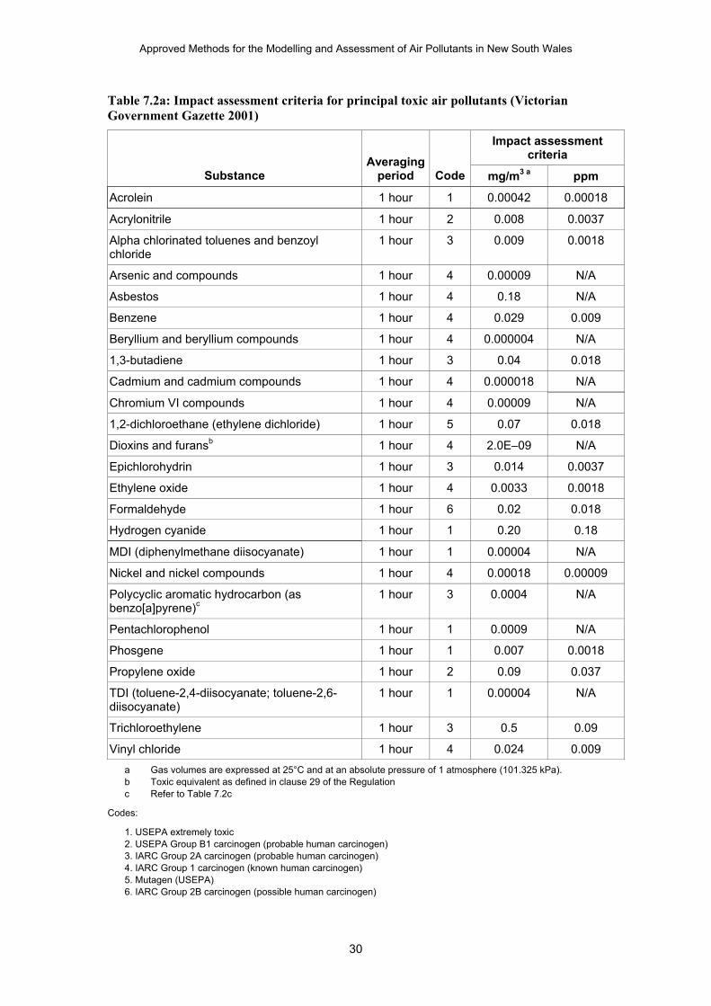
7.2 Individual toxic air pollutants
7.2.1 Impact assessment criteria
Tables 7.2a and 7.2b list the impact assessment criteria for individual toxic air pollutants. The principal toxic air pollutants in Table 7.2a are defined on the basis that they are carcinogenic, mutagenic, teratogenic, highly toxic or highly persistent in the environment. Criteria for other individual toxic air pollutants are shown in Table 7.2b.
Principal toxic air pollutants must be minimised to the maximum extent achievable through the application of best-practice process design and/or emission controls. Decisions with respect to achievability will have regard to technical, logistical and financial considerations. Technical and logistical considerations include a wide range of issues that will influence the feasibility of an option: for example, whether a particular technology is compatible with an enterprise’s production processes.
Financial considerations relate to the financial viability of an option. It is not expected that reductions in emissions should be pursued ‘at any cost’. Nor does it mean that the preferred option will always be the lowest cost option. However it is important that the preferred option is cost-effective. The costs need to be affordable in the context of the relevant industry sector within which the enterprise operates. This will need to be considered on a case-by-case basis through discussions with the EPA.
Approved Methods for the Modelling and Assessment of Air Pollutants in New South Wales
30
Table 7.2a: Impact assessment criteria for principal toxic air pollutants (Victorian Government Gazette 2001)
Impact assessment criteria
Substance
Averaging period
Code mg/m3 a ppm
Acrolein 1 hour 1 0.00042 0.00018
Acrylonitrile 1 hour 2 0.008 0.0037
Alpha chlorinated toluenes and benzoyl chloride
1 hour 3 0.009 0.0018
Arsenic and compounds 1 hour 4 0.00009 N/A
Asbestos 1 hour 4 0.18 N/A
Benzene 1 hour 4 0.029 0.009
Beryllium and beryllium compounds 1 hour 4 0.000004 N/A
1,3-butadiene 1 hour 3 0.04 0.018
Cadmium and cadmium compounds 1 hour 4 0.000018 N/A
Chromium VI compounds 1 hour 4 0.00009 N/A
1,2-dichloroethane (ethylene dichloride) 1 hour 5 0.07 0.018
Dioxins and furansb 1 hour 4 2.0E–09 N/A
Epichlorohydrin 1 hour 3 0.014 0.0037
Ethylene oxide 1 hour 4 0.0033 0.0018
Formaldehyde 1 hour 6 0.02 0.018
Hydrogen cyanide 1 hour 1 0.20 0.18
MDI (diphenylmethane diisocyanate) 1 hour 1 0.00004 N/A
Nickel and nickel compounds 1 hour 4 0.00018 0.00009
Polycyclic aromatic hydrocarbon (as benzo[a]pyrene)c
1 hour 3 0.0004 N/A
Pentachlorophenol 1 hour 1 0.0009 N/A
Phosgene 1 hour 1 0.007 0.0018
Propylene oxide 1 hour 2 0.09 0.037
TDI (toluene-2,4-diisocyanate; toluene-2,6-diisocyanate)
1 hour 1 0.00004 N/A
Trichloroethylene 1 hour 3 0.5 0.09
Vinyl chloride 1 hour 4 0.024 0.009
a Gas volumes are expressed at 25°C and at an absolute pressure of 1 atmosphere (101.325 kPa). b Toxic equivalent as defined in clause 29 of the Regulation c Refer to Table 7.2c
Codes:
1. USEPA extremely toxic 2. USEPA Group B1 carcinogen (probable human carcinogen) 3. IARC Group 2A carcinogen (probable human carcinogen) 4. IARC Group 1 carcinogen (known human carcinogen) 5. Mutagen (USEPA) 6. IARC Group 2B carcinogen (possible human carcinogen)
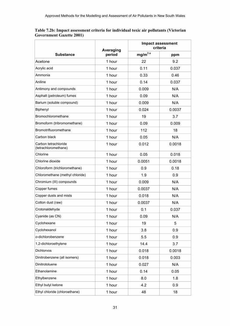
Approved Methods for the Modelling and Assessment of Air Pollutants in New South Wales
31
Table 7.2b: Impact assessment criteria for individual toxic air pollutants (Victorian Government Gazette 2001)
Impact assessment criteria
Substance
Averaging period mg/m3 a ppm
Acetone 1 hour 22 9.2
Acrylic acid 1 hour 0.11 0.037
Ammonia 1 hour 0.33 0.46
Aniline 1 hour 0.14 0.037
Antimony and compounds 1 hour 0.009 N/A
Asphalt (petroleum) fumes 1 hour 0.09 N/A
Barium (soluble compound) 1 hour 0.009 N/A
Biphenyl 1 hour 0.024 0.0037
Bromochloromethane 1 hour 19 3.7
Bromoform (tribromomethane) 1 hour 0.09 0.009
Bromotrifluoromethane 1 hour 112 18
Carbon black 1 hour 0.05 N/A
Carbon tetrachloride (tetrachloromethane)
1 hour 0.012 0.0018
Chlorine 1 hour 0.05 0.018
Chlorine dioxide 1 hour 0.0051 0.0018
Chloroform (trichloromethane) 1 hour 0.9 0.18
Chloromethane (methyl chloride) 1 hour 1.9 0.9
Chromium (III) compounds 1 hour 0.009 N/A
Copper fumes 1 hour 0.0037 N/A
Copper dusts and mists 1 hour 0.018 N/A
Cotton dust (raw) 1 hour 0.0037 N/A
Crotonaldehyde 1 hour 0.1 0.037
Cyanide (as CN) 1 hour 0.09 N/A
Cyclohexane 1 hour 19 5
Cyclohexanol 1 hour 3.8 0.9
o-dichlorobenzene 1 hour 5.5 0.9
1,2-dichloroethylene 1 hour 14.4 3.7
Dichlorvos 1 hour 0.018 0.0018
Dinitrobenzene (all isomers) 1 hour 0.018 0.003
Dinitrotoluene 1 hour 0.027 N/A
Ethanolamine 1 hour 0.14 0.05
Ethylbenzene 1 hour 8.0 1.8
Ethyl butyl ketone 1 hour 4.2 0.9
Ethyl chloride (chloroethane) 1 hour 48 18

Approved Methods for the Modelling and Assessment of Air Pollutants in New South Wales
32
Impact assessment criteria
Substance
Averaging period mg/m3 a ppm
Ethylene glycol (vapour) 1 hour 1 N/A
n-hexane 1 hour 3.2 0.9
2-hexanone 1 hour 1.8 0.46
Hydrogen chloride 1 hour 0.14 0.09
Iron oxide fumes 1 hour 0.09 N/A
Magnesium oxide fumes 1 hour 0.18 N/A
Maleic anhydride 1 hour 0.018 0.0046
Manganese and compounds 1 hour 0.018 N/A
Mercury organic 1 hour 0.00018 N/A
Mercury inorganic 1 hour 0.0018 N/A
Methyl acrylate 1 hour 0.66 0.18
Methyl bromide (bromomethane) 1 hour 0.35 0.09
Methylene chloride (dichloromethane) 1 hour 3.19 0.9
Nitric acid 1 hour 0.09 0.037
n-pentane 1 hour 33 11
2-pentanone 1 hour 12.8 3.7
Phthalic anhydride 1 hour 0.1 0.018
Propylene glycol monomethyl ether 1 hour 6.6 1.8
Silver metal 1 hour 0.0018 N/A
Silver, soluble compounds (as Ag) 1 hour 0.00018 N/A
Sulfuric acid 1 hour 0.018 N/A
1,1,1-trichloroethane (methyl chloroform)
1 hour 12.5 2.3
1,1,2-trichloroethane 1 hour 1.0 0.18
Trichlorofluoromethane 1 hour 103 18.3
Trimethylbenzene (mixed isomers) 1 hour 2.2 0.46
Vinyl toluene 1 hour 4.4 0.9
Welding fumes (total particulate) 1 hour 0.09 N/A
Wood dust hardwoods 1 hour 0.0018 N/A
Wood dust softwoods 1 hour 0.009 N/A
Zinc chloride fumes 1 hour 0.018 N/A
Zinc oxide fumes 1 hour 0.09 N/A
a Gas volumes are expressed at 25°C and at an absolute pressure of 1 atmosphere (101.325 kPa).

Approved Methods for the Modelling and Assessment of Air Pollutants in New South Wales
33
Table 7.2c: Potency equivalency factors (PEFs) for PAHs (OEHHA 1994)
PAH or derivative CAS number PEF
Benzo[a]pyrene 50-32-8 1
Benzo[a]anthracene 56-55-3 0.1
Benzo[b]fluoranthene 205-99-2 0.1
Benzo[j]fluoranthene 205-82-3 0.1
Benzo[k]fluoranthene 207-08-9 0.1
Bibenz[a,j]acridine 224-42-0 0.1
Bibenz[a,h]acridine 226-36-8 0.1
7h-dibenzo[c,g]carbazole 194-59-2 1
Dibenzo[a,e]pyrene 192-65-4 1
Dibenzo[a,h]pyrene 189-64-0 10
Dibenzo[a,i]pyrene 189-55-9 10
Dibenzo[a,l]pyrene 191-30-0 10
5-nitroacenaphthene 602-87-9 0.01
Indeno[1,2,3-cd]pyrene 193-39-5 0.1
5-methylchrysene 3697-24-3 1
1-nitropyrene 5522-43-0 0.1
4-nitropyrene 57835-92-4 0.1
1,6-dinitropyrene 42397-64-8 10
1,8-dinitropyrene 42397-65-9 1
6-nitrocrysene 7496-02-8 10
2-nitrofluorene 607-57-8 0.01
Chrysene 218-01-9 0.01
Dibenz[a,h]anthracene 53-70-3 0.4
7,12-dimethylbenzanthracene 57-97-6 21.8
3-methylcholanthrene 56-49-5 1.9

Approved Methods for the Modelling and Assessment of Air Pollutants in New South Wales
34
7.2.2 Application of impact assessment criteria
The impact assessment criteria for individual toxic air pollutants in Tables 7.2a and 7.2b must be applied as follows:
1. At and beyond the boundary of the facility.
2. The incremental impact (predicted impacts due to the pollutant source alone) for each pollutant must be reported in concentration units consistent with the criteria (mg/m3 or ppm), for an averaging period of 1 hour and as the:
a. 100th percentile of dispersion model predictions for Level 1 impact assessments, or
b. 99.9th percentile of dispersion model predictions for Level 2 impact assessments.
3. Polycyclic aromatic hydrocarbons (PAH) as benzo[a]pyrene (BaP) must be calculated using the potency equivalency factors for PAHs in Table 7.2c.
4. Dioxins and furans as toxic equivalent must be calculated according to the requirements of clause 29 of the Regulation.
7.3 Complex mixtures of toxic air pollutants
7.3.1 Risk assessment criteria
Where a number of toxic and carcinogenic air pollutants are emitted in significant amounts, demonstrating compliance with impact assessment criteria may not adequately demonstrate the protection of human health. A risk assessment can be used to assess the potential risk arising from exposure to emissions of toxic air pollutants after emissions of principal toxic air pollutants have been reduced to the maximum extent achievable, and compliance with the impact assessment criteria has been demonstrated. Health risk assessment is particularly useful for the assessment of multiple chemicals and exposure through multiple pathways (e.g. inhalation, ingestion or dermal adsorption).
Take care when interpreting the results of a risk assessment. A risk assessment does not demonstrate that a particular impact will happen. Often the information available to risk assessors is imperfect, and consequently assumptions are made that tend to overestimate a risk. It is legitimate for a risk assessor to go through a process of refining assumptions to obtain a more realistic assessment of risk.
Guidelines for undertaking risk assessment in Australia have been prepared by the enHealth Council (enHealth 2002). These guidelines provide a broad framework for risk assessment that aims to enhance its use in environmental impact assessment.
The risk assessment process includes the following aspects:
• hazard identification
• assessment of exposure
• dose response assessment
• risk characterisation.
Assessment of exposure should be based on enHealth’s published information on the assessment of exposure in Australia (enHealth 2001 and 2003).

Approved Methods for the Modelling and Assessment of Air Pollutants in New South Wales
35
Dose response assessment and risk characterisation can be undertaken in accordance with the following:
• The Air Toxics Hot Spots Program Guidance Manual for Preparation of Health Risk Assessments (OEHHA 2003)
• Hot Spots Analysis and Reporting Program (HARP) (CARB 2003a)
• Hot Spots Analysis and Reporting Program – User Guide Version 1.0 (CARB 2003b).
The results of the risk assessment should be compared with the criteria specified in Table 7.3 for carcinogenic risk and the acute and chronic non-carcinogenic hazard index.
Table 7.3: Acceptance criteria for risk and hazard index
Evaluation
Carcinogenic risk (CR)
Acute and chronic non-carcinogenic hazard index (HI)
Acceptable Less than 1 in 1 million (1 × 10⁻⁶)
Less than 0.2
Require best practice for air toxics and CR < 1 in 1 million and HI < 0.2
1 in 1 million to 1 in 10 thousand(1 × 10⁻⁶ to 1 × 10⁻⁴)
0.2 to 10
Not acceptable Greater than 1 in 10 thousand (1 × 10⁻⁴)
Greater than 10
7.4 Individual odorous air pollutants
7.4.1 Impact assessment criteria
Table 7.4a lists the impact assessment criteria for individual odorous air pollutants. Equation 7.1 must be used to select the appropriate impact assessment criterion for hydrogen sulfide as a function of population density:
Equation 7.1
Impact assessment criterion (µg/m3) = (log10 (population) – 4.5) / –0.87
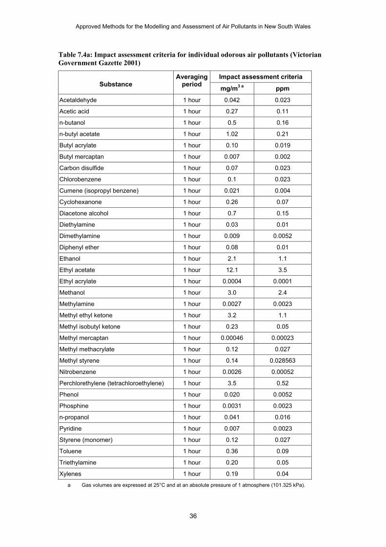
Approved Methods for the Modelling and Assessment of Air Pollutants in New South Wales
36
Table 7.4a: Impact assessment criteria for individual odorous air pollutants (Victorian Government Gazette 2001)
Impact assessment criteria Substance
Averaging period mg/m3 a ppm
Acetaldehyde 1 hour 0.042 0.023
Acetic acid 1 hour 0.27 0.11
n-butanol 1 hour 0.5 0.16
n-butyl acetate 1 hour 1.02 0.21
Butyl acrylate 1 hour 0.10 0.019
Butyl mercaptan 1 hour 0.007 0.002
Carbon disulfide 1 hour 0.07 0.023
Chlorobenzene 1 hour 0.1 0.023
Cumene (isopropyl benzene) 1 hour 0.021 0.004
Cyclohexanone 1 hour 0.26 0.07
Diacetone alcohol 1 hour 0.7 0.15
Diethylamine 1 hour 0.03 0.01
Dimethylamine 1 hour 0.009 0.0052
Diphenyl ether 1 hour 0.08 0.01
Ethanol 1 hour 2.1 1.1
Ethyl acetate 1 hour 12.1 3.5
Ethyl acrylate 1 hour 0.0004 0.0001
Methanol 1 hour 3.0 2.4
Methylamine 1 hour 0.0027 0.0023
Methyl ethyl ketone 1 hour 3.2 1.1
Methyl isobutyl ketone 1 hour 0.23 0.05
Methyl mercaptan 1 hour 0.00046 0.00023
Methyl methacrylate 1 hour 0.12 0.027
Methyl styrene 1 hour 0.14 0.028563
Nitrobenzene 1 hour 0.0026 0.00052
Perchlorethylene (tetrachloroethylene) 1 hour 3.5 0.52
Phenol 1 hour 0.020 0.0052
Phosphine 1 hour 0.0031 0.0023
n-propanol 1 hour 0.041 0.016
Pyridine 1 hour 0.007 0.0023
Styrene (monomer) 1 hour 0.12 0.027
Toluene 1 hour 0.36 0.09
Triethylamine 1 hour 0.20 0.05
Xylenes 1 hour 0.19 0.04
a Gas volumes are expressed at 25°C and at an absolute pressure of 1 atmosphere (101.325 kPa).

Approved Methods for the Modelling and Assessment of Air Pollutants in New South Wales
37
Table 7.4b provides a summary of appropriate impact assessment criteria for hydrogen sulfide as a function of population density.
Table 7.4b: Impact assessment criteria for hydrogen sulfide (nose-response-time average, 99th percentile) (AWT 2001)
Population of affected community Impact assessment criteria (µg/m3)
Urban (≥~2000) 1.38
~500 2.07
~125 2.76
~30 3.45
~10 4.14
Single residence (≤~2) 4.83
7.4.2 Application of impact assessment criteria
The impact assessment criteria for individual odorous air pollutants in Tables 7.4a and 7.4b must be applied as follows:
1. At the nearest existing or likely future off-site sensitive receptor.
2. The incremental impact must be reported in concentration units consistent with the impact assessment criteria (µg/m3) for an averaging period of 1 hour, except for hydrogen sulfide, which must be reported as peak concentrations (i.e. approximately 1 second average) in accordance with the requirements of Section 6, and as the
a. 100th percentile of dispersion model predictions for Level 1 impact assessments, or
b. 99.9th percentile of dispersion model predictions for Level 2 impact assessments, except hydrogen sulfide, which must be reported as the 99th percentile of dispersion model predictions.
7.5 Complex mixtures of odorous air pollutants
7.5.1 Impact assessment criteria
The impact assessment criteria for complex mixtures of odours have been designed to take into account the range of sensitivity to odours within the community and to provide additional protection for individuals with a heightened response to odours. This is achieved by using a statistical approach dependent upon population size. As the population density increases, the proportion of sensitive individuals is also likely to increase, indicating that more stringent criteria are necessary in these situations.
Equation 7.2 should be used to determine the appropriate impact assessment criteria for complex mixtures of odorous air pollutants:
Equation 7.2
Impact assessment criterion (OU) = (log10 (population) – 4.5) / –0.6
Table 7.5 provides a summary of appropriate impact assessment criteria for various population densities.

Approved Methods for the Modelling and Assessment of Air Pollutants in New South Wales
38
Table 7.5: Impact assessment criteria for complex mixtures of odorous air pollutants (nose-response-time average, 99th percentile) (EPA 2001)
Population of affected community
Impact assessment criteria for complex mixtures of odorous air pollutants (OU)
Urban (≥~2000) and/or schools and hospitals 2.0
~500 3.0
~125 4.0
~30 5.0
~10 6.0
Single rural residence (≤~2) 7.0
7.5.2 Application of impact assessment criteria
The impact assessment criteria for complex mixtures of odorous air pollutants must be applied as follows:
1. At the nearest existing or likely future off-site sensitive receptor.
2. The incremental impact (predicted impact due to the pollutant source alone) must be reported in units consistent with the impact assessment criteria (OU), as peak concentrations (i.e. approximately 1 second average) in accordance with the requirements of Section 6 and as the:
a. 100th percentile of dispersion model predictions for Level 1 impact assessments, or
b. 99th percentile of dispersion model predictions for Level 2 impact assessments.
7.6 Presentation of assessment results The results of an impact assessment should be presented as follows:
1. Concentration, hazard index and/or risk contours (isopleths) to define potential affected zones
2. Concentration, hazard index and/or risk predictions in tabular form for each of the following:
a. existing and likely future sensitive receptors
b. maximum exposed off-site receptor
c. maximum outside the boundary of the premises.
7.7 What if impact assessment criteria are exceeded? If the EPA’s impact assessment criteria are exceeded, the dispersion modelling must be revised to include various pollution control strategies until compliance is achieved. To determine incremental increases in the cost of air pollution abatement, a sensitivity analysis can be carried out by varying:
• source release parameters
• separation distance

Approved Methods for the Modelling and Assessment of Air Pollutants in New South Wales
39
• efficiency of pollution control equipment
• level of management practice.
The results can be used to select the most cost-effective and environmentally effective control strategy.
7.8 Bibliography ANZECC 1990, National Goals for Fluoride in Ambient Air and Forage, Australian and New Zealand Environment and Conservation Council, Canberra.
AWT 2001, Literature Review – Australian and Overseas Odour Threshold Data and Ambient Air Quality Criteria for Hydrogen Sulphide, A Report to the NSW EPA, Australian Water Technologies, Sydney.
Carson, P. and Round, J. 1989, Feedlot Odours, Department of Primary Industry, Brisbane.
CARB 2003a, Hot Spots Analysis and Reporting Program (HARP), California Environmental Protection Agency, Air Resources Board, www.arb.ca.gov/toxics/harp/harp.htm
CARB 2003b, Hot Spots Analysis and Reporting Program, User Guide Version 1.0, California Environmental Protection Agency, Air Resources Board, Sacramento.
enHealth 2001, Exposure Scenarios and Exposure Settings, March 2001, Department of Health and Ageing and enHealth Council, Canberra.
enHealth 2002, Environmental Health Risk Assessment: Guidelines for Assessing Human Health Risks from Environmental Hazards, June 2002, Department of Health and Ageing and enHealth Council, Canberra.
enHealth 2003, Australian Exposure Assessment Handbook, Consultation Draft, December 2003, Department of Health and Ageing and enHealth Council, Canberra.
EPA 1998, Action for Air: The NSW Government’s 25-Year Air Quality Management Plan, NSW Environment Protection Authority, Sydney.
EPA 2001, Draft Policy: Assessment and Management of Odour from Stationary Sources in NSW, NSW Environment Protection Authority, Sydney.
EPA 2001, Technical Notes – Draft Policy: Assessment and Management of Odour from Stationary Sources in NSW, NSW Environment Protection Authority, Sydney.
EPA Victoria 1985, Plume Calculation Procedure: An Approved Procedure Under Schedule E of State Environment Protection Policy (The Air Environment), Publication 210, Environment Protection Authority of Victoria, Melbourne.
NEPC 1998, Ambient Air – National Environment Protection Measure for Ambient Air Quality, National Environment Protection Council, Canberra.
NERDDC 1988, Air Pollution from Surface Coal Mining: Measurement, Modelling and Community Perception, Project No. 921, National Energy Research Development and Demonstration Council, Canberra.
NHMRC 1996, Ambient Air Quality Goals Recommended by the National Health and Medical Research Council, National Health and Medical Research Council, Canberra.
OEHHA 1994, Benzo[a]pyrene as a Toxic Air Contaminant, Executive Summary, California Air Resources Board and the Office of Environmental Health Hazard Assessment, Sacramento.
OEHHA 2003, The Air Toxics Hot Spots Program Guidance Manual for Preparation of Health Risk Assessments, Office of Environmental Health Hazard Assessment, California Environmental Protection Agency, Sacramento.

Approved Methods for the Modelling and Assessment of Air Pollutants in New South Wales
40
Streeton, J.A. 1990, Air Pollution, Health Effects and Air Quality Objectives in Victoria, Environment Protection Authority of Victoria, Melbourne.
SPCC 1983, Air Pollution from Coal Mining and Related Developments, State Pollution Control Commission, Sydney.
Victorian Government Gazette, Friday 21 December 2001, ‘State Environment Protection Policy (Air Quality Management)’, No. S 240, Government of Victoria, Melbourne.
WHO 2000, WHO Air Quality Guidelines for Europe, 2nd Edition, World Health Organization, Geneva.

Approved Methods for the Modelling and Assessment of Air Pollutants in New South Wales
41
8. Modelling pollutant transformations Photochemical smog is a complex mixture of chemicals and is sometimes visible as a white haze during the warmer months. In the Greater Metropolitan Region of NSW (Sydney, the Lower Hunter and Illawarra), its most significant components are ground-level ozone (O3) and nitrogen dioxide (NO2). These pollutants are formed in the atmosphere when volatile organic compounds (VOCs) and oxides of nitrogen (NOx) react under the influence of sunlight.
Oxides of nitrogen are formed during high-temperature combustion processes from the oxidation of nitrogen in the air or fuel. NOx from combustion consists largely of nitrogen oxide (NO) and partly of NO2. After emission from the stack, NO is transformed to NO2 through oxidation with atmospheric ozone.
The formation of O3 and NO2 in the atmosphere can be assessed by various methods. Minor sources of NOx and VOCs may need only a simplistic assessment to demonstrate compliance with impact assessment criteria, while larger sources may need a more detailed scientific assessment. An assessment of impacts of a new source of NOx and/or VOCs on NO2 and/or O3 formation is unlikely to be necessary outside the Greater Metropolitan Region.
Various methods of assessment are described below.
8.1 Nitrogen dioxide assessment The oxidation of NO to NO2 in the atmosphere can be assessed by various methods. The methods below range from the simplistic (Method 1) to more detailed (Method 3).
8.1.1 Method 1: 100% conversion of NO to NO2
Level 1 assessment: Maximum prediction and maximum background concentrations
1. Use a dispersion model to predict 1-hour and annual average ground-level concentrations of NOx (as NO2).
2. Assume that 100% of the NOx emitted is converted to NO2.
3. Determine the total ground-level concentration of NO2 by adding the maximum predicted 1-hour and annual average ground-level concentrations with the maximum 1-hour and annual average background concentrations respectively.
4. If the impact assessment criteria are exceeded, a more refined assessment should be undertaken and/or additional management practices or emission controls applied.
Level 2 assessment: Contemporaneous prediction and background concentrations – 1-hour average
1. Use a dispersion model to predict 1-hour average ground-level concentrations of NOx (as NO2).
2. Assume that 100% of the NOx emitted is converted to NO2.
3. Determine the total ground-level concentration of NO2 by adding the predicted 1-hour average ground-level concentration with the contemporaneous 1-hour average background concentration.
4. Determine the frequency at which the 1-hour average impact assessment criteria are exceeded at each sensitive receptor with and without the subject source.

Approved Methods for the Modelling and Assessment of Air Pollutants in New South Wales
42
5. If additional exceedances of the impact assessment criteria are caused by the addition of the subject source, a more refined assessment should be undertaken and/or additional management practices or emission controls applied.
8.1.2 Method 2: NO to NO2 conversion limited by ambient ozone concentration (OLM)
The USEPA’s Ozone Limiting Method (OLM) (Cole and Summerhays 1979; Tikvart 1996) may be used to predict ground-level concentrations of NO2. This method assumes that all the available ozone in the atmosphere will react with NO in the plume until either all the O3 or all the NO is used up. This approach assumes that the atmospheric reaction is instant. In reality, the reaction takes place over a number of hours. A detailed methodology can be downloaded from the following website: www.epa.gov/scram001/tt25.htm#review
Using Equation 8.1, various levels of refinement can be adopted, depending on the scale of emissions and impact.
Equation 8.1
[NO2]total = 0.1 × [NOx]pred + MIN(0.9) × [NOx]pred or (46/48) × [O3]bkgd + [NO2]bkgd
where:
[NO2]total = the predicted concentration of NO2 in µg/m3
[NOx]pred = the dispersion model prediction of the ground-level concentration of NOx in µg/m3
MIN = the minimum of the two quantities within the braces
[O3]bkgd = the background ambient O3 concentration in µg/m3
(46/48) = the molecular weight of NO2 divided by the molecular weight of O3 in µg/m3
[NO2]bkgd = the background ambient NO2 concentration in µg/m3
Level 1 assessment: Maximum prediction and maximum background concentrations
1. Use a dispersion model to predict 1-hour average and annual ground-level concentrations of NOx (as NO2).
2. Assume that 100% of the NOx emitted is converted to NO2 ([NOx]pred in Equation 8.1).
3. Determine the maximum 1-hour and annual average background concentrations of NO2 and O3 ([NO2]bkgd and [O3]bkgd respectively in Equation 8.1).
4. Determine the maximum total 1-hour and annual average ground-level concentrations of NO2 ([NO2]total in Equation 8.1) by substituting [NOx]pred, [NO2]bkgd and [O3]bkgd into Equation 8.1.
5. If the impact assessment criteria are exceeded, a more refined assessment should be undertaken and/or additional management practices or emission controls applied.
Level 2 assessment: Contemporaneous prediction and background concentrations – 1-hour average
1. Use a dispersion model to predict 1-hour average ground-level concentrations of NOx (as NO2).
2. Assume 100% of the NOx emitted is converted to NO2 ([NOx]pred in Equation 8.1).

Approved Methods for the Modelling and Assessment of Air Pollutants in New South Wales
43
3. Obtain continuous 1-hour average ambient measurements of NO2 and O3 for the same period as the dispersion modelling predictions ([NO2]bkgd and [O3]bkgd respectively in Equation 8.1).
4. Determine the total ground-level concentration of NO2 ([NO2]total in Equation 8.1) by substituting [NOx]pred, [NO2]bkgd and [O3]bkgd into Equation 8.1 for each hour of the dispersion model simulation.
5. Determine the frequency at which the 1-hour average impact assessment criteria are exceeded at each sensitive receptor with and without the subject source.
6. If additional exceedances of the impact assessment criteria are caused by the addition of the subject source, a more refined assessment should be undertaken and/or additional management practices or emission controls applied.
8.1.3 Method 3: NO to NO2 conversion using empirical relationship
Janssen et al. (1988) developed an empirical equation for estimating the oxidation rate of NO in power plant plumes. The equation is dependent on distance downwind from the source and the parameters A and α and has the following form:
Equation 8.2
NO2 / NOx = A(1 – exp(–αx))
where:
x = the distance from the source
A and α are classified according to O3 concentration, wind speed and season (Janssen et al. (1988) provides values for A and α).
Equation 8.2 can be used with various levels of refinement to calculate ground-level concentrations of NO2.
Level 1 assessment: Maximum prediction and maximum background concentrations
1. Use a dispersion model to predict 1-hour average and annual ground-level concentrations of NOx (as NO2).
2. Assume 100% of the NOx emitted is converted to NO2.
3. Determine the distance of the maximum predicted 1-hour and annual average NO2 ground-level concentrations from the source (x in Equation 8.2).
4. Determine the maximum 1-hour and annual average background concentrations of NO2.
5. Calculate the ratio of NO2 to NOx by substituting x in Equation 8.2 and assuming worst-case values for A and α.
6. Determine the total ground-level concentration of NO2 by applying the ratio of NO2 to NOx to the maximum predicted 1-hour and annual average NO2 ground-level concentrations and adding the result to the maximum 1-hour and annual average background concentrations respectively.
7. If the impact assessment criteria are exceeded, a more refined assessment should be undertaken and/or additional management practices or emission controls applied.
Level 2 assessment: Contemporaneous prediction and background concentrations – 1-hour average
1. Use a dispersion model to predict 1-hour average and annual ground-level concentrations of NOx (as NO2).

Approved Methods for the Modelling and Assessment of Air Pollutants in New South Wales
44
2. Assume 100% of the NOx emitted is converted to NO2.
3. For each hour of the dispersion model simulation, determine the distance of the maximum predicted 1-hour average NO2 ground-level concentration from the source (x in Equation 8.2).
4. Obtain continuous 1-hour average ambient measurements of NO2 for the same period as the dispersion modelling predictions.
5. For each hour of the dispersion model simulation, calculate the ratio of NO2 to NOx by substituting x and appropriate values for A and α in Equation 8.2.
6. Determine the total ground-level concentration of NO2 for each hour of the dispersion model simulation by applying the ratio of NO2 to NOx to the predicted 1-hour average NO2 ground-level concentration and adding the result to the 1-hour average background concentration.
7. Determine the frequency at which the 1-hour average impact assessment criteria are exceeded at each sensitive receptor with and without the subject source.
8. If additional exceedances of the impact assessment criteria are caused by the addition of the subject source, a more refined assessment should be undertaken and/or additional management practices or emission controls applied.
8.2 Detailed assessment of ozone and nitrogen dioxide Before undertaking a quantitative assessment of photochemical smog, seek advice from DEC’s Air Technical Advisory Services Unit. Some models that can provide a more detailed assessment of changes in ambient O3 and NO2 are outlined below.
8.2.1 Integrated Empirical Rate (IER) Reactive Plume Model
The CSIRO’s IER-Reactive Plume Model (Johnson 1983; Johnson et al. 1990; Azzi et al. 1993; Azzi and Johnson 1994) can be used to provide a more refined assessment of the changes in ambient NO2 concentrations than the methods specified above. The IER-Reactive Plume Model can also predict changes in ambient O3 concentrations.
8.2.2 TAPM
CSIRO TAPM includes gas-phase photochemistry based on the semi-empirical mechanism, called the Generic Reaction Set (GRS). In chemistry mode, TAPM includes 10 reactions for the following 13 species: smog reactivity, radical pool, hydrogen peroxide (H2O2), NO, NO2, O3, SO2, stable non-gaseous organic carbon, stable gaseous nitrogen products, stable non-gaseous nitrogen products, stable non-gaseous sulfur products, airborne particulate matter and fine particulate matter.
8.3 Bibliography Azzi, M. and Johnson, G.M. 1994, ‘Photochemical smog assessment for NOx emissions using an IER-Reactive Plume technique’, Proceedings of the 12th International Clean Air Conference, Clean Air Society of Australia and New Zealand, Perth, Australia, vol. 2, pp. 219–30, November, 1994.
Azzi, M., Johnson, G.M., Hyde, R. and Young, M. 1993, ‘Predicting the chemistry of NOx plumes for urban regions, Proceedings of the International Congress on Modelling and Simulation, eds M. McAleer and A. Jakeman, vol. 1, pp. 287–92, Perth, 6–10 December 1993.

Approved Methods for the Modelling and Assessment of Air Pollutants in New South Wales
45
Cole, H.S. and Summerhays, J.E. 1979, ‘A review of the techniques available for estimating short term NO2 concentrations’, Journal of the Air Pollution Control Association, 29(8), 812–17.
Hurley, P. 2005a, The Air Pollution Model (TAPM) Version 3, Part 1: Technical Description, CSIRO Atmospheric Research Technical Paper No. 71, CSIRO Division of Atmospheric Research, Melbourne.
Hurley, P. 2005b, The Air Pollution Model (TAPM) Version 3: User Manual, CSIRO Atmospheric Research Technical Paper No. 31, CSIRO Division of Atmospheric Research, Melbourne.
Hurley, P., Physick, W., Luhar, A. and Edwards, M. 2005b, The Air Pollution Model (TAPM) Version 3, Part 2: Summary of Some Verification Studies, CSIRO Atmospheric Research Technical Paper No. 72, CSIRO Division of Atmospheric Research, Melbourne.
Janssen, L.H.J.M., van Wakeren, J.H.A., van Duuran, H. and Elshout, A.J. 1988, ‘A classification of NO oxidation rates in power plant plumes based on atmospheric conditions’, Atmospheric Environment, 22(1), 43–53.
Johnson, G.M. 1983, ‘An empirical model of photochemical smog formation’, Proceedings of the 7th World Congress on Air Quality, 16–20 May, Paris, 1, 25–32.
Johnson, G.M., Quigley, S.M. and Smith, J.G. 1990, ‘Management of photochemical smog using Airtrak approach’, Proceedings of the 10th International Conference of the Clean Air Society of Australia and New Zealand, Auckland, NZ, pp. 209–14.
Tikvart, J.A. 1996, Application of Ozone Limiting Method, Model Clearinghouse Memorandum No. 107, US Environmental Protection Agency, Office of Air Quality Planning and Standards, Research Triangle Park, NC, USA.

Approved Methods for the Modelling and Assessment of Air Pollutants in New South Wales
46
9. Impact assessment report An air quality impact assessment report must clearly document the methodology and result of the assessment. The EPA’s minimum requirements regarding the information contained within an impact assessment report are specified below.
9.1 Site plan • Layout of the site clearly showing all unit operations
• All emission sources clearly identified
• Plant boundary
• Sensitive receptors (e.g. nearest residences)
• Topography
9.2 Description of the activities carried out on the site • A process flow diagram clearly showing all unit operations carried out on the premises
• A detailed discussion of all unit operations carried out on the site, including all possible operational variability
• A detailed list of all process inputs and outputs
• Plans, process flow diagrams and descriptions that clearly identify and explain all pollution control equipment and techniques for all processes on the premises
• A description of all aspects of the air emission control system, with particular regard to any fugitive emission capture systems (e.g. hooding, ducting), treatment systems (e.g. scrubbers, bag filters) and discharge systems (e.g. stacks)
• The operational parameters of all emission sources, including all operational variability, i.e. location, release type (stack, volume or area) and release parameters (e.g. stack height, stack diameter, exhaust velocity, temperature, emission concentration and rate)
9.3 Emissions inventory • A detailed discussion of the methodology used to calculate the expected pollutant
emission rates for each source
• All supporting reports of source emission tests. All analytical reports must contain all the information specified in Section 4 of DEC (2005).
• Methodologies used to sample and analyse for each of the pollutants considered
• Detailed calculations of pollutant emission rates for each source
• Tables showing all release parameters of stack and fugitive sources (e.g. temperature, exit velocity, stack dimensions, and emission concentrations and rates), and all pollutant emission concentrations with a comparison of the emission concentrations against the relevant requirements of the Regulation. A suggested format for the tables is provided in Tables 3.1, 3.2 and 3.3.

Approved Methods for the Modelling and Assessment of Air Pollutants in New South Wales
47
9.4 Meteorological data
9.4.1 Level 1 meteorological data
• A description of the techniques used to prepare the meteorological data in a format for use in the dispersion modelling
• The meteorological data used in the dispersion modelling supplied in a Microsoft Windows-compatible format
9.4.2 Level 2 meteorological data
• A detailed discussion of the prevailing dispersion meteorology at the proposed site. The report should typically include wind rose diagrams; an analysis of wind speed, wind direction, stability class, ambient temperature and mixing height; and joint frequency distributions of wind speed and wind direction as a function of stability class.
• Demonstration that the site-representative data adequately describes the expected meteorological patterns at the site under investigation (e.g. wind speed, wind direction, ambient temperature, atmospheric stability class, inversion conditions and katabatic drift)
• A description of the techniques used to prepare the meteorological data into a format for use in the dispersion modelling
• A quality assurance and quality control analysis of the meteorological data used in the dispersion modelling. Provide and discuss any relevant results of this analysis.
• The meteorological data used in the dispersion modelling supplied in a Microsoft Windows-compatible format
9.5 Background air quality data • Methods used to sample and analyse for each of the pollutants considered
• A detailed discussion of the methodology used to calculate the background concentrations for each pollutant
• Tables summarising the ambient monitoring data
9.6 Dispersion modelling • A detailed discussion and justification of all parameters used in the dispersion modelling
and the manner in which topography, building wake effects and other site-specific peculiarities that may affect plume dispersion have been treated
• A detailed discussion of the methodology used to account for any atmospheric pollutant formation and chemistry
• A detailed discussion of air quality impacts for all relevant pollutants, based on predicted ground-level concentrations at the plant boundary and beyond, and at all sensitive receptors
• Ground-level concentrations, hazard index and risk isopleths (contours) and tables summarising the predicted concentrations of all relevant pollutants at sensitive receptors
• All input, output and meteorological files used in the dispersion modelling supplied in a Microsoft Windows-compatible format

Approved Methods for the Modelling and Assessment of Air Pollutants in New South Wales
48
9.7 Bibliography DEC 2005, Approved Methods for the Sampling and Analysis of Air Pollutants in New South Wales, Department of Environment and Conservation NSW, Sydney.

Approved Methods for the Modelling and Assessment of Air Pollutants in New South Wales
49
10. Emission limits
10.1 Legislation The Protection of the Environment Operations Act 1997 (POEO Act) is the major legislation governing environment protection in NSW. The Act is administered by the EPA.
Section 128 of the POEO Act makes it an offence for emissions of air impurities to exceed ‘standards of concentration’ as prescribed by the POEO Regulation. These standards are in-stack emission limits and are the maximum emissions permissible for an industrial source anywhere in NSW. These limits are based on levels that are achievable through the application of reasonably available technology and good environmental practices.
The emission limits in the POEO Regulation do not take into account site-specific features such as meteorology and background air quality, and therefore do not necessarily protect against adverse air quality impacts in the areas surrounding the premises. An objective shared by the EPA and the POEO Act is to reduce the risks to human health and the environment by reducing to harmless levels the discharge of substances into the air (section 6 of the Protection of the Environment Administration Act 1991 and section 3 of the POEO Act). The impact of emissions on local air quality from premises is determined through an air quality impact assessment. The methods required by statute to be used to model and assess emissions of air pollutants from stationary sources in NSW are outlined in this document.
10.2 How does the EPA set emission limits in environment protection licences? In an environment protection licence for a new or expanded industrial source:
1. Emission limits reflect reasonably available technology and good environmental practice: The POEO Regulation sets the maximum emissions permissible for an industrial source located anywhere in NSW. The Regulation limits are based on levels that are achievable through the application of reasonably available technology and good environmental practices.
2. Emission limits reflect proper and efficient operation: Consistent with the requirement of the POEO Act (section 124), it is EPA policy to prescribe emission limits that are consistent with the proper and efficient operation of plant and equipment. Depending on the plant and equipment, these levels can be lower than those prescribed by the POEO Regulation.
3. Emission limits protect the health and amenity of the surrounding community: This document sets out:
a. health- and amenity-based impact assessment criteria for the protection of ambient air quality
b. the process for assessing the impacts of air pollutant emissions on ambient air quality and the surrounding community.
Proponents of new or expanding developments must use this process to demonstrate that a proposed development will not adversely affect human health and amenity or the surrounding air quality.
By using the above three criteria, emission limits in a licence can be even more stringent than the requirements of the Regulation.

Approved Methods for the Modelling and Assessment of Air Pollutants in New South Wales
50
10.3 What information does the EPA use to set emission limits? The information submitted by the proponent or licensee in the impact assessment is used to set the emission limits in an environment protection licence. This includes the emission concentration and rates used in the dispersion modelling.

Approved Methods for the Modelling and Assessment of Air Pollutants in New South Wales
51
11. Worked examples
11.1 Developing site-specific emission limits This section provides a worked example for developing a site-specific emission limit.
The example is for hydrogen sulfide, but the principles are equally applicable to other air pollutants that are regulated in NSW.
11.1.1 Scenario
A major industry is proposed to be located near Deniliquin (latitude 35.53°S, longitude 144.95°E).
Hydrogen sulfide will be emitted through a stack 40 metres high. The stack is more than 2.5 times as high as the nearest buildings located within 200 m, which is five times the stack height, meaning building wake effects are not likely to occur. The topography of the proposed site is dominated by flat terrain.
It is not practicable for this industry type to meet the Regulation emission limit for hydrogen sulfide of 5 mg/m3.
What would be an appropriate site-specific emission limit calculated using a Level 2 assessment?
11.1.2 Source characteristics
Source characteristics are summarised in Table 11.1.
Table 11.1: Worked example 1 – source characteristics
Stack height (m) 40
Stack diameter (m) 1
Exhaust temperature (°C) 180
Exhaust velocity (m/s) 20
Building wake effects No
Exhaust flow rate – Am3/s – Nm3/s
15.71 9.47
Hydrogen sulfide emission concentration–mg/Am3
–mg/Nm3
21.0 34.8
Hydrogen sulfide emission rate (g/s) 0.33
Location Rural
Terrain Flat
Roughness height (m) 0.3
Location of nearest sensitive receptor (m) 2950

Approved Methods for the Modelling and Assessment of Air Pollutants in New South Wales
52
11.1.3 Methodology
Dispersion modelling was conducted using AUSPLUME v. 5.4. A Level 2 meteorological data file, prepared according to the requirements of Section 4.4, was used for the assessment.
Since the nearest sensitive receptor is located at a distance that is greater than 10 times the largest source dimension (i.e. 2950 m > 400 m or 10 times the stack height), far-field peak-to-mean ratios for a tall wake-free point from Table 6.1 are appropriate.
11.1.4 Results
A hydrogen sulfide emission concentration of 34.8 mg/Nm3 gave a maximum 100th percentile ground-level concentration of 4.22 µg/m3 at a distance of 2950 m from the stack. This is less than the impact assessment criterion for hydrogen sulfide of 4.83 µg/m3 at a single residence (see Table 7.4b).
Hence, an appropriate site-specific emission limit for hydrogen sulfide would be approximately 35 mg/Nm3.
11.2 Dealing with elevated background concentrations
11.2.1 Scenario
A mine is proposed to be located in a sparsely populated area. The nearest sensitive receptors are rural residential dwellings located to the north and west at distances of 1000 and 1500 m, respectively.
Background PM10 levels are elevated. Accounting for background concentrations using the Level 1 assessment methodology results in exceedances of the PM10 impact assessment criteria.
How are background concentrations taken into account using a Level 2 impact assessment?
11.2.2 Background ambient monitoring results
Ambient monitoring data for PM10 are available from a nearby mine in a similar rural environment and have been shown to be site-representative.
This data can be summarised as:
Maximum 24-hour average: 41 µg/m3
Annual average: 22 µg/m3
11.2.3 Results of modelling
a. Level 1 assessment – Maximum impact
Dispersion modelling has been undertaken and 24-hour average and annual increments of PM10 have been predicted at each sensitive receptor.
Table 11.2 presents the maximum impact (Section 5.1.1, Level 1 assessment).

Approved Methods for the Modelling and Assessment of Air Pollutants in New South Wales
53
Table 11.2: Worked example 2 – Maximum impact
Predicted concentrations (µg/m3) maximum impact (increment)
Particulates (PM10) A: 1000 m north B: 1500 m west
Impact assessment
criteria (µg/m3)
24-hour average 63 (22) 49 (8) 50
Annual average 28 (6) 23 (1) 30
The dispersion modelling results indicate that:
• The maximum impact at receptor A (shown in bold) is likely to exceed the 24-hour average impact assessment criterion. Further assessment is required.
• The 24-hour and annual average impact assessment criteria are not likely to be exceeded at receptor B. No additional assessment is required.
b. Level 2 assessment – Contemporaneous impact and background
To refine the assessment at receptor A, each individual dispersion model prediction is added to the corresponding measured background concentration (Section 5.1.1, Level 2 assessment).
From this refined analysis, no additional exceedances of the 24-hour average impact assessment criterion (50 µg/m3) are likely.
The results of this analysis are summarised in Table 11.3.
The left side of the table shows the total predicted concentration on days with the highest background, and the right side shows the total predicted concentration on days with the highest predicted incremental glcs.
No additional assessment is required.
Table 11.3: Worked example 2 – Summary of contemporaneous impact and background
PM10 24-hour average (µg/m3) PM10 24-hour average (µg/m3)
Date
Background
Predicted increment
Total
Date
Background
Highest predicted increment
Total
27/01/01 41 5 46 23/05/01 20 22 42
26/01/01 40 3 43 15/09/01 21 18 39
08/10/01 40 5 45 25/09/01 15 17 32
04/03/01 38 8 46 24/02/01 30 17 47
02/02/01 37 10 47 04/01/01 34 15 49
31/05/01 36 12 48 12/04/01 29 14 43
06/08/01 34 10 44 14/11/01 34 13 47
09/10/01 34 8 42 13/02/01 30 11 41 In cases where additional exceedances might be predicted at a receptor, the applicant should either:
1. review site selection and/or apply more effective mitigation measures or emission controls that reduce emissions to a greater extent, and revise the impact assessment, or

Approved Methods for the Modelling and Assessment of Air Pollutants in New South Wales
54
2. if emissions and impacts have been reduced as far as they can, consider whether there are opportunities to mitigate impacts through other measures such as negotiated agreements and/or acquisition of sensitive receptors.

Approved Methods for the Modelling and Assessment of Air Pollutants in New South Wales
55
12. Conversion factors
The physical state of gaseous air pollutants at atmospheric concentrations may be described by the ideal gas law:
Equation 12.1: Ideal gas law
pv = nRT
where:
p = absolute pressure of gas (atm)
v = volume of gas (L)
n = number of moles of gas (mol)
R = universal gas constant (L.atm/mol.K)
T = absolute temperature (K)
The number of moles (n) may be calculated from the weight of a pollutant (W) and its molecular weight (m) by:
Equation 12.2
n = W / m
Substituting Equation 12.2 into Equation 12.1 and rearranging terms yields:
Equation 12.3
v = WRT / pm
Parts per million (ppm) refers to the volume of pollutant (v) per million volumes of air (V):
Equation 12.4
ppm = v/V × 106
Substituting Equation 12.3 into Equation 12.4 yields:
Equation 12.5: Conversion from volume to mass units of concentration
ppm = (W / V) × RT / pm × 106
Using the appropriate values for the variables in Equation 12.5, a conversion from volume to mass units of concentration for carbon monoxide may be derived as shown below:
T = 298.15 K (25°C)
P = 1 atm
M = 28 g/mol
R = 0.08205 L.atm/mol.K
( ) ( )( ) 6
3
10molg28)atm(1)K(15.298K.molatm.L08205.0
)l(Vgmg10)g(Wppm
×××
××
=
1 ppm = 1.15 mg/m3
1 mg/m3 = 0.873 ppm

Approved Methods for the Modelling and Assessment of Air Pollutants in New South Wales
56
Table 12.1 contains some common conversion factors for the criteria air pollutants.
Table 12.1: Common conversion factors for criteria air pollutants
Pollutant Units To convert to: Multiply by:
Ozone (O3) pphm µg/m3 (0°C)
µg/m3 (25°C)
21.4
19.6
Nitric oxide (NO) pphm µg/m3 (0°C)
µg/m3 (25°C)
13.4
12.3
Nitrogen dioxide (NO2) pphm µg/m3 (0°C)
µg/m3 (25°C)
20.5
18.8
Sulfur dioxide (SO2) pphm µg/m3 (0°C)
µg/m3 (25°C)
28.6
26.2
Lead (Pb) µg/m3 (0°C) µg/m3 (25°C) 0.92
Carbon monoxide (CO) Ppm mg/m3 (0°C)
mg/m3 (25°C)
1.25
1.15

Approved Methods for the Modelling and Assessment of Air Pollutants in New South Wales
57
13. Glossary Affected zone The area within which the impact assessment criteria are likely to
be exceeded, and unacceptable air quality impacts may result
Am3 Actual cubic metre; the volume of gas that occupies a volume of 1 m3 at stack discharge conditions
AUSPLUME EPA Victoria’s Gaussian dispersion model
Background levels Existing concentrations of pollutants in the ambient air
BPIP Building Profile Input Program (USEPA software used to generate data for AUSPLUME to account for building wake effects)
Building wake effects The effect on plume dispersion caused by the presence of buildings near a stack, usually resulting in increased ground-level concentrations of pollutants
C Convective atmospheric conditions
°C Temperature in degrees Celsius
Cp Peak concentration
CALPUFF A multi-layer, multi-species, non-steady-state Gaussian puff dispersion model that is able to simulate the effects of time- and space-varying meteorological conditions on pollutant transport
Criteria air pollutants The pollutants sulfur dioxide, nitrogen dioxide, ozone, PM10, lead and carbon monoxide
CSIRO Commonwealth Scientific and Industrial Research Organisation
Deposition velocity The ratio of deposition at the surface (g/m2/s) to its concentration in the atmosphere (g/m3) for a particular substance
Diffuse source Activities that are generally dominated by fugitive area or volume-source emissions of odour, which can be relatively difficult to control, such as wastewater treatment plants
Dispersion modelling Modelling by computer to mathematically simulate the effect on plume dispersion under varying atmospheric conditions; used to calculate spatial and temporal fields of concentrations and particle deposition due to emissions from various source types
DEC Department of Environment and Conservation NSW
Ensemble mean The average of a predicted variable over an ensemble of forecasts
EPA NSW Environment Protection Authority (now incorporated into DEC)
Far-field The far-field region is the zone where plume rise and meandering have fully occurred and the plume is well mixed in the vertical plane from ground level to the base of the first temperature inversion
g Mass in grams
glc Ground-level concentration
glc criteria Criteria for individual odorous or toxic air pollutants; specified in mg/m3 or ppm as a 3-minute average

Approved Methods for the Modelling and Assessment of Air Pollutants in New South Wales
58
IARC International Agency for Research on Cancer
IER CSIRO’s Integrated Empirical Rate model
Incremental impact The impact due to an emission source (or group of sources) in isolation, i.e. without including background levels
K Temperature in kelvins
kPa Pressure in kilopascals
L Monin–Obukhov length, which characterises the stability of the surface layer
Level 1 A screening dispersion modelling procedure
Level 2 A refined dispersion modelling procedure
M Length in metres
m3 Volume in cubic metres
µg Mass in micrograms
Mid-field The mid-field region is the zone where source characteristics are important but not dominant
mg Mass in milligrams
Near-field The near field is the zone where source structure directly affects plume dispersion. The near field is typically 10 times the largest source dimension, either height or width.
Nm3 Normal cubic metre; the volume of dry gas that occupies a volume of 1 m3 at a temperature of 273.15 K (0°C) and an absolute pressure of 101.3 kPa
NOx Oxides of nitrogen, including NO and NO2
OLM USEPA’s Ozone Limiting Method
OU Odour units; indicates concentration of odorous mixtures. The number of odour units is the concentration of a sample divided by the odour threshold or the number of dilutions required for the sample to reach the threshold. This threshold is the numerical value equivalent to when 50% of a testing panel correctly detect an odour. For complex mixtures of odours, odour is specified in OU/m3 (odour units per cubic metre) as a nose-response-time average.
OU/m3 Odour units per cubic metre
PAH Polycyclic aromatic hydrocarbon
Peak-to-mean ratio A conversion factor that adjusts mean dispersion model predictions to the peak concentrations perceived by the human nose
PEF Potency equivalency factor
pphm Concentration in parts per hundred million
ppm Concentration in parts per million
PM10 Particulate matter less than 10 µm in aerodynamic equivalent diameter

Approved Methods for the Modelling and Assessment of Air Pollutants in New South Wales
59
PM2.5 Particulate matter less than 2.5 µm in aerodynamic equivalent diameter
Point source Source of emissions of odour, generally a stack. Emissions can generally be relatively easily controlled by using waste reduction, waste minimisation and cleaner production principles or conventional emission control equipment.
Sensitive receptor A location where people are likely to work or reside; this may include a dwelling, school, hospital, office or public recreational area. An air quality impact assessment should also consider the location of known or likely future sensitive receptors. For hydrogen fluoride, a sensitive receptor includes land-use areas with vegetation sensitive to hydrogen fluoride such as grapevines and stone fruit.
Separation distance The distance between a source and sensitive receptors (or likely future sensitive receptors)
Source separation The distance between two emission sources
σ Standard deviation
σy Initial horizontal plume spread for volume sources
σz Initial vertical plume spread for volume sources
Stack A vertical pipe used to vent pollutants from a process
Stationary source Any premises-based activity; does not include motor vehicles
TAPM CSIRO’s PC-based, 3-D prognostic model for air pollution studies
Total impact The total impact of an emission source (or group of sources) and existing ambient levels of a pollutant; i.e. total impact = background levels + incremental impact
TSP Total suspended particulate [matter]
USEPA United States Environmental Protection Agency
VOC Volatile organic compound