Embed Size (px)
Citation preview

AM 205: lecture 19
I Last time: Conditions for optimality
I Today: Newton’s method for optimization, survey ofoptimization methods

Steepest Descent
We first consider the simpler case of unconstrained optimization(as opposed to constrained optimization)
Perhaps the simplest method for unconstrained optimization issteepest descent
Key idea: The negative gradient −∇f (x) points in the “steepestdownhill” direction for f at x
Hence an iterative method for minimizing f is obtained byfollowing −∇f (xk) at each step
Question: How far should we go in the direction of −∇f (xk)?
Steepest Descent
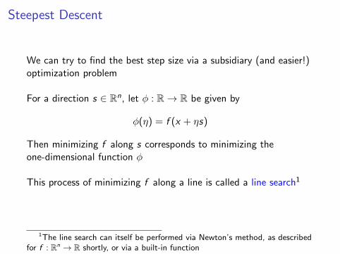
We can try to find the best step size via a subsidiary (and easier!)optimization problem
For a direction s ∈ Rn, let φ : R→ R be given by
φ(η) = f (x + ηs)
Then minimizing f along s corresponds to minimizing theone-dimensional function φ
This process of minimizing f along a line is called a line search1
1The line search can itself be performed via Newton’s method, as describedfor f : Rn → R shortly, or via a built-in function

Steepest Descent
Putting these pieces together leads to the steepest descent method:
1: choose initial guess x02: for k = 0, 1, 2, . . . do3: sk = −∇f (xk)4: choose ηk to minimize f (xk + ηksk)5: xk+1 = xk + ηksk6: end for
However, steepest descent often converges very slowly
Convergence rate is linear, and scaling factor can be arbitrarilyclose to 1
(Steepest descent will be covered on Assignment 5)

Newton’s Method
We can get faster convergence by using more information about f
Note that ∇f (x∗) = 0 is a system of nonlinear equations, hence wecan solve it with quadratic convergence via Newton’s method2
The Jacobian matrix of ∇f (x) is Hf (x) and hence Newton’smethod for unconstrained optimization is:
1: choose initial guess x02: for k = 0, 1, 2, . . . do3: solve Hf (xk)sk = −∇f (xk)4: xk+1 = xk + sk5: end for
2Note that in its simplest form this algorithm searches for stationary points,not necessarily minima

Newton’s Method
We can also interpret Newton’s method as seeking stationary pointbased on a sequence of local quadratic approximations
Recall that for small δ
f (x + δ) ≈ f (x) +∇f (x)T δ +1
2δTHf (x)δ ≡ q(δ)
where q(δ) is quadratic in δ (for a fixed x)
We find stationary point of q in the usual way:3
∇q(δ) = ∇f (x) + Hf (x)δ = 0
This leads to Hf (x)δ = −∇f (x), as in the previous slide
3Recall I.4 for differentiation of δTHf (x)δ

Newton’s Method
Python example: Newton’s method for minimization ofHimmelblau’s function
f (x , y) = (x2 + y − 11)2 + (x + y2 − 7)2
Local maximum of 181.617 at (−0.270845,−0.923039)
Four local minima, each of 0, at
(3, 2), (−2.805, 3.131), (−3.779,−3.283), (3.584,−1.841)

Newton’s Method
Python example: Newton’s method for minimization ofHimmelblau’s function
x
y
−8 −6 −4 −2 0 2 4 6 8−8
−6
−4
−2
0
2
4
6
8

Newton’s Method: Robustness
Newton’s method generally converges much faster than steepestdescent
However, Newton’s method can be unreliable far away from asolution
To improve robustness during early iterations it is common toperform a line search in the Newton-step-direction
Also line search can ensure we don’t approach a local max. as canhappen with raw Newton method
The line search modifies the Newton step size, hence often referredto as a damped Newton method
Newton’s Method: Robustness
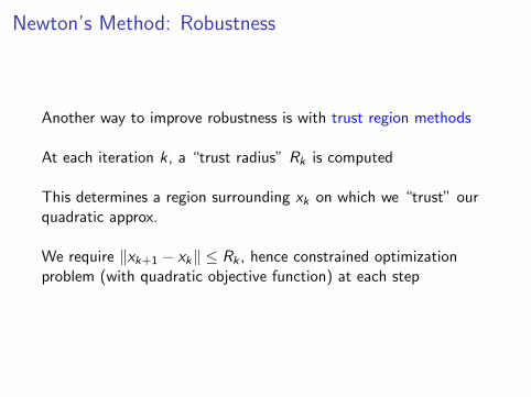
Another way to improve robustness is with trust region methods
At each iteration k , a “trust radius” Rk is computed
This determines a region surrounding xk on which we “trust” ourquadratic approx.
We require ‖xk+1 − xk‖ ≤ Rk , hence constrained optimizationproblem (with quadratic objective function) at each step

Newton’s Method: Robustness
Size of Rk+1 is based on comparing actual change,f (xk+1)− f (xk), to change predicted by the quadratic model
If quadratic model is accurate, we expand the trust radius,otherwise we contract it
When close to a minimum, Rk should be large enough to allow fullNewton steps =⇒ eventual quadratic convergence

Quasi-Newton Methods
Newton’s method is effective for optimization, but it can beunreliable, expensive, and complicated
I Unreliable: Only converges when sufficiently close to aminimum
I Expensive: The Hessian Hf is dense in general, hence veryexpensive if n is large
I Complicated: Can be impractical or laborious to derive theHessian
Hence there has been much interest in so-called quasi-Newtonmethods, which do not require the Hessian

Quasi-Newton Methods
General form of quasi-Newton methods:
xk+1 = xk − αkB−1k ∇f (xk)
where αk is a line search parameter and Bk is some approximationto the Hessian
Quasi-Newton methods generally lose quadratic convergence ofNewton’s method, but often superlinear convergence is achieved
We now consider some specific quasi-Newton methods

BFGS
The Broyden–Fletcher–Goldfarb–Shanno (BFGS) method is one ofthe most popular quasi-Newton methods:
1: choose initial guess x02: choose B0, initial Hessian guess, e.g. B0 = I3: for k = 0, 1, 2, . . . do4: solve Bksk = −∇f (xk)5: xk+1 = xk + sk6: yk = ∇f (xk+1)−∇f (xk)7: Bk+1 = Bk + ∆Bk
8: end for
where
∆Bk ≡yky
Tk
yTk sk−
BksksTk Bk
sTk Bksk

BFGS
See lecture: derivation of the Broyden root-finding algorithm
See lecture: derivation of the BFGS algorithm
Basic idea is that Bk accumulates second derivative information onsuccessive iterations, eventually approximates Hf well

BFGS
Actual implementation of BFGS: store and update inverse Hessianto avoid solving linear system:
1: choose initial guess x02: choose H0, initial inverse Hessian guess, e.g. H0 = I3: for k = 0, 1, 2, . . . do4: calculate sk = −Hk∇f (xk)5: xk+1 = xk + sk6: yk = ∇f (xk+1)−∇f (xk)7: Hk+1 = ∆Hk
8: end for
where
∆Hk ≡ (I − skρkyTk )Hk(I − ρkyksTk ) + ρksks
Tk , ρk =
1
yTk sk
BFGS
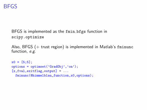
BFGS is implemented as the fmin bfgs function inscipy.optimize
Also, BFGS (+ trust region) is implemented in Matlab’s fminuncfunction, e.g.
x0 = [5;5];
options = optimset(’GradObj’,’on’);
[x,fval,exitflag,output] = ...
fminunc(@himmelblau_function,x0,options);

Conjugate Gradient Method
The conjugate gradient (CG) method is another alternative toNewton’s method that does not require the Hessian:
1: choose initial guess x02: g0 = ∇f (x0)3: x0 = −g04: for k = 0, 1, 2, . . . do5: choose ηk to minimize f (xk + ηksk)6: xk+1 = xk + ηksk7: gk+1 = ∇f (xk+1)8: βk+1 = (gT
k+1gk+1)/(gTk gk)
9: sk+1 = −gk+1 + βk+1sk10: end for

Constrained Optimization

Equality Constrained Optimization
We now consider equality constrained minimization:
minx∈Rn
f (x) subject to g(x) = 0,
where f : Rn → R and g : Rn → Rm
With the Lagrangian L(x , λ) = f (x) + λTg(x), we recall from thatnecessary condition for optimality is
∇L(x , λ) =
[∇f (x) + JTg (x)λ
g(x)
]= 0
Once again, this is a nonlinear system of equations that can besolved via Newton’s method

Sequential Quadratic Programming
To derive the Jacobian of this system, we write
∇L(x , λ) =
[∇f (x) +
∑mk=1 λk∇gk(x)
g(x)
]∈ Rn+m
Then we need to differentiate wrt to x ∈ Rn and λ ∈ Rm
For i = 1, . . . , n, we have
(∇L(x , λ))i =∂f (x)
∂xi+
m∑k=1
λk∂gk(x)
∂xi
Differentiating wrt xj , for i , j = 1, . . . , n, gives
∂
∂xj(∇L(x , λ))i =
∂2f (x)
∂xi∂xj+
m∑k=1
λk∂2gk(x)
∂xi∂xj

Sequential Quadratic Programming
Hence the top-left n × n block of the Jacobian of ∇L(x , λ) is
B(x , λ) ≡ Hf (x) +m∑
k=1
λkHgk (x) ∈ Rn×n
Differentiating (∇L(x , λ))i wrt λj , for i = 1, . . . , n, j = 1, . . . ,m,gives
∂
∂λj(∇L(x , λ))i =
∂gj(x)
∂xi
Hence the top-right n ×m block of the Jacobian of ∇L(x , λ) is
Jg (x)T ∈ Rn×m

Sequential Quadratic Programming
For i = n + 1, . . . , n + m, we have
(∇L(x , λ))i = gi (x)
Differentiating (∇L(x , λ))i wrt xj , for i = n + 1, . . . , n + m,j = 1, . . . , n, gives
∂
∂xj(∇L(x , λ))i =
∂gi (x)
∂xj
Hence the bottom-left m × n block of the Jacobian of ∇L(x , λ) is
Jg (x) ∈ Rm×n
. . . and the final m ×m bottom right block is just zero(differentiation of gi (x) w.r.t. λj)

Sequential Quadratic Programming
Hence, we have derived the following Jacobian matrix for∇L(x , λ): [
B(x , λ) JTg (x)Jg (x) 0
]∈ R(m+n)×(m+n)
Note the 2× 2 block structure of this matrix (matrices with thisstructure are often called KKT matrices4)
4Karush, Kuhn, Tucker: did seminal work on nonlinear optimization

Sequential Quadratic Programming
Therefore, Newton’s method for ∇L(x , λ) = 0 is:[B(xk , λk) JTg (xk)Jg (xk) 0
] [skδk
]= −
[∇f (xk) + JTg (xk)λk
g(xk)
]for k = 0, 1, 2, . . .
Here (sk , δk) ∈ Rn+m is the kth Newton step
Sequential Quadratic Programming
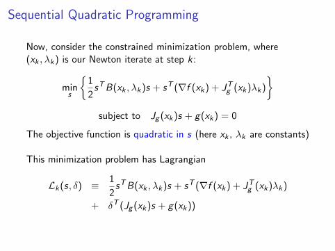
Now, consider the constrained minimization problem, where(xk , λk) is our Newton iterate at step k :
mins
{1
2sTB(xk , λk)s + sT (∇f (xk) + JTg (xk)λk)
}subject to Jg (xk)s + g(xk) = 0
The objective function is quadratic in s (here xk , λk are constants)
This minimization problem has Lagrangian
Lk(s, δ) ≡ 1
2sTB(xk , λk)s + sT (∇f (xk) + JTg (xk)λk)
+ δT (Jg (xk)s + g(xk))

Sequential Quadratic Programming
Then solving ∇Lk(s, δ) = 0 (i.e. first-order necessary conditions)gives a linear system, which is the same as the kth Newton step
Hence at each step of Newton’s method, we exactly solve aminimization problem (quadratic objective fn., linear constraints)
An optimization problem of this type is called a quadratic program
This motivates the name for applying Newton’s method toL(x , λ) = 0: Sequential Quadratic Programming (SQP)
Sequential Quadratic Programming
SQP is an important method, and there are many issues to beconsidered to obtain an efficient and reliable implementation:
I Efficient solution of the linear systems at each Newtoniteration — matrix block structure can be exploited
I Quasi-Newton approximations to the Hessian (as in theunconstrained case)
I Trust region, line search etc to improve robustness
I Treatment of constraints (equality and inequality) during theiterative process
I Selection of good starting guess for λ
Penalty Methods
Another computational strategy for constrained optimization is toemploy penalty methods
This converts a constrained problem into an unconstrained problem
Key idea: Introduce a new objective function which is a weightedsum of objective function and constraint

Penalty Methods
Given the minimization problem
minx
f (x) subject to g(x) = 0
we can consider the related unconstrained problem
minxφρ(x) = f (x) +
1
2ρg(x)Tg(x) (∗∗)
Let x∗ and x∗ρ denote the solution of (∗) and (∗∗), respectively
Under appropriate conditions, it can be shown that
limρ→∞
x∗ρ = x∗

Penalty Methods
In practice, we can solve the unconstrained problem for a largevalue of ρ to get a good approximation of x∗
Another strategy is to solve for a sequence of penalty parameters,ρk , where x∗ρk serves as a starting guess for x∗ρk+1
Note that the major drawback of penalty methods is that a largefactor ρ will increase the condition number of the Hessian Hφρ
On the other hand, penalty methods can be convenient, primarilydue to their simplicity

Linear Programming

Linear Programming
As we mentioned earlier, the optimization problem
minx∈Rn
f (x) subject to g(x) = 0 and h(x) ≤ 0, (∗)
with f , g , h affine, is called a linear program
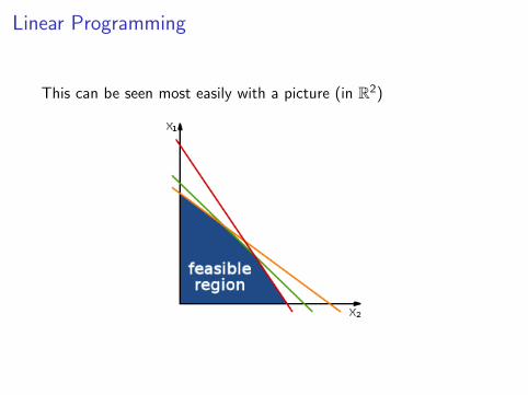
The feasible region is a convex polyhedron5
Since the objective function maps out a hyperplane, its globalminimum must occur at a vertex of the feasible region
5Polyhedron: a solid with flat sides, straight edges
Linear Programming
This can be seen most easily with a picture (in R2)

Linear Programming
The standard approach for solving linear programs is conceptuallysimple: examine a sequence of the vertices to find the minimum
This is called the simplex method
Despite its conceptual simplicity, it is non-trivial to develop anefficient implementation of this algorithm
We will not discuss the implementation details of the simplexmethod...

Linear Programming
In the worst case, the computational work required for the simplexmethod grows exponentially with the size of the problem
But this worst-case behavior is extremely rare; in practice simplexis very efficient (computational work typically grows linearly)
Newer methods, called interior point methods, have beendeveloped that are polynomial in the worst case
Nevertheless, simplex is still the standard approach since it is moreefficient than interior point for most problems

Linear Programming
Python example: Using cvxopt, solve the linear program
minx
f (x) = −5x1 − 4x2 − 6x3
subject to
x1 − x2 + x3 ≤ 20
3x1 + 2x2 + 4x3 ≤ 42
3x1 + 2x2 ≤ 30
and 0 ≤ x1, 0 ≤ x2, 0 ≤ x3
(LP solvers are efficient, main challenge is to formulate anoptimization problem as a linear program in the first place!)
PDE Constrained Optimization

PDE Constrained Optimization
We will now consider optimization based on a function thatdepends on the solution of a PDE
Let us denote a parameter dependent PDE as
PDE(u(p); p) = 0
I p ∈ Rn is a parameter vector; could encode, for example, theflow speed and direction in a convection–diffusion problem
I u(p) is the PDE solution for a given p
PDE Constrained Optimization
We then consider an output functional g ,6 which maps an arbitraryfunction v to R
And we introduce a parameter dependent output, G(p) ∈ R, whereG(p) ≡ g(u(p)) ∈ R, which we seek to minimize
At the end of the day, this gives a standard optimization problem:
minp∈RnG(p)
6A functional is just a map from a vector space to R

PDE Constrained Optimization
One could equivalently write this PDE-based optimization problemas
minp,u
g(u) subject to PDE(u; p) = 0
For this reason, this type of optimization problem is typicallyreferred to as PDE constrained optimization
I objective function g depends on u
I u and p are related by the PDE constraint
Based on this formulation, we could introduce Lagrange multipliersand proceed in the usual way for constrained optimization...

PDE Constrained Optimization
Here we will focus on the form we introduced first:
minp∈RnG(p)
Optimization methods usually need some derivative information,such as using finite differences to approximate ∇G(p)

PDE Constrained Optimization
But using finite differences can be expensive, especially if we havemany parameters:
∂G(p)
∂pi≈ G(p + hei )− G(p)
h,
hence we need n + 1 evaluations of G to approximate ∇G(p)!
We saw from the Himmelblau example that supplying the gradient∇G(p) cuts down on the number of function evaluations required
The extra function calls due to F.D. isn’t a big deal forHimmelblau’s function, each evaluation is very cheap
But in PDE constrained optimization, each p → G(p) requires afull PDE solve!

PDE Constrained Optimization
Hence for PDE constrained optimization with many parameters, itis important to be able to compute the gradient more efficiently
There are two main approaches:
I the direct method
I the adjoint method
The direct method is simpler, but the adjoint method is muchmore efficient if we have many parameters

PDE Output Derivatives
Consider the ODE BVP
−u′′(x ; p) + r(p)u(x ; p) = f (x), u(a) = u(b) = 0
which we will refer to as the primal equation
Here p ∈ Rn is the parameter vector, and r : Rn → R
We define an output functional based on an integral
g(v) ≡∫ b
aσ(x)u(x)dx ,
for some function σ; then G(p) ≡ g(u(p)) ∈ R

The Direct Method
We observe that
∂G(p)
∂pi=
∫ b
aσ(x)
∂u
∂pidx
hence if we can compute ∂u∂pi
, i = 1, 2, . . . , n, then we can obtainthe gradient
Assuming sufficient smoothness, we can “differentiate the ODEBVP” wrt pi to obtain,
− ∂u∂pi
′′(x ; p) + r(p)
∂u
∂pi(x ; p) = − ∂r
∂piu(x ; p)
for i = 1, 2, . . . , n

The Direct Method
Once we compute each ∂u∂pi
we can then evaluate ∇G(p) byevaluating a sequence of n integrals
However, this is not much better than using finite differences: Westill need to solve n separate ODE BVPs
(Though only the right-hand side changes, so could LU factorizethe system matrix once and back/forward sub. for each i)

Adjoint-Based Method
However, a more efficient approach when n is large is the adjointmethod
We introduce the adjoint equation:
−z ′′(x ; p) + r(p)z(x ; p) = σ(x), z(a) = z(b) = 0

Adjoint-Based Method
Now,
∂G(p)
∂pi=
∫ b
aσ(x)
∂u
∂pidx
=
∫ b
a
[−z ′′(x ; p) + r(p)z(x ; p)
] ∂u∂pi
dx
=
∫ b
az(x ; p)
[− ∂u∂pi
′′(x ; p) + r(p)
∂u
∂pi(x ; p)
]dx ,
where the last line follows by integrating by parts twice (boundaryterms vanish because ∂u
∂piand z are zero at a and b)
(The adjoint equation is defined based on this “integration byparts” relationship to the primal equation)
Adjoint-Based Method
Also, recalling the derivative of the primal problem with respect topi :
− ∂u∂pi
′′(x ; p) + r(p)
∂u
∂pi(x ; p) = − ∂r
∂piu(x ; p),
we get∂G(p)
∂pi= − ∂r
∂pi
∫ b
az(x ; p)u(x ; p)dx
Therefore, we only need to solve two differential equations (primaland adjoint) to obtain ∇G(p)!
For more complicated PDEs the adjoint formulation is morecomplicated but the basic ideas stay the same