NBS

PUBLICATIONS

AlllDE 7Dbb3b

»^ffMi«»IIr,^3..

NBS TECHNICAL NOTE 1311

U.S. DEPARTMENT OF COMMERCE / National Bureau of Standards

TM he National Bureau of Standards* was established by an act of Congress on March 3, 1901. The Bureau's overall

J^^ goal is to strengthen and advance the nation's science and technology and facilitate their effective appUcation for

public benefit. To this end, the Bureau conducts research to assure international competitiveness and leadership of U.S.industry, science arid technology. NBS work involves development and transfer of measurements, standards and related

science and technology, in support of continually improving U.S. productivity, product quality and reliability, innovation

and underlying science and engineering. The Bureau's teclmical work is performed by the National MeasurementLaboratory, the National Engineering Laboratory, the Institute for Computer Sciences and Technology, and the Institute

for Materials Science and Engineering.

The National Measurement Laboratory

Provides the national system of physical and chemical measurement;coordinates the system with measurement systems of other nations andfurnishes essential services leading to accurate and uniform physical andchemical measurement throughout the Nation's scientific community,industry, and commerce; provides advisory and research services to other

Government agencies; conducts physical and chemical research; develops,

produces, and distributes Standard Reference Materials; provides

calibration services; and manages the National Standard Reference DataSystem. The Laboratory consists of the following centers:

• Basic Standards^• Radiation Research• Chemical Physics• Analytical Chemistry

The National Engineering Laboratory

Provides technology and technical services to the public and private sectors

to address national needs and to- solve national problems; conducts research

in engineering and applied science in support of these efforts; buUds andmaintains competence in the necessary disciplines required to carry out this

research and technical service; develops engineering data and measurementcapabilities; provides engineering measurement traceability services;

develops test methods and proposes engineering standards and codechanges; develops and proposes new engineering practices; and develops

and improves mechanisms to transfer results of its research to the ultimate

user. TTie Laboratory consists of the following centers:

• AppUed Mathematics• Electronics and Electrical

Engineering^• Manufacturing Engineering• Building Technology• Fire Research• Chemical Engineering^

The Institute for Computer Sciences and Technology

Conducts research and provides scientific and technical services to aid

Federal agencies in the selection, acquisition, appUcation, and use ofcomputer technology to improve effectiveness and economy in Govenmientoperations in accordance with Pubhc Law 89-306 (40 U.S.C. 759),

relevant Executive Orders, and other directives; carries out this mission bymanaging the Federal Information Processing Standards Program,developing Federal ADP standards guidelines, and managing Federal

participation in ADP voluntary standardization activities; provides scientific

and technological advisory services and assistance to Federal agencies; andprovides the technical foundation for computer-related policies of the

Federal Govenunent. The Institute consists of the following divisions:

Information Systems Engineering

Systems and Software

TechnologyComputer Security

Systems and NetworkArchitecture

Advanced Computer Systems

The Institute for Materials Science and Engineering

Conducts research and provides measurements, data, standards, reference

materials, quantitative understanding and other technical informationfundamental to the processing, structure, properties and performance ofmaterials; addresses the scientific basis for new advanced materials

technologies; plans research around cross-cutting scientific themes such as

nondestructive evaluation and phase diagram development; overseesBureau-wide technical programs in nuclear reactor radiation research andnondestructive evaluation; and broadly disseminates generic technicalinformation resulting fi-om its programs. The Institute consists of thefollowing Divisions:

• Ceramics• Fracture and Deformation^• Polymers• Metallurgy• Reactor Radiation

'Headquarters and Laboratories at Gaithersburg, MD, unless otherwise noted; mailing addressGaithersburg, MD 20899.

^Some divisions within the center are located at Boulder, CO 80303.'Located at Boulder, CO, with some elements at Gaithersburg, MD

Research Information Center

National bureau of Standards

Gaithersburg, Maryiaaid 20899

Extrapolation Range Measurements for

Determining Antenna Gain and Polarization

Andrew G. Repjar

Allen C. Newell

Douglas T. Tamura

Electromagnetic Fields Division

Center for Electronics and Electrical Engineering

National Engineering Laboratory

National Bureau of StandardsBoulder, Colorado 80303-3328

0^

ML %

*'"'Eau o«

U.S. DEPARTMENT OF COMMERCE, Clarence J. Brown, Acting Secretary

NATIONAL BUREAU OF STANDARDS, Ernest Ambler, Director

Issued August 1987

National Bureau of Standards Technical Note 1311

Natl. Bur. Stand. (U.S.), Tech Note 1311, 88 pages (Aug. 1987)

CODEN:NBTNAE

U.S. GOVERNMENT PRINTING OFFICEWASHINGTON: 1987

For sale by the Superintendent of Documents, U.S. Government Printing Office, Washington, DC 20402

Contents

Page

1. Introduction 1

2. Definitions and Basic Concepts from a MeasurementPoint of View 3

2.1 Antenna Scattering Matrix Parameters 3

2.2 Generalization of the Three-Antenna MeasurementTechnique 8

2.3 Measurement Methods for the Extrapolation Technique 14

2.4 Description of Measurement System 15

3. Measurement Procedures 223.1 Alignment of Antennas 223.2 Receiver Calibration and Determination of ag 23

3.3 Amplitude, Phase and Distance Data, General 273.4 Amplitude Measurements 273.5 Phase Measurements 31

4. Numerical Techniques for Antenna Gain and PolarizationMeasurements 32

5. Error Analysi s 365.1 Propagation of Errors to Gain and Polarization

Parameters 385.2 Three Nominally Linearly Polarized Antennas 395.3 Two Nominally Linearly and One Nominally Circularly

Polarized Antenna Combination 406. Measurement Examples 42

6.1 X-Band Standard Gain Horns 426.2 V-Band Reflector Antennas 43

7. Improved Polarization Measurements 448. Swept Frequency Measurement Techniques 50

9. Summary 67

10. References 68Appendix A. Extension of Extrapolation Technique to Correct

for Effects of Ground Reflections A-1Introduction , A-2Discussion of Measurement Procedure A-2Extrapolation Method A-2Analysis A-3Resul ts A-4Concl usions A-4References A-5

Appendix 3. Standard NBS Calibration Report B-1

m

List of Figures

Figure Page

1 Waveguide two-port junction 4

2 Plane-wave scattering-matrix description of an antenna 5

3 Schematic of two antennas oriented for measurement 10

4 Extrapolation range 16

5 Precision rail alignment 17

6 Antenna alignment 197 Fixed frequency measurements 218 Steps in making a strain relief loop to minimize cable

movement at connector joints 269 Extrapolation data for two X-band standard gain horns 28

10 Extrapolation data showing multipath interference andaveraged curve for two 45 cm (18 in), millimeter-wave,parabol i c-reflector antennas 29

11 Averaged extrapolation data for the same antenna as

in figure 8 2912 Measured phase difference between bk and bg plotted as a

function of distance for a 1.2 m (4 ft) diameter

parabolic antenna at 8 GHz 33

13 Measured-data, two-term polynomial fit, and residuals forX-band conical horn (gain « 22 dB) 35

14 Measured-data, five-term polynomial fit, and residuals forX-band conical horn (gain « 22 dB) 37

15 Polarization measurements 46

16 Swept frequency measurements 51

17 Swept frequency, reflection coefficient measurement(amplitude) for generator port 52

18 Swept frequency, reflection coefficient measurement(phase) for generator port 53

19 Swept frequency, reflection coefficient measurement(amplitude) for a long pyramidal horn 54

20 Swept frequency, reflection coefficient measurement(phase) for a long pyramidal horn 55

21 Mismatch correction calculated from measuredreflect ion -coefficient data 56

22 Near-zone correction obtained from extrapolationmethod for fixed-frequency measurements at 11.7, 14.5,15.0, 17.0, and 18.1 GHz 58

23 Swept frequency amplitude measurement with antennasin place at fixed distance of about a^/x 59

24 Swept frequency reference amplitude curve obtained withgenerator and load ports connected directly together 60

25 Insertion loss including mismatch and near-zone correc-tions. This is the difference between the referencecurve and amplitude curve with antennas in place. Thehigh-frequency oscillations are due to multiple reflec-tions between the antennas 61

26 Insertion loss with multiple reflections averaged out 62

27 Average gain for a pair of antennas 63

28 Final gain values for a long Ku-band horn. The oscil-lations about the nominal values are approximately±0.04 dB and are due to mismatches at the throat andaperture of the horn 64

29 Final gain values for a standard gain horn. The oscil-lations about the nominal values are approximately+0.1 dB and are due to mismatches at the throat andaperture of the horn 65

30 Comparison between theoretical gain and gain measured bythe swept frequency technique for an X-band pyramidalhorn. Gain values indicated by the * were obtained bythe extrapol ati on method 66

List of Tables

Table Page

1 Data and errors for X-band antennas 432 Data and errors for mn-wave antennas 443 Results of polarization measurements 49

vi

Extrapolation Range Measurements for Determining AntennaGain and Polarization

Andrew G. Repjar, Allen C. Newell, and Douglas T. Tamura

National Bureau of StandardsElectromagnetic Fields Division

Boulder Colorado 80303

The extrapolation range measurement technique for determiningthe power gain and polarization of antennas at reduced range dis-tances is described. It is based on a generalized three-antennaapproach and does not require quantitative a priori knowledge ofthe antennas. During the past decade, it has been extensivelyused by the National Bureau of Standards, Boulder, Colorado, tocalibrate antenna gain standards for industry and other agencieswithin ±0.1 dB. To help one understand how calibrations of thisaccuracy are achieved, the extrapolation range description in-

cludes discussions on the required theory, the measurement pro-cedures, the range configuration and instrumentation, the errors,and some measurement examples. Recent extensions of the extrapo-lation method required for swept/stepped frequency gain calibra-tions and for corrections to reduce ground reflection effects, arealso presented.

Key words: antenna calibrations; antenna measurements; antennaranges; antennas; near-field measurements; probe antennas; stan-dard gain horns; swept frequency measurements

1. Introduction

Accurate antenna gain standards are necessary to evaluate and verify the

performance of communication, radar, navigation, remote sensing, and other

systems that transmit or receive radiated electromagnetic energy. Until the

mid-1970s, the most common method of measuring the antenna gain and polariza-

tion for these systems was a substitution technique, where the response of the

test antenna to an incident plane-wave field was compared with that of one or

more standard antennas. Since then, near-field measurement techniques, where

a probe scans over a planar [1], cylindrical [2,3], and spherical [4,5] sur-

face, have been extensively used. In either case, the characteristics of the

standard antennas or probe must be determined.

Computed gain and polarization values for a standard antenna do not pro-

vide a satisfactory solution for high accuracy measurements. The gain of

pyramidal horn antennas, used extensively as standards or probes [6,7] may be

calculated within an estimated uncertainty of about ±0.3 dB. Similarly, gain

calculations for both smooth and corrugated conical horns [8,9] have about the

same accuracy. The uncertainties in these calculated values are due to theo-

retical approximations and imperfect fabrication, problems not easily over-

come. For this reason, the National Bureau of Standards (NBS) has opted to

develop and employ "standard measurement methods" rather than "standard anten-

nas." By these methods, an arbitrary antenna can be accurately calibrated for

use as a gain and polarization transfer standard.

The well known, far-field three-antenna method is not suitable for accu-

rate absolute measurements of many standard antennas for several reasons. With

conventional far-field antenna ranges, the plane-wave condition is approxi-

mated by using large separation distances between the transmitting and receiv-

ing sites. However, for high gain antennas, ranges of sufficient length may

not be available. This is especially true when high accuracy is desired. For

example, to reduce the proximity correction of typical standard gain horns to

less than 0.05 dB requires a distance of about 32 (not 2) a^/x [10], where a

is the largest aperture dimension and x is the free-space wavelength. At such

large distances the errors due to ground reflections and scattering from other

objects can be significant. Additional errors can occur if the test and stan-

dard antennas have significantly different gains, patterns, or polarization

characteristics. Interference from other signals, and (at millimeter-wave

frequencies) strong atmospheric attenuation are other problems. To overcome

these difficulties and provide a means of accurately characterizing antenna

standards, NBS developed a new method, known as the extrapolation technique,

for evaluating directive antennas. This method is not well suited for pattern

measurements (although pattern data can be obtained), but it is the most accu-

rate method known for determining absolute gain and polarization. (Gain is

routinely obtained within 0.1 dB.) Hence, it is most useful in evaluating

standards and for measuring antennas when the highest accuracy is required.

The theoretical basis was developed by Wacker [11], and its application to

accurate antenna measurements has been described briefly by Newell and Kerns

[12] and more fully in an experimentally oriented paper by Newell et al . [13].

The method uses a generalized three-antenna approach which does not require

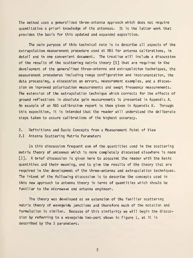
quantitative a priori knowledge of the antennas. It is the latter work that

provides the basis for this updated and expanded exposition.

The main purpose of this technical note is to describe all aspects of the

extrapolation measurement procedure used at NBS for antenna calibrations, in

detail and in one convenient document. The treatise will include a discussion

of the results of the scattering matrix theory [1] that are required in the

development of the generalized three-antenna and extrapolation techniques, the

measurement procedures including range configuration and instrumentation, the

data processing, a discussion on errors, measurement examples, and a discus-

sion on improved polarization measurements and swept frequency measurements.

The extension of the extrapolation technique which corrects for the effects of

ground reflections in absolute gain measurements is presented in Appendix A.

An example of an NBS calibration report is then given in Appendix B. Through

this exposition, it is intended that the reader will understand the deliberate

steps taken to assure calibrations of the highest accuracy.

2. Definitions and Basic Concepts from a Measurement Point of View

2.1 Antenna Scattering Matrix Parameters

In this discussion frequent use of the quantities used in the scattering

matrix theory of antennas which is more completely discussed elsewhere is made

[1]. A brief discussion is given here to acquaint the reader with the basic

quantities and their meaning, and to give the results of the theory that are

required in the development of the three-antenna and extrapolation techniques.

The intent of the following discussion is to describe the concepts used in

this new approach to antenna theory in terms of quantities which should be

familiar to the microwave and antenna engineer.

The theory was developed as an extension of the familiar scattering

matrix theory of waveguide Junctions and therefore much of the notation and

formulation is similar. Because of this similarity we will begin the discus-

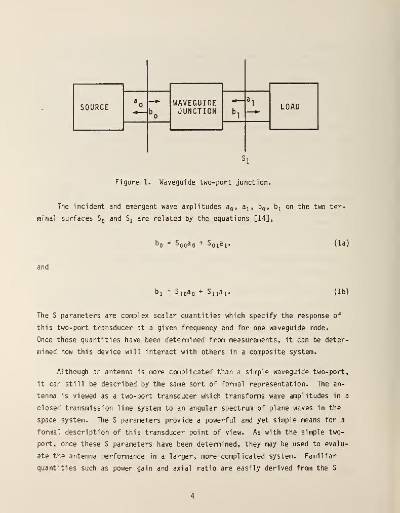
sion by referring to a waveguide two-port shown in figure 1, as it is .

described by the S parameters.

SOURCEWAVEGUIDEJUNCTION

LOAD^ ^

"i

^1

Figure 1. Waveguide two-port junction.

The incident and emergent wave amplitudes ag, a^, bg, b^ on the two ter-

minal surfaces Sq and S^ are related by the equations [14],

^0 " Sqo^O '' Sqi^Ij (la)

and

b, = S 10^0 + S 11^1' (lb)

The S parameters are complex scalar quantities which specify the response of

this two-port transducer at a given frequency and for one waveguide mode.

Once these quantities have been determined from measurements, it can be deter-

mined how this device will interact with others in a composite system.

Although an antenna is more complicated than a simple waveguide two-port,

it can still be described by the same sort of formal representation. The an-

tenna is viewed as a two-port transducer which transforms wave amplitudes in a

closed transmission line system to an angular spectrum of plane waves in the

space system. The S parameters provide a powerful and yet simple means for a

formal description of this transducer point of view. As with the simple two-

port, once these S parameters have been determined, they may be used to evalu-

ate the antenna performance in a larger, more complicated system. Familiar

quantities such as power gain and axial ratio are easily derived from the S

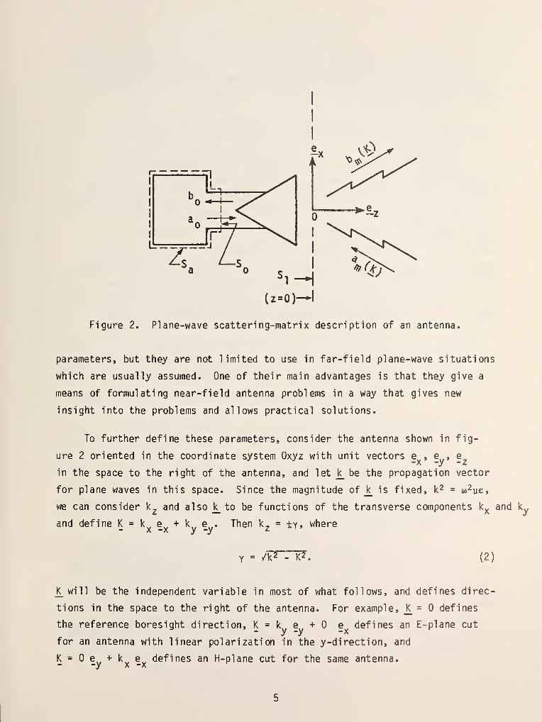
Figure 2. Plane-wave scattering-matrix description of an antenna.

parameters, but they are not limited to use in far-field plane-wave situations

which are usually assumed. One of their main advantages is that they give a

means of formulating near-field antenna problems in a way that gives new

insight into the problems and allows practical solutions.

To further define these parameters, consider the antenna shown in fig-

ure 2 oriented in the coordinate system Oxyz with unit vectors e , e , e-X -y - z

in the space to the right of the antenna, and let k_ be the propagation vector

for plane waves in this space. Since the magnitude of _k_ is fixed, k^ = w^pe,

we can consider k^ and also k_ to be functions of the transverse components k^ and ky

and define K = k e + k e ,

X -X y -yThen k^ = +y, where

Y = /k2 - K2. (2)

K_will be the independent variable in most of what follows, and defines direc-

tions in the space to the right of the antenna. For example, J<= defines

the reference boresight direction, K = k e +0 e defines an E-plane cuta ' - y -y -X ^

for an antenna with linear polarization in the y-di recti on, and

K = e + k e defines an H-plane cut for the same antenna.— —y X —X

In addition to the unit vectors in the x, y, and z directions, we define

two additional vectors in the x-y plane which are used in the formulation.

These vectors, <i and <2 are

5i ^ y\^\ !52"^ §7 X !5i* (3)

In figure 2, ag and bg are incident and emergent wave amplitudes at the

surface Sq just as in the waveguide junction formulation, a^i^—^ ^^^ '^m^A) ^^^

spectral density functions for incoming and outgoing plane waves and are anal-

ogous to ag and bg. This decomposition of the transverse electric field into

a continuous angular spectrum of plane waves is analogous to the familiar

practice of analyzing a complicated time function in terms of its frequency

components. Indeed, there are many concepts from time and frequency domain

analysis which can be carried over to the antenna problem and give new insight

to the processes involved. These ideas are formalized by the following equa-

tions [15] which define the S-parameter functions that characterize the

antenna:

2

bo = Sggag + / I Soi(m,K) a (K) dK, (4a)m-1 - mm=l

and

2

b (K) = Sio(m,K) ag + / I Sii(m,K;n,L) a (L) dL, (4b)m - - ^^^ . . n - -

where the summation is over two values of the polarization index m or n, (cor-

responding to the tv/o orthogonal polarizations, k^ and <2 of the wave in the

x-y plane), integration is over all values of K (or L), and dK denotes the

surface element for integration (e.g., dk^dk ).

The significance of each parameter can best be seen by considering two

special cases. First assume that the antenna is transmitting into free space

and therefore there are no waves incident from the right, a^(_K) = 0. We then

have

bo = Sogag (5a)

and

bn,(!<) = Sio(m,K) ao. (5b)

Sqo is thus a simple Input reflection coefficient term. Sio(m»K) defines the

transmitting characteristic since it describes how input wave amplitude ag is

transformed by the antenna into an angular pattern of plane waves bj^(J<_).

Next assume that the antenna is being used as a receiver with a matched

load termination and therefore ag = 0. We now have

2

bo = / I Soi(m,K) a (K) dK, (6a)m=l

and

2

b (K) = / I Sii(m,K;n,L) a (L) dL. (6b)m -

^^^. - n - -

Soi(f"»'^) is called the receiving characteristic since it describes how the

antenna responds to an incident spectrum of plane waves ci^(J<)» Sii(m,K;n,L)

is called the scattering characteristic as it describes how waves incident

from the right dire scattered back into the same space.

If the antenna is reciprocal, Sio(fn»K) and Soi(m,K) are related by the

reciprocity relation,

- no Soi(m,l<) = n^(l<) Sio(m, - K), (7)

1/2where m = we/y, n2 = Y/(wy) and no = (eq/uo) » is the characteristic admit-

tance of free space.

If we define the vectorial transmission spectrum as

Sio(K) = Sio(l,K) <! + Sio(2,!<) ^2, (8)

then the transverse electric field at large distances r from the source is

given by [15]

§t(r)= -^T^ cose Sio(R k/r) ao e'^\ (9)

where _r is the position vector with transverse part _R, r = |r|, and e is the

angle between k_ and ^, or equivalently the polar angle of r_ relative to the

z-axis. The power gain function is also given in terms of Sio(K) 3S

47rk2 cose [|Sjo(l,K)|2 m + |Sjo(2,K)|2 nj^'^>

.o(l"- ISooh'-

• '^°'

Since the electric field, the receiving characteristic for a reciprocal

antenna, and the gain function can all be found from Sio(K), the measurement

objective is then to determine Siq(K), or its value in certain important

directions such as the on-axis value Sio(0)»

2.2 Generalization of the Three-Antenna Measurement Technique

A three-antenna measurement to determine the gain of three antennas has

been available for some time [16]. This involves measuring the ratio of the

power input to the transmitting antenna to the available power from the re-

ceiving antenna and the separation distance between the antennas for the three

combination pairs. The three resulting equations may then be solved for the

gain of each antenna.

This approach implicitly assumes that far-field, plane-wave conditions

exist and that the three antennas have either known or identical polarization

characteristics.

Since only power ratios are measured in the above technique, no informa-

tion is obtained about the polarization states of the three antennas. Various

other methods have been used to measure antenna polarization [17], but they

all involve the use of at least one antenna whose polarization is assumed to

be known.

The generalized three-antenna method [12] to be described here does not

require a quantitative knowledge of the polarization of any of the antennas.

It is sufficient to know that two are approximately linearly polarized and the

polarization of the third is either linear or circular with an approximate

direction of polarization. With this knowledge and the measurement of the

appropriate quantities, both the gain and polarization of one or more of the

antennas can be determined.

Kerns [1] derives the coupling equations for the general situation when

only one of the three antennas is reciprocal. For simplicity, and because it

is the usual case, we will assume that the two antennas which are used in the

receiving mode are reciprocal.

Now suppose that we have two antennas whose transmission characteristics1 2

are given by Sio(K) and Sio(K) when each antenna is placed in a specific

orientation in the reference coordinate system. The prescribed orientation is

such that the antenna coordinate system is coincident with the reference sys-

tem. The antenna coordinate system is defined with its z-axis in the electri-

cal boresight direction, and the x- and y-axes defined by reference lines

scribed on or otherwise defined on the antenna structure. The placement of

these fiducial marks on the antenna is essentially arbitrary, but once chosen

they fix the axes of the antenna and therefore the coordinate system used to

define Sio(K). In practice, it simplifies and improves the accuracy of the

measurement to place the reference lines so that one axis is approximately

parallel to the principal component of the electric field. The y-axis will be

so chosen in the following.

With these choices of references axes, let antenna number 1 be placed in

the prescribed orientation in the reference coordinate system and used as the

transmitting antenna. Let the other antenna be placed in a receiving orienta-

tion by a 180 deg rotation in the reference coordinate system about the y-axis

and a translation along the z-axis to z = d. The two antennas are shown sche-

matically in figure 3 with appropriate terminal surfaces and wave amplitudes

shown.

In the following development, the transmission charateristic Sio(K) will

be used, but since the objective is to determine gain and polarization in the

boresight direction, we need only the on-axis value, Sio{0)» A simplified

notation may therefore be adopted which will eliminate the double subscript

and the explicit reference to K = 0. Both linear and circular components of

TRANSMITTINGSYSTEM

(z = 0)

-e,

(z=d)

K

RECEIVINGSYSTEM

Figure 3. Schematic of two antennas oriented for measurement.

Siq(0) will be required, and these are defined as follows. Let _e^ and

_ey be unit basis vectors in the x and y directions and define [18]

(11a)

f = (e^ - i e^)//?. (lib)

Then

Ep = e exp[i(kz-a)t)] (12a)

and

E. = e" exp[i(kz-a)t)] (12b)

are respectively right and left circularly polarized plane waves traveling in

the +z directions. The time dependence here is exp(-ia)t), and the definitions

of polarization used here are in agreement with the IEEE Standard No. 149

(Test Procedure for Antennas, 1979), and correspond to the definitions of

right- and left-handed screw threads.

10

The linear and circular components of Siq(0), using the simplified nota-

tion, will be referred to as X, Y, R and L such that Sio(O) = X e + Y e+ _

- -X -y= Re + Le , and the transformation equations are

R = (X - iY)//?, L = (X + iY)//7,

X = (R + L)//7, Y = i(R - L)//?.

(13a)

(13b)

The on-axis components for the three antennas will be distinguished by a

single subscript, ^iox^°^ " ^1' Hoy^^^ " ^2' etc.

In the bores ight direction, the gain and polarization quantities are

given by

Gain = G =-4Trk2(|x|^- +

(1 '00

Yj2) _ 4Trk2(|L|2 +

•) (1 '00

R|2)

Linear Polarization Ratio = p« = y*

Circular Polarization Ratio = p^ =-5,C K

Axial Ratio = A =R + L

R - Land

Tilt Angle = t = I/2 arg (p^).

(14)

(15)

(16)

(17)

(18)

With antennas 1 and 2 in their initial orientation as previously described and

shown in figure 3, the coupling equation is [1,13,15]

X1X2 - Y1Y2 - ^^ (

lim .^it-"^ (1 - V2) ^-ikd

l-H» 2iTik) -= DI2. (19)

where V2 is the reflection coefficient for antenna number 2, and r is the

reflection coefficient for the load.

Now let the receiving antenna be further reoriented by rotating it about

the z-axis by 90 deg in the direction from x to y. The coupling equation for

this orientation is

11

X Y . X Y- ^- bad)d (1 - r^r,) e-'^' _

X1Y2 + X2Y1 j^ [-

27rk J = ^12.

where bo(d) denotes the output wave amplitude for the second orientation.

Equations similar to (19) and (20) may be written for the other two

antenna pair combinations which yields six equations in six unknown quanti-

ties. These six equations may be expressed by the two general equations for

transmission from antenna m to antenna n as

XX - Y Y = D' , (21a)n m n m nm ^ '

X Y + X Y = D" . (21b)n m m n nm ^ '

These coupling equations have a very simple form and yet contain a great deal

of information about the antenna interaction. Since they are written in terms

of complex vector components, they take into account the vector character of

the field and the receiving antennas response to that vector field. This is

in contrast to the Friis transmission equation which relates only the scalar

quantities of power and gain and includes no information about the vector

nature of the transfer functions. It is possible to write equations using

gain, axial ratio, and tilt angle to relate transmitted and received power

[18], but such expressions are much more complex and yet contain no more

information than eq (21).

To solve the resulting set of six equations we define

A = (D' - iD" 1/2, (22a)nm '^ nm nm^' ^

and

T = (D' + iD" 1/2, (22b)^ nm ^ nm nm^ ^

and note that eq (21) can be written as

RR=A, LL = y . (23)n m nm' n m ^ nm ^

'

12

The solution for circular and linear components now follows and gives, for

example.

,-.; A21A13

^32

V^21^13

^32

(24a)

(24b)

and

= ±-li J~^ll^± J ^21^1

^ ' /2 \ ^32"^ ^32Xi=±-^ \—Z--± \-T-- (25a)

^ ' /2 \ ^32 "" ^ ^32Yi =±-Z \-7— ^ \-F— • (25b)

In these equations the signs are correlated vertically but not horizontally.

If the upper signs are used in one of the equations, they must be used in the

other two also. A qualitative knowledge of|p |, either from a priori informa-

tion or the measured data, is required to indicate the proper choice. One

choice will yield |p |> 1 while the other choice gives |p |

< 1, and the pro-

per choice will yield results consistent with |p»|«

Difficulties can arise in the solution of eq (24) if one or more of the

antennas is nearly circularly polarized. For example, A32 may be nearly zero

if antenna 3 has nearly left-circular polarization. The two practical antenna

combinations are therefore either three linearly polarized antennas or two

linearly and one circularly polarized antenna. In the first case the gains

and polarizations are determined for all three, while in the latter the char-

acteristics of only the circular antenna will be completely determined.

If, however, three circularly polarized antennas are nominally polariza-

tion matched, then we can determine the principal components from either

eq (24a) or (24b). The circular polarizations can then be determined by an

improved polarization measurement technique which is discussed in detail in

Section 7. Similarly, if three linearly polarized antennas are nominally

polarization matched, then we can determine the principal components from

13

either eq (25a) or (25b). Then, the linear polarizations can also be deter-

mined using the improved polarization measurement technique. Although in

practice, these improved procedures are generally the rule, it is necessary to

understand thoroughly the above notations and development to facilitate the

comprehension of later sections.

2.3 Measurement Methods for the Extrapolation Technique

The data required to determine the D^j^'s are the ratio of output to input

signals for the two antenna orientations, |bo(d)/ao| and |bo(d)/ao|, and the

phase change resulting from the second antenna rotation, arg (bo(d)/bo(d)}.

This information, plus the separation distance d, the frequency f, and the

necessary reflection coefficients determine the D^^'s; the transmission compo-

nents can then be found from eqs (19) through (25). In principle the required

data could be obtained by well known far-field measurement methods, but the

extrapolation measurement approach will be described here because it has defi-

nite advantages for accurate absolute gain and polarization measurements.

The theory of the extrapolation technique was developed by Wacker [11],

and the main result is that for any two essentially arbitrary antennas the

received signal as a function of separation distance can be accurately repre-

sented by the power series

^o(d)=r^ I''P^'%11 ''^

I V (26)^ ^n^£ p=0 (d)'^P^^ q=0 d^

The significance of each term and subseries may be seen more clearly if a few

terms are written out explicitly to give

^0 p""^^ ^01 ^02 ^03

n i (27)

+

3ikd Aj^ Aj2 5ikd

The first series represents the direct transmission signal including near-zone

terms, the second series the first-order multiple reflection between the two

14

antennas, and the third series the higher order multiple reflections. Equa-

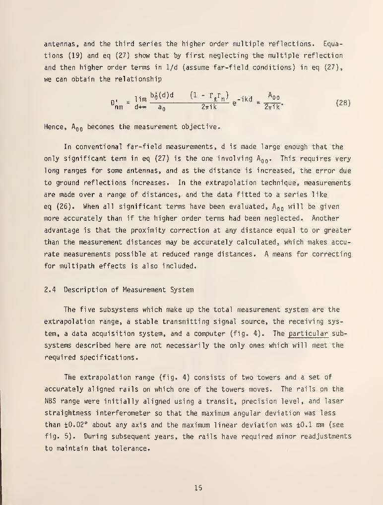
tions (19) and eq (27) show that by first neglecting the multiple reflection

and then higher order terms in 1/d (assume far-field conditions) in eq (27),

we can obtain the relationship

'^nm d-^" ao 2Trik ^ 27rik*^^^'

Hence, Aqq becomes the measurement objective.

In conventional far-field measurements, d is made large enough that the

only significant term in eq (27) is the one involving Aqq. This requires wery

long ranges for some antennas, and as the distance is increased, the error due

to ground reflections increases. In the extrapolation technique, measurements

are made over a range of distances, and the data fitted to a series like

eq (26). When all significant terms have been evaluated, Aqq will be given

more accurately than if the higher order terms had been neglected. Another

advantage is that the proximity correction at any distance equal to or greater

than the measurement distances may be accurately calculated, which makes accu-

rate measurements possible at reduced range distances. A means for correcting

for multipath effects is also included.

2.4 Description of Measurement System

The five subsystems which make up the total measurement system are the

extrapolation range, a stable transmitting signal source, the receiving sys-

tem, a data acquisition system, and a computer (fig. 4). The particular sub-

systems described here are not necessarily the only ones which will meet the

required specifications.

The extrapolation range (fig. 4) consists of two towers and a set of

accurately aligned rails on which one of the towers moves. The rails on the

NBS range were initially aligned using a transit, precision level, and laser

straightness interferometer so that the maximum angular deviation was less

than ±0.02° about any axis and the maximum linear deviation was ±0.1 mn (see

fig. 5). During subsequent years, the rails have required minor readjustments

to maintain that tolerance.

15

oo.<flC

Xtu

f'

—

r*

^ 1 1

ID.o E cc

LU

lisu:cr0:2 Ji t;

i^OCO T^-1 . ^f-

K* o' " ' Lj UJ

_ju.P j

t'Vl|E||jy|ji|t||lAi^AikAi UJ

VrrmrftVWW ccV?f|ljTff f T f f f f

1-liil^-/2 fiW ,

w If ,^ Hz / v ^*jj Z< / \ ^5 3cr / \ -J

<^ o ^H 2

^^ COcc o

UJ

iccUJ>UJoUJcc

00 Ui

OUJ2^

UI

<oc

zCOl_cotUJZ

5z ^ _l< CO

03Oor^S ^^ . I Q.

^4 OCoc ''h. Q.

\t o ^ CO13 ^^

>«A CD<

i<CC

zUi> \ / * o

CO

UJ 1 / ^5 oo A A 11 A ^5 UJUJ A A |A A ^^5 cccc PsM;^

im ,

0-

coAAMm^jajli

K-;-^;;*...;*.;.^^ ; ;^.;.tK;.;^:^^y^m ,

i . _ •-

II1 < W^z UJ 0<s^O t

^NTENN/J

lARIZATK AND LIGNMENMOUNT

LASER

FODISTA

MEASURI

O < 1

^1

^ '

oCDEftJ

J_

O

oQ.fOS-4->

X

Ll-

16

u

o

<czo

oUJcc

»->

ccuE

5-

OJ-

S-

•r—

u_

17

The moving tower is supported by roller bearings so that the tower can be

moved over the distance of the range as accurately as the rails are aligned. A

variable speed drive system is used to move the cart uniformly during the ex-

trapolation measurement. Plus and minus z movement must be smooth. The vari-

able speed is used primarily so that approximately 10 to 20 data points per

wavelength are taken over a range where the insertion loss changes from to

-20 dB. Thus, the time for the tower's z-axis movement varies depending on the

frequency and the total distance covered.

The separation distance, which must be measured to an accuracy of about 0.1

percent over the total range, can be determined by measuring the voltage across

a precision multiturn potentiometer whose rotation angle is proportional to the

separation distance between the towers. The important requirement is that the

readout be a linear function of distance. The present system uses a laser meas-

urement system which accurately measures the distance over the 10 m range.

Although data are not usually recorded over the complete range, the towers con-

taining the antennas must be brought close enough together to allow the genera-

tor and load ports to be connected together.

The towers support parts of the source, receiver and data systems, and the

rotators for initially positioning the antennas and for polarization measure-

ments. Means are provided for accurately aligning the two antennas and main-

taining that alignment as the separation distance is varied from m to about 2

a2/x, where a is the largest aperture size of the antennas being measured. The

required alignment accuracy is a function of the antennas being measured and

should be such that the maximum misalignment will cause a change in the received

signal of less than 0.01 dB at the farthest distance.

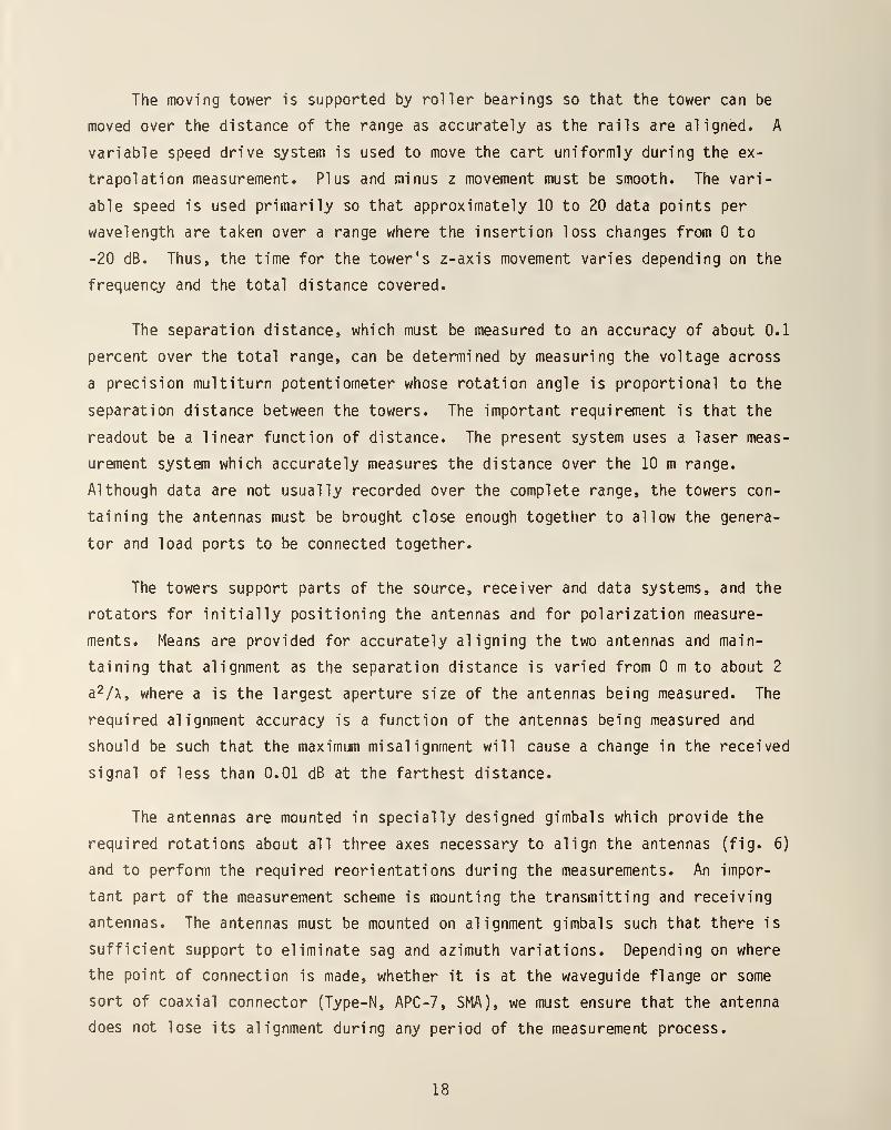
The antennas are mounted in specially designed gimbals which provide the

required rotations about all three axes necessary to align the antennas (fig. 6)

and to perfonn the required reorientations during the measurements. An impor-

tant part of the measurement scheme is mounting the transmitting and receiving

antennas. The antennas must be mounted on alignment gimbals such that there is

sufficient support to eliminate sag and azimuth variations. Depending on where

the point of connection is made, whether it is at the waveguide flange or some

sort of coaxial connector (Type-N, APC-7, SMA), we must ensure that the antenna

does not lose its alignment during any period of the measurement process.

18

tuSzoZj<<zzlU»-z<

•->

c0)

cCJ>•r—

gi «o

QC< (O

COT. c

5coc(U4->

-lO c<(E <Coo

•

C7>

19

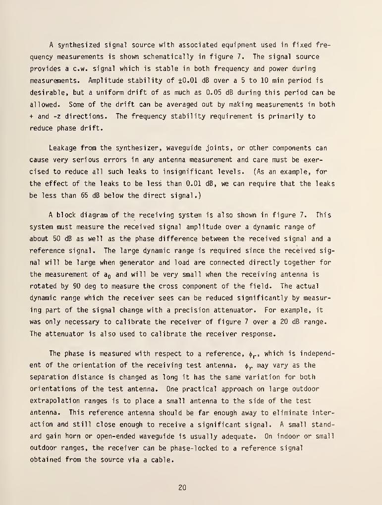
A synthesized signal source with associated equipment used in fixed fre-

quency measurements is shown schematically in figure 7. The signal source

provides a c.w. signal which is stable in both frequency and power during

measurements. Amplitude stability of ±0.01 dB over a 5 to 10 min period is

desirable, but a uniform drift of as much as 0.05 dB during this period can be

allowed. Some of the drift can be averaged out by making measurements in both

+ and -z directions. The frequency stability requirement is primarily to

reduce phase drift.

Leakage from the synthesizer, waveguide joints, or other components can

cause very serious errors in any antenna measurement and care must be exer-

cised to reduce all such leaks to insignificant levels. (As an example, for

the effect of the leaks to be less than 0.01 dB, we can require that the leaks

be less than 65 dB below the direct signal.)

A block diagram of the receiving system is also shown in figure 7. This

system must measure the received signal amplitude over a dynamic range of

about 50 dB as well as the phase difference between the received signal and a

reference signal. The large dynamic range is required since the received sig-

nal will be large when generator and load are connected directly together for

the measurement of ag and will be \/ery small when the receiving antenna is

rotated by 90 deg to measure the cross component of the field. The actual

dynamic range which the receiver sees can be reduced significantly by measur-

ing part of the signal change with a precision attenuator. For example, it

was only necessary to calibrate the receiver of figure 7 over a 20 dB range.

The attenuator is also used to calibrate the receiver response.

The phase is measured with respect to a reference, ())^, which is independ-

ent of the orientation of the receiving test antenna. ^^ may vary as the

separation distance is changed as long it has the same variation for both

orientations of the test antenna. One practical approach on large outdoor

extrapolation ranges is to place a small antenna to the side of the test

antenna. This reference antenna should be far enough away to eliminate inter-

action and still close enough to receive a significant signal. A small stand-

ard gain horn or open-ended waveguide is usually adequate. On indoor or small

outdoor ranges, the receiver can be phase-locked to a reference signal

obtained from the source via a cable.

20

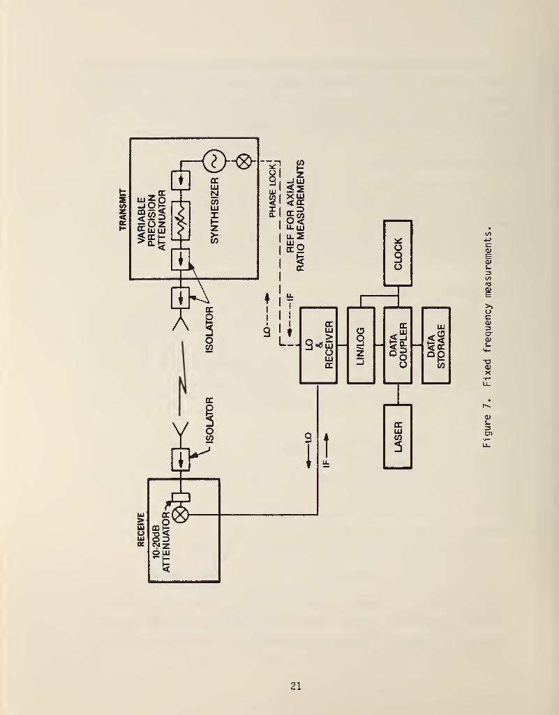
Mc:q;EdJ1-3CO"3

uc:

<uX

OJ

en

21

The receiver outputs are fed into the data system, which may be as simple

as an x-y recorder that plots the amplitude and phase as a function of the

separation distance. However, the requirements of accuracy, speed, and econ-

omy usually demand a digital system that records the data on magnetic tape or

disk in a format suitable for computer processing.

3. Measurement Procedures

Before the actual work on the range begins, the input reflection coef-

ficients for each antenna and for the generator and load ports are measured so

that corrections for mismatch errors can be made. This is very important when

one is attempting high accuracy measurements. A tuned reflectometer [19] or

network analyzer is normally used for this purpose.

3.1 Alignment of Antennas

Currently, there are two prescribed methods for aligning antennas. One

depends on the mechanical properties of the antenna while the other depends on

its electrical properties. Both methods will be described here. The goal of

the alignment procedure is to align the mechanical or electrical boresights of

the transmitting and receiving antennas with the reference z-axis of the

extrapolation range (fig. 5) and to provide a reference for the polarization

measurements.

Let us define three coordinate systems, one fixed to each of two antennas

and one fixed in space and referenced to the test range. Each antenna system

is defined with the boresight direction along the z-axis and the y-axis nomin-

ally along the major axis of the polarization ellipse. The exact location of

the axes is not critical but they must be clearly defined (fig. 5). The

reference, or space, coordinate system has its x-axis horizontal, the y-axis

vertical, and the z-axis along the center of the test range (fig. 6).

For the mechanical alignment method, the first step in the measurement is

to place the antennas in the prescribed orientations with respect to the

reference coordinate system. This is accomplished by first rotating the

antennas about their z-axes until their x-axes reference marks are horizontal.

This is easily done by viewing the antennas with a leveled transit placed

22

between the antennas. The transit is then aligned to determine the z direc-

tion of the range's rails. This is accomplished by placing fine wires across

the X- and y-axes of the transmitting horn, moving the cart in and out, and

aligning the transit so that there is no change in the position of the cross

hairs. A precision flat plate is then attached to the antenna aperture and a

precision mirror is centered on the plate. By using an autocollimator on the

transit, we then precisely align the antenna so that its z-axis is parallel to

the rails. The transit is then rotated about its y-axis precisely 180 deg,

and, in a similar manner, the receiving horn is aligned. An additional check

should be taken especially when the antennas are being aligned for polariza-

tion measurements, that is, when the antenna is rotated 360 deg about its

z-axis, the mirror must remain collimated and the intersection of the cross

hairs must remain constant.

In the electrical alignment method, first the x-axes of the antennas are

leveled with the transit just as in the former method. Now, however, the

towers are set for maximum separation, and the two antennas are alternately

rotated about their x- and y-axes to achieve maximum signal transfer. When

this is achieved the boresight directions for both antennas are coincident

with the reference z-axis, and the first stage of the alignment has been com-

pleted. The next step is to adjust the receiving antenna relative to its gim-

bal mount so that the z-axis of the mount is coincident with the boresight

direction of the antenna. This condition is achieved by rotating the antenna

180 deg about the mount axis, noting the shift in boresight direction, and

adjusting the antenna relative to the mount until a 180 deg rotation leaves

the boresight direction unchanged. Several iterations may be required.

3.2 Receiver Calibration and Determination of ag

When the alignment has been completed, the towers are moved close to-

gether so that the generator and load ports may be connected together. The

calibrated variable precision attenuator is then used to determine the linear

range of the mixer, calibrate the receiver response, and determine ag, the

input to the transmitter. The linear response range of the mixer is determined

by measuring the change in output signal, aB, resulting from a change in the

input precision attenuator, AL^ for various signal power levels. When oper-

ating at the correct power level, the difference (in decibels) between aB and

23

aL, will be a constant which is independent of the received power. During the

rest of the measurements the signal power level is maintained within the

linear region.

The receiver is then calibrated by systematically varying L^ over a to

20 dB range and recording the corresponding receiver output values. The re-

sulting calibration curve is used to correct the measured data.

Several steps are required in order to obtain the desired quantity,

|bo(d)/ao|, in terms of the receiver output, B{d), the change in the input

attenuator for the generator-load hookup, aL^, and certain mismatch factors.

The output amplitude meter measures relative signal changes, jbg/b|

, on a

logarithmic scale and the observed receiver output, B', is then given by

B'(d) = 20 logb^d)

b.(29)

The reference amplitude, b^, is essentially arbitrary but must remain constant

during the measurement. With the generator and load connected together, the

input attenuator is set on L^- and the receiver gain set for B' = 0. ' The ref-

erence amplitude is then given by [20]

h - g(30)

where bq is the wave amplitude that the generator would deliver to a matched

load. The antennas are now replaced with antenna m connected to the generator

and antenna n connected to the load. The input attenuator is reset to a new

value, Lf, which results in a new b^ given by b' = ab .

then 20 log |a| = AL-^. The input amplitude to antenna m is

b'

^0 ^(1 - tr)* m g^

If AL, = L. - L1 f^

and from eqs (29), (30), and (31) we obtain

bi(d)20 log = B'(d) - ALi - 20 log

(1 - r r^)

(1 - r^rJ^ g m^

(31)

(32)

24

aL^ is chosen so that B'(dj^-jp) = 0, where (i^-\^ is the minimum distance at

which data is to be taken. The towers are now moved slowly apart and the re-

sulting amplitude B'{d) and phase (j)'(d) data recorded as a function of dis-

tance.

The receiving antenna is then rotated about its z-axis by 90 deg, the

output attenuator changed by AL2, if necessary, to restore the signal level at

the receiver to its previous range, and the amplitude B"(d) and phase ^"{d)

data again recorded as a function of distance. This measurement sequence is

repeated for all three antenna pairs to provide the necessary data for the

extrapolation calculations and solution of the three-antenna equations.

The generator and load connections are a very important part in the meas-

urement process and great care must be taken to assure repeatable, accurate

measurements in the hookups. For example, an error in the generator-load

hookup translates directly into an error in the average gain of the antenna

pair being measured. (Typically, generator-load measurements repeat to within

0.02 dS.) The generator-load connection is necessary to determine absolute

gain which accounts for the ohmic loss of the antennas. This is in contrast

to measuring the directivity of an antenna, estimating the ohmic loss and cal-

culating the absolute gain, a procedure used in some laboratories.

A potential source of error often appears at the junction of the coaxial

cable and the coax-to-waveguide adapter. Care must be taken that the connec-

tor is neither tightened too tightly, damaging the center pin or too loosely

so that the connection can work itself free. A solution to this problem is

the use of torque wrenches and the introduction of strain relief loops at the

connector joints. Strain relief loops eliminate many problems which occur

with movement of the input and output assemblies during generator-load hook-

ups, since the connection is isolated from the general cable movement. Even a

single loop securely fastened to the coax-to-waveguide assembly or accompany-

ing waveguide piece provides adequate protection from connector problems

(fig. 8).

Another area where problems often occur is the transmission cable itself.

Depending on what types of cables are used, e.g. (RG 214-U, RG 9-U, 0.358 cm

(0.141 in) diameter semi-rigid, the following should be verified about the

cable:

25

(a)Isolator

Coiledcable

Coaxialconnector

(b)Isolator

Isolator

(c) (d)

Isolator

Figure 8. Steps in making a strain relief loop to minimize cable movement atconnector joints.

1. It has the appropriate frequency response for the measurement.

2. It has stable (preferably low) loss.

3. It has the durability to withstand occasional bending and movement.

4. It is firmly attached to the connector, primarily to minimize signal

leakage.

5. It has durable connectors to insure repeatability.

Depending on the previous usage of the cable, it is always good practice to

visually inspect each cable and to test it electrically before installing it

in the system.

The assembly of waveguide components can also present problems to the

technician where leakage and connection repeatability d^vo. concerned. All

waveguide joints must be put together in a consistent manner. Care must be

taken to minimize leakage by using proper shielding of the joints with copper

26

tape or some type of foil. We should also ensure that any waveguide system

have sufficient support that the torque on any waveguide component is mini-

mized.

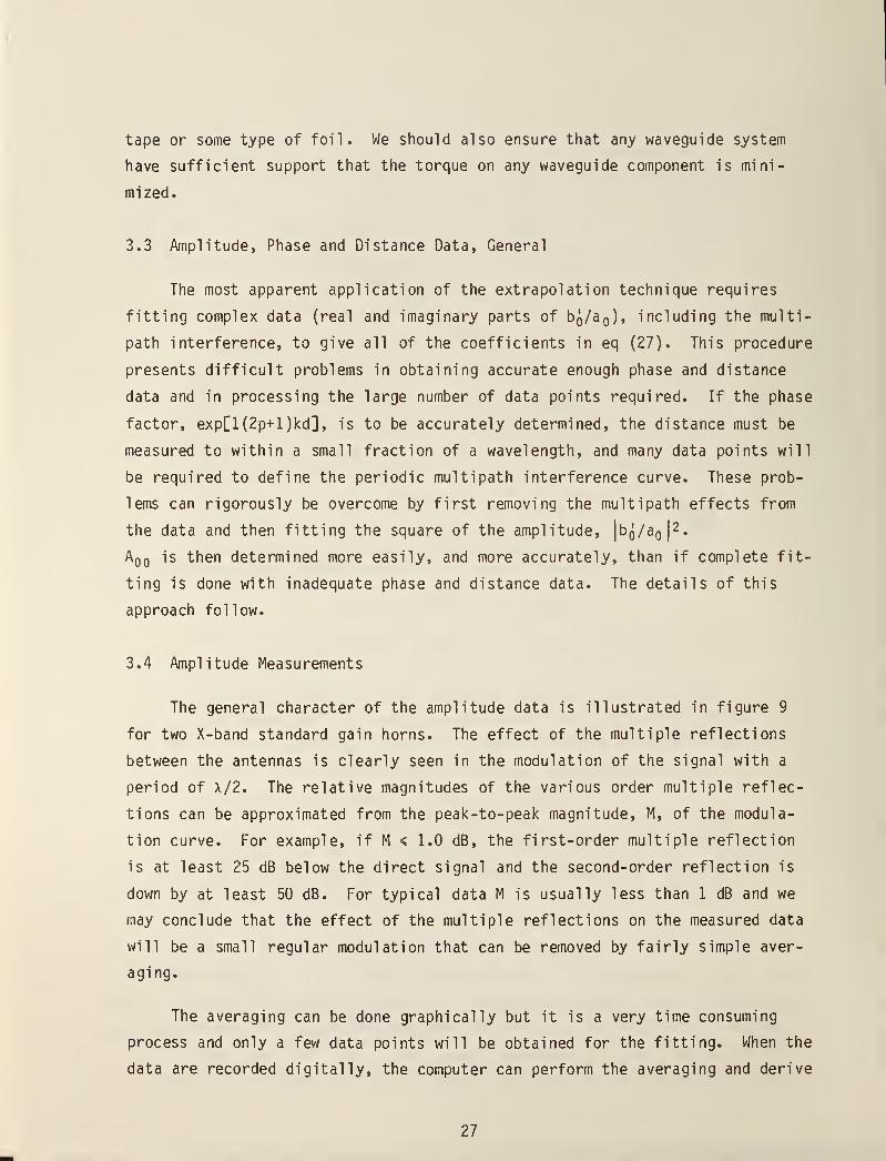
3.3 Amplitude, Phase and Distance Data, General

The most apparent application of the extrapolation technique requires

fitting complex data (real and imaginary parts of bg/ao), including the multi-

path interference, to give all of the coefficients in eq (27). This procedure

presents difficult problems in obtaining accurate enough phase and distance

data and in processing the large number of data points required. If the phase

factor, exp[l(2p+l)kd], is to be accurately determined, the distance must be

measured to within a small fraction of a wavelength, and many data points will

be required to define the periodic multipath interference curve. These prob-

lems can rigorously be overcome by first removing the multipath effects from

the data and then fitting the square of the amplitude, |bo/ao|^.

Ago is then determined more easily, and more accurately, than if complete fit-

ting is done with inadequate phase and distance data. The details of this

approach follow.

3.4 Amplitude Measurements

The general character of the amplitude data is illustrated in figure 9

for two X-band standard gain horns. The effect of the multiple reflections

between the antennas is clearly seen in the modulation of the signal with a

period of X/2. The relative magnitudes of the various order multiple reflec-

tions can be approximated from the peak-to-peak magnitude, M, of the modula-

tion curve. For example, if M < 1.0 dB, the first-order multiple reflection

is at least 25 dB below the direct signal and the second-order reflection is

down by at least 50 dB. For typical data M is usually less than 1 dB and we

may conclude that the effect of the multiple reflections on the measured data

will be a small regular modulation that can be removed by fairly simple aver-

aging.

The averaging can be done graphically but it is a very time consuming

process and only a few data points will be obtained for the fitting. When the

data are recorded digitally, the computer can perform the averaging and derive

27

lOr

Figure 9.

90 no 130 150 170 190

SEPARATION DISTANCE (cm)

Extrapolation data for two X-band standard gain horns.

many more points in a much shorter time. We usually record 10 to 20 data

points over each cycle of the interference pattern, and the computer averages

over a fixed number of points or computes a running average. Averaging is

typically accomplished over an integral multiple of half wavelengths.

A third alternative is to use a low-pass filter in the output section of

the receiver to filter out the modulation produced by the multiple reflect-

ions. The modulation frequency can be controlled by the speed of the tower,

and is given by fp = 2V/nX, where f^ is the frequency resulting from the nth-

order reflection, V is the velocity of the tower, and \ is the wavelength of

the rf signal. This procedure works very well at short wavelengths and for

phase-locked receivers which have narrow bandwidths. The averaging is then

accomplished automatically without any computations. Figure 10 shows the

appearance of the modulation at a very slow tower motion and the automatic

averaging accomplished at a moderate tower speed. The individual cycles of

the multipath are not resolved here because of the short wavelength (=5 mm).

28

CQ-a

CO

o

MULTIPATHTOWER MOVING SLOWLY

AVERAGE CURVETOWER MOVING 0.5 M/S

J I I I I I I t

8 12 16 24

SEPARATION DISTANCE (m)

Figure 10. Extrapolation data showing multipath interference and averagedcurve for two 45 cm (18 in), millimeter-wave, parabolic-reflectorantennas.

14,-

16 24 32 40

SEPARATION DISTANCE (m)

48 56

Figure 11. Averaged extrapolation data for the same antenna as in figure 8.

29

The result of this process is a number of points on an averaged curve,

such as in figure 11. Since all orders of multipath signals have been

removed, this received signal can be represented by the first series of

eq (27), giving

-ikd^(d)'' (1 - W) e \l %2 ^3

Since only the amplitude is to be fitted, we take the square of the absolute

value of eq (33) and obtain

bi(d)d2 a;, AI2 Ai3

^0

where

A^o = AooAoo = hoop

Aoi = AoqAoi + AooAoi (35)

A()2 " A00A02 + A00A02 *" AqiAoi.

(The bar denotes the complex conjugate.)

It is apparent that the coefficient which determines the far-field

properties, Aqq, is still determined from the first term in the new series.

The received signal will also be modulated by ground reflections when

present. This effect can be distinguished from the multiple reflections by

its longer modulation period, P^, which also increases with the separation

distance. For example, if the ratio of antenna height to separation distance,

h/d, is » 1, P^ = X; for h/d = 1, P^ = 2X; and for h/d = 1/4, P^ ^ lOx. If

ground reflections are present h/d must be large enough to result in several

modulation periods over the measurement distance. This effect can then also

be averaged out graphically and by computer, or by simply fitting the data

with a low-order series.

30

The spacing of the data points is chosen to give between 1000 and 3000

approximately equally spaced points over the measurement interval. We have

found it best to record data for repeated runs over the same measurement

interval with the tower moving in opposite directions. This tends to random-

ize amplitude drifts or other short term changes, and is, therefore, prefer-

able to relying on a single run.

The guidelines for choosing a particular distance interval to operate

over depend on the types of errors in the data and will be discussed in the

section on error analysis. However, at the present stage of development, it

appears that the maximum distance, djy,^^, should be at least a^/x, but not so

great that large ground reflections occur. The minimum distance, d^^^-^, is

chosen small enough so that dj^^ax^^min ^ ^» ^^^ ^^ should be large enough that

three to six coefficients will accurately fit the data [see below eq (41)].

The distance interval which meets these guidelines will depend on the antennas

being measured, but will be approximately between 0.2 (a^/x) and 2 (a^/x).

Another criterion is that there be at least 10 dB total variation in signal

level over the distance interval.

3.5 Phase Measurements

As stated in the last paragraph in section 2.2, we generally calibrate

three antennas that are nominally polarization matched. Using this approach,

we can determine to high accuracy the gain of the antennas without need for

phase measurements (section 5.2). Axial ratios and tilt angles are then

determined using the improved polarization technique described in section 7.

Phase measurements have been used to determine gain and polarization param-

eters, however, and are included here for tutorial purposes and completeness.

Phase-versus-di stance measurements have been used to reduce the effects of

ground reflections when determining gains for broadbeam antennas (appendix A).

Since polarization and gain are independent of any phase factor common to

both Xp and Y^, only the relative phase difference between D^^^ and d'^^ need be

measured. This is given by [eqs. (19) and (20)]

D" ,. b;:(d)nm _ lim ^^„ "^ ' (26)

A4) = arg -rn— =.

arg . , y ,v \^°)^nm ^ D d-*-" bo(d)

nm "

31

and is determined by measuring the phase of bo(d) and bo(d) relative to a com-

mon reference, and then computing the phase difference as a function of dis-

tance. Some averaging of multipath effects and extrapolation of the phase

data also required, and this is yery similar to the analysis of the amplitude

data.

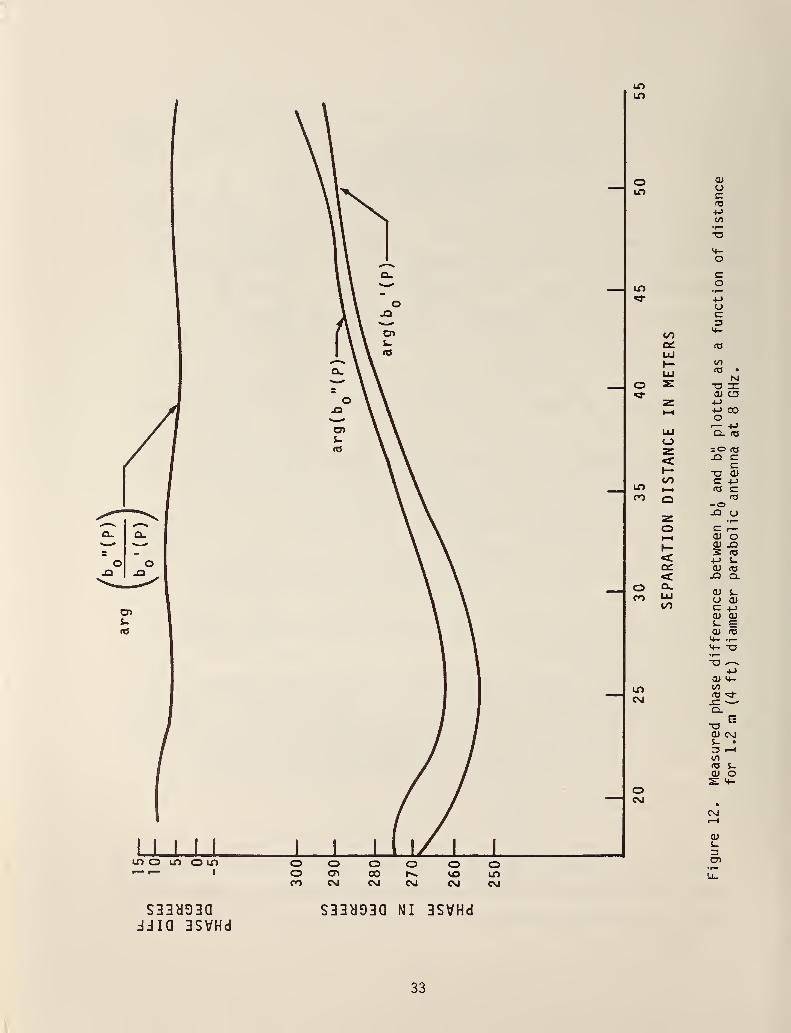
Figure 12 shows the phase differences for an antenna pair plotted as a

function of reciprocal distance, and illustrates the asymptotic character as d

becomes large.

4. Numerical Techniques for Antenna Gain and Polarization Measurements

When the measurements have been completed, the data are analyzed to

determine Ago and the phase difference for each orientation for each antenna

pair (sect. 3.5, paragr. 1). The main tasks of the computer processing are to

read the data from magnetic tape, fit the data to a power series, and make

various plots and tabulations of the measured data and the fitted curves.

The first step in this computer processing is the averaging discussed in

a previous section v/hich eliminates the effects of multiple reflections. The

amplitude data are then modified to account for the receiver calibration,

atmospheric attenuation, impedance mismatch, and the change in the input

attenuator [aL^ in eq (32)].

The independent and dependent variables, u and v, to be used in the

fitting are next computed from the amplitude and distance data, u is equal to

the reciprocal distance scaled by the factor a^/x, and is given by

^d

•

This scaling is done so that the computer generated plots for any antenna will

have a distance scale in units of a^/x. It is strictly a matter of conveni-

ence in interpreting the graphs and has no effect on the final result.

If the amplitude has been recorded in voltage or decibels, it is con-

verted to a power ratio and multiplied by d^ to give the dependent variable v.

32

C7)

rO

D>

(O

I I I I I I I

in

o

in

oCVJ

LD O LO o to o o o o O O1 o a\ 00 r^ VO in

ro CO OJ CM OJ C\i

(J

+->

coin

«a-

oo

o

<4-

Q^ fOLlI

H- 1/)

oUJ N

T3 :e^ cu oz •!->

•—

•

-(-> 00o1— 4->

LU Q. (OOz = fO

<1— XJ <ut/) C +J

in t—

1

fC cCO Q -o

Z •r—o c: I—HH OJ ot— 0) J2

< -»-> J-cc: O) fT3

<: J3 Q.oCO LU CJ OJ

to c: 4->

S- E

M- -O

O) <+-

13 «vt-

szQ.

EoO) CVJJ- •

tofO s_O) o

CSJ

CD

S33b93adJia BSVHd

S33y93a NI 3SVHd

33

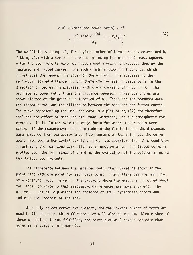
v(u) = (measured power ratio) • d^

b'o{d)d e-^'^^ (1 - r^r^) 2 (37)

The coefficients of eq (34) for a given number of terms are now determined by

fitting v(u) with a series in power of u, using the method of least squares.

After the coefficients have been determined a graph is produced showing the

measured and fitted curves. One such graph is shown in figure 13, which

illustrates the general character of these plots. The abscissa is the

reciprocal scaled distance, u, and therefore increasing distance is in the

direction of decreasing abscissa, with d = «> corresponding to u = 0. The

ordinate is power ratio times the distance squared. Three quantities are

shown plotted on the graph as a function of u. These are the measured data,

the fitted curve, and the difference between the measured and fitted curves.

The curve representing the measured data is a plot of eq (37) and therefore

includes the effect of measured amplitude, distance, and the atmospheric cor-

rection. It is plotted over the range for u for which measurements were

taken. If the measurements had been made in the far-field and the distances

were measured from the approximate phase centers of the antennas, the curve

would have been a horizontal straight line. Its departure from this condition

illustrates the near-zone correction as a function of u. The fitted curve is

plotted over the full range of u and is the evaluation of the polynomial using

the derived coefficients.

The difference between the measured and fitted curves is shown in the

point plot with one point for each data point. The differences are amplified

by a constant factor (given in the captions above the graph) and plotted about

the center ordinate so that systematic differences are more apparent. The

difference points help detect the presence of small systematic errors and

indicate the goodness of the fit.

When only random errors are present, and the correct number of terms are

used to fit the data, the difference plot will also be random. When either of

these conditions is not fulfilled, the point plot will have a periodic char-

acter as is evident in figure 13.

34

^ 0.20CVJ

a:

o<cI-toI—

«

oXo

3O

0.16^

0.12-

— LEAST SQUARE FIT TO DATA

— MEASURED DATA

0.8 1.6 2.4 3.2 4.0

RECIPROCAL NORMALIZED DISTANCE ^-^

Figure 13. Measured-data, two-term polynomial fit, and residuals for X-bandconical horn (gain « 22 dB).

The correct number of terms to use in the polynomial fit is determined by

using the Snedecor-Fisher F-test of statistical significance [21]. To use

this test, a set of N data points is fitted with a sequence of polynomials of

increasing order, and the residuals, defined as the sum of the squares of the

differences between the measured and fitted curves, are computed for each set

of coefficients. If we denote the residuals for the series with n coeffi-

cients by r^, then the nth coefficient is significant if

(r,-r )(N-n)^ n-1 n''^ ' r

'n- > F(1,N). (38)

Values for F(1,N) can be found in tables of percentiles of the F distribution.

For the present case where N > 100, F(1,N) is taken to be about 5. The value

of F^ is computed for each trial series and printed out with the results and

35

if it is greater than 5, the last term in the series is significant. The

series which gives the best significant fit is terminated with the highest

order coefficient which is significant, and the first coefficient of that

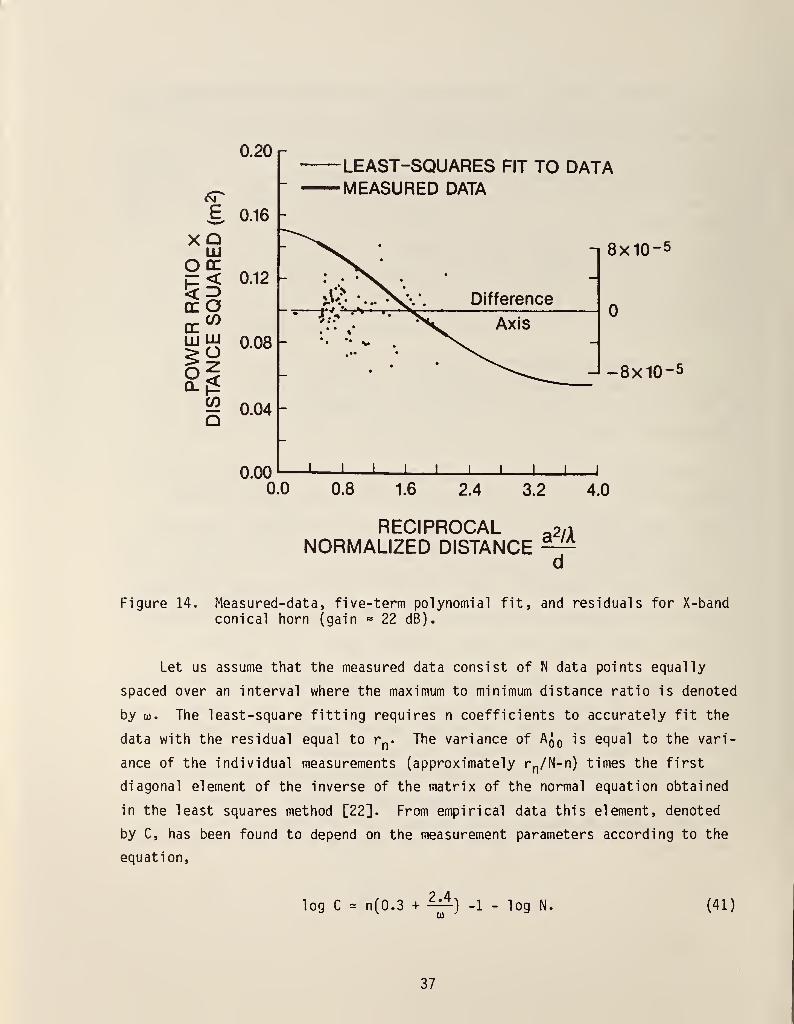
series is Aqq. Figure 14 shows the graph of the 5-term series that was deter-

mined to be the best fit where all coefficients were significant. There is

still a very small (±0.01 dB) periodic character to the difference plot which

is due to residual errors. It is similar in character to ground reflections,

but has a longer period, and if a number of cycles are present in the data, it

will have a very small effect on the determination of Aqq.

Because only the relative phase between D^^ and D^j^ is required we may

arbitrarily assign a deg phase to 0^1^^, and we then have

^ A^oD' = -o--r (39)nm 2TTik ^ '

where Aqq = Aqq for notational convenience. From data taken with the same

antenna pair after rotation of the receiving antenna about its axis [eq (20)],

we obtain a new series and therefore a new constant coefficient denoted by

Aqq. d;;^ is then given by

/ Ann "iA<J>

°™ =^^ ™ («'

The measurement and fitting procedures are carried out for the three antenna

pairs which yield the six D^^'s required to solve eqs (22) through (25) and

(14) through (18) for the gain and polarization of each antenna.

5. Error Analysis

The errors that have the largest effect are those which vary with dis-

tance, because extrapolation can amplify the effect of small errors in the

data to significant errors primarily in Aqq. The magnitude of this effect is

dependent on the character of the measured data and the error function. The

results presented here will be for typical antennas and error functions which

are usually a worst-case upper bound type. By typical antennas we mean horn

and reflector type microwave antennas.

36

0.20

£ 0.16

XQ

p<ccO

LU lU

2i

0.12

0.08

^ 0.04

0.00

LEAST-SQUARES FIT TO DATAMEASURED DATA

-^ 8x10-5

-•-8x10-5

J L J L

0.0 0.8 1.6 2.4 3.2 4.0

RECIPROCAL ^2/1NORMALIZED DISTANCE ^^

Figure 14. Measured-data, five-term polynomial fit, and residuals for X-bandconical horn (gain « 22 dB).

Let us assume that the measured data consist of N data points equally

spaced over an interval where the maximum to minimum distance ratio is denoted

by 0). The least-square fitting requires n coefficients to accurately fit the

data with the residual equal to r^. The variance of Aqq is equal to the vari-

ance of the individual measurements (approximately r^/N-n) times the first

diagonal element of the inverse of the matrix of the normal equation obtained

in the least squares method [22]. From empirical data this element, denoted

by C, has been found to depend on the measurement parameters according to the

equation.

log C = n(0.3 +— ) -1 - log N. (41)

37

This relationship requires that N 5 100, w > 4, and preferably that n < 6 if

the effects of random error are to be minimized. Under these conditions, the

standard deviation in D^^ due to random error is about 0.05 dB.

The character of errors [23,24] due to receiver nonlinearity, range mis-

alignment, instrument drift, and atmospheric attenuation uncertainty are all

quite similar. That is, error in the amplitude data will be essentially zero

for the minimum distance and can be bounded by a monotonically increasing

error with a maximum value of e^ at the maximum distance. The continuously

increasing error is a worst-case situation, and the actual error may in fact

oscillate about zero which results in a smaller error in Aqq.

For the worst-case situation, the resulting error in D^^ due to one

source with a maximum error of e^ is approximately Sn = 2 e . The values of

e^^ for each source (receiver, alignment, etc.) must be estimated for each

measurement situation, and are typically no greater than 0.02 to 0.05 dB.

Phase errors are caused by receiver error, antenna alignment error, and

multipath signals. The largest phase errors will result when two highly

linearly polarized antennas are being used. In this case, small boresight

errors or inaccuracy in the 90 deg rotation can result in phase errors of tens

of degrees. Fortunately, the phase is not as important in calculating gain

and polarization characteristics for this case. When one antenna is linearly

polarized and the other is circularly polarized, alignment is not nearly as

critical, and the phase of DJ^j^ can be determined with errors of 1 deg or less.

5.1 Propagation of Errors to Gain and Polarization Parameters

For the purposes of this discussion, we will consider D^^ and D^^^ to be

quantities whose values and uncertainties are known (since they are \/ery

simply related to Aqq* Aqq, and A(j>) and determine the effect of these uncer-

tainties on the computed gain and polarization parameters. This will be done

for two-antenna combination sets that represent the situation for almost all

measurements.

38

5^2 Three Nominally Linearly Polarized Antennas

It is assumed that the axial ratio for all three antennas is at least

20 dB and that each antenna is oriented such that its principal component is

approximately along the y-axis. Equation (25) for the linear components upon

substituting eq (22) is then approximately

Yi = -i /"DilDiI ^ "^1 Di2 Di3 D23 -YiAi

d 12 m13 D 23(42)

where A^ is the quantity within the brackets of eq (42). The gain, polariza-

tion ratio, axial ratio, and tilt angle are then

4iTk2

^1 =1 - IS 00

023^13

D'23(1 +

K\'-)} (43)

and

Pa = --? ^1 = -2/Ini(Aj Ti =Re(A^)

(44)

For nearly linearly polarized antennas, A will have little effect on the

gain, and the error in G will be primarily due to the errors in the |Dj!,^|s.

If we let c^^ be the error in decibels for each of the measured quantities,

then the resulting error in the gain will be

- ei2 + ei3 " ^23'

For the case of three antennas with approximately equal gains, the systematic

error in each e^^^ will be ^ery nearly the same. If we denote the systematic

component by e^ and the random component by e^, then for this case

e = e + /3 e .

g s r

For the axial ratio and tilt angle, errors in A have the major effect.

If we denote the amplitude and phase of the ratios in A as

ieD"nm

D'nm

= ci„^ enm

nm(45)

39

(46)

(47)

then the errors in A and t will be given by

A?

dAi =2 (^12 COS9i2Ci6i2 + ^13 COS9i3d9i3 - 323 COSe23d923

+ sin9i2dai2+ sin9i3dai3 - sin923da23)

and

dx = ai2 sin9i2d9i2 + ^13 sin9i3d9i3 - 823 sine23d923

- cos9i2dai2 - cos9i3dai3 + COS923da23.

5.3 Two Nominally Linearly and One Nominally Circularly Polarized

Antenna Combination

The linearly polarized antennas are again oriented with their principal

components approximately along the y-axis, and we assume that antenna number 3

is nearly left circularly polarized. When either antenna 1 or 2 is used with

number 3, the 90 deg rotation about the z-axis will result in a very small

amplitude change, and approximately 90 deg phase change. Therefore,

n" n" n"U12 L)i3 U23

D|^= 5i2. "Di7=^' ^ "^is. DJ7" ^

" ^23. (48)

where the 6's represent the small deviation from exactly linear and circular

polarization. An analysis similar to that in the previous section shows that

the left and right components of Sio(O) are given approximately by

4 Dl3D^3 ^ L3

•ITL3 = ± p-— , R3 = + ^ / - 613623, (49)

and that the gain, circular polarization ratio, axial ratio, and tilt angle

are approximately

Gs' i. 1 2 T^TT (50)^ Pool ^ P12

and

40

C ^P^ = o A = - (1 + I/613623I) T = 2 ,

where ^^-^ and isf2^ ^re the phase angles of 5^3 and 623*

The gain calculation here is similar to the previous case, where only the

large quantities were significant. There is once again some cancellation of

the systematic error components for this case, but since five rather than

three quantities are involved, the effect of random error is larger. The gain

error is given by e = s + /3" e where e and e are the systematic and^•^gs r sr "^

random errors in each of the Dp(,i's.

If two similar linear antennas are used, then 613 = 623 and for this case

the error in the axial ratio is

dA = (2ai3 + 2 sineis) dai3 + 2ai3 cosei3dei3. (51)

Since 613 = -90° and 3^3 = 1, errors (da^s « 0) in the measured quantities do

not strongly affect the calculated axial ratio.

The accuracy of tilt angle is very dependent on experimental errors,

especially for highly circular polarization. The angles 613 and 623 are

related to the measured ratios by

, 1 + ai3 sinei3 1 ^ "*" ^23 sin923

and the error in <|>i3is

- cosej3da^3 + (afg + a^j sin0^3]d9i3

^*i3 = r.a23.2a,3Sin9,3 *^''^

The tilt angle error is given by

d(()i3 + d(t.23 ,^^^dT =

2f(54)

and can be quite large for nearly circular polarization when 613 and 623 are

close to -90 deg and ai3 and a23 are nearly 1.

41

6. Measurement Examples

The extrapolation technique has been used on a number of antennas at fre-

quencies from 1 to 65 GHz. For some of these, gain measurements have been

made using different techniques and the results have always agreed to within

±0.15 dB. In one comparison, the gain of a multimode X-band horn was measured

by NBS using both the extrapolation technique and a near-field scanning tech-

nique. The Jet Propulsion Labs also determined the gain of the horn [25] from

far-field pattern measurements. The results of all three measurements were

within ±0.10 dB of each other.

For some measurements on pyramidal horns, the proximity corrections

obtained from the extrapolation measurements had been compared with theoret-

ical expressions based on the geometry of the horn and assumed field distri-

butions. There has been fairly good agreement with the results of Chu and

Semplak [26] for a limited number of comparison.

The results of measurements on two different antenna sets will now be

described. These will illustrate the present accuracy capabilities for

antenna gain and polarization measurements.

6.1 X-Band Standard Gain Horns

This antenna set consisted of two commercial standard gain horns with

nearly linear polarization and one horn with nominally circular polarization.

The measurement frequency was 7.250 GHz, and a^/x for the circularly polarized

horn was about 1.33 m. Measurements were made over a distance range from 1.2

to 2.8 m for the three antenna combinations and the extrapolation procedure

carried out to give the results shown in table 1 which also includes the 3a

error estimates. The error estimates for atmospheric loss uncertainty are

obtained from reference [27]. The measured data and error estimates then

result in the following calculated quantities for the circularly polarized

horn:

Gain = 21.32 dB ± 0.11 dB

Axial ratio = 1.34 dB + 0.05 dB

Tilt angle = - 59.3° + 2.5°

42

Table 1. Data and errors for X-band antennas.

Linear #1

and C.P.Linear #2and C.P.

Linear #1and #2

Amp. (dB) 3.60

D'

Phase (deg) 0.0

3

0,

.69

.0

3.29

0.0

Amp. (dB) 3.28D"""^

Phase (deg) 262.1

3,

262,

.37

.5

-2.30

275.0

Source of Error 1Error i" ^m,(dB)

Impedance mismatch 0.01

Attenuator calibration 0.01 -

System drift and receiver nonlinearity 0.05

Atmospheric loss uncertainty 0.00

Antenna alignment 0.01

Distance nonlinearity 0.04

Quadrature sum systematic errors 0.06

Random errors 0.03

6.2 V-Band Reflector Antennas

These were linearly polarized, 45 cm diameter reflector antennas.

Antennas 1 and 2 were equipped with focal point feeds and #3 has a Cassegrain

feed. At the test frequency of 57.5 GHz, a^/x was 40 m. Extrapolation data

was taken over a range from 10 to 60 m on the NBS outdoor range with the

results shown in table 2.

From these data the antenna parameters and error estimates were deter-

mined to be

Antenna #1 #2 #3

Gain (dB)

Axial ratio (dB)

Tilt angle (deg)

46.61 ± 0.23

35.1 ± 2.4

87.6 ± 0.2

46.59 ± 0.23

43.7 ± 3.3

88.6 ± 0.1

46.26 ± 0.23

26.7 t 1.2

-89.0 ± 0.5

43

Table 2. Data and errors for mm-wave antennas.

#1 and #2 #2 and #3 #1 and #3

Amp. (dB) -26.06 -26..23 -26.21

Phase (deg) 0.0 0..0 0.0

Amp. (dB) -37.56 -40,.19 -40.49D"

Phase (deg) 20.0 280..0 310.0

Source of Error [irror in D,^(dB)

Impedance mismatch 0.01

Attenuator calibration 0.006

System drift and receiver nonl inearity 0.05

Atmospheric loss uncertainty 0.10

Antenna alignment 0.03

Distance nonlinearity 0.04

Quadrature sum systematic errors 0.12

Random errors 0.07

7. Improved Polarization Measurements

Absolute polarization parameters have been obtained in the previous sec-

tions using a three-antenna measurement technique [12,13,28]. By a modifica-

tion of this approach [29], the accuracy of the results are significantly

increased, and the measurements are easier to perform. Using this technique,

it is possible to accurately calibrate polarization standards which have axial

ratios greater than 40 dB. These standards are an important factor in the

measurement of antenna systems which require high polarization purity. This

work demonstrates the power and utility of using complex rather than real

polarization parameters in formulating polarization problems.

As we did before and repeat here for convenience, let us define three

coordinate systems, one fixed to each of two antennas and one fixed in space

and referenced to the test range. Each antenna system is defined with the

boresight direction along the z-axis and the y-axis nominally along the major

44

axis of the polarization ellipse. The exact location of axes is not critical

but it is important that they be clearly defined. The reference, or space,

coordinate system has its x-axis horizontal, its y-axis vertical, and its z-

axis along the center of the test range. Now place the source antenna on the

test range so that its axes are coincident with the reference system. The

receiving antenna has its boresight {+z-axis) along the reference -z-direc-

tion, and is rotated about the reference z-axis into two orientations where

measurements are performed (fig. 15). In the first orientation the +y-axes of

the antennas are in the same direction, and in the second the -x of the

receiving antenna is in the same direction as the +y of the source antenna.

The coupling equations for these two orientations [eq (21)] are respectively

X1X2-Y1Y2 = DI2, (55)

X1Y2+X2Y1 = D'i2 (56)

where the D's are proportional to the complex received signals, and X^ and Y^

are the x- and y-components of the plane-wave spectrum transmitting

characteristic Sio(9><^) of the source antenna in the direction 9 =(j)

= 0.

X2 and Y2 are similar quantities for the receiving antenna. Sjo(9j<I>) is

simply related to the far-electric field E, [eq (9)] and since we will only be

concerned here with ratios of the components, the formulation can be thought

of as being in terms of either _E or _S.

In eqs (55) and (56) we have assumed that the receiving antenna is recip-

rocal and expressed all antenna parameters in terms of transmitting proper-

ties. This is not necessary to the technique, but it makes the notation more

concise aTid consistent with previous material [13].

The approach in the three-antenna measurement is to repeat this procedure

for all three antenna pairs, measure the D^^^'s and solve the resulting six

equations for the linear components X^ and Y^, the right and left circular

components R^ and L , and obtain gain, complex linear polarization ratio p^,

complex circular polarization ratio p^,, axial ratio A, and the tilt angle t.

These polarization parameters are related by the equations [eqs (13) through

(18)]

45

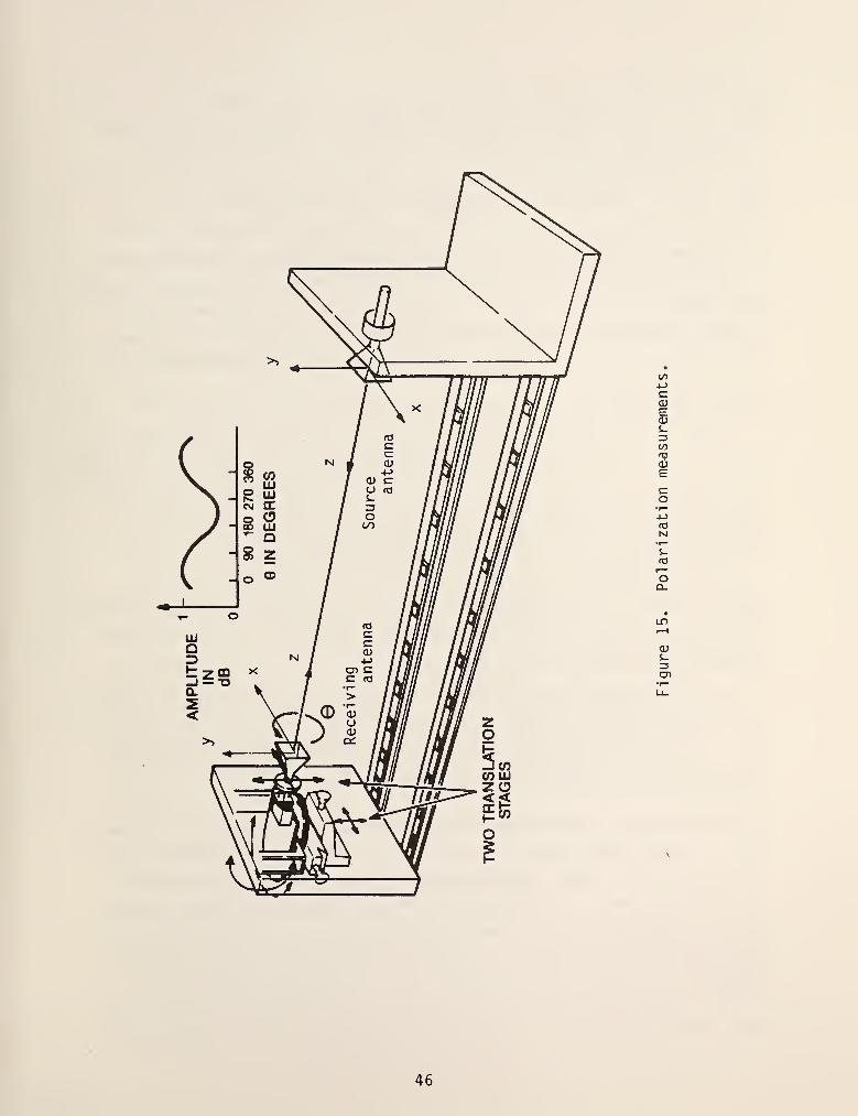
00-t-J

O)EO)S-r3w"?C3J

Eco-(->

03N•r—

S-

'oQ.

46

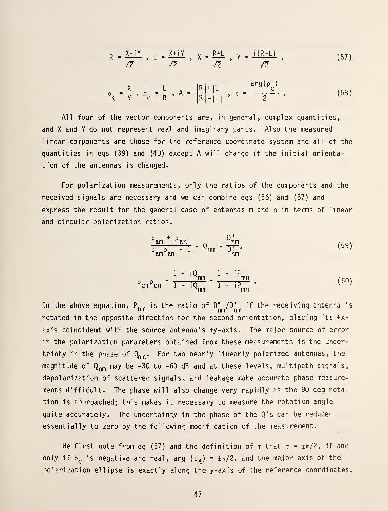
R=MV.L=^.X = B±L. Y=lim, (57)fl /2 jz n

^ 'Y • ^c " R • * ' "fRnrt ' ' " "2"" • '^^'

All four of the vector components are, in general, complex quantities,

and X and Y do not represent real and imaginary parts. Also the measured

linear components ^v^ those for the reference coordinate system and all of the

quantities in eqs (39) and (40) except A will change if the initial orienta-

tion of the antennas is changed.

For polarization measurements, only the ratios of the components and the

received signals are necessary and we can combine eqs (56) and (57) and

express the result for the general case of antennas m and n in terms of linear

and circular polarization ratios.

(59)p« + pmp p

%x\

T= ^nm=

D"nm

D' '

nm

cm^cn

1

" T+

^^nm

i^nm

1

r- iP

mn

mn(60)

In the above equation, P„^ is the ratio of D" /D' if the receiving antenna is^ nm nm nm

rotated in the opposite direction for the second orientation, placing its +x-

axis coincident with the source antenna's +y-axis. The major source of error

in the polarization parameters obtained from these measurements is the uncer-

tainty in the phase of Q^^^^. For two nearly linearly polarized antennas, the

magnitude of Q^j^ may be -30 to -60 dB and at these levels, multipath signals,

depolarization of scattered signals, and leakage make accurate phase measure-

ments difficult. The phase will also change very rapidly as the 90 deg rota-

tion is approached; this makes it necessary to measure the rotation angle

quite accurately. The uncertainty in the phase of the Q's can be reduced

essentially to zero by the following modification of the measurement.

We first note from eq (57) and the definition of t that x = ±Tr/2, if and

only if p^ is negative and real, arg (p^) = ±it/2, and the major axis of the

polarization ellipse is exactly along the y-axis of the reference coordinates.

47

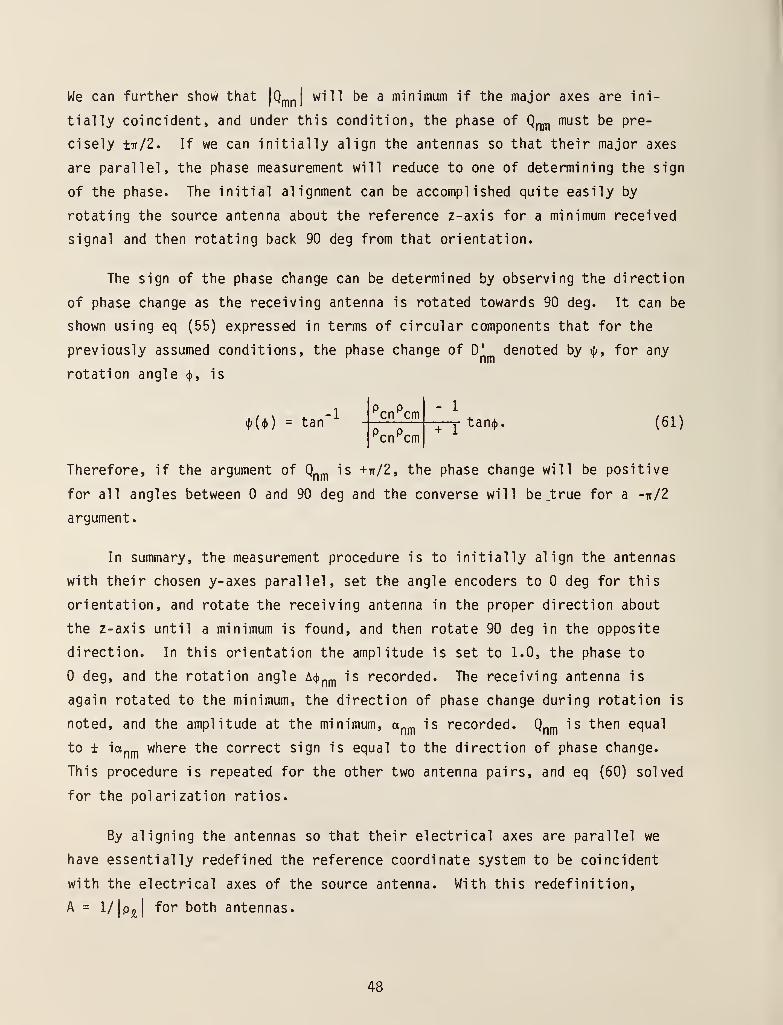
We can further show that \Q^y\\ ^^^^ ^^ ^ minimum if the major axes are ini-

tially coincident, and under this condition, the phase of Q^^^^ must be pre-

cisely Itt/Z. If we can initially align the antennas so that their major axes

are parallel, the phase measurement will reduce to one of determining the sign

of the phase. The initial alignment can be accomplished quite easily by

rotating the source antenna about the reference z-axis for a minimum received

signal and then rotating back 90 deg from that orientation.

The sign of the phase change can be determined by observing the direction

of phase change as the receiving antenna is rotated towards 90 deg. It can be

shown using eq (55) expressed in terms of circular components that for the

previously assumed conditions, the phase change of D' denoted by ij;, for any

rotation angle (t), is

- 1

ij;((j)) = tan'P^cn^cmP

"^cn^^cm+ 1

tan({>. (61)

Therefore, if the argument of Q^^ is +tt/2, the phase change will be positive

for all angles between and 90 deg and the converse will be ^true for a -ir/2

argument.

In summary, the measurement procedure is to initially align the antennas

with their chosen y-axes parallel, set the angle encoders to deg for this

orientation, and rotate the receiving antenna in the proper direction about

the z-axis until a minimum is found, and then rotate 90 deg in the opposite

direction. In this orientation the amplitude is set to 1.0, the phase to

deg, and the rotation angle ^^^ is recorded. The receiving antenna is

again rotated to the minimum, the direction of phase change during rotation is

noted, and the amplitude at the minimum, a^^ is recorded. Qp^ is then equal

to ± ittp^ where the correct sign is equal to the direction of phase change.

This procedure is repeated for the other two antenna pairs, and eq (60) solved

for the polarization ratios.

By aligning the antennas so that their electrical axes are parallel we

have essentially redefined the reference coordinate system to be coincident

with the electrical axes of the source antenna. With this redefinition,

A = l/|pj^| for both antennas.

48

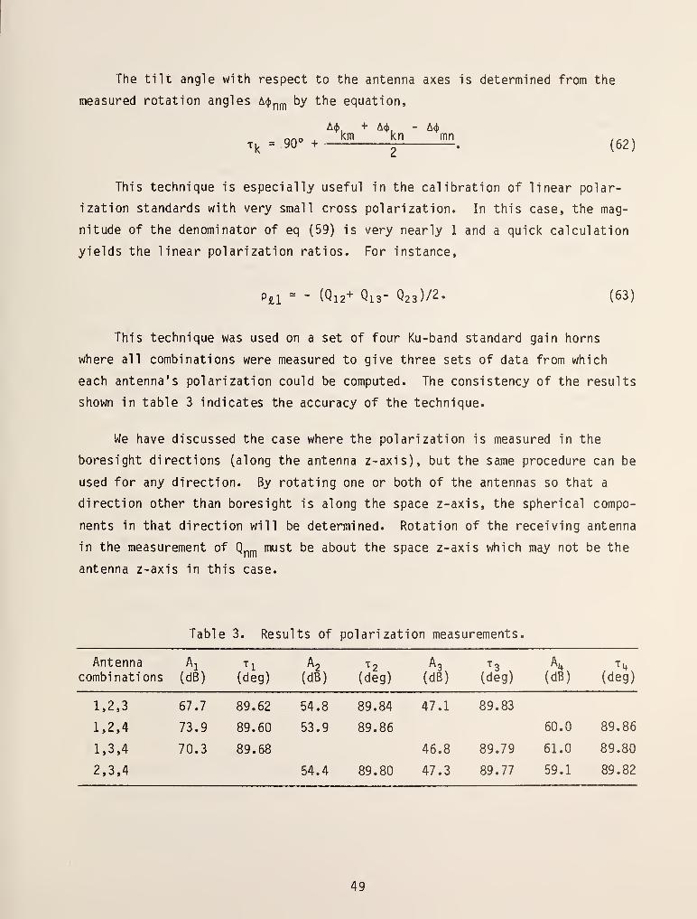
The tilt angle with respect to the antenna axes is determined from the

measured rotation angles A(|)p^ by the equation.

Ad), + Ad), - Ad)

,^=,90°.-^!! f ^. (62)

This technique is especially useful in the calibration of linear polar-

ization standards with ^Qvy small cross polarization. In this case, the mag-

nitude of the denominator of eq (59) is very nearly 1 and a quick calculation

yields the linear polarization ratios. For instance,

PU " - (Qi2+ Qi3- Q23)/2. (63)

This technique was used on a set of four Ku-band standard gain horns

where all combinations were measured to give three sets of data from which

each antenna's polarization could be computed. The consistency of the results

shown in table 3 indicates the accuracy of the technique.

We have discussed the case where the polarization is measured in the

boresight directions (along the antenna z-axis), but the same procedure can be

used for any direction. By rotating one or both of the antennas so that a

direction other than boresight is along the space z-axis, the spherical compo-

nents in that direction will be determined. Rotation of the receiving antenna

in the measurement ofQ^^^^

must be about the space z-axis which may not be the

antenna z-axis in this case.

Table 3. Results of polarization measurements.

Antennacombinations

Ai(dB) (deg)

A2

(dB)

^2

(deg)

A3

(dB)

"^3

(deg)

A^

(dB)

"^4

(deg)

1,2,3 67.7 89.62 54.8 89.84 47.1 89.83

1,2,4 73.9 89.60 53.9 89.86 60.0 89.86

1,3,4 70.3 89.68 46.8 89.79 61.0 89.80

2,3,4 54.4 89.80 47.3 89.77 59.1 89.82

49

The accuracy of the results are primarily dependent on the measurement of

the magnitude of the Q's. If care is taken to average the effect of multipath

by moving one antenna a small distance in the z-di recti on, the errors in A are

on the order of ± 0.05 dB/dB of axial ratio, and about ± 0.2 deg in t.

8. Swept Frequency Measurement Techniques

Careful measurements of gain versus frequency of standard gain horns

exhibit small periodic amplitude oscillations of the order of 0.1 to 0.2 dB

superimposed on a smooth monotonic gain function. These oscillations are

attributed to multiple reflections between the mouth and throat of the horn

[7]. For highest accuracy, the gain must be determined at closely spaced fre-

quencies and swept frequency techniques may be used. The parameters are meas-

ured as a function of frequency and the values are adjusted at specific fre-

quencies to agree with the more accurate but time consuming extrapolation

measurements. The resulting gains as a function of frequency are fully cor-

rected for mismatch, near-zone effects and multiple reflections between

antennas. The accuracy obtainable over the band will typically be of the

order of ±0.15 dB.

As implied earlier, the extrapolation method is used as the basis for

accurate swept (stepped) frequency gain calibrations (fig. 16). To accomplish

this, fixed frequency extrapolation measurements are usually performed at the

end and mid-points of a waveguide band. Next, swept measurements of the per-

tinent reflection coefficients (both amplitude and phase) are taken looking

into (1) generator port, (2) transmitting antenna, (3) receiving antenna, and

(4) load port. Examples are given in figures 17 through 20. From these

values, the mismatch correction is calculated as a function of frequency

(fig. 21).

The next step in taking swept frequency measurements is to determine the

z-di stance at which the measurements will be taken. This is done by examining

the extrapolation data and determining the distance where the insertion loss

is approximately -10 to -12 dB. This usually assures that the distance is

about 1 to 2 a^/x, which is sufficient for currently specified error uncer-

tainties. This distance also ensures that there is a measurable signal across

the band. It is at this distance that the near-zone correction is obtained

50

+->

c(UE0)i.

fOQiE>>

ca>

cr

f->Q.<U3:to

•^

0)

51

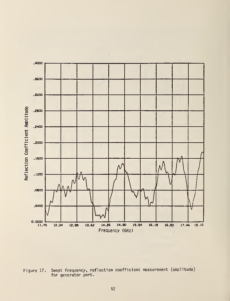
.40C»

.3600

.3200

C3"5 .2800

« .24004-<

c

L>

j: .2000

o(-}

co

0)

leoo

.1200

.0600

.0400

0.0000

L A f

1 A r" s AA,1^A a/ \ / \, n /

n1yv

\1, /

vV VJ U V

11.70 12.34 12.96 13.62 14.26 14.90 15.54 16.18 16.82 17.46 IB. 10

Frequency (GHz)

Figure 17. Swept frequency, reflection coefficient measurement (amplitude)

for generator port.

52

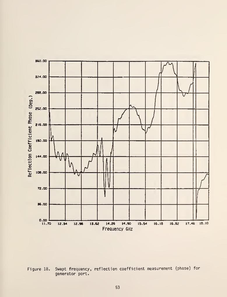
v>o

S60.00

324.00

288.00

252.00

216.00

IT 180.00I*-

o;o

% 144.00

4-<

u

72.00

96.00

0.00

^ 1

j

\ \

f

'V

/\ I

V 1

si V^

V\A A rJ\l \wv\

V/vv

V/

1

1

11.70 12. S4 12.96 iS.62 14.26 14.90 15.54 16.18 16.82 17.46 IB. 10

Frequency GHz

Figure 18. Swept frequency, reflection coefficient measurement (phase) for

generator port.

53

.4000

.S600

.S2X

.2800

*^ .2400

a>

uIt- .2000

Ooco .1600^^4-*

uo^mmu- .12000)

.0600

.0400

0.000011.70 12. S4 12.96 1S.62 14.26 14.90 15.54

Frequency (GHz)

16.18 16.82 ir.46 18. IC

Figure 19. Swept frequency, reflection coefficient measurement (amplitude)

for a long pyramidal horn.

54

Deg.

S60.00

324.C»

2SB.00

fl)252.00

O

4-« 216.00Ci««^

unm

t(-

180.00O

c=o4-«

144.

W

106.00

72.00

36.00

0.0011.70 12.54 12.96 13.62 14.26 14.90 15. &4 16.18 16.82 17.46 18. :0

Frequency (GHz)

Figure 20. Swept frequency, reflection coefficient measurement (phase) for a

long pyramidal horn.

55

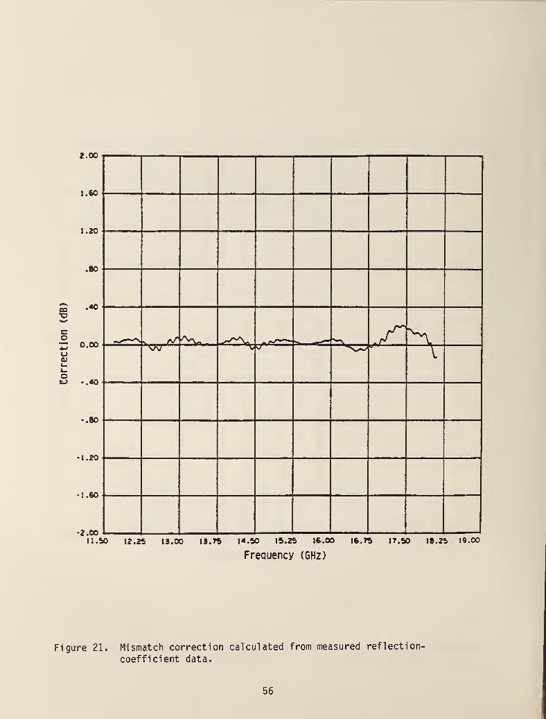
e

2.00

1.60

i.20

.80

.40

o4-«

0.00uVk.1-oo -.40

-.80

1.20

1.60

-2.00

rJ'A^ ^^^ •/^/^-^ ^-\ ./• "A^Vs/'^ ^ 0**=

\

11.50 12.25 IS.00 1S.T5 1«.50 15.25 16.00 I6.T5 17.50 18.25 19.00

Frequency (GHz)

Figure 21. Mismatch correction calculated from measured reflection-

coefficient data.

56

from the fixed-frequency extrapolation measurements (fig. 22). The receiving

system is then initialized by requiring that the receiver is operating in its

linear range and that the analog-to-digital amplitude meter is within its

operating range (0 to -20 dB). The computer is then programmed to step

(sweep) the signal source from f^^p to f^^^ ""^ steps small enough to assure

that small variations in antenna gain are measured. Usually, f^^^ and f^^^^

are chosen to be the lowest and highest frequencies at which extrapolation

range gain measurements at fixed frequencies were taken. Frequency and ampli-

tude data are then recorded (fig. 23).

The towers are then brought together and a generator-load connection is

made. A recorded offset has been inserted on the precision rotary vane

attenuator (RVA) to reduce the power level and again insure proper receiver

system operation. Frequency and amplitude data for this hookup are then

recorded (fig. 24).

After this procedure is checked out, the measurement is redone at least

twice for each pair of antennas. The sequence becomes first to measure the

generator-load connection, followed by reinstalling the horns, removing the

RVA offset, moving the towers to the appropriate distance and then recording

the frequency and amplitude measurements.

We now have sufficient information to determine the gain as a function of

frequency, fully corrected for mismatch, near zone, and multiple reflection

effects between antennas. Figure 25 shows a typical insertion loss result

including mismatch and near-zone corrections for a pair of Ku band horns.

This insertion loss is the difference between the generator-load reference

curve and the insertion loss curve with the antennas in place, both mentioned

above. The high frequency oscillations are due to multiple reflections

between the antennas. The effects can be either averaged out or filtered out

as shown in figure 26. The average gain for the pair of antennas is then

determined as shown in figure 27. After processing the average gains obtained

from the measurement of the three antenna pairs, the final gain values for the

standard gain horns are determined. Some final results are shown in fig-

ures 28 and 29. The oscillations about the nominal values are approximately

±0.04 dB, ±0.1 dB, respectively, and are due to mismatches or multiple reflec-

tions at the throat and aperture of the horns.

57

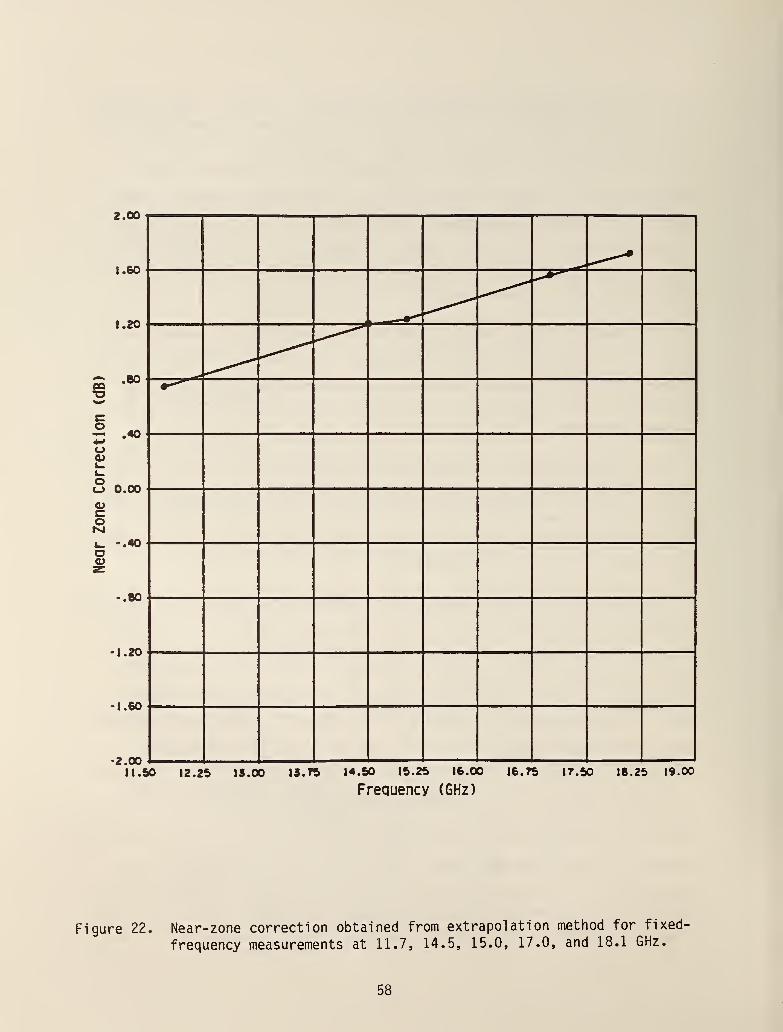
1 tw\^^

1 .«t>

t 9r\

^^^^2cB 404-»

U

(_> 0.00

ac

4_ -••Oo

-.80

-1.20

•i.60

11.50 12.25 IS.OO 15.75 I«.50 15.25 16.00 16.75 17.50 18.25 1900

Frequency (GHz)

Figure 22. Near-zone correction obtained from extrapolation method for fixed-

frequency measurements at 11.7, 14.5, 15.0, 17.0, and 18.1 GHz.

58

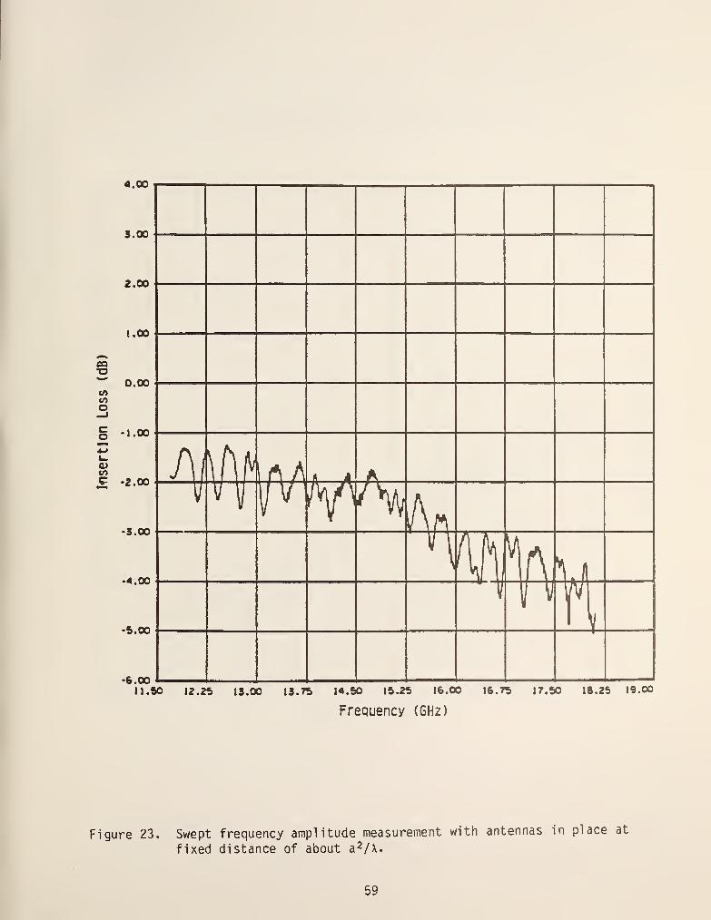
t/i

tno

i/i

4.00

5.00

2.00

1.00

0.00

1.00

^ -2.00

•3.00

•4.00

-5.00

-6.0011.50 12.25 IS.00 13.75 14.50 15.25 16.00 16,75 17,50 18.25 19.00

Frequency (GHz)

Figure 23. Swept frequency amplitude measurement with antennas in place at

fixed distance of about a^/x.

59

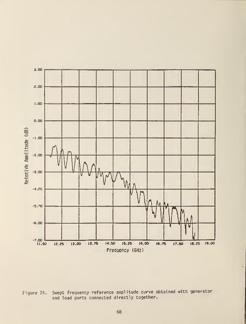
3.00

2.00

1.00

0.00

oa•o^^

-J.0003"O34-*^mm^Haf

§•2.00

<>4-* -5.00oa

•4.0G

-5. no

-6.00

•7.00II.SO 12.25 IS.OO IS. 75 14.50 15.25 16.00 16.75

Frequency (GHz)

17.50 18.25 19.00

Figure 24. Swept frequency reference amplitude curve obtained with generator

and load ports connected directly together.

60

9.00

B.OO

r.oo

6.00

e 5.00

cnO

u

o

4.00

3.00

2.00

1.00

0.00

1.00

A/v^A*.A^^

^^,^^ r **'^

J- f^^^j^

rJV

11.50 12.25 13.00 13.75 14.50 15.25 16.00

Frequency (GHz)

16.75 17.50 18.25 19.00

Figure 25. Insertion loss including mismatch and near-zone corrections. Thisis the difference between the reference curve and amplitude curvewith antennas in place. The high-frequency oscillations are due

to multiple reflections between the antennas.

61

9.CX>

8.00

7.00

«>« 6.00CQ•o"^

Vitoo 5.00,J

c;ow4

1- 4.00O)COc"-*

"S J.OO4-'

-oVk.L.O 2.00

1.00

0.00

I.OO

_.

.

t ^^ t^J\f/-^;^AM

^.r^^ "\fV-V

!^fv^^^

\f\j**

11.70 12.34 12.98 13.62 14.26 14.90 15.54 16.18 16.82 17.46 18.10

Frequency (GHz)

Figure 26. Insertion loss with multiple reflections averaged out>

62

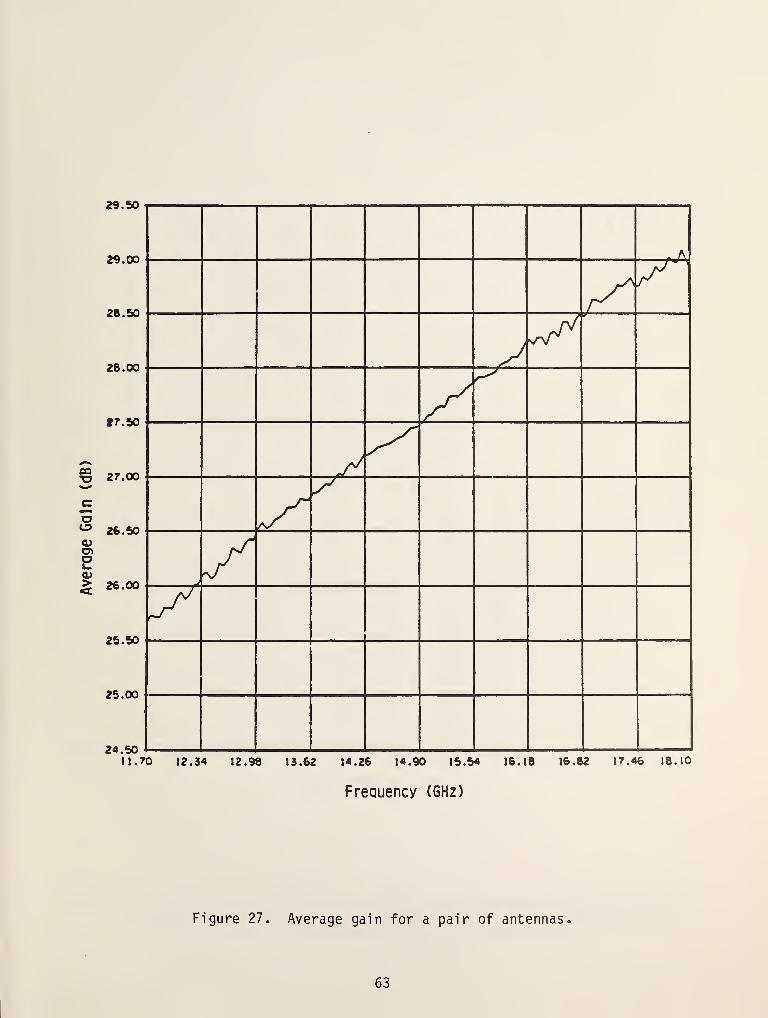
29.50

29.00

28.50

28.00

17.50

© 27.00

O^ 26.50a>

o

> 26.00

25.50

25.00

24.50

r A

r^/

y^r^

.^

Xy

/^'

11.70 12.34 12.98 13.62 14.26 14.90 15.54 16.18 16.82 17.46 IB.IO

Frequency (GHz)

Figure 27. Average gain for a pair of antennas

63

29.00

26.60

26.20

27.60

^5

27.40

o 27.00

Qi*•>

=326.60

26.20

25.60

25.40

25.00

^ <

//

J

^/

fj

//

//t

10.00 11.00 12.00 IS.00 14.00 15.00 16.00 17.00 16.00 19.00 20.00

Frequency (GHz)

Figure 28. Final gain values for a long Ku-band horn. The oscillations aboutthe nominal values are approximately ±0.04 dB and are due to

mismatches at the throat and aperture of the horn.

64

».oo

24.80

24.60

24.40

ttT3

24.20

C

s 24.00

0)

3

g2s.eo

2S.60

23.40

23.20

23.0010.00 11.00 12.00 13.00 14.00 15.00 16.00 17.00 18.00 19.00 20.00

Frequency (GHz)

Figure 29. Final gain values for a standard gain horn. The oscillationsabout the nominal values are approximately ±0.1 dB and are due to

mismatches at the throat and aperture of the horn.

65

23.0

22.5

£QO

<22.0

21.5

21.0

THEORETICAL GAINMEASURED GAIN

8 9 10 11 12 13

FREQUENCY (GHZ)

Figure 30. Comparison between theoretical gain and gain measured by theswept-frequency technique for an X-band pyramidal horn. Gainvalues indicated by the * were obtained by the extrapolationmethod.

66

As another example, figure 30 illustrates a comparison between a theo-

retically obtained gain curve for an X-band pyramidal horn as predicted by

theory [6] and data obtained using the three-antenna method applied to swept

frequency data.

9. Summary

The extrapolation range measurement technique has been described for

determining the power gain and polarization of antennas at reduced distances.

It is used extensively by the National Bureau of Standards, Boulder, Colorado

to calibrate antenna gain standards for industry and other agencies. A modi-

fication in the approach that significantly increases the accuracy of the

polarization parameters has also been described and should be of particular

interest to the reader.

Tv;o extensions of the extrapolation method have also been presented. The

first extension applies to swept frequency measurements where it has been

demonstrated that accuracies over an entire band of frequencies can be

achieved typically to within ±0.15 dB. Swept frequency measurements continue

to be of interest to the measurement community as they can determine whether

"holes" exist in an antenna's frequency response.

The second extension of the extrapolation method given as an appendix

corrects for the effects of ground reflections in absolute gain measurements.

This is particularly significant for broadbeam antennas such as those encoun-

tered below 1 GHz, where ground reflections may produce unwanted oscillations

in the ampl itude-versus-distance data.

In summary, the main purpose of this technical note is to describe the

extrapolation measurement method, its improvements and its extensions, and its

errors in detail. Through this exposition, it is hoped that managers, engi-

neers, and technicians involved in antenna measurements will understand the

deliberate steps necessary to ensure calibrations of the highest accuracy.

67

10. References

[I] Kerns, D. M. Plane-v/ave scattering-matrix theory of antennas andantenna-antenna interactions. Nat. Bur. Stand. (U.S.) Monogr. 162; 1981June.

[2] Leach, W. M., Jr.; Paris, D. T. Probe compensated near-field measure-ments on a cylinder. IEEE Trans. Antennas Propagat. AP-21: 435-445;1973 July.

[3] Yaghjian, A. D. Near-field antenna measurements on a cylindrical sur-face: A source scattering-matrix formulation. Nat. Bur. Stand. (U.S.)Tech. Note 696; 1977 September.

[4] Jensen, F. Electromagnetic near-field far-field correlations. PhD.Dissertation, the Technical University of Denmark, Lyngby; 1970 June.

[5] Wacker, P. F. Non-planar near-field measurements: Spherical scanning.Nat. Bur. Stand. NBSIR 75-809; 1975 June.

[6] Monk, A. D. Pyramidal horn gain prediction and finite range correction.The Marconi Review. XLIV: 225-243; 1981 Fourth Quarter.

[7] Jull, E. V. Errors in the predicted gain of pyramidal horns. IEEETrans. Antennas Propagat. AP-21: 14-18; 1973 January.

[8] Hamid, M. A. K. Diffraction by a conical horn. IEEE Trans. AntennaPropagat. AP-16: 520-528; 1968 September.

[9] Chu, T. S.; Legg, W. E. Gain of corrugated conical horns. IEEE Trans.Antennas Propagat. AP-30: 698-703; 1982 July.

[10] Bowman, R. R. Field strength above 1 GHz; measurement procedures forstandard antennas. Proc. IEEE 55: 921-990; June 1967.

[II] Wacker, P. F. Theory and numerical techniques for accurate extrapola-tion of near-zone antenna and scattering measurements. Nat. Bur. Stand.(U.S.) unpublished report; 1972 April.

[12] Newell, A. C; Kerns, D. M. Determination of both polarization andpower gain of antennas by a generalized 3-antenna measurement method.Electron. Lett. 7: 68-70; 1971 February 11.

[13] Newell, A. C; Baird, R. C; Wacker, P. F. Accurate measurement ofantenna gain and polarization at reduced distances by an extrapolationtechnique. IEEE Trans. Antennas Propagat. AP-21(4): 418-431; 1973 July.

[14] Kerns, D. M. Definitions of v, i, Z, Y, a, b, r, and S. Proc. IEEE.55: 892-900; 1967.

[15] Kerns, D. M.; Dayhoff, E. S. Theory of diffraction in microwave inter-ferometry. Nat. Bur. Stand. (U.S.) J. Res. 64B: 1-13; 1960 January-March.

68

[16] Beatty, R. W. Discussion of errors in gain measurements of standardelectromagnetic horns. Nat. Bur. Stand. (U.S.) Tech. Note 351; 1967March.

[17] Mollis, J. S.; Lyon, T. J.; Clayton, L. Microwave antenna measurements.Atlanta, GA: Scientific Atlanta, Inc. 1970 July. p. 10-1 through 10-38.

[18] Hollis, J. S.; Lyon, T. J.; Clayton, L. Microwave antenna measurements.Atlanta, GA: Scientific Atlanta, Inc. 1970 July. p. 3-39 through 3-46.

[19] Anson, W. J. A guide to the use of the modified reflectometer techniqueof VSWR measurements. Nat. Bur. Stand. (U.S.) J. Res. Eng. Instr.65C(4): 217-222; 1961 October-December.

[20] Kerns, D. M.; Beatty, R. W. Basic theory of waveguide junctions andintroductory microwave network analysis. Oxford, England: PergamonPress; 1967.

[21] Natrella, M. G. Experimental statistics. Nat. Bur. Stand. (U.S.):Handb. 91, 1-8; 1963.

[22] Kendall, M. G.; Stuart, A. The advanced theory of statistics. Vol. 2,

Inference and relationship. New York: Hafner, 86; 1967.

[23] Wait, D. F.; Daywitt, W. C; Kanda, M.; Miller, C. K. S. A study of themeasurement of G/T using Cassiopeia A. Nat. Bur. Stand. (U.S.) NBSIR74-382; 1974 October.

[24] Kanda, M. Accuracy considerations in the measurement of the power gainof a large microwave antenna. Succinct papers, IEEE Trans. AntennasPropag.; 1975 May.

[25] Ludwig, A.; Hardy, J.; Norman, R. Gain calibration of a horn antennausing pattern integration. Jet Propulsion Lab., Pasadena, CA, Tech.Report 32-1572; 1972 October.

[26] Chu, T. S.; Semplak, R. A. Gain of electromagnetic horns. Bell Syst.Tech. J. pp 527-537; 1965 March.

[27] Ippolito, L. J., Jr. Radiowave propagation in satellite communications.New York: Van Nostrand Reinhold Co.; 1986.

[28] Joy, E. B.; Paris, D. T. A practical method for measuring the complexpolarization ratio of arbitrary antennas. IEEE Trans. Antennas Propag.AP-21: 432-435; 1973 July.

[29] Newell, A. C. Improved polarization measurements using a modified threeantenna technique. AP-S Int. Symp. Digest: 337-340; 1975 June.

69

Appendix A.

Extension of Extrapolation Technique to Correctfor Effects of Ground Reflections

A-1

88 IEEE TRANSACTIONS ON INSTRUMENTATION AND MEASUREMENT. VOL IM-32, NO I, MARCH 1983

Antenna Gain Measurements by an ExtendedVersion of the NBS Extrapolation Method

ANDREW G. REPJAR, SENIOR MEMBER, IEEE, ALLEN C. NEWELL, MEMBER, IEEE,

AND RAMON C. BAIRD, SENIOR MEMBER, IEEE

Abstract—A General Extrapolation Technique which corrects for

the effects of ground reflections in absolute gain measurements is

described. It utilizes the Extrapolation Method developed at NBSwhich, in its present form, utilizes only amplitude versus distance data.

However, for broadbeam antennas such as those encountered below

1 GHz, ground reflections may produce unwanted oscillations in the

amplitude versus distance data. Hence the data are not amenable to

the curve-ntting procedure of the Extrapolation Method. This problem

can be overcome by including phase versus distance information to

reduce the effects of ground reflections.

INTRODUCTION

ASPECIFIC OBJECTIVE of the Antenna Systems

. Metrology Group at NBS is to develop the required

techniques and standards for accurately determining antenna

characteristics. One existing NBS measurement service is the

accurate calibration of transfer standard antennas (on-axis

gain and polarization) by the Extrapolation Method. Thetheoretical basis of this method was developed by Wacker [ 1

]

and its application to accurate antenna measurements has been

described briefly by Newell and Kerns [2] and more fully, in

an experimentally oriented paper, by Newell et al. [3]. Themethod utilizes a generalized three-antenna approach which

does not require quantitative a priori knowledge of the an-

tennas.

The main advantages of the Extrapolation Method, which

presently utilizes amplitude versus distance data only, are its

accuracy and generality, and there is essentially no upper

frequency limit. It can, in principle, be applied to any type of

antenna although some directivity is desirable to reduce

multipath interference. Above 1 GHz, uncertainties between

±0.08 and ±0.10 dB in gain are achieved routinely. Themaximum gain values that can be measured depend on the

range dimensions since a maximum separation of approxi-

mately 2D-/X is desirable. With the present NBS facilities,

the maximum gain ranges from about 45 dB at 75 GHz downto about 25dBat 1 GHz.

At frequencies below 1 GHz and for the purposes of this

paper, in the V H F- U H F region, a transfer standard is often

broadbeam and produces ground reflections which cause os-

cillations in the amplitude data as a function of distance. These

oscillations have longer periods than those due to the multiple

reflections between antennas which are routinely averaged out

Manuscript received August 19, 1982.

The authors are with the Antenna Systems Metrology Section, Electro-

magnetic Fields Division. National Bureau of Standards. Boulder. CO80303

RADIATION ABSORBING MATERIAL

TRANSMITTER

'A ^

Fig. 1 . Schematic diagram showing the NBS indoor extrapolation range

modified to function as a scaled model of the larger outdoor range.

in the Extrapolation Method. For this reason, below 1 GHzand for gains less than about 1 5 dB, the antenna might not be

calibratable by the usual Extrapolation Method which uses

a curve-fitting procedure to determine gain. The purpose of

this paper is to demonstrate that by utilizing both amplitude

and phase data as a function of distance, one can obtain an

amplitude versus distance curve which is corrected for the

effects of ground reflections. This curve can then be processed

by the Extrapolation Method to determine gain.

Discussion of Measurement Procedure

Recently at NBS, it was determined that a VHF-UHFscalar horn can be designed to meet the requirements of a

transfer standard for 240-400 MHz [4]. This fact was dem-

onstrated by designing and constructing a C-band model of

the VH F-UH F antenna .md extensively measuring the critical

performance parameters and comparing them with theoretical

results. The expected calibration accuracy of the VHF-UHFhorn was then determined by performing measurements of the

scaled model on the NBS indoor extrapolation range. Mea-

surements were conducted both with and without ground re-

flections so that we could determine how well we could correct

for the multipath effects in our calibration technique. Ulti-

mately, the full-scale horn will be measured on the NBS out-

door extrapolation range. Fig. I is an illustration of how we can

use the scaled model horn on the indoor range to simulate the

situation that will exist at 240-400 MHz on the outdoor

range.

Extrapolation Method

The first step in the measurement process is to connect the

generator and load ports together to obtain a reference signal.

The antennas are then installed and the received signal is re-

U.S. Government work not protected by U.S. copyright

A-2

REPJAR el al : ANTENNA GAIN MEASUREMENTS BY NBS EXTRAPOLATION 89

.e 1.0

SEPARATION DISTANCE (m)

Fig. 2. Extrapolation data for scalar horn showing the insertion loss

plotted as a function of separation distance (meters).

"1\ 1 1 1 1 1 T

LEAST SQUARE FIT TO DATA\-^ MEASURED DATA io

~

-DIFFERENCE AXIS

'-DIFFERENCE X 60

D = ANTENNA DIAMETER

1.0 2.0

RECIPROCAL NORMALIZED DISTANCE, 5ZA (m)

Fig. 3. Measured data without ground plane, four-term polynomial fit,

and differences for scalar horn.

corded as a function of the separation distance. Fig. 2 displays

some typical data for the case where no ground reflections are

present. The oscillations are due to multiple reflections between

the antennas. In the curve-fitting process to determine gain,

the effects of these multiple transits are eliminated by locally

averaging the relative insertion-loss values. The averaged curve

is then fitted with a polynomial in I Id (ordinarily, four or five

terms will suffice). This procedure determines the coefficient,

/4oo. of the \ jd term of the series (see [3], eq (27)] which de-

termines the gain of the antenna under test. With the artificial

ground plane removed and, hence, with no ground refiections

present, the results obtained by the curve-fitting procedure are

given in Fig. 3, which shows the averaged curve obtained from

the measured data for the scalar horn and the curve obtained

by fitting with a four-term polynomial. The greatly magnified

differences between the measured and fitted curve qualitatively

indicate the goodness of fit. The absolute gain of this horn was

determined to be 13.32 dB at 4.0 GHz, which simulates 240

MHz in the VHF-UHF range. It should be noted that the

abscissa in Fig. 3, and subsequently in Figs. 4 and 6, is the in-

verse of the normalized separation distance, a natural meansof analyzing curve fitting with a polynomial in 1 /d.

Analysis

With the artificial ground plane in place, the averaged curve,

i.e., the curve obtained after applying the local averaging

process discussed above, as a function of antenna separation

"1 11 r 1 1 1 r

LEAST SQUARE FIT TO DATAH-l MEASURED DATA

1.0

RECIPROCAL NORMALIZED DISTANCE. dVA

Fig. 4. Measured data with ground plane, four-term polynomial fit, anddifferences for scalar horn.

is given in Fig. 4. Note the region of oscillatory behavior due

to ground reflections. Fitting this curve with a four-term

polynomial in 1 jd, which is also shown in Fig. 4, results in a

calculated gain of 14.29 dB, 0.97 dB higher than its calibrated

value obtained without the ground plane! In addition, it is ev-

ident from this figure that the differences between the averaged

curve and the fitted curve are pronounced.

Denoting 0, as the measured phase and (pj as the phase of

the direct wave, one can see that when the ground plane is re-

moved, i.e., no ground effects present, the measured phase

minus the phase of the direct, wave should be zero plus an ar-

bitrary constant in the far field. This is important in our

analysis because the only assumption made in obtaining an

amplitude versus distance plot that is free of multipath effects

is that the direct wave phase can be represented in the far field

as

(pd = 360 d/X degrees (1)

where d is the separation distance and X is the wavelength.

Using a laser interferometer to accurately measure the

separation distance, the phase was measured without the

ground plane to test the above assumption. (Since ( 1 ) is being

used to calculate the phase of the direct wave, the measured

separation distance must be accurate to about 1/360 of a

wavelength. For this reason, at C-band, a laser interferometer

was used to measure the separation distances. For measure-

ments of the full-scale UHF-VHF horn, other means may be

adequate.) The dashed line in Fig. 5 shows the results, dem-

onstrating that for large distances, 0, - (pd is in fact extremely

close to being constant. It should be noted that where the

separation d-stance is small, the variation of 0, — 0<y is due to

the near-zone effect, i.e., the antennas are still in the near field

of each other. (A correction for this effect is routinely obtained

in the standard extrapolation method.)

An analysis of the interaction between the direct wave and

the ground wave shows that at the local peaks of the 0, — 0^

curve

p = -L^ = sin(0, -0^) (2)

where|K^| and

| K/| ^re the amplitudes of the ground and

direct waves, respectively. In addition, it can be shown that

A-3

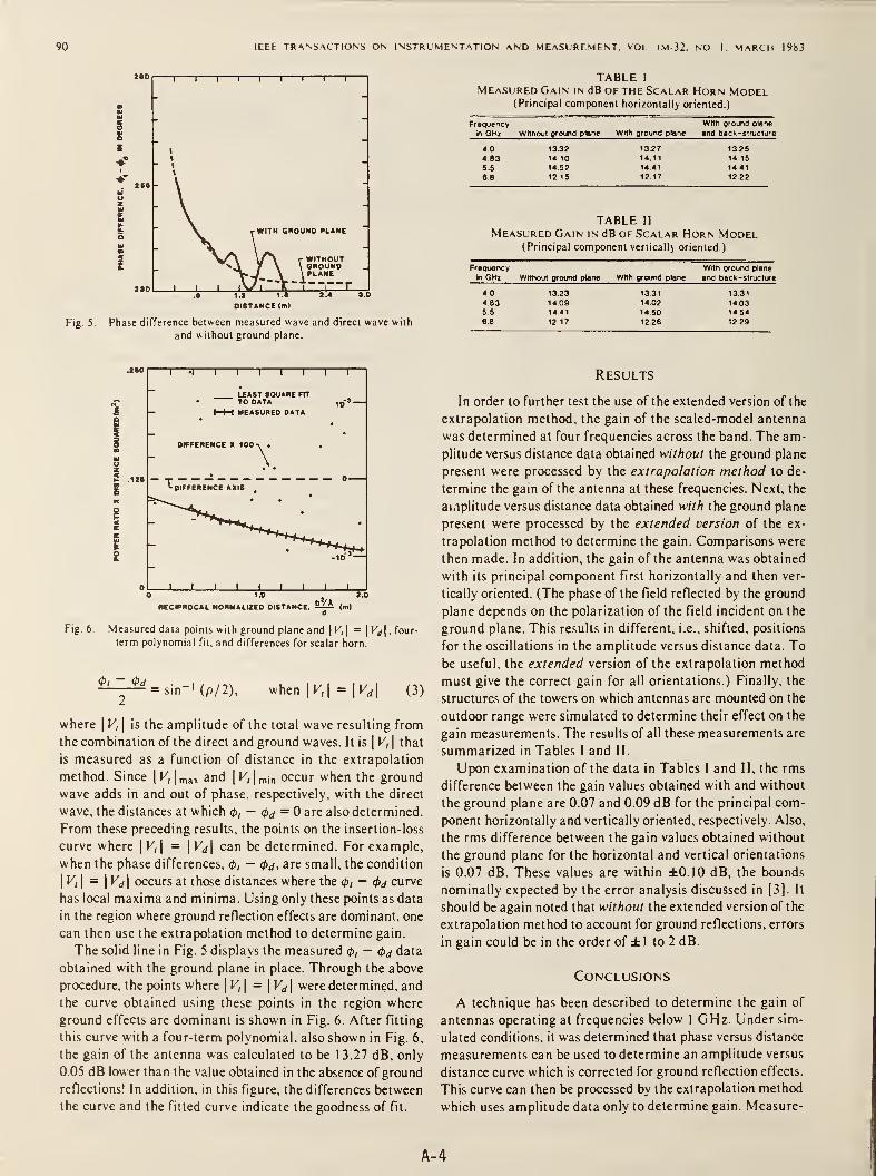
90 IEEE TRANSACTIONS ON INSTRUMENTATION AND MEASUREMENT, VOL IM-32. NO 1, MARCH 1983

Z«D

-

-I— 1 I 1 1 1 I 1 1

-

- -

- -

- 1

1

\

-

t»5

-

\

\k _

rWITH GMOUND »L*NE

-

190

-

1 1 ^ \/\ r^'TMOUT7 \ \ GROUND

/rA4--"-r-

.e 1.2 i.a i.* ».o

DISTANCE (m)

Fig. 5. Phase difference between measured wave and direct wave with

and without ground plane.

TABLE I

Measured Gain in dB of the Scalar Horn Model(Principal component horizontally oriented.)

Fre»jency With grouna plane

in GHz WIthoul grouna plane With jround plane •nd l)ack-structure

40 13.32 13.27 1325483 14 10 14.11 14 15

5.5 1452 14.41 1441e.8 12.15 12.17 12 22

TABLE MMeasured Gain in dB of Scalar Horn Model

(Principal component vertically oriented.)

Frequency Wrth ground plane

^GHz WIthoul ground ptone With ground plane •nd back -structure

4.0 1323 13.31 13.31

4.83 1409 1402 14.035.5 1441 1450 14.54

86 1217 12.26 1229

E

1 •! 1 1 1 1 1 1 1

LEAST SQUARE FITTO DATA 10-'—

- 1-4-1 MEASURED DATA

_ .

DIFFERENCE X 100 -\ . ,

\.

^DIFFERENCE AXIS .

— 0.^

^^^^^^^KU^,^

- "^ ' ^*«t,j^•

.

'^~*~*

-io'—

I 1 1 1 1 1 1 1 1

1.0 »oRECIPnOCAL NORMALIZED DISTANCE, DVA

Fig. 6. Measured data points with ground plane andIK, I = 11^^!, four-

term polynomial fit, and differences for scalar horn.

4>i — 4>d = sin-'(p/2), when|I/,| =|K<,| (3)

where \V,\ is the amplitude of the total wave resulting from

the combination of the direct and ground waves. It is|K,

|that

is measured as a function of distance in the extrapolation

method. Since|V,

\ max and|V,

\ „,(„ occur when the ground

wave adds in and out of phase, respectively, with the direct

wave, the distances at which 4>, — cp^ = are also determined.

From these preceding results, the points on the insertion-loss

curve where \V,\ = \Vj\ can be determined. For example,

when the phase differences, (p, — 4>d, are small, the condition

\y,\ = \Vd\ occurs at those distances where the (t>,—

(t>d curve

has local maxima and minima. Using only these pxjints as data

in the region where ground reflection effects are dominant, one

can then use the extrapolation method to determine gain.

The solid line in Fig. 5 displays the measured (p, — 4>d data

obtained with the ground plane in place. Through the above

procedure, the points where \V,\ =|K^| were determined, and

the curve obtained using these points in the region where

ground effects are dominant is shown in Fig. 6. After fitting

this curve with a four-term polynomial, also shown in Fig. 6,

the gain of the antenna was calculated to be 1 3.27 dB, only

0.05 dB lower than the value obtained in the absence of ground

reflections! In addition, in this figure, the differences between

the curve and the filled curve indicate the goodness of fit.

Results

In order to further test the use of the extended version of the

extrapolation method, the gain of the scaled-model antenna

was determined at four frequencies across the band. The am-

plitude versus distance data obtained without the ground plane

present were processed by the extrapolation method to de-

termine the gain of the antenna at these frequencies. Next, the

ai.iplitude versus distance data obtained with the ground plane

present were processed by the extended version of the ex-

trapolation method to determine the gain. Comparisons were

then made. In addition, the gain of the antenna was obtained

with its principal component first horizontally and then ver-

tically oriented. (The phase of the field refiected by the ground

plane depends on the polarization of the field incident on the

ground plane. This results in different, i.e., shifted, positions

for the oscillations in the amplitude versus distance data. To

be useful, the extended version of the extrapolation method

must give the correct gain for all orientations.) Finally, the

structures of the towers on which antennas are mounted on the

outdoor range were simulated to determine their effect on the

gain measurements. The results of all these measurements are

summarized in Tables I and II.

Upon examination of the data in Tables I and II, the rms

difference between the gain values obtained with and without

the ground plane are 0.07 and 0.09 dB for the principal com-

ponent horizontally and vertically oriented, respectively. Also,

the rms difference between the gain values obtained without

the ground plane for the horizontal and vertical orientations

is 0.07 dB. These values are within ±0.10 dB, the bounds

nominally expected by the error analysis discussed in [3]. It

should be again noted that without the extended version of the

extrapolation method to account for ground reflections, errors

in gain could be in the order of ± 1 to 2 dB.

Conclusions

A technique has been described to determine the gain of

antennas operating at frequencies below 1 GHz. Under sim-

ulated conditions, it was determined that phase versus distance

measurements can be used to determine an amplitude versus

distance curve which is corrected for ground refiection effects.

This curve can then be processed by the extrapolation method

which uses amplitude data only to determine gain. Measure-

A-4

IEEE TRANSACTIONS ON INSTRUMENTATION AND MEASUREMENT, VOL IM-32, NO. 1, MARCH 1983

mentson the full-scale VHF-UHF horn on the NBS outdoor

extrapolation range are planned for the future.

References

[1] p. F. Wacker, "Theory and numerical techniques for accurate extrapo-

lation of near-zone antenna and scattering measurements," NBS, Boul-

der, CO, unpublished Rep.. Apr. 1972.

[2] A. C. Newell and D. M. Kerns, "Determination of both polarization and

power gain of antennas by a generalized 3-antenna measurement meth-

od." £/mro^ Z,e»., vol. 7, pp. 68-70, Feb. II, 1971.

[3] A. C. Newell. R. C. Baird. and P. F. Wacker, "Accurate measurementof antenna gain and polarization at reduced distances by an extrapolation

technique." IEEE Trans. Antennas Propagal., vol. AP-21. no. 4. pp.

418-431, July 1973.

[4] A. J. Estin, C. F. Stubenrauch, A. G. Repjar, and A. C. Newell, "Opti-

mized wavelength-sized scalar horns as antenna radiation standards,"

IEEE Trans. Instrum. Meas., vol. IM-31, no. 1, pp. 53-56, Mar.1982.

A-

5

Appendix B.

Standard NBS Calibration Report

B-1

U.S. DEPARTMENT OF COMMERCENATIONAL BUREAU OF STANDARDS

NATIONAL ENGINEERING LABORATORYBoulder, Colorado 80303

REPORT OF CALIBRATION

STAM)ARD GAIN HORNNational Bureau of StandardsX-Band Horn, Serial No. 485

calibrated againstNational Bureau of Standards

International Comparison Standard, Serial No. 1

andNational Bureau of Standards

International Comparison Standard, Serial No. 2

Submitted by:

National Bureau of StandardsAntenna Systems Metrology Group

Boulder, Colorado 80303

The on-axis power gain and polarization parameters of the antenna were measured by a

generalized three antenna measurement technique [1]. An extrapolation measurementtechnique was used to evaluate and correct for near-zone and multipath effects in

the measured data. The two other antennas which were used in the measurement werepyramidal type horns with nominal linear polarization. The antennas were notassumed to be perfectly linearly polarized, and their actual cross polarization wasaccounted for in the measurements and calculations.

The axis of measurement was in the direction of maximum power gain for all antennas,and their 'E* field was in the horizontal direction.

The results of the measurements are summarized in the following table.

Frequency(GHz)

Power Gain(dB)

Axial Ratio(dB)

Sense ofPolarization

Tilt Angle(degrees)

ReflectionAmplitude

CoefficientPhase

(degrees)

8.0010.0012.00

21.60 ± 0.122.37 ± 0.122.78 ± 0.1

48 ± 2

44 ± 2

43 ± 2

RightRightRight

90.3 ± 0.590.1 ± 0.590.3 ± 0.5

0.0490.0430.025

105.9-59.6

-147.9

In addition to the gain measurements at the fixed frequencies, swept gainmeasurements were also obtained. The results of these measurements are shown in

figure 1

.

[1] Newell, A. C; Baird, R. C; Wacker, P. F. Accurate measurement of antenna gainand polarization at reduced distances by an extrapolation technique. IEEE

Trans. Antennas and Propagation, Vol. AP-21:418-431; 1973 July.

Page 1 of 2

Date of Calibration: July 1982

B-2

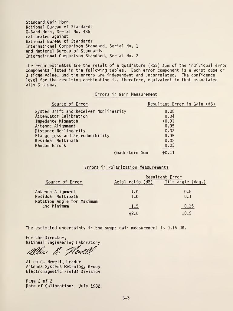
standard Gain HornNational Bureau of StandardsX-Band Horn, Serial No. 485calibrated againstNational Bureau of StandardsInternational Comparison Standard, Serial No. 1

and National Bureau of StandardsInternational Comparison Standard, Serial No. 2

The error estimates are the result of a quadrature (RSS) sum of the individual errorcomponents listed in the following tables. Each error component is a worst case or

3 Sigma value, and the errors are independent and uncorrelated. The confidencelevel for the resulting combination is, therefore, equivalent to that associatedwith 3 sigma.

Errors in Gain Measurement

Source of Error

System Drift and Receiver NonlinearityAttenuator CalibrationImpedance MismatchAntenna AlignmentDistance NonlinearityFlange Loss and ReproducibilityResidual MultipathRandom Errors

Resultant Error in Gain (dB)

0.050.04

<0.010.050.020.050.030.03

Quadrature Sum ±0.11

Errors in Polarization Measurements

Resultant ErrorSource of Error Axial ratio (dB) Tilt angle (deg.)

Antenna Alignment 1.0 0.5Residual Multipath 1.0 0.1Rotation Angle for Maximum

and Minimum 1.5 0.15

±2.0 ±0.5

The estimated uncertainty in the swept gain measurement is 0.15 dB,

For the Director,National Engineering Laboratory

Allen C. Newell, LeaderAntenna Systems Metrology GroupElectromagnetic Fields Division

Page 2 of 2

Date of Calibration: July 1982

B-3

INT. CO»i^. STD. XTR S/ll 485

2J, 00

2.?. 80

22.60

22.40

22.20

to

c 22.00

(0

21.80

21.00

21.40

21.20

21.00

/ \y

A/^/kJ

r^/

^ /

, /\ 1

V

8.00 8.40 8.80 9.20 9.60 10.00 1040 10.80 11 .-20 11.60 12.00

Frequency in GHz

Figure 1. NBS X-Band Horn, Serial No. 485.

B-4

NBS-IUA IREV. 2-6C)

U.S. DEPT. OF COMM.

BIBLIOGRAPHIC DATASHEET (See instructions)

1. PUBLICATION ORREPORT NO.

NBS/TN-13n

2. Performing Organ. Report No, 3. Publication Date

August 19884. TITLE AND SUBTITLE

Extrapolation Range Measurements for Determining Antenna Gain and Polarization

5. AUTHOR(S)

Andrew G. Repjar, Allen C. Newell, and Douglas T. Tamura

6. PERFORMING ORGANIZATION (If joint or other than NBS. see instructions)

NATIONAL BUREAU OF STANDARDSDEPARTMENT OF COMMERCEWASHINGTON, D.C. 20234

7. Contract/Grant No.

8. Type of Report & Period Covered

9. SPONSORING ORGANIZATION NAME AND COMPLETE ADDRESS (Street. City. State, ZIP)

10. SUPPLEMENTARY NOTES

[^ Document describes a computer program; SF-185, FlPS Software Summary, is attached.

11. ABSTRACT (A 200-word or less factual summary of most si gnificant information. If document includes a significantbibliography or literature survey, mention it here)

The extrapolation range measurement technique for determining the power gain and

polarization of antennas at reduced range distances is described. It is based on a

generalized three-antenna approach and does not require quantitative a priori knowl-edge of the antennas. During the past decade, it has been extensively used by theNational Bureau of Standards, Boulder, Colorado, to calibrate antenna gain standardsfor industry and other agencies within +0.1 dB. To help one understand how calibra-tions of this accuracy are achieved, the extrapolation range description includesdiscussions on the required theory, the measurement procedures, the range configura-tion and instrumentation, the errors, and some measurement examples. Recent exten-sions of the extrapolation method required for swept/stepped frequency gain calibra-tions and for corrections to reduce ground reflection effects, are also presented.

12. KEY WORDS (Six to twelve entries; alphabetical order; capitalize only proper names; and separate key words by semicolons)

antenna measurements: antenna ranges; antennas; near-field measurements; probe antennasstandard gain horns; swept frequency measurements

13. AVAILABILITY

[jj[] Unl imited

I I

For Official Distribution. Do Not Release to NTIS

fXI Order From Superintendent of Documents, U.S. Government Printing Office, Washington, D.C.20402.

1231 Order From National Technical Information Service (NTIS), Springfield, VA. 22161

14. NO. OFPRINTED PAGES

8815. Price

USCOMM-DC 6043-P80»U.S. GOVERNMENT PRINTING OFFICE: 19 8 7-0-77 6-9 23/65 298

NBSTechnical Publications

Periodical

Journal of Research—The Journal of Research of the National Bureau of Standards reports NBS research

and development in those disciplines of the physical and engineering sciences in which the Bureau is active.

These include physics, chemistry, engineering, mathematics, and computer sciences. Papers cover a broadrange of subjects, with major emphasis on measurement methodology and the basic technology underlying

standardization. Also included from time to time are survey articles on topics closely related to the Bureau's

technical and scientific programs. Issued six times a yecir.

Nonperiodkals

Monographs—Major contributions to the technical literature on various subjects related to the Bureau's scien-

tific ctnd technical activities.

Handbooks—Recommended codes of engineering and industrial practice (including safety codes) developed in

cooperation with interested industries, professional organizations, and regulatory bodies.

Special Publkalions—Include proceedings of conferences sponsored by NBS, NBS annual reports, and otherspecial publications appropriate to this grouping such as wall charts, pocket cards, £ind bibliographies.

Applied Madiematics Series—Mathematical tables, manuals, and studies of special interest to physicists,

engineers, chemists, biologists, mathematicians, computer programmers, and others engaged in scientific andtechnical work.

National Standard Reference Data Series—Provides quantitative data on the physical and chemical properties

of materials, compiled from the world's literature and critically evaluated. Developed under a worldwide pro-gram coordinated by NBS under the authority of the National Standard Data Act (Public Law 90-396).

NOTE: The Journal of Physical and Chemical Reference Data (JPCRD) is published quarterly for NBS bythe American Chemical Society (ACS) and the American Institute of Physics (AIP). Subscriptions, reprints,

and supplements are available from ACS, 1155 Sixteenth St., NW, Washington, E)C 20056.

Building Science Series—Disseminates technical information developed at the Bureau on building matericds,

components, systems, and whole structures. The series presents research results, test methods, and perfor-

mance criteria related to the structural and environmental functions and the durability and safety

characteristics of building elements and systems.

Technical Notes—Studies or reports which are complete in themselves but restrictive in their treatment of asubject. Analogous to monographs but not so comprehensive in scope or definitive in treatment of the subject

area. Often serve as a vehicle for final reports of work performed at NBS under the sponsorship of other

government agencies.

Voluntary Product Standards—Developed under procedures published by the Department of Commerce in

Part 10, Title 15, of the Code of Federal Regulations. The standards establish nationally recognized re-

quirements for products, and provide all concerned interests with a basis for common understanding of the

characteristics of the products. NBS administers this program as a supplement to the activities of the private

sector standardizing organizations.

Consumer Information Series—Practical information, based on NBS research jind experience, covering areas

of interest to the consumer. Easily understandable language and illustrations provide useful backgroundknowledge for shopping in today's technological marketplace.

Order the above NBS publications from: Superintendent of Documents, Government Printing Office,

Washington, DC 20402.

Order the following NBS publications—FIPS and NBSIR 's—from the National Technical Information Ser-

vice, Springfield, VA 22161.

Federal Information Processing Standards Publications (FIPS PUB)—Publications in this series collectively

constitute the Federal Information Processing Standards Register. The Register serves as the official source of

information in the Federal Government regarding standards issued by NBS pursuant to the Federal Property

and Administrative Services Act of 1949 as amended. Public Law 89-306 (79 Stat. 1127), and as implementedby Executive Order 1 1717 (38 FR 12315, dated May 1 1, 1973) and Part 6 of Tide 15 CFR (Code of Federal

Regulations).

NBS Interagency Reports (NBSIR)—A special series of interim or final reports on work performed by NBSfor outside sponsors (both government and non-government). In general, initial distribution is handled by the

sponsor; public distribution is by the National Technical Information Service, Springfield, VA 22161, in paper

copy or microfiche form.

U.S. Department of CommerceNational Bureau of Standards

Gaithersburg, MD 20899

Official Business

Penalty for Private Use $300