All-pay auctions—an experimental studyrady.ucsd.edu/faculty/directory/gneezy/pub/docs/all-pay-auctions.pdf · In an all-pay auction, the winner is determined according to the highest

Journal of Economic Behavior & OrganizationVol. 61 (2006) 255–275

All-pay auctions—an experimental study

Uri Gneezy a,∗, Rann Smorodinsky b,1

a The University of Chicago, Graduate School of Business, 1101 E. 58th Street, Chicago, IL 60637, USAb Faculty of Industrial Engineering and Management, Technion, Haifa 32000, Israel

Received 13 May 2004; accepted 29 September 2004Available online 3 October 2005

Abstract

This paper reports the results of a repeated all-pay auction game. The auction form used is the simplestpossible, complete information, perfect recall and common value. Our main findings are that in such anauction, over-bidding is quite drastic, and the seller’s revenue depends strongly on the number of biddersin early stages. However, after a few rounds of play, this dependence completely disappears and the seller’srevenue becomes independent of the number of participants. The results are confronted with two solutionconcepts of economic theory, the Nash-equilibrium and the symmetric Logit equilibrium.© 2005 Published by Elsevier B.V.

Keywords: All-pay; Auction; Revenue; Nash-equilibrium; Symmetric Logit equilibrium

1. Introduction

Many economic allocations are decided by competition for a prize on the basis of costlyactivities. Some well-known examples for such competitions are research and development (R&D)races, political campaigns, awarding of monopoly licenses, selling franchises, and so on. In suchcontests, participants’ efforts are quite costly, and losers are not compensated for these efforts. Tomodel such situations, in which competition involves real expenditures, or ‘rent seeking’ behavior,researchers find the all-pay auction quite appealing.

In an all-pay auction, the winner is determined according to the highest bid, and all playerspay a fraction of their bid. The logic of using the all-pay auction to model such competitionsis rooted in the assumption, commonly used in the rent seeking literature (e.g., Tullock, 1980),

∗ Corresponding author. Tel.: +1 773 834 8198.E-mail addresses: [email protected] (U. Gneezy), [email protected] (R. Smorodinsky).

1 Tel.: +972 4 8294422, fax: +972 4 829445688.

0167-2681/$ – see front matter © 2005 Published by Elsevier B.V.doi:10.1016/j.jebo.2004.09.013

256 U. Gneezy, R. Smorodinsky / J. of Economic Behavior & Org. 61 (2006) 255–275

that the probability of winning the prize is an increasing function of the efforts. An all-payauction is a limiting case in which the prize goes to the competitor who exerts the highesteffort.

One well-known phenomenon observed in empirical studies of rent seeking activities is over-dissipation. It turns out that in a variety of cases where rent-seeking behavior is exercised, totalefforts exceed the value of the prize. Krueger (1974), for example, estimates that annual welfarecosts induced by price and quantity controls in India are approximately 7% of gross nationalproduct. In Turkey, the figures are estimated as somewhat higher.

This paper reports the results of an experiment in the simplest form of an all-pay auction. First,participants’ efforts are actually equal bids in the experiment. Second, the game we use is one ofcomplete information and perfect recall,1 and the prize we use is one of common value (makingthe game symmetric). Focusing on such a reduced form of the all-pay auction is an attempt todifferentiate between patterns of behavior induced by the mechanism itself and patterns inducedby the complexity that is usually found in a ‘real-world’ environment where there is an inherentasymmetry among players and where complete information as well as perfect recall may belacking.

Our findings show that indeed the all-pay auction mechanism, without the extra ‘real world’complications, is sufficient to induce irrational (in the expected utility sense) behavior. Our mainfindings are that subjects tend to over-bid, and in most rounds of the experiment the auctioneer’srevenues (i.e., total bids) reached twice to three times the value of the prize, even after a few roundsof play. At the early stages of the game the quantitative nature of the over-bidding phenomenondepends strongly on the number of bidders participating in the auction. However, in later roundsof play, the overbidding is quite independent of the number of bidders.

We compare our results with two theoretical solution concepts, Nash equilibrium, which isbased on the assumption that players are fully rational, and the symmetric Logit equilibrium,suggested by Anderson et al. (1998), which is based on a model of bounded rationality of theplayers. It turns out that neither model can fully account for the actual behavior of our subjects inthe experiment. The Nash equilibrium, on the one hand, either fails to predict the excessive over-bidding observed or assumes that players are risk loving in an implausible manner. On the otherhand, the symmetric Logit equilibrium can explain behavior in early stages of the experiment,assuming a relatively large noise factor, but fails to account for the independence of the seller’srevenue with respect to the number of bidders at the later stages.

The study of auctions has a long tradition in experimental economics (see Kagel, 1995 for asurvey of this literature). However, the number of experimental studies of all-pay auctions is quitelimited. Most of these are designed to test Tullock’s model of efficient rent seeking. Consequently,the experiments take on a relatively complicated form, and the allocation of the prize is determinedby a lottery where each player’s probability of winning is an increasing function of his bid. To thebest of our knowledge, Millner and Pratt (1989) were the first to test this model experimentally.They found large dissipation, contradicting the Nash equilibrium forecast. However, Shogren andBaik (1991) observed behavior much closer to the Nash equilibrium prediction.

The closest work related to our experiment is that of Davis and Reilly (1998).In their paper, they report the result of an experiment of an all-pay auction with four players.

This experiment was run as part of a general scheme to understand the consequences of introducing

1 The game design is such that all the information on past play, in particular the history of bids of all individuals, is atthe players’ disposal.

U. Gneezy, R. Smorodinsky / J. of Economic Behavior & Org. 61 (2006) 255–275 257

a “rent-defending” player, in the spirit of the model in Ellingsen (1991). Participants in the Davisand Reilly experiment rotated among various treatments, one of which was an all-pay auction.Not surprisingly, Davis and Reilly also observe deviation from the Nash equilibrium prediction.In contrast, the experiment reported here takes the form of a repeated game where participantsplay the same all-pay auction, so learning is feasible. Moreover, we study the effect of the numberof auction participants on behavior. Consequently, we can relate empirical results with the Logitequilibrium forecast.

In comparison to the existing literature on all-pay auctions, our study focuses on the simplestform of an all-pay auction. The prize is allocated to the bidder with the highest bid, informationis symmetric, no rent-defending activities are introduced, and so on. The reason for this is to seewhether the over-dissipation observed results from the special form of the auction mechanismor whether other ‘obscuring’ factors, such as complication of the mechanism or asymmetricinformation, contributes to this. Furthermore, we study the impact of the number of playersparticipating in the auction (auction size). There are two reasons to study this last factor. First,since the Logit equilibrium solution predicts an increase in dissipation with the number of bidders,one should study the impact of the auction size, in order to validate this solution.2 Second, inthe spirit of the search for optimal auctions (from the seller’s perspective), motivated by theincreasing number of auction houses on the internet (e.g., OnSale at www.onsale.com and uBidat www.ubid.com), it is natural to ask whether control on the auction size can increase sellers’revenues.3

Section 2 describes the formal model (the game form) of the all-pay auction. In Section 3, wedescribe the experimental procedure. Section 4 is dedicated to the results of the model followedby an analysis, and Section 5 compares the observed results with various solution concepts of thegame. Section 6 provides a descriptive model of our results, based on a two stage Logit equilibriummodel, and Section 7 concludes.

2. The game

The game we study is a repetition of a stage game of all-pay first-price auction. In each round,all N players (called bidders) submit a bid that is a non-negative number. All bids are publiclyannounced, in an anonymous way, and the player who submitted the highest bid then gets (alsoanonymously) a prize of 1. All players pay their bid to the auctioneer whether they won the prizeor not. Note that the game described is a game of perfect recall and complete information. Also,note that the value of the prize is similar for all players.

The stage game of the all-pay auction is the following N-person game: LetR+ be each player’sstrategy space, and let Ui : RN+ → R be player i’s utility, defined by

Ui(bi) ={

1M(b)

− bi if bi ≥ bj for all j �= i

−bi otherwise,

where M(b) denotes the number of maximal elements in the set b = {b1, b2, . . . , bN} ∈RN .Note that by choosing the action 0, each player can guarantee a payoff of at least 0. Also, note

that any action bi ≥ 1 guarantees a non-positive payoff.

2 This is also suggested explicitly by Anderson et al. (1998) who advocate the use of the Logit equilibrium for modellingbehavior in all-pay auctions.

3 Obviously, this argument holds for a variety of auction procedures and not only all-pay auctions.

http://www.onsale.com/

http://www.ubid.com/


In any Nash equilibrium of this game, risk-neutral players play a mixed strategy and theexpected revenues to the seller (i.e., total bids) are equal the prize. A more detailed description ofthe Nash equilibrium solution is provided in Section 5.1.

3. Experiment procedure

The experiment was run in three distinct experimental treatments, which we entitled T4, T8,and T12. In each treatment we kept the number of participants fixed, N = 4, 8, 12 (as reflected inthe titles of the treatments). All other components of the experiments were equal for the varioustreatments.

In each treatment, we ran 5 sessions of the experiment, amounting to 15 sessions and 120participants. For the participants in the experiment, the number of players was common knowledge.The participants were undergraduate economics students, recruited in their classes.

At the beginning of the experiment, the participants were seated far away from each other andwere given an introduction to the experiment.4 Specifically, they were told that the experimentwould take about 30 min during which they would be asked to make some decisions. Also, theywere told that at the end of the experiment, they would be paid according to the decisions theythemselves made, as well as the decisions made by their fellow participants. After reading theintroduction, participants were asked to choose an envelope out of a box. Each envelope containeda number: 1, 2, . . ., N, where N denotes the number of participants (which was either 4, 8 or 12).This number was private information and was used as a participant’s “ID number”. At the endof the experiment, participants identified themselves with their ID number, so we were able topay them discretely. An extra envelope with the note “Assistant” in it determined which of thestudents would help us during the experiment. This student was paid the average payoff of allother students.5

After checking the envelopes, the instructions were distributed and were read aloud (AppendixB). After reading the instructions, participants were given a short quiz (see Appendix C) thatwas used to verify understanding of the instructions. Participants were told that failure of thequiz would mean that they could not participate in the experiment (however, in practice, none ofthe participants failed). During the experiment, accounting for the payoff was done with pointsinstead of real money. The conversion rate used was 20 points = 1 New Israeli Shekel (NIS),6 andthis was known to all participants. At the beginning of the experiment, each participant receiveda credit of 1000 points. The experiment consisted of 10 rounds. In round 1, we auctioned 100points. Each participant was asked to write his/her ID number and bid for this round on a note, tobe collected by the assistant. The bids were restricted to be between zero and the credit line.7 Theparticipant was also asked to keep track of his bids on a personal form. After collecting all the bids,the assistant took one note at a time and read aloud the ID number and the bid. This informationwas written on the blackboard. The winner in the auction (i.e., the participant who won the 100points) was the participant who submitted the highest bid. It was made clear that all participantsmust pay their bid, regardless of whether they won or lost. In case of ties, the 100 points were

4 See Appendix A of this article, which can be found in the JEBO website.5 Note that although the assistant has an incentive to help players collude, she has no means of doing so in our set-up.6 At the time of the experiment, NIS 3.7 = $ 1.7 The budget constraint imposed on the players was negligible, and in reality, no player ever reached his/her credit line.

Moreover this budget constraint has no implications on the theoretical results we cite, i.e., the Nash equilibrium and theLogit equilibrium.


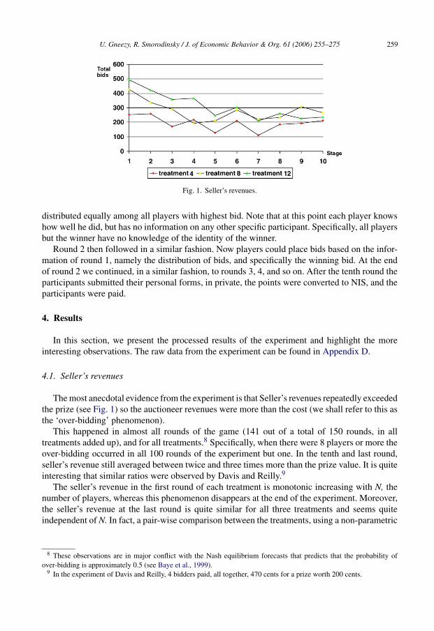
Fig. 1. Seller’s revenues.

distributed equally among all players with highest bid. Note that at this point each player knowshow well he did, but has no information on any other specific participant. Specifically, all playersbut the winner have no knowledge of the identity of the winner.

Round 2 then followed in a similar fashion. Now players could place bids based on the infor-mation of round 1, namely the distribution of bids, and specifically the winning bid. At the endof round 2 we continued, in a similar fashion, to rounds 3, 4, and so on. After the tenth round theparticipants submitted their personal forms, in private, the points were converted to NIS, and theparticipants were paid.

4. Results

In this section, we present the processed results of the experiment and highlight the moreinteresting observations. The raw data from the experiment can be found in Appendix D.

4.1. Seller’s revenues

The most anecdotal evidence from the experiment is that Seller’s revenues repeatedly exceededthe prize (see Fig. 1) so the auctioneer revenues were more than the cost (we shall refer to this asthe ‘over-bidding’ phenomenon).

This happened in almost all rounds of the game (141 out of a total of 150 rounds, in alltreatments added up), and for all treatments.8 Specifically, when there were 8 players or more theover-bidding occurred in all 100 rounds of the experiment but one. In the tenth and last round,seller’s revenue still averaged between twice and three times more than the prize value. It is quiteinteresting that similar ratios were observed by Davis and Reilly.9

The seller’s revenue in the first round of each treatment is monotonic increasing with N, thenumber of players, whereas this phenomenon disappears at the end of the experiment. Moreover,the seller’s revenue at the last round is quite similar for all three treatments and seems quiteindependent of N. In fact, a pair-wise comparison between the treatments, using a non-parametric

8 These observations are in major conflict with the Nash equilibrium forecasts that predicts that the probability ofover-bidding is approximately 0.5 (see Baye et al., 1999).

9 In the experiment of Davis and Reilly, 4 bidders paid, all together, 470 cents for a prize worth 200 cents.


Table 1Pair-wise comparisons of seller’s revenue and average bids in the different treatments for the first and last rounds of play

4 vs. 8 4 vs. 12 8 vs. 12

Seller’s revenue (first round) z = 2.60* (p = 0.01) z = 1.78* (p = 0.08) z = 0.94 (p = 0.35)Bids (first round) z = 1.15 (p = 0.25) z = 1.98* (p = 0.05) z = 1.68* (p = 0.09)

Seller’s revenue (last round) z = 1.36 (p = 0.17) z = 0.37 (p = 0.72) z = 0.31 (p = 0.75)Bids (last round) z = 0.73 (p = 0.46) z = 2.61* (p = 0.01) z = 2.61* (p = 0.01)

The numbers in the cells are the z-statistics and the p-value of the Wilcoxon test. An asterisk indicates significantdifferences.

Fig. 2. Average bid.

Wilcoxon test, verifies that the differences in results of the last round seller’s revenue for thedifferent treatments (such as different number of players) are insignificant; see Table 1.10

4.2. Experience

Another phenomenon that appears in our results is that as players become more experienced(and perhaps even have a better understanding of the game), the seller’s revenue decreases.Although this is true for all treatments, it is more significant for the larger treatments (N = 8,12). Note that for N = 4 the seller revenue decreases from 250, on average, in the first round to205, on average, in the tenth round (a decrease of 20%). On the other hand, with N = 12, therevenue decreases from 490, on average, in round 1 to 240, on average, in round 10 (a decreaseof 50%). A similar phenomenon was observed by Davis and Reilly.

4.3. Bids

An intuitive assumption is that players’ bids will, on average, increase as the size of the popu-lation decreases. This is not true at the first stage, as our results show. However, this monotonicitydoes emerge at the last stages of the game (see Fig. 2). According to a Wilcoxon test there is

10 The non-parametric Wilcoxon test, also known as a Mann–Whitney U-test based on ranks, is used to investigatewhether two samples (of gains) come from the same distribution. See Siegel (1956).


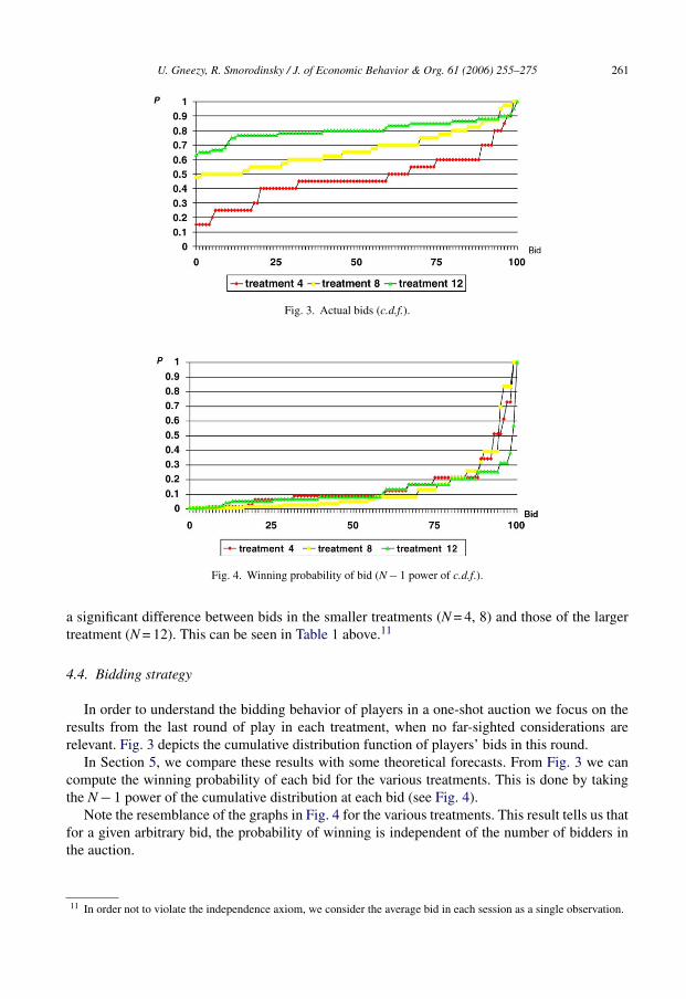
Fig. 3. Actual bids (c.d.f.).

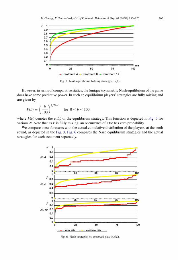
Fig. 4. Winning probability of bid (N − 1 power of c.d.f.).

a significant difference between bids in the smaller treatments (N = 4, 8) and those of the largertreatment (N = 12). This can be seen in Table 1 above.11

4.4. Bidding strategy

In order to understand the bidding behavior of players in a one-shot auction we focus on theresults from the last round of play in each treatment, when no far-sighted considerations arerelevant. Fig. 3 depicts the cumulative distribution function of players’ bids in this round.

In Section 5, we compare these results with some theoretical forecasts. From Fig. 3 we cancompute the winning probability of each bid for the various treatments. This is done by takingthe N − 1 power of the cumulative distribution at each bid (see Fig. 4).

Note the resemblance of the graphs in Fig. 4 for the various treatments. This result tells us thatfor a given arbitrary bid, the probability of winning is independent of the number of bidders inthe auction.

11 In order not to violate the independence axiom, we consider the average bid in each session as a single observation.


4.5. Winning bid

The winning bid was, for most rounds, quite close to the value of the prize. In fact, in 129 ofthe 150 rounds of play, the winning bid was 90 or more. Moreover, in 33 out of 150 rounds, thewinning bid was equal to 100, and in 8 rounds out of 150, the winning bid was strictly greaterthan 100. It is of interest to note that the average winning bid depicted in Fig. 4, is quite similarfor all 3 treatments. In fact the average winning bid, over all 10 rounds, was 91.2, 87.2, 95.3, forN = 4, 8, 12, respectively.

4.6. Number of participants

The number of players who submit a non-zero bid (active participants) at the first round of eachtreatment is monotonic increasing with N. For N = 4 there are 3.5 active participants on average,whereas for N = 12 there are more then 7. However, this monotonicity vanishes in later rounds ofplay. At the last round, for example, the average number of active participants is non-monotonicand is between 3.3 and 4.5 for all treatments.

4.7. Profiting players

Only 4 out of a total of 120 players left the experiment with a profit. Even then, profit wasnegligible (1, 5, 6.8 and 19 points after 10 rounds). Another 14 players made zero profit and 102players incurred actual losses.

5. Theoretical forecasts

In this section, we compare the results of our experiment to two forecasts based on two differenttheories. First, we consider the standard fully rational approach and compare the results to the Nashequilibrium forecasts. Second, we consider the Logit equilibrium model, studied by Andersonet al. (1998), as a representative of the boundedly rational approach. As we demonstrate in thesequel both theories fail to describe our results completely, nevertheless both theories conveysome intuition regarding the comparative statics we observe in the experiments.

In this section, we restrict attention to theories regarding behavior in the stage game. Con-sequently, the results of the experiment we focus on are those of the last (tenth) round in eachexperiment when no long run strategic considerations apply.

5.1. Nash equilibrium

Obviously, in order to study the Nash equilibria of a game, one must know the utility functionsof players. In the absence of these we shall consider two possibilities, first, that all players arerisk neutral, and second, that players are risk loving and have a logarithmic utility function.

5.1.1. Risk neutralityThe Nash equilibrium of the all-pay auction has been studied by Baye et al. (1996). We recall

some of their results. The game in study has multiple equilibria. One property that is common toall of these equilibria is that the expected seller’s revenue is equal to the (common) value of theprize. This stands in complete contrast to the results of the experiment (see Fig. 1).


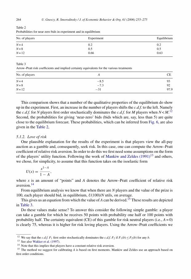
Fig. 5. Nash equilibrium bidding strategy (c.d.f.).

However, in terms of comparative statics, the (unique) symmetric Nash equilibrium of the gamedoes have some predictive power. In such an equilibrium players’ strategies are fully mixing andare given by

F (b) =(

b

100

)1/N−1

for 0 ≤ b ≤ 100,

where F(b) denotes the c.d.f. of the equilibrium strategy. This function is depicted in Fig. 5 forvarious N. Note that as F is fully mixing, an occurrence of a tie has zero probability.

We compare these forecasts with the actual cumulative distribution of the players, at the tenthround, as depicted in the Fig. 3. Fig. 6 compares the Nash equilibrium strategies and the actualstrategies for each treatment separately.

Fig. 6. Nash strategies vs. observed play (c.d.f.).


Table 2Probabilities for near zero bids in experiment and in equilibrium

No. of players Experiment Equilibrium

N = 4 0.2 0.2N = 8 0.5 0.5N = 12 0.66 0.63

Table 3Arrow–Pratt risk coefficients and implied certainty equivalents for the various treatments

No. of players A CE

N = 4 −8.5 93N = 8 −7.3 92N = 12 −31 97.9

This comparison shows that a number of the qualitative properties of the equilibrium do showup in the experiment. First, an increase in the number of players shifts the c.d.f. to the left. Namelythe c.d.f. for N players first order stochastically dominates the c.d.f. for M players when N < M.12

Second, the probabilities for giving ‘near-zero’ bids (bids which are, say, less than 5) are quiteclose to the equilibrium forecast. These probabilities, which can be inferred from Fig. 6, are alsogiven in the Table 2,

5.1.2. Love of riskOne plausible explanation for the results of the experiment is that players view the all-pay

auction as a gamble and, consequently, seek risk. In this case, one can compute the Arrow–Prattcoefficient of relative risk aversion. In order to do this we first need some assumptions on the formof the players’ utility function. Following the work of Mankiw and Zeldes (1991)13 and others,we chose, for simplicity, to assume that this function takes on the isoelastic form

U(x) = x1−A

1 − A,

where x is an amount of “points” and A denotes the Arrow–Pratt coefficient of relative riskaversion.14

From equilibrium analysis we know that when there are N players and the value of the prize is100, each player should bid, in equilibrium, U(100)/N utils, on average.

This gives us an equation from which the value of A can be derived.15 These results are depictedin Table 3.

Do these values make sense? To answer this consider the following simple gamble: a playercan take a gamble for which he receives 50 points with probability one half or 100 points withprobability half. The certainty equivalent (CE) of this gamble for risk neutral players (i.e., A = 0)is clearly 75, whereas it is higher for risk loving players. Using the Arrow–Pratt coefficients we

12 We say that the c.d.f. F1 first order stochastically dominates the c.d.f. F2 if F1(b) ≤ F2(b) for any b.13 See also Wakker et al. (1997).14 Note that this implies that players have a constant relative risk aversion.15 The method we suggest for calibrating A is based on first moments. Mankiw and Zeldes use an approach based on

first order conditions.


compute the values of CE (see Table 3). Obviously, these values are highly implausible, andconsequently we do not find the fully rational explanation of risk loving players as reasonable.

5.2. Logit equilibrium

A descriptive model of behavior intended to explain the over-bidding phenomenon in theall-pay auctions was recently given by Anderson et al. (1998). In their paper, following earlierliterature by McKelvey and Palfrey (1996) and Lopez (1995), the solution concept of the Logitequilibrium is used.

The Nash equilibrium solution concept is based on two assumptions. First, players are rational,that is, they take a best reply given their beliefs on the environment they live in (within ourframework, their belief on opponents’ behavior), and second, the beliefs comply with the truth. TheLogit equilibrium, on the other hand, only maintains the second assumption, namely compatibilityof beliefs and truth. This solution concept assumes players are boundedly rational. Bid decisionsare assumed to be determined by expected payoffs via a Logit probabilistic choice rule. Decisionswith higher expected payoffs are more likely to be chosen, but are not chosen with certainty (asin a Nash equilibrium).

We can now compare our laboratory results with the predictions of Anderson et al. (1998) forthe case of symmetric equilibrium strategies with a common value. In this scenario, Anderson etal. provide a closed form solution for the logit equilibrium as follows. Let F(b) denote a player’scumulative distribution function for his Logit equilibrium strategy, then

F (b)N−1 = a

VΓ (−1)

(1 − exp(−b/a)

1 − exp(−B/a)Γ

(V

a,

1

N − 1

),

1

N − 1

),

where V denotes the common value, B denotes the maximal bid allowed, Γ and Γ (−1) denote theincomplete gamma function and its inverse, respectively, (i.e., Γ (x, y) = fx

0 ty−1 exp(−t)dt), and0 < a < 1 is an ‘error’ parameter.16

5.2.1. Over-biddingAs is clearly seen in our results players overbid. This phenomenon is, qualitatively, projected

by the Logit equilibrium (see Proposition 6 in Anderson et al., who refer to this as ‘net rent’).The data from our experiment allows for a quantitative analysis. In our experiment, we witnessthat total revenues range from twice to five times the value of the prize. Thus, the net rent to theauctioneer ranges between 100 (at the last round with four players) and 400 (in first round with12 players). Computing the seller’s revenues, according to the Logit equilibrium forecast, as afunction of the noise factor, a, yields the following diagram:

We now compare actual overbidding (as presented in Fig. 1) with the Logit prediction (Fig. 7).In the first period of the experiment, the overbidding as well as the difference between treatmentsis consistent with the Logit equilibrium with a relatively large noise factor (a > 0.3). In the earlierrounds the over-bidding is also monotone with the numbers of players, as predicted by the Logitequilibrium.

In the later round, we notice two phenomenons. First, the seller’s revenue decreases, which canbe explained by a decrease of the noise factor a. The decrease in a is a plausible and appealinglearning model for Logit players.

16 Note that as the value of the noise factor, a, converges to zero, the Logit equilibrium converges to the Nash equilibriumand players put mass 1 on their best reply. However as a converges to 1, players reply randomly.


Fig. 7. Overbid in Logit equilibrium.

Fig. 8. Non-participation probability (probability of bids less or equal 5).

The second phenomenon undermines the Logit equilibrium model for the later stages of thegame. In later rounds overbidding ceases to be monotone in the number of participants (seller’srevenue is marginally higher for the N = 8 than for the N = 12 in the last round).17 This can beintuitively explained in a model where some players actually best reply as they learn, while otherskeep choosing their replies according to the Logit function (we elaborate in the next section).

To summarize, the Logit equilibrium forecast has proven a suitable model to explain ourresults in the early round. However, in later rounds, after players become experienced, the Logitequilibrium model fails to project the results of our experiment.

6. A Descriptive model of behavior

One model that can explain subjects’ bidding patterns in our experiment is a two-stage decisionproblem. Assume players in the auction decide on their bidding as follows, first, they decidewhether to participate or not, and second, given a decision to participate they decide on the bid.To test such an hypothesis we look at the following two figures. Fig. 8 demonstrates the probability

17 In fact, Anderson et al. recommend, in their conclusion, to test their theory in laboratory experiments by studyingwhether over-dissipation increases with the number of players.


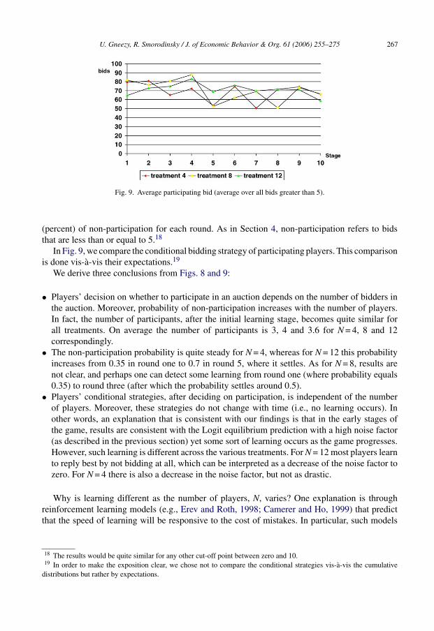
Fig. 9. Average participating bid (average over all bids greater than 5).

(percent) of non-participation for each round. As in Section 4, non-participation refers to bidsthat are less than or equal to 5.18

In Fig. 9, we compare the conditional bidding strategy of participating players. This comparisonis done vis-a-vis their expectations.19

We derive three conclusions from Figs. 8 and 9:

• Players’ decision on whether to participate in an auction depends on the number of bidders inthe auction. Moreover, probability of non-participation increases with the number of players.In fact, the number of participants, after the initial learning stage, becomes quite similar forall treatments. On average the number of participants is 3, 4 and 3.6 for N = 4, 8 and 12correspondingly.

• The non-participation probability is quite steady for N = 4, whereas for N = 12 this probabilityincreases from 0.35 in round one to 0.7 in round 5, where it settles. As for N = 8, results arenot clear, and perhaps one can detect some learning from round one (where probability equals0.35) to round three (after which the probability settles around 0.5).

• Players’ conditional strategies, after deciding on participation, is independent of the numberof players. Moreover, these strategies do not change with time (i.e., no learning occurs). Inother words, an explanation that is consistent with our findings is that in the early stages ofthe game, results are consistent with the Logit equilibrium prediction with a high noise factor(as described in the previous section) yet some sort of learning occurs as the game progresses.However, such learning is different across the various treatments. For N = 12 most players learnto reply best by not bidding at all, which can be interpreted as a decrease of the noise factor tozero. For N = 4 there is also a decrease in the noise factor, but not as drastic.

Why is learning different as the number of players, N, varies? One explanation is throughreinforcement learning models (e.g., Erev and Roth, 1998; Camerer and Ho, 1999) that predictthat the speed of learning will be responsive to the cost of mistakes. In particular, such models

18 The results would be quite similar for any other cut-off point between zero and 10.19 In order to make the exposition clear, we chose not to compare the conditional strategies vis-a-vis the cumulative

distributions but rather by expectations.


predict that the higher the costs, the faster the learning, which is exactly the case in our experimentas N increases from 4 to 12.

Anderson et al. (2002) have recently proposed a variation of the Logit model that is sensitiveto the asymmetric costs associated with deviations from the Nash equilibrium. Although theirmodel studies cost asymmetry within games, we believe that a similar argument can be made forcost asymmetry between games.

In fact, such a two-stage explanation can account for both phenomena observed. On the onehand, over-dissipation is explained by the Logit reaction functions. On the other hand, as thenumber of participants is quite similar for the various treatments (after an initial learning stage),the amount of over-dissipation becomes constant.

7. Conclusion

The all-pay auction has been widely studied because it is often used as an allocation mechanismin competitions for a prize where players’ effort involves the expenditure of resources. Examplesof such competitions are lobbying, research and development (R&D) competitions, monopolylicenses, franchises and others (e.g., Hillman and Samet, 1987 and Hillman, 1988).

In laboratory experiments of complete information all-pay auctions, players tend to over-bid. Infact, even after 10 rounds of play, the seller’s revenue amounts to between 2 and 3 times the valueof the prize. Furthermore, the seller’s revenue is almost independent of the number of players.

The observations reported here lack a complete theoretic foundation. The fully rationalapproach does not explain the over-bidding phenomenon or, alternatively, assumes quite implau-sible risk loving coefficients. The Logit equilibrium model, which assumes that players areboundedly rational, is suitable for explaining behavior in earlier rounds (assuming large noisefactors) but does not account for the independence of the seller’s revenue with respect to thenumber of players in later rounds.

One potential ad hoc explanation of the results is that players make their decisions in two stages,first, they decide whether to participate in the auction depending on the number of participantsand on past experience (i.e., on learning), and second, conditional on participating, players choosea bid independently of the number of participants and past experience (i.e., no learning).

Acknowledgements

We thank Mike Baye, Dan Levine, Lana Volokh and Stanislav (Sta) Rozenfeld and anonymousreferees for their comments. Financial support of the Technion VP of Research fund and by theJoint Research Foundation of the University of Haifa and the Technion is gratefully acknowledged.

Appendix A. Introduction form

You are about to participate in an experiment in decision-making. At the beginning, we willexplain to you the procedure of the experiment and then you will be asked to answer a questionnairechecking your understanding of the instructions. In the experiment, which is scheduled to take30 min, you will be asked to make some decisions. During the experiment, you will be earning“points”. These points will be converted to NIS at the end of the experiment, at the rate of 20points = 1 NIS. In other words 1000 points = 50 NIS. The exact amount you will earn depends onyour decisions, as well as the decisions made by other participants. The money you earn will bepaid to you at the end of the experiment, privately and in cash.


After reading these instructions, you will be asked to choose an envelope out of a box. Inthis envelope, you will find a note with your “registration number” on it. We ask you to memo-rize this number and put the note back into the envelope. Please be confidential regarding yourregistration number. You will need to write your number on the forms distributed during theexperiment, and also to present the number to us so we can pay you. One of the envelopes con-tains a note without a number. The holder of this note will be our “assistant” for the experiment.The assistant will not be participating in the experiment and will the average gain of al otherparticipants.

Note: After the distribution you are asked to remain silent. In case of discussion betweenparticipants, we shall have to abort the experiment.

Any questions?

Appendix B. Instructions form

Each participant has a credit of 1000 points in the beginning. The experiment is composedof 10 rounds. At each round, we shall “sell” 100 points in an auction. At the beginning of eachround, we shall ask each participant to write down his registration number as well as an amountof points on one of the notes you received. This amount is called a “bid” and will be deductedautomatically from your credit.

The assistant will collect the notes of all participants, and will read aloud the registration numberand bid of each participant. We will write these bids on the blackboard, and indicate which wasthe highest bid. The participant whose bid was the highest will “win” 100 points, and so he willadd them to his credit. In case of tie, we shall split the 100 points equally between all the highestplayers. Note that even if you do not win, your bid is nevertheless deducted from your credit.

At the end of round 1, we will continue to round 2, when your credit at round 2 depends onthe consequences of round one. Similarly for the following rounds.

Note: Please complete at the end of each round the form entitled “credit form”; your bid, theamount you win and your remaining credit. We also ask that your bid will never exceed yourcredit.

Appendix C. The quiz

Following are 6 multiple-choice questions designed to check your understanding of the instruc-tions. Please check only one answer for each question. Only students who will reply correctly toall questions are entitled to participate in the experiment.

1. Assume that in the first round your bid is 70 and you win:(a) You gain 30 in the first round(b) You gain 70 in the first round(c) You gain 130 in the first round(d) You loose 30 in the first round

2. Assume that in the first round your bid is 20 and you do not win:(a) You loose 20 in the first round(b) You gain 80 in the first round(c) You loose 120 in the first round(d) You loose 100 in the first round


3. Assume that in the first round your bid is 0 and you do not win:(a) You loose 100 in the first round(b) You gain 100 in the first round(c) You neither gain nor loose(d) Bidding 0 is not allowed

4. Assume that in the first round your bid is 90 and you do not win:(a) Your credit at the end of round 1 is 1090(b) Your credit at the end of round 1 is 1010(c) Your credit at the end of round 1 is 990(d) Your credit at the end of round 1 is 910

5. Assume that in the first round your bid is 90 and you do win:(a) Your credit at the end of round 1 is 1090(b) Your credit at the end of round 1 is 1010(c) Your credit at the end of round 1 is 990(d) Your credit at the end of round 1 is 910

6. Assume that in the first round your bid is 0 and you do not win:(a) Your credit at the end of round 1 is 1100(b) Your credit at the end of round 1 is 1000(c) Your credit at the end of round 1 is 900(d) None of the above

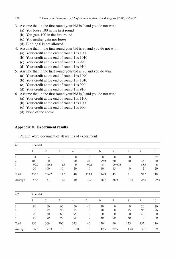
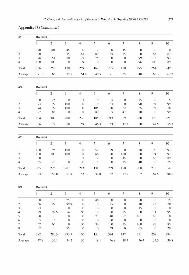
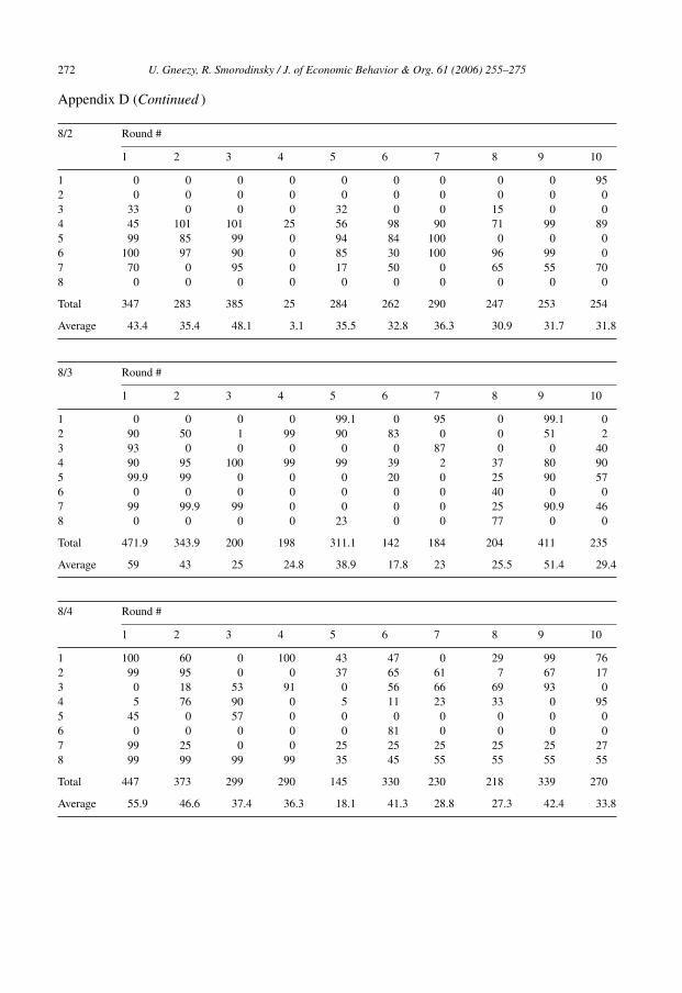
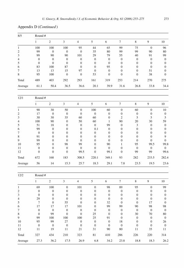
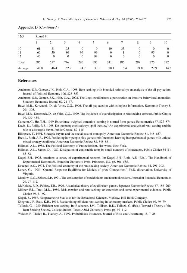
Appendix D. Experiment results

Plug in Word document of all results of experiment.

4/1 Round #

1 2 3 4 5 6 7 8 9 10

1 4 4 0 0 0 0 0 0 0 322 100 0 0 20 22 99.9 30 30 35 603 99.7 100.2 1.5 0 99.1 5 99.995 1 55.5 64 30 100 10 20 0 10 15 0 2 20

Total 233.7 204.2 11.5 40 121.1 114.9 145 31 92.5 118

Average 58.4 51.1 2.9 10 30.3 28.7 36.2 7.8 23.1 29.5

4/2 Round #

1 2 3 4 5 6 7 8 9 10

1 80 60 60 50 40 30 0 0 20 202 0 99 90 95 0 90 0 95 95 963 20 60 60 95 0 0 0 0 40 04 50 90 90 95 0 50 90 80 0 0

Total 150 309 300 335 40 170 90 175 155 116

Average 37.5 77.3 75 83.8 10 42.5 22.5 43.8 38.8 29


Appendix D (Continued )

4/3 Round #

1 2 3 4 5 6 7 8 9 10

1 90 101 45 0 7 0 15 0 0 02 0 0 15 65 80 85 85 0 85 673 96 51 70 95 75 100 0 99 76 934 100 100 0 99 0 100 0 96 100 89

Total 286 252 130 259 162 285 100 195 261 249

Average 71.5 63 32.5 64.8 40.5 71.3 25 48.8 65.3 62.3

4/4 Round #

1 2 3 4 5 6 7 8 9 10

1 0 25 0 35 0 5 0 75 0 52 93 99 100 0 0 33 0 90 97 993 74 99 100 100 105 90 22 85 93 184 97 85 0 101 80 85 47 70 0 99

Total 264 308 200 236 185 213 69 320 190 221

Average 66 77 50 59 46.3 53.3 17.3 80 47.5 55.3

4/5 Round #

1 2 3 4 5 6 7 8 9 10

1 100 95 100 101 50 99 0 28 90 932 100 100 100 105 66 90 100 60 94 973 80 0 7 7 7 80 15 80 86 894 55 28 0 0 8 0 35 40 0 75

Total 335 223 207 213 131 269 150 208 270 354

Average 83.8 55.8 51.8 53.3 32.8 67.3 37.5 52 67.5 88.5

8/1 Round #

1 2 3 4 5 6 7 8 9 10

1 0 15 25 0 46 0 0 0 0 152 36 97 99.9 0 0 95 0 10 22 703 93 0 0 0 0 0 0 15 0 04 99 99.5 54 60 0 80 55 0 71 955 0 0 0 0 77 40 57 101 80 06 5 3 0 0 0 0 0 0 0 07 52 66 0 100 30 100 35 100 95 858 97 0 95 0 0 59 0 65 0 29

Total 382 280.5 273.9 160 153 374 147 291 268 294

Average 47.8 35.1 34.2 20 19.1 46.8 18.4 36.4 33.5 36.8



8/2 Round #

1 2 3 4 5 6 7 8 9 10

1 0 0 0 0 0 0 0 0 0 952 0 0 0 0 0 0 0 0 0 03 33 0 0 0 32 0 0 15 0 04 45 101 101 25 56 98 90 71 99 895 99 85 99 0 94 84 100 0 0 06 100 97 90 0 85 30 100 96 99 07 70 0 95 0 17 50 0 65 55 708 0 0 0 0 0 0 0 0 0 0

Total 347 283 385 25 284 262 290 247 253 254

Average 43.4 35.4 48.1 3.1 35.5 32.8 36.3 30.9 31.7 31.8

8/3 Round #

1 2 3 4 5 6 7 8 9 10

1 0 0 0 0 99.1 0 95 0 99.1 02 90 50 1 99 90 83 0 0 51 23 93 0 0 0 0 0 87 0 0 404 90 95 100 99 99 39 2 37 80 905 99.9 99 0 0 0 20 0 25 90 576 0 0 0 0 0 0 0 40 0 07 99 99.9 99 0 0 0 0 25 90.9 468 0 0 0 0 23 0 0 77 0 0

Total 471.9 343.9 200 198 311.1 142 184 204 411 235

Average 59 43 25 24.8 38.9 17.8 23 25.5 51.4 29.4

8/4 Round #

1 2 3 4 5 6 7 8 9 10

1 100 60 0 100 43 47 0 29 99 762 99 95 0 0 37 65 61 7 67 173 0 18 53 91 0 56 66 69 93 04 5 76 90 0 5 11 23 33 0 955 45 0 57 0 0 0 0 0 0 06 0 0 0 0 0 81 0 0 0 07 99 25 0 0 25 25 25 25 25 278 99 99 99 99 35 45 55 55 55 55

Total 447 373 299 290 145 330 230 218 339 270

Average 55.9 46.6 37.4 36.3 18.1 41.3 28.8 27.3 42.4 33.8



8/5 Round #

1 2 3 4 5 6 7 8 9 10

1 100 100 100 95 44 65 99 75 0 962 99 0 0 0 35 80 99 99 90 803 99 90 90 101 29 79 55 40 91 994 0 0 0 0 0 0 0 0 0 05 0 0 0 0 0 0 0 0 0 06 83 100 87 0 0 95 0 0 0 07 13 13 15 97 0 0 0 0 51 08 95 100 0 0 53 0 0 0 38 0

Total 489 403 292 293 161 319 253 214 270 275

Average 61.1 50.4 36.5 36.6 20.1 39.9 31.6 26.8 33.8 34.4

12/1 Round #

1 2 3 4 5 6 7 8 9 10

1 90 30 50 0 100 60 0 60 0 102 17 0 0 0 0 0 0 0 0 03 30 30 35 60 60 0 2 5 5 54 100 90 0 50 60 1 90 20 30 595 51 18 0 0 0 99 0 3 0 06 99 0 0 0 0.1 0 0 0 0 07 0 0 0 0 0 0 0 0 0 08 91 0 0 0 0 0 0 0 0 99 99 0 0 0 0 0 0 0 0 010 95 0 98 99 0 90 1 95 99.5 99.811 0 0 0 0 0 0 0 0 0 012 0 0 0 99.5 0 99.1 0 99 99 99.6

Total 672 168 183 308.5 220.1 349.1 93 282 233.5 282.4

Average 56 14 15.3 25.7 18.3 29.1 7.8 23.5 19.5 23.6

12/2 Round #

1 2 3 4 5 6 7 8 9 10

1 69 100 0 101 0 98 89 95 0 992 0 0 0 0 0 0 0 0 0 03 0 0 0 0 0 0 0 0 0 04 29 0 0 0 0 0 0 0 0 05 7 0 55 0 0 32 0 0 17 06 17 17 17 101 0 99 99 90 98 987 0 0 0 0 0 0 0 0 0 08 0 99 0 0 25 0 0 30 70 809 99 100 100 100 25 91 0 0 0 010 95 99 27 0 0 0 18 0 0 2611 0 0 0 0 0 0 0 0 0 012 11 19 11 21 31 90 80 11 35 11

Total 327 434 210 323 81 410 286 226 220 314

Average 27.3 36.2 17.5 26.9 6.8 34.2 23.8 18.8 18.3 26.2



12/3 Round #

1 2 3 4 5 6 7 8 9 10

1 90 90 0 0 0 0 0 0 0 02 50 0 78 90 0 0 0 0 0 03 0 0 0 100 100 0 10 0 0 04 99 0 0 99 10 0 0 101 0 15 0 0 0 0 0 0 0 0 0 06 0 80 90 90 91 90 90 0 0 07 60 60 0 100 100 100 100 100 100 1008 0 0 0 0 0 0 0 0 0 09 0 55 80 0 0 0 0 0 105 1010 0 100 0 99 0 0 0 0 0 011 0 99 0 0 0 0 0 0 0 012 92 0 0 0 0 0 0 0 0 0

Total 391 484 248 578 301 190 200 201 205 111

Average 32.6 40.3 20.7 48.2 25.1 15.8 16.7 16.8 17.1 9.3

12/4 Round #

1 2 3 4 5 6 7 8 9 10

1 0 0 0 0 0 0 0 0 0 02 17 91 101 36 0 0 0 5 10 113 23 0 0 0 0 0 101 87 0 04 99 79 0 0 0 0 0 0 0 05 90 100 91 71 15 15 0 85 0 886 77 93 0 0 0 27 0 0 95 677 16 26 36 46 86 96 100 53 100 408 5 0 0 0 0 99 0 0 0 09 77 77 77 77 77 0 89 0 0 9510 0 0 0 0 0 0 0 0 0 011 87 0 100 95 60 95 0 65 0 012 0 0 0 0 0 0 0 0 0 0

Total 491 466 405 325 238 332 290 295 205 301

Average 41 38.9 33.8 27.1 19.8 27.7 24.2 24.6 17.1 25.1

12/5 Round #

1 2 3 4 5 6 7 8 9 10

1 0 92 95 0 0 100 0 0 0 02 90 0 99 0 0 0 1 91 0 993 86 93 95 99 99 31 35 47 0 134 75 60 97 0 100 100 40 60 80 605 10 90 90 0 0 0 70 0 90 06 53 91 0 0 0 0 0 0 0 07 40 0 0 98 0 0 0 0 0 08 0 0 0 0 0 0 0 99 0 09 70 0 95 0 0 0 5 0 10 0



12/5 Round #

1 2 3 4 5 6 7 8 9 10

10 61 81 95 0 0 10 33 0 0 011 60 50 80 99 99 0 1 0 95 012 40 0 0 0 99 0 0 0 0 0

Total 585 557 746 296 397 241 185 297 275 172

Average 48.8 46.4 62.2 24.7 33.1 20.1 15.4 24.8 22.9 14.3

References

Anderson, S.P., Goeree, J.K., Holt, C.A., 1998. Rent seeking with bounded rationality: an analysis of the all-pay uction.Journal of Political Economy 106, 828–853.

Anderson, S.P., Goeree, J.K., Holt, C.A., 2002. The Logit equilibrium: a perspective on intuitive behavioral anomalies.Southern Economic Journal 69, 21–47.

Baye, M.R., Kovenock, D., de Vries, C.G., 1996. The all-pay auction with complete information. Economic Theory 8,291–305.

Baye, M.R., Kovenock, D., de Vries, C.G., 1999. The incidence of over dissipation in rent seeking contests. Public Choice99, 439–454.

Camerer, C., Ho, T.H., 1999. Experience-weighted attraction learning in normal form games. Econometrica 67, 827–874.Davis, D., Reilly, R.J., 1998. Do too many cooks always spoil the stew? An experimental analysis of rent-seeking and the

role of a strategic buyer. Public Choice, 89–115.Ellingsen, T., 1991. Strategic buyers and the social cost of monopoly. American Economic Review 81, 648–657.Erev, I., Roth, A.E., 1998. Predicting how people play games: reinforcement learning in experimental games with unique,

mixed strategy equilibria. American Economic Review 88, 848–881.Hillman, A.L., 1988. The Political Economy of Protectionism. Har-wood, New York.Hillman, A.L., Samet, D., 1987. Dissipation of contestable rents by small numbers of contenders. Public Choice 54 (1),

63–82.Kagel, J.H., 1995. Auctions: a survey of experimental research. In: Kagel, J.H., Roth, A.E. (Eds.), The Handbook of

Experimental Economics. Princeton University Press, Princeton, N.J, pp. 501–585.Krueger, A.O., 1974. The Political economy of the rent seeking society. American Economic Review 64, 291–303.Lopez, G., 1995. “Quantal Response Equilibria for Models of price Competition.” Ph.D. dissertation, University of

Virginia.Mankiw, N.G., Zeldes, S.P., 1991. The consumption of stockholders and nonstockholders. Journal of Financial Economics

29, 97–112.McKelvey, R.D., Palfrey, T.R., 1996. A statistical theory of equilibrium games. Japanese Economic Review 47, 186–209.Millner, E.L., Pratt, M.D., 1989. Risk aversion and rent-seeking: an extension and some experimental evidence. Public

Choice 69, 81–92.Siegel, S., 1956. Nonparametric Statistics for the Behavioral Sciences. McGraw-Hill Book Company.Shogren, J.F., Baik, K.H., 1991. Reexamining efficient rent-seeking in laboratory markets. Public Choice 69, 69–79.Tullock, G., 1980. Efficient rent seeking. In: Buchanan, J.M., Tollison, R.D., Tullock, G. (Eds.), Toward a Theory of the

Rent Seeking Society. College Station: Texas A&M University Press, pp. 97–112.Wakker, P., Thaler, R., Tversky, A., 1997. Probabilistic insurance. Journal of Risk and Uncertainty 15, 7–28.

Documents

All-pay auctions—an experimental studyrady.ucsd.edu/faculty/directory/gneezy/pub/docs/all-pay-auctions.pdf · In an all-pay auction, the winner is determined according to the highest