Alignment and sub-pixel interpolation of images usingFourier methods

C.A. GlasbeyBiomathematics and Statistics Scotland

King’s Buildings, Edinburgh, EH9 3JZ, Scotland

andG.W.A.M. van der Heijden

BiometrisP.O. Box 16, 6700 AA Wageningen, The Netherlands

Abstract

A method is proposed for both estimating and correcting a translational mis-alignmentbetween digital images, taking account of aliasing of high-frequency information. A para-metric model is proposed for the power- and cross-spectra of the multivariate stochasticprocess that is assumed to have generated a continuous-space version of the images. Pa-rameters, including those that specify mis-alignment, are estimated by numerical max-imum likelihood. The effectiveness of the interpolant is confirmed by simulation andillustrated using multi-band Landsat images.

Key words: Aliasing, Coherency, Complex Gaussian distribution, Cross-spectrum, Land-sat image, Phase spectrum, Power spectrum, Sub-pixel.

1 Introduction

A digital image consists of a set of pixels, which are typically sampled points on a rectangularspatial lattice. The sampling involves a spatial convolution or smoothing of a process in contin-uous space, plus the addition of noise. In image analysis we often need values of the process atnon-lattice points, mainly for image enlargement (zooming). These values are usually obtainedby interpolation, which implicitly assumes that it is sufficient to recover the smoothed versionof the process and that noise is negligible. Standard interpolation methods include the bilinear,bicubic and b-spline interpolators. The sinc interpolator is optimal if sampling is in accordwith the Nyquist criterion, i.e. the sampling frequency is two times the highest frequency in thesmoothed process. However, if the image contains aliasing, the sinc interpolator is not optimal.

1

A general theory for optimal linear interpolation is provided by kriging Parrott et al. (1993).For a recent review of image interpolation, see Meijering (2002).

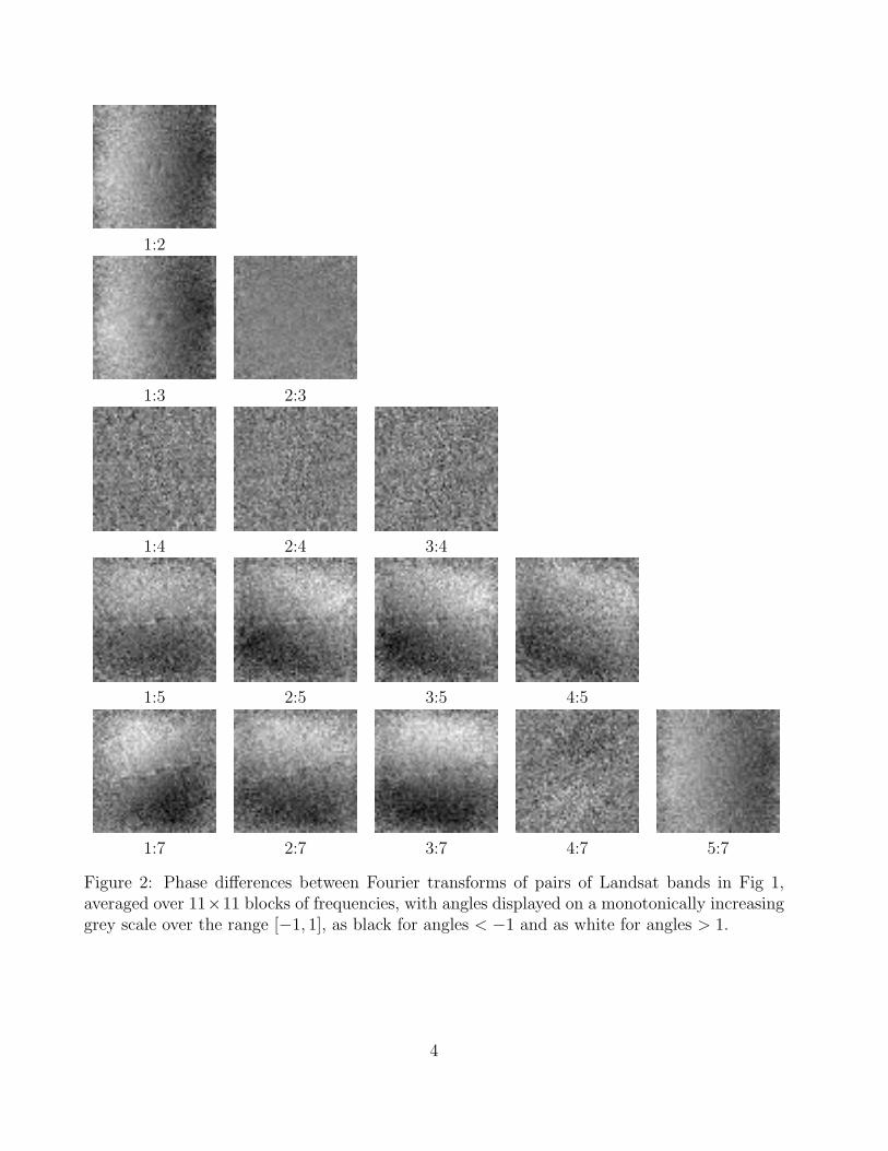
As well as for enlargement, another reason for interpolation is to align images which havesub-pixel translation shifts. For example, microscope images obtained using different imagingmodalities can be translationally shifted Glasbey and Mardia (2001), as can the different bandsin remotely sensed images (Berman et al., 1994). To illustrate the second case, consider bands1-5 and 7 of a Landsat TM image, shown in Fig 1 and previously analysed by Glasbey andHorgan (1995). Fig 2 shows phase differences between Fourier transforms of all pairs of Landsatbands, in which translations between bands manifest themselves as linear trends (see §2 forfurther details). We see evidence for bands 2 and 3 being translated horizontally relative toband 1, band 5 being translated vertically and band 7 being translated diagonally. We notethat these trends cover the full range of frequencies except for tapering to zero at the highestfrequencies. This means that noise is negligible in these bands, and the tapering effect is dueto aliasing. Band 7 also appears to be translated vertically relative to bands 2 and 3 andtranslated horizontally relative to band 5. In such cases, there is a need both to estimate thetranslation, and to correct for it by interpolation.

Estimation of a translation is most elegantly done in the Fourier domain. For example, usingFourier transforms the cross-correlation between images at all translations that are whole num-bers of pixels can be computed simultaneously. Berman et al. (1994) took account of aliasingby empirically modelling the effect on phase differences. Kaltenbacher and Hardie (1996) andLuengo Hendriks and van Vliet (2000) estimated sub-pixel translations by approximating oneimage by a first-order Taylor series expansion of a second image.

After estimating the translation, interpolation is possible to sub-pixel accuracy, by making useof cross-correlation between images. This is often referred to as super-resolution (Hunt, 1995).One special case is where the shifted images are sampled from a common process, for examplewhere movement of a camera provides sub-pixel shifted frames. Several methods have beenproposed (Borman and Stevenson, 1998; Luengo Hendriks and van Vliet, 2000), which can beused to increase the resolution of camera images. Another special case is digital colour imaging,where a colour mosaic filter is used to obtain red, green and blue bands, the misalignmentbetween bands is known, but there is still a need to correct for it by interpolation, and anopportunity to use the information from the other colour bands. The most common colourmosaic filter is the Bayer filter, where every second pixel in a chequerboard pattern is greenand the others alternate between red and blue pixels. A common approach to interpolate thesecolour images is demosaicking, developed by Freeman (1988). Bands are interpolated usinga standard interpolator, such as bilinear interpolation, and then a median filter is applied tothe difference image of e.g. red-green and blue-green. A mathematical framework is proposedby Trussel and Hartwig (2002), and Ramanath et al. (2002) describe this and several otherapproaches.

In this paper we propose an approach which simultaneously estimates the amount of aliasing,the misalignment between the images, and the coherency between them. The estimated pa-rameters are used to create a powerful interpolant and also to align the images. The methodis formulated in §2, and applied to the Landsat data in §3. Finally, in §4, the methodology isdiscussed.

2

band 1 band 2

band 3 band 4

band 5 band 7

Figure 1: Landsat Thematic Mapper (TM) images: bands 1-5 and 7, for a region between theriver Tay and the town of St Andrews on the east coast of Scotland, in May 1987. There are512 × 512 pixels, each 302m. ( c©National Remote Sensing Centre Ltd, Farnborough, Hamp-shire.)

3

1:2

1:3 2:3

1:4 2:4 3:4

1:5 2:5 3:5 4:5

1:7 2:7 3:7 4:7 5:7

Figure 2: Phase differences between Fourier transforms of pairs of Landsat bands in Fig 1,averaged over 11×11 blocks of frequencies, with angles displayed on a monotonically increasinggrey scale over the range [−1, 1], as black for angles < −1 and as white for angles > 1.

4

2 Method

Let Fj,xy denote the pixel value at spatial location (x, y) in the jth of J digital images, for integervalues of x = 0, . . . , (K − 1), y = 0, . . . , (L − 1). We assume that sampling noise is negligible,so that these are sampled values on the integer lattice of an unobserved smoothed process (f)in continuous space, with Fj,xy ≡ fj(x, y). We further assume that f(x, y) is a realisation ofJ stationary, cross-correlated, stochastic processes on a continuous 2D rectangular domain:0 ≤ x < K and 0 ≤ y < L.

The Fourier representation of fj is

fj(x, y) =∞∑

k=−∞

∞∑l=−∞

f ∗j,kl exp

[2πι

(xk

K+

yl

L

)], (1)

where ι denotes√−1 and f ∗

j,kl is the complex Fourier transform of fj at frequency ωkl ≡(ω1,kl, ω2,kl)

T = 2π( kK

, lL)T . As K,L → ∞, the Fourier coefficients (f ∗) converge in distribu-

tion to multivariate complex normal distributions, independently distributed at each frequencyexcept for 180◦ rotational symmetry (i.e. f ∗

j,−k,−l ≡ f ∗j,kl, where f ∗ denotes the complex con-

jugate). For an introduction to complex distributions see, for example, Andersen et al. (1995,ch. 2). At frequency ωkl, the J Fourier coefficients, f ∗

1,kl, . . . , f∗J,kl, which we abbreviate to f ∗

kl,have zero mean and J × J complex variance matrix, vkl. So, for example,

cov

([ R(f ∗i,kl)

I(f ∗i,kl)

],

[ R(f ∗j,kl)

I(f ∗j,kl)

])=

1

2

[ R(vij,kl) −I(vij,kl)I(vij,kl) R(vij,kl)

], (2)

where R(z) and I(z) denote the real and imaginary parts of complex variable, z. In particular,terms vjj,kl (for k, l = −∞, . . . ,∞), which are real, are the power spectrum of fj, and vij,kl

(i 6= j) is the cross-spectrum between fi and fj, which is complex, and can be represented as

vij,kl = |vij,kl| eι φij,kl , where φij,kl = arg(vij,kl) ≡ tan−1

( I(vij,kl)

R(vij,kl)

), (3)

where |z| and arg(z) denote, respectively, the modulus and argument (or phase) of complexvariable z. Terms |vij,kl|, for k, l = −∞, . . . ,∞, are the cross-amplitude spectrum, and termsφij,kl are the phase spectrum, between fi and fj. The coherency,

ρij,kl =|vij,kl|√

vii,kl vjj,kl

, (4)

lies in the interval [0, 1], and is a measure of correlation between fi and fj at frequency ωkl.(For further on all the above, in the 1-D case, see, for example, Bloomfield, 2000, ch. 4.)

Translations in the spatial domain are equivalent to phase differences in the Fourier domain.Therefore, if images are misaligned due to translations, the phase spectra will be linear functionsof ω. In particular, if image j is misaligned with respect to image 1 by µj ≡ (µ1,j, µ2,j)

T pixels(i.e. µ1,j pixels in the x-direction and µ2,j pixels in the y-direction), then the misalignmentbetween images i and j will be (µi − µj) pixels, and

φij,kl = ωTkl (µi − µj) mod 2π. (5)

5

The Fourier representation of the observed data, F , is

Fj,xy =

K2−1∑

k=−K2

L2−1∑

l=−L2

F ∗j,kl exp

[2πι

(xk

K+

yl

L

)](6)

where the inverse Fourier transform is

F ∗j,kl =

1

KL

K−1∑x=0

L−1∑y=0

Fj,xy exp

[−2πι

(xk

K+

yl

L

)]. (7)

Note that the k and l summations are over finite ranges, unlike in (1), and there are only afinite number of Fourier coefficients, F ∗, which are related to f ∗ by

F ∗j,kl =

∞∑p=−∞

∞∑q=−∞

f ∗j,k+Kp,l+Lq, k = −K

2, . . . ,

(K

2− 1

), l = −L

2, . . . ,

(L

2− 1

). (8)

All coefficients at frequencies beyond half the sampling frequency (i.e. |ω1| or |ω2| > π), arealiased with coefficients at lower frequencies. Since the Fourier coefficients F ∗ are linear combi-nations of asymptotically independently distributed complex random variables f ∗, they are alsoapproximately multivariate normally distributed, with zero mean, complex variance V , where

Vkl =∞∑

p=−∞

∞∑q=−∞

vk+Kp,l+Lq , (9)

and the log likelihood of F can be approximated by

L = −1

2

K2−1∑

k=−K2

L2−1∑

l=−L2

(log |Vkl| + (F ∗

kl)T V −1

kl F ∗kl

). (10)

The asymptotic approximation can be improved by tapering the borders of images using acosine bell before obtaining Fourier coefficients (Bloomfield, 2000, §6.2).

We model the power spectra (vjj) by

vjj,kl = g(ωkl, αj), (11)

and coherencies (ρij) byρij,kl = h(ωkl, βij), (12)

where g and h are functions, which will vary with application, with unknown sets of parametersα and β. In combination, (5), (11) and (12) specify variance matrices vkl and Vkl at all fre-quencies ωkl. We estimate parameters µ, α and β, by numerically maximising the asymptoticlog likelihood (L) given by (10). However, note that in specific situations some parameters willbe of known value. For example, if data are multiple copies of a single image, then coherenciesρ ≡ 1. For colour images produced using e.g. a Bayer colour mosaic filter, the misalignment(µ) between bands will be known.

6

Once parameters are estimated, we can infer the smoothed process in continuous space, f ,and thereby correct for translation and interpolate. We first obtain estimates for the de-aliased Fourier terms, conditional on the observed terms, for k = −K/2, . . . , K/2 − 1; l =−L/2, . . . , L/2 − 1:

f̂ ∗k+Kp,l+Lq = v̂k+Kp,l+Lq V̂ −1

kl F ∗kl p = −P, . . . , P, q = −Q, . . . , Q, (13)

where P and Q are chosen to be sufficiently large that v̂k+Kp,l+Lq is negligible for |p| > P or|q| > Q. This follows from Mardia et al. (1979, p. 63). Then we apply a phase adjustment,

f̂ ∗j,kl → f̂ ∗

j,kl × exp[−ι ωTkl µj] (14)

for all j, k, l, to reverse the translation. Finally, the inverse Fourier transform produces alignedimages at sub-pixel resolution, which can be further interpolated using the sinc function.

3 Application

3.1 Model identification

Before we can apply the methodology of §2 to the Landsat bands shown in Fig 1, we needto use F ∗ to identify appropriate models for the power spectra and coherencies. We consider,in turn, displays and plots to identify the power spectra (vjj,kl), confirm the model for phasespectra (φij,kl) and identify the model for coherencies (ρij,kl). To do this, we assume at theidentification stage that aliasing is not too severe, so

Vkl ≈ vkl, (15)

for |ωkl| not too near π.

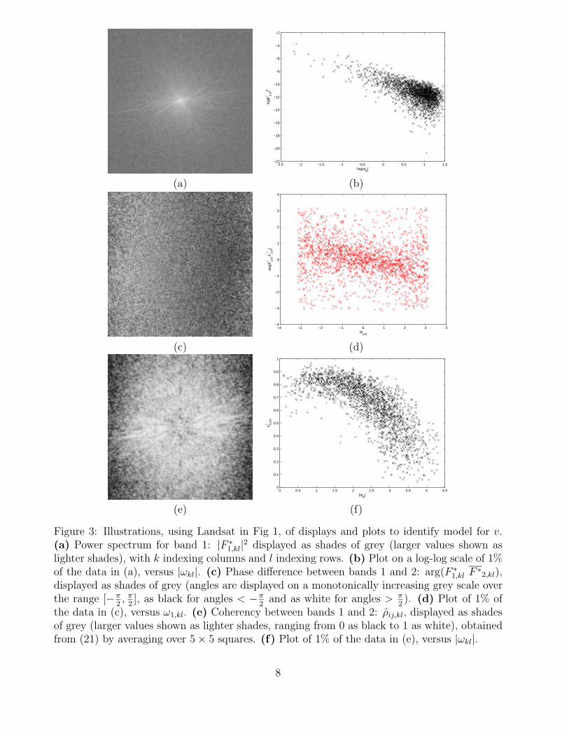
Fig 3(a) shows an image representation of |F ∗1,kl|2, obtained from Landsat band 1 after tapering

of the image boundaries using a cosine bell. Because

E|F ∗j,kl|2 = Vjj,kl ≈ vjj,kl, (16)

where E denotes expectation, this display helps us choose a model for the power spectrum. AsFig 3(a) and similar displays for the remaining bands (not shown), show approximate circularsymmetry, we assume that vkl is simply a function of |ωkl|. Fig 3(b) shows a log-log plot of|F ∗

1,kl|2 against |ωkl| for a random 1% of the values, the linearity of which is supportive of amodel of the form

vjj,kl = αj,1 |ωkl|αj,2 , (17)

where α are unknown parameters to be estimated. Others have advocated the 2D Maternfunction (Handcock and Wallis, 1994; Stein, 1999),

vjj,kl =θj,1

(θj,2 + |ωkl|2)θj,3+1, (18)

7

−2.5 −2 −1.5 −1 −0.5 0 0.5 1 1.5−22

−20

−18

−16

−14

−12

−10

−8

−6

−4

−2

log|

F* 1,

kl|2

log|ωkl

|

(a) (b)

−4 −3 −2 −1 0 1 2 3 4−4

−3

−2

−1

0

1

2

3

4

ω1,kl

arg(

F* 1,

kl F

−* 2,kl

)

(c) (d)

0 0.5 1 1.5 2 2.5 3 3.5 4 4.50

0.1

0.2

0.3

0.4

0.5

0.6

0.7

0.8

0.9

1

|ωkl

|

ρ^ 12,k

l

(e) (f)

Figure 3: Illustrations, using Landsat in Fig 1, of displays and plots to identify model for v.(a) Power spectrum for band 1: |F ∗

1,kl|2 displayed as shades of grey (larger values shown aslighter shades), with k indexing columns and l indexing rows. (b) Plot on a log-log scale of 1%of the data in (a), versus |ωkl|. (c) Phase difference between bands 1 and 2: arg(F ∗

1,kl F ∗2,kl),

displayed as shades of grey (angles are displayed on a monotonically increasing grey scale overthe range [−π

2, π

2], as black for angles < −π

2and as white for angles > π

2). (d) Plot of 1% of

the data in (c), versus ω1,kl. (e) Coherency between bands 1 and 2: ρ̂ij,kl, displayed as shadesof grey (larger values shown as lighter shades, ranging from 0 as black to 1 as white), obtainedfrom (21) by averaging over 5 × 5 squares. (f) Plot of 1% of the data in (e), versus |ωkl|.

8

but our experience in fitting (18) to image data is that θ̂j,2 ≈ 0 (Glasbey, 2001), which can leadto problems in its use.

Fig 3(c) shows an image representation of the phase differences between Landsat bands 1 and2, i.e. arg(F ∗

1,kl) − arg(F ∗2,kl) ≡ arg(F ∗

1,kl F ∗2,kl), which are estimates of φ12,kl because

E(F ∗i,kl F ∗

j,kl) = Vij,kl ≈ vij,kl ≡ |vij,kl| eι φij,kl . (19)

A linear trend from left to right can be discerned in Fig 3(c), except towards the edges ofthe display where the approximation breaks down because of aliasing with higher frequencies.Fig 3(d) shows phase differences plotted against ω1,kl for 1% of the values, and again a lineartrend can be seen. These displays, and similar ones for other comparisons of pairs of Landsatbands, support the linear model for the phase spectra, given in (5)

The coherencies (ρij) are symmetric in i and j, and ρjj ≡ 1, so we need only consider i < j. Ourstrategy is to model the coherencies only for i = (j − 1), and otherwise to model conditionalcoherencies (γij) between non-adjacent bands. For i ≤ (j − 2), let γij denote the coherencybetween bands i and j conditional on bands (i+1), (i+2), . . . , (j−1). From the set of coherenciesand conditional coherencies at frequency ωkl, Appendix 1 shows how we obtain matrix |vkl|,which gives terms in the cross-amplitude spectra. By constraining ρ ∈ [0, 1] and γ ∈ [−1, 1],we ensure that all |v| are positive definite.

From (19), (4) and (16),

|E(F ∗i,kl F ∗

j,kl)| ≈ |vij,kl| ≡ ρij,kl√

vii,kl vjj,kl ≈ ρij,kl

√E|F ∗

i,kl|2 E|F ∗j,kl|2. (20)

However, unlike for vjj,kl and φij,kl, we cannot obtain an estimate for ρij,kl using only F ∗i,kl and

F ∗j,kl, because |F ∗

i,kl F ∗j,kl| ≡ |F ∗

i,kl| |F ∗j,kl|. Therefore, we instead combine information over a

small range of frequencies, to obtain

ρ̂ij,kl =|∑pq F ∗

i,pq F ∗j,pq|√

(∑

pq |F ∗i,pq|2) (

∑pq |F ∗

j,pq|2), (21)

where the summations are over the set { (p, q) : (k−n) ≤ p ≤ (k +n), (l−n) ≤ q ≤ (l+n) },a (2n + 1)-square centred on (k, l) for a small value such as n = 2 or 3. Fig 3(e) shows animage representation of the estimated coherency between Landsat bands 1 and 2. As Fig 3(e)and similar displays for other pairs of bands (not shown), exhibit circular symmetry, we assumethat the coherency is simply a function of |ωkl|. Fig 3(f) shows a plot of estimated coherencyagainst |ωkl| for 1% of the values, which suggests a curvilinear relationship, that we can modelusing a second-order polynomial.

To ensure that coherencies lie in the interval [0, 1] we use a logistic link function. So, forcoherencies between adjacent bands:

ρ(j−1),j,kl =1

1 + exp[∑2

m=0 β(j−1),j,m|ωkl|m], (22)

where β(j−1),j are unknown parameters to be estimated. For simplicity and to limit the num-ber of parameters, we assume that the conditional coherencies (γ) are each constant over all

9

µ̂2 µ̂3 µ̂4 µ̂5 µ̂7

0.31 0.33 0.36 0.05 0.290.03 −0.02 −0.02 0.45 0.47

Table 1: Estimated misalignment between Landsat band 1 and other bands.

frequencies, so, to ensure that they lie in the interval [−1, 1], we specify

γij,kl =1 − eβij

1 + eβij, (23)

where βij are also unknown parameters to be estimated.

3.2 Results

We fit the model specified by (17), (22) and (23) to the 6 Landsat bands shown in Fig 1by numerically maximising L, after having initialised the 47 parameters as follows. The 10parameters (µ) in the relative shift of each band relative to band 1 were all initialised at0. The 12 parameters (α) in the power spectrum model were initialised by linear regression,ignoring aliasing. The coherency between adjacent bands required 15 parameters and theconditional coherencies a further 10 parameters (β). These were all initialised at 0, whichimplies a coherency between bands i and j of 0.5|i−j|.

We used a quasi-Newton constrained function minimisation routine with Sequential QuadraticProgramming, where an estimate of the Hessian of the Lagrangian function is updated at eachiteration using the Broyden-Fletcher-Goldfarb-Shanno (BFGS) formula (Matlab 12.1 Referencemanual, 2001). The calculation of the likelihood was written in a compiled C-routine, to speedup the estimation process. To simplify computation of L, we assumed f was band-limitedat the sampling frequency, i.e. f ∗

j,kl ≡ 0 for |ω1| or |ω2| > 2π, and therefore we have twofoldundersampling with respect to the Nyquist criterion. We omitted Fourier coefficients at thelowest frequencies (|ω| < 0.10π) from L, since some of these terms are very large and so candominate the estimation of α, whereas frequencies in the range 0.25π to 1.75π are more relevantfor interpolation. Also, to speed up the computations, we used only a random 10% of the Fouriercoefficients. These proved to be sufficient to obtain good estimates of all parameters. A singlelikelihood calculation using 20,000 frequencies took about 4 seconds on a Pentium 4-1500 MHzPC, and the algorithm converged after 100 iterations, and required 5200 evaluations of LFig 4 illustrates the model fit by showing plots matching those in Fig 3. The estimated shiftsbetween the bands are given in Table 1. These are consistent with what we saw in Fig 2, withbands 2 and 3 misaligned horizontally by 1/3rd of a pixel relative to band 1, band 5 misalignedvertically by almost half a pixel and band 7 misaligned diagonally. In addition, we see thatband 4 is misaligned horizontally by 1/3rd of a pixel.

To illustrate the results of interpolation, Fig 5 shows details of two small regions in the band7 image. For comparison, we also show the results of bicubic interpolation. The improvement

10

−2.5 −2 −1.5 −1 −0.5 0 0.5 1 1.5−22

−20

−18

−16

−14

−12

−10

−8

−6

−4

−2

log|

F* 1,

kl|2

log|

V1,

kl|

log|ωkl

|

(a) (b)

−4 −3 −2 −1 0 1 2 3 4−4

−3

−2

−1

0

1

2

3

4

ω1,kl

arg(

F* 1,

klF

−* 2,kl

) a

rg(V

12,k

l)

(c) (d)

0 0.5 1 1.5 2 2.5 3 3.5 4 4.50

0.1

0.2

0.3

0.4

0.5

0.6

0.7

0.8

0.9

1

|ω|

cohe

renc

y

data diagonalfit diagonaldata horizontalfit horizontal

(e) (f)

Figure 4: Illustrations, using Landsat in Fig 1, of estimated model (V̂ ), for comparison withFig 3. (a) Power spectrum for band 1: V̂11,kl. (b) Fig 3(b), with fit superimposed. (c)

Phase difference between bands 1 and 2: arg(V̂12,kl). (d) Fig 3(d), with fit superimposed.

(e) Coherency between bands 1 and 2: (|V̂12,kl|/√

V̂11,klV̂22,kl). (f) Subset of Fig 3(f), with fitsuperimposed.

11

nearest-neighbour sinc bilinear b-spline bicubic new36 20 17 18 17 13

Table 2: Mean square difference between band 1 of simulated 128 × 128 image and result ofinterpolating from a four-band 64 × 64 image.

bilinear bicubic Freeman newred 47 42 33 27green 28 22 28 20blue 73 70 55 50

Table 3: Mean square difference between original colour image and result of interpolating froman artifically generated Bayer colour mosaic filter.

with our method is evident, with the bridge shown as a straighter line and other details morepronounced. Further, in the second enlargement, the blocking of the area is perpendicular tothe field, whereas this is not the case with bicubic interpolation.

3.3 Simulations

To further test the method, a small simulation study was conducted. A four-band image, 128× 128 in size, was simulated, with all coherencies set to 0.8, and other parameters set to typicalvalues to match Fig 3. From this, four images of size 64 × 64 were created by subsampling witha factor of 2 at offsets (0,0), (0,1), (1,0) and (1,1) respectively for the four bands. Parameterswere then estimated as above. Our estimated values of µ̂ were all within 0.004 of their truevalues. We interpolated the four bands back to images of size 128 × 128. Table 2 shows themean square difference between the original and interpolated image for band 1. For comparisonthe mean squared difference of other common interpolants are also shown. We see that the newmethod is superior.

As a final test of the method, we simulated a Bayer colour mosaic filter, by subsampling a colourphotograph 670× 560 pixels in size. We started the green band at location (1,1), (2,1) for red,(1,2) for blue and (2,2) for second green band, with increments of 2 in x and y. We treatedthe GRBG quadruplet as a four-band image, and fitted the same model as for the Landsatdata, except that the misalignment (µ) between bands is known, the coherency between thetwo green bands is set at 1 and they share a common set of power spectrum parameters, α.Table 3 shows the mean square difference between the original and interpolated images, foreach colour band. For comparison the mean squared difference of other common interpolantsare also shown, including that proposed by Freeman (1988). Again we see that the new methodis superior.

12

(a) (b)

(c) (d)

(e) (f)

Figure 5: Two examples of interpolation for Landsat band 7: (a) and (b) original images ofTay bridge and pattern of fields; (c) and (d) results of new interpolant; (e) and (f) results ofcubic interpolant.

13

4 Discussion

We have proposed a method for simultaneously estimating the misalignment between imagesand interpolating them, while taking account of aliasing. The images need not be identical,since the coherency between them is also modeled and estimated. In the application we assumedthat the images were approximately two-times undersampled, although the method in principlecan cope with further undersampling. Further, the method works best if coherency betweenimages is high and misalignment is by a non-integer number of pixels. Simulations have shownthat the method outperforms the sinc interpolant if aliasing is present, and it also outperformsstandard local interpolants such as b-splines. Furthermore, the simulation showed that themethod provides estimates of sub-pixel shifts that are very accurate. Again, for a Bayer colourmosaic image, the method outperforms standard interpolants.

We have explicitly assumed that the smoothed process in continuous space, f , is stationary.This is an approximation, at best, in most applications. Where necessary, the method can begeneralised by separately modelling each homogeneous region in a set of images. Implicitly wehave assumed that f is approximately Gaussian, in order for the applied linear methods to beoptimal. In some cases nonlinear methods can outperform linear ones in imaging applications.Many nonlinear interpolants exist for single images, but it is less clear how these can be extendedto the general multivariate situation considered in this paper.

The estimation method is slow, since it requires an iterative optimisation step, with variousmatrix operations per frequency. The estimation of the parameters can take many hours,especially when large images with many bands are used. Fortunately, it is not necessary touse all frequencies: about 10,000 randomly selected frequencies gave reasonable estimates inour application. Furthermore, it may not be necessary to estimate the parameters for eachimage. The interpolation can be used with parameters estimated from another image, takenwith the same device (same shift and amount of aliasing). In that case, the interpolation can berather fast, although it still requires a forward and reverse Fast Fourier transform. Clearly, thecomplexity is too high for this method to be implemented in real time situations. However, inspecial cases where real time aspects are less important, and a higher resolution is needed (e.g.in satellite images), the proposed method provides a very powerful interpolant, which may bedifficult to beat.

Acknowledgements

The work of CAG was supported by funds from the Scottish Executive Environment andRural Affairs Department, and GWAMH was supported by a travel grant from the NetherlandsOrganization for Scientific Research (NWO).

14

References

Andersen, H. H., Højbjerre, M., Sørensen, D., and Eriksen, P. S. (1995). Linear and GraphicalModels: For the Multivariate Complex Normal Distribution. Springer-Verlag, New York.

Berman, M., Bischof, L. M., Davies, S. J., Green, A. A., and Craig, M. (1994). Estimating band-to-band misregistrations in aliased imagery. CVGIP: Graphical Models and Image Processing,56:479–493.

Bloomfield, P. (2000). Fourier Analysis of Time Series : An Introduction. Wiley, New York,2nd edition.

Borman, S. and Stevenson, R. L. (1998). Super-resolution from image sequences: a review. InProceedings of the 1998 Midwest symposium on Circuits and Systems, Notre Dame, IN.

Freeman, W. T. (1988). Median filter for reconstructing missing color samples. (US Patent4,724,395).

Glasbey, C. A. (2001). Optimal linear interpolation of images with known point spread function.In Scandinavian Image Analysis Conference – SCIA-2001, pages 161–168.

Glasbey, C. A. and Horgan, G. W. (1995). Image Analysis for the Biological Sciences. Wiley,Chichester.

Glasbey, C. A. and Mardia, K. V. (2001). A penalised likelihood approach to image warping(with discussion). Journal of the Royal Statistical Society, Series B, 63:465–514.

Handcock, M. S. and Wallis, J. R. (1994). An approach to statistical spatial-temporal modelingof meteorological fields (with discussion). Journal of the American Statistical Association,89:368–390.

Hunt, B. R. (1995). Super-resolution of images: Algorithms, principles, performance. Interna-tional Journal of Imaging Systems and Technology, 6:297–304.

Kaltenbacher, E. and Hardie, R. C. (1996). High resolution infrared image reconstruction usingmultiple, low resolution, aliased frames. In Proceedings of SPIE, volume 2751, pages 142–152.

Luengo Hendriks, C. L. and van Vliet, L. J. (2000). Improving resolution to reduce aliasing inan undersampled image sequence. In Blouke, M. M., Williams, G. M., Sampat, N., and Yeh,T., editors, Sensors and Camera Systems for Scientific, Industrial, and Digital PhotographyApplications. Proceedings SPIE, volume 3965, pages 214–222.

Mardia, K. V., Kent, J. T., and Bibby, J. M. (1979). Multivariate Analysis. Academic Press,London.

Matlab 12.1 Reference manual (2001). The Mathworks, Inc.

Meijering, E. (2002). A chronology of interpolation: from ancient astronomy to modern signaland image processing. Proceedings of the IEEE, 90:319–342.

15

Parrott, R. W., Stytz, M. R., Amburn, P., and Robinson, D. (1993). Towards statisticallyoptimal interpolation for 3-D medical imaging. IEEE Engineering in Medicine and Biology,12(3):49–59.

Ramanath, R., Snyder, W. E., Bilbro, G. L., and Sander, W. A. (2002). Demosaicking methodsfor Bayer color arrays. Journal of Electronic Imaging.

Stein, M. L. (1999). Interpolation of Spatial Data: Some Theory for Kriging. Springer, NewYork.

Trussel, H. J. and Hartwig, R. E. (2002). Mathematics for demosaicking. IEEE Transactionson Image Processing, 11:485–492.

Appendix: Computation of cross-amplitude spectra from

coherencies

From the set of coherencies and conditional coherencies at a particular frequency, we obtainthe matrices of all cross-amplitude spectra, |v|, as follows.

We make use of a standard result that, if z1 and z2 are vectors, and (z1, z2)T is multivariate

normally distributed with mean (ν1, ν2)T , variance Λ (partitioned into submatrices Λ11, Λ12,

Λ21 and Λ22), then z1 conditional on z2 is multivariate normally distributed with mean {ν1 +Λ12Λ

−122 (z2 − ν2)}, variance {Λ11 − Λ12Λ

−122 Λ21}. See, for example, Mardia et al. (1979, p. 63).

Recursively for j = 2, 3, . . . , J we consider in descending order i = (j − 1), (j − 2), . . . , 1, andapply

|vij,kl| = |vji,kl| = A12 + γij,kl

√(vii,kl − A11)(vjj,kl − A22), (24)

where A is a 2 × 2 matrix. If i = (j − 1), then all elements in A are set to zero, and

|v(j−1),j,kl| = ρ(j−1),j,kl√

v(j−1),(j−1),kl vjj,kl. (25)

Otherwise, i < (j − 1) and elements in A are functions of terms in vkl already computed,expressed by matrix algebra as A = BC−1BT , where B is a 2 × (j − i − 1) matrix and C is a(j − i − 1)-square matrix with

B1p = |vi,(i+p),kl|, B2p = |vj,(i+p),kl|, Cpq = |v(i+p),(i+q),kl|, for p, q = 1, 2, . . . (j−i−1). (26)

16