Algoritmi per la Bioinformatica

Zsuzsanna Liptak

Laurea Magistrale Bioinformatica e Biotechnologie Mediche (LM9)a.a. 2014/15, spring term

Computational efficiency II

Computational efficiency of an algorithm is measured in terms of runningtime and storage space.

To abstract from

• specific computers (processor speed, computer architecture, . . . )

• specific programming languages

• . . .

we measure

• running time in number of (basic) operations(e.g. additions, multiplications, comparisons, . . . ),

• storage space in number of storage units(e.g. 1 unit = 1 integer, 1 character, 1 byte, . . . ).

2 / 23

Example DP algorithm for global alignment (Needleman-Wunsch), variantwhich outputs only sim(s, t).

Algorithm DP algorithm for global alignmentInput: strings s, t, with |s| = n, |t| = m; scoring function (p, g)Output: value sim(s, t)1. for j = 0 to m do D(0, j)← j · g ;2. for i = 1 to n do D(i , 0)← i · g ;3. for i = 1 to n do4. for j = 1 to m do

D(i , j)← max

D(i − 1, j) + g

D(i − 1, j − 1) + p(si , tj)

D(i , j − 1) + g

5. return D(n,m);

3 / 23

Analysis of DP algorithm for global alignment:

Time

• for first row: m + 1 operations (line 1.)

• for first column: n operations (line 2.)

• for each entry D(i , j), where 1 ≤ i ≤ n, 1 ≤ j ≤ m: 3 operations;there are n ·m such entries: 3nm operations (lines 3.,4.)

• Altogether: 3nm + n + m + 1 operations

Space

• matrix of size (n + 1)(m + 1) = nm + n + m + 1 entries (units)

Equal length strings

If n = m then time = 3n2 + 2n + 1, space = n2 + 2n + 1

4 / 23

Analysis of DP algorithm for global alignment:

Time

• for first row: m + 1 operations (line 1.)

• for first column: n operations (line 2.)

• for each entry D(i , j), where 1 ≤ i ≤ n, 1 ≤ j ≤ m: 3 operations;there are n ·m such entries: 3nm operations (lines 3.,4.)

• Altogether: 3nm + n + m + 1 operations

Space

• matrix of size (n + 1)(m + 1) = nm + n + m + 1 entries (units)

Equal length strings

If n = m then time = 3n2 + 2n + 1, space = n2 + 2n + 1

4 / 23

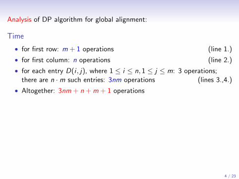
Analysis of DP algorithm for global alignment:

Time

• for first row: m + 1 operations (line 1.)

• for first column: n operations (line 2.)

• for each entry D(i , j), where 1 ≤ i ≤ n, 1 ≤ j ≤ m: 3 operations;there are n ·m such entries: 3nm operations (lines 3.,4.)

• Altogether: 3nm + n + m + 1 operations

Space

• matrix of size (n + 1)(m + 1) = nm + n + m + 1 entries (units)

Equal length strings

If n = m then time = 3n2 + 2n + 1, space = n2 + 2n + 1

4 / 23

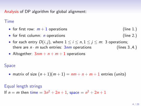
Let’s compare this with the other algorithm we saw for global alignment:

Exhaustive search

1. consider every possible alignment of s and t

2. for each of these, compute its score

3. output the maximum of these

5 / 23

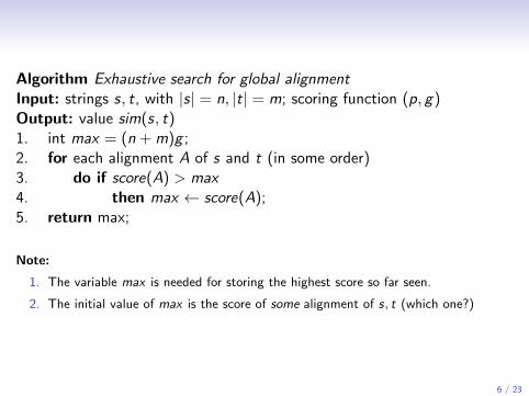
Algorithm Exhaustive search for global alignmentInput: strings s, t, with |s| = n, |t| = m; scoring function (p, g)Output: value sim(s, t)1. int max = (n + m)g ;2. for each alignment A of s and t (in some order)3. do if score(A) > max4. then max ← score(A);5. return max;

Note:

1. The variable max is needed for storing the highest score so far seen.

2. The initial value of max is the score of some alignment of s, t (which one?)

6 / 23

Analysis of Exhaustive search:

• Time: next slides

• Space: exercise

7 / 23

Analysis of Exhaustive search (time):

• for every alignment (line 2.)

no. of al’s

• compute its score (line 3.)

length of al.

time = no. of alignments︸ ︷︷ ︸N(n,m)

· length of alignment︸ ︷︷ ︸between max(n,m) and n+m

Simplify analysis: Let’s look at two equal length strings |s| = |t| = n:

N(n, n) · n ≤ time ≤ N(n, n) · 2n

We have seen: N(n, n) > 2n, so time ≥ 2n · n.

8 / 23

Analysis of Exhaustive search (time):

• for every alignment (line 2.) no. of al’s

• compute its score (line 3.)

length of al.

time = no. of alignments︸ ︷︷ ︸N(n,m)

· length of alignment︸ ︷︷ ︸between max(n,m) and n+m

Simplify analysis: Let’s look at two equal length strings |s| = |t| = n:

N(n, n) · n ≤ time ≤ N(n, n) · 2n

We have seen: N(n, n) > 2n, so time ≥ 2n · n.

8 / 23

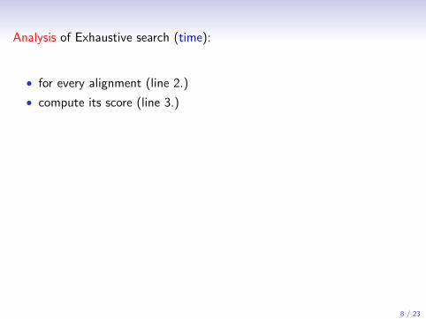
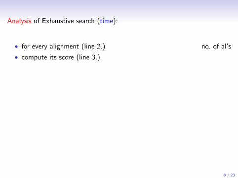
Analysis of Exhaustive search (time):

• for every alignment (line 2.) no. of al’s

• compute its score (line 3.) length of al.

time = no. of alignments︸ ︷︷ ︸N(n,m)

· length of alignment︸ ︷︷ ︸between max(n,m) and n+m

Simplify analysis: Let’s look at two equal length strings |s| = |t| = n:

N(n, n) · n ≤ time ≤ N(n, n) · 2n

We have seen: N(n, n) > 2n, so time ≥ 2n · n.

8 / 23

Analysis of Exhaustive search (time):

• for every alignment (line 2.) no. of al’s

• compute its score (line 3.) length of al.

time = no. of alignments︸ ︷︷ ︸N(n,m)

· length of alignment︸ ︷︷ ︸between max(n,m) and n+m

Simplify analysis: Let’s look at two equal length strings |s| = |t| = n:

N(n, n) · n ≤ time ≤ N(n, n) · 2n

We have seen: N(n, n) > 2n, so time ≥ 2n · n.

8 / 23

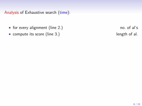
Analysis of Exhaustive search (time):

• for every alignment (line 2.) no. of al’s

• compute its score (line 3.) length of al.

time = no. of alignments︸ ︷︷ ︸N(n,m)

· length of alignment︸ ︷︷ ︸between max(n,m) and n+m

Simplify analysis: Let’s look at two equal length strings |s| = |t| = n:

N(n, n) · n ≤ time ≤ N(n, n) · 2n

We have seen: N(n, n) > 2n, so time ≥ 2n · n.

8 / 23

So we have, for |s| = |t| = n:

• DP algo: 3n2 + 2n + 1 operations

• Exhaustive search: at least N(n, n) · n operations

Let’s compare the two functions for increasing n:

n 1 2 3 4 5 . . . 10 100 10003n2 + 2n + 1 6 17 34 57 86 . . . 321 30 201 3 002 001

N(n, n) · n 3 26 189 1284 8415 . . . ≈ 80 · 106 ≈ 2 · 1077 ≈ 10700

The DP algorithm is much faster than the exhaustive search algorithm,because its running time increases much slower as the input size increases.But how much?

9 / 23

Algorithm analysis

• We measure running time and storage space, measured in no. ofoperations and no. of storage units.

• We want to know how our algo performs depending on the size of theinput (bigger input = more time/space), i.e. as functions of the inputsize (usually denoted n, m).

• We are interested in the algorithm’s behaviour for large inputs.

• We want to know the growth behaviour, i.e. how time/spacerequirements change as input increases.

• We want an upper bound, i.e. on any input how much time/spaceneeded at most? (worst-case analysis)

10 / 23

Algorithm analysis

• We measure running time and storage space, measured in no. ofoperations and no. of storage units.

• We want to know how our algo performs depending on the size of theinput (bigger input = more time/space), i.e. as functions of the inputsize (usually denoted n, m).

• We are interested in the algorithm’s behaviour for large inputs.

• We want to know the growth behaviour, i.e. how time/spacerequirements change as input increases.

• We want an upper bound, i.e. on any input how much time/spaceneeded at most? (worst-case analysis)

10 / 23

Algorithm analysis

• We measure running time and storage space, measured in no. ofoperations and no. of storage units.

• We want to know how our algo performs depending on the size of theinput (bigger input = more time/space), i.e. as functions of the inputsize (usually denoted n, m).

• We are interested in the algorithm’s behaviour for large inputs.

• We want to know the growth behaviour, i.e. how time/spacerequirements change as input increases.

• We want an upper bound, i.e. on any input how much time/spaceneeded at most? (worst-case analysis)

10 / 23

Algorithm analysis

• We measure running time and storage space, measured in no. ofoperations and no. of storage units.

• We want to know how our algo performs depending on the size of theinput (bigger input = more time/space), i.e. as functions of the inputsize (usually denoted n, m).

• We are interested in the algorithm’s behaviour for large inputs.

• We want to know the growth behaviour, i.e. how time/spacerequirements change as input increases.

• We want an upper bound, i.e. on any input how much time/spaceneeded at most? (worst-case analysis)

10 / 23

Algorithm analysis

• We measure running time and storage space, measured in no. ofoperations and no. of storage units.

• We want to know how our algo performs depending on the size of theinput (bigger input = more time/space), i.e. as functions of the inputsize (usually denoted n, m).

• We are interested in the algorithm’s behaviour for large inputs.

• We want to know the growth behaviour, i.e. how time/spacerequirements change as input increases.

• We want an upper bound, i.e. on any input how much time/spaceneeded at most? (worst-case analysis)

10 / 23

Consider 3 algorithms A,B, C:

input size nrunning t. 10 20 What happened when input doubled?

A n 10

20 doubled

B n2 100

400 quadrupled

C 2n 1024

1 048 576 squared

Now 3 algorithms A′,B′, C′:

input size nrunning t. 10 20 What happened when input doubled?

A′ 3n 30 60B′ 3n2 300 1200C′ 3 · 2n 3072 3 145 728

11 / 23

Consider 3 algorithms A,B, C:

input size nrunning t. 10 20 What happened when input doubled?

A n 10 20

doubled

B n2 100 400

quadrupled

C 2n 1024 1 048 576

squared

Now 3 algorithms A′,B′, C′:

input size nrunning t. 10 20 What happened when input doubled?

A′ 3n 30 60B′ 3n2 300 1200C′ 3 · 2n 3072 3 145 728

11 / 23

Consider 3 algorithms A,B, C:

input size nrunning t. 10 20 What happened when input doubled?

A n 10 20 doubledB n2 100 400

quadrupled

C 2n 1024 1 048 576

squared

Now 3 algorithms A′,B′, C′:

input size nrunning t. 10 20 What happened when input doubled?

A′ 3n 30 60B′ 3n2 300 1200C′ 3 · 2n 3072 3 145 728

11 / 23

Consider 3 algorithms A,B, C:

input size nrunning t. 10 20 What happened when input doubled?

A n 10 20 doubledB n2 100 400 quadrupledC 2n 1024 1 048 576

squared

Now 3 algorithms A′,B′, C′:

input size nrunning t. 10 20 What happened when input doubled?

A′ 3n 30 60B′ 3n2 300 1200C′ 3 · 2n 3072 3 145 728

11 / 23

Consider 3 algorithms A,B, C:

input size nrunning t. 10 20 What happened when input doubled?

A n 10 20 doubledB n2 100 400 quadrupledC 2n 1024 1 048 576 squared

Now 3 algorithms A′,B′, C′:

input size nrunning t. 10 20 What happened when input doubled?

A′ 3n 30 60B′ 3n2 300 1200C′ 3 · 2n 3072 3 145 728

11 / 23

Consider 3 algorithms A,B, C:

input size nrunning t. 10 20 What happened when input doubled?

A n 10 20 doubledB n2 100 400 quadrupledC 2n 1024 1 048 576 squared

Now 3 algorithms A′,B′, C′:

input size nrunning t. 10 20 What happened when input doubled?

A′ 3n 30 60B′ 3n2 300 1200C′ 3 · 2n 3072 3 145 728

11 / 23

Consider 3 algorithms A,B, C:

input size nrunning t. 10 20 What happened when input doubled?

A n 10 20 doubledB n2 100 400 quadrupledC 2n 1024 1 048 576 squared

Now 3 algorithms A′,B′, C′:

input size nrunning t. 10 20 What happened when input doubled?

A′ 3n 30 60 doubledB′ 3n2 300 1200 quadrupledC′ 3 · 2n 3072 3 145 728 1/3 of squared

11 / 23

The O-notation allows us to abstract from constants (3n vs. n) and otherdetails which are not important for the growth behaviour of functions.

Definition (O-classes)

Given a function f : N→ R, then O(f (n)) is the class (set) of functionsg(n) s.t.:

There exists a c > 0 and an n0 ∈ N s.t. for all n ≥ n0: g(n) ≤ c · f (n).

We then say that

g(n) ∈ O(f (n)) or g(n) = O(f (n))︸ ︷︷ ︸Careful, this is not an ”equality”!

Meaning: “g is smaller or equal than f (w.r.t. growth behaviour)”“g does not grow faster than f ”

12 / 23

The O-notation allows us to abstract from constants (3n vs. n) and otherdetails which are not important for the growth behaviour of functions.

Definition (O-classes)

Given a function f : N→ R, then O(f (n)) is the class (set) of functionsg(n) s.t.:

There exists a c > 0 and an n0 ∈ N s.t. for all n ≥ n0: g(n) ≤ c · f (n).

We then say that

g(n) ∈ O(f (n)) or g(n) = O(f (n))︸ ︷︷ ︸Careful, this is not an ”equality”!

Meaning: “g is smaller or equal than f (w.r.t. growth behaviour)”“g does not grow faster than f ”

12 / 23

The O-notation allows us to abstract from constants (3n vs. n) and otherdetails which are not important for the growth behaviour of functions.

Definition (O-classes)

Given a function f : N→ R, then O(f (n)) is the class (set) of functionsg(n) s.t.:

There exists a c > 0 and an n0 ∈ N s.t. for all n ≥ n0: g(n) ≤ c · f (n).

We then say that

g(n) ∈ O(f (n)) or g(n) = O(f (n))︸ ︷︷ ︸Careful, this is not an ”equality”!

Meaning: “g is smaller or equal than f (w.r.t. growth behaviour)”“g does not grow faster than f ”

12 / 23

Example

3n2 + 2n + 1 ∈ O(n2)

Recall definitiong(n) ∈ O(f (n)) ifthere exists a c > 0 and an n0 ∈ N s.t. for all n ≥ n0: g(n) ≤ c · f (n).

Proof

Choose c = 4 and n0 = 3. We have: ∀n ≥ 3 : 3n2 + 2n + 1 ≤ 4n2.

n 1 2 3 4 53n2 + 2n + 1 6 17 34 57 86

4n2 4 16 36 64 100

3n2 + 2n + 1 ≤ 4n2

⇔ n2 − 2n − 1 ≥ 0

⇔ (n − 1)2 − 2 ≥ 0

⇔ (n − 1)2 ≥ 2

⇔ n ≥ 3

13 / 23

Example

3n2 + 2n + 1 ∈ O(n2)

Recall definitiong(n) ∈ O(f (n)) ifthere exists a c > 0 and an n0 ∈ N s.t. for all n ≥ n0: g(n) ≤ c · f (n).

Proof

Choose c = 4 and n0 = 3. We have: ∀n ≥ 3 : 3n2 + 2n + 1 ≤ 4n2.

n 1 2 3 4 53n2 + 2n + 1 6 17 34 57 86

4n2 4 16 36 64 100

3n2 + 2n + 1 ≤ 4n2

⇔ n2 − 2n − 1 ≥ 0

⇔ (n − 1)2 − 2 ≥ 0

⇔ (n − 1)2 ≥ 2

⇔ n ≥ 3

13 / 23

Example

3n2 + 2n + 1 ∈ O(n2)

Recall definitiong(n) ∈ O(f (n)) ifthere exists a c > 0 and an n0 ∈ N s.t. for all n ≥ n0: g(n) ≤ c · f (n).

Proof

Choose c = 4 and n0 = 3. We have: ∀n ≥ 3 : 3n2 + 2n + 1 ≤ 4n2.

n 1 2 3 4 53n2 + 2n + 1 6 17 34 57 86

4n2 4 16 36 64 100

3n2 + 2n + 1 ≤ 4n2

⇔ n2 − 2n − 1 ≥ 0

⇔ (n − 1)2 − 2 ≥ 0

⇔ (n − 1)2 ≥ 2

⇔ n ≥ 3

13 / 23

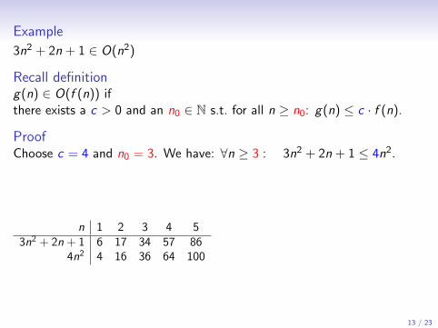
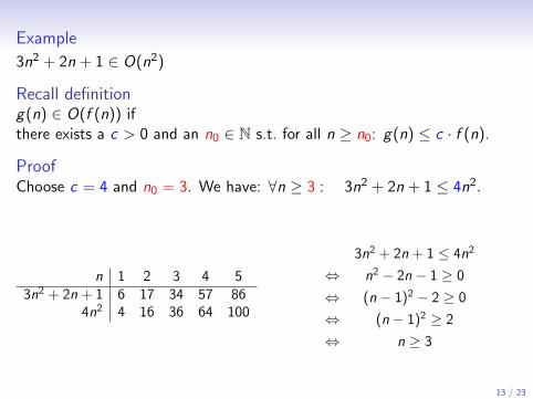
Example

3n2 + 2n + 1 ∈ O(n2)

Recall definitiong(n) ∈ O(f (n)) ifthere exists a c > 0 and an n0 ∈ N s.t. for all n ≥ n0: g(n) ≤ c · f (n).

ProofChoose c = 4 and n0 = 3. We have: ∀n ≥ 3 : 3n2 + 2n + 1 ≤ 4n2.

n 1 2 3 4 53n2 + 2n + 1 6 17 34 57 86

4n2 4 16 36 64 100

3n2 + 2n + 1 ≤ 4n2

⇔ n2 − 2n − 1 ≥ 0

⇔ (n − 1)2 − 2 ≥ 0

⇔ (n − 1)2 ≥ 2

⇔ n ≥ 3

13 / 23

Example

3n2 + 2n + 1 ∈ O(n2)

Recall definitiong(n) ∈ O(f (n)) ifthere exists a c > 0 and an n0 ∈ N s.t. for all n ≥ n0: g(n) ≤ c · f (n).

ProofChoose c = 4 and n0 = 3. We have: ∀n ≥ 3 : 3n2 + 2n + 1 ≤ 4n2.

n 1 2 3 4 53n2 + 2n + 1 6 17 34 57 86

4n2 4 16 36 64 100

3n2 + 2n + 1 ≤ 4n2

⇔ n2 − 2n − 1 ≥ 0

⇔ (n − 1)2 − 2 ≥ 0

⇔ (n − 1)2 ≥ 2

⇔ n ≥ 3

13 / 23

3n2 + 2n + 1 ∈ O(n2): ∀n ≥ 3 : 3n2 + 2n + 1 ≤ 4n2

plot: WolframAlpha 14 / 23

plot: WolframAlpha

15 / 23

plot: WolframAlpha

16 / 23

In practice:

• identify which input parameters are important—no. months n forFibonacci numbers; length of strings n,m for pairwise al.

• order additive terms according to these in decreasing growth order:3n5 + 2n3 + n + 7,3nm + n + m + 1

• take largest without multiplicative constant:3n5 + 2n3 + n + 7 ∈ O(n5),3nm + n + m + 1 ∈ O(nm)

17 / 23

Important O-classes

The most important functions, ordered by increasing O–classes: each function fiis in the O–class of the next function fi+1, but fi+1(n) /∈ O(fi (n)).

1 log log n log n√n n n log n n2 n3 . . . . . . 2n n! nn

cons- loga- linear quad- cubic expo-tant rith- ratic nen-

mic tialpolynomial (of the form nc for some constant c)

(all except n log n are polynomials)E F F I C I E N T1 inefficient

function grows slower ←→ function grows fasterfaster algorithm slower algorithm

1also called feasible vs. infeasible18 / 23

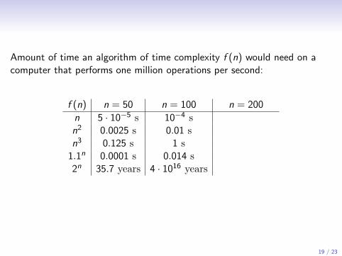
Amount of time an algorithm of time complexity f (n) would need on acomputer that performs one million operations per second:

f (n) n = 50 n = 100 n = 200

n 5 · 10−5 s 10−4 s

2 · 10−4 s

n2 0.0025 s 0.01 s

0.04 s

n3 0.125 s 1 s

8 s

1.1n 0.0001 s 0.014 s

190 s

2n 35.7 years 4 · 1016 years

5 · 1046 years

19 / 23

Amount of time an algorithm of time complexity f (n) would need on acomputer that performs one million operations per second:

f (n) n = 50 n = 100 n = 200

n 5 · 10−5 s 10−4 s 2 · 10−4 sn2 0.0025 s 0.01 s 0.04 sn3 0.125 s 1 s 8 s

1.1n 0.0001 s 0.014 s 190 s2n 35.7 years 4 · 1016 years 5 · 1046 years

19 / 23

On a 1000 times faster computer:

f (n) n = 50 n = 100 n = 200

n 5 · 10−8 s 10−7 s 2 · 10−7 sn2 2.5 · 10−6 s 10−5 s 4 · 10−5 sn3 1.25 · 10−4 s 10−3 s 8 · 10−3 s

1.1n 1.1 · 10−7 s 1.4 · 10−5 s 0.19 s2n 13 days 4 · 1013 years 5 · 1043 years

20 / 23

Looking at it in a different way . . .

1 2 3 4 5 . . . 10 20 100 1000 106

n 1 2 3 4 5 . . . 10 20 100 1000 106

n2 1 4 9 16 25 . . . 100 400 10000 106

2n 2 4 8 16 32 . . . 1024 ≈ 106 ≈ 1030 ≈ 10301

On a computer that can perform one million operations per second, in asecond,

• a linear-time algorithm can solve a problem instance of size 106 (onemillion) (e.g. fib2, fib3),

• a quadratic-time algorithm one of size 1000 (one thousand),

• an exponential-time algorithm one of size 20 (e.g. fib1).

In fact, on any computer, these algorithms need always the same amountof time for problem instances of such different sizes!

21 / 23

Looking at it in a different way . . .

1 2 3 4 5 . . . 10 20 100 1000 106

n 1 2 3 4 5 . . . 10 20 100 1000 106

n2 1 4 9 16 25 . . . 100 400 10000 106

2n 2 4 8 16 32 . . . 1024 ≈ 106 ≈ 1030 ≈ 10301

On a computer that can perform one million operations per second, in asecond,

• a linear-time algorithm can solve a problem instance of size 106 (onemillion) (e.g. fib2, fib3),

• a quadratic-time algorithm one of size 1000 (one thousand),

• an exponential-time algorithm one of size 20 (e.g. fib1).

In fact, on any computer, these algorithms need always the same amountof time for problem instances of such different sizes!

21 / 23

Back to the global alignment algorithms:

• A(n) := 3n2 + 2n + 1 running time of DP algo

• B(n) := n · N(n, n) running time of exhaustive search algo

1 2 3 4 5 . . . 10 20 100 1000A(n) 6 17 34 57 86 . . . 321 1241 30 201 3 002 001B(n) 3 26 189 1284 8415 . . . ≈ 80 · 106 ≈ 5 · 1016 ≈ 2 · 1077 ≈ 10700

n 1 2 3 4 5 . . . 10 20 100 1000n2 1 4 9 16 25 . . . 100 400 10 000 106

2n 2 4 8 16 32 . . . 1024 ≈ 106 ≈ 1030 ≈ 10301

• A(n) ∈ O(n2) a quadratic time algorithm

• B(n) is super-exponential

22 / 23

Analysis of our alignment algorithms

algorithm time space

DP for global alignment, only sim(s, t) O(nm) O(nm)[equal length strings O(n2) O(n2)]

computing an optimal alignment O(n + m) none1

[equal length strings O(n) none1]

space saving variant of DP for O(nm) O(min(n,m))global alignment, only sim(s, t)

[equal length strings O(n2) O(n)]

DP for local alignment O(nm) O(nm)[equal length strings O(n2) O(n2)]

1assuming the O(n2) size DP-table is given23 / 23