Algorithms for Sparse Non-negative Tucker

decompositions

Morten Mørup and Lars Kai HansenTechnical University of Denmark, 2800 Kongens Lyngby, Denmark

Sidse M. ArnfredDepartment of Psychiatry, Hvidovre hospital, University Hospital of Copenhagen,

Denmark

Abstract There is a increasing interest in analysis of largescale multi-way data. The concept of multi-way data refersto arrays of data with more than two dimensions, i.e., tak-ing the form of tensors. To analyze such data, decompo-sition techniques are widely used. The two most commondecompositions for tensors are the Tucker model and themore restricted PARAFAC model. Both models can beviewed as generalizations of the regular factor analysisto data of more than two modalities. Non-negative ma-trix factorization (NMF) in conjunction with sparse cod-ing has lately been given much attention due to its partbased and easy interpretable representation. While NMFhas been extended to the PARAFAC model no such at-tempt has been done to extend NMF to the Tucker model.However, if the tensor data analyzed is non-negative itmay well be relevant to consider purely additive (i.e.,non-negative Tucker decompositions). To reduce ambi-guities of this type of decomposition we develop updatesthat can impose sparseness in any combination of modal-ities, hence, proposed algorithms for sparse non-negativeTucker decompositions (SN-TUCKER). We demonstratehow the proposed algorithms are superior to existing al-gorithms for Tucker decompositions when indeed the dataand interactions can be considered non-negative. We fur-ther illustrate how sparse coding can help identify whatmodel (PARAFAC or Tucker) is the most appropriate forthe data as well as to select the number of componentsby turning o� excess components. The algorithms for SN-

TUCKER can be downloaded from [Mørup, 2007].

1 Introduction

Tensor decompositions are in frequent use today in a variety of�elds including psychometric, chemometrics, image analysis, graphanalysis and signal processing [Murakami and Kroonenberg, 2003;Vasilescu and Terzopoulos, 2002; Wang and Ahuja, 2003; Jia andGong, 2005; Sun et al., 2005; Gurden et al., 2001; Nørgaard andRidder, 1994; Smilde et al., 1999, 2004; Andersson and Bro, 1998].Tensors, i.e., X ∈ <I1×I2×...×IN , also called multi-way arrays or mul-tidimensional matrices are generalizations of vectors (�rst order ten-sors) and matrices (second order tensors). The two most commonlyused decompositions of tensors are the Tucker model [Tucker, 1966]and the more restricted PARAFAC/CANDECOMP model [Harsh-man, 1970; Carroll and Chang, 1970].

The Tucker model reads

Xi1,i2,...,iN ≈ Ri1,i2,...,iN =∑

j1j2...jN

Gj1,j2,...,jNA(1)i1,j1

A(2)i2,j2·...·A(N)

iN ,jN. (1)

where G ∈ <J1×J2×...×JN and A(n) ∈ <In×Jn . To indicate how manyvectors pertain to each modality it is customary also to denote themodel a Tucker J1−J2−· · ·−JN . Using the n-mode tensor product×n [Lathauwer et al., 2000] given by

(Q×n P)i1,i2,...,jn,...iN =∑in

Qi1,i2,...,in,...iNPjn,in , (2)

the model is stated as

X ≈ R = G ×1 A(1) ×2 A(2) ×3 ...×N A(N). (3)

The Tucker model represents the data spanning the nth modality bythe vectors (loadings) given by the Jn columns of A(n) such that thevectors of each modality interact with the vectors of all remainingmodalities with strengths given by a so-called core tensor G. As aresult, the Tucker model encompass all possible linear interactionsbetween vectors pertaining to the various modalities of the data.

2

The PARAFAC model is a special case of the Tucker model wherethe size of each modality of the core array G is the same, i.e., J1 =J2 = · · · = JN while interaction is only between columns of sameindices such that the only non-zero elements are found along thediagonal of the core, i.e., Gj1,j2,...,jN 6= 0 i� j1 = j2 = ... = jN .Notice, in the Tucker model a rotation of a given loading matrix A(n)

can be compensated by a counter rotation of the core G, i.e., G ×nA(n) = (G×nP−1)×n(A(n)P). While the factors of the unconstrainedTucker model are orthogonal, this is not the case for the factors of thePARAFAC model. Furthermore, as the PARAFAC model requiresthe core to be diagonal this restricts P in general to be a simple scaleand permutation matrix. Thus, contrary to the PARAFAC model[Kruskal, 1977; Sidiropoulos and Bro, 2000] the Tucker model is notunique in general.

Non-negative matrix factorization (NMF) is given by the decom-position

V ≈ R = WH, (4)

where V ∈ <N×M+ , W ∈ <N×D+ and H ∈ <D×M+ , i.e., such that thevariables V, W and H are non-negative. The decomposition is use-ful as it results in easy interpretable part based representations [Leeand Seung, 1999]. Non-negative decomposition is also named positivematrix factorization [Paatero and Tapper, 1994] but was popularizedby Lee and Seung [1999, 2000] due to a simple and e�cient algorith-mic procedure based on multiplicative updates. The decompositionhas proven useful for a wide range of data where non-negativity isa natural constraint. These encompass data for text-mining basedon word frequencies, image data, biomedical data and spectral data.The algorithm can even be useful when the data inherently is in-de�nite, but after transformation becomes non-negative, say audio,where NMF has been successfully used for analysis of the amplitudeof a spectral representation [Smaragdis and Brown, 2003].

Unfortunately, the decomposition is not in general unique [Donohoand Stodden, 2003]. However, sparseness has been imposed such thatambiguities are reduced by �nding the solution being the most sparse(by some measure of sparseness). This is often also the most simple,i.e., parsimonious solution to the data [Olshausen and Field, 2004;Eggert and Körner, 2004; Hoyer, 2004]. Non-negative matrix factor-

3

ization has recently been extended to the PARAFAC model [Wellingand Weber, 2001; FitzGerald et al., 2005; Parry and Essa, 2006; Ci-chocki et al., 2007]. However, despite the attractive properties ofnon-negative decompositions and sparse coding neither approacheshave so far been extended to the Tucker model.

Traditionally, the Tucker model has been estimated using vari-ous alternating least squares algorithms where the columns of A(n)

for the unconstrained Tucker are orthogonal [Andersson and Bro,1998]. Recently, an algorithm for higher order singular value decom-position (HOSVD) based on solving N eigenvalue problems to esti-mate the Tucker model was given [Lathauwer et al., 2000]. However,just as NMF does not have orthogonal factors neither will factorsin the constrained Tucker model be forced orthogonal. Althoughalgorithms for non-negative Tucker decompositions exist [Bro andAndersson, 2000] the decompositions do not allow for the core tobe constrained non-negative. Furthermore, the decompositions arein general ambiguous. Consequently, the lack of uniqueness hampersinterpretability of these decompositions. For this reason the exist-ing non-negative Tucker decompositions have not been widely used.Presently, we will develop multiplicative algorithms for fully non-negative Tucker decompositions, i.e., forming a non-negative Tuckerdecomposition where both data, core and loadings are non-negative.Ambiguities of the decompositions are reduced imposing sparsenesssuch that the solution being the sparsest according to some measureof sparsity is attained.

In the following X ab will denote a tensor of the modalities a con-

taining data of type b. Recently, the Tucker model has among othersbeen applied to:

1. Spectroscopy data ([Smilde et al., 2004; Andersson and Bro, 1998]for instance XBatch number×T ime×Spectra

Strength [Gurden et al., 2001; Nør-gaard and Ridder, 1994; Smilde et al., 1999])

2. Web mining (X Users×Queries×Wep pagesClick counts [Sun et al., 2005])

3. Image analysis (X People×V iews×Illuminations×Expressions×PixelsImage intensity [Vasilescu

and Terzopoulos, 2002; Wang and Ahuja, 2003; Jia and Gong,2005]

4. Semantic di�erential data (X Judges×Music pieces×ScalesGrade [Murakami and

4

Kroonenberg, 2003])

All the above data sets are non-negative and the basis vectors/projectionsA(n) and interactions G can be assumed additive, viz., non-negative.For the spectroscopy data non-negativity would yield batch groupscontaining, time and spectra pro�les additively combined by the non-negative core, for the web mining data giving groups of users, queriesand web pages interrelated with a strength given by the non-negativecore etc. However, none of the Tucker analysis above have consid-ered such purely non-negative decompositions where the �whole� ismodeled as the sum of its �parts� resulting in easy interpretable partbased representation.

The paper is structured as follows: First, two algorithms for sparsenon-negative Tucker (SN-TUCKER) decomposition based on a gaus-sian noise model (i.e., least squares (LS) minimization) and Poissonnoise (i.e., Kulback-Leibler (KL) divergence minimization) are de-rived. The derivation easily generalizes to other types of objectivefunctions such as Bregman, Ciszar, α and β divergences [Dhillonand Sra, 2005; Cichocki et al., 2006, 2007], however, the focus ishere on LS and KL, since they are the two most widely used objec-tive functions for NMF. Next, the algorithms ability to identify thecomponents of synthetically generated data is demonstrated. Finally,the algorithms are tested on two real data sets, one of wavelet trans-formed EEG previously explored by the PARAFAC model [Mørupet al., 2006] the other a data set obtained from a �ow injectionanalysis (FIA) [Nørgaard and Ridder, 1994; Smilde et al., 1999].The applications demonstrate di�erent aspects of the SN-TUCKERmodel.

2 Methods

In the following A•B and ABwill denote element-wise multiplication

and division, respectively, while (M).α denotes elements-wise raisingthe elements of M to the αth power. E , E and 1 will, respectively,denote a tensor, a matrix, and a vector of ones in all entries. Finally,• supersedes · where · denotes the regular matrix multiplication.

The sparse non-negative Tucker (SN-TUCKER) algorithms pro-posed here is based on the multiplicative updates introduced in [Lee

5

and Seung, 1999, 2000; Lee et al., 2002] for non-negative matrix fac-torization (NMF). Although, other types of updates exists for non-negativity constraint optimization such as projected gradient [Lin,2007] and active sets [Bro and Jong, 1997], multiplicative updates aresimple to implement and extend well to sparse coding [Eggert andKörner, 2004]. Consider the cost function C(θ) of the non-negative

variables θ. Let further ∂C(θ)+i∂θi

and ∂C(θ)−i∂θi

be the positive and nega-tive part of the derivative with respect to θi. Then the multiplicativeupdate has the following form:

θi ← θi

(∂C(θ)−

∂θi∂C(θ)+

∂θi

)α

. (5)

A small constant ε = 10−9 can be added to the denominator to avoidpotential division by zero. By also adding the constant to the nu-merator the corresponding gradient is unaltered. When the gradient

is zero ∂C(θ)∂θi

+= ∂C(θ)−

∂θisuch that θ is left unchanged. If the gradi-

ent is positive ∂C(θ)+

∂θi> ∂C(θ)−

∂θihence θi will decrease and vice versa

if the gradient is negative. Thus, there is a one-to-one relation be-tween �xed points of the multiplicative update rule and stationarypoints under gradient descend. One attractive property of multiplica-tive updates is that, since θi,

∂C(θ)+

∂θiand ∂C(θ)−

∂θiall are non-negative,

non-negativity is naturally enforced as each update remains in thepositive orthant. α is a step size parameter that potentially can betuned to assist convergence. When α → 0 only very small steps inthe negative gradient direction are taken.

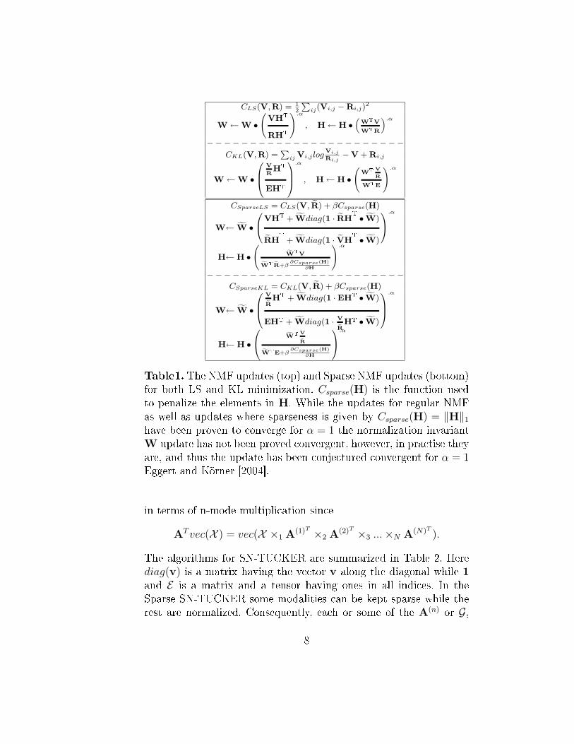
Using multiplicative updates Lee and Seung [2000] devised twoalgorithms for NMF. One based on least squares minimization (LS)corresponding to the approximation error being homoscedatic gaus-sian noise the other based on Kullback-Leibler divergence (KL) cor-responding to Poisson noise. They further proved that these updatesgiven at the top of Table 1 monotonically decrease the cost functionC for α = 1.

Although the estimation of W or H for �xed H or W, respec-tively, is a convex problem, the combined estimation alternatinglysolving for W and H is not guaranteed to �nd the global minima.Furthermore, a NMF decomposition is in general not unique [Donoho

6

and Stodden, 2003]: If the data does not adequately span the positiveorthant a rotation of the solution is possible violating uniqueness.Consequently, constraints in the form of sparseness has proven use-ful such that the ambiguity is resolved taking the solution being thesparsest by some measure of sparseness [Hoyer, 2002, 2004; Eggertand Körner, 2004]. Eggert and Körner [2004] derived an e�cient algo-rithm for Sparse NMF based on multiplicative updates by penalizingvalues in H by a function Csparse(H) while keeping W normalizedsuch that the sparsity is not achieved simply by letting H go to zerowhile W goes to in�nity. Making the reconstruction invariant to thisnormalization, i.e., R = WH where Wi,d =

Wi,d√ΣiW2

i,d

=Wi,d

‖Wd‖F, they

found multiplicative updates for the LS-algorithm which can be ex-tended to the KL-algorithm, see Table 1. In the following analysis wewill use Csparse(H) = ‖H‖1, i.e., an L1-norm penalty. One attractiveproperty of the L1-norm is that it can function as a proxy for the L0

norm, i.e., can minimize the number of non-zero elements while isdoes not change the convexity of the cost-function when estimatingH for �xed W [Donoho, 2006]. Notice, ∂Csparse(H)

∂H= 1.

Consider the non-negative Tucker model, i.e X , G and A(n) areall non-negative. By 'matrizicing' X I1×I2×...×IN into a matrix, i.e.,XIn×I1...In−1In+1...IN(n) the Tucker model can be expressed in matrix no-

tation as [Lathauwer et al., 2000]

X(n) ≈ R(n) = A(n)G(n)(A(N) ⊗ ...⊗A(n+1) ⊗A(n−1) ⊗ ...⊗A(1)) = A(n)Z(n),

where Z(n) = G(n)(A(N) ⊗ ...⊗A(n+1) ⊗A(n−1) ⊗ ...⊗A(1))T . As a

result, the updates of each of the factors A(n) follow straightforwardfrom the regular NMF updates by exchanging W with A(n) and Hwith Z(n) in the W update.

By lexicographical indexing of the elements in X and G, i.e.,vec(X ) and vec(G) the problem of �nding the core G can be for-mulated in the framework of conventional factor analysis [Kolda,2006]:

vec(X ) ≈ vec(R) = Avec(G),

where A = A(1) ⊗A(2) ⊗ ...⊗A(N). Consequently, the update of Gfollows by the regular NMF updates exchanging W with A and Hwith vec(G) in the H update. Finally, this update can be expressed

7

CLS(V,R) = 12

∑ij(Vi,j −Ri,j)

2

W←W •

(VHT

RHT

).α, H← H •

(WTV

WTR

).α−−−−−−−−−−−−−−−−−−−−−−−

CKL(V,R) =∑ij Vi,j log

Vi,jRi,j−V + Ri,j

W←W •

V

RHT

EHT

.α

, H← H •

(WT V

R

WTE

).αCSparseLS = CLS(V, R) + βCsparse(H)

W← W •

VHT + Wdiag(1 · RHT

• W)

RHT

+ Wdiag(1 · VHT

• W)

.α

H← H •

(WTV

WTR+β∂Csparse(H)

∂H

).α−−−−−−−−−−−−−−−−−−−−−−−

CSparseKL = CKL(V, R) + βCsparse(H)

W← W •

V

RHT + Wdiag(1 ·EHT • W)

EHT + Wdiag(1 · V

RHT • W)

.α

H← H •

WT V

R

WTE+β∂Csparse(H)

∂H

.α

Table1. The NMF updates (top) and Sparse NMF updates (bottom)for both LS and KL minimization. Csparse(H) is the function usedto penalize the elements in H. While the updates for regular NMFas well as updates where sparseness is given by Csparse(H) = ‖H‖1have been proven to converge for α = 1 the normalization invariantW update has not been proved convergent, however, in practise theyare, and thus the update has been conjectured convergent for α = 1Eggert and Körner [2004].

in terms of n-mode multiplication since

ATvec(X ) = vec(X ×1 A(1)T ×2 A(2)T ×3 ...×N A(N)T ).

The algorithms for SN-TUCKER are summarized in Table 2. Herediag(v) is a matrix having the vector v along the diagonal while 1and E is a matrix and a tensor having ones in all indices. In theSparse SN-TUCKER some modalities can be kept sparse while therest are normalized. Consequently, each or some of the A(n) or G,

8

Algorithm outline for SN-TUCKER based on LS and KL minimization

1. Initialize all A(n) and the core array G for instance by random.

2. For all n do

LS-minimization:

R(n) = A(n)Z(n)

A(n) ← A(n) •(

X(n)ZT(n)

R(n)ZT(n)

).αKL-minimization:

R(n) = A(n)Z(n)

A(n) ← A(n) •

(

X(n)

R(n)

)ZT(n)

E(n)ZT(n)

.α

3. R = G ×1 A(1) ×2 A(2) ×3 ...×N A(N)

LS-minimization:

B = X ×1 A(1)T ×2 A(2)T ×3 ...×N A(N)T

C = R×1 A(1)T ×2 A(2)T ×3 ...×N A(N)T

G ← G •(BC

).αKL-minimization:

D = XR×1 A(1)T ×2 A(2)T ×3 ...×N A(N)T

F = E ×1 A(1)T ×2 A(2)T ×3 ...×N A(N)T

G ← G •(DF

).α4. Repeat from step 2 until some convergence criterion has been satis�ed

Table2. Algorithms for SN-TUCKER based on LS and KL mini-mization. In step 1, we initialized the components by random butsuch that the amplitude of the randomly generated data covered allpotential solutions by the initialization. In step 4, the convergencewas de�ned as a relative change in cost function being less than 10−6

or when the algorithm had run for 2500 iterations

can be constrained to be sparse while re-normalizing the modalitiesthat are not constrained. In conclusion, sparseness can be imposedin any combination of modalities including the core, while normal-izing the remaining modalities. In Table 2 the updates are givenwhen sparsifying or normalizing a given modality. Here ‖G‖F =√∑

j1j2....jNG2j1,j2,...,jN

that is ‖·‖F is the regular Frobenious norm for

matrices and tensors, respectively, as de�ned in [Kolda, 2006] while‖G‖1 =

∑j1j2....jN

Gj1,j2,...,jN . When normalizing, each of the updated

A(n)'s should be normalized after the update, i.e., Ain,d =Ain,d

‖Ad‖F

9

while the core is normalized by G = G‖G‖F

. Notice,

Normalized Sparse

LS A(n) •

(X(n)Z

T(n)+A(n)diag(1·R(n)Z

T(n)•A

(n))

R(n)ZT(n)+A(n)diag(1·X(n)Z

T •A(n))

).αA(n) •

(X(n)Z

T(n)

R(n)ZT(n)+β

).α

KL A(n) •

X(n)

R(n)

ZT(n)+A(n)diag(1·EZ(n)•A(n))

EZT(n)+A(n)diag(1·(

X(n)

R(n)

)ZT(n)•A

(n))

.α

A(n) •

(

X(n)

R(n)

)ZT(n)

EZT(n)+β

.α

LS G •(B+G‖C•G‖1

C+G‖B•G‖1

).αG •

(BC+β

).αKL G •

(D+G‖E•G‖1

F+G‖D•G‖1

).αG •

(DF+β

).αTable3. Updates when normalizing or imposing sparseness on thevarious modalities. Top row updates of A(n), bottom row updates ofthe core G

CLS(X(1),R(1)) = ... = CLS(X(N),R(N)) = CLS(vec(X ),Avec(G))CKL(X(1),R(1)) = ... = CKL(X(N),R(N)) = CKL(vec(X ),Avec(G)).

Each of the updates above minimize the same cost function. As aresult, the convergence of the algorithms for SN-TUCKER with-out sparseness for α = 1 follow straightforward from the conver-gence of the regular NMF updates given in [Lee and Seung, 2000] asthe estimation takes the form of a sequence of regular factor anal-ysis problems minimizing the same cost function. However, no suchproof exists for updates for normalized variables [Eggert and Körner,2004]. Although extensively tested we never experienced any lack ofconvergence of the updates above for the normalized variables forα = 1. Had the updates diverged α could have been tuned to ensureconvergence.

The proposed algorithms for SN-TUCKER are based on multi-plicative updates and in summary have the following bene�ts

� The developed algorithms can reduce ambiguities of the non-negative decompositions by imposing sparseness in any combi-nation of modalities.

10

� The non-negativity ensures that no cancellation is allowed andthat the representations becomes part based [Lee and Seung,1999]. This also often leads to clustering of the data [Ding et al.,2005].

� Overcomplete representations can be handled, for instance thecore tensor can for some modalities be much larger than the orig-inal data tensor, while sparsity can help to avoid an over�t of thedata.

� The updates can easily be adapted to consider only the non-zero elements in X reducing computational complexity for highlysparse data.

� The updates can enforce speci�c prior structure in the core or theloadings. For instance the core or some of the core elements canbe �xed to implement known interactions in the model simply byomitting the updates for these speci�c elements.

� Missing data is often a problem, however missing values can behandled by introducing an indicator tensor Q of same size as Vhaving ones where data is present and zeros where missing asdemonstrated for regular NMF in [Zhang et al., 2006]. ReplacingX by Q•X(n), R with Q•R and E with Q in the updates abovethe in�uence of missing values are completely removed in themodel estimation.

� Each iteration of the SN-TUCKER is O(I1I2 · ... ·INJ1J2 · ... ·JN),i.e., grows linearly with the product of the size of X and G mak-ing the cost per iteration relatively limited compared to existingalgorithms for non-negative TUCKER decomposition. Alterna-tive algorithms, e.g., require an iterative check of the violation ofnon-negativity [Bro and Andersson, 2000; Bro and Jong, 1997].

A drawback compared to the algorithm for non-negative constrainedoptimization such as [Bro and Jong, 1997] is that convergence canbe slow, especially for small values of the regularization parametersβ. Although the estimation of each variable in turn is a convex op-timization problem, alternatingly solving for the components of the

11

various modalities is a non-convex problem. Thus, just as for regu-lar NMF the SN-TUCKER is prone to local minima. To speed upthe convergence, we have used overrelaxed bound optimization asproposed for regular NMF in Salakhutdinov et al. [2003].

Finally, we note that if we force the core to be the identity tensorthe algorithm reduces to the algorithm for non-negative PARAFACalso named Positive Tensor Factorization (PTF) proposed in [Wellingand Weber, 2001].

3 Results and Discussion

In the following Standard Tucker will denote the algorithm for Tuckerestimation provided by the N-way toolbox Bro and Andersson [2000]while HOSVD corresponds to the Tucker algorithm described inLathauwer et al. [2000]. Furthermore, convergence will be de�nedhere as a relative change in cost function being less than 10−6 orwhen the algorithm has run for 2500 iterations.

The algorithms were �rst tested on a synthetic data set consist-ing of 5 images of logical operators mixed through two modalities.The data was generated such that a perfect non-negative decompo-sition was ambiguously de�ned. The result of the decomposition ofthe synthetic data can be seen in Figure 1. While the SN-TUCKERKL and LS algorithm near perfectly identi�es all components thecorresponding non-negative PARAFAC decomposition, with its di-agonal restriction on the core, fails in identifying the components. Forthe PARAFAC model the true interactions between the componentsof the various modalities can not be accounted for. The StandardTucker algorithm provided by the N-way toolbox also failed in esti-mating the correct components as non-negativity of the core in thecurrent implementation of the toolbox was not implemented. Thus, ifthe core is not constrained although the interactions (core-elements)are non-negative the decomposition results in an erroneous decom-position of the data. Namely, a pattern results with signi�cant can-cellation e�ects in the core that account for the data in a randomway. Thus, even though the correct model has both non-negativeloadings and interactions an unconstrained core will resort to can-cellation e�ect in order to account for the data which hampers theinterpretability of the model.

12

Figure1. Examples of results obtained when analyzing a syntheticdata set generated from a Tucker 5-5-5 model. Top left panel: Thetrue components generating the synthetic data. Top middle panel:

Components obtained by the SN-TUCKER algorithm based on KL.Top right panel: Components obtained by the SN-TUCKER al-gorithm based on LS. Bottom left panel: Components obtainedby the corresponding non-negative PARAFAC model based on KL.Bottom middle panel: Components obtained by the correspond-ing non-negative PARAFAC model based on LS. Bottom right

panel: Components obtained by the Standard Tucker algorithm pro-vided by the N-way toolbox (which is based on least squares mini-mization) allowing for the loadings to be constrained non-negativebut keeping the core unconstrained. All decompositions except thePARAFAC decomposition accounts for more than 99.99% of the vari-ance.

13

The algorithms were next tested on a data set containing theinter trial phase coherence (ITPC) obtained from wavelet trans-formed electroencephalographic (EEG) data. This data set has pre-viously been analyzed using non-negative PARAFAC and a detaileddescription of the data set can be found in [Mørup et al., 2006].Brie�y stated it consist of 14 subject recorded during a propri-oceptive stimuli consisting of a weight change of left hand dur-ing odd trials and right hand during even trials giving a total of14 · 2 = 28 trials. Consequently, the data has the following formXChannel×T ime−Frequency×TrialsITPCvalue . The results of a Tucker 3-3-3 model

can be seen in Figure 2 while an evaluation of the uniqueness of thedecompositions is given in Table 4. Clearly, the SN-TUCKER modelapproaches the non-negative PARAFAC model as sparseness is im-posed on the Core, see Figure 2. While the SN-TUCKER accountsfor 49.3 % of the variance, the sparse SN-TUCKER accounts for49.11 % of the variance whereas the non-negative PARAFAC modelaccounts for 48.9 % of the variance. Finally, the HOSVD accounts for58.9 % of the variance while the two Standard Tucker decompositionsboth accounts for around 60 % of the variance. The decompositionsconstrained to be fully non-negative are easier to interpret comparedto the HOSVD and decompositions based on Standard Tucker. Thesparse SN-TUCKER and the PARAFAC decompositions are verysimilar both indicating a right sided and left sided activity in the�rst two components primarily during odd and even trials, respec-tively, corresponding to an activity contralateral to the stimulus side.The left and right sided activity represents information processing inthe somatosensory and motor cortex situated in the parietal regionof the brain contralateral to the stimulus side such that left handis represented in the right hemisphere and vice versa for the righthand, see also [Mørup et al., 2006] for additional interpretation.

Since sparseness imposed on the core resulted in a decompositionresembling the corresponding PARAFAC decomposition we concludethat the PARAFAC rather than the full Tucker model can be con-sidered a reasonable model to the data. Consequently, the Tuckermodel with sparsity imposed on the core can help to decide whethera PARAFAC or a Tucker model is the most appropriate model fora data set. Although, the decompositions obtained by the HOSVDand the standard Tucker procedure in the N-way toolbox accounts

14

for more variance since cancellation of factors are allowed, the de-compositions are again harder to interpret. While the last factor inthe trial modality clearly di�erentiates between left and right sidestimulation and the second and third scalp components di�erentiatesbetween frontal parietal and left right activity the interpretation ofthe interactions between these components are di�cult to resolvefrom the complex pattern of interaction given by the cores. Conse-quently, although the SN-TUCKER model accounts for slightly lessof the variance it is from an interpretation point of view more at-tractive. The SN-TUCKER is given for the LS minimization sincethis is the cost function the HOSVD and the Standard Tucker arebased on.

β 0 1 10 100

LS

Channel :F1 : 0.7416±0.2990

(0.3743±0.1352)F2 : 0.8453±0.1032

(0.3328±0.0897)F3 : 0.8401±0.0945

(0.3976±0.0814)

Time − Frequency :F1 : 0.8906±0.1937

(0.3175±0.0867)F2 : 0.9317±0.0716

(0.3077±0.0674)F3 : 0.9313±0.0729

(0.3126±0.0851)

Trials :F1 : 0.9268±0.0910

(0.4050±0.1131)F2 : 0.9538±0.0480

(0.4055±0.1215)F3 : 0.8661±0.1609

(0.4835±0.0965)

Core :0.7420±0.1048

(0.2853±0.1776)

Explained variance :0.4912±0.0027

Channel :F1 : 0.9464±0.0471

(0.3427±0.0949)F2 : 0.9492±0.0541

(0.3932±0.1072)F3 : 0.9595±0.0381

(0.3660±0.1116)

Time − Frequency :F1 : 0.9753±0.0212

(0.3111±0.0378)F2 : 0.9258±0.1254

(0.3108±0.0378)F3 : 0.9368±0.1312

(0.3277±0.0484)

Trials :F1 : 0.9657±0.0222

(0.3465±0.1702)F2 : 0.9585±0.1485

(0.4852±0.0674)F3 : 0.9664±0.1161

(0.4620±0.0674)

Core :0.9139±0.0383

(0.2793±0.1244)

Explained variance :0.4909±0.0017

Channel :F1 : 1.000±0.000

(0.3813±0.1400)F2 : 1.000±0.000

(0.3636±0.1631)F3 : 1.000±0.000

(0.3417±0.1072)

Time − Frequency :F1 : 1.000±0.000

(0.2812±0.0380)F2 : 1.000±0.000

(0.3259±0.0661)F3 : 1.000±0.000

(0.3329±0.0555)

Trials :F1 : 1.000±0.000

(0.4268±0.1402)F2 : 1.000±0.000

(0.3897±0.1815)F3 : 1.000±0.000

(0.3947±0.1375)

Core :0.6963±0.3535

(0.3473±0.1470)

Explained variance :0.3695±0.0000

Channel :F1 : 1.000±0.000

(0.3428±0.1195)F2 : 1.000±3.4700.000

(0.3657±0.1406)F3 : 1.000±3.3870.000

(0.3914±0.1305)

Time − Frequency :F1 : 1.000±0.000

(0.3327±0.0398)F2 : 1.000±0.000

(0.3288±0.0417)F3 : 1.000±0.000

(0.2935±0.0210)

Trials :F1 : 1.000±0.000

(0.3681±0.0972)F2 : 1.000±0.000

(0.4116±0.1434)F3 : 1.000±0.000

(0.4507±0.1347)

Core :0.3561±0.1493

(0.3094±0.1141)

Explained variance :−0.2600±0.0000

Table4.Mean correlation between the factors of 10 runs (stopped af-ter 250 iterations) with sparseness imposed on the core array rangingfrom 0 to 100 here given for LS (range of data [0; 0.4]). In parenthesisare the correlations obtained by random (estimated by permutatingthe indices of the factors and calculating their correlation). Clearlyimposing sparseness improves uniqueness (correlation between eachdecomposition) however if the sparseness imposed on the core is toostrong all factors becomes identical only capturing the mean activ-ity while the core is arbitrary due to the identical factors). The KLalgorithm gave similar results.

15

From Table 4 we learn that each unconstrained SN-TUCKER de-composition is only inter-run correlated by about 70-90%. However,when imposing sparseness on the core a more unique decompositionwas indeed achieved hence a correlation well above 90% betweenthe components of the factors and core of the 10 decompositionswhile only slightly a�ecting the explained variance. However, by fur-ther increasing sparseness on the Core a new biased type of solutionemerged in which a mean activity is represented in all the compo-nents. Consequently, the factors were all perfectly correlated to eachother while the core could be arbitrarily chosen as long as the sum ofthe core elements remained the same leading to a high variant coreand a useless decomposition.

Finally, the algorithms were tested on a data set of X Spectra×T ime×BatchStrength

obtained from a �ow injection analysis (FIA) system, see [Nørgaardand Ridder, 1994; Smilde et al., 1999]. The data set has been an-alyzed through various supervised models using among other theprior knowledge of the concentration in each batch [Nørgaard andRidder, 1994; Smilde et al., 1999]. However, here we employ a sparseSN-TUCKER to see if this algorithm can capture the underlyingstructure in the data unsupervised. Sparseness was imposed on boththe core and batch modality (β = 0.5, range of data [0;0.637]). Theresults of the sparse Tucker 6-6-6 decomposition are given in Figure3

From the analysis of the FIA data a highly consistent decom-position resulted when imposing sparseness on the core and batchmodality, see Table 5. Here, the model captured the known true con-centrations in the batch quite well while forming a sparse core alsoimproved the interpretability of the components since less interac-tions were included, see Figure 3. Consequently, imposing sparsenesscan turn o� excess factors, hence, assist model selection also cap-turing the true loadings as presently demonstrated by the decom-positions ability to well estimate the known mixing pro�les of thebatches. Neither the decompositions without sparsity nor the Tuckerprocedure given in N-way toolbox allowing for negative core ele-ments were as consistent nor were they able to capture well the truemixing. Furthermore, the corresponding 6 component non-negativePARAFAC decomposition was not able to identify the correct mix-ing as the model was inadequate for the data. Instead it seems that

16

SN-TUCKER (β = 0) SN-TUCKER (β = 0.5) Standard TUCKER PARAFAC

mean correlation(core and loadings)

0.8986 ± 0.0722(0.3672 ± 0.1617)

0.9847 ± 0.0396(0.4008 ± 0.1736)

0.9111 ± 0.0409(0.3735 ± 0.1520)

0.9882 ± 0.0336(0.4087 ± 0.1672)

mean correlation(est. and true mixing)

0.7588 ± 0.1460(0.2984 ± 0.1979)

0.9550 ± 0.0648(0.3258 ± 0.1863)

0.5478 ± 0.0870(0.2387 ± 0.1963)

0.9391 ± 0.1032(0.2648 ± 0.1814)

explained variance 0.9995 ± 1e−5 0.9972 ± 0.0007 0.9997 ± 2e−7 0.9989 ± 4e−4

Table5. Mean correlation of 10 decompositions of the FIA datasetfor SN-TUCKER with and without sparseness as well as the Stan-dard Tucker method and non-negative PARAFAC decomposition.In parenthesis are the correlations obtained by random (estimatedby permutating the indices of the factors and calculating their cor-relation). Clearly, imposing sparseness improves component identi-�cation and reduce decomposition ambiguity while not hamperingthe models ability to account for the data. Correlation between esti-mated and true mixing is taken as the mean of the maximum corre-lation between each estimated component and the true components.

component 1 of the mixing matrix of the SN-TUCKER somewhathas been split into component 2 and 4, component 2 into 5 and 6 andcomponent 3 into component 1 and 3 of the PARAFAC decomposi-tion. Thus, the PARAFAC model is due to the restricted core forcedto split the components of one mode that are shared by several com-ponents in another mode into duplicates of the same components.That the mixing components are duplicated in the PARAFAC de-composition can also be seen from the relative high correlation of thePARAFAC model to the true mixing as given in table 5. Thus, theSN-TUCKER model yield a more compact representation than thecorresponding PARAFAC decomposition while imposing sparsenessenables to capture the true structure in the data in a completely un-supervised manner, rather than resorting to supervised approachesas previously done [Nørgaard and Ridder, 1994; Smilde et al., 1999].

By forcing the structure of the core to be the identity tensor, theSN-TUCKER algorithm becomes an algorithm for the estimationof the PARAFAC model. Although, the PARAFAC model in gen-eral is unique under mild conditions [Kruskal, 1977], the PARAFACmodel constrained to non-negativity is not in general unique [Limand Golub, 2006]. Thus, imposing sparseness as presently proposedcan also be used to alleviate the non-uniqueness of non-negativePARAFAC decompositions. The proposed SN-TUCKER has two

17

drawbacks. Estimating a good value of β is not obvious. Presently,we examined a few di�erent values of β. Future work should inves-tigate methods that more systematically estimate the β parameterssuch as approaches based on the L-curve [Hansen, 1992; Lawson andHanson, 1974], generalized cross-validation [Golub et al., 1979] orBayesian learning [Hansen et al., 2006]. Other approaches of tun-ing β have been to constrain the decompositions to give speci�cdegree of sparseness [Hoyer, 2004; Heiler and Schnörr, 2006]. How-ever, it is still not clear what degree of sparseness is desirable andas such the problem of choosing the regularization parameter β be-comes the restated problem of choosing the correct sparsity degree.That is, there is a correspondence between sparsity degree as mea-sured by 1√

InJn−1(√InJn− ‖A

(n)‖1‖A(n)‖2

) and the value of β. Furthermore,while NMF and non-negative PARAFAC normally needs in the or-der of 100 iterations to get good solutions, to our experience theSN-TUCKER needs in the order of 1000 iterations, i.e., considerablymore. The SN-TUCKER method was in general much slower thanthe HOSVD which has a closed form solution solving N eigenvalueproblems. The decomposition was also considerably slower than theStandard Tucker method provided by the N-way toolbox and thenon-negative PARAFAC proposed in [Welling and Weber, 2001].However, for both the HOSVD as well as Standard Tucker the corecan be directly calculated from pseudo-inverses of the loading ma-trices, i.e., as

G = X ×1 A(1)† ×2 A(2)† ×3 ...×N A(N)† . (6)

While for the non-negative PARAFAC no core is estimated. Thus,we also compared the present SN-TUCKER algorithm to an itera-tive procedure for fully non-negative Tucker (including non-negativecore), extending the Standard Tucker algorithm provided by the N-way toolbox to include non-negative core updates based on the ac-tive set algorithm given in [Bro and Jong, 1997]. This signi�cantlyslowed down the algorithm making it comparable in time-usage tothe SN-TUCKER algorithms we have proposed here. As a result, theSN-TUCKER model is considerably slower than Standard Tuckerand non-negative PARAFAC due to the core update. Thus, futurework should investigate how the convergence rate can be improved

18

when a closed form solution for the core no longer exists due to thenon-negativity constraints.

4 Conclusion

We proposed two new sparse non-negative Tucker (SN-TUCKER) al-gorithms. Evidence was presented that SN-TUCKER yields a partsbased representation as have been seen in NMF for 2-way data.Hence, a `simpler', more interpretable decomposition than the de-compositions obtained by current Tucker algorithms such as theHOSVD and the Standard Tucker algorithm provided by the N-waytoolbox. Furthermore, imposing constraints of sparseness helped re-duce ambiguities in the decomposition and turned o� excess compo-nents, hence helped model selection and component identi�cation.The analysis of the wavelet transformed EEG-data demonstratedhow sparseness reduced ambiguities and can further be used to iden-tify the adequacy of the PARAFAC model over the Tucker model.Whereas, the SN-TUCKER analysis of the FIA data demonstratedhow sparseness not only improve uniqueness of the decompositionsbut is also able to turn of excess components such that the true load-ings could be identi�ed unsupervised and a more compact represen-tation given than the representation obtained from the correspond-ing PARAFAC model. The algorithms presented can be downloadedfrom [Mørup, 2007].

References

Andersson, C. A. and Bro, R. (1998). Improving the speed of multi-way algorithms: Part i. tucker3. Chemometrics and IntelligentLaboratory Systems, 42:93�103.

Bro, R. and Andersson, C. A. (2000). The n-way toolbox for matlab.Chemometrics and Intelligent Laboratory Systems, 52:1�4.

Bro, R. B. and Jong, S. D. (1997). A fast non-negativity-constrainedleast squares algorithm. Journal of Chemometrics, 11(5):393�401.

Carroll, J. D. and Chang, J. J. (1970). Analysis of individual di�er-ences in multidimensional scaling via an N-way generalization of"Eckart-Young" decomposition. Psychometrika, 35:283�319.

19

Cichocki, A., Zdunek, R., and Amari, S. (2006). Csiszar's divergencesfor non-negative matrix factorization: Family of new algorithms.6th International Conference on Independent Component Analysisand Blind Signal Separation, pages 32�39.

Cichocki, A., Zdunek, R., Choi, S., Plemmons, R., and Amari, S.-i. (2007). Nonnegative tensor factorization using alpha and betadivergencies. ICASSP.

Dhillon, I. S. and Sra, S. (2005). Generalized nonnegative matrixapproximations with bregman divergences. NIPS, pages 283�290.

Ding, C., He, X., and Simon, H. D. (2005). On the equivalence ofnonnegative matrix factorization and spectral clustering. Proc.SIAM Int'l Conf. Data Mining (SDM'05), pages 606�610.

Donoho, D. (2006). For most large underdetermined systems oflinear equations the minimal l1-norm solution is also the spars-est solution. Communications on Pure and Applied Mathematics,59(6):797�829.

Donoho, D. and Stodden, V. (2003). When does non-negative matrixfactorization give a correct decomposition into parts? NIPS.

Eggert, J. and Körner, E. (2004). Sparse coding and nmf. In NeuralNetworks, volume 4, pages 2529�2533.

FitzGerald, D., Cranitch, M., and Coyle, E. (2005). Non-negativetensor factorisation for sound source separation. In proceedings ofIrish Signals and Systems Conference, pages 8�12.

Golub, G., Heath, M., and Wahba, G. (1979). Generalized cross-validation as a method for choosing a good ridge parameter. Tech-nometrics, 21(2):215�223.

Gurden, S. P., Westerhuis, J. A., Bijlsma, S., and Smilde, A. K.(2001). Modelling of spectroscopic batch process data using greymodels to incorporate external information. Journal of Chemo-metrics, 15:101�121.

Hansen, L. K., Madsen, K. H., and Lehn-Schiøler, T. (2006). Adap-tive regularization of noisy linear inverse problems. In Proceedingsof Eusipco 2006.

Hansen, P. C. (1992). Analysis of discrete ill-posed problems bymeans of the l-curve. SIAM Review, 34(4):561�580.

Harshman, R. A. (1970). Foundations of the PARAFAC procedure:Models and conditions for an "explanatory" multi-modal factoranalysis. UCLA Working Papers in Phonetics, 16:1�84.

20

Heiler M. and Schnörr, C. (2006). Controlling Sparseness in Non-Negative Tensor Factorization. Lecture Notes in Computer Sci-ence, 3951:56�67.

Hoyer, P. (2002). Non-negative sparse coding. Neural Networksfor Signal Processing, 2002. Proceedings of the 2002 12th IEEEWorkshop on, pages 557�565.

Hoyer, P. (2004). Non-negative matrix factorization with sparsenessconstraints. Journal of Machine Learning Research 5:1457�1469 .

Jia, K. and Gong, S. (2005). Multi-modal tensor face for simulta-neous super-resolution and recognition. In ICCV '05: Proceedingsof the Tenth IEEE International Conference on Computer Vision,pages 1683�1690.

Kolda, T. G. (2006). Multilinear operators for higher-order decom-positions. Technical Report SAND2006-2081, tr:sandreport.

Kruskal, J. (1977). Three-way arrays: rank and uniqueness of trilin-ear decompositions, with application to arithmetic complexity andstatistics. Linear Algebra Appl., 18:95�138.

Lathauwer, L. D., Moor, B. D., and Vandewalle, J. (2000). Multi-linear singular value decomposition. SIAM J. MATRIX ANAL.APPL., 21(4):1253�1278.

Lawson, C. and Hanson, R. (1974). Solving Least Squares Problems.Prentice-Hall.

Lee, D. and Seung, H. (1999). Learning the parts of objects bynon-negative matrix factorization. Nature, 401(6755):788�91.

Lee, D., Seung, H., and Saul, L. (2002). Multiplicative updates forunsupervised and contrastive learning in vision. Knowledge-BasedIntelligent Information Engineering Systems and Allied Technolo-gies. KES 2002, 1:387�91.

Lee, D. D. and Seung, H. S. (2000). Algorithms for non-negativematrix factorization. In NIPS, pages 556�562.

Lim, L.-H. and Golub, G. (2006). Nonnegative decomposition andapproximation of nonnegative matrices and tensors. SCCM Tech-nical Report, 06-01, forthcoming, 2006.

Lin, C.-J. (2007). Projected gradient methods for non-negative ma-trix factorization. To appear in Neural Computation.

Mørup, M. (2007). Algorithms for SN-TUCKER.www2.imm.dtu.dk/pubdb/views/edoc_download.php/4718/zip/imm4718.zip.

21

Mørup, M., Hansen, L. K., Parnas, J., and Arnfred, S. M. (2006).Decomposing the time-frequency representation of EEG using non-negative matrix and multi-way factorization. Technical report.

Murakami, T. and Kroonenberg, P. M. (2003). Three-mode modelsand individual di�erences in semantic di�erential data. Multivari-ate Behavioral Research, 38(2):247�283.

Nørgaard, L. and Ridder, C. (1994). Rank annihilation factor analy-sis applied to �ow injection analysis with photodiode-array detec-tion. Chemometrics and Intelligent Laboratory Systems, 23(1):107�114.

Olshausen, B. A. and Field, D. J. (2004). Sparse coding of sensortyinputs. Current Opinion in Neurobiology, 14:481�487.

Paatero, P. and Tapper, U. (1994). Positive matrix factorization: Anon-negative factor model with optimal utilization of error esti-mates of data values. Environmetrics, 5(2):111�126.

Parry, Mitchell, R. and Essa, I. (2006). Estimating the spatial po-sition of spectral components in audio. In proceedings ICA2006,pages 666� 673.

Salakhutdinov, R., Roweis, S., and Ghahramani, Z. (2003). On theconvergence of bound optimization algorithms. In Proceedings ofthe 19th Annual Conference on Uncertainty in Arti�cial Intelli-gence (UAI-03), pages 509�516.

Sidiropoulos, N. D. and Bro, R. (2000). On the uniqueness of mul-tilinear decomposition of n-way arrays. Journal of Chemometrics,14:229�239.

Smaragdis, P. and Brown, J. C. (2003). Non-negative matrix fac-torization for polyphonic music transcription. IEEE Workshop onApplications of Signal Processing to Audio and Acoustics (WAS-PAA), pages 177�180.

Smilde, A., Bro, R., and Geladi, P. (2004). Multi-way Analysis:Applications in the Chemical Sciences. Wiley.

Smilde, A. K. S., Tauller, R., Saurina, J., and Bro, R. (1999). Cali-bration methods for complex second-order data. Analytica ChimicaActa, 398:237�251.

Sun, J.-T., Zeng, H.-J., Liu, H., Lu, Y., and Chen, Z. (2005).Cubesvd: a novel approach to personalized web search. In WWW'05: Proceedings of the 14th international conference on WorldWide Web, pages 382�390.

22

Tucker, L. R. (1966). Some mathematical notes on three-mode factoranalysis. Psychometrika, 31:279�311.

Vasilescu, M. A. O. and Terzopoulos, D. (2002). Multilinear analysisof image ensembles: Tensorfaces. In ECCV '02: Proceedings of the7th European Conference on Computer Vision-Part I, pages 447�460.

Wang, H. and Ahuja, N. (2003). Facial expression decomposition.In ICCV '03: Proceedings of the Ninth IEEE International Con-ference on Computer Vision, 2:958�965.

Welling, M. and Weber, M. (2001). Positive tensor factorization.Pattern Recogn. Lett., 22(12):1255�1261.

Zhang, S., Wang, W., Ford, J., and Makedon, F. (2006). Learningfrom incomplete ratings using non-negative matrix factorization.6th SIAM Conference on Data Mining (SDM), pages 548�552.

This article was processed using the LATEX macro package with LLNCS style

23

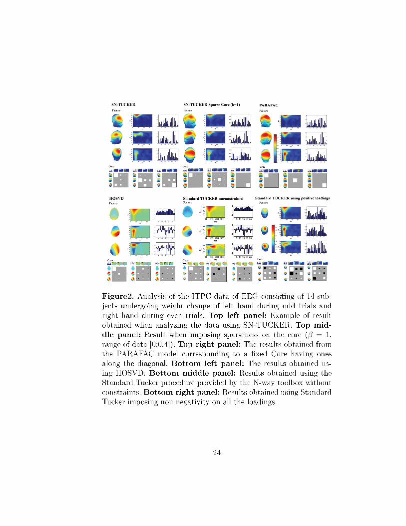
Figure2. Analysis of the ITPC data of EEG consisting of 14 sub-jects undergoing weight change of left hand during odd trials andright hand during even trials. Top left panel: Example of resultobtained when analyzing the data using SN-TUCKER. Top mid-

dle panel: Result when imposing sparseness on the core (β = 1,range of data [0;0.4]). Top right panel: The results obtained fromthe PARAFAC model corresponding to a �xed Core having onesalong the diagonal. Bottom left panel: The results obtained us-ing HOSVD. Bottom middle panel: Results obtained using theStandard Tucker procedure provided by the N-way toolbox withoutconstraints. Bottom right panel: Results obtained using StandardTucker imposing non-negativity on all the loadings.

24

Figure3. The result obtained analyzing the FIA data by a Tucker6-6-6 model. Top panel: SN-TUCKER based on LS with spar-sity on the Core and mixing modality, (β = 0.5 range of data [0;0.637]). Upper middle panel: Example of result obtained by aSN-TUCKER with no sparsity imposed. Lower middle panel: Ex-ample of decomposition obtained using the Standard Tucker proce-dure provided by the N-way toolbox imposing non-negativity on theloadings. The SN-TUCKER presently used LS minimization sincethis is the cost function the Standard Tucker also minimizes. Bot-tom panel: Result obtained from the corresponding 6 componentnon-negative PARAFAC decomposition.

25