Algorithms for Density, Potential Temperature ... for Density, Potential Temperature, ... Algorithms are presented for density, potential temperature, conservative temperature,

Algorithms for Density, Potential Temperature, Conservative Temperature, and theFreezing Temperature of Seawater

DAVID R. JACKETT AND TREVOR J. MCDOUGALL

CSIRO Marine and Atmospheric Research, Hobart, Tasmania, Australia

RAINER FEISTEL

Institut für Ostseeforschung, Warnemünde, Germany

DANIEL G. WRIGHT

Department of Fisheries and Oceans, Bedford Institute of Oceanography, Dartmouth, Nova Scotia, Canada

STEPHEN M. GRIFFIES

NOAA/Geophysical Fluid Dynamics Laboratory, Princeton, New Jersey

(Manuscript received 8 July 2005, in final form 30 March 2006)

ABSTRACT

Algorithms are presented for density, potential temperature, conservative temperature, and the freezingtemperature of seawater. The algorithms for potential temperature and density (in terms of potentialtemperature) are updates to routines recently published by McDougall et al., while the algorithms involvingconservative temperature and the freezing temperatures of seawater are new. The McDougall et al. algo-rithms were based on the thermodynamic potential of Feistel and Hagen; the algorithms in this study areall based on the “new extended Gibbs thermodynamic potential of seawater” of Feistel. The algorithm forthe computation of density in terms of salinity, pressure, and conservative temperature produces errors indensity and in the corresponding thermal expansion coefficient of the same order as errors for the densityequation using potential temperature, both being twice as accurate as the International Equation of Statewhen compared with Feistel’s new equation of state. An inverse function relating potential temperature toconservative temperature is also provided. The difference between practical salinity and absolute salinity isdiscussed, and it is shown that the present practice of essentially ignoring the difference between these twodifferent salinities is unlikely to cause significant errors in ocean models.

1. Introduction

McDougall et al. (2003, hereafter MJWF03) have re-cently fitted a 25-term rational function to seawaterdensity, when considered a function of salinity S, po-tential temperature �, and pressure p. The major moti-vation for the development of this equation of state wasthat ocean models have been cast in terms of potentialtemperature (rather than in situ temperature) as theirocean temperature variable, and an accurate and effi-

cient code for the computation of density in these termswas lacking. The 25-term equation was also motivatedby publication of the Feistel and Hagen (1995, hereaf-ter FH95) equation of state, which was based on aGibbs thermodynamic potential. This equation turnedout to be more accurate than, and addressed severalweaknesses in, the well-established International Equa-tion of State of Seawater (Fofonoff and Millard 1983).MJWF03 also presented a new algorithm for the com-putation of potential temperature that was thermody-namically consistent with the FH95 ocean density rou-tine. The algorithms they presented resulted in a codethat was substantially more efficient for computing den-sity and potential temperature than routines based onthe power series representation of the Gibbs potential,

Corresponding author address: Dr. David R. Jackett, CSIROMarine and Atmospheric Research, GPO Box 1538, Hobart, TAS7001, Australia.E-mail: [email protected]

DECEMBER 2006 J A C K E T T E T A L . 1709

© 2006 American Meteorological Society

JTECH1946

and achieved an accuracy for the important oceano-graphic variables of the same order as the accuracy ofthe Feistel and Hagen fits compared with the then mostrecently available ocean data.

More recently, Feistel (2003, hereafter F03) has up-dated the Gibbs potential by both the inclusion of newdata constraints and the addition of higher-order termsin its power series representation. Complete details ofall the improvements can be found in F03, but here wemention the recalibration of old seawater data for com-patibility with the 1995 international scientific pure wa-ter standard (IAPWS-95: Wagner and Pruß 2002) andinclusion of the triple point of water in the fit of theGibbs function. This has led to better sound speed es-timates at high pressures. Temperatures of maximumdensity are reproduced to the accuracy of the experi-mental data. The accuracy in fitting real ocean data hasalso been improved over that in FH95 by increasing byone the powers of temperature, salinity, and pressure inthe power series expression for the Gibbs potential.This leads to a potential function with 101 coefficients,resulting in more than a 20% increase in computationalcost over the 83-term power series of FH95.

Given these improvements in the Gibbs thermody-namic potential together with its increased computa-tional cost, a refit of the functions underlying the algo-rithms of MJWF03 seemed in order. Again, we havechosen rational functions as our fundamental fittingfunctions, owing to the rich and stable nature such func-tional representations provide. Although we could havechanged various terms in the 25-term rational functionapproximation to density �(S, �, p), we have chosen toretain the same terms for consistency with the corre-sponding routines in MJWF03 and for ease of imple-mentation in current ocean models. Although the num-ber of terms in the Gibbs potential has been increased,we find that the original form of our rational functionapproximation leads to fits with errors for key oceano-graphic variables of the same order as the correspond-ing errors of the Gibbs function fit of F03 to the under-lying thermodynamic data. We show that these errorsare approximately one-half of those arising from thespatial variability in the composition of seawater (Mil-lero 2000).

The thermodynamic variable whose advection anddiffusion most accurately represents the first law ofthermodynamics is potential enthalpy (McDougall2003), a variable easily computed from the Gibbs po-tential of either FH95 or F03, and it is convenient toform a new temperature variable, called conservativetemperature, by simply dividing potential enthalpy by afixed value of heat capacity. Complete details of thetheoretical justification for and the properties of this

conservative temperature variable can be found in Mc-Dougall (2003). Since ocean models treat their tem-perature variable as conservative, it is more appropri-ate to interpret ocean model temperature as conserva-tive temperature rather than the present practice,which is to interpret the model’s temperature as poten-tial temperature. To run ocean models with this tem-perature variable, an equation of state is needed that isa function of conservative temperature, salinity, andpressure, and we here present such an equation. Also,an algorithm is presented for the calculation of poten-tial temperature in terms of salinity and conservativetemperature so that, for example, sea surface tempera-ture can be calculated from an ocean model’s internalconservative temperature.

We also include a simple rational function for thefreezing point of seawater that is based on the new F03Gibbs thermodynamic potential in combination withthe new Gibbs function of ice (Feistel and Wagner2005, hererafter FW05). Throughout we use the sym-bols T, �, and � to represent the three temperaturevariables: in situ temperature, potential temperature,and conservative temperature—in degrees Celsius. Sa-linity, as usually measured and based on conductivitymeasurements, is denoted by S and absolute salinity,the mass of salt per mass of seawater (in grams perkilogram), is given the symbol SA. Pressure is denotedby p, density by �, and the reference pressure to whichpotential variables are referred is pr. All temperaturevariables are based on in situ temperature being mea-sured in °C on the 1990 International TemperatureScale (ITS-90: Preston-Thomas 1990), pressures are indecibars (1 dbar � 104 Pa), and salinity is expressed onthe Practical Salinity Scale 1978 (PSS-78: Lewis andPerkin 1981). All pressures are gauge pressures; that is,they are the absolute pressures less 10.1325 dbar.

In section 2 we update the algorithms found inMJWF03, while section 3 contains three algorithms as-sociated with conservative temperature: the forwardfunction, an equation of state, and an inverse function.Section 4 then deals with freezing temperature formu-las for in situ temperature, conservative temperature,and potential temperature. In section 5 we discuss thedifferences between absolute and practical salinity inocean models, and section 6 concludes the paper.

2. Updated algorithms for potential temperature�(S, T, p, pr) and the �(S, �, p) equation of state

Here we update the two algorithms appearing inMJWF03.

1710 J O U R N A L O F A T M O S P H E R I C A N D O C E A N I C T E C H N O L O G Y VOLUME 23

a. Potential temperature �(S, T, p, pr)

The routine for calculating the potential temperatureof seawater is identical to the corresponding algorithmin MJWF04, and the updated coefficients can be foundin section a of appendix A. We test the accuracy of thenew values of � by examining the root-mean-square(rms) and maximum absolute errors when 106 randomfluid parcels (S-T-p), drawn from the cube [0, 42 psu] �[�2°C, 40°C] � [0 dbar, 104 dbar], are referenced toanother 106 random pressures in the range [0 dbar, 104

dbar]. The potential temperatures against which wecompare the estimates of � are those obtained by iter-ating the standard Newton–Raphson technique fromthe in situ temperatures to their fixed points (see sec-tion a of appendix A). The accuracy of the recom-mended two iterations of the algorithm of the first sub-section of appendix A is 2.84 � 10�14 °C (maximumabsolute) and 3.50 � 10�15 °C (rms), respectively, effec-tively being machine precision. In terms of efficiency,the algorithm presented here for the computation of �is 3.5 times faster than the computation of � by iterationfrom T to the potential temperature fixed point.

The maximum difference between potential tem-perature (referenced to 0 dbar) determined from theentropy of FH95 (as in MJWF03) and the entropy ofF03 (as in this paper) for the ocean atlas data of Kol-termann et al. (2004; see also Gouretski and Kolter-mann 2004) is 3 mK, which is very similar to the differ-ence (2.5 mK) between � determined by the Fofonoffand Millard (1983) algorithm and that of MJWF03, asreported in that paper. Also, as discussed in MJWF03,an uncertainty in the thermal expansion coefficient of6 � 10�7 °C�1 leads to a maximum uncertainty in � � Tof 2 mK for a pressure difference of 5000 dbar. Weconclude that in the oceanographic range of variables,each of the three algorithms for � (i.e., Fofonoff andMillard 1983, MJWF03, and the present paper) differfrom each other by approximately the same amount.Nevertheless, the present approach is preferable for thecalculation of � since it uses the most accurate Gibbsfunction that is available to date and so is likely to bethe most accurate of the three methods.

b. The �(S, �, p) equation of state

Coefficients of the new �(S, �, p) equation of stateare given in section a of appendix A. To test the accu-racy of the new equation, uniformly distributed (S, T, p)points were taken from a “funnel” of data, very similarto but slightly larger than the funnel used in the corre-sponding fit in MJWF03. At the sea surface the mini-mum in situ temperature is taken to be 2°C below thein situ temperature at which seawater freezes at a pres-

sure of 500 dbar, and the maximum temperature is40°C, while salinity varies from 0 to 42. The minimumtemperature limit and the maximum salinity limit areindependent of pressure. The maximum temperaturelimit and the lower salinity limit are varied as linearfunctions of pressure so that the upper temperaturebound is 15°C, while the minimum salinity is 30 psu at5500 dbar. Below this pressure, temperature and salin-ity extremes are held constant all the way down to 8500dbar. While this funnel is used to set the range of valuesused in the fitting exercise, a slightly narrower and shal-lower funnel [from the freezing temperature (at 500dbar) up to 33°C at the sea surface and up to 12°C at5500–8000 dbar] is used to report the errors of the fit. Athree-dimensional view of this latter funnel is shown inFig. 1a while cross sections of the funnel are plotted assolid lines in Figs. 1b and 1c. The freezing temperatureplotted in Fig. 1c corresponds to a salinity value of 35psu. Also plotted in Figs. 1b and 1c are the extremes ofthe Koltermann et al. (2004) climatology (dashed lines)to indicate how real ocean data fits inside the narrowererror funnel.

Figure 2 shows the errors in (a) density �(S, �, p)(Fig. 2a), (b) the thermal expansion coefficient � ��1 ��/��|S, p, (c) the haline contraction coefficient � ��1 ��/�S|�, p, (d) sound speed from (cs)

�2 � ��/�p|S,�; all are plotted as functions of pressure. The solidlines in Fig. 2 show rms and maximum absolute differ-ences between these four variables and correspondingquantities computed directly from the in situ densityfunction of F03. Also shown in each panel as dashedlines are the rms and maximum absolute errors for datataken from the Koltermann et al. (2004) isopycnallyaveraged World Ocean climatology. The errors in �and should be compared with typical ocean atlas val-ues that are of order 1.5 � 10�4 K�1 and 7.5 � 10�4

(psu)�1, respectively. [While salinity measured on thePractical Salinity Scale does not strictly have a “unit,”there are many occasions where one needs to be spe-cific about the type of salinity that is used (e.g., whetherthe practical salinity scale is used or whether salinity isexpressed in kg kg�1 or g kg�1), and in these situationswe use the “psu” nomenclature.]

When compared with the corresponding figure ofMJWF03 (their Fig. 3), funnel errors in all the variableshere are 20%–160% larger than the corresponding er-rors in MJWF03. These errors could be lowered by theinclusion of more terms in the rational function or byexchanging terms in the 25-term rational function withterms involving other powers of S, �, and p. The latterpossibility was examined and resulted in only minorimprovements. However, the errors in Fig. 2 are al-ready of the same order as errors in the power series fit


of the Gibbs function in F03 to the underlying data, sowe decided that a change in functional form was notwarranted. For example, Table 9 of F03 indicates thatrms errors as large as 10�2 kg m�3 in density and 7.3 �10�7 K�1 in the thermal expansion coefficient are

present in the F03 fit. The rms errors in the data un-derlying the F03 fits are 3 � 10�2 kg m�3 for densityand 6.0 � 10�7 K�1 for the thermal expansion coeffi-cient. The errors in density shown in Fig. 2 are 2.4 �10�3 kg m�3 (rms) and 6.5 � 10�3 kg m�3 (max), and

FIG. 1. (a) A three-dimensional view and (b), (c) cross sections of the funnel over which theerror in the fit of our 25-term equation was evaluated. Dashed lines in (b) and (c) representextreme values of data taken from the Koltermann et al. (2004) climatology.

FIG. 2. (a) The rms and the maximum absolute errors in density �(S, �, p) as a function of pressure for data in the (S–T–p) funnelof Fig. 1 (solid lines). (b)–(d) These error measures for the thermal expansion coefficient, the haline contraction coefficient, and soundspeed, respectively. These figures are for the differences between our 25-term equation of state and the full F03 form of the equationof state. Dashed lines are for the climatological data of Koltermann et al. (2004).


those in the thermal expansion coefficient are 2.8 �10�7 K�1 (rms) and 9.8 � 10�7 K�1 (max), respectively.In terms of real ocean climatology the correspondingerrors are 1.9 � 10�3 kg m�3 (rms) and 4.9 � 10�3 kgm�3 (max), and 2.9 � 10�7 K�1 (rms) and 6.5 � 10�7

K�1 (max), respectively. All density and thermal ex-pansion coefficient rms errors of the �(S, �, p) fit arethus within the uncertainty of both available ocean dataand the F03 Gibbs potential fit to this ocean data. Forexample, the rms error in � in Fig. 2b of 2.8 � 10�7 K�1

is only 38% of the rms error in the � fit of F03 to theunderlying data. We therefore have no hesitation usingthe same rational function here as was used inMJWF03.

On the basis of this comparison of rms errors oneconcludes that our 25-term equation of state and F03yield equally accurate estimates of � and �. The maxi-mum absolute error in the haline contraction coeffi-cient in Fig. 2c is approximately 2 � 10�6 (psu)�1,which corresponds to a relative error of 0.25% of themean value of and is thus less important than thecorresponding errors in �. The rms errors of the soundspeed fit of F03 are at most 3.5 cm s�1 when fitting datathat has rms errors of 5 cm s�1. This is to be comparedwith typical rms errors of 26 cm s�1 in our equation(Fig. 2d) for both the funnel of data in Fig. 1 and theocean data of Koltermann et al. (2004). Given that thedensity computed from the Gibbs potential of F03 con-tains almost 3 times (73 terms) as many parameters asour 25-term equation of state, there will inevitably beoceanographic variables that F03 will represent moreaccurately than we can with our density equation. Wechose to accurately represent the thermal expansioncoefficient with our choice of penalty function and withour choice of terms, and this has been at the expense ofthe accuracy of sound speed. However, the maximumerrors in sound speed in Fig. 2d are still less than theextreme errors of several meters per second that existbetween the different sound speed formulas that ap-pear in F03. The comparison of 73 terms for the F03equation of state to 25 terms for the rational functionequation of state also clearly indicates the improvedefficiency in using the latter parameterization for oceandensity.

3. Algorithms associated with conservativetemperature �(S, �)

The first law of thermodynamics may be written as(Landau and Lifshitz 1959)

��dh

dt�

1�

dp

dt � � �� · FQ ��M,

where h is the specific enthalpy, defined by h � � (p0 p)/�, � is the internal energy, � is in situ density, pis the excess of the real pressure over the fixed atmo-spheric reference pressure, p0 � 0.101 325 MPa, d/dt ��/�t u · � is the material derivative following the in-stantaneous fluid velocity, FQ is the flux of heat by allmanner of molecular fluxes and by radiation, and � �M

is the rate of dissipation of kinetic energy (in units of Wm�3) into thermal energy. The effect of the dissipationof kinetic energy in these equations is very small and isalways ignored in the oceanic context. McDougall(2003) has shown that the left-hand side can be approxi-mated by �dh0/dt, where h0 is the potential enthalpyreferenced to 0 dbar, with additional terms that are zeroat the sea surface and are not larger anywhere than thedissipation of mechanical energy. Hence, the first law ofthermodynamics in the ocean can be expressed as �dh0/dt � �� · FQ. It is this form of the first law that canthen be Reynolds averaged to obtain an equation inwhich the turbulent fluxes of potential enthalpy aremuch larger than the molecular fluxes of heat so thatpotential enthalpy is the oceanic variable that encapsu-lates what we mean by the “heat content” of seawater.That is, potential enthalpy is the variable whose advec-tion and turbulent diffusion throughout the ocean canbe accurately compared with the boundary fluxes ofheat. The error involved in making this statement is nolarger than those associated with ignoring the dissipa-tion of mechanical energy and is two orders of magni-tude less than the error that is incurred in the presentoceanic practice of treating potential temperature as aconservative variable.

This section of the paper contains three algorithmsthat are required by an ocean model so that its tem-perature conservation equation can be an accurate em-bodiment of the first law of thermodynamics.

a. The forward function �(S, �)

Conservative temperature is defined to be propor-tional to potential enthalpy. Full details on the precisedefinition of conservative temperature � as a functionof salinity S and potential temperature � (referred to 0dbar) can be found in section a of appendix B.

In Fig. 3, we show the differences � � � betweenpotential temperature and conservative temperature onthe S–� diagram. This temperature difference has beendeliberately designed to be small for much of theoceanographically relevant regions of S–� space. Theseregions are shaded gray based on real ocean data takenfrom the Koltermann et al. (2004) climatology. The dif-ference between the present definition of �, which isbased on the Gibbs function of F03 and that of McDou-gall (2003) based on the FH95 Gibbs function, is shown


in Fig. 4. The most obvious feature of Fig. 4 is the lineartrend in S, but this is thermodynamically irrelevant be-cause enthalpy is unknown and unknowable up to alinear function of salinity; that is, as explained by FH95,

no thermodynamic measurement can distinguish be-tween two versions of enthalpy that differ by a linearfunction of salinity. The trend has been caused by shift-ing the reference point used for pure water from T �

FIG. 3. Differences � � �F03 between potential temperature and conservative temperaturebased on the F03 Gibbs potential over the S–�F03 plane. Also plotted in gray are real oceandata points taken from the Koltermann et al. (2004) climatology.

FIG. 4. Differences �FH95 � �F03 between conservative temperature based on the FH95 andthe F03 Gibbs potential over the S–�F03 plane. The gray points again correspond to real oceandata points taken from the Koltermann et al. (2004) climatology.


0°C, p � 0 dbar in FH95 to the triple point in F03, butwith zero offset for the standard ocean, T � 0°C andS � 35 psu. When this linear trend in S is subtracted,one finds that the maximum difference between the twodefinitions of � is only 0.003°C, which is approximatelytwo orders of magnitude less than the differences, � ��, contained in Fig. 3. This maximum difference of0.003°C in the two definitions of � based on the Gibbsfunctions of FH95 and F03 is primarily due to the dif-ferent heat capacity data that was used in those papersto fit the respective Gibbs functions. As explained inF03, the earlier Gibbs function of FH95 [as well asFofonoff and Millard (1983) heat capacity] was basedon quite old heat capacity data of freshwater that werepublished between 1902 and 1927.

Table 9 of F03 shows that the heat capacity datapublished in the 1970s, which had an rms error of 0.5 J(kg K)�1, is reproduced by the F03 Gibbs function to anrms accuracy of 0.54 J (kg K)�1. To obtain an estimateof the corresponding error in �, we assume that theremaining error in the heat capacity of F03 is of orderone-half of this value. Integrating a heat capacity errorof 0.25 J (kg K)�1 over a temperature range of 15°C anddividing by a nominal heat capacity, we obtain 0.001°Cas an estimate of the rms error in �. This is almost thesame as the estimate from McDougall (2003) of theaccuracy with which � is a conservative variable thatrepresents the heat content of seawater. We concludethat the conservative temperature of Eq. (B1) (andTable B1) is more accurate than that based on FH95and that any remaining uncertainty in � is at the levelof 1 mK, being approximately equally due to the re-maining uncertainty in the Gibbs function of seawaterand to the nonconservation of potential enthalpy in theocean. The practice to date in oceanography essentiallyhas heat content being proportional to � rather than to�, even though we know that the rms and maximumvalues of |� � �| in the World Ocean are 0.018° and1.4°C, respectively (from McDougall 2003). This doesnot appear to be justifiable: we recommend adoptingthe algorithm (B1) and Table B1 as the definition of �.

When an ocean model is run with conservative tem-perature as its temperature variable, the model needsto be initialized with �, and one wonders whether it issufficiently accurate to use an existing ocean atlas thatcontains the averaged values of S and �, namely, S and�, and simply calculate the initial � field as �(S, �). Thisis not quite the same as the averaged value of conser-vative temperature, �, because the functional relation-ship between these variables is nonlinear. Expanding�(S, �) as a Taylor series about the mean values S and� and averaging, we find that

� ��S, �� 12

��2 �S��S� 12

�SSS�2

where the second-order partial derivatives are evalu-ated at (S, �) . As explained after Eq. (B5) of McDou-gall (2003), the term proportional to ��S� is larger thanthe other two so that � � �(S, �) �S��S� � 1.4 �10�3 ��S� with S� measured on the practical salinityscale. With perfectly correlated perturbations of mag-nitude 3°C and 1 psu, the estimated difference � ��(S, �) 4 mK, which is likely small enough to beignored. These small nonlinear differences in tempera-ture arise because potential temperature is not a con-servative variable, so � should not have been averagedduring the process of forming the atlas. The thermody-namic variable that is conserved on mixing at a certainpressure is enthalpy and, when mixing occurs at depthin the ocean, not even � is 100% conserved. For ex-ample, Eq. (C8) of McDougall (2003) shows that whenmixing occurs at a pressure of 600 dbar between watermasses that differ in temperature by 2°C, the resultingvalue of � is different from � by about 10�5 °C. Weconclude that the error involved in averaging � to forma local averaged value is likely to be no more than a fewmillikelvin, while the error involved with averaging � isestimated to be no more than 10�5 °C.


With the temperature in an ocean model being re-garded as conservative temperature, an equation ofstate �(S, �, p) is needed, that is, an expression for insitu density written in terms of this new temperaturevariable. The complete details of the form of this equa-tion, its coefficients, and check values can be found inthe second subsection of appendix B.

As in section 2b, the funnel used for the evaluation ofthe rational function is slightly smaller than the funnelused to obtain the fitted rational function. The differ-ence between our 25-term equation of state and the F03“truth” is illustrated in Fig. 5. Both rms and maximumabsolute errors are shown as functions of pressure fordata in the (S–T–p) funnel shown in Fig. 1. Also shownare the corresponding rms and extreme errors for thereal ocean data of Koltermann et al. (2004). Figure 5ashows that the maximum error in density is less than0.006 kg m�3, while the rms error is less than half thisvalue. The other panels of Figures 5 show the errors inthe thermal expansion coefficient �, the haline contrac-tion coefficient , and the sound speed cs that resultfrom the errors in our 25-term equation of state whencompared with the corresponding coefficients obtained


using the full Gibbs function of F03. The first deriva-tive coefficients for conservative temperature are de-fined by

� � ��1��|S,p, � ��1��S|�,p,�cs�

�2 � ��p|S,�. �1�

Note that � and defined here are slightly differentfrom the corresponding coefficients defined inMJWF03 and section 2b above because in one casedifferences are taken with respect to (or at constant) �and in the other case with respect to (or at constant) �.In both cases, however, the expressions for the soundspeed are the same (since ��/�p|S,� � ��/�p|S,�) and thebuoyancy frequency N can be expressed by the obviousexpressions. That is, g�1N2 � � �z � Sz using the �and from section 2b, while g�1N2 � � �z � Sz whenusing the � and from (1). Similarly, the horizontaldensity gradient is given both by

��1�H� � ��1��p�|S,��Hp � �HS � ��H�,

using the � and from section 2b, and by

��1�H� � ��1��p�|S,��Hp � �HS � ��H�,

when using the � and from Eq. (1).Figure 5b shows that the maximum error in the ther-

mal expansion coefficient is less than 9.9 � 10�7 °C�1,while the rms value is, apart from the surface mixedlayer, less than 3.5 � 10�7 °C�1. As explained inMJWF03, the key accuracy measure for physical ocean-ography is this maximum error in the thermal expan-

sion coefficient, which here is equivalent to a relativeerror in the thermal expansion coefficient of less than0.7%. The maximum error in the saline contraction co-efficient of 1.6 � 10�6, which corresponds to a relativeerror of 0.2% of the mean value of , is thus much lessimportant than the corresponding error in �. As in sec-tion 2b, we have not paid much attention to the error insound speed but we note that the errors in our Fig. 5dare again significantly less than the extreme differencesof several meters per second reported in F03 betweenthe various sound speed formulas. In Figs. 5a–d theaverage values of the rms errors and the maximum ab-solute errors for the real ocean climatological data ofKoltermann et al. (2004) (dashed lines) are consistentlyless than the corresponding quantities for the largerocean funnel data. Note, however, that there are sub-stantial pressure intervals over which the rms errors forthe ocean climatological data (legitimately) exceed therms errors for the funnel data of Fig. 1.

The rms error in � of 3.5 � 10�7 °C�1, shown in Fig.5b, is only 48% of the rms error in the � derived fromthe Gibbs function fit of F03 to the underlying data. Wehave also calculated the differences between the ther-mal expansion coefficient based on the FH95 Gibbsfunction and the F03 Gibbs function over the same fun-nel for both potential and conservative temperature,and find that these differences are about 3 times aslarge as our maximum error in Fig. 2b and Fig. 5b. Thisresult can also be confirmed from Fig. 21b of F03. Weconclude that our 25-term equations of state are as ac-curate as the data from which F03 was derived and that

FIG. 5. As in Fig. 2 but for �(S, �, p).


there is a marginal increase in accuracy with the updatefrom FH95 to F03.

As in the case of the equation of state in terms of S,�, and p of section 2b, the equation of state in terms ofS, �, and p with 25 terms is a substantially more effi-cient parameterization of ocean density than is theequation of state of F03 with 73 terms. Indeed the ra-tional function equations of state can be coded withonly 26 multiplications, one square root, and one divi-sion compared with the F03 equation of state that canbe coded with 73 multiplications, one square root, andone division, a clear savings in time.

We need to emphasize that the pressure argument inall of these equations of state (including those of FH95,MJWF03, F03, and the present paper) is the gauge pres-sure in decibars, defined as the absolute pressure indecibars less 10.1325 dbar (see FH95 and F03). Thepressure variable in ocean models is sometimes abso-lute pressure, and the failure to take account of thedifferent definitions of pressure would lead to an errorin the thermal expansion coefficient of approximately

� � �10.1325db��p�|S,� 2.7 � 10�7 K�1

[see Fig. 9b of McDougall (1987) for the estimate of(��/�p)|S,�], which is similar to the rms error in our fitof the thermal expansion coefficient to that of F03.Since this error is virtually constant over the wholeocean, it is clearly more serious than the fitting rmserror of this magnitude that is as often positive as nega-tive. Hence, one must be careful to evaluate the equa-tion of state with gauge pressure rather than with ab-solute pressure.

c. The �(S, �) inverse function

During the running of an ocean model the interiortemperature is best interpreted as conservative tem-perature �, and the appropriate form of the equation ofstate is the one expressed in terms of �, such as de-scribed in section 3b above. If an ocean model is beingrun with fixed sea surface temperature and fixed seasurface salinity, then the sea surface values of � canalso be fixed. However, when the ocean is allowed tointeract with the atmosphere, the real SST will beneeded as an input to the “bulk formulae” for the air–sea heat flux. An inverse algorithm � � �(S, �) is thusrequired for converting salinity S and conservative tem-perature � into potential temperature �. Section c ofappendix B contains the full details of this inverse func-tion.

The maximum absolute and rms errors for the com-putation of potential temperature for 104 uniformlygenerated data points over the S � � plane 0 � S � 42,

� 2°C � � � 40°C are, respectively, 6.02 � 10�14 °Cand 3.78 � 10�15 °C, justifying the effort in finding agood starting value of � in (B7) and just one iteration of(B8). These were obtained by first computing conser-vative temperature using the forward function in sec-tion a of appendix B and then inverting using the tech-nology of section c of appendix B. The errors reportedabove are effectively machine precision, and appear aswhite noise showing no structure when plotted on theS � � plane. As with the algorithm for potential tem-perature in section 2a, the algorithm for computing po-tential temperature from conservative temperaturehere runs 3.5 times as fast as iterating the full Newton–Raphson solution of �(S, �) � � to the fixed-pointsolution with � as the initial estimate of potential tem-perature.

As mentioned above, for an ocean model interactingwith the atmosphere, the inverse algorithm for�(S, �) will generally need to be used at each modeltime step to determine the SST at the surface grid levelin the ocean. Since this needs to be done only at the onehorizontal level and since the computer time involvedin evaluating � is only a couple of times the cost ofperforming an equation of state evaluation, the com-puting time required to evaluate SST will not be a sig-nificant issue.

4. The freezing temperatures Tf(S, p), �f(S, p), and�f(S, p)

The commonly used algorithm for the calculation offreezing point temperatures is that of Millero and Le-ung (1976), a four-term polynomial that has beenadopted by the United Nations Educational, Scientificand Cultural Organization through Fofonoff and Mil-lard (1983) for the pressure range up to 500 dbar (Mil-lero 1978). The estimated error of this routine whencompared to the data of Doherty and Kester (1974) is 3mK at atmospheric pressure. Its high pressure part isderived by thermodynamic rules (Clausius–Clapeyronequation) and deviates by about the same amount fromthe data of Fujino et al. (1974) down to a pressure of500 dbar. Both FH95 and F03 have fitted these samedata at one atmosphere, as well as additional more re-cently available data and standards of freshwater andice for higher pressures, in F03’s case with an rms errorof 1.5 mK. Simplified polynomial expressions for thefreezing point based on FH95 were published by Feisteland Hagen (1998). The freezing points given in F03 arecomputed using a slightly modified version of theformer Feistel and Hagen (1998) Gibbs potential of ice,which is to be replaced now by the new and more ac-curate one of FW05. Here we fit the freezing tempera-tures of the most recent ice Gibbs function of FW05 to


within the same error tolerances as the F03 fit to data,using 11-term rational functions (with only nine un-known parameters). Three fits are made, one for eachof the temperature variables—in situ temperature T,potential temperature �, and conservative temperature�. Complete details can be found in appendix C.

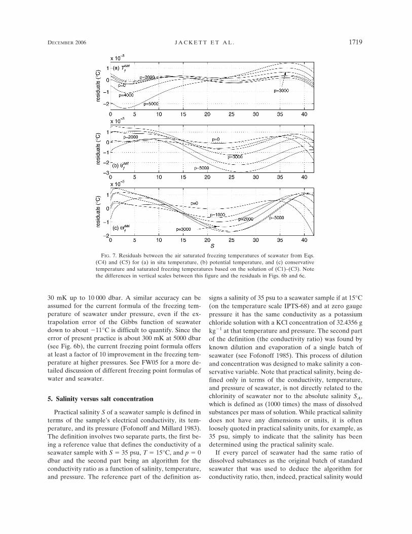
Figure 6a shows the (in situ) freezing temperature ofair-saturated seawater as a function of salinity and pres-sure, showing the strong linear dependence on bothsalinity and pressure. The differences between the for-mula of Millero and Leung (1976) and the freezing tem-peratures from the full Newton–Raphson iterative so-lution to (C1)–(C3) [and using (C5)] are displayed inFigs. 6b and 6c. It is seen that at a pressure of 1000 dbarthe error in the Millero and Leung (1976) formula isabout 12.5 mK near S � 35 psu. The error increases athigher pressures so that at 3000 dbar the error is 130mK. Corresponding residuals, again relative to the so-lution of (C1)–(C3) using (C5), for the three freezingtemperatures defined by (C5) and (C4) are shown inFig. 7. All residual plots are for saturated freezing tem-peratures and are plotted as functions of salinity for arange of pressures. Figure 7 clearly shows that the maxi-mum errors in our fit at p � 2000 dbar are of order 1mK for each of the three temperature variables,

whereas the error in the Millero and Leung (1976) poly-nomial is of order 50 mK at this pressure.

Even in cases of negative lapse rates, that is, when awater parcel cools down by compression (McDougalland Feistel 2003), the freezing point lowering by pres-sure (Clausius–Clapeyron equation) significantly ex-ceeds the adiabatic cooling (Feistel and Wagner 2005).Thus, independent of the salinity of a given liquid waterparcel, freezing due to pressure change can only occurduring expansion (rising) and never during compres-sion (sinking). In other words, freezing of a parcel isimpossible at any depth as long as its potential tem-perature is higher than its surface (in situ) freezingpoint.

The FW05 freezing point for pure air-free water atone atmosphere is accurate with only 2 �K error, and itreproduces the Doherty and Kester (1974) freezingpoints of seawater at atmospheric pressure within theirexperimental scatter of 2 mK. Due to the significantlymore accurate compressibility of ice in the FW05 for-mulation in comparison to various values discussed inthe literature (Dorsey 1968; Yen 1981) and the onesused by Millero (1978) or in FH95 and F03, the high-pressure freezing point measurements of Hendersonand Speedy (1987) for pure water are met now within

FIG. 6. (a) In situ freezing temperature of seawater and (b), (c) differences between thefreezing temperatures of Millero and Leung (1976) and the in situ freezing temperature ofseawater, each saturated with air from the solution of (C1)–(C3) and (C5a). Panel (c) is simplyan expanded view of (b).


30 mK up to 10 000 dbar. A similar accuracy can beassumed for the current formula of the freezing tem-perature of seawater under pressure, even if the ex-trapolation error of the Gibbs function of seawaterdown to about �11°C is difficult to quantify. Since theerror of present practice is about 300 mK at 5000 dbar(see Fig. 6b), the current freezing point formula offersat least a factor of 10 improvement in the freezing tem-perature at higher pressures. See FW05 for a more de-tailed discussion of different freezing point formulas ofwater and seawater.

5. Salinity versus salt concentration

Practical salinity S of a seawater sample is defined interms of the sample’s electrical conductivity, its tem-perature, and its pressure (Fofonoff and Millard 1983).The definition involves two separate parts, the first be-ing a reference value that defines the conductivity of aseawater sample with S � 35 psu, T � 15°C, and p � 0dbar and the second part being an algorithm for theconductivity ratio as a function of salinity, temperature,and pressure. The reference part of the definition as-

signs a salinity of 35 psu to a seawater sample if at 15°C(on the temperature scale IPTS-68) and at zero gaugepressure it has the same conductivity as a potassiumchloride solution with a KCl concentration of 32.4356 gkg�1 at that temperature and pressure. The second partof the definition (the conductivity ratio) was found byknown dilution and evaporation of a single batch ofseawater (see Fofonoff 1985). This process of dilutionand concentration was designed to make salinity a con-servative variable. Note that practical salinity, being de-fined only in terms of the conductivity, temperature,and pressure of seawater, is not directly related to thechlorinity of seawater nor to the absolute salinity SA,which is defined as (1000 times) the mass of dissolvedsubstances per mass of solution. While practical salinitydoes not have any dimensions or units, it is oftenloosely quoted in practical salinity units, for example, as35 psu, simply to indicate that the salinity has beendetermined using the practical salinity scale.

If every parcel of seawater had the same ratio ofdissolved substances as the original batch of standardseawater that was used to deduce the algorithm forconductivity ratio, then, indeed, practical salinity would

FIG. 7. Residuals between the air saturated freezing temperatures of seawater from Eqs.(C4) and (C5) for (a) in situ temperature, (b) potential temperature, and (c) conservativetemperature and saturated freezing temperatures based on the solution of (C1)–(C3). Notethe differences in vertical scales between this figure and the residuals in Figs. 6b and 6c.


be a conservative variable (i.e., S would be exactly pro-portional to the conservative variable SA), at least tothe accuracy with which the conductivity ratio measure-ments were made and the algorithm was fitted to thatdata. Even in the major ocean basins there are smallvariations of the ratio of dissolved substances in seawa-ter that affect density, conductivity, and absolute salin-ity in ways that are not taken into account by the defi-nition of practical salinity or by the Gibbs function ofseawater of F03. There are two related issues here; thefirst is the relationship of the measured conductivity(and therefore, by definition, practical salinity S) to ab-solute salinity, and the second is the connection to den-sity. The first issue is the subject of this section of thepaper.

To relate practical salinity S to absolute salinity SA

one needs to know the concentrations of all the con-stituents of seawater, and Millero and Leung (1976)estimated the relationship [where SA is in parts perthousand [ppt (or °/°°)] as

SA � 1.004 880 S. �2a�

This relationship was updated by F03 using Millero’s(1982) mass fractions of seawater constituents to

SA � 1.004 867 S. �2b�

[Note that we have corrected an obvious typographicalerror in Eq. (53) of F03; Feistel 2004.] However, thecalculation is sensitive to the ratio of ingredients thatare taken to compose seawater, and taking the list ofconstituents from Culkin (1965) leads to the alternativelinear relationship (Fofonoff 1992)

SA � 1.0040 S. �2c�

It is clearly not straightforward to relate absolute sa-linity SA to practical salinity S. Nevertheless, settingaside marginal seas, we take as a working hypothesisthat in the major ocean basins SA lies in the range givenby Eqs. (2a)–(2c); namely,

SA � �1.0045 � 0.0005� S. �2d�

Note that the freshwater concentration (FW) in seawa-ter is given by

FW � �1 � 0.001SA� �1 � 1.0045 � 10�3 S�.

�3�

The approximately 0.45 � 0.05 % difference betweenS and SA is not trivial; for example, a seawater parcelwith S � 35 psu has an absolute salinity SA of between35.140 and 35.175 ppt, a difference of approximately

0.16 ppt, which is between 50 and 100 times as large asthe accuracy with which we can determine salinity atsea. Ocean models interact with the atmosphere(through the evaporation and precipitation E � P offreshwater) as though the variable that is labeled salin-ity in the model is actually absolute salt concentrationSA (in ppt), and yet in other parts of ocean model codethe salinity is regarded as practical salinity (for examplein the equation of state). We ask here what is the cor-rect interpretation of the model’s salinity and alsowhether ocean models suffer any significant error dueto the different definitions of salinity.

Interpreting the model’s salinity as absolute salinitySA, evaporation and precipitation cause the tendency ofabsolute salinity (SA)t of the uppermost model box tobe proportional to the product SA (E � P). With theinterpretation of the model’s salinity as practical salin-ity S, the salinity tendency of the uppermost modellayer includes a contribution St � S (E � P) associatedwith the surface freshwater fluxes. Given our presentknowledge of seawater thermodynamics, it seems rea-sonable to assume that S is exactly proportional to SA,and in this case there is actually no error involved withthe present implementation of the surface freshwaterboundary condition if the model salinity is interpretedas S. That is, existing ocean models have E � P affect-ing S in exactly the correct manner, just as E � P wouldaffect SA if the model variable were interpreted as SA.The combination of (i) the lack of any separate flux ofsalt across the sea surface and (ii) the exact proportion-ality of S and SA enables the present surface boundarycondition to be exact. [As a counterexample, if therehappened to be a surface input of buckets of crystallinesea salt (in units of kilograms of salt per square meter),then this would be accurately accounted for in the SA

budget but not in the budget of practical salinity S.] Asfar as the rest of the model domain is concerned, thesalt conservation equation is equally true whether writ-ten in terms of SA or in terms of S, and with the equa-tion of state in today’s models being expressed as afunction of S, models are calculating density consis-tently.

In summary, it seems that, despite the fact that prac-tical salinity is not the same as absolute salinity, presentmodels do not incur errors when they relax their salin-ity to values of S when they interact with an atmospherethrough freshwater fluxes, when they advect and dif-fuse S, and when they evaluate the equation of state interms of practical salinity. Hence, it would seem thatthe interpretation of the model variable as practicalsalinity S is error free. The only slight complication isthat, when one wants to calculate the freshwater frac-


tion exactly, one needs to use the expression from (3),namely, FW (1 � 1.0045 � 10�3 S) and, strictlyspeaking, this should be used when calculating the me-ridional flux of freshwater for an ocean basin (e.g., theIndian Ocean or the South Pacific Ocean). Also, mod-ern ice models allow for ice that is not completely freshbut rather contains small amounts of salt, and thisslightly salty ice is exchanged with the ocean as waterfreezes and melts. It is assumed that the salinity of thisice can be interpreted as being measured on the prac-tical salinity scale rather than as absolute salinity, and inthis case, no error would be incurred in the interactionbetween ice and ocean.

An alternative modeling approach is to interpret themodel’s salinity as absolute salinity. To be able to in-terpret the model’s salinity as SA, three changes topresent modeling practice are required: first in the re-storing boundary condition (if used) where the resto-ration would need to be to fixed values of SA ratherthan of S, second in the equation of state which wouldneed to be written in the functional form �(SA, �, p)rather than as �(S, �, p), and third in the initial condi-tions for a model run where it is imperative that theinitial salinity field is SA rather than S. If this third pointwere not done, the total amount of salt in the oceanwould be in error by 0.45% for the whole model run, asthere is no salt flux into or out of the ocean unless arestoring boundary condition is employed. With thesethree changes, the freshwater content and freshwaterfluxes could then be evaluated exactly using FW �(1 � 0.001 SA), and the salinity of sea ice would also beinterpreted as being absolute salinity. These threechanges to modeling practice could readily be imple-mented if it was deemed important to be able to deter-mine the freshwater content directly in terms of themodel’s salinity variable but, at this point, it is not ob-vious that this is a significant issue.

6. Discussion

One of the aims of the present work is to update thealgorithms of McDougall et al. (2003) for the compu-tation of potential temperature and density of seawater.The new algorithms are based on the latest seawaterGibbs potential of Feistel (2003), which is an improve-ment over the earlier Gibbs potential of Feistel andHagen (1995) in both computational accuracy and inthe extent of the oceanic data utilized in the formula-tion of the Gibbs potential. We have also determined afunction for computing the freezing temperature of sea-water that is consistent with the latest Gibbs potentials

of seawater (Feistel 2003) and ice (Feistel and Wagner2005).

Various algorithms involving the new conservativetemperature variable of McDougall (2003) have alsobeen presented. These include the definition of conser-vative temperature from the potential enthalpy func-tion of Feistel (2003), together with a function for thedensity of seawater written in terms of conservativetemperature and an inverse function for computing po-tential temperature from salinity and conservative tem-perature. All conservative temperature routines arebased on the Feistel (2003) Gibbs potential.

Although the rms and maximum absolute differencesrelative to F03 for the two density equations reportedhere are larger than the corresponding differences rela-tive to FH95 for the density equation of McDougall etal. (2003), the rms differences for density and the ther-mal expansion coefficient are still below the corre-sponding rms errors present in both the Feistel (2003)fits and in the oceanic data underlying these fits. Fol-lowing MJWF03, we have concentrated on the relativeerrors in the thermal expansion coefficient and in thesaline contraction coefficient, as these are the only er-rors in the equation of state that have dynamical con-sequences in ocean models. As explained in MJWF03,any error in density that is a function only of pressureand is independent of salinity and conservative tem-perature does not affect ocean dynamics either throughthe computation of horizontal pressure gradients or inthe calculation of vertical static stability.

From Figs. 5a and 5b of MJWF03 we see that themaximum errors in density and thermal expansion ofthe International Equation of State over the volume ofour funnel are �0.012 kg m�3 and �2.5 � 10�6 K�1,while the present Figs. 2 and 5 show that the corre-sponding maximum errors are about �0.006 kg m�3

and �0.95 � 10�6 K�1. These measures of accuracy areonly relevant if the F03 Gibbs function is equally asaccurate. This question can be addressed by the com-parison of F03 densities with the measurements ofBradshaw and Schleicher (1970) and also by consider-ing how well the F03 Gibbs function reproduces themeasurements of the temperature of maximum density(TMD). Bradshaw and Schleicher measured differ-ences in specific volume as temperature varied at fixedpressure and salinity for samples in the salinity rangebetween 30 and 40 psu. Figure 24a of F03 shows that theBradshaw and Schleicher (1970) data is fitted by theF03 Gibbs function with a maximum density error of nomore than �0.004 kg m�3 in the range of temperaturesand pressures in our funnel. This amounts to an upperbound on the thermal expansion coefficient of F03 for


oceanographic data from our funnel of no more than�0.4 � 10�6 K�1 in the salinity range 30 � S � 40 psu.

Measurements of the TMD data of Caldwell (1978)provide a rather direct estimate of the accuracy of thethermal expansion coefficient for very cold and freshseawater. From Table 9 of F03, we see that the rmserror in the thermal expansion coefficient derived fromF03 is �0.73 � 10�6 K�1 with respect to the TMD dataof Caldwell (1978). This fitting error is also approxi-mately the experimental error in the TMD data itself.

Taking this and the agreement between F03 and theBradshaw and Schleicher (1970) specific volume datameans that it is very likely that the maximum densityerror in the range of temperatures and pressures in ourfunnel in Figs. 2 and 5 is no more than �0.006 kg m�3,while the maximum error in our thermal expansion co-efficients is �0.95 � 10�6 K�1. In the salinity range30 � S � 40 psu, typical of values in the ocean atlas, itseems that the absolute accuracy of our algorithms fordensity and thermal expansion for water of standardcomposition may be �0.005 kg m�3 and �0.6 � 10�6

K�1, respectively.Another uncertainty remaining in the equation of

state and in the determination of salinity from oceanicobservations is due to spatial variations in the relativeconcentrations of alkalinity, total carbon dioxide, andsilica. Brewer and Bradshaw (1975) and, more recently,Millero (2000) have shown that for given values of con-ductivity, temperature, and pressure the range of un-certainty of density is up to 0.020 kg m�3 between themajor ocean basins; we will characterize this uncer-tainty as �0.010 kg m�3. Since the maximum densityerror of the International Equation of State (Fofonoffand Millard 1983) is about �0.012 kg m�3 and the maxi-mum error in the present equation of state is �0.005 kgm�3, we conclude that the uncertainty in oceanic com-position is as serious as the errors in the InternationalEquation of State of standard seawater and is a largerissue (by a factor of 2) than any remaining uncertaintyin either F03 or the fit to F03 contained in the presentwork. One could imagine mounting a concerted cam-paign to reduce these errors by, for example, obtainingmore accurate measurements of the temperature ofmaximum density so as to improve the accuracy of thethermal expansion coefficient. However, this activitywould only be worthwhile if one could simultaneouslyaddress the issues raised by Millero (2000) to accountfor the variation of the composition of seawater.

The rms errors in our freezing temperature equationare of the same order as the rms errors in the freezingtemperatures in F03, and the present freezing tempera-ture equations are much more accurate than the equa-tion in use today.

Oceanography traditionally uses salinity evaluatedon the practical salinity scale S, but the freshwater con-centration of seawater is not (1 � 0.001 S) but, rather, isgiven in terms of the absolute salt concentration SA by(1 � 0.001 SA). Even though S and SA differ by about0.45%, because the air–sea interaction involves onlyfluxes of freshwater and not of salt, we have shown thatignoring the distinction between S and SA does notcause errors of this magnitude.

Of the remaining issues with the equation of stateand the thermodynamics of seawater, the largest thatneeds to be addressed by ocean models is the changingof an ocean model’s temperature variable from poten-tial temperature � to conservative temperature � sincea typical maximum error in � � � of 0.25°C causes adensity difference of 0.05 kg m�3. This is a factor of atleast 5 larger than the density errors that we believeremain due to the uncertainty in the equation of state.(Actually, � � � is as large as 1.4°C in restricted areasof the World Ocean.)

Another temperature-like variable can be defined asproportional to specific entropy [see Fig. 5 of McDou-gall (2003)], but from the second law of thermodynam-ics, we know that entropy is not a conservative variablesince there is a net production of entropy wheneverdiffusion and mixing occur. Hence, it is clearly not ap-propriate as an approximation to “heat content” in theocean. However, one finds that the rms and maximumabsolute differences between this “entropic tempera-ture” and � are 0.33° and 0.5°C, respectively, so forextreme water masses (particularly for warm freshwa-ter) entropy is actually closer to being a conservativevariable than is potential temperature. An alternativemeasure of the errors associated with these variables isthe range of temperature differences outside ofwhich 1% of the data reside. McDougall (2003) reportsthat 1% of the � � � values at the sea surface of theWorld Ocean lie outside an error range of 0.25°C(�0.15°C � � � � � 0.10°C), which provides a conve-nient measure of the error associated with ocean mod-els that treat � as conservative. The correspondinganalysis for entropic temperature shows that 1% of thesurface data lie outside an error range of 0.53°C (0.5%have a temperature difference less than �0.21°C and0.5% exceed a difference of 0.32°C ). This error mea-sure suggests that � is only about a factor of 2 moreconservative than entropy. It seems clear that � is alsonot an appropriate approximation to the conservativeheat content of seawater. It is probably time to abandonthis practice.

Software for the algorithms described in this papercan be obtained on the Internet (available online atwww.marine.csiro.au/�jackett/eos).


Acknowledgments. This work is a contribution to theCSIRO Climate Change Research Program.

APPENDIX A

Algorithms Based on Potential Temperature

a. Updated coefficients for potential temperature�(S, T, p, pr)

The potential temperature of a fluid parcel (S, T, p)when referenced to a pressure pr is defined as that tem-perature � for which

��S, �, pr� � ��S, T, p�, �A1�

where specific entropy � is given by the first derivativeof the Gibbs potential g(S, T, p) with respect to tem-perature, �(S, T, p) � ��g(S, T, p)/�T. The solution of(A1) is achieved with the modified Newton–Raphsontechnique described in MJWF03. The only coefficientsrequiring updating from MJWF03 are the coefficientsfor the initial rational function approximation for � andthe constant first guess for �T at constant S and p � pr.Otherwise, all details are exactly as in MJWF03. TableA1 contains the new rational function coefficients while13.6 J kg�1 K�1 is the (constant) first estimate of �T.We recommend two iterations of this technique thatyield rms and maximum absolute errors of 3.50 �10�15 °C and 2.84 � 10�14 °C, respectively, when com-pared to the fixed-point Newton–Raphson solutions of(A1). A check value for the new potential temperaturealgorithm is

��35, 20, 4000, 0� � 19.2110837430117 C.

Note that this calculation of potential temperature re-produces the potential temperatures of Table 19 of F03.

b. Updated coefficients for the density equation �(S,�, p)

The 25-term equation of state for in situ density (inkg m�3), when expressed as a function of salinity S(PSS-78), potential temperature � (in °C), and pressurep (in dbar), is taken to have the same form as the cor-responding equation in MJWF03; namely,

��S, �, p� � Pn�S, �, p��Pd�S, �, p�, �A2�

where the polynomials Pn(S, �, p) and Pd(S, �, p) aredefined as in Table A2. Here � is potential temperaturereferenced to pr � 0. Values for these coefficients werefound by fitting 2 � 104 uniformly distributed points in(S, T, p) space to in situ density values obtained bydifferentiating the Gibbs potential of F03 with respectto pressure and using

1��S, T, p� � �g�S, T, p��p.

These points were taken from the larger funnel that isdescribed in section 2b. The corresponding potentialtemperature values were computed by iterating thestandard Newton–Raphson solution for solving (A1) tothe fixed (potential temperature) points.

A check value for this density equation is �(35, 25,2000) � 1031. 650 560 565 76 kg m�3, corresponding toS � 35 psu, � � 25°C, and p � 2000 dbar. Other checkvalues are �(20, 20, 1000) � 1017. 728 868 019 64 kgm�3 and �(40, 12, 8000) � 1062. 952 798 206 31 kg m�3.Over the very large (S–�–p) cube [0, 50 psu] � [�10°C,50°C] � [0 dbar, 104 dbar], Pn(S, �, p) and Pd(S, �, p)are very well behaved; Pn(S, �, p) varies smoothly from920 to almost 1500, while Pd(S, �, p) varies smoothlyfrom 0.92 to about 1.4. Finally, the evaluation of poten-tial density relative to reference pressure pr is simply�(S, �, pr) for a water parcel with salinity S and po-tential temperature � (referenced to 0 dbar); there isno need to calculate potential temperature referencedto pr in order to calculate potential density referencedto pr.

APPENDIX B

Algorithms Based on Conservative Temperature

a. The forward function �(S, �)

The definition of �, based on potential enthalpyh0(S, �) � h(S, �, 0), is

� � ��S, �� h0�S, ��Cp0, �B1�

where C0p � h(S � 35, � � 25, p � 0)/(25°C) �

3992.103 223 296 49 J kg�1 K�1. It follows that �(S �35, � � 25) � 25°C. Enthalpy h(S, T, p) is computedfrom the Gibbs potential g(S, T, p), according to h(S, T,p) � g(S, T, p) � (T 273.15 °C) �g(S, T, p)/�T. Beinga so-called thermochemical property of seawater, en-thalpy cannot be obtained from the current standardformula of Fofonoff and Millard (1983). As in F03, thepower series for potential enthalpy h0(S, �) is written in

TABLE A1. Coefficients of the seven-term approximating poly-nomial �0 for potential temperature [see Eqs. (A3) and (A4) ofMJWF03].

a1 8.654 839 133 954 42� 10�6

a5 2.839 333 685 855 34� 10�8

a2 �1.416 362 997 448 81� 10�6

a6 1.778 039 652 186 56� 10�8

a3 �7.382 864 671 357 37� 10�9

a7 1.711 556 192 082 33� 10�10

a4 �8.382 413 570 396 98� 10�6


terms of the scaled salinity and potential temperaturevariables s � S/40 and � � �/40°C. The coefficients ofthe polynomial h0(s, �) are contained in Table B1, andcheck values for conservative temperature are �(20psu, 20°C) � 20.452 749 612 827 6°C, �(0 psu, 0°C) �0.015 283 578 793 549 1°C, �(35 psu, 0°C) � 0°C, and�(35 psu, 25°C) � 25°C.

As explained in the appendix of McDougall and Feis-tel (2003), once one knows entropy as a function ofsalinity and conservative temperature, specific enthalpyexpressed as a function of S, �, and p can be used as athermodynamic potential from which all quantities ofthermodynamic interest can be derived. This functionalform h(S, �, p) is the sum of potential enthalpy and apressure integral of the specific volume; namely,

h�S, �, p� � h0 �0

p 1��S, �, p��

dp�

� Cp0� �

0

p 1��S, �, p��

dp�. �B2�

The form of the rational function for density, (B5), ofthe next section is specifically chosen so that it can beintegrated analytically with respect to pressure [see sec-tion 2.103 of Gradshteyn and Ryzhik (1980)]. Therather compact formulas for density �, adiabatic com-pressibility �, sound speed c, and the adiabatic lapserate �, are then

��1 � hp; � � �hpp�hp; c�2 � �hpp��hp�2; � � hp��.

�B3�

Also following McDougall and Feistel (2003), potentialtemperature � and the absolute in situ temperature Tcan be found in terms of � from

�T0 �� Cp0��;

�T0 T��T0 �� h��S, �, p��Cp0

� �h��h0|S,p, �B4�

where T0 � 273.15°C. Since the thermodynamic quan-tities of primary interest in physical oceanography canbe evaluated directly from density, we do not furtherpursue the consequences of treating h(S, �, p) as thethermodynamic potential function.


The form adopted for the equation of state in termsof salinity S, conservative temperature �, and pressurep is identical to the form of the equation of state interms of S, potential temperature �, and pressure p ofMJWF03 and section 2b above. That is, we use a ratio-nal function with a 12-term polynomial in the numera-tor and a 13-term polynomial in the denominator. Theprocedure for fitting the equation of state with � isprecisely the same as the procedure used for fitting the�(S, �, p) equation of state, and we have used the samefunnel of oceanic data as before. For each data point inthe funnel in (S, T, p) space we first find potential tem-perature � referenced to pr � 0, and in situ density �(S,T, p) from the accurate expression found by differenti-ating the F03 Gibbs function with respect to pressure.Conservative temperature � is then found from Eq.(B1) of the previous section.

The 25-term equation of state can be written as

��S, �, p� �Pn�S, �, p�

Pd�S, �, p��B5�

where Pn(S, �, p) and Pd(S, �, p) are polynomials de-fined as in Table B2. A check value for this equation is� � 1031. 652 123 323 55 kg m�3, corresponding to S �35 psu, � � 25°C (where � � 25°C also), and p � 2000

TABLE A2. Terms and coefficients of the polynomials Pn(S, �, p) and Pd(S, �, p) that define the rational function equation of state[Eq. (A2)].

Pn(S, �, p) Coefficients Pd(S, �, p) Coefficients

Constant 9.998 408 544 484 934 7 � 102 Constant 1.0� 7.347 162 586 098 158 4 � 10° � 7.281 521 011 332 709 1 � 10�3

� 2 �5.321 123 179 284 176 9 � 10�2 � 2 �4.478 726 546 198 392 1 � 10�5

� 3 3.649 243 910 981 454 9 � 10�4 � 3 3.385 100 296 580 243 0 � 10�7

S 2.588 057 102 399 139 0 � 100 � 4 1.365 120 238 975 857 2 � 10�10

S� �6.716 828 278 669 235 5 � 10�3 S 1.763 212 666 904 037 7 � 10�3

S 2 1.920 320 205 5760151 � 10�3 S� �8.806 658 325 120 647 4 � 10�6

p 1.179 826 374 043 036 4 � 10�2 S� 3 �1.883 268 943 480 489 7 � 10�10

p� 2 9.892 021 926 639 911 7 � 10�8 S 3/2 5.746 377 674 543 209 7 � 10�6

pS 4.699 664 277 175 473 0 � 10�6 S 3/2� 2 1.471 627 547 224 233 4 � 10�9

p2 �2.586 218 707 515 435 2 � 10�8 p 6.710 324 628 565 189 4 � 10�6

p2� 2 �3.292 141 400 796 066 2 � 10�12 p2� 3 �2.446 169 800 702 458 2 � 10�17

p3� �9.153 441 760 428 906 2 � 10�18


dbar. Another check value is � � 1017. 842 890 411 98kg m�3, corresponding to S � 20 psu, � � 20°C (where� � 19. 556 279 071 134 4°C), and p � 1000 dbar. Overthe very large (S–�–p) cube [0, 50 psu] � [�10°C,50°C] x [0 dbar, 104 dbar], Pn(S, �, p) and Pd(S, �, p)are stable, exhibiting no potential zeros; Pn(S, �, p)varies from 925 to nearly 1620, while Pd(S, �, p) variesfrom 0.92 to just under 1.6. Note that the evaluation ofpotential density referred to pressure pr is simply �(S,�, pr) for a water parcel with salinity S and conservativetemperature �.

c. The �(S, �) inverse function

The algorithm for finding potential temperature �from salinity S and conservative temperature �,namely, � � �(S, �), follows from the solution of thenonlinear equation

��S, �� B6�

for �. Conservative temperature �(S, �) is defined di-rectly in terms of the enthalpy polynomial derived fromthe F03 Gibbs function [see Eq. (B1)]. The solution of(B6) is found using a modified Newton–Raphson tech-nique, very similar to the procedure used to computepotential temperature � from salinity S, in situ tempera-ture T, pressure p, and the reference pressure pr, asdescribed in the first subsection of appendix A above.

We again begin with a simple rational function ap-proximation for � as a function of S and �, given a firstestimate of potential temperature �0, as

�0�S, �� Pn�S, ��Pd�S, ��, �B7�

where Pn(S, �) and Pd(S, �) are polynomials as de-fined in Table B3. These coefficients were obtained byfitting the rational function to (S, �, �) triples gener-ated from 104 uniformly chosen points in the S � �plane 0 � S � 42 psu, � 2°C � � � 40°C. Eliminationof three of the coefficients by writing them in terms ofother unknown coefficients results in the rational func-

TABLE B1. Terms and coefficients of the polynomial for potential enthalpy h0(s, �) for the scaled salinity and potential temperaturevariables s � S/40 and � � �/40°C.

h0(s, �) terms Coefficients h0(s, �) terms Coefficients

Constant 6.101 362 416 523 295 5 � 101

� 1.687 764 613 804 801 5 � 105 s �4 3.039 107 198 280 803 5 � 102

� 2 �2.735 278 560 511 964 3 � 103 s �5 6.974 975 368 852 � 101

� 3 2.574 216 445 382 144 2 � 103 s1.5 9.379 793 807 560 891 � 102

� 4 �1.536 664 443 497 754 5 � 103 s1.5 � 2.167 720 825 960 16 � 103

� 5 5.457 340 497 931 63 � 102 s1.5 �2 �1.224 577 280 056 290 2 � 103

� 6 �5.091 091 728 474 333 4 � 101 s1.5 �3 3.263 074 029 273 967 � 102

� 7 �1.830 489 878 927 802 � 101 s1.5 �4 5.067 038 246 895 18 � 101

s 4.163 151 291 774 389 6 � 102 s2 �3.140 435 779 506 947 � 103

s � �1.269 410 018 182 362 � 104 s2.5 2.975 170 149 976 973 � 103

s � 2 4.405 718 471 829 68 � 103 s3 �1.760 137 081 144 729 � 103

s � 3 �2.132 969 018 502 641 6 � 103 s3.5 4.145 655 751 783 703 � 102

TABLE B2. Terms and coefficients of the polynomials Pn(S, �, p) and Pd(S, �, p) that define the rational function equation of state[Eq. (B5)].

Pn(S, �, p) Coefficients Pd(S, �, p) Coefficients

Constant 9.998 391 287 877 144 6 � 102 Constant 1.0� 7.068 713 352 265 289 6 � 10° � 7.005 166 573 967 229 8 � 10�3

�2 �2.274 684 191 623 296 5 � 10�2 �2 �1.504 080 410 737 701 6 � 10�5

�3 5.656 911 486 140 012 1 � 10�4 �3 5.394 391 528 842 671 5 � 10�7

S 2.384 997 595 259 334 5 � 10° �4 3.381 160 042 708 341 4 � 10�10

S� 3.176 192 431 486 700 9 � 10�4 S 1.559 950 704 615 376 9 � 10�3

S2 1.745 905 301 054 796 2 � 10�3 S� �1.813 735 246 650 051 7 � 10�6

p 1.219 253 631 017 377 6 � 10�2 S�3 �3.358 015 876 333 536 7 � 10�10

p�2 2.464 343 573 166 394 9 � 10�7 S3/2 5.714 999 759 756 109 9 � 10�6

pS 4.052 540 533 279 488 8 � 10�6 S3/2�2 7.802 587 397 810 737 5 � 10�10

p2 �2.389 083 130 911 318 7 � 10�8 p 7.103 805 287 252 284 4 � 10�6

p2�2 �5.901 618 247 119 689 1 � 10�12 p2�3 �2.169 230 173 946 009 4 � 10�17

p3� �8.256 408 001 645 856 0 � 10�18


tion exactly satisfying �0(0, 0) � �1.446 013 646 344 788� 10�2 °C, �0(35 psu, 0) � 0°C, and �0(35 psu, 25) �25°C. The nonzero value for �0(0, 0) follows from thefact that enthalpy in F03 is nonzero at (S � 0, T � 0,p � 0), unlike enthalpy in FH95.

We now use this rational function as the starting es-timate of � for one iteration of the classic Newton–Raphson technique:

� � �0 � ��S, �0� � ��S, �0�. �B8�

The derivative �� can be obtained from the heat ca-pacity at the reference pressure since

��S, �� Cp�S, T � �, p � 0��Cp0. �B9�

The heat capacity Cp is found by differentiating theGibbs function g(S, T, p) of F03 according to the stan-dard thermodynamic expression

Cp�S, T, p� � �h��T|S,p

� ��273.15K T��2g�S, T, p��T2

�B10�

where T is in situ (Celsius) temperature.Check values for � are �(S � 20 psu, � � 20°C) �

19.556 279 106 043 6°C,

��0 psu, 0 C� � �0.014 460 136 463 447 9 C,��35 psu, 0 C� � 0 C, and ��35 psu, 25 C� � 25 C.

APPENDIX C

Rational Function Expressions for the FreezingTemperature

The freezing temperature Tf (S, p) of seawater istaken (as in F03 and FW05) as that temperature Tf forwhich the chemical potentials of water in seawater andice, �W(S, T, p) and �I(T, p) coincide. That is, Tf sat-isfies

�W�S, Tf, p� � �I�Tf, p�. �C1�

The two chemical potentials are given explicitly as

�W�S, T, p� � g�S, T, p� � S�g��S|T,p; �C2�

�I�T, p� � gI�T, p�, �C3�

where g(S, T, p) and gI(T, p) are the Gibbs potentialsfor seawater and ice, respectively. The correspondingparameter values for defining g(S, T, p) and gI(T, p) aretaken from F03 and FW05. Freezing point data can thenbe computed as the fixed points of a Newton–Raphsoniterative solution of (C1)–(C3).

The rational functions we use to approximate thefreezing points of seawater are

Tf�S, p� �Pn

T�S, p�

PdT�S, p�

, �f�S, p� �Pn

��S, p�

Pd��S, p�

,�f�S, p� �Pn

��S, p�

Pd��S, p�

,

�C4�

where the six polynomials PTn(S, p), PT

d(S, p), P�n(S, p),

P�d(S, p), P�

n (S, p), and P�d (S, p) are defined in Table C1.

Here �f(S, p) and �f(S, p) are, respectively, the poten-tial (with respect to pr � 0 dbar) and conservative tem-peratures corresponding to the freezing in situ tempera-ture Tf(S, p). The forms of these functions were chosenso that the numbers of terms required were as small aspossible while still achieving rms fitting accuracies atleast as good as those obtained in F03, viz. 1.5 mK. Wealso tried to minimize the differences in forms betweenthe three rational functions; the forms for potential andconservative temperature, in fact, being identical andthe form for in situ temperature differing from these byonly one term in the numerator. The constant in thenumerator for each temperature variable was assignedits value so that Tf(0 psu, 0 dbar) � �f(0 psu, 0 dbar) �2.518 051 674 454 129 � 10�3 °C and �f(0 psu, 0 dbar)� 1.794 500 432 452 963 � 10�2 °C were the solutions of(C1)–(C3) precisely, while the other values in the tablewere computed from least squares fits to 104 uniformlydistributed points in (S, p) space inside the rectangle [0,42 psu] � [0 dbar, 5000 dbar]. Check values for thefreezing temperatures are

TABLE B3. Terms and coefficients of the polynomials Pn(S, �) and Pd(S, �) that define the rational function estimate �0(S, �)according to (B7).

Pn(S, �) Coefficients Pd(S, �) Coefficients

Constant �1.446 013 646 344 788 � 10�2 Constant 1.0� 9.477 566 673 794 488 � 10�1 � 3.830 289 486 850 898 � 10�3

�2 3.828 842 955 039 902 � 10�3 �2 1.247 811 760 368 034 � 10�6

S �3.305 308 995 852 924 � 10�3 S 6.506 097 115 635 800 � 10�4

S� 2.166 591 947 736 613 � 10�3

S2 1.062 415 929 128 982 � 10�4


Tf�35 psu, 200 dbar� � �2.070 973 701 805 972 C,

�f�35 psu, 200 dbar� � �2.074 408 175 943 127 C,

�f�35 psu, 200 db� � �2.071 222 603 621 528 C.

All of the freezing points of seawater defined by(C4), as well as the freezing points in F03 and FW05defined by the solutions of (C1)–(C3) above, refer toair-free water. Seawater is typically air saturated, inwhich case we follow F03 in applying a small correctionto these air-free freezing points to obtain freezingpoints of seawater saturated with air. For in situ tem-perature and potential temperature (since ��/�T � 1 atp � pr � 0), the linear salinity offset of Eq. (66) of F03gives freezing points for saturated seawater as

Tfsat�S, p� � Tf�S, p� � 2.518 051 674 454 129 mK

S

350.5 mK �C5a�

and

� fsat�S, p� � �f�S, p� � 2.518 051 674 454 129 mK

S

350.5 mK. �C5b�

The constant here is different from the 2.4 mK of F03,but agrees with the currently best normal pressurefreezing point of pure air-free water Tf � 0.002 518 �0.000 002°C given in FW05 and was chosen so thatT sat

f (0, 0) � � satf (0, 0) � 0 exactly. Note, however, that

the Celsius zero point T satf (0, 0) � � sat

f (0, 0) � 0°C (i.e.,273.15 K) is deliberately defined by the ITS-90 specifi-cation (Preston-Thomas 1990) but is not necessarily thebest known value for the freezing point of air-saturatedfreshwater at atmospheric pressure. For conservativetemperature we adopt a similar linear salinity correc-tion where the constant and linear coefficient havebeen found by ensuring that �sat

f (S � 0, p � 0) is equalto �(S � 0, � � � sat

f (S � 0, p � 0)) � �(0, 0) and alsothat �sat

f (35 psu, 0 dbar) � �(35, �satf (35 psu, 0dbar)).

This yields the following expression for the freezingconservative temperature of seawater that is saturatedwith air:

�fsat�S, p� � �f�S, p� � 2.661 425 530 980 574 mK

S

350.660 596 597 408 344 4 mK,

�C5c�

TABLE C1. Coefficients of the 11-term rational functions (C4) for the freezing temperatures of seawater.

Terms PTn(S, p) coefficients PT

d(S, p) coefficients

Constant 2.518 051 674 454 129 0 � 10�3 1.0S �5.894 666 954 857 631 0 � 10�2

S1.5 2.481 142 231 911 077 6 � 10�3

S2 �3.193 009 163 149 609 8 � 10�4

S2.5 �4.330 156 812 699 863 0 � 10�7

S4 1.563 717 414 395 548 5 � 10�8

p �7.427 696 181 481 005 3 � 10�4 �1.962 551 878 683 189 0 � 10�6

p2 �1.431 221 659 622 791 8 � 10�8 7.058 856 506 481 658 4 � 10�11

Terms P�n(S, p) coefficients P�

d(S, p) coefficients

Constant 2.518 051 674 454 129 0 � 10�3 1.0S �5.854 586 369 892 618 4 � 10�2

S1.5 2.297 998 578 012 432 5 � 10�3

S2 �3.008 633 821 823 550 0 � 10�4

S2.5 1.363 248 194 428 590 9 � 10�6

p �7.002 353 002 935 180 3 � 10�4 �3.849 326 630 917 207 4 � 10�5

p2 8.414 960 721 983 380 6 � 10�9 9.168 653 744 674 964 1 � 10�10

Sp2 1.184 585 756 310 740 3 � 10�11

Terms P�n (S, p) coefficients P�

d (S, p) coefficients

Constant 1.794 500 432 452 963 0 � 10�2 1.0S �5.840 358 459 168 866 5 � 10�2

S1.5 2.457 326 870 423 775 7 � 10�3

S2 �3.432 791 911 465 858 6 � 10�4

S2.5 1.471 968 039 552 875 8 � 10�6

p �7.398 125 503 799 030 7 � 10�4 �1.750 942 102 705 495 4 � 10�5

p2 �7.384 503 446 750 393 0 � 10�9 5.215 309 581 272 078 7 � 10�10

Sp2 1.906 979 390 293 770 8 � 10�11


Check values for the saturated freezing temperatureso f seawater are T s a t

f (35 psu , 200 dbar) ��2.072 991 753 480 427°C, �sat

f (35 psu, 200 dbar) ��2.076 426 227 617 581°C, and �sat

f (35 psu, 200 dbar) ��2.073 223 432 555 101°C.

Finally, we provide simple linear expressions for up-per bounds of the three saturated freezing tempera-tures of (C5). Ocean models need to know whether thetemperature variable that they are carrying is in thevicinity of the corresponding freezing temperature ofseawater. Rather than testing temperature against theappropriate temperature formula from (C5), a linearbound will enable an efficient test for determining thestate of most of the ocean’s volume. Table C2 containscoefficients for these saturated freezing point upperbounds. The coefficients contained in the table havebeen rounded to two decimal places, in the appropriatedirection, so that seawater with a temperature largerthan the bound will definitely be in the liquid state.Failing this linear test will then require use of the morecomplicated formulas in (C5) and (C4) to determinethe state of a seawater parcel.

REFERENCES

Bradshaw, A., and K. E. Schleicher, 1970: Direct measurements ofthermal expansion of sea water under pressure. Deep-SeaRes., 17, 691–706.

Brewer, P. G., and A. Bradshaw, 1975: The effect of the non-idealcomposition of sea water on salinity and density. J. Mar. Res.,33, 157–175.

Caldwell, D. R., 1978: The maximum density points of pure andsaline water. Deep-Sea Res., 25, 175–181.

Culkin, F., 1965: The major constituents of seawater. ChemicalOceanography, J. P. Riley and G. Skirrow, Eds., Vol. 1, Aca-demic Press, 72–120.

Doherty, B. T., and D. R. Kester, 1974: Freezing point of seawa-ter. J. Mar. Res., 23, 285–300.

Dorsey, N. E., 1968: Properties of Ordinary Water-Substance inAll Its Phases: Water-Vapor, Water, and All the Ices. HafnerPublishing Company, 657 pp.

Feistel, R., 2003: A new extended Gibbs thermodynamic potentialof seawater. Progress in Oceanography, Vol. 58, PergamonPress, 43–114.

——, 2004: A new extended Gibbs thermodynamic potential ofseawater. Progress in Oceanography, Vol. 58, Pergamon, 43–114; Corrigendum, Vol. 61, Pergamon Press, 99.

——, and E. Hagen, 1995: On the GIBBS thermodynamic poten-tial of seawater. Progress in Oceanography, Vol. 36, Perga-mon Press, 249–327.

——, and ——, 1998: A Gibbs thermodynamic potential of sea ice.Cold Reg. Sci. Technol., 28, 83–142.

——, and W. Wagner, 2005: High-pressure thermodynamicGIBBS function of ice and sea ice. J. Mar. Res., 63, 95–139.

Fofonoff, N. P., 1985: Physical properties of seawater: A new sa-linity scale and equation of state for seawater. J. Geophys.Res., 90, 3332–3342.

——, 1992: Physical oceanography. Earth and Planetary PhysicsLecture Notes 226, Harvard University, 66 pp.

——, and R. C. Millard, 1983: Algorithms for computation of fun-damental properties of seawater. UNESCO Tech. Papers inMarine Science 44, UNESCO, 53 pp.

Fujino, R., E. L. Lewis, and R. G. Perkin, 1974: The freezing pointof seawater at pressures up to 100 bars. J. Geophys. Res., 79,1792–1797.

Gouretski, V. V., and K. P. Koltermann, 2004: WOCE global hy-drographic climatology. Berichte des Bundesamtes für See-schifffahrt und Hydrographie Tech. Rep. 35, 49 pp.

Gradshteyn, I. S., and I. M. Ryzhik, 1980: Tables of Integrals, Se-ries and Products. Academic Press, 1160 pp.

Henderson, S. J., and R. J. Speedy, 1987: Melting temperature ofice at positive and negative pressures. J. Phys. Chem., 91,3069–3072.

Koltermann, K. P., V. Gouretski, and K. Jancke, 2004: AtlanticOcean. Vol. 4, Hydrographic Atlas of the World Ocean Cir-culation Experiment (WOCE), International WOCE ProjectOffice. [Available online at www.bsh.de/aktdat/mk/AIMS.]

Landau, L. D., and E. M. Lifshitz, 1959: Fluid Mechanics. Perga-mon, 536 pp.

Lewis, E. L., and R. G. Perkin, 1981: The practical salinity scale1978: Conversion of existing data. Deep-Sea Res., 28A, 307–328.

McDougall, T. J., 1987: Thermobaricity, cabbeling, and water-mass conversion. J. Geophys. Res., 92, 5448–5464.

——, 2003: Potential enthalpy: A conservative oceanic variablefor evaluating heat content and heat fluxes. J. Phys. Ocean-ogr., 33, 945–963.

——, and R. Feistel, 2003: What causes the adiabatic lapse rate?Deep-Sea Res., 50A, 1523–1535.

——, D. R. Jackett, D. G. Wright, and R. Feistel, 2003: Accurateand computationally efficient algorithms for potential tem-perature and density of seawater. J. Atmos. Oceanic Technol.,20, 730–741.

Millero, F. J., 1978: Freezing point of seawater. UNESCO Tech.Papers in Marine Science 28, 35 pp.

——, 1982: The thermodynamics of seawater. Part 1. The PVTproperties. Ocean Sci. Eng., 7, 403–460.

——, 2000: Effect of changes in the composition of seawater onthe density-salinity relationship. Deep-Sea Res., 47A, 1583–1590.

——, and W. H. Leung, 1976: The thermodynamics of seawater atone atmosphere. Amer. J. Sci., 276, 1035–1077.

Preston-Thomas, H., 1990: The international temperature scale of1990 (ITS-90). Metrologia, 27, 3–10.

Wagner, W., and A. Pruß, 2002: The IAPWS Formulation 1995for the thermodynamic properties of ordinary water sub-stance for general and scientific use. J. Phys. Chem. Ref.Data, 31, 387–535.

Yen, Y.-C., 1981: Review of the thermal properties of snow, iceand sea ice. Cold Regions Research and Engineering Labo-ratory Rep. 81-10, 27 pp.

TABLE C2. Coefficients of simple approximate three-term lin-ear functions for freezing temperatures, each designed so that ifthe temperature of a seawater parcel exceeds this approximateexpression, then the parcel is definitely above the freezingtemperature.

Term Tsatf (S, p) �sat

f (S, p) �satf (S, p)

Constant (°C) 1.33 � 10�1 3.09 � 10�1 1.99 � 10�1

S (psu) �5.54 � 10�2 �6.09 � 10�2 �5.68 � 10�2

p (dbar) �8.27 � 10�4 �8.51 � 10�4 �8.56 � 10�4


Documents

Algorithms for Density, Potential Temperature ... for Density, Potential Temperature, ... Algorithms are presented for density, potential temperature, conservative temperature,