Embed Size (px)
Citation preview

Algorithms and Implementations for Differential Elimination
Allan Wittkopf
M.Sc., Simon Fraser University, 1994
B.Sc., Okanagan University-College, 1991
A THESIS SUBMITTED IN PARTIAL FULFILLMENT
O F THE REQUIREMENTS FOR THE DEGREE O F
DOCTOR OF PHILOSOPHY
in the Department
of
Mathematics
@ Allan Wittkopf 2004
SIMON FRASER UNIVERSITY
Fall 2004
All rights reserved. This work may not be
reproduced in whole or in part, by photocopy
or other means, without the permission of the author.

APPROVAL
Name: Allan Wittkopf
Degree: Doctor of Philosophy
Tit le of thesis: Algorithms and Implementations for Differential Elimination
Examining Committee: Dr. Imin Chen
Chair
Dr. Michael Monagan
Senior Supervisor
Dr. Gregory Reid
Senior Supervisor
Dr. Robert Russell
Da te Approved:
Dr. Nils Bruin
Internal Examiner
Dr. Xiao-Shan Gao
External Examiner

SIMON FRASER UNIVERSITY
PARTIAL COPYRIGHT LICENCE
The author, whose copyright is declared on the title page of this work, has granted to Simon Fraser University the right to lend this thesis, project or extended essay to users of the Simon Fraser University Library, and to make partial or single copies only for such users or in response to a request from the library of any other university, or other educational institution, on its own behalf or for one of its users.
The author has further granted permission to Simon Fraser University to keep or make a digital copy for use in its circulating collection.
The author has further agreed that permission for multiple copying of this work for scholarly purposes may be granted by either the author or the Dean of Graduate Studies.
It is understood that copying or publication of this work for financial gain shall not be allowed without the author's written permission.
Permission for public performance, or limited permission for private scholarly use, of any multimedia materials forrning part of this work, may have been granted by the author. This information may be found on the separately catalogued multimedia material and in the signed Partial Copyright Licence.
The original Partial Copyright Licence attesting to these terms, and signed by this author, may be found in the original bound copy of this work, retained in the Simon Fraser University Archive.
W. A. C. Bennett Library Simon Fraser University
Burnaby, BC, Canada

Abstract
The primary focus of this work is the design and implementation of efficient diflerential
elimination algorithms. Such algorithms use a finite number of differentiations and elimi-
nations to simplify over-determined systems of ordinary and partial differential equations
(ODE and PDE) to a more tractable form. They can be used in exact solution methods for
ODE and PDE systems, as a preprocessor for numerical solution of these systems, and for
reduction of nonlinear PDE to linear PDE.
Differential elimination algorithms have been implemented to date in a number of sym-
bolic languages, and although these algorithms are finite in theory, in practice, their com-
plexity puts many interesting problems out of reach.
We enlarge the class of problems which can be completed, by which we mean simplified to
a form satisfying certain theoretical properties (canonical form in the linear case, and a form
that yields an existence and uniqueness theorem in the nonlinear case). Additionally we
provide means of obtaining partial information (in some cases the most relevant information)
for many problems that cannot be completed.
Differential elimination relies heavily on other algorithms, such as computation of multi-
variate polynomial greatest common divisors (GCDS). As a result, significant contributions
have also been made in this area. These include enhanced versions of known algorithms for
computing multivariate polynomial GCDS for both dense (many terms for the given degree)
and sparse (few terms for the given degree) polynomials.
The differential elimination algorithms have been implemented in the symbolic mathe- - matics language Maple, and one in the compiled language C. We demonstrate their effec-
tiveness on problems from symmetry analysis. The GCD algorithms have been implemented
in Maple, and we provide a detailed asymptotic comparison of these algorithms with Maple's
primary GCD algorithm, and a well known algorithm for dense polynomial problems.

Acknowledgements
I am deeply indebted to Dr. Gregory Reid for his guidance and encouragement, and for our
collaboration in the fourteen years we have researched and designed algorithms together.
I am also deeply indebted to Dr. Michael Monagan for his guidance, encouragement,
and wcll communicated insight into efficient algorithm design and implementation.
I am also grateful to Dr. Edgardo Cheb-Terrab for his excellent advice on the direction
of the rifsimp implementation (even though we butted heads frequently), and his assistance
in making it a solid and established part of Maple, Dr. Laurent Bernardin for his support
and motivation for completion of this project, and for the work of Dr. Colin Rust, which
formed a solid theoretical basis on which I was able to build.
I would like to thank my many teachers over the years, in particular Mr. Vogt and Mr.
Sowinski for kindling my interest in the sciences, Dr. Blair Spearman whose interest in the
area of Mathematics cannot help but be infectious, and Dr. Tao Tang and Dr. Bob Russell
for their encouragement of and interest in my academic career.
Thanks also go to Mrs. Sylvia Holmes, Mrs. Diane Pogue, and Mrs. Maggie Fankboner
for their assistance on the administrative end of things.
On a personal note, I'd like to thank my parents, Doug and Rita Wittkopf, who always
made me feel that I could accomplish anything I put my mind to, and my uncle Ron Wittkopf
who shared my interest in computing.
And last, but most definitely not least, I am grateful for the patience, support and love
of my wife Robyn throughout the years this work has spanned.

Contents
. . Approval . . . . . . . . . . . . . . . . . . . . . . . . . . . . . . . . . . . . . . . . . 11
... Abstract . . . . . . . . . . . . . . . . . . . . . . . . . . . . . . . . . . . . . . . . . . 111
Acknowledgements . . . . . . . . . . . . . . . . . . . . . . . . . . . . . . . . . . . . iv
Contents . . . . . . . . . . . . . . . . . . . . . . . . . . . . . . . . . . . . . . . . . . v
List of Tables . . . . . . . . . . . . . . . . . . . . . . . . . . . . . . . . . . . . . . . x
List of Figures . . . . . . . . . . . . . . . . . . . . . . . . . . . . . . . . . . . . . . xii
1 Introduction . . . . . . . . . . . . . . . . . . . . . . . . . . . . . . . . . . . . . 1
1.1 Functions and Derivatives . . . . . . . . . . . . . . . . . . . . . . . . . 3
1.2 Rankings of Derivatives . . . . . . . . . . . . . . . . . . . . . . . . . . 5
1.3 Reduction of PDE with respect to other PDE . . . . . . . . . . . . . . 7
1.4 Integrability Conditions . . . . . . . . . . . . . . . . . . . . . . . . . . 9
1.5 The Linear Case . . . . . . . . . . . . . . . . . . . . . . . . . . . . . . 10
1.6 Initial Data and Existence/Uniqueness . . . . . . . . . . . . . . . . . . 12
. . . . . . . . . . 1.7 Case Splitting and Leading Linear Coefficient Pivots 13
1.8 Leading Nonlinear Equations . . . . . . . . . . . . . . . . . . . . . . . 15
1.9 Algebraic Algorithms . . . . . . . . . . . . . . . . . . . . . . . . . . . 16
1.10 Geometric Algorithms . . . . . . . . . . . . . . . . . . . . . . . . . . . 19
1.11 Discussion . . . . . . . . . . . . . . . . . . . . . . . . . . . . . . . . . . 22

. . . . . . . . . . . . . . . . . . . . . . . . . . . . . . . . . . . 1.12 Outline
2 The RifSimp Algorithm and Redundancy Criteria . . . . . . . . . . . . . . . .
. . . . . . . . . . . . . . . . . . . . . . . . 2.1 Notation and Preliminaries
. . . . . . . . . . . . . . . . . . . . . . . . 2.2 Key Results from Rust [58]
2.3 All-Pairs Integrability Conditions for Polynomially Nonlinear Systems
2.4 Algorithmic Determination of Redundant Integrability Conditions . .
2.5 Termination for the Sequential Ranking Case . . . . . . . . . . . . . .
2.6 Termination for the General Ranking Case . . . . . . . . . . . . . . .
3 The rifsimp Implementation and MaxDim Algorithm . . . . . . . . . . . . . .
3.1 Introduction to the rifsimp Implementation . . . . . . . . . . . . . . .
. . . . . . . . . . . . . . . . . . . . . . . . . . 3.2 Implementation Details
3.3 One-term Equations and Polynomial Decomposition . . . . . . . . . .
3.4 More Leading Nonlinear Equations . . . . . . . . . . . . . . . . . . . .
. . . . . . . . . . . . . . . . . . . . . . . . . . 3.5 Case Splitting Strategy
3.6 Case Restriction and the MaxDim Algorithm . . . . . . . . . . . . . .
. . . . . . . . . . . . . . . . . . . . . 3.7 Additional Algorithms and Tools
. . . . . . . . . . . . . . . . . . . . . . . . . 4 Fast Differential Elimination in C
4.1 The CDiffElim Implementation . . . . . . . . . . . . . . . . . . . . . .
. . . . . . . . . . . . . . . . . . . . . . . . . . 4.1.1 Considerations
. . . . . . . . . . . . . . . . . . . . . . . . . 4.1.2 Data Structures
. . . . . . . . . . . . . . . . . . . . . . . . . 4.1.3 Basic Operations
4.1.4 Polynomial Multiplication . . . . . . . . . . . . . . . . . . . .
4.1.5 Polynomial Division . . . . . . . . . . . . . . . . . . . . . . .
. . . . . . . . . . . . . . . . . . . . . . . . . . 4.1.6 Differentiation
4.1.7 Multivariate polynomial GCDs . . . . . . . . . . . . . . . . .

4.2 The Dimlim Algorithm . . . . . . . . . . . . . . . . . . . . . . . . . . 90
. . . . . . . . . . . . . . . . . . . . . . . 4.2.1 Adjustable Criteria 92
. . . . . . . . . . . . . . . . . . . . . . . . . . . . . . . . . . . . . 5 Applications 95
. . . . . . . . . . . . . . . . . . . . . . . . . . . . . . . 5.1 Lie Symmetries 95
5.2 Lie Symmetry Classification Problems . . . . . . . . . . . . . . . . . . 96
5.3 Maximal Group of nonlinear Reaction Diffusion Equations . . . . . . . 98
5.3.1 Single Component Equation . . . . . . . . . . . . . . . . . . 98
5.3.2 Two Component Uncoupled System . . . . . . . . . . . . . . 100
5.3.3 Two Component Partially Coupled System . . . . . . . . . . 102
5.3.4 Extension to Greater Number of Components . . . . . . . . 104
5.4 Determination of Symmetries of Nonlinear Schrodinger Systems . . . . 105
5.4.1 Generating Symmetry Defining Systems for Nonlinear Schrodinger
. . . . . . . . . . . . . . . . . . . . . . . . . . . . . . Systems 105
5.4.2 Maximal symmetry group of iut + u,, + F ( x , t , uu*)u = 0 . 106
5.4.3 Generalization to VNLS systems . . . . . . . . . . . . . . . . 107
5.5 Nonlinear Telegraph System . . . . . . . . . . . . . . . . . . . . . . . . 108
5.6 d7Alembert-Hamilton System . . . . . . . . . . . . . . . . . . . . . . . 110
6 Polynomial Greatest Common Divisors (GCD) . . . . . . . . . . . . . . . . . 112
. . . . . . . . . . . . . . . . . . . . . . . . . . . . . . . . 6.1 Introduction 112
6.2 Integer GCDs, Univariate GCDs, and Homomorphisms . . . . . . . . . 113
6.3 Brown's Dense GCD Algorithm . . . . . . . . . . . . . . . . . . . . . . 121
6.4 DIVBRO: The Modified Brown Algorithm . . . . . . . . . . . . . . . . 125
6.5 Zippel's Sparse GCD Algorithm . . . . . . . . . . . . . . . . . . . . . 128
6.6 LINZIP: The Modified Zippel Algorithm . . . . . . . . . . . . . . . . 131
6.7 The EEZ-GCD Sparse GCD Algorithm . . . . . . . . . . . . . . . . . 146
vii

. . . . . . . . . . . . . . . . . . . . . . . . . 6.7.1 Lifting Methods 146
. . . . . . . . . . . . . . 6.7.2 Application to GCD (p-adic lifting) 147
6.7.3 Application to GCD (I-adic lifting) . . . . . . . . . . . . . . 150
. . . . . . . . . . . . . . . . . . . . . 6.8 General Asymptotic Comparison 152
. . . . . . . . . . . 6.8.1 Asymptotic complexity of sub-algorithms 154
6.8.2 Asymptotic complexity of Brown's Algorithm . . . . . . . . . 159
. . . . . . . . . . . . . . 6.8.3 Asymptotic complexity of DIVBRO 163
6.8.4 Asymptotic complexity of EEZ-GCD . . . . . . . . . . . . . 168
. . . . . . . . . . . . . . . 6.8.5 Asymptotic complexity of LINZIP 195
. . . . . . . . . . . . . . . . . . . . . . . . . 6.9 Summary and Discussion 205
. . . . . . . . . . . . . . . . . . . . . . . . . . . . . . . . . . . . . 7 Benchmarks 208
. . . . . . . . . . . . . . 7.1 Partially Coupled Reaction Diffusion Systems 209
7.2 Statistics on speed, memory and relative performance . . . . . . . . . 209
7.2.1 Statistics on the input systems . . . . . . . . . . . . . . . . . 210
7.2.2 Statistics on the output systems . . . . . . . . . . . . . . . . 211
7.2.3 Comparison of running times for rifsimp and DiffElim . . . . 212
7.2.4 Comparison of Memory Use for rifsimp and DiffElim . . . . . 213
. . . . . . . . . . . . . . . . . . . . . . . . . . . . . . . . . . 7.3 Discussion 214
. . . . . . . . . . . . . . . . . . . . . . . . . . . . . . . . . . . . . 8 Conclusions 216
A The rzfsimp Implementation Help Pages . . . . . . . . . . . . . . . . . . . . . 219
A.l Introduction to the Rif Subpackage Version 1.1 . . . . . . . . . . . . 220
A.2 rifsimp - simplify overdetermined polynomially nonlinear PDE or
. . . . . . . . . . . . . . . . . . . . . . . . . . . . . . . ODE systems 224
A.3 rifsimp[overview] - description of algorithm concepts and use . . . . 230
A.4 rifsimp[output] - description of algorithm output . . . . . . . . . . . 237
... V l l l

A.5 rifsimp[options] - common options . . . . . . . . . . . . . . . . . . . 244
A.6 rifsimp[adv-options] - advanced options . . . . . . . . . . . . . . . . 250
A.7 rifsimp[ranking] - understanding rankings and related concepts . . . 255
A.8 rifsimp[cases] - case splitting and related options . . . . . . . . . . . 267
A.9 rifsimp[nonlinear] - information and options specific to nonlinear
equations . . . . . . . . . . . . . . . . . . . . . . . . . . . . . . . . . . 278
A.10 maxdimsystems - determination of maximum dimensional subsystems
of systems of PDE . . . . . . . . . . . . . . . . . . . . . . . . . . . . . 289
A . l l initialdata - find initial data for a solved-form ODE or PDE system . 299
A.12 rtaylor - obtain the Taylor series for an ODE or PDE system . . . . 305
A.13 caseplot - provide a graphical display of binary case tree output from
rifsimp . . . . . . . . . . . . . . . . . . . . . . . . . . . . . . . . . . . 3 0 8
A.14 checkrank - illustrate ranking to be used for a rifsimp calculation . . 311
A.15 rifread - load intermediate computation as saved using the 'store'
options of rifsimp . . . . . . . . . . . . . . . . . . . . . . . . . . . . . 315
Bibliography . . . . . . . . . . . . . . . . . . . . . . . - . . . . . . . . . . . . . . . 320

List of Tables
4.1 Polynomial multiplication operation counts . . . . . . . . . . . . . . . . . . . 86
5.1 Group dimension results for (5.14) . . . . . . . . . . . . . . . . . . . . . . . . 107
6.1 GCD Degree Bound Computation Expense . . . . . . . . . . . . . . . . . . . . 155
6.2 GCD Content Computation Expense . . . . . . . . . . . . . . . . . . . . . . . 157
6.3 Classical Polynomial Division Expense . . . . . . . . . . . . . . . . . . . . . . 158
6.4 Small GCD Dense Algorithm Expense Comparison . . . . . . . . . . . . . . . 168
6 . 5 Univariate Diophantine Solution Expense . . . . . . . . . . . . . . . . . . . . 171
6.6 Multivariate Diophantine Solution Expense . . . . . . . . . . . . . . . . . . . 183
6.7 General Asymptotic Results for GCD Algorithms . . . . . . . . . . . . . . . . 205
6.8 Balanced Asymptotic Results for GCD Algorithms . . . . . . . . . . . . . . . . 206
7.1 Run-time Comparison . . . . . . . . . . . . . . . . . . . . . . . . . . . . . . . 209
7.2 Number of determining equations for the VNLS system (1.3) . . . . . . . . . . 210
7.3 Length of determining systems for the VNLS system (1.3) . . . . . . . . . . . . 210
7.4 Output Determining System Equation Counts for (5.14) . . . . . . . . . . . . 212
7.5 Output Determining System Lengths (5.14) . . . . . . . . . . . . . . . . . . . 212
7.6 Run-time comparison between DiffElim (top) and rifsimp (bottom) for the
reduction of the determining system of (5.14) . . . . . . . . . . . . . . . . . . 213

7.7 Memory usage comparison between DiffElim (top) and rifsimp (bottom) for
the reduction of the determining system of (5.14) . . . . . . . . . . . . . . . . 214

List of Figures
. . . . . . . . . . . . . . . . . . . . . 2.1 Integrability condition staircase diagram 35
. . . . . . . . . . . . . . . 2.2 Nonlinear integrability condition staircase diagram 40
. . . . . . . . . . . . . . . . . . . . . . . 5.1 Single component Reaction-Diffusion 99
5.2 Uncoupled Reaction-Diffusion (infinite) . . . . . . . . . . . . . . . . . . . . . 101
5.3 Uncoupled Reaction-Diffusion (finite) . . . . . . . . . . . . . . . . . . . . . . . 101
5.4 Partially Coupled Reaction-Diffusion . . . . . . . . . . . . . . . . . . . . . . . 103
6.1 Homomorphism Diagram for Brown's Algorithm . . . . . . . . . . . . . . . . 121
6.2 Homomorphism Diagram for Lifting Approach . . . . . . . . . . . . . . . . . 147
xii

Chapter 1
Introduction
The primary research area of this dissertation is symbolic computation, specifically sym-
bolic simplification of over-determined systems of ordinary differential equations (ODE) and
partial differential equations (PDE), otherwise known as digerential elimination. The idea
here is to transform these systems into forms from which their solutions may be more easily
determined or certain properties of these systems may be more easily obtained. There are
many applications for which differential elimination plays a key role. Two prominent ex-
amples include computation of symbolic solutions for ODE, and transformation of nonlinear
PDE into linear PDE.
Our introduction is informal, presenting examples to introduce concepts described rigor-
ously later in the Thesis. Note, for brevity we will simply refer to PDE, noting the information
here applies to ODE equally. In addition, unless stated otherwise, when we refer to a system
or a polynomial system we mean a system of PDE.
Differential elimination algorithms apply a finite number of differentiations and elimi- -
nations to the equations in a system of PDE to transform them to a more desirable form.
Before discussing these algorithms in detail, it is necessary to lay some foundations for the
area.
We begin with a discussion of functions and derivatives, describing the notation used
throughout the dissertation, and the class of problems we consider (namely polynomially
nonlinear PDE systems). We discuss rankings of functions and derivatives, which just like

CHAPTER 1. INTRODUCTION 2
the ordering of unknowns (columns) in Gaussian elimination, is fundamental to the pro-
cess of differential elimination. We describe differential reduction, which is the process of
reducing (simplifying) one PDE with respect to another. We discuss another process that
is fundamental to differential elimination, which is the computation of integrability condi-
tions (consistency conditions). Such conditions can be viewed as a differential analog of
S-polynomials from Grobner basis computations. Nonlinear problems naturally lead to case
splitting (for example, u,(u, - 1) = 0 implies that either u, = 0 or u, = I) , so this is
described as well. These concepts are described in greater detail by Reid et al. [50], [54] and
Rust et al. [59], [58].
A11 important application area for differential elimination algorithms is determination of
synuuetries of ODE and PDE systems (see Chapter 5). These symmetries, or transformations
leavi~lg invariant a system of ODE or PDE are not known a priori, and have to be determined.
The symmetries for a PDE system with independent variables x = (xl,x2, ..., x,), and de-
pendent variables u = (ul , u2, ..., urn) are given by the transformations X(x, u), U (x, u)
in
(x, 4 .-, (276) = (X(x, 4, Wx, 4) such that the equations of the system remain the same.
Symmetry analysis has proved to be important in the exact analysis of differential equa-
tions (e.g. determination of exact solutions, mappings from intractable to tractable equa-
tions, equivalence properties, integrability properties, see Olver [47] and Bluman and Kumei
[3l) - Given a differential equation, determination of the symmetries requires the analysis of
an associated system of PDE (the symmetry determining system) for the linearized trans-
formation (2, C) = (X(x, u), U(x, u)) = (x + ((2, U)E + 0(e2), u + q(x, U)E + 0(e2)). Most
importantly for us, this associated system is usually over-determined, and in the applications
in this thesis can even contain hundreds of PDE. This is an ideal application for differential
elimination algorithms.
Consider the following example.
Example 1 Consider the ODE u,, = u2. The over-determined system of PDE for the
infinitesimal symmetries (x, u) .-, (2, C) = (x + t (x , U)E + 0(e2) , u + q(x, u ) ~ + 0(c2)) can

CHAPTER 1. INTRODUCTION
be al!prithmically obtained from the ODE and is given by:
The simplified form produced by diferential elimination algorithms (such as the RifSimp and
DifElim algorithms, Mansfield's algorithm [37, 381, and Boulier's algorithm [6]) subject to
the lnnking q + J 4 qu + 5, + qx + tx + ... is:
Note that each equation in the output form is isolated for the highest ranked derivative. In
fact, for the linear case, the output form is canonical (just like reduced Gaussian form).
This result was obtained from the original system (1.1) using only differentiation and elim-
ination. The number of arbitrary constants in the solution (the initial data), which is also
the dimension of the symmetry group of the ODE, can be algorithmically determined from
the simplified form.
Not only can the dimension of the solution be determined (which is two), but also the
structure constants of the Lie algebra of the symmetry group, and the formal power series
solution for the symmetries to any finite order (Reid et al. [52, 501). While this example
can easily be completed by hand, the algorithms for determining the dimension and struc-
ture of unknown symmetry groups of diferential equations are guaranteed to determine this
information in a finite number of steps, regardless of the complexity of the determining
system.
A brief example-based introduction to differential elimination is given in this chapter,
and many other examples introducing these concepts can be found in Appendix A, including
nonlinear examples in sA.8,sA.g. Those looking for more formal or more detailed treatments
should consult Boulier et al. [6], or Rust et al. [58, 601.
1.1 Functions and Derivatives
In this dissertation we restrict to systems which are polynomially nonlinear in the indepen-
dent variables, the dependent variables, and all derivatives in the system. We'd like to note

CHAPTER 1. INTRODUCTION 4
that use of di8erential extensions can extend the applicability of the results to systems that
are not polynomially nonlinear in the independent variables (e.g. for a system containing
ex, wc could replace this with f (x) and append the differential equation fx = f to the sys-
tem). In some cases we utilize results that apply to much more general classes of problems,
such as results from Rust [58] (see 82.2) that apply to problems that are analytic in the
derivatives and independent variables, applying them to the polynomial class we consider.
The cquations of these systems are called digerential polynomials, and belong to a differ-
ential polynomial ring, which can simply be viewed as a polynomial ring over all variables
and derivatives of the system combined with a finite number of commuting differentiation
opera0ions (i.e. with respect to each independent variable).
The most basic step in the theory of differential elimination algorithms is to replace
differential equations by algebraic ones, by regarding derivatives as formal variables. For
example, the differential equations on the left below, are replaced by the formal expressions
on tha right
where ux is then treated as an indeterminate, rather than the derivative of a function with
respect to x. The differentiations of the formal expressions are carried out using the formal
commuting total derivatives
D, := 8, + uXaU + uxx8Ux + ..., D, := 19, + uYdu + ~~~8~~ + ... .
From the two equations (1.2) and this definition we have
where we have used the symbol I-+ to represent the substitution from ux-yu = 0, u,-u = 0
for u,, U, (or the reduction with respect to u, - yu = 0, u, - u = 0).
Consider a polynomially nonlinear qth order differential system with n independent vari-
ables x = (xl, $2, ..., x,) and m dependent variables (XF1 (x), XF2 (x), ..., Qm (x)). Extending
the correspondence above to the general case, the formal indeterminate u1 corresponds to
Q1(x), u& corresponds to m, etc. We will use the notation & = DOU = (ul, u2, ..., urn);

CHAPTER 1. INTRODUCTION 5
1 Du = (&, ..., ukn, ..., u z , ..., u:), D2u = ( u ~ , ~ ~ , ...), etc. Consequently, under this corre-
spondence, polynomially nonlinear PDE with rational coefficients in ~ ' ( x ) , .. ., Qrn (x) corre-
spontl to differential polynomials in the ring Q[x, u, Du, D ~ U , ..., Dqu].
1.2 Rankings of Derivatives
Differential elimination, like Gaussian elimination, requires a ranking (or ordering of the
derivatives) in the system, although for Gaussian elimination the ranking of the unknowns
is usually implied by the column order.
This concept is best illustrated by a simple example for the solution of a constant coef-
ficient linear algebraic system with n unknowns x = (xl, x2, .,., x,). In order to successfully
simplify this system, the first step (after selecting an equation) is to choose which of the
unknowns to isolate. If the unknowns were ranked in a certain order, say XI + 22 > ... + x,,
then it would be a simple matter to select from the unknowns present in the equation, the
one of greatest rank, which for the example ranking corresponds to the unknown with the
smallest subscript.
One of the requirements of a ranking for a linear system is that it is a total ordering.
So for any two distinct unknowns in the system, it is always possible to rank one of them
higher than the other.
In extending this concept to differential elimination, additional considerations arise.
Instead of having to rank a finite set of unknowns, we must now rank a set of unknown
functions, and all possible derivatives of those functions that appear in the course of a
computation. Since the derivatives that appear are not known a priori, it is generally
accepted that the ranking must be a total ordering for all possible derivatives of the unknown
functions (though alternative concepts are discussed in Rust [58 ] ) .
Application of a ranking that is a total ordering to an individual differential equation
allows one to select the highest ranked unknown function or derivative in that equation,
which we call the leading derivative of that equation.
The first additional requirement is positivity. Essentially this means that any non-
vanishing derivative of one of the unknown functions or derivatives must always be ranked
higher than the function or derivative itself (e.g. u 4 u < u 4 . Failure to satisfy

CHAPTER 1. INTRODUCTION 6
positivity would allow an equation such as u , - u = 0 to have u , 4 u, and would allow the
solved form of this equation to be u = u,. Successive substitution of this relation into u
would give u ++ u , t) u,, e . . . , a non-terminating process.
The second additional requirement is invariance under diflerentiation. This means that
once the leading derivative .ii of an equation e has been identified, then after differentiation
of thc equation d,,e, the leading derivative will be given by ax,&
A more formal treatment of this subject, and the classification of all rankings of deriva-
tives is given in Rust et al. [58, 591 (also see Carrii Ferro and Sit [12]). We summarize the
axions a ranking must satisfy in the following definition.
Definition 1 (Ranking)
W e define the relation 5 to be a ranking on a set S E { u , D u , lI2u, ...) if
5 is a reflexive, transitive relation o n S
5 is a total order of S , that is for a , b E S exactly one of the following three conditions
hold: a + b, or b + a, or a = b
5 is positive, that is for any a , d,,a E S and all 1 < i < n we have a + a,,a.
5 is invariant under diflerentiation, that is for any a , b, &,a, a,, b E S and all 1 5 i < n,
a + b + d,,a+a,,b.
Where a + b is defined in the expected way, namely a < b + a 5 b, a # b.
Two admissible rankings for Example 1, with independent variables x , u and dependent
variables J(x, u ) , q ( x , u ) , are given by
but an infinite number of rankings are possible for this system.
In the class of admissible rankings, we find it convenient to differentiate between sequen-
tial and non-sequential rankings. Put simply, a sequential ranking is any ranking for which
there are only a finite number of derivatives that are of lower rank than any fixed derivative.

CHAPTER 1. INTRODUCTION 7
In our example rankings above, < is a sequential ranking, while 4 ' is not. To see why 4 ' is non-sequential, it suffices to simply choose < as our fixed derivative, then observe that q
and ils infinitely many derivatives are all of lower rank. An important application of non-
sequential rankings (Mansfield [37]) is the extraction of a differential equation depending on
fewer variables from a system.
1.3 Reduction of PDE with respect to other PDE
It is always possible to isolate a linear PDE with respect to its leading derivative, bringing
the PDE into solved form. The solved form can then be used to eliminate that derivative,
and all derivatives of it, from the remainder of the system. This is most closely related
to tho standard algorithm for polynomial division over the ring Q[xl, x2, ..., xk] (see $2.3
of Cox, Little and O'Shea [18]). This process is called reduction, and we will denote it
by tho symbol I-+. In the event that we want to refer to a reduction with respect to a
specific equation, then for the equation e we will denote this by 6. In addition, we say an
equation (derivative) can be reduced with respect to a leading linear equation e with leading
derivative ii if it contains (equals) ii or any derivative of ii.
Example 2 Given the ranking 5 and the solved form equation el := ut = v where v 4 ut,
the expression u,t can be reduced with respect to el as uxt = (ut), ++ (v), = v, so we write
and we say u,t reduces to vx with respect to el.
The extension to reduction of an expression with respect to an ordered system of solved
form equations is the straightforward one (and uses a similar notation), but for later illus-
tration we will restrict the process to be done in an ordered way (to guarantee uniqueness
of the resulting reduced expression). Pseudocode for the ordered reduction process is given
by the following:
OrderedReduce(Expr, Sys, 5) Input: An expression to reduce Expr, an ordered system of solved
form equations Sys = [sl , s 2 , . .. , sN], and the ranking 5.

CHAPTER 1. INTRODUCTION
Output: The expression reduced with respect to the ordered system.
NoRed := 4) (derivatives that cannot be reduced by Sys)
while derivs(Expr) \ NoRed # 8 do
der := selectmax(derivs(Expr) \ NoRed, 5 ) for k from 1 to N do
if isderiv(der, l h s ( s k ) ) then
dexpr := d i f f t o ( s k , der)
Expr := substi tute(dexpr, Expr)
break
else if der = l h s ( s k ) then
Espr := s u b s t i t u t e ( s k , Expr)
break
end if
end loop
if k > N then
NoRed := NoRed U {der)
end if
end while
return Expr
end
In this algorithm derivs returns a set of all unknowns and derivatives appearing in the
input, isderiv indicates if a derivative is the derivative of another with respect to some set
of differentiations, selectmax selects the maximal derivative or unknown with respect to
the input ranking 5, d i f f t o differentiates the input equation until the left hand side of the .
equation is equal to the input derivative, and finally s u b s t i t u t e replaces all occurrences
of the derivative or unknown on the left hand side of the input equation into the input
expression.
The fact that the order in which the equations occur in the reducing system is important
is illustrated by the following simple example:
E x a m p l e 3 Given the ranking 5 and the solved form system consisting of the two equations
el := u,t = u,, and e:! := u X y = u y , then ordered reduction of the expression utZy by the

CHAPTER 1. INTRODUCTION
system S1 = [e l , e2] gives
s1 utxY +-+ uy (specifically utxy I% uxy & uy).
Ordered reduction of the same expression by the system S2 = [e2,el] gives
sz utxy ++ uw (specifically utXy uty).
1.4 Integrability Conditions
For differential systems, there is another consideration in addition to the systematic elimi-
nation of derivatives from the system, and it involves the discovery of additional (implicit)
conditions on the differential system, making them explicit. These are called integrability
conditions and they result from commutativity of partial differentiation, and the fact that
it is possible to isolate two derivatives of the same dependent variable in a system while
neithcr one is a derivative of the other.
Example 4 Consider the system of equations from Example 3, namely el := uxt = u,, and
e2 := uXy = uy, under the ranking u + ux 4 uy 4 ut 4 u,, < uxy 4 ... . It is straightforward to
see that this system is in solved form with respect to the described ranking.
By equality of mixed partial derivatives, the relation
must also be satisfied. Consequently, reduction with respect to the system implies
In the differential elimination process, if an integrability condition does not reduce to
zero with respect to the current system, it is appended to the system as a new equation.
Thus in example 4, the new equation, es := uyt = uy is appended to the system. Each new
integrability condition that cannot be reduced to zero with respect to the current system
uncovers a new constraint on the PDE system, reducing the apparent arbitrariness of its
solution (e.g. in the above example the particular values of uyt and uy at a point (xo, yo, to)
in a formal power series solution can no longer be chosen independently, see 51.6).

CHAPTER 1. INTRODUCTION 10
From an extension of this argument, it can be proven that (for linear systems) this is
a finite process, as continuing to restrict the solution space must terminate at some point.
The proof for this is closely related to Dickson's lemma (see Rust [58], Riquier [55], Boulier
et al. [6], and Mansfield [37]).
For r equations, solved for derivatives of the same dependent variable, the number of
integrability conditions to be checked by equality of mixed partials is 0 ( r 2 ) . Elaborate and
efficiont algorithms for avoiding redundant integrability conditions are discussed in Reid
[50], Rust [58], Boulier [5], Riquier [55], and Gerdt [21], and an enhancement and practical
implcrnentation of such criteria is presented in this dissertation.
Alternative methods exist for accounting for the differential consequences of a system.
One important example is use of an involutive division approach, which provides additional
flexibility in how the (equivalent of) integrability conditions are to be computed. These
approaches originated in the multipliers and non-multipliers of Riquier [55] and Janet [31].
More recently they have been used by Pommaret [49], considerably abstracted and general-
ized by Gerdt [20], and used by Chen and Gao [14].
1.5 The Linear Case
The information in the prior sections is sufficient construct a differential elimination algo-
rithm for linear problems that provides output equivalent to the results returned from the
majority of the currently available differential elimination implementations. We call the
output form completed form, which can be thought of as a differential Grobner basis. Note
that the completed form goes by many names, including differential Grobner basis form
(Mansfield [37]), a regular differential chain (Boulier et al. [6]), autoreduced completed form
(i.e. the Grobner basis is autoreduced), rif'-form (Rust, Reid, and Wittkopf [58, 54]), and
standard form (Reid [50]). Example 1 provides an illustration of the expected output form.
The first algorithm, LinearReduce, performs reduction of the system to remove depen-
dencies between the leading derivatives of each equation. When a system is such that none
of the leading derivatives of the equations are derivatives of (or equal to) each other, we say
the system is in leading reduced form. Note that the Reduce routine does not necessarily
need to be an ordered reduction (hence the use of Reduce rather than OrderedReduce).

CHAPTER 1. INTRODUCTION
Algorithm 1 (LinearReduce)
Input: A linear system of PDE F-, and a ranking 5 . Output: The input system of PDE in leading reduced form.
2 wpeat
3 Select 4 from F
4 3 := F-\ {O} 5 R := { f E S 1 leading derivative o f f can be reduced by 4 )
6 3 := Reduce(F U R, 4) r s := (S \ R) u ( 4 ) 8 until F = 0 or S is inconsistent
9 output S
Although the PDE output from LinearReduce are linearly independent, additional linear
relations may result from the integrability conditions $1.4, and this is handled by the Lin-
earReduceComplete algorithm below. Note that the IntCond routine simply computes all
integrability conditions for the input system S as they are defined in 51.4.
Algorithm 2 (LinearReduceComplete)
Input: A linear system of PDE 3, and a ranking 5 . Output: The input system of PDE in completed form.
I repeat
2 S := LinearReduce(S, 5) 3 Z := Reduce(IntCond(S), S )
4 S : = S U Z 5 until Z = 0 or S is inconsistent
6 output S
A comment should be made that the above is not a complete implementation, but
rather can contain derivatives in S that are reducible with respect to leading derivatives of
other PDE in S. This is analogous to use of Gaussian elimination to obtain a row-echelon
form instead of a reduced row-echelon form (or in Grobner basis terminology the system
is not autoreduced). In addition, a direct implementation of the above would be brutally
inefficient, as there is no process by which to check which computations have already been

CHAl-'TER 1. INTRODUCTION 12
performed. For example, the same integrability conditions need not be recomputed, and
the rc:duction process can be made more efficient.
For linear differential systems, the above algorithm yields a method to tell whether a
given differential equation is in the differential ideal generated by the system (see Carr i
Ferro [ll], Mansfield [37], and Boulier et al. [6]). In other words, it solves the differential
ideal membership problem in the linear case.
1.6 Initial Data and Existence/Uniqueness
Once a system is in completed form $1.5, it is possible to algorithmically determine the data
(initial values) required for the existence of a unique formal power series solution. This is
called the initial data for the system, and consists of the values for all derivatives of all
dependent variables in the system that cannot be eliminated by any equations in the system
under the current ranking.
Example 5 Consider the system 5 = J(x, u) and q = q(x, u),
This system can be readily verified to be i n completed form with respect t o any ranking for
which q + 5,. The initial data can be obtained as
where c l , c2, and f3(u) are the arbitrary constants and arbitrary function that mus t be
specified to construct a unique formal power series solution at (xo, uo).
Algorithms for describing initial data go back to Riquier [55] and Janet [31]. Efficient
versions are given in Reid [50] (also see Schwarz [62]), and versions for nonlinear systems in
the presence of constraints are described in Reid et al. [54] and Rust [58].
For a leading linear system a (local) existence and uniqueness theorem for the problem
follows from the canonical form output. To be useful in applications, algorithms in the
nonlinear case should have an associated existence and uniqueness theorem that can be
algorithmically extracted from their output.

CHAPTER 1. INTRODUCTION
1.7 Case Splitting and Leading Linear Coefficient Pivots
Though the discussion so far has focused on linear PDE systems, the process (with a number
of modifications) can also be applied to nonlinear PDE systems. Once a ranking is imposed,
we call determine the leading derivative of a PDE (51.2)) but for nonlinear systems, there
are three possibilities:
1. The equation is linear in the leading derivative, and the coefficient of the leading
derivative is independent of the dependent variables and/or derivatives of the problem
(but may depend upon the independent variables).
2. The equation is linear in the leading derivative, and the coefficient of the leading
derivative depends upon the dependent variables and/or the derivatives of the problem.
3. The equation is nonlinear in the leading derivative.
As a few examples to clarify the above, consider the following equations in u(x, y) under
the ranking u 4 uy 3 u, 4 uyy + ...
ux,+uy = 0,
xu,, + U,UY + u4 = 0,
UU,, + Uy = 0,
UxUy + 1 = 0,
2 2 u, + Uy - 1 = 0.
The first two equations fall into case 1, the third and fourth equations fall into case 2, and
the fifth and final equation falls into case 3.
For the first two cases, the PDE is said to be leading linear, while for the last it is said
to be leading nonlinear. The first case is covered in the preceding discussion, and the last
case is to be discussed in $1.8, so for now we concentrate on the second.
Since the coefficient of the leading derivative (called the separant of the equation, and
denoted Sep4 (eqn)) contains dependent variables, it could be identically zero for all solutions -
of the differential system. Solving the equation for that leading derivative would implicitly
introduce a division by zero. Alternatively the leading linear coefficient could be non-zero

CHAPTER 1. INTRODUCTION 14
for all solutions of the system, or instead be identically zero for some solutions, and non-zero
for otAers.
Since we do not know in advance which case the leading linear coefficient belongs to,
we consider two disjoint cases corresponding to setting the coefficient to zero (appending
anotlm equation to the system), and restricting the coefficient to be non-zero (appending
a new entity called an inequation to the system). This introduces a case splitting in the
reduction process. Each of the cases is considered in turn, and the full set of solutions of
the system is the union of the two cases.
Treatment of the separant in this way introduces a pivot into the computation.
Example 6 Consider the system v,, = 1, (v, - l)vyy = vy under a ranking with v, + vyy.
The second equation i s linear i n i ts leading derivative vyyr with a coeficient depending upon
v,. W e pivot o n i ts leading linear coeficient p = v, - 1, splitting into two cases corresponding
t o p = O a n d p # O .
The p = 0 case results i n a new equation v, = 1, which reduces the first equation in the
system to 0 = 1. This i s a n example of an inconsistent case, as indicated b y the inconsistent
equation that appears when we follow that case.
The p # 0 case results in the leading linear system v,, = 1, vYY = vy/(v, - I), v, # 1
with the inclusion of the inequation v, # 1.
Any non-zero case introduces an inequation into the computation. The relationship
enforced by this inequation must also be satisfied for all solutions of the system. Given that
the final system is in rif'-form, we can validate the case by performing a reduction of the
inequations (the pivots) with respect to the resulting system for that case, resulting in a
(possibly) simpler set of conditions, or perhaps an unsatisfied condition that marks this as
an inconsistent case.
The repeated application of this process results in a binary tree of cases for the given
system.

CHAPTER 1. INTRODUCTION
1.8 Leading Nonlinear Equations
Though most differential elimination packages produce similar output for linear PDE sys-
tems, many different approaches are used for polynomially nonlinear PDE systems, and most
available packages produce a different output (completed) form with different properties. As
a result, the names used by each package for their completed form are different (see 51.5).
We are primarily concerned with properties of the solutions of PDE systems, specifically
existe~ice and uniqueness results. This is related to packages that concern themselves with
the rudical of a differential ideal (see Boulier et al. [6] for an approach which gives output
yieldiug a membership test for the radical of a differential ideal).
Definition 2 Radical of an ideal: Given an ideal I, the polynomial p is said to be in the
radical of the ideal if for some k E N we have pk E I.
Though this definition is stated for an algebraic ideal, it also applies to differential ideals
in the obvious way. For example, the differential expression u,, + u is in the radical of a
differential ideal if (uxx + u ) ~ is in the differential ideal for some k E N.
One approach (the approach used in obtaining rif'-form) simplifies this process by han-
dling the differential consequences of a nonlinear equation separately from the equation
itself. This is done in such a way so that the nonlinear PDE can be considered as purely
algebraic constraints, and as such, treated with any of the many methods available for
simplifying and enforcing these algebraic constraints.
This separation is accomplished through spawning, which is simply the process of differ-
entiating a leading nonlinear PDE with respect to each independent variable in the system.
The newly differentiated equations will be linear in their leading derivatives (unless the lead-
ing derivative reduces), though the coefficient of the leading linear equation always contains
dependent variables, and as a result a pivot may be introduced.
Example 7 Consider the nonlinear PDE ?i? = u:, - xu,, - uy2 = 0. Spawning this equation
(diflerentiation with respect to both x and y) gives the following two equations:

CHAPTER 1. INTRODUCTION 16
both having the leading linear coeficient 2ux, - x. In solving these new equations for u,,,
and u,,,~ respectively, we would introduce the coeficient as a pivot.
With these new equations, a calculation can account for the differential consequences of
the nonlinear part of the system through case splitting.
The (now) algebraic system of leading nonlinear equations can then be treated using
Grobner basis or decomposition methods, and elimination of nonlinear terms in the rest of
the system (the leading linear part) can be performed using the result.
Other algorithms (for example Boulier et al. [6]) utilize a different approach that involves
further splitting on the leading nonlinear equations. The coefficient of the highest degree of
the leading derivative in an equation eqn is called the initial of the equation, and denoted
Init<(eqn). - Inclusion of the initial into the list of pivots allows treatment of the equation as
an equation in the leading derivative alone, with all other derivatives treated as parameters
of the equation.
1.9 Algebraic Algorithms
This section includes an overview of the application of algorithms based on algebraic theory
(such as Grobner Basis methods, Characteristic Set methods, and Triangular Decomposition
methods) to differential elimination.
Examples of these algorithms include Mansfield's DiflGrob2 algorithm [38], Boulier's
Rosenfeld-Grobner algorithm [6] available in Maple V.5 and higher, and our DioElim al-
gorithm discussed later in this dissertation. In each case, a great deal of additional work
has been done on the algorithms discussed here, and variations of the core algorithms are
frequently in use, so this should only be viewed as a brief and simplified description of the
concepts. For example, extensions of the Rosenfeld-Grobner algorithm include Hubert's
work on a factorization free approach [27], and the work of Boulier, Lemaire and Maza on
a change of ranking for a completed system [7] (related to the Grobner Walk algorithm of
Faugkre, Gianni, Lazard and Mora for the polynomial case). For a more detailed description,
please consult the relevant references.
These algorithms are primarily based on pseudo-reduction, which is essentially reduction

CHAPTER 1. INTRODUCTION 17
with rospect to the leading derivative of the equation only, treating all other derivatives in
the equation parametrically. Rat her than presenting an algorithm for pseudo-reduction, we
will sirnply state that it is similar to fraction free polynomial division providing references
[6, 371 and give an example.
Example 8 The pseudo-reduction of u;, + 1 with respect to S = uu,, - u, is accomplished
in two steps: 2 S
U,, + 1 = u(u:, + 1 ) = (uu,,)~,, + 21 I--+ U2U,, + U ,
The above example was specifically chosen, as the process of pseudo-reduction has in-
troduced a new solution (namely u = 0) to the pair of equations (where we also note that
u = 0 cannot be a solution of the original equation u:, + 1 = 0). To compensate for this
difficulty, any multipliers used in the pseudo-reduction must be tracked as pivots (c.f. 51.7).
One core step of these algorithms is to bring the input system into autoreduced form.
This is a form where all equations of the system are pseudo-reduced with respect to one
another. An algorithm for accomplishing this task is given below (where Sep+() - and Init+() -
are described in 51.7 and $1.8 respectively).
Algorithm 3 ( AutoReduce)
Input: A polynomially nonlinear system of P D E F, a ranking 5, and a set of polynomial
inequations A.
Output: The input system of PDE in autoreduced form, and the updated inequations.
2 repeat
3 Select 4 from 3
4 3 : = 3 \ { 4 } 5 A := A U {Sep<(4), - Ini t5(4))
6 R := {f E S ( leading term o f f can be pseudo-reduced by 4 )
7 3 := PseudoReduce(.F U R, 4) 8 S := PseudoReduce(S \ R, 4) U ( 4 )
9 until 3 = 8 or S is inconsistent
10 if S is consistent

CHAPTER 1. INTRODUCTION
11 3 := S , S := 0 12 repeat
13 Select 4 from 3 with smallest leading derivative
14 7 := .F\ ( 4 ) 15 S := S U PseudoReduce({q5), S )
16 until F = 0 17 end if
18 output S , A
In comparison to Algorithm 1 in 51.5, the additional steps 10-17 are the equivalent of a
back-substitution (in linear terms, these steps convert S from row-echelon form to reduced
row-echelon form).
The output system is algebraically independent, but integrability conditions (c.f. 51.4)
can yield additional algebraic relations.
Example 9 Consider the following system of 2 PDE in u ( x , y ) under a ranking that ranks
first by total differential order, then by u x > u y :
It is easy to see that this system is in autoreduced form, as the leading derivatives (uxxy and
u X y y ) are not derivatives of one another. Taking the integrability condition between these
two PDE gives the relation
2uyyuy - U x x = 0.
Continuing by applying autoreduction and taking all integrability conditions (ignoring the
one inconsistent case that arises) gives the reduced form of this system as
The integrability conditions are treated by the AutoReduction Completion algorithm
below:
Algori thm 4 (AutoReduct ion Completion)
Input: A polynomially nonlinear system of PDE S, a ranking 5 , and a set of polynomial
inequations A.

CHAPTER 1. INTRODUCTION 19
Output: The input system of PDE in autoreduced differentially completed form, and the
updated inequations.
1 repeat
2 (S, A) := AutoReduce(S, A, 5 ) 3 Z := PseudoReduce(IntCond(S), S)
4 S:=SUZ 5 urrtil Z = 0 or S is inconsistent
6 output S , A
A weakness of the presented approach is that the result obtained a t the end of the
computation could be inconsistent, even when solutions exist for the system.
What the algorithm does provide is the so-called generic case for a system of PDE, which
can bo understood as the system defining the general solution of a PDE system disregarding
any singular solutions.
The implementations of these algorithms provide ways to deal with these limitations,
either manually or automatically.
1.10 Geometric Algorithms
This section provides a brief discussion of the geometric approach to differential elimination.
Examples of application of the geometric approach include the work of Bocharov and
Bronstein 141, implementation of the Cartan-Kuranishi approach by Seiler [64], and our
RifSimp algorithm [54], though many aspects of RifSimp's recent development have become
more algebraic.
To begin, we need the concept of a Jet Variety, which associates a certain set of points
(the Jet Variety) to a given set of PDE in a certain space (the Jet Space).
Definition 3 (Jet Variety) Let R = (R1, R2, .... R N ) be a system of PDE in indepen-
dent variables x = (xl, x2, ..., x,) and dependent variables u = (ul, u2, ..., urn). Let zk =
(u, Du, ..., D ~ U ) represent all jet variables up to order k . The Jet variety of the system of
PDE, R(x, U, Du, ..., D ~ U ) = R(x, zk) = 0 is defined as

CHAPTER 1. INTRODUCTION 20
whew J k is the kth order Jet space (i.e. the space formed by treatment of all independent
variables, dependent variables and derivatives up to order k as co-ordinates of a formal
Euclidean space).
Also key to geometric approaches are the concepts of prolongation and projection.
Definition 4 (Prolongation and Projection) Using the same notation as Definition 3
under. the conditions of Definition 6, a single prolongation of the jet variety is defined as
A single projection of the jet variety is defined as
The definitions for the prolongation and projection of the system R follow directly (the latter
requiring an implementation of some form of algorithmic elimination).
We define the solution variety S as all points on the extended graphs of solutions of the
PDE system R. Clearly S R , and when S = R , the system is said to be locally solvable.
A core method for the geometric approach to differential elimination is the Cartan-
Kuranishi approach.
Approach 1 (Cartan-Kuranishi)
Input: system of PDE R
Output: R, where R is locally solvable or inconsistent
repeat
while Sym(R) is not involutive do
R:=DR
end while
while R # (n- o D)R do
R:=(n-oD)R
end while
until Sym(R) is involutive
return R

CHAPTER 1. INTRODUCTION 2 1
111 the above approach, there are concepts that have not been discussed, and these are the
symbol of a PDE system, denoted Sym(R), and the property of involutivity of the symbol.
A full description of these concepts is quite involved (see Seiler 1641, and Reid, Lin, and
Wittkopf [51]), so we briefly discuss some of the finer points, and some considerations for
the cart an-Kuranishi approach.
Definition 5 (Symbol) The symbol of an order r system of PDE ( R = 0) is the Jacobian
matrix of R with respect to the highest order derivatives, or
So tho symbol is the matrix of the coefficients of the highest order derivatives of the linearized
PDE system.
What may not be obvious from the definition of the Cartan-Kuranishi approach is that
differcntiation (i.e. the DR) is not algebraic differentiation, but rather geometric differ-
entiation. The key distinction is that geometric differentiation has no difficulties when
multiplicities are present in the algebraic formulation of the PDE system, while algebraic
differentiation does.
Example 10 Given a PDE in u(x, y), R' = (u: + uyy)2, the algebraic derivative of R1 with
respect to x is 2(ug + U ~ ~ ) ( ~ U , , U ~ + uXyy) and we note that the leading coeficient of the
new PDE vanishes on the solutions of RI (as R1 implies ug + uyy = 0). Conversely, the
geometric derivative of R' with respect to x is 2uxXux + uzyy, and the leading coeficient
(either 221, or 1) does not strictly vanish on solutions of R1.
It turns out that one can detect this problem from certain properties of the symbol of a
PDE system, specifically the so-called constant rank conditions.
Definition 6 (constant rank conditions) Let R(x,zq) be a 9th order PDE system with
independent and dependent variables as in Definition 3. Then R = 0 is said to be of constant
rank at a point (xo,z:) E R C_ JQ if there exist nonzero constants a,p such that
for all (x, 24) in some neighborhood of (xo, 2:)

CHAPTER 1. INTRODUCTION 22
We note that the equality of the ranks in the second condition is needed to guarantee that
there are no functional relationships between the independent variables of the system.
If these constant rank conditions are satisfied, then utilization of algebraic differentiation
in place of geometric differentiation is guaranteed to work.
Discussion of the involutivity of the symbol (see Pommaret [48] and Seiler [64]) is some-
what complex, and involves a number of concepts that are beyond the scope of this disserta-
tion, but a (gross) over-simplification of the concept of involutivity is that it is a geometric
form of the concept of integrability conditions (c.f. s1.4).
In conclusion, we note that the Cartan-Kuranishi approach, though elegant, has a num-
ber of considerations for its application as an algorithm and implementation. The constant
rank condition may result in case splitting (requiring restrictions to ensure constant rank).
Additionally, as mentioned in Schii, Seiler, and Calmet 1611, there is no general algorithm
available for determination of the rank of the differential system, as it must be computed on
the solutions of the system. So for implementation, one must restrict to a class of problems
for which this is possible, for example leading linear systems, or polynomially nonlinear
systems via Grobner basis techniques. In the latter case, the high dimension of higher order
Jet spaces makes efficient use of this approach challenging.
1.11 Discussion
Many aspects of the methods of differential elimination have a long history. In 1894 Tresse
[68] showed informally that by ordering derivatives, and taking integrability conditions,
systems of PDE could be brought to a certain form, from which the number of parameters
in their solutions could be determined.
Tresse gave what can be regarded as a sketch of one of the first proofs of what is now
called Dickson's Lemma, and the barest of outlines of Grobner Basis Theory can be discerned
in his work. Tresse [68] also gave a system of invariants which determined necessary and
sufficient conditions for two second-order ODE of form u,, = f (x, u, u,) to be equivalent via
an analytic change of variables. A by-product of Tresse's classification is that the maximal
dimension of the symmetry group of such ODE is 8, and that this value is obtained if and
only if the ODE is equivalent by change of variables to a linear ODE (also see [63] for an

CHAPTER 1. INTRODUCTION
alteri~;~tive approach).
In many respects the work of Tresse was not rigorous, and Riquier and Janet put this
work on a surer footing 155, 311, although apart from linear systems, with rational func-
tion coefficients, these works cannot be regarded as algorithmic by the strictest modern
standi~rds.
The descendant of Tresse's method is Cartan's powerful geometric method for determin-
ing when two differential systems are equivalent [13, 471. The classification of second order
ODE using this method was carried out by Kamran and Hsu [26]. Included in this area is
the work Goldschmidt [22], Pommaret [48], and Olver [47].
011 the algebraic side, Ritt [56] initiated the field of differential algebra (differential rings,
fields, and ideals), followed by Rosenfeld [57] and later Kolchin [36] who developed the theory
extensively. This in combination with the major advance of Buchberger's algorithm [9, 21
for systematic construction of a Grobner basis, and Wu's work on characteristic sets 176, 771,
form the foundations of the algebraic approaches to PDE systems.
Symbolic languages, such as Maple, Reduce, and Mathernatica (to name but a few) play
a key role, as they provide a stable and well-tested framework in which exact symbolic
computations can be performed. Algorithms have been implemented in Maple by Mansfield
[37, 381, Boulier, Lazard, Ollivier and Petitot [GI, Reid, Wittkopf and Boulton [54], in Reduce
by Wolf [75], Hartley and Tucker [23], Gerdt [21], and Schwarz [62], and in Axiom by Seiler
[64, 651. A fairly comprehensive (though dated) review of available packages can be found
in Hereman [24].
Many of these algorithms and implementations result from different approaches (geo-
metric, algebraic), are most applicable to different classes of problems (linear, quasi-linear,
nonlinear), and also provide an existence-uniqueness theorem for their output. The primary
motivation for the development of different approaches is the degree of difficulty in bringing
these systems into completed form. Despite the advances resulting from these algorithms,
serious obstacles exist to their more widespread application. Though these algorithms the-
oretically terminate with the desired output, very often application of these algorithms to
many interesting physical problems either take an unreasonable time to complete, or require
more memory than is available.

CHAPTER 1. INTRODUCTION
1.12 Outline
Although differential elimination algorithms are in theory finite, in practice their poor com-
plexit,y and tendency to explode in memory put many interesting physical problems far out
of reach.
The main accomplishments described in this dissertation are to present algorithms and
implementations that, though they do not remove these difficulties, greatly enlarge the class
of problems that can be successfully simplified, and for those problems for which complete
simplification is still out of reach, provide approaches that obtain partial information from
calculations.
A brief description of the various components of this dissertation follows.
The RifSimp Algorithm
The theoretical aspects of the RifSimp algorithm are described extensively in Rust [58],
and reviewed briefly in this dissertation. We have efficiently implemented the polynomial
case algorithm, which has been part of the Maple language since Maple 6, and is capable of
simplifying systems of polynomially nonlinear ODE and PDE for a wide variety of rankings
(orderings of derivatives, see $1.2).
The implementation is a highly flexible one, and its documentation (included in Ap-
pendix A), in addition to describing the myriad of options available, also seeks to educate
the user to the concepts of differential elimination, and in how best to use the RifSimp
package.
Despite considerable efforts, however, RifSimp still suffers from time and memory issues,
and aspects of the algorithm are still under development, as evidenced by the following.
Avoiding Redundant Integrability Conditions
The theoretical development of the polynomial RzfSimp algorithm (the poly-rif' algorithm)
found in Rust [58] is applicable to all polynomially nonlinear problems under sequential
rankings. As an example to which Rust's methods do not apply, consider the application
of differential elimination to an ODE system of 2 equations in x ( t ) , y(t). The most common

CHAPTER 1. INTRODUCTION 25
method for obtaining the symbolic solution requires the elimination of one of x(t) or y(t) thus
obtaining an ODE in the other dependent variable only (reducing the problem to finding the
solution of a single ODE). This generally requires a non-sequential ranking (e.g. the ranking
x 4 :ct 4 xtt 4 ... 4 y < yt 4 ytt < ... could be used to eliminate y(t) and obtain an ODE
in x(t) only).
The primary obstacle to the extension of poly-rif' to a broader class of rankings, includ-
ing non-sequential rankings, centers around the process of identifying redundant differential
consequences (51.4) of the differential system before computing them. We use the term
redundancy criteria to describe the process of removing these potentially computationally
expensive conditions.
We provide an extension of the work of Rust [58], and a modification of RifSimp that
reduccs this set of conditions to be a smaller set of conditions, and finite for any admissible
ranking. We also provide an efficient implementation of this redundancy criteria for all
cases, improving on the work of Reid in [50]. In addition, methods are provided to yield
a finite terminating generalization of RifSimp to the non-sequential ranking case (Rust's
theory only guarantees termination in the sequential ranking case).
The MaxDim Algorithm
Grobner bases and differential elimination methods both show a great deal of promise when
dealing with systems of algebraic and differential equations respectively. Unfortunately, the
complexity of these calculations often makes their all-or-nothing approach infeasible. For
systems of even moderate difficulty, the process of differential elimination sometimes causes
both the number and the size of the equations of a system to grow exponentially in the
course of a calculation, exhausting the resources of the machine, and causing the entire
calculation to fail.
For some problems, only the cases containing the solutions with the greatest generality
are needed. More precisely, the cases of interest are those having the greatest number
of degrees of freedom with respect to the initial data (51.6) needed to uniquely specify a
formal power series solution of that system. One example of this, from the area of symmetry
analysis, is searching for linearizations of PDE.
For this class of problems, our MaxDim algorithm (Reid and Wittkopf [53]) can be used

CHAPTER 1. INTRODUCTION 26
(in cotnbination with an automatic case splitting algorithm) to search only for those most
generd cases. We note that in the examples we present, RifSimp is used, though any other
autoll~atic case splitting algorithm can be modified for use with MaxDim.
Wc show that the MaxDim algorithm can be used to determine the size and structure
of m;r.ximal dimension symmetry groups for problems where performing the full differential
elimination process will surely fail. The ease of this method, compared to the full deter-
minabion of the size and structure of all symmetry groups, is illustrated in the applications
chapter (Chapter 5).
The CDiffElim Environment
As nwntioned in the discussion of MuxDim, for many systems of differential equations the
current approaches are infeasible. One of the causes of these difficulties can be identified as
inefficiencies in the programming environment itself, where these are not necessarily general
inefficiencies, but rather inefficiencies from the point of view of utilizing the environment
for differential elimination.
The approach taken here is to design a new environment, CDiffElim, which supports
more efficient versions of the core operations needed by differential elimination algorithms.
We have developed a C implementation which allows storage of the system, and related
information needed for the algorithms, in a more compact way than is currently available
in general-purpose computer algebra systems. The core operations required for differential
elimination are coded in a way tailored to differential elimination problems. For example,
ordered arrays are used to store equations processed by the algorithms. These ordered arrays
are designed around the rankings of derivatives used in differential elimination algorithms,
and allow efficient storage and fast determination of quantities needed by the algorithms.
To test the performance and establish the feasibility of the CDiffElim environment, an
experimental algorithm, the DigElim algorithm, has been written in that environment. We
show significant improvements in time and memory consumption through implementation
of a differential elimination algorithm in CDiflElim, rather than in a general purpose envi-
ronment.
A long description of this work has also been published in Wittkopf and Reid [74].

CHAPTER 1. INTRODUCTION
Applications
We then provide a brief description of Lie symmetry analysis, and Lie symmetry classifica-
tion problems, two areas in which the use of automated differential elimination is essential.
Using RifSimp, DiffEEim and MaxDim we study the symmetries of nonlinear reaction
diffusion systems, nonlinear Schrodinger systems, nonlinear telegraph systems, and the
d'Ale~nbert-Hamilton system.
Polynomial Greatest Common Divisors
One common problem observed in differential elimination algorithms (or in complex sym-
bolic computations in general) is the problem of intermediate expression swell. This occurs
when the size of the problem increases dramatically in the course of a computation before
completion, and can even occur when both the input and output are quite small.
This becomes a significant barrier in differential elimination when the input systems are
nonlinear, or contain independent variables or unknown constants in their coefficients. For
many of these problems, simplification related to the removal of common factors in these
coefficients consumes a large portion of the computation time.
To that end, the design and implementation of Brown's dense modular G c D algorithm
[8], and Zippel's sparse modular GCD algorithm [78] have been studied, and significant
enhancements to both algorithms have been made. Included in this work is a detailed
asymptotic analysis of Brown's algorithm, the EEZ-GCD algorithm of Wang [71], and our
modified Brown and Zippel algorithms, DIVBRO and LINZIP respectively.
The modified algorithms have been implemented both in Maple and in CDiffElim.
Benchmarks
To round out the treatment of differential elimination we provide a set of benchmarks.
All benchmark problems considered in this dissertation involve the study of the symme-
tries of the equation class
put + v2u + F ( z , U , a*) = 0, (1.3)

CHAPTER 1. INTRODUCTION 28
wherc x = (xl, 2 2 , ..., x,) E R n , v2 is the n-space Laplacian, p is a constant and u is an
m-component complex field with conjugate u*.
Special cases of (1.3) include the Laplace and Poisson equations, vector nonlinear Schrodinger
(VNLS) systems, and coupled nonlinear Reaction-Diffusion systems to name but a few.

Chapter 2
The RifSirnp Algorithm and
Redundancy Criteria
In this chapter we present the theoretical development of the version of the RifSimp al-
goritlm for differential polynomial systems that is currently implemented in Maple 5' and
later.
Wc start with a bit of history. The RifSimp algorithm began its long and prosperous life
as the standard form algorithm of Reid [50] in 1991. Firmly rooted in a modified version
of the Riquier theory [55] it was restricted to handling linear systems of PDE. At that
time, the author of this dissertation was involved with the efficient implementation of the
algorithm, which was first made available as the standard form package, written in Maple
4.3, and also released in the early 90's. Interest in systems of nonlinear PDE, however, was
on the rise, so in collaboration, Reid, Wittkopf and Boulton developed the rif algorithm [54]
and implementation, first made available in 1996 for Maple V.2. The work that followed,
including the work of Rust [58], and a joint work of Rust, Reid and Wittkopf [60] in the
late go's, put the work on an even more solid theoretical footing, thus paving the way for
acceptance as part of core Maple 6 in 2000, which puts us now firmly in the present tense.
We begin with a review and discussion of the material presented by Rust [58], with
particular focus on the results related to removal of redundant integrability conditions (re-
dundancy criteria). We then present an extension of the results for the linear case to
application in the nonlinear case, with the same bound on the number of conditions as was

CHAPTER 2. THE RIFSIMP ALGORITHM AND REDUNDANCY CRITERIA 30
given for the linear case in [58], a significant decrease in the number of conditions that need
be considered.
Wc also provide an efficient algorithmic realization of the new redundancy criteria, which
can also be efficiently used in the linear case, and show that with these modifications, the
existctuce-uniqueness results of [58] still apply. Analogously to S-polynomial criteria for
Grobuer basis methods, integrability condition redundancy criteria enable the avoidance of
many unnecessary computations. They are vital for a successful implementation.
The chapter closes with two adaptations of Rust's poly-rif' algorithm, one to systems
under a sequential ranking, and the other to systems with a general ranking (i.e. non-
sequential), which greatly increases the utility of RifSimp for many applications. These
modified algorithms, together with the integrability condition redundancy criteria, provide
the building blocks for efficient implementation of the RifSimp algorithm for both the se-
quential and non-sequential case.
The style of presentation differs from that in [58], as we are interested in the application
of RifSimp, so the theorems and proofs are developed in a way to ease implementation.
2.1 Not at ion and Preliminaries
We adopt the following notations of Rust [58]. We let n be the positive integer representing
the number of dependent variables u = (ul, ..., un), and rn the non-negative integer repre-
senting the number of independent variables x = (xl, ..., x,) in a system of PDE. We use
A for the set of all dependent variables and their derivatives, and use A for {x) U A which
includes the independent variables.
We define S as a finite set of polynomial functions on A over Q (or C ) , and 5 is a fixed
ranking. We use H D < ( ~ ) - for f E S to denote the leading (highest) derivative of f with
respect to 5. We also use the notation A(S) to represent all S E A that are present in the
set of functions S, and define A(S) in a similar fashion.
The set of functions M consists of all leading linear functions in S (i.e. those which
can be written as 5-monic rational polynomial functions on M ) . The set of functions
N consists of the remaining (leading nonlinear) functions of S . Thus S is partitioned into
leading linear and leading nonlinear parts as M UN respectively. The notation L-<(S) := M

CHAPTER 2. THE RIFSIMP ALGORITHM AND REDUNDANCY CRITERIA 31
and N + ( S ) - := h/ is also used. A is a finite set of polynomial functions on A, which represents
the inoquations that must be satisfied (equations of the form f # 0).
Differentiation is denoted by a vector of m non-negative integer values that correspond
to the independent variables as
D, = D(al ,..., a,) = D:; ...D ::.
So for a system with three independent variables, differentiation by XI would be denoted
by D ( , , O , ~ ) , and differentiation by X I , X I , x2 would be denoted by D ~ J ~ ) . In addition, 6; is
used as a shorthand notation for D,uZ.
The set of principal derivatives of M consists of the set of derivatives that may be
obtained as derivatives of the leading derivative of an element of M, or more formally
Prin+M - := {b E A I3f E M and a € Nm wi th6= D,HD+(~)) . -
The parametric derivatives of M, denoted by Par+M, - are simply all non-principal deriva-
t ives
Par+ - M := A \ Prin+ - M.
For a field F, we view the initial data for M as a map a : {x) U Par+M - + F . For xO E Fm,
we say that a is a specification of initial data at xO if a(x) = xO.
We define a one-step reduction of a function g on with respect to D, f for f E M as
the process of substituting H D ~ - (D, f ) - f for HD+ - (D,f ) wherever it appears in g, and we
write
red5 (g, (a, f ))
to represent this. For example, the reduction of ux, with respect to u, - vz for a system of
PDE in u(x, y, z ) , v (x, y, z ) and a ranking consistent with v, i u, would be denoted by
We use the notation g e h, to represent the existence of some sequence of one step
reductions using the functions in M that takes g to h. When we wish to represent a more
specific set of reductions, we use the notation g h, where p = ( a l , f l) , ..., (a,, f,) is a
sequence of r one-step reductions. Note that this is a slight departure from our use of +-+ in Chapter I , as we also used e in place of red+. - We define a complete reduction as the

CHAPTER 2. THE RIFSIMP ALGORITHM AND REDUNDANCY CRITERIA 3 2
procoss of performing all possible reductions on an expression g with respect to M , and
denotc this by cred4(f, - M ) . We note that this is not necessarily unique.
Wc will also require additional notation not from 1581 as follows. We define
D,P := D(,l+~l, ..., arn+prn), D,/p := D(,,-pl ,..., ~trn-p,)
the sccond of which is only well-defined if ai - Pi is nonnegative for all i. We also define
L C M ( ~ , P) := (max(a1, P I ) , ..-, max(am, Pm)),
G C D ( ~ , P ) := (min(ai,Pi), ..., min(am,Pm))
whero this notation is also extended to differentiation as LCM(D,, Dp), GCD(D,, Dp) and
to derivatives as LCM(S, , SP), G C D ( ~ , , SB) in the expected way.
The material in the following sections, though it is generally stated in terms of polynomi-
ally nonlinear systems, is equally applicable to linear systems (these are simply a sub-case),
so all results apply to linear systems as well.
2.2 Key Results from Rust [58]
In this section, we review key results of Rust 1581 which we will either use or extend in the
development that follows.
Note that the presentation here is focused on implementation of the theory, and as a
result does not include results that are less relevant to implementation or definitions that
are not of the constructive variety.
The first set of results is taken from the development for leading linear systems in [58],
and as such, apply to systems with an arbitrary ranking j.
The following definition provides a formal description of what we loosely refer to as
simply an integrability condition in $1.4.
Definition 7 (Minimal Integrability Condition (5.3.1 of [58])) Take f , f ' E M . Let
their highest derivatives be Si and Sg,, respectively. Let P be the LCM of a and a'. Then if i - - it , we define the minimal integrability condition o f f and f ' to be

CHAPTER 2. THE RIFSIMP ALGORITHM AND REDUNDANCY CRITERIA 33
If i # i t , then IC+ - ( f , f') is said to be undefined.
The combination of integrability conditions and the following corollary provide enough
infor~riation to detect if a system is a Riquier Basis. It turns out that for linear problems
this is almost the same as rif '-form (which is the output of the RifSimp algorithm), the
only difference being that rif '-form requires the removal of equations that reduce to zero
with respect to the rest of the system (a Reduced Riquier Basis).
It is important to note that in the linear case, for finite M , the maximal number of
integrability conditions is w(y"+l) = w (#M~) .
Corollary 1 (Riquier Basis Integrability Conditions (5.3.1 of [58])) Suppose that
IC+ - (f , f ') t-, 0 for all f , f ' E M with IC+ - (f, f ') well-defined. Then M is a Riquier basis.
The lemma below is used as an important part of the proof of the following theorem,
which concerns dependencies between integrability conditions.
Lemma 1 (Derivative One-Step Reduction Lemma (5.3.2 of [58])) Take a E Nm,
f E M , i E N, and g an analytic function of A. Let S1 be the highest derivative of D, f .
Let 60 be given by = DiSo, if this is well-defined. Then:
I
If a0 is not well-defined, then the last term is omitted in the above formula.
Theorem 1 (Riquier Basis Integrability Condition Expansion Theorem (5.3.1 of
[581)) Suppose that for each pair f, f ' E M~ with I C ~ (f , f ') well-defined there exists an expansion
of I C (f, f ') of the form
where B f , f~ is a subset of M~ such that for each (b, b') E Bf , IC+ (b, b') c-, 0 and -
D a f , f l , b , b l LCM(HD+ - (b ) , HD+ - (b')) 5 LCM(HD+ - ( f ) , HD+ - ( f I)). Then M is a Riquier basis.

C H A P T E R 2. T H E RIFSIMP ALGORITHM AND REDUNDANCY C R I T E R I A 34
T h e combination o f these provides the following corollary, which presents Rust's redun-
dancy criteria for integrability conditions.
Corollary 2 (Rust's Riquier Basis Reduced Integrability Conditions 5.3.2 of [ 5 8 ] )
Let B be a subset of M2 such that ~ c < ( b , - b') = 0 for all (b, b') E B and for f , f' E M with
I C ~ (f, f ' ) well-defined, there exists b E M such that
1. ( f , b) , (b, f ' ) E B and
2. H D + - (b) divides LCM(HD+ - ( f ) , HD+ - ( f I)).
Then M is a Riquier basis.
This criteria, though it can identify many redundant integrability conditions, does not
translate well into an implementation that can be used with an algorithm like RifSimp, which
requires the ability t o incrementally determine new integrability conditions, as evidenced
by thc following example.
Example 11 Consider the following system of equations i n u ( x , y ) under a ranking 4 that
ranks first by total diflerential order, then by diflerential order i n x:
where the vi contain only lower ranked u derivatives than the ones explicitly given. The full
set of integrability conditions required by Corollary 1 is given by:
where they are listed so that each row represents an increase in diflerential order
This can be depicted by the following staircase diagram:
where the diagram represents differentiations with respect to x (horizontal axis), and y (ver-
tical axis), and we have plotted the leading derivative of each equation as an empty circle
(labelled), and integrability conditions as filled circles at the LCM of the leading derivatives.

CHAPTER 2. THE RIFSIMP ALGORITHM AND REDUNDANCY CRITERIA 35
Figure 2.1: Integrability condition staircase diagram
It is straightforward to show that the first row of conditions (corresponding to the minimal
staircase, which are each drawn with a pair of arrows originating from the equations used
for them) is suficient in this case. The other conditions shown with crosses through them
are redundant.
Application of Corollary 2 to the first condition in the second row would proceed as
follows. Consider the condition l c+(e l , - e3) = Dyyel - Dxxe3. Using the corollary, this
condition can be shown to be redundant with b = e2, as HD<(e2) - = uxxxy which divides
L C M ( H D ~ ( ~ ~ ) , HD5(e3)) = u,~,~,, so ( e l , e2) and (e2, e3) must remain in the reduced set.
The remaining two conditions in the second row can be removed in the same manner.
A problem then occurs when attempting to remove any of the conditions in the third
and fourth rows. Consider the condition lc<(el , - e4) = Dyyyel - Dxxxe3. There is no b that
satisfies the conditions of Corollary 2, so this redundant condition must be retained. Similar
comments apply to the remaining two conditions, as they cannot be removed by Corollary 2
either.
So in this case, the minimal set consists of four of the ten conditions, but we are only
able to remove three, forcing the inclusion of three redundant integrability conditions.
It should be noted that if we instead began with removal of the highest order condition, and
worked our way downward (in diflerential order) it would be possible to remove all redundant

CHAPTER 2. THE RIFSIMP ALGORITHM AND REDUNDANCY CRITERIA 36
condilions, but the application of these criteria is not transparent or easy t o apply t o general
systems.
So it was possible to utilize the criteria to reduce the conditions in this case to the
miniu~al set, but only if they were considered in the right order. The implementation issue
here involves the application of these criteria to a system as it is changing (through the
coursc of the algorithm). For example, suppose we initially have el, en, e4 and es from the
example, but es was encountered in a later iteration. The problem is that the conditions
used to reject the higher order integrability conditions involving es are themselves rejected.
This forces us either to inefficiently regenerate all conditions every time the system changes
to eliminate redundant conditions or to simply compute, at much greater cost, the higher
order redundant conditions.
Wc can consider the integrability condition removal criteria from Corollary 2 to be a
second-order correction, or in other words it removes conditions that are redundant when
considering all pairs of conditions we are computing. In order to remove all redundant
conditions, we need also consider higher order corrections. For example, a condition between
f and f' could be redundant as a result of conditions ( f , b), (b, c ) , (c , f I), which we could call
a third-order correction. Direct application of this type of approach (use of higher order
corrections) is not recommended, due to efficiency considerations.
This next set of results is taken from the nonlinear development in [58], and are thus
restricted to systems with a sequential ranking 3. Also note that for linear systems, a
Riquier basis and a rif '-form are equivalent.
Definition 8 (Special Consequence and Relative Riquier Basis (6.3.1 of [58]))
Let U be a non-empty open subset of F' on which M U N is analytic. For q a n analytic %
function of F', we say that q i s a special consequence o f N i f q admits a n ezpansion of the
form
with g l , ..., gk E N and hl, ..., hk analytic functions o n U that depend o n {x) U P a r d M - only.
W e say that M is a Riquier basis relative to N on U if for all a , a' E Nm and f , f ' E M with HD+ - (D,f) = HD+ - (D,, f '), the integrability condition D, f - D,! f ' can be reduced to a
special consequence of N .

CHAPTER 2. THE RIFSIMP ALGORITHM AND REDUNDANCY CRITERIA 37
The heart of this definition, the Relative Riquier Basis, can be thought of as an extension
of a differential ideal to a system of PDE partitioned into its leading linear and leading
nonlinear parts. All integrability conditions of the leading linear part M can be reduced to
an expression that can be written as a sum of the elements of the leading nonlinear part N with coefficients in {x) U Par4 - M (or we could say that it can be reduced to an element of
the analytic ideal of functions on U generated by N ) . The definition is stated for analytic
functions, which is far more general than we need (polynomials). For N = 8 the definition
beconies the same as that of a Riquier Basis.
Example 12 (Special Consequence)
For o system
the following expression i s a special consequence
'LL: - - u x v 2 U,V + - = .- (u; - xu" + "" (u3 - u v + v')
2 U x U
as it can be written as a s u m of the elements of N with coeficients depending only on
{ x ) U Par+ - M = {x, u, u,, v ) .
The following theorem is quite similar, as it also has an easily interpreted analog for
differential ideals.
Theorem 2 (Nonlinear Complete Reduction Theorem (6.3.1 of [58]))
Suppose that M is a Riquier basis relative to N and g i s an analytic function o n U , polyno-
mial i n Prin+ - M . Then the diflerence between any two complete reductions of g is a special
consequence of N . I n particular, any two complete reductions of g agree o n the algebraic
solutions to N .
For the following theorem, let redmod4(g, - M) denote a particular choice of complete
reduction of g with respect to N.
Theorem 3 (Relative Riquier Basis Theorem (6.3.2 of [58])) Let M be a Riquier
basis relative to N such that each f E M is polynomial in the principal derivatives. Fix

CHAPTER 2. T H E RIFSIMP ALGORITHM AND REDUNDANCY C R I T E R I A 3 8
xO E Fm. Let a be a specification of initial data for M at xO E Fm with a E U . Then there
exists a unique solution u ( x ) E F[[x - x"]ln to M such that D,ui(xO) = a(redmod+(S:, - M ) ) for all a E Nm and i E N,.
The above is a powerful extension to the existence and uniqueness theorems for rif '-form.
Lemma 2 (Nonlinear Sum Lemma (6.3.3 of [58])) Suppose that
1. The functions h,k are analytic on U and polynomial in Prin(M).
2. Both h H qh and k ++ qk, with qh, qk special consequences of N .
3. Fur all a, a' E Nm and f , f' E M with HD+ - (D, f ) = HD5 (D,) f ') 5 6 there exists a
special consequence q of N such that D, f - D,I f ' e q, where S denotes the highest
principal derivative that occurs in k .
Then there exists a special consequence q' of N such that h + kt-+- 7'.
We note here that no part of the proof of the above lemma requires that the ranking be
sequential, so it holds equally well in the general ranking case, though its usefulness is
somewhat limited as the number of conditions that must hold is potentially infinite (as for
a non-sequential ranking, there can be an infinite number of derivatives less than 6) .
We will take advantage of this flexibility in our development.
Lemma 3 (Nonlinear Derivative Lemma (6.3.4 of 1581)) Let g be an analytic func-
tion on U , polynomial in Prin+(M), - such that g e qg for some special consequence qg of
N . Fix i E N,. Let S = rnaxqEN(HD5(q)) and let 6' be the highest principal derivative that
occurs in g . Suppose that for all a , a' E Nm and f , f' E M with HD+(D, - f ) = HD+ - (D,I f ')
such that HD+ - (D, f ) 4 Did' or HD+ - (D , f ) 5 Did, we have that D, f - D,I f' reduces to a
special consequence of N . Suppose further that Diq reduces to a special consequence of n/
for all q E N. Then there exists a special consequence q' of N such that Dig * q'.
As with the previous theorem, the above lemma requires a sequential ranking to obtain
a finite number of conditions to check, but it is a vital lemma, as it provides a completeness
result for reduced relative Riquier bases.

CHAPTER 2. THE RIFSIMP ALGORITHM AND REDUNDANCY CRITERIA 39
The following theorem outlines the requirements for ( M , h l ) to be in rif '-form.
Theorem 4 (Nonlinear Integrability Condition Expansion Theorem (6.3.3 of
[ 5 8 ] ) ) Suppose that for each pair f , f ' E M~ with I C + ( ~ , - f ' ) well-defined there exists an
expan,sion of ~ c + ( f , - f ' ) of the form
Here B f , p C M 2 such that for each (b, b') E Bf,fr1 there exists a special consequence qb,b'
of N with IC(b, b') ++ qb,br1 and D,,,,l,b,bl LCM(HD< - (b) , HD+ - (b')) 5 LCM(HD+ - ( f ), HD+ - ( f I)). We define qmax = m a x t ~ ~ , , 7 ) ~ ~ ( D i ~ ~ + ( q ) ) . - Suppose also that for all ( f , f ') E M 2 with
lci ( f , f ') well-defined and a, a' E Nm such that HD+ - ( D , f ) = H D ~ (D,, f ') 5 qmax7 D, f -
D,I f' reduces to a special consequence of N. Finally, suppose that Diq reduces to a special
consequence of N for all 7 E N. Then ( M , N) is in rif '-form.
The above theorem exactly describes the integrability conditions that must hold for the
system to be in rif '-form. Unfortunately, the conditions on the linear part o f the system
must hold out t o the highest ranked single differentiation of the highest ranked leading
derivative in N (labelled qmax). W e have now lost the desirable behavior that we need only
consider o ( # M ~ ) integrability conditions, as evidenced by the following example.
Example 13 Consider the following system of equations in u ( x , y ) under a (sequential)
ranking 5 that ranks first by diflerential order, then by diflerential order i n x:
where the vi and f contain only lower ranked u derivatives than the ones explicitly given.
The full set of integrability conditions required by Corollary 4 is given by
This can be depicted by the following staircase diagram:
where for the most part the diagram can be interpreted as in Example 11. The labelled qmax

C H A P T E R 2. T H E RIFSIMP ALGORITHM AND REDUNDANCY C R I T E R I A 40
Figure 2.2: Nonlinear integrability condition staircase diagram
generates a boundary, up to and including which all integrability conditions must be checked.
The shaded region shows the wedge of integrability conditions that must be checked for the
single pair of P D E , 11,12 from M . Note that in the linear case, the pair Z1,l2 would only
require that one integrability condition must be checked (instead of the 6 required here).
Now consider nonlinear problems in more than 2 independent variables. The wedge
described in the example extends to all m independent variables of the problem, so the
condition count may be exponential in m.
The following is the existence and uniqueness result for a system in rif '-form.
Theorem 5 (Nonlinear Existence and Uniqueness Theorem (6.4.1 of [58])) Let S
be a finite set of analytic functions of A. Let M denote L+ - (S) and N denote N+ - ( S ) . Let
U be an open subset of {x) U Par+M. - Suppose that S is in rif '-form on U , and that a is
a specification of initial data for M that lies in U . Suppose further that a(g) = 0 for all
g E N. Let u(x) E F[[x - xO]ln be the solution to M that corresponds to a via Theorem 3.
Then u(x) is a solution to S.
And now we present the core algorithms from R.ust [58] required to obtain a rif '-form
for systems of differential polynomial equations.

CHAPTER 2. THE RIFSIMP ALGORITHM AND REDUNDANCY CRITERIA 4 1
T l ~ e first algorithm to be described is the riq-autoreduce algorithm (pp. 82 of Rust 1581).
Note, in [58] it is referred to as the autoreduce algorithm, but has been renamed to prevent
confusion with the autoreduce algorithm in Mansfield's DiflGrob package [37]. We note here
that an autoreduced Riquier basis is in fact a reduced Riquier basis or a standard form [50].
Although the algorithm is stated in terms of analytic functions, it only performs reductions
relatotl to the leading linear part of the system.
Algorithm 5 (riq-autoreduce)
Input: Two finite sets F , A of analytic functions of (the system and pivots respectively).
Output: Two finite sets .F1,A' such that .F1 is autoreduced, and equivalent to F subject to
A'. Irr, addition, A' \ A is analytic.
1 repeat
2 repeat
3 M := { f E 3 ( f is 5-monic )
4 Fprev := F 5 for f E F do
6 F := (3 \ { f )) u {credJ f , M \ { f 1)) 7 end for
8 until F = F,,,,
9 if 3 f E L 4 ( F ) - not monic then
10 choose such an f
11 F := ( F \ { f H u {&I - 12 A := A u { H c ~ ( ~ ) )
13 end if
14 until .F = FpTev
15 if 0 E F then
16 F : = F \ { O )
17 end i f
18 output ( F , A)
The proof of termination is given in [58] and in essence relies on Dickson's lemma. It is not
provided here.

CHA J'TER 2. THE RIFSIMP ALGORITHM AND REDUNDANCY CRITERIA 42
The next algorithm is the poly-Janet algorithm (pp. 83 of Rust [58]). Note that this
algoribhm is not the same as the Janet Basis algorithm of Schwarz [63]. This algorithm is
all that is needed if the input set of functions is (and remains) leading linear in A. The
algorithm is slightly modified from the one in [58], as we are only interested in the case
wherc the set of functions F is polynomial in A.
Algorithm 6 (polyJanet)
Input: A finite set of functions 3 polynomial in A. Output: The triple (F1, A,Jag), where Jag indicates if the output is a reduced Riquier basis,
1 inconsistent, or unsuccessful (i.e. leading nonlinear relations are present). The set F 1 is
equivdent to F subject to A.
1 A = @
2 repeat
3 Fprev = 3
4 (3, A ) := riq-autoreduce(3, A )
5 for each integrability condition IC+ - ( f , f ') do
6 if cred5 (1% ( f , f '), L5 ( F ) ) # 0 then 7 3 := 3 u {cred5(1ci ( f , f I ) , L5(.T))) 8 end if
9 end for
10 until F = FPre, 11 for f E F do
12 f := numerator( f )
13 end for
14 if 3 f # 0 E F ( f independent of A or f has empty domain then
15 output ( F , A, inconsistent)
16 else i f L+ - ( F ) # .F then
17 output (F , A, unsuccessful)
18 else
19 output (F , A, reduced Riquier basis)
20 end i f
The proof of termination for this algorithm also relies on Dickson's lemma (see [58] for more

CHAPTER 2. THE RIFSIMP ALGORITHM AND REDUNDANCY CRITERIA 43
detail). We also note that the poly-Janet algorithm terminates for a non-sequential ranking,
but fails whenever a leading nonlinear equation is encountered.
The next algorithm is a modification of poly-Janet to handle leading nonlinear equations,
and that version of the algorithm is called poly-modJanet (pp. 101 of Rust [58]) .
Algorithm 7 (poly-modJanet)
Description: This algorithm is identical to poly-Janet, except that it does not return with
flag=unsuccessful (so the failure check on lines 16 and 1 7 is removed), and lines 5-9 are
modified to account for the additional integrability conditions required by Rust 's Theorem
6.3.3 of [58] (Theorem 4 ) and demonstrated i n Example 13.
And the final algorithm for this section, the poly-rij ' algorithm (pp. 101 of Rust [58]) ,
is only applicable for sequential rankings, and provides a rif '-form. We note that a minor
correction has been applied to line 7 of the algorithm from [58].
Algorithm 8 (poly-rif')
Input: Two finite sets of functions S , A polynomial in A. Output: A triple (F', A1,flag) such that 3 is equivalent to S subject to A' and 3 is either
a reduced Riquier basis, inconsistent, or a rif ' - form, as indicated by flag.
1 repeat
2 (S, A,f lag) := poly-modJanet(S, A )
3 if flag # unsuccessjul then
4 output (S, A, %ad
5 end if
6 J := lJj"==l Dj N5(S) 7 J : = J \ S
8 S : = S U J
9 until J = O 10 output (S, A, rif ' - form)
The results and algorithms in this section will be utilized or extended in the development
that follows.

CHAPTER 2. THE RIFSIMP ALGORITHM AND REDUNDANCY CRITERIA 44
2.3 All-Pairs Integrability Conditions for Polynomially Non-
linear Systems
One of the key requirements for the creation of an efficient algorithm for the polynomially
nonlinear case is the ability to remove the redundant integrability conditions that appear at
each stage of the algorithm, and that must be checked at the end of the algorithm to verify
that we have a rif7-form. This is vital for practical implementation.
In the work of Rust [58] it was proven that for the linear case it is possible to reduce
the number of integrability conditions to O ( # M ~ ) (the all-pairs integrability conditions).
For the nonlinear case, however, the number of integrability conditions can be significantly
greatcr (see Example 13 in •˜2.2), and if a non-sequential ranking is in use, then no results
have been proven.
. 111 this section we build on the work in [58], proving that for the polynomial case and
an arbitrary ranking, it is possible to reduce the number of integrability conditions to the
O(#M 2, all-pairs integrability conditions.
This development now diverges from the development of [58]. The stronger results for
the more restrictive problem are made possible by the following Lemma.
Lemma 4 Let N be a lexicographic Grobner Basis under the pure lexicographic ordering
<< that agrees with 5 for all 46 ' E A(N) (we denote this the compatible lex ordering).
Then for any q which is a special consequence of N (which implies q is in the ideal of N, or
q E I d ( N ) ) there exist hi such that q can be represented as q = higi with HD+ - (gi) 5 H D i (7)
and H D + ( ~ ~ ) - 5 HD+ - (q) for all z E 4 where I$ G (1, ..., #N).
Proof For this proof we require Definition 5.37 and Theorem 5.35 (vii) of Becker &
Weispfenning [2], which states that if N is a Grobner Basis, then every 0 # q E Id(N) is
top-reducible modulo N . We use L T < ( ~ ) to denote the leading term of q with respect to
the lex ordering <<.
We proceed by induction on the chain of top-reductions required to reduce 7 to zero
modulo H. We construct a vector of multipliers hl, ..., h, E A that correspond to the
multiples of gl, ..., g, E h/ that are used in the reduction process. At any step we want to
prove that:

CHAPTER 2. T H E RIFSIMP ALGORITHM AND REDUNDANCY C R I T E R I A 45
1. T11c current qi is in the ideal
2. qi satisfies HD+ - (vi) 5 HD+ - (7)
4. At any iteration of the reduction, we have q = qi + C hjgj
For our base case we have qo = q E Id(N), H D ~ ( ~ ~ ) = H D ~ (q), hl, ..., h, = 0, ..., 0,
so noue of the multipliers contain S > H D < ( ~ ) , - and we have not used any gj E N . Also
q = qo + C(0)gj, so the hypotheses hold.
Now we assume this is true for qi at some step, and apply a top-reduction. In order for
a top-reduction to be possible, it must be the case that L T < ( ~ ) divides L T < < ( ~ ~ ) for some
g E N . We choose any such g, say gk.
Our first observation is that H D + ( L T < ( ~ ~ ) ) - 5 H D + ( ~ ) - which holds from the division prop-
erty and the inductive hypothesis HD+(LT<<(~~)) - 5 H D + ( ~ ) . -
Now since we have a lexicographic Grobner basis that uses the compatible lex ordering,
we have the property HD+(LT<(~)) - = HD<(g) - for all g E N, so in particular we have
H D (gk) 5 H D 5 (77).
If we now set c := L T < ( ~ ~ ) / L T < ( ~ ~ ) (which is a monomial in A ( N ) as L T < < ( ~ ~ ) divides
LT<(Y~)) , we can also see from the inductive hypothesis that HD+ - (c) 5 HD+ - (q). If we now
update q as qi+l := qi - cgk, and set hk := hk + c, we can observe the following.
1. qi+l E Id(N) from the properties of ideals and the fact that qi,gk E Id(h/).
2. %+I satisfies H D + ( ~ ] ~ + ~ ) - 5 H D + ( ~ ) - as it can be expressed as a combination of qi, c, gk,
and from the inductive hypothesis we have H D + ( ~ ~ ) - 5 HD+ - (q), and we observed that
HDl(c) 5 H D ~ ( ~ ) , ~ ~ + ( g k ) - 5 H D + ( ~ ) - earlier.
3. The only multiplier that changed is hk, through addition of c, and HD+ - (gk) 5 HD+ - (q),
and HD+(C) - 5 H D + ( ~ ) , - so this hypothesis continues to hold.
4. Only q and the h change during the step, so we let h represent the h values before the
step, and ?1 the values after the step. Proceeding from the inductive hypothesis we

CHAPTER 2. THE RIFSIMP ALGORITHM AND REDUNDANCY CRITERIA 46
l lave
as required.
So by induction the lemma is proved. U
The above Lemma allows us to state a stronger version of the nonlinear derivative Lemma
6.3.4 of [58] (Lemma 3) that avoids the restriction involving the maximal leading derivative
for all g E Af.
Theorem 6 Let Af be a lexicographic Grobner basis as described i n Lemma 4 . Let g be a
polynomial function of A such that g reduces to a special consequence of Af. Suppose that
1 c 5 ( f , f ' ) reduces t o a special consequence of N for all f , f' E M for which it i s well-defined.
Further suppose that Di% reduces t o a special consequence o f N for all qj E Af and i E N,.
Then there exists a special consequence qg,i of Af such that for all complete reductions p,
Dig A qg,i for a11 i E Nn.
Proof We proceed by transfinite induction on A based on the rank of the leading
derivative appearing in Dig. Clearly this is true for g = 0, so we assume it is true for all
functions with leading derivative lower in rank than S, and consider HD+ - (D ig ) = 6. Two
cases arise:
First we consider the case where g is a special consequence of Af, or g = C hj?7j where
qj E Af and the hj are nonzero polynomial functions in A. By the Leibniz rule, we have
for some q j , 1 5 j < r. We note that the first sum above is easily shown to reduce to
a special consequence of Af, as any reduction by M will leave the % unchanged. For the

CHAPTER 2. THE RIFSIMP ALGORITHM AND REDUNDANCY CRITERIA 47
secontl sum, by assumption we know that D i 9 reduces to a special consequence of N , so
through straightforward application of Lemma 2 (which holds for general rankings) we know
that the sum reduces to a special consequence of N as long as D, f - D,I f ' reduces to a
special consequence for all HD+ - (D, f ) = HD+ - (D,I f ') 5 maxj(HD+ - (qj)).
Application of Lemma 4 tells us that ~ ~ x ~ ( H D + - (rlj)) 5 6 for 1 5 j 5 r , so we require the
reduction of D, f - D,I f ' to a special consequence of N for HD+ - (D, f ) = HD< - (D,I f ') 5 6.
Now note that D, f - D,l f ' = D,Ic+( - f , f ') for some a, and H D + ( D , ~ - - D,lf ') is
lower in the ranking than 6. Since by assumption we have that I C + ( ~ , - f') reduces to a
special consequence of N for all f , f ' E M, then by the inductive hypothesis we have
D, f - D,t f ' e qf,f~ for some special consequence q f , f~ , and the case is complete.
Wo now consider the case where g e qS, g # qg. This is proven by induction on the
length of the minimal chain required to reduce g to a special consequence of N. For the base
case of the induction we use the case above, and consider g', g' # g where g c, g' H qg.
By thc inductive hypothesis, we may assume that Dig1 qg1,i for some special consequence
Vg' ,i- Now we consider red+ - (Dig, (a, f )), which from Lemma 1 must have the form
where h,lc are polynomial functions of A with leading terms that are of lower or equal rank
as HD+($). - It can be shown that either HD+ - (Dig1) + HD+(Dig) - or HD+ - (D$, f ) 4 HD+ - (Dig),
SO since HD4(D, - f ) 4 H D + ( D ~ ~ ) - we can apply Lemma 2 twice giving red<(Dig, - (a, f )) ++ q'
as required.
Further, application of a similar argument as the base case allows us to weaken the
conditions for D, f - D,I f ' to those stated in this theorem, specifically that IC+ (f , f ')
reduces to a special consequence of N. Application of Theorem 2 tells us that since Dig
reduces to a special consequence for some complete reduction, then it reduces to a special
consequence for any complete reduction.
Now through application of the inductive hypothesis for this case we have that Dig +-+ qg,i
for HD+ (Dig) = 6, which by transfinite induction tells us that Dig ++ qg,i in general, as -
required. 0
The following theorem is related to Theorem 6.3.3 of [58] (Theorem 4), applied to poly-
nomial systems with the nonlinear part in lexicographic Grobner basis form.

CHAPTER 2. THE RIFSIMP ALGORITHM AND REDUNDANCY CRITERIA 48
Theorem 7 Let hl be a lexicographic Grobner basis as described in Lemma 4 , and suppose
that for each pair (f, f ') E M~ with IC+( - f , f ' ) well-defined there exists an expansion of the
form
Here Bfjp is a subset of M2 such that for each (b , b') E Bf, f ~ , there exists a special conse-
quencn qb,bt of N with ~ c + ( b , - b') H qb,b' and Daf , f l , b , b t L C M ( ~ , b') 5 L C M ( ~ , f '). Finally sup-
pose that Diq reduces to a special consequence of hl for all q E N. Then ( M , N ) is in
rif '-form.
Proof The proof of this theorem is identical to that of Theorem 6.3.3 of [58] (Theorem
4), with Theorem 6 used in place of Lemma 6.3.4 (Lemma 3). We omit repetition of this
proof for brevity.
Wo note here that the requirements of this theorem more closely resemble Theorem 5.3.1
of [58] (Theorem 1) for linear systems than the nonlinear version in Theorem 6.3.3 of [58]
(Theorem 4), as the only integrability conditions required are those in B , and the ranking
is not restricted to a sequential one.
This leads to the following straightforward Corollary that is related to Corollary 5.3.1
of [58] (Corollary 1) but also applies to nonlinear systems.
Corollary 3 Let N be a lexicographic Grobner basis as described in Lemma 4 , and suppose
that for each pair (f, f ') E M~ with IC+ - (f , f ') well-defined there exists a special consequence
qf,f~ of N with 1c4 - ( f , f ') e qf,ft. Finally suppose that Diq reduces to a special consequence
of N for all q E N . Then ( M , N ) is in rif '-form.
Proof This corollary holds trivially setting B to all pairs ( f , f ') E M2 with IC+ - ( f , f ')
well-defined.
A constructive realization of Theorem 7 is developed in the following section.
Since the new result in the polynomially nonlinear case also provides a rif '-form, the
nonlinear existence and uniqueness theorem (Theorem 6.4.1 of [58] or Theorem 5) applies
directly.

CHAPTER 2. THE RIFSIMP ALGORITHM AND REDUNDANCY CRITERIA 49
2.4 Algorithmic Determination of Redundant Integrability
Conditions
As discussed in Rust [58] and Reid et al. [50, 521, many of the all-pairs integrability condi-
tions between solved-form equations are redundant.
An implementable reduced set of integrability conditions for the linear case was also
presented in Rust [58] as Corollary 5.3.2 (Corollary 2) that uses Theorem 1 as a departure
point. It is closely related to Buchberger's second criterion for redundant S-polynomials in
Grobner basis computations. Unfortunately, as described in Example 11 and the following
commcntary, the approach does not lend itself well to incremental algorithms.
In this section we develop an algorithm that can be used to compute a near minimal set
of integrability conditions for polynomially nonlinear systems under general rankings that
lends itself well to an incremental implementation.
As a basic outline of what follows, we will begin by introduction of a formal set of
dependent variables v$ , one for each function f i in M. We will then write the all-pairs
integrability conditions of Corollaries 1 and 3 in terms of these new formal variables, and
construct an algorithm that provides a much smaller set of integrability conditions using
Theorem 7 to prove its correctness.
Definition 9 (Syzygy Set and Associated Derivative) For each f i E M ( M is 5- monic) where H D ~ ( ~ , ) - = 62 we define a new formal dependent variable up' by Daiv$= f i ,
where we note the subscript i allows identification of the function f i from M , and the ai
and di identifg the leading derivative 6% of f i .
For all pairs f i , f j E M with a well-defined integrability condition, we define Pij := d .
L C M ( ~ ~ , aj), and define sij := DgijiaiDaivia - Dgi,laj Dajv,d, or b y abuse sij := Dg,vq' -
D g i j v ~ . The syzygy set S is then defined as the set of all sij obtained in this way.
Here we note that for f i , f j to have a well-defined integrability condition it is necessary
that the leading derivatives involve the same dependent variable Sdi (i.e. di = dj). We define
the associated derivative of each function sij E S as D, := 6;. . 23
Since the vi are simply formal notation, it should be understood that any reduction

CHAPTER 2. THE RIFSIMP ALGORITHM AND REDUNDANCY CRITERIA 50
operations require replacement of the formal variables by their corresponding functions
beforo application of the reduction process.
The functions in the syzygy set are linear in the formal variables D,,V?, and all have
exactly two terms. Conceptually, the syzygy set can be thought of as a representation of
the all-pairs integrability conditions that must be satisfied for M to be a Riquier basis
(Corollary 1) or for M U n/ to be a rif '-form (Corollary 3). This fact is established in
Lemma 5 below.
Lemma 5 If all elements s E S from Definition 9 satisfy s c-, q for some special conse-
quence q E JV, then we have ~ c + ( f , - f') +-+ qf,f~ for some special consequence qf , f~ E N for
all f , f' E M for which xc<(f, - f ') is well defined.
Proof Consider an arbitrary element of sij E S. By Definition 9 we have
where in the second step above we applied the unique definitions of vi,vj, and in the final
step we applied the definition of the integrability condition. So since sij = lc+(fi, - fj), we
have that sij t-2qij implies lc+(fi, - fj) ++ qij for each sij.
Now since sij is arbitrary, and there is an s E S for every well-defined integrability con-
dition, we have that all integrability conditions of Corollary 3 reduce to special consequences
of N as required.
The syzygy set provides us a model for the integrability conditions of the functions M that is easier to work with than M itself (both from a conceptual point of view, and for
algorithm design). As long as we prove that operations we perform with the syzygy system
obey Theorem 7 for M, then we can be sure that the results carry over to the M functions.
In the following we will treat the syzygy set as a system of differential equations in
the formal variables, and devise an algorithm that removes redundant all-pairs integrability
conditions for M . We first need to define a ranking on S.

CHAPTER 2. THE RIFSIMP ALGORITHM AND REDUNDANCY CRITERIA 5 1
Definition 10 (Compatible Ranking) Let P be any fixed permutation of NW. We
definr: a compatible ranking 3' for the syzygy set S based on the ranking -(_ on M and P as
follouls.
For any two derivatives in the syzygy set, D,$, Dpv; we have
1 6: 6b + D, vf k' Dp v;
2 6; 3 6b + D,V: 5' DDV:
3 i f i occurs before j in P then D,V! t Dpvi
4 if i occurs after j in P then D,V? 3' Dpvi
It is easy to see that if the application of the ranking 5' to Do$, Dpv; reaches step
3, then we must have a = /3 and k = 1, as otherwise the ranking 5 would not be a total
ordering. At which point, for D,V! # Dpv; we must have i # j, from which it is clear that
5' is a total ordering on the derivatives of the formal variables vi occurring in S.
The following will assist greatly in the proof of the redundancy criteria:
Lemma 6 Consider three functions sjk, S j l , ski from the syzygy set S involving the three d . dk formal variables v,', vk , up' defined from f,, f k , f l E M , and note that it must be the ease
that dj = dk = dl = d . Further suppose that Dpjkv; t' DPjkv$ and D ~ , v ; k' D ~ ~ , V ~ . Assume
that there exists a such that Dpjk = D,Dp,,.
Then there exists p such that Pik = p&, and Dpk,v:, Dpk,v? are of strictly lower rank
than DBjkv; under any compatible ranking 5' from Definition 10.
Proof To begin we write out the functions from the syzygy set explicitly
Now consider the origin of the ,B in the above syzygy functions. We have

CHAPTER 2. THE RIFSIMP ALGORITHM AND REDUNDANCY CRITERIA 52
If we define
then it is easy to show that
Now by hypothesis, pjk = which expressed in terms of the 7's yields yjyk')'jkyjlyklyjkl =
aYjyyjk"ljlYklYjkl and simplifies to yk = ayl after removal of common factors. By means
of their construction, G C D ( Y ~ , Y ~ ) = 1, so we must have yk = a and 71 = 1. Making the
notational simplification a = ~ j k ~ j l ~ k l ~ j k l we can rewrite the functions from the syzygy set
as
It is clear from the above that p exists and p = yj.
Now there are two possibilities for the leading term of the ski function.
d Case 1: H D < I ( s ~ ~ ) - = D,,vk
By assumption (from the leading term of sjk), we know Dyj,,v,d +' D,,,v,d (where the
inequality is strict as j # Ic). By positivity of the ranking, we have Dyjaov; h' D,,v:, so by
transitivity the conclusion holds.
Case 2: H D < I ( S ~ ~ ) - = D,,v;
By assumption (from the leading term of sjl), we know that Dyj,v,d >' DyjUvf (where the
inequality is strict as j # I ) . This implies Dyj,,,vf +-I Dy,,,vf by invariance of the rank-
ing under differentiation. By positivity of the ranking, we have D7j,uv; >' Daovf, SO by
transitivity the conclusion holds.

CHAPTER 2. THE RIFSIMP ALGORITHM AND REDUNDANCY CRITERIA 53
So we have HD,t ( s j k ) is strictly higher in rank than HD,t (ski), and the theorem is proved. - -
Now the foundation has been laid to algorithmically remove redundant integrability
conditions from the all-pairs integrability conditions described in Theorems 1 and 7.
Algorithm 9 (Syzygy Simplify)
Input: A syzygy system S with #S elements
Output: A syzygy system B such that all elements s E S can be written as a linear combi-
nation of derivatives of b E B.
1 Rarrk all elements s E S in order of increasing rank based on H D + I ( S ) , - breaking ties b y
the rank of the non-leading derivative in s . W e label these si, 1 5 i 5 #S.
2 Set B = 0 , S ' = 0
3 Loop i from 1 to #S
3.1 If there exists a function s' E S' such that H D , I ( S ~ ) - = D,HD+I(s') - for some a!
then reject si, and goto 3.4.
3.2 If there exist functions s', s" E S' such that si = D,ld - D,~/s" for
P = LCM(HD<I - (s ' ) , HD+/ - (s")) , a' = P / H D < ~ - (s ' ) , a!" = P / H D + ~ - (s")
then reject si and goto 3.4.
3.3 B = B U { s ~ )
3.4 S' = S' U { s i )
4 return B
The rejection criteria in step 3.1 of the algorithm closely resembles application of reduc-
tion to the syzygy system, while the criteria in step 3.2 removes integrability conditions of
the syzygy system itself.
Theorem 8 (Redundancy Criteria) Given that the input S to Algorithm 9 is constructed
as described in Definition 9, then the integrability conditions corresponding to the output B
form a generating set of the set of integrability conditions S required for Theorems I and 7.

CHAPTER 2. THE RIFSIMP ALGORITHM AND REDUNDANCY CRITERIA 54
Proof To prove that Algorithm 9 produces a generating set of integrability conditions as
described by Theorems 1 and 7 we proceed by induction on the subsystem formed at each
step, demonstrating that every rejected function can be represented as a linear combination
of derivatives of the current B of the required form.
O~re key observation required here is the fact that the S are sorted in strictly increasing
order with respect to dl, which also means that they are sorted in increasing order (though
not strict) of their associated derivative in A.
This initial case is clearly satisfied, as S' is empty, so sl is accepted. We now assume
this is true for all sl, ..., si-1, and consider si in the current step. There are three cases.
Case 1: si is rejected based on the criteria of step 3.1.
We write out si as si = Dgiku; - Dpjku& and assume without loss of generality that
HD+I - (ai) = Dp . vd. Then s' must have the form st = Dg,, v,d - Dpji vf where HD,~ (st) = 3 k 3 -
DP,,v,~ for some I , and Dpjku; = D , D ~ ~ , U , ~ . Now consider t = DPk,v% - Dgk,vf and apply
Lemrrla 6 with a, sjk = si, Sjl = st, and ski = t which gives us HD+I (si) is of greater rank -
than HD+l ( t) . So by the ranking above, and by the inductive hypothesis we know there exist -
expansions of the form required for Theorems 1 and 7 for s', t in terms of B.
Now to show that the expansion for si of the correct form, we simply observe that from
the hypothesis of the theorem that Pjk = a&, and the application of Lemma 6 gives us
a p such that pjk = ppkl, resulting in the expansion sjk = Dasjl - Dpskl. Now by the
definition of compatible ranking (Definition 10) the associated derivatives for sjk,D,sjl,
and Dpskl are equal, so the rank inequality for Theorem 1 holds with equality, and we have
L C M ( H D ~ (fj), HD5 (fill = D ~ L C M ( H D ~ ( f k ) , ~ ~ < ( f l ) ) - = D ~ L c M ( H D < ( ~ ~ ) , - HD<(fi)). -
Finally, since s', t E S' we know that they are either in B or can be obtained as linear
combinations of derivatives of elements of B. In the latter case, the inductive hypothesis
states that each element of St can be constructed from derivatives of elements of B satisfying
Theorems 1 and 7. This implies, by invariance of the ranking under differentiation and
transitivity, that the rank of the associated derivatives of the elements of B are also equal
or lower in rank than LCM(HD+ - ( fj), HD+ - ( fl)) , which completes this case.
Case 2: si is rejected based on the criteria of step 3.2.
We write out si as si = D ~ , , U ~ - Dpk,uf. Now from step 3.2 there must exist s', s" E St

CHAPTER 2. THE RIFSIMP ALGORITHM AND REDUNDANCY CRITERIA 55
such that s t = ~ ~ ~ , v J d - Dgjkv: and st' = ~ ~ ~ , v J d - Dgj,vf for some j. Using the &,or", and
,B defined in that step, we obtain
where the last line is obtained from the definition of P, as P = atPjk = artPjl. Now by the
requirement that the resulting function is the same as s , we have ,B = Pkl. In terms of the
associated functions in M we have LCM(HD+( - fk) , HD+( - fl)) = D,ILcM(HD+(~~) , - H D + ( ~ ~ ) ) - =
D,ll L C M ( H D ~ ( fj), H D ~ ( f l ) ) SO the non-strict inequality surely holds, and there is a correct
representation for si in terms of functions in St .
The completion of this case is accomplished through a similar argument as Case 1, from
which we conclude that there is an expansion of the required form even for s, s t @! B, which
completes this case.
Case 3: si is accepted
This case follows trivially.
So from the syzygy set S we have constructed a subset B of conditions satisfying Theo-
rems 1 and 7, as required. 0
And finally the following obvious Lemma.
Lemma 7 Let N be a lexicographic Grobner basis as described in Lemma 4, and suppose
that for every b E B, for B constructed via Algorithm 9 from S defined for M, the corre-
sponding integrability condition reduces to a special consequence q, of N . Further, suppose
that Diq reduces to a special consequence of JV for all 7 E N . Then ( M , N ) is in rif '-form.
Proof The proof follows trivially from Theorem 7, the definition of S, and application of
Theorem 8. 0
We now revisit Example 11 from 52.2, applying the new algorithm for removal of redun-
dant integrability conditions.

CHAPTER 2. THE RIFSIMP ALGORITHM AND REDUNDANCY CRITERIA 56
Example 14 Consider example 11. Using Algorithm 9 with any permutation P used to
define 5' gives us exactly the four non-redundant integrability conditions identified for that
example, namely Dyel - Dxez, Dye2 - Dxe3, Dye3 - Dxe4, and Dye4 - D,es.
So we have obtained a significant improvement over the criteria of Corollary 2 (as we
need not concern ourselves with the order of removal), and devised an algorithm to apply
it. Note that this development holds for polynomially nonlinear systems with an arbitrary
ranking, i.e. we are not restricted to use of a sequential ranking in the nonlinear case.
In addition, these criteria have flexibility in the choice of the permutation used for the
syzygy ranking dl, which we can utilize to create an even more efficient implementation.
The process in Algorithm 9, and the permutation for the compatible ranking 5' can be
further simplified by a partitioning of the syzygy system based on the dependent variable
from the fi E M from which the syzygys are defined. It is straightforward to see that this
is valid, as there are no well-defined integrability conditions that have leading derivatives
of different dependent variables. A separate permutation can then be obtained for each
dependent variable, which does not affect the required conditions on the compatible ranking.
With this simplification, the nature of the freedom afforded us by the partition becomes
clearer. Quite simply, the permutation imposes a ranking on the functions in M. The
nature of the algorithm will act to eliminate as many integrability conditions as possible
involving the highest ranked function. So, for example, one could rank the most complex
expression in M, say f , as the highest rank, thus ensuring as few as possible integrability
conditions involve f and it's derivatives.
Finally we close this section with the following conjecture, which has been experimentally
verified to hold for all problems in the benchmark set 1721:
Conjecture 1 (Incremental Conjecture) The Syzygy Simplzfy algorithm (Algorithm 9)
can be eficiently utilized to remove redundant integrability conditions of a system as it is
being reduced under the following conditions:
1. The syzygy equations for integrability conditions that have already been taken are re-
tained.
2. Leading linear equations are never removed from M , except through reduction of their

CHAPTER 2. THE RIFSIMP ALGORITHM AND REDUNDANCY CRITERIA 57
leading derivative by a leading linear equation with a leading derivative of lower order.
In the event that the conditions above are satisfied, then the additional conditions required
as a ~csul t of the addition of a new leading linear equation to the system can be accounted
for by appending the new syzygy conditions to the set already known, and re-running the
algorithm.
2.5 Termination for the Sequential Ranking Case
In this section we provide the modifications o f the poly-rif' algorithm (Algorithm 8) and the
poly-modJanet algorithm (Algorithm 7) to use the new integrability condition redundancy
criteria. W e then demonstrate the problem with the use o f these algorithms with a non-
sequential ranking, namely non-termination. Finally we prove that for a sequential ranking,
the modified algorithms do terminate.
First we present the modified algorithms.
Algorithm 10 (poly-riflCs')
Input: Two finite sets of functions S , A polynomial in A. Output: A triple (S t , A1,flag) such that S' is equivalent to S subject to A' and S' is either
a reduced Riquier basis, inconsistent, or a rif '-form, as indicated by flag.
1 S' := S , A' := A
2 repeat
3 (St, A', flag) := polyJanetlCs(S1, A')
4 N : = N4 - (St)
5 N := Grobner-lex(N)
6 S' := (St \ N+ - ( S ' ) ) U JV 7 i f flag # unsuccessful then
8 output (S' , A', flag)
9 end i f
10 J := lJjm==l D j N
11 J := Grobner-reduce(cred+ - ( J , L+ - (S t ) ) , N ) 12 S' := S' U J

CHAPTER 2. T H E RIFSIMP ALGORITHM AND REDUNDANCY CRITERIA 58
13 until J = 8 I 4 output (St, A', rif '-form)
I11 addition, the poly-modJanet algorithm (Algorithm 7 ) used by poly-rif' must be mod-
ified to remove the redundant integrability conditions, but the only change is to replace
the integrability conditions considered on line 5 of the algorithm by the modified set of
integrability conditions from Algorithm 9, so for brevity we simply state this and label the
modified algorithm pol y- JanetICs.
Now consider application of poly-rif-ICs' to a specific system under a non-sequential
ranking 5. We note that a related example appears in Rust's work (pp. 91 of [58]) though
our restriction that N is in Grobner basis form removes the problem for that example.
Example 15 Consider the system in u ( x ) and v ( x )
under the non-sequential ranking that ranks u and all of its derivatives higher than v and
all of its derivatives (i.e. v < v, 4 v,, 4 ... 4 u 4 u , 4 u,, 4 ... ).
In steps 10-11 of the algorithm, we obtain a new diflerential relation
2 2 2 ( v ( u x 2 - u 2 ) ) , = vx(ux - u 2 ) + v ( u , - U ),
where the last step holds by virtue of the linear relation u,, = u, so the algorithm does not
terminate at this time.
Since there is only one leading linear relation, the call to poly-JanetICs in step 2 of the
algorithm has no eflect on the system.
Now consider the algebraic s-polynomial between two equations of the form
with a, p such that G C D ( ~ , P ) = 1 and the leading derivatives of a, P are of lower rank than
u,. It is straightforward to see that this s-polynomial is identically zero.

CHAPTER 2. THE RIFSIMP ALGORITHM AND REDUNDANCY CRITERIA 59
This means that in step 5 of the algorithm, no new algebraic relations are introduced.
It is easy to verify that in steps 10-11 of the algorithm, a new relation is introduced, and
it is of the form 2
v,x(ux - u 2 ) ,
so the algorithm does not terminate at this time.
In fact the algorithm introduces a new relation of the form v X ~ ( u x 2 - u2) in the nth
iteration, so this problem never terminates.
The key to this example is the non-sequential ranking used for the given system. The
poly-rif-ICs' algorithm terminates in a finite number of steps as long as the ranking is
sequential, as will be shown in this section. Non-sequential rankings are considered in the
following section.
Theorem 9 Algorithm 10 terminates with either a rif '-form or an inconsistent system in
a finite number of steps for any system under a sequential ranking 5.
The proof of this theorem is quite similar to the proof of termination for the rzf7 algorithm
in [58] and relies heavily on Dickson's Lemma. It is provided here for completeness.
Proof Clearly if the algorithm terminates, then the output will be either inconsistent, or
will be a rif'-form (see Lemma 7). Further, the output system St will be equivalent to the
input system S subject to the output pivots A'. What remains to be shown is that the
algorithm always terminates.
To prove termination, we show that L+(S1) - and N+(St) - eventually stabilize. We let
(S,!, A:, &) represent (St, A', A) after the ith iteration of the loop from 2-13. Application of
Dickson's Lemma to L+(S1) - tells us that it must eventually stabilize, so we set L+(S1) - = L
for all i > io.
Now consider the set of parametric derivatives, all of whose first derivative are principal,
(6 E Par+(C) - ( DjS E Prin+(L) - V j E N,).
This set must be finite by the fact that L is finite. Set 60 to be the maximum in this set with
respect to 5, and note that the set A* := {S ( 6 5 So) is finite for any sequential ranking 5.

CHAPTER 2. THE RIFSIMP ALGORITHM AND REDUNDANCY CRITERIA 60
Now N+(S,!) - is a set of polynomials in {x) U A* for all i 2 io, so it only depends upon a
finite number of indeterminates.
The Ascending Chain Condition (Theorem 5.2.7 of Cox, Little and O'Shea [18]) tells
us that any ascending chain of ideals in a finite number of indeterminates must eventually
stabilize, so in particular, the chain of ideals
must eventually stabilize.
Now since on line 11 of the algorithm we are reducing with respect to a Grobner basis
of thc ideal (N+(S1)), - J is either empty, or enlarges the ideal, so by the Ascending Chain
Condition N+ - (S') is eventually stable for all i 1 i l .
So since both L+(S,!) - and N+(S,I) - are stable for all i 2 max(io, i l ) , then the algorithm
must terminate, and the theorem is proved.
We also have an existence uniqueness theorem for the output of Algorithm 10, as Theo-
rem 5 (Theorem 6.4.1 of [58]) applies with U defined as the open subset of {x)uPar+(L+(S1)) - -
such that for a E U , a(X) # 0 for all X E A'.
The poly-rif-ICs algorithm does not always provide a rif '-form that describes all solu-
tions to the input system.
Example 16 Consider the following simple system in u(x),
u(u, - 1) = 0.
The output of the poly-rif_ICs algorithm for this system is
I S = {uZ = I ) , A ' = {u #0).
But defining u(x) = 0 is also a solution of the input system for u, and is inconsistent
with the output rif '-form.
This difficulty can be remedied by performing a case splitting strategy whenever non-
trivial pivots are introduced. One can define a case splitting version of Algorithm 10 in a
similar manner as Rust [58].
Consider steps 11-12 of the rig-autoreduce algorithm, which read

CHAPTER 2. T H E RIFSIMP ALGORITHM AND REDUNDANCY C R I T E R I A 61
These are the only steps of 10 in which a nontrivial pivot can be introduced (i.e. an
assumption on the form of the system).
Wo can define a case splitting version of the algorithm as follows. Just prior to step 11,
consider the form of HC+ - (f) . If it does not depend upon A then we can proceed as before,
otherwise we must split into two cases:
1 Assume H C + ( ~ ) - # 0, then we have as before.
2 Assume H C + ( ~ ) - = 0. Then step 11 becomes 3 := ( F \ { f ) ) ~ { ~ c + ( f ) , - f - H C + ( ~ ) H D + ( ~ ) ) , - -
and step 12 is not performed.
Application of this version of the algorithm results in a binary tree of rif '-forms. Proof
of ternlination of this algorithm follows from termination of the poly-rif-ICs' algorithm and
results related to Dickson's Lemma (see [58] pp. 104 for details).
2.6 Termination for the General Ranking Case
As shown in Example 15, the poly-rif-ICs' algorithm does not terminate in general for
non-sequential rankings. In this section we will explore the problem more fully. We will
provide a modification of the algorithm that does terminate for general rankings, a t the cost
of introducing a greater number of pivots. Finally we conclude the section with what we
expect to be a less expensive but unproven modification of the algorithm that will be more
fully investigated in future work.
One of the primary causes of the failure of the arbitrary ranking version of the algorithm
to achieve termination can be understood from the proof of termination for the sequential
ranking case. The gist of it is this:
Once the highest ranked derivative in the leading nonlinear equations has stabilized, then
only a fixed number of indeterminates can appear in those leading nonlinear equations.
This is a direct consequence of the sequential ranking (by definition). This is not the
case for non-sequential rankings though, as can be seen in Example 15. In that example, u

CHAPTER 2. THE RIFSIMP ALGORITHM AND REDUNDANCY CRITERIA 62
and a11 derivatives were of greater rank than v and any of its derivatives. In each iteration
of tho algorithm, a higher derivative of v was introduced, which was always of lower rank
than u, so the number of indeterminates in the leading nonlinear equations grew in each
iteration, even though the set of leading derivatives of the leading nonlinear equations was
stablo.
The first strategy that comes to mind is to change the way in which the nonlinear
equations are handled, so that the introduction of a new relation, not in the ideal, restricts
the nonlinear system with respect to the nonlinear leaders, even when that new relation
contains new indeterminates. This suggests the use of triangular forms, which is in fact what
we will apply here. A discussion of the use of triangular forms in differential elimination
can Lo found in Hubert 128, 291.
Definition 11 (Triangular Form and Leading Coefficient) Let 'T be a list of non-
constant polynomials t l , ..., t , over a finite set of unknowns At c A with a fixed ranking
5. This list of polynomials is called a Triangular Form if
We define the Leading Coefficient of any polynomial p in At with respect to an unknown
1 E At as the leading coeficient of p viewed as a polynomial in 1 alone, and we write
L C ~ (I) , 1 ) *
In order to obtain a triangular form, we must introduce pseudo-reduction (31.9) into the
rif algorithm, which is simply an extension of single variable polynomial division to the use
of triangular forms. The ideas are implicit in the following algorithm.
Algorithm 11 (PseudoReduce)
Input: A polynomial p in At, and a list of polynomials 7 in At that are in triangular form
with respect to the ranking 5 . Output: p,, the pseudo-reduction of p with respect to 7.
1 p,:=p
2 for i from 1 to #7 loop
3 1 := H D ~ ( ~ ) -

C H A P T E R 2. T H E RIFSIMP ALGORITHM A N D REDUNDANCY C R I T E R I A 63
4 d := degree(z, I ) 5 while degree(p,, 1) >= d do
6 pT := LC+(%, - l)pT - L C + ( ~ , , - l)l(degree(~~J)-d)7;
7 end while
8 cod for
9 output p,
There is one property of pseudo-reduction which is of particular interest to us in the
context of use with rif '-form algorithms.
Lemma 8 Let 7 be a triangular form over the unlcnowns A and let p be a new polynomial in
those unknowns. Let p, be the pseudo-reduction of p with respect to 7 obtained by Algorithm
Then one of the following two conditions hold:
degree(p,, H D ~ - (P,)) < degree(ti, H D ~ - (p,)) for the polynomial ti E 7 for which H D ~ - (ti) =
H D ~ (PT)
Proof If H D < ( ~ , ) - # H D + ( ~ ~ ) - V ti E 7 then the lemma is trivially true, so we assume there
exists some ti E 7 for which HD4(ti) - = H D ~ (p,).
Now consider the loop in steps 5-7 of the algorithm. Division of the polynomial p, by
ti will proceed until degree(p,, HD+ - (ti)) < degree(ti, HD+ - (ti)), decreasing the degree by a t
least 1 in each iteration of the loop, so clearly this is true after completion of that loop.
Further, the remaining iterations of the outer loop (steps 2-8) only involve division of
p, by elements of t j E 7 with ~ D + ( t j ) - 4 H D < ( ~ ~ ) , - SO clearly degree(~c+(tj) , - HC<(ti)) - =
degree(tj, ~ c + ( t ~ ) ) - = 0, so the degree of p, in H D + ( ~ , ) - can never increase, and the lemma
is proved.
Now we introduce the concept of an extended characteristic set (additional information
on this topic can be found in Wang [70], Chou [15] or Mishra [42]).

CHAPTER 2. T H E RIFSIMP ALGORITHM AND R E D U M 2 4 N C Y C R I T E R I A 64
Definition 12 (Extended Characteristic Set and Pivots) Let N be a finite nonempty
set of polynomials i n Q[At], and let I d ( N ) be the ideal generated by N . A triangular form
7 (Dcjnition l l ) , is called an extended characteristic set of N if either of the two following
properties are satisfied:
1 7 consists of a single polynomial in Q n I d ( N ) , or
2 7 = ( t l , .., t,) with H D < ( ~ , ) - E At such that
I n the second case, we call
the pivots of T
Now we present a small modification of the algorithm from $5.5 of Mishra [42] (which can
be shown to be equivalent to the CharSet algorithm described in Wang [70]) for computation
of an extended characteristic set from a set of polynomials. Note that the modification is to
simply include the complete set of all polynomials computed in the algorithm in addition
to the extended characteristic set.
Algorithm 12 (ExtCharSet)
Input: A set of polynomials N .
Output: 7, an extended characteristic set of N , the extended set of polynomials N , and
the set of pivots A.
1 T : = @ , R : = @
2 repeat
3 N : = N u R , N 1 : = N , T : = O , R:=0
4 while N1 # 0 loop
5 Choose f E N1 with the lowest leader to the lowest degree
6 N' := N' \ { g E N' I H D ~ ( 9 ) = H D ~ ( f ) and g is not reduced with respect to f)

C H A P T E R 2. T H E RIFSIMP A L G O R I T H M A N D R E D U N D A N C Y C R I T E R I A 65
7 T : = T u { f )
8 end while
9 for all f E N \ 7 loop
10 if r := PseudoReduce( f, 7) # 0 then
11 R := RU { r )
12 end if
13 end for
14 until R = 8
15 A := {LC+(&, - HD<(&)) I ti E T )
16 d u r n (7, N, A)
Our intent is to replace our use of Grobner basis and Grobner reduction methods in the
poly-rif-ICs' algorithm (Algorithm 10) by use of extended characteristic sets and pseudo-
reduction. It will be shown that this modification of the algorithm can still utilize the
reduccd integrability conditions developed in Section 2.4, and can be proven to terminate
for thc arbitrary ranking case.
One small modification is required in the definition of special consequence (Definition
8), to account for the pivots introduced by the extended characteristic set algorithm. This
concept introduces a new form, which we call a rif7'-form, and we describe this below.
Definition 13 (Special Consequence 11) Let U be a non-empty open subset of F' o n
which M U N is analytic. For 77 an analytic function of F ~ , we say that q is a special
consequence of N if q admits a n expansion of the form
k
At) = C higi i=l
with gl, ..., gk E hT and hl, ..., hk analytic functions on U that depend o n {x) U P a r d 4 - only.
Here X is a product of analytic functions that are non-zero on U .
Clearly in the above definition, the X corresponds to some power product of the piv-
ots introduced in the extended characteristic set algorithm. All other development in the
preceding sections holds in the same manner as for the original definition of special conse-
quence, with replacement of special consequence by the new definition, and replacement of
rif '-form by rif "-form.

CHAPTER 2. THE RIFSIMP ALGORITHM AND REDUNDANCY CRITERIA 66
This is only true, however, until we reach the development that is concerned with the
form of the polynomially nonlinear equations. For that treatment we require the following
lemma (which is a modification of Lemma 4 for extended characteristic sets).
Lemma 9 Let 7 be the extended characteristic set constructed by application of Algorithm
12 to N under the ranking 5. Then for any q which is a special consequence of N there
exist hi, X such that q can be represented as Xq = C hiti with H D + ( ~ ~ ) - 5 H D ~ ( ~ ) and
HD+(/&~) - 5 H D + ( ~ ) - for all i E. (b where 4 C_ (1, ..., #TI, and HD+(X) - 5 H D + ( ~ ) . - Here X is
a pouw product of functions from A.
Proof The proof follows fairly straightforwardly from the properties of extended charac-
teristic sets, and the use of Algorithm 11.
If we label P ( 7 ) as the set of all polynomials that are pseudo-reducible by 7, it is easy
to sec that Id(N) C Id (P (7 ) ) (this follows from the fact that N E Id(P(7) ) ) . So any
polynomial in Id(N) pseudo-reduces to zero with respect to 7.
Now application of Algorithm 11 to q never introduces higher ranked derivatives than
those already present in q, as for any division to occur, the corresponding indeterminate
must occur in q. In addition, the multiplier in the pseudo-reduction can only involve inde-
terminates of rank lower or equal to the one being eliminated, so higher derivatives cannot
occur in X either. As a result, Algorithm 11 constructs the very form we require, so the
lemma is proved. 0 I
Again, the remaining development continues to hold, with the algorithm for the rif "- form given as follows.
Algorithm 13 (poly-rif-ICs" )
Inpu t : Two finite sets of functions S,A polynomial i n A.
Outpu t : A triple (St, A1,flag) such that St is equivalent to S subject to A' and St is either
a reduced Riquier basis, inconsistent, or a rif "-form, as indicated by flag.
1 S' := S, A' := A, N := 0 2 repeat
3 S1:=S'uN
4 (St, A', flag) := poly-JanetICs(S', A')

CHAI'TER 2. THE RIFSIMP ALGORITHM AND REDUNDANCY CRITERIA 67
5 N := N+ - ( S ' )
6 M := S' \ N+(S1) -
7 ( 7 , N , A") := ExtCharSet(N)
8 i f jag # unsuccessful then
9 output ( M u 7, A' U A1',fiag)
10 else if 7 # 0 and HD+ - (7) = 0 then
11 output ( M U 7, At U A", inconsis tent)
12 end if
13 J := Ujm.L1 D j N
14 J := cred+(J, - M ) 15 N : = N u J
16 J := PseudoReduce(J, 7) 17 until J = O
18 output ( M U 7, At U A", rijV-form)
This modification of the algorithm requires a few additional comments.
First we note that the computation splits the system into leading nonlinear ( N ) , and
leading linear ( M ) parts in steps 5 and 6, providing a clearer description of how each part
is used. Next we note that the characteristic set is computed from the nonlinear equations
for each step, so if new equations are introduced into N that make a prior pivot from A"
unnecessary, then this is accounted for by the algorithm. Additionally, any leading linear
relations that arise in the computation naturally become part of the linear system in the
following step. Finally, on line 10, the extended characteristic set is checked to see if it
consists of a polynomial containing no dependent variables, and if so, the computation is
flagged as inconsistent.
Clearly upon completion of the algorithm, we will have a rif "-form, as all derivatives
of the leading nonlinear equations must be special consequences (by Definition 13) of 7, and the linear part of the algorithm remains the same, so what remains to show is that the
algorithm always terminates independently of the ranking. To do so, the following theorem
is essential.

CHAPTER 2. THE RIFSIMP ALGORITHM AND REDUNDANCY C R I T E R I A 68
Theorem 10 Let 7 , N' be the extended characteristic set and extended system returned by
Algorithm 12. Let g # 0 be a polynomial reduced with respect to 7. Then
ExtCharSet(Af1 U { g ) ) < 7.
Whew in the above the symbol < is used to denote that the smaller set is more restrictive
than the larger one, specifically that the degrees of the leaders of each set are equal up
to a leader that has different degree, and the lesser set is lower, or that the degrees of
corresponding leaders are all equal, but the lesser set contains an additional relation that is
not present in the larger set. \
The above theorem follows directly from proposition 5.5.1 of Mishra [42], based on the
observation that 7 is the minimal ascending chain of N ' .
111 simple terms, this theorem tells us that addition of a new polynomial to Af that does
not pseudo-reduce with respect to 7 either lowers the degree with respect to the leading
indetcrminates, or adds a relation with a new leading indeterminate. As we will see, this is
the kcy to the proof of termination of the poly-rif_ICs" algorithm.
Theorem 11 Algorithm 13 terminates for arbitrary rankings.
Proof The linear portion of the proof is identical to that of Theorem 9, and using the same
argun~ent, we can easily show that eventually the leaders of the leading nonlinear equations
must stabilize. It is repeated here for completeness.
To prove termination, we show that M and 7 eventually stabilize. We let (Mi, x, Ai)
represent ( M , 7, A) after the i th iteration of the loop from 2-17. Application of Dickson's
Lemma to M tells us that it must eventually stabilize, so we set Ms = Mi for all i > io.
Now consider the set of parametric derivatives, all of whose first derivative are principal,
A* = {S E Par+ (Ms) I Dj6 E Prini (M,) V j E N,). -
This set must be finite by the fact that M, is finite. We also note that this set must contain
the complete set of leaders of the nonlinear equations N , as otherwise the differentiation in
step 13 would introduce new leading linear equations.
Now consider what it means for the algorithm to fail to terminate. This would mean that
new relations would need to be present in J at every step. This introduces two possibilities.

CHAPTER 2. THE RIFSIMP ALGORITHM AND REDUNDANCY CRITERIA 69
Tl~e first is that the new relation introduces a new leading derivative. This can only
occur a finite number of times, specifically until all derivatives in A* have been introduced,
so this can only account for a finite number of steps. So consider the system at some step
after all of the derivatives that arise from J have been considered.
The characteristic set will consist of equations with leaders from At, each having finite
degreo. If we now consider the introduction of a new relation in J, we see in step 16 of the
algorithm that the new relation must be pseudo-reduced with respect to 7, so by Theorem
10 tho addition of the new relation to in the following iteration will result in a smaller
characteristic set.
Ur~der the assumption that the number of unknowns remains static, this means that the
new relation will introduce a degree drop in one of the leaders when a new characteristic
set is formed.
Siuce the degrees of the leaders are finite, this can only occur a finite number of times,
so the algorithm must terminate, as required.
Consider the effect of applying this algorithm to Example 15. The extended character-
istic set 7- computed at the end of the first iteration is
which immediately reduces the new relation v,(u: - u2) to zero, so the algorithm terminates
on thc first step returning 2
U,, = 21, U, = u2, v # 0.
This completes the analysis of the poly-rif-ICs" algorithm for the arbitrary ranking case,
but a few observations need to be made.
The approach used was akin to swatting a fly with a sledgehammer. Far too much
machinery had to be developed, and far too many changes needed to be made to achieve
termination for the arbitrary ranking case.
It is believed by the author that a much simpler modification of Algorithm 10 can be
used to assure termination for the arbitrary ranking case:

CHAPTER 2. THE RIFSIMP ALGORITHM AND REDUNDD4NCY CRITERIA 70
Conjecture 2 (Wittkopf Conjecture) Consider Algorithm 10 with the following mod-
ification. Between steps 5 and 6 of the algorithm, introduce processing that performs the
following two tasks:
1 If 3g1,g2 E N such that H D + ( ~ ~ ) - = HD+(g2) - = ~ ~ + ( g c d ( g ~ , - g2) ) , then introduce the
smaller cofactor into the pivots A, gcd(gl, g2) into N, and recompute the lexicographic
Grobner basis in step 5.
2 If 391 E N such that ~ D ~ ( c o n t e n t ( g 1 , ~ ~ ~ ( 9 1 ) ) # 0 then introduce content(g1, H D + ( ~ ~ ) ) -
into the pivots A, gl/content(gl , HD+ - ( g l ) ) into N , and recompute the lexicographic
Grobner basis in step 5.
Then the modified algorithm produces a rif '-form for arbitrary rankings i n a finite number
of steps.
Consider the poly-rif-ICs7 algorithm applied with either one of the two modifications
described above on the system of Example 15. It is easy to verify that in both cases the
algorithm completes in a finite number of steps.
The analysis and proof of the algorithm obtained from Conjecture 2 is beyond the scope
of this development, and will be considered in a later work, though this modification is the
one in use by the RifSimp implementation, and has been successfully used on hundreds of
probletns. It should be noted that the current versions of the rif and DiflElim implementa-
tions utilize this conjecture, so this must be considered when viewing the timings obtained
in the benchmarks chapter (7).

Chapter 3
The rifsimp Implement at ion and
MaxDim Algorithm
3.1 Introduction to the rifsimp Implementation
The vifsimp command (5A.2) is a Maple implementation of the RifSimp algorithm for per-
forming automated differential elimination on nonlinear systems of ODE or PDE. The core
concepts behind the RifSimp algorithm are discussed in Chapters 1 and 2, but in this chapter
we describe some of the more detailed aspects of its implementation.
Input: A system of ODE/PDE (Sys) and a ranking & Output: A tree structure containing all cases
rifsimp(Sys, dd) UnC := '=' from Sys (unclassified equations)
Sol := 0 (solved form equations)
NLin := 0 (leading nonlinear equations or equations with a nontrivial pivot)
Piv := '#' from Sys (all pivots currently in eflect)
Case := [I (current branch on binary case tree)
return do-rifsimp(UnC, Sol, Nlin, Piv, Case, &)
end rifsimp

CHAPTER 3. THE RIFSIMP IMPLEMENTATION AND MAXDIM ALGORITHM 72
do-rijsimp(UnC, Sol, NLin, Piv, Case, id) while UnC # 8 and Nlin not reduced do
neq := select eqn from UnC that can be solved without introducing a
new pivot (any eqn that require new pivots are placed in NLin)
if neq is not null then
neq := solve neq for highest ranked derivative
Sol := self reduce Sol U {neq)
Piv := reduce Piv with respect to Sol
if pivots are violated then
return [Case, 'system is inconsistent']
end if
UnC := UnC U {integrability conditions on Sol)
UnC := reduce UnC with respect to Sol
else
neq := select eqn from NLin with pivot
if neq is not null then
piv := pivot for neq
return do-rifsimp(UnC U {neq), Sol, NLin, Piv U {piv # O),
[Case,~iv # 01, s d ) U do-rifsimp(UnC U {neq, piv=O), Sol, NLin, [Case, piv = 01, id)
else
NLin := nonlinear elimination on NLin
Sol, Piv := nonlinear elimination on Sol, Piv with respect to NLin
(with usual checking for inconsistency)
UnC := {new spawn conditions on NLin)
UnC := reduce UnC with respect to So1,NLin
end if
end if
end while
return ([Case, Sol, NLin, Piv])
end do-rijsimp

CHAPTER 3. THE RIFSIMP IMPLEMENTATION AND MAXDIM ALGORITHM 73
The result will be a set of disjoint cases for the system, split on the pivots, and each
case ulay have a linear component (Sol), a nonlinear component (NLin), and inequations
(Piv), along with a description of the assumptions made for that case (Case). Note that the
Case output is provided for information only, as the reduced form of the assumptions will
be prosent in Sol, NLin and Piv.
There are many aspects of rifsimp that are not addressed by the brief pseudocode de-
scription above. Most of these are modifications that improve the general efficiency of the
algorithm, while others provide greater detail on how certain computations are performed.
Theso aspects are described in the following sections.
3.2 Implementation Details
The pseudocode describes rifsimp as processing a single equation a t a time. It was found
in practice that this approach was somewhat inefficient (particularly for large systems with
hundreds of equations), so the actual implementation selects a subset of the unclassified
equations to add to the solved form list all at once. This subset is currently selected as
a portion of the unclassified system that is of smaller complexity (currently based on the
length of the equations) relative to the rest of the unclassified equations, limited by the
number of equations already in solved form. For example, if the solved form list already
contained one hundred equations, then rifsimp would only add a single equation at a time,
as the number of new integrability conditions required for the resulting new solved equation
could be large. If instead the solved form list was empty, then rifsimp would feel free to add
more equations all at once, if the relative complexity of these equations does not differ by a
factor of 2 or greater. This behavior can be modified using the ezcriteria option of rifsimp
described in 5A.6.
The implementation has been designed to be incremental in nature, remembering which
integrability conditions ($1.4) have already been taken, and which nonlinear equations have
already been spawned (51.8). This makes a large difference in the practical implementation
of the algorithm.
The default ranking ranks first by the differential order of derivatives, then by the
individual differentiations, then by dependent variable name. Constants are ranked lower

CHAPTER 3. THE RIFSIMP IMPLEMENTATION AND MAXDIM ALGORITHM 74
than dependent variables. Specification of a ranking for rifsimp can be a very involved
proccss for systems with many dependent and independent variables. There are a number
of shortcuts that can be used to specify the solving order of the dependent variables of the
problcm (see vars in •˜A.5), and order of preference for differentiation (see indep in fjA.5),
as woll as the full specification available through the ranking argument (fjA.6). A detailed
description of available rankings and their specification with examples can be found in fjA.7.
3.3 One-term Equations and Polynomial Decornposit ion
One strategy that has provided significant efficiency gains for the algorithm is a specialized
treatment of one-term equations (equations of the form indeterminate = 0) combined with
polynomial decomposition methods. This is best described through an example.
Example 17 Consider the equation fxx = 0, where f = f (x, y ) . This equation tells us that
fx, fzl,, fxyY, ... are all constant with respect to x (or that f could be written as f (x, y) =
fo(y) + xfl(y)). If i n addition, the system contained an equation i n f (x, y), g(y):
then the fact that f,, fxy, and gy are independent of x a2lows us to decompose this equation
into the two simpler equations
Though this result can be obtained through a combination of differential elimination
and integrability conditions, it can involve significant computation, and is more efficiently
accomplished using decomposition techniques.
In general, any one-term equation introduced in a computation can have the effect
of decomposing equations, so whenever additional one-term equations are discovered, all
equations of the system are checked for decomposition.

CHAPTER 3. THE RIFSIMP IMPLEMENTATION AND MAXDIM ALGORITHM 75
3.4 More Leading Nonlinear Equations
Nonliuear differential equations present in the system can be treated algebraically by virtue
of thc! spawning (51.8) that is performed on them. This spawning accounts for all differential
consequences of the nonlinear equations, allowing them to be treated simply as algebraic
equations.
This allows use of many already existing algorithms for handling nonlinear algebraic
equations, such as Grobner Bases, Ritt-Wu decomposition, and resultant based elimination
techniques.
The rifsimp implementation initially used Grobner Bases techniques by default, as this
allowod reduction of the nonlinear equations to a canonical form without performing addi-
tional case splitting. It was observed that often the direct use of Grobner basis methods is
highly inefficient for the nonlinear subsystems occurring during the differential elimination
process. As a result, other nonlinear system strategies have been employed.
The current default strategy treats the polynomially nonlinear equations by isolating for
the highest power of the leading derivative present in the equation. This approach often
avoids system blow-up as a result of the many S-polynomials that may be required through
a purc Grobner treatment, as the isolated equations have fewer compatibility conditions
with other nonlinear equations of the system. On the down side, this approach may require
additional case splitting on the coefficient of the highest power of the leading derivative in
each nonlinear equation. This coefficient is a new type of pivot called the initial (51.8) of
the equation. Before termination of each case, a Grobner basis is formed over all nonlinear
equations to be sure all additional relations in the now algebraic system are accounted for.
This is somewhat more efficient than Grobner bases on the subsystems occurring during the
computation of a case as all nonlinear relations are available, not just a subset.
The original Grobner basis strategy can still be used with the rijsimp implementation
through use of the grobonly and initial options (5A.9).
Specification of a ranking for the Grobner basis computation is quite involved, as it com-
bines the ranking imposed on the derivatives (•˜1.2,5A.7), and a term ordering on monomials
that are products of these derivatives. A high level description of the nonlinear rankings
available for use in rifsimp can be found in sA.9.

CHAPTER 3. THE R I F S I M P IMPLEMENTATION AND MAXDIM ALGORITHM 76
Flirther, rifsimp also provides the factoring option (SA.8) to allow case splitting on the
factorcd form of nonlinear equations. Given that splitting is already being performed on
the initial and the leading linear coefficient of all derivatives of each nonlinear equation, the
only remaining factorization will be one where all factors contain the leading derivative of
the equation. Splitting on these factors has the effect of lowering the algebraic degree of
the leading derivative for each of the split cases, which naturally results in a simplification
for each case, at the cost of the additional case splitting. The default setting for factoring
in rifsimp is one in which factoring will have no effect unless the leading derivative of the
equation is not present in the factor. As discussed above, this will have no effect unless
initial is off.
One additional consideration when working with leading nonlinear equations in com-
bination with inequations is the possibility that all solutions of the nonlinear system are
excluded by the inequations (a so-called empty case). Though the differential consequences
of tho leading nonlinear equations are taken care of through spawning, no such mechanism
is in place for the inequations of the system. The primary difficulty with this is illustrated
by tho following:
Example 18 Consider the following ODE and two inequations i n f (x), u ( x ) :
The combination of these equations imply that
because
u x # 0 = . u # O
and 2
f x = = ( u - 1) =+ f x x = u u 2 ( 3 u - 2 )
Since all product terms in uux(3u - 2) are nonzero, then f x x # 0. Also f x # 0 , f # 0 follow
directly from f x x # 0 using the same method as for u # 0 above.
The key fact is that new differential equations are obtained through differentiation of
existing equations (pivots do not need to be considered), while obtaining new inequations

CHAPTER 3. THE R I F S I M P IMPLEMENTATION AND MAXDIM ALGORITHM 77
r e q u i ~ ~ s integration of products of inequations considered relative to the equations of the
system. In summary, inequations are much more difficult to find.
Modulo this difficulty, rifsimp has the checkempty option (5A.9) that determines when a
case is empty, and discards it as an inconsistent case. This is done through application of a
total degree Grobner basis algorithm to the union of the nonlinear equations nl = 0, n2 =
0, ..., rt . , = 0, and the equation s P - 1 = 0, where s is a new variable, and P = plp2 ...pn
is tho product of the inequations for the case. This is called the quotient of the ideals
I = (nl, n2, .. . , n,), J = (P), and is denoted I : J (see Becker and Weispfenning [2] or Cox,
Little and O'Shea [18]). It is well known that this case is empty if 1 is in this ideal, and this
can always be discovered through the described Grobner basis computation in finite time.
Note that this test is purely algebraic, so does not deal with the type of problem described
in Exi~mple 18.
3.5 Case Splitting Strategy
The ~ f s i m p implementation proceeds by performing as much elimination as possible without
introducing new pivots. In other words, it performs computations using the leading linear
part of the system, using only pivots that are already known (either from the input, or
from a prior case splitting). Once no further computations can be performed, the nonlinear
equations are examined for possible splitting. Note that nonlinear equations refers to both
leading linear equations with nontrivial pivots and leading nonlinear equations.
One type of splitting not previously discussed is a factorization based splitting that
is closely related to the leading linear coefficient of the equations. Specification of the
faclimit=n option (5A.8) allows rifsimp to pivot on the leading derivative of an equation,
instead of the coefficient of that leading derivative (thus reversing the expected order), but
only if that derivative occurs as a factor in the user specified number of equations n.
Example 19 For the system
where u is ranked strictly higher than f , the leading derivative of both equations is ux. By

C H A P T E R 3. T H E RIFSIMP IMPLEMENTATION AND MAXDIM ALGORITHM 78
default, rifsimp would split this system into the three disjoint cases
f xz + f x 2 f # 0 , U x = 0
f x x + f x 2 f = 0 , f Z 5 - f 3 f x + f 4 # 0 , U x = 0
f X 2 + f Z 2 f = 0 , f x 5 - f 3 f z + f 4 = 0 .
Specijication of faclimit=2 allows rifsimp to pivot on u, giving the cases
as u,: occurs as a factor i n two equations.
The general structure of the case splitting strategy can be described as follows:
1. If faclimit has been specified, check for any leading derivative factor pivots. If these
occur, pick the one with the lowest ranked leading derivative.
2. Check for any leading linear coefficient pivots. If these occur, select based on the current
criteria (see below).
3. Check for any initial pivots (coefficients of the highest degree of the nonlinearly occurring
leading derivative of each equation). If these occur, pick the one with the lowest ranked
leading derivative.
4. If factoring has been specified, check for any factorization of the leading nonlinear
equations. If these occur, split on the smallest of these factors based on the Maple
length.
There are a number of options for specification of the criteria described in step 2 above.
These include smalleq, smallpiv, lowrank, mindim, [smalleq,vars], and [lowrank,vars], and
they are described in detail in 5A.8. The default is smalleq, which tells rifsimp to choose
the pivot from the equation that is smallest in length in any variables.

CHAPTER 3. THE RIFSIMP IMPLEMENTATION AND MAXDIM ALGORITHM 79
3.6 Case Restriction and the MaxDim Algorithm
For some applications (most notably Lie Symmetry classification problems as described in
•˜5.2), it is helpful, and more efficient, to restrict the computation only to cases of interest.
rifsinrp has the capability of restricting computation to only cases having at least a specified
initial data dimension for the linear part of the system for specified variables (see mindim in
5A.8). This option is capable of handling multiple criteria, specification of different types of
infinite dimensional data, etc., but the most common use is as a specification for the finite
dimension in the specified dependent variables (called the mindim variables).
Example 20 Consider the simple PDE system for q(x,u) given b y
The rif '-form of this system is
From this, the initial data can be computed as
so the initial data is 4 dimensional.
In the above example, the initial data was computed on the completed rif '-form of the
system, but it is possible to obtain an upper bound for the dimension of the initial data
for a partially completed computation by considering the initial data of the current solved-
form equations. This directly results from the fact that addition of new equations to the
solved-form list can only decrease the number of free parameters.
Checking the initial data upper bound within the algorithm allows rifsimp to determine
cases that should be ignored more rapidly than computing all cases, then rejecting any cases
where the initial data is too small. This can be quite significant, as often the cases having
fewer free parameters are harder to compute as they are more complex than the higher
dimensional cases.

CHAPTER 3. THE RIFSIMP IMPLEMENTATION AND MAXDIM ALGORITHM 80
Example 21 A s a simple example, consider the Lie point symmetry classification problem
for the O D E y" = f (y') for y = y(x). The Lie point symmetry determining system for
this problem is a single equation which is linear in the infinitesimals J(x, y) , q(x, y) with
coeficients that are polynomials of y', f ( y ' ) (where y' is now to be viewed as an independent
variable).
If we request that rifsimp find all cases where the initial data is 8 dimensional or higher in (', 7 , wc obtain a single case with the restriction that f y ~ y ~ y ~ y ~ = 0. If we first find all cases for
this problem, then select the case with the largest initial data, we still get the 8 dimensional
case, but the run also computes the smaller dimensional cases requiring more than 25 times
as long to complete.
The MaxDim algorithm [53] (the maxdimsystems implementation is described in •˜A.10),
is an extension of this idea to an algorithm that, given the system and the dependent
variables of interest, uses rifsimp to compute all cases of maximal finite dimension, or all
infinite dimensional cases for problems in which these exist.
A verbocode description of MaxDim is given as follows:
1 Set the maximal dimension d to m.
2 Call rifsimp which traverses the binary tree, stopping on any branch k when the upper
bound for the initial data dk drops below d. After a finite number of steps, either some
branches complete, and output rif '-forms will have been found, or none will have been
found.
3 If branches have completed, the algorithm terminates, returning the rif'-forms with d
free parameters in their formal series solutions, and a list of all failed branches with
the values dk < d, representing the upper bounds on the dimension of initial data for
the branch.
4 If no branches have completed, the maximal dimension d is set to the maximal value
found on the rejected branches, and the algorithm restarts at step 2.

CHAPTER 3. THE RIFSIMP IMPLEMENTATION AND MAXDIM ALGORITHM 81
It should be possible to use any differential elimination algorithm in place of rifsimp
abovc, as long as the algorithm has been modified to compute the initial data incrementally,
and roject cases where it is below the desired bound.
3.7 Additional Algorithms and Tools
The Xif package in Maple also has implementations of algorithms to compute the initial
data and Taylor series of an ODE or PDE system that is in rzf '-form, and for visualization of
the structure of a multiple case rifsimp result.
The initialdata command ($1.6, sA.11) is the implementation of an algorithm that can
efficiently compute initial data of PDE systems with a large number of dependent variables.
The concepts used in this algorithm are clearly described in Reid [50], though the algorithm
differs from the one described there.
The rtaylor command (5A.12) can compute Taylor series expansions of a large system
of PDE simultaneously, and is described in Reid [50].
The caseplot command (sA.13) is a stunning visual tool that can be used to display the
underlying structure of a computation with many cases in rif '-form. It can provide visual
information on the initial data of the individual cases, and on the splittings performed in
obtaining each case. Examples of the use of caseplot can be found in 55.3.1, $5.3.2, and
$5.3.3

Chapter 4
Fast Differential Elimination in C
In this chapter we introduce the CDiflElim environment, written in C, and the DiflElim
algorithm written in CDiflElim for differential elimination of PDE systems.
This environment has strategies for addressing difficulties encountered in differential
elimination algorithms, such as exhaustion of computer memory due to intermediate ex-
pression swell, and failure to complete due to the massive number of calculations involved.
These strategies include low-level memory management strategies and data representations
that are tailored for efficient differential elimination algorithms. These strategies, which are
coded in a low-level C implementation, seem much more difficult to implement in high-level
general-purpose computer algebra systems.
The rifsimp implementation, described in the previous chapter, is a mature package that
allows a convenient and detailed analysis of over-determined differential systems.
The primary motivation behind the design and implementation of the CDiflElim envi-
ronment and DiflElim algorithm was to address several difficulties encountered when using
the rifsimp implementation, specifically memory blow-up and speed issues. As the rifsimp
implementation evolved, more and more complicated strategies were implemented, which
resulted in significant changes to its core algorithms. This resulted in a code that performs
very well for many problems, but is difficult to change and adapt for other problems.
These issues motivated the long-term project that evolved into the CDzfElim environ-
ment. The first step of the project was to design compact data structures needed to efficiently

CHAPTER 4. FAST DIFFERENTIAL ELIMINATION IN C 83
implo~nent basic operations of differential elimination. Once the design and implementation
of thwe data structures was in place, the basic algorithms were built. This was followed by
the irnplementation of some of the more general algorithms (such as reduction, differential
reduction, square-free factorization, etc.).
011ce these elements were all in place, the next phase in the CDiflElim project was to
implement the DiflElim algorithm using these components.
Advantages of the CDiffElim environment over a general-purpose computer algebra sys-
tem include the following:
As is shown in the benchmarks in Chapter 7, a careful implementation in C can
offer significant reduction in the time (as much as a factor of 100) and memory us-.
age required to simplify large and/or complex differential systems over an equivalent
algorithm written in a general-purpose computer algebra system.
The algorithms and data structures can be optimized for efficiency when working with
differential elimination problems. In contrast, an efficient implementation of equations
with ordered terms within Maple is not currently available.
The general structure of the high-level algorithms should be kept simple and flexible,
so that changes can be made easily.
Disadvantages of a low-level stand-alone implementation compared with an implementation
in a general-purpose computer algebra system are by no means insignificant, and include
more difficult bug fixing, and lack of access to the large number of packages and general
advances available in a general-purpose computer algebra system.
4.1 The CDiffElim Implementation
The CDiflElim environment uses a number of well known algorithms (not restricted to
symbolic algebra) to enhance the speed of symbolic computations. One of these, for example,
is the binary buddy memory management system, which is a system that allocates large
blocks of data using malloc, then parcels out the memory for each allocation based on a
binary storage structure (see Knuth [34]). It was found that use of this memory management

CHAPTER 4. FAST DIFFERENTIAL ELIMINATION IN C 84
sche~r~e gave a speed increase of a factor of 2 (for a Linux libc5 system) over use of the raw
malloc and free functions in the C standard library, which are generally implemented using
system calls.
At present, the CDiflElim environment is only capable of working with polynomial sys-
tems in the dependent and independent variables. In many cases, it is possible to represent
functions of the independent variables such as sinx, lnz, and ex using differential exten-
sions, (i.e. using differential equations to define these functions as noted in •˜1.1), so this
limiti~tion is not as severe as it might initially seem.
I11 this section we present some of the core data structures being used in the CDif l l im
implomentation, and briefly discuss some associated enhancements.
4.1.1 Considerat ions
For rriost differential elimination problems, the input systems are relatively sparse in their
indetcrminates (with respect to their algebraic degree), so our focus will be on methods
for sparse equations in many indeterminates. For this reason, equations are stored using a
sparsc: distributed representation.
I11 differential elimination, the ability to store the terms of equations in the order deter-
mined by the ranking is vital to an efficient implementation. Without this ordered storage,
the process of reduction requires 0 ( k ) term comparisons for a k term equation to determine
the leading term. Application of a reduction process to the entire k term equation checking
each term in the equation for a reduction, even when no reduction occurs, will then require
0 ( k 2 ) operations.
Though ordered storage is possible in Maple using lists or arrays, the core algorithms
(such as multiplication, division, and GCDS) are not implemented for these structures. At
present, each use of these algorithms would require the conversion of the ordered represen-
tation into a Maple equation, and the conversion of the result back to ordered form. The
conversion back would require a sort, which is of 0 ( 5 log(k)) expense for a k term equation.
Development of the CDiflElim environment in C gives us the ability to design an ordered
equation data type, and build algorithms to efficiently perform basic operations on these
ordered equations.

CHAPTER 4. FAST DIFFERENTIAL ELIMINATION IN C
4.1.2 Data Structures
Numerical Representation: The numerical data type (hereafter referred to as a
varinl) supports either an arbitrary precision integer or a modular integer (required for
fast ulodular GCD and resultant computations). Arbitrary precision integers are stored in
base 65536 allowing fast machine computation of integer addition, subtraction, division,
multiplication, and GCD (see Knuth [35]). The Karatsuba algorithm for fast multiplication
has not been implemented, but the well known binary GCD algorithm is in place.
Indeterminates: The unknowns in the equations (currently including dependent vari-
ables, independent variables, and constants), are stored in a global symbol table. This table
also stores information allowing rapid computation of the derivatives of these indetermi-
nates. All objects external to this table are stored by reference.
Terms: Monomial terms are constructed of two components, a coefficient (which is
a varint), and an indeterminate list. The indeterminate list is ordered (with respect to
the ranking of the derivatives), and contains the reference to each indeterminate, and its
algebraic degree for that term. We note that the representation for a term is sparse with
respect to all possible indeterminates, that is it only stores references to the indeterminates
that are present in the term.
Equations: Equations are constructed as an ordered list of terms, in the order pre-
scribed by the term ranking. There are two data structures used for equations, namely
linked lists or red-black trees (see Cormen, Leiserson and Rivest [I?]).
The red-black tree is an implementation of a partially balanced binary tree that supports
O(log(k)) maximum, minimum, search, insert and delete functions for an k element set. We
note that these are similar in concept to AVL trees (see Aho, Hopcroft, and Ullman [I]).
The most commonly used form is the linked list structure, but the binary tree represen-
tation is needed for algorithms where the ordered form of the equations cannot easily be
retained (input parsing and differentiation for example).
Other Structures: In addition to these base data structures, more specialized algorithm-
specific data structures are also implemented. For fast GCD computation, for example,
modular univariate equations and modular matrix data structures are needed.

CHAPTER 4. FAST DIFFERENTIAL ELIMINATION IN C
Table 4.1: Polynomial multiplication operation counts
4.1.3 Basic Operations
Term comparisons per call (bound)
Ik
Depth
1
Basic operations on integers are implemented based on the algorithms discussed in Knuth
[35]. This includes multi-precision addition, subtraction, multiplication, division, and the
binary GCD algorithm. Polynomial addition and subtraction is implemented as a merge of
the two ordered input polynomials, with O(k + I ) cost, where k,1 are the number of terms
in each of the polynomials.
4.1.4 Polynomial Multiplication
Number of calls
1
The ordered structure of equations allows for a recursive multivariate polynomial multipli-
cation algorithm that maintains the ordered structure at little additional asymptotic cost.
Given that we have multivariate polynomials with k and 1 terms, the cost of performing the
multiplication is C)(k 1). A straightforward implementation of this multiplication, followed
by a merge sort of the terms, would have an asymptotic complexity of O(k1 log(k1)). Rather
than using this method the smaller of the two factors is split into two equations of equal
size and the routine is called recursively. Once there is only one term remaining the product
with the larger equation is computed and the result returned. When the routine receives the
two recursive results it then performs a single-pass merge of the computed results requiring
the same number of comparisons as the total number of terms in the two equations. We
order the equations so that k 2 1.
Multiplications per call (exact)
0
There are a total of kl multiplications, and an upper bound of kl logz(l) term compar-
isons, so the worst case running time of this ordered polynomial multiplication algorithm
is O(kl log2(l)). It should also be noted that the worst case only occurs when there are

CHAPTER 4. FAST DIFFERENTIAL ELIMINATION IN C 87
very Skw like terms in the resulting product. In practice, for differential elimination com-
putations, this is not often the case, and the complexity is largely dominated by the U(lc1)
multiplication cost.
4.1.5 Polynomial Division
The ordered structure for polynomials discussed above facilitates an efficient implementation
of division. The resulting division algorithm is a modification of the classical polynomial
division algorithm that expedites the division of polynomials having many terms by poly-
nomials having relatively few. This modification is most relevant to division of ordered
polynomial data structures.
Wc consider the problem: given a , b E Z [ x , y, ...I find q such that q E Z [ x , y, ...I and
a = b q . We assume that a and b are stored in order with respect to a ranking 4. For
purposes of the following analysis we state that b has l1 terms, q has l2 terms, and a has
k 5 1112 terms (terms here refer to the number of distinct monomials). Note that we do not
consider the class of problems where there is a remainder.
It is straightforward to see that classical division of a by b will require l2 steps, each
involving one term division, 1 multiplications, and 1 additions, so the complexity of classical
division is 0(11E2). One may also observe that when l1 << 12, or l2 << 11, the expense of
performing the division is roughly 0(max(ll,12)) and that the worst case occurs in the
balanced case when l1 z 12 with complexity 0(l12).
A problem arises in the implementation of the classical polynomial division algorithm
for ordered equations. Since polynomial addition is implemented as a merge of two ordered
equations, division when ll << l2 can have complexity ~ ( 1 2 ~ ) . Note that in a private com-
munication between Michael Monagan and Allan Steel it was observed that a version of the
computer algebra language Magma suffered from this problem, so it is not an uncommon
pitfall. As an illustration of this problem, consider the ordered division of the polynomial
by x - y (we will refer to the polynomial r as the remainder). Since ( x z d ) / x = zd, the
first term of the quotient is z d , and in the first step of the division process xzd - yzd is
subtracted from the remainder, resulting in the cancellation of the xzd term. In subtracting

CHAPTER 4. FAST DIFFERENTIAL ELIMINATION IN C 88
the ?jzd term from the remainder, d term comparisons must be made to find the location
of thc yzd term to perform the subtraction. A similar pattern repeats d times. The total
numlm of term comparisons required for this division is d(d + 1)/2, which is c ? ( z ~ ~ ) , the
same complexity as the balanced case.
So we see that the problem occurs as the direct result of having to find the location in the
remainder of a term from the product of the divisor term and the dividend. Examination
of tho process of division easily reveals a few facts. The quotient terms resulting from each
step of the division process are generated in strictly descending order with respect t o the
ranking. This is only natural, as the equation is being stored in descending order with
respect to the ranking, and the ranking is preserved under multiplication. Also, using a
similar observation, the location of the product of a term of the divisor and the current
term of the quotient will always have a location in the remainder that follows the product
of that term of the divisor and the prior term in the quotient.
To avoid the efficiency difficulties mentioned earlier, we take advantage of these obser-
vations to drastically reduce the number of term comparisons in the implementation of the
division process in CDzflElim.
In the first division step, we store a location in the remainder where we begin searching
for the location of each term of the quotient-divisor term product for each term of the
divisor. In all following division steps, we use these stored locations as a starting point to
determine where the product of the next quotient term and the corresponding term of the
divisor belongs, and adjust the stored location as necessary.
As an illustration of the concepts described above, consider the state of the remainder
of (4.1) after the first division step (where the stored locations are marked with the under-
brace) :
In the next division step, the stored locations correspond exactly to the terms required when
subtracting xzd-' - yzd-' from the remainder.
An asymptotic result for the number of monomial comparisons for this modified algo-
rithm can be obtained as follows:
The total number of comparisons needed for the first division step is at most k < l1Z2.
The worst case number of comparisons needed in all following division steps is (3(Z112) for

CHAPTER 4. FAST DIFFERENTIAL ELIMINATION IN C 89
each lerm of the divisor (here lllz is the maximum possible length of the dividend). The
reasoning for this is that the stored location for each term of the dividend is only ever moved
to lower order terms in the remainder, and the maximum number of terms in the remainder
is 11Z2. So we obtain the number of comparisons as O(k + 11212), which when l1 << Z2 gives
0(12), the same order as the number of arithmetic operations required for the division.
In conclusion, when b has few terms relative to a, we can expect we are in the 11 << 12
case, and use this modified division algorithm. When the number of terms of a and b are
on tho same order, the unmodified algorithm should be used instead.
4.1.6 Differentiation
The ordered approach used for addition, multiplication and division does not lend itself well
towards differentiation, so an alternative approach is needed.
The derivative of an equation is constructed through differentiation of each term. As
each term is differentiated, it is inserted into a red-black tree structure (54.1.2). This has
the advantage that any common terms, resulting from differentiation of different terms, will
not incur more than a single term memory allocation, if implemented correctly.
For example, consider the differentiation of a quadratic polynomial having 1 terms, with
a result having k 5 21 terms. The cost of the differentiation into ordered form requires
approximately 2 1 log2(k) comparisons (due to the use of the partially balanced binary tree),
and k memory allocations. An algorithm that were to perform all differentiations and sort
afterwards, would require the same number of term comparisons if performed with a fast
sorting algorithm, but would require 21 memory allocations instead.
4.1.7 Multivariate polynomial GCDs
The basis for all multivariate GCD code in CDiffElim is a recent modification of Brown's
dense modular GCD algorithm by Monagan and Wittkopf [43] (see 56.4), and a new mod-
ification of Zippel's sparse modular GCD algorithm (see 56.6). Both algorithms include an
inexpensive probabilistic method for obtaining degree bounds for each variable in the GCD,
and as a result allow, with high probability, rapid determination of a trivial GCD, which is
the most common case in many of the operations of differential elimination.

CHAPTER 4. FAST DIFFERENTIAL ELIMINATION IN C 90
I11 the process of differential elimination, GCD computations are required frequently.
Exantples include removal of factors depending upon only the independent variables of the
problom, and detection of factor-based case splitting.
These algorithms, and a highly detailed discussion and analysis of modular methods for
GCD computation, can be found in Chapter 6.
4.2 The DiffElim Algorithm
As a tcst of the CDiffElim environment, the DiffElim algorithm has been implemented in this
environment. A basic outline of the algorithm resembles a modification of the Buchberger
algorithm [lo].
Consider systems that are linear in the dependent variables and their derivatives, with
coefficients that are polynomial functions of the independent variables. For such systems,
the DiffElim algorithm terminates in a finite number of steps, and the output is in rif '-
form, yielding an existence and uniqueness theorem for the input (see Rust et al. [60, 581).
Although DiffElim is capable of taking inputs that are nonlinear in the dependent variables
and their derivatives, the fact that it is a pure generalization of Grobner Bases to differential
polynomial rings means that there is no guarantee of termination.
Given the input system, one equation is selected at a time, and reduced with respect
to the already simplified equations. The input ranking is simply a differential ranking
(51.2). The D-polynomials (hereafter referred to as DPolys), in the linear context, are the
integrability conditions (51.4) using the redundancy criteria of Rust (provided as Theorem
2 of Chapter 2). For nonlinear systems, they represent an extended form of integrability
condition combined with algebraic S-polynomials. We omit the details here, as the condition
set for the nonlinear case is not necessarily finite.
Rather than forming the DPolys, references are stored, and the DPolys are computed
when needed (making it possible to store the infinite sets of conditions for the nonlinear case
via a description). Once all DPolys are either appended to the system (possibly resulting in
new DPolys) or reduced to zero, the algorithm terminates, and returns the reduced system
with all integrability conditions satisfied.

CHAPTER 4. FAST DIFFERENTIAL ELIMINATION IN C 91
Algorithm 14 (DiffElim)
Input: An input system of P D E U , a ranking +, and a set of criteria C (54.2.1).
Output: The reduced form of the input.
G := {), S := {) whilc U # {} or S # {) do
n~weq := SelectFrom(U, S , -+, Csezect)
i.f rreweq is a DPoly then
S := S \ {neweq)
neweq := MakeDPoly(neweq, G )
else
U := U \ {neweq}
e~rd if
ncweq := Reduce(neweq, G, 4 d , Creduce)
if CheclcCriteria(neweq, Caccept) is false then
U := U U neweq
else if neweq is not identically zero then
G := Reduce(G, neweq, < d , Cre&ce)
GT := HasReduced(G)
if elements of G have reduced (i.e. G, # 1)) then
G := G \ GT
U := U U G,
S := S \ GetRefs(G,, S )
end if
S := S U BuildDPolyRefs(neweq, G, +, Ccompat)
G := G U neweq
end if
end while
return G
We now present a brief description of some of the components of the algorithm.
SelectF'rom: Determines the next best equation to use for the system. The determination
of the equation or DPoly to be used is based on the CSelect criteria. The selection criteria
has the capability of choosing to compute a DPoly instead of selecting an equation from U

CHAPTER 4. FAST DIFFERENTIAL ELIMINATION IN C
if none of the equations in U satisfy the criteria.
MakeDPoly: Constructs DPolys, which for linear systems are the integrability conditions
(51.41.
Reduce: Reduces the equations given in the first input by the equations in the second
input.. The type of reduction to perform is based on the Creduce criteria. For linear systems
the reduction is that defined in (51.3).
CheckCriteria: Validates that the equation still satisfies the selection criteria after being
reduced. This is necessary as the process of reduction can cause the complexity of the input
equation to increase significantly. For example the equation can become excessively large,
or become more dense in the indeterminates of lower rank. The decisions are made based
on tho CaCcept criteria.
HasReduced: Determines which of the input equations have been changed by the last
reduction. This allows the implementation to be update driven.
GetRefs: Obtains all DPoly references from the second input that depend on the equations
in the first input. Again required for the update driven implementation.
BuildDPolyRefs: Constructs reference form for all DPolys between the input equation,
and the current solved form system G.
4.2.1 Adjustable Criteria
There are various criteria that can be specified for a run of the algorithm. These criteria,
in combination with the input ranking, offer some flexibility as to the manner in which the
system is reduced. The currently available criteria are:
CSelect: The selection criteria is used to determine a good candidate equation or DPoly to
adjoin to the simplified system. Currently this criteria can be based on 4 measures:
1. The overall size of the equation;
2. The differential order of the equation;
3. The algebraic degree of the equation;
4. The size of the coefficient of the leading derivative in the equation.

CHAPTER 4. FAST DIFFERENTIAL ELIMINATION IN C 93
A hybrid of the above criteria may also be specified. For DPolys, the quantities are
ostimated from the pair of equations that are used to create the DPoly.
CacCept: As mentioned in the discussion of CheckCriteria, the complexity of an equation
can increase greatly in the process of reduction. This criteria can be set to delay the
use of equations of this type until further equations are uncovered (that may reduce
this equation to a simpler form). This may be used to limit the growth of equations
during reduction to a certain percentage of the original size. Alternatively it can be
used as a screen, with a very loose setting for C,ele,t, to force the algorithm to consider
the reduced form of the DPolys.
Creduce: This criteria controls whether pure reduction, pseudo-reduction (•˜1.9), or a com-
bination of the two is being used. By a combination of the two, we refer to pseudo-
reduction over a restricted set of variables. In this case of limited pseudo-reduction
(the type of reduction used for the rifsimp implementation), any leading nonlinear
equations are treated as purely algebraic constraints.
C,,,,,t: This criteria controls how DPolys are generated, and is closely related to Creduce.
If pseudo-reduction is in use, this generates the spawn (51.7) of any leading non-
linear equations (by differentiating each equation with respect to each independent
variable) and normal integrability conditions for any leading linear equations. The
spawn method is needed to enforce any differential consequences of leading nonlinear
equations. If pure reduction is in use, the extended form of the DPolys is used. If the
reduction form is mixed, then a combination of the methods is used.
For all systems that are treated in the applications in Chapter 5 and the benchmarks in
Chapter 7, the algorithm was used with the settings that give it the same behavior as the
rzfsimp implementation uses by default.
It should be noted that although the algorithm is not necessarily finite for nonlinear
systems, it will terminate with a result if it is possible to reduce the input system to one
that is leading linear.
The author has found great utility in the implementation for nonlinear problems, even in
cases where the algorithm does not terminate, as there is an option to store the intermediate
system in Maple format after some fixed number of iterations, resulting in a sequence of
files for the progress of the algorithm on the system. Often it is possible to examine these

CHAPTER 4. FAST DIFFERENTIAL ELIMINATION IN C
intermediate results in Maple, and determine a useful manual splitting of the system that
will allow DliffElim to terminate in a finite number of iterations.

Chapter 5
Applications
5.1 Lie Symmetries
The symmetries, or transformations leaving invariant a system of partial differential equa-
tions, are not known a priori, and have to be determined.
Applications of symmetries include mapping known solutions to new solutions, reducing
the order of ODE and the number of variables in PDE, construction of similarity solutions or
solutions invariant under a symmetry, and mapping of a given PDE to a more tractable PDE
(e.g. transformation of a nonlinear PDE to a linear PDE). See Bluman [3] or Olver [46] for
more detail.
One method for determination of the symmetries of a PDE system in independent vari-
ables x = (xl, 2 2 , ... , x,) and dependent variables u = (ul (x), u2 (x) .. ., u, (x)) is to substitute
transformations of the form
into the PDE system and equate to the non-transformed PDE. This results in a complex and
highly nonlinear over-determined system of PDE for the unknown functions X, U .
Lie's breakthrough was to simplify the problem of finding continuous symmetries by
linearizing these transformations about the identity. These linearized transformations, called
infinitesimal Lie symmetry transformations, satisfy an associated linear system of over-
determined partial differential equations.

CHAPTER 5. APPLICATIONS 96
Following this approach, one would seek linearized or infinitesimal symmetries of the
form
(2, u) t-$ ( 2 , ii) = (x + (E + 0(c2), u + qE + 0(c2)), (5.1)
wherc: (, q, called infinitesimals, are unknown functions of x, u. The symmetry vector field,
J. D:,. + q . D,, is tangent to the flow induced by the group transformation of the symmetry.
A simple but inefficient way to obtain the symmetry determining system for ( and q is
to suhtitute the linearized form of the transformations above into the PDE system. The
determining system is then obtained from the coefficient of the 6 term. Lie [46] gave a much
more elegant and efficient method in which the determining equations result from applying
the prolongation of the linearization operator to the PDE.
There are many computer algebra programs for automatically generating such infinites-
imal symmetry determining systems (see the extensive review article by Hereman [24], and
also sce Ibragimov [30]). We obtained the determining systems for this thesis using Hick-
man's package [25].
Differential elimination can be used to greatly simplify these determining systems.
5.2 Lie Symmetry Classification Problems
The analysis of Lie symmetries for systems of ODE or PDE can be extended in a straight-
forward manner to cover a broad class of ODE or PDE systems within a single computation.
This is accomplished through the introduction of arbitrary functions into the system.
Example 22 Consider the following 3 separate ODE,
~ " ( 4 = g(x)y(x),
~ " ( 4 = X Y ( X ) ~ , ~ ( x ) ~ - x e y ( ~ )
y"(x) = x3y(x) + COS(X) '
Lie symmetry information for all three ODE could be obtained from the analysis of the single
ODE
Y11(4 - f (x, ~ ( 4 ) = 07
where f (x, y(x)) is considered to be an arbitrary function.

CHAPTER 5. APPLICATIONS 97
Another example of a situation in which this type of system can arise is in a physical
modcl, where prescribed functions (such as a wave function or forcing function) are part of
the model.
Different forms of these classification functions can result in distinctly different symmetry
propcrties for the ODE or PDE system. A Lie symmetry classification problem then arises,
wherc it is desirable to obtain information on the symmetries for some (or perhaps all)
possil)le forms of the classification functions.
In performing a case splitting differential elimination analysis on these systems (having
chosen an appropriate ranking), the determining equations split naturally into a finite num-
ber of cases for the different forms of the classification functions, allowing one to characterize
the symmetries of different subclasses of the system.
Though it may not be possible to solve for the infinitesimal Lie symmetries for each sub-
class, information can still be obtained, such an existence-uniqueness theorem for solutions
of thc subclass, and the number and structure of the symmetry group for the subclass.
Naturally, conditions are obtained to allow detection if a specific form of the classification
functions belongs to a class.
Example 23 Consider the ODE for y(x)
for arbitrary a, b. The determining system for the infinitesimal Lie symmetries of (5.2)
given by (, q from (x, y) c, (x + (E + 0(e2), y + q~ + 0(c2)) is
A case splitting diflerential elimination algorithm rapidly gives three cases depending
upon a,b, all of which can be solved for their infinitesimals giving
( i ) a # O , b # O J = c l , q = 0 ,

CHAPTER 5. APPLICATIONS
(ii) a # O , b = 0 t = c l - c ~ x , q =c2y,
( i i i ) a = 0, b = 0 E = cl + C ~ X + CQY + c4x2 + c5xy
17 = cg +c7x+csy+c4xy +c5y2,
wherc c l , .., cs are arbitrary constants for each case. The number of independent arbitrary
constc~nts gives the dimension of the symmetry group for that case.
One may only be interested in classes where certain conditions are satisfied. One quite
useful condition is restriction to classes having at least a specified dimension for the initial
data (see 51.6). This allows one to find the class or classes having the maximal symmetry
group (the classes with the highest dimensional initial data). This approach is used heavily
in tho following applications.
5.3 Maximal Group of nonlinear Reaction Diffusion Equa-
tions
In 1531 we considered coupled nonlinear reaction diffusion systems (see Murray [45]) of the
form
ut - Uzz = f ( 4 , (5.3)
where u is an m-component vector. The components of u are, for example, concentrations
of intcracting chemicals in combustion or competing species in biological applications [45].
The group theoretic study of such systems was initiated in Zulehner and Ames [81] (also
see Vol. I, 510.13 of Ibragimov 1301).
Following Lie's linear approach (55. I) , we considered the transformation
(4 x ,u ) ++ (t^, 6 6 ) = (4 x, 4 + (7, t, q) f5 + W2),
where rat + [a, + 17 V, is the infinitesimal generator of the symmetry group.
5.3.1 Single Component Equation
We consider the nonlinear reaction diffusion system (5.3) for a single component

CHAPTER 5. APPLICATIONS 99
wherc: the nonlinearity is imposed by including the additional inequation f,, # 0 in the
systcnl. Applying Lie's linear approach to (5.4) we obtain the system of 7 equations
%'xu - Cxx + Ct + 3 f J , = 0,
rlt - 7 x z + f q u - f u r l - 2 f C x = 0,
~t - T X X f f 7, - 2Jx = 0,
%u - 252, = 0, Txu + 5, = 0,
Juzl = O,T, = 0 , T, = 0,
for thc: infinitesimal symmetries from ~ ( t , x, u)& + [(t , x, u ) a x + q(t, x, u)d,.
Running with r i f s i m p with the initial data requirement set to oo (see 5A.6 and 5A.8)'
rifsimp(sys, [tau,xi,etal, casesplit, mindim=infinity);
in which sys is a list containing equations (5.5) and the nonlinearity requirement f,, # 0
The ca,lculation completes with two cases, both of which violate the initial data constraint,
the first case having initial data with dimension at most 4, the second at most 3.
Re-running r i f s i m p with mindim=4 gives a result with the case tree (see caseplot in
sA.13) in Figure 5.1.
Rif Case Tree
Figure 5.1: Single component Reaction-Diffusion
So we find exactly one four-dimensional case. For this case there are two conditions on

CHAPTER 5. APPLICATIONS
which can be readily solved to give
f (u) = a(. + b) ln(c(u + b))
where a,b,c are arbitrary constants. This is a well-known result given in 510.2, Vol. I
of 1301, that the one component diffusion equation with maximal (4 dimensional) group is
ut - ~ r , , = a(u + bl ) ln(q (u + bl)).
The exact solution for the infinitesimals can also be obtained, giving
q(t,x,u) = (Ci + C 2 x ) ( ~ + b ) e - ~ ~ , e-at
[(t ,x,u) = C3-2C2-, a
wherc C1, C2, C3, C4 are the arbitrary constants that correspond to our 4-dimensional initial
data.
5.3.2 Two Component Uncoupled System
In 1531 we considered the two component reaction-diffusion system where u = (u, v) which
is given by
where the nonlinearity is imposed by the additional inequation fu, # 0.
Running rifsimp on this system, together with the inequation, resulted in 8 infinite
dimensional cases as shown in Figure 5.2. Analysis of each of the infinite branches revealed
that the equation g,, = 0 is common to all. These are all cases in which the second equation
becomes linear with respect to v, and admits an easily interpreted infinite dimensional group,
which was not pursued further.
When we re-ran the calculation adding the assumption g,, # 0, we found that there are
no infinite cases, obtaining an upper bound of 5 for the dimension of the initial data.

CHAPTER 5. APPLICATIONS
4 5 (inf.)
Figure 5.2: Uncoupled Reaction-Diffusion (infinite)
Figure 5.3: Uncoupled Reaction-Diffusion (finite)
Running rzfsimp with mindim=5 gave us exactly one case, as shown by the caseplot in
Figure 5.3. We also obtained a system of 3 PDE, and 4 inequations for f (u), g(v):
-fuugwwg - fuuf: + fLf + fugvfuu f u u u = f f u - fgw
7

CHAPTER 5. APPLICATIONS
which was solved using Maple's dsolve with assistance from rifsimp to obtain
f ( 4 = a(. + bl) ln(c1 (u + bl)),
g(v) = a(v + b2) ln(c2 (v + b2)).
This is an predictable extension of the result from 55.3.1 and 510.2, Vol. I of Ibragimov [30].
5.3.3 Two Component Partially Coupled System
In [53] we considered the two component reaction-diffusion system given by
U t - U 5 ~ = f ( u ) , u t - v ~ 5 = g ( u , v ) , (5.6)
whero the nonlinearity is imposed by the inequation f,, # 0, and the coupling by the
inequation gu # 0.
Rather than using rifsimp and manually adjusting the minimum dimension, we used
the MuxDim algorithm (see $3.6, sA.10) to compute the cases with largest initial data. We
obtained a total of 67 cases for this problem, of which 41 had infinite initial data, and 18
were rejected, as the initial data is finite. Investigation revealed that all infinite cases have
two branching equations in common, specifically g,, = 0 and g,, = 0.
This means that g(u,v) is of the form g(u,v) = glv + g2(u), and with this restriction,
the second equation becomes linear in v. Once the nonlinear equation for u alone is solved,
we have an inhomogeneous linear equation in v to solve. This is a predictable class with
infinite groups, which we did not pursue further.
To find pure nonlinear cases, we then examined the three separate cases given by
Case (11): g,, = 0, g,, # 0;
case (111): guv # 0, g,, f 0.
Application of MuxDim to Case (I) showed that there are three solutions having maximal
6 dimensional initial data (see Figure 5.4). The first case (referenced by 16 in Figure 5.4)

CHAPTER 5. APPLICATIONS
<, ,= 21 22 ( 6 4 5 4
Figure 5.4: Partially Coupled Reaction-Diffusion
gave a straightforward set of differential equations for f , g, which can be readily solved to
give
g(u, v) = auv + dlu + d2v + C,
where a , b, c, dl, and d2 are arbitrary parameters.
The second case (21 in Figure 5.4) gave a somewhat more complex system of differential
equations, involving four PDE, and a constraint
Since f (u), g(u, v) and all their derivatives are ranked lower than the infinitesimals, the
rifsimp implementation gives the f , g subsystem in rif '-form. This also means that no new
conditions arise through differentiation of the constraint (see Rust et al. [60]). These can

CHAPTER 5. APPLICATIONS
also 1)e explicitly solved to give
where al , a2, bl, b2, cl, and c2 are arbitrary parameters.
The third case can be shown to be a sub-case of the second, so there are two distinct
forms for f (u), g(u, v) that give 6 dimensional initial data.
Exploration of Case (11) revealed that the initial data was at most 4 dimensional. Case
(111), the most computationally challenging of the three, required the use of DiflElim (Chap-
ter 4 ) to complete, and was shown to be at most 5 dimensional. So we have found the
maxirnal finite cases.
5.3.4 Extension to Greater Number of Components
In [53] we explored the extension of one of the maximal cases (5.7) for the partially coupled
systern (5.6) to a system involving a greater number of components.
Extensive calculations in the three component case, made possible by the DiflEEim im-
plementation, and based on the form of the two component system, led us to conjecture the
following form for f = (fl, ..., f,):
fl(U1) = + b)2, a # 0, n
f i ( ~ a * . , un) = U U ~ U ~ + C di,* + ~ i , i = 2, ..., n j=1
For n = 1,2, ..., 7 it was found that the dimension of the Lie group of symmetries for the
n-component system is n2 + 2. These calculations, which resulted in a single case, are used
as a test problem in s7.1 to compare the efficiency of the rifsimp implementation and the
DiflElim implementation.

CHAPTER 5. APPLICATIONS 105
5.4 Determination of Symmetries of Nonlinear Schrodinger
Systems
In this section we discuss the application of differential elimination to the infinitesimal
symn~etry defining systems for vector nonlinear Schrodinger systems of the form
iut + v 2 u + F (x, t , u u*) u = 0, (5.9)
for which both the spatial dimension n, and the number of components in the vector po-
tential rn can be increased arbitrarily.
It was found that these systems were sufficiently challenging to motivate improvements
for both rifsimp and DiffEllim.
We briefly describe some peculiarities in the formation of the infinitesimal symmetry
defining systems for complex problems, then proceed to obtain the form of the scalar non-
linear Schrodinger equation having a maximal dimensional symmetry group, and finally
generalize this form to vector nonlinear Schrodinger systems.
5.4.1 Generating Symmetry Defining Systems for Nonlinear Schrodinger
Systems
Following Lie's linearized approach we seek infinitesimal symmetries of the form
where the infinitesimals of the symmetries, 7, 5, q are unknown functions of t , z, u.
Lie Theory is an analytic theory, in which all quantities are regarded as complex, in-
cluding dependent and independent variables. Thus the VNLS system cannot be treated
directly (see Mansfield, Clarkson, and Reid [40]) since it contains the non-analytic function
u . u* = luI2. To circumvent this difficulty u is expressed in terms of its real and imaginary
parts, embedding the given system in an analytic system. The determining equations can
then be obtained as described in 55.1.
Alternatively, one may use the formal complex conjugate of (5.9):
-iu: + v2u* + F (x, t , u . u*) U* = 0.

CHAPTER 5. APPLICATIONS 106
Here we have assumed that x and t are real, and F is a real analytic function, so that
F* = F, and u* is treated as a new dependent variable. The determining equations for the
original and conjugate PDE can also be obtained as described in 55.1.
Both methods are equivalent through a simple change of coordinates.
5.4.2 Maximal symmetry group of iut + u,, + F ( x , t , uu*)u = 0
In [74] we determined the form of the scalar ( m = 1) nonlinear Schrodinger equation in a
single spatial dimension ( n = 1) having the maximal dimension Lie symmetry group. The
condition that F is a function of the product UU* (but not u and u* independently) was
imposed by adjoining the differential equation
to thc determining system which was generated for an arbitrary form of F(t , x, u, u*).
The MaxDim algorithm (53.6, 5A.10) was applied to the determining system to find the
maximal dimension symmetry group.
As a result of the calculation, and an additional calculation with the minimum dimension
specified to be 5, we obtained the following theorem.
Theorem 12 When m = n = 1, (5.9) admits a maximal 6 dimensional symmetry group if
and only if it has the form
where a( t ) , b(t), c(t) are arbitrary functions of t , and d is an arbitrary nonzero constant. .
When m = n = 1 the form
admits a 5 dimensional symmetry group where b(t), c(t) are arbitrary functions of t , d is an
arbitrary nonzero constant, and a # 0,2.
We note that there are other forms of F for the case m = n = 1 with 5 dimensional
symmetry groups that are not discussed here.

CHAPTER 5. APPLICATIONS 107
This result is a generalization of the well-known result (see Bluman and Kumei [3]) for
linear Schrijdinger equations of form iut +uxx + F(x , t)u = 0. In particular the result is that
disregarding the infinite superposition group, such an equation has a maximal symmetry
group if and only if F(x, t) = a(t)x2+b(t)x+c(t). We also direct the reader to a classification
of F = f (x,t) +g(x,t)luI2 given by Gagnon and Winternitz [30].
5.4.3 Generalization to VNLS systems
In our work in [73] we were motivated to consider higher dimensional generalizations of the
resu1l.s in Theorem 12. We investigated the case where F = luI2 in (5.9), and we empirically
obtained the formula for the dimension of the associated group G as
when! S(n - 2) is the Kronecker-Delta function (S(0) = 1, S(x) = 0 for x # 0).
In [74] we considered systems of the form:
Calculations for low values of m, n, made possible through the use of DiflElim, led us to the 2 class where a = ,, or
and to the table of the group dimension results below:
Table 5.1: Group dimension results for (5.14)
Spatial Dimension (n)
1 2 3 4 5 6 7 8
Number of components (m) 1
6 9
13 18 24 31 39 48
2
9 12 16 21 27 34
3
14 17 21 26
4
2 1 24

CHAPTER 5. APPLICATIONS 108
We were able to fit the results in Table 1 to a formula, which agreed with result (5.13)
for the overlapping cases with n = 2 and a(t) = b(t) = c(t) = 0. This led to the following
conjecture:
Conjecture 3 The dimension of the Lie group of symmetries of (5.14) is:
Moreover, this is the maximal group of symmetries of (5.9).
A large portion of the 1999 book The Nonlinear Schrodinger Equation (Sulem 1661) is
devotcd to the nonlinear Schrodinger equation with power law nonlinearities of the form
'The existence and behavior of solutions, particularly blowup or wave collapse solutions,
depends strongly on the exponent a.
In the supercritical case, a > : with rapidly decaying initial conditions, functional
analytic methods show that blowup occurs in finite time (e.g. see Theorem 5.2, page 95, of
[66] and many variations on this result). Additionally the blowup is self-similar. A similar
result, requiring stronger assumptions on the initial conditions, guaranteeing blowup, also
holds in the critical case a = :. Some global existence results are known for the sub-critical 2 case o < ;E.
It is interesting that the critical case, a = g, is picked out in our results as the maximal
dimension symmetry case for n = m = 1. This extra symmetry was noted by Taranov [67]
(also see [66], pp. 33 - 37).
The class (5.14) is much broader than (5.16). It would be interesting to see if the
criticality, super-criticality and sub-criticality behavior of blowup solutions is retained by
our extended class (5.14).
5.5 Nonlinear Telegraph System
Consider the nonlinear telegraph system
us = ut, vt = C(u, X)U, + B(u, x),

CHAPTER 5. APPLICATIONS 109
whero C, # 0 and B, # 0. We note that we briefly stated this result in [53], but it is
provided here with supporting detail. Application of MaxDim with d = m, yields several
infinite cases. One of these cases has the classifying conditions
2C:CBUx + (6C: - ~cc,,)B: + (4CCu, - 7C:)CXB, - C:B, + ( 2 ~ ; - CC,,)C; c x x = c;c
Application of rijsimp with an elimination ordering on B and its derivatives provides
the PDE 3C,C,,,Cx - 2CC,xC,uu - 4CzCZ, + 4~U~UX~UU
cuux = -2CCuu + 3C; (5.19)
in C(u, x ) alone.
It is possible to obtain the 3-infinite infinitesimal symmetry group for this PDE,
wherc cl and c2 are arbitrary constants, and f i ( x ) , f 2 ( x ) and f3(x) are arbitrary functions
of 2.
With a restriction of these symmetries, the invariant surface condition can be solved by
the method of characteristics giving the invariants
where the arbitrary function p(x) is related to f l ( x ) and f3(x).
This then gives a solution of (5.19) as C(u, x) = F ( p ( x ) ~ ) p ( x ) 2 for some form of the
function F. Substitution into (5.19) yields no restrictions, so we have found a solution for
the PDE for general F,p.
The form of B(u, x ) can then be obtained from C(u, x) and (5.18), and a further sim-
plification ~ ( s ) = sf ( s ) gives the class of nonlinear telegraph equations
where both p and f are arbitrary functions of their arguments.

CHAPTER 5. APPLICATIONS 110
The type of infinite symmetry group admitted by (5.17) for this class satisfies the con-
ditious for Bluman and Kumei's Linearization Theorem [3]. That theorem shows that
transi'orms the system above to
which is known to be linearizable by hodograph transformation. When f (pu) = b/(pu) and
p(x) = exp(ax), a, b constant, the above system is vx = ut, vt = h X / u 2 + ablu and is
linearizable as was shown in Varley and Seymour [69].
5.6 d' Alembert-Hamilton System
As a final example for this chapter, we consider the n + 1 d'Alembert-Hamilton system
considered by Collins [16]
The objective is to discover the forms of f (u) for which an analytic solution exists.
The actual problem considered here is a transformation of (5.20), where t H ixntl,
making the equations symmetric with respect to all independent variables.
To date, the only prominent differential elimination package capable of working with
arbitrary functions of the dependent variables of the problem is Mansfield's Di$Grob2 pack-
age (see [37],[38] and [39]). It is still possible to analyze this system with other packages by
means of a hodograph transformation
thus interchanging the roles of one of the independent variables and the dependent variable.
As noted by Mansfield in [39], this system has, thus far, required the use of specialized
techniques (such as writing the system in terms of invariants) for classification based on

CHAPTER 5. APPLICATIONS 111
f (u) for all n > 1. This is a direct result of the tendency of differential elimination on
systeins with large symmetry groups to explode in both time and memory use.
Application of the most recent version of rifsimp (since Maple 7) was able to complete
the classification of the 2 + 1 system in reasonable time and memory (requiring 344 c.p.u
seconcls and 19 MB of memory running on a PI1 333MHz machine under Linux). This
computation results in the following theorem, which agrees with [39].
Theorem 13 The d'Alembert-Hamilton system (5.20) has an analytic solution only when
where c is arbitrary, and 6 can take the values 0, 1, or 2.

Chapter 6
Polynomial Greatest Common
Divisors (GCD)
6.1 Introduction
In this chapter we investigate the efficient computation of greatest common divisors (GCDS)
of multivariate polynomials over the integers Z. Such implementations are vital for many
practical applications in Computer Algebra, including differential elimination algorithms.
Initially we describe Brown's algorithm [8], which is most efficient for dense GCD problems.
Unfortunately, Brown's algorithm is inefficient when the G c D is small, but we describe a
modification of the algorithm, the DIVBRO algorithm of Monagan and Wittkopf [43], that
is efficient when the GCD is small.
These algorithms are basically dense algorithms, and are most efficient when the number
of variables is small, or the inputs and result are dense. Since this is not often the case in
many applications, we describe the Zippel approach to tackling these problems [78]. The
Zippel approach, however, was originally designed for leading monic GCD with respect to
the main variable of the problem, which limits its applicability. We present a modification
of this algorithm, LINZIP, which requires only modular linear algebra to extend the method
to the leading non-monic case.

CHAJ'TER 6. POLYNOMIAL GREATEST COMMON DIVISORS (GCD) 113
Finally we present a detailed asymptotic comparison of the BROWN, DIVBRO, EEZ-
GCD (Wang [71]) and LINZIP algorithms, showing that the two new algorithms (DIVBRO
and LINZIP) are superior for many important classes of G c D problems.
Tllroughout this chapter we will use the following notations:
x : a 1 ,x2, . .. , xm represents all variables of the problem.
((alJ, denotes the height of a polynomial (the magnitude of the largest integer coefficient).
lc, : R[x] + R is the leading coefficient of a polynomial using lexicographical order
(with sl > 2 2 > ... > 2,).
cont, : R[x] + R is the content of a polynomial (the GCD of the coefficients in R).
pp, : R[x] -+ R[x] is the primitive part of a polynomial (i.e. divided by its content).
A, : R[x] -+ N m is the vector degree of a polynomial using lexicographical order
(with XI > $2 > ... > x,).
res,, : (R[x], R[x]) + R[x2, ..., x,] is the resultant of two polynomials with respect to XI.
6.2 Integer GCDs, Univariate GCDs, and Homomorphisms
To begin, we briefly review of some of the concepts used in modular GCD algorithms.
The first and best known algorithm in the area of GCDS is Euclid's algorithm for com-
puting the GCD of two integers. The algorithm itself is quite simple, but it is the basis of
all GCD algorithms discussed in this dissertation.
Algorithm 15 (Euclid's Algorithm)
Input: Two positive integers a and b.
Output: Their integer greatest common divisor g .
while b # 0 do
Set a = rem(a, b)
excha~age a and b
end loop
return a

CHAPTER 6. POLYNOMIAL G R E A T E S T COMMON DIVISORS (GCD) 114
When: rern is the integer remainder operation that computes q, r such that a = qb + r,O 5 r < b.
The proof that the above algorithm provides the greatest common divisor of a and
b is otnitted for brevity, but is simply based on the easily verified fact that G C D ( ~ , b) =
GC~(rcm(a, b), b).
The Extended Euclidean Algorithm (or EEA for short) is an extension of the above al-
gorithm that also computes s and t such that s a + t b = G C D ( ~ , b), and can be obtained
with small modifications to the Euclid algorithm. The EEA and its extensions are heavily
used in the area of GCD computation, but are also used to obtain solutions of diophantine
equations.
Now for the extension to problems in the ring R[x], the same algorithm can be used
with some small modifications, but issues arise, in that it may be necessary to extend
the coefficient domain R into a Euclidean Domain. The simplest possible definition of a
Euclidean domain is one in which Euclid's algorithm works, and requires that the coefficient
domain be a field (since we require the ability to perform the remainder operation in the
algorithm), but the interested reader can consult Geddes [I91 for a more detailed discussion.
In the case of computation of univariate GCD over the integers, one needs to perform
intermediate computations in Q[x], the ring of polynomials with rational coefficients. The
unfortunate problem here is that direct application of Euclid's algorithm results in growth
in the rational coefficients of the problem. One additional consideration is that any integer
GCD that occurs between the contents of the two polynomials will be lost, so must be
computed separately, and will represent the content of the GCD in Z.
Example 24 (Euclid in Z[x]) Consider the computation of the univariate GCD of the two
polynomials:
a = 3 0 7 4 2 ~ ~ - 160x9 - 13301x8 - 4376x7 - 10476x6 + 1970x5
+ 6004x4 + 15198x3 + 8000x2 + 81792 + 5976,
b = 45582'' - 85292' + 2193xs - 13728x7 + 481x6 - 20336x5
+ 6740x4 - 5313x3 + 7382x2 - 21042 + 6336
As a first step, we compute the contents of a,b and take their GCD, obtaining the value 1 (the
content of the resulting GCD). If we now proceed by direct application of Euclid's algorithm,

CHAPTER 6. POLYNOMIAL GREATEST COMMON DIVISORS (GCD) 115
work:ing over Q, we obtain the result
A s noted previously, we want our result i n Z[x], so to obtain this we need to clear denomina-
tors, and set the content to 1 (computed earlier). I n doing so, we obtain the correct result,
namely 53x5 - 85x4 - 49x3 - 78x2 - 17x - 72.
Clearly direct application of the Euclid algorithm to this univariate problem caused
significant growth in the size of the coefficients throughout the computation. This coefficient
growth is in fact exponential in the number of steps of the algorithm, and is typical of
naive application of Euclid's algorithm for this class of problems. Many enhancements are
possible, such as a monic implementation (where the polynomials are scaled to have leading
coefficients of I), a fraction free form of the algorithm, and one which removes the effect
of the multiplier two steps back, but in all cases the coefficient growth is at least linear in
the number of steps in the algorithm, and we are working with expressions having larger
coefficients than are necessary to represent the inputs and solution of the problem.
A modular approach can be used to obtain better performance for this problem. The
advantage of a modular approach is that the coefficients are mapped directly into a finite
field Z, for prime p where no coefficient growth can occur. We start with a quick illustration
of the approach.
Example 25 (Euclid in Zp[x]) Consider the problem i n the prior example, computing
modulo 211. W e have:
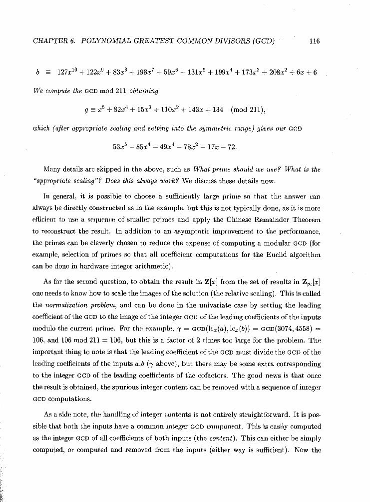
CHAPTER 6. POLYNOMIAL GREATEST COMMON DIVISORS (GCD) 116
b - 127x1•‹ + 1222' + 83x8 + 198x7 + 59x6 + 131x5 + 199x4 + 173x3 + 208x2 + 62 + 6
We compute the GCD mod 211 obtaining
g r x5 + 82x4 + 15x3 + 110x2 + 1432 + 134 (mod 211),
which (after appropriate scaling and setting into the symmetric range) gives our GCD
53x5 - 85a4 - 49x3 - 78z2 - 17x - 72.
Many details are skipped in the above, such as What prime should we use? What is the
"appropriate scaling"? Does this always work? We discuss these details now.
In general, it is possible to choose a sufficiently large prime so that the answer can
always be directly constructed as in the example, but this is not typically done, as it is more
efficient to use a sequence of smaller primes and apply the Chinese Remainder Theorem
to reconstruct the result. In addition to an asymptotic improvement to the performance,
the primes can be cleverly chosen to reduce the expense of computing a modular GCD (for
example, selection of primes so that all coefficient computations for the Euclid algorithm
can bc done in hardware integer arithmetic).
As for the second question, to obtain the result in Z[x] from the set of results in ZPi[x]
one needs to know how to scale the images of the solution (the relative scaling). This is called
the normalization problem, and can be done in the univariate case by setting the leading
coefficient of the GCD to the image of the integer GCD of the leading coefficients of the inputs
modulo the current prime. For the example, y = GcD(lc,(a), lc,(b)) = ~ ~ ~ ( 3 0 7 4 , 4 5 5 8 ) =
106, and 106 mod 211 = 106, but this is a factor of 2 times too large for the problem. The
important thing to note is that the leading coefficient of the GCD must divide the G c D of the
leading coefficients of the inputs a,b (y above), but there may be some extra corresponding
to the integer GCD of the leading coefficients of the cofactors. The good news is that once
the result is obtained, the spurious integer content can be removed with a sequence of integer
GCD computations.
As a side note, the handling of integer contents is not entirely straightforward. It is pos-
sible that both the inputs have a common integer GCD component. This is easily computed
as the integer GCD of all coefficients of both inputs (the content). This can either be simply
computed, or computed and removed from the inputs (either way is sufficient). Now the

CHAPTER 6. POLYNOMIAL GREATEST COMMON DIVISORS (GCD) 117
resulbing computed GCD should be integer content free, allowing removal of any spurious
integer content that is the direct result of the normalization scaling of the problem.
And now for the final question: Does this always work? The answer is no, and there are
two cases in which it may fail. One of these cases is dubbed the bad prime case, and the
other the unlucky prime case.
Definition 14 (Bad Prime) A prime p is bad if
deg,(GcD(a mod p, b mod p)) < deg,(g)
i.e. i j the degree of the GCD is too low.
Example 26 (Bad Prime) Consider the example problem, but perform the computation
modulo the prime 53. W e get:
Computing the GCD mod 53 gives:
g f x4 + 33x3 + 19x2 + 32% + 42 (mod 53),
which is of too low a degree.
The main problem with the bad prime case is that there is no way to scale the image
based on the leading coefficient estimate for the GCD, so the image cannot be used for
reconstruction via Chinese remaindering.
It is easily shown that a bad prime must divide the leading coefficient of the G ~ D .
Detection of the possibility that we have chosen a bad prime is dead simple. We need only
check the image of the scaling factor y modulo the chosen prime. If it is non-zero then the
prime is not bad. Note also that even if it is zero, then this does not guarantee that the
prime is bad, as it could divide the leading coefficients of both cofactors and not the leading
coefficient of the GCD, but detecting this is more difficult, so simply rejecting potentially
bad primes is a suitable approach.

CHAPTER 6. POLYNOMIAL GREATEST COMMON DIVISORS (GCD) 118
So given that the chosen prime is not bad, we can state that the computed GCD is at
worst a polynomial multiple of the true GCD. To detect that it is a true image of the required
GCD the chosen prime must not be unlucky.
Definition 15 (Unlucky Pr ime) A prime p is unlucky i f
deg,(GCD(a mod p, 6 mod p)) > 0,
i.e. if the degree of the GCD of the cofactors is not zero.
Example 27 (Unlucky Pr ime) Consider the example problem, but perform the compu-
tatiorl modulo the prime 13. We get:
a - 6x1•‹ + 9x9 + l l x8 + 5x7 + 21c6 + 7x5 + 11x4 + x3 + 5x2 + 22 + 9 (mod 13),
b r 8x1•‹ + 12x9 + 9x8 + 9x5 + 6x4 + 4x3 + 11x2 + 22 + 5 (mod 13).
So first we note that the prime is not bad, as it does not divide y = 106. Computing the
GCD rllod 13 gives
g-x6+8x5+2x4+6x3+9x2+11x+12 , (mod 13),
which is a problem, as we already know that our GCD should only be degree 5.
So in the example, the chosen prime 13 is unlucky. Unfortunately there is no efficient way
to detect an unlucky prime in advance. The general approach adopted by many algorithms
is to look for an image with too high a degree, relative to the other images, and often
includes a division check at the end (which can also be used to check for termination of the
algorithm).
This seems suitable as long as unlucky primes are not too plentiful, and this is made
clear by the following (simplified) lemma from Geddes [19]
Lemma 10 (Unlucky Primes) Let a, b be polynomials in Z[x] with GCD g and cofactors
a, b. Then p is an unlucky prime i f and only i f it divides the resultant r = res,(a, ?;).
Obtaining the resultant of the cofactors is much too expensive (for efficient computation
of a GCD) but this result does put a finite bound on the number of unlucky primes for a
specific problem, making the criteria described earlier sufficient for the task.

CHAPTER 6. POLYNOMIAL GREATEST COMMON DIVISORS (GCD) 119
For the example problem, the resultant is 1019581298696173769946 which factors as
(2) (3:') (13) (1452395012387711923), so there are only 4 unlucky primes for this problem.
Finally we will briefly describe some of the problems associated with computing GCDS
in more than one variable.
All the algorithms that follow at some point reduce multivariate problems to univariate
probloms by evaluation of the variables until a univariate problem is obtained. Alas the
unlucky and bad problems apply to the evaluation process in much the same way as they do
for primes in the modular process. This makes some sense, in that computing mod p, and
computing mod xi - ai are, loosely speaking, similar operations.
The extension for bad evaluations is fairly obvious; selection of a bad evaluation point
corresponds to choosing the evaluation so that the degrees of the polynomials in the remain-
ing variables drop. For example, in computing the GCD of (z + y - l)((y - l)x + 1) and
(x + ?j - 2)((y - 1)x + I) , which is (y - l ) x + 1, making the choice y = 1 will destroy the
GCD.
The extension for unlucky evaluations is similar. Selection of an unlucky evaluation
point corresponds to choosing the evaluation so that a GCD appears between the cofactors.
For example, in computing the GCD of the relatively prime polynomials x2 + y - 1 and
(y - 1)x2 + 1, the choice y = 2 could prove troublesome, as then both polynomials are
x2 + 1, making it appear as though they have a nontrivial GCD.
As with the bad prime case, the bad evaluution case is easy to avoid in advance, but the
unlucky evaluation case is not, so it is typically handled as an integral part of the algorithm.
The final problem we discuss is specific to lifting-based algorithms such as EEZ-GCD,
and it is called the bad zero problem. Lifting methods use the EEA to reconstruct variable
dependence. The lifting process only requires one of the GCD inputs, and attempts to
reconstruct the GCD and cofactor from the chosen input. In addition, only a single prime,
and a single evaluation of each variable are used throughout. For example, for a problem
with a = Gg, we would need to solve the EEA for a, T in
for a given value of c.
Now one requirement of the approach (for the EEA to work) is that the two factors in use

CHAPTER 6. POLYNOMIAL GREATEST COMMON DIVISORS (GCD) 120
(g and 6) must be relatively prime. If not, then c needs to be a multiple of G C D ( ~ , a) , which
is not always possible. Even if the initial g and 7i are relatively prime before evaluation, once
they are evaluated down to univariate polynomials, they may lose their relative primality.
Bofore we disregard this as being rare, we need to consider the following fact: lifting
based algorithms are significantly more eficient when the evaluation points are chosen t o be
zero. Unfortunately this is also the most common case where the relative primality is lost,
as zero evaluations remove terms from the problem inputs.
For example, consider the computation of a GCD where the form of a = 6g is (x3 + yz3)(:~;2 + yz). For this problem, the two input factors are relatively prime, but the primality
is losb if we evaluate any of the variables to zero.
The case where evaluating a variable to zero causes the two factors to have a common
GCD is called the bad zero problem.

CHAPTER 6. POLYNOMIAL GREATEST COMMON DIVISORS (GCD) 121
Givon problem in Z[xl, xn]
Problems in Zpi [XI ..,, xn] for i = l . . m
Desired solution in
Solutions in Zpi [XI, -.., xn] for i = l..m
1 Interpolate x,
1 4 Z Z - Y k 7 1 < 1 dx2 Interpolate x2
Problems in Solutions in
Figure 6.1: Homomorphism Diagram for Brown's Algorithm
6.3 Brown's Dense GCD Algorithm
Brown's description of the "dense modular GCD algorithm" in [8] is reproduced here for
the purpose of asymptotic analysis. Brown's algorithm has two subroutines, M and P.
The main subroutine M maps a polynomial GCD computation from Z[x] (or Z[xl, ..., xn])
into one or more GCD computations in Zp[x] for p E po,pl, . . ., and applies the Chinese
remainder theorem to obtain the solution in Z[x]. Brown's presentation of subroutine P is
similar. It maps a polynomial GCD computation from Zp[xn][xl, ..., ~ n - 1 1 into one or more
GCD computations in Zp[xl, ..., x,-~] by reducing the input polynomials modulo x, = a for
sufficiently many a E Zp, then recovers the dependence of xn by application of the Chinese
remainder theorem. ,
An important observation to make about Brown's algorithm is that both subroutines

CHAPTER 6. POLYNOMIAL GREATEST COMMON DIVISORS (GCD) 122
have been deliberately designed so that their termination does not require a trial division
o f th(: inputs by the GCD, nor multiplication o f the GCD and its cofactors t o verify that the
results are correct. This feature leads t o good performance for some GCD problems but poor
performance for others.
As hinted in the prior section, both algorithms will suffer from the bad and unlucky
prim(: and evaluation problems, and these are handled by the algorithms.
Algorithm 16 (Brown M, 1971)
Input: a,b E Z[x] \ {0), x = XI ,..., x,
1 Compute integer contents and their GCD.
Set ca = contx(a) E Z , a = alca, cb = contx(b) E Z , b = blca, and cg = G C D ( ~ ~ , cb).
2 Compute the correction coeficients.
Set la = lc,(a) E Z , lb = lcx(b) E Z , and y = ~CD(la,zb) .
3 Estimate bound for twice the height of y x g , y x ti, y x b as B = 2y max(1 la1 I,, I Ibl 1,). 4 Set m = 1 (the product of the moduli).
Set e = min(Axa, Axb) E Zn. Loop:
6 Choose a new prime p that does not divide la or lb.
7 Compute up = a mod p, bp = b mod p.
8 Compute gp,iip,bp E Zp[x] the monic GCD of up and bp and their cofactors using
algorithm P. If P fails (too few evaluation points are available) goto Loop.
9 Test for a , b relatively prime.
If Axgp = 0 then output cg, (ca/cg)a, (cb/cg)b.
10 If Axgp > e then (skip this unlucky prime) goto Loop.
11 Leading coeficient correction in Z .
Set gp = y x gp mod p.
12 First image? - -
If m = 1 then set g , = g,, Zi, = ti,, b, = bp, m = p, e = Axgp and goto Loop.

CHAPTER 6. POLYNOMIAL GREATEST COMMON DIVISORS (GCD) 123
13 I f Axgp < e then all previous primes were unlucky. Restart the algorithm keeping only
the current prime. . - -
Set g, = gp, a, = ap, bm = bp7 m = p, e = Axgp and goto Loop.
14 Combine the new image with the old using the C R A and express the result in the
15 Set m = m x p, i f m 5 B then goto Loop.
16 Test for termination.
Without explicitly computing g, x ti, and g, x 6 , determine if I lg, x tim/ 1, < m / 2
and)lg,x6,11, < m / 2 . I fsothenwehavemI(ya-g,x t i , ) a n d m I ( y b - g m x b m ) -
and also ya - g, x ti, = 0 and yb - g, x b, = 0 over Z , hence we are done; so -
set g = pp,(g,), S = lc,(g) E Z , a = ti,/S, b = b,/S.
Output cg x g, (ca/cg)ti, (cb/cg)b.
17 Goto Loop - either we do not have enough primes yet or all primes are unlucky.
Algorithm 17 (Brown P, 1971)
Input: a, b E Z [ x n ] [ x l , ..., x,-~] \ ( 0 ) ) p prime.
1 If n = 1 then compute the GCD using Euclid7s algorithm and the cofactors by division
and return, otherwise compute contents in Zp[xn] and their GCD.
Set ca = cant,, ,...,, ,-,(a) E Zp[xn] , a = a/ca,
cb = cont,, ,..., ,,-, (b) E Zp[xn] , b = blca, and cg = G C D ( C ~ , cb).
2 Compute the correction coeficients.
Set la = ~ C X ,,..., x,-, ( a ) E Zp[xn] , Ib = ~ C X , ,..., x,-l ( a ) E Zp[xn] , y = ~ c D ( l a , lb).
3 Bound the degree i n xn of y x g, y X 6, y x b. Set B = degXn y+max(d%,, a, degXn b).
4 Set m = 1 (the product of the moduli). Set e = m i n ( A x ,,..., ,,-,a, A, ,,..., ,,-, b) E zncl. Loop:
6 Choose a new evaluation point a E Z p such that x, - a does not divide la x lb. If no
such evaluation point exists then p is too small and the algorithm fails.

CHAPTER 6. POLYNOMIAL GREATEST COMMON DIVISORS (GCD)
7 Compute a, = a mod ( x , - a) E Z p [ x l , ..., xn-1]7 and
b, = b mod ( x , - a ) E Z p [ x l , ... , x,-11. -
8 Compute g,,Si,, b, E Z p [ x l , ..., x,-11 the monic GCD of a, and b, and their cofactors
with a recursive call to this algorithm.
9 Test for a , b relatively prime.
If Axl,...,xn-,g, = 0 then output cg, (ca/cg)a, (cb/cg)b.
10 If Axl,,..,xn-lg, > e then (skip this unlucky evaluation) goto Loop.
11 Leading coeficient correction in Zp[xn] .
Set g , = y ( a ) x g , mod p.
12 First image? -
If m = 1 then se tg , = g,, a, =a, , b, = b,, m = x , - a , e = Ax ,,.,,, xn-lga and
got0 Loop.
13 If Ax l , ,~~ ,xn- lg , < e then all previous evaluations were unlucky.
Restart the algorithm keeping only the current evaluation.
Set g, = g,, a, = a,, b, = b,, m = x, - a , e = Ax, ,..., xn-lgff and goto Loop.
14 Combine the new image with the old using the CRA.
Set a, = CRA([a,, a,], [x , - a , m ] ) , b, = CRA([b,, b,], [x , - a,m]),
gm = CRA([ga,gm], [ ~ n - a ,ml ) .
15 Set m = m x (x, - a) .
If degxn m 5 B then goto Loop.
16 Test for termination.
If deg,,, gm +degxn am = degxn y+degxn a and degxn gm +degxn bm = degxn y+degXn b
then set g = PP,, ,..., xn-, (gm)t 6 = lcxl ,..., ,,-,g, a = &/6, 6 = bm/6, and output cg x 9 ,
(ca/cg)~i , (cb/cg)6.
17 Goto Loop - all a's are unlucky.
In order t o determine the complexity o f Brown's algorithm, the central quantities o f
interest will be the number o f primes p used by algorithm M and the number o f evaluation
points a used by algorithm P. T h e reader will note that these quantities, computed in step
[3] and used in step 1151 o f both algorithms, are determined by the size o f the inputs a and
b and not by the size o f g, and 6.

CHAPTER 6. POLYNOMIAL GREATEST COMMON DIVISORS (GCD) 125
6.4 DIVBRO: The Modified Brown Algorithm
A modification of the Brown algorithm, DIVBRO, was presented by Monagan and Wittkopf
in [43], and provides greater efficiency for many classes of problems. It uses the well known
alternative of a division test to check for algorithm termination, and only constructs the
GCD, not the cofactors.
The new aspects of the approach that provide the increased efficiency are as follows:
Early Termination: Since we are only reconstructing g, we may need fewer primes in
algorithm M than required for reconstruction of g and the cofactors. In addition, the
bounds on the coefficient size of g are often pessimistic, forcing too many additional
images to be computed. If we apply the criteria that we perform the division check in
M once g is unchanged for an iteration, with high probability we need only perform
that division once, and we will compute a t most one extra image.
Degree Bounds: Since only the GCD is to be constructed, having reasonable bounds on
the degree of the GCD in XI, ..., x, can be used as a stopping criteria for algorithm P,
and helps with detection of unlucky primes and evaluations.
One-Pass Newton: Since we have degree bounds, the reconstruction of the current vari-
able in algorithm P can be done more efficiently, as we can perform the Newton
interpolation once all images have been computed, instead of reconstructing incre-
mentally.
Bivariate Optimizations: In the bivariate case, additional optimizations are available,
including a way to remove the division test in algorithm P and improved handling of
content computations for the GCD. These optimizations make a significant difference
for bivariate problems.
The details of the bivariate optimizations can be found in [43], but in this presentation
we are primarily concerned with the general multivariate case, so we will not discuss the
bivariate case further here. We present the modified algorithms below, where we note that
the numbering of the steps from Brown algorithms has been retained when possible (so the
numbering is not entirely sequential):

CHAPTER 6. POLYNOMIAL GREATEST COMMON DIVISORS (GCD)
Algorithm 18 (DIVBRO M)
Input: a,b E Z [ x ] \ {0 ) , x = X I ,..., x,
Output: g = G C D ( ~ , b)
1 Compute integer contents and their GCD.
Set ca = contx(a) E Z , a = alca, cb = contx(b) E Z , b = blca, and cg = G C D ( C ~ , cb).
2 Compute the correction coeficient.
Set la = lcx(a) E Z , ib = k x ( b ) E 2, and y = ~ c ~ ( l a , l b ) .
4 Set m = 1 (the product of the moduli).
Compute degree bounds e for the GCD in X I , ..., x,. Loop:
6 Choose a new prime p that does not divide y.
7 Compute up = a mod p, bp = b mod p.
8 Compute gp E Z p [ x ] the monic GCD of up and bp using algorithm P.
If P fails (too few evaluation points are available, or unlucky) goto Loop.
9 Test for a, b relatively prime: If Axgp = 0 then output cg.
11 Leading coeficient correction in 2 .
Set gp = y x gp mod p.
12 First image?
If m = 1 then set gm = gp, m = p, e = Axgp and goto Loop.
13 If Axgp < e then all previous primes and the degree bounds were unlucky.
Restart the algorithm keeping only the current prime and the new bounds.
Set g, = gp, m = p, e = Axgp and goto Loop.
14 Combine the new image with the old using the CRA and express the result in the
symmetric range for Z p .
set gm = CRA( [gp gml [P, m] )
15 Set m = m x p, and if g, changed in step 14 goto Loop.
16 Test for termination computing g = ppx(g,) and performing a division check to assure
that g divides both a and b. If so, we are done so output cg x g.
17 Goto Loop - either we do not have enough primes yet or all primes are unlucky.

CHAPTER 6. POLYNOMIAL GREATEST COMMON DIVISORS (GCD)
Algori thm 19 ( D I V B R O P )
Inpu t : a, b E Z [ x l , ..., x,-l] \ {0}, p prime, and the degree bounds eo.
O u t p u t : g = G C D ( ~ , b) or Fail
1
2
3
4
Loop:
6
7
8
10
9
11
12
13
If n = 1 then compute the GCD using Euclid's algorithm and return, otherwise compute
contents in Zp[xn] and their GCD.
Set ca = contxl ,..., xn- l (a) E Zp[xn], a = alca,
cb = cont,, ,..., ,,-, (b) E Zp[xn] , b = blca, and cg = GCD(CU, cb).
Compute the correction coeficient.
Set la = lcx ,,..., ,,-, ( a ) E Zp[xn] ) lb = 1cXl ,..., ,,-, ( a ) E Zp[xn] , y = GcD(la, lb).
Set the initial degree bounds for this computation, e = eo.
Set gSeq = Nul l , vseq = Nul l .
Choose a new evaluation point a E Z p such that x , - a does not divide y . If no such
evaluation point exists then p is too small, so return Fail.
Compute a, = a mod ( x , - a) E Z p [ x l , ..., 2,-11, and
b, = b mod ( x , - a) E Z p [ x l , ..., x,-11.
Compute g, the monic GCD of a , and b, with a recursive call to this algorithm.
If the recursive call fails (n > 2), or i f the GcD is of too high a degree (n = 2)
then (skip this unlucky evaluation) goto Loop unless this has occurred twice with no
successf211 images, in which case we assume that a higher prime or evaluation is unlucky
and return Fail.
Test for a , b relatively prime: If A,, ,..., ,,-,g, = 0 then output cg.
Leading coeficient correction in Z p [xn].
Set g, = ~ ( a ) x g, mod p.
First image?
If gseq = Nul l then set g,,, = g,, Useq = a, e = Ax, ,..., x,-lg, and goto Loop.
If Axl,..,,xn-lg, < e then all previous evaluations and the degree bound were unlucky.
Restart the algorithm keeping only the current evaluation.
Set gseq = g,, vseq = a, e = AX, ,..., x,-,g, and goto Loop.

CHAPTER 6. POLYNOMIAL GREATEST COMMON DIVISORS (GCD) 128
14 Add the new image and evaluation point
Set gseq = gseq, ga 9 Vseq = vseq, a
15 If we have enough images to construct to the degree bound in x , plus degzn(y) then
goto 18, otherwise goto Loop.
18 Compute the G c D g via Newton interpolation in x , using the sequence of GCDs gseq
und points useq.
19 Test for correctness
Remove the content g = pp n-l(gm) and check that g divides a and b. If so, output
cg x g, otherwise return Fail (unlucky content in x,).
Tlle main advantage of this approach is that the core computational complexity of the
algorithm is based on the coefficient size and the degree of g, unlike Brown's algorithm
which is based on the coefficient size and the degree of the inputs a and b.
6.5 Zippel's Sparse GCD Algorithm
Zippcl [78] proposed an algorithm (which can be used in combination with Brown's algo-
rithm) that is more efficient for sparse problems. The main idea behind this algorithm
is as follows: Once we know the form of the GCD for a specijc prime or evaluation, we
can use this information to more eficiently compute additional images for other primes or
evaluations.
Example 28 Consider the computation of the bivariate G c D x3 + 12xy + 100. Brown's P
algorithm would call Brown's M algorithm to compute the GCD g as
g = x 3 + 12xy2+9 (mod 13).
continuing to follow the Brown approach would require additional calls to Brown's M algo-
rithm to com,pute other images, say, mod 17, mod 23, etc.
The Zippel approach instead utilizes information about the form of the GCD obtained in
the first call assuming that the GCD is of the form x3 + axy2 + P for some a , P.
If this is the case, all information required for a new image mod 17 can be obtained from
a single univariate GCD call.

CHAPTER 6. POLYNOMIAL GREATEST COMMON DIVISORS (GCD) 129
The GCD is computed m o d ( y - 2,17) as x3 + 14x + 15, which is then equated to the
imayc of the assumed form of the G C D mod ( y - 2,17) as x3 + 4 a x + P, and we obtain
a - 12 mod 17, P r 15 mod 17, giving us the new image
g E x3 + 12xy2 + 15 (mod 17).
So as hinted at by the example, recursive calls t o compute new GCD images can be
replaced by the solution o f a sequence o f linear systems, and a bit o f manipulation.
Zippel's algorithm M is described here.
Algorithm 20 (Zippel M)
Input: a, b E Z[x] \ (0)
Output: g = G C D ( ~ , b)
1 compute integer GCD cg = G C D ( C O ~ ~ , ( ~ ) , cont,(b))
2 Compute the correction coeficient y = G C D ( ~ , ( ~ ) , k ,(b))
3 Estimate coeficient bound B = 2y m a ( / la1 I,, I lbl 1,) 4 Compute a modular GCD image gl with a call to the Zippel P algorithm for a random
prime pl .
5 Assume that of step 4 produces a correct image of the GCD with no missing terms, and
that the prime is not unlucky. W e call the assumed form gf. Count the largest number
of non-zero terms in any coeficient of the main variable X I , calling this n,.
7.1 Choose a new prime pi that it does not divide y.
7.2 Set S = 0, ni = 0
7.3 repeat
7.3.1 Choose a2, ..., a, E Z p at random such that deg,, ( a mod I ) = deg,, ( a ) , or
deg,, ( b mod I ) = degZl (b ) , where I = ($2 - aa, ..., x , - a,).
7.3.2 Compute gi = GCD(U mod I , b mod I ) .

C H A P T E R 6. POLYNOMIAL GREATEST COMMON DIVISORS (GCD) 130
7.3.3 Check if degxl (gi) < deg,, ( g j ) . If this occurs then our original image was
unlucky, so goto 4.
7.3.4 Check if degxl(gi) > degx,(gf). If this occurs then our current image is
unlucky, so goto 7.3.1.
7.3.5 Add the equations obtained from equating coeficients of gi and the evaluation
of gf mod I to S , and set ni = ni + 1.
Until ni 1 n,
7.4 W e should now have a suficient number of equations in S to solve for all un-
knowns in gf mod pi so attempt this now, scaling the leading coeficients of the
gi to y mod pi.
7.5 If the system is under-determined, then we need more images, so goto 7.3.1.
7.6 If the system is inconsistent, then our original image must be missing terms, or
the original prime was unlucky, so goto 4 .
7.7 The resulting solution is consistent and determined, so we have a new image gi,
so add to g,,, and add the prime to Pseq
Until we have a suficient number of primes to reconstruct our GCD to B.
8 Reconstruct our candidate GCD g using Chinese remaindering on gseq,pseq.
9 Perform a division test on g relative to the inputs. If it fails our original image must
be missing terms, or our original prime was unlucky, so goto 4.
10 return g.
Algorithm P can be easily obtained from algorithm M by replacing the coefficient bound
by a degree bound, the call to Zippel P by a recursive call in one fewer variable, and the
selection of new primes and evaluations mod a prime by the selection of new random values
vi for the current variable xj and evaluations mod ( 2 2 - 0 2 , .. . , xj- 1 - Q ~ - ~ , p) , where p is
the prime passed down from algorithm Zippel M.
A number of comments must be made on the above algorithm, most notably when and
why failures occur, and limitations of the algorithm.
The algorithm heavily depends on the completeness of the GCD image computed in step
2, where by completeness we mean that the image contains all the terms present in

CHAPTER 6. POLYNOMIAL GREATEST COMMON DIVISORS (GCD) 131
the GCD. It is straightforward to see that for a t term polynomial the probability that
a term may be missed is O(:) , where p is the current prime, and p >> t. This is not
such a restriction as long as either t is sufficiently small, or p is sufficiently large, but
can be a problem for a greater number of terms or small primes.
Bad results will always be detected by either the checks within the algorithm, or the
division test at the end, so if the algorithm returns a result it will be correct.
0 Thc termination of the algorithm depends upon the allowable choices of p, and the form
of the resulting GCD. If p >> t then the algorithm will likely terminate in the first pass,
while for p cx t the algorithm is unlikely to terminate.
Thc algorithm, as stated in [78], is only applicable to GcDs that are monic in the main
variable, which means the well known content and normalization problems are not
handled by this approach for the multivariate part (in Zippel P).
In the following section we will develop a modification of this algorithm that handles
the content and normalization problems, extending the algorithm to apply to a larger class
of problems.
6.6 LINZIP: The Modified Zippel Algorithm
In this section we will develop a modification of the Zippel sparse algorithm that is applicable
to all inputs in Z[xl, ..., x,].
The first problem we consider is the normalization problem. This is best illustrated
through a pair of examples, one of which is a straightforward modification, the other is not.
Example 29 Consider the computation of the bivariate GCD 3x3y2 + 12y + 100 at the top
level using the Zippel algorithm (20). In addition, we assume that we have y = 3, so we
know the leading coeficient of our GCD. The image obtained i n step 4 of the algorithm, with
pl = 13 would be
g - x3y2 + 4y + 3 (mod 13),
so our expected form of the GCD , after scaling through by y , is gf = 3x3y2 + ay + P .

CHAPTER 6. POLYNOMIAL GREATEST COMMON DIVISORS (GCD) 132
Siuce the O(xO) term has two terms, we need to compute two modular images for our
next prime to reconstruct the y dependence. For the next prime, p2 = 17, we choose y = 1,2
and obtain the GCDS x3 + 9 and x3 + 16 respectively.
Before converting to a linear system we need to normalize the computed GCD, as other-
wise blie linear relations will give an incorrect result. Fortunately this is easy to do here, as
we know the form of the leading coeficient, including the y dependence, which is 3y2. As
a result we must scale our first univariate GCD by 3(1)~ = 3, and the second b y 3(2)2 = 12
beforc equating, giving:
1 2 ~ ~ + 2a + @ = 12x3 + 5
Solving this system for a, @ mod 17 gives a = 12, @ = 15 resulting in the new image
g2 -- 3x3y2 + 12y + 15 (mod 17).
Additional images for other primes can be computed in the same way.
So for a coefficient known up to a scaling there is no problem. What is interesting is
what occurs when we can no longer scale a single coefficient of the GCD for reconstruction,
as illustrated by the next example.
Example 30 Consider the computation of the bivariate GCD ~ ~ ( 3 ~ ~ - 90) $ 12y i- 100 at
the top level using the Zippel algorithm (20). The image obtained in step 2 of the algorithm,
with pl = 13 would be
gl = x3y2 + 9x3 + 4y + 3 (mod 13),
so our expected form of the GCD is gf = x3y2 + ax3 + py + y. Since each x term of the GCD has two terms, we need to compute two modular images
for our next prime to reconstruct the y dependence. For the next prime, pz = 17, we choose
y = 1,2 and obtain the GCDS x3 + 12 and x3 + 8 respectively.
Now we run into a problem when attempting to normalize the computed GCDS to construct
the linear system we require. The dificulty is this: All coeficients of the GCD have unknown
parameters present, so we have no way of scaling the GCD unless we know the exact form of
one of the coeficients.

CHAPTER 6. POLYNOMIAL GREATEST COMMON DIVISORS (GCD) 133
A solution to the problem illustrated by the above example could be obtained in a number
of ways. One approach involves computation of one of the required coefficients exactly, for
example by factoring the leading coefficient, as is done by the EEZ-GCD algorithm. We
wish to avoid this as it could be expensive, and it complicates the implementation of the
algorithm.
This problem only occurs when all coefficients of the GCD with respect to the main
variable have more than one term. In any other case, we can choose any single term
coefficient to use for scaling (not just the leading or trailing coefficient) as the form of single
term coefficients is always known up to a scaling of the entire GCD.
It is clear that the problem boils down to how to scale the univariate GCD images in
such a way that the solution of the linear system produces the correct result.
Tlie approach followed now is quite simple in concept. It is to treat the scaling factors of
the computed univariate GCDS as unknowns as well. This results in a larger linear system,
and sometimes requires additional univariate GCD images, but never requires additional
multivariate GCD computations. We call this the multiple scaling case (as opposed to the
single scaling case).
If we allow all univariate GCDS to be scaled along with all coefficients of the assumed
form of the multivariate GCD, the resulting system will be under-determined by exactly 1
unknown, as the computation is only determined up to a scaling factor. Rather than fixing
an unknown in the form of the GCD to 1, we instead fix the scaling factor of the first GCD to
I (for reasons to be explained later).
Tlie following example illustrates this approach.
Example 31 Consider the computation of the bivariate GCD from Example 30:
(3y2 - 90)x3 + 12y + 100. Just as i n that example, we obtain for p l = 13
g z x3y2 + 9x3 + 4y + 3 (mod 13),
and expected form of the GCD g j = ax3y2 + Px3 + yy + a.
Instead of computing two univariate GCD images for the new prime p2 = 17, we compute
three, choosing y = 1,2,3 and obtaining the GCDS x3 + 12, x3 + 8, and x3 respectively. W e

CHAPTER 6. POLYNOMIAL GREATEST COMMON DIVISORS (GCD)
form the modified system as follows:
when: m2,m3 are the new unknown scaling factors, and we have set the first scaling factor
ml to 1.
Solving this system yields a = 7,P = 11, y = 11,a = 1, with scaling factors m2 =
5, m3 = 6, so our new GCD image is given by
g =- 7x3y2 + 11x3 + l l y + 1 (mod 17),
which is consistent with our GCD.
Now we explain the reason for fixing a multiplier value instead of an unknown in the
GCD. In general it is possible to select a prime or evaluation so that the chosen scaling term
in the GCD is zero, but there is no way to detect it. For the example, suppose we set a = 1.
In this case, the evaluation y = 0 is not bad (the form of the GCD is still cubic in x) but
a = 0, so the resulting system will be incorrect. Attempting to set P = 1 will have the
same problem if we used the prime p = 5. In contrast, as long as we choose our primes and
evaluations so that the leading term of the GCD does not vanish (which is detected as a bad
primc or evaluation), then the scaling factors can never be zero, so setting one of them to
a fixed value will never result in this problem.
One might wonder why the multiple scaling case can be even mildly efficient, as we are
constructing a system that ties together all unknowns of the problem through the multipliers.
This is in direct contrast to the single scaling case, for which each degree in XI has an
independent subsystem. The trick is to realize that the resulting system is highly structured,
and the structure can be exploited to put the solution expense of the multiple scaling case
on the same order as the solution expense of the single scaling case.
Example 32 (Multiple Scaling) Consider the linear algebra required in the computation
of the GCD for a problem with the image:

CHAPTER 6. POLYNOMIAL GREATEST COMMON DIVISORS (GCD) 135
We find that we will have a suficient number of equations to solve for all unknowns if we
compute 4 images, where we note that for this problem the number of required images is
exactlg the same as for the single scaling case. The resulting Matrix, involving 16 equations
for th,e 15 unknowns (12 image unknowns and 3 unknown scaling factors) has the following
structure:
Where the equations are ordered by decreasing degree in x then by image number, and the
unknowns are ordered in the same order as the image, with the scaling factors on the right,
and the c's denote (possibly) non-zero entries, all other entries being strictly zero. Note also
that the first column of multipliers (the bold c's) have fixed values.
The solution of the above system can be easily computed by solution of a number of
smaller subsystems corresponding to the rectangular blocks of non-zero entries augmented
with the multiplier columns. Once the subsystems are upper triangular, remaining rows,
only involving the multipliers, can be used to compute the multiplier values, which can then
be back-substituted into the subsystems to obtain the image coeficients.
Note that for the single scaling case, the structure is similar to the above, except that the
scaling columns would be replaced by a single column of constants. For that case, all blocks
are clearly independent, making the eficient solution of the problem obvious.
This approach does offer a solution to our problem, but it also introduces another diffi-
culty, as illustrated by the following example:

CHAPTER 6. POLYNOMIAL GREATEST COMMON DIVISORS (GCD) 136
Example 33 Consider the computation of the bivariate G c D (y + 2)x3 + 1 2 ~ ~ + 24y. Using
a call to the Brown algorithm, we can obtain our first image for pi = 13 as
gl = x 3 ~ + 2 x 3 + 12y2 + l l y (mod 13),
and expected form of the GCD gf = ax3y + Px3 + y i2 + ay.
J w t as for the prior example, we know we need at least three univariate G c D images for
the new prime pz = 17. W e choose y = 1,2,3 and obtain the GCDS x3 + 12, x3 + 7, and
x3 + 2 respectively. We form the modified system as follows:
ax3 + px3 + y + a = x3 + 12,
2ax3 + ,8x3 + 47 + 20 = m2 (x3 + 7),
3ax3 + Px3 + 97 + 3a = m3(x3 + 2),
In attempting to solve this system, we find that it is under-determined, so we add a new
evaluation point, y = 4, obtaining a GCD of x3 + 14, and the new equation
In attempting to solve the new system of equations, we find that it is still under-determined.
In fact, we could continue to choose new evaluation points for y until we run out of points
(modp) , and the linear system would remain under-determined.
This is the case for any chosen prime and set of evaluations, so the algorithm fails to
find the GCD for this problem.
What is not necessarily obvious from the above example is the cause of the failure, which
is the presence of a content in the GCD with respect to the main variable x, namely y + 2.
The existence of a content in the evaluated variables can be immediately recognized as a
source of problems for the algorithm, as it can be absorbed into the multipliers on the right
hand side of the formed system for the equations with multipliers, and otherwise absorbed
into each of the unknowns (for the first equation where the multiplier is set to 1).
This is exactly what occurs in the above example, as the content in y is absorbed into
the unknowns, so only the relative ratio between terms can be computed, and we can never
obtain a solution for the coefficients in our candidate form.

CHAPTER 6. POLYNOMIAL GREATEST COMMON DIVISORS (GCD) 137
It is clear that content can cause a problem for the algorithm, so just as for many
other sparse algorithms (EEZ-GCD for example), the content must be removed before the
algorithm is called.
Hore we note that the content removal problem has been dealt with in a very elegant
fash io~~ in Kaltofen and Trager 1331, wherein a transformation of the form xi H xl + cuxi for
random a and 2 5 i < n is applied to the input polynomials to force the content to become
part of the GCD in the main variable. We also note that efficient use of this technique
requircs treatment of the input polynomials as black boxes, as otherwise the polynomials
become dense, and as we are focusing on direct modular techniques, where such a technique
would result in excessive expression swell, we discuss this approach no further here.
Olie may ask is it suficient to simply remove the GCD content before calling the algorithm
to takc care of this problem? Unfortunately, the answer is no, as certain choices of primes
and evaluation points can cause an unlucky content to appear in the GCD.
Definition 16 (Unlucky Content) Given a E Z[xl, ..., x,] with cont,, ( a ) = 1, a prime p
is said to introduce an unlucky content i f cont,, ( a mod p) # 1. Similarly for a E Z[xl, ..., x,]
with cont,,(a) = 1 an evaluation X i = ai is said to introduce an unlucky content if
cont,, (a mod (xi - ai)) # 1.
Consider, for example, computation of the GCD x(y+ 1)+y+14. If we choose p = 13 the
GCD has a content of y + 1, while for any other prime, or over Z[x, y], no content is present.
This is a significant consideration in the design of the algorithm, and must be carefully
checked. An argument can be made as to the similarity between the probability of obtaining
an unlucky content, and the probability of selecting an unlucky prime or evaluation, and the
fact that these are both equally uncommon, so a similar approach will be used in the design
of the algorithm for handling unlucky contents. Specifically we will design the algorithm so
these problems are not detected in advance, but rather through their effect, so that detection
of this problem does not become a bottleneck of the algorithm.
We now present the LINZIP M algorithm, which computes the GCD in Z[x] from a
number of images in Zp[x], and the LINZIP P algorithm, which computes the GCD in
Zp[xl, .. . , x,] from a number of images in Zp [xl, . . . , x,-~]. We emphasize that any content
of the GCD with respect to x l must be removed before the initial call to the LINZIP M

CHAPTER 6. POLYNOMIAL GREATEST COMMON DIVISORS (GCD)
algorithm, though it is not required that the cofactor contents be removed.
Algorithm 21 (LINZIP M)
Input: a,b E Z[x] such that ~~~(cont,,(a),cont,,(b)) = 1 and degree bounds dx on the
GCD in X
Output: g = G C D ( ~ , b) E Z[X]
1 Compute the scaling factor y = G C D ( ~ , ( ~ ) , lcx(b)) E Z
2 Choose a random prime p such that yp = y mod p # 0 , and set a, = a mod p,
bp = b mod p, then compute from these a modular GCD image gp E Z p [ x l , ..., x,] with
a call to LINZIP P. If the algorithm returns Fail, repeat, otherwise set d,, = deg,, (gp)
and continue.
3 Assume that g, has no missing terms, and that the prime is not unlucky. W e call the
assumed form g j . There are two cases here.
3.1 If there exists a coeficient of x l in gf that is a monomial, then we will normalize
by setting the integer coeficient of that monomial to 1. Count the largest number
of terms in any coeficient of x l in g f , calling this n,.
3.2 If there is no such coeficient, then multiple scaling must be used. Compute the
minimum number of images needed to determine gf for a new prime with multiple
scaling, calling this n,.
4 Setg,= - x g P m o d p a n d m = p .
5 Repeat
5.1 Choose a new random prime p such that yp = y mod p # 0 , and
set a p = a m o d p , bp = b m o d p .
5.2 Set S = 0, ni = 0.
5.3 Repeat
5.3.1 Choose az, ..., a, E Z p at random such that for I = ( x 2 - a2, ..., x , - a,)
we have degXl (a, mod I ) = deg,, ( a ) , deg,, (b, mod I ) = deg,, (b), and set
a1 = a, mod I , bl = bp mod I
5.3.2 Compute gl = G C D ( ~ ~ , b l )

CHAPTER 6. POLYNOMIAL GREATEST COMMON DIVISORS (GCD) 139
5.3.3 If degx,(gl) < d,, then our original image and form g f and degree bounds
were unlucky, so set d,, = deg,, ( g l ) and goto 2.
5.3.4 I f degxl(gl) > d,, then our current image is g l unlucky, so goto 5.3.1, un-
less the number of failures exceeds min(1, n,), in which case we assume p is
unlucky and goto 5.1.
5.3.5 Add the equations obtained from equating coeficients ofgl and the evaluation
of gf mod I to S , and set ni = n, + 1.
Until ni > n,
5.4 We may now have a suficient number of equations in S to solve for all unknowns
in g f mod p so attempt this now, calling the result gp.
5.5 If the system is inconsistent then our original image must be incorrect (missing
terms or unlucky), so goto 2.
5.6 If the system is under-determined, then record the degrees of freedom, and if
this has occurred twice before with the same degrees of freedom then assume that
an unlucky content problem was introduced by the current prime p so goto 5.1.
Otherwise we need more images so goto 5.3.1.
5.7 The resulting solution is consistent and determined, so we have a new image gp Y
Set gp = lcx&p) x gp mod^, gm = CRA([gp,gml,lp,ml), m = m x P.
Until g, has stopped changing for one iteration.
7 Compute g, = pp,(gm) and check that g, I a and g, I b. If not we need more primes,
so goto 5.1.
8 Return g,.
Algorithm 22 (LINZIP P)
Input: a, b E Z p [ x l , ..., x n ] , a prime p, and degree bounds d, on the G C D in x
Output: g = GCD(U, b) E Z p [ x l , ..., xn] or Fail
0 Check the GCD of the inputs for content in x,, zf present return Fail.
1 Compute the scaling factor 7 = G C D ( ~ C ~ , , . . . , ~ ~ - , ( a ) , l ~ x , , . . . , ~ ~ - , (b ) ) E Zp[xn]
2 Choose v E Z p at random such that deg, ,,.,., xn-,(a mod ( x , - v ) ) = deg, xn-,(a),
deg,, ,..., xn-, (b mod ( x n - v ) ) = degx, ,..., X n - , (b) , and set a, = a mod (xn - v ) , bv =

CHAPTER 6. POLYNOMIAL GREATEST COMMON DIVISORS (GCD) 140
1) mod ( x , - v ) , then compute from these a modular G C D image g, E Z p [ x l , ..., x,-~] with a recursive call to LINZIP P (n > 2) or via the Euclidean algorithm (n = 2).
If for n > 2 the algorithm returns Fail or for n = 2 we have deg,, (g,) > d,, then
return Fail, otherwise set d,, = deg,, (g,) and continue.
3 Assume that g, has no missing terms, and that the evaluation is not unlucky. We call
the assumed form g f . There are two cases here.
3.1 If there exists a coeficient of xl in gf that is a monomial, then we will normalize
by setting the integer coeficient of that monomial to 1. Count the largest number
of terms in any coeficient of x l in g f , calling this n,.
3.2 If there is no such coeficient, then multiple scaling must be used. Compute the
minimum number of images needed to determine gf for a new evaluation of x ,
with multiple scaling, calling this nx.
Y Set g w = lc,, ,..., :n:l (&) x g, mod p and vseq = V .
5 Repeat
5.1 Choose a new random v E Z p such that degxlt..,xn-l ( a mod ( x , - v ) )
= d%Xl ,..,xn-l ( a ) 7 degxl,.., xn-1 (b mod ( x n - v ) ) = degx,,..,xn-, (b) , and set a, = a mod ( x , - v ) , b, = b mod ( x , - v).
5.2 Set S = 0, ni = 0.
5.3 Repeat
5.3.1 Choose a2, ..., a,-1 E Z p at random such that for I = ( x 2 - a2, ..., 2,-1 -
an-1) we have deg,, (a, mod I ) = deg,, ( a ) , deg,, (b, mod I ) = deg,, (b) ,
and set a1 = a, mod I , bl = b, mod I
5.3.2 Compute $1 = G C D ( U ~ , bl)
5.3.3 If deg,,(gl) < d,, then our original image and form gf and degree bounds
were unlucky, so set d,, = deg,, ( g l ) and goto 2.
5.3.4 If deg,, ( g l ) > dxl then our current image is gl unlucky, so goto 5.3.1, unless
the number of failures exceeds min(1, ni), in which case we assume x , = v is
unlucky and goto 5.1.
5.3.5 Add the equations obtained from equating coeficients of gl and the evaluation
of gf mod I to S , and set ni = ni + 1.

A number of comments are required for the above algorithms, and a discussion of the
correctness and termination of the overall algorithm follows.
1. The degree bounds of the GCD have very specific uses. The degree bound of the GCD in
the main variable xl is used to detect unlucky primes and evaluations, but only detects
those that involve 21, and we update the degree bound whenever we compute a GCD of
lower degree in XI. The degree bounds of the GCD in the non-main variables 2 2 , ..., x,
are used to compute the number of images needed in the Newton interpolation in step
6 of L I N Z I P P, and are not updated by the algorithm.
CHAPTER 6. POLYNOMIAL GREATEST COMMON DIVISORS (GCD)
Until ni 2 n,
5.4 W e should now have a suf ic ient number of equations in S to solve for all un-
knowns in g f mod p so attempt this now, calling the result gv.
5.5 I f the system is inconsistent then our original image must be incorrect (missing
terms or unlucky), so goto 2.
5.6 If the system is under-determined, then record the degrees of freedom, and if
this has occurred twice before with the same degrees of freedom then assume the
content problem was introduced by the evaluation of x, so goto 5.1. Otherwise
we need more images so goto 5.3.1.
5.7 The resulting solution is consistent and determined, so we have a new image g, 7 v
Set gseq = gseq, iczl ,..., L,), (9,) x gv, vseq = vseq, v
Until we have d,, + degXn (y) + 1 images.
6 Reconstruct our candidate GCD g, using Newton interpolation (dense) o n gs,g,v,eq,
then removing content in x,.
7 Loop some fixed number of t imes
7.1 Choose a 2 , ..., a, E Z p at random such that I = (x2 - a 2 , ..., x, - a,) is not a
bad evaluation point, and set a1 = a mod I , bl = b mod I , and g, = g, mod I .
7.2 Compute gl = G C D ( U ~ , bl) and if gl does not divide g, then our original image
mus t be bad, so goto 2.
8 Return g,.

CHAPTER 6. POLYNOMIAL GREATEST COMMON DIVISORS (GCD) 142
2. The number of required images for the multiple scaling case computed in step 3.2 can
be the same as the number of required images for the single scaling case computed in
step 3.1 (if the GCD is of certain forms), and up to a t most 50% higher. The worst
case is quite infrequent, and will only occur when there are only two coefficients with
respect to the main variable, each having exactly the same number of terms. For three
coefficients, this is limited to 33%) for 10 it is limited to lo%, etc. The extra expense
of this step can usually be reduced by an intelligent choice of the main variable XI.
The exact formula for the number of images needed depends upon the term counts
for a problem. For a problem with coefficients having term counts of n l , ..., n, for
the coefficients with respect to XI and a maximum term count of nmax is given by
1nax(nmax1 T(Ci=l ni - l) /(s -
3. T11c check in step 0 of LINZIP P is used to detect an unlucky content in the initial
GCD introduced higher up in the recursion by either a prime or evaluation. Note that
we can always detect the problem (if not the source of the problem) in this way, as any
content in the GCD with respect to XI will eventually show up as a univariate content
as we evaluate x,, x,-1, ....
4. The check in step 5.6 of either algorithm is intended to check for an unlucky content
introduced by the evaluation (LINZIP P) or prime (LINZIP M) chosen in step 5.1 of
both algorithms. Since it is possible that a new random image from step 5.3.1 does
not necessarily constrain the form of the GCD (even without the content problem) we
check for multiple failures before rejecting the current iteration of loop 5.
5. The LINZIP P algorithm has been modified to perform a probabilistic division test in
step 7 instead of testing that g, I a and g, I b. If a few iterations are performed, then
the result is correct with high probability, and the test is substantially less expen-
sive. There is, however, a chance that the test fails to detect an incorrect answer, so
the termination division test in LINZIP M must be retained to make the algorithm
deterministic.
6. A major enhancement could be realized through the use of a highly efficient implemen-
tation of Brown's P algorithm once we evaluate down to 2 variables. The reasoning
here is that by the time we evaluate down to 2 variables, the problem will very likely
be dense in those variables. In this case, the use of the Brown approach could provide

CHAPTER 6. POLYNOMIAL GREATEST COMMON DIVISORS (GCD) 143
an efficiency improvement, and if implemented as a general strategy (i.e. always eval-
uate down to a bivariate problem instead of a univariate one), would make the use
of multiple scaling less likely (as now we are considering coefficients with respect to 2
variables), and would reduce the size of the linear systems to be solved.
7. There is an enhancement to the above algorithm that is not explicitly described, and it
is the following: Do not always throw away images when repeating step 2 as the result
of an inconsistent system in step 5.5. Instead retain the image, and consider it with
respect to the new computed image. If the images differ with respect to relatively few
terms, then use them both to determine the expected form for g. Note that this is
typically the main failure case for the algorithm (i.e. it has a much higher probability
than an unlucky prime/evaluation or an unlucky content). This has the advantage
that even for problems where the number of terms is close to the value of the prime,
all terms of the image will eventually be found, and in the unlikely event that one of
the images chosen for use was unlucky, this will only enlarge the number of terms to
be solved for, and will not result in an incorrect solution.
We now discuss the correctness and termination of the algorithm. We need to consider
4 main problems with sparse modular methods, namely bad primes or evaluations, unlucky
contents, unlucky primes or evaluations, and missing terms (in an initial image).
The treatment of bad primes and bad evaluations is straightforward, and is handled for
the first prime or first evaluation by the vector degree checks in step 2 of the algorithms,
handled for the current prime or current evaluation by the vector degree checks in step 5.1
of the algorithms, and handled for the univariate images in step 5.3.1 of the algorithms.
The treatment of the unlucky content problem for the first prime or first evaluation is
handled in step 0 of LINZIP P by the single variable content check. As in point 3 above
we emphasize that this check will always detect the problem at some level of the recursion,
specifically the level containing the last variable contained in the unlucky content (as all
the other variables in the content have been evaluated, so the content becomes univariate).
We note that there is no efficient way to detect which prime or evaluation introduced the
unlucky content. It may have been introduced by the prime chosen in LINZIP M or any
evaluation in prior calls (for x3 with j > n) to LINZIP P in the recursion. Since this
problem is rare, we handle this by rejecting the case all the way back up to the LINZIP M

CHAPTER 6. POLYNOMIAL GREATEST COMMON DIVISORS (GCD) 144
algorilhm, which results in a completely new prime and set of evaluations. This strategy is
fairly efficient, as only evaluations (modular and variable) and other single variable content
checks have been performed before a failure is detected at any level of the recursion.
The introduction of an unlucky content by the prime or evaluation chosen in step 5.1
of eitller algorithm will be handled in the combination of steps 5.4 and 5.6. Note that an
unlucky content is only a problem when multiple scaling is in use (as it is the scaling of
the image that is the issue). The result is a system with additional degrees of freedom, so
this always results in an under-determined system. The check in step 5.6 handles this, as
eventually we will obtain a solution for all variables but the free ones resulting from the
unlucky content, so the degrees of freedom will stabilize, and we will go back to step 5.1
choosirlg a new prime or evaluation.
The treatment of unlucky primes is less straightforward.
First we consider an unlucky evaluation in step 2 of LINZIP P for x, for which the
factor added to the GCD depends upon XI. If the degree bound dxl is tight, then this will
be dctected at a lower level of the recursion by step 2 of LINZIP P when n = 2. If the
degrec bound dxl is not tight, then the G c D computed in that step may be unlucky, but we
proceed with the computation. Once we reach loop 5, we begin to choose new evaluation
points for x,, and with high probability we will choose a new point that is not unlucky
in step 5.1, the problem will be detected in step 5.3.3, and we will go back to step 2, and
compute a new image. In the worst case, all evaluations in step 5.1 may also be unlucky,
introducing the same factor to the GCD, and we will proceed to step 6, and reconstruct an
incorrect result. Note that if the factor is in fact different, then the equations accumulated
in step 5.3.5 will most likely be inconsistent, and this problem will most likely be detected
in steps 5.4 and 5.5. Step 7 will again perform checks much like those in step 5.3.3, and
will detect this problem with high probability, but if it does not, an invalid result may be
returned from LINZIP P.
If we continue to choose unlucky evaluations we will eventually return an incorrect image
to LINZIP M.
This problem (as well the unlucky prime case for step 2 of LINZIP M) is handled by
the structure of the LINZIP M algorithm. Since the steps are essentially the same, the
same reasoning follows, and we need the computation to be unlucky through all iterations

CHAPTER 6. POLYNOMIAL GREATEST COMMON DIVISORS (GCD) 145
of loop 5. Now in this case, since the form of the GCD is incorrect, it is unlikely that g, will
stabilize, and we will continue to loop. Note that in the event that g , does stabilize, the
invalid image will not divide a and b, so step 7 will put us back into the loop. Now within
that loop, which will not terminate until we have found the GCD, step 5.3.4 will eventually
detect this problem, as we must eventually find a prime that is lucky.
So the unlucky case for the initial image is handled when the factor added to the
GCD dcpends upon XI.
Now consider the case where the unlucky evaluation or prime is chosen in step 2 of either
algorithm, and the factor added to the GCD is independent of XI. In this case, the factor is
actually a content with respect to X I , so this is handled by the same process as the unlucky
content problem, specifically it is handled on the way down by step 0 of LINZIP P.
Now if an unlucky prime or evaluation occurs in step 5.1 of either algorithm, it will either
raise the degree in XI, in which case it will be detected in step 5.3.4 of either algorithm,
or it will be independent of XI, in which case it is a content. If the content is purely a
contribution of the cofactors, then this case will not cause a problem for the algorithm, as
it will simply reconstruct the new GCD image without that content present (as a result of
the assumed form).
The only type of unlucky evaluation that can occur in step 5.3.1 of either algorithm
must raise the degree of the GCD in XI, so is handled by step 5.3.4.
The final issue to discuss is the case where the initial image is missing terms in either
algorithm. When this occurs, the resulting system will likely be inconsistent, so will be
detected by step 5.5 with high probability, but this may not be the case. If the problem is
not detected in any iteration of loop 5, then an incorrect image will be reconstructed in step
6 of LINZIP P. The additional check(s) in step 7 of LINZIP P will, with high probability,
detect this problem with the new images, but if this also fails, then we return an incorrect
image from LINZIP P.
Again assuming a sequence of failures to detect this problem, we arrive at LINZIP M.
Now we will compute new images in LINZIP M until g , divides both a and b, so the problem
must eventually be detected.
Note that the missing term case is the most likely failure case, as unlucky primes, unlucky
evaluations, and unlucky contents are generally quite unlikely. The probability of choosing

CHAPTER 6. POLYNOMIAL GREATEST COMMON DIVISORS (GCD) 146
a prime or evaluation that causes a term to vanish is O( i ) , where t is the number of terms
in thc polynomial, and p is the prime. So for sparse problems, and a sufficiently large prime,
the chance of a bad evaluation is small, and the initial image is likely not missing terms.
Convctrsely if the prime is small, or the problem is large and dense (having many terms), it
is possible that the algorithm may never terminate. The algorithm, however, is designed for
spars(! problems, so this is not an issue as long as primes of a suitable size are used. Note
that the enhancement described as item 7 earlier can be used for this case.
6.7 The EEZ-GCD Sparse GCD Algorithm
The EEZ-GCD algorithm is also based on modular computation, though it takes a distinctly
differont approach than the methods described thus far. To understand the method, it is
necessary to lay some foundations for the padic and I-adic lifting methods.
The information in this section is provided primarily to give the flavor of the method,
and the details for efficient implementation of the algorithms are left for the asymptotic
analyses.
6.7.1 Lifting Methods
The basic approach used in these lifting methods is to pose the problem in the form of an
equation, f (u) = 0, where u E Z[xl, ..., x,], and obtain a solution ul in a simpler domain
Zp[xl] such that u1 satisfies f (ul) = 0 mod (p, xz - a a , ..., x, - a,). The solution UI is then
lifted to the solution u E Z[xl, ..., xn].
A generic description of a lifting process (that parallels the one in use by EEZ-GCD) is
presented in the following diagram:
There are some significant differences between this approach and the modular approaches
described earlier.
1 This approach performs only one computation of the actual problem in the simpler do-
main, Zp[xl], then uses that solution to reconstruct the solution of the full problem.
2 Only one prime and set of evaluations is used for the entire process.

CHAPTER 6. POLYNOMIAL GREATEST COMMON DIVISORS (GCD)
Desired solution in Zpl[xl, -, xn]
I Lift x2
Solution in Zpl [XI]
Lift to p1
Problem in Solution in
Figure 6.2: Homomorphism Diagram for Lifting Approach
3 Thc integer coefficient reconstruction is performed at the lowest level, before
tion of the dependence of the variables 22, .. . , x,. reconstruc-
Note that 1 is chosen to be sufficiently large so that the solution in Zpl is the same as
the solution in Z. The lifting process for the variables can proceed one variable at a time,
or all variables simultaneously.
6.7.2 Application to GCD (p-adic lifting)
The lifting approach utilized to compute GCD is known as Hensel lifting, and is slightly
different than the lifting process described in the prior subsection.
The equation to be solved depends upon two expressions, u, w, and is of the form F -

CHAPTER 6. POLYNOMIAL GREATEST COMMON DIVISORS (GCD) 148
uw = 0, where F E Z[xl , ..., x,] is one of the polynomials for which we are computing the
GCD, and u, w are the G c D and cofactor of that polynomial.
With this in mind, the first step, finding the solution in Zpl [xl] (effectively in Z[xl]), is
simply the process of evaluating the polynomial inputs at (p, x2 - a 2 , .. . , x, - a,), computing
the GCD ul , then selecting F to be one of the polynomials, and wl to be the corresponding
cofactor. We then lift the solution to one with coefficients in Z by applying univariate
Hensel lifting which we give a basic description of below.
Note we are free to choose either of the polynomial inputs as the one used in the recon-
struction, which allows us some flexibility that can be leveraged to increase the efficiency of
the algorithm.
To see how the univariate Hensel lifting algorithm works, we re-write u, w, F for the
problcm in Z[xl] in p-adic form (base p) as follows
where ui, wi, F' E Zp[xl].
Now consider the equation we want to solve, F - uw = 0. Application of the re-written
forms above gives
from which it is obvious (by considering the equation mod p) that the O(pO) term is satisfied
immediately by setting u0 = u1 and w0 = wl.
We then want to improve the approximation by computing higher order terms, namely
ul , wl, u2, w2, . . . , requiring that
F - (uO + ulp + ... + uipi)(wO + wlp + ... + wipi) r 0 (mod pi").
We will label these improved approximations ui, defining these as ui+l = ui + uipi, with a
similar definition for w.

CHAPTER 6. POLYNOMIAL GREATEST COMMON DIVISORS (GCD) 149
Wc will assume the use of l inear lifting to obtain the higher order terms, and not quadratic
lifting. Using l inear lifting we obtain a single higher order term (such as u1,u2, ...) in each
step. Use of quadratic lifting allows doubling the number of known higher order terms in
each step, but the computations in each step are more expensive, and the overall cost is
shown to be asymptotically equivalent by Miola and Yun [41], assuming that classical integer
multiplication and division are used.
Wo assume that we have computed ui, wi and show how to obtain ui, wi, thus obtaining
the approximations ui+l, wi+l.
By definition, we have:
F - u i w i - 0 (rnodpi).
Now consider the exact solutions u,w:
Substitution into our equation F - uw, computing mod pi+' gives
F - (ui + uipi + 0(pi+l))(wi + wipi + 0(pi+')) mod pi+' = 0
F - uiwi - (uiwi + uiwi)pi + 0(pi+') mod piS1 = 0 F - uiwi
- (uiwi + uiwi) mod p = 0 Pi
F - uiwi - (uiwl + ulwi) mod p = 0,
Pi
so our solution updates ui,wi can be obtained from the modular diophantine equation
though the actual implementation uses a more efficient incremental approach for the com-
putation of the right-hand-side of (6.2).
The solution of this equation can be easily accomplished via the extended Euclidean
algorithm (EEA), as Zp[xl] is a Euclidean domain.
So we can obtain the initial approximation, and can update the approximation to one
that is satisfied modpz. Once the solution has been improved so that F - uiwi = 0, we
have obtained the solution in Z[xl].

CHAPTER 6. POLYNOMIAL GREATEST COMMON DIVISORS (GCD) 150
There are a few additional details for the above algorithm, and these are listed here:
1 T l ~ c use of the EEA to compute the solutions for equation 6.2 requires that there is no
common GCD between u l and wl. If this is not the case, then either the prime was
a bad choice, or there is actually a GCD between u and w, in which case the other
polynomial for which we are computing the GCD could be used instead, or some linear
combination of the two polynomials.
2 Thc presented algorithm only provides a solution for monic inputs, since the output
must be rnonic. The modification for non-monic problems can be easily devised by
an appropriate scaling of F by its leading coefficient, and reconstruction of u,w each
scaled by the leading coefficient of the original F. The true GCD and cofactor can then
be recovered by removal of the content of the reconstructed u, w E Zpl[xl] viewed as
polynomials in Z[xl] .
3 Thcre are considerations in the selection of the prime p, and cases where the choice of
the prime can be bad (non-monic case) or unlucky. For example, an unlucky choice
of p could cause the GCD to be too high a degree, then there would exist no u, w
corresponding to the uo, wo inputs. This must be detected and handled, and the
algorithm must indicate failure for these cases.
4 Solutions for equation 6.2 only require a single application of the EEA, as once we have
the solution for u l a + W I T = 1 (mod p), all solutions to 6.2 can be obtained through
polynomial multiplication and division.
These considerations are discussed in detail in Geddes [19], along with a pseudocode
description of the algorithm.
6.7.3 Application to GCD (I-adic lifting)
The prior subsection only described reconstruction from Zp[xl] to Zpl [XI], and in this sub-
section we will complete the description by reconstructing the variable dependencies from
Zpl[xl] to Zpl [XI, ..., x,].
The EEZ-GCD algorithm reconstructs the dependencies one variable at a time (though
all dependencies can be reconstructed simultaneously [19]), so the solution is lifted from

CHAPTER 6. POLYNOMIAL GREATEST COMMON DIVISORS (GCD) 151
Zpl [x to Zpl [xl, x2], then from Zpl [xl, x2] to Zpl [XI, 2 2 , x3], and so on, until we have the
required solution.
The concepts behind the process are identical to those of the univariate case, but with
the solution written I-adically instead of p-adically.
So we have the solution F - uw = 0 mod I, where I = (x2 - a 2 , ..., x, - a,) is the ideal
used to compute the original G c D ul.
We then write our solutions u, w E Zp1 [xl, x2] (in the form of a Taylor series) as
wherc ui, wi E Zp[xl]. Once again, uO, wO are known, and we need to compute the higher
order approximations.
In a similar manner as for the univariate case, we easily obtain the solution as
. F - uiwi uZwl + ulwZ = mod (pl, x2 - a2) .
(x2 - ~ 2 ) ~
At this point the similarities with the univariate case end. Equation (6.3) is again a
diophantine equation, but the underlying domain, Zp[x2 - a2][x1] is no longer Euclidean, so
we cannot directly obtain the update terms ui, wi via the EEA. A more involved process must
be used to solve this problem, and the algorithm for computing solutions of multivariate
diophantine equations is presented in [19], and will also be presented in a later section for
the purpose of complexity analysis.
For this approach there are also a number of additional considerations:
1. For efficiency one would like to choose the simplest ideal, namely (x2, ..., x,), as then
the reconstruction for a variable would only need to reconstruct the coefficients that
are not identically zero. For example, when reconstructing the dependence of x2
as described above, if a 2 = 0, then if u, w were sparse, many of the diophantine
equations to be solved would have zero right-hand-sides, which naturally have the
solution uZ = wZ = 0, so no multivariate diophantine equation would need to be
solved for these. Unfortunately, this is not always possible, as the choice of 2 2 = 0
can cause a number of problems. For sparse polynomials, setting one of the variables

CHAPTER 6. POLYNOMIAL GREATEST COMMON DIVISORS (GCD) 152
to zero could cause the leading coefficient to vanish (bad evaluation), it could result
in a GCD between the actual GCD and the cofactor (bad zero), or it could result in
a GCD between the cofactors (unlucky evaluation). These cases are very common,
and often non-zero points must be chosen. For a non-zero evaluation point, every
coefficient must be constructed up to the degree of the variable being reconstructed.
2. The leading coefficient problem becomes more difficult here, as if the F has a leading
coefficient that depends upon 22, ..., x,, then it may be necessary to factor that co-
efficient (a potentially expensive process), and properly split the factors between the
GCD and the cofactor.
Theso issues are discussed the paper of Wang [71] that introduces the EEZ-GCD algorithm.
6.8 General Asymptotic Comparison
It is not possible to provide a rigorous and exhaustive asymptotic work estimate for the
standard (and new) GCD algorithms, as they are heavily dependent upon the specific in-
stance of the problem being computed, and the complexity of the underlying arithmetic in
Z and Zp[x]. Certain algorithms perform better than others depending upon certain aspects
of thc problem (for example, the form of the leading coefficient of the GCD, whether the
problem has content with respect to the main variable, the structure of the non-zero terms,
etc.).
In this section, we provide asymptotic estimates for the most common form of problems,
for both sparse and dense cases, and provide some analysis for how these may change under
special circumstances.
We use the following simplification assumptions throughout the analysis.
1. We ignore the cost gf manipulating the exponent vectors when multiplying two mono-
mials. So multiplication of two monomials with coefficients of 1 is O(1).
2. We consider arithmetic operations in Z p , where p is a small (machine sized) prime, to
have O(1) expense.
3. We assume the use of classical integer and polynomial arithmetic. So for two integers

CHAPTER 6. POLYNOMIAL GREATEST COMMON DIVISORS (GCD) 153
in Z with C1,C2 digits respectively, addition and subtraction have an expense of
C3(max(C1, C2)), multiplication has an expense of C3(ClC2), and division of a C1 + C2 digit number by a Cl digit number (with a C2 digit result) has an expense of
0(C1C2). Similarly, for two dense polynomials in Zp[x] with degrees N1, Nz, addition
and subtraction have an expense of O(max(Nl, N2)) and multiplication and division
(as defined for the integer case) have an expense of C3(N1N2).
4. Wc ignore the effect of addition on the coefficient size when computing the product of
two polynomials. So multiplication of two polynomials with coefficient sizes of C1
and C2 will result in a polynomial with coefficient size C1 + C2. Note that a standard
cxception for this assumption is to consider the product of two fully dense polynomials
of degree N in d variables with all coefficients being 1. In this case the product has a
maximal coefficient of ( N + l ) d (the number of terms in one polynomial). Considering
that we are working with machine-sized integers (32 bits), the number of terms needed
to add one word (digit) to the size of the maximal coefficient in a product operation
is over 4 billion. So with this in mind we will ignore this effect.
5. We assume that the inputs are free of content with respect to the main variable with the
following justification. For the dense algorithms (Brown and DIVBRO) , the existence
of a content should affect both equally, and unnecessarily complicates the analysis.
For the sparse algorithms (EEZGCD and LINZIP), the inputs must be content free
with respect to the main variable for the algorithms to function correctly, and the cost
of computing and removing the content would again be equal.
With these assumptions it is straightforward to show that the cost of Chinese remain-
dering for a C digit coefficient is (3(C2), and similarly the cost of interpolation of values
in Z p to obtain a degree N polynomial in Zp[x] is O ( N ~ ) . The cost of the GCD and EEA
algorithms for two polynomials E ZJx] of degree Nl, N2 can be shown to be 0(N1N2).
We consider the GCD problem g = G C D ( ~ , b) with cofactors a, 6. We use the symbols
N , T, and C to represent the maximum degree (in any single variable), the number of
terms, and the length of the coefficients respectively, using subscripts to denote which of
g,ii,6 they correspond to. So for example, Ng represents the maximum degree of g, and T6
represents the number of terms in 6. We write these symbols with multiple subscripts to
denote the maximum over those quantities. So for example, Ng&& = max(N,, Na, N6). We

CHAPTER 6. POLYNOMIAL GREATEST COMMON DIVISORS (GCD) 154
let n represent the number of variables in the problem, and use Z[x] to describe Z[xl, ..., x,],
the domain of our problem.
6.8.1 Asymptotic complexity of sub-algorithms
In this section we will analyze a number of sub-algorithms that are used in the G c D algorithms
we describe later.
Degree bounds
Degree bounds are needed for the new algorithms, namely DIVBRO and LINZIP, but these
bounds may be used to make other algorithms more efficient. Degree bounds would only
be useful if the expense of computing them is smaller than the G c D computations that use
them. We discuss an efficient approach to compute these bounds now.
As discussed previously, a GCD computed with respect to a prime or evaluation that is
not bad results in at worst a polynomial multiple of the true GCD g with respect to that
prime or evaluation. This is the core of the approach: We perform the GCD computation
mod a prime, evaluating out all but a single variable, and the resulting G c D will have degree
no lower than the degree of g in that variable. In other words, this computation provides
a bound on the degree of g in that variable. We would like to emphasize here that if
the prime and random evaluations are not bad, and the prime is not trivially small, the
computed bound will be exact with high probability.
To reduce expense, we perform the bound computation for all variables with respect to
a single prime, so the expense of the initial mod is given by O((Cg + Ca)(Ng + Na)n + (Cg + C6)(Ng + N6)n) = O(CgiiNgan + Cg6Ng6") for the dense case, and O((Cg + Ca)TgTa + (Cg + Ci)TgT6) = O(CgaTgTa + CggTgTi) for the sparse case.
Now we could proceed by direct evaluation of all but a single variable in turn, computing
each GCD as we go, but we can improve on this. We evaluate half the variables twice, splitting
into two problems that have half the variables of the initial problem. Continuing in this
manner, we need to take log2(n) steps to obtain all univariate pairs needed to compute the
bounds.
For the dense case, the first evaluation with respect to half the variables has a cost of

CHAPTER 6. POLYNOMIAL GREATEST COMMON DIVISORS (GCD) 155
;O(N,an + Nggn), which we perform twice, for a total cost of O(n(Ngan + Nggn)). For the
next st:t of evaluations the polynomials are now dense in only variables, which significantly
lowers the costs. I t is easily shown that the expense of the 4 evaluations required at this level
is O ( ~ L ( N ~ ~ ) + ~ ~ g ) ) ) . If we then proceed until there is only one variable left, we obtain
a sum, but from the form of that sum it is clear that all remaining terms in the sum are
asymptotically smaller than the first term (corresponding to the first pair of evaluations), so
the total expense of the evaluations in the dense case is O(n(Ngan + Nggn)). We note that
in this case the total cost of computing the powers of all variables is nO(max(Nga, Ngb)),
whicli can be ignored, as it is asymptotically insignificant.
For the sparse case, the first evaluation with respect to half the variables has a cost of
;O(T,Tag) + 5O(Nga6), where the second term corresponds to the expense of computing
the powers of the variables to be evaluated. We perform this computation twice, for a total
cost of 0(nTgTa6 + nNga6). For the next set of evaluations we assume we have stored the
computed powers of the variables to be evaluated. There will be at most the same number of
terms present, and we require 4 evaluations with respect to 2 variables for two polynomials
in 5 variables with a total cost of O(nTgTag), which is the same as the first term of the
expense at the first evaluation level. This pattern continues, and we obtain a sum, which
when evaluated gives the expense as O(n log2(n)TsTag + nNga6).
Now given that the expense in computing the n GCDS in Z p [ x ] is 0(nNgaNg6) for both
cases, we obtain the estimates for the degree bound computation in Table 6.1.
Dense O(CqaNgan + CggNg6n + n(Ngan + N gb -n) + nNgaNgg) Sparse O(CgaTgTa + Cq6TgTg + n log2(n)TgTai; + nNgaNO6)
Table 6.1: GCD Degree Bound Computation Expense
In addition to providing degree bounds, this method also allows detection of trivial GCDS
with high probability, and also allows for detection of variables that are not present in the
GCD, allowing a simplification of the problem (see the comments at the end of the next
sect ion).

CHAPTER 6. POLYNOMIAL GREATEST COMMON DIVISORS (GCD)
Univariate content computation in Z,[x]
Most of the algorithms have an early step where it is necessary to compute a univariate
contcr~t; i.e. the content of the GCD in the current variable.
The direct method of computation is quite expensive, as it involves a GCD computation
for evary coefficient in the current variable. For example, in the dense case with n variables,
we have e)(Nn) terms, and O(N,-') coefficients that are degree N in the current variable.
The expense of the direct method is easily seen to be O(Nn+') for the dense case, and
o ( T N ~ ) for the sparse case.
There is a more efficient way to compute this, with high probability, in only a single
GCD computation. The approach is simply to take the one smallest coefficient in x,, and
a random linear combination of all other coefficients, and compute the GCD of these two
polynomials in x,. Using this approach one needs to take care that the random linear
combination is not bad (i.e. no degree drop in x,), and if this is so, the computed GCD will
be at worst a polynomial multiple of the content (in the unlucky case). To reduce this
possibility, another combination could be obtained, and the GCD could be computed again.
This could be repeated some fixed number of times, reducing the probability of an unlucky
content computation to nearly zero.
The effect of this approach is most dramatic for the cases where the content is small,
and as this is a probabilistic result, the removal of the content (through division) makes it
deterministic. We do not include the content removal (division) cost here, but do consider
it in the individual algorithms.
So the cost of performing the linear combination is O((Ng + Nfi)n + (Ng + N6),) =
e)(NgGn + Ngin) in the dense case, and O(TgT& + TgTG) = 0(TgTa6) in the sparse case, and
cost of the GCD computation is O((Ng + Nfi)(Ng + N6)) = 0(NgGNg6) in both cases.
We also note that a similar approach can be used for the computation of the integer
content in the Brown M and LINZIP M algorithms, so we simply provide the analogous
results without detail. Note that we do need to apply our assumption that the coefficients
of a , b are e)(Cg + CG), 0(Cg + C6) respectively to obtain the results below.
The total asymptotic cost for a single univariate content computation and for a single
integer content computation for a, b is given in Table 6.2.

CHAPTER 6. POLYNOMIAL GREATEST COMMON DIVISORS (GCD) 157
Casc: Direct Method Improved Method Dense Univariate O((Ngzn-' + N g r n - l ) ~ g a ~ g a ) O(Ngan + Ngan + NgaNga) Sparse Univariate 0(TgTCgNgaNg6) O(TgTab + NgaN,a) Dense Integer O((Ngan + Ng6n)CgaCg6) (3(CgaNgan + Cg6Ngbn + CgaCgg) Sparse Integer O(Tg T ~ p c g ~ c , ~ ; ) O(CgaTgTa + Cq6TgT6 + CgaCqp)
Table 6.2: G c D Content Computation Expense
W(: will assume that this approach is used whenever an integer or univariate content
needs to be computed.
Now in addition to this approach being used to compute contents, a similar approach can
be used in combination with the degree bounds in the prior section to simplify the problem.
Much as we did with the content computation, we can take a random linear combination
of tho coefficients of the inputs a, b with respect to all variables that are not in the GCD.
With high probability we will have reduced the number of variables in the problem to only
those that are in the GCD, and will still obtain the same result in a computation with fewer
variables.
Multivariate content computation
For the sparse algorithms, namely the EEZ-GCD and LINZIP algorithms, the input polyno-
mials must have no content with respect to the main variable XI to succeed. This condition
needs to be enforced prior to calling the algorithm, and may in some cases be used to choose
a better main variable (i.e. a main variable that is present in all factors of the G c D , hence
no content problem).
The straightforward approach here is unthinkable, namely performing at least one, and
possibly several GCD computations in one fewer variable, as the expense of this approach
will likely be on the order of the expense of the GCD computation itself. Fortunately we can
adapt the approach used for computing the univariate contents of the GCD to this problem.
Once a main variable is chosen, we can select the smallest coefficient in that variable,
over both a and b, take a random linear combination of the remaining coefficients (making
sure the combination is not bad), and compute the GCD of these expressions. With high
probability this will compute the content of the problem in a single GCD in one fewer variable.

CHAPTER 6. POLYNOMIAL GREATEST COMMON DIVISORS (GCD) 158
Wt: will not analyze this in detail, as we will primarily be comparing the efficiency of
the sparse algorithms with each other, and both have this additional cost associated with
them, so in the analysis we assume cont,, (a, b) = 1.
Polynomial division
Here we consider the expense of polynomial division of the inputs a, b by the GCD g in Z[x].
This is required as a correctness check at the end of all the presented algorithms except
Brown's algorithm.
We consider performing the division of the expanded polynomials a, b by the expanded
GCD g. We perform the division in much the same way as a Grijbner basis reduction with
respect to a lexicographic ordering, starting with the leading term of a , b. We note that a
great deal of care must be taken in implementation of this algorithm to prevent the term
comp;~risons from becoming a significant factor.
For the dense case, the division of a by g will require as many division steps as terms
presex~t in ti, O(Nan), with an expense of O(CgCaNgn) per step. This makes the overall
expense of the division O(CgCaNgnNan), basically the product of the sizes of the quotient
and divisor. Similarly the division of b by g will have overall expense 0(CgC6NgnNzn).
For the sparse case a similar approach can be used. Division of a by g will require O(Ta)
steps with an expense of O(CgCaTg) per step, giving an overall expense of O(CgCGTgTa).
Similarly the division of b by g will have an overall expense of 0(CgC6TgTE).
So we have the complexity estimates for classical polynomial division in Table 6.3, and
we note that this is the same as the complexity of classical polynomial multiplication of Zi, b times g (the product between the quotients and the divisor).
Dense Division O(Cg Ngn(Ca Nan + C6Ngn)) Sparse Division O(CgTg (C6Ta + C6T6))
Table 6.3: Classical Polynomial Division Expense

CHAPTER 6. POLYNOMIAL GREATEST COMMON DIVISORS (GCD) 159
6.8.2 Asymptotic complexity of Brown's Algorithm
We first consider the simplest algorithm, and determine the complexity of Brown's algorithm
for a general number of variables. For both algorithms (M and P), all steps that clearly
have a lower order effect are ignored.
First consider the content computation in step 1 of algorithm M. This involves compu-
tations with coefficients of size Cgii,Cg6 for O(Ngnn), 0(Ng6n) terms in the dense case, and
O(TgTa), O(TgTE) terms in the sparse case. We will utilize the improved content computa-
tion scheme, and we obtain expenses (Table 6.2) of O(CgaNgiin + Cg6Ngjjn + CgnCg6) for the
dense case, and O(CgaTgTI, + Cg6TgT6 + CgaCgb) for the sparse case. Since we assume for
the analysis that cont,(g) = 1, there will be no content to remove.
Ncxt consider the number of primes needed by algorithm M. This is initially chosen
as B = 2ymax(l (a1 I,, 1 1 bl I,). As discussed in Brown [8], the exceptional cases where the
estimate for B is too small are generally rare, so we will assume it is sufficient. Based on
our assumptions we have 1 la1 1, = O(Cgn) and 1 lbl 1, = O(Cgp), SO we can obtain the worst
case bound log(B) = O(min(Cga, Cg6) + max(Cga, Cg6)). It is straightforward to see that
this is equivalent to the best case bound, so we obtain log(B) = O(Cgag), and the number of
iterations of the loop will be proportional to the length of the maximum integer coefficient
in g, G , and 6.
Consider the expense for the steps inside the loop for all iterations. For a single pass, the
modular reductions in step 7 of algorithm M have a cost per coefficient that is proportional
to the length of the coefficient. This means that a single reduction of a, b in the dense case
has associated cost O(Cgn x Ngan + Cg6 x Nggn), and a single reduction of a, b in the sparse
case has associated cost O(Cga x TgT& + Cg6 x TgT6), so for all iterations these become
0(Cga6(CgaNgan + CgbNg6n)) and 0(Cgii6(CgaTgTa + Cg6TSTz)) for the dense and sparse
cases respectively. We denote the cost of the call to Brown's P algorithm for n variables in
step 8 by CostPd(n), CostP,(n) for the dense and sparse cases respectively, so their total
expense is multiplied by (3(Cga6).
Consider the overall cost of performing the Chinese remaindering to obtain the GCD and
cofactors in Z[x] over all iterations of the loop. This is known to be proportional to the
square of the number of images used for each coefficient, so this is given by c ~ ( c ~ & ~ ~ x
(Non + Nan + NEn)) = O ( C ~ , ~ ~ N ~ , ~ " ) for the dense case, and o ( C ~ ~ ~ ~ x (To + TG + T6)) =

CHAPTER 6. POLYNOMIAL GREATEST COMMON DIVISORS (GCD)
0(Cg ,62~gaI ) for the sparse case.
As for the cost of the content computation and removal in step 16, we can bound it by
the cost of the Chinese remaindering. We again utilize the improved content computation
schernc, which for the computation of the three required contents can be shown to be
+ CgL6 X (Ngn 4- Nan + &")) = ( 1 ( ~ ~ ~ ~ ~ + CgabN9a6n) for the dense case, and
0(Cg,i2 + Cga6 x (Tg + Ta + T6)) = u(c~$ + Cga1Tglb) for the sparse case. Removal of the
computed contents has expense 0(Cga62~gain) for the dense case, and O(C,,~~T,,~) for the
sparse case, so the total asymptotic expense for this step is the same as the expense of the
Chinese remaindering.
Combining and simplifying the above gives the asymptotic cost estimates
for tho dense and sparse cases, respectively.
Now consider the cost of algorithm P for n variables. We need to take a good deal more
care in the sparse case, as a polynomial that is sparse in n variables may actually be dense
when considered as a polynomial in fewer variables. To handle this, we will bound the term
counts by their dense equivalents. So, for example, a polynomial having originally Tg terms,
when evaluated down to a univariate polynomial, will have at most min(Tg, Ng + 1) terms.
For the content computation in step 1 we again utilize the improved method (Table 6.2)
giving expenses of O(Ngan + Ng6n + NgaNg-,) for the dense case, and 0(min(TgT6, Ngan) + min(TgT6, Ngi;n) + NgaNg6) for the sparse case. Since the GCD is assumed to be content free,
we expect that the content is small (the content is 1 with high probability as it can only be
introduced by the prime or evaluations), so the cost of its removal is O(Ngiin + Ngpn) in the
dense case and O(min(TgTa, Ngan) + min(TgTb, Nggn)) in the sparse case.
The analysis of the number of evaluation points needed for algorithm P is similar to
the analysis of the number of primes needed for algorithm M. In summary, for all cases,
O(Ngal) evaluation points are needed to reconstruct the dependence of xn for g, 3, and 6.
Consider the expense for the steps inside the loop for all iterations. For a single pass,

CHAPTER 6. POLYNOMIAL GREATEST COMMON DIVISORS (GCD) 161
the modular evaluations in step 7 of algorithm P have O(1) cost per term (a multipli-
cation in Z p ) . This means that a single evaluation of a,b in the dense case has associ-
ated cost O(Ngan + Ngbn), and a single evaluation of a,b in the sparse case has associ-
ated cost O(min(TgTa, Ngan) + min(TgT6, Ngbn) + Nga6), so for all iterations these become
O(N,,,B(Ngan + Nggn)) and 0(Nga6(min(TgTa, Ngiin) +min(TgT6, Ngin) + Nga6)) for the dense
and sparse cases, respectively. In step 8 we have the recursive call to algorithm P with one
fewer variable, so the total expense is simply multiplied by C3(Nga6).
Consider the overall cost of performing the Chinese remaindering (equivalent to Newton
interpolation) to reconstruct the dependence of x,. This is known to be proportional to
the square of the number of images used for each coefficient, so this is given by o ( N ~ ~ ~ ~ x
(Ngn-1+~an-1+~5n-1 ) ) = O ( N gab --"+I) for the dense case, and 0(Ngas2 x ( m i n ( ~ ~ , Ngn-')+
min(Ta, Nan-') + min(T&, Nbn-l))) for the sparse case, and for the latter we apply the
notation w ( N ~ ~ ~ ~ x min(T, N"-')~,~) for brevity.
Finally, as for the M algorithm, the cost of the content computations in step 16 is
bounded by the cost of the Chinese remaindering, so combining and simplifying the above
gives the asymptotic cost estimates
CostPd(n) = ( 7 ( ~ ~ ~ ~ ~ ' ~ ) 4- Ng&ostPd (n - I),
CostP,(n) = (7(Nga-,(min(TgTa, NgGn) + rnin(T9T6, Ngln)) + Ngab2min(~, N"-'),~~)
+NgagCostP,(n - I ) ,
for the dense and sparse cases, respectively.
Once we are left with only one variable (i.e. n = I), we apply the Euclidean algorithm to
the inputs, which has a cost that depends only upon the degree, having expense C3(Ng2Nga)
for both cases. The expense of the division to obtain the cofactors a, b is O(NSNa + NgN6),
so we obtain CostPd(l) = CostP,(l) = 0(Ng6Ng6).
These recurrences are easily solved from the bottom up.
First consider the dense case, for which the complexity has a similar structure for any
number of variables. Since the cost for a single variable is 0(NgaNg6), we compute
CostPd(2) = 0(Ngaa3) + NgLi x L?(NgaNg6) = C3(2NgaL3),
CostPd(3) = O(N, ,~~) 4- Nga6 X o ( ~ N , & ~ ) = 0 ( 3 ~ , , ~ ~ ) ,
CostPd(4) = 0(NgaE5) + Ngai x O ( ~ N , , ~ ~ ) = 0(4Ngab5),

CHAPTER 6. POLYNOMIAL GREATEST COMMON DIVISORS (GCD) 162
which gives CostPd(n) = 0(nNgaln+') for algorithm P, and combining with the result for
algorithm M we obtain
C O S ~ M ~ (n) = 0 (cga12 N~~~~ + ~ c ~ , ~ N ~ , ~ " + ' ) . (6.4)
For the sparse case we will proceed differently. We let n, be the greatest number of
variables in which the inputs and outputs can be considered dense polynomials in those
varialdes. More precisely, we choose n,, 2 < n, < n so that TgTa = O(Nganx) and TgT6 =
0(NgKnX), but TgTa = o(NgGnx+') and TgT6 = o(Nglnx+l). With this definition of n, we
state t2hat the complexity of Brown's algorithm M for n variables is given by
CostP, (n) = O ( ~ , N ~ , ~ ~ + ' ) .
Wc provide an outline of the proof. For n = 2 we obtain
We claim that the above expression is bounded by O ( N ~ , ~ ~ ) , and further for sufficiently
dense g,a,b this bound is tight. Clearly it is tight if g , ~ , b are dense, but this is not necessary,
as they need only be dense in zl, not in all variables. This can be most easily seen from the
third term in the estimate, which becomes 0(Ngy3) when g,a,6 are dense in 11.
Now if we assume that our statement is true for i - 1, i 5 n, then we have
Now if we consider what happens for i = n, + 1 we obtain
and this continues to hold for all i > n, + 1.

CHAPTER 6. POLYNOMIAL GREATEST COMMON DIVISORS (GCD) 163
It may not be entirely clear in the analysis, but the primary expense in the sparse case
comcs from the recursive calls for i 5 n,, unlike the dense case where the contribution
from the current variable and the recursion have similar complexity. This provides some
motivation for the Zippel approach, and also indicates that if the cases for small i can be
coded efficiently, an implementation of this algorithm may be suitable for moderately sparse
inputs.
I11 any event, combining the expense of algorithm P with the result for algorithm M we
obtain the complexity estimate for the sparse case as
CostM,(n) = O(CgaiTg(Cg,Ta + CgIT6) + c ~ ~ ~ T ~ , ~ + (6 .5)
6.8.3 Asymptotic complexity of DIVBRO
We now consider the complexity of the DIVBRO algorithm for sparse and dense multivariate
polynomials.
The expense for the content computation in step 1 of algorithm M is the same as that
of Brown M, namely O(CgaNgan + Cgi;NgEn + CgaCg6) for the dense case, and O(CgnTgTa + Cgi;TgT6 + CgziCgi;) for the sparse case. Since we assume for the analysis that cont,(g) = 1,
there will be no content to remove. We also note that this expense bounds the single integer
GCD in step 3. The expense of the degree bound computations from step 4 can be taken
directly from Table 6.1, and we denote these as Bd(n), Bn(n) for the dense and sparse cases,
respectively.
Now consider the number of primes needed by algorithm DIVBRO M. Recall that with
high probability the algorithm will use at most one more prime than needed to reconstruct - x g, where y = G C D ( ~ , (a), k, ( b ) ) . If we use Cy to represent the length of the integer lcx(9)
&, then the number of primes required is O(Cg + 4) = 0(Cg7).
Consider the expense for the steps inside the loop for all iterations. The expense of
performing the modular evaluations in step 7 of DIVBRO M will be the same as for Brown's
algorithm M, but will be repeated O(Cgy) times, so the total expense for all iterations will
be O(Cgr x (CgnNgan + Cg6Ngjjn)) for the dense case, and O(Cgy x (CgaTgT5 + Cg6TgTE)) for
the sparse case. We denote the expense of the call to DIVBRO P for n variables in step 8
by CostPd(n), CostP, (n) for the dense and sparse cases, respectively, so their total expense

CHAPTER 6. POLYNOMIAL GREATEST COMMON DIVISORS (GCD)
is multiplied by O(CSY).
Consider the overall expense of performing the Chinese remaindering to obtain the
GCD in Z[x] over all iterations of the loop. The analysis is the same as for Brown's M algo-
rithm except that we are only reconstructing g, so the expense is given by 0(cgr2 x Ngn)
for thct dense case, and O ( C ~ , ~ x Tg) for the sparse case.
The content computation in step 16 is bounded by the expense of the Chinese remain-
dering (using the same reasoning as for Brown's algorithm).
If we denote the dense and sparse division costs in step 16 by Dd(n) and D,(n) respec-
tively, and combine and simplify the results above, we obtain the asymptotic cost estimates
for t l ~ c dense and sparse cases respectively.
Now consider the expense of algorithm DIVBRO P for n variables. Again we need to
take care here for the sparse case, as a polynomial that is sparse in n variables may actually
be dcrlse when considered as a polynomial in fewer variables.
As for Brown's P algorithm, the expense of computing the contents in step 1 will be
O(NSan + Ngbn + NgaNg6) for the dense case, and O(min(TgTa, Ngan) + min(TgT6, Ng$) + NgaNg6) for the sparse case. Also as for Brown's P algorithm, we assume the content is
O( l ) , so its removal has the same expense as its computation.
We will need sufficiently many evaluation points to reconstruct A g , so if the ~ ~ x ~ , . . . , x n ~ l ~ 9 ~
degree of i----Y---- in xn is denoted Ny, the number of evaluation points will be O(Ng + Cx* ,... ,zn-l(g)
4 ) = w%J.
Consider the expense for the steps inside the loop for all iterations. The expense of
performing the modular evaluations in step 7 of DIVBRO P will be the same as for Brown's
algorithm P, but will be repeated O(Ngy) times, so the total expense for all iterations will
be O(Ngr (Ngan + Nggn)) for the dense case and O(Ngy (min(TgTa, Ngan) + min(TgT6, Ngbn) + Nga6)) for the sparse case. In step 8 we have the recursive call to DIVBRO P with one fewer
variable, so the total expense is simply multiplied by O(NgY).
Now outside the loop, we consider the expense of performing the Newton interpolation

CHAPTER 6. POLYNOMIAL GREATEST COMMON DIVISORS (GCD) 165
in s tq) 18 to reconstruct the dependence of x,. As with Chinese remaindering, this is known
to be proportional to the square of the number of images used for each coefficient, so this is
given by c ? ( N ~ , ~ x Ngn-l) for the dense case, and 0(NgY2 x min(Tg, Ngn-l)) for the sparse
case.
Again we ignore the content computations in step 19 by the same reasoning as DIVBRO
M. Tlie expense of the division tests in step 19 are given by U(NgnNabn) for the dense case,
and 0(TgTa6) for the sparse case (as the coefficients are 0(1) in DIVBRO P) . We combine
and simplify the above giving the asymptotic cost estimates
C0stPd(n) = 0(Ng,NgG6n) + O(NgnNaEn) + Ng,COstPd(n - I ) ,
CostP,(n) = U(Ng,(min(TgTa, Ngan) + min(TgT6, Ngrn)) + ~ ~ , ~ r n i n ( ~ ~ , Ngn-I))
+Ng,CostP,(n - I) ,
whero the expense of the division is written separately for the dense case (the source of the
0(N,'LNa6n) term), and is asymptotically smaller than the other expenses for the sparse
case (if the polynomials are sufficiently sparse).
Again the single variable case, n = 1, has expense CostPd(l) = CostP,(l) = (3(NgaNg6).
Before solving these recurrences we will make an observation. The C, factor is at worst
bounded by Cab for DIVBRO P and the N, factor is at worst bounded by Nab for DIVBRO
M, and in the event that these bounds are tight, the recurrences (ignoring the division cost)
are of the same form as those obtained for Brown's algorithm, so their solution is identical.
In many cases, C,, N, are small, with one notable exception, namely computation of a
square-free polynomial. It is still possible to reduce the size of this factor, by utilizing a
trailing coefficient normalization instead of a leading coefficient normalization. With this
in mind, we assume that cases where C,, Ny are a t their worst are generally rare, and
proceed with the analysis assuming that C, = U(Cg) and N, = O(Ng). We now solve these
recurrences under the new assumptions from the bottom up.
As for Brown's P algorithm, the solution of the recurrence is fairly straightforward, and
we have
CostPd(2) = o ( N ~ N ~ ~ ~ ~ + N ~ ~ N ~ ~ ~ ) + Ng x 0(NgINg6) = 0 ( 2 ~ ~ ~ ~ ~ ~ ~ + Ng2~,b2) ,
CostPd(3) = o ( N ~ N ~ ~ ~ ~ + Ng3Naa3) + Ng X C0stPd(2) = 0 ( 3 ~ ~ ~ ~ ~ ~ ~ + N ~ ~ N ~ ~ ~ ) ,
CostPd(4) = O ( N ~ N ~ , - , ~ + Ng4NaE4) + Ng x CostPd(3) = o ( ~ N ~ N ~ ~ ~ ~ + Ng4Nah4),

CHAPTER 6. POLYNOMIAL GREATEST COMMON DIVISORS (GCD) 166
so for the DIVBRO P algorithm we obtain CostPd(n) = 0(nNgNg8gn + NgnN,gn), where
we notre that the second term in the estimate is a direct result of the division test only. An
observation can be made that for Ng << Nag the core contribution to the asymptotic expense
comes from the evaluations and divisions performed at the top level of the recursion, and the
expense simplifies to CostPd(n) = O(NgNg,gn + NgnNagn). This contrasts with Brown's P
algorithm, where the current and recursive components contribute equally to the asymptotic
expense in all cases.
We obtain the total expense for the DIVBRO algorithm in the dense case (including the
division cost from Table 6.3 and the degree bound cost from Table 6.1) as
For the sparse case we will proceed as in Brown, with the same definition for n,, 1 < n, 5 n the number of variables after which the inputs begin to appear sparse. The solution
in this case is given by
for n,n, 2 2 a n d a = & 5 1. gab
We now proceed to outline the proof.
For n = 2 we can obtain the solution directly from CostP,(l) and the recurrence for . CostP,(n) evaluated at n = 2 as
where we have utilized the assumption that n, 2 2 so the minimums are known. It is
clear that all terms are bounded by NgNg,g2, and further that the bound is tight for any of
Ng,Na,Ng maximal. This agrees with the form of the solution.
Now we assume that the estimate holds for n = j - 1 < n,, so for n = j we obtain
CostP, (j) = O ( N ~ ( N ~ , ~ + N,$) + N g 2 ~ g j - 1 ) + Ng x CostP,(j - I)

CHAPTER 6. POLYNOMIAL GREATEST COMMON DIVISORS (GCD)
Also for n = n, + 1 we obtain
and this pattern continues for any number of variables, each level of the recurrence n > n,
simply multiplying the complexity by the factor Ng.
Arid now a comment on the sum factor. Since a < 1, and n, 5 n, then this factor f
is purely in the range 1 < f 5 n. The analysis could have proceeded more smoothly by
simply setting it to n, but this misses an interesting feature of the complexity. Specifically,
if a = % 5 f, then the factor f is bounded by 2 regardless of the number of variables
in the problem. In fact for any fixed value less than 1, there is a finite limit to the size of
this factor that is independent of the number of variables in the problem. Note also that
when a = 1, Ng = Ngag, and the result for the complexity is identical to the complexity of
Brown's algorithm.
Using the shorthand f = Crz2 we obtain the total expense for the DIVBRO algo-
rithm in the sparse case as
CostM,(n) = O(CgICgi + CgTg(CgrTa + CgaT8) + c~/N~~-" '+ 'N gab -n'
+n log2 (n)TgTa6 + nNgg Ng6), (6-7)
where we have accounted for the division cost from Table 6.3, O(CgTg(CaTa + CET6)), as it
is bounded by the second term in the above cost (the expense of the modular evaluations
in algorithm A!?), and included the degree bound cost from Table 6.1.

CHAPTER 6. POLYNOMIAL GREATEST COMMON DIVISORS (GCD) 168
There are a few practical points to note when comparing the Brown algorithm and the
DIVDRO algorithm. The first is that DIVBRO was designed for use on small G c D problems,
specifically those for which the division expense is not dominant. Consider the expenses of
the Brown and DIVBRO algorithms when the size of g (in coefficient length, term count
and degree) is 0 ( 1 ) in Table 6.4.
Brown Dense 0(C,6ZN,6n + nC&6~,6nS1) Brown Sparse 0(C,-,(CaT6 + C6T6) + C,62~,g2 + C,6nxN,gn) DIVBRO Dense 0(C,C6+C,N,n+C6Ni;n) DIVBRO Sparse 0(CaC6 + CaT2 + C6T6 + NahnX + n log2(n)Ta6 + nNaN6)
Table 6.4: Small GCD Dense Algorithm Expense Comparison
For the dense case, the DIVBRO algorithm is asymptotically faster by at least C3(Na6),
as thc expense is one degree lower. In addition the expense resulting from the coefficient
operations is significantly smaller. For the sparse case the effect is even more dramatic, as
n, is usually quite small, likely between 1 and 3 for moderately sparse problems, so there
is a significant savings there, as well as fewer coefficient operations.
Tlie balanced case, where Ng = O(Na) = 0(N6) will be discussed in a later section.
6.8.4 Asymptotic complexity of EEZ- GCD
The analysis for the EEZ-GCD algorithm is significantly more complex than that of the prior
analyses, and involves a number of algorithms. It should be noted that modular operations
generally need to be done in the symmetric range, as we are working with representations
for signed integers.
A large portion of the expense is associated with the solution of the diophantine equations
that arise in the course of the computation. There are two algorithms, the p-adic algorithm,
which lifts an image from Zp[xl] to Zpl[xl], and the I-adic algorithm, which lifts an image
from Zpl [xl, .. . , xn]/(xn - an) to Zpl [XI, ... , x,].
One other key point is that only one of the inputs for the GCD problem is used for the
lifting part of the algorithm, which can offer notable efficiency improvements if one input is
significantly larger or more dense than the other.
For this analysis, without loss of generality, we choose a to be the polynomial product

CHAPTER 6. POLYNOMIAL GREATEST COMMON DIVISORS (GCD) 169
to bc reconstructed, and we assume that the inputs are in two variables or more. We will
contii~ue to use subscript notation to describe quantities C, N, and T, and we also define
C = C,, (= CSa) as this quantity occurs with great frequency in the analysis.
p-adic Algorithm
The algorithm for lifting an image in Zp[xl] to an image in Zpi [xl] requires the solution of
univariate diophantine equations in Zp[xl]. Fortunately we are in a Euclidean domain, so
we call apply the EEA to obtain the initial solution, and lift it p-adically.
The linear lifting algorithm is as follows:
Algori thm 23 (UniHensel)
Input : A monic polynomial a E Z[xl], a prime p, relatively prime polynomials uo, wo E
Zp[xl] satisfying a - uowo = 0 mod p, and a bound B on the coeficient size of u, w
on output.
Ou tpu t : u, w E Zpl[xl] such that a - uw = 0 in Z[xl], or Fail if no such u, w exist.
Solve auo + TWO = 1 for 6, T E Zp[xl] using the EEA
Initialize, set e = a - uowo, m = p, u = UO, w = wo
Loop until e = 0 or m > 2B
3.1 Set e = elp
3.2 Compute image of error in Zp[xl], set c = e mod p
3.3 Obtain diophantine solutions ui, wi:
Set s = a c mod p, t = TC mod p,
Divide s by wo to get q, r E Z, satisfying s = woq + r mod p,
Set wZ = r, uZ = t + quo mod p
3.4 Update the error e and the images u, w:
Set e = e - (wui + uwi) - muiwi,
u = u + m u Z , w = w + m w Z
3.5 Update the coeficient magnitude, set m = m x p
If e = 0 then return the solutions u, w, otherwise return Fail.

CHAPTER 6. POLYNOMIAL GREATEST COMMON DIVISORS (GCD) 170
Sotne implementations of the EEZ-GCD algorithm utilize a modification of this algo-
rithm that provides better performance for cases where non-zero evaluation points are used.
The 1 in the algorithm is specified by the EEZ- GCD algorithm (based on the object it is
intended to reconstruct) instead of the bound B, and the solution is not required to satisfy
a - 1 m = 0 but rather a - uw = 0 (mod p)'. The advantage this provides is to avoid the
use of a larger 1 as a result of the coefficient growth (which disappears as the variables are
reconstructed) caused by the use of non-zero evaluation points. The change to the algo-
rithm is minor, specifically the bound check in step 3 is changed to a fixed loop from 2 to
1 (retaining the early stop criteria for e = O), and step 4 is changed to simply return u, w.
This is the form of the algorithm we will use in the analysis, which means that 1 E O(C)
(whilc for non-zero evaluation points this is not true for the original algorithm).
Wc assume use of a machine sized prime p, so arithmetic operations in Z p are O(1).
First we consider the dense case. The expense of step 1 is O(NuNw), and the computation
of tho error in step 2 is O(CN,N,), so as we will see, the expense is dominated by the expense
of the loop. The average expense of steps 3.1, 3.2 is O(CNuw). The computation of the
diophantine solutions in step 3.3 involves a number of multiplications between O(N) sized
objects (all modp), and can be shown to be O(N,,~). The computation of the updates in
step 3.4 is dwarfed by the update to the error, in which the first two products each have an
average expense of O(CN,N,), and the third product has an average expense bounded by
this. The expense of the computation inside the loop is o(N,,~ + CNuNw), and as a result
the overall asymptotic complexity is O (CN,,~ + C 2 ~ , N,).
Now we consider the sparse case. Note that even if uo, w0 are sparse, the polynomials a, T
computed in step 1 will be dense. The expense of step 1 is the same as for the dense case, as
the asymptotic expense of the EEA is independent of the density of the input polynomials.
The expense of step 2 is O(CT,T,) . The average expense of steps 3.1, 3.2 is O (CTuTw). All
operations in step 3.3 involve multiplication or division of a dense and sparse polynomial,
so the expense can be obtained as O(TuTwNuw). As in the dense case the computation of
the updates in step 3.4 is dwarfed by the update to the error, having an average expense of
O(CTuTw). The expense of the computation inside the loop is O(TuTwNuw + CTuTw), and
as a result the overall asymptotic complexity is O(NuNw + CTuTwNuw + C2TU~,).
In some implementations, a shortcut is taken, and the modulus m is chosen so that

CHAPTER 6. POLYNOMIAL GREATEST COMMON DIVISORS (GCD) 171
m > 2B. In some cases m is chosen to be a prime, while in others it may be chosen as
a power of a prime. As a result, the entire univariate Hensel computation can be avoided,
all expense being absorbed by the initial GCD computation. For this approach, the initial
GCD computation takes the place of the Hensel lifting, and the cost is no longer negligible,
so wc compute it now.
In contrast to the Hensel approach, the large modulus approach now depends on the
characteristics of the second GCD input b. Once we obtain the images in Zp[xl], the com-
putation of the GCD is easily shown to be 0(N,wN,bC,wC,6). For the case where the two
GcD illputs have similar characteristics, this simplifies to o(N,,~c~), which we see to have
somewhat less attractive asymptotic performance in comparison to the small prime approach
(at least when Nu, = O(C)).
A summary of the results for the univariate Hensel algorithm is provided in Table 6.5.
Dense O(CNuw2 + C2NuNw) Sparse o(NuNw + CT,TwNuw + C 2 ~ , T w ) Large Modulus O(Nuw Nu6Cuw Cug)
Table 6.5: Univariate Diophantine Solution Expense
Multivariate Diophantine Equations
As mentioned previously, the solution of multivariate diophantine equations in Zpl is neces-
sary for the EEZ-GCD algorithm. This analysis splits into a greater number of cases than
the analysis of the p-adic algorithm, as the computations for dense and sparse cases are
quite different, and the use of a zero evaluation point (versus a non-zero evaluation point)
makes a significant difference to the complexity.
The algorithm is recursive in nature, and is as follows:
Algorithm 24 (MultiDio)
Input: The prime p and power 1 of the coeficient domain Zpl, polynomials u , w , c E
Zpl [xl, ... , x,], evaluation points I = (x2 - a 2 , ... , x, - a,), and the max imum degree
d of the result with respect to any of x2, ..., x,.
Output: 0, T E Zpi [ x ~ , ..., xn] such that ou + TW = c E Zpl [XI , ..., xn].

CHAPTER 6. POLYNOMIAL GREATEST COMMON DIVISORS (GCD) 172
1 I = 0 (we are in Zpl [ x l ] )
1.1 Compute uo = u mod p, wo = w mod p, co = c mod p
1.2 Solve suo + two = 1 for s , t E Zp[x l ] using the E E A
1.3 Set v = cos mod p
1.4 Divide v by wo to get q, r E Z p [ x l ] satisfying v = qwo + r
1.5 Set a = r , T = cot + uoq mod p
1.6 Initialize, set m = p, e = c - a u - I-w
1.7 Loop k from 2 to 1 while e # 0
1.7.1 Set e = e / p , ck = e mod p
1.7.2 Set v = cks mod p
1.7.3 Divide v by wo to get q, r E Z p [ x l ] satisfying v = qwo + r
1.7.4 Set q = ckt + uoq mod p
1.7.5 Update, set e = e - r u - qw, a = a + m r , I- = T + mq, m = m x p
1.8 return a , I-
2 Evaluate: uo = u mod (x, - a,), wo = w mod ( x , - a,), co = c mod ( x , - a,)
3 Recursively solve the diophantine equation auo + TWO = co for a , T E Zpl[x l , ..., xn-l],
and on failure return Fail.
4 Initialize: Set e = c - a u - T W , m = 1
5 Loop k from 1 to d while e # 0
5.1 Set m = m x ( x , -an)
5.2 Set ck to the ( x , - an)k coeficient of the Taylor expansion of e about x , = a,.
5.3 if ck = 0 then next loop
5.4 Recursively solve the diophantine equation suo+two = ck for s , t E Zpl [ X I , ..., ~ ~ - 1 1 ,
and on failure return Fail.
5.6 Update the error e and images a , ~
S e t e = e - t u - s w , a = a + s , T = T + ~

CHAPTER 6. POLYNOMIAL GREATEST COMMON DIVISORS (GCD)
6 If e = 0 then return the solutions u, T, otherwise return Fail.
As before we use subscript notation for the bounds for the degree (N) , coefficient length
(C), and term counts (T) for the quantities involved in the algorithm. The degree and form
of tho results are quite important for the overall analysis, and the values of these can be
approximated in the analysis of the calling algorithm.
A few observations are in order here, and these are specific to the case where this
algorithm is in use by the EEZ- GCD algorithm.
In all cases, the outputs of the algorithm, T,U are bounded by the degrees and term
counts of u, w respectively. This is because they are used either as the updates for u, w if
the algorithm is being called from EEZ- GCD, or they are part of the reconstruction of the
updates to T, IT if the algorithm is being called recursively. This means that N, Nu and
Nu 5 Nw.
Additionally, the form of c entering into the algorithm is known in terms of the solution.
Specifically, c = ua + WT, where U,T are the outputs. This means that Nc = max(N, + Nu, Nw + N,), implying Nc 5 N, + Nw (through use of N, 5 Nw, N, < Nu). This also
means that Tc < T,Tw for the sparse case.
Finally, the evaluations of u,w required in step 2 of the algorithm, and the diophantine
solution required in step 1.2 of the algorithm are already known from computations per-
formed in EEZ-GCD, so we will assume that this information is stored and can be used by
this algorithm.
Base Case
Here we will look a t the base case where I = 8. For both the sparse and dense cases, the
expense of the EEA in 1.2 is the same, U(C2N,~,) , and the outputs s , t are both dense,
having degrees N,,N, respectively. We note that the outputs of the algorithm, a, T will,
however, be sparse in the sparse case, and the updates to these values must have similar
sparsity.
For the dense case, the modular reductions in step 1.1 have expense U(C(Nc+ Nu + N,)).
The product in step 1.3 has expense U(NcNw) as does the quotient in step 1.4. The two
products in step 1.5 have expense O(NcNu), and the error computation in step 1.6. has

CHAPTER 6. POLYNOMIAL GREATEST COMMON DIVISORS (GCD) 174
expense O(Nu Nu+ NTNw). Now within the loop, the average expense for both computations
in stcp 1.7.1 is O(CN,). The expense of steps 1.7.2 through 1.7.4 and the error update in
step 1.7.5 have the same expense as steps 1.3-1.6, and the other updates in step 1.7.5 have
average expense O(C(Nu + N,)). Combining all expenses, both outside the loop and for all
iterations of the loop, and removing obvious lower order terms, gives O ( N , N ~ ) + O ( C ~ ( N ~ +
Nu + N,)) + O(CNc(Nw +Nu)) , which further simplifies to O(NuNw) + 0 ( C 2 ~ , + C N U w ~ c )
whew we have intentionally written the cost for the EEA separately, as it is already computed
within the EEZ- GCD algorithm.
For the sparse case, the evaluations in step 1.1 have expense O(C(Tc + Tu + T,)). The
product in step 1.3 has expense O(TcNw) and the quotient in step 1.4 has expense O(TwNc).
The products in step 1.5 have expense O(TcNu + Tu Nc) , and the error computation in step
1.6 has expense O(TuTu + T,Tw) = O(Tc). Now within the loop, the average expense
for both computations in step 1.7.1 is O(CTc). The expense of steps 1.7.2 through 1.7.4
and the error update in step 1.7.5 have the same expense as steps 1.3-1.6, and the other
updates in step 1.7.5 have average expense O(C(Tu + T,)). Combining all expenses, both
outside the loop and for all iterations of the loop, and removing obvious lower order terms,
gives O(NuNw) + 0 ( C 2 ( ~ , +To + T,)) + O(CTc(Nw + Nu) + CNc(Tw + Tu)) , which further
simplifies to O(NuNw) + 0 ( C 2 ~ , + CNuwTc + CTuwNc), where again the separation for the
EEA is intentional. We can further simplify this to 0(C2NuNw) + 0(C2Tc + CNuwTc) as
Nc = max(N, + N,, Nw + Nu) = C)(Nuw) and Tuw 5 Tz, +Tw _< TuTg +TuT, = O(Tc).
Dense Non-zero
Now we look at the overall algorithm for the dense case when the evaluation point a, is
non-zero. Note that we consider here the case where the inputs are fully dense, i.e. that
monomials x21x22$... where 0 5 i l l i2, i3, ... 5 N are present. Alternatively we could
assume the inputs are total degree dense (where in the above, the restriction becomes 0 < il + i2 + iS + ... < N ) , but the asymptotic cost for either case is the same.
The evaluations mod (x, - a,) in step 2 have associated expense of 0 ( C 2 ( ~ , " + Nwn + Ncn)), which is a count of the terms being evaluated. This can be simplified to 0 ( C 2 ~ , * ) ,
both because N, > Nu,Nc > Nw, and because the computation for uo, wo is already known.
We then have the recursive call in step 3 with one fewer variable, which we denote as

CHAPTER 6. POLYNOMIAL GREATEST COMMON DIVISORS (GCD) 175
C~st ,~ , , (n - 1). The error computation in step 4 involves two products of dense polynomials
in n arid n - 1 variables, which have an expense of O(C2(NUn-'N + NTn-'Nun)).
T l~e loop starting on step 5 runs to the maximum degree of the diophantine solution for
the current variable, which is NUT.
Further analysis of the algorithm requires estimates of the size of (number of terms in)
the objects in the computation, so we determine these now. The polynomial factor m in
step 5.1 is growing linearly in xn with k. The size of the coefficient ck computed in step 5.2
will bo O(Ncn-I), and the size of the error will be bounded by o(N,~-~(N, - k)) as in each
iteration the coefficient ck is being set to zero. The diophantine solutions will have sizes of
O(NOn-') for a and O(NTn-l) for r.
The update of the factor in step 5.1 has a cost of 0(C2k). The extraction of the
coefficient ck in step 5.2 will require 0 ( C 2 ~ c n - 1 ( ~ c - k)) expense for the kth loop, as each
of the remaining terms of the error have a contribution as a result of the non-zero evaluation
point. Since we are in the dense case, ck is likely non-zero, so we proceed to the recursive
call in step 5.4 with expense Costdn (n - 1).
The multiplication in step 5.5 computes the products of the diophantine solutions and
m, so the expense for the kth loop is o (c~~(N,~- ' + N,~-')). The updates to a, r, and
e in step 5.6 are dominated by the update to e which involves multiplication of dense
polynomials in n variables with the results of step 5.5, with an expense for the kth loop of
o ( c ~ ~ ( N , ~ - ' N , ~ + N w )).
The various terms of the expense can be combined and written as
where the expenses of steps outside the loop have been combined with those inside as the
k = 0 term of the sum, and the expenses of steps 5.1 and 5.5 have been dropped as they are
of lower order than that of step 5.6.
We note here that evaluation of the first sum is straightforward, as the terms linear in k
can be replaced by their average values without affecting the result, so it is easily shown to
sum to O(NUTNcn + NOT2 (Nun-' N , ~ + NTn-I NWn)). Given that the expense of the base
case is Costdn(l) = 0(C2Nc + CNuwNc) a straightforward induction proof can be used to

CHAPTER 6. POLYNOMIAL GREATEST COMMON DIVISORS (GCD)
show that the expense is dominated by the highest level of the recursion, giving
Costdn(n) = C?(C~(N~,N~" + N ~ ~ ~ ( N ~ ~ - ~ N ~ ~ + N , ~ - ~ N ~ " ) ) ) .
A further simplification results from closer examination of the Ncn term in the above
expression. Since we know that Nc = O(Nuw) then Ncn = O(Nuwn), so the expense
associated with that term is dominated by the other, giving us the simplified cost
Dense Zero
Now we look at the overall algorithm for the dense case when the evaluation point a, is
zero. The evaluations mod (x, - 0) in step 2 simply involve a scan of the existing terms,
only retaining those not containing x,, with associated expense O(Nun + Nwn + Ncn). Using
the same reasoning as for the dense case, we can simplify this to O(Ncn). The recursive
call in step 3 has expense Costd,(n - I) , and the computation of the error in step 4 has the
same expense as the non-zero case, namely 0 ( C 2 ( ~ u n - 1 ~ + N , ~ - ~ N ~ ~ ) ) .
The loop in step 5 is repeated NUT times. The monomial multiplication by x, in step
5.1 is trivial, and the coefficient extraction in step 5.2 only requires a term scan of the error,
having expense bounded by O(Ncn(Nc - b)). Again we proceed to step 5.4 with expense
Costd,(n - 1). The monomial multiplication in step 5.5 has an expense of O(Nun-l + NWn-I). Again, the error update is the dominant term in step 5.6, but in this case the s, t
used in the update only have O(Nun-l) and O(NTn-l) terms respectively, so the cost is
o(c~(N,,~-~N + N , ~ - ~ N ~ ~ ) ) .
The various terms of the expense can be combined and written as
where the expenses of steps outside the loop have again been combined with those inside as
the b = 0 term of the sum, and the expenses of steps 5.1 and 5.5 have again been dropped
as they are of lower order than that of step 5.6.
The first sum has a value of U(NuT Ncn + c2 NUT (Nun-' Nun + NTn-'NWn)), which we
simplify to O ( C ~ N , , ( N ~ ~ - ~ N ~ ~ + NTn-lNWn)) using an argument similar to the one in

CHAPTER 6. POLYNOMIAL GREATEST COMMON DIVISORS (GCD) 177
the donse non-zero case. Now since the expense of the base case is given by Costd,(l) =
(3(C", + CN,,N,) a straightforward induction proof can be used to show that the expense
is again dominated by the highest level of the recursion, giving
Sparse Non-zero
Now we look at the overall algorithm for the sparse case when the evaluation point a, is
non-zoro. This is the more interesting case, as it occurs often in practice.
Wc note that even if the inputs are sparse, the intermediate a, T computed in a single
invocation of the algorithm become dense in the current variable. This is a direct result
of the non-zero evaluation point and the fact that an approximation of a single monomial,
say x i , will be represented as a dense polynomial in x2 until degree j is reached, at which
point the dense polynomial will collapse to xi. Upon completion of the computation, the
a, 7 returned from the algorithm are in fact sparse (we have completed the computation out
to the highest degree, so all approximations have collapsed to the correct sparse terms). For
the same reason, the error term, though initially sparse, grows in size as the computation
proceeds, becoming dense in the current variable fairly rapidly, then reduces in size (but
slowly) as k approaches Nu, (as a greater number of terms are correctly computed). This
indicates that we may have a significant variation of the complexity of the algorithm based
on whether most of the terms are of a low degree in the current variable (least expensive
case), or of a high degree in the current variable (most expensive case).
We will proceed with 2 analyses for this case, the first of which we will call the typical
case. Here the terms are roughly evenly distributed with respect to the degree of the current
variable. In the second case, which we will call the special case, we assume that only one of
the terms is of degree (3(N).
For either case, the expense of step 2 is 0 ( C 2 ( ~ , + Tw + T,)) = (~(c~T,) , where we
assume that the powers aft have been previously computed and stored. The expense of
the recursive call is given by Cost,,(n - 1, T,, T,, T,). Note that for this estimate we are
including the term counts for c, CT, and T because they are not necessarily constant. Use
of Tc,Tu, and T, is viable for the first call, as for sufficiently sparse polynomials use of a
non-zero evaluation point will not significantly reduce the term counts.

CHAPTER 6. POLYNOMIAL GREATEST COMMON DIVISORS (GCD) 178
Tlie expense of step 4 will be 0 ( C 2 (TUTU + T,T,)), and the loop will repeat NOT times,
with step 5.1 having expense 0(C2k), but now the analyses start to diverge, as the expense
of the remaining steps will depend on the structure of the solution a,r.
For the typical case, the number of terms for e and c k can be bounded by O(Tck), O(Tc)
terms in iteration k respectively. Since we have a non-zero evaluation point, it is unlikely
that ck = 0, SO we proceed to the recursive call with expense Cost,,(n - 1, Tc, To, TT).
The number of terms in the diophantine solutions s,t computed in step 5.4 are bounded
by T, ,TT respectively, so the expense of step 5.5 is 0(C2k(Tu + T,)), and the expense of
step 5.6 is dominated by the error update with expense 0 ( C 2 k ( T u ~ , + TTTw)).
Combining, performing the obvious sum and simplifying, we obtain
Ncr
Cost,,(n, Tc, To, T,) = o ( ~ ~ N ~ ~ ~ ( T ~ T ~ + TJ , ) ) + Cost,,(n - 1, Tc, To, TT) k=O
whero we use Tc = C3(T,Tu + TwTT), again combine expenses outside and inside the loop,
and again drop the expense of steps 5.1, 5.5, as they are lower order than that of step 5.6.
Now use of the base case Cost,,(l, T,, To, T,) = 0 ( C 2 ~ , + CNuwTc) and solution of the
recurrence gives the asymptotic expense as
where we note that in this case, unlike the dense cases, the primary contribution to the
expense comes from the recursive call (for n > 2).
For the special case, the sizes for the error and ck can be approximated by O(k), O(1)
terms in iteration k respectively. Again by the same reasoning as the typical case, we
proceed to the recursive call with expense Cost,, (n - 1,1,1,1).
Step 5.5 has expense 0(C2k), and the expense of step 5.6 is dominated by the error
update with expense 0 ( C 2 k ( ~ , + T,)).
Combining, performing the obvious sum and simplifying, we obtain
Cost,,(n,TC,Tu,T,) = ~(c~(T,T,+T,T,) + C ~ N ~ , ~ ( T , +Tw)) Ncr
+ Cost,,(n - 1, Tc, T,, TT) + Cost,,(n - 1,1,1,1) k=l
where we have eliminated negligible expenses, and also used Tc = O(TuTu + TwTT).

CHAPTER 6. POLYNOMIAL GREATEST COMMON DIVISORS (GCD) 179
Now with use of the base case Cost,,(l, Tc, T,, a;) = 0 ( C 2 ~ , + CNuwTc) it is possible
to show that the expense is given by
For this result, it is likely that the first two terms describe the dominant expense, but the
remaining terms, which likely drop out for some small n, are retained to indicate that the
numbor of terms do have an effect on the complexity.
It is also worthy of note that comparison of the expenses of the typical and special cases
shows primarily a difference in how Tc enters into the complexity, and for problems where
Tc is quite small, the complexity is essentially the same. This makes sense given that for a
very small T, there will be very few terms with degree > 1 (in fact very few terms at all)
for t l ~ problem, so we expect the similarity.
Sparse Zero
Now we look at the overall algorithm for the sparse case when the evaluation point a,
is zero. This is the case where the algorithm has greatest efficiency. For this case, the
analysis needs to be the most precise for the result to accurately reflect the complexity of
the algorithm.
Since we are in the sparse zero case, the sum of the terms of the Taylor coefficients of
a,r being computed will be equal to the total number of terms of a , r upon completion of
the algorithm. Furthermore, due to the fact that the recursive calls in the algorithm are
always utilizing uo and wo, the ck being used for recursive calls of the algorithm will be
given by okuo + rkwo, where ak,rk use the notation of I-adic lifting described in 56.7.3, or
explicitly a = a0 + x,al + $:a2 + x ia3 + ..., and T = r0 + X,T~ + x:r2 + x;r3 + .... The important observation here is that since we are using a zero evaluation point, the
a k , ~ k will only contain the terms in a,r that are degree k in x,. To utilize this information,
we will use the notation T,,k to represent the number of terms in ak, and T,,s to represent
the number of terms in r k . We apply a similar notation for u,w, but for c we use the notation
Tc,k to represent the number of terms in ck in the kth iteration, which will be bounded by
Tu,kTu,0 Tr,kTw,0.
The values of uo, vo computed in step 2 of the algorithm are already known, so we need

CHAPTER 6. POLYNOMIAL GREATEST COMMON DIVISORS (GCD) 180
only concern ourselves with the computation of co which has expense O(Tc) for the term
scan. The recursive call in step 3 will have expense Cost,,(n - 1, TC,~, T,,O, TTlo), and the
error computation in step 4 will have expense 0 ( C 2 (TOIoTu + TT,0Tw)).
Now the loop in step 5 will be executed Nu, times, though not all steps of the loop are
necessarily executed in each pass. The monomial multiplication by xk in step 5.1 is trivial,
and tlie coefficient extraction in step 5.2 only requires a term scan of the error, having
expense bounded by O(T,). In the event that the coefficient ck computed in step 5.2 is
non-zero, we will proceed to 5.4, with associated expense Cost,,(n - 1, T,,k, To,k, TT,k). The
cost in step 5.5 is O(T,,k + T,,k) (which can be ignored as we will see it is less expensive
than step 5.6), and finally the expense in step 5.6 is dominated by the products involved in
the error computation with an expense of 0 (C2(~ , ,kTu + TT,kTW)).
As our first simplification, we will claim that the conditional execution of steps 5.4-5.6 can
be ignored because for the cases in which those steps are not run we need ak = 0 and rk = 0,
and as we will see the expense of those steps will be zero for TC,k = 0, T,,k = 0, TT,k = 0.
We can combine the expense of step 4 and all iterations of step 5.6 into the sum
where we see that the contribution of 5.6 to the expense is indeed zero for T,,k = 0, T,,k = 0.
We can also combine the expense of steps 3 and 5.4 into a single sum, and combining this
with the result above and including all remaining steps gives the complexity estimate
No,
Costsz(n,Tc,Tu,TT) = o ( c ~ ( T ~ T ~ + TTTw) + NuTTc) + Costsz(n - l,Tc,k,T,k,TT,k), k=O
where we see that our claim that the conditional execution of steps 5.4-5.6 is taken care of
will be true as long as Cost,,(n - 1,0,0,0) = 0.
Combining with the base case Cost,,(l, Tc, T,, T,) = 0 ( C 2 ~ , + CTcNuw), we see that
all terms in the base case and the recursion are proportional to one of T,, T,, TT, so the
conditional execution of steps 5.4-5.6 is taken care of, and we will now state and prove the
solution.

CHAPTER 6. POLYNOMIAL GREATEST COMMON DIVISORS (GCD) 181
Theorem 14 Using the base case Costsn(l, T,, T,,, TT) = O ( C 2 ~ , + CT,N,~) and the recur-
rence Cost,,(n, T,, To, TT) = O ( C ~ ( T , , T , + T T T W ) + N ~ T T C ) + C F ~ ~ Costsz(n-1, Tc,k, Tu,k, TT,k),
and all preceding definitions for T,N, the expense of the multivariate diophantine algorithm
for thc sparse zero case is given by
Proof
We will prove this by induction. Since the base case (n = 1) is in agreement with the
expense (6.11) we need only show that it is true for n + 1 given that it holds for n. Consider
the sum in the recurrence, we have
where we have used TUTU +TTTw = O(Tc) in the first step, c;'?; Tu,k = To and ~ r ~ i , TT,k =
T, in the third step, Tu,o 5 T, and TWlo 5 Tw in the fourth step, and TUTU + TTTw = O(Tc)
in the last step.
Utilizing this result in the recurrence gives
as required, so by induction on n the result is proved.
Sparse Partial Zero
It is often the case that zero evaluation points can be used for some of the variables, while
non-zero evaluation points must be used for others. This case is not covered by the prior

CHAPTER 6. POLYNOMIAL GREATEST COMMON DIVISORS (GCD) 182
two a~lalyses, but the form of the complexity for the sparse non-zero and sparse zero cases
is quile suggestive.
Wc call the number of variables for which we can use a zero evaluation point no, so
naturally the number of variables for which we require a non-zero evaluation point is given
by n - no - 1. Since we already have the recurrences and results for the sparse non-zero and
zero cases they can be applied in a number of ways to obtain the result for the mixed case.
In proceeding with the analysis it was discovered that the asymptotic complexity for the
case where the variables are arranged so that xn_,o+l, ..., xn utilize zero evaluation points
is bet,t,er than for the case where we arrange the variables so that 2 2 , ..., xno+l utilize zero
evaluation points.
The result for x ~ - ~ o + ~ = 0, ..., xn = 0, stated without proof is
and the result for xz = 0, ..., xn,+l = 0 is
where we note that in the latter case, the exponential behavior with respect to NUT is
coupled with the expense from the sparse computation, while in the former it is not.
We will utilize the first (better) result, and we note that although it is in exact agreement
with the result for the sparse non-zero case for no = 0, it is not in agreement with the result
for the sparse zero case for no = n - 1, and this can be explained by the fact that we are
using the sparse non-zero case as a base case, and it is only valid for n 2 2.
Summary
We summarize our results for the analysis of the multivariate diophantine algorithm in Table
6.6, where all but the base cases are only valid for n 2 2, and the sparse mixed case is only
valid for no < n - 1.

CHAPTER 6. POLYNOMIAL GREATEST COMMON DIVISORS (GCD) 183
Dense Base a C 2 & f CNUWNC) Dense Non-zero 0 ( C 2 N g T 2 (Non-' + NTn-'NWn)) Dense Zero 0 ( C 2 ~ , T ( ~ , n - 1 ~ u n + N,~ - 'N ,~ ) ) Sparse Base 0(C2TC + CNuwTc) Sparse Non-zero O ( C ~ N , , ~ T ~ + C N , , ~ - ~ N,,T,) Sparse Zero 0(nC2Tc + ( n - l)N,TTC + CNuwTc) Sparse Mixed (no) O(CN,Tn-nO-l W'%T + NuW)TC + no(c2 + N,T)Tc)
Table 6.6: Multivariate Diophantine Solution Expense
Complexity of EEZ-GCD - monic inputs
We now have the foundation necessary to present and analyze the EEZ-GCD algorithm for
the case where the inputs are leading monic in the main variable. The simplified analysis
presented here assumes that the prime and evaluations do not introduce a bad zero and are
not unlucky.
Algorithm 25 (EEZMonic)
Input: Polynomials a, b E Z [ x l , ..., x,] for which we want to compute the GCD g . A prime
p and power 1 so that p1 is larger than twice the magnitude of the largest coeficient in
a. A set of evaluations I = (x2 - a2, ..., x, - a,).
Output: g , Si E Z[x l , ..., x,] such that g = G C D ( ~ , b) and a = Gg, or Fail.
1 Compute images of inputs, Set a1 = a mod I , a0 = a1 mod p, bo = b mod ( I ,p )
2 Compute GCD in Zp[x l ] , Set uo = GcD(ao, bo) (mod p), wo = a mod p uo
If GCD(UO, wO) # 1 then return Fail.
3 Find u , w E Zpl[xl] such that a1 - uw G 0 (mod pl ) using the univariate Hensel
algorithm (23)
4 Loop i from 2 to n
4.1 Set ui = u, wi = w
4.2 Compute ai = a mod (xi+l - ai+l, ..., X , -
4.3 Initialize, Set e = ai - uw mod pZ, m = 1
4.4 Loop k from 1 to deg,, (a ) while e # 0
4.4.1 Set m = m x (xi - ai) mod p1

CHAPTER 6. POLYNOMIAL GREATEST COMMON DIVISORS (GCD) 184
4.4.2 Set c k to (x, - coeficient of the taylor expansion of e about x, = a,.
4.4.3 If c k = 0 then next loop
4.4.4 Solve aui + Twi = c k for a, T E Zpl [xl, ..., using the MultiDio algorithm
(2,4), and on failure return Fail.
4.4.5 Set a = mo mod pl, T = mT mod p1
4.4.6 Update error and solution 1 S e t e = e - a u - T W - a ~ m o d p , u = u + ~ r n o d p ~ , w = w + a m o d p l
4.5 If e # 0 then return Fail.
5 Apply division test to assure that u divides a and b, if not return Fail.
6 Return u, w
Bcfore beginning the analysis, we will briefly describe some aspects of the algorithm.
The failure in step 2 has two possible causes: it may be a bad zero, or it may be that ii, g
have a common factor. In the latter case we need to either use b for the reconstruction,
or if the same problem occurs then we must use some linear combination of a and b. The
failurcs in steps 4.4.4 and 4.5 catch the unlucky cases where the additional factor appearing
in the GCD is not actually a factor of a in Z[xl, ..., x,]. The division test in step 5 catches
the other unlucky case where the additional factor is an actual factor of a in Z[xl, . . ., x,].
In addition, we need to apply the division test to a also, as we are choosing a value of 1
that is sufficient to reconstruct the coefficients of a only (ignoring the effect of the non-zero
expansion points). Note that bad evaluations are not a concern here, as the inputs are
leading monic in the main variable.
Again, the analysis needs to split into the four combinations, dense or sparse with
non-zero or zero evaluation points. As in the prior analyses we use subscripted forms for
the maximum degree (N), the number of terms (T) and the coefficient length (C) for
g, a, 6. Clearly we want to choose a to have the smaller cofactor, and we use the notation
c = c,, = O(1).

CHAPTER 6. POLYNOMIAL GREATEST COMMON DIVISORS (GCD) 185
Dense Non-zero
We bcgin the analysis with the internals of the loop at step 4. Before performing the
analysis, however, we look at the sizes of the expressions involved in the computation.
At the start of each loop of 4, the u,w are dense in i - 1 variables, so they have
O ( N , ' - ~ ) , O ( N ~ ~ - ~ ) terms, respectively. The error is initially dense in i variables, so it
starts with O((Ng + NG)') terms, and as each iteration of the inner loop 4.4 zeros another
error coefficient, this drops as O((Ng + Ng, - k)(Ng + Na)'-l) = O((Nga - k)NgaZ-l). In
addition, the number of terms in ck will be given by the lower order term of the remaining
error, which is O((Ng + NG)'-') = O ( N ~ ~ , ' - ~ ) . In the loop 4.4, u,w grow from being dense
in i - 1 variables to dense in i variables, so a suitable bound on their terms in the kth loop
is givcn by O ( ~ N ~ ~ - ~ ) , O ( ~ N ~ ~ - ~ ) for u,w respectively.
Wc now proceed with the analysis of the loop. First we assume that we have computed
and retained the value of ai mod p1 outside of the loop to provide better efficiency (discussed
later), so there is no cost for step 4.2 inside the loop, and the computation of the error in
step 4.3 has expense o ( c ~ N ~ ~ - ~ N - ~ - a ) based on the initial sizes of u,w.
The loop 4.4 will repeat Nga times, and step 4.4.1 will have expense C3(c21c) as m
is a dense polynomial of degree k in xi. The extraction of the coefficient in step 4.4.2
will have expense 0(C2(Nga - k)Ngai-l) as every term remaining in the error will have a
contribution due to the non-zero evaluation point. We will clearly proceed past step 4.4.3,
as the input is dense, so the expense of the call to the multivariate diophantine algorithm in
step 4.4.4 (Table 6.6) is o ( c ~ N ~ ~ ~ ( N ~ ~ - ~ N 9 + = 0 ( C 2 N 9a - 3 ~ a i - 1 ~ g i - 1 ) . The
expense of step 4.4.5 will be given by 0(C2k(Ngi-I + N ~ ~ - ' ) ) , and will enlarge O,T to have
O(kNai-l) ,O(kNgi-l) terms respectively. Step 4.4.6 will be dominated by the error update,
where all three products have an expense of 0(C2k2 NaiV1 Ngi-I).
Combining these expenses, and dropping the obvious lower order terms gives

CHAPTER 6. POLYNOMIAL GREATEST COMMON DIVISORS (GCD)
We can compute the sums in the above to obtain
wherc we observe that the third term in the error, the one corresponding to the expense of
the n~ultivariate diophantine algorithm, is asymptotically larger than the others.
Now for the analysis of the entire algorithm, consider the evaluations in step 1. As
mentioned earlier, we would like to precompute the required values of ai needed in step 4.2
of tho algorithm, both for this algorithm and for the multivariate diophantine algorithm.
This is a natural fit, as we already need to perform these evaluations (at least in some
form) for step 1 of the algorithm, in preparation for computing the required GCD. We would
procecd by initially computing a mod pl, but this is unnecessary, as p1 has been chosen so
that (I mod p1 = a. Now we loop through, evaluating out one variable at a time, with expense
o ( c ~ N ~ ~ ~ ) for evaluation with respect to xi, in the end obtaining a1 , which is required for the
univariate Hensel algorithm. As a final step, we evaluate mod p obtaining the ao needed for
the GCD computation. This entire process has expense bounded by O(C2Ngan), the expense
of the first evaluation. The required computation for b, however, can be done a bit more
efficiently as the entire process, except the initial mod, can be computed in Z p [ ...I, SO the
expense for this is simply given by O(CgjjNgjjn).
This precomputation of the ai significantly reduces the expense of step 4.2 of the algo-
rithm, for if one were to proceed as the algorithm is written, evaluations would need to be
performed multiple times, so the overall expense would be at least O ( ~ C ~ N ~ ~ ' ) , adding a
factor of n to the expense of all executions of that step, so even if this does not affect the
complexity of the result, it is a useful optimization for an implementation.
The GCD in step 2 has expense O(NgaNqi;), the univariate Hensel algorithm in step 3 has
expense 0(cNga2 + C2NgNE), and we denote the cost of the division in step 5 by Dd(n).
We now have all information necessary to estimate the cost of the algorithm for this
case, which (dropping obvious lower order terms) is given by

CHAPTER 6. POLYNOMIAL GREATEST COMMON DIVISORS (GCD) 187
It is straightforward to see that for the terms in the sum, the one for i = n will be
asymptotically largest, having an expense of O ( C ~ N ~ ~ ~ ( N ~ N ~ ) ~ - ' ) , and in addition this
term is larger than any of the other terms not involving b. If we also apply the result for
the donse division Dd(n) from Table 6.3, we obtain
Dense Zero
As with the prior analysis, we begin with the internals of the loop at step 4. The sizes of
the u , ~ , the error, and the coefficient ck are identical to those discussed at the start of the
dense non-zero analysis, so we will not repeat the information here.
As with the non-zero case, we precompute the required ai values, so step 4.2 is accounted
for, and the computation of the initial error in 4.3 has expense O ( C ~ N ~ ~ - ~ N ~ ~ - ' ) .
The loop 4.4 will repeat Ng, times, and the monomial product in step 4.4.1 will have
negligible expense. The extraction of the coefficient in step 4.4.2 will have expense O((Ng + N, - k)(Ng + N,)'-') = O((Nga - L ) N , ~ ~ - ~ ) as we need only perform a scan of the remaining
terms in the error e. We will again proceed past step 4.4.3, as the input is dense, so the
expense of the call to the multivariate diophantine algorithm in step 4.4.4 (Table 6.6) is
= o ( C ~ N , ~ ~ ( N , N ~ ) ~ - ~ ) . The expense of step 4.4.5 will be
given by O ( N ~ ~ - ' + Nai-l), but unlike the non-zero case, the size of a,7 will be unchanged.
Step 4.4.6 will be dominated by the error update, where the first two products have an
expense of O ( C ~ ~ ( N ~ N , ) ~ - ' ) , and the third product has a lower order expense.
Combining these expenses, and dropping the obvious lower order terms gives
and computing the sums we obtain

CHAPTER 6. POLYNOMIAL GREATEST COMMON DIVISORS (GCD) 188
wherc again the third term in the error, the one corresponding to the expense of the multi-
variate diophantine algorithm, is asymptotically larger than the others.
Now for the analysis of the entire algorithm, consider the evaluations in step 1. As
for the dense non-zero case we will precompute the required values of ai needed in step
4.2 of the algorithm. In contrast to the dense non-zero case, we need not perform any
coefficient arithmetic for the computation of ai, and can actually obtain all required values
in a single pass over a with expense O(Ngan). Finally evaluating a1 modp does require
coefficient arithmetic, but only O(C) and only for O(NgZ) terms, so the total expense for
all evaluations of a is given by O(Ngan + CNga). Analysis of the required computation for
b is identical, with total expense O(NgEn + CggNg6).
The GCD in step 2 has expense 0(NgaNg6), the univariate Hensel algorithm in step 3 has
expense o ( c N ~ ~ ~ + C2NgNa), and we denote the cost of the division in step 5 by Dd(n).
We now have all information necessary to estimate the cost of the algorithm for this
case, which (dropping obvious lower order terms) is given by
It is straightforward to see that for the terms in the sum, the one for i = n will again
be asymptotically largest, having an expense of o ( c ~ N ~ ~ ~ ( N ~ N ~ ) ~ - ~ ) , and is again larger
than any of the other terms not involving b. If we also apply the result for the dense division
Dd(n) from Table 6.3, we obtain
Sparse Non-zero
As with the prior cases, we will begin the analysis with the internals of the loop at step
4. The analysis of this loop is closely related to that of the sparse non-zero case for the
multivariate diophantine algorithm. Recall from that analysis that the non-zero evaluation
point caused the intermediate a,r and error to become dense in the current variable, and we
will see the same behavior here with respect to u,w and e. Also, as with the sparse non-zero

CHAIJTER 6. POLYNOMIAL GREATEST COMMON DIVISORS (GCD) 189
multivariate diophantine analysis, we assume that use of a non-zero evaluation point does
not significantly reduce the number of terms in u,w.
As with the prior cases, we assume that we have computed values of a, mod p' outside
of thc loop, so step 4.2 has no expense. The expense of the computation of the initial error
in step 4.3 is simply 0(C2TgTa).
The loop in step 4.4 repeats Nga times, and the expense of step 4.4.1 is 0 (C2k) , as m
is a dcnse polynomial of degree k in x,. The expense of step 4.4.2, the extraction of the
degrec k Taylor coefficient from the error, can be estimated as 0(C2kTgTa) as the error
has approximately O(kTgTa) terms, and all terms of degree k and higher contribute to c k
as a result of the non-zero evaluation point. In addition c k will have O(TgTTL) terms. Since
we have a non-zero evaluation point we will proceed to step 4.4.4, and the expense of the
multivariate diophantine algorithm for this case (Table 6.6) simplifies to 0 ( C 2 ~ g T a ~ g a 2 ) .
Withi11 steps 4.4.5 and 4.4.6, the error update in the latter is asymptotically largest, so the
expense for these steps is 0 (C2k2~9TZi) .
Combining these expenses (dropping lower order terms) gives
Further simplification of the above, together with the fact that i 2 2 gives us the simple
complexity estimate Costei = o(c~T,T~N,~~+'). We note that in the case i = 2 the error
update in step 4.4.6 and the multivariate diophantine solution in step 4.4.4 contribute equally
to the expense, while for i > 2 only the multivariate diophantine solution contributes to the
expense.
Now for the analysis of the entire algorithm, consider the evaluations in step 1. As
with the prior cases, we precompute all ai values in this step. In this case, we evaluate
one variable at a time, with expense 0(C2TgTa) for each, then evaluate the final univariate
result with negligible expense O(CTgTc). This entire process has expense bounded by
0 (C2(n - 1)TgT5). As with the dense non-zero case, the required computation for b can be
done more efficiently as the entire process can be computed modp, so the expense for the
evaluation of b is 0((Cg6 + n)TgT6).
The GCD in step 2 has expense O(NgaNgb), the univariate Hensel algorithm in step 3
has expense 0((C2 + CNga)TgTG + NgNa), and we denote the cost of the division in step 5

CHAPTER 6. POLYNOMIAL GREATEST COMMON DIVISORS (GCD)
by W n ) .
Wo now have all information necessary to estimate the cost of the algorithm for this
case, which (dropping obvious lower order terms) is given by
Cost,, = 0 ( c 2 ( n - l)TgTa + (Cg6 + n)TgT6 + NgaNg6 + ( c 2 + CNga)TgTa) n
+ C O ( C ~ T ~ T ~ N ~ ~ " + ' ) + D,(n). i=2
It is straightforward to see that for the terms in the sum, the one for i = n will be
asymptotically dominant, and will eliminate a number of lower order terms. Combining
with Ihe division cost D,(n) = O(CgTg(CaTa + CET6) from Table 6.3 and simplifying gives
Cost,, = 0 ( ( C g 4 + n)TgT6 + NgrNg6 + C ~ ( N ~ ~ " + ' + n)TgTa). (6.15)
Sparse Zero
As with the prior cases, we will begin the analysis of the loop at step 4. For this analysis
we will use similar notation as for the analysis of the sparse zero case of the multivariate
diophantine algorithm. Recall from that analysis that for any given set of evaluations, the
number of terms in each of the expressions is smaller, as evaluation of some of the variables
to zero only seeks to reduce the size of the inputs and the result. We will simplify the
notation for the initial analysis by using the standard notation (e.g. Tg,Ta, etc.), but keep
in mind that Tg really means the number of terms in u at the current evaluation level, and
Tglo represents the number of terms in u one level of evaluation deeper.
Again we compute and retain ai outside of the loop, so step 4.2 has no expense, and
initially u,w have i - 1 variables, so the error computation in step 4.3 is O ( C ~ T ~ , O T ~ , ~ ) .
The loop in step 4.4 repeats NgSi times, and the expense of the monomial product in
step 4.4.1 is negligible. The expense of step 4.4.2 is at worst O(TgTa) for the term scan,
and ck will have O(Ta,oTg,r + Tg,oT2,r) terms, as it is~the sum of the products of the order
k and 0 Taylor coefficients of u,w.
If we proceed to step 4.4.4, the expense of that step is O((ZC~+CN~~+(~-~)N~~)(T~,~T~,~+
TgloTalk)). Again, the error update in step 4.4.6 is asymptotically larger than any other
computations in steps 4.4.5, 4.4.6, and we can compute the asymptotic complexity of the

CHAPTER 6. POLYNOMIAL GREATEST COMMON DIVISORS (GCD) 191
error llpdate to be 0 ( c 2 ( ~ a , r c:$ T,, + Tg,k x:~,' Ta,i + TaaTg,r)), which we simplify to
Q(C2(%,k~g + Tg,kTa)).
Combining these expenses (dropping lower order terms) gives us
wherc we have avoided doing anything special with the sum, as the contributions for the
conditionally executed steps, 4.4.4-4.4.6, are zero if the steps are not to be run.
We introduce a new notation, namely that the term counts Tg:i,Ta:i are used to denote the
number of terms in u,w respectively at the end of loop i, or alternatively these can be thought
of as the number of terms in u,w evaluated with respect to ..., 2,). Using this notation,
the above result becomes 0((c2 + Ngn)Tg:iTa:i + (ic2 + CNga + (i - l )~~a) (Ta : i -~Tg: i + Tg:i-1Ta:i))-
Now for the analysis of the entire algorithm, consider the evaluations in step 1. Again
we perform the required ai computations outside the loop. Recall that p,l are chosen so that
p2 is twice the size of any coefficient of a, so all ai can be computed in a single term scan
with expense O(TgTa). The value of a0 is computed from a1 with expense O(CTg:lTa:l).
Application of a similar approach to b gives expense O(TgTi + Cg6Tg:1T6:l).
For step 2, the GCD computation has expense O(NgaNgE), and the expense of the fol-
lowing division is asymptotically smaller. The expense of the lifting in step 3 was computed
earlier to be 0 ( ( C 2 + CNga)TS:1T6:1 + NgNa), and we denote the cost of the division in step
5 by DS(4.
We now have all components to represent the cost of the algorithm for this case, which
(dropping obvious lower order terms) is given by
Costs, = O(Tg(Ta + TE) + Cg$g:lTz:I + NgaNgi, + ( c 2 + CNga)Tg:1Tn:l) n
+ C 0 ( ( c 2 + Nga)Tg:iTa:i + ( i c2 + CNga + (i - l)Ng.)(Ta:i-lTg:i + Tg:i-lTa:i)). i=2
+ D s ( 4

CHAPTER 6. POLYNOMIAL GREATEST COMMON DIVISORS (GCD) 192
From this we can obtain a very coarse estimate of the work involved in the algorithm,
by assuming that TjZi = O(Tj), giving (after combining with the division cost from Table
6.3 and suitable simplification)
Cost,, = O(CgCbTgTE + NgaNgi + nCNgaTgTa + n2(c2 + Nga)TgTa), (6.16)
wherc: the first two terms account for all complexity associated with b (steps 1,2, and 5 only),
and the third and fourth terms describe the complexity of the lifting algorithm. Of these
terms, we claim that the third term is likely the dominant term for the lifting algorithm with
the following justification. It can be observed that operations involving coefficient arithmetic
have a much more visible effect than those that are pure data structure operations, so we
expect the nCNgaTgTfi term will dominate the n 2 ~ g a ~ g ~ a term, unless n is very large.
It is dso likely that the nCNgaTgTG term will dominate the n 2 C 2 ~ g ~ T , term unless the
coefficients and number of variables are quite large. The third term from the result above
is in agreement with the analysis of Moses and Yun 1441.
To obtain a finer estimate, we consider the behavior of Tg:i,Ta:i as we vary i. First we
have TgZn = Tg and TaZn = Ta, but consider now Tg:n-l, Ta:n-l. For these we have evaluated
the u,w with respect to xn = 0, which will clearly reduce the number of terms, but by
how much? To get a basic approximation we assume that at most half of the terms in u
and w are degree 0 in xn (a pessimistic estimate for most problems). In addition, we know
that we must have Tg:1,T6:1 non-zero, and in fact a minimum of 2 terms to avoid the bad
zero problem. Applying this logic recursively to all evaluation levels provides us with the
estimate
TjZi = o(T,~ ' -~) + O(1).
Following through the analysis with this estimate simplifies the sum to

CHAPTER 6. POLYNOMIAL GREATEST COMMON DIVISORS (GCD)
so tho assumed form for u7w results in a decoupling of the term density and the number
of variables for the core expense of the algorithm, and may provide a better estimate of its
complexity.
In addition, the form of the complexity estimate for the sum provides us additional
information that allows us to better choose the order of the evaluations. Specifically we
would see the greatest efficiency if the evaluations were chosen in such a way that x, = 0
elimii~ated the greatest number of terms in a (and hence u,w also), x,-1 = 0 eliminated the
greatcst number of remaining terms in a,-1, etc.
We state here the complete result using the assumed form for u,w
Sparse Partial Zero
As with the analysis for the multivariate diophantine algorithm, we also consider the case
where some of the evaluation points are zero (we use no), and some are non-zero (n - no - 1).
Based on the results of the analysis for the multivariate diophantine algorithm, we expect
that the greatest efficiency for EEZ-GCD will be realized if we choose the variable order
so that the zero evaluations occur at the highest level. More specifically, the variables are
ordered so that we have (x2 - a 2 , ..., x,-,, - a,-,, , xn-,,+I, . .. ,xn).
For the most part we can utilize results from the analysis of the sparse zero and sparse
non-zero cases. Using these results, we can state that the expense for loop 4 for the non-
zero evaluation points (i 5 n - no) will be given by c ~ ( c ~ T ~ T ~ N ~ ~ ~ + ~ ) , so the expense for
all iterations with i 5 n - no will be dominated by the loop for i = n - no with expense
O ( C ~ T ~ T ~ N ~ ~ ~ - ~ ~ ~ ~ ). Combining the analysis of the sparse zero case with the sparse mixed
diophantine result gives us the expense for loop 4 for the zero evaluation points (i > n - no)
as 0 ( ( c 2 + Nga)TgTa + (C2Ngan-no + (i - n + no)(C2 + Nga))(Tg,oTa +

CHAPTER 6. POLYNOMIAL GREATEST COMMON DIVISORS (GCD) 194
Applying similar assumptions as the sparse zero case on the form of g and a, we ap-
proxiluate the number of terms in iteration i >= n - no to be Tj:i = 0(Tj2i-n) + 0(1) , and
1 obtain the following sum for all iterations of loop 4
+ f: O((i - n + no) (C2 + N,.) (22("n)-1~ 9 T- a + 1)) i=n-no+1
= + 0 ( ( c 2 + Nga)(T'Ta + n - no))
+ C I ( C ~ N , ~ ~ - " ~ ( T ~ T ~ + n - no)) + 0 ( ( c 2 + Nga)((n - no)TgTa + (n - no)2))
- - O(C~N,~"-"~+'T Q T- a + (n - n o ) ( ~ 2 ~ g a n - n 0 + ( c 2 + Nga)TgTa)
+(n - n o ) 2 ( ~ 2 + Nga)).
Tlie expense of the evaluations required for step 4.2 will be dominated by the non-zero
evaluations. The expense of the evaluations of a can be bounded by 0 (C2(n - no - l)TgTG),
and the expense of the single evaluation of b can be bounded by 0((Cg6 + n - no)TgT6).
The other expenses are all as in the sparse non-zero case, so we can estimate the cost of the
algorithm for this case (including all contributions) as
where we note that for the case of a single non-zero evaluation point, the estimate becomes
cubic in Ngn.

CHAPTER 6. POLYNOMIAL GREATEST COMMON DIVISORS (GCD)
6.8.5 Asymptotic complexity of LINZIP
The a~~alysis for the LINZIP algorithm is more straightforward than for the EEZ-GCD
algorilJlm, as the number of algorithms used, and the number of cases is smaller. Specifi-
cally, the difference between the complexity of the LINZIP P and LINZIP M algorithms is
minind, so the analysis for LINZIP M will heavily utilize the results from LINZIP P.
Note that in the analysis, we exclude the unlucky and bad cases, as these should be
sufficicntly rare and do not cause catastrophic failure as they do for EEZ-GCD. In addition,
we ignore the missing term problem, as it should be rare for sufficiently sparse inputs (and
can also be handled using a variant of point 7 at the end of $6.6 without significantly
affecting the asymptotic cost).
LINZIP P: Base Case
Some consideration must be made when determining which n corresponds to the base case
of the LINZIP P algorithm. Clearly when entering LINZIP P with only 2 variables, most of
the structure is redundant, as we need only compute a single image for each reconstruction
(i.e. loop 5.3 is useless and the linear solve in step 5.4 is trivial). This suggests that for
practical implementation, when we have reduced to the bivariate case we may want to
include an optimized Brown-type algorithm (e-g. DIVBRO).
This is unnecessary for the analysis, as the expense for the base case of n = 2 would be
the same as the expense for the DIVBRO algorithm.
LINZIP P: Dense Case
In step 0 of algorithm 22 we perform a univariate content check for content in the current
variable, which we see from Table 6.2 has an expense of O(Ngan + Nggn + Ng,Ng6) =
(3(Ng,gn + NgaNgg), and in step 1 we compute the scaling factor y via a univariate GCD of
the leading coefficients with expense C3(NgaNgg).
In step 2, the inputs a, b are evaluated with respect to x, = v,, having (3(Ngagn)
expense, which is followed by a recursive call to LINZIP P for one fewer variable, with
expense Costpd(n - 1).

CHAPTER 6. POLYNOMIAL GREATEST COMMON DIVISORS (GCD) 196
In step 3, we compute the number of univariate images needed to reconstruct a new
imago in one fewer than the current number of variables, which is ni = N ~ ~ - ~ for the dense
case. We note here that the number of images needed with scaling is at most 50% higher
than without, so this choice does not affect the asymptotic complexity.
The loop in step 5 will repeat O(Ng + Ny) = O(Ngy) times, and step 5.1 will have
expense O(Ng,hn) .
The loop in step 5.3 will repeat O(ni) = o ( N , ~ - ~ ) times. Step 5.3.1 for the evaluation
of a,b with respect to 2 2 = (112, ...,xn-1 = an-1 will have expense O((n - l)N,,Ln-l) (for
the computation of n - 1 products in Zp for each term). Step 5.3.2 is a univariate modular
GCD with expense O((Ng + Na)(Ng + N6)) = O(Ng,Ng6), and we will assume that step
5.3.5 will have negligible expense with compared with the following linear solve (i.e. placing
the data in the matrix structure is less expensive than performing the linear solve). This
complotes loop 5.3 for which the expense is given by O ( N ~ ~ - ~ ( N ~ ~ N ~ ~ + (n - l ) N gab --"-I)).
Now for step 5.4, the analysis for the multiple and single scaling cases is slightly different,
though as we will see the asymptotic result is the same. We will start with the single
scaling case. We need to reconstruct all terms for each coefficient in XI E Zp[x2, ..., xn-11.
Since the input is dense, the number of terms for the coefficient of xi is O ( N ~ " - ~ ) . The
solution process is simply a modular linear solve with expense of 0 ( s 3 ) for S unknowns,
so in this case the total expense of obtaining the values for all coefficients is given by
~3 3 =o c ? ( N , ~ ~ - ~ ) = o ( N ~ ~ ~ - ~ ) .
For the multiple scaling case, we need to structure the computation as described in 56.6.
Doing so, only one dimension of each modular matrix will be larger, but no larger than
the number of images used. This simply increases the number of columns in each matrix
by N ~ ~ - ~ , but this is on the order of the number of columns we already have, so it simply
inserts a factor of 2 into the expense of the solve. The factor of 2 can be explained as follows:
The total number of row operations on the matrix (which is 0 (S2) ) will be the same for
both the multiple and single scaling cases, as we are working with the GCD unknown part
of the Matrix, and carrying the additional columns along. Each of these row operations is
twice as expensive as in the single scaling case, so the overall adjustment to the expense of
the linear solve will be a factor of 2. Finally, the solution for the multipliers will require
the solution of a Ngn-2 by N ~ ~ - ~ matrix, so this adds one term to the sum above, but the

CHAI'TER 6. POLYNOMIAL GREATEST COMMON DIVISORS (GCD)
asynq)l,otic result remains the same.
This completes loop 5, and the total expense of that loop is given by
T11c Newton interpolation in step 6 has a known expense of (3(NgY2) for each coefficient,
so thc total expense is O ( N ~ , ~ N ~ ~ - ' ) . The loop in step 7 will not affect the overall com-
plexity, as the test in the loop is no more expensive than a single iteration of loop 5, and it
is only being run a fixed number of times (generally once or twice).
Now as for the DIVBRO algorithm, using the same arguments (primarily that we do
have some freedom in choosing the scaling coefficient) we make the reasonable assumption
that Ng = 0(N7), which somewhat simplifies the earlier expenses, and combining these
(dropping lower order terms) we obtain
where we use Costpdo(n) to represent the cost at the current level only.
Note that the choice of using a trailing (rather than a leading) coefficient for scaling
requires a similar adjustment be applied to the check for bad evaluations and the chosen
scaling coefficient for the multiple scaling case.
LINZIP M: Dense Case
In step 1 of algorithm 21 we are computing the scaling factor y via a single integer GCD with
expense 0(CgaCg6).
In step 2 we compute the inputs a, b modulo a prime p, having (3(CgaNgBn + Cg6Ngf)
expense, which is followed by a call to LINZIP P for the total number of variables for the
problem, with expense Cost pd (n) .
In step 3, we compute the number of univariate images needed to reconstruct a new
image with respect to a different prime, which is ni = Ngn-I for the dense case. Again,

CHAPTER 6. POLYNOMIAL GREATEST COMMON DIVISORS (GCD) 198
use of multiple scaling will increase the number of images by at most 50% which will not
significantly affect the asymptotic complexity.
The loop in step 5 will repeat O(Cg+Cy) = O(Cgy) times, and step 5.1 will have expense
o(Cgii.NgZin + CggNgbn).
The analysis for the loop starting in step 5.3 will be identical to that of LINZIP P, with
the exception that we will need to execute the loop O(Ngn-') times, and the evaluations
will have an expense of O(nNg,in) (for the computation of n products in Zp for each term),
so tho overall expense of that loop is 0 ( N g n - 1 ( ~ g i i ~ g 6 + nNgZibn)).
For step 5.4, the same arguments as for LINZIP P apply for the multiple and single
scaling cases, so we need only consider the single scaling case. Again the analysis is nearly
identical, noting that now we need to reconstruct all variables, and that the number of terms
for the coefficient of x( is O(Ngn-I). The sum for the expense of the linear solves becomes N && O(N,~"-~) = o ( N ~ ~ ~ - ~ ) .
The expense of the Chinese remaindering in step 5.7 is known to accumulate to 0(Cgr2)
for each coefficient over all iterations, so the total contribution to the expense is given by
W 4 r 2 ~ g n ) .
This completes loop 5, and the total expense of that loop is given by
Again with a similar argument as for LINZIP P we assume C7 = O(Cg), and denoting
the expense of the division test by Dd(n), gives our total expense as
CostMd(n) = COstpd(n) + 0(Cg6Cgg -k CgCgZiNgan + CgCg6NgEn
+c,N,"-' (N,,N,~ + nNgarn) + c ~ N ~ ~ ~ - ~ + cg2Ngn + Dd(n)
= Costpd(n) + CostMdo (n) ,
where we use COstMdo(n) to represent the cost at the current level only.

CHAPTER 6. POLYNOMIAL GREATEST COMMON DIVISORS (GCD)
LINZIP: Dense Result
We car1 now combine the results of the LINZIP P and LINZIP M analyses to obtain an
overall asymptotic estimate for the dense case.
The first consideration here is that the recursion is constant, so the solution of the
recurrence is simply given by
Examination of the form of COstpdo(i) shows that when compared to Costpdo(n), all the
other CostpdO(i) terms are asymptotically insignificant, so this simplifies to
This can be written (at length) as:
where we have added in the division cost from Table 6.3. Simplification of the above,
including the (asymptotically insignificant) expense of the degree bound computation from
Table 6.1 gives
which again emphasizes that the greatest expense for the dense case occurs at the top level,
as all terms from Costpdo(n) are of lower order than the contribution from CostMdO(n).
Note: use of this algorithm for the dense case is ill-advised for a number of reasons. The
first of which is that the probability of computing a correct initial image in step 1 of the
algorithm is inversely proportional to the number of terms present in the GCD, which means
that for sufficiently dense problems it will fail frequently (though this is somewhat alleviated
by the multiple image strategy described in point 7 following the algorithm in $6.6). The
second of which is that the expense of solving the linear system is cubic in the number of

CHAPTER 6. POLYNOMIAL GREATEST COMMON DIVISORS (GCD) 200
unknowns, from which we expect that this direct approach will be quite inefficient for this
case. There is an approach described in Zippel [79, 801, and Kaltofen and Lee [32] that can
be used to reduce the expense of the linear solve from cubic to quadratic, but as we will
see this will not be the preferred approach for dense problems, so the analysis of this case
is provided primarily for discussion.
LINZIP P: Sparse Case
In stcp 0 of algorithm 22 we perform a univariate content check for content in the current
variable, which we see from Table 6.2 has an expense of 0(TgTa6 + NgaNg6), and in step
1 we need to compute the scaling factor y via a univariate GCD of the leading coefficients
with oxpense 0(NgaNg6).
I11 step 2, the input a,b are evaluated with respect to x, = v,, having O(TgTab) expense,
which is followed by a recursive call to LINZIP P for one fewer variable, with expense
Costp,(n - 1).
In step 3, we compute the number of univariate images needed to reconstruct a new
image in one fewer than the current number of variables, which is ni = Tg. Again the
number of images required by multiple scaling does not significantly affect the asymptotic
estimate.
The loop in step 5 will repeat O(Ng + Ny) = O(Ngy) times, and step 5.1 will have
expense O(Ngag + TgTa6), where the first term is the cost of computing the values of x i ,
and the second is the cost of performing the evaluations.
The loop in step 5.3 will repeat O(ni) 5 O(Tg) times. The expense in step 5.3.1 for
the evaluation with respect to xz = 212, ..., xn-l = vn-l will be O((n - 1)(Nga6 + TgTa6)).
Step 5.3.2 is a univariate modular GCD with expense 0(NgQNg6), and we will assume that
step 5.3.3 will have negligible expense with compared with the following linear solve (i.e.
placing the data in the matrix structure is less expensive than performing the linear solve).
This completes loop 5.3, and the total expense of that loop is given by O(Tg(NgaNgp + (n -
1)(Nga6 + TgTa6))).
Now for step 5.4, the analysis for the multiple and single scaling cases is again equivalent,
due to the arguments put forth for the prior cases, so we will only consider the single scaling

CHAPTER 6. POLYNOMIAL GREATEST COMMON DIVISORS (GCD) 20 1
case. We need to reconstruct all terms for each coefficient in XI E Zp[x2, ..., x ~ - ~ ] . Since the
input is sparse the number of terms for the coefficient of xi is highly problem dependent.
For a truly sparse polynomial of moderate degree, this could be as small as 0(1) , or for a
highly structured polynomial, for example, one where half the terms of the GCD are degree
0 in xi, this could be as large as O(Tg). We use O(Tg) for the analysis. I t is straightforward
to see that the overall cost of the linear solve is limited to O ( T ~ ~ ) , which only occurs for
the worst case, as any case where the terms of the GCD are more evenly distributed in the
powers of XI will result in less expense (the expense in the number of solves is linear, but
cubic in the size of the system to be solved).
This completes loop 5, and the total expense of that loop is given by
The Newton interpolation in step 6 has a known expense of o ( N ~ ~ ~ ) for each coefficient,
so the total expense is ( ~ ( N ~ ~ ~ T ~ ) , and with a similar argument as for the dense case, the
expense in loop 7 is bounded by the expense of loop 5.
Again with a similar argument as for the dense case we assume that N, = O(Ng), so
combining the above expenses (dropping lower order terms) we obtain
where we use CostpSo(n) to represent the cost at the current level only.
Now this analysis surely provides an asymptotic bound for the expense of the algorithm,
but it is surely a worst case bound, for the following reasons:
1. We estimated the number of times that we repeat loop 4.3 to be O(Tg), but this is only
true when one of the x{ coefficients of the GCD has O(Tg) terms. It is more likely that
the terms are more evenly distributed amongst the powers of XI, and we can estimate
this as perhaps O ( T ~ 1).
2. In the event that the largest coefficient is not O(Tg), as discussed in the prior point,
our estimate for the cost of the solution of the systems of equations in step 4.4 is

CHAPTER 6. POLYNOMIAL GREATEST COMMON DIVISORS (GCD) 202
pessimistic. We would expect instead to need to solve u ( T ~ ~ ) systems of size U ( T ~ i ), which drops the expense of that step to o ( N ~ T ~ ~ ) .
With these considerations, if the size of the largest coefficient of XI in
U(T, 4 ), the complexity of the algorithm is given by
the input is
1.
For a highly sparse input, where the number of terms at each degree is 0 (1 ) , the expense
of the solution process in step 5.4 is dropped as a lower order term, and the complexity would
be given by
Costp,o(n) = O(Ng(NgaNge + (n - l)(NgTL6 + TgTaa))).
LINZIP M: Sparse Case
In step 1 of algorithm 21 we are computing the scaling factor y via a single integer GCD with
expense 0(CgaCg6).
In step 2, we compute the inputs a,b modulo a prime p, having O(CgaTgTa + Cg6TgTE)
expense, which is followed by a call to LINZIP P for the total number of variables for the
problem, with expense Costp, (n) .
In step 3, we compute the number of univariate images needed to reconstruct an image
with respect to a new prime, which is ni = Tg. We note that again the number of images
required by multiple scaling does not affect the asymptotic estimate.
The loop in step 5 will repeat O(Cg + Cy ) = O(Cgy) times, and step 5.1 will have expense
The analysis for the loop starting in step 5.3 is nearly identical to that of the sparse
LINZIP P, with associated expense 0(Tg(Ng6Nab + n(Nga6 + TgTab))). Also, step 5.4 is
identical to the sparse LINZIP P case with associated expense o ( T ~ ~ ) .
The expense of the Chinese remaindering in step 5.7 is known to accumulate to 0 (cgr2 )
for each coefficient over all iterations, so the total contribution to the expense is given by
0 ( c g , 2 ~ g > .

CHAPTER 6. POLYNOMIAL GREATEST COMMON DIVISORS (GCD)
This completes loop 5, and the total expense of that loop is given by
Noting that the expense of the division test (Table 6.3) is at worst equivalent to the first
two tcrms in the expense for loop 5, and using the assumption Cy = O(Cg) as in the dense
case, our total expense simplifies to
whero we use CostMso(n) to represent the cost at the current level only.
With the same considerations as used for LINZIP P, for the case where the largest 1
coefficient with respect to XI has O(Tgz) terms, the complexity of the algorithm is given by
For a highly sparse input, where the number of terms at each degree is 0(1), the solution
process in step 5.4 is again dropped as a lower order term, and the complexity would be
given by
LINZIP: Sparse Result
We can now combine the results of the LINZIP P and LINZIP M analyses to obtain an
overall asymptotic estimate for the sparse case.
As in the dense case, recursion is constant, so the solution of the recurrence is simply
given by n
CostMs (n) = C o s t ~ ~ o (n) + CostpsO (i). i=2

CHAPTER 6. POLYNOMIAL GREATEST COMMON DIVISORS (GCD) 204
We ci1.11 evaluate the sum, giving
which after minor simplification, addition of the (asymptotically insignificant) degree bound
expeuse from Table 6.1, and grouping gives
As with the analysis of the LINZIP P and LINZIP M algorithms, we can obtain the 1
cost for the case where g has a maximum of O(Tgi) terms for any z{ coefficient as
Similarly for the O(1) case we obtain

CHAPTER 6. POLYNOMIAL GREATEST COMMON DIVISORS (GCD) 205
6.9 Summary and Discussion
We summarize our results for the complexity of the Brown, DIVBRO, EEZ-GCD and
LINZIP algorithms in Table 6.7, where the author believes these to be the most detailed
asymptotic results available for the Brown and EEZ-GCD algorithms.
Brown Dense O(CgaiZNgai;n + nCg JNgagn+l) Brown Sparse 0(C9,gTg(Cga~a + Cq6Tg) + c,,g2~,,g + C,,gn,~,,i;~+') DIVBRO Dense O(CgaCgg + Cg (Cga Ngan + Cgg Nggn) + nCg Ng Ngagn
+CgNgn(CaNTLn + Ci;Ngn)) DIVBRO Sparse 0(CgfiCg6 + CgTg(CgGTa + Cg-,Tg) + Cg f N , ~ - ~ ~ + ~ N gab -nx
+n log2 (n)TgTag + nNgaNqg) EEZ-GCD Dense Non-zero O(CgCi;(NgNg)n + NgaNgi; + C 2 ~ g a 4 ( ~ g ~ a ) n - 1 ) EEZ-GCD Dense Zero O(CgCg(Ng~g)" + NgaNgi; + C 2 ~ g a 3 ( ~ g ~ a ) n - 1 ) EEZ-GCD Sparse Non-zero O((CgCi; + n)TgTi; + NgaNg6 + C 2 ( n + N~~"+' )T ,T~) EEZ-GCD Sparse Zero O(1) O(CgCgTgT-, + N,,N -, d +nCNgaTgTc + n (C2 + Nga)TgTa) EEZ-GCD Sparse Zero O ( 4 ) 0(CgC6TgTg + NgaNgg + CNgaTgTa
+ n ( ( c 2 + Nga)TgTa + CNg6) + n2(C2 + Ngn)) EEZ-GCD Sparse Mixed (no) O(CgCi;TgTi; + NgaNg6 + c ~ N ~ ~ ~ - ~ ~ + ~ T 9 T- a
+ ( n - no) (c2 N ~ ~ " - " O + (C2 + Nga)TgTa) +(n - ~ o ) ~ ( C ~ + Nga))
LINZIP Dense 0 (cgzcgi; +Cg(CqaNgan + CaNgnNan + CggNggn + Ci;NgnN6n) +CsNgn-' + nNgagn) + C g ~ g 3 n - 2 )
LINZIP Sparse O(Tg) Q(cgaCgg + CgTg(CgaTa + CggTg) +Tg(NgaNgg + n(Ngag + TgTai;) + T,~)(c, + n N g ) )
LINZIP Sparse O(Tg h) o(cga:gg + cgTg(cgaTii + cgi;Ti;) +Tgi (NgaNgg + n(Ngar + TgTar) + T,;) (c, + n N g ) )
LINZIP Sparse O(1) o(cgaCg6 + CgTg(CgaTa + CggTi;) +(NgaN,g + n(N,,g + TgTaa))(Cg + n N g ) )
Table 6.7: General Asymptotic Results for GCD Algorithms
As a simplification of Table 6.7, and for purposes of discussion, we consider the balanced
case, where the degree, density, and coefficients of the GCD and cofactors are equal, and
we assume that in the sparse case the polynomials will appear sparse when viewed in 2
variables. The simplified results are presented in Table 6.8.

CHAPTER 6. POLYNOMIAL GREATEST COMMON DIVISORS (GCD) 206
Brown Dense o ( C ~ N ~ + nCNn+') Brown Sparse 0 (C2T2 + C N ~ + ~ ) DIVBRO Dense 0 ( C w n + nCNn+l + C 2 ~ 2 n ) DIVBRO Sparse 0 ( ( c 2 + n log2(n))T2 + CNn + nN2) EEZ-GCD Dense Non-zero 0(C"2n+2) EEZ-GCD Dense Zero ) EEZ-GCD Sparse Non-zero 0(C2(Nn+' + n)T2) EEZ-GCD Sparse Zero O(1) 0 ( N 2 + n C 2 N ~ 2 + n2(C2 + N)T2) EEZ-GCD Sparse Zero O ( i ) 0 ( N 2 + CNT2 + n((C2 + N)T2 + CN) + n2(C2 + N)) EEZ-GCD Sparse Mixed (no) 0 ( C 2 N n - n 0 + 1 ~ 2 + (n - n 0 ) ( C 2 ~ n - n o + (C2 + N ) T ~ )
+(n - no)2(C2 + N)) LINZIP Dense 0 ( C 2 ~ 2 n + nCNZn-l+ C N ~ ~ - ~ ) LINZIP Sparse C3(Tg) 0(C2T2 + T(N2 + n(N + T ~ ) ) ( C + nN)) LINZIP Sparse O(T, 3) 0 (C2T2 + T i (N2 + n ( N + T2))(C + n N ) ) . . , . . .
LINZIP sparse O(1) 0(C2T2 + (Ni + n ( N + T 2 ) ) ( c + nN))
Table 6.8: Balanced Asymptotic Results for GCD Algorithms
So clearly Brown's algorithm gives the best asymptotic cost for balanced dense prob-
lems. Specifically the expense of Brown's algorithm scales as Nn, while the EEZ-GCD and
DIVBRO algorithms scale as N2n, and the LINZIP algorithm scales as N3n (though this
can be reduced to O ( N ~ ~ ) , see Zippel [79, 801, and Kaltofen and Lee 1321).
The EEZ-GCD algorithm clearly gives the best asymptotic cost for sparse problems, but
only in the cases where we can choose zero evaluation points. Alas, problems where this is
not possible arise quite frequently in practice. Some obvious examples include homogeneous
(or nearly homogeneous) polynomials, polynomials where the leading term of greatest degree
has all variables present (e.g. leading term is ( X ~ X ~ X ~ ) ~ ) , and other less obvious cases where
upon evaluating with respect to (22, ..., x,) the g, ii have a nontrivial GCD. Since the EEZ-
GCD algorithm can be made to work with a mix of zero and non-zero evaluation points
we can look at the results for that case above, which displays an interesting feature of the
algorithm. As soon as one non-zero evaluation point is chosen, the expense is at least cubic
in the degree of the problem (see the EEZ-GCD Sparse Mixed result with no = n - 2, which
simplifies to (3(C2N3T2)), SO the expense of the algorithm jumps by 0 ( N 2 ) for a single
non-zero evaluation point.
Perhaps in part because of this fact, and in part because of the frequency of this problem,
some implementations don't bother to fully implement the zero case, simply doing a single
CHAPTER 6. POLYNOMIAL GREATEST COMMON DIVISORS (GCD) 207
check, and on failure utilizing all non-zero evaluation points. The unfortunate result of this
is that, the complexity becomes exponential in the degree, so the asymptotic cost begins to
reserrhle that of Brown's algorithm. In practice, however, use of EEZ-GCD with non-zero
evaluation points is significantly more efficient than Brown's algorithm, and this can be
explained in that the exponential nature of EEZ-GCD comes from a single source (step
4.4.4 of Algorithm 25) at the outermost iteration, when we are lifting the final variable of
the problem. In contrast, the contribution to the exponential nature of Brown's algorithm
comes from all levels of the implementation.
The LINZIP algorithm does not suffer from the bad zero problem, so it can be used for
any sparse problem, and it does not display the same exponential behavior of EEZ-GCD
with non-zero evaluation points. In addition, the asymptotic complexity of LINZIP is fairly
competitive with the complexity of EEZ- GCD when the latter requires even a single non-zero
evaluation point. Also, the core computations for LINZIP are all performed modp, so can
be implemented in compiled code. Another aspect of this is that all coefficient operations
for EEZ-GCD use full sized integers, while machine integers can be used for LINZIP P , so
the factor of C2 in the expense of EEZ-GCD can become significant. The author would like
to note that variants of the EEZ-GCD algorithm that do not exhibit this 0 (C2) behavior
are possible, but then begin to more closely resemble the other algorithms, as a sequence
of prirnes must be used at the top level, requiring Chinese remaindering, and it is expected
that the data structure overhead would become more significant.
When comparing with existing implementations, in Maple, for example, the O ( T ~ ) sys-
tem solution can be implemented in the LinearA1gebra:-Modular package, as with the numer-
ous univariate GCD computations required in the course of the algorithm. Though this does
not change the asymptotic behavior of the algorithm, it does make a significant difference
in the constants.
We will obtain highly efficient implementations of all GcD algorithms discussed in this
thesis, and present an implementation comparison in a future work. In the implementations
thus far, the asymptotic results appear to give an accurate description of the algorithm
performance for large problems. In particular, some surprising results, such as the decou-
pling of the dependency of the EEZ-GCD sparse zero o($) case on the parameters of the
problem, and the cubic degree dependence of the EEZ-GCD sparse mixed case with one
nonzero evaluation, have been empirically verified.

Chapter 7
Benchmarks
Ia this chapter we focus on a comparison of the RifSimp algorithm implemented in Maple
(rijsirnp), to the DiflElim implementation in C. The benchmark problems are systems of
determining equations for symmetries of ODE and PDE. These provide a scalable set of prob-
lems, for which the number of components in a system, the number of spatial dimensions,
or both, can be varied to increase or decrease the difficulty of the system.
We have made a number of determining systems and benchmarks available on the web
at http: //www. cecm. sfu. ca/"wittkopf /systems .html [72], including:
The classical Laplace equation for 3-16 spatial dimensions;
The classical harmonic oscillator for 3-16 spatial dimensions;
The VNLS system with potential F = 1uI2 for 1-4 components in 1-10 spatial dimen-
sions;
The VNLS system with general potential for 1-4 components in 1-10 spatial dimensions.
All but the last of the above systems are discussed in [74]. The last collection of systems
has been provided for experimentation, allowing different forms of the potential to be used.
We note that the systems themselves are quite large, in some cases containing thousands
of equations, thus making web distribution more appropriate than inclusion in this thesis.
For brevity, we restrict the benchmarks in this chapter to the most challenging of the
available systems, though as mentioned other benchmarks are available on the web.
208

CHAPTER 7. BENCHMARKS
7.1 Partially Coupled Reaction Diffusion Systems
The Lie infinitesimal determining systems for the partially coupled reaction diffusion systems
given by
U l t - 'Lllxz = a ( u 1 + q2, n
( 7 4
u - u ~ ~ = a u l u i + C d i , j y +cZ, i = 2 ,..., n (7.2) j=1
and discussed in 55.3.4 were used as a benchmark system for n = 1,2, ..., 7 to compare the
running time and memory use of rifsimp and DiflElim.
The results are summarized in Table 7.1, where memory is measured in megabytes (MB),
and time in c.p.u. seconds running on a PI1 333MHz Linux machine.
Mem
0.69 0.71 0.74 0.81 0.92 1 .O3 1.43
Table 7.1: Run-time Comparison
n
1 2 3 4 5 6 7
For these problems, the DiffEEim implementation has a running time between & and
of that of rifsimp, and requires less than $ the memory to perform differential elimination
on these systems.
dim
3 6
11 18 27 38 51
7.2 Statistics on speed, memory and relative performance
DiBlim Time
-
0.01 0.04 0.09 0.26 0.53 0.81
rifsimp
In this section, the family of VNLS equations (5.14) is used to test our implementation of
the DiffElim algorithm and compare it to the rifsimp implementation.
Time
2.41 4.63 9.55
19.93 42.72 91.28
202.99
Mem
2.56 2.69 3.00 3.12 3.56 4.12 4.50

CHAPTER 7. BENCHMARKS
7.2.1 Statistics on the input systems
Whet1 Hickman's Maple package Symmetry [25], was applied to the VNLS system for the
general form of the potential, the numbers of determining equations it generated are listed
in Table 7.2.
Spatial Dimension (n)
1 2 3 4 5 6 7 8
Number of components (m)
Table 7.2: Number of determining equations for the VNLS system (1.3)
It's nice to note that we were able to fit the number of PDE in the determining systems
to an exact polynomial in m and n, CountDets(n, m), given by
The total length of the PDE present in the input determining systems (as measured by
Maple's length function) is also recorded in Table 7.3.
Spatial Number of components (m) Dimension (n) 1 2 3 1 5983 32239 96003 2 12967 69611 209583
Table 7.3: Length of determining systems for the VNLS system (1.3)
These are the lengths of the determining system for the arbitrary form of the potential

CHAPTER 7. BENCHMARKS 211
F in (1.3). Substitution of the particular form of F from (5.14) increases their size by
35% - 60%.
It was also possible to fit this data to a polynomial function, LengthDets(n, m), that is
cubic in n, and quartic in m:
To obtain and verify this result, we also generated determining systems for m = 5,6 which
are not included in Tables 2 and 3. These relationships for the input equation count and
total length hold exactly for all determining systems that were generated, which is quite
surprising considering the sensitivity of Maple's length function to mild changes in the form
of the input.
Similar results were found for the classical Laplace equations and the oscillator Schrodinger
equation, and are presented in Wittkopf and Reid [74].
7.2.2 Statistics on the output systems
Since the input equation counts and system sizes were found to be exact polynomial functions
of m, n, it is natural to inquire whether the same is true for the output. This was found to be
the case for the equation count for all systems successfully simplified, and this relationship
is given by
where additional systems for m = 5,6 not present in the table were also used to validate
the result.
The computed output equation counts are given in Table 7.4.
The total length of PDE present in the output determining systems, as measured by
Maple's length function, was also recorded, and is given in Table 7.5.

CHAPTER 7. BENCHMARKS
Spatial 11 Number of components (m) Dimension (n) 1 2
1 20 42
Table 7.4: Output Determining System Equation Counts for (5.14)
fl Spatial 11 Number of components (m) Dimension (n) 1
1 1 10312
Table 7.5: Output Determining System Lengths (5.14)
Unfortunately it was not possible to polynomially fit the lengths of the output systems.
For the dependence on n, it initially appears to be exponential for small n values, but this
pattern seems to fail for larger n.
It is remarkable that the output length is always larger than the input length, but what is
not so obvious is the structure of the output. Though larger, it is more useful, as it provides
significant additional information that the input system does not (such as the dimension
and structure of the symmetry groups).
7.2.3 Comparison of running times for rifsimp and Diml im
We have recorded the running times for rifsimp and DiBElim in Table 7.6 as a function of
m, n. In all tables, time is measured in c.p.u. seconds running on a PI1 333 MHz PC under
Linux. Any cases that failed due to insufficient memory (i.e. required more than 128 MB),

CHAPTER 7. BENCHMARKS 213
are marked by Mem, while cases not attempted (as the result of the failure of an easier
system for the same m) are blank.
Spatial Number of components (m) Dimension (n) 1 I 2 ( 3 1 4 (
Mern 242.9 Mem
6 1.9 309.5 451.6
7 3.0 Mem 940.2
8 4.5 1572.8
Table 7.6: Run-time comparison between DiffElim (top) and rifsimp (bottom) for the re- duction of the determining system of (5.14)
The average ratio of DiffElim running time, to rifsimp running time in the above table is
about 400. The performance was noticed to be exponential in m and n, and a least squares
fit of the data to the form Time(m, n) := C exp(an) exp(bm) gives
rifsimp : Time(m, n) % 0.3 e3.4n e0.7m,
Dimlim : Time(m, n) = 0.006 e2.4n e0.7m,
where we have liberally rounded the coefficients in the formulae since they are based on only
a few data points. Indeed the standard deviation of the linear fit of the log of the run time
to the linear relation an + bm + ln(C) here is 0.96 for DiffElim, and 0.40 for rifsimp.
7.2.4 Comparison of Memory Use for rifsimp and DifFEXm
The memory usage for rifsimp and DiffElim, as a function of m, n, is shown in Table 7.7.
Again, any cases that failed due to insufficient memory (> 128 MB), are marked by Mem,

CHAPTER 7. BENCHMARKS
while cases not attempted are blank.
Spatial Dimension (n)
1
3
Number of components (m)
4
5
6
Table 7.7: Memory usage comparison between DiffElim (top) and rifsimp (bottom) for the reduction of the determining system of (5.14)
3.9 0.9
7
The average ratio of DiflElim memory use, to rijsimp memory use in the above table is
about 9. The memory usage also appears to be exponential in m and n, and a least squares
fit of the data to the form Mem(m, n) := C exp(an) exp(bm) gives
4
16.3 Mern
1
0.8 3.1
4.6 1.1 6.1 1.3 9.2 1.5
rifsimp : Mem(m, n) z 0.4 0.3m e , DiffElim : Mem(m, n) z 0.1 0.3m e 7
12.7 6.3
11.4 1.9
where we make the same cautionary remarks about the fits as in the prior section.
2
1.7 24.1
31.2 6.3
Mern 29.8
48.3
Mem
7.3 Discussion
3 2.6
51.9
201.0 23.5
Mern 19.9
Mem
For the class of benchmark problems, the implementation of the DigElim algorithm in
the new CDiflElim environment outperformed rifsimp on average by a factor of 400, using
significantly less memory in the process.
Mem

CHAPTER 7. BENCHMARKS 215
T l ~ t CDiflElim environment has an equation data structure well suited to differential
elimi~~ation, enhanced memory management, and fast algorithms for standard operations
on ordered equations. In addition it was found that the enhanced GCD implementations
descril~ed in Chapter 6, most specifically the LINZIP implementation (•˜6.6), provided an
impr(!ssive performance boost over the algorithm previously implemented (an early variant
of DIVBRO 56.4).
The rzfsimp implementation, however, is much more flexible (to get some idea of this,
simply consult the help pages in Appendix A), and is written in a multi-purpose environ-
ment, providing even greater flexibility.
The CDlIfSElim environment is still in a developmental stage, with many algorithms
still needed (such as multivariate factorization), and much work remains to be done on
interfacing and improving portability (currently only implemented under Linux).
In hindsight, though the CD2flEEim environment shows substantial improvements over
use of a general-purpose computer algebra system, the maintenance of such an environment,
including integration of new algorithms, better ways of performing some computations,
etc. requires an equally (if not more) substantial quantity of effort and work. The ideal
approach would be the addition of some of the more relevant ideas to an already well tested
and well established computer algebra system, thus providing many of the benefits of both
approaches, while avoiding the primary drawbacks.

Chapter 8
Conclusions
Within this dissertation we provided a moderately detailed introduction to the area of
differential elimination, describing key components for some of the various approaches used.
Building on the work of Rust [58], we provided a means of reducing the number of
compatibility conditions (integrability conditions) that need be considered for nonlinear
problems to be 0 ( r 2 ) for r PDE in all cases. We reiterate that previously (in the useful
case of non-sequential rankings) a potentially infinite number of conditions needed to be
considered.
In addition we developed an easily implementable and highly efficient algorithm for
identifying further redundant conditions in the 0 ( r 2 ) set. Not previously noted is the fact
that this algorithm is easily adapted for use by other algorithms, such as Grijbner basis
computation, and is expected to provide significant efficiency gains there as well.
These results allow for a much more efficient implementation of the RifSimp algorithm
because we avoid redundant conditions which were always of higher differential order, thus
requiring significantly more work to reduce and eliminate.
We provided a detailed description of the RifSimp algorithm implementation in Maple
as the rifsimp command [54], and recounted the core implementation details that result in
the current efficient implementation of RifSimp. This was followed by a description of the
MaxDim algorithm [53], and its use with RifSimp (though, as mentioned, it can be used
with other differential elimination algorithms). The author would like to note that the Rif

CHAPTER 8. CONCLUSIONS 217
package has been part of the commercially distributed version of Maple since Maple 6, and
the MaxDim algorithm has been part of Rif since Maple 7. It comes with an extensive set of
help pages, available in the appendix, and provides efficient differential elimination, both for
users, and as a tool utilized automatically by other parts of Maple (symbolic ODE solution
for example).
Wo described the implementation of a specialized environment for differential elimina-
tion [73, 741, focusing on the core requirements for specialization to differential elimination
applications. Within that environment, the first implementation of the LINZIP algorithm
for efficient computation of sparse multivariate GCDS appeared. It was found that the addi-
tion of this GCD algorithm provided significant enhancements for many classes of problems,
in some cases reducing their run-time by as much as a factor of 5. Clearly efficient GCD
compi~tation is a key part of differential elimination, which hardly needs to be stated given
that some problems spend more than 80% of their time computing GCDS.
This led us to two variants of GCD algorithms, the DIVBRO algorithm [43], and the
LINZIP algorithm. A detailed asymptotic comparison of these algorithms and two other well
known algorithms is also provided, clearly indicating for which (large) classes of problems
these new variants are the most relevant.
Following this, we utilized our differential elimination implementations in the area of Lie
symmetry analysis, verifying some known results, and providing some new results as well
[53, 73, 741.
And finally we concluded with a comparison of rzfsimp in Maple and the DiflElim algo-
rithm implemented in our specialized differential elimination environment, demonstrating
that use of the specialized environment can enhance efficiency by approximately two orders
of magnitude [73, 741. In addition, timings and systems have been made available to others
in the area of differential elimination as a means of testing or improving the efficiency of
their algorithms [72].
There are, however still a few open questions and some work to do:
Conjecture #I: Can we use the Syzygy Simplify algorithm (Algorithm 9) incrementally?
Conjecture #2: Can we weaken the conditions for termination of the poly-rif-ICs' algo-
rithm (Algorithm 10) for non-sequential rankings?

C H A P T E R 8. CONCLUSIONS 218
Projoct #1: Efficient implementation of all studied GCD algorithms in Maple, and a bench-
tnark comparison relating to the complexity results of Chapter 6.
We will endeavor to discover the answers to these questions as part of our continuing
research.

Appendix A
The rzfsimp Implement at ion Help
Pages

APPENDIX A. THE RIFSIMP IMPLEMENTATION HELP PAGES
A . l Introduction to the Rif Subpackage Version 1.1
Description
The R.if subpackage of DEtools is a powerful collection of commands for the simplification
and analysis of systems of polynomially nonlinear ODEs and PDEs.
The package includes a command to simplify systems of ODEs and PDEs by converting
these systems to a canonical form (reduced involutive form), graphical display of results for
ease of use, a command to determine the initial data required for the existence of formal
power series solutions of a system, and a command to generate formal power series solutions
of a system.
Rif is used by both dsolve and pdsolve to assist in solution of ODE/PDE systems (see
dsolve, system, pdsolve , system).
In addition, the casesplit command of the PDEtools package extends the functionality
of Rif by allowing differential elimination to proceed in the presence of nearly all non-
polynomial objects known to Maple (over one hundred of these, including trigonometric,
exponential, and generalized hypergeometric functions, fractional exponents, etc.).
Though the results obtained from the rif simp command are similar to those obtained from
the dif f alg package, the commands use different approaches, one of which may work better
for specific problems than the other.
The Rif package generalizes the Standard Form package for linear ODEIPDE systems to
polynomially nonlinear ODEIPDE. The linear system capabilities of the Standard Form
package for the simplification of ODEIPDE systems are also present as part of Rif.
The improvements over the most recently released version of Standard Form (1995) include
I) Full handling of polynomially nonlinear systems
2) Automatic case splitting
3) Flexible nonlinear ranking
4) Handling of inequation constraints (expr0O)
5) Speed and memory efficiency
The improvements over the release 1.0 of Rif (Maple 6) include

APPENDIX A. THE RIFSIMP IMPLEMENTATION HELP PAGES 221
1) New function maxdimsystems to find the most general solutions for case
splitting problems
2) Improvements to case visualization and initial data computation
3) Greater flexibility in rifsimp with the addition of new options for
control of case splitting, declaration of arbitrary functions and/or
constants, detection of empty cases, and much more
4) More efficient handling of nonlinear systems via new nonlinear equation
met hods
5) Significant overall speed and memory enhancements
6) Automatic adjustment of results to remove inconsistent cases, and
their effect on the returned consistent cases.
The functions available
rif simp
maxdimsystems
rif read
checkrank
Simplifies systems of polynomially nonlinear ODEs and PDEs
to canonical form. Splits nonlinear equations into cases,
using Groebner basis techniques to handle algebraic
consequences of the system. Accounts for all differential
consequences of the system.
Also simplifies systems of polynomially nonlinear ODEs
and PDEs, but performs case splitting automatically,
returning the most general cases (those with the highest
number of parameters in the initial data).
Loads a partially completed rifsimp calculation for
viewing and/or manual manipulation. rifsimp must be
told to save partial calculations using the storage
opt ions.
Provides information on ranking to allow determination
of an appropriate ranking to use with rif simp.

APPENDIX A. THE RIFSIMP IMPLEMENTATION HELP PAGES
caseplot Takes t h e case s p l i t output of r i f s imp , and provides
a graphica l d i sp lay of the so lu t ion case t r e e .
i n i t i a lda t a Obtains t he i n i t i a l da t a requi red by an ODE/PDE system t o
f u l l y spec i fy formal power s e r i e s so lu t ions of the system.
Typical ly t h e output of r i f s imp is used a s input f o r t h i s
procedure, but any ODE/PDE system i n the cor rec t form can
be used.
r t ay lo r Calcu la tes t h e Taylor s e r i e s of so lu t ions of an ODE/PDE
system t o any order . Jus t as f o r i n i t i a l d a t a , any
ODE/PDE system i n the cor rec t form can be used.
For theory used to produce the rifsimp and maxdimsystems algorithm, and related the-
ory, please see the following:
Becker, T., Weispfenning, V. Groebner Bases: A Computational Approach to Commutative
Algebra. New York: Springer-Verlag, 1993.
G.W. Bluman and S. Kumei, "Symmetries and Differential Equations", Springer-Verlag,
vol. 81.
Boulicr, F., Lazard, D., Ollivier, F., and Petitot, M. "Representation for the Radical of a
Finitely Generated Differential Ideal". Proc. ISSAC 1995. ACM Press, 158-166.
Carra-Ferro, G. " Groebner Bases and Differential Algebra". Lecture Notes in Comp. Sci.
356 (1987): 128-140.
Goldschmidt, H. "Integrability Criteria for Systems of Partial Differential Equations7'. J.
Di8. Geom. 1 (1967): 269-307.
Mansfield, E. 1991. Differential Groebner Bases. Ph.D. diss., University of Sydney.
Ollivier, F. "Standard Bases of Differential Ideals". Lecture Notes in Comp. Sci. 508 (1991) :
304-321.
G.J. Reid and A.D. Wittkopf, "Determination of Maximal Symmetry Groups of Classes of
Differential Equations", Proc. ISSAC 2000. ACM Press, 272-280

APPENDIX A. THE RIFSIMP IMPLEMENTATION HELP PAGES 223
Reid, G.J., Wittkopf, A.D., and Boulton, A. "Reduction of Systems of Nonlinear Partial
Differcntial Equations to Simplified Involutive Forms". Eur. J. Appl. Math. 7 (1996):
604-635.
Rust, C.J. 1998. "Rankings of Derivatives for Elimination Algorithms, and Formal Solv-
ability of Analytic PDE". Ph.D. diss., University of Chicago.
Rust, C. J., Reid, G. J., and Wittkopf, A.D. "Existence and Uniqueness Theorems for Formal
Power Series Solutions of Analytic Differential Systems". Proc. ISSAC 1999. ACM Press,
105-112.
For a review of other algorithms and software (but more closely tied to symmetry analysis),
please see the following.
Hereman, W. "Review of Symbolic Software for the Computation of Lie Symmetries of
Differcntial Equations". Euromath Bull. 1 (1994): 45-79.
For a detailed guide to the use the Standard Form package, the predecessor of rifsimp,
pleasc: see:
Reid, G.J. and Wittkopf, A.D. "The Long Guide to the Standard Form Package". 1993.
Programs and documentation available on the web at http://www.cecm.sfu.ca/~wittkopf.

APPENDIX A. THE RIFSIMP IMPLEMENTATION HELP PAGES 224
A.2 rifsimp - simplify overdetermined polynomially nonlin-
ear PDE or ODE systems
Calling Sequences
riCsimp(system, options)
rifsimp(system, vars, options)
Parameters
system - list or set of polynomially nonlinear PDEs or ODEs (may contain inequations)
vars - (optional) list of the main dependent variables
options - (optional) sequence of options to control the behavior of rifsimp
Description
The rifsimp function can be used to simplify or rework overdetermined systems of poly-
nomially nonlinear PDEs or ODEs and inequations to a more useful form - relative stan-
dard form. The rifsimp function does not solve PDE systems, but provides existence and
uniqueness information, and can be used as a first step to their solution. As an example,
inconsistent systems can be detected by rifsimp.
Basically, given an input PDE system, and a list of dependent variables or constants to
solve for, rifsimp returns the simplified PDE system along with any existence conditions
required for the simplified system to hold.
Detailed examples of the use of rifsimp for various systems (along with some explanation
of the algorithm) can be found in rif simp,overview.
Other options are sometimes required along with the specification of the system and its solv-
ing variables. For common options, please see rif simp [optionsl , and for more advanced
use, please see rif simp [adv-options] .
For a description of all possible output configurations, see rif simp, output.
Examples
1. Overdetermined Sys tems
As a first example, we have the overdetermined system of two equations in one dependent

APPENDIX A. THE RIFSIMP IMPLEMENTATION HELP PAGES
> dif f (y(x) ,x) ̂ 2+2*dif f (y(x) ,x) -4=0] ;
Pivots = [y(x) # 01 1 )
We see that the system has been reduced (for the case y(x) not identically zero) to one
much simpler equation that can now be handled with Maple's dsolve.
> dsolve(convert (ans l [Solvedl , ' s e t ' ) , {y(x)}) ;
{y(z) = e(-" "1 - C2)
In addition to assisting dsolve in obtaining exact solutions, the simplified form can be used
in combination with the i n i t i a l d a t a function to obtain the required initial data for the
solved form.
> i d1 : = i n i t i a l d a t a ( a n s l [Solved] ) ; a id1 := table([Infinite = [I, Finite = [y(xo) = -Cl, y(xo) = -C2]])
In this case, it gives us the expected results for a second order ODE, but it can also cal-
culate the required initial data for more complex PDE systems (see i n i t i a l d a t a for more

APPENDIX A. THE RIFSIMP IMPLEMENTATION HELP PAGES 226
information). Numerical methods can now be successfully applied to the reduced system,
with irlitial conditions of the type calculated by initialdata. > dsolve(convert (ansl [Solved] set) union {y(0)=1 ,D (y) (O)=2},
> {~(x)), numeric, output=array([0,0.25,0.5,0.75,1.01));
Finally, we can also obtain a formal power series (Taylor series) for the local solution of this
problcm (see rtaylor for more information).
> tay-ser : =rtaylor (ansl [Solved] , order=4) ;
1 (& Y (1: - 2-o)~ 1 (& Y ( x o ) ) ~ (1: - 2-o)~ + - 6
+ - Y ( X O ) ~ 24 Y ( X O ) ~ 1
The above series is fully determined when given the initial data described earlier:
> tay-ser : =rtaylor (am1 [Solved] , idly order=4) ;
tay-ser := [y(x) =
1 -c22 (a: - xo)2 1 m3 (X - x ~ ) ~ 1 -a4 (X - X O ) ~ -C1 + -C2 (x - xo) + - + -
6 + -
2 - C1 -C1 24 -c1 3 I 2. Inconsistent Systems
rifsimp can often determine whether a system is inconsistent. > sys2:=Cdiff(u(x,y),x)~2+diff(u(x,y),y,y)=O,
> rif simp(sys2) ;
table([status = "system is inconsistent"])
3. Constrained Mechanical Systems

APPENDIX A. THE RIFSIMP IMPLEMENTATION HELP PAGES 227
This oxample shows the use of rifsimp as a preprocessor for a constrained mechanical
systeut (that is, a Differential-Algebraic Equation or DAE system). The method of Lagrange
formulates the motion of a bead of nonzero mass m on a frictionless wire of shape Phi(x,y)
under gravity as follows: > ConstrainedSys : = [m<>O, Phi (x(t) , y(t) )=O,
> m*diff (x(t) ,t,t)=-lambda(t)*D[lI (Phi) (x(t) ,y(t)),
ConstminedSys := [m # 0, @(x(t), y(t)) = 0, m ($ x(t)) = -X(t) Dl(@)(x(t), y(t)),
m (& ~ ( t ) ) = -A@) D2(@)(x(t), ~ ( t ) ) - mgl
Note that a mass falling under gravity without air resistance corresponds to:
> Phi:= (x,y) -> 0;
@:=O
We pick the example of a pendulum, so the bead moves on a circular wire.
> Phi:= (x,y) -> x-2 + y-2 - 1; @ := (x, y) -+ x2 + y2 - 1
> ConstrainedSys;
[m # U, ~ ( t ) ~ + ~ ( t ) ~ - 1 = 0, m (& ~ ( t ) ) = -2 A(t) x(t), m ($$ y(t)) = -2 A(t) y(t) - m g]
Such constrained systems present great difficulties for numerical solvers. Of course, we
could eliminate the constraint using polar coordinates, but in general this is impossible for
mechanical systems with complicated constraints. For example, just replace the constraint
with another function, so that the wire has a different shape.
> Phi2:= (x,y) -> x-4 + y-4 - 1; a2 := (x, y) -+ x 4 + y4 - 1
(See Reid et al., 1996, given in the reference and package information page Rif). The
pendulum is the classic example of such systems that have been the focus of much recent
research due to their importance in applications.

APPENDIX A. THE RIFSIMP IMPLEMENTATION HELP PAGES 228
SimpSys := table([ Constraint =
[m(&y(t))2 + 2 ~ ( t ) ~ X ( t ) - y(t)mg + y(t)"g - 2X(t) = 0, ~ ( t ) ~ + ~ ( t ) ~ - 1 = 01, Solved =
table([Constraint = [ -C6 -cd2 + 2 - ~ 3 ~ -C1 - -C3 -C6 -C5 + - ~ 3 ~ -C6 -C5 - 2 -C1 = 0,
-cz2 + -123~ - 1 = 01, Infinite = 1, a finite = [X(to) = -C1, x(to) = -C2, y(to) = -C3, y(to) = -Cd, g = -C5, m = -C6],
Pivots = [-C6 # 0, -C2 # 0, -C3 - 1 # 0, -C3 + 1 # 01 I )
Although there is no simplification as in the previous examples, rifsimp has found ad-
ditional constraints that the initial conditions must satisfy (Constraint and Pivots in
the initialdata output), and obtained an equation for the time derivative of lambda(t).
Maple's dsolve [numeric] can then be used to obtain a numerical solution, in the manner
of the previous example.
4. Lie Symmetry Determination
This example shows the use of rifsimp to assist in determination of Lie point symmetries
of an ODE. Given the ODE:
> ODE:=2*x~2*y(x)*diff(y(x),x,x)-x~2*(diff~y~~~~x~~2+1~+y~x~~2;
ODE := 2x2 y(x) (& y(x)) - x2 ((& ~ ( x ) ) ~ + 1) + ~ ( x ) ~
We can obtain the system of PDE for it's Lie point symmetries via:
> sys := {gensys(o~~, Cxi,etal (x,~)));

APPENDIX A. THE RIFSIMP IMPLEMENTATION HELP PAGES
rifsys := table([
a2 Solved = [= q(x, y) = 9
Y
a &j dx7 Y) = -
Y I )
From this point, pdsolve can be used to obtain the infinitesimals for the Lie point symme-
tries via:
> pdsolve (rif sys C ' Solved' 1 ) ;
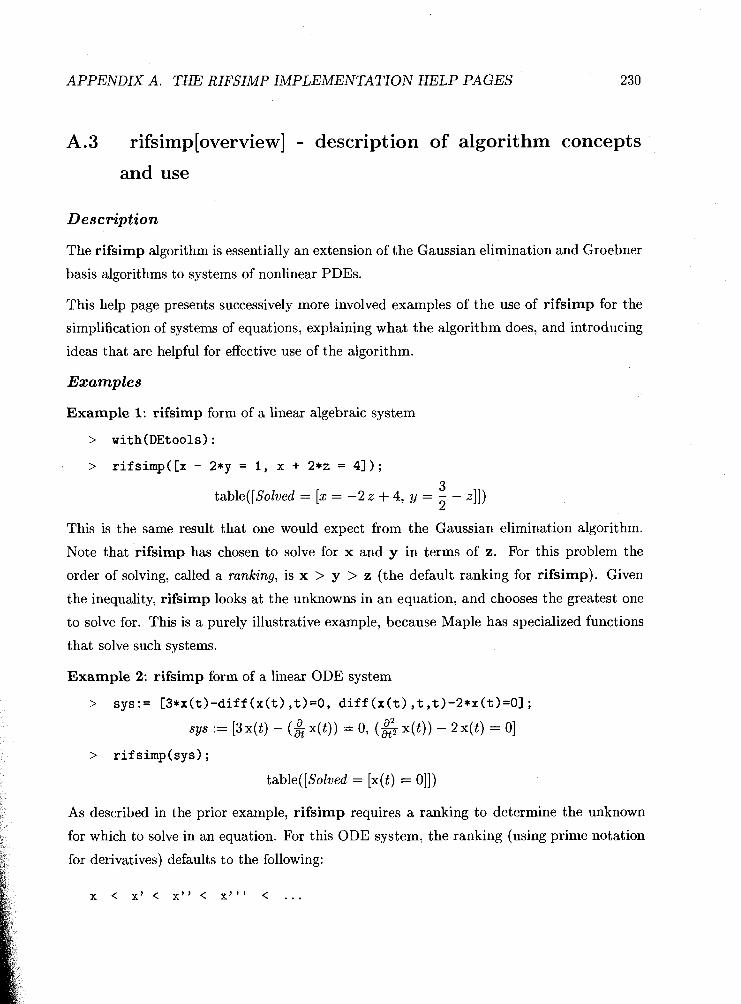
APPENDIX A. THE RIFSIMP IMPLEMENTATION HELP PAGES 230
A.3 rifsimp[overview] - description of algorithm concepts
and use
Description
The rifsimp algorithm is essentially an extension of the Gaussian elimination and Groebner
basis algorithms to systems of nonlinear PDEs.
This help page presents successively more involved examples of the use of rifsimp for the
simplification of systems of equations, explaining what the algorithm does, and introducing
ideas that are helpful for effective use of the algorithm.
Examples
Example 1: rifsimp form of a linear algebraic system
> with(DEtoo1s) :
> rifsimp([x - 2*y = 1, x + 2*2 = 41);
This is the same result that one would expect from the Gaussian elimination algorithm.
Note that rifsimp has chosen to solve for x and y in terms of z. For this problem the
order of solving, called a ranking, is x > y > z (the default ranking for rifsimp). Given
the inequality, rifsimp looks at the unknowns in an equation, and chooses the greatest one
to solve for. This is a purely illustrative example, because Maple has specialized functions
that solve such systems.
Example 2: rifsimp form of a linear ODE system
> sys:= [3*x(t)-diff (x(t) ,t)=O, diff (x(t) ,t,t)-2*x(t)=OI ;
a a2 sys := [3x(t) - (% x(t)) = 0, (= ~ ( t ) ) - 2x(t) = 01
> rifsimp(sys);
table([Solved = [x(t) = 011)
As described in the prior example, rifsimp requires a ranking to determine the unknown
for which to solve in an equation. For this ODE system, the ranking (using prime notation
for derivatives) defaults to the following:
X < x'< x" < x"' < . .

APPENDIX A. THE RIFSIMP IMPLEMENTATION HELP PAGES 231
So tho first equation is solved for x' giving x' = 3*x. The second equation is then differ-
entially simplified with respect to the first, and gives 3*x'-2*x = 0 after the first simplifi-
cation, and finally 7"x = 0 after the second. This equation is then solved for x, then back
substitution into the first equation gives 0 = 0.
For more general systems, rifsimp accounts for all of the derivative consequences of a system
in a systematic and rigorous way.
Example 3: rifsimp form of a nonlinear algebraic system > sys := [x-lO-2*~-5*y-2+y-4-y-3+1, 2*x-10-4*x-5*y-2+2*y-4+3*y-3-3,
> x-5-y-2+ye3-11 ;
sys := [x10 - 2 x 5 y 2 + y4 - Y 3 + 1 , 2x10 - 4 x 5 y 2 + 2 y 4 + 3 y 3 -3, x5 - y2+y3 -11
> rif simp(sys);
table([Constraint = [x5 - y2 = 0, -1 + y3 = 011)
The output was returned in the Constraint entries which means algebraic constraints as
opposed to differential constraints. For this system, rifsimp gives the Groebner basis form
of the algebraic system as output, as can be seen by running the Groebner package on the
same system (with the appropriate ranking).
In general, rifsimp on algebraic systems is closer to a factoring case splitting Groebner basis
(see rif simp [nonlinear], and Maple's Groebner package). rifsimp does not use Maple's
Groebner package, but instead its own, optimized for differential elimination.
Example 4: rifsimp form of a nonlinear ODE system > sys:= Cx(t)-3 + x(t) + 1 = O,diff(x(t),t,t)-3*diff(x(t),t)=O,
> diff (x(t) ,t,t,t)-2*diff (x(t) ,t)=01;
sys := [x(t)3 + ~ ( t ) + 1 = 0, (& X(t)) - 3 ( g x(t)) = 0, (6 x(t)) - 2 (g x(t)) = 01
> rif simp(sys) ;
table([Solved = [& x(t) = 01, Constraint = [ ~ ( t ) ~ + x(t) + 1 = 011)
Now the output is present in both the Solved and Constraint lists. The equation is present
in the constraint list because the leading indeterminate of the equation occurs nonlinearly
(for information on the leading indeterminate, please see rif simp Cranking]). Again, to

APPENDIX A. T H E R IFSIMP IMPLEMENTATION HELP PAGES 232
obtaill the answer, a ranking of the derivatives was required. The ranking used ranks "higher
derivatives in x ( t ) before lower derivatives". This is a fairly standard ranking called the
total degree ranking.
It is clear that the solution of the constraint equation gives x ( t ) = cons tan t , so from that
point of view, the equation in the derivative of x ( t ) is redundant, but it needs to be retained
for tho proper functioning of other algorithms, such as i n i t i a l d a t a , and r t ay lo r . The
additional equation in the Solved is a differential consequence of the Cons t ra in t , as can be
verifictl through differentiation. This redundant equation is called a spawn equation, as it is
a diffwential constraint spawned (through differentiation by t ) from the nonlinear equation.
Redundant equations can be removed with the clean or fullclean options as follows (see
r i f simp [options]):
> rifsimp(sys,clean=[spawnl);
table([Constraint = [ ~ ( t ) ~ + x(t) + 1 = 011)
> r i f simp(sys , fu l lc lean) ;
table([Constraint = [ ~ ( t ) ~ + x(t) + 1 = 011)
Example 5: rifsimp form of a linear PDE system > sys:= [diff (u(x,y) ,x,x) - y*diff (u(x,y) ,x) = 0 ,
> r i f simp(sys) ; a table([Solved = [z u(x, y) = 0 2 u(x, y) = 011) ' ay
In this example, rifsimp used the default ranking (where indices are used to denote differ-
ent iat ion)
This ranking satisfies the following properties:
1. It is preserved under differentiation (u < u[x] implies u[x] < u[xx]).
2. u is less than any derivative of u.
These two properties are crucial for the termination of the algorithm. Fortunately, the

APPENDIX A. THE RIFSIMP IMPLEMENTATION HELP PAGES 233
default rankings chosen by rifsimp obey these properties, so these do not have to be con-
siderctl. In general, many such ordering are possible, and methods for specifying them are
discussed in rif simp [ranking] and checkrank.
As an illustration, we will manually simplify the above system to rifsimp form. As the first
step, we solve each equation for its leading derivative (given the ranking described above).
This gives u[xx] = y u[x] and u[y] = 0. Alas, we do not have our final answer, but no
differential simplifications remain. How is this possible? Well, for PDE systems we have
one further consideration called integrability conditions.
After looking at our solved system for a time, we may realize that differentiation of the first
equation by y and differentiation of the second equation by x twice will give the derivative
u[xyy] on the left hand side of both equations. If the solution to the system is differentiable
to third order (an assumption implicitly made by rifsimp), we differentiate the equations
to thc described order and subtract, giving the new, nontrivial equation
Differential simplification of this equation with respect to the current system yields u[x] =
0, which is then used to simplify the system and give us the answer returned by rifsimp.
To summarize, for systems of linear PDEs, the rifsimp form of the system can be obtained
by the following heavily simplified algorithm, for a given input ranking <:
Rif simp-Linear (input : system, <)
neweqns := system
rif sys := empty
while neweqns not empty do
rifsys := rifsys union neweqns
rifsys := diff-gauss-elim(rifsys,rifsys,<)
neweqns := integrability-cond(rifsys)
neweqns := diff-gauss-elim(neweqns,rifsys,<)
end-while
return(rif sys)
end
Care must be taken in how the diff-gauss-elim routine operates on the solved rifsys.

APPENDIX A. THE RIFSIMP IMPLEMENTATION HELP PAGES
Example 6: rifsimp form of a nonlinear PDE system
This system is considered in the paper Reid et al., 1996 (see Rif) and is used as an example
in Rust, 1998. For the ranking u < u[x] < u[y] < u[xx] < u[xy] < U[YY] < ..., the
initial system consists of one leading linear PDE, u[xx]-u[xy] = 0 (with leading derivative
u[xx] ), and one leading nonlinear, PDE u[y] ̂ 2+u[y]-u = 0 (with leading derivative u[y]).
No linear elimination can be done in the single leading linear PDE, so the leading nonlinear
PDE is differentiated with respect to both independent variables to spawn the two leading
linear PDEs: (2 u[y]+l) u[xy]-u[x] = 0 and (2 u[y]+l) u [ ~ ~ ] - u [ ~ ] = 0 (for more
information on spawning, see r i f simp [nonlinear] ) . These are solved for their leading
derivatives, yielding u[xy] = u[x]/(2 u[y]+l) and u[yy] = u[y]/(2 u[y]+l), subject
to tho pivot or inequation condition 2 u[y]+l <> 0. Integrability conditions are then
taken across the leading linear PDE and simplified subject to the system, yielding one
more PDE: u[x] u[y]-u[x] -2 = 0. When this equation is spawned, the resulting equations
vanish to zero upon reduction by the current system, so the algorithm then terminates. In
summary, constraints are treated algebraically, and the leading linear equations are treated
differentially. The system is then viewed modulo the constraint equations, using the concept
of a relative basis, rigorously described in the thesis of Rust (see references on the Rif help
page). > sys:= [diff (u(x,y) ,x ,x) - d i f f (u(x,y) ,x ,y) = 0 ,
> d i f f (u(x,y) ,y )^2 + d i f f (u(x,y) ,y) - u(x,y) = 01 ; a2 a2
SYS := [(=u(x, Y)) - (= u(x, Y)) = 07 (&u(x, Y H 2 + (& u(x, 9)) - u(x, Y) = 01
> r i f simp(sys) ;
Example 7: rifsimp form of a nonlinear PDE system with cases

APPENDIX A. THE RIFSIMP IMPLEMENTATION HELP PAGES 235
This problem arises from the determination of Lie symmetry groups for different values of
a , b for the ODE:
> ODE := diff(y(x),x,x)-2*a-2*y(x)^3+2*a*b*x*y(x)-b;
ODE := ( f$ y(x)) - 2 a2 y(x)3 + 2 a bx y(x) - b
The Lie symmetry determining equation can be obtained through use of the DEtools Cgensysl
function as follows:
> sys := { g e n s y s ( O ~ ~ , [xi , e ta ] (x ,y) )} ;
sys := {-q(x, y ) (6a2y2 - 2 a b x ) - 2 ( 2 a 2 y 3 - 2 a b x y + b ) ( & [ ( x , y))
+ P a 2 y3 - 2 . b ~ ~ + b) (& d x , Y)) + ~ F ( x , YWY + (& d x , Y)), a2 (& d x , Y)) - 2 (& tb, Y))? t (x , Y),
-3 @a2 y3 - 2 a b x y + b) (& t ( x , Y)) + 2 (& 1)(5, Y)) - (f$ [(I, Y))}
When viewed as a system in xi and e ta , it is a linear system, but if we are also considering
a ,b to be unknowns, the system becomes effectively nonlinear. Now what we want to
accomplish is to find the equations for the symmetry generators for all values of a,b. We
can do this by allowing rifsimp to perform case splitting on the system using the casesplit
option (see rif simp [cases] for more detail).
> ans:=rifsimp(sys,casesplit);

APPENDIX A. THE RIFSIMP IMPLEMENTATION HELP PAGES
ans := table([l = table([Solved = [q(x, y) = 0, [(x, y) = 01,
= [[a # 0, &(x, Y)l, [b # 0, q(x, Y) l l , Pivots = [a # 0, b # O]]),
a a ~ ( x , Y) a ~ ( 2 , Y) 2 = table([Solved = [& q(x, y) = 0, ((x, y) = --, q(x, y) = -, Y Y
g F F(x, 9) = 0, a = 01,
Gme = [[a = 0 ' ay t (x, Y)111>,
casecount = 31)
The structure of the output of rifsimp has changed form into a recursive table for multiple
cases. The returned table has a casecount entry, and individual rifsimp answers for each
case indexed by the numbers 1,2,3. For the three cases, the form of the Solved equations
for xi,eta is different. This indicates that for different values of a ,b the structure of the Lie
symmetry group is different, and provides the systems that must be satisfied for each group.
This case splitting also covers all possible values of a,b, so it fully describes the dependence
of the determining system on these values, and no other systems for other values of a,b
exist.
The structure of the case tree can be observed in a plot using caseplot.
> caseplot (am) ;

APPENDIX A. THE RIFSIMP IMPLEMENTATION HELP PAGES
A.4 rifsimp[output] - description of algorithm output
Description The output of the rifsimp command is a table. A number of possible
table formats (or entries) may or may not be present as they depend on specific options.
The format changes from a table containing the simplified system to a nested table when
casesplit is activated.
Single Case
Solved
Pivots
Case
This entry gives all equations that have been solved in
terms of their leading indeterminate.
This entry gives all inequations (equations of the form
expression <> 0) that hold for this case. These may be part of the input system, or decisions made by the program during
the calculation (see rifsimp[casesl for information on
pivots introduced by the algorithm).
This entry describes what assumptions were made to arrive
at this simplified system (see rifsimpCcases].)
Constraint This table contains all equations that are nonlinear in
their leading indeterminate. The equations in this list
form a Groebner basis and can be viewed as purely algebraic
because any differential consequences that result from these
equations are already taken care of through spawning
(see rif simp [nonlinear] . If the initial option has been specified, then these
equations are isolated for the highest power of their
leading derivatives, otherwise they are in the form expr=O.
DiffConstraint This table entry contains all equations that are nonlinear
in their leading indeterminate, but either are not in
Groebner basis form or have differential consequences that

APPENDIX A. THE RIFSIMP IMPLEMENTATION HELP PAGES
status
are not accounted for (see spoly and spawn
in rif simp [nonlinear] ) . Whenever equations appear in this entry, the system is in
incomplete form and must be examined with care.
This table entry contains all equations that rifsimp did
not attempt to solve (see unsolved in rifsimpCadv-options]).
Whenever equations appear in this entry, the system is in
incomplete form and must be examined with care.
This table entry contains all equations that have not yet
been examined (i.e. Unclassified). This entry is only
present when looking at partial calculations using rifread,
or when a computation is halted by mindim.
If this entry is present, then the output system is missing
due to either a restriction or an error. The message in
this entry indicates what the restriction or error is.
dimension This entry is only present when the mindim option is used
(see rifsimp[casesl), or for maxdimsystems.
For the case where a single constraint is in effect (such
as through use of the option mindim=8), the right-hand side
is a single number (the dimension for the case). For
multiple constraints, it is a list of dimension counts,
one for each constraint in the mindim specification.
Here are examples of status messages:
"system is inconsistent" No solution exists for this system
"object too large" Expression swell has exceed Maple's
ability to calculate

APPENDIX A. THE RIFSIMP IMPLEMENTATION HELP PAGES 239
"time expired" Input time l i m i t has been exceeded (see
c t l , s t l and it1 i n rifsimpCoptions1)
" f ree count f e l l below mindim" Free parameters have f a l l e n below the
minimum (see mindim i n r i f simp Cadv-options] )
Of tho above, only the "object too large" message actually indicates an error.
To surnmarize, if the input system is fully linear in all indeterminates (including unknown
constants), then only the Solved entry will be present. If the system is (and remains) linear
in its leading indeterminates throughout the calculation, but has indeterminate expressions
in tho leading coefficients, then Solved, Pivots, and Case will be present. If equations that
are nonlinear in their leading indeterminates result during a calculation, then Constraint
will also be present. If the s ta tus entry is present, then not all information for the case will
be given.
If mindim is used, then the dimension entry will be set to the dimension of the linear part
of the system for the case when s t a tu s is not set, and an upper bound for the dimension of
the case if the count fell below the minimum dimension requirement.
Multiple Cases
For multiple cases (using the casesplit option), numbered entries appear in the output
table, each of which is itself a table of the form described above.
For example, if a calculation resulted in 10 cases, the output table would have entries
'1= ...',..., 'lo=...', where each of these entries is itself a table that contains Solved, Pivots,
Case, or other entries from the single case description.
In addition to the numbered tables is the entry casecount, which gives a count of the
number of cases explored. Cases that rejected for reasons other than inconsistency will have
the Case entry assigned, in addition to the s t a tu s entry. Inconsistent cases, for multiple
case solutions, are removed automatically.
So what is the difference between Pivots and Case?
The Pivots entry contains the inequations for the given case in simplified form with re-
spect to the output system. The Case entry is a list with elements of the form [as-
sumption,leading derivative] or [assumption,leading derivative,"false split"]. It

APPENDIX A. THE RIFSIMP IMPLEMENTATION HELP PAGES 240
describes the actual decision made for the case split in unsimplified form (i.e. as it was
encouutered in the algorithm). The assumption will be of the form expr<>O or expr=O,
where expr depends on the dependent variables, derivatives and/or constants of the prob-
lem. The leading derivative is the indeterminate the algorithm was isolating that required
the assumption. If the third "false split" entry is present, then it was later discovered that
one branch of the split is entirely inconsistent, so the actual splitting was a false splitting, as
the displayed assumption is always true with respect to the rest of the system. For example,
if the algorithm were to split on an equation of the form a*diff(f(y),y)+f(y)=O, the Case
entrics that correspond to this case split are [a< >O,diff(f(y),y)], and [a=O,diff(f(y) ,y)].
If it was found later in the algorithm that a=O leads to a contradiction, then the Case
entry would be given by [a<>O,diff(f(y),y)," false split"].
Note that when faclimit or factoring are used (of which factoring is turned on by
default), it is possible to introduce a splitting that does not isolate a specific derivative.
Wheli this occurs, the case entry will be of the form [assumption,"faclimit"] or [as-
sumption," factor"].
Occasionally both the Case and Pivots entries contain the same information, but it should
be understood that they represent different things.
Impor tan t
As discussed above, some options have the effect of preventing rifsimp from fully simplifying
the system. Whenever DiffConstraint or UnSolve entries are present in the output,
some parts of the algorithm have been disabled by options, and the resulting cases must be
manually examined for consistency and completeness.
Examples
> with(DEtoo1s) :
As a first example, we take the overdetermined system of two equations in one dependent
variable f(x), and two constants a and b.
> sys1:=[a*diff(f(x),x,x)-f(x),b*diff(f(x),x)-f(x~];
sysl := [a (& f(x)) - f(x), b (& f(x)) - f(x)]
Call rifsimp for a single case only (the default).
> ansl:=rifsimp(sysl);

APPENDIX A. THE RIFSIMP IMPLEMENTATION HELP PAGES
ansl := table([Case = [[a # 0, & f(x)], [b # 0, &f(x)], [b2 - a # 0, f(x)]],
Solved = [f(x) = 01,
Pivots = [a # 0, b # 0, b2 - a # 0]
I ) We scc that under the given assumptions for the form of a and b (from Pivots), the only
solution is given as f(x)=O (from Solved). Now, run the system in multiple case mode
using casesplit.
anslm := table([l=table([Cose = [[a # 0, &f(x)], [b # 0, &f(x)], [b2 - a # 0, f(x)]],
Solved = [f(x) = 01,
Pivots = [a # 0, b # 0, b2 - a # 0]
I), 2 = table([Case = [[a # 0, & f(x)], [b # 0, & f(x)], [b2 - a = 0, f(s)]],
f ( 4 Solved = [& f(z) = -, a = b2], b
Pivots = [b # 01
I), 4 = table([Cose = [[a = 0, & f(s)]], Solved = [f(z) = 0, a = O]]),
casecount = 4 I )
We see that we have four cases:
All cases except 2 have f(x)=O.
Looking at case 2 in detail, we see that under the constraint a = b-2 (from Solved) and
b <> 0 from Pivots, the solution to the system will be given by the remaining ODE in
f(x) (in Solved). Note here that the constraint on the constants a and b, together with
the assumption b <> 0, imply that a <> 0, so this constraint is not present in the Pivots
entry due to simplification. It is still present in the Case entry because Case describes
the decisions made in the algorithm, not their simplified result. Also, case 4 has no Pivots
entry. This is because no assumptions of the form expression <> 0 were used for this

APPENDIX A. THE RIFSIMP IMPLEMENTATION HELP PAGES
case.
One could look at the caseplot with the command:
> caseplot (anslm) ;
As a final demonstration involving this system, suppose that we are only interested in
nontrivial cases where f(x) is not identically zero. We can simply include this assumption
in thc input system, and rifsimp will take it into account.
> ansla:=rif simp( [op(sysl) ,f (x)<>Ol ,casesplit) ;
onsl a := table([Case = [[a # 0, & f(x), "false split"], [b # 0, & f(x), "false split"]],
a f(4 2 Solved = [= f(x) = -, a = b 1, b
Pivots = [f(x) # 01 I )
We see that the answer is returned in a single case with two false split Case entries. This
means the computation discovered that the a = O and b=O cases lead to contradictions, so
the entries in the Case list are labelled as false splits, and the alternatives for the binary
case splittings (cases with a = O or b = O ) are not present.
For the next example, we have a simple inconsistent system:
> sys2:=[diff(u(x),x,x)+diff(u(x),x)~2-1,diff(u~x~,x,x~+1~;
sys2 := [(& 4 x 1 ) + (& u(xN2 - 1, (& 4x1) + 11 > rifsimp(sys2) ;
table([status = "system is inconsistent"])
So there is no solution u(x) to the above system of equations.
The next example demonstrates the UnSolve list, while also warning about leaving inde-
terminates in unsolved form.
> sys3:=[diff(f(x),x)*(diff(g(x),x)-g(x))+f(x)~2,diff(g(x),x~-g~x~~;
sys3 := [(& f(x)) ((& d x ) ) - g(x)) + w2, (& ~ ( 4 ) - g(41
So we run rifsimp, but only solve for f(x), leaving g(x) in unsolved form. Unfortunately,
the resulting system is inconsistent, but this is not recognized because equations containing
only g(x) are left unsolved. As discussed earlier in the page, these equations come out in
the UnSolve list.

APPENDIX A. THE RIFSIMP IMPLEMENTATION HELP PAGES
> rif simp(sys3, [f 1 ,unsolved) ;
fM2 table([Case = [[%I # 0, &f(x)]], Solved = [g f(x) = --I, Pivots = [%1 # 01, %1
UnSolve = [0 = %1]
I ) %I := (& g(x)) - g(x)
When equations are present in the UnSolve list, they must be manually examined.
Here is a nonlinear example.
> sys4 : = [dif f (f (x) , x ,x) +f (x) , di f f (f (x) ,x) -2-f (x) -21 ;
sys4 := [(& f b ) ) + fb), ( 6 f(x)I2 - f ( ~ ) ~ l By default rifsimp spawns the nonlinear equation to obtain a leading linear equation, and
performs any required simplifications. The end result gives the following output:
> rifsimp(sys4,casesplit);
table([Case = [[f(x) = 0, & f(x), "false split"]], Solved = [f(x) = 011)
We have only one consistent case. Attempting to perform this calculation with the
spawn=false option gives the following:
So it is clear that by disabling spawning, the system is not in fully simplified form (as indi-
cated by the presence of the DiffConstraint entry), and we do not obtain full information
about the system.

APPENDIX A. THE RIFSIMP IMPLEMENTATION HELP PAGES
A.5 rifsimp[options] - common options
Description
The rifsimp options are given after the input system, and optionally the vars. The following
are tho most commonly used options:
vars
This is the optional second argument to rifsimp. It indicates which indeterminates are to be
solved for. By default rifsimp attempts to solve for all dependent variables with the same
differctntial order and differentiations with equal precedence, breaking ties alphabetically.
rifsimp solves for constants when only constants remain in an equation.
The sctlection of the solving indeterminate (called the leading indeterminate) of an equation
is performed based on the ranking imposed on the system. This argument can be used
in nested list form to modify the indeterminates to solve for. For example, if f(x), g(x) ,
and h(x) were the dependent variables of a problem, and we wanted to isolate all of these
with cqual precedence, we could specify vars as [f,g,h]. If instead we wanted to eliminate
f(x) from as much of the system as possible, we could specify [[f],[g,h]] instead, which
tells rifsimp to solve for f(x) and its derivatives with higher precedence than g(x) , h (x)
and any of their derivatives, regardless of the differential order of f(x). Under this nested
list ranking, and equation of the form g"' f-g" h"=O would be solved for f giving f=gV
h" /g" '. See rif simp [ranking] and checkrank for more detail.
indep=[indl,ind2,.. .]
This option specifies the names of the unknowns to be treated as independent variables.
By default, only those unknowns given in the dependency list of all unknown functions
in the input system are considered to be independent variables. All other unknowns are
considered constants. Treating an independent variable as though it were a constant will
result in an incomplete answer, so you must use this option when required (see examples
below). Please note that rifsimp always views unknowns present in a dependency list of
an unknown function as independent variables, even when not specified by this option.
The order in which the independent variables are specified in this option affects the selec-
tion of the leading indeterminate (the indeterminate to be solved for) in an equation. See
rif simp [ranking] and checkrank for details.

APPENDIX A. THE RIFSIMP IMPLEMENTATION HELP PAGES
This option specifies a list of parameters or functions that should be treated as arbitrary.
Any special cases where these parameters or functions take on specific values are rejected as
inconsistent cases. Note: This means that no relations purely in the arbitrary parameters
or fu~~ctions can be present in the input system (with the sole exception of dependency
relatcd equations such as diff(f(x,y),y)=O). If a constraint is required for one of these
unknowns, then it is no longer truly arbitrary, but rather restricted, so a t least one of the
unknowns in the constraint must be a solving variable.
This option generalizes the concept of a f i e l d of constants as used in the d i f f a l g pack-
age to functions of the independent variables. It is most useful when only generic results
are needed, but it may be the case that the result is invalid for specific values of these
parameters (for example, if a was a parameter, and it occurred as a denominator, then the
solution is only valid for a< >0) .
casesplit
This option indicates that the program should explore all cases. A case split is most often
introduced when, among the remaining unsolved equations, there is an equation that is linear
in its highest ranked indeterminate (called the leading indeterminate, see r i f simp [ranking]
or checkrank), and the coefficient of that indeterminate (called the pivot) may or may not
be zero (see rif simp [cases]).
I Isolation of the leading indeterminate in this equation introduces a case split - namely the
two possibilities, pivot <> 0 and pivot = 0. The more generic case, pivot <> 0, is
explored first. Once that case (possibly containing further case splits) is completed, the
case with pivot = 0 is explored. This results in a case tree, which can be represented
graphically (see caseplot) .
In addition to producing multiple cases, this option changes the output of rifsimp. For
more detail, see r i f simp [output].
gens01
This option indicates that the program should explore all cases that have the possibility of
leading to the most general solution of the problem. Occasionally it is possible for r i fs imp
to compute only the case corresponding to the general solution of the ODE/PDE system.

APPENDIX A. THE RIFSIMP IMPLEMENTATION HELP PAGES 246
When this option is given, and this occurs, rifsimp will return the single case corresponding
to the general solution. When it is not possible for rifsimp to detect where in the case tree
the gcneral solution is, then multiple cases are returned, one or more of which correspond
to tha general solution of the ODE/PDE system, and others may correspond to singular
solutions. For some particularly difficult problems, it is possible that the entire case tree is
returned. Note: this option cannot be used with the casesplit,casecount, pivsub, and
mindim options.
This option imposes a limit on the amount of time (in CPU seconds) that would be required
to corripute each case from scratch (i.e. using the extended option casesplit=[ ...I described
in r i f simp [adv-options1 ). It is clear that this option may count computation time more
than once, as the time prior to a case split is counted for each case after the split. This
bounds the total time consumed to be no greater than the imposed limit times the number
of casos obtained (and most often, significantly less as per the prior comment). For highly
nonli~iear systems, it may be impossible to obtain all cases in a reasonable amount of time.
Use of this option allows the simpler cases to be computed, and the more expensive cases
to be deferred. Note: there are two other time limit related options, st1 and it l , and these
are discussed in the r i f simp [advnptionsl page.
clean= [cleaning criteria]
This option is a fine-tuning control over the system(s) output by rifsimp. There are three I
types of cleaning that the algorithm can perform:
Pivots: These are the inequations resulting from case splitting in the system (or present
on input). As an example, consider the pivot diff(f(x),x)<>O. This pivot clearly implies
that f(x)<>O, so on completion, the pivot f(x)<>O is considered to be redundant. There
are three options for specification of pivot cleaning:
nopiv perform no cleaning, r e tu rn ing all pivots obtained
i n t he course of t h e computation.
piv perform cleaning of obvious redundant p ivots ( i . e .
those t h a t can be de tec ted by inspec t ion of t he
pivots l i s t on output .
f u l l p iv perform thorough cleaning of p i v o t s , including

APPENDIX A. THE RIFSIMP IMPLEMENTATION HELP PAGES
removal of p ivots t h a t a re redundant only f o r
so lu t ions of t he output case/system.
No te that the fullpiv criteria may remove pivots that would require a great deal of compu-
tation to recover. For example, consider the simple case described earlier for diff(f(x),x) <> 0. If later in the algorithm, diff(f(x),x) was reduced, and looked nothing like the origi-
nal pivot, on completion f(x)<>O, which is a consequence of the original pivot, would be
removed.
One-Term Equations: These are simply equations of the form derivative=O. These are
retair~cd in the course of the computation (for efficiency) even when they reduce modulo one
of thc other equations of the system. These equations can be quite helpful in attempting
to intctgrate of the results of rifsimp. The one te rm criteria indicates that the redundant
one-term equations should be removed, while nooneterm indicates that they should be
retained.
Spawn: The spawning process is only used with nonlinear equations in rifsimp, and results
in equations that are derivatives of any nonlinear equations in the output. These spawned
equations are necessary for the proper running of i n i t i a l d a t a and r t ay lo r . The following
options specify spawned equation cleaning:
nospawn do not remove any redundant spawned equations
spawn remove any redundant spawned equations t h a t a r e not
i n solved form.
fullspawn remove a l l redundant spawned equations.
By default, the clean settings are [piv,oneterm,nospawn] .
fullclean
This is a shortcut specification for the clean options for rifsimp (see above). This corre-
sponds to the specification clean= [fullpiv,oneterm,fulIspawn] .
Examples
> with(DEtoo1s):
This example highlights the difference between treating the unknown y as a constant and
treating it as an independent variable; by default, the code assumes that y is a constant.

APPENDIX A. THE RIFSIMP IMPLEMENTATION HELP PAGES 248
> sysl :=Cy*f (x)+g(x)l ;
sysl := [y f(x) + g(x)]
> rif simp(sys1) ;
g ( 4 table([Solved = [f(x) = --I, Pivots = [y # 01, Case = [[y # 0, f(x)]]]) Y
Specification of y as an independent variable gives the following.
> rifsimp(sysl,indep=[x,y]) ;
table([Solved = [f(x) = 0, g(x) = 011)
This next example demonstrates the use of the casesplit option. We consider the Lie-
symnletry determining system for the following ODE:
> ODE:=diff (y(x) ,x,x)+(2*y(x)+f (x) )*diff (y(x) ,x)+dif f (f (XI ,x)*y(x) ;
ODE := ($2 ~ ( 4 ) + ( ~ Y ( x ) + f ( 4 ) (& ~ ( 4 ) + (aa; f ( 4 ) ~ ( 4
The Lie symmetries are given as the solution of the following system of determining PDEs
(as generated using DEtools Codepde]):
> sys:=Ccoeffs(expand(odepde(ODE, Cxi(x,y) ,eta(x,y)l, y(x) 1) ,-yl)] ;
And we see that the given ODE has no point symmetries for general f(x).
We may want to know if there are particular forms of f(x) for which point symmetries exist
(this is called a classification problem). Running rifsimp with casesplit: > ans :=rif simp(sys, Cxi,etal ,casesplit) :
> ans C' casecount 'I ;

APPENDIX A. T H E RIFSIMP IMPLEMENTATION HELP PAGES
so we see there are cases.
We could use the caseplot command to give a pictorial view of the case tree with the
following command.
> caseplot (am) ;
Looking at case 3 in detail:
> copy (ans C31) ;
Pivots = [& f(x) # 01,
Case = 1[-3 (& f(x)) (& f(x)) + 2 (& f(x)) y + (& f(x)) f(x) + 2 (& f ( ~ ) ) ~ y
- 2 (& f(xH2 f(5) + fW2 (& f(x)) + 2 f(x) (& fb)) Y = 0, t (5, y)],
rC f(x) z 0, 6 ~ ( X ) I I
I ) so we see we have a 2 parameter Lie group for the specific form of f(x) given by:

APPENDIX A. THE RIFSIMP IMPLEMENTATION HELP PAGES
A. 6 rifsimp [adv-opt ions] - advanced opt ions
Description
The rifsimp options are given after the input system, and optionally the vars.
The following are the advanced options:
Store the system after each iteration in a file called name.m (default is RifSt0rage.m).
Note: when multiple cases are being examined, only the latest iteration of the current case
is available. Iterations can be observed by setting infolevel[rifsimp] to 2 or greater. This
file call be read using the r i f read command.
Store the system iterations separately in a file called name-cs-i.m, where cs is the current
case number, and i is the current iteration number (default is RifStorage-cs-i.m). This file
can bc read using the r i f read command.
ezcriteria= [quantity, size ratio]
The ezcriteria option allows control over how quickly equations are chosen for solving.
quantity is a factor that adjusts the number of equations selected, while the size ratio tells
rifsimp how large a difference in size can exist between the smallest and largest equations
chosen in a single iteration. I
The number of equations selected in a single iteration is based upon the number that have
already been solved. So if we have no equations solved for their leading derivative, then the
algorithm will select at most 10 new equations, whereas if there are 200 equations already in
solved form, only one new equation will be selected. The option works this way to control
how much work is done in each iteration, since adding one equation when there are no
equations in solved form requires no checking of compatibility (integrability) conditions,
while adding one equation to the 100 already in solved form may require checking of 100
compatibility conditions.
The size ratio enforces a maximum difference in size between the smallest and largest equa-
tions chosen in an iteration. If the size ratio was set to 2 (the default), and the three
equations remaining to be solved have sizes of 100, 190, 400, 500, then even if the number

APPENDIX A. THE RIFSIMP IMPLEMENTATION HELP PAGES 251
to bc selected based on the quantity was more than 2, only the first two equations will be
selected, as equations 3 and 4 are more than double the size of equation 1.
Primary uses of this option are for the ultra-conservative setting of [1,0.9], and the setting
of [infinity,infinity] at the other extreme.
This option indicates that the first n equations or expressions in the input system are to be
placed into solved form immediately. If an inequation is present in the first n equations, it
is not counted as one of the first n equations. This option is only available when the system
has boen specified in list form.
unsolved
This tells Maple not to solve for any dependent variables or constants not explicitly men-
tioned in vars. It should only be used used when rifsimp is being used as a preprocessor.
It is inadvisable to use this option with nonlinear equations, as it can result in infinite loops,
may prevent inconsistent cases from being recognized, and does not result in a disjoint set
of cases. This option cannot be used with the arbitrary option (see r i f simp [options]).
This option imposes a limit on the amount of time (in CPU seconds) spent on the calculation
since the last case split occurred. Use of this option allows the simpler calculations to be
performed, and the more expensive calculations to be deferred. Note, this option is quite
different from ctl, as it does not come into effect until the first splitting starts, and only
bounds time between splittings. This has the effect of screening out cases that are not
making progress quickly enough.
This option imposes a limit on the amount of time (in CPU seconds) spent on any single
iteration. An iteration consists of selecting one or more equations to isolate, adding them to
the solved list, simplifying the existing system with respect to the new simplified equations,
and then considering all consequences that the new equations have with respect to the
already-solved equations in the system. Iterations in a calculation can be viewed by setting
the rifsimp infolevel to 2 or greater.
ranking=[[ind weights 1, dep weights 11, [ind weights 2, dep weights 21, ...I

APPENDIX A. THE RIFSIMP IMPLEMENTATION HELP PAGES 252
This gives the linear ordering used to determine the relative weights of the dependent
variable derivatives. See rif simp [ranking] for more information.
ca~esplit=['<>~,'=','< >'I
This option turns on case splitting and also gives the start of the tree which will be examined.
See rif simp [cases] for further details.
mindim= ... This option is used to limit the cases being examined based on the solution space dimension
of the linear part of the system. The simple specification is given as mindim='n'. If vars
is specified as a simple list, this gives the minimum of n free 0-dimensional parameters in
the vars dependent variables. If vars contains lists, it is specified as part of a ranking (see
rifsimpCrankingl), and only the first element of vars is used to compute the dimension.
Once the condition fails, the current case is discarded.
NOTE: mindim only looks at the linear part of the current system, so if nonlinear con-
straints are present, the actual dimension may be lower than the dimension reported.
It is possible to give more detailed and/or multiple specifications for a calculation. Please
see rif simp [casesl for the more advanced usage, and additional information.
pivselect =choice
This option gives some control over how rifsimp performs case splitting. More information
can be found in rif simp [cases].
nopiv= [varl, . . .] This option gives a list of all variables and constants which cannot be present in pivots.
This is most useful for quasi-linear systems for which the linearity of the resulting system
is of greatest importance. This may also have the effect of reducing the size of the case
tree in these systems. The unsolved equations are then treated as fully nonlinear (see
rif s imp [nonlinear] ) .
faclimit =n
Typically the pivot chosen is the coefficient of the leading indeterminate in the equation.
In the event that the leading indeterminate is itself a factor of the equation, and this same
leading indeterminate factor occurs in n or more equations, then it is chosen as the pivot

APPENDIX A. THE RIFSIMP IMPLEMENTATION HELP PAGES
rather than the coefficient. See rif simp [cases] for more information.
This is most useful for Lie determining systems having many inconsistent cases, since many
equations of this form typically occur during the calculation. The answer may be obtained
without this option, but it has the beneficial effect of reducing the number of cases.
This option is used to control introduction of pivots that are not necessarily the leading
coefficient of an equation. Basically, if no leading linear equations remain in the unsolved
equations, then depending on the value of this parameter, if the unsolved equations can be
factored, a split will be performed on that factor. If desc=none, then this is disabled; if
desc=nolead, then factors may only be chosen if they do not contain the leading derivative
(this is the default); if desc=all then any factor can be split on. See rif s imp [cases] for
more detail.
Note that use of factoring=none can result in non-termination for some nonlinear prob-
lems.
checkempty
This option tells rifsimp to try to eliminate any empty cases in the computed result(s).
These can only occur when both pivots and nonlinear equations are present in the result,
and is quite uncommon. This is not done by default (See rif simp [nonlinear] for details).
grobonly
This option tells rifsimp to only use Groebner basis simplification for the leading nonlinear
equations instead of the more efficient method described in rif simp [nonlinear] .
initial
This option tells rifsimp to isolate the highest power of the leading derivative of each
equation in the Constraint list, performing further case splitting on the coefficient if re-
quired. This causes the output case structure to more closely resemble that of diffalg,
and changes the form of the equations in Constraint. This option is enabled by default
unless grobonly is specified (see rif simp [output]). For more information on this option,
please see rif simp [cases].

APPENDIX A. THE RIFSIMP IMPLEMENTATION HELP PAGES
This option controls the ranking for algebraic Groebner basis sub-computations.
See rif simp [nonlinear] for details.
This option indicates whether to generate S-polynomials during the Groebner basis algo-
rithm (default is true). Setting spoly=false has some risk associated with it, and if non-
linear equations are present in the output, then it is possible that not all consequences of
these equations have been obtained (hence they are placed in the DiffConstraint list rather
than the Constraint list). If an orderly ranking is used (see rif simp Cranking1 , and spawn
is set to true, then only algebraic simplifications remain, but these may still result in an
incorlsistent system when considered with the Pivot equations.
This option indicates whether to perform a differential spawn of nonlinear equations (default
is true). Setting this to false makes the program ignore any differential consequences of
the polynomially nonlinear equations. This is only useful if rifsimp is being used as a
single step of a different calculation, since an incomplete answer will be obtained. See
rif simp [nonlinear].
For a description and examples of the above options, please see the specific pages describing
those opt ions:
ranking See rifsimp,ranking
casesplit, mindim, pivselect, nopiv, See rifsimp,cases
faclimit, pivsub, factoring, initial " grobonly, grob-rank, spoly, spawn, See rifsimp,nonlinear3
checkempty #I

APPENDIX A. THE RIFSIMP IMPLEMENTATION HELP PAGES 255
A.7 rifsimp[ranking] - understanding rankings and related
concepts
Description
What is a ranking?
A ranking is essentially an ordering of all indeterminates in a system. To introduce rankings,
we must first introduce some related concepts.
Dependent variable
This term describes any unknown function that is present in the input system. As an
example, consider a system involving f(x,y) and its derivatives, g(x,y) and its derivatives,
and exp(x). In a calculation, you may want to view f(x,y) as the solving variable, and
g ( x , ~ ) as a parameter. Even in this case, these are both considered to be dependent
variables. Because exp(x) is a known function, it is not considered t o be a dependent
variable.
Independent variable
For a problem containing f(x,y) and its derivatives, g(x,y) and its derivatives, and exp(x) ,
x and y are the independent variables.
Constants
Any unknown not having a dependency, and not occurring in a dependency, is considered
to be a constant. This is true even if it appears in a known function. For example, in the
equation a*f(x,y)+sin(c)*g(x,y), both a and c are considered to be constants.
Note: The distinction between independent variables and constants is vital, since mistaking
one for the other will not give a valid result for a system. For information on the specification
of independent variables, please see rif simp [options].
Indeterminate
An indeterminate can be any constant, dependent variable, or derivative of a dependent
variable. This does not include any known functions or independent variables. This is
exactly the group of items that a ranking is defined for.

APPENDIX A. THE RIFSIMP IMPLEMENTATION HELP PAGES
Ranking
A ranking is a strict ordering of all indeterminates appearing in a system in the course of a
calculation. Note that it is necessary to rank more than just the indeterminates appearing
in the initial system, because higher derivatives may appear in the course of the algorithm.
Leading indeterminate
The lcading indeterminate of an equation is defined as the indeterminate in that equation
that is of the highest rank (maximal with respect to the ranking).
The concept of a leading indeterminate is important for understanding how the rifsimp
algorithm works, because any equation in which the leading indeterminate appears linearly
is solvcd with respect to that indeterminate.
Properties of a ranking
Rankings have a number of properties, some of which are required for the proper performance
and termination of the algorithm, others of which may be helpful in tackling specific systems.
In any of the descriptions below, v l and v2 are indeterminates that may depend on some
of xl , x2, x3, ... Preservation of ranking under differentiation
Given a ranking v l > v2, this ranking also holds after equal differentiation of both v l
and v2 with respect to any independent variable, for all vl , v2 where v l and v2 are
indeterminates.
Note: You must restrict yourself to non-vanishing indeterminates (for example, for h(x)
> g(x,y), differentiation with respect to y makes h(x) vanish, so the rule does not apply).
This property is required for the proper running of rifsimp. Once an equation is solved
for the leading indeterminate, any differentiation of that equation (assuming that the lead-
ing indeterminate does not vanish) is also in solved form with respect to its new leading
indeterminate (the derivative of the prior leading indeterminate).
Positive ranking
Given a ranking >, it must be true that diff(v1,xl) > v l for all indeterminates v l and all
independent variables x l , as long as diff(v1,xl) is nonzero.

APPENDIX A. THE RIFSIMP IMPLEMENTATION HELP PAGES 257
This property is required for the proper running of rifsimp, because it prevents any infinite
chain of differential substitutions from occurring.
As an example, consider the solved form of the equation u[t]-u[tt] = 0 under a non-positive
ranking u[t] = u[tt]. Differential elimination of the derivative u[xt] with respect to this
equation will give u[xtt], then ~ [ x t t t ] , then ~ [ x t t t t ] , and so on. It will never terminate.
Total-degree ranking
Let dord() give the total differential order of an indeterminate with respect to all inde-
pendmt variables. Then for v l and v2 derivatives of the same dependent variable, given a
ranking >, then dord(v1) larger than dord(v2) implies v l > v2.
For rifsimp to run correctly, a ranking does not have to be total degree. In some cases
this does allow rifsimp to run faster, however. For those familiar with Groebner basis
theory, a total degree ranking is similar to a total degree Groebner basis ordering, because
calculations usually terminate more quickly than they would with a lexicographic ordering.
Orderly ranking
A ranking is said to be orderly if, for any indeterminate, no infinite sets of indeterminates
that are lower in the ordering exist.
As an example of a ranking that is not orderly, we consider a ranking of f(x), g(x), and
of all derivatives. If we choose to solve a system using rifsimp for f(x) in terms of g(x)
(by specification of only f(x) in the solving variables), then this is not an orderly ranking,
because g(x) and all of its derivatives are of lower rank than f(x) and any of its derivatives.
For rifsimp to run correctly, using the defaults for nonlinear equations, a ranking is not
required to be orderly (see r if s imp [nonlinear] .)
T h e Default ranking
The rifsimp default ranking is an orderly, total-degree ranking that is both positive and
preserved under differentiation. Note that if the solving variables are specified, we may
no longer be using the default ranking (since specification of solving variables alters the
ranking. See "Specification of a ranking" below.
On input, rifsimp assumes that all dependent variables present in the input system are
solving variables, and that all constants are to be viewed as parameters. The set of dependent

APPENDIX A. THE RIFSIMP IMPLEMENTATION HELP PAGES 258
variahles is then sorted alphabetically, along with the set of constants. In contrast, the set
of independent variables is ordered based on order of appearance in the dependency lists of
the dependent variables.
A description of the sorting method for independent variables can be found in the "Specifi-
cation of a ranking" section. Note that this sort is used to break ties for derivatives of equal
differontial order (under some circumstances).
Under the above restriction, the default ranking is defined by the following algorithm, which
returns true if v l is greater than v2 with respect to the default ordering (and false if v l
is less than v2).
rank-greater (v1 ,v2)
#Cri ter ion 1: Solving var iab less
I f v i i s a solving var iab le , and v2 is no t , then
r e tu rn ( t rue )
I f v2 i s a solving var iab le , and v1 is not , then
re turn( f a l se )
#Cri ter ion 2: Total Degreee
I f dord(v1) is l a rge r than dord(v2), then
r e tu rn ( t rue )
I f dord(v2) is l a rge r than dord(v1) , then
re turn( f a l se )
#Cri ter ion 3: Independent Variable Di f f e ren t i a l Order
Loop i := each independent var iab le i n sorted order
I f d i f f . order of v l i n i i s l a r g e r than order of v2 i n i, then
r e tu rn ( t rue )
I f d i f f . order of v2 i n i is l a rge r than order of v l i n i, then
re turn( f a l se )
end loop
#Cri ter ion 4: Dependent Variablee
I f dependent var f o r v l occurs before v2, then
r e tu rn ( t rue )
I f dependent var f o r v2 occurs before v1, then

APPENDIX A. THE RIFSIMP IMPLEMENTATION HELP PAGES
return(f a l se )
end
The following examples are for a system containing f(x,y,z), g(x,y), and h(x,z), and
derivatives with the constants a and b. The system is recognized with the following (already
sorted):
Dependent Variables If ( x , y , z ) , g (x ,y ) , h ( x , z ) l
Independent Variables [x,y,zl
Constants [a, bl
So, by default, f, g, and h are considered solving variables, and a and b parameters.
When the criteria are considered in order, any pair of distinct indeterminates are ranked by
exactly one of them (as the ranking process then stops and returns the result). Of course
to reach, say, criterion 3, criteria 1 and 2 must not differentiate the inputs. The following
is a list of examples of each criterion in action:
Cr i t e r ion 1 a < f , a < g , b < f y
b < g, a < f [XI, b < h[xxzzl
Cr i t e r ion 2 f [xyy] < f [xxyyl , f [XI < h[zz] , gCxx] < ~ C X X Z ] , h[z] < f [xxl, f < h k l , h < f [XI
Cr i t e r ion 3 f [xxyl < f [xxxl , h[zl < f [yl , g[yl < f [XI f Cxzl < g [xyl , f Cyzl
Cr i t e r ion 4 g[xxyl < f [xxyl , b < g [xyl < f Cxyl , h Cxzl
Equivalence classes
Any step of the ranking process can be viewed as separating all possible indeterminates
into a sorted chain of equivalence classes. When considering all criterion simultaneously,
the size of each equivalence class must be exactly one. Sometimes viewing the ranking
from the point of view of equivalence classes helps visualize how ranking is performed. As
an example, we illustrate the equivalence classes for the prior example for each criterion
considered independently of the other criteria:

APPENDIX A. THE RIFSIMP IMPLEMENTATION HELP PAGES
Criterion 1: Rank solving variables higher than parameters
Criterion 2: Rank by differential order
Criterion 3: Rank by differential degree in each independent variable in turn
Criterion 4: Rank by dependent variable or constant name
So the process is equivalent to determining in which equivalence class each indeterminate
falls, and checking if this criterion distinguishes the two input indeterminates.
Specification of a ranking
Three options can be used to control the ranking in rifsimp. Two of these perform simple
modifications to the default ranking, while the third allows complete control of the ranking.
Specification of solve variables
As mentioned in the "Default ranking" section, specification of solving variables in a manner
or order different from the default order changes the ranking. The solving variables can be
specified in two ways:
1. Simple List
When the vars parameter is entered as a simple list, it affects the ranking in the following
ways:
Criterion 1 of the default ranking is changed to add an additional class of indeterminates,
which is specified by the solving variables. Specifically, any indeterminate mentioned in
vars is ranked higher than any indeterminate not in vars. Any dependent variables not
mentioned in vars are still ranked higher than any constants not mentioned in vars.

APPENDIX A. THE RIFSIMP IMPLEMENTATION HELP PAGES 261
As a11 example, suppose an input system contained f(x,y,z), g(x,y), h(x,z), a, b, and c.
If vars had been specified as [f(x,y,z),b,h(x,y)], then f, h, any f or h derivatives, and the
constant c would be ranked higher than g and any g derivatives, which would be ranked
higher than the constants a and b. Using equivalence classes, criterion 1 becomes
where the new equivalence class is on the right.
Criterion 4 of the default ranking is changed to reflect the same order as the specified vars,
so wllm criterion 4 is reached, f is ranked higher than b, which in turn is ranked higher
than g, which in turn is ranked higher than h, and so on.
Using equivalence classes, we have the following:
This is an unusual ranking (since it allows for c to be solved in terms of h, g, and derivatives
of g), but it was chosen to highlight the flexibility of rankings.
2. Nested List
This is just a variation of the simple list specification that allows multiple equivalence
classes to be specified. It is activated by the presence of a list in the vars input. When this
specification is used, every entry in the vars list is interpreted as an equivalence class (even
if it is not a list itself). This is best illustrated by an example. Use the same system as the
prior example. If vars is specified as [f(x,y,z),[g(x,y),c]], we notice that the second entry
is a list, so the equivalence classes for criterion 1 become
An equivalence class has been added for f and its derivatives, then one for g and c, and g
derivatives, then the two that are created by default.
We can interpret this as "solve for f in terms of all other indeterminates; if the expression

APPENDIX A. THE RIFSIMP IMPLEMENTATION HELP PAGES 262
Criterion 4 is changed to reflect the order in which the entries of vars appear in their
equivalence classes:
Cb} < {a} < Ch, hCx1, h [zl , h[xxl , h h ] , ' . . . ' < Cc) < Cg, gCx1, gCy1, gCxx1, gCxyl, ' . . . '1 < C f , f 1x1, f Cyl, f Czl, f Cxxl, ' . * . ( }
Option: indep=[ ...I
This option allows for specification of the independent variables, but modifies the ordering as
well. Put simply, it specifies the order in which criterion 3 looks at the dependent variables.
First, recall how the default ordering works. To begin with, the set of independent variables
is sorted alphabetically. Then, the set of independent variables is sorted based on their
occurrence in the dependent variable lists, where the dependent variable lists are considered
in the same order in which they are ranked. If the order of a dependency list disagrees with
the order of another dependency list, only the one of higher rank one is used.
As an example, consider a system containing f(x,y), g(y,x). In this case the independent
variables are sorted in the order [x,y] if f is ranked higher than g, but in the order [y,x] if
the reverse is true.
For a system containing f(x,y), g(x,z), the independent variables are sorted [x,y,z], because
ties are broken alphabetically.
The specification of indep=[ ...I enforces the order specified in the list, so if the input
contains f(x,y,z) and h(x,y,z) and we specify [z,x,y], then the independent variables are
ordered as specified.
These two ways of controlling the ordering of a system are sufficient for most purposes, but
you can also fully specify the exact ordering to be used for a system.
Advanced specification of a ranking
This method requires a bit of description first:
Say that we have a system with n independent variables (we call these xl , ..., xn), and m
dependent variables (we call these V1, ..., Vm). For each derivative, we can then construct
a list of n+m elements, where the first n elements are the differentiations of the derivative
with respect to the corresponding independent variable, and the remaining m elements are
all zero, except for the one that corresponds to the dependent variable of the derivative.

APPENDIX A. THE RIFSIMP IMPLEMENTATION HELP PAGES
Ranking examples:
Say that we have a system with independent variables indep = [x,y,z], and dependent
variables [f,g,h,s]. Then the vector for g[xxz] can be constructed as [2,0,1, 0,1,0,0]. This
vector then contains all the information required to identify the original derivative. From
the last four items in the list, we see that our dependent variable is g (since the 1 corresponds
to the placement of g in the dependent variable list). We can also see from the first three
elemc~its of the list that it is differentiated twice with respect to x, 0 times with respect to
y, and once with respect to z (where we are matching up the first three elements of the list
to the corresponding independent variables).
With the same system, we may obtain:
f [xyzl [lYlYl, 1YOY~ Y O I
h[xxxxxl [5,0,0, 0,0,1,01
s [xzzl [1,0,2, 0,0,0,11
g co,o,o, O,l,O,Ol
Now we have specified a way to turn each derivative into a list of integer values. Using this,
we now can create a new list called a criterion, which must be of the same length and must
be specified with integer values. The dot product of the derivative list and the criterion is
called the weight of that derivative with respect to the criterion.
So for the above example, if we specified the criterion list to be [1,0,0, 0,0,0,0], then g[xxz]
would have weight 2, Qxyz] would have weight 1, h[xxxxx] would have weight 5, and so
on.
Now when two derivatives are being compared with respect to one of these list criteria, the
ranking would be determined by their respective weights. So, for example, Qxyz] < g[xxz]
with respect to [1,0,0, 0,0,0,0], because weight(qxyz1) = 1 is less than weight(g[xxz])
= 2 with respect to [1,0,0, 0,0,0,0].
The new ranking can then be constructed as a list of these criteria which, during a com-
parison, are calculated and compared in order. The construction of a ranking in this way is
called a Janet ranking.
As an example, we can construct the default ranking as a criterion list for the example
system as:
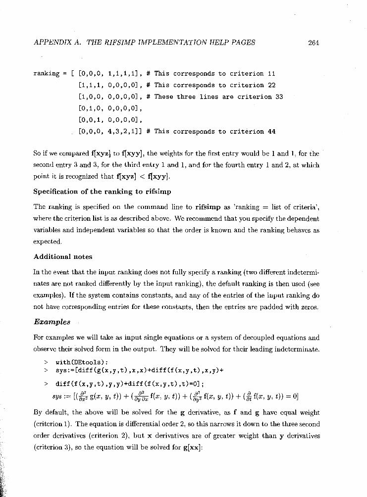
APPENDIX A. THE RIFSIMP IMPLEMENTATION HELP PAGES
ranking = [ [O,O,O, 1,1,1,1], # This corresponds t o c r i t e r i o n 11
[1,1,1, 0,0,0,01, # This corresponds t o c r i t e r i o n 22
[l,O,O, 0,0,0,0], # These th ree l i n e s a r e c r i t e r i o n 33
CO,l,O, O,O,O,Ol,
ro,o,1, O,O,O,Ol,
CO,O,O, 4,3,2,111 # This corresponds t o c r i t e r i o n 44
So if we compared f[xyz] to flxyy], the weights for the first entry would be 1 and 1, for the
second entry 3 and 3, for the third entry 1 and 1, and for the fourth entry 1 and 2, at which
point it is recognized that f[xyz] < f[xyy].
Specification of the ranking to rifsimp
The ranking is specified on the command line to rifsimp as 'ranking = list of criteria',
where the criterion list is as described above. We recommend that you specify the dependent
variables and independent variables so that the order is known and the ranking behaves as
expected.
Additional notes
In the event that the input ranking does not fully specify a ranking (two different indetermi-
nates are not ranked differently by the input ranking), the default ranking is then used (see
examples). If the system contains constants, and any of the entries of the input ranking do
not have corresponding entries for these constants, then the entries are padded with zeros.
Examples
For examples we will take as input single equations or a system of decoupled equations and
observe their solved form in the output. They will be solved for their leading indeterminate.
By default, the above will be solved for the g derivative, as f and g have equal weight
(criterion 1). The equation is differential order 2, so this narrows it down to the three second
order derivatives (criterion 2), but x derivatives are of greater weight than y derivatives
(criterion 3), so the equation will be solved for g[xx]:

APPENDIX A. THE RIFSIMP IMPLEMENTATION HELP PAGES
So how can we solve for f instead? The obvious way is to give f more weight than g by
declaring it as the solving variable by using vars (alter criterion 1):
> rifsimp(sys,Cfl);
tal)le([Solued = [&f(x, Y ax y, t) = -(&g(x, y, t ) ) - (&f(x, Y, t ) ) - (&f(x , Y, t))]])
What if we wanted to solve for the y derivative of f? Well, we could then also weight y
derivatives greater using indep:
> rifsimp(sys,Cfl, indep=Cy,xl); a2 a2 a2 a table([Solved = [W f(x, Y, t ) = -(= g(x, Y, t ) ) - (- f(x, Y, t)) - (E f(x, Y, t))]])
Good, but what if we want to solve for the t derivative of f. This is an unusual example
because we are solving for a lower order derivative in terms of higher order derivatives. We
could specify a new ranking that weights t derivatives higher than everything else: > sample-rank: = [ C0 ,0,0 1 , 01 , # Solve for f over g
> [O,ojl,O,O]] :# t derivs are greatest
> ivars:= [x,y,tl :
> dvars: = [f ,gl:
With the above ranking, f is always greater than g, and t derivatives are always greater
than x or y derivatives of any order. We have to declare the order of occurrence in the
command line arguments so that we can match the independent and dependent variables to
the samplerank table. (These are typed in above for visualization.)
> rif simp (sys, dvars , indep=ivars ,ranking=sample-rank) ; a a2 table([Solved = [%f(x, Y, t) = -(8Srg(x, Y, t)) - (&f(x, Y, t )) - (&f(x, Y, t))ll)
Note: We did not specify a full ranking, but instead specified as much as we required, then
let the default ranking take over.
Note that a ranking like the one above is natural for certain classes of equations. As an
example, consider the heat equation u[t] = u[xx]+u[yy]+u[zz] where the form of the
solved equation is only physically meaningful when solving for the time derivatives in terms
of the space derivatives, even when the space derivatives are of higher differential order.

APPENDIX A. THE RIFSIMP IMPLEMENTATION HELP PAGES 266
As a final example, we construct a strange ranking that weights t derivatives twice as heavily
as x derivatives. This is done for the following: > sys:=[diff (f (x,t) ,x,x,x)+diff (f (x,t) ,t)+diff (f (x,t) ,x,x) ,
> [0,1,0,01] :# t derivs are greatest

APPENDIX A. THE RIFSIMP IMPLEMENTATION HELP PAGES 267
A.8 rifsimp[cases] - case splitting and related options
Description
What is a Case Split?
If an input system is nonlinear with respect to any of its indeterminates (including con-
stants), case splitting may occur.
As an example, consider the ODE in u(t): u'-a u" = 0. rifsimp can only isolate the
leadillg indeterminate u" when a <> 0. Unfortunately, we do not know if this condition
holds, so two possibilities result; either a <> 0 or a = 0.
Consider as a second example the equation u'^2 a-u'-uA2=0. rifsimp needs to isolate the
highest power of the leading derivative, u'^2 which introduces the same two possibilities as
for the first example. This second type of pivot is called the initial of the equation.
This prompts the following definitions:
Pivot
The coefficient of the highest power of the leading indeterminate in an unsolved equation.
It is not known whether this coefficient is nonzero or whether it vanishes with respect to
the resulting system.
Case Split
I A case split in the rifsimp algorithm is the separate handling of the cases of nonzero or
zero pivot during the solution of an equation in the system. By default (without casesplit
on), only the nonzero case is explored.
In the u[t]-a u[tt] = 0 example, the pivot is a, and the generic a <> 0 case is handled by
default.
Exploring All Cases
For some systems, a simplified result for all cases is required. To obtain this, use the
casesplit option. Specification of casesplit in the arguments to rifsimp tells it to examine
all cases in the following way:
Proceed to find the generic solution by assuming that all pivots are nonzero. After each

APPENDIX A. THE RIFSIMP IMPLEMENTATION HELP PAGES 268
solution is found, back up to the most recent nonzero assumption, change to a zero assump-
tion, and proceed to find the solution under this new restriction. The process is complete
when no nonzero assumptions are left to back up to.
The result is a tree of disjoint cases, with the simplified forms presented in a table. Each
case is stored as a numbered entry in the output table, having all the standard entries,
along with an entry called Case that can be used to reconstruct a tree of case splittings
using t2he caseplot command. This Case entry is a list of assumptions made to obtain the
answer for that case. Each assumption is a two or three element list, the first element is the
assunlption made, the second is the derivative being isolated that required the assumption,
and if the third entry is present, it indicates that is was later found that the assumption
is always true, so the assumption does not represent a true case split of the problem, but
rather a false split.
There are three options below that mildly alter this behavior, and these are the faclimit,
factoring, and grobonly options. The first two allow pivots to be introduced to the system
that do not necessarily occur as the coefficient of a specific leading derivative. When one
of these pivots occur, then the second element of the assumption is the name of the option
(rather than the leading derivative). The third option, grobonly, has the effect of introduc-
ing fewer pivots (as equations that are nonlinear in their leading derivative, such as the equa-
tion in the second example at the top of this page, do not directly introduce case splittings),
but has the disadvantage that a less efficient nonlinear equation handling method (pure
I Groebner basis) must be employed. For more detail on the output see r i f simp [output 1, and for more detail on nonlinear equation handling see r i f simp Cnonl inear l .
Case Restrictions
Two options can be used to limit or restrict which cases are explored:
1) casesplit=['<>','=','< >'I This option turns on casesplit and gives the start of the tree to be examined. It is used
primarily for repeating a calculation, or for avoiding particularly difficult cases. Note: A
rerun of the system with additional equations is likely to change the order of the pivots,
so this option is only reliable for the same input as the initial calculation. If a calculation
for a specific case is to be repeated with additional equations, it would be better to append
the assumptions made in the Case list to the original system, and run rifsimp with the

APPENDIX A. THE RIFSIMP IMPLEMENTATION HELP PAGES
combined system.
This option is used to limit the cases being examined based on the solution space dimension
of the linear part of the current system. Though the dimension of the solution space is not
know11 until the computation is complete, an upper bound is available by looking at the
current Solved equations. Note: In the presence of nonlinear constraints, the computed
dimension represents an upper bound on the dimension of the case. This could be used, for
example, to find all forms of a second order ODE that are related by a Lie-point transforma-
tion to the equation y" =0, by setting the minimum free parameters of the Lie-determining
system to 8. The minimum dimension can be specified in a number of ways, including some
shortcuts:
Minimum of n free 0-dimensional parameters in
the dependent variables in vars.
mindim= [v , n] Minimum of n free 0-dimensional parameters in
the dependent variables v (v is either a
dependent variable name or set of more than one).
mindim= [v , n , dl Minimum of n free d-dimensional parameters in
the dependent variables v, where v is as above.
mindim= Ccl ,c2, . . .I Here c1 ,c2, . . . are conditions of the Cv ,n,dl type.
When this option is used, a dimension entry is also provided for each case in the output
system. See the information in rif simp [output] for more detail.
Note: When using multiple specifications, each must be a full specification defining the
number, the dependent variables, and the dimension of the required data.
If any of the input conditions fail, computation is halted on the current case, it is tagged
with the status "free count fell below mindim", and the computation proceeds to the next
case.
Pivoting and Pivot Selection

APPENDIX A. THE RIFSIMP IMPLEMENTATION HELP PAGES 2 70
The rifsimp algorithm proceeds by putting as many PDEs into solved form as possible
without introducing new pivots. When it has reached a point where none of the remaining
unsolved equations can be solved without the introduction of a pivot, it must then decide
which equation to solve. By default, rifsimp chooses the leading linear unsolved equation
that is smallest in size, but this behavior can be modified by the pivselect option described
below. The new pivot for the chosen equation then results in a case split if casesplit is set,
otherwise exploration of only the nonzero (generic) case if casesplit is not set. If none of the
equations are leading linear, then no standard pivot can be found, so rifsimp then attempts
to factor the leading nonlinear equations searching for factors that do not depend on the
leading derivative. If these are found, then the smallest factor (based on the Maple length
function) is chosen, and a "factor" split is performed. This behavior can be modified
through use of the factoring option described below. If nonlinear equations remain, then
the coefficient of the highest degree of the leading derivative in the equation (the initial of
the equation) is split on if initial has been specified (see below) or if grobonly has not
been specified (see rif simp [nonlinear] ) .
The following options relate to pivoting and to the control of pivoting in the course of the
algorithm:
During the course of a computation, rifsimp proceeds by performing as much elimination as
possible before introducing a pivot. Once no further elimination can be done, a pivot must
be introduced, and there is generally more than one possible choice. There are currently six
possible choices for pivot selection:
"smalleq" Choose the pivot belonging to the smallest
equation (based on the Maple length function).
This is the default.
"smallpiv" Similar to "~malleq'~, but the length of the
pivots are compared instead.
Choose the pivot for the equation with
leading derivative of lowest rank. Ties

APPENDIX A. THE RIFSIMP IMPLEMENTATION HELP PAGES
"mindim"
["smalleq" , varsl
["lowrank" ,vars l
a re broken by equation length.
Choose the pivot f o r the equation with
leading der iva t ive t h a t w i l l reduce t h e s i z e
of t he i n i t i a l da t a by the grea tes t amount.
This opt ion can only be used i n combination
with t h e mindim option described above.
Same a s "smalleq" above, but it only looks a t
equations with leading derivat ives i n the
vars sequence.
Same a s "lowrank" above, but it only looks a t
equations with leading derivat ives i n t he
vars sequence.
The choice of a pivoting strategy can significantly affect the efficiency of a computation for
better or worse. In addition to efficiency considerations, the selection of different pivoting
strategies can also simplify the resulting case structure, though the choice that gives the
best case structure is highly problem dependent.
The "smalleq" and "smallpiv" options are generally focussed on efficiency. "smalleq" makes
the computation more efficient by selecting smaller equations for splitting, while "smallpiv"
makes the computation more efficient by introducing smaller pivots.
The "lowrank" and "mindim" options are focussed on keeping the number of cases to a
minimum.
2) nopiv= [varl , . . .] This option gives a list of all variables and constants that cannot be present in pivots.
This is most useful for quasi-linear systems for which the linearity of the resulting system
is of greatest importance. This may also have the effect of reducing the size of the case
tree in these systems. The unsolved equations are then treated as fully nonlinear (see
r i f simp [nonlinear] ) .

APPENDIX A. THE RIFSIMP IMPLEMENTATION HELP PAGES 2 72
Typid ly the pivot chosen is the coefficient of the leading indeterminate in the equation.
In tho event that the leading indeterminate is itself a factor of the equation, and this same
leadiug indeterminate factor occurs in <n> or more equations, then it is chosen as the pivot
rather than as the coefficient. This is most useful for Lie determining systems having many
inconsistent cases, since in these systems, many equations of this form typically occur during
the calculation. The answer may be obtained without this option, but it can significantly
reducc the number of cases returned.
As briefly described above, by default equations that factor are split if one of the factors
does r~ot depend upon the leading derivative of that equation. This option can be used to
modify that behavior based on the value of desc used in the factoring option:
nolead This i s the d e f a u l t . Only s p l i t on a f a c t o r
i f it does not contain t h e leading der iva t ive
of the equation.
a l l S p l i t on any f a c t o r s , even i f they contain t h e
leading de r iva t ive .
none Do not perform fac to red s p l i t t i n g .
In any event, the factoring pivots are always the last to be considered (i.e. faclimit and
regular pivots are used if available). Note: factoring="all" should be used with cau-
tion as it has the potential to significantly increase the number of cases returned. Note:
factoring=" none" can result in non-termination for some nonlinear problems.
5 ) pivsub
When introducing a new pivot, attempt to reword that pivot as a new dependent variable
when it is advantageous to do so. For example, if the new pivot is a(x)+b(x)-c(x,y),
then rifsimp creates a new dependent variable, say Fl(x,y), and adds a n equation to the
system indicating that Fl(x,y) = a(x)+b(x)^2-c(x,y). The ranking would be arranged
such that the new equation would be solved in terms of an existing indeterminate in the
pivot, and the overall effect would be to make the new pivot a single-term expression.

APPENDIX A. T H E RIFSIMP IMPLEMENTATION HELP PAGES 273
The primary advantage of this strategy is that, after introducing a pivot, the solution
procetlure usually results in the occurrence of that pivot and its derivatives, sometimes to
a high polynomial degree. Leaving the pivot in its regular form can result in extensive
expression swell, whereas the reworded pivot remains quite small and manageable.
The now dependent variables are chosen as F.(i),F.(i+l), and so on, where i is larger than
the largest occurrence of an F.(j) in the present system, and is not globally assigned.
6) initial
This option only applies to systems which have nonlinear Constraint equations in their
output. The initial is the coefficient of the highest power of the leading derivative in a
polynomially nonlinear equation (the leading nonlinear derivative). For example, in the
equation u[x] ̂ 2*u+u[x] ̂ 2+u[x] +u-1, the initial is the coefficient of u[x] -2, which is
u+l. By default, rifsimp splits on the initial, unless grobonly is specified (in which
case it does not need to), introducing additional cases in the output. With these additional
cases, rifsimp isolates the leading nonlinear derivatives in the Constraint equations. When
grobonly is not specified, only the form of the Constraint output is different.
Note: These options do not require that casesplit be on, but are typically most useful in
that situation.
0 t her Case-related Options
Another option that is also related to case-splitting is the gensol option, which may return
multiple cases for some problems:
This option indicates that the program should explore all cases that have the possibility of
leading to the most general solution of the problem. Occasionally it is possible for rifsimp
to compute only the case corresponding to the general solution of the ODEIPDE system.
When this option is given, and this occurs, rifsimp will return the single case corresponding
to the general solution. When it is not possible for rifsimp to detect where in the case tree
the general solution is, then multiple cases are returned, one or more of which correspond to
the general solution of the ODE/PDE system, and others correspond to singular solutions.
For some particularly difficult problems, it is possible that the entire case tree is returned.
Note: this option cannot be used with the casesplit,casecount, pivsub, and mindim

APPENDIX A. THE RIFSIMP IMPLEMENTATION HELP PAGES
Examples
> with(DEtoo1s):
Suppose we have the ODE shown below. We want to determine conditions on g(y(x)) and
f(x) that allow the equation to be mapped to y" = 0 by an invertible change of variables of
the form Y=Y(x,y), X=X(x,y). It is known that the equation can be mapped to yV=O
if the Lie group of the equation is &dimensional. This is the perfect opportunity to use the
mindim option in combination with cases, to tell rifsimp that we are only interested in
cases with 8 dimensions or more:
> ODE1 : =dif f (y(x) ,x ,x)+g(y(x)) *dif f (y(x) ,x)+f (x) *y(x) ;
ODE1 := (&Y(x)) + %(Y(x)) (& ~ ( 4 ) + f ( 4 Y(X)
We can use the DEtools odepde command to generate the determining system for this
ODE, and we obtain the following:
> sysl :=[coeff s(expand(odepde(ODE1, [xi(x,y) ,eta(x,y)], y(x)) 1 •÷-yl)l;
> caseplot (ansl) ;
Issuing the caseplot command above would show that there is one case for which this occurs.
This case is given by:
> copy(ansiC31);

APPENDIX A. THE RIFSIMP IMPLEMENTATION HELP PAGES
As a demonstration of the faclimit option, consider the following system: > sys2: = [eta(x,y) * (3*f (x)+2*g(x)-h(x)),
The regular case-splitting strategy produces an undesirable result for this system, namely
more cases than required to describe the system:
> ans2-1 :=rif simp(sys2, [eta] , casesplit) ;

APPENDIX A. THE RIFSIMP IMPLEMENTATION HELP PAGES 276
uns2-1 := table([
1 = table([Solved = [q(x, y) = 01, Pivots = [%2 # 01, Case = [[%2 # 0, q(x, y)]]]), 2
Pivots = [h(x) - 1 # 01, Case = [[%2 = 0, q(x, Y)], [%1 = 0, d x , Y)], [h(x) - 1 # 0, V(X, Y)]] ]) ,4 = table([SoEved = [f(x) = 1, g(x) = -1, h(x) = I],
Case = [[%2 = 0, q(x, Y)], [%I = 0, q(x, Y)], [h(x) - 1 = 0, q(x, Y)II
I), casecount = 4 1) 761 := 4 g(x) + 7 h(x) - 3 %2 := 3 f(x) + 2 g(x) - h(x)
So wc get 4 cases. Now set faclimit set to 2:
> ans2,2:=rifsimp(sys2,Cetal,casesplityfaclimit=2~;
ans2-2 := table([l = table([Solved = [f(x) = l,g(x) = -1, h(x) = 11,
Pivots = [q(x, y) # 01, Case = [[q(x, y) # 0, "faclimit"]]
I ) , 2 = table([SoZved = [q(x, y) = 01, Case = [[q(x, y) = 0, "faclimit"]]]), casecount = 2
I ) So although both ans2-1 and ans2-2 equally valid, it is clear that ans2-2 would be pre-
ferred.
As an example of the factoring option, consider the following purely algebraic system:
> sys := [x^3-7*~+61;
sys := [a3 - 7x + 61 With default options, we obtain
> rif simp (sys , casesplit) ; table([Constraint = [x3 - 7 x + 6 = 011)
With full factoring enabled, we obtain
> rifsimp(sys,casesplit,factoring=all);

APPENDIX A. THE RIFSIMP IMPLEMENTATION HELP PAGES
table([l = table([Solved = [x = 21, Case = [[x - 1 # 0, "factor"], [x + 3 # 0, "factor"]]]), 2 = table([Solved = [x = -31, Case = [[x - 1 # 0, "factor"], [x + 3 = 0, "factor"]]]),
3 = table([Solved = [x = 11, Case = [[z - 1 = 0, 'Lfactor7y]]]), casecount = 3 I)
So we see that the system has been split into three disjoint cases. Also note that the Case
entries describe the path the computation took, and there are no Pivots entries. This is
because the pivots resulting from the case splits are identically satisfied for each case.

APPENDIX A. THE RIFSIMP IMPLEMENTATION HELP PAGES 278
A.9 rifsimp[nonlinear] - information and options specific to
nonlinear equations
Description
Leading nonlinear equations
This help page explains how rifsimp handles equations which are polynomially nonlinear
in thcir leading indeterminate (called leading nonlinear equations), or equations that are
leading linear, but have a coefficient that depends on pivot restricted variables (see nopiv
in r i f simp [cases]).
As all example, consider the equation u[tt] u-u[t]^2 = 0. This equation is linear in its
leadiug indeterminate, so as long as u can be present in a pivot it will be handled through
case splitting rather than nonlinear equation handling (see r i f simp [cases]). Conversely,
the equation u[tt] ̂ 2-u[t] = 0 is leading nonlinear, and is always handled through the
nonlinear methods described here.
During the course of the computation, nonlinear equations are always differentially simplified
with respect to the linear equations of the system, but they are also algebraically simplified
with respect to each other. This simplification process resembles an algebraic Groebner
basis, but takes the inequations (pivots) of the system into account, and does not compute
algebraic S-polynomials. Use of this set of equations allows recognition of, and elimination
of redundant equations, and produces a more compact representation (due to the use of
pivots and lack of S-polynomials).
In order to perform the algebraic simplification of these nonlinear equations, a monomial
ordering must be imposed for all possible nonlinear terms. This is simply chosen to be pure
lexicographical ordering with respect to the ordering imposed on the linear derivatives.
For example, the equation u[xx]^2 u[x]+u[xx]^2 u-u[xIA2-u*2 for a system in which
u [x] +u < > 0 holds is algebraically solved for u[xx] ̂ 2 giving the nonlinear relation:
Note: during the course of the algorithm, when nonlinear equations are encountered, case
splitting is performed on the coefficient of the highest degree of the leading derivative each
equation. This coefficient is called the initial of the equation. So for the example above, the

APPENDIX A. THE RIFSIMP IMPLEMENTATION HELP PAGES 279
initial is u[x]+u. If there was no condition on u[x]+u, then rifsimp would split into the
cases u[x]+u<>O and u[x]+u=O. This can increase the number of cases in the output,
but is required for the proper functioning of the more compact nonlinear equation handling
algorit,hm, so if this splitting is not desired, pure Groebner basis methods can be used
instead with the grobonly option.
If leading linear equations with usable pivots are found in the algebraically simplified set,
rifsimp removes them from the set, and treats them using leading linear methods (i.e. isola-
tion of the leading derivative and pivoting, differential substitution, and linear integrability
conditions) .
Differontial consequences are enforced by the spawning (differentiation with respect to each
independent variable) of each equation, which naturally results in leading linear equations.
Before algorithm completion, rifsimp forms an algebraic Groebner basis over the leading
nonlinear equations, spawning any new relations that appear as a result of S-polynomials.
This step is necessary to ensure that all differential consequences of the leading non-linear
equations are accounted for, so that the set of nonlinear constraint equations returned by
the algorithm can be viewed as algebraic (not differential) constraints.
Of course, Groebner basis computations require a ranking of monomials in a system. By
default the ranking is chosen as total-degree order with ties broken by inverse lexicographical
order (otherwise known as grevlex). The allowed rankings for rifsimp are quite flexible,
but require some knowledge of rankings (please see r i f simp [ranking], and look at the
Groebner Rankings description below).
Control options
There are four options used to control how rifsimp handles leading nonlinear equations.
The spoly and spawn options limit what is done in the algorithm, and thus they generally
return an incomplete answer. Unfortunately, these options are needed in some cases as
highly nonlinear ODE/PDE systems may have to perform a Groebner basis of a large
number of equations in a large number of indeterminates. Though the process is finite, it
can be extremely time consuming, and may not return the result for days (weeks, months,
etc.). These options allow rifsimp to return a result that can be further processed using
other tools, such as hand integration or resultants, to obtain the final result.
1) grobonly

APPENDIX A. THE RIFSIMP IMPLEMENTATION HELP PAGES 280
This option tells rifsimp to only use Groebner basis simplification of the nonlinear equations
in the course of the algorithm instead of using the algebraic simplification described above.
This has the potential to decrease the number of cases in the output, but caution should be
used with this option, as rifsimp works with only part of the system at any one time, so
use of full a Groebner basis on only a partial system can often lead to inefficiency.
2) checkempty
This option tells rifsimp to attempt to determine, on the completion of the calculation (or
the completion of each calculation when dealing with cases) whether the resulting system
contains any solutions. These empty systems do not occur for linear problems, but when
algebraic constraints and pivots are both present for a system, then there is a possibility
that the resulting output has no solution. For a simple example, see the last problem in
the examples section below. Caution should be used for this option also, as the checking
process can be quite expensive.
This option indicates whether to generate S-polynomials during the Groebner basis algo-
rithm (default is true). Setting spoly=false has some risk associated with it, as if nonlinear
equations are present in the output, then it is possible that not all consequences of these
equations have been obtained (hence they are placed in the DiffConstraint list rather than
the Constraint list). If an orderly ranking is used ( see rifsimpCrankingl), and spawn
is set to t rue (see below), then only algebraic simplifications remain, but these may still
result in an inconsistent system when considered with the Pivot equations.
Note: By algebraic simplifications we mean that there are no further integrability conditions
that can result once the system is algebraically simplified. Differential reduction of leading
linear equations can still occur.
Indicates whether to perform a differential spawn of nonlinear equations (default is t rue) .
A differential spawn simply means taking the derivative of an equation with respect to all in-
dependent variables. Setting this to false allows rifsimp to ignore differential consequences
of the polynomially nonlinear equations. This is only useful if rifsimp is being used as a
single step of a different calculation, since an incomplete answer may be obtained. When
spawn=false, all nonlinear equations are placed in the DiffConstraint list rather than

APPENDIX A. THE RIFSIMP IMPLEMENTATION HELP PAGES
the Constraint list to indicate that the answer may be incomplete.
Groebner rankings 1
A Grocbner ranking is a ranking defined on the set of all monomials in the indeterminates
of a system of equations. For example, if the indeterminates were x, y, and z, a ranking
would be able to order the monomials x*y^2*z, xe3*y^2, xA2*y*z^2, x^2*y*zA4, and
determine a leader. The determination of this leader is vital to the completion of a Groebner
basis, and different rankings can give drastically different bases for the same input system.
Algebraic monomial rankings
There are a number of standard Groebner basis rankings available for algebraic systems of
equations. The rankings described below can be used in rifsimp. Each ranking is described
as a comparison of two monomials:
1) Total-degree ranking
This only defines a partial ranking; that is, there can be ties for different terms. It looks at
the degree of each monomial in all indeterminates (the total degree), and if the total degrees
of the monomials are different, the one of larger degree is ranked higher.
2) Lexicographic ranking
Given an ordered list of indeterminates, lexicographic ranking compares the degrees of the
two monomials in each indeterminate in turn. If the degree of one monomial is greater than
the other in that indeterminate, then it is ranked higher.
3) Inverse Lexicographic ranking
This ranking looks at the ordered list of indeterminates in reverse order, and compares the
degrees of the two monomials in each indeterminate in turn. If the degree of one monomial
is lower than the other in that indeterminate, then it is ranked higher.
It is important that a ranking is deterministic. That is, given two different monomials
it is always possible to rank one higher than the other. Since a total-degree ranking is
not deterministic, it must be followed by either a lexicographic or an inverse lexicographic
ranking.
As an example we look at all monomials in x, y, and z up to total degree 3 and rank them
using the rankings described above.

APPENDIX A. THE RIFSIMP IMPLEMENTATION HELP PAGES
Total Degree followed by Lexicographic on [x,y,z]
Total Degree followed by Lexicographic on [z,y,x]
Total Degree followed by Inverse Lexicographic on [x,y,z]
Pure Lexicographic on [x,y,z]
Simple algebraic rankings in rifsimp
The rankings for Groebner basis computations in rifsimp are specified by the grob-rank
= [criterion list] option. If all that is needed is an algebraic ranking as described above
(for the indeterminates in the order described by the linear ranking) the criterion list can
simply be given as below:
grob-rank=[[l,deg,none], [l,ilex]]
This says to use algebraic total-degree ranking followed by inverse lexicographic ranking
(this is the default).
grob-rank=[[l,deg,none], [l,lex]]
Use algebraic total-degree ranking followed by lexicographic ranking.
grob-rank= [[1 ,lex]]
Use pure lexicographic ranking.
The criterion lists may seem a bit verbose for what they need to accomplish, but far more
detailed rankings are available (see Groebner Rankings 2 below).
Though the pure lexicographic ranking produces a more desirable result, total-degree / inverse lexicographic ranking was chosen as the default as it was in general (by experiment

APPENDIX A. THE RIFSIMP IMPLEMENTATION HELP PAGES 283
on a number of ODE/PDE systems) the least expensive in time and memory.
Groebner Rankings 2: a different point of view
The niain thing to note is that all the types of monomial rankings previously discussed can
be viewed as looking at the degree of one or more indeterminates between the two monomials
being compared.
For example, total degree followed by lexicographic ranking (for the x,y,z example) looks at
the degree of the monomials in x,y,z, then in x, then in y, then finally in z. Total degree
followed by inverse lexicographic ranking looks at the degree of the monomials in x,y,z,
then x,y, then x,z, then y,z.
So now that we are dealing with differential systems, it may be desirable to rank inde-
terminates based upon other criteria such as their differential degree, dependent variable,
differentiations, etc. This can be accomplished in rifsimp.
Classification of linear ranking criteria
As a first step, all linear differential ranking criteria are classified.
diffdeg
dif f var
depvar
other
all
none
any criterion comparing differentiations of more than one
independent variable
any criterion involving differentiations of a single independent
variable
any criterion only involving dependent variables
any criterion which mixes independent and dependent variables
all possible criteria
no criteria
For more detail about criteria, please see rif simp [ranking]. In that help page, an example
of the diffdeg classification is given by criterion 2, diffvar by criterion 3, and depvar by
criterion 1 and 4.

APPENDIX A. THE RIFSIMP IMPLEMENTATION HELP PAGES 284
Theso classifications, which actually refer to a specific part of the linear ranking, allow the
definition of equivalence classes for the derivatives. The monomial ranking then takes the
degrco of each monomial in derivatives of the same equivalence class.
Definition of the criteria for grob-rank
With Lhe above information we can now construct a differential monomial ranking as an ex-
amplo. Suppose we define our first criterion as [l,deg,diffdeg]. This describes equivalence
classos based upon the differential degree of the derivatives. Consider a system containing
the dependent variable f(x,y) and all derivatives up to second order, and using the default
linear ranking for differential degree (all differentiations have equal weight). This defines
the following equivalence classes:
Now when comparing two monomials, the degree of the monomials in each equivalence class
is considered in turn, and if they are different, the one with greater degree is ranked higher.
Here are a few examples:
f [xxlA2*f Cxyl *f [yl *f < f Cyyl-4 Degree i n second order d e r i v a t i v e s
i s 3 < 4
f [xyl *f [yyl < f 1 ~ x 1 ~ 3 Degree i n second order d e r i v a t i v e s
is 2 < 3
f [xyl^2*f [yyl *f [yl *f -20 < Degree i n f i r s t order d e r i v a t i v e s
f Cyy1^3*f [XI *2*f - 3 i s 1 < 2.
This does not fully determine a ranking, since if there were (for example) two terms that
were fourth degree in second order derivatives, this criterion would regard them as equal.
To fully specify the monomial ranking, we could add another criterion of the lex or ilex
type. If we added a lex criterion, namely [l,lex], then we would be looking at the degree of
the monomials in the indeterminates in their linearly ranked order. Again using the default
for the linear ranking, and considering the f(x,y) system up to second order we would get
the following:

APPENDIX A. THE RIFSIMP IMPLEMENTATION HELP PAGES 285
This is presented in the same manner as the equivalence classes for the degree-type monomial
rankiug.
fCxxl -2 fCxy1 fCy1 f < fCxx1-3 f [ x l f Degree in fCxxl is 2 < 3.
f [xxl-2 f Cyyl < f Cxxl-2 f Cxyl Degree in f Cxy] is 0 < 1.
f Cxyl-2 f [yyl f Cxl f Cyl f < Degree in f Cxl is
f cxy1-2 f Cyyl f Cxl-2 f 1 < 2 .
In summary, one should consider all the criteria as a list of equivalence classes, for which the
degreo of the monomial in the indeterminates of the equivalence class determines the relative
monornial ranking. For grob-rank= [[1 ,deg,diffdeg] , [1 ,lex]] , and the above examples, the
list of equivalence classes is given as follows:
[{f [xx], f Cxyl, f Cyyl3, Cf Cxl, f Cyl3, If), Cf Cxxl3, Cf Cxy13, Cf [ Y Y ] ~ , CfCxl3, Cf Cyl), (f313
One final detail - a bit more flexibility
You may have noticed that there is always a 1 present as the first element of each criterion,
but it is not discussed. This allows a bit more flexibility in the specification of the ranking,
as it allows for nesting of the criteria.
Consider again the earlier example where the criterion was specified as [[l,deg,diffdeg] ,[l ,lex]] .
Based on the above description, if the higher derivatives are of equal degree in each order of
derivative, then the degree of the lower order derivatives may be used to break the tie. This
may not be what is desired. Suppose one wants to examine the degree in the higher-order
derivatives, and if they are equal, to compare the higher-order derivatives lexicographically.
This can be accomplished through nesting. Any increase in the first element (integer) of a
criterion from the prior criterion indicates that the new criterion should be nested inside
the prior.
Consider our earlier example system with the new nested ranking [[1 ,deg,diffdeg] , [2 ,lex]] .
This would have the effect of changing the order of the combined equivalence classes to the
following:
[{f [xx], f [xyl, f Cyyl3, Cf Cxxl3, Cf Cxyl3, Cf Cyyl3, Cf 1x1 3 f [yl39 {f[xl) , CfCyl3, Cf3, Cf3l

APPENDIX A. THE RIFSIMP IMPLEMENTATION HELP PAGES 286
This tdls rifsimp to consider the degree of the monomial in second order derivatives, then
in each second order derivative in turn, then do the same for first order derivatives, etc.
Here are a few examples:
f [xxl-2 f [xyl f [yl f < f [yyl-4 Degree in second order derivatives
is 3 < 4.
f Cxyl -2 f Cyyl f [yl-6 < f Cxxl-3 Degree in f [xx] is 0 < 3*.
f Cyyl-3 f Cyl-2 f-20 < Degree in first order derivative
f [yyl-3 f Cxl-2 f -3 f[xl is 0 < 2*.
The comparisons with * will give different results for the non-nested ranking.
Examples
The following example arises from the parameterization of an ellipse (where we have used
PDEtools [declare] to compact the output and display the derivatives in primed notation.
> with(DEtoo1s): with(PDEtoo1s):
> declare(x(t1 ,y(t) ,z(t) ,prime=t) ;
x ( t ) will now be displayed as x
y ( t ) will now be displayed as y
derivatives with respect to : t of functions of one variable will now be displayed wi\
t h ' z ( t ) will now be displayed as z
> sysl:=[diff (y(t) ,t)-x(t)-2-x(t),
> y(t)"4-2*y(t>~2*diff(z(t),t)+diff(z(t),t)~2
> -y(t)"2+2*diff(z(t),t),
> diff (x(t) ,tIA2+2*y(t)*diff (x(t) ,t)+y(t)̂ 4] ;
sys l := [y' - x 2 - x, y4 - 2 y2 2' + z12 - y2 + 2 z 1 , x12 + 2 y ~ ' + ~ ~ ]
Calling with the default ranking gives the following:

APPENDIX A. THE RIFSIMP IMPLEMENTATION HELP PAGES 287
ansl := table([Case = [ [ X I + y # 0, x"], [-y2 + z' + 1 # 0, 2"]],
Pivots = [x' + y # 0, -y2 + zr + 1 # 01, Constraint = [xr4 + 2 zt2 xt2 + z14 + 4 xr3 y
x ( 2 x + 2) y3 + x ( x + 1) x1 Solved = [x" = -
x l + y 1
I ) So we have isolated ODE for y', x" and z", and four constraints involving x, y,x' , and z'.
> nops (ans l [Constraint] 1 ;
If instead we want to perform an elimination of x, then z , then y , we can specify this
through use of a lex ranking for the algebraic problem.
> ans2 : = r i f simp(sys1, C Cxl , Czl , Cyl I ,grab-rank= C C l , l e d 1 ) ;
ans2 := table([Case = [[-2x - 1 # 0, X I ] , [y" y # 0, X I , [-y2 + z' + 1 # 0 , z"],
[ ( I + 4 Y ' ) (4Y4 Y' + Y 4 - Y112) # 0, ~ " ' l l , Pivots = [-ytt2 - y4 - 4 y4 y' # 0, yn # 0, -y2 + z' + 1 # 0 , 4 y4 y' + y4 - ytt2 # 01,
Constraint = [y4 - 2 y2 z' + z12 - y2 + 2 z' = 0, I 1'2 2 112 2 1'2 4 112 4 I -16y y y - 4 y y + y 1 ' ~ + 2 y y + 8 y y y + y 8 + 8 y 8 y ' + 1 6 y 8 y ' 2 =
01
1 2y1'y+ y'12 + y4+4y4 y' Solved = [ x = - - , ztl = - - 2 y 3 y ' + 2 y z ' y 1 + Y y '
4 Y" Y y2 - z' - 1 ,
I ) so now we have isolated ODE for x and z", an ODE in y"' in terms of y alone, and two
constraints involving z',yV ,y' and y
For an example of the use of the grobonly and checkemp ty options we consider the
following algebraic system:

APPENDIX A. T H E RIFSIMP IMPLEMENTATION HELP PAGES
If wc (:all rifsimp with this system, and the inequation aA2+b<>0 we get:
> ans3-1: ==if simp ( Cop (sys3) , a^2+b<>01 ,nopiv= [bl , casesplit, grobonly) ;
ans3-1 := table([Pivots = [b + a2 # 01, Constraint = [ a 3 - c = 0 , a c + b 2 + 2 b a 2 = 0 , 2 b c + a 2 c + a b 2 = 0 , -3bac+b3-2c2=01
I ) But with the additional option 'checkempty' we get
> ans3~2:=rifsimp([op(sys3),a~2+b<>O],nopiv=[b],casesplit,grobonly,
> checkempty) ;
ans3-2 := table([status = "system is inconsistent"])
because ans3-1 represents an empty case.

APPENDIX A. THE RIFSIMP IMPLEMENTATION HELP PAGES 289
A.10 maxdimsystems - determination of maximum dimen-
sional subsystems of systems of PDE
Calling Sequences
niaxdimsystems(system, maxdimvars)
maxdimsystems (system, maxdimvars, op t ions)
Parameters
system - list or set of ODE or PDE (may contain inequations)
maxdimvars - list of the dependent variables used for the dimension count
o~hons - (optional) sequence of options to control the behavior of maxdimsys tems
Description
The default output of maxdimsystems (modulo *** below) consists of the set of cases
having maximal dimension in maxdimvars, where each member has the form:
[Solved = l i s t , Constraint = l i s t , Pivots = l i s t , dimension = integer]
Solved is a list of the PDE which are in solved form with respect to their highest derivative
(with respect to the given ranking of derivatives), Constraint is a list of the PDEs in
the classvars (any dependent variables not in maxdimvars) which are nonlinear in their
leading derivatives, Pivots is a list of the inequations in the classvars and/or maxdimvars,
and dimension is the maximal degree of arbitrariness in maxdimvars (i.e. the number of
arbitrary constants on which maxdimvars depends).
*** The result is valid provided that the Constraint and Pivots equations have a so-
lution, and also that maxdimvars do not occur in the constraint equations. The user must
check the first condition algebraically (e.g. see Groebner Cgsolvel , and possibly d i f f a lg) .
If the maxdimvars are present in the pivots, then the returned system will have lower
dimension that indicated, and must be handled manually.
Each of the cases is in r i f simp form (a generalization of Gauss normal form to systems of
PDE) and also contains a system of differential equations and inequations in the classvars
characterizing the case. In the same way that the Gauss normal form is determined by a

APPMVDIX A. THE RIFSIMP IMPLEMENTATION HELP PAGES
orderiug of variables, rifsimp form is determined by a ranking of derivatives.
The clcfault ranking is determined by maxdimvars. It can be inferred by the application of
checkrank, and always ranks the classvars and their derivatives lower than all maxdimvars.
The itlaxima1 cases can be determined in many applications where a complete analysis
of all cases is not possible. These cases are often the most interesting, with the richest
proporties, when compared to the relatively uninteresting (but often difficult to compute)
lower dimensional cases.
The options for maxdimsystems consist of the output option (described below), and a
subscl of those for r i f simp, the main subroutine used by maxdimsystems. Of the subset
of rifsimp options available, two that are often used are indep which specifies the inde-
pendant variables, ezcriteria which controls the flow of equations from a fast (ultra-hog)
setting (that can readily lead to memory explosion but sometimes faster calculations), to
a conservative (one equation at a time) setting that can overcome some expression swell
probloms. The complete list is given by:
tosolve, indep, a r b i t r a r y , c l ean , f u l l c l e a n See rifsirnpCoptions1
e z c r i t e r i a , f ac l imi t See r i f simp [adv-options]
mindim, p ivse lec t See r i f simp[casesl
grob-rank,grobonly,checkempty See r i f simp [nonlinear]
Many rifsimp options are not supported by maxdimsystems as their use could produce
misleading results. For example, the rifsimp option c t k t i m e , places a time limit on
rifsimp case computations, and hence could cause maxdimsystems to miss the maximal
case if it takes too long to compute. Conversely, specification of other options are not
supported as they must have a specific value for the maxdimsystems command to function
properly (for example, casesplit must always be on). Other unsupported rifsimp options
include itl, st l , nopiv, unsolved, pivsub, s tore , storeall, spawn, spoly, and casecount.
ou tput = type
The output type can either be set (default) or rif. Note that se t output is easier to read
and manipulate, but cannot be used with the caseplot visualization tool. The rif output
can be used with caseplot, but the output is somewhat more complicated, and is described
in r i f simp[outputl . Note that for the class of problems that maxdimsystems simplifies,

APPENDIX A. THE RIFSIMP IMPLEMENTATION HELP PAGES 291
many of the outputs from rifsimp described in the output page ( such as DiffConstraint
and UnSolve) will never be present in the output.
The maxdimsystems command allows a subset of the rankings available for rifsimp.
Specifically those rankings that are controlled by a partition of the dependent variables in
maxdimvars, and those available by the order of the independent variables in indep. See
rif simp [ranking] and checkrank for an explanation of how to specify rankings based on
these options.
The application of caseplot to the rif-form output of maxdimsystems with the second
argument given as the maxdimvars displays the tree of maximal cases and their dimensions,
also indicating which branches of the tree have less than maximal dimension.
Note that maxdimsystems is essentially a simplified version of the rifsimp interface that
also has the ability to automatically determine the maximum finite dimensional cases or
all infinite dimensional cases for a classification ODEIPDE system. If the dimension of
the solution space is known, multiple conditions on the dimension of the solution space are
needed, or much finer control of the computation is desired, then rif simp could be used
with the mindim option described in rif simp [cases].
References:
G. J. Reid and A.D. Wittkopf, "Determination of Maximal Symmetry Groups of Classes of
Differential Equations", Proc. ISSAC 2000, pp.272-280
G.W. Bluman and S. Kumei, "Symmetries and Differential Equations", Springer- Verlag,
vol. 81.
Examples
> with(DEtoo1s) :
Algebraic systems can be examined with maxdimsystems
> maxdimsystems([ u - a*v = 0, u - c*v = 01, [u,vl>;
{[Solved = [u = cv, a = c], Constraint = [ I , Pivots = [I, dimension = 11)
In the below example, inequations are given in the Pivots list, and the dimension is 2

APPENDIX A. THE RIFSIMP IMPLEMENTATION HELP PAGES
dimension = 2, Constraint = [ ] I ) This next example has a constraint on the classvars present in the result
> maxdimsystems( Cdiff (u(x,y) ,x) - f (x,y)*u(x,y) = 0,
a Wolved = [z u(x, Y ) = f(x, 9) u(x, Y), u(x, Y) = !dx, Y) u(x, Y), gj f(x, 9) = 0,
& g(x, y) = 0 2 f(x, y) = 01, Constraint = [f(x, y)3 - 1 = 01, Pivots = [ I , ' dimension = 11)
In each of the above examples maxdimsys tems picked out the maximum dimensional case.
This is in contrast to rifsimp, with its casesplit option, which obtains all cases.
For the second example, computation with rifsimp using casesplit gives 2-d, 1-d and 0-d
cases, of which the 2-d case is the maximal case from the above example. > ans := rifsimp(C (a(x)-d(x))*diff(u(x),x,x) +
> [ul, casesplit);

APPENDIX A. THE RIFSIMP IMPLEMENTATION HELP PAGES
a2 ans := table([l = table([Case = [[a(x) - d(x) # 0, u(x)]],
Pivots = [a(x) - d(x) # 0]
I), 2 = table([Case = [[a(x) - d(x) = 0, $ u(x)], [b(n) # 0, & u(x)]],
Pivots = [b(x) # 01 I), 3 = table([Case = [[a(%) - d(x) = 0, & u(x)], [b(x) = 0, & u(z)]],
Solved = [u(x) = 0, a(x) = d(x), b(x) = 01
11, casecount = 3 I )
from which the caseplot with initial data counts could be viewed by issuing the command:
One example of practical use of maxdimsystems is the determination of the forms of f(y')
(wherc f(y') is not identically zero) for which the ode yV=f(y') has the maximum dimen-
sion.
where the above symeq is an overdetermined system of PDE in the infinitesimal symmetries
xi(x,y) ,eta(x,y).
So we compute the maximum dimensional case which, is not displayed as it is quite large:

APPENDIX A. THE RIFSIMP IMPLEMENTATION HELP PAGES
from which we see that we have one case, of dimension 8, and it occurs when the displayed
ODE in f(-yl) is satisfied. This classical result is also explored in the ISSAC Proc. article
listed in the references (the primary reference for this command).
The timing above should be compared to the rifsimp full case analysis that takes signifi-
cantly longer, and has a great number of lower dimensional cases: > t2 := time():
> rsys:= rifsimp([op(symeq) ,f (-yl)<>01 , [xi ,eta] , ' casesplit '1 :
> rsys [' casecount 'I ;
11
The overdetermined system for it's symmetries X,T,U is given by

APPENDIX A . THE RIFSIMP IMPLEMENTATION HELP PAGES
l/k(u)*diff (X(u,t ,x) ,u)*diff (k(u) ,u)-diff (diff (X(u,t ,XI ,u) ,u) ,
diff (diff (U(u,t ,x) ,x) ,XI-l/k(u)*diff (U(u,t ,XI ,t)
l/k(u)*diff (T(u,t ,XI ,t)+U(u,t,x)/k(u)^2*diff (k(u) ,u)
-diff (diff (T(u,t ,XI ,x) ,XI-2/k(u)*diff (X(u,t ,XI ,XI
-diff (diff (X(u,t ,x) ,x) ,x)+2*diff (diff (U(u,t ,x) ,u) ,x)+l/k(u)
*diff (X(u,t ,x) ,t)+2*diff (k(u) ,u)/k(u)*diff (U(uytyx) ,XI ,
-2*diff (k(u) ,u)/k(u)*diff (T(u,t,x) ,x)-2/k(u)*diff (x(u,t ,x) ,u)
-2*diff (diff (T(u,t ,x) ,u) ,x) ,
-1/k(u)*diff(k(u),u)*diff(~(u,t,x),u)-diff(diff~~~u,t,x~,u),u),
-2*diff(T(u,t,x),u)l:
At the same time as determining maximum dimensional cases, one can request, through
a partitioning of the maxdimvars, that the dependent variables be ranked in a specific
manner. To always isolate derivatives of U(u,t,x) in terms of the other dependent variables,
one could specify maxdimvars=[[U],[X,T]] . For this problem we would obtain
> maxdimsystems ( [op(sys) ,diff (k(u) ,u)<>O] , [[U] , [X ,TI I ) ;
a a2 7 (& k b N 2 T(u, t , 4 = 07 k(u) = - I Constraint = [ I , Pivots = [& k(u) # 01,
4 k(u)

APPENDIX A. THE RIFSIMP IMPLEMENTATION HELP PAGES 296
Alteruatively we could try to obtain PDE only in U(u , t ,x ) and the classifying function
k(u) 1)y an elimination ranking:
> maxdimsystems ( Cop (sys)
a a2 7 t Z k ( ~ ) ) ~ zU(u , t , x ) = 0, =k(u) = -
4 k ( 4 I , Constraint = [I, Pivots = [& k(u) # 01,
dimension = 5 11 where you can see from the above that we have three PDE for U(u,t ,x) alone (which can
be quite easily solved for U(u,t,x) in terms of a function that is linear in x with coefficients
as integrals in u depending on k(u)).
Both computations show that maximal group is of dimension 5, and occurs when k (u )
satisfies k" = 7/4 (k')^2/k. This is a known result (see the Bluman/Kumei reference).
In determining how a specific ranking will be used in a system, one should consult the
checkrank help page.
The final example demonstrates how to find near-maximal cases, and how to obtain rif-
style output. Say we want all cases having dimension 3 or greater, and we want the rifsimp
output (so we can display the information in a case plot). This can be done as follows: > rif ans : =maxdimsystems ( [op(sys) ,dif f (k(u) ,u) 0 0 1 , [X ,T ,Ul ,mindim=4,
> output=rif) ;

APPENDIX A. THE RIFSIMP IMPLEMENTATION HELP PAGES
rifans := table([l = table([dimension = 3, UnClass = [0 = ~ ( u , t , x ) ( & k ( ~ ) ) ~
k ( 4 ) - 2 U(u, t, 4 ( 6 k ( 4 I 2 k ( 4 + U(% t , 4 (& k ( 4 ) k ( 4 (& 25(4)1, (w Case = [[%4 # 0, U(u, t , x)]], status = "free count fell below mindim", -
I 1 (& k ( 4 ) (& U(u, t , 4 ) , Solved = & ~ ( u , t , x) = - 2 k ( 4 , U(@, 2) =
Pivots = [%3 # O]]),
3 = table([dimension = 5, Case = [[%4 = 0, U(u, t, a)], [%3 = 0, & U(u, t , x)]],
J
casecount = 31)

APPENDIX A. THE RIFSIMP IMPLEMENTATION HELP PAGES
a %l := T(u , t , z) = -U(%t,x) (& k(u)) + 2 (& X(u, t , x ) ) k(u) k ( 4
All cases where the initial data was smaller than the bound are tagged with a status of "free
count fell below mindim". This calculation can then be displayed in a caseplot with the
> caseplot (rif a m , [X , T ,U] ) ;

APPENDIX A. THE RIFSIMP IMPLEMENTATION HELP PAGES 299
A . l l initialdata - find initial data for a solved-form ODE or
PDE system
Calling Sequence
ini tialdata(system,vars)
initialdata(rifresu1t)
ini tialdata(rifresu1t ,vars)
Parameters
system - list or set of polynomially nonlinear PDEs or ODES in solved form
vars - the dependent variables to compute the initial data with respect to
rifresult - a single case result as returned by r i f simp
Description
The initialdata function determines the initial data required to obtain a formal power
series solution for a PDE or ODE system at a point (see r taylor) . The input system
must be in standard or involutive form, so all equations must be of the form derivative
= expression, and there must be no additional relations between the dependent variables
that are not accounted for by the equations of the system. It can be used on any PDE
or ODE system in isolated form, as well as for a single case result output by r i f simp. In
general, all integrability conditions (equality of mixed partials) must be satisfied to obtain
an accurate answer, so it is best to use rifsimp to simplify the system before calculation of
the initial data.
The optional vars argument allows specification of the variables to compute the initial data
of. This option is useful for classzjication problems, where different dependent variables play
different roles in the system. This option also provides a way to specify the variables of a
problem and their dependencies (in the event that one of the dependent variables does not
appear in the Solved list, for example).
The output is given in table form with the Finite entry containing the required zero di-
mensional initial data (constants), and the Infinite entry containing the required higher

APPENDIX A. THE RIFSIMP IMPLEMENTATION HELP PAGES
dimer~sional data (functions).
When the input to initialdata is a rifresult, then additional information is provided on
output. As well as the infinite and finite initial data, the resulting table may contain a
Pivots and/or Constraint entry (if these entries are present in the rifresult) . These
retunwd lists of equations are given in terms of the initial data.
When Constraint equations are present in the result, these equations must be satisfied by
the initial data for the underlying system to be 'well posed'. These Cons t ra in ts must be
accouuted for manually.
Notes:
When not using the rifresult form of the initialdata call, any nonlinear constraints must
be couverted to initial data form and imposed manually.
The initial data required for a system is independent of the right hand side of the solved
form oquations, so for the examples below we may simply ignore the right hand side.
Background Information: Formal Power Series and the ini t ia ldata algorithm
Being able to obtain a formal power series solution of a PDE or ODE system at a point
essentially means that the values of all derivatives of the solution at that point are known,
or can be found through differential relations from the system.
As a simple example, consider the ODE in u(x), u" = u u' (where prime notation is used
to der~ote differentiation). Here the initial data would simply be u(x0) and u'(x0). With
this data and the ODE, we could then determine u" (xO) = u(x0) u'(xO), and from the
derivative of the ODE, we could obtain u"'(x0) = u'(x0)^2+u(xO) u" (xO), and so on.
Knowledge of all derivatives then allows us to write u(x) = u(xO)+(x-x0) u'(xO)+(x-
x0)"2 u(x0) u'(x0)/2+' ...' to any desired order.
As an example of the initialdata algorithm in two dimensions, consider the following sys-
tem:
> sys := [diff (f (x,y) ,x,x,x)=O,diff (f (x,y) ,x,y)=Ol ; a3
sys := [= f(", Y) = 0, & f(", Y) = 01
> initialdata(sys);

APPENDIX A. THE RIFSIMP IMPLEMENTATION HELP PAGES
table([Infinite = [f(xo, y) = -Fl (y)],
F in i te=[D~(f) (xo, YO)=-C1, Di,i(f)(xo, yo) =-C2]
I ) In this case we have one arbitrary function and two arbitrary constants. Plots can be
used to visualize how the initialdata algorithm calculates this data. Consider an integer-
valued graph where the x-axis represents differentiation by x, and the y-axis represents
differcritiation by y. Looking at f[xxx] from our original system, we can place dots at that
value and at all of its derivatives: > d1:=C3,01,C4,01,C3,11,C4,11,C3,21,C4,21,~3,31,C4,31,~3,
Note, for example, that the point (4,l) corresponds to f[xxxxy], which can be obtained
from the differentiation of f[xxx] with respect to x and y. Adding in all derivatives that
are known from the qxy] equation gives the following graph:

APPENDIX A. THE RIFSIMP IMPLEMENTATION HELP PAGES
Now the objective is simply to fill in all missing points. From our graph we can see that
all points of the form (0,i) are missing, which explains the arbitrary function of y in the
answer. This function describes the data for all y derivatives of f. We still require the points
(1,O) and (2,0), which correspond to the arbitrary constants present in the answer for the
values of ax ] and f[xx], as given in the Finite list.
Examples
> with(DEtoo1s):
> sysl:=Cdiff (f (x,y,z) ,x,x)=O,diff (f (x,y,z) ,y)=O,diff (f (x,y,z) ,z)=O] ; a a sysl := [& f(x, y, z) = 0 - f(x, y, z) = 0, , f(x, y, z) = O] ' ay
This system is fully specified if the following derivatives are known.
> initialdata(sys1);
table([Finite = [f(xo, yo, 20) = -C1, & f(x0, yo, ZO) = -C2], Infinite = [1])

APPENDIX A. THE RIFSIMP IMPLEMENTATION HELP PAGES 303
For this next system, the initial data contains a number of arbitrary functions of one variable. > sys2:=[diff (f (x,y,z) ,x,y)=O,diff (f (x,y,z) ,x,z)=O,
table([Finite = U, Infinite = [f(x, YO, zo) = -Fl(x), 8 ~ ( x o , Y, ZO) = - F ~ ( Y ) , & f(xo, YO, Z ) = -F3(~)1
I) For the next system, the initial data contains a number of arbitrary functions of two vari-
ables.
table([Finite = [I, Infinite =
d2 [ fb , Y, 20 ) = -Fl(x, Y), &fb, Yo, 4 = - W x , 4, m f ( x 0 , Y, 4 = 9 3 ( y , 41 I )
Of course, we must include the one-dimensional heat equation.
> sys4:=[diff (u(x,t) ,t)=diff (u(x,t) ,x,x)l ;
d a2 sys4 := [% u(x, t ) = U(X, t)l
> initialdata(sys4) ;
table([Finite = 1, Infinite = [u(x, to) = -Fl(x)]])
This example is a system that contains mixed data: > sys5:=[diff (f (x,y,z) ,x,y,y)=O,diff (f (x,y,z) ,x,z)=O,diff (f (x,y,z) ,y,z,
> z)=OI ; d3 d2 a3
sys5 := [- f(x, Y, 4 = 0, f(", Y, 4 = 0, f(x, Y, 4 = 01
> initialdata(sys5) ;

APPENDIX A. THE RIFSIMP IMPLEMENTATION HELP PAGES 304
2 table([Finite = [&- f(xo, yo, zo) = -Cl],
z DY a Infinite = [f(x, yo, zo) = -Fl(x), &f(x, yo, 10) = E2(x), zf(xo, yo, Z) = - F ~ ( P ) ,
2 &T f(x0, Y, Zo) = - F ~ ( Y ) , f(3.0, Y, PO) = -F~(Y)I
I ) And an example of use of initialdata with a nonlinear rif result:
aZ a2 B Pivots = [= U(X) # 01, Constraint = [( u ( x ) ) ~ U(X) + (% ~ ( 2 ) ) ~ = 01,
Gm? = I b ( 4 # 0, ($ ~ ( 4 ~ 1 , I$ 44 # 0, g3 ~ ( 4 1 1
I ) > initialdata(rif6) ;
table([Pivots = [-C3 # 01, Constraint = [ - ~ 3 ~ -C1 + - ~ 2 ~ = 01, a a2 Finite = [u(xo) = -Cl, u(xo) = -C2, = u(xo) = -C3],
Infinite =
I ) where it is understood that the selected initial data must obey the nonlinear constraint (so
in truth we only have two free parameters) and must not violate the pivots (so -C3<>0,
and as a result -C2< >0) .

APPENDIX A. THE RIFSIMP IMPLEMENTATION HELP PAGES 305
A.12 rtaylor - obtain the Taylor series for an ODE or PDE
system
Calling Sequences
rtaylor(solved, options)
rt;lylor(solved, vars, options)
Parameters
solved - system in solved form
vars - (optional) solving variables of the system
options - (optional) sequence of options to specify the ranking for the solved form, initial
data, and the order of the Taylor series
Description
The rtaylor function uses an output rifsimp form to obtain local Taylor series expansions
for all dependent variables in the ODE or PDE system simultaneously. The Taylor series
output is a list containing equations of the form depvar(indepvars)=Taylor series.
The ranking related options that are accepted by r taylor include the specification of the
vars as a ranking, and the ranking and indep options described in r i f simp [ranking],
r i f simp [optionsl , and r i f simp [adv-options1 .
Note: specification of different vars than those used to obtain the result from r i f simp can
give incomplete results.
The order=n option specifies the order that the Taylor series should be computed to, and
must be a non-negative integer. The default value is 2.
The table resulting from a call to i n i t i a l d a t a can be given as an option to r taylor , in
which case the Taylor series will be given in terms of the functions present in the initial
data.
In general, any Constraint or DiffConstraint relations (see r i f simp [nonlinear] ) in the
rif form cannot be used in an automatic way, so they are ignored. These relations must
be accounted for manually after the Taylor series calculation. Special care must be taken

APPENDIX A. THE RIFSIMP IMPLEMENTATION HELP PAGES 306
when DiffConstraint relations are present, because all derivatives of these relations must
be ma~lually accounted for. This is not the case for Constraint relations, as they are purely
algebraic.
The requirement that the input solved form be in rif form can be relaxed mildly, but
rtaylor still requires that the equations are in a valid solved form that matches the input
ranking (given in the options), and have no integrability conditions remaining. Only when
these conditions hold is the resulting Taylor series an accurate representation of the local
solution.
Examples
> with(DEtoo1s):
A simple ODE
> rtaylor ( Cdif f (f (XI ,x, x) =-f (x)] , order=4) ;
A PDE system with a single dependent variable > rtaylor(Cdiff(f(x,y),y,y)=diff(f(x,y),x)*f(~,~),
%1 := & f(x0, yo)
A PDE system with two dependent variables > rtaylor ( [dif f (f (x, y) , x, x) =dif f (g(x, y) , y) ,
> diff (f (x,y) ,y,y)=diff (g(x,y) ,XI,

APPENDIX A. THE RIFSIMP IMPLEMENTATION HELP PAGES 307
1 + (& f(x07 YO)) - "0) (Y - YO) + 5 (& ~ ( x o , YO)) (Y - g ( ~ , Y) = ~ ( x o , YO)
1 a2 + (6 dxo, YO)) (x - XO) + ($ dxo, YO)) (Y - YO) + 2 ( w YO)) (x - 2 0 ) ~
1 a2 + ($ dxo, yo)) (x - xo) (Y - Yo) + 5 ( dxo, Yo)) (Y -
An example using initial data
> sys := {diff(f(~,~),x,x)=~,diff(f(x,~),x,y)=O);
a2 SYS := {& f(x, Y) = 0, W f(x, Y) = 0)
> id := initialdata(sys1;
id := table([Finite = [& f(x0, yo) = -Cl], Infinite = [f(xo, y) = _Fl (y)]])
> rtaylor (sys , id, order=3) ;

APPENDIX A. THE RIFSIMP IMPLEMENTATION HELP PAGES 308
A.13 caseplot - provide a graphical display of binary case
tree output from rifsimp
Calling Sequences
caseplot (rifresult)
caseplot (rifresult , options)
Parameters
rifresult - output from rifsimp with casesplit active
Description
The caseplot function provides a graphical display of the binary case tree resulting from a
rif simp calculation, or a maxdimsystems calculation using the output=rif option.
N o t e that rifsimp must have been called with the casesplit option to obtain multiple
cases.
For the graphical display of the case structure to be meaningful, the computation must have
obtained more than a single case. For more information on cases and casesplit options, see
r i f simp [cases]. For information on the output format for rifsimp, see r i f simp [output].
When the rifsimp algorithm splits a system into cases, depending on the complexity of the
original system, the number of cases can be quite large. The caseplot command has been
provided for quick examination of the case tree to allow for more efficient use of the results
of rifsimp.
The case tree is plotted with the cases corresponding to pivot <> 0 on the left, and those
corresponding to pivot = 0 on the right. Numbers are displayed for all cases at the leaves
of the tree, corresponding to each the solution case in the input rifsimp solution.
When the caseplot function is called with the optional argument vars, a list of dependent
variable names, initial data for the system with respect to those dependent variables is also
computed, and displayed on the case tree below each case number. For more information
on computation of initial data for ODE and PDE systems, please see in i t ia ldata .
The optional argument pivots tells caseplot to display information on the pivots that rep-
resent the case splittings in the displayed case structure. On the plot each case splitting will

APPENDIX A. THE RIFSIMP IMPLEMENTATION HELP PAGES 309
have a reference of the form p<i>, and a legend will be printed giving the correspondence
betwccn the pivot references (p<i>) and the actual pivots.
The Iwanches of the tree are color coded, using the following conventions:
Black
Red
Yellow
Blue
Green
Regular case
Inconsistent case: no solution exists for this case.
Error or timeout case: the error is typically caused by a Maple
"object too large" error, while the timeouts are controlled
using the ctl , st1 ,it1 options (see rif simp [options] ) . Ignored case: use of the casesplit=[ . . . 1 option told rifsimp not to explore this case (see rifsimp[adv~options])..
Ignored case: specification of mindata=[. . . I was violated,
so rifsimp ignored this case (see rifsimpCadv-options])..
The yellow cases are important, as they indicate an incomplete calculation. When yellow
cases are present in the plot, a message is printed indicating the status of each of these cases
(for example, 'time expired' or 'object too large').
Messages are also produced prior to the display of the plot when an initial data computation
is specified through use of the vars argument. The case and computed dimension of the
initial data is displayed.
Examples
> with(DEtoo1s) :
As a first example, we choose the simplest system with a case split:
> sysl : = [f (x) *g (x) =01 ;
sysl := [f(x) g(x) = 01
> a m 1 :=rif simp(sys1 ,casesplit) ;

APPENDIX A. THE RIFSIMP IMPLEMENTATION HELP PAGES
a71sl := table([l = table([Solved = [f(x) = 01, Pivots = [g(x) # 01, Case = [[g(x) # 0, f(x)]]]), 2 = table([Solved = [g(x) = 01, Case = [[g(x) = 0, f(x)]]]), casecount = 2
I> > caseplot (ansl) ;
So if you were to run the command (it cannot be run in a help page), you would notice that
we have two cases (cases 1 and 2), and that both give answers (the tree branches are black).

APPENDIX A. THE RIFSIMP IMPLEMENTATION HELP PAGES 311
A.14 checkrank - illustrate ranking to be used for a rifsimp
calculation
Calling Sequences
chockrank(system, options)
chockrank(system, vars, options)
Parameters
system - list or set of polynomially nonlinear PDEs or ODEs (may contain inequations)
vars - (optional) list of the dependent variables to solve for
options - (optional) sequence of options to control the behavior of checkrank
Description
To simplify systems of PDEs or ODEs, a ranking must be defined over all indeterminates
present in the system. The ranking allows the algorithm to select an indeterminate for
which to solve algebraically when looking at an equation. The checkrank function can be
used to understand how the ranking-associated options define a ranking in rifsimp. For
more detailed information about rankings, please see rif simp [ranking] .
The checkrank function takes in the system as input along with the options:
var s List of dependent variables (See Following)
indep= [indep vars] List of independent variables (See Following)
ranking= C . . .I Specification of exact ranking (See rif simp [ranking] )
degree=n Use all derivatives to differential order n.
The output is a list that contains the derivatives in the system ordered from highest to
lowest rank. If degree is given, all possible derivatives of all dependent variables up to the
specified degree are used; otherwise, only the derivatives present in the input are used.
Default Ranking

APPENDIX A . THE RIFSIMP IMPLEMENTATION HELP PAGES 312
When simplifying a system of PDEs or ODES, you may want to eliminate higher order
derivatives in favor of lower order derivatives. Do this by using a ranking by differential
order, as is the default for rifsimp. Unfortunately, this says nothing about how ties are
broken, for example, between two third order derivatives.
The breaking of ties is accomplished by first looking at the differentiations of the derivative
with respect to each independent variable in turn. If they are of equal order, then the de-
pendent variable itself is examined. The independent variable differentiations are examined
in tho order in which they appear in the dependency lists of the dependent variables, and
the dependent variables are ordered alphabetically.
So, for example, given an input system containing f(x,y,z),g(x,y,z),h(x,z), the following
will hold:
Cx,y,zI
Cf ag,hl
f Cxl < g Cxxl
g Cxyl < f Exxzl
f Cxyl < gCxx1
f Cxzzl < g Cxyzl
g Cxxl < f Cxxl
Order of independent variables
Order of dependent variables
By d i f f e r e n t i a l order
By d i f f e r e n t i a l order
By d i f fe ren t i a t ion with respect t o x (x>y)
Note: d i f f e r e n t i a l order i s equal
By d i f fe ren t i a t ion with respect t o y
By dependent variable
Mote: d i f f e ren t i a t ions are exactly equal
By dependent variable
Note that, in the above example, the only time the dependent variable comes into play is
when all differentiations are equal.
Changing t h e Default
To change the default ranking, use the vars, indep=[ ...I, or ranking=[ ...I options. The
vars can be specified in two distinct ways:
1. Simple List
If the vars are specified as a simple list, this option overrides the alphabetical order of the
dependent variables described in the default ordering section.
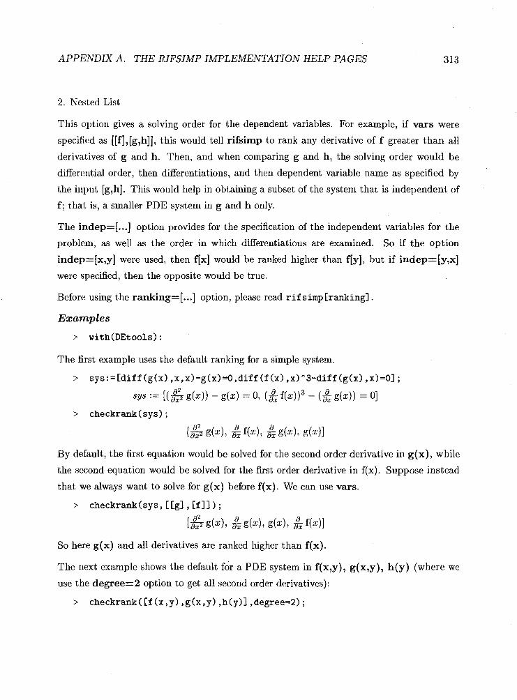
APPENDIX A. THE RIFSIMP IMPLEMENTATION HELP PAGES
2. Nested List
This option gives a solving order for the dependent variables. For example, if vars were
specified as [[f],[g,h]], this would tell rifsimp to rank any derivative of f greater than all
derivatives of g and h. Then, and when comparing g and h, the solving order would be
differential order, then differentiations, and then dependent variable name as specified by
the ix~put [g,h]. This would help in obtaining a subset of the system that is independent of
f ; that is, a smaller PDE system in g and h only.
The indep=[ ...I option provides for the specification of the independent variables for the
problem, as well as the order in which differentiations are examined. So if the option
indep=[x,y] were used, then fCx] would be ranked higher than qy], but if indep=[y,x]
were specified, then the opposite would be true.
Before using the ranking=[ ...I option, please read rif simp Cranking].
Examples
> with(DEtoo1s) :
By default, the first equation would be solved for the second order derivative in g(x), while
the second equation would be solved for the first order derivative in f(x). Suppose instead
that we always want to solve for g(x) before f(x). We can use vars.
> checkrank(sys, Cgl , Cf 11 ; a2 a [m g(x), & g(x), g ( 4 , & f(x)l
So here g(x) and all derivatives are ranked higher than f(x).
The next example shows the default for a PDE system in f(x,y), g(x,y), h (y) (where we
use the degree=2 option to get all second order derivatives):
> checkrank( Cf (x,y) ,g(x,y) ,h(y)l ,degree=2) ;

APPENDIX A. THE RIFSIMP IMPLEMENTATION HELP PAGES
a" a2 a2 a2 a2 a* a2 [G f(x, Y). E(X, Y ) , f(x, Y), rn Y), &z f(x, Y), a;l g(x, Y), &T h(Y), i ) ;i;f(x, Y), &(x, Y), #, f(x, Y), 6 g(l.7 Y)? #, h(Y), f(x, Y) , Y) , h(Y)l
All sctcond order derivatives are first (first 7 entries), then the first derivatives with respect
to x ahead of the first derivatives with respect to y, and finally f(x,y), then g(x,y), then
h(y).
Suppose we want to eliminate higher derivatives involving y before x. We can use indep
for this as follows:
> checkrank( Cf (x,y) ,g(x,y) ,h(y)l, indep=Cy,xl ,degree=2) ;

APPENDIX A. THE RIFSIMP IMPLEMENTATION HELP PAGES 315
A.15 rifread - load intermediate computation as saved using
the 'store' options of rifsimp
Calling Sequences
rifread (filename)
Parameters
filcname - (optional) name of the file containing the partial rifsimp computation.
Description
The rifread command loads a partial rifsimp computation that was run using the store
or storeall options (see rif simp [adv-options] ).
The storage options are most useful for large or complex computations, where the resources
required to complete the computation may exceed the capability of the machine. The state
of thc system at the last iteration (using store), or at all previous iterations and/or cases
(using storeall), can be retrieved using this command.
When called with no arguments, the file "RifStorage.m" is used. This is the default file
name for use with the store option of rifsimp. If a file name was specified for the rifsimp
run, or if the storeall option was used (storing all iterations and/or cases in separate files),
the file name must be included in the rifread command.
Please note that the system obtained using rifread is not in final form and may have
redundant equations or unresolved integrability conditions.
Examples
> with(DEtoo1s) :
Consider the following system, run with rifsimp. > sysi := [diff (xi(x,y) ,y,y),
> diff (eta(x,y) ,y,y)-2*diff (xi(x,y) ,x,y),
> -3*yA2*dif f (xi (x ,y) ,y)+2*diff (eta(x, y) ,x,y)-diff (xi (x, y) ,x,x) ,
> -2*eta(x,y)*y-2*yA2*diff(xi(x,y),x)
> +yA2*diff (eta(x,y) ,y)+diff (eta(x,y) ,x,x)l;

APPENDIX A. THE RIFSIMP IMPLEMENTATION HELP PAGES
ansl := table([ Solved =
I) Partial results can be obtained using rifread, even if the full computation did not succeed
(noticc the presence of the redundant equation et a[yy] =0) .
> tempi := rifreado;
templ := table([
I) Note that the results obtained above were stored in the file "RifStorage.m7'.
The same example can have results stored under a different name. Here the temp results
are stored in " tmpstore.mV :
and := table([ Solved =
I ) > templ := rifread("tmpstoreU);

APPENDIX A. THE RIFSIMP IMPLEMENTATION HELP PAGES
It is also possible to store the results at the end of each iteration and for each separate case
using storeall. Increasing the infolevel will display the file name as each partial calculation
is savod. > sys2 := [-diff (xi (x, y) ,y) *y-diff (xi (x ,y) , y ,y) *yA2,
> +2*diff(eta(x,y),x,y)*yA2+eta(x,y)-diff(xi(x,y),x)*y
> +dif f (xi (x, y) , x) *a*y"2+3*yA3*dif f (xi (x, y) , y) *aA2
> -3*yA4*dif f (xi (x, y) , y) *b^2-3*yA5*diff (xi (x , y) , y) *bA2
> +3*~^2*diff(xi(x,y),y)*a^2,
> diff (eta(x,y) ,x,x)*y^2+yA2*dif f (eta(x,y) ,x)*a
> -y*diff (eta(x,y) ,x)+2*yA3*diff (xi (x,y) ,x) *ae2
> +2*yA2*dif f (xi (x, y) , x) *aA2+yA5*dif f (eta(x, y) , y) *bA2] ;

APPENDIX A. THE RIFSIMP IMPLEMENTATION HELP PAGES 318
i n f ~ l e v e l , ~ ~ ~ , ~ := 1
> rr:=rif simp(sys2, [xi ,eta1 ,storeall,casesp~it) ;
Warning, the following denominator was added to ineqns:
1
The system has been identified as follows :
The system has the following dependent variables :
E , 77
The system has the following independent variables :
x, Y The system has the following constants :
a , b
The following are to be treated as solve variables :
Storing current system in RifStorage-1-1.m Storing current system in RifStorage-I-2.m Storing current system in RifStorage-I-3.m Storing current system in RifStorage-I-4.m Storing current system in RifStorage-I-5.m Storing current system in RifStorage-I-6.m Storing current system in RifStorage-1-7.m Storing current system in RifStorage-I-8.m Storing current system in RifStorage-1-9.m Storing current system in RifStorage-I-1O.m

APPENDIX A. THE RIFSIMP IMPLEMENTATION HELP PAGES
Storing current system in
Storing current system in
Storing current system in
Storing current system in
Storing current system in
Storing current system in
Storing current system in
Storing current system in
Storing current system in
Storing current system in
Storing current system in
a n. := table([l = table([Solved = [& [ ( x , y) = 0, & [ ( a , y) = 0, q ( x , y) = 01,
case = [[b # 0, rl(x7 Y>Il, Pivots = [b # 01
a a ]), 2 = table([Solved = [z [ ( x , y) = 0, z [ ( x , y) = 0, q ( x , y) = 0, b = 01,
case = [[b = 0, rib, Y ) ] , [a ( a - 1) # 0, rl(", Y>l l , Pivots = [a # 0, a - 1 # 01
a a ] ) , 3 = table([Solved = [z [(I, y) = 0, % [ ( I , y) = 0, q ( x , y) = 0, a = 1, b = 01,
case = [[b = 0, q ( x , Y ) ] , [a ( a - 1) = 0, rib, Y ) ] , [a # 0, rl(x, Y>11 I ) , 4 = table([Solved = [
a a ~ ( x , Y ) table([Solved = [% E(x, y) = 0, b = 0, z [ ( x , y) = -, Y
DiflConstraint = [0 = q ( x , y) a ( a - I), 0 = q(x , y) a (a - I ) , 0 = q(x , y) a (a - I),
O = q ( x , y ) a ( 9 a 3 y + 4 y a - 9 y a 2 - 2 a + 2 ) ]
I > A description o f the meaning o f each entry appearing in the output tables can be found on
the rif simp [outputl. page.

Bibliography
[I] A. AHO, J. HOPCROFT, AND J. ULLMAN, Data Structures and Algorithms, Addison-
Wesley, 1983.
[2] T. BECKER, V. WEISPFENNING, AND H. KREDEL, Grobner Bases: A Computa-
tional Approach to Commutative Algebra, vol. 141 of Graduate Texts in Mathematics,
Springer, 1993.
[3] G. W. BLUMAN AND S. KUMEI, Symmetries and Diflerential equations, vol. 81 of
Applied Mathematical Sciences, Springer, 1989.
[4] A. BOCHAROV AND M. BRONSTEIN, Eficiently implementing two methods of the geo-
metrical theory of diflerential equations, Acta. Appl. Math., 16 (1989), pp. 143-166.
[5] F. BOULIER, Some improvements of a lemma of Rosenfeld. Preprint, 1998.
[6] F. BOULIER, D. LAZARD, F. OLLIVIER, AND M. PETITOT, Representation for the
radical of a finitely generated diflerential ideal, in Proc. ISSAC 1995, ACM Press, 1995,
pp. 158-166.
[7] F. BOULIER, F. LEMAIRE, AND M. MAZA, Pardi!, in Proc. ISSAC 2001, ACM Press,
2001, pp. 38-47.
[8] W . BROWN, On Euclid's Algorithm and the Computation of Polynomial Greatest Com-
mon Divisors, J. of the ACM, 18 (1971), pp. 476-504.
[9] B. BUCHBERGER, An Algorithm for Finding a Basis for the Residue Class Ring of a
Zero-Dimensional Polynomial Ideal, PhD thesis, Univ. of Innsbruck, Math. Inst., 1965.

[lo] - , Grobner Bases: An algorithmic method in ideal theory, in Multidi-
n~ensional Systems Theory, D. Reidel Publ. Company, 1985, pp. 184-232.
[ll] G. CARRA FERRO, Grobner bases and diflerential ideals, in Proc. AAECC5, Menorca,
Spain, Springer, 1987, pp. 129-140.
[12] G . CARRA FERRO AND W. SIT, On term-orderings and rankings, in Computational
Algebra, vol. 151 of Lecture Notes in Pure and Applied Mathematics, Marcel Dekker,
1994, pp. 31-77.
[13] E. CARTAN, Sur la structure des groupes infinis de transformations, in Oeuvres
Complhtes Part 11, vol. 2, Gauthier-Villars, 1904, pp. 571-714.
[14] Y . CHEN AND X. GAO, Involutive characteristic sets of algebraic partial diflerential
equation systems, Science in China: Series A, 46 (2003), pp. 469-487.
[15] S. C. CHOU, Mechanical Geometry Theorem Proving, Reidel, 1988.
[16] C. COLLINS, Complex Potential Equations I, Math. Proc. Cambridge Philos. Soc., 80
(1976), pp. 165-187.
[17] T . CORMEN, C. LEISERSON, AND R. RIVEST, Introduction to Algorithms, MIT Press,
1990.
[18] D. Cox, J. LITTLE, AND D. O'SHEA, Ideals, Varieties, and Algorithms, Undergrad-
uate Texts in Mathematics, Springer, 1992.
[19] K. GEDDES, S. CZAPOR, AND G. LABAHN, Algorithms for Computer Algebra, Kluwer,
1992.
[20] V. GERDT, Grobner bases and involutive methods for algebraic and diflerential equa-
tions, in Comp. Alg. in Sci. and Eng., J. Fleischer, J. Grabmeier, F. Hehl, and
W. Kiichlin, eds., World Sci., 1995, pp. 117-137.
[21] V. GERDT AND A. ZHARKOV, Computer generation of necessary integrability condi-
tions for polynomial-nonlinear evolution systems, in Proc. ISSAC 1990, ACM Press,
1990, pp. 250-254.
[22] H. GOLDSCHMIDT, Integrability criteria for systems of partial diflerential equations, J.
Diff. Geom., 1 (1967), pp. 269-307.
[23] D . HARTLEY AND R. TUCKER, A constructive implementation of the Cartan-Kahler
theory of exterior diflerential systems, J . Symbolic Comp., 12 (1991), pp. 655-667.
[24] W . HEREMAN, Review of symbolic software for the computation of Lie symmetries of
differential equations, Euromath Bull., 1 (1994), pp. 45-79.
[25] M . HICKMAN, Symmetry: A maple package for jet bun-
dle computations and lie symmetry computations. Available a t
h t tp : //www .math. canterbury. ac .nz/-mathmsh/Symmetry .html.
[26] L. HSU AND N . KAMRAN, Classi&cation of second-order ordinary diflerential equations
u.dmitting Lie groups of fibre-preserving symmetries, Proc. Lond. Math. Soc., 58 (1989),
pp. 387-416.
[27] E . HUBERT, Factorization free decomposition algorithms in diflerential algebra, J . Sym-
bolic Comp., 29 (2000), pp. 641-662.
[28] - , Notes on triangular sets and triangulation-decomposition algorithms I: Polyno- mial systems, i n Symbolic and Numerical Scientific Computing, vol. 2630 o f Lecture
Notes in Computer Science, Springer Verlag, 2003, pp. 1-39.
P ~ I - , Notes on triangular sets and triangulation-decomposition algorithms 11: Differ- ential systems, in Symbolic and Numerical Scientific Computing, vol. 2630 o f Lecture
Notes in Computer Science, Springer Verlag, 2003, pp. 40-87.
[30] N . IBRAGIMOV, ed., CRC Handbook of Lie Group Analysis of Diflerential Equations,
vol. I , I I , I I I , CRC Press, Boca Raton, 1994,1995,1996.
[31] M . JANET, Sur les Systimes d'e'quations aux de'rive'es partielles, J . d e Math. ( 8 ) , 3
(1920), pp. 65-151.
[32] E. KALTOFEN A N D W. LEE, Early termination in sparse interpolation algorithms, J.
Symbolic Comp., 36 (2003), pp. 365-400.
[33] E . KALTOFEN AND B . TRAGER, Computing with polynomials given by black boxes for
their evaluations: Greatest common divisors, factorization, separation of numerators
and denominators, J . Symbolic Comp., 9 (1990), pp. 301-320.

[34] D. KNUTH, The Art of Computer Programming: Fundamental Algorithms, vol. 1, Ad-
dison Wesley Longman, 3rd ed., 1997.
[35] - , The Art of Computer Programming: Seminumerical Algorithms, vol. 2, Addison Wesley Longman, 3rd ed., 1997.
[36] E. KOLCHIN, Differential Algebra and Algebraic Groups, Academic Press, 1973.
[37] E. MANSFIELD, Diflerential Grobner Bases, PhD thesis, Univ. of Sydney, 1991.
[38] - , The differential algebra package diflgrob2, Maple Tech., 3 (1998), pp. 33-37.
P91 - , Algorithms for symmetric diflerential systems. Technical Report UKC/IMS/99/35, University of Kent at Canterbury, 1999.
[do] E. MANSFIELD, P. CLARKSON, AND G . REID, Nonclassical reductions of a coupled
nonlinear Schrodinger system, Comp. Phys. Comm., 115 (1998), pp. 460-488.
[dl] A. MIOLA AND D. D. Y. YUN, Computational aspects of Hensel-type univariate poly-
nomial Greatest Common Divisor algorithms, in Proc. EUROSAM '74, ACM Press,
1974, pp. 46-54.
[42] B. MISHRA, Algorithmic Algebra, Texts and Monographs in Computer Science,
Springer-Verlag, 1993.
1431 M. MONAGAN AND A. WITTKOPF, On the design and implementation of Brown's
algorithm over the integers and number fields, in Proc. ISSAC '00, St. Andrews, ACM
Press, 2000, pp. 215-223.
[44] J. MOSES AND D. YUN, The EZ-GCD Algorithm, in Proc. ACM '73, ACM Press,
1973, pp. 159-166.
[45] J. D . MURRAY, Mathematical Biology, Springer-Verlag, 1989.
[46] P. OLVER, Applications of Lie Groups to Diflerential Equations, vol. 107 of Graduate
Texts in Mathematics, Springer, 2nd ed., 1993.
PI - , Equivalence, Invariants, and Symmetry, Graduate Texts in Mathematics, Cam- bridge University Press, 1995.

1481 .I.-F. POMMARET, Systems of Partial Differential Equations and Lie Pseudogroups,
Gordon and Breach, 1978.
[491 - , Partial Diflerential Equations and Group Theory: New Perspectives for Applica- tions, Kluwer, 1994.
1501 G . REID, Algorithms for reducing a system of PDEs to standard form, determining the
dimension of its solution space and calculating its Taylor series solution, European J .
o f Appl. Math., 2 (1991), pp. 293-318.
1511 G . REID, P . L I N , A N D A. WITTKOPF, Differential elimination-completion algorithms
for due and pdae, Studies i n Appl . Maths, 106 (2001), pp. 1-45.
[52] G. REID, I . L I S L E , A. BOULTON, A N D A. WITTKOPF, Algorithmic determination
of commutation relations for Lie symmetry algebras of PDEs, i n Proc. ISSAC '92,
Berkeley, P. Wang , ed., ACM Press, 1992, pp. 63-68.
[53] G . REID A N D A. WITTKOPF, Determination of maximal symmetry groups of classes of
differential equations, i n Proc. ISSAC '2000, S t . Andrews, ACM Press, 2000, pp. 264-
272.
1541 G. REID, A. WITTKOPF, A N D A. BOULTON, Reduction of systems of nonlinear partial
differential equations to simplified involutive forms, European J . o f Appl . Math., 7
(1996), pp. 635-666.
[55] C . RIQUIER, Les systimes d'e'quations aux de'rive'es partielles, Gauthier-Villars, 1910.
[56] J . RITT, Differential Algebra, vol. 33 o f Colloquium Publications, A M S , 1950.
[57] A. ROSENFELD, Specializations i n diflerential algebra, AMS Trans., 90 (1959), pp. 394-
407.
[58] C . RUST, Rankings of Derivatives for Elimination Algorithms and Formal Solvability of
Analytic Partial Differential Equations, PhD thesis, Univ. Chicago, 1998. www-address:
www.cecm.sfu.ca/"rust.
[59] C. RUST A N D G . REID, Rankings of partial derivatives, i n Proc. ISSAC '97, Maui,
W . Kiichlin, ed., ACM Press, 1997, pp. 9-16.

[60] C. RUST, G. REID, AND A. WITTKOPF, Existence and uniqueness theorems for formal
power series solutions of analytic diflerential systems, in Proc. ISSAC '99, Vancouver,
S. Dooley, ed., ACM Press, 1999, pp. 105-112.
[61] J . SCHU, W . SEILER, AND J. CALMET, Algorithmic Methods for Lie Pseudogroups, in
Proc. Modern Group Analysis, N. Ibragimov, M. Torrisi, and A. Valenti, eds., Kluwer,
1993, pp. 337-344.
[62] F. SCHWARZ, Reduction and completion algorithms for partial differential equations, in
Proc. ISSAC '92, Berkeley, P. Wang, ed., ACM Press, 1992, pp. 49-56.
[63] -, Janet Bases of 2nd Order Differential Equations, in Proc. ISSAC '96, Zurich,
Y. N. Lakshman, ed., ACM Press, 1996, pp. 179-188.
1641 W. SEILER, Analysis and Application of the Formal Theory of Partial Diflerential
Equations, PhD thesis, Lancaster University, 1994.
[65] -, Applying AXIOM to Partial Diflerential Equations. Technical Report #17, Uni-
versitat Karlsruhe: Institut fiir Algorithmen und Kognitive Systeme, 1995.
[66] C. SULEM AND P . L. SULEM, The Nonlinear Schrodinger Equation, Self-Focussing
and Wave Collapse, vol. 139 of Applied Mathematical Sciences, Springer, 1999.
[67] V. TALANOV, Focusing of light in cubic media, JETP Lett, 11 (1970), pp. 199-201.
[68] A. TRESSE, Sur les invariants difle'rentiels des groupes continus de transformations,
Acta Math., 18 (1894), pp. 1-88.
[69] E. VARLEY AND B. SEYMOUR, Exact solutions for large amplitude waves in dispersive
and dissipative systems, Studies in Applied Math., 72 (1985), pp. 241-262.
[70] D. WANG, Elimination Methods, Springer-Verlag, 2001.
[71] P . S. WANG, The EEZ-GCD algorithm, ACM SIGSAM Bull., 14 (1980), pp. 50-60.
[72] A. WITTKOPF AND G . REID, Benchmark problems for dgerential elimination algo-
rithms. Available at h t t p : //www . cecm. s f u . ca/"wittkopf/systems . h t m l , 2000.
[73] -, Fast differential elimination algorithms. Technical Report TR-00-06, Ontario
Research Centre for Computer Algebra, 2000.
325

[741 - , Fast differential elimination in C: The CDiflElim environment, Comp. Phys.
Comm., 139 (2001), pp. 192-217.
[75] T . WOLF, A package for the analytic investigation and exact solutions of differential
equations, in Proc. EUROCAL '87, vol. 378, Springer, 1987, pp. 479-491.
[76] W . Wu , Basic principles of mechanical theorem proving in elementary geometries, J.
Syst. Sci. Math. Sci., 4 (1984), pp. 207-235.
[771 - , Mechanical Theorem Proving In Geometries: Basic Principles, Springer-Verlag, 1994. translated by Xiaofan Jin And Dongming Wang.
1781 R.. Z IPPEL, Probabilistic Algorithms for Sparse Polynomials, PhD thesis, Massachusetts
Inst. o f Technology, 1979.
PI - , Interpolating polynomials from their values, J . Symbolic Comp., 9 (1990), pp. 375-403.
[go] - , Efective Polynomial Computation, Kluwer, 1993.
[81] W. ZULEHNER AND W . F . AMES, Group Analysis of a semilinear vector digusion
equation, Nonlinear Analysis Theory Methods and Applications, 7 (1983), pp. 945-969.