Algorithms and Criteria for Volumetric Centroidal Voronoi

HAL Id: tel-01455701https://tel.archives-ouvertes.fr/tel-01455701v3

Submitted on 12 Jan 2018

HAL is a multi-disciplinary open accessarchive for the deposit and dissemination of sci-entific research documents, whether they are pub-lished or not. The documents may come fromteaching and research institutions in France orabroad, or from public or private research centers.

L’archive ouverte pluridisciplinaire HAL, estdestinée au dépôt et à la diffusion de documentsscientifiques de niveau recherche, publiés ou non,émanant des établissements d’enseignement et derecherche français ou étrangers, des laboratoirespublics ou privés.

Algorithms and Criteria for Volumetric CentroidalVoronoi Tessellations

Li Wang

To cite this version:Li Wang. Algorithms and Criteria for Volumetric Centroidal Voronoi Tessellations. General Math-ematics [math.GM]. Université Grenoble Alpes, 2017. English. NNT : 2017GREAM002. tel-01455701v3

https://tel.archives-ouvertes.fr/tel-01455701v3

https://hal.archives-ouvertes.fr

THÈSEPour obtenir le grade de

DOCTEUR DE LA COMMUNAUTÉ UNIVERSITÉ GRENOBLE ALPESSpécialité : Mathématiques et InformatiqueArrêté ministériel : 25 mai 2016

Présentée par

Li WANG

Thèse dirigée par Edmond BOYER, INRIA

préparée au sein du Laboratoire Laboratoire Jean Kuntzmann dans l'École Doctorale Mathématiques, Sciences et technologies de l'information, Informatique

Algorithmes et Critères pour les Tessellations Volumétriques de Voronoi Centroïdales

Algorithms and Criteria for Volumetric Centroidal Voronoi Tessellations

Thèse soutenue publiquement le 27 janvier 2017,devant le jury composé de :

Monsieur EDMOND BOYERDIRECTEUR DE RECHERCHE, INRIA DELEGATION ALPES, Directeur de thèseMonsieur FRANCK HETROY-WHEELERMAITRE DE CONFERENCES, GRENOBLE INP, Examinateur Monsieur PIERRE ALLIEZDIRECTEUR DE RECHERCHE, INRIA CENTRE S. ANTIPOLIS - MEDITERRANEE, RapporteurMonsieur BRUNO LEVYDIRECTEUR DE RECHERCHE, INRIA CENTRE NANCY GRAND EST, RapporteurMadame STEFANIE HAHMANNPROFESSEUR, GRENOBLE INP, PrésidentMonsieur SEBASTIEN VALETTECHARGE DE RECHERCHE, CNRS DELEGATION RHONE AUVERGNE, Examinateur

i

Abstract

This thesis addresses the problem of computing volumetric tessellationsof three-dimensional shapes, i.e ., given a three-dimensional shape that isusually represented by its boundary surface, how to optimally subdivide theinterior of the surface into smaller shapes, called cells, according to severalcriteria related to accuracy, uniformity and regularity. We consider centroidalVoronoi tessellations, which are uniform and regular volumetric tessellations.

A centroidal Voronoi tessellation (CVT) of a shape can be viewed as an opti-mal subdivision in the sense that the cells’ centers of mass, called centroids,are regularly distributed inside the shape. CVTs have been used in computervision and graphics because of their properties of uniformity and regularitythat are immune to shape variations. However, problems such as how toevaluate the regularity of a CVT and how to build a CVT from differentrepresentations of shapes remain.

As one contribution of this thesis, we propose regularity criteria basedon the normalized second order moments of the cells. These regularitycriteria allow evaluating volumetric tessellations and specially comparingthe regularity of different Tessellations without the assumption that theirshape and number of sites should be the same. Meanwhile, we proposea hierarchical approach based on a subdivision scheme that preserves cellregularity and the local optimality of CVTs. Experimental results showthat our approach performs more efficiently and builds more regular CVTsaccording to the regularity criteria than state-of-the-art methods.

Another contribution is a novel CVT algorithm for implicit shapes and anextensive comparison between the Marching Cubes, the Delaunay refinementtechnique and our algorithm. The keys of our algorithm are to use convexhulls and local improvements to build accurate boundary cells. We presenta comparison of these three algorithms with different criteria includingaccuracy, regularity and complexity on a large number of different data. Theresults show that our algorithm builds more accurate and regular volumetrictessellations than the other approaches.

We also explore applications such as a shape animation framework basedon CVTs that generates plausible animations with real dynamics.Keywords. Volumetric tessellation • Centroidal Voronoi tessellation • Reg-ularity

iii

Resume

Cette these traite du probleme du calcul d’une tessellation volumiqued’une forme tridimensionnelle, c’est-a-dire, etant donnee une forme tridimen-sionnelle qui est habituellement representee par sa surface frontiere, com-ment subdiviser de maniere optimale l’interieur de la surface en formes pluspetites, appelees cellules, selon plusieurs criteres concernant la precision, l’uni-formite et la regularite. Nous considerons les tessellations de Voronoı cen-troidales qui sont des tessellations volumiques uniformes et regulieres.

Une tessellation de Voronoi centroıdale (CVT) d’une forme peut etre consi-deree comme une subdivision optimale au sens ou les centres de masse,appeles centroides des cellules, sont repartis de maniere optimale a l’interieurde la forme. CVTs ont ete utilises en vision par ordinateur et en infogra-phie en raison de leurs proprietes d’uniformite et de regularite qui sontindependantes des variations de la forme. Cependant, des problemes restentouverts, comme l’evaluation de la regularite d’une CVT ou la constructiond’une CVT a partir de formes representees de diferentes manieres.

Une contribution de cette these est que nous proposons des criteres deregularite basees sur les moments de second ordre normalises des cellules.Ces criteres de regularite permettent d’evaluer les tessellations volumiques,et surtout de comparer la regularite des differentes Tessellations sans l’hy-pothese que leur forme et leur nombre de sites devraient etre les memes.Nous proposons egalement une approche hierarchique basee sur un schemade subdivision qui preserve la regularite des cellules et l’optimalite localedes CVTs. Les resultats experimentaux montrent que notre approche est plusefficace et construit des CVTs plus regulieres que les methodes de l’etat del’art selon les criteres de regularite.

Une autre contribution est une nouvelle algorithme de calcul de CVTpour les formes implicites et une comparaison approfondie entre le Mar-ching Cubes, la technique du raffinement de Delaunay et notre algorithme.La cle de notre algorithme est d’utiliser des enveloppes convexes et uneamelioration locale pour construire des cellules au bord avec precision. Nouspresentons une comparaison des trois algorithmes avec des criteres differents,comme la precision, la regularite et la complexite sur un grand nombre dedonnees differentes. Les resultats montrent que notre methode construit lestessellations volumiques les plus precises et les plus regulieres.

Nous explorons aussi des applications comme, par exemple, une chaınede traitement d’animation des formes basees sur les CVTs qui genere desanimations plausibles a partir de dynamique reelle.Mots-cles. Tessellation volumique • Tessellation de Voronoi centroidale •Regularite

Contents

Contents iv

List of Figures vi

List of Tables xi

Symbols and Abbreviations xiii

1 Introduction 11.1 Context . . . . . . . . . . . . . . . . . . . . . . . . . . . . . . 11.2 Contributions . . . . . . . . . . . . . . . . . . . . . . . . . . 3

2 Volumetric Tessellation 72.1 Introduction . . . . . . . . . . . . . . . . . . . . . . . . . . . 72.2 Voxel-based Approaches . . . . . . . . . . . . . . . . . . . . 102.3 Delaunay-based Approaches . . . . . . . . . . . . . . . . . . 152.4 Voronoi-based Approaches . . . . . . . . . . . . . . . . . . . 27

3 Regularity of a tessellation 353.1 Introduction . . . . . . . . . . . . . . . . . . . . . . . . . . . 353.2 Dimensionless Second Moment . . . . . . . . . . . . . . . . 383.3 Regularity Criteria . . . . . . . . . . . . . . . . . . . . . . . 393.4 Relation to the CVT Energy Function . . . . . . . . . . . . . 45

4 A Hierarchical Approach for Regular CVTs 494.1 Algorithm . . . . . . . . . . . . . . . . . . . . . . . . . . . . 504.2 Evaluation . . . . . . . . . . . . . . . . . . . . . . . . . . . . 554.3 Discussion . . . . . . . . . . . . . . . . . . . . . . . . . . . . 67

5 Voronoi-based Approximated Volumetric Tessellation 695.1 Context . . . . . . . . . . . . . . . . . . . . . . . . . . . . . . 695.2 Algorithm . . . . . . . . . . . . . . . . . . . . . . . . . . . . 71

iv

CONTENTS v

5.3 Evaluation . . . . . . . . . . . . . . . . . . . . . . . . . . . . 745.4 Conclusion . . . . . . . . . . . . . . . . . . . . . . . . . . . . 81

6 Applications 856.1 Clipped Voronoi Tessellation . . . . . . . . . . . . . . . . . . 856.2 Shape Animation with Combined Captured and Simulated

Dynamics . . . . . . . . . . . . . . . . . . . . . . . . . . . . . 91

7 Conclusion 1137.1 Summary of Contributions . . . . . . . . . . . . . . . . . . . 1137.2 Future Research Perspectives . . . . . . . . . . . . . . . . . 114

Bibliography 117

List of Figures

1.1 (a): A surface. (b): A volumetric tessellation. . . . . . . . . . . 21.2 An animation based on tracking and morphing on CVTs. . . . 3

2.1 An overview of volumetric tessellations. . . . . . . . . . . . . . 82.2 Two-dimensional volumetric tessellations for different input

shape (in red). (a): Approximated case when the input is animplicit surface. (b): Exact case when the input is a mesh. . . . 9

2.3 Two-dimensional volumetric tessellations with different ap-proaches for the same input shape (in red). (a): Voxel-based.(b): Delaunay-based. (c) Voronoi-based, with its associatedsites in blue. . . . . . . . . . . . . . . . . . . . . . . . . . . . . . 10

2.4 Overview of voxel-based approaches in two dimensions. (a):Input shape. (b): Voxelization of the domain containing theshape with cubic cells. (c) Approximated clipping in pink. Theimages are from [Anderson]. . . . . . . . . . . . . . . . . . . . . 11

2.5 The 14 basic intersection topologies. Vertices are marked inblack. The intersections between the implicit surface and theedges of cubes and their connections are in red. . . . . . . . . . 13

2.6 The pipeline of general Delaunay triangulation computation. . 162.7 (a, d): The RDT of an implicit surface representing an elephant.

(b, e): The result of (a) after Delaunay refinement. (c, f): Theresult of (b) after a Lloyd optimization. . . . . . . . . . . . . . . 22

2.8 (a): The input shape with the sampling points on its implicitsurface. (b): The RDT. The center of the circumcircle of thetriangles is in blue. The images are from [CGAL]. . . . . . . . . 23

2.9 Overview of the exact Delaunay-based volumetric tessellation.(a): Input shape represented by a mesh. (b): The Delaunaytriangulation of the vertices of the input mesh. (c): The CDTwith the constraints defined by the edges and the facets of themesh. (d): Result after the Delaunay refinement. The imagesare from [Si, 2015]. . . . . . . . . . . . . . . . . . . . . . . . . . . 26

vi

List of Figures vii

2.10 Overview of the computation of a Voronoi-based tessellation intwo dimensions. (a): Initialization: sample the sites inside theinput shape. (b): Voronoi tessellation of the sites. (c): Clipping:compute the clipped Voronoi tessellation. (d): Optimization:update the position of the sites by minimizing the CVT energyfunction. . . . . . . . . . . . . . . . . . . . . . . . . . . . . . . . 28

2.11 (a, c): Voronoi tessellation of sites randomly placed inside theshape. (b, d): The CVT after the optimization. . . . . . . . . . . 32

3.1 Applications of regular volumetric tessellations. . . . . . . . . 36

3.2 Examples of the vertex figure (colored in blue) at a vertex(colored in red) of a pentagon and a cube. . . . . . . . . . . . . 37

3.3 Examples of regular polygons and regular polyhedra. Theimages are from [STUDYBLUE]. . . . . . . . . . . . . . . . . . 37

3.4 Cell of a body-centered cubic lattice. . . . . . . . . . . . . . . . 41

3.5 Voronoi tessellation of a body-centered cubic lattice. The im-ages are from [Blatov et al., 2004]. . . . . . . . . . . . . . . . . . 41

3.6 Example of different tessellations in 2D. The cell regularitymeasure G2(Ωi) is color-coded from blue (regular) to red (farfrom regular). . . . . . . . . . . . . . . . . . . . . . . . . . . . . 43

3.7 Example of a tessellation in 3D with its histogram of cell reg-ularity. (a) Input sphere. (b) A cut of the tessellation. (c)Histogram of its cells regularity. . . . . . . . . . . . . . . . . . 44

3.8 Results of Algorithm 1 in 2D (square with 1000 sites). (a)Error(X) = 0.2. (b) Error(X) = 0.05. (c) Error(X) = 0.02.The cell regularity measure G2(Ωi) is color-coded from blue(regular) to red (far from regular). . . . . . . . . . . . . . . . . . 46

3.9 Results of Algorithm 1 in 3D (sphere with 5000 sites). (a) Inputobject. (b) Error(X) = 0.2. (c) Error(X) = 0.05. (d) Error(X) =0.02. The cell regularity measure G3(Ωi) is color-coded fromblue (regular) to red (far from regular). . . . . . . . . . . . . . . 47

4.1 Overview of our hierarchical approach. . . . . . . . . . . . . . 50

4.2 Subdivision scheme (2D case). (a) Locally optimal CVT: thesites form an hexagonal lattice. (b) Delaunay triangulation ofthe sites. (c) Subdivision: sites are added in the centre of eachedge of the Delaunay triangulation (in red). (d) The new set ofsites also forms an hexagonal lattice. . . . . . . . . . . . . . . . 52

viii List of Figures

4.3 Subdivision scheme (3D case). (a) Delaunay triangulation ofthe sites, which form a BCC lattice. (b) Subdivision: sites areadded in the centre of each edge of the Delaunay triangulation(in blue and purple). The new set of sites also forms a BCClattice. . . . . . . . . . . . . . . . . . . . . . . . . . . . . . . . . . 53

4.4 Hierarchical CVT computation. From an initial CVT with k0 =10 sites (a), successive subdivisions and updates lead to CVTswith k1 = 40, k2 = 160, k3 = 640 and k4 = 2560 sites (from (a)to (e)). The cell regularity measure G(Ωi) is colour-coded fromblue (regular) to red (far from regular). Note how regular areasgrow. . . . . . . . . . . . . . . . . . . . . . . . . . . . . . . . . . 54

4.5 CVTs with 1033 sites. (a) Random sampling + L-BFGS update.(b) Hammersley sampling [Quinn et al., 2012] + L-BFGS update.(c) Global Monte-Carlo [Lu et al., 2012]. (d) Our approach, ran-dom sampling initialization. (e) Our approach, lattice samplinginitialization. (f) Hexagonal lattice. . . . . . . . . . . . . . . . . 58

4.6 (a,c,e,g,i) CVTs with 10025 sites. (b,d,f,h,j) Corresponding reg-ularity histograms: each bin indicates how many cells sharea regularity measure comprised between its boundary values.(a,b) Random sampling + L-BFGS update. (c,d) Hammersleysampling [Quinn et al., 2012] + L-BFGS update. (e,f) Our ap-proach, random sampling initialization. (g,h) Our approach,lattice sampling initialization. (i,j) Hexagonal lattice. . . . . . . 60

4.7 (a,c,e,g) CVTs with 1000 sites in a sphere. (b,d,f,h) CVTs with5000 sites. (a,b) Random sampling + L-BFGS update. (c,d) Ham-mersley sampling [Quinn et al., 2012] + L-BFGS update. (e,f) Ourapproach, random sampling initialization. (g,h) Our approach,lattice sampling initialization. . . . . . . . . . . . . . . . . . . . 62

4.8 Hierarchical CVT computation in 3D. (a) Input: a 3D shapebounded by a triangulated mesh. (b,c,d) Successive CVTscomputed using our approach, with 546, 4375 and 35000 cellsrespectively. (e) A cut of Homer shows that most of the interiorVoronoi cells present high regularity values. . . . . . . . . . . . 64

4.9 More examples of comparaisons between a standard approachand our hierarchical one. From top to bottom: Input shape,Random sampling + L-BFGS update, Our approach with ran-dom sampling initialization, Our approach with lattice initial-ization. . . . . . . . . . . . . . . . . . . . . . . . . . . . . . . . . 65

4.10 Average cell regularity (a) and CVT energy function value (b)with respect to the number of iterations of the CVT update, forthe star shape displayed in Figure 4.6. . . . . . . . . . . . . . . 66

List of Figures ix

5.1 The different steps of the CVT algorithm. The clipping andoptimization steps are iterated until the sites are stabilized. . . 71

5.2 Voronoi tessellations of a torus with and without optimization.(a) A clipped Voronoi tessellation with random initial positionsfor the sites. (b) Clipped CVT after optimization. . . . . . . . . 72

5.3 Tessellations of the characteristic function of a cube: (a) CVT1algorithm without additional points. (b) CVT1 algorithm withsharp feature points added. . . . . . . . . . . . . . . . . . . . . 74

5.4 Accuracy (left), cell regularity (middle) and tetrahedron quality(right) of 3D implicit form tessellations with MC, Delaunayrefinement (Del) and CVT1. . . . . . . . . . . . . . . . . . . . . 80

5.5 The Gargoyle multi-view point cloud and the associated Pois-son reconstructions with Marching Cubes and CVT. Distancesto the implicit form are color encoded on the right, from low(blue) to high (red). . . . . . . . . . . . . . . . . . . . . . . . . . 80

5.6 SKULL: Input point cloud (left) and cell regularity for MarchingCubes and CVT1. . . . . . . . . . . . . . . . . . . . . . . . . . . 81

5.7 Accuracy rankings on 100 meshes from the Princeton Bench-mark [Chen et al., 2009]. Implicit forms were obtained usingPoisson reconstructions [CGAL] and accuracies measured onsamples obtained using the particle system approach [Bergeret al., 2013]. . . . . . . . . . . . . . . . . . . . . . . . . . . . . . . 84

6.1 Different intersection cases. Constraints (line segments) areshown in red. (a, b) Case 1. (c, d, e) Case 2. (f, g, h) Case 3. (i, j)Case 4. (b,e,h) represent singularities. . . . . . . . . . . . . . . 87

6.2 Clipping algorithm. (a) Input: a Voronoi cell and a 3D shape(here: a closed ball) bounded by a mesh. (b) ConstrainedDelaunay triangulations of the boundary of the cell and of themesh. (c) In green: boundary of the cell inside the closed ball.(d) In blue: part of the mesh inside the cell. (e) Result: theclipped cell is bounded by the green and the blue triangulations. 89

6.3 More examples of clipped (non Centroidal) Voronoi diagrams.Left: input triangulations. Right: clipped Voronoi diagrams. . 90

x List of Figures

6.4 From video-based shape capture to physic simulation. (a)Original videos. (b) Volumetric shape representations. (c) Vol-umetric shape tracking (template in blue). (d) Physics-basedsimulation. The approach uses multiple videos and Voronoitessellations to capture the volumetric kinematic of a shapemotion which can then be reanimated with additional mechan-ical effects, for instance volumetric erosion with gravity in thefigure. . . . . . . . . . . . . . . . . . . . . . . . . . . . . . . . . . 95

6.5 (a, b) Input multi-camera observation and point clouds (65386pts). (c, d) Tessellations generated using voxels [Chernyaev,1995]. (e, f) Tetrahedrisations generated using Delaunay refine-ment [CGAL]. (g, h) Clipped Centroidal Voronoi Tessellations(14455 sites). . . . . . . . . . . . . . . . . . . . . . . . . . . . . . 98

6.6 The template model used to recover the runner sequence mo-tion, with its CVT decomposition cells, and the cell clusters indifferent colors. . . . . . . . . . . . . . . . . . . . . . . . . . . . 100

6.7 An animation that combines video-based shape motion (left)and physical simulation (right). Our method allows to applymechanical effects on captured dynamic shapes and generatestherefore plausible animations with real dynamics. . . . . . . . 105

6.8 Input SLACKLINE Multi-camera observations (left), trackingresult of the SLACKLINE sequence (top) and combination withthe effect of collision with a pendulum (bottom). . . . . . . . . 107

6.9 Time persistence on the RUNNER sequence: a slower copy ofthe shape that erodes over time is generated at regular intervals.109

6.10 Tracking result of the RUNNER and the CAGEBIRDDANCE se-quences (middle) and combination with volumetric morphingwith 5000 cells (bottom). . . . . . . . . . . . . . . . . . . . . . . 110

List of Tables

3.1 Comparison of G(P) for various polyhedra in three dimensions[Conway and Sloane, 1982]. P* means a space-filling polyhedron. 40

3.2 Numerical results corresponding to the tessellations in Figure3.6. . . . . . . . . . . . . . . . . . . . . . . . . . . . . . . . . . . 45

4.1 Number of sites after each subdivision, and number of sitesrandomly inserted in boundary cells. . . . . . . . . . . . . . . . 55

4.2 Regularity criteria described in Section 3.3 for CVTs depictedin Figure 4.4. . . . . . . . . . . . . . . . . . . . . . . . . . . . . . 56

4.3 Regularity criteria for CVTs of a square with 10000 sites gener-ated using our hierarchical approach (random sampling initial-ization) with different number of subdivisions. Thus differentnumbers of initial sites. . . . . . . . . . . . . . . . . . . . . . . . 57

4.4 Regularity criteria measures and CVT energy function valuefor CVTs depicted in Figure 4.5. . . . . . . . . . . . . . . . . . . 59



4.7 Computation times for CVTs of shapes depicted in Figures 4.5,4.6, 4.7 and 4.8. . . . . . . . . . . . . . . . . . . . . . . . . . . . . 67

5.1 Accuracy and regularity results on the datasets. (Dmean,Drmse, Gmax, Gmean) ×10−2. . . . . . . . . . . . . . . . . . . 82

5.2 Mean tetrahedron quality measures over all cells of the tessel-lation (best result in bold). . . . . . . . . . . . . . . . . . . . . . 83

5.3 Mean triangle quality measures over all boundary triangle ofthe tessellation (best result in bold). . . . . . . . . . . . . . . . . 83

5.4 Computational time (s) for each experiment. . . . . . . . . . . 83

6.1 Computation times for clipped Voronoi diagrams. . . . . . . . 91

xi

Symbols and Abbreviations

R real coordinate space

M triangle mesh

S shape surface

V shape volume

X point set

Ω three-dimensional domain

Ωi cell of a volumetric tessellation, i corresponds to the index of thei-th site if the tessellation is Voronoi

G average value of a set of dimensionless second moments

πwi power function for the i-th site of a power diagram with respect to

the weight wi

G median value of a set of dimensionless second moments

Bij bisector of the i-th and the j-th Voronoi cells

Bwij bisector of the i-th and the j-th additively weighted Voronoi cells

di Euclidean distance function for the i-th site of a Voronoi tessellation

dgi general distance function for the i-th site of Voronoi tessellation

dwi weighted distance function for the i-th site of an additively weighted

Voronoi tessellation with respect to the weight wi

E CVT energy function

f scalar function

G(P) dimensionless second moment of a polytope P

G2 lower bound of dimensionless second moment in two dimensions

xiii

xiv List of Tables

G3 lower bound of dimensionless second moment in three dimensions

Gmax max value of a set of dimensionless second moments

Grmse root-mean-square error of a set of dimensionless second moments

P polytope

xi i-th site of a Voronoi tessellation

CDT constrained Delaunay triangulation

CVT centroidal Voronoi tessellation

MC Marching Cubes

RDT restricted Delaunay triangulation

Chapter 1

Introduction

Contents1.1 Context . . . . . . . . . . . . . . . . . . . . . . . . . . . 11.2 Contributions . . . . . . . . . . . . . . . . . . . . . . . . 3

1.1 Context

A shape is usually represented by its boundary surface and is largelyused in computer vision and graphics. However, the information offeredby a shape surface is not always sufficient for several applications [Ravivet al., 2010] [Allain et al., 2016]. In order to cover more information,volumetric data that represents the interior of a shape surface, i.e . the shapevolume, is used. The aim of a volumetric tessellation is to build a volumetricquantization of a shape volume by filling it with small cells as shown inFigure 1.1. A good volumetric tessellation [Wang et al., 2016b] consists ofuniform and regular cells with a good approximation to the boundarysurface. The analysis of the goodness of a volumetric tessellation and theconstruction of a good volumetric tessellation remain a challenge.

A volumetric tessellation can be computed using many approachesthat can be roughly divided into two categories according to the algorithmthey use: Eulerian approaches and Lagrangian approaches. Eulerian ap-proaches consider a grid discretizing the observation domain that containsthe shape. The grid is usually fixed and composed of the same sized cellsthat are identified inside or outside the shape. The volumetric tessel-lation can be further obtained by computing the intersection betweenthe grid and the shape. These approaches are fast. However, a largewaste of memory occurs when the observation domain is relatively large

1

2 CHAPTER 1. INTRODUCTION

(a) (b)

Figure 1.1 – (a): A surface. (b): A volumetric tessellation.

compared to the shape and irregular cells are often generated on theboundary. Instead of discretizing the observation domain containingthe shape, Lagrangian approaches discretize directly the shape that re-duces the complexity. These approaches usually include an optimizationphase that provides the goodness control of the generated volumetrictessellations.

Centroidal Voronoi tessellation (CVT) is a Lagrangian approach thatis widely used in many applications due to its good properties. Anexample is shown in Figure 1.2. The CVT algorithm distributes points,called sites, inside the shape and computes the intersection between theVoronoi tessellation of the sites and the shape. Then the site positions areupdated by minimizing the so-called CVT energy function that measuresthe quantification error. The final volumetric tessellation consists of thecells centered around the sites. A CVT corresponds to a local minimum ofits energy function. However, finding the optimal CVT that correspondsto the global minimum of its energy function remains a challenge sincethe energy function is usually non-linear and non-convex.

This thesis focuses on the construction of CVTs and their analysisincluding an evaluation and comparison with other existing approaches.

1.2. CONTRIBUTIONS 3

Figure 1.2 – An animation based on tracking and morphing on CVTs.

It attempts to answer the following questions: 1. How can the regularity bedefined for a volumetric tessellation ? 2. How to generate a CVT as closeto the optimal as possible ? 3. How to compare different approaches tocompute volumetric tessellations ? 4. What are possible new applicationsof regular volumetric tessellations ? The answers are detailed in Chapters3, 4, 5 and 6, respectively.

1.2 Contributions

The main contributions of this thesis are detailed into Chapters 3, 4, 5and 6. Before entering these chapters, the state of the art for volumetrictessellation approaches is reviewed in Chapter 2. Finally, the conclusionsand future work are presented in Chapter 7.

Chapter 3

In this chapter, we build on a theoretical work of Conway and Sloane[1982] and propose regularity criteria for volumetric tessellations. Thesecriteria are based on the normalized second order moments of polyhedra.We show that the regularity criteria are linked to the CVT energy functionbut are dimensionless and therefore enable global evaluations as well ascomparisons. We also propose an application of one of these criteria byconsidering it as the stopping criterion for CVT computation. This workhas been published in [Wang et al., 2016a];

Chapter 4

In this chapter, we propose a hierarchical approach that provides CVTswith more regularity than state-of-the-art methods. Our strategy is based

4 CHAPTER 1. INTRODUCTION

on a subdivision scheme that preserves cell regularity and the local opti-mality of CVTs on unbounded domains. This scheme tends to propagatecell regularity through hierarchy levels when applied to bounded do-mains. We demonstrate the efficiency of this framework with an in-depthevaluation that includes sensitivity analysis, comparisons with previouswork and analyses of the convergence speed and computation time. Thiswork has been published in [Wang et al., 2016a];

Chapter 5

In this chapter, we propose a novel approach that builds CVTs fromimplicit forms. These tessellations provide volumetric and surface repre-sentations with strong regularities in addition to provably more accurateapproximations of the implicit forms considered. In order to comparewith other existing approaches, we present an extensive evaluation thatanalyzes various properties of the main approaches for implicit to explicitvolumetric tessellations: Marching Cubes, Delaunay refinement and CVTs,including accuracy and shape quality of the resulting shape mesh. Thiswork has been published in [Wang et al., 2016b].

Chapter 6

In this chapter, we propose a novel polyhedra clipping algorithm tocompute clipped Voronoi tessellations. This algorithm reduces the three-dimensional clipping problem to a two-dimensional triangle-triangle in-tersection problem. We demonstrate the efficiency and robustness ofour algorithm with a wild range of experiences. This work has beenpublished in [Wang et al., 2016a]. We also propose a novel system foranimation generation. This system first generates CVTs from a stream ofthree-dimensional observations acquired with a video-based capture sys-tem, then produces animation by combining video-based shape motionand mechanical effects on the generated CVTs. This work has been madeavailable in [Allain et al., 2016].

List of Publications

• Li Wang, Franck Hetroy-Wheeler, Edmond Boyer. A HierarchicalApproach for Regular Centroidal Voronoi Tessellations. In ComputerGraphics Forum 2016 (Vol. 35, No. 1, pp. 152-165).• Li Wang, Franck Hetroy-Wheeler, Edmond Boyer. On Volumetric

Shape Reconstruction from Implicit Forms. In ECCV 2016 - European

1.2. CONTRIBUTIONS 5

Conference on Computer Vision, Oct 2016, Amsterdam, The Nether-lands.

• Benjamin Allain, Li Wang, Jean-Sebastien Franco, Franck Hetroy-Wheeler, Edmond Boyer. Shape Animation with Combined Cap-tured and Simulated Dynamics. In arXiv:1601.01232, ArXiv. 2016.

Chapter 2

Volumetric Tessellation

Contents2.1 Introduction . . . . . . . . . . . . . . . . . . . . . . . . . 72.2 Voxel-based Approaches . . . . . . . . . . . . . . . . . 102.3 Delaunay-based Approaches . . . . . . . . . . . . . . . 152.4 Voronoi-based Approaches . . . . . . . . . . . . . . . . 27

2.1 Introduction

A volumetric tessellation of a shape volume V consists of one or moresmaller shapes that fill V with no overlap and no gap. It is also calledtilling, partition or subdivision of V . These smaller shapes of the volu-metric tessellation are called cells and noted the Ωi. A shape is usuallyrepresented by its boundary that is a surface S . It has to be mentionedthat volumetric tessellations are different from surface tessellations thatare restricted to S . Volumetric tessellations can be generalized to anydimensions. In this thesis, we focus on tessellations in three dimensions.

Over the last decade, the construction of volumetric tessellations hasbeen largely studied and used for applications in both computer visionand computer graphics. Many methods have been proposed for differ-ent applications. Depending on the input, the methods can be roughlydivided into two categories. When the input is an implicit representationthat identifies a shape volume V as being a region within an observationdomain Ω, the output tessellation is an approximation of V [Lorensen andCline, 1987] [Jamin et al., 2015]. Such implicit representation is typicallygiven as a scalar function f : Ω → R that takes different values inside

7

8 CHAPTER 2. VOLUMETRIC TESSELLATION

Figure 2.1 – An overview of volumetric tessellations.

and outside V , for instance an implicit function, an indicator function ora distance function. This implicit representation can be characterized byan implicit surface that is usually obtained for a real object through sur-face reconstruction methods from point clouds [Berger et al., 2014]. Theconversion from implicit surfaces to explicit volumetric tessellations isalso called polyhedrization or mesh generation [Jamin et al., 2015]. Whenthe input is an explicit representation, usually a polygonal meshM, theoutput tessellation is exact with its associated polygonal surface that isidentical toM [Yan et al., 2013] [Si, 2015]. Without specification,M refersto a triangle mesh in this thesis. Figure 2.2 gives an illustration of thedifference between the two cases in two dimensions.

2.1. INTRODUCTION 9

(a) (b)

Figure 2.2 – Two-dimensional volumetric tessellations for different inputshape (in red). (a): Approximated case when the input is an implicitsurface. (b): Exact case when the input is a mesh.

Depending on the algorithms they used, the methods can be roughlycategorized into voxel-based, Delaunay-based and Voronoi-based ap-proaches. Voxel-based approaches include the Marching Cubes method[Lorensen and Cline, 1987] and its extensions. They use a fixed gridthat discretizes the observation domain Ω containing the shape volumeV into cells that are usually identical such as cubes or tetrahedra forinstance. Then the intersection between V and the cells is computed.Delaunay-based approaches, such as [Jamin et al., 2015] and [Si, 2015],build a three-dimensional Delaunay triangulation, also called tetrahedral-ization, with the sampling points on the shape surface S . Voronoi-basedapproaches compute the intersection between V and the Voronoi diagram,dual of the Delaunay triangulation, of points xi, called sites, that aresampled inside V. Figure 2.3 visualizes the difference between these threeapproaches with the same input in two dimensions.

Figure 2.1 shows the overview of the volumetric tessellation process.Following this overview, Voxel-based, Delaunay-based and Voronoi-basedapproaches are reviewed in details in Section 2.2, 2.3 and 2.4, respectively.


(a) (b) (c)

Figure 2.3 – Two-dimensional volumetric tessellations with different ap-proaches for the same input shape (in red). (a): Voxel-based. (b): Delaunay-based. (c) Voronoi-based, with its associated sites in blue.

2.2 Voxel-based Approaches

Voxel-based approaches for implicit surfaces include the well-knownMarching Cubes (MC) algorithm and its extensions. It has to be mentionedthat the MC has originally been proposed for the isosurface extractionproblem. Most of the improvements on the MC are designed for require-ments at the surface level, for instance surface simplification. However,since the essential idea of the MC is to use a volumetric grid to discretizethe domain that contains the input shape, it belongs to the set of volu-metric tessellation approaches. Besides, the volumetric output generatedby the MC have been used in many applications. For example, Wu et al.[2015] considered the volumetric output as the input for deep learning ofshape recognition, and Raviv et al. [2010] used it to find volumetric heatkernel signatures of shapes.

The process of voxel-based approaches consists of two main steps asfollows:

1. Voxelization: use a grid to discretize the domain containing theinput shape.

2. Clipping: compute the intersection between the grid and the inputshape.

Figure 2.4 visualizes these steps using an example in two dimensions.The grid used for voxelization is usually fixed and constructed with cubessharing the same size. However, many extensions using grids with cellsof different shapes, such as multi-resolution or tetrahedra, have beendesigned for the purpose of complexity simplification or disambiguation.

2.2. VOXEL-BASED APPROACHES 11

(a) (b) (c)

Figure 2.4 – Overview of voxel-based approaches in two dimensions. (a):Input shape. (b): Voxelization of the domain containing the shape withcubic cells. (c) Approximated clipping in pink. The images are from[Anderson].

These extensions are reviewed in Section 2.2.1. When the input shape is amesh, the clipping step boils down to a polyhedron intersection problembetween the mesh and the cells of the grid. Otherwise, it is the typicalapproximated clipping of the original MC algorithm. Voxel-based ap-proaches are widely used because of their time efficiency. However, thegenerated cells in the boundary can be very irregular and non-uniform.We detail the clipping algorithm that uses cubic grid since it is moreinteresting in terms of regularity than other grids in Section 2.2.2. Redun-dancy, correctness and consistency problems arise when the tessellationis an approximation of an implicit input. Although many solutions havebeen proposed, these problems remain a challenge. Improvements arereviewed in Section 2.2.3.

2.2.1 Voxelization

The voxelization in the original MC algorithm from Lorensen andCline [1987] adopts a fixed grid with the same sized cells which are cubes.This is because cube is one of the simplest space-filling polyhedron and iseasy to construct. However, it causes not only ambiguity problems butalso a waste of memory, especially when the size of cubes is chosen tobe too small compared to the input volume. Many extensions have beenproposed to solve these problems. Depending on the shape of cells, thesemethods can be divided into two categories: multi-resolution cells andnon-rectangular cells.

In order to reduce the memory complexity and to generate triangleswith adaptive size on the shape surface, Shu et al. [1995] considered an


adaptive MC that subdivides the cubes according to the shape surfacesmoothness. This method may cause cracks in the generated surface.Although a crack-patching method is applied for filling the cracks withpolygons of the same shape, loss of finer features may happen whensubdividing the cubes. An octree structure is used in [Shekhar et al., 1996]that replaces small cells with a larger one instead of subdividing. In orderto patch the cracks, edges of the smaller cells are forced to coincide withthose of their larger neighbors. This crack-patching method does notgenerate new triangles. Weber et al. [2003] extended the MC to rectilineargrid with multi-resolution. The cracks among the cells are then filled withpolyhedra.

Instead of using cubes as cells, tetrahedra are firstly considered inan algorithm proposed in [Akio and Koide, 1991] that is called March-ing Tetrahedra. It subdivides each cube cell into four tetrahedra. Theadvantage of using tetrahedra is that it simplifies the lookup table andeliminates the ambiguities of the facetization. However, the complexityincreases and the orientation of each tetrahedron has to be defined. March-ing Tetrahedra has been widely used in many applications and also beenapplied to rectilinear grid and multi-resolution [Elvins, 1992]. Other celltypes such as hexahedron [Carr et al., 2003], octahedron [Carr et al., 2003][Takahashi et al., 2004] and other irregular shapes [Newman and Yi, 2006]have been considered for the purpose of complexity reduction.

These extensions are mainly proposed for improving the generatedsurface quality without considering the regularity of the generated volu-metric tessellation. In the following, we consider the voxelization witha fixed grid with the cubes of the same size because it generates moreregular tessellations compared to the others.

2.2.2 Clipping

Depending on the type of input shapes, the clipping algorithm is eitherapproximated or exact. In the exact case where the input shape is a mesh,the problem becomes a polyhedron intersection problem between themesh and the cells. Sutherland’s clipping algorithm [Sutherland andHodgman, 1974] can be used. In Chapter 6, we introduce a novel, efficientand robust clipping algorithm. This work has been published in [Wanget al., 2016a].

When the input shape is an implicit surface, the standard clippingalgorithm is the MC algorithm. The standard MC algorithm [Lorensenand Cline, 1987] first identifies the boundary cubes that intersect theimplicit surface by marking the vertices inside the shape. There are 256

2.2. VOXEL-BASED APPROACHES 13

[Lopes and Brodlie, 2003]

Figure 2.5 – The 14 basic intersection topologies. Vertices are marked inblack. The intersections between the implicit surface and the edges ofcubes and their connections are in red.


(28) possibilities for a cube since a cube has eight vertices that can beeither marked or unmarked. However, if rotational, reflective and mirrorsymmetries are considered, the intersection topologies can be reducedto only 14, as shown in Figure 2.5. For each topology, the approximatedsurface is generated by connecting the intersections between the implicitsurface and the edges of cube. This information is stored in a look-uptable that makes the process very fast.

The intersection between the implicit surface and the edges can beestimated using an interpolation method. Depending on the informationavailable on the vertices, different methods can be applied. When onlyimplicit function values are available, linear interpolation is widely usedbecause it is fast and simple. The false position method gives better resultsby locating the intersection iteratively. When both implicit function valuesand their derivatives are available, Hermite interpolation is proposed togive an accurate intersection [Fuhrmann et al., 2015]. When no additionalinformation than inside or outside is offered, the bisection method canbe used which can iteratively locates the intersection within a precisiondefined by user.

It has been pointed out that there are ambiguities in the standardMC algorithm [Nielson and Hamann, 1991] [Natarajan, 1994]. In Figure2.5, there are face ambiguities in cases 3, 6, 7, 10, 12 and 13 and interiorambiguities in cases 4, 6, 7, 10, 12 and 13. Chernyaev [1995] identified thatthere are 33 different cases where two of them can be removed because ofreflective and mirror symmetries. Many methods have been proposed fordisambiguation that are reviewed in Section 2.2.3.

2.2.3 Improvements

There are two main issues in approximated volumetric tessellationsusing the standard MC algorithm that are topological inconsistency andnon-manifoldness. The topological inconsistency issue comes from theambiguities in the standard MC cases as firstly noted by Durst [1988].The asymptotic decider method [Nielson and Hamann, 1991] has beenproposed for solving the face ambiguity using bilinear interpolation ofambiguous faces’ vertices. Then the lookup table of the standard MC algo-rithm has been extended to 33 cases [Chernyaev, 1995] by adding subcasesfor disambiguation. An interior discriminant has also been proposed forthe internal ambiguity subcases by detecting bilinear interpolations overany plane inside the ambiguous cubes. Nielson [2003] and Lopes andBrodlie [2003] proposed trilinear interpolation methods that provide an el-

2.3. DELAUNAY-BASED APPROACHES 15

egant solution to both face and internal ambiguities. The implementationfor [Chernyaev, 1995] is available in [Lewiner et al., 2003].

Manifoldness can be lost if the facetization generates non-manifoldedges. Nielson [2003] and Lopes and Brodlie [2003] proposed to generateadditional points on the boundary and inside cube for preserving bothtopological consistency and manifoldness. Etiene et al. [2012] mentionedthat the implementation of [Lewiner et al., 2003] may fail to producemanifold surface. The method has been then improved by Custodio et al.[2013]. Recently, a novel method using quadratic equations is proposedfor generating both topological consistent and manifold surface in [Grosso,2016]. For more detail reviews on this topic, please see [Newman and Yi,2006].

2.3 Delaunay-based Approaches

The main step of Delaunay-based approaches is the Delaunay trian-gulation that fills a shape volume V with three-dimensional triangles,i.e . tetrahedra. The computation of a triangulation of a point set can bedefined as a process of associating the points by forming triangles. Givena finite set of points X , a triangulation of X is a simplicial complex thattessellates the convex hull of X and whose vertices belong to X . Severaltriangulations may be constructed from the same set of points. Amongthem, the Delaunay triangulation is the most interesting one since it pos-sesses good properties. The Delaunay triangulation and its dual, theVoronoi diagram, are widely studied and used in many applications ofdifferent areas. After some extensions such as the constrained Delaunayand the restricted Delaunay triangulations have been proposed, it hasbeen used for volumetric tessellations of shapes, also called volumetricmesh generation.

The remainder of this section is organized as follows: We first intro-duce the background on the Delaunay triangulation of a point set includ-ing its algorithms and extensions in Section 2.3.1. Then the Delaunay-based volumetric tessellations in the approximated case and in the exactcase are reviewed in Section 2.3.2 and Section 2.3.3, respectively.

2.3.1 Background on Delaunay Triangulations

The Delaunay triangulation was first proposed by Delaunay [1934].Given a finite point set X , the Delaunay triangulation of X is the triangu-lation such that each triangle has a circumsphere which does not contain


Figure 2.6 – The pipeline of general Delaunay triangulation computation.


the other points. Among all the triangulations of X , the Delaunay trian-gulation maximizes the smallest angle of the triangles in the triangulation.This means that for the maximum minimum angle criterion, the Delaunaytriangulation is the best one of all the triangulations of X . If all the pointsin X lie on the same line, there is no Delaunay triangulation. If four ormore points are cocyclic, the Delaunay triangulation is not unique.

A Delaunay triangulation can also be defined by higher dimension em-bedding. Given a finite point set X = xi in an m-dimensional Euclideanspace Em, the parabolic lifting map [Brown, 1979] transforms the Delaunaytriangulation of X into a convex hull in Em+1. Each xi ∈ X correspondsto x′i = (xi, ‖xi‖2) ∈ X ′ in Em+1 and the Delaunay triangulation of X isthe projection on the m-dimensional plane of the convex hull of X ′ in Em.

Because of its nice properties [Fortune, 1992] [Loera et al., 2010], the De-launay triangulation is used for graph construction [Chew, 1986], networkoptimization [Mitchell, 2000] etc . Over the last decades, many extensionsof the Delaunay triangulation have been proposed for requirements ofdifferent applications. We use the pipeline of the general Delaunay trian-gulation computation to gather the extensions in a systematic way. Figure2.6 shows the pipeline that consists of a triangulator, a constrained trian-gulator and an optimizer. The triangulator takes a finite point set X asinput and computes the Delaunay triangulation of X . When X consists ofpoints with weights, the weighted Delaunay triangulation or the regulartriangulation methods can be computed. Then the triangulator passesthe triangulation of X to the constrained triangulator which adjusts theinput triangulation according to the given constraints. The constrainedDelaunay triangulation method forces some fixed segments or polygonsto appear in the triangulation and the restricted Delaunay triangulationmethod allows removing all the triangles that are outside the given shape.Since the above process cannot guarantee the triangulation to be Delaunay,the conforming Delaunay triangulation method in the optimizer splitsthe non-Delaunay edges by inserting additional points (Steiner points)and reconstitutes the triangulation until it satisfies the Delaunay criterion.The Delaunay refinement method subdivides the triangulation in order toimprove its quality.

In Section 2.3.1.1, we review the algorithms for basic Delaunay trian-gulation of point sets. The main extensions of the Delaunay triangulationare listed in Section 2.3.1.2.


2.3.1.1 Delaunay Triangulation Algorithms

Algorithms for the three-dimensional Delaunay triangulation can beclassified into the following categories: incremental reconstruction, incre-mental insertion, higher dimensional embedding and divide and conquer.The incremental reconstruction algorithm [Joe, 1991] starts with a singletetrahedron without containing any other of input points. Then inputpoints are inserted successively to the existing Delaunay triangulationand uses local transformations known as the flip algorithm is used tobuild a new Delaunay triangulation. In order to accelerate the algorithm,the input points can be sorted before or stored in a uniform grid [Joe,1991]. Unlike the incremental reconstruction algorithm that inserts pointsoutside the existing triangulation, the incremental insertion algorithminserts points inside it. In order to build a new triangulation, one strategyis to delete the tetrahedra whose circumsphere contains the inserted pointand then to rebuild a triangulation to fill the hole [Bowyer, 1981] [Watson,1981]. Another strategy is to use local transformations [Facello, 1995].As mentioned earlier, the Delaunay triangulation can be defined by theprojection of the convex hull in higher dimension. The input points arefirstly embedded into four dimensions by the lifting map. Then theirconvex hull and its projection in three dimensions are computed to obtainthe Delaunay triangulation [O’Rourke and Goodman, 2004]. A divide andconquer algorithm [Cignoni et al., 1998a] divides the input points intosmall partitions using splitting planes. Then the Delaunay triangulationof each partition is computed. The last step is to merge them to the finalDelaunay triangulation. The parallel versions of some of the above algo-rithms are proposed in [Kohout and Kolingerova, 2003] [Kohout et al.,2005] [Lo, 2012].

2.3.1.2 Extensions of Delaunay Triangulations

In this section, we review the main extensions of the Delaunay trian-gulation. As mentioned earlier, the Delaunay triangulation can be definedin several ways, such as by the requirement that the circumspheres of alltetrahedra in triangulation do not contain other vertices or by the projec-tion of convex hull in higher dimensions using the parabolic lifting map.In order to define the Delaunay triangulation and some of its extensionssuch as the weighted Delaunay triangulation or the regular triangulationin a consistent way, we use the notion of Voronoi diagram, also calledVoronoi tessellation, which is the dual of the Delaunay triangulation.

Given a finite set of n points X = xini=1 in three-dimensional Eu-


clidean space E3, we define a distance function di, also called cost function,for each xi as follows:

di : E3 −→ R

x 7−→ ‖x− xi‖2,(2.1)

where ‖ · ‖ is the Euclidean distance. The Voronoi region Ωi, also calledVoronoi cell, of xi is the set of points that are closest to xi than to any otherpoints of X . That is:

Ωi = x ∈ E3 ‖ di(x) ≤ dj(x), ∀j 6= i. (2.2)

xi is called the site of Ωi. The bisector Bij of two Voronoi cells Ωi andΩj is the set of points that are shared by these two cells. That is

Bij = x ∈ E3 ‖ ‖x− xi‖ = ‖x− xj‖. (2.3)

The Delaunay triangulation of X can be constructed from the Voronoidiagram by connecting two sites whose corresponding Voronoi cells sharea bisector. We use analogous definitions to define weighted Delaunaytriangulation and regular triangulation in the following paragraphs.

Weighted Delaunay Triangulation

Given a finite set of n pointsX = xini=1 ∈ E3 with weights win

i=1 ∈R, we define a distance function dw

i for xi as follows:

dwi : E3 −→ R

x 7−→ ‖x− xi‖ − wi,(2.4)

where ‖ · ‖ is the Euclidean distance. Using this distance function, wecan define an analog to the Voronoi diagram that is called the additivelyweighted Voronoi diagram with its cells defined as follows:

Ωwi = x ∈ E3 ‖ dw

i (x) ≤ dwj (x), ∀j 6= i. (2.5)

The bisector Bwij of two additively weighted Voronoi cells is defined as

follows:

Bwij = x ∈ E3 ‖ ‖x− xi‖ − wi = ‖x− xj‖ − wj. (2.6)

Recall that the weighted Delaunay triangulation of X can be obtainedfrom the additively weighted Voronoi diagram by connecting two siteswhose corresponding cells share a bisector.


Regular Triangulation

Given a finite set of n pointsX = xini=1 ∈ E3 with weights win

i=1 ∈R, we define a distance function πw

i for xi as follows:

πwi : E3 −→ R

x 7−→ ‖x− xi‖2 − wi,(2.7)

where ‖ · ‖ is the Euclidean distance. This function is also called power func-tion and is used to define the power diagram. Then the regular triangulationof X can be defined in the same way as the Delaunay triangulation.

It has to be mentioned that although both the weighted Delaunaytriangulation and the regular triangulation use weighted point sets, theyuse different distance functions. Intuitively, the bisectors of the regulartriangulation are planes. However, the bisectors of the weighted Delaunaytriangulation may be radical planes.

Constrained Delaunay Triangulation

A constrained Delaunay triangulation (CDT) [Chew, 1989] is an ex-tension of the Delaunay triangulation that enforces certain geometricconstraints into the triangulation such as segments and polygons in threedimensions. Usually, the tetrahedra that contain the constraints do notsatisfy the Delaunay triangulation criterion, thus, a CDT is not neces-sarily Delaunay. The computation of CDTs is the main step of the exactDelaunay-based volumetric tessellation. The input mesh is considered asa set of constraints in the tessellation. CDT algorithms are reviewed indetail in Section 2.3.3.1.

Restricted Delaunay Triangulation

A restricted Delaunay triangulation (RDT) is an extension of the De-launay triangulation that forces the triangulation to stay inside the inputshape. In the exact case, only the tetrahedra inside the input mesh arekept. In the approximated case, the center of the circumsphere of thetetrahedron can be used for checking if the tetrahedron is inside the inputimplicit surface [Jamin et al., 2015]. The computation of RDTs is the mainstep of the approximated Delaunay-based volumetric tessellation and isreviewed in detail in Section 2.3.2.2.


Conforming Delaunay Triangulation

A conforming Delaunay triangulation is an extension of the CDT thatsubdivides the constraints by inserting additional points (Steiner points).These points allow to keep the constraints in the triangulation whilesatisfying the Delaunay criterion.

Delaunay Refinement

The Delaunay refinement is an optimization process for the purpose ofimproving the tetrahedra quality by subdividing the edges, facets or cellsin tessellations. However, it also has several drawbacks. The process mayproduce badly shaped tetrahedra and may have non-terminating loopsbecause of sharp features. Different versions of the Delaunay refinementare proposed for both the approximated and the exact cases. See thedetails in Section 2.3.2.3 and 2.3.3.2.

2.3.2 Approximated Case

The computation of an approximated Delaunay-based volumetrictessellation considers a shape volume V as input and builds a RDT insideV . In this case, the input V is usually represented by an implicit surfaceS representing its boundary and the constructed RDT is supposed toapproximate V . The computation consists of the following three steps:

1. Initialization: sample a finite set of points X lying on S . If sharpfeatures are required to be preserved, the points lying on the sharpedges are sampled and inserted into X .

2. RDT: build the RDT of X inside V .

3. Optimization: subdivide edges, faces or cells of the RDT by insertingadditional points (Steiner points) into X or change the position ofthe existing points in X , then rebuild the RDT of the updated Xuntil certain user-defined mesh quality criteria are satisfied.

Figure 2.7 gives an illustration of the results after different steps. Aswe can see, after step 1 and 2, a RDT with badly shaped tetrahedra isconstructed (see Figure 2.7 (a) and (d)). (b) and (e) in Figure 2.7 showthat the triangulation is subdivided by inserting additional points and thenew constructed tetrahedra are better shaped. This subdivision processis called the Delaunay refinement and the additional points are calledSteiner points. The quality of the triangulation can be further improved byupdating the position of the points using variational methods (see Figure


(a) (b) (c)

(d) (e) (f)

Figure 2.7 – (a, d): The RDT of an implicit surface representing an elephant.(b, e): The result of (a) after Delaunay refinement. (c, f): The result of (b)after a Lloyd optimization.

2.7 (c) and (f)). These three steps are reviewed in detail in Section 2.3.2.1,2.3.2.2 and 2.3.2.3, respectively.

2.3.2.1 Initialization and Sharp Features

In order to build a RDT inside the input shape volume V , a finite setof points X is sampled on the implicit surface S during the initializationstep. Several methods can be used for obtaining these initial points suchas random ray shooting for instance. X may be also provided by the user.It is worth mentioning that the uniform distribution and high density ofX can improve the quality of the RDT so that the tetrahedra are moreregular and the triangulation approximates better to V . However, uniform


sampling on S can be difficult when S is complex. Instead of generatingan uniform sampling in the intialization step, the quality of regularityand approximation of the RDT can be improved in the optimization step.During the computation of the Delaunay refinement, the Steiner pointsare inserted inside V or on S according to certain criteria of regularity andapproximation. With the Delaunay refinement, the initialization step canbe simplified to only sample a small set of points on S .

Sharp features can be easily integrated into the Delaunay-based ap-proach during the initialization step. The protecting-balls approach[Cheng et al., 2010] is proposed to ensure that the given sharp featuresappear in the final tessellation. The approach discretizes the sharp fea-tures into a set of weighted points that are called protecting balls. Theseweighted points are then inserted into X and the weighted Delaunaytriangulation is used instead of the Delaunay triangulation in the wholetriangulation process. The points except for the protecting balls have zeroweight so that the sharp edges can be forced into the final triangulation.

2.3.2.2 Restricted Delaunay Triangulation

(a) (b)

Figure 2.8 – (a): The input shape with the sampling points on its implicitsurface. (b): The RDT. The center of the circumcircle of the triangles is inblue. The images are from [CGAL].

The RDT is the main step of the approximated Delaunay-based volu-metric tessellation. It consists of building a Delaunay Triangulation andrestricting this Delaunay triangulation to the input shape volume V . Inorder to remove the tetrahedra outside V , the center of the circumspheres


are used. For each tetrahedron of the Delaunay triangulation, if the centerof its circumsphere is outside V , the tetrahedron is considered as outsideV and has to be removed. Otherwise, the tetrahedron is kept. Figure 2.8gives a two-dimensional illustration of the RDT. It is important to notethat as a result of the process of removing tetrahedra, it is difficult toguarantee the topological consistency and the manifoldness of the finaltessellation and its surface, even with a dense sampling [Oudot, 2008].

2.3.2.3 Optimization

The optimization step aims at building a good tessellation that ap-proximates well the input shape volume V and is composed of regulartetrahedra. As mentioned earlier, it is difficult to obtain a uniform anddense sampling on the implicit surface S during the initialization step.With only the sampling points lying on S , the RDT contains badly shapedtetrahedra (see Figure 2.7 (a) and (d)). The Delaunay refinement subdi-vides facets and cells of the triangulation by inserting Steiner points insideV and on S . Variational methods and local optimization allow removingdegenerate tetrahedra called slivers. Slivers are flat tetrahedra withoutlarge radius-edge ratio.

Delaunay Refinement

Given a RDT, the process of Delaunay refinement [Oudot et al., 2005]consists of the following steps: find the badly shaped surface facets andcells according to the user-defined criteria, insert Steiner points, updatethe RDT and repeating the above steps until all the faces and cells meetthe criteria. The criteria are composed of facet criteria and cell criteria.Facet criteria are used for controlling the size, shape and approximationerror of the surface facet. A Steiner point for removing a bad surface facetis defined as the center of the circumsphere of this facet whose center lieson the input surface. The cell criteria are used for controlling the size andshape of the cells. In order to remove a badly shaped cell, a Steiner pointdefined as the center of the circumsphere of this tetrahedron is inserted.With certain constraints on the criteria, the process of Delaunay refinementcan be guaranteed to terminate after inserting a finite set of Steiner points[Chew, 1993] [Ruppert, 1995] [Shewchuk, 1998b]. However, the Delaunayrefinement is insensitive to the slivers.


Variational Methods

As mentioned earlier, the Delaunay refinement may produce slivers.In order to remove the slivers, variational methods including the Lloydrelaxation [Du et al., 1999] [Du and Wang, 2003] and the optimal Delaunaytriangulation relaxation [Chen and Xu, 2004] [Alliez et al., 2005] are pro-posed. The main idea of these methods is to define an energy function thatquantifies the tessellation and to minimize this function by updating theposition of the vertices. In the Lloyd relaxation, the function is defined onthe dual Voronoi cells. In the optimal Delaunay triangulation relaxation,the function is defined directly on the tetrahedra. The minimization of theenergy function allows the vertices to be uniformly distributed and thusto build a RDT with regular tetrahedra.

Local Optimization

Local optimization methods include vertex perturbation [Li, 2000][Tournois et al., 2009] and sliver exudation [Cheng et al., 2000]. Unlikethe variational methods that optimize the tessellation globally, local opti-mization aims to find the slivers and to remove them locally. The vertexperturbation method changes the position of vertices of the slivers with aperturbation until the connectivity of the Delaunay triangulation is up-dated. On the contrary, the sliver exudation method assigns weights tothe vertices of the slivers and uses the weights to change the connectivityof the weighted Delaunay triangulation.

2.3.3 Exact Case

In the exact case, the input shape volume V is bounded by a trianglemeshM. The vertices ofM are considered as a set of points used forbuilding a Delaunay triangulation and the edges and facets ofM are con-sidered as the constraints for CDT. The process consists of the followingsteps: building the DT of the vertices ofM, forcing the edges and facets ofM into the DT, removing the tetrahedra outside of V and optimizing thequality of the tessellation. Figure 2.9 gives an illustration of the process.

2.3.3.1 Constrained Delaunay Triangulation

The three-dimensional CDT is the main step of the exact Delaunay-based volumetric tessellation. In two dimensions, the edge constraintscan always be forced into the Delaunay triangulation using an edge flip-ping algorithm. However, the three-dimensional constrained Delaunay


(a) (b)

(c) (d)

Figure 2.9 – Overview of the exact Delaunay-based volumetric tessellation.(a): Input shape represented by a mesh. (b): The Delaunay triangulation ofthe vertices of the input mesh. (c): The CDT with the constraints definedby the edges and the facets of the mesh. (d): Result after the Delaunayrefinement. The images are from [Si, 2015].

triangulation does not always exist, except under the condition that allconstraints are Delaunay [Shewchuk, 1998a]. Otherwise, Steiner pointsneed to be inserted. The three-dimensional CDT consists of insertingthe edges and the facets of the input mesh M. Si and Gartner [2005]introduced an algorithm to insert the edges while adding Steiner pointsto ensure the existence of CDT. The facets can be inserted using the flipalgorithm [Shewchuk, 2003] or the cavity retetrahedralization algorithm[Si and Gartner, 2011]. The latter is shown to be more robust in [Si andShewchuk, 2014].

2.4. VORONOI-BASED APPROACHES 27

2.3.3.2 Optimization

The optimization step aims at generating well shaped tetrahedra as inthe approximated case. Shewchuk and Si [2014] proposed a new versionof the refinement algorithm for CDT. With certain modifications of split-ting rules in the typical Delaunay refinement, the constrained Delaunayrefinement can recover the sharp features and remove the slivers as well.

2.4 Voronoi-based Approaches

The Voronoi-based approach adopts a Lagrangian strategy that tes-sellates the shape volume V directly instead of a region Ω containingV . The interest is to reduce the complexity when modeling large scenes.The approach builds a centroidal Voronoi tessellation (CVT) of V that iscomposed of uniform and regular cells. This can be an important featurefor many applications.

The computation of a CVT consists of the following three steps:

1. Initialization: sample a a user-defined number of points X inside V .These points are called sites.

2. Clipping: compute the intersection between the Voronoi tessellationof X and V . The intersection is called clipped Voronoi tessellation.

3. Optimization: update the position of the sites until meeting user-defined criteria.

Figure 2.10 gives an illustration of the computation in two dimensions.The three steps are reviewed in detail in Section 2.4.2, 2.4.3 and 2.4.4,respectively. Background on Voronoi tessellation is first reviewed inSection 2.4.1 before entering into the details of the steps.

2.4.1 Background on Voronoi Tessellation

2.4.1.1 Voronoi Tessellation

Given a finite set of n pointsX = xini=1, called sites, in a m-dimensional

Euclidean space Em, the Voronoi cell or Voronoi region Ωi [Aurenhammer,1991] [Fortune, 1992] [Okabe et al., 2009] of xi is defined as follows:

Ωi = x ∈ Em ‖ ‖x− xi‖ ≤ ‖x− xj‖, ∀j 6= i, (2.8)

where ‖ · ‖ is the Euclidean distance. The partition of Em into Voronoicells is called a Voronoi tessellation.


(a) (b)

(c) (d)

Figure 2.10 – Overview of the computation of a Voronoi-based tessellationin two dimensions. (a): Initialization: sample the sites inside the inputshape. (b): Voronoi tessellation of the sites. (c): Clipping: compute theclipped Voronoi tessellation. (d): Optimization: update the position of thesites by minimizing the CVT energy function.


The Voronoi cell Ωi of xi is the set of the points whose distance to xiis smaller than (or equal to) their distance to the other sites in X . This isthe solution to a semi-discrete (from continuous source to discrete target)optimal transportation problem [Levy, 2015]. With a general distancemetric, the general Voronoi cell Ωg

i of xi can be defined as follows:

Ωgi = x ∈ Em ‖ dg

i (x) ≤ dgj (x), ∀j 6= i, (2.9)

where dgi is the general distance to xi. Extensions of Voronoi tessellation

such as the weighted Voronoi tessellation [Okabe et al., 2009], the powerdiagram [Aurenhammer, 1987] and the Lp Voronoi tessellation [Levy andLiu, 2010] can be considered as variations of the distance metric. In thisthesis, we focus on the most widely used Voronoi tessellation with theEuclidean distance.

2.4.1.2 Centroidal Voronoi Tessellation

Voronoi cells intersecting the boundary of the shape are not closed.However, in many applications, only the intersection of the Voronoi cellswith an input shape volume V are required. A clipped Voronoi tessellation[Yan et al., 2013] is the intersection between the Voronoi tessellation andV . A clipped Voronoi cell is thus defined as:

Ωi = x ∈ V ‖ ‖x− xi‖ ≤ ‖x− xj‖, ∀j 6= i, (2.10)

A centroidal Voronoi tessellation [Du et al., 1999] is a special type ofclipped Voronoi tessellation where the site of each Voronoi cell is also itscenter of mass. Let the clipped Voronoi cell Ωi be endowed with a densityfunction ρ such that ρ(x) > 0 ∀x ∈ V . The center of mass xi, also calledthe centroid, of Ωi is defined as follows:

xi =

∫Ωi

ρ(x)x dσ∫Ωi

ρ(x)dσ, (2.11)

where dσ is the area differential.CVTs are used to discretize two-dimensional or three-dimensional

regions. In that respect, CVTs are optimal quantizers that minimize adistortion or quantization error E : Enm → R defined as:

E(X) =n

∑i=1

Fi(X) =n

∑i=1

∫Ωi

ρ(x)‖x− xi‖2 dσ. (2.12)


CVTs correspond to local optima of the above function E, also calledCVT energy function [Du et al., 1999]. By definition, an optimal CVTachieves the global minimum of this function. Yet finding an optimalCVT appears difficult since the energy function is usually non linear andnon convex [Liu et al., 2009] [Lu et al., 2012]. The function E measuresthe quantization error of a Voronoi tessellation and expresses, to someextent, the compactness of the cells [Liu et al., 2009]. However, it does notquantify how regular a tessellation is since it depends on the dimensionsof the original region as well as the number of cells considered. Someregularity criteria are proposed in Chapter 3.

2.4.2 Initialization

The initial position of the sites has a strong influence on the conver-gence speed and on the result quality. Different methods have beenconsidered in the literature.

Random Sampling

The idea is to sample the initial site locations randomly inside the inputshape. This simple and fast method is widely used. However, neither thespeed of convergence nor the quality of the result can be guaranteed.

Other sampling methods can be used to improve these criteria, suchas farthest point sampling or Ward’s method [Moriguchi and Sugihara,2006].

Greedy Edge-collapsing

Moriguchi and Sugihara [2006] proposed a method which appliesa greedy edge-collapsing decimation on the input shape and uses thedecimated mesh vertices as the initial site positions. As pointed out byQuinn et al. [2012], this method can be time-consuming, and the sites maynot be regularly positioned if the shape is not described by a regular mesh.Consequently, the quality of the resulting CVT can be even worse thanusing random sampling.

Hammersley Sampling

Quinn et al. [2012] suggested to use Hammersley sequences to gen-erate the initial site positions. Hammersley sequences have correlatedpositions, which means that the probability of a site being at some position


depends on the positions of its neighbors. Unfortunately, the Hammer-sley sequence generation algorithm as described in [Quinn et al., 2012]can only place the sites in a square in two dimensions or a cube in threedimensions. As a result, the number of sites in the tessellation is difficultto control in any other cases.

Our Approach

A hierarchical approach will be detailed in Chapter 4.

2.4.3 Clipping

2.4.3.1 Exact Case

Yan et al. [2013] proposed an algorithm to compute the clipped Voronoitessellation of three-dimensional shapes described by tetrahedral meshes.This algorithm consists of two main steps: detection of boundary sitesby computing surface restricted Voronoi tessellation [Edelsbrunner andShah, 1994] [Yan et al., 2009] and computation of the intersection betweenthe Voronoi cells of boundary sites and the input tetrahedral mesh usingSutherland’s clipping algorithm [Sutherland and Hodgman, 1974]. Thismethod expresses the clipping problem as a three-dimensional volumeintersection problem but also requires a tetrahedral mesh as input. Whenthe input shape is given as a closed triangle mesh, a three-dimensionalconstraint Delaunay triangulation must be computed first [Shewchuk,1998a] [Shewchuk, 2008]. This is a complex problem which has manydegenerate cases and usually requires additional (Steiner) points to ensurethe existence of a solution. The complexity highly depends on the qualityof the input surface triangle mesh [Erickson, 2001]. Recently, Levy [2014]proposed another efficient method based on iterative convex clipping.

In Chapter 6, we propose a novel algorithm that exploits a two-dimensionalconstrained Delaunay triangulation to determine triangles on the inputmesh that intersect a given Voronoi cell without the need of a tetrahedralmesh inside the shape. This work has been published in [Wang et al.,2016b].

2.4.3.2 Approximated Case

In Chapter 5, we propose the first clipping algorithm to build theclipped Voronoi tessellation of implicit shapes.


2.4.4 Optimization

(a) (b)

(c) (d)

Figure 2.11 – (a, c): Voronoi tessellation of sites randomly placed insidethe shape. (b, d): The CVT after the optimization.

The optimization step aims at building a tessellation with uniform andregular cells by minimizing the CVT energy function. Figure 2.11 givesan illustration of Voronoi tessellations with and without optimization.

Most of the strategies update the site positions using the Lloyd’sgradient descent method [Lloyd, 1982]. At each iteration, this method


moves the current sites to the centroid positions of the correspondingclipped Voronoi cells. This is the continuous equivalent to the k-meansclustering algorithm in the discrete case. It has been proved that thisleads the CVT energy function to reach a local minimum [Du et al., 1999].Convergence speed can anyway be slow since the site positions mayoscillate around a local minimum.

To speed up convergence, Du and Emelianenko [2006] proposed aLloyd-Newton method that is equivalent to minimizing the sum distancesbetween this sites and the centroids of the corresponding Voronoi cells.Unfortunately, the resulting tessellation is not always a proper CVT sinceit is not necessarily a local minimum of the CVT energy function. In aninfluential work, Liu et al. [2009] proved that the CVT energy functionhas C2 continuity almost everywhere, except for some non-convex partsof the shape. According to this property, quasi-Newton methods can beused to minimize the CVT energy function. This leads to fast and effectiveupdates in practice.

Another strategy worth mentioning here is the stochastic approach ofLu et al. [2012]. In this iterative approach, the site positions are perturbedonce a local minimum of the energy function is reached and the algorithmis then launched again. The global minimum can theoretically be reachedafter an infinite number of iterations. In practice, convergence is still slow,as shown in the experimental results in [Wang et al., 2016a].

Chapter 3

Regularity of a tessellation

Contents3.1 Introduction . . . . . . . . . . . . . . . . . . . . . . . . . 353.2 Dimensionless Second Moment . . . . . . . . . . . . . . 383.3 Regularity Criteria . . . . . . . . . . . . . . . . . . . . . 393.4 Relation to the CVT Energy Function . . . . . . . . . . 45

3.1 Introduction

A regular volumetric tessellation in the usual sense consists of uniformand regular cells as defined in the next paragraph. Over the last decades,regular volumetric tessellations have been required in many applicationsof computer vision, computer graphics and other domains. Hausner[2001] proposed a method based on centroidal Voronoi regions for sim-ulating decorative tile mosaics. Ringler et al. [2008] and Ju et al. [2011]applied centroidal Voronoi tessellation on climate modeling. Raviv et al.[2010] proposed a volumetric heat kernel signature using a quasi-regularvolumetric tessellation obtained by computing the Marching Cubes algo-rithm. Regular volumetric tessellations have been also used as input datafor three-dimensional tracking [Allain et al., 2015] [Huang et al., 2016],animation [Allain et al., 2016], shape detection [Wu et al., 2015], etc. Someof these works are shown in Figure 3.1.

A polytope is a geometric shape enclosed by hyperplans and is a gener-alized analog in higher dimensions of a polygon that is two-dimensionaland a polyhedron that is three-dimensional. A polytope whose primitiveelements are all symmetric is regular. More formally, a regular polygon

35

36 CHAPTER 3. REGULARITY OF A TESSELLATION

Hausner [2001] Ringler et al. [2008]

Raviv et al. [2010] Allain et al. [2015]

Figure 3.1 – Applications of regular volumetric tessellations.

3.1. INTRODUCTION 37

is a polygon that is equiangular and equilateral. A regular polytope[Coxeter, 1968] of dimensions higher than or equal to three is definedrecursively as a polytope with regular faces and regular vertex figures(see Figure 3.2) where a vertex figure at a vertex is a polytope obtained byjoining the midpoints of edges of this vertex. Figure 3.3 shows examplesof regular polygons and regular polyhedra.

Figure 3.2 – Examples of the vertex figure (colored in blue) at a vertex(colored in red) of a pentagon and a cube.

Figure 3.3 – Examples of regular polygons and regular polyhedra. Theimages are from [STUDYBLUE].

Since the strong symmetry of regular polytopes interests both artistsand scientists, their properties have been well investigated. Some reg-ularity measures based on area, perimeter, angle, edge, inscribed andcircumscribed circles or spheres for convex polygons and polyhedra havebeen studied [Coxeter, 1938] [Zunic and Rosin, 2004] [Schulte, 2004] [Chal-meta et al., 2013] and methods for regular polygons detection have beenproposed [Shaw et al., 2004] [Barnes et al., 2010] [Chalmeta et al., 2013].However, these regularity criteria can not be used for comparing different


types of polytopes. Conway and Sloane [1982] proposed a normalizedsecond order moment as a regularity criterion for polytopes which allowsevaluating the regularity of any polytope and comparing them.

Nevertheless, the regularity of a tessellation attracts less attention. Ameasure is desirable to assess the regularity of a tessellation. This is truealso when comparing different volumetric tessellations of different shapes.To the best of our knowledge, such a regularity measure has not yet beenproposed. In this chapter, we build on the theoretical work of Conwayand Sloane [1982] and propose regularity criteria based on the normalizedsecond order moments of the cells. We show that these regularity criteriaare linked to the CVT energy function but are dimensionless and thereforeenable global evaluations as well as comparisons.

The remainder of this chapter is organized as follows. In Section 3.2,we review related work on dimensionless second moment of polytopes.We propose our regularity criteria for volumetric tessellation in Section3.3. Section 3.4 discusses the theoretical relation between CVT and ourregularity criteria.

3.2 Dimensionless Second Moment

The second moment of a polytope P, also called variance, measureshow far the points inside P are spread out relating to its centroid. It canbe defined as follows:

I(P) =∫

P‖x− x‖2 dx, (3.1)

with x the centroid of P.If the volume of a polytope is fixed, a small second moment indicates

that its points tend to be close to its centroid. It is easy to imagine that thetwo-dimensional polygon which possesses the smallest second momenttends to a circle, and in three dimensions, the polyhedron tends to asphere. The second moment of a polytope can be used as a regularitycriterion. However, it depends on the volume of the polytope.

Quantization has been used for studying the properties of tessellationsover the last decades [Gersho, 1979] [Conway and Sloane, 1982]. Quanti-zation is the process which maps a continuous or a large discrete set intoa relatively small discrete set [Figueiredo, 2008] [Gersho and Gray, 2012].Let a finite set of points x1, ..., xn in m-dimensional Euclidean space Rm

be a codebook. An m-dimensional quantizer maps each point x ∈ Rm

into its closest codepoint xi. If the density function of the source is p(x),

3.3. REGULARITY CRITERIA 39

the mean-squared error per symbol of this quantizer is defined as follows:

E(m, n, p, xi) =1m

n

∑i=1

∫Ωi

‖x− xi‖2p(x)dx, (3.2)

where Ωi is the Voronoi cell or the Voronoi region [Aurenhammer, 1991][Fortune, 1992] [Okabe et al., 2009] of xi.

Given m, n and p(x), let us note the lower bound of E over all choicesof xi as follows:

E(m, n, p) = infxi

E(m, n, p, xi).

Under different but quite general assumptions, Gersho [1979], Yamadaet al. [1980], Bucklew [1981], Bucklew and Wise [1982] and Zador [1982]showed that

limn→+∞

n2/mE(m, n, p) = Gm

(∫Rm

p(x)m/(m+2)dx)(m+2)/m

, (3.3)

where Gm depends only on m.Gersho [1979] conjectured that, for a sufficiently large n, any optimal

quantizer is such that all Voronoi cells Ωi are congruent to some poly-tope, with the possible exception of regions touching the boundary of thetessellated object. The polytope only depends on the dimension m. Forsuch a quantizer, it can be deduced from 3.2 and 3.3 that, for any polytopeP with uniform density,

G(P) =1m

∫P ‖x− x‖2 dx(∫P dx

)(m+2)/m, (3.4)

where x is the centroid of P.G(P) is called the dimensionless second moment of P. It is a measure

which depends neither on the dimension m nor on the volume of P, onlyon its shape. With this property, G(P) can be used as a regularity criterionfor any polytope. After some calculations, Conway and Sloane [1982]gave a comparison of G(P) for various three-dimensional polyhedra, seeTable 3.1.

3.3 Regularity Criteria

We are interested in the regularity of tessellations. Since any quantizermaps each point x of the input object Ω into its closest codepoint xi,


P G(P)tetrahedron 0.1040042 . . .

cube* 0.0833333 . . .octahedron 0.0825482 . . .

hexagonal prism* 0.0812227 . . .rhombic dodecahedron* 0.0787451 . . .truncated octahedron* 0.0785433 . . .

dodecahedron 0.0781285 . . .icosahedron 0.0778185 . . .

sphere 0.0769670 . . .

Table 3.1 – Comparison of G(P) for various polyhedra in three dimensions[Conway and Sloane, 1982]. P* means a space-filling polyhedron.

each xi lies at the centroid of the corresponding tessellated cell Ωi, thistessellation of Ω can be considered as a Voronoi tessellation and xi asits sites. It has to be mentioned that the CVT energy is usually used forevaluating the regularity of tessellations [Liu et al., 2009]. However, whilethis energy accounts for the compactness of the cells [Liu et al., 2009], it isa metric that depends both on the number of cells and on the volume ofthe shape.

From now on we assume that the density of Ω is uniform and the num-ber of xi is large enough to avoid the boundary effect of Ω. Gersho’sconjecture was proved in two dimensions [Newman, 1982], the Voronoicells being regular hexagons in that case. A weaker version of Gersho’sconjecture was also proved in three dimensions [Barnes and Sloane, 1983].It states that among all lattice-based CVTs (i.e., regular CVTs, where sitesare located on a regular grid), the body-centered cubic (BCC) lattice is theoptimal one. The BCC lattice has its sites displayed on a regular cubic grid,with additional sites at the center of each cube, see Figure 3.4. The Voronoitessellation of a BCC lattice is called a bitruncated cubic honeycomb, seeFigure 3.5. Each of its cells is a truncated octahedra. Thus, Voronoi cellsare truncated octahedra for optimal lattice-based CVTs in 3D.

Using Gersho’s conjecture in the unbounded case, Conway and Sloaneshowed that the lower bound of G(P) for any space-filling polytope intwo dimensions is that of the hexagon:

G2 =5

36√

3= 0.0801875 . . .


Figure 3.4 – Cell of a body-centered cubic lattice.

Figure 3.5 – Voronoi tessellation of a body-centered cubic lattice. Theimages are from [Blatov et al., 2004].


Similarly, in three dimensions, and with unbounded lattices, the optimallattice-based CVT being the Voronoi tessellation of a BCC lattice, theoptimal quantizer is the truncated octahedron with the lower-bound G3:

G3 =19

192 3√

2= 0.0785433 . . .

Consequently, for a sufficiently large number of sites and with theexception of the boundary regions, an optimally regular m-dimensionaltessellation should contain cells Ωi with values of G(Ωi) close to theoptimal value Gm. Thus, G is a measure of the regularity of a cell sincein the limit, with an infinite number of sites, all cells should reach thevalue Gm. Note here that we assume a large number of cells and that thisreasoning does not apply to the boundary cells, for which the optimalquantizers are not necessarily hexagons (truncated octahedra in 3D) nornecessarily space-filling polytopes. However, under the assumption thatthe number of boundary cells is substantially lower than interior cells, thedistribution of the values of G is a good indicator of the regularity of cellsfor a given tessellation where the regularity is defined with respect to thedimensionless moment G.

Based on Gersho’s conjecture and the work of Conway and Sloane, weproposed different criteria for evaluating the regularity of tessellations.The regularity criteria are defined as follows:

• Gmax = max G(Ωi) : Max value of G.

• G = 1n ∑n

i=1 G(Ωi) : Average value of G.

• G = mediani∈1...n

G(Ωi) : Median value of G.

• Grmse =√

1n ∑n

i=1(G(Ωi)− Gm)2 : Root-mean-square error(RMSE) of G.

We now provide an application of our regularity criteria. Figure 3.6shows a qualitative color-coded evaluation of different tessellations in 2Dand Table 3.2 shows their corresponding numerical results. As we can see,our regularity criteria allow comparing the tessellations with the samenumber of cells (see (a) and (b)), with different number of cells (see (b)and (c)) and with different input objects (see (c) and (d)). We can also usethe histogram of G to show the regularity distribution of tessellations, seeFigure 3.7.


(a) (b)

(c) (d)

Figure 3.6 – Example of different tessellations in 2D. The cell regular-ity measure G2(Ωi) is color-coded from blue (regular) to red (far fromregular).


(a) (b)

(c)

Figure 3.7 – Example of a tessellation in 3D with its histogram of cellregularity. (a) Input sphere. (b) A cut of the tessellation. (c) Histogram ofits cells regularity.

3.4. RELATION TO THE CVT ENERGY FUNCTION 45

object Gmax × 10−2 G× 10−2 G× 10−2 Grmse × 10−3

(a) 10.772 8.677 8.538 8.066(b) 8.723 8.185 8.152 2.140(c) 8.828 8.098 8.058 1.254(d) 10.904 8.130 8.065 2.527

Table 3.2 – Numerical results corresponding to the tessellations in Figure3.6.

3.4 Relation to the CVT Energy Function

The CVT energy function expresses the sum of compactness of thecells. It has been used to evaluate CVTs. However, since the CVT energyfunction depends on the input object and the number of cells, it can onlybe used to compare CVTs of the same input object and the same numberof sites. The computation of a CVT is equivalent to the optimization of itsenergy function. The stopping of the algorithm is usually controlled bynumber of iterations because the optimal value of a CVT energy functionwhich is non-convex can not be determined when the number of sitesis large. In this section, we propose a formula of the optimal value of aCVT energy function by discovering its relation with G and we give anexample which uses the optimal value of a CVT energy function to controlthe stop of a CVT computation instead of the number of iterations.

Given a input object Ω with a density function ρ and a set of sitesX = xin, the CVT energy function is defined as follows:

E(X) =n

∑i=1

∫Ωi

ρ(x)‖x− xi‖2 dσ,

where Ω =n⋃

i=1Ωi. Under the assumption of a uniform density function ρ

and using the definition 3.4, the CVT energy E can be rewritten as:

E(X) =n

∑i=1

mV(Ωi)(m+2)/mG(Ωi),

where V(Ωi) =∫

Ωidx. Using Gersho’s conjecture with unbounded

lattices, optimal CVTs present in that case similar cells with volumes V/nand hence:

E(X) ∼ mn(

Vn

)(m+2)/mG(X).


Thus optimizing the CVT energy E is equivalent to optimizing the aver-age value G of G with infinite lattices. Knowing the theoretical optimalquantizer Gm in that case, we can even deduce that the value of an optimalCVT energy:

Em = mn(

Vn

)(m+2)/mGm. (3.5)

Then we propose a relative error defined as follows:

Error(X) =E(X)− Em

Em.

This error allows evaluating how close a CVT is to its optimal. We proposea novel CVT algorithm using this error measure. See Algorithm 1 andresults in Figures 3.8 and 3.9.

Algorithm 1: CVT algorithm controlled by relative error.Data: object Ω, sites X, relative error eResult: CVT Ωie′ := Error(X);while e′ > e do

X := CVTUpdate(X);e′ := Error(X);

endΩi := ClippedVoronoiTessellation(X);

(a) (b) (c)

Figure 3.8 – Results of Algorithm 1 in 2D (square with 1000 sites). (a)Error(X) = 0.2. (b) Error(X) = 0.05. (c) Error(X) = 0.02. The cellregularity measure G2(Ωi) is color-coded from blue (regular) to red (farfrom regular).

3.4. RELATION TO THE CVT ENERGY FUNCTION 47

(a) (b)

(c) (d)

Figure 3.9 – Results of Algorithm 1 in 3D (sphere with 5000 sites). (a)Input object. (b) Error(X) = 0.2. (c) Error(X) = 0.05. (d) Error(X) = 0.02.The cell regularity measure G3(Ωi) is color-coded from blue (regular) tored (far from regular).

Chapter 4

A Hierarchical Approach forRegular CVTs

Contents4.1 Algorithm . . . . . . . . . . . . . . . . . . . . . . . . . . 504.2 Evaluation . . . . . . . . . . . . . . . . . . . . . . . . . . 554.3 Discussion . . . . . . . . . . . . . . . . . . . . . . . . . . 67

Centroidal Voronoi Tessellations (CVTs) have been used in many ap-plications because of their strong regularity property. Given the numberof sites and a input shape that is usually represented by its boundarysurface S (a closed polygonal curve in 2D and a manifold mesh M withoutboundary in 3D), the CVTs can be characterized by their energy functionE. Each one of these CVTs corresponds to a local minimum of E. TheCVT corresponding to the global minimum of E is called the optimalCVT and possesses the best regularity among all the CVTs. Over the lastdecades, some algorithms to compute CVTs with better local minimumhave been proposed. They can be categorized in two strategies. One is tofind an initialization that leads to a better local minimum, see examples[Moriguchi and Sugihara, 2006] [Quinn et al., 2012]. Another strategy isto improve the CVT optimization step. This is the case of the stochasticapproach proposed by Lu et al. [2012]. These algorithms are described inSections 2.4.2 and 2.4.4.

In this chapter, we propose a hierarchical approach for computingCVTs with better regularity than existing approaches. Our algorithm fallsin the first category and is based on a subdivision scheme that preservescell regularity and the local optimality of CVTs on unbounded domains.This scheme tends to propagate cell regularity through hierarchy levels

49

50CHAPTER 4. A HIERARCHICAL APPROACH FOR REGULAR CVTS

when applied to bounded domains. The remainder of this chapter isorganized as follows. In Section 4.1, we explain our algorithm in details.We evaluate our algorithm and compare with others in Section 4.2 usingnot only the CVT energy but also the criteria proposed in Section 3.3.Section 4.3 discusses the advantages and the limitations of our approachand also possible future work.

4.1 Algorithm

4.1.1 Overview

Figure 4.1 – Overview of our hierarchical approach.

We now explain our algorithm to compute CVTs that exploits regular-ity aspects. Figure 4.1 shows the overview of our hierarchical approach.Our input is a 2D or 3D shape, represented by its boundary: a closedpolygonal curve in the first case and a manifold mesh without boundaryin the second case. We also ask the user to provide the target number n ofsites in the final CVT and the desired number s of subdivisions. From nand s we derive an initial number k0 of sites, as explained in Section 4.1.2.We elaborate on the choice of these parameters in Section 4.2.

We first create an initial CVT of the shape with k0 sites. We thensubdivide this tessellation, as explained in Section 4.1.2. This generates a

4.1. ALGORITHM 51

new tessellation with k1 sites, which is not Centroidal Voronoi. These sitesare then moved towards the centroids of their cells to generate a new CVTwith k1 sites. We iterate the subdivision - CVT update process s times,until the desired number ks = n of sites has been reached.

4.1.2 Subdivision

The idea behind our subdivision scheme is to preserve the local opti-mality of the CVT. For example in the 2D case, a CVT is locally optimalwith respect to our regularity criteria when its sites form an hexagonallattice (see Figure 4.2 (a)), as explained in Section 3.3. Hence, our goal is toadd sites such that the new set of sites keeps forming an hexagonal lattice.In this way, the new CVT will also be locally optimal with respect to regu-larity in the same area. In non-optimal areas, sites will move and possiblyalign to form a locally optimal lattice. Thus, iterating the subdivision -CVT update process tends to increase the area where the CVT is optimalfor regularity, as shown on Figure 4.4. With a large number of subdivisions, most interior cells are expected to be regular.

Let X be a set of sites of a given CVT. To subdivide this CVT, wecompute its dual Delaunay triangulation and add the center of eachDelaunay edge to X. As shown on Figures 4.2 and 4.3, this preserves thelocal optimality of the CVT.

The previous subdivision scheme does not account for the desirednumber n of sites. To set up the initial number of sites k0 such that itreaches the value n after s subdivisions, we proceed in the following way.

Let X be an hexagonal lattice, that is a to say an optimal 2D CVT,with ki sites. Our subdivision scheme generates a new tessellation withki+1 = ki +

6ki2 = 4ki sites, since a new site is created on each of the

six edges of a cell, an edge is shared by two cells and there are ki cells.In the optimal 3D case (BCC lattice), the same reasoning shows thatki+1 = ki +

14ki2 = 8ki, since a site is added on each of the 14 faces of a

truncated octahedron. The maximum number of iterations to reach n froma small number k0 of sites in these ideal cases is thus s = blog4(n)c andblog8(n)c, respectively.

Thus, if s ≥ bloga(n)c, with a = 4 in the 2D case and a = 8 in the 3Dcase, we change s to bloga(n)c. We then define s numbers b1, . . . , bs suchthat bs = n and bi = bbi+1/ac, 1 ≤ i ≤ s − 1. bi represents the targetnumber of sites after i iterations. We also define k0 = bb1/ac. After the i-thsubdivision, we check the new number ki of sites. In case of an optimalCVT, ki = bi. Otherwise, ki ≤ bi. If ki is smaller than bi, we randomly


(a) (b)

(c) (d)

Figure 4.2 – Subdivision scheme (2D case). (a) Locally optimal CVT: thesites form an hexagonal lattice. (b) Delaunay triangulation of the sites. (c)Subdivision: sites are added in the centre of each edge of the Delaunaytriangulation (in red). (d) The new set of sites also forms an hexagonallattice.

4.1. ALGORITHM 53

(a) (b)

Figure 4.3 – Subdivision scheme (3D case). (a) Delaunay triangulation ofthe sites, which form a BCC lattice. (b) Subdivision: sites are added in thecentre of each edge of the Delaunay triangulation (in blue and purple).The new set of sites also forms a BCC lattice.

sample bi − ki new sites inside the boundary Voronoi cells. When a newsite is inserted into a boundary cell, this cell is then removed from the listof candidate boundary cells for next insertions. This way, the regularityis empirically preserved as much as possible since sites are inserted indifferent boundary cells, be avoiding many new sites to be neighboursto each other. We thus have bi sites after the i-th iteration, which are asregularly sampled as possible. This will improve the speed of the CVTupdate computation, which we describe in the next section.

As an example, Table 4.1 gives the number ki of sites obtained aftereach subdivision and the number bi − ki of sites added in the boundarycells, for CVTs depicted in Figures 4.4, 4.5 and 4.6.

4.1.3 CVT update

Once a new set of sites is defined, any CVT computation method canbe used to move these sites towards the centroid of their Voronoi cells. Inpractice, we use the L-BFGS quasi-Newton algorithm, since it is knownto be one of the fastest methods [Liu et al., 2009]. As explained in theprevious section, the sites where the previous CVT was optimal are notmoved, thanks to our subdivision scheme. As a consequence, although


(a) (b) (c)

(d) (e)

Figure 4.4 – Hierarchical CVT computation. From an initial CVT withk0 = 10 sites (a), successive subdivisions and updates lead to CVTs withk1 = 40, k2 = 160, k3 = 640 and k4 = 2560 sites (from (a) to (e)). The cellregularity measure G(Ωi) is colour-coded from blue (regular) to red (farfrom regular). Note how regular areas grow.

the number of sites has increased, the CVT computation is very fast (seeSection 4.2.5 for a discussion).

Once the sites are moved to their new positions and the tessellationis computed, we clip it to the boundary mesh. Our clipping algorithm,detailed in Section 6.1, guarantees that the boundary of the tessellation isa triangulated mesh.

4.1.4 Initialization

Before starting the subdivision - CVT update process, we create afirst coarse CVT from the input shape, with a number k0 of sites. Ouraim is to get an initial CVT with as-large-as-possible optimal areas, sinceour subdivision scheme can only make these areas grow, as explained inSection 4.1.2. We propose two different possible initializations, each of

4.2. EVALUATION 55

Shape n s k0 k1 b1 − k1 k2 b2 − k2 k3

b3 − k3 k4 b4 − k4 k5 b5 − k5

Figure 4.5 1033 4 4 5 11 49 15 23325 995 38 / /

Figure 4.4 2560 4 10 27 13 145 15 60931 2535 25 / /

Figure 4.6 10025 5 9 23 16 130 26 56858 2373 133 9780 245

Table 4.1 – Number of sites after each subdivision, and number of sitesrandomly inserted in boundary cells.

them having different benefits.A first straightforward idea to initialise the hierarchical CVT compu-

tation is to create a CVT using random sampling and a L-BFGS quasi-Newton algorithm to update the positions of the sites. This approach isfast and easy to implement. However, the constructed CVT with k0 sitesmay be far regular.

Another idea to create a coarse but regular CVT is to sample the k0 siteson a optimal lattice (hexagonal lattice in 2D and BCC lattice in 3D) whichincludes the input shape. The density of the lattice should be chosen sothat there are k0 sites inside the shape. As stated by Quinn et al. [2012],it is very hard to control the number of sites inside the shape becausethe density depends on both the size and the shape of the input shape.However, tuning the density of the lattice to reach the proper numberof sites inside the shape is easier with a small number k0 of sites thanwith a large number n sites. When applicable, this leads to an optimaltessellation, except at the boundary of the shape. In addition, most sitesdo not need to be moved to create a CVT. Thus, this approach is fast andgenerates regular CVT cells, except on the boundary of the shape.

Both initialization methods are evaluated in the next section. For therandom initialization, 10 runs are performed for each test, and the medianvalue is taken as the result.

4.2 Evaluation

We now provide a thorough evaluation of our approach. We firstanalyse the effect of our hierarchical approach over the regularity of the


generated CVT, by discussing the influence of the two parameters de-scribed in Section 4.1: initial number of sites and number of subdivisions.We compare the regularity of 2D and 3D CVTs generated with our hier-archical approach to CVTs computed with previous work (see Sections2.4.2 and 2.4.4). We also provide some details about computation time. Inall figures, CVT cells Ωi are colour-coded according to the cell regularitymeasure Gm(Ωi) defined in Section 3.3: cells with a high dimensionlesssecond moment are coloured in red, while cells with a low dimensionlesssecond moment are coloured in blue.

4.2.1 Sensitivity to the Initial Number of Sites

As stated in Section 4.1, the idea that drives our hierarchical approachis to first create a large regular area in a coarse tessellation, and then topreserve and if possible widen this area when subdividing. An exampleis shown in Figure 4.4. The average value and the RMSE of the cellregularity measure G2(Ωi) over all cells Ωi express that the tessellationbecomes more regular over subdivision, see Table 4.2. If n and s are largeenough, we expect most of the interior cells of a CVT to be regular, seeFigure 4.8 for an example. The max value and the median value do notgive very useful information because all the CVTs have some irregularboundary cells and most of the cells are optimal.

CVT (a) (b) (c) (d) (e)Number of sites 10 40 160 640 2560

G2max(Ωi)× 10−2 8.894 8.507 8.746 9.038 8.635G2(Ωi)× 10−2 8.458 8.246 8.154 8.099 8.066G2(Ωi)× 10−2 8.244 8.231 8.111 8.061 8.041

G2rmse(Ωi)× 10−3 5.234 2.556 1.849 1.366 0.883

Table 4.2 – Regularity criteria described in Section 3.3 for CVTs depictedin Figure 4.4.

On the same 2D square example, we create two other CVTs with 1033and 2560 sites, respectively, using also random sampling initializationand the same number of subdivisions (s = 4). We obtain an averagecell regularity measure of 8.086× 10−2 and 8.066× 10−2 and an RMSE of1.244× 10−3 and 0.883× 10−3, respectively. This shows that the greaterthe number n of sites, the smaller the average cell regularity measure.

4.2. EVALUATION 57

4.2.2 Sensitivity to the Number of Subdivisions

A CVT with a few big cells is likely to contain less different regularareas than a CVT of the same shape with more, thus smaller, cells. Sinceour subdivision scheme preserves regular areas, a CVT generated with alarge number s of subdivisions is more regular than a CVT with the samenumber n of sites but generated with a small s, as shown in Table 4.3. Asa consequence, we suggest to set s as large as possible.

s 0 1 2 3 4G2max(Ωi)× 10−2 8.820 8.684 8.670 8.892 8.637

G2(Ωi)× 10−2 8.079 8.063 8.060 8.056 8.054G2(Ωi)× 10−2 8.051 8.041 8.031 8.030 8.030

G2rmse(Ωi)× 10−4 9.309 8.146 7.070 6.877 6.875

Table 4.3 – Regularity criteria for CVTs of a square with 10000 sites gen-erated using our hierarchical approach (random sampling initialization)with different number of subdivisions. Thus different numbers of initialsites.

When an optimal lattice sampling is used as initialization, it is prefer-able to start from a small number of subdivisions, since we only have onelarge regular area for arbitrary lattice sizes. Actually, s = 0 correspond tothe optimal lattice sampling, as shown for instance in Figures 4.5 (f) and4.6 (i). However, as stated before, the larger n, the more difficult it is tobuild such a lattice with a prescribed number of sites.

4.2.3 Comparison to Previous Work

We test our approach against previously mentioned methods in asimple 2D square. To check which method gives the most regular CVT,we first compute a hexagonal lattice with approximately 1000 sites. Asstated above, it is difficult to accurately set the number n of sites. We wereable to set n = 1033. We then compute CVTs with 1033 sites using thefollowing methods:• random sampling and L-BFGS update;• Hammersley sampling [Quinn et al., 2012] and L-BFGS update;• global Monte-Carlo optimisation [Lu et al., 2012];• our hierarchical approach with random sampling initialization step

(4 subdivisions, which is the maximum possible);


• our hierarchical approach with a lattice sampling initialization step(1 subdivision).

For the global Monte-Carlo optimisation, we have used the parametervalues advised in [Lu et al., 2012]. In particular, 200 updates have beenperformed.

Qualitative results are shown on Figure 4.5. The regularity criteriaof the cell regularity measure G2(Ωi) over all cells Ωi, as well as theCVT energy function values, are given in Table 4.4. Remember that,as explained in Section 3.3, an optimal cell has a dimensionless secondmoment value of G2 = 5

36√

3= 0.08018 . . .

(a) (b) (c)

(d) (e) (f)

Figure 4.5 – CVTs with 1033 sites. (a) Random sampling + L-BFGS update.(b) Hammersley sampling [Quinn et al., 2012] + L-BFGS update. (c) GlobalMonte-Carlo [Lu et al., 2012]. (d) Our approach, random sampling initial-ization. (e) Our approach, lattice sampling initialization. (f) Hexagonallattice.

The hexagonal lattice is not optimal because of its boundary cellswhich are not hexagonal. Among other methods, the stochastic approachof Lu et al. [2012] and our hierarchical framework give similar results. Themain difference in practice between these two methods is the computation

4.2. EVALUATION 59

CVT (a) (b) (c) (d) (e) (f)G2max(Ωi)× 10−2 8.561 8.632 8.534 8.737 8.543 8.772

G2(Ωi)× 10−2 8.101 8.107 8.075 8.086 8.077 8.066G2(Ωi)× 10−2 8.064 8.067 8.021 8.032 8.020 8.018

G2rmse(Ωi)× 10−3 1.160 1.162 1.100 1.131 1.102 1.090Energy function 25.140 25.160 25.041 25.082 25.045 25.002

Table 4.4 – Regularity criteria measures and CVT energy function valuefor CVTs depicted in Figure 4.5.

time: the global Monte-Carlo minimisation is about 100 times slower thanour approach (207.08 seconds instead of 2.16).

We then test a geometrically more complex shape: a five-branches star.We also increase the number of sites. As in the previous case, we first startby computing an hexagonal lattice with approximately 10000 sites. Thelattice contains exactly n = 10025 sites. We discard the stochastic approachof Lu et al. [2012] since it is too slow in this case. For the Hammersleysampling, we construct a bounding box of the shape, and try differentnumbers of sites until we exactly obtain 10025 sites inside the shape. Itmust be mentioned that several attempts were necessary since the numberof sites inside the shape does not necessarily increase when more sitesare generated in the bounding box. For the hierarchical approach, we use5 subdivisions after the random sampling initialization (the maximumpossible) and only one after lattice sampling initialization.

CVT (a) (c) (e) (g) (i)G2max(Ωi)× 10−1 1.097 1.094 1.094 1.095 1.097

G2(Ωi)× 10−2 8.089 8.074 8.068 8.054 8.049G2(Ωi)× 10−2 8.053 8.041 8.033 8.021 8.019

G2rmse(Ωi)× 10−3 1.192 1.102 1.076 1.012 0.993Energy function ×10−1 2.234 2.229 2.227 2.222 2.220


Results are shown on Figure 4.6 and in Table 4.5. These results arein accordance with the results for the square. Our hierarchical approachperforms better than the previous initialization methods for all criteria.Moreover, lattice sampling initialization gives better results than random


(a) (b) (c)

(d) (e)

Figure 4.6 – (a,c,e,g,i) CVTs with 10025 sites. (b,d,f,h,j) Correspondingregularity histograms: each bin indicates how many cells share a regu-larity measure comprised between its boundary values. (a,b) Randomsampling + L-BFGS update. (c,d) Hammersley sampling [Quinn et al.,2012] + L-BFGS update. (e,f) Our approach, random sampling initializa-tion. (g,h) Our approach, lattice sampling initialization. (i,j) Hexagonallattice.

4.2. EVALUATION 61

sampling initialization by almost reaching the regularity of a clippedhexagonal lattice.

In Figure 4.7 and Table 4.6 we compare CVTs computed in a simpleclosed 3D ball using random sampling, Hammersley sampling, our hierar-chical approach with random sampling initialization and our hierarchicalapproach with lattice sampling initialization. It was not possible, in thiscase, to construct a BCC lattice with a prescribed and sufficiently largenumber of sites. Two different numbers n of sites were tested. We usedthe maximum number of subdivisions for the hierarchical approach withrandom sampling initialization: two in the n = 1000 sites case and threein the n = 5000 sites case.

Remember that in this 3D case, the optimal cell regularity measurevalue is G3 = 19

192 3√2= 0.0785433 . . . This example shows that our hier-

archical approach performs better than other initialization methods, incase the number n of sites is high enough. In case not, the number ofboundary cells is too high with respect to the number of interior cells forthe Gersho’s conjecture to apply in practice.

CVT (a) (c) (e) (g)G3max(Ωi)× 10−2 8.436 8.532 8.514 8.479

G3(Ωi)× 10−2 8.025 8.025 8.022 8.022G3(Ωi)× 10−2 7.979 7.978 7.976 7.976

G3rmse(Ωi)× 10−3 1.211 1.211 1.210 1.211Energy function ×10−3 4.324 4.325 4.324 4.325

CVT (b) (d) (f) (h)G3max(Ωi)× 10−2 8.430 8.431 8.433 8.435

G3(Ωi)× 10−2 7.980 7.976 7.975 7.965G3(Ωi)× 10−2 7.947 7.941 7.939 7.928

G3rmse(Ωi)× 10−3 1.026 1.026 1.025 1.023Energy function ×10−3 1.471 1.470 1.470 1.468


Other 3D CVTs with 50k, 80k and 100k sites, computed with a stan-dard random sampling initialization + L-BFGS update, our hierarchicalapproach using a random sampling initialization and our hierarchicalapproach with a lattice sampling initialization, are shown in Figure 4.9. It


(a) (b)

(c) (d)

(e) (f)

(g) (h)

Figure 4.7 – (a,c,e,g) CVTs with 1000 sites in a sphere. (b,d,f,h) CVTs with5000 sites. (a,b) Random sampling + L-BFGS update. (c,d) Hammers-ley sampling [Quinn et al., 2012] + L-BFGS update. (e,f) Our approach,random sampling initialization. (g,h) Our approach, lattice samplinginitialization.

4.2. EVALUATION 63

was not possible to create an Hammersley initialization and a BCC latticewith the correct number of sites inside the shapes in these cases.

4.2.4 Convergence Speed

The main parameter in most CVT computation methods is the num-ber of iterations of the algorithm. A local minimum of the CVT energyfunction is asymptotically reached, but little is known about how manyiterations are necessary before convergence. We have investigated thisfor the previously described methods, except the global Monte-Carlominimisation of Lu et al. [2012]. The evolution of both the average of

cell regularity measures G2 = 1n

n

∑i=1

G2(Ωi) and the CVT energy function

value with respect to the number of iterations of the CVT L-BFGS updateare displayed in Figure 4.10 for the star shape. For our hierarchical ap-proach, this means the number of iterations of the last update (updates forcoarser CVTs were done until the usual stopping criterion ‖g‖

‖X‖ < 10−10

is reached, with g the gradient and X the vector of site coordinates, see[Quinn et al., 2012]).

As shown in Figure 4.10, all methods behave the same for both mea-sures. This was expected in our case (see Section 3.4). The hexagonallattice converges the fastest and to the smallest value. Then our hierar-chical approach, combined with a lattice sampling initialization, givesthe best results. It is interesting to notice that, because of the non hexag-onal boundary cells, no approach reaches the theoretical optimal values(G2 = 0.08018 . . . and E2 = 0.221 . . . .).

4.2.5 Computation Time

Our algorithm is implemented in C++ and we use the CGAL library[CGAL] for 2D constrained and 3D Delaunay triangulations, and thelibLBFGS library [Okazaki and Nocedal, 2010] for L-BFGS computation.All computations were performed on an Intel Xeon E5-2643 with 3.30 GHzCPU.

Computation times for our hierarchical approach with random sam-pling initialization (4 subdivisions) and for a standard method combininga random sampling initialization and L-BFGS updates are shown in Table4.7. Both methods are computationally equivalent in 2D, but ours is fasterin 3D. This can be explained by the fact that in our approach the first CVT


(a) (b) (c)

(d) (e)

Figure 4.8 – Hierarchical CVT computation in 3D. (a) Input: a 3D shapebounded by a triangulated mesh. (b,c,d) Successive CVTs computedusing our approach, with 546, 4375 and 35000 cells respectively. (e) Acut of Homer shows that most of the interior Voronoi cells present highregularity values.

4.2. EVALUATION 65

Figure 4.9 – More examples of comparaisons between a standard ap-proach and our hierarchical one. From top to bottom: Input shape, Ran-dom sampling + L-BFGS update, Our approach with random samplinginitialization, Our approach with lattice initialization.


(a)

(b)

Figure 4.10 – Average cell regularity (a) and CVT energy function value (b)with respect to the number of iterations of the CVT update, for the starshape displayed in Figure 4.6.

4.3. DISCUSSION 67

is computed with a small number of sites, which is very fast, while thenext ones quickly converge since most of the sites do not move much.

Shape Fig. Sites Method Time (s)Square 4.5 1000 Standard 2.84

Hierarchical 2.16Square 4.5 5000 Standard 10.85

Hierarchical 9.50Star 4.6 2000 Standard 3.56

Hierarchical 4.91Star 4.6 10000 Standard 26.94

Hierarchical 26.97Ball 4.7 1000 Standard 521.86

Hierarchical 205.82Ball 4.7 5000 Standard 1484.69

Hierarchical 665.01Homer 4.8 50000 Standard 15720

Hierarchical 7860

Table 4.7 – Computation times for CVTs of shapes depicted in Figures 4.5,4.6, 4.7 and 4.8.

Other initialization methods (Hammersley sampling and lattice sam-pling) are usually more time-consuming since finding the right densityfor a given number n of sites inside the shape is difficult in practice. Asstated before, the computation time for the stochastic approach of Liuet al. [2009] depends on the number K of perturbations allowed. For astandard value K = 200, we found it to be very time consuming (207.08sin the case of the 2D square with n = 1000 sites).

4.3 Discussion

We have proposed a hierarchical approach for generating CVTs withincreased regularities. We have performed a thorough evaluation andcomparison to previous work. It shows that our approach performs betterthan the others, both in terms of regularity and CVT energy function.However, since our framework is based on Gersho’s conjecture under the


hypothesis that there is no boundary, we need the number of sites largeenough to make the boundary effect insignificant. Our approach can beused for CVTs in higher dimensional spaces, combined with an adaptedVoronoi clipping algorithm such as [Levy, 2014], although Gersho’s con-jecture has not been proven in such cases. In future work, it would beinteresting to consider extensions of the approach to generalised CVTssuch as for instance weighted diagrams, power diagrams or Lp CVTs[Levy and Liu, 2010].

Chapter 5

Voronoi-based ApproximatedVolumetric Tessellation

Contents5.1 Context . . . . . . . . . . . . . . . . . . . . . . . . . . . 69

5.2 Algorithm . . . . . . . . . . . . . . . . . . . . . . . . . . 71

5.3 Evaluation . . . . . . . . . . . . . . . . . . . . . . . . . . 74

5.4 Conclusion . . . . . . . . . . . . . . . . . . . . . . . . . 81

In this chapter, we introduce our CVT algorithm for implicit shapesand provide an extensive comparison of voxel-, Delaunay- and Voronoi-based strategies to produce volumetric tessellations. Because of the prop-erties of CVT and our local improvement for the boundary cells recon-struction, our algorithm performs better than the two others in terms ofaccuracy and regularity. The remainder of this chapter is organized asfollows. In Section 5.1, we review related work on evaluation of volumet-ric tessellations. We explain our algorithm in details and compare it withvoxel- and Delaunay based strategies in Sections 5.2 and 5.3, respectively.

5.1 Context

5.1.1 Eulerian and Lagrangian Strategies

The main Eulerian and Lagrangian strategies such as the MC algorithmand the Delaunay triangulation have been explained in Chapter 2;

69

70CHAPTER 5. VORONOI-BASED APPROXIMATED VOLUMETRIC

TESSELLATION

5.1.2 Surface Reconstruction

We focus in this chapter on methods for the polyhedrization of implicitforms however it is worth mentioning approaches that reconstruct thezero-set surface of an implicit form, see e.g . [de Araujo et al., 2015] for areview. Approaches in this category focus on surface tessellation wherewe consider volumetric tessellations.

5.1.3 Evaluation

In the literature, 2D and 3D shape reconstruction techniques are mostlyevaluated according to the quality of the constructed cells. This is indeedcrucial for applications such as Finite Element Modeling. Quality isusually defined with respect to the shape of the cell [Field, 2000]. Insome cases the quality metrics reflect the fact that the cell should stayaway from degenerate configurations. For instance, tetrahedra with atleast one small angle are usually to be avoided [Cheng et al., 2000]. Inother cases, an ideal shape is defined, and the quality metrics are definedas distance to this ideal. This is the case with CVTs, for which the idealcell shape is known to be a truncated octahedron as mentioned in Section3.3. We have introduced in Chapter 3, the dimensionless second momentof a polytope is introduced and can be used as a measure of the regularityof a CVT cell. Metrics have also been proposed for other types of cells,such as hexahedra [Field, 2000], as well as algebraically for general cells[Knupp, 2001].

A few works have investigated the geometric accuracy of a given re-construction. Geometric accuracy can be defined as a distance between theboundaries of the given input form and of the volumetric reconstructionobtained. Metro [Cignoni et al., 1998b], introduced in the context of meshsimplification, is a common tool to evaluate the distance between two tri-angulated surfaces. More recently and focusing on surface reconstruction,Berger et al. [2013] have introduced new metrics based on discrete dif-ferential geometry concepts in order to quantitatively evaluate distancesbetween an implicit surface and a surface mesh. We build on this workfor accuracy evaluation.

In Section 5.3, we compare the shape tessellations obtained with March-ing Cubes, Delaunay refinement and CVT approaches using both shapequality and geometric accuracy criteria. We also discuss the theoreticalguarantees given by each approach, as well as their computation times.

5.2. ALGORITHM 71

5.2 Algorithm

Approaches exist that compute CVTs given explicit forms for shapes,usually meshes as in [Yan et al., 2013] [Levy, 2014] [Wang et al., 2016a]. Weconsider here the case of shapes defined by implicit forms in 3D and also,more specifically, implicit forms obtained from point clouds, a frequentcase when modeling shapes with visual observations.

5.2.1 Algorithm overview

Implicit form Initialization Clipping (1)

Clipping (2) Clipping (3) Optimization

Figure 5.1 – The different steps of the CVT algorithm. The clipping andoptimization steps are iterated until the sites are stabilized.

Our CVT algorithm considers as input an implicit function f : Ω→ R

defined over a domain Ω ∈ R3 and such that f (x) = 0 on the boundarysurface S of a shape V . In the case of an indicator function, f has zerovalues outside V and the value 1 inside. The algorithm takes also as inputthe number of sites-cells n and follows the traditional CVT scheme below:

1. Initialization: find initial positions for the n sites inside V .


TESSELLATION

2. Clipping: compute the Voronoi tessellation of the sites, then restrictit to V by computing its intersection with S .

3. Optimization: update the position of the sites by minimizing theCVT energy function.

Steps 2 and 3 are iterated several times where the number of iterationsis a user-defined parameter. Any initialization can, in principle, be appliedhere. In our experiments, the sites are randomly positioned inside V . Atthe first iteration, the cells of the clipped Voronoi tessellation constructedafter step 2 are not uniform nor regular (see Figure 5.2 (a)) and do notminimize the CVT energy. Step 3 optimizes therefore the site locations inorder to minimize E. In the literature, the two main strategies for suchminimization are Lloyd’s gradient descent method and the L-BFGS quasi-Newton method. In our approach, we choose the latter since it is knownto be faster [Liu et al., 2009]. As shown in Figure 5.2 (b), once convergenceis reached, the clipped Voronoi cells are almost uniform and regularlyspaced. Besides, they yield a better approximation of the shape V , asshown in Section 5.3.

(a) (b)

Figure 5.2 – Voronoi tessellations of a torus with and without optimization.(a) A clipped Voronoi tessellation with random initial positions for thesites. (b) Clipped CVT after optimization.

5.2.2 Clipping

In order to clip a Voronoi tessellation with the implicit function fdescribing the shape V , we introduce an algorithm that consists of thefollowing main steps (see Figure 5.1):

1. Given the unbounded Voronoi tessellation⋃

i

Ωi of the sites xi,

identify which cells Ωi intersect the implicit surface S bounding V .

5.2. ALGORITHM 73

2. For each of these boundary cells Ωj,a) Compute the intersection between the edges of Ωj and S , this

intersection being represented as a set of points Pj (red dots inFigure 5.1 Clipping (1)).

b) Build the boundary clipped Voronoi cell Ω′j as the convex hullof the intersection points in Pj and the vertices of Ωj that areinside V (see Figure 5.1 Clipping (1)).

c) (CVT-2 only) Add to each boundary cell the point at the inter-section between S and the ray along the normal to Ω′j (red dotsin Figure 5.1 Clipping (2)). Rebuild Ω′j by connecting it withother intersection points of Pj (see Figure 5.1 Clipping (3)).

Step 1 is carried out by first converting infinite Voronoi cells into finitecells using a bounding surface around V and second by detecting bound-ary cells as cells with at least one vertex outside V . Step 2 is discussedbelow.

5.2.2.1 Intersections of Ωj With S

Boundary cells are convex polytopes composed of bounded polygonsand segments. We first interpolate f values along segments to find theirintersections with f . To this purpose, several strategies can be consid-ered depending on the information available on f . When both functionvalues and derivatives are available, Hermite interpolation can be used,as advocated in [Fuhrmann et al., 2015]. It provides fast and accurateinterpolated values as long as the local approximation is valid. When onlyfunction values are available, linear interpolation, with for instance thefalse position algorithm, can be used to iteratively locate the intersection.In any cases, the bisection method can be applied. It is slower than theprevious strategies but more robust. A combination of the bisection andHermite methods can also be considered to first reduce the search spaceso that the Hermite approximation becomes more valid. Note that poly-hedrization approaches are independent of the interpolation scheme andcan all consider any of them. For the purpose of evaluation, and withoutloss of generality, we use the bisection method with all approaches in thecomparisons presented in the evaluation section 5.3.

5.2.2.2 Convex Hull

Once the edge intersection points are determined, the clipped Voronoicell is computed as the convex hull of the intersection points and the


TESSELLATION

cell vertices inside the surface. Since Voronoi cells are convex, this isguaranteed to provide a boundary surface with a correct topology (seeFigure 5.1 Clipping (1)).

5.2.2.3 Sharp Features

Sharp features, in case they occur, are not preserved by default by theclipping algorithm CVT1 (see Figure 5.3 (a) for instance). This also truefor Marching Cubes and Delaunay strategies for which specific solutionshave been proposed, e.g . [Kobbelt et al., 2001] and [Cheng et al., 2010]respectively. CVT easily adapts to sharp features when identified as a listof points that can be simply assigned to their closest sites before the convexhull computation. This is a nice feature of the CVT strategy that is flexibleand allows for such additional points without significantly increasingthe complexity (only slightly modifying the convex hull computation)and while keeping the topological guarantees. This would be difficultto implement with the Marching Cubes or Delaunay strategies withoutfundamentally modifying the associated algorithms. Figure 5.3 (b) showsan example of such a reconstruction.

(a) (b)

Figure 5.3 – Tessellations of the characteristic function of a cube: (a) CVT1algorithm without additional points. (b) CVT1 algorithm with sharpfeature points added.

5.3 Evaluation

In order to compare the different strategies for shape modeling men-tioned different criteria can be considered. As emphasized in [Meyer et al.,2007] for a similar evaluation, a given method will easily favor one ofthese criteria at the cost of the others, depending on the targeted applica-tion. In this work, our target is the reconstruction from implicit functions.

5.3. EVALUATION 75

This includes theoretical guarantees, the accuracy of the approximationwith respect to the input implicit boundary surface, the quality of theresulting cells, and the time complexity.

5.3.1 Methodology

5.3.1.1 Methods

The four different methods we compare are the following:

MC: an implementation of the Marching Cubes algorithm withtopological guarantees [Lewiner et al., 2003];

CGAL: the CGAL [CGAL] implementation of the Delaunay tetra-hedrization based algorithm, which uses the Delaunay refine-ment technique followed by mesh optimization to removedegenerated tetrahedra [Jamin et al., 2015];

CVT1: a first proposed implementation of the clipped CVT algo-rithm, i.e . only Voronoi edge intersections with the surfaceare considered as surface points (see Section 5.2.2);

CVT2: an extension of CVT1 where an additional point which isthe intersection between the surface and a ray estimated byboundary clipped Voronoi cell is added. (see Section 5.2.2).

To compare shape tessellations on a fair basis, similar resolutions, i.e .cell numbers, are required. While the resolution is easily imposed withCVT, which can be an advantage when similar shape discretizations arerequired, it is less easy with MC and space discretizations. In practice, wefirst compute the Marching Cubes tessellation. We then use

√3/2 times

the length of a cube as the targeted radius of a tetrahedron’s circumspherefor the Delaunay tetrahedrization approach, in order for the size of thiscircumsphere to be similar to the size of the cube’s circumsphere. Forthe CVT approaches, we simply sample randomly as many sites as thenumber of cubes inside the shape.


TESSELLATION

5.3.1.2 Data

Methods are first evaluated on a set of 97 object meshes, from thePrinceton Segmentation Benchmark [Chen et al., 2009], for statistical com-parisons on the accuracy (see Figure 5.7). We next consider point cloudsobtained from vision reconstructions and from which implicit forms arebuilt. The DANCER (Figure 5.4) was obtained with a multiview systemfollowed by a Poisson implicit function estimation [CGAL]. GARGOYLE(Figure 5.5) was obtained with [Berger et al., 2013] and the three othershapes, KNEELINGLADY, AQUARIUS and SKULL (Figure 5.6), were ob-tained with [Furukawa and Ponce, 2010] followed by the same Poissonestimation [CGAL] (other implicit function estimation could be consid-ered). DANCER’s MC results are extracted from 50 x 50 x 50 and 100 x 100x 100 voxel grids for different resolution tests. Other MC results are from100 x 100 x 100 voxel grids.

5.3.2 Theoretical Guarantees

Two theoretical guarantees are in practice often required: the mani-foldness of the output volumetric mesh and the topological correctnesswith respect to the input form. A k-manifold is a k-dimensional objectwhich is locally homeomorphic to a k-dimensional disk. A k-manifoldallows for non ambiguous definitions of geometrical quantities such asthe local geodesic neighborhood of any point, which is critical in manyshape processing applications. It allows for instance to smooth and de-form shapes in a consistent way. Topological correctness is the fact thatinput and output shapes present the same topology, for example the samenumber of components. This is an important property when consideringproperties over sets of shapes.

The original Marching Cubes algorithm [Cubes, 1987] is known to pro-duce surface meshes which can be non-manifold and which topology candiffer from the input implicit surface. Many methods have been proposedto solve for non-manifoldness and topological ambiguities, see [Newmanand Yi, 2006] for a survey. 2D Delaunay triangulations are known to be,under some sampling assumptions, good geometrical and topologicalapproximations of the input shape [Boissonnat and Oudot, 2005]. Thishas been used for instance in order to robustly model surfaces evolvingover time [Pons and Boissonnat, 2007]. However, this is not the case inhigher dimensions [Oudot, 2008]. Thus, an additional post-processingstep, such as [Lhuillier, 2015], is required to guarantee manifoldness inthe case of Delaunay tetrahedrizations. In contrast, a 3D CVT is manifold

5.3. EVALUATION 77

by construction: it is composed of convex 3D cells and on its surface everyedge, either on cell boundaries or within cell, is shared by exactly 2 faces(up to numerical errors in the interpolation of the implicit function alongedges), because this edge belongs to a bisector of CVT.

5.3.3 Accuracy

The accuracy measures how close the estimated shape approximationis to the implicit form. To this aim we compare shape surfaces. The ge-ometric similarity between two surfaces can be defined in several ways.Following the evaluation in [Berger et al., 2013], we consider distancesbetween shapes in both directions and the following metrics:

Dmean: the mean of distances between the input shape and the re-constructed surface in both directions;

Drmse: the root-mean-square error (RMSE) of these distances;

Nmean: the mean angle deviation;

Nrmse: the RMSE angle deviation.

Distances are estimated at points regularly distributed on both shapesand by searching for the closest point on the other shape in the facetnormal directions. The same principle applies for normal angles that areestimated between closest points in the evaluation sets on both the inputand the reconstructed surfaces. In order to build regular evaluation pointsets, we use a particle system to sample implicit surfaces [Berger et al.,2013], and we compute 2D CVTs on the reconstructed boundary surfaceto generate sample points regularly distributed on both surfaces. Usinga particle system and 2D CVTs to regularly distribute evaluation pointson the surface ensures that we do not estimate distances between twodiscretizations of the input implicit surface at different scales, as can bethe case with Metro [Cignoni et al., 1998b].

5.3.4 Shape Quality

Besides the accuracy of the approximation, tessellations can also becompared with respect to the cell shape properties. Compactness, that


TESSELLATION

ensures regularity, is for instance desirable for, e.g ., local discrete opera-tions on shapes such as deformations or quantification optimality. We firstassess cell regularity for the Marching Cubes and CVT approaches (De-launay tetrahedra are not compact by construction). For Delaunay tetra-hedrizations, we compare them to CVTs using the dual tetrahedrizationsof CVTs and boundary triangle quality metrics. Dual tetrahedrizationsare computed by projecting the sites of the boundary Voronoi cells on thesurface and then optimizing their position as in [Yan et al., 2013].

5.3.4.1 Cell Regularity

Marching Cubes-generated tessellations are mostly made of cubes,however the boundary cells may be very irregular. In order to assess cellregularity, we use the criterion G3 defined in Chapter 3.

5.3.4.2 Tetrahedron Quality.

We use four standard quality metrics for tetrahedra [Yan et al., 2013]:

VQ1: minimum dihedral angle of the tetrahedron;

VQ2: maximum dihedral angle;

VQ3: radius-ratio, defined as 3rirc

, where ri and rc are the radii ofthe inscribed and circumscribed spheres, respectively;

VQ4: meshing quality, defined as 12 3√9V2

∑ l2i,j

, where V is the volume

of the tetrahedron and li,j is the length of an edge i, j of thetetrahedron.

5.3.4.3 Boundary Triangle Quality.

Four similar criteria are used for boundary triangles:

SQ1: minimum angle of the triangle;

SQ2: maximum angle;

5.3. EVALUATION 79

SQ3: radius-ratio, defined as 2rirc

, where ri and rc are the radii ofthe inscribed and circumscribed circles, respectively;

SQ4: meshing quality, defined as 4√

3S∑ l2

i,jwhere S is the area of the

triangle and li,j is the length of an edge i, j of the triangle.

5.3.5 Results and Discussion

5.3.5.1 Accuracy

We first compare methods on a set of various shapes: 97 meshes takenfrom the Princeton Benchmark [Chen et al., 2009]. These meshes belongto 5 different categories and the algorithms have been run with a fixedresolution for a given category, which can however vary over categories:503, 803 and 1003 for the Marching Cubes. The number of sites for CVT istaken as the number of inner cubes with MC, this for each mesh. Resultsin Figure 5.7 show method rankings with respect to the accuracy criteriadefined previously. It demonstrates that CVT approaches are statisticallysignificantly better than MC and Delaunay.

Quantitative accuracy have also been conducted on the mentionedvision datasets (see Table 5.1). Additionally, qualitative results are color-coded in Figure 5.5 and Figure 5.4. In these experiments, 10 iterationsare performed for both Delaunay tetrahedrization and CVT approaches.CGAL failed to compute a tetrahedrization on the GARGOYLE and SKULLdatasets (the process was stopped after 18 hours of computation). Theseresults show that CVT2 performs better than other approaches on all ourexperiments. On point datasets that describe smooth shapes (DANCER andGARGOYLE), CVT1 performs better than Marching Cubes even withoutthe optimization step.

5.3.5.2 Shape quality.

Table 5.1 shows the maximum Gmax and the mean Gmean valuesof the cell regularity G3(Ω) over all cells of Marching Cubes and CVTstessellations. Qualitative results are also color-coded in Figure 5.6. Notsurprisingly, some cells of the Marching Cubes are far from regularity,which also affects the mean and median cell regularities. In contrast CVTcells are more regular. These results also show the benefit of optimizingsite positions to generate more regular cells. The mean tetrahedron and


TESSELLATION

(MC) (Del) (CVT1) (MC) (CVT1) (Del) (CVT1)

Figure 5.4 – Accuracy (left), cell regularity (middle) and tetrahedron qual-ity (right) of 3D implicit form tessellations with MC, Delaunay refinement(Del) and CVT1.

Figure 5.5 – The Gargoyle multi-view point cloud and the associatedPoisson reconstructions with Marching Cubes and CVT. Distances to theimplicit form are color encoded on the right, from low (blue) to high (red).

5.4. CONCLUSION 81

Figure 5.6 – SKULL: Input point cloud (left) and cell regularity for March-ing Cubes and CVT1.

boundary triangle quality measures are given in Table 5.2 and Table 5.3,respectively. According to our experiments, the CVT approach givesbetter results than the Delaunay tetrahedrization for all of them, which isconsistent with the results shown in [Yan et al., 2013].

5.3.5.3 Computation times.

Timings are shown in Table 5.4. CGAL fails to compute a tetrahedriza-tion for the GARGOYLE and the SKULL datasets. The Marching Cubesalgorithm is the fastest of the four tested methods, as a result of the in-creased complexity of Delaunay and Voronoi tessellation computations.The CVT approach performs anyway always faster than the Delaunaytetrahedrization.

5.4 Conclusion

We have presented a comparison of different strategies to convert animplicit form in 3D into an explicit shape representation. This includesa new strategy that uses Centroidal Voronoi Tessellations to build a 3Dmesh composed of convex Voronoi cells around a pre-defined number ofsites. The evaluation shows that CVTs provide the most accurate and themost regular shape tessellations when compared to Marching Cubes andDelaunay refinement strategies. As such, CVTs are a good alternative to


TESSELLATION

Dataset Method Dmean Drmse Nmean Nrmse Gmax Gmean CVT2(nb of sites)

DANCER MC 27.16 29.72 1.31 1.41 3210 19.30LOW CGAL (10 it.) 27.12 29.72 1.30 1.41 - -

(2365) CVT1 (0 it.) 27.14 29.67 1.31 1.41 1647 11.00CVT1 (10 it.) 27.13 29.66 1.30 1.41 11.84 8.18CVT2 (10 it.) 27.05 29.64 1.30 1.41 11.84 8.15

DANCER MC 22.10 25.46 1.14 1.25 5999 14.49(14474) CGAL (10 it.) 21.72 25.11 1.14 1.25 - -

CVT1 (0 it.) 21.86 25.41 1.13 1.25 75.85 9.75CVT1 (10 it.) 21.76 25.25 1.12 1.24 9.82 8.07CVT2 (10 it.) 21.16 25.29 1.12 1.24 9.82 8.03

AQUARIUS MC 21.64 23.99 1.32 1.42 29825 12.17(64588) CGAL (10 it.) 21.65 23.99 1.32 1.42 - -

CVT1 (10 it.) 21.83 24.14 1.33 1.42 13.17 8.16CVT2 (10 it.) 21.59 23.94 1.31 1.41 13.02 8.15

KNEELING MC 2.55 3.98 0.40 0.63 5870 11.80LADY CGAL (10 it.) 2.60 3.83 0.40 0.63 - -

(73150) CVT1 (10 it.) 2.58 4.00 0.40 0.63 19.05 8.16CVT2 (10 it.) 2.50 3.93 0.39 0.62 19.05 8.15

GARGOYLE MC 0.38 0.54 0.20 0.29 54467 12.65(106497) CVT1 (10 it.) 0.38 0.54 0.19 0.28 10.20 8.02

CVT2 (10 it.) 0.37 0.53 0.19 0.28 10.19 8.00

SKULL MC 7.12 9.76 0.82 1.00 82716 11.26(225034) CVT1 (10 it.) 7.15 9.81 0.83 1.00 17.87 8.07

CVT2 (10 it.) 7.07 9.67 0.82 1.00 17.56 8.06

Table 5.1 – Accuracy and regularity results on the datasets. (Dmean,Drmse, Gmax, Gmean) ×10−2.

5.4. CONCLUSION 83

Dataset Method VQ1 VQ2 VQ3 VQ4

DANCER CGAL (10 it.) 50.75 96.48 0.84 0.90CVT1 (10 it.) 51.32 95.49 0.85 0.91

AQUARIUS CGAL (10 it.) 51.35 95.89 0.83 0.90CVT1 (10 it.) 51.55 95.33 0.84 0.92

KNEELING CGAL (10 it.) 51.54 95.71 0.83 0.90LADY CVT1 (10 it.) 51.63 95.16 0.84 0.92

Table 5.2 – Mean tetrahedron quality measures over all cells of the tessel-lation (best result in bold).

Dataset Method SQ1 SQ2 SQ3 SQ4

DANCER CGAL (10 it.) 47.92 75.13 0.93 0.94CVT1 (10 it.) 52.56 69.23 0.97 0.97

AQUARIUS CGAL (10 it.) 47.73 75.37 0.92 0.94CVT1 (10 it.) 52.56 69.23 0.97 0.97

KNEELING CGAL (10 it.) 48.32 74.59 0.93 0.94LADY CVT1 (10 it.) 50.95 71.27 0.96 0.96

Table 5.3 – Mean triangle quality measures over all boundary triangle ofthe tessellation (best result in bold).

MethodDANCER

LOWDANCER AQUARIUS

KNEELING

LADYGARGOYLE SKULL

MC 0.1 0.6 1.6 1.1 1.3 1.9CGAL (10 it.) 1036 1052 162 198 - -CVT1 (0 it.) 0.4 1.4 7.2 7.4 9.1 18

CVT1 (10 it.) 4.9 25 135 123 160 342CVT2 (10 it.) 5.1 25 136 125 165 363

Table 5.4 – Computational time (s) for each experiment.


TESSELLATION

Dmean Drmse

Nmean Nrmse

Figure 5.7 – Accuracy rankings on 100 meshes from the Princeton Bench-mark [Chen et al., 2009]. Implicit forms were obtained using Poissonreconstructions [CGAL] and accuracies measured on samples obtainedusing the particle system approach [Berger et al., 2013].

Marching cubes, in particular when modeling dynamic scenes for whichaccuracy, regularity and invariance to rigid transformation are desirableproperties of shape tessellation. Delaunay refinement, while providingboundary surfaces with good triangles does not outperform CVTs norMarching cubes in any case. Finally, Marching cubes is always the fasteststrategy, hence a solution for applications requiring fast solutions, thoughless accurate and regular than CVTs.

Chapter 6

Applications

Contents6.1 Clipped Voronoi Tessellation . . . . . . . . . . . . . . . 856.2 Shape Animation with Combined Captured and Simu-

lated Dynamics . . . . . . . . . . . . . . . . . . . . . . . 91

In this chapter, we introduce applications of CVT. The intersectionbetween a shape V and a Voronoi tessellation (of space) is called a clippedVoronoi tessellation of V which is an important step for computing aCVT. In Section 6.1, we propose a novel clipping algorithm for computingclipped Voronoi tessellations which is simple, robust and efficient. InSection 6.2, we propose a pipeline for shape animation from capturedshape motion data using different applications of CVT which include 3Dvolumetric reconstruction, tracking, morphing and physical simulations.

6.1 Clipped Voronoi Tessellation

6.1.1 Introduction

Computing a clipped Voronoi tessellation of an arbitrary 3D shape,usually described by its meshed boundary surface, is not an easy problem.Yan et al. [2010] have proposed an algorithm to compute clipped Voronoidiagrams of 3D shapes described by tetrahedral meshes. This algorithmconsists of two main steps: detection of boundary sites by computingsurface restricted Voronoi diagram [Edelsbrunner and Shah, 1994] [Yanet al., 2009] and computation of the intersection between the Voronoi cellsof boundary sites and the input tetrahedral mesh using Sutherland’s clip-

85

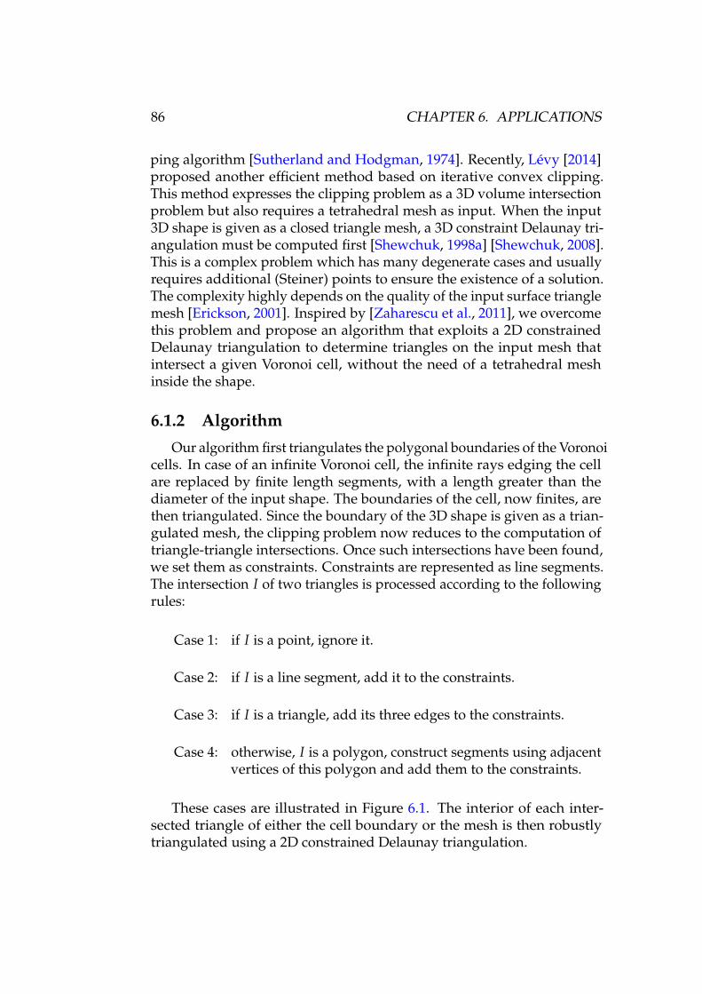
86 CHAPTER 6. APPLICATIONS

ping algorithm [Sutherland and Hodgman, 1974]. Recently, Levy [2014]proposed another efficient method based on iterative convex clipping.This method expresses the clipping problem as a 3D volume intersectionproblem but also requires a tetrahedral mesh as input. When the input3D shape is given as a closed triangle mesh, a 3D constraint Delaunay tri-angulation must be computed first [Shewchuk, 1998a] [Shewchuk, 2008].This is a complex problem which has many degenerate cases and usuallyrequires additional (Steiner) points to ensure the existence of a solution.The complexity highly depends on the quality of the input surface trianglemesh [Erickson, 2001]. Inspired by [Zaharescu et al., 2011], we overcomethis problem and propose an algorithm that exploits a 2D constrainedDelaunay triangulation to determine triangles on the input mesh thatintersect a given Voronoi cell, without the need of a tetrahedral meshinside the shape.

6.1.2 Algorithm

Our algorithm first triangulates the polygonal boundaries of the Voronoicells. In case of an infinite Voronoi cell, the infinite rays edging the cellare replaced by finite length segments, with a length greater than thediameter of the input shape. The boundaries of the cell, now finites, arethen triangulated. Since the boundary of the 3D shape is given as a trian-gulated mesh, the clipping problem now reduces to the computation oftriangle-triangle intersections. Once such intersections have been found,we set them as constraints. Constraints are represented as line segments.The intersection I of two triangles is processed according to the followingrules:

Case 1: if I is a point, ignore it.

Case 2: if I is a line segment, add it to the constraints.

Case 3: if I is a triangle, add its three edges to the constraints.

Case 4: otherwise, I is a polygon, construct segments using adjacentvertices of this polygon and add them to the constraints.

These cases are illustrated in Figure 6.1. The interior of each inter-sected triangle of either the cell boundary or the mesh is then robustlytriangulated using a 2D constrained Delaunay triangulation.

6.1. CLIPPED VORONOI TESSELLATION 87

(a) (b)

(c) (d) (e)

(f) (g) (h)

(i) (j)

Figure 6.1 – Different intersection cases. Constraints (line segments) areshown in red. (a, b) Case 1. (c, d, e) Case 2. (f, g, h) Case 3. (i, j) Case 4.(b,e,h) represent singularities.


Our clipping algorithm is summarized below (Algorithm 2). Figure6.2 depicts its main steps.

Algorithm 2: Clipping algorithm.Data: cell Ω, 3D shape V bounded by a triangulated mesh SResult: clipped cell Ω′

SΩ := TriangulateBoundary(Ω);I := Intersection(SΩ, S);if I not empty then

T := IntersectedTriangles(SΩ, I);for each triangle t of T do

T1 := ConstrainedDelaunay(t, I);for each triangle t1 of T1 do

if IsInside(t1, V) thenAdd(t1, Ω′);

endend

endT := IntersectedTriangles(S , I);for each triangle t of T do

T2 := ConstrainedDelaunay(t, I);for each triangle t2 of T2 do

if IsInside(t2, Ω) thenAdd(t2, Ω′);

endend

endendelse

Ω′ := Ω;end

6.1.3 Experimental Results

Our algorithm is implemented in C++ and we use the CGAL library[CGAL] for linear geometry Kernel which defines data structures andtheir operations. All computations were performed on an Intel XeonE5-2643 with 3.30 GHz CPU.

6.1. CLIPPED VORONOI TESSELLATION 89

(a) (b) (c)

(d) (e)

Figure 6.2 – Clipping algorithm. (a) Input: a Voronoi cell and a 3D shape(here: a closed ball) bounded by a mesh. (b) Constrained Delaunaytriangulations of the boundary of the cell and of the mesh. (c) In green:boundary of the cell inside the closed ball. (d) In blue: part of the meshinside the cell. (e) Result: the clipped cell is bounded by the green and theblue triangulations.

Computation times for our clipping method are shown in Table 6.1. Inparticular, we have tested this method on complex and badly triangulatedshapes and scenes to show its efficiency and robustness, see Figure 6.3.

6.1.4 Discussion

The advantage of our clipping algorithm is to reduce a 3D problemto 2D. It eliminates many complicated degenerate case and facilitates theprocess. The most costly part of our clipping algorithm is the computationof intersections between triangles for which we use the CGAL KernelExact predicates exact constructions kernel which is not efficient enough. Theperformance of our algorithm would be much improved if an adaptive


Figure 6.3 – More examples of clipped (non Centroidal) Voronoi diagrams.Left: input triangulations. Right: clipped Voronoi diagrams.

6.2. SHAPE ANIMATION WITH COMBINED CAPTURED ANDSIMULATED DYNAMICS 91

Shape Figure Vertices (k) Triangles (k) Sites (k) Time (s)Homer 4.8 10 20 35 28.66

Ball 4.7 0.5 1 1 0.55Bunny 4.9 10 20 50 30.06Kitten 4.9 10 20 80 54.57

Armadillo 4.9 173 346 100 103.06Ballgame 6.3 12.4 24.8 10 17.92Dancer 6.3 15.1 30.2 5 10.52Dragon 6.3 100 200 0.1 1.89Dragon 6.3 100 200 1 6.14Dragon 6.3 100 200 10 21.26Dragon 6.3 100 200 100 99.09

CAD model 6.3 182 364 100 269.67

Table 6.1 – Computation times for clipped Voronoi diagrams.

and more efficient geometry kernel could be used. Furthermore, our algo-rithm is currently implemented on CPU, a GPU version would probablybe much faster.

6.2 Shape Animation with CombinedCaptured and Simulated Dynamics

In this section, we introduce an application of shape animation usingCVTs. A novel framework is proposed to deal with the capture, shapetracking and animation generation. We consider CVTs in order to applycombined kinemamtic and physical constraint over cells using rigid bodysimulations. Moreover, regular and uniform cells ease the implementationof local constraints such as physical constraints for simulation or localdeformation constraints when tracking shapes over time sequences.

6.2.1 Introduction

Creation of animated content has become of major interest for manyapplications, notably in the entertainment industry, where the ability toproduce animated virtual characters is central to video games and specialeffects. Plausibility of the animations is a significant concern for such


productions, as they are critical to the immersion and perception of theaudience. Because of the inherent difficulty and necessary time requiredto produce such plausible animations from scratch, motion capture tech-nologies are now extensively used to obtain kinematic motion data as abasis to produce the animations, and are now standard in the industry.

However, motion capture is usually only the first stage in a com-plicated process, before the final animation can be obtained. The taskrequires large amounts of manual labor to rig the kinematic data to asurface model, correct and customize the animation, and produce thespecifics of the desired effect. This is why, in recent times, video-based3D performance capture technologies are gaining more and more atten-tion, as they can be used to directly produce 3D surface animations withmore automation, and to circumvent many intermediate stages in this pro-cess. They also make it possible to automatically acquire complex scenes,shapes and interactions between characters that may not be possible withthe standard sparse-marker capture technologies. Still, the problem ofcustomizing the surface animations produced by such technologies toyield a modified animation or a particular effect has currently no generaland widespread solution, as it is a lower level representation to beginwith.

In this work, we propose a novel system towards this goal, whichproduces animations from a stream of 3D observations acquired with avideo-based capture system. The system provides a framework to pushthe automation of animation generation to a new level, dealing with thecapture, shape tracking, and animation generation from end-to-end with aunified representation and solution. In particular, we entirely circumventthe need for kinematic rigging and present results in this report obtainedwithout any manual surface correction.

Although the framework opens many effect possibilities, for the pur-pose of the demonstration here, we focus our effort on combining thereal raw surface data captured with physics and procedural animation,in particular using a physics-based engine. To this aim, we propose touse regular Voronoi tessellations to decompose acquired shapes into vol-umetric cells, as a dense volume representation upon which physicalconstraints are easily combined with the captured motion constraints.Hence, shape motions can be perturbed with various effects in the anima-tion, through forces or procedural decisions applied on volumetric cells.Motion constraints are obtained from captured multi-view sequences oflive actions. We do not consider skeletal or surfacic motion models forthat purpose but directly track volumetric cells instead. This ensures highflexibility in both the class of shapes and the class of physical constraints


that can be accounted for. We have evaluated our method with variousactor performances and effects. We provide both quantitative results forthe shape tessellation approach and qualitative results for the generated3D content. They demonstrate that convincing and, to the best of ourknowledge, unprecedented animations can be obtained using video-basedcaptured shape models.

In summary, this work considers video-based animation and takesthe field a step further by allowing for physics-based or procedural ani-mation effects. The core innovation that permits the combination of realand simulated dynamics lies in the volumetric shape representation wepropose. The associated tessellated volumetric cells can be both trackedand physically perturbed hence enabling new computer animations.

6.2.2 Related Work

This work deals with the combination of simulated and captured shapemotion data. As mentioned earlier, this has already been explored withmarker based mocap data as kinematic constraints. Following the workof Popovic and Witkin [1999], a number of researchers have investigatedsuch combination. They propose methods where mocap data can beused either as reference motion [Popovic and Witkin, 1999] [Zordan andHodgins, 2002] [Sulejmanpasic and Popovic, 2005], or to constrain thephysics-based optimization associated to the simulation with human-likemotion styles [Safonova et al., 2004] [Liu et al., 2005] [Ye and Liu, 2008][Wei et al., 2011]. Although sharing conceptual similarities with thesemethods, our work differs substantially. Since video-based animationsalready provide natural animations, our primary objective is not to con-strain a physical model with captured kinematic constraints but rather toenhance captured animations with user-specified animation constraintsbased on physics or procedural effects. Consequently, our simulationsare not based on biomechanical models but on dynamic simulations ofmechanical effects. Nevertheless, our research draws inspiration fromthese works.

With the aim to create new animations using recorded video-basedanimations, some works consider the concatenation of elementary seg-ments of animations, e.g . [Casas et al., 2013], the local deformation ofa given animation, e.g . [Cashman and Hormann, 2012], or the transferof a deformation between captured surfaces, e.g . [Sumner and Popovic,2004]. While we also aim at generating new animations, we tackle a dif-ferent issue in this research with the perturbation of recorded animationsaccording to simulated effects.


Our method builds on results obtained in video-based animations withmulti-camera setups, to obtain the input data of our system. Classically,multi-view silhouettes can be used to build free viewpoint videos usingvisual hulls [Matusik et al., 2000] [Gross et al., 2003] or to fit a syntheticbody model [Carranza et al., 2003]. Visual quality of reconstructed shapemodels can be improved by considering photometric information [Starckand Hilton, 2007] [Tung et al., 2009] and also by using laser scanned mod-els as templates that are deformed and tracked over temporal sequences[De Aguiar et al., 2007] [Vlasic et al., 2008] [De Aguiar et al., 2008]. Inter-estingly, these shape tracking strategies provide temporally coherent 3Dmodels that carry therefore motion information. In addition to geometricand photometric information, considering shading cues allows to recoverfiner scale surface details as in [Vlasic et al., 2009] [Wu et al., 2012].

More recent approaches have proposed to recover both shapes andmotions. They follow various directions depending on the prior informa-tion assumed for shapes and their deformations. For instance in the caseof human motion, a body of work assumes articulated motions that can berepresented by the poses of skeleton based models, e.g . [Vlasic et al., 2008][Gall et al., 2009] [Straka et al., 2012]. We base our system on a differentclass of techniques aiming at more general scenarios, with less constrainedmotion models simply based on locally rigid assumptions in the shapevolume [Allain et al., 2015]. This has the advantage that a larger classof shapes and deformations can be considered, in particular motions ofhumans with loose clothes or props. The technique also has the significantadvantage that it allows to track dense volumetric cell decompositions ofshapes, thereby allowing for consistent captured motion information tobe associated and propagated with each cell in the volume, a key propertyto build our animation generation framework on.

In the following, we provide a system overview, followed by a detailedexplanation of how we tessellate 3D input observations into regular poly-hedral cells, to be subsequently tracked and used as primary animationentity (see Section 6.2.4). In order to recover kinematic constraints fromreal actions, our system then tracks polyhedral cells using surface obser-vations and a locally rigid deformation model (see Section 6.2.5). Finally,a physics or procedural simulation integrates the animation constraintsover the shape (see Section 6.2.6). To our knowledge, this is the first at-tempt to propose such an end-to-end system and framework to generateanimations from real captured dynamic shapes.


6.2.3 System Overview

(a) (b)

(c) (d)

Figure 6.4 – From video-based shape capture to physic simulation. (a)Original videos. (b) Volumetric shape representations. (c) Volumetricshape tracking (template in blue). (d) Physics-based simulation. Theapproach uses multiple videos and Voronoi tessellations to capture thevolumetric kinematic of a shape motion which can then be reanimatedwith additional mechanical effects, for instance volumetric erosion withgravity in the figure.

We generate a physically plausible animation given a sequence of 3Dshape observations as well as user specifications for the desired effectto be applied on the animation. 3D observations are transformed intotemporally consistent volumetric models using centroidal Voronoi tessel-lations and shape tracking. Kinematic and physical constraints are then


combined using rigid body physics simulation. The approach involvesthe following main steps depicted in Figure 6.4.

6.2.3.1 Video Based Acquisition

Input to our system are 3D observations of a dynamic scene. Tra-ditional and probably most common dynamic scenes in graphics arecomposed of human movements; however our system can consider alarger class of shapes since only local rigidity is assumed to get temporallyconsistent shape models. 3D observations are assumed to be obtainedusing a multi-camera system and can be in any explicit, e.g . meshes orimplicit, e.g . from point clouds through Poisson function, forms. Ourown apparatus is composed of 68 calibrated and synchronized cameraswith a resolution up to 2048× 2048 pixels. The acquisition space is about8m× 4m and the camera frame rate can go up to 50 fps at full resolution.The outputs of this step are point clouds with around 100k points.

6.2.3.2 Volumetric Representation

Input 3D observations are tessellated into polyhedral cells. This volu-metric representation is motivated by two aspects of our animation goal:first, the representation is well suited to physical simulation; second, volu-metric deformation models are more flexible than skeleton based models,hence enabling non rigid shape deformations. Still, they allow for locallyrigid volumetric constraints, a missing feature with surface deformationmodels when representing shapes that are volumes. We adopt centroidalVoronoi tessellations since they produce regular and uniform polyhedralcells.

6.2.3.3 Tracking

In this step, incoherent volumetric shape models of a temporal se-quence are transformed into coherent representations where a singleshape model is evolving over time. This provides kinematic informationat the cell level that will further be used in the simulation. We use a track-ing method [Allain et al., 2015] that finds the poses of a given templateshape at each frame. The template shape is taken as one of the volumetricmodels at a frame. The approach uses a volumetric deformation model,instead of surface or skeleton based model, to track shapes. It optimizesthe pose of the template shape cells so as to minimize a distance cost toan input shape model while enforcing rigidity constraints on the local cellconfigurations.


6.2.3.4 Simulation

The tracked cell representation is both suitable for tracking and conve-nient for solid based physics. We embed the tracked volumetric model ina physical simulation, by considering each cell to be a rigid solid shapein mechanical interaction with other cells and scene shapes. We ensurecohesion of cells by attaching a kinematic recall force in the simulation,and offer various controls as to how the scene may deform, collide, orrupture during contacts and collisions. This simple framework allows fora number of interesting effects demonstrated in 6.2.7.

6.2.4 Volumetric Shape Modeling

As mentioned before, we compute CVTs of input observations becausecombined kinematic and physical constraints can be easily applied overcells using rigid body simulations. Moreover, CVTs provide regular anduniform cells that ease the implementation of local constraints or deforma-tion constraints compared with voxel- and Delaunay-based tessellations.Figure 6.5 shows the comparison of the three approaches. For more detailsabout the construction of CVTs from implicit shapes and the comparisonof the three approaches, please see Chapter 5.

6.2.5 Volumetric Shape Tracking

With the volumetric decomposition proposed above, we now needto define a model by which scene dynamics can be captured throughdeformations expressed over this decomposition. We consider here asinput a time sequence of inconsistent CVT decompositions independentlyestimated at each frame and we look for a time consistent volumetricdecomposition that encode cell motions. We opt for a capture by deforma-tion approach where a template CVT, taken from the input sequence inour case, is tracked throughout the sequence. This volumetric strategy ismotivated by two observations. First, attaching the deformation model tothe cell shape representation used for the animation directly provides thenecessary cell dynamic information to the simulation. It avoids thereforethe interpolation between an intermediate motion model, e.g . a skeletonor a mesh, and the animation model; Such interpolation being difficult toperform consistently over time. Second, as shown in [Allain et al., 2015],it provides a simple tool for embedding volume-preservation constraintsthat increase the robustness of the tracking over the dynamic scenes we


(a) (b)

(c) (d)

(e) (f)

(g) (h)

Figure 6.5 – (a, b) Input multi-camera observation and point clouds (65386pts). (c, d) Tessellations generated using voxels [Chernyaev, 1995]. (e, f)Tetrahedrisations generated using Delaunay refinement [CGAL]. (g, h)Clipped Centroidal Voronoi Tessellations (14455 sites).


consider. We describe below the generative approach [Allain et al., 2015]that we follow.

6.2.5.1 Tracking Formulation

We are given a sequence of CVTs V and a template model V. V canbe one model taken from the sequence or any other model (e.g . a 3Dscan) decomposed into a CVT. The tracking consists then in fitting V toeach V ∈ V . This can be formulated as a maximum a posteriori (MAP)estimation of the deformation parameters Θ that maximizes the posteriordistribution P(Θ|V) of the parameters Θ given the observations V :

Θ = arg maxΘ

P(Θ|V) ' arg maxΘ

P(V|Θ) P(Θ).

Taking the log of the above expression yields the following optimiza-tion problem:

Θ = arg maxΘ

Edata(V , Θ) + Eprior(Θ), (6.1)

where the data term Edata evaluates the log-likelihood of a set of deforma-tion parameters Θ given the observations V , and the regularization termEprior enforces prior constraints on the deformation, e.g . local rigidity. Wedetail below the parameterization Θ we use for the deformation and theassociated energy terms.

6.2.5.2 Motion Parameterization

The deformation model is defined over CVT cells in the shape de-composition and, for efficiency, on aggregates of cells which reduces thenumber of terms and parameters. To this goal, CVT cells are groupedtogether as a set of volumetric patches Pk using a k-medoids algorithm, asshown in Figure 6.6. Such patches can be either adjacent to the surface orcompletely inside the template shape’s volume, which is of particular in-terest to express non-rigid deformation of the model while preserving thelocal volume and averting over-compression or dilation. The positionalinformation of a patch is represented as a rigid transform Tt

k ∈ SE(3)at every time t. Each position xk,q of a CVT sample is indiscriminatelylabeled as a point q. Its position can be written as a transformed versionof its template position x0

q as follows, once the patch’s rigid transform isapplied:


Figure 6.6 – The template model used to recover the runner sequencemotion, with its CVT decomposition cells, and the cell clusters in differentcolors.

xk,q = Tk(x0q). (6.2)

A pose of the shape is thus defined as the set of patch transformsT = Tkk∈K, which expresses the deformation of every component inthe shape. The parameterization Θ is then the set of pose parameters ofthe template over the considered time sequence T :

Θ = Ttt∈T .

6.2.5.3 Data Term

We assume the observed shape Vt at time t is described by the pointcloud Yt = yt

o. We assume this point cloud to include inner volumepoints and surface points, i.e . the CVT sites as well as the outside surfacepoints.

In order to measure how a deformed version of the template explainsthe observed shape, first the associations between the observations andthe template must be determined. This is achieved via a soft ICP strategythat iteratively reassigns each observation yt

o to the template volumetricpatches. For simplicity, each observation yt

o is associated to the patch


Pk via the best candidate point xk,q of patch Pk and with an associationpenalty αo,k.

The matching penalty E(yto, Tt

k) that evaluates how well Pk explainsyt

o is then the weighted distance between yto and the best candidate xk,q,

that is the template point x0q transformed by the current pose Tt

k of thetemplate model:

E(yto, Tt

k) = αto,k‖y

to − Tt

k(x0q)‖. (6.3)

Associations are additionally filtered using a compatibility test. Ob-served surface points are associated to template surface points with similarorientations with respect to a user defined threshold θmax; Observed in-ner points are associated to template inner points that present similardistances to the surface up to a user defined tolerance ε. If there is nocompatible candidate in a patch Pk, then Pk is discarded for the associationwith yt

o, i.e . αto,k = 0. Finally:

Edata(Vt, Θt) = ∑o,k

E(yto, Tt

k). (6.4)

6.2.5.4 Regularization Term

The pose of a shape is defined by the set of rigid motion parameters ofthe shape volumetric patches. While these parameters hardly constraintthe patch motions, they do not define a coherent shape motion since eachpatch moves independently of the others. In order to enforce shape cohe-sion, soft local rigidity constraints, reflecting additional prior knowledgeon shape deformation parameters, are considered. These constraints relyon a pose distance function that evaluates how distant from a rigid trans-formation a deformation between two poses is. Once such a distance isdefined, the regularization term is defined as the sum of distances be-tween all poses in the sequence and a given pose that can be a referencepose or an estimated mean pose, as explained below.

Pose Distance

To simplify the estimation, the shape distance is expressed over coor-dinates of points belonging to patches and not on the parameters of thepose itself:


D(Ti, Tj) = ∑(Pk ,Pt)∈N

Dkl(Ti, Tj), with (6.5)

Dkl(Ti, Tj) = ∑q∈Pk∪Pl

‖Tik−l(x

0q)− Tj

k−l(x0q)‖2, (6.6)

where Tik−l = Ti−1

l Tik is the relative transformation between patches

Pk and Pl for pose i, and N is the set of neighboring patch pairs withinthe shape. Intuitively, this distance measures whether the relatives posesbetween neighboring volumetric patches are preserved during motionbetween two shape poses.

Deformation Energy

The pose distance above allows to compute a deformation energybetween two poses and with respect to a reference pose from whichthe patch transformations Tk

t are expressed. This reference pose can betaken as the identity pose of the initial template model (see Figure 6.6 forinstance). However such a strategy is biased toward the template poseand discourage locally rigid motions between poses that are distant fromthe template pose. A more appropriate approach is to exploit the posedistance function to first define a mean pose T over a time window t:

T = arg minT

∑tD(Tt, T).

This averaged pose can then be taken as an evolving reference posefrom which non-rigid deformations are measured to define the deforma-tion energy over the associated time interval:

E(Tt, T) = ∑tD(Tt, T). (6.7)

This imposes general proximity of poses to a sequence specific ”rest”pose. These rest poses must also be constrained to some form of innercohesion. This is ensured by minimizing the distance from the mean poseto the identity pose of our initial template:

E(T) = D(T, Id). (6.8)

This definition of deformation has a number of advantages: first itenforces geometric cohesion and feature preservation, and second it isquite simple to formulate and to optimize, as the minimization of (6.7)


and (6.8) translates to a sum of least square constraints over the set of CVTsites.The prior energy term finally writes:

Eprior(Θ = Tt) = D(T, Id) + E(T, T). (6.9)

We jointly extract poses and a sequence mean pose by minimizing thesum of the data terms (6.4) and the prior term (6.9). Section 6.2.7 showsresults on various sequences and gives run time performances.

6.2.6 Combined Animation

The template representation of the subject now being consistentlytracked across the sequence, we can use the tracked cells as input forsolid physics-based animation. We have purposely chosen CVTs as acommon representation as they can be made suitable for shape and motioncapture as we have shown, while being straightforwardly convenient forphysics-based computations. In fact CVT cells are compact, convex oreasily approximated by their convex hull. This is an advantage for thenecessary collision detection phase of physics models, as specific andefficient algorithms exist for this case [Gilbert et al., 1988] [Rabbitz, 1994].We here describe the common principles of our animation model, withmore specific applications being explored and reported on in the followingsections.

As our animation framework is solid-based, we base our descriptionon commonly available solid-based physics models, e.g . [Baraff, 1997].Each CVT cell is considered a homogeneous rigid body, whose simulatedstate is parameterized by its 3D position, rotation, linear momentum andangular momentum. The cell motion is determined by Newton’s lawsthrough a differential equation involving the cell state, the sum of forcesand sum of torques that are applied to the cell.

The animation is thus obtained by defining the set of forces and torquesapplied at each instant, and iteratively solving these differential equationsto obtain a new cell position and orientation for a target time step, usingone of many available techniques. For our demonstrator, we use thesimple and efficient off-the-shelf Bullet Physics engine [Coumans et al.,2013] [Catto, 2005].

6.2.6.1 Ordinary Applied Forces

We classically apply the constant gravity force Fg = Mg. We applyadditional external forces or constraints as needed for the target appli-cation, as will be detailed in the coming sections. Additionally, contact


forces such as collisions are handled with scene shapes, as well as betweendifferent cells of the CVT. For this purpose the physics engine first needsto detect the existence of such contacts. It relies on a hierarchical spacedecomposition structure, such as an AABB-tree, for broad-phase collisiondetection, i.e . coarse elimination of collision possibilities. A narrow-phasecollision test follows, between shapes lying in the same region of spaceas determined by the AABB-tree traversal. In this narrow phase the fullgeometry of shapes is examined, e.g . using the GJK algorithm [Gilbertet al., 1988] for pairs of convex polyhedra. Once the existence of a contactis established, various strategies exist to deal with the collision, e.g . byintroducing impulse repulsion forces to produce a collision rebound. Wefollow the common approach of modeling contacts as a linear complemen-tary problem (LCP) popularized by [Baraff, 1994], which derives contactforces as the solution of a linear system that satisfies certain inequalityconstraints. These constraints are typically formulated using a constraintJacobian over the combined state spaces of rigid bodies. [Catto, 2005]expose the specific variant applied in the context of the Bullet Physicsengine.

6.2.6.2 Physical Modeling of Kinematic Control

To relate the physical simulation to the acquired non-rigid poses of themodel, we need to introduce coupling constraints. Our goal is to allowthe model to materialize and control the tradeoff between the purely kine-matic behavior acquired from visual inputs for the cell, and the purelymechanically induced behavior in the simulation. First it is important tonote that the temporal discretization used for acquisition and for simu-lation and rendering of the effects are generally different. Consequentlythe first stage in achieving our goal is to compute a re-sampling of thepose sequence, to the target simulation and rendering frequency, usingposition and quaternion interpolation. The poses so obtained are herereferred as the acquired cell poses xa(t) and Ra(t). Second, we formulatethe coupling by introducing a new kinematic recall force, in the form ofa damped spring between the acquired cell poses and the simulated cellposes:

Fr(t) = k.(xa(t)− x(t))− λ.ddt

(xa(t)− x(t)), (6.10)

where k and λ are respectively the rigidity and damping coefficients of thespring, which control the strength and numerical stability of the coupling.


6.2.7 Visual Effects

Figure 6.7 – An animation that combines video-based shape motion (left)and physical simulation (right). Our method allows to apply mechanicaleffects on captured dynamic shapes and generates therefore plausibleanimations with real dynamics.

This section presents various animation results on three captured ani-mations of variable nature and speed. RUNNER shows a male characterrunning in a straight line, during 3 motion cycles. This animation lasts2.5 s. In CAGEBIRDDANCE a female dancer moves while holding a birdcage. This sequence is 56 s long and shows a complex sequence of mo-tions which would be difficult to synthesize without sensors. Finally, inSLACKLINE a male acrobat evolves on a non rigid line above the ground,for 25 s. The input sequences of temporally inconsistent 3D point cloudsare made respectively of 126 (RUNNER), 2800 (CAGEBIRDDANCE) and1240 (SLACKLINE) temporal frames.

Parameters

The interior of all shapes has been tessellated according to 6.2.4 using5000 cells. 10 iterations of the L-BFGS quasi-Newton algorithm wereapplied, except for the template shape where 50 iterations were applied.We use a temporal window of 10 frames for the tracking, and cluster the5000 cells into 200 patches. 60 iterations were applied.

We list below examples of visual effects that we were able to generateusing the proposed approach. First, we present animations combiningtracking results with solid dynamics simulation (6.2.7.1). Then we presentother visual effects that also exploit the volumetric tracking information(6.2.7.2 and 6.2.7.3).


6.2.7.1 Asynchronous Kinematic Control Deactivation

In order to show the effect of gravity while keeping the dynamicmotion of the input sequence, we deactivate kinematic control forcesindependently for each cell. After being deactivated, a cell usually fallsto the ground, since it follows a trajectory determined only by gravity,collision forces and its initial velocity. Asynchronous cell deactivationsresult in an animation combining cells that follow their tracking trajectoryand cells that fall. By choosing diverse strategies for scheduling celldeactivations, a wide variety of animations can be obtained.

We explore here three possible deactivation strategies that are basedon different criteria. Note that while these effects are straight-forward toproduce with our volumetric framework, it would be difficult to obtainthem if only surface or skeleton-based tracking was available.

6.2.7.1.1 Rupture under Collisions

Collisions with obstacles sometimes deviate a cell from its theoreticaltrajectory, which results in an increase of the recall force magnitude (seeEq. 6.10). This phenomenon can be detected and used for simulating therupture of the material: when the recall force magnitude of a cell is abovea given threshold, we deactivate the recall force (for this cell only). Thismakes the rupture looks like the consequence of the collision.

Figure 6.8 shows a heavy pendulum that hits the subject and makesa hole in it. Under the intensity of the collision, several cells are ejected(rupture) and fall to the ground.

6.2.7.1.2 Heat Diffusion

In order to make the cell deactivation both temporally and spatiallyprogressive, we rely on a diffusion algorithm. We diffuse an initial temper-ature distribution inside the volume according to the diffusion equation.Deactivation is triggered when the cell temperature is above a giventhreshold.

Heat diffusion in a CVT

The CVT provides a graph structure on centroids, which is a sub-graph of the Delaunay tetrahedralization of the cells centroids. The heatdiffusion on a graph structure is expressed by the heat equation:

(∂/∂t + L)Ft = 0,


Figure 6.8 – Input SLACKLINE Multi-camera observations (left), trackingresult of the SLACKLINE sequence (top) and combination with the effectof collision with a pendulum (bottom).


where Ft is the column vector of centroids temperatures at time t, and L isthe combinatorial graph Laplacian matrix (note that a geometric Laplacianis not necessary since centroids are regularly distributed in space). Givenan initial temperature distribution F0, this equation has a unique solution

Ft = HtF0,

where Ht = etL is the heat diffusion kernel, which can be computed bymeans of the spectral decomposition of L.

We compute the temperature evolution on the CAGEBIRDDANCE se-quence for an initial temperature distribution where all cell temperaturesare zero, except for the dancer’s head top cells (which are set to 1). Weobserve in Figure 6.7 that cells fall progressively across time, from theupper to the lower body parts. Note that the cage cells remain kinemati-cally controlled since heat is not transferred between different connectedcomponents.

6.2.7.1.3 Morphological Erosion

The discrete cell decomposition of shapes allows to apply morphologi-cal operators. To illustrate this principle, we have experimented erosionas shown in Figure 6.4. In this example, cells are progressively erodedstarting from the outside. The morphological erosion is performed bydeactivating each cell after a delay proportional to the distance betweenthe cell centroid and the subject’s surface. The distance is computed onlyonce for each cell, on the template shape. Figure 6.4 shows the erosion an-imation on the RUNNER sequence. Note that the operation progressivelyreveals the dynamic of the inner part of the shape.

6.2.7.2 Time Persistence

In this example, we experiment time effects over cell decompositions.To this aim, dynamic copies of the model are generated at regular timeintervals. These copies are equipped with deceleration and erosion effectsover time and create therefore ghost avatars that vanish with time (seeFigure 6.9). The benefit of the tracked volumetric representation in thissimulation is the ability to attach time effect to the model behavior at thecell level, for instance lifetime and deceleration in the example.


Figure 6.9 – Time persistence on the RUNNER sequence: a slower copy ofthe shape that erodes over time is generated at regular intervals.

6.2.7.3 Morphing

Our dynamic representations allows to apply volumetric morphingbetween evolving shapes, enabling therefore new visual effects with realdynamic scenes. To this purpose, cells of the source shape are first matchedto the target shape. Second, each cell is individually morphed to its targetcell at a given time within the sequence. Time ordering is chosen suchthat cells in the source shape are ordered from the outside to the inside,and associated with the cells of the target shape ordered from the insideto the outside. Cells are transformed from the source to the destinationby interpolating their positions and using Kent et al. [1992] to morphtheir polyhedral shapes. Figure 6.10 shows the dynamic morphing of theRUNNER sequence onto the CAGEBIRDDANCE sequence.

6.2.7.4 Run Time Performance

Our approach has been tested on a dual Intel Xeon E5-2665 processorwith 2.40 GHz each. For each animation, the Poisson runs in 0.67 s perframe on average, and the volumetric decomposition for each frame runsin 6.27 s, except for the template model for which it runs in 25.52 s since


Figure 6.10 – Tracking result of the RUNNER and the CAGEBIRDDANCEsequences (middle) and combination with volumetric morphing with5000 cells (bottom).


more iterations are applied. Our tracking algorithm runs in 45 s perframe on average. The physical simulation usually needs about 350 msper simulation step on a single thread. The morphing runs on multiplethreads in about 2.35 s.

6.2.8 Limitations

As shown in the previous examples, our approach generates plausibleresults for a variety of captured and simulated motions. However, afew limitations must be noted. First, the true captured shape must bevolumetric in nature, since we tessellate its interior into 3D cells. Thinshapes such as clothes may cause some cells to be flat, leading to volumevariation among cells and ill-defined cohesion constraints that wouldcause difficulty to the tracking model.

Regarding the physical simulation, our current demonstrator is lim-ited to rigid body interactions, but could be extended to other physicalmodels such as soft body physics and fluid simulation. Since a CVT pro-vides neighboring information, soft body simulation could be achievedby introducing soft constraints between neighboring cells. This wouldlead to animations where cell sets behave more like a whole rather thanindependent bodies.

6.2.9 Conclusion

We have proposed a framework that allows video-based animations tobe combined with physical simulation to create unprecedented and plau-sible animations. Our approach benefits of both regularity and uniformityof CVTs. Both volumetric shape tracking and animation generation in ourframework rely on CVTs to perform well.

Chapter 7

Conclusion

Contents7.1 Summary of Contributions . . . . . . . . . . . . . . . . 1137.2 Future Research Perspectives . . . . . . . . . . . . . . . 114

In this thesis, we have focused on the problem of regular volumetrictessellation based on centroidal Voronoi tessellations. Our contributionsare threefold: (1) propose criteria to evaluate quantitatively the regularityof volumetric tessellations; (2) introduce a novel algorithm that build CVTswith better regularity than the state-of-the-art methods; (3) extend CVT toimplicit shapes and build an extensive comparison of voxel-, Delaunay-and Voronoi-based approaches for approximated volumetric tessellations.

This chapter is organized as follows: In Section 7.1, we summarize thecontributions of this thesis. Future work perspectives inspired from thework done in this thesis are provided in Section 7.2.

7.1 Summary of Contributions

In Chapter 3, we have built a theoretical work on the regularity ofvolumetric tessellations. Based on the normalized second order moments,we have proposed criteria that allow to evaluate and compare the regu-larity of tessellations. We have also shown that these criteria are linkedto the CVT energy function which allows to compute the value of theoptimal CVT energy given a shape and a number of sites. We have alsoproposed a novel stopping criterion defined by this optimal value for theCVT algorithm as an application.

In Chapter 4, we have proposed a hierarchical algorithm for regularCVTs. The experimental results have shown that the subdivision schema

113

114 CHAPTER 7. CONCLUSION

of our algorithm preserves the local optimality of CVTs on unboundeddomains. With a relatively large number of inner cells than boundarycells, our algorithm builds more regular CVTs with better efficiency thanthe state-of-the-art algorithms.

In Chapter 5, we have extended the CVT algorithm to implicit shapes.In order to have a good approximation to the implicit shape, a local im-provement has been proposed to clip the CVT. We have also presentedan extensive comparison of the existing methods and ours in terms ofaccuracy, regularity and computational time. The experimental resultshave shown that our algorithm performs the best except for the computa-tional time. This is because our algorithm includes an unavoidable step ofDelaunay triangulation that is relatively costly compared to the MarchingCubes algorithm.

In Chapter 6, a novel algorithm has been proposed to clip Voronoitessellations. The variant experimental results have shown its robustness.We have also proposed another application that is a shape animationframework using CVTs. This framework benefits from the propertiesof CVTs so that it allows to combine kinematic and physical constraintsusing rigid body simulation.

7.2 Future Research Perspectives

In the following, we gives some perspectives for further research basedon the contributions in this thesis.

Theoretical Work on CVT

CVTs correspond to local minima of the energy function and an opti-mal CVT achieves the global minimum of this function. However, sincethe CVT energy function is non linear and non convex, it appears to bevery difficult to find its global minimum. Lu et al. [2012] have proposed astochastic approach that tries to find all local minima of the CVT energyfunction in order to find the global minimum. This approach can theoreti-cally achieve the global minimum in infinite computational time whichleads to inefficient computation in practice. According to our study on therelation between our regularity criteria and the energy function, we cancompute the global minimum of this function for any three-dimensionalshape. This allows to measure how close a CVT is to its optimal one.However, our work is based on Gersho’s conjecture [Gersho, 1979] thathas not been proven in three dimensions. We also assume that the effect of

7.2. FUTURE RESEARCH PERSPECTIVES 115

shape boundary is negligible. It would be worth exploring this theoreticalwork. In practice, it would be also interesting to eliminate the effect ofshape boundary or to determine the number of sites necessary to neglectthis effect for a given shape.

Generalized CVT Algorithm

In this thesis, we have proposed a CVT algorithm for implicit shapes.Since this is the first algorithm to build CVTs of implicit shapes, manyextensions such as weighted Voronoi tessellations and power diagramscan be investigated. Levy and Liu [2010] have introduced a generalizedCVT whose energy function uses a Lp distance instead of the Euclideandistance. This generalized distance allows to change the shape of CVTcells. It would be interesting to implement a version of this Lp CVT forimplicit shapes.

Another direction is to improve the performance of our CVT algorithm.For instance, in this thesis, we have also proposed a hierarchical approachin order to build regular CVTs, this approach could be easily integratedinto our CVT algorithm to improve the regularity of the generated CVTs.The experimental results have shown that our algorithm is less efficientthan the Marching Cubes algorithm. As mentioned before, this is becauseof the unavoidable Delaunay triangulation in our algorithm. One wayto reduce the computational time is to reduce the number of sites. Webelieve that applying our algorithm on a shape with non uniform densitymay achieve this purpose without losing the accuracy of generated CVTs.For instance, if we define the density near the boundary is much higherthan the one far from the boundary, our algorithm would build CVTs withlarge inner cells and small boundary cells. Thus, we reduce the numberof sites while keeping the accuracy of approximation to the shape.

Bibliography

D. Akio and A. Koide. An efficient method of triangulating equi-valuedsurfaces by using tetrahedral cells. IEICE TRANSACTIONS on Infor-mation and Systems, 74(1):214–224, 1991. Cited on page 12.

B. Allain, J.-S. Franco, and E. Boyer. An efficient volumetric frameworkfor shape tracking. In Proceedings of the IEEE Conference on ComputerVision and Pattern Recognition, pages 268–276, 2015. Cited on pages 35,36, 94, 96, 97, and 99.

B. Allain, L. Wang, J.-S. Franco, F. Hetroy, and E. Boyer. Shape anima-tion with combined captured and simulated dynamics. arXiv preprintarXiv:1601.01232, 2016. Cited on pages 1, 4, and 35.

P. Alliez, D. Cohen-Steiner, M. Yvinec, and M. Desbrun. Variational tetra-hedral meshing. In ACM Transactions on Graphics (TOG), volume 24,pages 617–625. ACM, 2005. Cited on page 25.

B. Anderson. http://www.cs.carleton.edu/cs comps/0405/shape/marching cubes.html. Cited on pages vi and 11.

F. Aurenhammer. Power diagrams: properties, algorithms and appli-cations. SIAM Journal on Computing, 16(1):78–96, 1987. Cited onpage 29.

F. Aurenhammer. Voronoi diagramsa survey of a fundamental geometricdata structure. ACM Computing Surveys (CSUR), 23(3):345–405, 1991.Cited on pages 27 and 39.

D. Baraff. Fast contact force computation for nonpenetrating rigid bodies.In Proceedings of the 21st annual conference on Computer graphicsand interactive techniques, pages 23–34. ACM, 1994. Cited on page 104.

D. Baraff. An introduction to physically based modeling: rigid bodysimulation iunconstrained rigid body dynamics. SIGGRAPH CourseNotes, 1997. Cited on page 103.

117

118 BIBLIOGRAPHY

E. Barnes and N. Sloane. The optimal lattice quantizer in three dimensions.SIAM Journal on Algebraic Discrete Methods, 4(1):30–41, 1983. Citedon page 40.

N. Barnes, G. Loy, and D. Shaw. The regular polygon detector. PatternRecognition, 43(3):592–602, 2010. Cited on page 37.

M. Berger, J. A. Levine, L. G. Nonato, G. Taubin, and C. T. Silva. Abenchmark for surface reconstruction. ACM Transactions on Graphics(TOG), 32(2):20, 2013. Cited on pages ix, 70, 76, 77, and 84.

M. Berger, A. Tagliasacchi, L. Seversky, P. Alliez, J. Levine, A. Sharf, andC. Silva. State of the art in surface reconstruction from point clouds. InEUROGRAPHICS star reports, volume 1, pages 161–185, 2014. Citedon page 8.

V. Blatov, L. Carlucci, G. Ciani, and D. Proserpio. Interpenetrating metal–organic and inorganic 3d networks: a computer-aided systematic inves-tigation. part i. analysis of the cambridge structural database. CrystEng-Comm, 6(65):378–395, 2004. Cited on pages vii and 41.

J.-D. Boissonnat and S. Oudot. Provably good sampling and meshing ofsurfaces. Graphical Models, 67(5):405–451, 2005. Cited on page 76.

A. Bowyer. Computing dirichlet tessellations. The Computer Journal, 24(2):162–166, 1981. Cited on page 18.

K. Q. Brown. Voronoi diagrams from convex hulls. Information ProcessingLetters, 9(5):223–228, 1979. Cited on page 17.

J. Bucklew. Upper bounds to the asymptotic performance of block quan-tizers. Information Theory, IEEE Transactions on, 27(5):577–581, 1981.Cited on page 39.

J. A. Bucklew and G. L. Wise. Multidimensional asymptotic quantiza-tion theory with¡ img src=”/images/tex/130. gif” alt=” r”¿ th powerdistortion measures. Information Theory, IEEE Transactions on, 28(2):239–247, 1982. Cited on page 39.

H. Carr, T. Theußl, and T. Moller. Isosurfaces on optimal regular samples.In ACM International Conference Proceeding Series, volume 40, pages39–48. Citeseer, 2003. Cited on page 12.

BIBLIOGRAPHY 119

J. Carranza, C. Theobalt, M. A. Magnor, and H.-P. Seidel. Free-viewpointvideo of human actors. ACM transactions on graphics (TOG), 22(3):569–577, 2003. Cited on page 94.

D. Casas, M. Tejera, J.-Y. Guillemaut, and A. Hilton. Interactive animationof 4d performance capture. Visualization and Computer Graphics, IEEETransactions on, 19(5):762–773, 2013. Cited on page 93.

T. J. Cashman and K. Hormann. A continuous, editable representationfor deforming mesh sequences with separate signals for time, pose andshape. In Computer Graphics Forum, volume 31, pages 735–744. WileyOnline Library, 2012. Cited on page 93.

E. Catto. Iterative dynamics with temporal coherence. In Game developerconference, volume 2, page 5, 2005. Cited on pages 103 and 104.

CGAL. Computational Geometry Algorithms Library.http://www.cgal.org/. Cited on pages vi, ix, x, 23, 63, 75, 76,84, 88, and 98.

R. Chalmeta, F. Hurtado, V. Sacristan, and M. Saumell. Measuring regu-larity of convex polygons. Computer-Aided Design, 45(2):93–104, 2013.Cited on page 37.

L. Chen and J.-c. Xu. Optimal delaunay triangulations. Journal of Com-putational Mathematics, pages 299–308, 2004. Cited on page 25.

X. Chen, A. Golovinskiy, and T. Funkhouser. A benchmark for 3d meshsegmentation. In ACM Transactions on Graphics (TOG), volume 28,page 73. ACM, 2009. Cited on pages ix, 76, 79, and 84.

S.-W. Cheng, T. K. Dey, H. Edelsbrunner, M. A. Facello, and S.-H. Teng.Silver exudation. Journal of the ACM (JACM), 47(5):883–904, 2000.Cited on pages 25 and 70.

S.-W. Cheng, T. K. Dey, and E. A. Ramos. Delaunay refinement for piece-wise smooth complexes. Discrete & Computational Geometry, 43(1):121–166, 2010. Cited on pages 23 and 74.

E. V. Chernyaev. Marching cubes 33: Construction of topologically correctisosurfaces. Institute for High Energy Physics, Moscow, Russia, ReportCN/95-17, 42, 1995. Cited on pages x, 14, 15, and 98.

L. P. Chew. Constrained delaunay triangulations. Algorithmica, 4(1-4):97–108, 1989. Cited on page 20.

120 BIBLIOGRAPHY

L. P. Chew. Guaranteed-quality mesh generation for curved surfaces. InProceedings of the ninth annual symposium on Computational geome-try, pages 274–280. ACM, 1993. Cited on page 24.

P. Chew. There is a planar graph almost as good as the complete graph.In Proceedings of the second annual symposium on Computationalgeometry, pages 169–177. ACM, 1986. Cited on page 17.

P. Cignoni, C. Montani, and R. Scopigno. Dewall: A fast divide andconquer delaunay triangulation algorithm in e d. Computer-AidedDesign, 30(5):333–341, 1998a. Cited on page 18.

P. Cignoni, C. Rocchini, and R. Scopigno. Metro: measuring error onsimplified surfaces. In Computer Graphics Forum, volume 17, pages167–174. Wiley Online Library, 1998b. Cited on pages 70 and 77.

J. H. Conway and N. Sloane. Voronoi regions of lattices, second momentsof polytopes, and quantization. Information Theory, IEEE Transactionson, 28(2):211–226, 1982. Cited on pages xi, 3, 38, 39, and 40.

E. Coumans et al. Bullet physics library. Open source: bulletphysics. org,2013. Cited on page 103.

H. Coxeter. Regular skew polyhedra in three and four dimension, andtheir topological analogues. Proceedings of the London MathematicalSociety, 2(1):33–62, 1938. Cited on page 37.

H. S. M. Coxeter. Twelve geometric essays. Southern Illinois Univ Pr, 1968.Cited on page 37.

M. Cubes. A high resolution 3d surface construction algorithm/william e.Lorensen, Harvey E. Cline–SIG 87, 1987. Cited on page 76.

L. Custodio, T. Etiene, S. Pesco, and C. Silva. Practical considerations onmarching cubes 33 topological correctness. Computers & Graphics, 37(7):840–850, 2013. Cited on page 15.

E. De Aguiar, C. Theobalt, C. Stoll, and H.-P. Seidel. Marker-less de-formable mesh tracking for human shape and motion capture. In Com-puter Vision and Pattern Recognition, 2007. CVPR’07. IEEE Conferenceon, pages 1–8. IEEE, 2007. Cited on page 94.

E. De Aguiar, C. Stoll, C. Theobalt, N. Ahmed, H.-P. Seidel, and S. Thrun.Performance capture from sparse multi-view video. ACM Transactionson Graphics (TOG), 27(3):98, 2008. Cited on page 94.

BIBLIOGRAPHY 121

B. de Araujo, D. S. Lopes, P. Jepp, J. A. Jorge, and B. Wyvill. A survey onimplicit surface polygonization. ACM Computing Surveys (CSUR), 47(4):60, 2015. Cited on page 70.

B. Delaunay. Sur la sphere vide. Izv. Akad. Nauk SSSR, Otdelenie Matem-aticheskii i Estestvennyka Nauk, 7(793-800):1–2, 1934. Cited on page 15.

Q. Du and M. Emelianenko. Acceleration schemes for computing cen-troidal voronoi tessellations. Numerical linear algebra with applications,13(2-3):173, 2006. Cited on page 33.

Q. Du and D. Wang. Tetrahedral mesh generation and optimization basedon centroidal voronoi tessellations. International journal for numericalmethods in engineering, 56(9):1355–1373, 2003. Cited on page 25.

Q. Du, V. Faber, and M. Gunzburger. Centroidal voronoi tessellations:applications and algorithms. SIAM review, 41(4):637–676, 1999. Citedon pages 25, 29, 30, and 33.

M. J. Durst. Re: additional reference to marching cubes. ACM SIGGRAPHComputer Graphics, 22(5):243, 1988. Cited on page 14.

H. Edelsbrunner and N. R. Shah. Triangulating topological spaces. In Pro-ceedings of the tenth annual symposium on Computational geometry,pages 285–292. ACM, 1994. Cited on pages 31 and 85.

T. T. Elvins. A survey of algorithms for volume visualization. ACMSiggraph Computer Graphics, 26(3):194–201, 1992. Cited on page 12.

J. Erickson. Nice point sets can have nasty delaunay triangulations. InProceedings of the seventeenth annual symposium on Computationalgeometry, pages 96–105. ACM, 2001. Cited on pages 31 and 86.

T. Etiene, L. G. Nonato, C. Scheidegger, J. Tierny, T. J. Peters, V. Pascucci,R. M. Kirby, C. T. Silva, et al. Topology verification for isosurfaceextraction. IEEE Transactions on Visualization and Computer Graphics,18(6):952–965, 2012. Cited on page 15.

M. A. Facello. Implementation of a randomized algorithm for delau-nay and regular triangulations in three dimensions. Computer AidedGeometric Design, 12(4):349–370, 1995. Cited on page 18.

D. A. Field. Qualitative measures for initial meshes. International Journalfor Numerical Methods in Engineering, 47(4):887–906, 2000. Cited onpage 70.

122 BIBLIOGRAPHY

M. A. Figueiredo. Scalar and vector quantization. Technical report, Tech.rep. Nov, 2008. Cited on page 38.

S. Fortune. Voronoi diagrams and delaunay triangulations. Computingin Euclidean geometry, 1:193–233, 1992. Cited on pages 17, 27, and 39.

S. Fuhrmann, M. Kazhdan, and M. Goesele. Accurate isosurface inter-polation with hermite data. In 3D Vision (3DV), 2015 InternationalConference on, pages 256–263. IEEE, 2015. Cited on pages 14 and 73.

Y. Furukawa and J. Ponce. Accurate, dense, and robust multiview stere-opsis. IEEE transactions on pattern analysis and machine intelligence,32(8):1362–1376, 2010. Cited on page 76.

J. Gall, C. Stoll, E. De Aguiar, C. Theobalt, B. Rosenhahn, and H.-P. Seidel.Motion capture using joint skeleton tracking and surface estimation.In Computer Vision and Pattern Recognition, 2009. CVPR 2009. IEEEConference on, pages 1746–1753. IEEE, 2009. Cited on page 94.

A. Gersho. Asymptotically optimal block quantization. InformationTheory, IEEE Transactions on, 25(4):373–380, 1979. Cited on pages 38,39, and 114.

A. Gersho and R. M. Gray. Vector quantization and signal compression,volume 159. Springer Science & Business Media, 2012. Cited on page 38.

E. G. Gilbert, D. W. Johnson, and S. S. Keerthi. A fast procedure forcomputing the distance between complex objects in three-dimensionalspace. Robotics and Automation, IEEE Journal of, 4(2):193–203, 1988.Cited on pages 103 and 104.

M. Gross, S. Wurmlin, M. Naef, E. Lamboray, C. Spagno, A. Kunz,E. Koller-Meier, T. Svoboda, L. Van Gool, S. Lang, et al. blue-c: aspatially immersive display and 3d video portal for telepresence. InACM Transactions on Graphics (TOG), volume 22, pages 819–827. ACM,2003. Cited on page 94.

R. Grosso. Construction of topologically correct and manifold isosurfaces.In Computer Graphics Forum, volume 35, pages 187–196. Wiley OnlineLibrary, 2016. Cited on page 15.

A. Hausner. Simulating decorative mosaics. In Proceedings of the 28thannual conference on Computer graphics and interactive techniques,pages 573–580. ACM, 2001. Cited on pages 35 and 36.

BIBLIOGRAPHY 123

C.-H. Huang, B. Allain, J.-S. Franco, N. Navab, S. Ilic, and E. Boyer. Volu-metric 3d tracking by detection. In 2016 IEEE Conference on ComputerVision and Pattern Recognition, 2016. Cited on page 35.

C. Jamin, P. Alliez, M. Yvinec, and J.-D. Boissonnat. Cgalmesh: a genericframework for delaunay mesh generation. ACM Transactions on Math-ematical Software (TOMS), 41(4):23, 2015. Cited on pages 7, 8, 9, 20,and 75.

B. Joe. Construction of three-dimensional delaunay triangulations usinglocal transformations. Computer Aided Geometric Design, 8(2):123–142,1991. Cited on page 18.

L. Ju, T. Ringler, and M. Gunzburger. Voronoi tessellations and theirapplication to climate and global modeling. In Numerical techniquesfor global atmospheric models, pages 313–342. Springer, 2011. Cited onpage 35.

J. R. Kent, W. E. Carlson, and R. E. Parent. Shape transformation for poly-hedral objects. In ACM SIGGRAPH Computer Graphics, volume 26,pages 47–54. ACM, 1992. Cited on page 109.

P. M. Knupp. Algebraic mesh quality metrics. SIAM journal on scientificcomputing, 23(1):193–218, 2001. Cited on page 70.

L. P. Kobbelt, M. Botsch, U. Schwanecke, and H.-P. Seidel. Feature sensitivesurface extraction from volume data. In Proceedings of the 28th annualconference on Computer graphics and interactive techniques, pages57–66. ACM, 2001. Cited on page 74.

J. Kohout and I. Kolingerova. Parallel delaunay triangulation in e3: makeit simple. The Visual Computer, 19(7-8):532–548, 2003. Cited on page 18.

J. Kohout, I. Kolingerova, and J. Zara. Parallel delaunay triangulation in e2 and e 3 for computers with shared memory. Parallel Computing, 31(5):491–522, 2005. Cited on page 18.

B. Levy. Restricted voronoi diagrams for (re)-meshing surfaces and vol-umes. In 8th International Conference on Curves and Surfaces, vol-ume 6, page 14, 2014. Cited on pages 31, 68, 71, and 86.

B. Levy. A numerical algorithm for l2 semi-discrete optimal transport in3d. ESAIM: Mathematical Modelling and Numerical Analysis, 49(6):1693–1715, 2015. Cited on page 29.

124 BIBLIOGRAPHY

B. Levy and Y. Liu. L p centroidal voronoi tessellation and its applications.In ACM Transactions on Graphics (TOG), volume 29, page 119. ACM,2010. Cited on pages 29, 68, and 115.

T. Lewiner, H. Lopes, A. W. Vieira, and G. Tavares. Efficient implementa-tion of marching cubes’ cases with topological guarantees. Journal ofgraphics tools, 8(2):1–15, 2003. Cited on pages 15 and 75.

M. Lhuillier. 2-manifold tests for 3d delaunay triangulation-based surfacereconstruction. Journal of Mathematical Imaging and Vision, 51(1):98–105, 2015. Cited on page 76.

X.-Y. Li. Spacing control and sliver-free delaunay mesh. In IMR, pages295–306, 2000. Cited on page 25.

C. K. Liu, A. Hertzmann, and Z. Popovic. Learning physics-based mo-tion style with nonlinear inverse optimization. ACM Transactions onGraphics (TOG), 24(3):1071–1081, 2005. Cited on page 93.

Y. Liu, W. Wang, B. Levy, F. Sun, D.-M. Yan, L. Lu, and C. Yang. Oncentroidal voronoi tessellationenergy smoothness and fast computation.ACM Transactions on Graphics (ToG), 28(4):101, 2009. Cited on pages 30,33, 40, 53, 67, and 72.

S. Lloyd. Least squares quantization in pcm. IEEE transactions on infor-mation theory, 28(2):129–137, 1982. Cited on page 32.

S. Lo. Parallel delaunay triangulation in three dimensions. ComputerMethods in Applied Mechanics and Engineering, 237:88–106, 2012.Cited on page 18.

J. A. Loera, J. Rambau, and F. Santos. Triangulations: Structures foralgorithms and applications. Algorithms and Computation, 2010. Citedon page 17.

A. Lopes and K. Brodlie. Improving the robustness and accuracy of themarching cubes algorithm for isosurfacing. IEEE Transactions on Visu-alization and Computer Graphics, 9(1):16–29, 2003. Cited on pages 13,14, and 15.

W. E. Lorensen and H. E. Cline. Marching cubes: A high resolution 3dsurface construction algorithm. In ACM siggraph computer graphics,volume 21, pages 163–169. ACM, 1987. Cited on pages 7, 9, 11, and 12.

BIBLIOGRAPHY 125

L. Lu, F. Sun, H. Pan, and W. Wang. Global optimization of centroidalvoronoi tessellation with monte carlo approach. IEEE transactions onvisualization and computer graphics, 18(11):1880–1890, 2012. Cited onpages viii, 30, 33, 49, 57, 58, 59, 63, and 114.

W. Matusik, C. Buehler, R. Raskar, S. J. Gortler, and L. McMillan. Image-based visual hulls. In Proceedings of the 27th annual conference onComputer graphics and interactive techniques, pages 369–374. ACMPress/Addison-Wesley Publishing Co., 2000. Cited on page 94.

M. Meyer, R. M. Kirby, and R. Whitaker. Topology, accuracy, and qualityof isosurface meshes using dynamic particles. IEEE Transactions onVisualization and Computer Graphics, 13(6):1704–1711, 2007. Cited onpage 74.

J. S. Mitchell. Geometric shortest paths and network optimization. Hand-book of computational geometry, 334:633–702, 2000. Cited on page 17.

M. Moriguchi and K. Sugihara. A new initialization method for construct-ing centroidal voronoi tessellations on surface meshes. In 2006 3rdInternational Symposium on Voronoi Diagrams in Science and Engi-neering, pages 159–165. IEEE, 2006. Cited on pages 30 and 49.

B. K. Natarajan. On generating topologically consistent isosurfaces fromuniform samples. The Visual Computer, 11(1):52–62, 1994. Cited onpage 14.

D. J. Newman. The hexagon theorem. Information Theory, IEEE Transac-tions on, 28(2):137–139, 1982. Cited on page 40.

T. S. Newman and H. Yi. A survey of the marching cubes algorithm.Computers & Graphics, 30(5):854–879, 2006. Cited on pages 12, 15,and 76.

G. M. Nielson. On marching cubes. IEEE Transactions on visualizationand computer graphics, 9(3):283–297, 2003. Cited on pages 14 and 15.

G. M. Nielson and B. Hamann. The asymptotic decider: resolving theambiguity in marching cubes. In Proceedings of the 2nd conferenceon Visualization’91, pages 83–91. IEEE Computer Society Press, 1991.Cited on page 14.

A. Okabe, B. Boots, K. Sugihara, and S. N. Chiu. Spatial tessellations:concepts and applications of Voronoi diagrams, volume 501. John Wiley& Sons, 2009. Cited on pages 27, 29, and 39.

126 BIBLIOGRAPHY

N. Okazaki and J. Nocedal. libLBFGS: a library of Limited-memory Broyden-Fletcher-Goldfarb-Shanno (L-BFGS), 2010.http://www.chokkan.org/software/liblbfgs/. Cited on page 63.

J. O’Rourke and J. E. Goodman. Handbook of discrete and computationalgeometry. CRC Press, 2004. Cited on page 18.

S. Oudot, L. Rineau, and M. Yvinec. Meshing volumes bounded by smoothsurfaces. In Proceedings of the 14th International Meshing Roundtable,pages 203–219. Springer, 2005. Cited on page 24.

S. Y. Oudot. On the topology of the restricted delaunay triangulation andwitness complex in higher dimensions. arXiv preprint arXiv:0803.1296,2008. Cited on pages 24 and 76.

J.-P. Pons and J.-D. Boissonnat. Delaunay deformable models: Topology-adaptive meshes based on the restricted delaunay triangulation. In 2007IEEE Conference on Computer Vision and Pattern Recognition, pages1–8. IEEE, 2007. Cited on page 76.

Z. Popovic and A. Witkin. Physically based motion transformation. InProceedings of the 26th annual conference on Computer graphics andinteractive techniques, pages 11–20. ACM Press/Addison-Wesley Pub-lishing Co., 1999. Cited on page 93.

J. Quinn, F. Sun, F. C. Langbein, Y.-K. Lai, W. Wang, and R. R. Martin.Improved initialisation for centroidal voronoi tessellation and optimaldelaunay triangulation. Computer-Aided Design, 44(11):1062–1071,2012. Cited on pages viii, 30, 31, 49, 55, 57, 58, 60, 62, and 63.

R. Rabbitz. Fast collision detection of moving convex polyhedra. GraphicsGems IV, pages 83–109, 1994. Cited on page 103.

D. Raviv, M. M. Bronstein, A. M. Bronstein, and R. Kimmel. Volumetricheat kernel signatures. In Proceedings of the ACM workshop on 3Dobject retrieval, pages 39–44. ACM, 2010. Cited on pages 1, 10, 35,and 36.

T. Ringler, L. Ju, and M. Gunzburger. A multiresolution method forclimate system modeling: application of spherical centroidal voronoitessellations. Ocean Dynamics, 58(5-6):475–498, 2008. Cited on pages 35and 36.

BIBLIOGRAPHY 127

J. Ruppert. A delaunay refinement algorithm for quality 2-dimensionalmesh generation. Journal of algorithms, 18(3):548–585, 1995. Cited onpage 24.

A. Safonova, J. K. Hodgins, and N. S. Pollard. Synthesizing physicallyrealistic human motion in low-dimensional, behavior-specific spaces.In ACM Transactions on Graphics (TOG), volume 23, pages 514–521.ACM, 2004. Cited on page 93.

E. Schulte. 18 symmetry of polytopes and polyhedra. 2004. Cited onpage 37.

D. Shaw, N. Barnes, et al. Regular polygon detection as an interest pointoperator for slam. In Australasian Conference on Robotics and Automa-tion, 2004. Cited on page 37.

R. Shekhar, E. Fayyad, R. Yagel, and J. F. Cornhill. Octree-based decimationof marching cubes surfaces. In Visualization’96. Proceedings., pages335–342. IEEE, 1996. Cited on page 12.

J. R. Shewchuk. A condition guaranteeing the existence of higher-dimensional constrained delaunay triangulations. In Proceedings ofthe fourteenth annual symposium on Computational geometry, pages76–85. ACM, 1998a. Cited on pages 26, 31, and 86.

J. R. Shewchuk. Tetrahedral mesh generation by delaunay refinement. InProceedings of the fourteenth annual symposium on Computationalgeometry, pages 86–95. ACM, 1998b. Cited on page 24.

J. R. Shewchuk. Updating and constructing constrained delaunay andconstrained regular triangulations by flips. In Proceedings of the nine-teenth annual symposium on Computational geometry, pages 181–190.ACM, 2003. Cited on page 26.

J. R. Shewchuk. General-dimensional constrained delaunay and con-strained regular triangulations, i: Combinatorial properties. Discrete& Computational Geometry, 39(1-3):580–637, 2008. Cited on pages 31and 86.

J. R. Shewchuk and H. Si. Higher-quality tetrahedral mesh generationfor domains with small angles by constrained delaunay refinement.In Proceedings of the thirtieth annual symposium on Computationalgeometry, page 290. ACM, 2014. Cited on page 27.

128 BIBLIOGRAPHY

R. Shu, C. Zhou, and M. S. Kankanhalli. Adaptive marching cubes. TheVisual Computer, 11(4):202–217, 1995. Cited on page 11.

H. Si. Tetgen, a delaunay-based quality tetrahedral mesh generator. ACMTransactions on Mathematical Software (TOMS), 41(2):11, 2015. Citedon pages vi, 8, 9, and 26.

H. Si and K. Gartner. Meshing piecewise linear complexes by constraineddelaunay tetrahedralizations. In Proceedings of the 14th internationalmeshing roundtable, pages 147–163. Springer, 2005. Cited on page 26.

H. Si and K. Gartner. 3d boundary recovery by constrained delaunaytetrahedralization. International Journal for Numerical Methods inEngineering, 85(11):1341–1364, 2011. Cited on page 26.

H. Si and J. R. Shewchuk. Incrementally constructing and updating con-strained delaunay tetrahedralizations with finite-precision coordinates.Engineering with Computers, 30(2):253–269, 2014. Cited on page 26.

J. Starck and A. Hilton. Surface capture for performance-based animation.Computer Graphics and Applications, IEEE, 27(3):21–31, 2007. Cited onpage 94.

M. Straka, S. Hauswiesner, M. Ruther, and H. Bischof. Simultaneous shapeand pose adaption of articulated models using linear optimization. InComputer Vision–ECCV 2012, pages 724–737. Springer, 2012. Cited onpage 94.

STUDYBLUE. http://www.studyblue.com. Cited on pages vii and 37.

A. Sulejmanpasic and J. Popovic. Adaptation of performed ballistic mo-tion. ACM Transactions on Graphics (TOG), 24(1):165–179, 2005. Citedon page 93.

R. W. Sumner and J. Popovic. Deformation transfer for triangle meshes.In ACM Transactions on Graphics (TOG), volume 23, pages 399–405.ACM, 2004. Cited on page 93.

I. E. Sutherland and G. W. Hodgman. Reentrant polygon clipping. Com-munications of the ACM, 17(1):32–42, 1974. Cited on pages 12, 31,and 86.

T. Takahashi, Y. Mekada, H. Murase, and T. Yonekura. High quality isosur-face generation from volumetric data and its application to visualizationof medical ct data. In Pattern Recognition, 2004. ICPR 2004. Proceedings

BIBLIOGRAPHY 129

of the 17th International Conference on, volume 3, pages 734–737. IEEE,2004. Cited on page 12.

J. Tournois, R. Srinivasan, and P. Alliez. Perturbing slivers in 3d delaunaymeshes. In Proceedings of the 18th international meshing roundtable,pages 157–173. Springer, 2009. Cited on page 25.

T. Tung, S. Nobuhara, and T. Matsuyama. Complete multi-view recon-struction of dynamic scenes from probabilistic fusion of narrow andwide baseline stereo. In Computer Vision, 2009 IEEE 12th InternationalConference on, pages 1709–1716. IEEE, 2009. Cited on page 94.

D. Vlasic, I. Baran, W. Matusik, and J. Popovic. Articulated mesh ani-mation from multi-view silhouettes. ACM Transactions on Graphics(TOG), 27(3):97, 2008. Cited on page 94.

D. Vlasic, P. Peers, I. Baran, P. Debevec, J. Popovic, S. Rusinkiewicz, andW. Matusik. Dynamic shape capture using multi-view photometricstereo. In ACM Transactions on Graphics (TOG), volume 28, page 174.ACM, 2009. Cited on page 94.

L. Wang, F. Hetroy-Wheeler, and E. Boyer. A hierarchical approach forregular centroidal voronoi tessellations. In Computer Graphics Fo-rum, volume 35, pages 152–165. Wiley Online Library, 2016a. Cited onpages 3, 4, 12, 33, and 71.

L. Wang, F. Hetroy-Wheeler, and E. Boyer. On volumetric shape recon-struction from implicit forms. In ECCV 2016-European Conference onComputer Vision, 2016b. Cited on pages 1, 4, and 31.

D. F. Watson. Computing the n-dimensional delaunay tessellation withapplication to voronoi polytopes. The computer journal, 24(2):167–172,1981. Cited on page 18.

G. H. Weber, O. Kreylos, T. J. Ligocki, J. M. Shalf, H. Hagen, B. Hamann,and K. I. Joy. Extraction of crack-free isosurfaces from adaptive meshrefinement data. In Hierarchical and Geometrical Methods in ScientificVisualization, pages 19–40. Springer, 2003. Cited on page 12.

X. Wei, J. Min, and J. Chai. Physically valid statistical models for humanmotion generation. ACM Transactions on Graphics (TOG), 30(3):19,2011. Cited on page 93.

130 BIBLIOGRAPHY

C. Wu, K. Varanasi, and C. Theobalt. Full body performance capture underuncontrolled and varying illumination: A shading-based approach. InComputer Vision–ECCV 2012, pages 757–770. Springer, 2012. Cited onpage 94.

Z. Wu, S. Song, A. Khosla, F. Yu, L. Zhang, X. Tang, and J. Xiao. 3dshapenets: A deep representation for volumetric shapes. In Proceedingsof the IEEE Conference on Computer Vision and Pattern Recognition,pages 1912–1920, 2015. Cited on pages 10 and 35.

Y. Yamada, S. Tazaki, and R. M. Gray. Asymptotic performance of blockquantizers with difference distortion measures. Information Theory,IEEE Transactions on, 26(1):6–14, 1980. Cited on page 39.

D.-M. Yan, B. Levy, Y. Liu, F. Sun, and W. Wang. Isotropic remeshing withfast and exact computation of restricted voronoi diagram. In Computergraphics forum, volume 28, pages 1445–1454. Wiley Online Library,2009. Cited on pages 31 and 85.

D.-M. Yan, W. Wang, B. Levy, and Y. Liu. Efficient computation of 3dclipped voronoi diagram. In Advances in Geometric Modeling andProcessing, pages 269–282. Springer, 2010. Cited on page 85.

D.-M. Yan, W. Wang, B. Levy, and Y. Liu. Efficient computation of clippedvoronoi diagram for mesh generation. Computer-Aided Design, 45(4):843–852, 2013. Cited on pages 8, 29, 31, 71, 78, and 81.

Y. Ye and C. K. Liu. Animating responsive characters with dynamicconstraints in near-unactuated coordinates. In ACM Transactions onGraphics (TOG), volume 27, page 112. ACM, 2008. Cited on page 93.

P. L. Zador. Topics in the asymptotic quantization of continuous randomvariables. IEEE Trans. Inform. Theory, 28(2):139–149, 1982. Cited onpage 39.

A. Zaharescu, E. Boyer, and R. Horaud. Topology-adaptive mesh defor-mation for surface evolution, morphing, and multiview reconstruction.Pattern Analysis and Machine Intelligence, IEEE Transactions on, 33(4):823–837, 2011. Cited on page 86.

V. B. Zordan and J. K. Hodgins. Motion capture-driven simulations that hitand react. In Proceedings of the 2002 ACM SIGGRAPH/Eurographicssymposium on Computer animation, pages 89–96. ACM, 2002. Citedon page 93.

BIBLIOGRAPHY 131

J. Zunic and P. L. Rosin. A new convexity measure for polygons. PatternAnalysis and Machine Intelligence, IEEE Transactions on, 26(7):923–934,2004. Cited on page 37.

Documents

Algorithms and Criteria for Volumetric Centroidal Voronoi