Algorithmic Pairs Trading: Empirical Investigation ofExchange Traded Funds

Finance

Master's thesis

Miika Sipilä

2013

Department of FinanceAalto UniversitySchool of Business

Powered by TCPDF (www.tcpdf.org)

ALGORITHMIC PAIRS TRADING: EMPIRICAL INVESTIGATION OF EXCHANGE TRADED FUNDS

Master’s Thesis Miika Sipilä Spring 2013 Finance

Approved in the Department of Finance __ / __20__ and awarded the grade

_______________________________________________________

I

Aalto University School of Business Abstract

Master’s thesis 3 June 2013

Miika Sipilä

ALGORITHMIC PAIRS TRADING: EMPIRICAL INVESTIGATION OF EXCHANGE

TRADED FUNDS

PURPOSE OF THE STUDY

The objective of this thesis is to study whether the algorithmic pairs trading with

Exchange Traded Funds (ETFs) generates abnormal return. Particularly, I firstly study

whether the trading strategy used in this thesis generates higher return than the

benchmark index MSCI World and secondly even higher return than stocks.

DATA AND METHODOLOGY

The dataset includes over 66,000 possible pairs of ETFs worldwide from 2004 to 2012.

In addition, I use the empirical results from the relevant papers in comparison. To test

the hypothesis, I first apply cointegration tests to identify ETFs to be used in pairs

trading strategies. Subsequently, I select ETF pairs to compose a pairs trading portfolio

based on profitability and finally compare the results to the benchmark index and the

empirical results of the relevant papers.

RESULTS

The empirical results of this thesis show that pairs trading with ETFs generate

significant abnormal return with low volatility from the eight year trading period

compared to the benchmark index as well as stocks traded with pairs trading strategy.

The cumulate net profit is 105.43% and an annual abnormal return of 27.29% and with

volatility of 10.57%. Furthermore, the results confirmed market neutrality with no

significant correlation with MSCI World index.

KEYWORDS

Algorithmic trading, cointegration, Exchange Traded Funds, market neutral strategy,

pairs trading, statistical arbitrage.

II

Aalto-yliopiston kauppakorkeakoulu Tiivistelmä

Pro gradu -tutkielma 3. kesäkuuta 2013

Miika Sipilä

ALGORITMINEN PARIKAUPANKÄYNTI: EMPIIRINEN TUTKIMUS

PÖRSSINOTEERATUISTA RAHASTOISTA

TUTKIELMAN TAVOITTEET

Tutkielman tavoitteena on tutkia, tuottaako algoritminen parikaupankäynti

pörssinoteeratuilla rahastoilla (ETF:llä) epänormaaleja tuottoja. Erityisenä tavoitteenani

on ensisijaisesti tutkia, tuottaako käyttämäni kaupankäyntistrategia suurempia tuottoja

kuin vertailuindeksi MSCI World ja toiseksi tuottaako se enemmän kuin osakkeet

parikaupankäyntimenetelmää käyttämällä.

LÄHDEAINEISTO JA MENETELMÄT

Empiirinen aineisto käsittää yli 66 000 mahdollista paria ETF:stä maailmanlaajuisesti

vuosina 2004-2012. Lisäksi käytän merkityksellisten empiiristen tutkimusten tuloksia

vertailuissani. Hypoteeseja tutkiessani käytän ensin yhteisintegroitavuustestejä

tunnistaakseni ne ETF:t, joita käyttäisin parikaupankäyntistrategiassani. Sen jälkeen

valitsen salkkuun parhaiten tuottavat ETF:ien parit ja lopuksi vertailen tuloksia

vertailuindeksiin sekä merkityksellisten empiiristen tutkimusten tuloksiin.

TULOKSET

Empiirinen osioni osoittaa, että parikaupankäynti ETF:llä luo merkittävää epänormaalia

tuottoa matalalla volatiliteetilla kahdeksan vuoden kaupankäyntijakson aikana

verrattuna sekä vertailuindeksiin että osakkeisiin parikaupankäyntistategiaa käytettynä.

Kumulatiivinen nettotuotto on 105,43% ja keskimääräinen vuosituotto 27,29% 10,57%

volatiliteetilla. Lisäksi tulokset vahvistavat markkinaneutraalisuuden ilman merkittävää

korrelaatiota MSCI World indeksiin.

AVAINSANAT

Algoritminen kaupankäynti, yhteisintegroituvuus, pörssinoteeratut rahastot,

markkinaneutraali strategia, parikaupankäynti, tilastollinen arbitraasi.

III

Acknowledgements

I would like to thank Mika Huhtamäki, the vice president of Suomen Tilaajavastuu Oy,

Norvestia.fi blog writer, and active individual investor, whose generated pairs trading system

gave me an inspiration to investigate the algorithmic pairs trading in my Master’s Thesis. I

would also like to thank him for the help he gave me in generating tools to analyze pairs

trading strategies by MATLAB software.

I would like to thank Professor of Finance Vesa Puttonen from constructive and important

comments during this working process. I would also like to thank Olga Lehtinen,

International Business student in Aalto Universtity School of Business, from grammar and

linguistic control.

IV

Table of Contents

1. Introduction ...................................................................................................................1

1.1. Background and motivation ......................................................................................1

1.2. Research question .....................................................................................................3

1.3. Research objectives ..................................................................................................3

1.4. Structure of the study................................................................................................4

2. Literature review ...........................................................................................................5

2.1. Algorithmic trading ..................................................................................................5

History of algorithmic trading ...........................................................................6 2.1.1.

Algorithmic trading strategies............................................................................7 2.1.2.

Transaction costs ...............................................................................................9 2.1.3.

2.2. Pairs Trading .......................................................................................................... 13

2.2.1. History of pairs trading .................................................................................... 14

2.2.2. Relative-value and statistical arbitrage ............................................................. 15

2.2.3. Past investigations and the performance of pairs trading .................................. 16

2.3. Exchange Traded Funds ......................................................................................... 19

2.3.1. History of Exchange Traded Funds .................................................................. 20

Past investigations and the performance of Exchange Traded Funds in pairs 2.3.2.

trading…. ..................................................................................................................... 23

2.4. Hypotheses ............................................................................................................. 23

3. Data and methodology ................................................................................................. 25

3.1. Sample selection and data sources .......................................................................... 25

3.2. Methodology .......................................................................................................... 28

3.2.1. The main pairs trading methods ....................................................................... 29

3.2.2. The model ....................................................................................................... 31

3.2.3. The trading strategy ......................................................................................... 40

4. Empirical results ......................................................................................................... 42

V

4.1. Main results ............................................................................................................ 42

4.2. Subperiod analysis .................................................................................................. 51

4.3. Comparative analyses ............................................................................................. 53

5. Discussion and conclusions.......................................................................................... 55

5.1. Suggestions for further research.............................................................................. 56

6. References .................................................................................................................... 58

Appendix: List of Exchange Traded Funds ....................................................................... 63

1

1. Introduction

1.1. Background and motivation

Algorithmic trading, the trading of securities, based on the buy or sell decisions of computer

algorithms, has become more and more widely used in the markets. Tight competition

between the traders and downward trend in profitability of pairs trading (Do and Faff, 2010)

has created a need to find more efficient trading models. In 2012 12 percent of all the trades in

Nordic 1 and 51 percent in the U.S. 2 equity markets has been completed by algorithmic

trading.

High-frequency traders such as investment banks, hedge funds and some other institutional

traders are using algorithmic trading due to its multiple benefits. These benefit include for

example, automatic trading, which decreases the amount of mistakes made by humans and

hence, cuts off execution costs. However, individual traders are not using algorithmic trading

extensively yet but the interest in it is increasing. This can be seen in the numerous practical

literature of algorithmic trading for non-professional traders.

I got my inspiration from Mika Huhtamäki, the vice president of Suomen Tilaajavastuu Oy

and active individual investor, who created his own algorithmic pairs trading system. Thus,

the potentials of using algorithmic trading and creating an algorithmic trading system itself,

gave me inspiration to study this, what is traditionally called, institutional investors’ area.

I also combined algorithmic trading with pairs trading, in order to gain significant results with

Exchange Traded Funds (ETFs). It is defined by Alexander and Barbosa (2007) as an

instrument for investment in a basket of securities and can be transacted at market price any

time during the trading day, and throughout the clear picture of algorithmic trading

opportunities. Academically, both topics are widely studied separately but combining them

1 See “Financial News: The Rise And Rise Of The High-Frequency Trader” in the Wall Street Journal, January 5, 2012. 2 See “SEC Leads From Behind as High-Frequency Trading Shows Data Gap” in Bloomberg Businessweek, October 1, 2012.

2

may give clearer picture of the high-frequency traders’ ability to generate profit. Especially,

how hedge funds can generate profits using professional tools.

Pairs trading is a trading or investment strategy used to exploit financial markets that are out

of equilibrium. It is a trading strategy consisting of a long position in one security and a short

position in another security in a predetermined ratio. (Elliott et al. 2005) This ratio may be

selected in a way that the resulting portfolio is market neutral or dollar neutral. I mainly use

the market neutral ratios which replicate highly the first idea of the term “hedge fund” -whose

aim is to generate profit despite of the market conditions (Patton, 2009).

Pairs trading strategies have had significant abnormal returns in recent investigations but

recently alphas are seem to have fallen or even disappeared (Do and Faff, 2010). Thus, the

investors have created new and more efficient methods to find positive alphas and by using

algorithm trading for trading pairs, they may have found the most profitable pairs. Therefore,

in this study, I aim to investigate whether the “professional” trading methods create

significant abnormal return with ETFs. The following figure illustrates the link between

algorithmic trading, pairs trading and ETFs in my thesis.

Figure 1 The link between algorithmic trading, pairs trading and ETFs

Figure 1 describes the link between algorithmic trading, pairs trading and ETFs in my thesis. Pairs trading is

under the algorithmic trading and ETFs are under the pairs trading.

Algorithmic Trading

Pairs Trading

ETFs

3

1.2. Research question

Exchange Traded Funds provide an ideal platform to test whether there would be some

statistical arbitrage pairs i.e. a strategy designed to exploit short-term deviations from a long-

run equilibrium between two stocks (Caldeira and Moura, 2013). Even if ETFs tend to be

liquid, previous literature suggests that the liquidity must also to be taken into account due to,

for instance, ability to short selling as well as avoidance of high transaction costs.

My aim is to use some specific algorithm trading methods to prove that abnormal returns in

pairs trading have not disappeared, but the methods have transformed to serve as more

specific and complicated. The methods may also need more settings and the pairs need to be

more specific from a variety of securities being profitable. Specifically, I investigate if the

evidences with ETFs support the previous findings in algorithmic pairs trading and if the

algorithm trading methods generate even higher returns. I use data on international ETFs from

2004 to 2012. Taking also transaction costs into account I aim to explore whether the

algorithm trading is still profitable.

My research question is thus two-fold:

(1) Are there statistical arbitrage pairs that generate significant abnormal return?

(2) Does the usage of ETFs as statistical arbitrage pairs generate even higher

abnormal return than stocks?

1.3. Research objectives

Following Caldeira and Moura (2013) I study how algorithmic trading affects the results of

the return of pairs trading using Schizas et al. (2011) study as benchmark for the results.

Particularly, I study what is the scale of abnormal returns, what is the maximum drawdown on

average, what are the volatilities for the abnormal returns and how often pairs with significant

abnormal return will be found.

Comparing the results to the previous studies provides a picture of the potential returns

generated by hedge fund. As a whole, I aim to determine if the specific methods used in my

thesis can generate abnormal return in pairs trading, as in the past, the methods have mainly

been used by large institutional investors due to their access to high-tech trading tools.

4

1.4. Structure of the study

After introducing the study in Chapter 1, Chapter 2 provides the theoretical framework for the

study, and outlines the main hypothesis. Chapter 3 discusses the data and methodology used

in the paper. Chapter 4 presents the empirical findings and Chapter 5 discusses them in

relation to other research projects and concludes the thesis.

5

2. Literature review

This chapter reviews the previous literature related to algorithmic pairs trading with Exchange

Traded Funds (ETFs). First, I explain the terms algorithmic trading, pairs trading and ETFs.

After the definitions, I discuss the major literature and the previous studies, as well as the

connections between the explained terms. Thereafter, the hypotheses of the thesis are

formulated for the empirical part of the study in subchapter 2.4.

2.1. Algorithmic trading

Technology revolution has highly affected the way of financial markets function and multiple

financial assets are traded. Algorithmic trading (AT) is a dramatic example of this far-

reaching technological change (Hendershott et al. 2011). As mentioned in the Introduction,

algorithmic trading is dominating financial markets and it accounts for more than half (51

percent) of U.S. equity volume, up from 35 percent in 20073. Therefore, it now needs more

attention and investigation.

The word ‘Algorithm’ has many definitions. Leshik and Cralle (2011) provide some

examples:

• A plan consisting of a number of steps precisely setting out a sequence of actions to

achieve a defined task. The basic algo is deterministic, giving the same results from

the same inputs every time.

• A precise step-by-step plan for a computational procedure that begins with an input

value.

• A computational procedure that takes values as input and procedures values as output.

Trading, generated by algorithmic, needs parameters, being values usually set by the trader,

which the algo uses in its calculations. Leshik and Cralle (2011) presented the right parameter

3 See more from a research of Tabb Group LLC “Written Testimony to the United States Senate Committee on Banking, Housing, and Urban Affairs Washington, DC” by Larry Tabb, September 20, 2012.

6

setting to be a key concept in algorithmic trading which makes all the difference between

winning or losing trades.

After the definition of ‘Algorithm’, the word ‘Algorithmic Trading’ is commonly defined as

the use of computer algorithms to automatically make trading decision, submit orders, and

manage those orders after submission (Hendershott and Riodan, 2011). AT technique has

become a standard in most investment firms (e.g. in hedge funds), but although the usage of

AT with individual investors is not seemingly high, the increasingly selection of AT books

proves the rising interest and usage of AT with individual investors, too.

History of algorithmic trading 2.1.1.

The word ‘Algorithm’ can be traced to circa 820 AD, when Al Kwharizmi, a Persian

mathematician living in what is now Uzbekistan, wrote a ‘Treatise on the Calculations with

Arabic Numerals.’ After a number of translations in the 12th century, the word ‘algorism’

morphed into our now so familiar ‘algorithm.’ The origin of what was to become the very

first algorithmic trade can be roughly traced back to the world’s first hedge fund, set by

Alfred Winslow Jones in 1949, who used a strategy of balancing long and short positions

simultaneously with probably a 30:70 ratio of short to long. In equities trading there were

enthusiasts from the advent of computer availability in the early 1960s who used their

computers to analyze price movement of stocks on a long-term basis, from weeks to months.

(Leshik and Cralle, 2011)

One of the first to use a computer to analyze stock data is said to be Peter N. Haurlan in the

1960s (Kirkpatrick and Dahlquist, pp. 140) and according to Leshik and Cralle (2011)

computers came into mainstream use for block trading in the 1970s with the definition of a

block trade being $1 million in value or more than 10,000 shares in the trade.

The real start of true algorithmic trading as it now perceived can be attributed to the invention

of ‘pair trading’ later also to be known as statistical arbitrage by Nunzio Tartaglia who

brought together at Morgan Stanley circa 1980 a multidisciplinary team of scientists headed

by Gerald Bamberger. ‘Pair trading’ soon became hugely profitable and almost a Wall Street

cult. (Leshik and Cralle, 2011) Thus, my interest become to study algorithmic trading with

only pairs in my thesis.

7

Algorithmic trading strategies 2.1.2.

Wang et al. (2009) present a four step trading strategy generation process as shown in Figure

2. The first step includes analysis of market data as well as relevant external news. Computer

tools such as spreadsheets or charts often support the analysis, which is very important in

order to generate a trading signal and make a trading strategy. The trading model and decision

making are the kernel of AT. The last step of the process is the execution of the trading

strategy, which can be done automatically by computer.

Figure 2 Algorithmic trading process (Wang et al., 2009)

AT provides traders with the tools to achieve, e.g. a reduction in transaction costs, increase in

efficiency, enhancement of risk control, and utilization of information and technology, to

make decisions one-step ahead of competitors and markets. Wang et al. (2009) present the

most popular algorithmic strategies in their study for the choice of the kernel, i.e. the decision

on which trading algorithm to use depending on user’s specific investment objectives as well

as their styles of market operations.

8

(1) VWAP – Volume Weighted Average Price

According to Leshik and Cralle (2011), Volume Weighted Average Price algorithmic strategy

is probably the oldest and most used. Wang et al. (2009) define VWAP as the ratio of the

dollar transaction volume to the share volume over the trading horizon. It is common to

evaluate the performance of the traders by their ability to execute orders at prices better than

the VWAP over the trading horizon. Berkowitz et al. (2012) have regarded the VWAP

benchmark as a good approximation of the price for a passive trader and Leshik and Cralle

(2011) as a benchmark for block trades between the Buy side and the Sell side. In addition,

Leshik and Cralle (2011) argue the VWAP strategy to be most often used on longer duration

orders.

(2) TWAP – Time Weighted Average Price

Wang et al. (2009) define TWAP as the average price of contracts of shares over a specific

time, which attempts to execute an order and achieve the time-weighted average price or

better. Usually the order is divided equally into a specified number of discrete time intervals,

or waves (Leshik and Cralle, 2011). According to Wang et al. (2009), high volume traders use

TWAP to execute their orders over a specific time, so they trade to keep the price close to

that, which reflects the true market price. They also argue TWAP to be different from VWAP

in that orders are a strategy of executing trades evenly over a specified time period.

(3) Stock Index Future Arbitrage

According to Wang et al. (2009) and MacKinlay and Ramaswamy (1988), one of the most

important actions in AT is arbitrage. It employs the mispricing between the future market and

the spot market and makes strategies in stock index future market, such as short sells, to make

risk-free profits.

(4) Statistical Arbitrage

Wang et al. (2009) define statistical arbitrage to be based on the mispricing of one or more

assets in their expected values. I.e. arbitrage can be viewed as a special type of statistical

arbitrage as well as pairs trading (Caldeira and Moura, 2013), which I have chosen as my

strategy in the thesis due to its high historical abnormal returns as well as its potential to

perform well in the future.

9

Wang et al. (2009) also mention a few other widely used trading strategies such as guerilla,

benchmarking, sniper, and sniffer. As well as Wang et al. (2009), Leshik and Cralle (2011)

refer to iceberg, i.e. a large order hiding, as a common trading strategy. Leshik and Cralle

(2011) also present currently popular algos of POV (Percentage of Volume) where the main

target is to ‘stay under the radar’ while participating in the volume at a low enough percentage

of the current volume not to be ‘seen’ by the rest of the market, ‘Black Lance’ – Search for

liquidity, and The Peg – Stay parallel with the market. In the subchapter 2.2. I will provide a

more detailed study of the special type of statistical arbitrage, pairs trading, which is my

niched interest in the thesis.

Transaction costs 2.1.3.

Transaction costs are strongly linked to algorithmic trading because AT is said to decrease the

costs of trading in New York Stock Exchange (NYSE) (Hendershott et al. 2011). Kissell

(2006) determines transaction costs in economic terms as costs paid by buyers and not

received by sellers, and/or costs paid by sellers and not received by buyers. In equity markets,

financial transaction costs represent costs incremental to decision prices without regards to

who received this amount. Kissell (2006) has unbundled financial transaction costs into nine

components: commissions, fees, taxes, spreads, delay costs, price appreciation, market

impact, timing risk, and opportunity cost. Chan (2009) has a narrower list but he argues,

furthermore, slippage (market impact certainty not constitute the entire position) as one

component of transaction costs.

According to Kissell (2006), financial transaction costs are comprised of fixed and variable

components and consist of visible and hidden (non-transparent) fees. The fixed-variable

categorization follows the more traditional economics breakdown of costs and the visible-

hidden categorization follows the more traditional financial breakdown of costs discussed.

Fixed cost components are those costs that are not dependent upon any implementation

strategy. They cannot be managed or reduced during implementation. Variable cost

components do vary during implementation of investment decision based on the underlying

implementation strategy. Variable cost components make up the majority of total transaction

costs. Visible or transparent costs are those costs whose cost or fee structure is known in

advance (e.g. a percentage of traded value) and hidden or non-transparent costs are those costs

whose fee structure is not known in advance with any degree of exactness (e.g. it is not

precisely known what the market charges for execution of large block orders until after the

10

transaction has been reguested). (Kissell, 2006) Algorithmic traders need to address these

components carefully due to the sensitivity of transaction costs in high frequency trading.

Table 1 summarizes the unbundled transaction costs.

Table 1 Unbundled Transaction Costs (Kissell, 2006)

Fixed Variable

Visible Commission Spreads Fees Taxes

Non-Transparent

N/A Delay Cost Price Appreciation Market Impact Timing Risk Opportunity

My thesis addresses transaction costs in the model presented in the next chapter. Thus, it is

extremely important to understand possible components of transaction costs. Kissell (2006)

defines each of these:

(1) Commissions

Commissions are payments made to broker-dealers for executing trades. They are generally

expressed on a per share basis (e.g. cents per share) or based on the total transaction value

(e.g. some basis point of transaction value). Commissions vary from broker to broker and the

average commissions have decreased over during time. When the average one-way

commission in NYSE was 70 basis points in 1963, the commissions have decreased to 9 basis

points in 2009 (Do and Faff, 2012).

(2) Fees

Fees charged during execution include ticket charges assessed by floor brokers on exchange,

clearing and settlement costs, SEC transaction fees, and any other type of exchange charge for

usage or access to its service. Often, brokers bundle these fees into the total commissions

charge.

(3) Taxes

Taxes are a levy assessed to funds based on realized earnings. Tax rates vary by investment

and type of return. For example, capital gains, long-term earnings, dividends, and short-term

11

profits can all be taxed at different rates. Sometimes taxes are measured as fixed costs (e.g.

Wang, 2003) and in order to simplify the calculations; the fixed nature is widely applied to

taxes.

(4) Spreads

Spread cost is the difference between the best offer (ask) and the best bid price. It is intended

to compensate broker-dealers for matching buyers with sellers, for risks associated with

acquiring and holding an inventory of stocks (long or short) while waiting to unwind the

position, and for the potential of adverse selection (transacting with informed investors).

(5) Delay Cost

Delay cost represents the loss in investment value between the time the managers makes the

investment decision td and the time the order is released to the market t0. Managers who buy

rising stocks and sell falling stocks will incur a delay cost. Any delay in order submission in

these situations will result in less favorable execution prices and higher costs.

(6) Price Appreciation

Price appreciation represents natural price movement of stock. For example, how the stock

price would evolve in a market without any uncertainty. Price appreciation is also referred to

as price trend, drift, momentum, or alpha. It represents the cost (savings) associated with

buying stock in a rising (falling) market or selling (buying) stock in a falling (rising) market.

(7) Market Impact

Market impact represents the movement in the price of the stock caused by a particular trade

or order. Market impact is one of more costly transaction cost components and always causes

adverse price movement. This relates directly to a drag on portfolio performance. Market

impact cost depends on order size, stock volatility, side of transaction, and prevailing market

conditions over trading horizon such as liquidity and intraday trading patterns, and specified

implementation strategy. Do and Faff (2012) studied market impact and found 26 bps market

impact for the full sample 1963-2009, 30 bps for the 1963-1988 subperiod, 20 bps for the

1989-2009 subperiods, and 20 bps for the most recent three years. In pairs trading, involving

two roundtrips, this magnitude of costs will substantially reduce pairs trading profit.

12

(8) Timing Risk

Timing risk refers to the uncertainty surrounding the order's exact transaction cost. It is due to

uncertainty associated with stock price movement and prevailing market conditions and

liquidity. Timing risk is commonly referred to as price volatility or execution risk, but this

definition is incomplete. Execution cost uncertainty is also dependent upon actual volumes,

intraday trading patterns, cumulative market impact cost caused by other participants, and

underlying trading strategy.

(9) Opportunity Cost

Opportunity cost represents the forgone profit of not being able to completely execute the

investment decision. The reason is usually due to insufficient liquidity or prices moving away

too quickly.

When trading pairs, it is necessary to also have some specific transaction cost component not

mentioned before. Do and Faff (2012) use ‘Short selling constraints’ where relative value

arbitrageurs in the equity market face short-sale constraints in three forms: the inability to

short securities at the time desired (shortability); the cost of shorting in the form of a loan fee,

which can be relatively low for the so-called general collaterals or very high for the so-called

specials; and the possibility of the borrowed stock being recalled prematurely. D’Avolio

(2002) examines the borrowing market using a proprietary sample covering 2000-2001 and

discovered that 16% of the stocks in CRSP (Center for Research in Security Prices) that are

potentially impossible to borrow are mostly tiny, illiquid stocks priced below $5 and account

for less than 0.6% of total market value. The value-weighted cost to borrow the used sample

loan portfolio is 25 basis points per annum and only 7% of loan supply (by value) is

borrowed, and only 2% (61) of the stocks in an average sample month are recalled. D’Avolio

(2002) also found that 91 percent of the stocks lent out cost less than 1% to borrow and the

rest accounting a mean fee of 4.3% per annum.

Transaction costs related to pairs trading are to be used in the model described in the next

chapters. Pairs trading subchapter will continue the thesis into lower level of algorithmic

trading all the way to Exchange Traded Funds which is to be presented in the subchapter 2.3.

13

2.2. Pairs Trading

Pairs trading is a statistical arbitrage strategy, basically going long on one asset while shorting

another asset. Pairs trading is also a special form of short-term contrarian strategy that seeks

to exploit violations of the law of one price (Do and Faff, 2012). Thus, the success of

contrarian trading violates the weak form, i.e. all past prices of a share are reflected in today's

stock price and technical analysis cannot be used to predict and beat a market, in the efficient

market hypothesis (Eom et al. 2008). Caldeira and Moura (2013) define pairs trading

designed to exploit short-term deviations from a long-run equilibrium between two stocks.

Even if this brand new investigation is a working paper, a comparable paper in Portuguese

from Caldeira and Portugal (2010) has been published in Revista Brasileira de Finanças

(Brazilian Review of Finance). Broussard and Vaihekoski (2012) simply define the profit

generation process as a way when an arbitrageur finds stocks whose prices move together

over an indicated historical time period. If the pair prices deviate wide enough, the strategy

calls for shorting the increasing-price security, while simultaneously buying the declining-

price security. Even if their pairs trading methodology follows Gatev et al. (2006) and I am

using cointegration method, which follows Caldeira and Moura (2013) and the approach

described in Vidyamurthy (2004), the basic profit generation process still holds in both

method.

Pairs trading is said to be market neutral strategy in its most primitive form which eliminates

the effect of market movements when using just two securities, consisting of a long position

in one security and a short position in the other, in a predetermined ratio (Vidyamurthy,

2004). Market neutral portfolio can be generated as Vidyamurthy (2004):

Returns rA and rB of shares A and B, with positive betas4 βA and βB, market return rM and risk-

free return5 rf can be determined as

rA = rf + βArM + θA

4 Beta of a share is usually positive. 5 Let here add risk-free return to formula even if Vidyamurthy (2004) did not use.

14

rA = rf + βArM + θA

Constructing then a portfolio AB which includes a long position on one unit of share A and a

short position on r units of share B. The return of the portfolio AB can then be determined as

rAB = rA – rrB

rAB = (1-r)rf + (βA – rβB)rM + (θA – rθB)

Beta of the portfolio AB is then

βAB = βA - rβB

Beta of market neutral portfolio is zero

βA - rβB = 0

Thus, long and short positions are formed by

r = βA𝛽𝐵

or practically short selling at least m units of share B and long buying at least n units of

share A as 𝑚 𝑋 𝑆𝐵𝑛 𝑋 𝑆𝐴

= 𝑟, when SA and SB are the market prices of shares A and B.

Pairs trading can also be dollar neutral, i.e. self-financing, when theoretically there is no need

for capital. However, practically brokers require collateral but the need is still less than 100

percent. These points are one of the reasons why this strategy is a common among many

hedge funds. Dollar neutral portfolio has a ratio of r = 1, thus portfolio can be generated as

1 = βA𝛽𝐵

𝑛 𝑋 𝑆𝐴 = 𝑚 𝑋 𝑆𝐵

2.2.1. History of pairs trading

According to Vidyamurthy (2004) and Caldeira and Moura (2013), the first practice of

statistical pairs trading is attributed to Wall Street by Nunzio Tartaglias quant group at

Morgan Stanley on the mid 1980s. Their mission was to develop quantitative arbitrage

strategies using state-of-the-art statistical techniques. The strategies developed by the group

were automated to the point where they could generate trades in a mechanical fashion and, if

15

needed, execute them seamlessly through automated trading systems. At that time, trading

systems of this kind were considered the cutting edge of technology.

They used many techniques and one was trading securities in pairs. They identified pairs of

securities whose prices tended to move together. The key idea was to find an anomaly in the

relationship, i.e. identify a pair of stocks with similar historical price movements, and then the

pair would be traded with the idea that the anomaly would correct itself. Tartaglia and his

group used successfully the pairs trading strategy throughout 1987 but after two years of bad

results, the group was disbanded in 1989. Nevertheless, the pairs trading has increased in

popularity and has become a common trading strategy used by hedge funds and institutional

investors. In addition, the tools have become available also for the individual investors with

practical literatures, e.g. Quantitative Trading: How to Build Your Own Algorithmic Trading

Business by Ernest P. Chan.

2.2.2. Relative-value and statistical arbitrage

According to Ehrman (2006), pairs trading has elements of both relative-value and statistical

arbitrage. Nowadays, the majority of arbitrage activity is based on perceived or implied

pricing flaws, rather than on fixed price differences with incomplete information between or

among certain individuals. I.e. these pricing flaws rather represent statistically significant

anomalies of divergences from historically established average price relationships than are not

the result of incomplete or untimely information. In other terms, relative-value arbitrage is

taking offsetting positions in securities that are historically or mathematically related, but

taking those positions at times when a relationship is temporarily distorted. Thus, the most

important feature of arbitrage, particularly in terms of how it relates to pairs trading, is the

convergence of these flaws back to their expected values.

The common element in relative-value arbitrage or mean reversion strategy is that the

manager is making a spread trade, rather than seeking exposure to the general market.

Generally speaking, returns are derived from the behavior of relationship between two related

securities rather than stemming from market direction. Generally, the manager takes

offsetting long and short positions in these securities when their relationship, which

historically has been statistically related, is experiencing a short-term distortion. As this

distortion is eliminated, the manager profits. (Ehrman, 2006)

16

Statistical arbitrage is the relative-value arbitrage strategy that is most similar to pairs trading

(Ehrman, 2006). Caldeira and Moura (2013) defined statistical arbitrage as a trading or

investment strategy used to exploit financial markets that are out of equilibrium. In the

investment world, generally, investors are assuming that while markets may not be in

equilibrium, over time they move to equilibrium, and the trader has an interest to take

maximum advantage from deviations from equilibrium.

Caldeira and Moura (2013) continue the definition by arguing that statistical arbitrage is

based on the assumption that the patterns observed in the past are going to be repeated in the

future. This is in opposition to the fundamental investment strategy that explores and tries to

predict the behavior of economic forces that influence the share prices. Therefore, statistical

arbitrage is a purely statistical approach designed to exploit equity market inefficiencies

defined as the deviation from the long-term equilibrium across the stock prices observed in

the past.

According to Ehrman (2006), statistical arbitrage is based purely on historical, statistical data

that is utilized in very short term for numerous small positions and it is almost purely model

and computer driven, when any single trade has very little human analysis. I.e. when a

statistical model has been created, a computer makes all trading decisions based on the

prescreened criteria. It eliminates human emotion from trading equation and enables hundreds

of trades a day, and thus very small price movements can generate huge profits. Contrary, it

can generate huge losses.

2.2.3. Past investigations and the performance of pairs trading

Bolgün et al. (2010) present that due to the academic research pairs trading is elusive. They

argue contrarian trading to have more attention and they claim to know only two recent

finance articles on pairs trading. But more closely studied, there are a few other investigations

of pairs trading published before 2010. However, higher interest has still appeared only after

year 2010, mainly due to gathered high returns; even if the recent studies have shown that the

abnormal returns of pairs trading have continuously become lower. For example, Gatev et al.

(2006) present, using the data on listed U.S. companies, a drop of the excess return of the top

20 pair’s strategy from 1.18 percent per month to about 0.38 percent per month when the

subperiods were 1962-1988 and 1989-2002.

17

Increased interest in pairs trading has also released literatures onto the market. Earlier

mentioned books of “Pairs Trading: Quantitative Methods and Analysis” by Vidyamurthy

(2004) and “The Handbook of Pairs Trading: Strategies Using Equities, Options, and Futures”

by Ehrman (2006) open the world of pairs trading widely. In addition, one cited book

“Quantitative trading: how to build your own algorithmic trading business” by Chan (2009)

opens also the structure of pairs trading.

Most of the previous studies concerning the stocks traded in stock exchanges. Hong et al.

(2003) studied pairs trading in the Asian ADR market using 64 Asian shares listed in their

local markets and listed in the U.S. as ADRs6. They found positive annualized profits of over

33% from the Asian markets. Andrade et al. (2005) wrote unpublished working paper using

647 different listed companies on the observation period from 1994 to 2002 and also they

found excess returns (10.18% per annum).

Bolgün et al. (2010) present two recent finance articles on pairs trading; Elliot et al. (2005)

and Gatev et al. (2006). The paper of Elliot et al. (2005) provides an analytical framework for

pairs trading strategy but it intrinsically did not afford empirical research. Instead, as

mentioned before, the paper of Gatev et al. (2006) contributes a wide investigation of pairs

trading using the U.S. stocks. Thus, Bolgün et al. (2010) used the same methods analyzing

dynamic pairs trading strategy for the companies listed in the Istanbul stock exchange. After

processing daily data from the different stocks selected from ISE-30 index over the period

2002 through 2008 they found positive average daily returns of 3.36% when ISE30 daily

average return performance 0.038% between 2002-2008. However, they argued their trading

constraints and trading commissions took away the excess return on pairs mostly but stull

yielding excess returns with less volatility than the market portfolio.

Investigations of pairs trading on stocks have been completed also by Papadakis et al. (2007)

on Boston University and MIT. They worked on paper following Gatev et al. (2006) and

using a portfolio of U.S. stock pairs between 1981 and 2006. They documented annualized

excess stock returns of almost 7.7%. In addition, they studied profitability of pairs trading

6 The stocks of most foreign companies that trade in the U.S. markets are traded as American Depositary Receipts (ADRs). See more http://www.sec.gov/answers/adrs.htm

18

around accounting information events and found that pairs trades are frequently triggered

around accounting information events. Engelberg et al. (2009) examine also pairs trading in

the U.S. markets. Their sample was between 1993 and 2006 including common shares traded

on NYSE, AMEX and NASDAQ. They found adjusted return of 0.70% per month.

The study from the Brazilian markets has been done by Perlin (2007 and 2009). In the first

investigation, he uses the 57 most liquids stocks from the Brazilian financial market between

the periods of 2000 and 2006. The profits depends on d, the distance when selling or buying,

and the annualized raw returns varied from -33% to +11% but when the negative percentages

were with low d and positive percentages with high d. His another study, published in 2009

and based on wider (the 100 most liquids stocks from the Brazilian financial market) data

between the same periods, got the annualized raw returns varied from -24% to +38%.

However, when the negative percentages were with low d or high d, and positive percentages

were between the d values of 1.6 and 2.0.

After the study of Bolgün et al. (2010), empirical investigations in pairs have become more

frequent. Binh and Faff (2010) published a paper to study whether simple pairs trading is still

working. They follow Gatev et al. (2006) and use similar but wider data containing totally

18,014 pairs from the U.S. stocks from 1962 to 2009. They present excess returns for the

subperiods of 1962-1988 (monthly excess return 1.24%), 1989-2002 (0.56%), and 2003-2009

(0.33%) for top 20 pairs.

In the other markets, Broussard and Vaihekoski (2012) present an empirical study of

profitability of pairs trading strategy in an illiquid market with multiple share classes using

Finnish stock market as an example. They used data over the period of 1987-2008 containing

the stocks listed on the OMXH and the number varied between 100 and 150 during the

sample period. They found, on average, the annualized return as high as 12.5%. Lastly, a

brand new empirical investigation by Caldeira and Guilherme (2013) study the profitability of

the statistical arbitrage strategy which is assessed with data from the São Paulo stock

exchange ranging from January 2005 to October 2012. This Brazilian empirical analysis

containing 50 stocks with largest weights in the Ibovespa index and the strategy exhibited

excess return of 16.38% per year.

As noticed, the studies of pairs trading in stocks are the most popular asset class in academic

studies of pairs trading. However, there are a few found papers of pairs trading in ETFs

produced, but however, with small sample size. Jin et al. (2008) use two ETF securities and

19

Schizas et al.’s (2011) empirical analysis focusing on 22 international, passive ETFs. I

introduce these studies more in in the following subchapter when I present previous

investigations and performance of Exchange Traded Funds. Thus, in my thesis, and in the

following subchapter, I specifically focus on ETFs.

2.3. Exchange Traded Funds

An exchange traded fund (ETF) is an instrument for investment in a basket of securities that is

traded, like an individual stock, through a brokerage firm on a stock exchange. It is similar to

an open-ended fund, but makes it more flexible because it can be transacted at market price

any time during the trading day, where open-ended fund investors must wait until the end of

the day to buy or sell shares directly with a mutual fund company. An ETF can be traded any

way as a stock, e.g. short selling is possible7. However, some specific ETFs can be quite

complicated to short sell, but usually the largest seller, e.g. Standard & Poor’s, iShares and

MSCI whose ETFs present major part of my sample, are easily short sold.

Besides the ones mentioned, ETFs offer many other benefits, too. In exchange trading, with

availability to short selling, limited orders and exemption from the up-tick rule that prevents

short selling except after a price increase are also possible. In addition, relatively low trading

costs and management fees, diversification, tax efficiency and liquidity are the admitted

benefits. ETF market makers publicly quote and transact firm bid and offer prices, making

money on the spread, and buy or sell on their own account to counteract temporary

imbalances in supply and demand and hence stabilize prices. A basic regulatory requirement

for ETFs is that shares can only be created and redeemed at the fund’s net asset value (NAV)

at the end of the trading day. (Alexander, 2008; Ferri, 2008)

Alexander and Barbosa (2007) present an ETF having low cost structure, the in-kind creation

and redemption of shares, arbitrage pricing mechanisms, tax advantages and secondary

trading of shares as its main characteristics. They also argue that two main features allow

index ETFs to present a low cost structure when the passive management role of the trustee

7 See more e.g. from https://www.spdrs.com and http://www.lightbulbpress.com/00clients/S&P_ETF_MICRO/learn_about_etfs_92.html.

20

and the absence of shareholder accounting at the fund level. Since brokerage firms and banks

manage shareholder accounting the ETF trust does not need to keep records of the beneficial

owner of its shares and this represents an important cut in the fund’s cost structure. However,

they address that ETF trading may have brokerage and commission fees that an investor does

not face when acquiring or redeeming mutual fund shares.

2.3.1. History of Exchange Traded Funds

ETFs are quite new securities. At the end of 1993 there was only one ETF on the market

(Ferri, 2008). This first successful ETF, the Standard and Poor’s Depositary Receipt (SPDR –

pronounced ‘Spider’) was released by the American Stock Exchange (AMEX) in 1993. It was

designed to correspond to the price and yield performance of the S&P 500 Index. (Alexander,

2007) Since then, the ETF market started to grow slowly but since the beginning of 21st

century the market has grown rapidly and the growth is still continuing. Ferri (2008) recorded

the rise of ETFs available for investment more than tenfold between December 2003 and

December 2008 from 71 to 747 in the U.S. ETF marketplace. Globally and in the U.S. the

asset value and the number of ETFs growth are presented in Figure 3 and Figure 4.

21

Figure 3 Global ETF multi-year growth

Figure 3 describes the growth of the asset value and the number of ETFs at a global level from 2000 to the end of

Q1 20128.

Figure 4 The U.S. ETF multi-year growth

Figure 4 describes the growth of the asset value and the number of ETFs at the U.S. level from 1993 to the end

of 20119.

8See more details from http://www2.blackrock.com/content/groups/internationalsite/documents/literature/etfl_industryhilight_q112_ca.pdf 9 See more details from http://www.ici.org/pdf/2012_factbook.pdf; http://www.investopedia.com/articles/exchangetradedfunds/08/etf-origins.asp

0500100015002000250030003500

0200400600800

10001200140016001800

Num

ber

of E

TFs

Ass

ets (

$ bi

llion

)

Assets ($ billion)) Number of ETFs

0200400600800100012001400

1993

1994

1995

1996

1997

1998

1999

2000

2001

2002

2003

2004

2005

2006

2007

2008

2009

2010

2011

0

200

400

600

800

1000

1200

Num

ber

of E

TFs

Ass

ets (

$ bi

llion

)

Assets ($ billion) Number of ETFs

22

The data in Figure 3 is different to the data downloaded from Datastream due to the lack of

global data source which would include all the traded ETFs. However, it does not bias the fact

that the ETF market has grown in the recent years exponentially as shown in the following

figure.

Figure 5 Datastream ETF multi-year growth

Figure 5 describes the growth of the number of ETFs at the Datastream database from 2000 to the beginning of

2013.

Note: Total is the total number of ETFs since the each year, Active is the number of active ETFs on January

2013 since the each year, Dead is the number of dead ETFs on January since each year. E.g. total of 62 ETFs’

data is available in Datastream from 2000 whose 41 are still active and 21 have died before January 2013.

A good example is the first ETF, ‘Spider’, which accounted its asset value of USD 464

million at the end of 1993 (Ferri, 2008) when the value of total net assets at April 5, 2013 is

exceeding USD 129,762 million10. In a nutshell, the ETF market and trading has experienced

a remarkable growth during the last decade and it is expected to continue its growth.

10See State Street Global Advisors https://www.spdrs.com/product/fund.seam?ticker=spy

0

2000

4000

6000

8000

10000

12000

2000 2001 2002 2003 2004 2005 2006 2007 2008 2009 2010 2011 2012 2013

Num

ber

of E

TFs

Total Active Dead

23

Past investigations and the performance of Exchange Traded Funds in pairs 2.3.2. trading

Academic papers of ETFs in pairs trading are few and far between. As mentioned in the pairs

trading subchapter before, when there are a few studies of pairs trading, the studies are mainly

focusing on stocks. Studies on pairs trading with some other securities are rare. However, as

mentioned before, there are a few studies of pairs trading with ETFs.

Founded investigations have been carried out with small sample size. Jin et al. (2008) use two

ETFs and Schizas et al. (2011) have 22 international ETFs. Even if ETFs have the same

trading opportunities, e.g. short selling is available, studies with large sample sizes are still

missing. I try to fill the gap by studying with over 66,000 pairs.

The study of Jin et al. (2008) uses two ETF securities (SPDR Gold Shares (GLD) and Market

Vectors Gold Miners (GDX)) having the sample period from Oct 20, 2006 to July 31, 2008.

They showed Sharpe Ratio of 2.87. The more important of the results, is the showing that

trading the similar ETFs as pairs can generate high abnormal returns. This pair is perhaps the

most famous ETF pair used in pairs trading. Chan (2009) is another who uses this pair in his

example.

Another study by Schizas et al. (2011) is an empirical analysis focusing on 22 international,

passive ETFs. The investigation period starts on April 1, 1996 with the majority of the ETF

records and all ETF data end on March 11, 2009. They presented daily excess returns for top

2 (0.097%), top 5 (0.098%), top 10 (0.085%), and top 20 (0.071%). In the next subchapter,

following the relevant previously presented studies, I form hypothesis to my thesis.

2.4. Hypotheses

This subchapter outlines the key hypotheses used in the thesis and links them to the

previously presented theory and research questions.

Following my first research question “Are there statistical arbitrage pairs that generate

significant abnormal return?” I address first hypothesis to test whether statistical pairs trading

24

strategy generates positive abnormal return. Schizas et at. (2011) have chosen S&P500 index

as their benchmark index even if they study ETFs globally. However, I will use MSCI World

index11 as a benchmark index because S&P500 index contains only the U.S. stocks but MSCI

World index contains 24 developed markets countries and I study ETFs globally. Thus, my

first hypothesis to be tested is

H1: Statistical pairs trading with ETFs generates positive abnormal return.

After testing the first hypothesis I will compare the results to more studied stocks. When the

first hypothesis tests whether statistical pairs trading with ETFs generates higher returns than

the benchmark index, my second hypothesis tests whether ETFs generate higher returns than

stocks using the same strategy. Here I use comparable results from the previous studies. Thus,

my second hypothesis is to be tested is

H2: Statistical pairs trading with ETFs generates higher positive abnormal returns

compared to the pairs trading with stocks.

These hypotheses serve as implication to explain firstly whether pairs trading with ETFs is

profitable and secondly whether pairs trading, specifically with ETFs, is profitable. Due to the

lack of previous studies this study should wider the knowledge of the profit generation models

of hedge funds. In addition, this study should give clearer picture of Exchange Traded Funds

and these opportunities in the usage of trading. In the next chapter I present data and

methodology used in this thesis.

11 See more from MSCI World Index on MSCI webpage http://www.msci.com/resources/factsheets/index_fact_sheet/msci-world-index.pdf

25

3. Data and methodology

This chapter introduces the main data and methodology used in this thesis. The first

subchapter describes the sample selection procedure and presents the data sources. The

second subchapter presents methodology used and also compared to the other relative

methodologies and strategies presented in the earlier studies.

3.1. Sample selection and data sources

The aim of this thesis is to contain as wide sample of ETFs as possible. One challenge in the

sample selection is related to scattered data. There is no single marketplace or source where

all the data of ETFs or even all the ETFs can be found. Therefore, the useful option was to

find a data library which would contain the largest available database. Sources differ whether

want to find data from ETFs globally or from a single stock exchange. ETFs are traded in the

major stock exchanges, e.g. in New York Stock Exchange, Nasdaq OMX, Tokyo Stock

Exchange, London Stock Exchange, and Shanghai Stock Exchange. Those all have their own

variable ETF lists but complete list containing all the stock exchanges and those ETFs is not

available.

Finally, I settled on Datastream database which serves great amount of international ETFs

which allows investigation in the global level. The sample is not inclusive but it allows

enough different ETFs to complete the analysis of more pairs than the previous studies.

Datastream also includes survivorship bias-free or “point-in-time” data12. Thus, I include also

dead ETFs data in the investigation, i.e. the data from these ETFs which were alive at the

beginning but not at the end of the study.

After choosing the database source, the time period to be analyzed needed to be chosen.

Because recently there are no wide scale studies from pairs trading with ETFs, it is

appropriate to use relatively long time data. However, I must keep in mind how short time

12 A historical database of stock prices that does not include stocks that have disappeared due to bankruptcies, delistings, mergers, or acquisitions or suffer from so-called survivorship bias, because only “survivors” of those often unpleasant events remain in the database (Chan, 2009).

26

ETFs have been traded, i.e. how many ETFs are available in each year. In addition, I must

figure out whether the subperiod analysis is possible because of corresponding studies with

stocks as well as with ETFs (Schizas et al. 2011) have usually had subperiod analysis (e.g.

Gatev et al., 2006; Do and Faff, 2011; Broussard and Vaihekoski, 2012). Datastream provides

the following number of ETFs in these years

Table 2 The number of ETFs in Datastream

Table 2 describes the number of ETFs at the Datastream database from 2000 to the beginning of 201313.

Note: Total is the total number of ETFs since the each year, Active is the number of active ETFs on January

2013 since the each year, Dead is the number of dead ETFs on January since each year. E.g. total of 62 ETFs’

data is available in Datastream from 2000 whose 41 are still active and 21 have died before January 2013.

Year Total Active Dead 2000 62 41 21 2001 142 95 47 2002 243 155 88 2003 307 197 110 2004 366 242 124 2005 495 345 150 2006 705 521 184 2007 1417 1070 347 2008 2414 1882 532 2009 3472 2718 754 2010 5275 4061 1214 2011 7140 5817 1323 2012 8668 7241 1427 2013 9843 8398 1445

I chose years from the beginning of 2004 to the end of 2012 for the analyzing period,

summing up to 2,250 observations. These nine years enable sufficiency of different pairs and

subperiods to be analyzed. Thus, my unprocessed sample contains 242 active and 124 dead,

totaling 366 ETFs from 2004 to 2012. This enables �3662 � = 66,795 possible pairs.

13 The same numbers are also presented in the Figure 4.

27

After downloading all the data from Datastream, the data should be processed and useless

data should be eliminated. Following Caldeira and Moura (2013) and other relevant studies, I

use only liquid assets, i.e. I eliminate less liquid assets are not traded on every trading days.

Caldeira and Moura (2013) put store by this characteristic for pairs trading, since it often

diminishes the slippage effect 14. They also add that using less liquid stocks may involve

greater operational costs (bid and ask spread) and difficulty in renting a stock. After the

procession, I got 208 ETFs which enables �2082 � = 21,528 possible pairs. The complete list

of ETFs is presented in Appendixes. The following table describes the number of the data of

the ETFs from the different stock exchanges, markets and currencies.

14 The disparity between the forecasted transaction price, and its actual price (Borowski, 2006).

28

Table 3 Details about the ETFs used in the analysis

Table 3 below describes the number of ETFs used in the analysis from different stock exchanges, different

markets and different currencies.

Exchange

Market

Currency Australian 4 Australia 4 Australian Dollar 4

Berlin 1 Canada 12 Canadian Dollar 12 Euronext Amsterdam 3 Finland 1 Euro 33 Euronext Brussels 1 France 9 Hong Kong Dollar 3 Euronext Paris 3 Germany 7 Japanese Yen 9 Frankfurt 8 Hong Kong 3 Mexican Peso 1 Helsinki 1 Ireland 20 New Zealand Dollar 1 Hong Kong 3 Japan 9 Singaporean Dollar 1 Johannesburg 4 Luxembourg 2 South African Rand 4 London 6 Mexico 1 Swedish Krona 1 Mexico 1 New Zealand 1 Swiss Franc 2 Milan 13 Singapore 1 Taiwanese Dollar 1 NASDAQ 4 South Africa 4 United Kingdom Pound 5 New York 119 Sweden 1 United States Dollar 131 New Zealand 1 Switzerland 2

Non NASDAQ OTC 8 Taiwan 1 Osaka 2 United Kingdom 1 Singapore 1 United States 129 SIX Swiss 2

Stockholm 1 Taiwan 1 Tokyo 7 Toronto 12 XETRA 2

To test the hypotheses, an additional data is also necessary. Testing Hypothesis 1 I use MSCI

World index data. To test Hypothesis 2, I compare this thesis results to the results of relevant

studies. Specifically, Schizas et al. (2011) to the comparison of ETFs, Binh and Faff (2010) to

the comparison of U.S. stocks, and Caldeira and Moura (2013) to compare this thesis results

to Brazilian market.

3.2. Methodology

I follow the methodology employed in Caldeira and Moura (2013) in pairs’ formation and

trading. They also follow the approaches or methods described by Politis and Romano (1994),

White (2000), Alexander and Dimitriu (2002), Vidyamurthy (2004), Andrade et al. (2005),

29

Dunis and Ho (2005), Hansen (2005), Gatev et al. (2006), DeMiguel et al. (2009),

Avellaneda and Lee (2010), and Dunis et al. (2010) in some specific parts in their used

methods. Partly, where necessary, I use parts from the methodologies used specifically in

pairs trading with ETFs. I.e. the methodology used by Jin et al. (2008) and Schizas et al.

(2011). Firstly, I present different methods could be used in the investigation of pairs trading,

then I present the strategy and method used in this thesis and finally, I describes the trading

strategy.

3.2.1. The main pairs trading methods

Pairs trading methods are usually divided into three main categories according to the

methodology discussed in the literature to select and trade pairs. E.g. Do et al. (2006), Bolgün

et al. (2010), and Huck (2010) categorize the main methods as

• The distance method

• The cointegration method

• The stochastic spread method

(1) The distance method

Do et al. (2006) describe the distance method where the co-movement in a pair is measured

by what is known as the distance, or the sum of squared differences between the two

normalized price series. Trading is triggered when the distance reaches a certain threshold, as

determined during a formation period. They also present an example from Gatev et al. (1999)

where the pairs are selected by choosing, for each stock, a matching partner that minimizes

the distance. Huck (2010) densifies the general outline of the distance method to first ‘‘find

stocks that move together” then ‘‘take a long short position when they diverge”. Do et al.

(2006) and Huck (2010) also define the distance method to be normative and economic free

and therefore having the advantage of not being exposed to model mis-specification and mis-

estimation but on the other hand, this strategy lacks forecasting ability: if a ‘‘divergence” is

observed, the assumption is that prices should converge in the future because of the law of the

one price. Huck (2010) present the Gatev et al. (1999, 2006) papers to be most cited papers on

the distance pairs trading method but also on pairs trading.

30

(2) The cointegration method

Do et al. (2006) present the cointegration approach to be outlined in Vidyamurthy (2004) and

it is an attempt to parameterize pairs trading, by exploring the possibility of cointegration

(Engle and Granger, 1987). Cointegration is the phenomenon that two time series that are

both integrated of order d, can be linearly combined to produce a single time series that is

integrated of order d − b, b > 0, the most simple case of which is when d = b = 1. As the

combined time series is stationary, this is desirable from the forecasting perspective. Huck

(2010) densifies the general outline of the cointegration method to first to choose two co-

integrated stock price series and then open a long/short position when stocks deviate from

their long term equilibrium and finally, close the position after convergence or at the end of

the trading period. The most cited paper on the cointegration pairs trading method is the

already presented Vidyamurthy (2004). More of the cointegration method will be discussed in

the next subchapter.

(3) The stochastic spread method

The stochastic spread method is explicitly modeled by Elliot et al. (2005) as the mean

reversion behavior of the spread between the paired stocks in a continuous time setting, where

the spread is defined as the difference between the two prices. The spread is driven by a latent

state variable, assumed to follow a Vasicek process15. By making the spread equal to the state

variable plus a Gaussian noise16 the trader asserts that the observed spread is driven mainly by

a mean reverting process, plus some measurement error. (Do et al., 2006)

Do et al. (2006) also describe three major advantages of the above model from the empirical

perspective. First, it captures mean reversion which underlies pairs trading. Secondly, being a

continuous time model, it is convenient for forecasting purposes. And thirdly, the model is

completely tractable, with its parameters easily estimated by the Kalman filter17 in a state

space setting. However, despite the several advantages, De et al. (2006) present this approach

15 𝑑𝑥𝑡 = 𝜅(𝜃 − 𝑥𝑡)𝑑𝑡 + 𝜎𝑑𝐵𝑡 where 𝑑𝐵𝑡 is a standard Brownian motion in some defined probability space. The state variable is known to revert to its mean θ at the speed κ (Do et al., 2006). 16 𝑦𝑡 = 𝑥𝑡 +𝐻𝜔𝑡 ,𝑤ℎ𝑒𝑟𝑒 𝜔𝑡~N(0,1) (Do et al., 2006). 17 For introduction to the Kalman filter, see Durbin and Koopman (2001).

31

to have a fundamental issue is that the model restricts the long run relationship between the

two stocks to one of return parity, i.e. in the long run, the two stocks chosen must provide the

same return such that any departure from it will be expected to be corrected in the future.

According to Huck (2010), a stochastic approach is used by e.g. Elliott et al. (2005) and Do et

al. (2006).

The following table 4 summarizes the methods and the relevant studies

Table 4 Comparison of the different methods and relevant studies

Table 4 describes the different methods used in pairs trading in different studies. E.g. Gatev et al. (1999; 2006)

use the distance method as their pairs trading method.

Method Studies The distance method Gatev et al. (1999; 2006)

Hong and Susmel (2003)

Papadakis and Wysocki (2007)

Perlin (2007; 2009)

Engelberg et al. (2008)

Bolgün et al. (2009)

Huck (2010)

Do and Faff (2010; 2012)

Schizas et al. (2011)

Broussard and Vaihekoski (2012)

The cointegration method Herlemont (2003)

Vidyamurthy (2004)

Lin et al. (2006)

Jin et al. (2008)

Chan (2009)

Caldeira and Moura (2012; 2013)

Chiu and Wong (2012)

Hanson and Hall (2012)

The stochastic spread method Elliot et al. (2005)

Do et al. (2006)

Mudchanatongsuk et al. (2008)

3.2.2. The model

As mentioned before, I follow the model employed in Caldeira and Moura (2013) to the

extent that characteristics of pairs trading with stocks are similar to ETFs. In some parts I

have also used some other references.

32

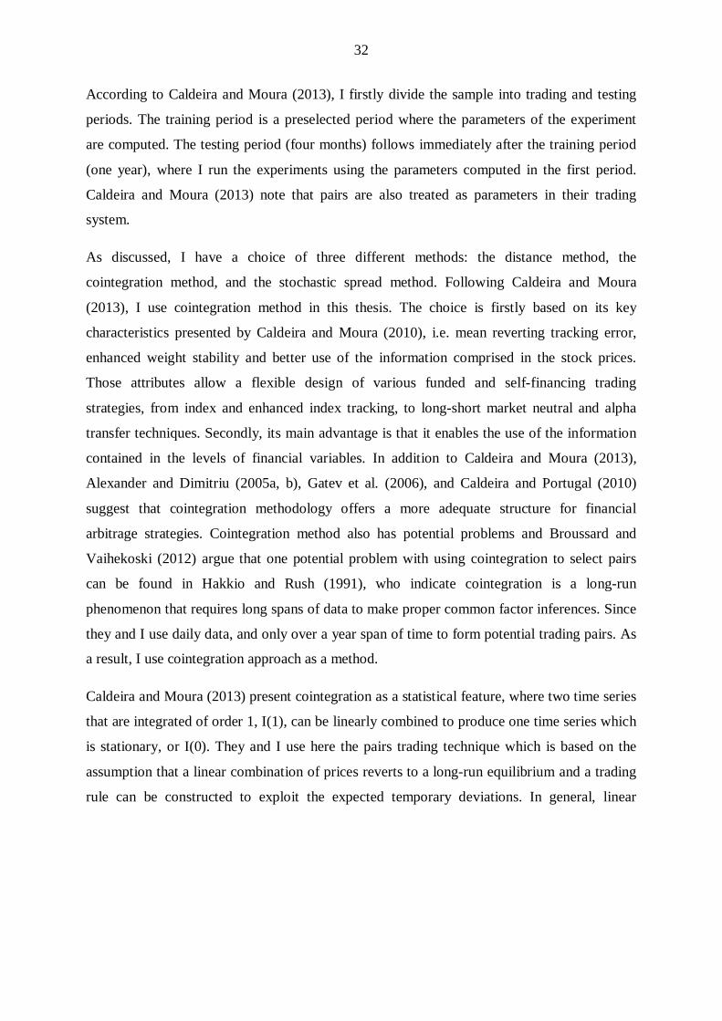
According to Caldeira and Moura (2013), I firstly divide the sample into trading and testing

periods. The training period is a preselected period where the parameters of the experiment

are computed. The testing period (four months) follows immediately after the training period

(one year), where I run the experiments using the parameters computed in the first period.

Caldeira and Moura (2013) note that pairs are also treated as parameters in their trading

system.

As discussed, I have a choice of three different methods: the distance method, the

cointegration method, and the stochastic spread method. Following Caldeira and Moura

(2013), I use cointegration method in this thesis. The choice is firstly based on its key

characteristics presented by Caldeira and Moura (2010), i.e. mean reverting tracking error,

enhanced weight stability and better use of the information comprised in the stock prices.

Those attributes allow a flexible design of various funded and self-financing trading

strategies, from index and enhanced index tracking, to long-short market neutral and alpha

transfer techniques. Secondly, its main advantage is that it enables the use of the information

contained in the levels of financial variables. In addition to Caldeira and Moura (2013),

Alexander and Dimitriu (2005a, b), Gatev et al. (2006), and Caldeira and Portugal (2010)

suggest that cointegration methodology offers a more adequate structure for financial

arbitrage strategies. Cointegration method also has potential problems and Broussard and

Vaihekoski (2012) argue that one potential problem with using cointegration to select pairs

can be found in Hakkio and Rush (1991), who indicate cointegration is a long-run

phenomenon that requires long spans of data to make proper common factor inferences. Since

they and I use daily data, and only over a year span of time to form potential trading pairs. As

a result, I use cointegration approach as a method.

Caldeira and Moura (2013) present cointegration as a statistical feature, where two time series

that are integrated of order 1, I(1), can be linearly combined to produce one time series which

is stationary, or I(0). They and I use here the pairs trading technique which is based on the

assumption that a linear combination of prices reverts to a long-run equilibrium and a trading

rule can be constructed to exploit the expected temporary deviations. In general, linear

33

combination of non-stationary time series are also non-stationary, thus not all possible pairs of

stocks cointegrate. Caldeira and Moura (2013) continue by arguing the definition

A 𝑛 𝑥 1 time series vector 𝑦𝑡 is cointegrated18 if

• each of its elements individually are non-stationary and

• there exists a non-zero vector 𝛾 such that 𝛾𝑦𝑡 is stationary.

I use the model which makes the investment strategy to be market neutral, i.e. I will hold a

long 𝑙 and a short 𝑠 position both having the same value in local currency, so ∝ 𝑃𝑡𝑙 = 𝑃𝑡𝑠.

Thus, the returns provided should not be affected by the market’s direction because this

approach eliminates net equity market exposure.

The model used by Caldeira and Moura (2013) has two parts of the pairs trading algorithm

1. Pairs selection algorithm

2. Trading signals algorithm

The first algorithm is essentially based on cointegration testing and the second creates trading

signals based on predefined investment decision rules.

(1) Pairs selection algorithm

Caldeira and Moura (2013) present the objective of the pairs selection algorithm to

identifying pairs whose linear combination exhibits a significant predictable component that

is uncorrelated with underlying movements in the market as a whole. This can be done first

by checking if all the series are integrated of the same order, I(1). I will do this by the way of

Augmented Dickey Fuller Test (ADF) which is the extended version of Dickey Fuller test19

by including extra lagged in terms of the dependent variables in order to eliminate the

problem of autocorrelation, i.e. ∆𝑌𝑡 = 𝛼 + 𝛽𝑡 + 𝛾𝑌𝑡−1 + ∑ 𝛽1∆𝑌𝑡−1𝑝𝑖=1 + 𝜀𝑡 (Mushtaq, 2011).

18 For more details about cointegration analysis, see Johansen (1995); Hamilton (1994). 19 Dickey Fuller test is a formal test of stationarity which examine the null hypothesis of an autoregressive integrated moving average (ARIMA) against stationary and alternatively. E.g. equation with constant and time trend ∆𝑌𝑡 = 𝛼 + 𝛽𝑡 + 𝛾𝑌𝑡−1 + 𝜀 and testing the hypothesis 𝐻0: 𝛾 = 0, and 𝐻1: 𝛾 < 0. The null hypothesis is tested via t-statistics by formula 𝑡 = 𝛾^−𝛾𝐻0

𝑆𝐸(𝛾^). For more details about Dickey Fuller test, see (Mushtaq, 2011).

34

Having passed the ADF test, cointegration tests are performed on all possible combination of

pairs. To test for cointegration I adopt Engle and Grangers 2-step approach and Johansen test,

following Caldeira and Moura (2013). Both the ADF test and the tests for cointegration have

been processed on MATLAB software20.

Engle and Granger (1987) provide a Representation Theorem stating that if two or more series

in 𝑦𝑡 are co-integrated, there exists an error correction representation taking the following

form:

∆𝑦𝑡 = 𝐴(𝑙)∆𝑦𝑡 + 𝛾𝑧𝑡−1 + 𝜀𝑡

where 𝛾 is a matrix of coefficient of dimension 𝑛 𝑥 𝑟 of rank 𝑟, 𝑧𝑡−1 is of dimension 𝑟 𝑥 1

based on 𝑟 ≤ 𝑛 − 1 equilibrium error relationships, 𝑧𝑡 =∝′ 𝑦𝑡21 , and 𝜀𝑡 is a stationary

multivariate disturbance. (LeSage, 1999)

LeSage (1999) also presents the Engle and Grangers 2-step approach which is used in the case

of only two series 𝑦𝑡 and 𝑥𝑡 in the mode, when it can be used to determine the co-integrating

variable that will be added to VAR model in first differences to make it an error correction

(EC) model. The first step involves a regression: 𝑦𝑡 = 𝜃 + 𝛼𝑥𝑡 + 𝑧𝑡 to determine estimates of

∝ and 𝑧𝑡. The second step carries out tests on 𝑧𝑡 to determine if it is stationary, I(0). If I find

this to be the case, the condition 𝑦𝑡 = 𝜃 + 𝛼𝑥𝑡 is interpreted as the equilibrium relationship

between the two series and the error correction model is estimated as:

∆𝑦𝑡 = −𝛾1𝑧𝑡−1 + 𝑙𝑎𝑔𝑔𝑒𝑑(∆𝑥𝑡,∆𝑦𝑡) + 𝑐1 + 𝜀1𝑡

∆𝑥𝑡 = −𝛾2𝑧𝑡−1 + 𝑙𝑎𝑔𝑔𝑒𝑑(∆𝑥𝑡,∆𝑦𝑡) + 𝑐2 + 𝜀2𝑡

where 𝑧𝑡−1 = 𝑦𝑡−1 − 𝜃 − 𝛼𝑥𝑡−1, 𝑐𝑖 are constant terms and 𝜀𝑖𝑡 denote disturbances in the

model.

Johansen’s test determines the number of cointegrating relations and also implements a

multivariate extension of the 2-step Engle and Granger procedure. I.e. the Johansen procedure

20 The functions used in the tests are available at www.spatial-econometrics.com and at the book of Chan (2009). 21 The vector 𝑦𝑡 is said to be co-integrated if there exists an 𝑛 𝑥 𝑟 matrix ∝ such that 𝑧𝑡 =∝′ 𝑦𝑡 (LeSage, 1999).

35

provides a test statistic for determining𝑟, the number of co-integrating relationships between

the 𝑛 variables in 𝑦𝑡 as well as a set of 𝑟 co-integrating vectors that can be used to construct

error correction variables for the EC model22.

(2) Trading signals algorithm

After detecting cointegrating relations, I need to follow a couple of trading rules to determine

when to open and when to close a position. Following Caldeira and Moura (2013), I calculate

first the spread between the shares as 𝜀𝑡 = 𝑃𝑡𝑙 − 𝛾𝑃𝑡𝑠, where 𝜀𝑡 is the value of the spread at

time 𝑡. Accordingly, I compute the dimensionless z-score to measure the distance to the long-

term mean in units of long-term standard deviation as 𝑧𝑡 = 𝜀𝑡−𝜇𝜀𝜎𝜀

.

I use the same basic rules as Caldeira and Moura (2013) in some parts because the similar

rules have been used in the other academic studies, too. Firstly, I open a position when the z-

score hits the 1.5 standard deviation thresholds from above or from bellow which indicates a

signal of the mispricing ETFs in terms of their relative value to each other. In the case of z-

score hits the -1.5 standard deviation threshold, the portfolio of pairs is below its long-run

equilibrium value. Thus, one should buy the portfolio, i.e. buying stock 𝑙 and selling stock 𝑠.

Contrary, if z-score hits the 1.5 standard deviation threshold from above, the portfolio of pairs

is above its long-run equilibrium value or overvalued. Thus, one should sell the portfolio

short, i.e. selling stock 𝑙 and buying stock 𝑠. Then the position is closed and z-score zero

again. Caldeira and Moura (2013) underline that in all cases opening or closing a position

means buying and selling the stocks simultaneously. These values are especially significant

when transaction costs change. For instance, at the case of rising transaction costs, it could be

useful to widen the thresholds when the number of transaction decreases.

Added to these basic rules, Caldeira and Moura (2013) use some other rules to prevent from

losing too much money in unfavorable trades. They use a stop-loss to close the position if the

ratio develops in an unfavorable way. They choose the maximum loss of 7% after having

considered the stop loss constraints of 3%, 5% and 7%, and even if giving the similar results,

22 For more details about Johansen’s test, see Johansen (1995) ; (LeSage, 1999).

36

the case of a position loses of 7% rarely come back to a positive performance. However, stop

loss constraints are not always considered in academic research. Caldeira and Moura (2013)

show examples of Elliot et al., 2005; Gatev et al., 2006; Perlin, 2009; Gatarek et al , 2011 and

Nath (2006) as an exeption that adopts a stop-loss trigger to close the position whenever the

distance widens further to hit the 5th or the 95th percentile. However, Caldeira and Moura

(2013) validate their choice of using stop loss in their study by it being fundamental in

practice to avoid large losses. Finally, they never keep a position for more than 50 days,

justifying in-sample profitability of the strategy decreasing with time and basing their in-

sample result, they present 50 days to should be enough time for the pairs to revert to

equilibrium, but also a short enough time not to lose time value. They also validate their

arguments for the rules basing totally on statistics and predetermined numbers. Schizas et al.

(2011) do not use stop-loss but they use the 20-day trading horizon and also 60-day horizon in

some parts in their study of pairs trading on international ETFs. As a result, I use the rules of

Caldeira and Moura (2013) to avoid huge losses instead of not using stop-loss as well as 50-

day trading horizon based on the past empirical results. The trading signals and rules can be

summarized as

Buy to open if 𝑧𝑡 < −1.50

Sell to open if 𝑧𝑡 > 1.50

Close short position if 𝑧𝑡 < 0.50

Close long position if 𝑧𝑡 > −0.50

Use a stop loss and close position if 𝑟𝑖𝑡𝑟𝑎𝑤 < −2.00

Close position if 𝑡𝑖 > 50

where 𝑧𝑡 is the dimensionless z-score, 𝑟𝑖𝑡𝑟𝑎𝑤 is the net return for pair i on day t, and 𝑡𝑖 is the

number of the trading days for pair i.

In the pairs selection process, I apply an approach used in the study of Caldeira and Moura

(2013) and introduced by Dunis et al. (2010). According to the approach by Dunis et al.

37

(2010), I select the pairs for trading based on the best in-sample Sharpe ratios23. Thus, I

follow Caldeira and Moura (2013) by forming the portfolio of 20 best trading pairs, i.e. the

pairs with the greatest Sharpe ratios in the in-sample simulations and use them to compose a

pairs trading portfolio to be employed out-of-sample. However, as Caldeira and Moura (2013)

note, Goetzmann et al. (2002) and Gatev et al. (2006) have shown in their studies that Sharpe

Ratios can be misleading when return distributions have negative skewness, but as in their

study this would not be a concern in my study, too, because the returns to pairs portfolios

seem to be positively skewed which, instead, would bias my Sharpe ratios downward.

After selecting 20 highest Sharpe ratio pairs, four months of pairs trading are carried out. At

the end of each trading period the position that was opened and closed, and a new trading

period ending on the last observation of the previous trading period is initiated. Now stocks

and pairs can be substituted and all parameters are re-estimated. This procedure used in the

paper of Caldeira and Moura (2013) continues in a rolling window fashion until the end of the

sample.

Calculating the returns I follow, again, Caldeira and Moura (2013). Firstly, the net return for

pair I on day t can be defined as,

𝑟𝑖𝑡𝑟𝑎𝑤 = ln �𝑃𝑡𝑙

𝑃𝑡−1𝑙� − 𝛾 ln �

𝑃𝑡𝑠

𝑃𝑡−1𝑠� + 2ln (

1− 𝐶1 + 𝐶)

where 𝑃𝑡𝑙 is the price of the ETF in which I have a long position on day 𝑡, 𝑃𝑡𝑠 is the price of

the ETF I am shorting on day 𝑡, and 𝐶 refers to transaction costs.

Secondly, Caldeira and Moura (2013) define the daily net return to a portfolio of 𝑁 pairs on

day 𝑡 as,

𝑅𝑡𝑛𝑒𝑡 = �𝑤𝑖𝑡𝑅𝑖𝑡

𝑁

𝑖=1

23 Sharpe ratio is calculated using the formula 𝑟𝑖𝑡−𝑟𝑓𝜎𝑖𝑡

, where 𝑟𝑖𝑡 is the annualized return for pair i on day t, 𝑟𝑓 is the annualized risk-free return, and 𝜎𝑖𝑡 is the annualized standard deviation for pair i on day t.

38

where 𝑤𝑖𝑡 is the weight of each pair in the portfolio (in my application is 1/N), and the

corresponding simple net return 𝑅𝑖𝑡 can be derived as,

𝑅𝑖𝑡 = 𝑒𝑟𝑖𝑡 − 1

where 𝑟𝑖𝑡 is the continuously compounded monthly return ((ln ( 𝑃𝑡𝑃𝑡−1

))24.

Finally, I should also add the transaction costs into my thesis. As presented in the subchapter

2.1.3., there are many different components to be included into the transaction costs. The

usage of the transaction costs varies a lot in the different academic papers. Some

(e.g.Engelberg et al., 2008; Do and Faff, 2010; Schizas et al., 2011; Hanson and Hall, 2012)

ignore the transaction costs totally, usually to simplify their analysis, and others (e.g. Gatev et

al., 2006; Caldeira and Moura, 2013) pay high attention to the costs gathered from the

transactions. Because the trading costs significantly affect the performance of algorithmic

trading and pairs trading, especially due to multiple or high frequency trading, I include them

into my thesis. I compared the transaction costs used in the relevant studies and as a result, I

use 0.25% per trade as my transaction cost because it is used in a paper investigating in the

international market and thus not over optimize the low transaction costs (e.g. the transaction

costs in the U.S. market which seems to have the lowest rates). It also addresses the changes

in the nine year investigation period. And because ETFs are usually priced equally with

stocks the comparison with different transaction costs between relevant studies is worthwhile.

Caldeira and Moura (2013) define the ratio consisting 0.1% of brokerage fee for each share,

plus slippage for each share (long and short) of 0.05%, and 0.2% of rental cost for short

positions (average rental cost is 2% per year per share) accounting an average 0.1% for each

share when every other trade is short selling. The following table 5 summarizes the

transaction costs used in the relevant studies

24 See more details about the derivation process from Caldeira and Moura (2013).

39

Table 5 Comparison of the transaction costs between relevant studies

Table 5 describes the transaction costs used in different studies. E.g. Caldeira and Moura (2012; 2013) use the

transaction cost of 0.25% per trade in their studies (2012) and (2013).

Note: N/A indicates that the transaction costs are not used in the study.

*An average transaction cost between 1963 and 2002

**The study does not contain empirical investigation

***The transaction costs have been used but not presented in the study

****An average transaction cost between 1963 and 2009. They apply a discount of 20% annually to the

transaction costs. E.g. Transaction costs in 1974 0.90% and in recent years less than 0.10%.

Studies Transaction cost (per trade) Gatev et al. (2006) 0.405%* Herlemont (2003) N/A**

Hong and Susmel (2003) N/A Vidyamurthy (2004) N/A**

Elliot et al. (2005) N/A** Do et al. (2006) N/A Lin et al. (2006) N/A

Papadakis and Wysocki (2007) N/A Perlin (2007; 2009) 0.1%; 0.1%

Engelberg et al. (2008) N/A Jin et al. (2008) N/A

Mudchanatongsuk et al. (2008) N/A** Bolgün et al. (2009) 0.21 %

Chan (2009) 0.05 % Huck (2010) N/A***

Do and Faff (2010; 2012) N/A; 0.34%**** Schizas et al. (2011) N/A

Broussard and Vaihekoski (2012) 0.20 % Caldeira and Moura (2012; 2013) 0.25%; 0.25%

Chiu and Wong (2012) N/A** Hanson and Hall (2012) N/A

Additionally, Caldeira and Moura (2013) use a fully invested weighting scheme, which I also

follow. They cite Broussard and Vaihekoski (2012) where argued the fully invested scheme to

be less conservative as it assumes capital is always divided between the pairs that are open.

Thus, I assume in practice each pair is given the same weight at the beginning of the trading

period. I.e. for the fully invested weighting scheme, the money from a closed pair is invested

40

in the other pairs that are open and if a pair is reopened, the money is invested back by

redistributing the investment between the pairs according to their relative weights.

Calculating the statistics, I follow the interesting statistics and these formulas by Caldeira and

Moura (2013) where the pairs trading portfolios performance are examined in the terms of the

cumulative return (𝑅𝐴), variance of returns (�̂�2), Sharpe ratio (SR) and Maximum Drawdown

(MDD)25 which are computed as,

𝑅𝐴 = 252 ∗1𝑇�𝑅𝑡

𝑇

𝑡=1

�̂�𝐴 = √252 ∗1𝑇�

(𝑅𝑡 − �̂�)2𝑇

𝑡=1

𝑆𝑅 = 𝜇̂𝜎̂, where �̂� = 1

𝑇∑ 𝑤𝑖𝑡𝑅𝑖𝑡𝑇𝑡=1

𝑀𝐷𝐷 = sup𝑡∈[0,𝑇]

� sup𝑠∈[0,𝑡]

𝑅𝑠 − 𝑅𝑡�

3.2.3. The trading strategy

My trading strategy consists of two periods: training period and trading period. Training

period, which duration is 12 months, is a formation period from which the top 20 pairs

portfolios will be formed. Firstly, I eliminate the pairs which will not meet the cointegration

requirements at the 10% significance level and then I choose top 20 pairs portfolio based on

20 pairs with highest Sharpe ratios and after that I move to trading period, which duration is

four months and which results are the returns generated with the used strategy. I.e. I first

choose the best pairs to be traded based on their performance during last year, before I start

trading these for the next four months.

25 MDD is defined as the maximum percentage drop incurred from a peak to a bottom in a certain time period (Caldeira and Moura, 2013).

41

My data consists of the time series data of 208 ETFs after the first procession from January

2004 to the end of December 2012. The first training period starts from the beginning of

January 2004 and the last from the beginning of September 2011. The first trading period

starts after the first training or formation period ends, from the beginning of January 2005 and

the last after the last training period ends, from the beginning of September 2012. The

following figure 6 shows all the formation and trading periods.

Figure 6 Formation and trading periods’ alternation

Figure 6 presents the alternation of the 12-month formation and 4-month trading periods. First, formation period

1/2005 for the first 12 months starts at the beginning of the calendar year 2004 and ends at the end of the

calendar year 2004 followed by the first trading period 1/2005 for the first 4 months starts at the beginning of the

calendar year 2005 and ends at the end of April of the calendar year 2005. The second formation period 2/2005

lasts for the end of April of the calendar year 2005, partly overlapping the first (1/2005), the third (3/2005), and

the forth (1/2006) formation periods. Second trading period 2/2005 is followed by the latest trading period of

calendar year 2005 and the trading periods never overlap. The upper figure contains the entire formation periods

from 1/2005 to 1/2009 and the partly formation periods of 2/2009 and 3/2009. The trading periods from 1/2005

to 3/2008 are presented in the upper figure. Formation periods are continuing in the lower figure from 2/2009 to

3/2012 and trading periods from 1/2009 to 3/2012. The last formation period in the sample is from September of

the calendar year 2011 to end of August of the calendar year 2012 and the last trading period for the September

of the calendar year 2012 to the end of the sample.

With the presented references, and using the discussed data and methods I present my

empirical results in the next chapter.

Formation period

3/2009

Trading period 1/2005 2/2005 3/2005 1/2006 2/2006 3/2006 1/2007 2/2007 3/2007 1/2008 2/2008 3/2008

Calendar year

Formation period

Trading period 1/2009 2/2009 3/2009 1/2010 2/2010 3/2010 1/2011 2/2011 3/2011 1/2012 2/2012 3/2012

Calendar year

2/2009

2009 2010 2011 2012

2004 2005 2006 2007 2008

1/2005 1/2006 1/2007 1/2008 2/2005 2/2006 2/2007

1/2009 2/2008

3/2005 3/2006 3/2007 3/2008

1/2010 1/2011 1/2012 2/2010 2/2011 2/2012

3/2010 3/2011 3/2012

42

4. Empirical results

In this chapter, the empirical results of this study are presented. First, in subchapter 4.1 I

present my main results related to the results of top 20 portfolios, including the output from

the cointegration tests. Subchapter 4.2 shows the empirical results by presenting the results of

the subperiod analysis. Last, in subchapter 4.3 I describe the results of the comparison to past

studies.

4.1. Main results

My main results contain both examples and summaries of whole investigation. Table 6 shows

the descriptive statistics for the top 20 pairs in the sample period from September 2005 until

the end of August 2006. Of the 21,528 possible pairs, maximum of 2,278 passed the

cointegration tests of Johansen and Engle-Granger. Of those cointegration passed pairs, 20

pairs of the greatest in-sample Sharpe ratio were selected to be used out-of-sample.

The top 20 ETF pairs were selected from the whole sample size and thus any categorization

has not been done, e.g. selecting pairs from the same sector or using any other relation in pairs

formation but cross-checking all the different combinations. However, some common

characteristics are noticeable. High returns are often generated from similar ETFs, e.g. the

similar ETF traded in two separate marketplaces. In addition, quite small amount of ETFs

present the most of the top 20 pairs.

In-sample simulations generate very high Sharpe ratios when transaction costs are not taken

into account. But it is also notable, that even if all top 20 pairs present positive Sharpe ratio

in-sample simulations, not all obtained positive return in the out-of sample trading period. For

instance, all the 20 ETFs have positive Sharpe ratio in in-sample simulations of the period

from September 2005 to the end of August 2006 but 4 of the 20 pairs showed negative result

as from -15.28% to -1.00% in the portfolio during the out-of-sample period from September

2006 to the end of December 2006. I also calculated the maximum drawdown duration, which

describes the time of the fall in days in respect to the peak of the cumulative return.

According to the almost same statistical results form as Caldeira and Moura (2013), the

results for the top 20 pairs from an example period are presented in the following table,

which is an example result table of top 20 pairs collected from one formation period (from the

beginning of September 2005 to the end of August 2006), ranking based on the best in-sample

43

Sharpe ratios, to the trading period (from the beginning of September 2006 to the end of

December 2006) out-of-sample results.

Table 6 Descriptive statistics of the pairs. Sample period 2006:09 to 2006:12.

Table 6 describes the following statistics for the top 20 pairs organized with the greatest descending Sharpe

ratios. The first two columns, “ETF 1” and “ETF 2”, describe the selected pairs; “EG (ADF)” refers to Engle-

Granger Augmented Dickey Fuller (ADF) cointegration test and “JH” refers to Johansen cointegration test for

out-of-sample period; “SR” refers to Sharpe Ratio for in-sample period; “MDD Duration(days) refers to

maximum drawdown duration in days and “Net Ret.(%)” refers to the net return for out-of-sample period.

Note: The 90% critical value for ADF is -3.08 and for Johansen test it is 10.47. Pairs have been selected using

top 20 in-sample Sharpe ratios after passing the cointegration tests. However, in out-of-sample period the pairs

not necessary pass the cointegration tests. Sharpe ratios have been calculated with 4% risk-free rate and without

transaction costs. MDD Duration(days) have been calculated related to informative statistics even if the stop loss

algorithm holds.

ETF 1 ETF 2 EG (ADF) JH (λtr) SR(in-sample) MDD Duration(days) Net Ret.(%)

Pairs

266864 14915K

-5.94 20.53 5.03 10 -1.77 266864 266866

-5.99 21.79 4.75 12 1.66

268291 13264R

-6.03 26.33 4.59 6 12.03 268291 27126W

-3.83 5.66 4.41 13 6.19

266868 14327M

-7.06 35.63 4.13 0 -1.44 268291 13699M

-3.9 5.77 4.13 6 6.76

268291 41388V

-3.23 9.55 4.08 4 2.81 13699M 27126W

-7.57 27.72 4.08 16 1.66

266866 14915K

-6.85 25.72 4.06 16 -5.10 268291 873445

-2.16 9.6 3.98 4 8.34

15110D 27553M

-5.87 24.13 3.96 8 4.02 268291 291561

-6.75 27.83 3.83 10 12.65

13264R 27126W

-4.22 5.19 3.77 56 2.19 13264R 291561

-5.68 25.07 3.63 9 -1.00

689912 292242

-2.96 5.03 3.56 15 10.15 13264R 41388V

-3.07 12.69 3.52 5 1.78

13821V 14558P

-6.77 35.92 3.45 9 0.73 292589 689912

-4.12 13.39 3.45 39 9.29

14558P 292927

-2.14 6.97 3.43 4 9.87 689915 292598

-2.81 11.01 3.32 8 1.90

44

The codes of ETFs used in the previous table 6 are downloaded from Datastream. Very often

the used top 20 pairs are similar ETFs but traded in the different marketplaces. Here, for

example, 266864 (Daiwa Exchange Traded Fund-Topix) and 14915K (Nikko Exchange

Traded Index Fund Topix) are both representing all stocks in the Tokyo Price Index but these

are traded in the different marketplaces which affects to the pricing. Secondly, 13264R

(iShares Dow Jones EURO STOXX 50 (de)) and 27126W (Lyxor Dow Jones Eurostoxx

(Milan) 50) are very similar in a same way, too. But also, here are some pairs which are more

different with their characteristics, e.g. 292589 (iShares Trust Dow Jones United States BAS

Materials) and 689912 (Select Sector Standard and Poor's Depositary Receipt Trust SBI Basic

Industries) but meet the cointegration requirements in out-of-sample, too. Instead, two other

significantly different ETF pairs (268291 (Exchange Traded Fund B1-MSCI Euro) and

873445 (iShares MSCI Canada Index), and 689912 (Select Sector Standard and Poor's

Depositary Receipt Trust SBI Basic Industries)) do no longer meet cointegration requirements

in out-of-sample.

Figure 7 presents the evolution of the z-score of residuals of an example pair iShares MDAX

(de) (13821V) against Indexchange Investment (XETRA) (14558P). These ETFs are good

examples of cointegrated, well performed, pairs because these are similar ETFs traded in the

different marketplaces. Citing Caldeira and Moura (2013), the z-score measures the distance

to equilibrium of the cointegrated residual in units of standard deviations, i.e. how far away is

a given pair from the theoretical equilibrium value associated with my model. The first graph

shows the evolution of the prices for the example ETFs and the formation and the trading

periods. The second graph shows the z-score and the thresholds for the pair of these example

ETFs.

The second graph of the figure 7 describes well how the trading strategy has been completed.

The pair is open every time its spread exceeds the thresholds. For instance in an example

graph the spread exceeds the threshold -1.5 standard deviation at point a when I buy to open.

Secondly I wait when the pairs’s spread is higher than -0.5 standard deviation, i.e. at point b,

and then I close my long position. After these opening and closing positions I have made four

transaction: at the opening buy long ETF 14558P and sell short ETF 13821V at point a, and at

the closing sell long 14558P and close short 13821V at point b. Here, duration between the

opening and closing, i.e. one operation, is one day. Points c and d show the similar operation

and points e and f show the inverse transactions, i.e. when the spread exceeds the threshold

1.5 standard deviation I open the position by selling short ETF 14558P and buying long ETF

45

13821V at point e. Thereafter, I close the position when the spread exceeds the threshold 0.5.

standard deviation at point f by closing short ETF 14558P and selling long ETF 13821V. The

duration in this operation is also one day.

Figure 7 Evolution of the ETF prices and z-scores of 14558P versus 13821V from 2005:09 to

2006:12.

Note: Normalized spread and the times when the positions are open. The pair is open every time its spread

exceeds the thresholds.

Figure 8 is again a good example of similar ETFs traded in the different marketplaces. ETF

14327M (Daiwa Exchange Traded Fund-Nikkei 225) and ETF 266868 (Nikko Exchange

Traded Index Fund 225) are cointegrated and these have another basic characteristic: very

a

b

c

d

e

f

46

high peak. Here, I open the position at point g when the spread is as high as 4.08 and I close

the position on next day at point h with the z-value of -0.78.

Figure 8 Evaluation of z-scores of 14327M versus 266868 from 2005:09 to 2006:12.

Note: Normalized spread and the times when the positions are open. The pair is open every time its spread

exceeds the thresholds.

Figure 9 presents two different results. First graph presents a pair which is highly cointegrated

and traded frequently during the examination period and second graph presents a pair which is

not cointegrated in out-of-sample and thus has no trading activity.

g

h

47

Figure 9 Evaluation of z-scores of 27126W versus 13699M from 2008:09 to 2008:12 and 27127H

versus 689915 from 2009:09 to 2009:12

The upper graph presents graphically the shifts in spreads of an example of exceptionally performed pair during

its out-of-sample period. Number in labels is an ordinal number of operation and letter whether the operation is

opening (O) or closing (C) position. E.g. “10. O” indicates tenth opening position and “10. C” indicates tenth

closing position. Two labels combined indicate that there are closing and opening positions at the same point.

E.g. “11. C & 12. O” indicates eleventh closing position and twelfth opening position.

The lower graph presents graphically the shifts in spreads of an example of poorly performed pair during its out-

of-sample period.

Note: Normalized spread and the times when the positions are open. The pair is open every time its spread

exceeds the thresholds.

48

As seen in the first graph of Figure 9, ETF 27126W (Lyxor Dow Jones Eurostoxx (Milan) 50)

and ETF 13699M (Lyxor Exchange Traded Fund Dow Jones ES 50) are highly cointegrated

generating value of -5.56 in ADF-test when the critical value at 1% significance level is -4.03.

I.e. spread is varying with regularity on the both side of the z-value of zero and, in addition,

varying is high and frequent. The graph presents high variation (z-values from -5.15 to 9.33)

as well as high frequency (23 operations, i.e. 23 opening and 23 closing positions). This

eligible cointegrated pair generated net return of 10.64% in that 4 month trading period.

Second graph of Figure 9, instead, presents an undesirable pair of ETF 27127H (iShares

Russell Mid Cap Growth Index Fund) and ETF 689915 (Consumer Discretionary Select

Sector Standard and Poor's Depositary Receipt Fund). The pair is not cointegrated in the out-

of-sample period with the value of -1.98 when the critical value at 10% significance level is -

3.09. The variation in spread is neither enough to open any single position (spread does not

exceed threshold values of -1.5 or 1.5) and thus, there is no net return in that 4 month trading

period.

Table 7 summarizes the statistics of return for the pairs’ portfolios using the full sample

period from the beginning of 2004 until the end of 2012. Following Caldeira and Moura

(2013), the profitability calculated and shown generated from this out-of-sample analysis has

already been discounted for transaction costs26. First five results in the table 7 were available

after the data mining and the rest after the out-of-sample analysis. Especially notable results

are high average annualized returns with relatively low volatility of 10.45% in annualized

terms, and a low correlation of -0.51 with the market indicate my strategy to be market neutral

as designed.

26 The cost considered is 0.25% per trade on average, summing up to 1.0% per operation including two trades in opening and two trades in closing the position. Costs related to renting ETFs sold short were considered to be 2% per year.

49

Table 7 Statistics of returns of unrestricted pairs trading strategies, from 2005:01 to 2012:12

Table 7 summarizes the statistics of my pairs trading strategy from the whole sample size and from the whole

sample period.

Note: The sample period is from January 2004 to December 2012, while the out-of-sample simulations were

performed from January 2005 to December 2012. I.e. the first 12 months of the out-of-sample are training

period and the rest 8 years are a trading period divided into the subperiods of four months. Average daily net

returns are maximum and minimum average daily net returns between single pairs.

Summary Statistics of the Pairs Trading Strategy # of observations in the sample 21528 # of days in the training window 250 # of days in the trading period 84 # of trading periods 24 # of pairs in each trading period 20 # min of cointegrated pairs in a trading period 1413 # max of cointegrated pairs in a trading period 2278 Average annualized return 41.88% Average annualized net return 27.29% Annualized volatility 10.45% Annualized Sharpe Ratio 3.55 Average largest daily net return 0.49% Average lowest daily net return -0.26% Cumulative profit 105.43% Spearman correlation coefficient -0.51 Skewness 0.85 Kurtosis 0.32 Maximum Drawdown 10.82%

Caldeira and Moura (2013) emphasize the presented maximum drawdown of the strategy,

which is a simple measure of the fall in percentage terms with respect to the peak of the

cumulative return, and can be used as a measurement of how aggressively the strategy’s

leverage can be increased. I also calculated maximum drawdown, even if I used stop-loss

algorithm in my strategy, accounting 10.82%. Skewness of 0.85 describes the returns to be

positively skewed when the standard deviation overestimates risk. Kurtosis of 0.32, instead,

describes fatter tails than would be observed in a normal distribution

I used MSCI world as my benchmark index to investigate my Hypothesis 1. Figure 10

presents the cumulative return and volatility of MSCI World index.

50

Figure 10 Cumulative return and Volatility of MSCI World Index, from 2005:01 to 2012:12.

Note: The first panel of the figure describes cumulative profit of the MSCI World index and the second panel

shows annualized volatilities.

As seen in the first panel of Figure 10 the cumulative log return of 13.51% does not exceed

my cumulative log return of 105.43% and the performance of MSCI World index is not as

smooth as I have with ETF pairs trading, accounting -54.61% drop in 2008. In addition, the

annualized mean return is only 1.69% when the pairs trading strategy generates 27.29%.

51

Second panel of Figure 10 presents the volatility of MSCI World index accounting the

average annual volatility of 8.36% which is a bit lower than in the pairs trading strategy

(10.45%). However, Kurtosis, which is sometimes referred as the “volatility of volatility”, is a

way higher (8.79) than I have with ETFs (0.32). The panel shows a high peak in 2008

volatility (14.01% annualized average) which is referred in earlier studies (e.g. Caldeira and

Moura (2013)) and also my pairs trading strategy generates highest subperiodic volatility

(17.63%) in 2008. Table 8 in the next subchapter presents the subperiodic statistics of my

trading strategy.

Calculating t-statistic27 for abnormal return of ETF pairs trading strategy generates t-value of

53.06 exceeds the value of 99% confidence interval (2.58). Thus, I can accept my Hypothesis

1, i.e. statistical pairs trading with ETFs generates positive abnormal return, at the 1%

significance level.

4.2. Subperiod analysis

According to Caldeira and Moura, I discuss the subperiod analysis in an annual level. I

present it in Table 8 which summarizes annual statistics of pairs trading strategies. The table

includes the values in the trading period from 2004 to 2012 of maximum, minimum, median

and mean returns as well as standard deviation, skewness, kurtosis, accumulating net profit

(log-return), Sharpe ratio and Maximum drawdown. I follow DeMiguel et al. (2009) to test

the statistical significance of the difference between the variances and Sharpe ratios of the

returns for pairs trading and the stationary bootstrap of Politis and Romano (1994) generating

1,000 bootstrap samples with smoothing parameter q = 0.25 as Caldeira and Moura (2013.

27 T-statistic is calculated using the standard formula of 𝑡 =𝛽�𝑗−𝛽𝑗,0

𝑆𝐸(𝛽�𝑗) where 𝑆𝐸��̂�𝑗� = 𝑠

√𝑛

52

Table 8 The P&L (in %) of the statistical arbitrage strategy for 8 years

Table 8 summarizes the out-of-sample statistics for the annual percentage net returns on portfolio of top 20 pairs

between 2005:01 and 2012:12. Max, Min, Median, Mean and Accum are maximum, minimum, median, mean

and accumulating returns in the presented years. Std, Skew, Kurt, Sharpe and MDD are standard deviation,

skewness, kurtosis, Sharpe ratio and Maximum drawdown in these years. The P-values are computed using the

stationary bootstrap of Politis and Romano (1994) generating 1,000 bootstrap samples with smoothing parameter

q = 0.25.

Note: Sharpe ratios are calculated avoiding transaction costs. MDDs have been calculated related to informative

statistics even if the stop loss algorithm holds.

Year

Max Min Median Mean Std Skew Kurt Accum Sharpe MDD 2005

10.99 6.20 9.95 8.13 5.69 0.23 0.55 7.81 3.76 2.52

(0.000)

(0.000) (0.000)

2006

12.41 7.51 11.45 10.01 7.01 3.18 1.69 9.54 3.80 4.14

(0.000)

(0.000) (0.000)

2007

20.44 8.46 14.04 13.33 8.80 0.67 1.27 12.52 3.04 5.96

(0.000)

(0.000) (0.000)

2008

64.83 39.01 59.55 53.11 17.63 0.24 -0.64 42.60 4.14 10.82

(0.000)

(0.000) (0.000)

2009

67.64 22.81 48.75 46.59 12.32 0.28 -0.97 38.25 3.77 5.69

(0.000)

(0.000) (0.000)

2010

42.15 14.95 18.75 25.34 10.43 1.01 0.44 22.58 3.31 10.29

(0.000)

(0.000) (0.000)

2011

48.89 18.78 30.08 36.11 12.78 0.92 0.56 30.83 3.27 9.89

(0.000)

(0.000) (0.000)

2012

40.79 8.21 29.36 25.70 9.92 0.27 -0.38 22.87 3.33 6.45

(0.000)

(0.000) (0.000)

All Time

67.64 6.20 27.74 27.29 10.57 0.85 0.32 105.43 3.55 10.82

The presented table shows us the profitable strategy in every year, the worst performance in

year 2005 with a mean net profit of 8.13% and volatility of 5.69%. Instead, the best

performance in year 2008 generates a net mean profit of 53.11% with volatility of 17.63%

which shows the strategy to perform especially well in economy downturn (MSCI World

Index -54.61%). This is one of the reasons why hedge funds are using pairs trading strategy of

one of their main strategies. Thus, the pairs trading strategy with ETFs seems to perform well

in every subperiods. Also skewness is positive in every year which means that standard

deviation overestimates risk. Instead, kurtosis varies from negative to positive, i.e. thicknesses

of tails vary mutually between the thicknesses of normal distribution.

53

However, the pair trading strategy is very sensitive for transaction costs. Transaction costs

vary in different marketplaces and even a small rise affects significantly to profitability due to

the characteristic of high frequent trading. Thus, my results can be too high or too low. In

addition, even if ETFs can theoretically be available to short sell, practically it is not always

easy or possible. Even the marketplaces can forbid short selling for some period as occurred

in last financial crisis. These issues should be considered when reviewing the results.

4.3. Comparative analyses

In this subchapter, I compare my results to both randomly selected pairs and the past studies.

Comparison to randomly selected pairs is the performance measurement of my trading

strategy. To check the profitability of the strategy I follow Caldeira and Moura (2013) and use

bootstrap method and the simplest comparison with a naïve trading strategy which can be

done by generating randomly trading signals and trade according to them. As Gatev et al.

(2006), I conduct a bootstrap where I compare the performance of my pairs to random pairs.

Caldeira and Moura (2013) describe the process by firstly setting the historical dates in which

the various pairs are open and in each bootstrap replacing the actual ETFs with two random

ETFs with similar prior one-day returns as the ETFs in the actual pair. As they did, I bootstrap

the entire set of trading dates 2516 times. They obtain it using the same percentage transaction

costs for both the long as the short position the net return of the naïve strategy

𝑅𝑡𝑁𝑎𝑖𝑣𝑒 = �𝑤𝑖,𝑡𝑟𝑖,𝑡 + 2𝑁𝑙𝑛 �1− 𝐶1 + 𝐶�

𝑁

𝑖=1

On average I found the mean returns of random pairs to be 1.70% annually with the Sharpe

ratio of 0.48. Which are significantly lower than the results I presented in Table 7.

In the Table 9 I compare my results to the past studies. I chose a few relevant studies to give

the brief picture of the differences of the performance between the different securities as well

as figure out whether to accept Hypothesis 2 or not. However, due to the different given

periods, the results are not fully comparable especially in an annual level but briefly show the

results of these studies.

54

Table 9 Comparison of the performances of past studies

Table 9 compares a few relevant studies by these annual percentage excess mean returns and Sharpe ratios to the

values of my study. Excess returns are calculated by using MSCI World index as benchmark index. Due to the

manners of representation the values are not fully comparable but give a brief picture of the results of the past

studies.

Sipilä (2013) Caldeira and Moura (2013) Do and Faff (2010) Schizas et al. (2011)

Year Mean Sharpe Mean Sharpe Mean Sharpe Mean Sharpe 2003

2004 2005

0.008 3.76 2003-2005

0.023 0.089

2006

-0.065 3.80 0.127 1.72 2007

0.065 3.04 0.186 2.69

2008

1.077 4.14 -0.151 0.12 2009

0.227 3.77 0.239 1.8

2006-2009:03

0.022 0.065

2003-2009

0.0288 0.831 2010

0.162 3.31 0.003 1.49

2011

0.440 3.27 -0.065 1.35 2012

0.133 3.33 0.017 1.38

All Time

0.256 3.55 0.050 1.241

As seen the excess mean returns on average are higher in my investigation. Even if the

relevant studies present higher returns in some subperiods the returns are only slightly higher

and, in addition, my returns are significantly smoother and positive. Especially years in

economic downturn seem to generate higher excess returns. Thus, I accept Hypothesis 2 at the

1% significance level (t-value of 42.70).

55

5. Discussion and conclusions

The purpose of this thesis was to investigate algorithmic pairs trading with Exchange Traded

Funds. The study was motivated by recent findings in the performance of pairs trading. In

addition, the lack of empirical investigation of pairs trading, especially with other securities

than stocks, gave me interest to investigate pairs trading with ETFs. Opportunity to use the

trading methods in a real life trading makes the results of this thesis more useful and

applicable.

The analysis was performed by following mainly the model discussed in Caldeira and Moura

(2013) but also comparing with the other studies in order to verify the relevance of the study.

Brand new and relevant study allows me to use the latest academic knowledge and this

verifies that the model is up to date. The used strategy is based on cointegration, examining

the mean-reversion of pairs. I used totally 21,528 possible pair combinations in cointegration

tests in order to identify stock pairs that share a long term equilibrium relationship. Performed

Engle and Grangers and Johansen’s tests shrunk the possible pairs into maximum of 2,278

cointegrated pairs, from each formation period were obtained. After the cointegration tests, I

calculated the standardized spread between the ETFs and I simulated trades in-sample.

Subsequently, I selected 20 pairs with highest Sharpe ratios in-sample to the top 20 portfolio

to be traded out-of-sample.

The research questions that the current study set out to answer were:

(1) Are there statistical arbitrage pairs that generate significant abnormal return?

(2) Does the usage of ETFs as statistical arbitrage pairs generate even higher

abnormal return than stocks?

And related to the research questions I generated two hypotheses

H1: Statistical pairs trading with ETFs generates positive abnormal return.

H2: Statistical pairs trading with ETFs generates higher positive abnormal returns

compared to the pairs trading with stocks.

The main findings of the study show that pairs trading with ETFs generate significant

abnormal return with low volatility from the eight year trading period. The cumulate net profit

56

is 105.43% and an annual mean of 27.29% and with volatility of 10.57%. Furthermore, the

results confirmed market neutrality with no significant correlation with MSCI World index.

The present findings are in contrast with those of Caldeira and Moura (2013) since the both

investigations generate positive abnormal return with low volatility and low correlation with

the benchmark index. Comparison to the benchmark index of MSCI World and the other

studies also validate my results since the results of comparison studies (e.g. Do and Faff

(2010); Schizas et al. (2011)) are parallels. However, comparing with Schizas et al. (2011) the

abnormal return is significantly higher due to wider repertoire of ETF pairs to the portfolio.

Thus, the findings suggest that I accept both of my hypotheses as summarizes in the following

Table 10.

Table 10 Summary of the results

The table summarizes the hypotheses and main findings related to them.

Hypotheses Empirical evidence

H1 Statistical pairs trading with ETFs generates positive abnormal return.

Strong support at the 1% significance level.

H2 Statistical pairs trading with ETFs generates higher positive abnormal returns compared to the pairs trading with stocks.

Strong support at the 1% significance level.

5.1. Suggestions for further research

This thesis fills the gap in the pairs trading investigations by introducing the algorithmic pairs

trading with ETFs first time with large sample size. However, since the data for the study was

daily data, the implications made should be considered as suggestive only between the days.

Thus, possible further studies could concentrate on pairs trading investigation with intraday

data. This could still widen the picture of hedge funds’ profitability as they are high frequency

trading. It could also be possible that profitability would be significantly higher in intraday

trading than trading only daily. Furthermore, the trading horizon could fall.

57

I started the discussion on pairs trading with different securities comparing stocks with ETFs,

but there is also a need for the investigations of pairs trading with different securities (e.g.

commodities) to a warrant more research. Due to the lack of these kinds of studies, wider

comparisons could generate huge potential for using pairs trading also out of the hedge fund

world and thus increasing the market efficiency. Finally, transaction costs play a major role in

pairs trading, therefore in-depth, up-to-date, investigation of transaction costs related to pairs

trading is needed.

58

6. References

Alexander, Carol, and Anca Dimitriu. "The cointegration alpha: Enhanced index tracking and

long-short equity market neutral strategies." (2002).

Alexander, Carol, and Anca Dimitriu. "Indexing and statistical arbitrage." The Journal of

Portfolio Management 31.2 (2005a): 50-63.

Alexander, Carol, and Anca Dimitriu. "Indexing, cointegration and equity market

regimes." International Journal of Finance & Economics 10.3 (2005b): 213-231.

Alexander, Carol, and Andreza Barbosa. “Hedging and Cross-hedging ETFs.” No. icma-

dp2007-01. Henley Business School, Reading University. (2007).

Alexander, Carol, and Andreza Barbosa. "Hedging index exchange traded funds." Journal of

Banking & Finance 32.2 (2008): 326-337.

Andrade, S., Vadim Di Pietro, and M. Seasholes. "Understanding the profitability of pairs

trading." Unpublished working paper, UC Berkeley, Northwestern University (2005).

Avellaneda, Marco, and Jeong-Hyun Lee. "Statistical arbitrage in the US equities

market." Quantitative Finance 10.7 (2010): 761-782.

Berkowitz, Stephen A., Dennis E. Logue, and Eugene A. Noser. "The total cost of

transactions on the NYSE." The Journal of Finance 43.1 (2012): 97-112.

Bolgün, Kaan Evren, Engin Kurun, and Serhat Güven. "Dynamic pairs trading strategy for the

companies listed in the Istanbul stock exchange." International Review of Applied Financial

Issues and Economics 1 (2010): 37-57.

Borowski, Krzysztof. "Exchange Traded Funds (ETFs)." Studies and Works (2006): 18.

Broussard, John Paul, and Mika Vaihekoski. "Profitability of pairs trading strategy in an

illiquid market with multiple share classes." Journal of International Financial Markets,

Institutions and Money (2012).

Caldeira, João F., and Guilherme V. Moura. "Selection of a Portfolio of Pairs Based on

Cointegration: The Brazilian Case." (2012)

59

Caldeira, João, and Guilherme Moura. "Selection of a Portfolio of Pairs Based on

Cointegration: A Statistical Arbitrage Strategy." Available at SSRN 2196391. (2013).

Caldeira, João F., and Marcelo S. Portugal. "Estratégia Long-Short, Neutra ao Mercado, e

Index Tracking Baseadas em Portfólios Cointegrados." Revista Brasileira de Finanças 8.4

(2010): 469-504.

Chan, Ernie. “Quantitative trading: how to build your own algorithmic trading business.” Vol.

430. Wiley. (2009).

Chiu, Mei Choi, and Hoi Ying Wong. "Dynamic Cointegrated Pairs Trading: Time-Consistent

Mean-Variance Strategies." (2012).

D’avolio, Gene. "The market for borrowing stock." Journal of Financial Economics 66.2

(2002): 271-306.

DeMiguel, Victor, et al. "A generalized approach to portfolio optimization: Improving

performance by constraining portfolio norms." Management Science55.5 (2009): 798-812.

Do, Binh, and Robert Faff. "Does simple pairs trading still work?." Financial Analysts

Journal 66.4 (2010): 83.

Do, Binh, and Robert Faff. "Are pairs trading profits robust to trading costs?." Journal of

Financial Research 35.2 (2012): 261-287.

Do, Binh, Robert Faff, and Kais Hamza. "A new approach to modeling and estimation for

pairs trading." Proceedings of 2006 Financial Management Association European

Conference. (2006).

Dunis, Christian L., and Richard Ho. "Cointegration portfolios of European equities for index

tracking and market neutral strategies." Journal of Asset Management 6.1 (2005): 33-52.

Dunis, Christian L., et al. "Statistical arbitrage and high-frequency data with an application to

Eurostoxx 50 equities." Liverpool Business School, Working paper (2010).

Durbin, J. and Koopman, S. “Time Series Analysis by State Space Models” Oxford University

Press. (2001).

Ehrman, Douglas S. “The handbook of pairs trading: strategies using equities, options, and

futures.” Vol. 240. Wiley. (2006).

60

Elliott, Robert J., John Van Der Hoek, and William P. Malcolm. "Pairs trading." Quantitative

Finance 5.3 (2005): 271-276.

Engelberg, Joseph, Pengjie Gao, and Ravi Jagannathan. "An anatomy of pairs trading: the role

of idiosyncratic news, common information and liquidity." Third Singapore International

Conference on Finance. (2009).

Engle, R. and Granger, C. “Co-integration and Error Correction: Representation, Estimation,

and Testing”, Econometrica, (1987) Vol. 55(2), pp. 251-276.

Eom, Cheoljun, et al. "Hurst exponent and prediction based on weak-form efficient market

hypothesis of stock markets." Physica A: Statistical Mechanics and its Applications 387.18

(2008): 4630-4636.

Ferri, Richard A. “The ETF book: all you need to know about exchange-traded funds.” Wiley.

(2008).

Gatarek, L. T., Hoogerheide, L., Van Dijk, H. K., & Verbeek, M. "A simulation-based Bayes’

procedure for robust prediction of pairs trading strategies." Tinbergen Institute Discussion

Papers (2011): 09-061.

Gatev, E., Goetzmann, W., Rouwenhorst, G., “Pairs trading: Performance of a relative value

trading arbitrage rule.” Working Paper, Yale School of Management. (1999)

Gatev, Evan, William N. Goetzmann, and K. Geert Rouwenhorst. "Pairs trading: Performance

of a relative-value arbitrage rule." Review of Financial Studies 19.3 (2006): 797-827.

Goetzmann, William, Jonathan Ingersoll, Matthew I. Spiegel, and Ivo Welch. “Sharpening

sharpe ratios.” No. w9116. National Bureau of Economic Research. (2002).

Hakkio, Craig S., and Mark Rush. "Cointegration: how short is the long run?." Journal of

International Money and Finance 10.4 (1991): 571-581.

Hamilton, James D. "Time Series Analysis Princeton University Press." Princeton, NJ (1994).

Hansen, Peter Reinhard. "A test for superior predictive ability." Journal of Business &

Economic Statistics 23.4 (2005).

Hanson, Thomas, and Joshua Hall. "Statistical Arbitrage and Robust Tests for

Cointegration." Available at SSRN 2154735 (2012).

61

Hendershott, Terrence, Charles M. Jones, and Albert J. Menkveld. "Does algorithmic trading

improve liquidity?." The Journal of Finance 66.1 (2011): 1-33.

Hendershott, Terrence, and Ryan Riordan. "Algorithmic trading and

information." Manuscript, University of California, Berkeley (2009).

Herlemont, Daniel. "Pairs trading, convergence trading, cointegration." YATS Finances &

Techonologies 5 (2003).

Hong, Gwangheon, and Raul Susmel. "Pairs-trading in the asian ADR market." (2003).

Huck, Nicolas. "Pairs trading and outranking: The multi-step-ahead forecasting

case." European Journal of Operational Research 207.3 (2010): 1702-1716.

Jin, Xiaoping, Chong Suk Yoon, and Jeff Yan. "State-space modeling of mean-reverting

spreads for pairs trading." (2008).

Johansen, Søren. "Likelihood-based inference in cointegrated vector autoregressive

models." New York (1995).

Kirkpatrick, Charles D., and Julie R. Dahlquist. Technical analysis: the complete resource for

financial market technicians. FT press. (2010).

Kissell, Robert L. "Algorithmic trading strategies." (2006).

LeSage, James P. "Applied econometrics using MATLAB." Manuscript, Dept. of Economics,

University of Toronto (1999).

Leshik, Edward, and Jane Cralle. An Introduction to Algorithmic Trading: Basic to Advanced

Strategies. Vol. 544. Wiley. (2011).

Lin, Yan-Xia, Michael McCRAE, and Chandra Gulati. "Loss protection in pairs trading

through minimum profit bounds: A cointegration approach." Advances in Decision Sciences

2006 (2006).

MacKinlay, Archie Craig, and Krishna Ramaswamy. "Index-futures arbitrage and the

behavior of stock index futures prices." Review of Financial Studies 1.2 (1988): 137-158.

Mudchanatongsuk, Supakorn, James A. Primbs, and Wilfred Wong. "Optimal pairs trading: A

stochastic control approach." American Control Conference, 2008. IEEE. (2008).

62

Mushtaq, Rizwan. "Augmented Dickey Fuller Test." (2011).

Nath, P. “High Frequency Pairs Trading with U.S Treasury Securities: Risks and Rewards for

Hedge Funds.” Working Paper Series. London Business School (2006).

Patton, Andrew J. "Are “market neutral” hedge funds really market neutral?." Review of

Financial Studies 22.7 (2009): 2495-2530.

Papadakis, George, and Peter Wysocki. "Pairs trading and accounting information." Boston

University and MIT Working Paper (2007).

Perlin, Marcelo. "M of a kind: A Multivariate Approach at Pairs Trading." Available at SSRN

952782 (2007).

Perlin, Marcelo Scherer. "Evaluation of pairs-trading strategy at the Brazilian financial

market." Journal of Derivatives & Hedge Funds 15.2 (2009): 122-136.

Politis, Dimitris N., and Joseph P. Romano. "The stationary bootstrap." Journal of the

American Statistical Association 89.428 (1994): 1303-1313.

Schizas, Panagiotis, Dimitrios Thomakos, and Tao Wang. "Pairs Trading on International

ETFs." Available at SSRN 1958546 (2011).

Vidyamurthy, Ganapathy. “Pairs Trading: quantitative methods and analysis.” Vol. 217.

Wiley. (2004).

Wang, Feng, Keren Dong, and Xiaotie Deng. "Algorithmic trading system: design and

applications." Frontiers of Computer Science in China 3.2 (2009): 235-246.

Wang, Ning. "Measuring transaction costs: an incomplete survey." Conference on

Transaction Costs organized by the Ronald Coase Institutions. Chicago. USA. (2003).

Welch, Greg, and Gary Bishop. "An introduction to the Kalman filter." (1995).

White, Halbert. "A reality check for data snooping." Econometrica 68.5 (2000): 1097-1126.

63

Appendix: List of Exchange Traded Funds

Note: Appendix contains 202 ETFs with information of names, Datastream codes and exchange places used in the investigation. 6 collinear ETFs have been deleted.

Expanded Name DS Code Exchange Allmerica Securities Trust SHBI 680435 New York Amundi Exchange Traded Fund Standard and Poor's Euro (Paris-SBF) 41388V Euronext Paris Amundi Exchange Traded Fund Standard and Poor's Europe (Milan) 350 Fund 27552R Milan Biotechnology Holders Trust 277719 Non NASDAQ OTC Broadband Holdrs Trust Depositary Receipt 286770 New York Stock Exchange (NYSE) Arca Consumer Discretionary Select Sector Standard and Poor's Depositary Receipt Fund 689915 New York Stock Exchange (NYSE) Arca Credit Suisse ETF (CH) ON SMI 290302 SIX Swiss Daiwa AM Exchange Traded Fund-Banks 15363H Tokyo Stock Exchange Daiwa Exchange Traded Fund-Nikkei 225 14327M Osaka Securities Exchange Daiwa Exchange Traded Fund-Topix 266864 Tokyo Stock Exchange ETFS Metal Securities Australia Physical Gold 26995N Australian Exchange Traded Fund B1 Ethical Euro 26829X Milan Exchange Traded Fund B1-MSCI Euro 268291 Milan Fidelity Commonwealth Trust NASDAQ Composite Index Tracking Stock 27706U NASDAQ First Trust Value Line 100 Exchange Traded Fund 27119K New York Stock Exchange (NYSE) Arca First Trust Value Line Dividend Fund 27397J New York Stock Exchange (NYSE) Arca Guggenheim Standard and Poor's 500 Equal Weight Exchange Traded Fund 26997V New York Stock Exchange (NYSE) Arca Hang Seng H-Share Index Exchange Traded Fund 28198F Hong Kong Health Care Select Sector Standard and Poor's Depositary Receipt 689913 New York Stock Exchange (NYSE) Arca Hyperion 2005 Investment Grade Opportunity Term Trust 327965 New York Indexchange Investment (XETRA) 14558P XETRA Indexchange Investment (XETRA) Tecdax ex 14558N XETRA

64

Internet Architecture Holdings Deposit Recovery 286142 New York Stock Exchange (NYSE) Arca Internet Holders Trust Depositary Receipt 274609 Non NASDAQ OTC Internet Infrastructure Holdings Deposit Recovery 286141 New York Stock Exchange (NYSE) Arca iShares Barclays 1-3 Year Treasury Bond Fund 26102F New York Stock Exchange (NYSE) Arca iShares Barclays 20 Year Treasury Bond Fund 26102J New York Stock Exchange (NYSE) Arca iShares Barclays 7-10 Year Treasury Bond Fund 26119D New York Stock Exchange (NYSE) Arca iShares Barclays Tips Bond Fund 28201L New York Stock Exchange (NYSE) Arca iShares Core Standard and Poor's 500 Exchange Traded Fund 292325 New York Stock Exchange (NYSE) Arca iShares Core Standard and Poor's Mid-Cap Exchange Traded Fund 292395 New York Stock Exchange (NYSE) Arca iShares Core Standard and Poor's Small Cap Exchange Traded Fund 292402 New York Stock Exchange (NYSE) Arca iShares Core Total United States Bond Market Exchange Traded Fund 27692V New York Stock Exchange (NYSE) Arca iShares DAX (de) 13264P Frankfurt iShares Dex Universe Bond Index Fund 289780 Toronto iShares Dow Jones (AMS) Eurostoxx 50 15110D Euronext Amsterdam iShares Dow Jones (Frankfurt) Eurostoxx 50 291561 Frankfurt iShares Dow Jones (Milan) Eurostoxx 50 27553M Milan iShares Dow Jones EURO STOXX 50 (de) 13264R Frankfurt iShares Dow Jones Eurostoxx 50 14677Q London iShares Dow Jones STOXX 50 14677R London iShares Dow Jones STOXX 50 (Milan) 27126X Milan iShares Dow Jones United States Consumer Goods Sector Services Index Fund 292605 New York Stock Exchange (NYSE) Arca iShares Dow Jones United States Consumer Services Sector Index Fund 292598 New York Stock Exchange (NYSE) Arca iShares Dow Jones United States Total Market Index Fund 292590 New York Stock Exchange (NYSE) Arca iShares Euro Corporate Bond 26885L London iShares Financial Times Stock Exchange 100 291580 London iShares MDAX (de) 13821V Frankfurt iShares MSCI Australia 873442 New York Stock Exchange (NYSE) Arca iShares MSCI Austria 873443 New York Stock Exchange (NYSE) Arca iShares MSCI Belgium Capped Investable Market Index Fund 873444 New York Stock Exchange (NYSE) Arca

65

iShares MSCI Brazil Index Fund 292927 New York Stock Exchange (NYSE) Arca iShares MSCI Canada Index 873445 New York Stock Exchange (NYSE) Arca iShares MSCI China Index Exchange Traded Fund 14828X Hong Kong iShares MSCI Eafe Index Fund CAD-Hedged 28217Q Toronto iShares MSCI Emerging Markets Index Fund 26960H New York Stock Exchange (NYSE) Arca iShares MSCI EMU Index 298993 New York Stock Exchange (NYSE) Arca iShares MSCI France 873446 New York Stock Exchange (NYSE) Arca iShares MSCI Germany 873447 New York Stock Exchange (NYSE) Arca iShares MSCI Hong Kong 873448 New York Stock Exchange (NYSE) Arca iShares MSCI Italy 873450 New York Stock Exchange (NYSE) Arca iShares MSCI Japan Index Fund 873419 New York Stock Exchange (NYSE) Arca iShares MSCI Malaysia 873418 New York Stock Exchange (NYSE) Arca iShares MSCI Mexico 873417 New York Stock Exchange (NYSE) Arca iShares MSCI Netherlands Investable Market Index Fund 873416 New York Stock Exchange (NYSE) Arca iShares MSCI Pacific ex Japan Index Fund 14729T New York Stock Exchange (NYSE) Arca iShares MSCI Singapore EWS 100 873415 New York Stock Exchange (NYSE) Arca iShares MSCI South Africa Index Fund 26775V New York Stock Exchange (NYSE) Arca iShares MSCI South Korea 292242 New York Stock Exchange (NYSE) Arca iShares MSCI Spain 873453 New York Stock Exchange (NYSE) Arca iShares MSCI Sweden 873452 New York Stock Exchange (NYSE) Arca iShares MSCI Switzerland 873451 New York Stock Exchange (NYSE) Arca iShares MSCI United Kingdom 873449 New York Stock Exchange (NYSE) Arca iShares NASDAQ Biotechnology Index Fund 13527V NASDAQ iShares Russell Mid Cap Growth Index Fund 27127H New York Stock Exchange (NYSE) Arca iShares Russell Mid Cap Index Fund 27127M New York Stock Exchange (NYSE) Arca iShares Russell Midcap Value Index Fund 15294K New York Stock Exchange (NYSE) Arca iShares Standard and Poor's 500 (Milan) 26830V Milan iShares Standard and Poor's 500 Index Fund CAD-Hedged 13912Q Toronto iShares Standard and Poor's Gssi National Resources Index Fund 14729U New York Stock Exchange (NYSE) Arca

66

iShares Standard and Poor's Gsti Semiconductor Index 14331U NASDAQ iShares Standard and Poor's Gsti Software Index Fund 14331T New York Stock Exchange (NYSE) Arca iShares Standard and Poor's Gsti Technology Index Fund 13689W New York Stock Exchange (NYSE) Arca iShares Standard and Poor's Latin America 40 Index Fund 14729V New York Stock Exchange (NYSE) Arca iShares Standard and Poor's Topix 150 Index Fund 14729W New York Stock Exchange (NYSE) Arca iShares Standard and Poor's/TSX 60 Index Fund 274910 Toronto iShares Standard and Poor's/TSX Capped Composite Index Fund 13591L Toronto iShares Standard and Poor's/TSX Capped Energy Index Fund 13708U Toronto iShares Standard and Poor's/TSX Capped Financials Index Fund 13733J Toronto iShares Standard and Poor's/TSX Capped Information Technology Index Fund 13708W Toronto iShares Standard and Poor's/TSX Capped Reit Index Fund 26392N Toronto iShares Standard and Poor's/TSX Completion Index Fund 13641X Toronto iShares Tecdax (de) 13788P Frankfurt iShares Trust Cohen and Saint RLT 13484V New York Stock Exchange (NYSE) Arca iShares Trust Dow Jones Select Dividend Index Fund 27984D New York Stock Exchange (NYSE) Arca iShares Trust Dow Jones United States BAS Materials 292589 New York Stock Exchange (NYSE) Arca iShares Trust Dow Jones United States Energy 292604 New York Stock Exchange (NYSE) Arca iShares Trust Dow Jones United States Financial Security 292401 New York Stock Exchange (NYSE) Arca iShares Trust Dow Jones United States Financial Services Composite 292603 New York Stock Exchange (NYSE) Arca iShares Trust Dow Jones United States Healthcare 292602 New York Stock Exchange (NYSE) Arca iShares Trust Dow Jones United States Industrial 292601 New York Stock Exchange (NYSE) Arca iShares Trust Dow Jones United States Real Estate Index Fund 292600 New York Stock Exchange (NYSE) Arca iShares Trust Dow Jones United States Technology Sector 292327 New York Stock Exchange (NYSE) Arca iShares Trust Dow Jones United States Telecom 292400 New York Stock Exchange (NYSE) Arca iShares Trust Dow Jones United States Utilities 292599 New York Stock Exchange (NYSE) Arca iShares Trust iBoxx Invest Top Investment Grade Corporate Bond Fund 26102C New York Stock Exchange (NYSE) Arca iShares Trust MSCI Eafe Index Fund 14442F New York Stock Exchange (NYSE) Arca iShares Trust Russel 2000 Growth Index Fund 298997 New York Stock Exchange (NYSE) Arca iShares Trust Russel 2000 Value Fund 298996 New York Stock Exchange (NYSE) Arca

67

iShares Trust Russel 3000 Growth Fund 299000 New York Stock Exchange (NYSE) Arca iShares Trust Russel 3000 Value Fund 298999 New York Stock Exchange (NYSE) Arca iShares Trust Russell 1000 Growth 292397 New York Stock Exchange (NYSE) Arca iShares Trust Russell 1000 Index 292326 New York Stock Exchange (NYSE) Arca iShares Trust Russell 1000 Value 292396 New York Stock Exchange (NYSE) Arca iShares Trust Russell 2000 Index Fund 292398 New York Stock Exchange (NYSE) Arca iShares Trust Russell 3000 292399 New York Stock Exchange (NYSE) Arca iShares Trust S&P500 / Bar Value 292394 New York Stock Exchange (NYSE) Arca iShares Trust S&P500 Growth Index Fund 292393 New York Stock Exchange (NYSE) Arca iShares Trust Standard and Poor's 100 Index 26828Q New York Stock Exchange (NYSE) Arca iShares Trust Standard and Poor's Euro Plus 299010 New York Stock Exchange (NYSE) Arca iShares Trust Standard and Poor's Global 274773 New York Stock Exchange (NYSE) Arca iShares Trust Standard and Poor's Global 100 Index 255785 New York Stock Exchange (NYSE) Arca iShares Trust Standard and Poor's Global Energy Sector Index Fund 14784J New York Stock Exchange (NYSE) Arca iShares Trust Standard and Poor's Global Financials Sector Index Fund 14784K New York Stock Exchange (NYSE) Arca iShares Trust Standard and Poor's Global Healthcare Sector Index Fund 14784L New York Stock Exchange (NYSE) Arca iShares Trust Standard and Poor's Global Information Technology Sector Index Fund 14784M New York Stock Exchange (NYSE) Arca iShares Trust Standard and Poor's Mid Capital Growth 298995 New York Stock Exchange (NYSE) Arca iShares Trust Standard and Poor's Mid Capital Value 299004 New York Stock Exchange (NYSE) Arca iShares Trust Standard and Poor's Small Capital Growth 299012 New York Stock Exchange (NYSE) Arca iShares Trust Standard and Poor's Small Capital Value 299011 New York Stock Exchange (NYSE) Arca Julius Baer MCO Global Value Merged See 36092V 698562 Frankfurt Lyxor Dow Jones (Milan) Industrial Average 27552N Milan Lyxor Dow Jones Eurostoxx (Milan) 50 27126W Milan Lyxor Dow Jones Global (Milan) Titans 50 28247H Milan Lyxor Exchange Traded Fund Bel 20 Lyxor International Asset Management 26338D Euronext Brussels Lyxor Exchange Traded Fund CAC 40 13658T Euronext Paris Lyxor Exchange Traded Fund Dow Jones ES 50 13699M Euronext Paris Lyxor Exchange Traded Fund Financial Times Stock Exchange MIB 28013P Milan

68

Lyxor NASDAQ-100 (Milan) 27552U Milan Market 2000 Holdrs Touche Remnant Depositary RCT 263796 New York Stock Exchange (NYSE) Arca Merrill Lynch and Company Retail Holders Trust 13854J Non NASDAQ OTC Naftrac 02 15421T Mexico NASDAQ 100 European (Milan) Tracker 27552P Milan Nikkei 300 Stock Index Listed Fund 141401 Tokyo Stock Exchange Nikko Exchange Traded Index Fund 225 266868 Tokyo Stock Exchange Nikko Exchange Traded Index Fund Topix 14915K Tokyo Stock Exchange Nomura AM Banks 15379P Tokyo Stock Exchange Nomura AM Exchange Traded Fund-NK225 14327N Osaka Securities Exchange Oil Service Holders Trust 13505H Non NASDAQ OTC OMXH25 Index Share Exchange Traded Fund 27462D Helsinki Pharmaceutical Holders Trust 281715 Non NASDAQ OTC Polaris Taiwan Top 50 Tracker Fund 27223X Taiwan Powershares Exchange Trust Fund Dynamic Over the Counter Portfolio 26997X New York Stock Exchange (NYSE) Arca Powershares Exchange Trust Fund Trust Dynamic Market Portfolio 26997W New York Stock Exchange (NYSE) Arca Powershares QQQ Trust Series 1 696044 NASDAQ Regional Bank Holders Trust 292699 Non NASDAQ OTC Satrix 40 Trust 280237 Johannesburg Satrix Fini 26689J Johannesburg Satrix Indi 26689N Johannesburg Sector Standard and Poor's Deposit Receipt Trust Inter Financial 689917 New York Stock Exchange (NYSE) Arca Sector Standard and Poor's Depositary Receipt Trust SBI Consumer Staples 689914 New York Stock Exchange (NYSE) Arca Sector Standard and Poor's Depositary Receipt Trust SBI Inter Industries 689918 New York Stock Exchange (NYSE) Arca Sector Standard and Poor's Depositary Receipt Trust SBI Interest Technology 699936 New York Stock Exchange (NYSE) Arca Sector Standard and Poor's Depositary Receipt Trust SBI INT-Utilities 694406 New York Stock Exchange (NYSE) Arca Select Sector Standard and Poor's Depositary Receipt Fund SHBI Energy 689916 New York Stock Exchange (NYSE) Arca Select Sector Standard and Poor's Depositary Receipt Trust SBI Basic Industries 689912 New York Stock Exchange (NYSE) Arca Semiconductor Holdrs Trust (Berlin) Depositary Receipt 296242 Berlin

69

Smarttenz 865647 New Zealand Software Holders Deposit Receipt Software 12/40 265533 Non NASDAQ OTC Standard and Poor's Depositary Receipt AEX Exchange Traded Fund 13886H Euronext Amsterdam Standard and Poor's Depositary Receipt Dow Jones Global Titans Exchange Traded Fund 265649 New York Stock Exchange (NYSE) Arca Standard and Poor's Depositary Receipt Dow Jones Industrial Avenue Exchange Traded Fund 674511 New York Stock Exchange (NYSE) Arca Standard and Poor's Depositary Receipt Dow Jones Wilshire Real Estate Investment Exchange Traded Fund 13845Q New York Stock Exchange (NYSE) Arca Standard and Poor's Depositary Receipt Dow Jones Wilshire Total Market Exchange Traded Fund 266349 New York Stock Exchange (NYSE) Arca Standard and Poor's Depositary Receipt Index Shares Funds 50 Dow Jones Eurostoxx Fund 26393C New York Stock Exchange (NYSE) Arca Standard and Poor's Depositary Receipt Index Shares Funds Dow Jones STOXX 50 Fund 26393D New York Stock Exchange (NYSE) Arca Standard and Poor's Depositary Receipt Morgan Stanley Technology Exchange Traded Fund 265650 New York Stock Exchange (NYSE) Arca Standard and Poor's Depositary Receipt Standard and Poor's 500 Exchange Traded Fund Trust 327719 New York Stock Exchange (NYSE) Arca Standard and Poor's Depositary Receipt Standard and Poor's 500 Growth Exchange Traded Fund 265639 New York Stock Exchange (NYSE) Arca Standard and Poor's Depositary Receipt Standard and Poor's 500 Value Exchange Traded Fund 265642 New York Stock Exchange (NYSE) Arca Standard and Poor's Depositary Receipt Standard and Poor's 600 Small Cap Growth Exchange Traded Fund 265648 New York Stock Exchange (NYSE) Arca Standard and Poor's Depositary Receipt Standard and Poor's 600 Small Cap Value Exchange Traded Fund 265644 New York Stock Exchange (NYSE) Arca Standard and Poor's Depositary Receipt Standard and Poor's Midcap 400 Exchange Traded Fund Trust 152675 New York Stock Exchange (NYSE) Arca Standard and Poor's Depositary Receipt Standard and Poor's/ASX 200 Fund 15154P Australian Standard and Poor's Depositary Receipt Standard and Poor's/ASX 200 Listed Property Fund 15206K Australian Standard and Poor's Depositary Receipt Standard and Poor's/ASX 50 Fund 15155C Australian Standard and Poor's Depositary Receipt Straits Times Index Exchange Traded Fund 26377N Singapore TD Standard and Poor's TSX Composite Index Fund 13601P Toronto Telecommunications Holdrs Depositary Receipt 281716 Non NASDAQ OTC Topix Exchange Traded Fund 266866 Tokyo Stock Exchange Tracker Fund of Hongkong 691916 Hong Kong Trackhedge Property 27212E Johannesburg United Bank of Switzerland Fund Management Switzerland Exchange Traded Fund SMI 28195C SIX Swiss United Bank of Switzerland-Exchange Traded Fund MSCI Japan 25500R Frankfurt Van Kampen Advantage Pennsylvania Municipal Income Trust 326879 New York Van Kampen Merritt Municipal Income Trust 519756 New York

70

Van Kampen Pennsylvania Quality Municipal Trust 546175 New York Van Kampen Strategic Sector Municipal Trust 327662 New York Vanguard Extended Market Exchange Traded Fund 28025R New York Stock Exchange (NYSE) Arca Vanguard Total Stock Market Index Fund 13917E New York Stock Exchange (NYSE) Arca Wireless Holders Trust 269931 New York Stock Exchange (NYSE) Arca Xact OMX 29281P Stockholm