Algorithm Theoretical Basis Document: GCOM-W1/AMSR2 …Algorithm Theoretical . Basis Document: GCOM-W1/AMSR2 . Snow Product . Compiled by the . GCOM-W1/AMSR2 Snow Team. Version 0.2

Satellite Products and Services Review Board

Algorithm Theoretical Basis Document:

GCOM-W1/AMSR2 Snow Product

Compiled by the GCOM-W1/AMSR2 Snow Team

Version 0.2 March 4, 2016

___________________________________

NOAA Algorithm Theoretical Basis Document

GCOM-W1/AMSR2 Snow Product Page 2 of 25

TITLE: ATBD: GCOM-W1/AMSR2 SNOW PRODUCT VERSION 0.0 AUTHORS:

Yong-Keun Lee (CIMSS/UW-Madison)

Cezar Kongoli (CICS)

Jeffrey Key (NOAA/NESDIS)



DOCUMENT HISTORY

DOCUMENT REVISION LOG

DOCUMENT TITLE: ATBD – GCOM-W1/AMSR2 SNOW PRODUCT

DOCUMENT CHANGE HISTORY

Revision No. Date Revision Originator Project Group CCR Approval #

and Date

0.1 10/26/2015 Y.-K. Lee, C. Kongoli, J. Key N/A

0.2 03/04/2016 Y.-K. Lee



LIST OF CHANGES

DOCUMENT TITLE: ATBD – GCOM-W1/AMSR2 SNOW PRODUCT

LIST OF CHANGE-AFFECTED PAGES/SECTIONS/APPENDICES

Version Number Date Changed

By Page Section Description of Change(s)



TABLE OF CONTENTS

Page LIST OF TABLES ..........................................................................................................6

LIST OF AND FIGURES ..............................................................................................7

LIST OF ACRONYMNS ...............................................................................................8

1. INTRODUCTION ....................................................................................................9

1.1. Product Overview .....................................................................................9 1.1.1. Product Description ..................................................................9 1.1.2. Product Requirements .............................................................9

1.2. Satellite Instrument Description .............................................................11

2. ALGORITHM DESCRIPTION ...............................................................................12

2.1. Processing Outline ...................................................................................12

2.2. Algorithm Input .........................................................................................13

2.3. Theoretical Description ...........................................................................13 2.3.1. Snow Covered Area..................................................................13 2.3.2. Snow Depth and SWE .............................................................14

2.4. Algorithm Output ......................................................................................16

2.5. Performance Estimates ...........................................................................17 2.5.1. Test Data Description ...............................................................17 2.5.2. Sensor Effects and Retrieval Errors .......................................17

2.6. Practical Considerations .........................................................................19 2.6.1. Numerical Computation Considerations ................................19 2.6.2. Programming and Procedural Considerations .....................19 2.6.3. Quality Assessment and Diagnostics ....................................19 2.6.4. Exception Handling ...................................................................19

2.7. Validation ...................................................................................................20

3. ASSUMPTIONS AND LIMITATIONS..................................................................24

3.1. Performance Assumptions .....................................................................24

3.2. Potential Improvements ..........................................................................24

4. REFERENCES ........................................................................................................25



LIST OF TABLES Page Table 1-1: Requirements for the NOAA GCOM-W1/AMSR2 snow cover and snow depth. . 9 Table 1-2: Requirements for the NOAA GCOM-W1/AMSR2 snow water equivalent. ........ 10 Table 1-3: Comparison of AMSR2 and AMSR-E (Imaoka et al. 2010) features. ................ 11 Table 2-1: Output structure of GCOM/AMSR2 Snow EDR ................................................. 16 Table 2-2: One day comparison of GAASP outputs with corrected and uncorrected BT and CIMSS output with uncorrected BT for Jan. 15, 2015. ..................................................... 168



LIST OF AND FIGURES Page Figure 2-1: Processing outline for AMSR2 snow property retrieval algorithm. ................... 12 Figure 2-2: Statistics of AMSR-E and AMSR2 SCA compared to 24 km IMS products. The bars above and below each point indicate descending (“D”) and ascending (“A”) orbits. Monthly SCA statistics for (a) AMSR-E and (d) AMSR2. Statistics with elevation range for (b) AMSR-E and (e) AMSR2, and statistics for forest fraction range for (c) AMSR-E and (f) AMSR2. A sample of five consecutive days of each month is selected for 10 years (Jun. 2002 – Sep. 2011) of AMSR-E and 2 years (Aug. 2012- May. 2014) of AMSR2. measurements. Statistics with elevation and forest fraction ranges used only winter months (Dec., Jan., and Feb.). ........................................................................................................ 21 Figure 2-3: Statistics of AMSR-E and AMSR2 SD as a function of elevation [(a) and (d)], forest fraction [(b) and (e)] and in-situ SD [(c) and (f)]. The bars above and below each point indicate descending (“D”) and ascending (“A”) orbits. Left panels are for AMSR-E and right panels are for AMSR2. A sample of five consecutive days (13-17) in winter months is selected for both AMSR-E and AMSR2. AMSR-E statistics is valid between Dec. 2002 and Feb. 2011 and AMSR2 statistics is valid between December 2012 and February 2014. ... 23



LIST OF ACRONYMNS AMSR2: Advanced Microwave Sounding Radiometer 2 AMSR-E: Advanced Microwave Scanning Radiometer for the Earth Observing System AMSU: Advanced Microwave Sounding Unit ARR: Algorithm Readiness Review CIMSS: Cooperative Institute for Meteorological Satellite Studies CONUS: Continental United States COOP: Cooperative Observer Program DDS: Data Distribution Server EDR: Environmental Data Record FAR: False Alarm Ratio fd: forest density ff: forest fraction FOV: Field of View GAASP: GCOM-W1 AMSR2 Algorithm Software Processor GCOM – W1: Global Change Observation Mission 1st – Water IMS: Interactive Multisensor Snow and Ice Mapping System JAXA: Japanese Aerospace Exploration Agency NWS: National Weather Service OSPO: Office of Satellite and Product Operations RMSE: Root Mean Square Error SDR: Satellite Data Record SCA: Snow Covered Area SD: Snow Depth SSM/I: Special Sensor Microwave Imager SSMIS: Special Sensor Microwave Imager/Sounder SWE: Snow Water Equivalent VCF: Vegetation Continuous Field



1. INTRODUCTION

1.1. Product Overview

1.1.1. Product Description

Snow is one of the most dynamic hydrological variables on the Earth’s surface and the cryospheric component with the largest seasonal variation in spatial extent and the satellite remote sensing is the primary tool for mapping the global distribution of snow parameters such as the snow covered area (SCA), snow depth (SD), and snow water equivalent (SWE). Advanced Microwave Sounding Radiometer 2 (AMSR2) onboard Global Change Observation Mission 1st – Water (GCOM-W1) satellite includes several microwave wave frequency which have been used for snow property retrieval using the Special Sensor Microwave Imager (SSM/I), the Special Sensor Microwave Imager/Sounder (SSMIS), the Advanced Microwave Sounding Unit (AMSU) and the Advanced Microwave Scanning Radiometer for the Earth Observing System (AMSR-E). The snow products based on AMSR2 microwave measurements include SCA, SD, and SWE. SD is calculated only over AMSR2 pixels identified as snow covered and SWE is calculated over AMSR2 pixels having valid SD values.

1.1.2. Product Requirements

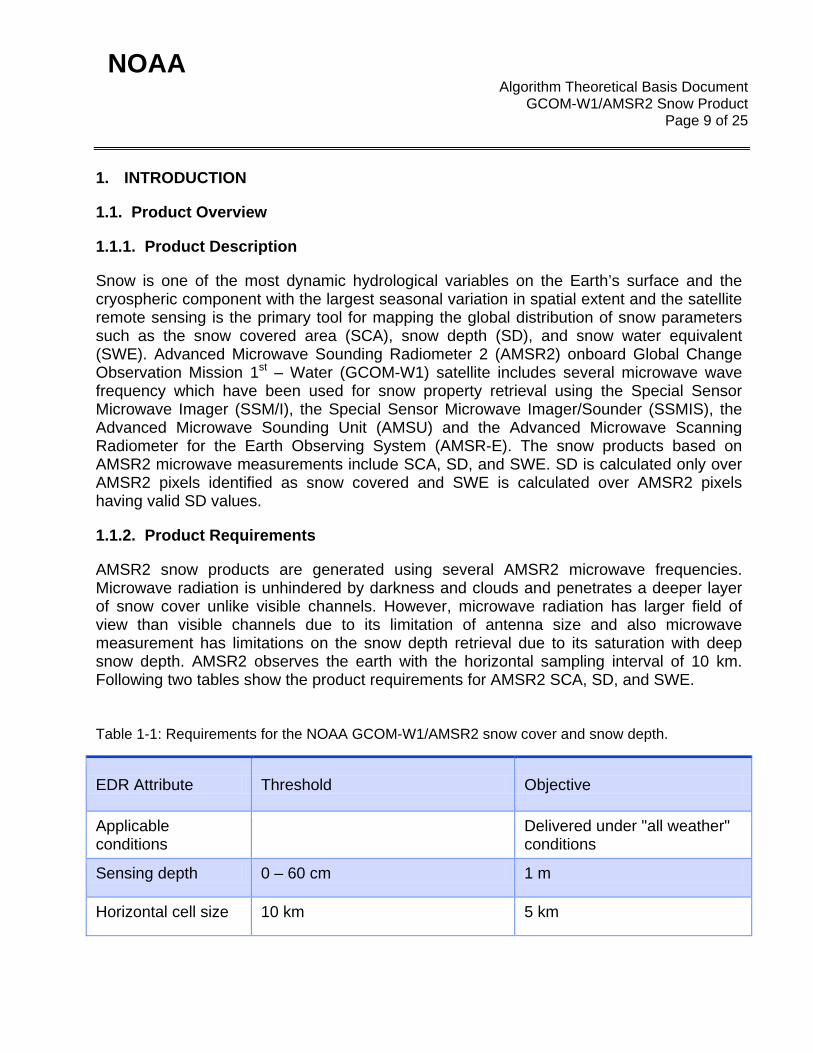
AMSR2 snow products are generated using several AMSR2 microwave frequencies. Microwave radiation is unhindered by darkness and clouds and penetrates a deeper layer of snow cover unlike visible channels. However, microwave radiation has larger field of view than visible channels due to its limitation of antenna size and also microwave measurement has limitations on the snow depth retrieval due to its saturation with deep snow depth. AMSR2 observes the earth with the horizontal sampling interval of 10 km. Following two tables show the product requirements for AMSR2 SCA, SD, and SWE. Table 1-1: Requirements for the NOAA GCOM-W1/AMSR2 snow cover and snow depth.

EDR Attribute Threshold Objective

Applicable conditions

Delivered under "all weather" conditions

Sensing depth 0 – 60 cm 1 m

Horizontal cell size 10 km 5 km



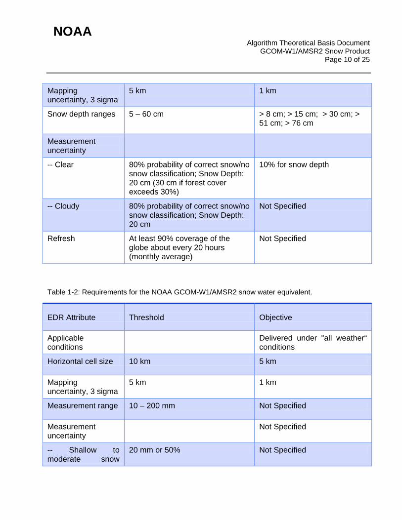
Mapping uncertainty, 3 sigma

5 km 1 km

Snow depth ranges 5 – 60 cm > 8 cm; > 15 cm; > 30 cm; > 51 cm; > 76 cm

Measurement uncertainty

-- Clear 80% probability of correct snow/no snow classification; Snow Depth: 20 cm (30 cm if forest cover exceeds 30%)

10% for snow depth

-- Cloudy 80% probability of correct snow/no snow classification; Snow Depth: 20 cm

Not Specified

Refresh At least 90% coverage of the globe about every 20 hours (monthly average)

Not Specified

Table 1-2: Requirements for the NOAA GCOM-W1/AMSR2 snow water equivalent.

EDR Attribute Threshold Objective

Applicable conditions

Delivered under "all weather“ conditions

Horizontal cell size 10 km 5 km

Mapping uncertainty, 3 sigma

5 km 1 km

Measurement range 10 – 200 mm Not Specified

Measurement uncertainty

Not Specified

-- Shallow to moderate snow

20 mm or 50% Not Specified



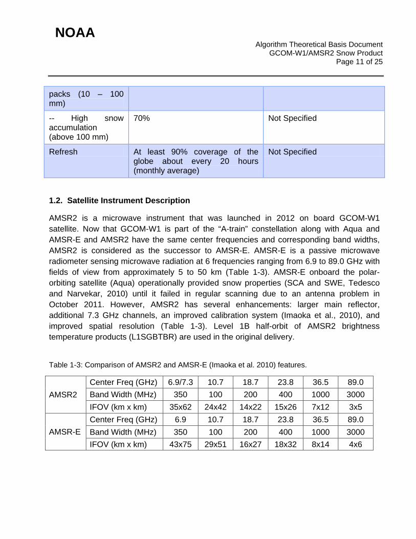
1.2. Satellite Instrument Description

AMSR2 is a microwave instrument that was launched in 2012 on board GCOM-W1 satellite. Now that GCOM-W1 is part of the “A-train” constellation along with Aqua and AMSR-E and AMSR2 have the same center frequencies and corresponding band widths, AMSR2 is considered as the successor to AMSR-E. AMSR-E is a passive microwave radiometer sensing microwave radiation at 6 frequencies ranging from 6.9 to 89.0 GHz with fields of view from approximately 5 to 50 km (Table 1-3). AMSR-E onboard the polar-orbiting satellite (Aqua) operationally provided snow properties (SCA and SWE, Tedesco and Narvekar, 2010) until it failed in regular scanning due to an antenna problem in October 2011. However, AMSR2 has several enhancements: larger main reflector, additional 7.3 GHz channels, an improved calibration system (Imaoka et al., 2010), and improved spatial resolution (Table 1-3). Level 1B half-orbit of AMSR2 brightness temperature products (L1SGBTBR) are used in the original delivery.

Table 1-3: Comparison of AMSR2 and AMSR-E (Imaoka et al. 2010) features.

AMSR2 Center Freq (GHz) 6.9/7.3 10.7 18.7 23.8 36.5 89.0 Band Width (MHz) 350 100 200 400 1000 3000 IFOV (km x km) 35x62 24x42 14x22 15x26 7x12 3x5

AMSR-E Center Freq (GHz) 6.9 10.7 18.7 23.8 36.5 89.0 Band Width (MHz) 350 100 200 400 1000 3000 IFOV (km x km) 43x75 29x51 16x27 18x32 8x14 4x6

packs (10 – 100 mm)

-- High snow accumulation (above 100 mm)

70% Not Specified

Refresh At least 90% coverage of the globe about every 20 hours (monthly average)

Not Specified



2. ALGORITHM DESCRIPTION

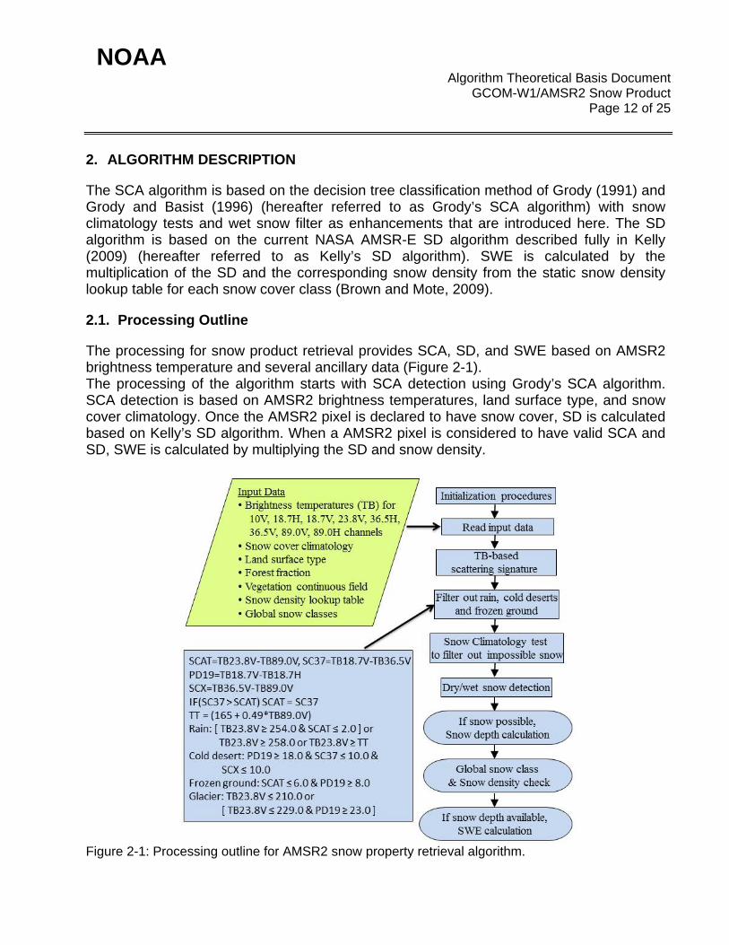
The SCA algorithm is based on the decision tree classification method of Grody (1991) and Grody and Basist (1996) (hereafter referred to as Grody’s SCA algorithm) with snow climatology tests and wet snow filter as enhancements that are introduced here. The SD algorithm is based on the current NASA AMSR-E SD algorithm described fully in Kelly (2009) (hereafter referred to as Kelly’s SD algorithm). SWE is calculated by the multiplication of the SD and the corresponding snow density from the static snow density lookup table for each snow cover class (Brown and Mote, 2009).

2.1. Processing Outline

The processing for snow product retrieval provides SCA, SD, and SWE based on AMSR2 brightness temperature and several ancillary data (Figure 2-1). The processing of the algorithm starts with SCA detection using Grody’s SCA algorithm. SCA detection is based on AMSR2 brightness temperatures, land surface type, and snow cover climatology. Once the AMSR2 pixel is declared to have snow cover, SD is calculated based on Kelly’s SD algorithm. When a AMSR2 pixel is considered to have valid SCA and SD, SWE is calculated by multiplying the SD and snow density.

Figure 2-1: Processing outline for AMSR2 snow property retrieval algorithm.



2.2. Algorithm Input

AMSR2 snow retrieval algorithm requires AMRS2 brightness temperatures between 10GHz to 89GHz at their native resolutions. The only dynamic ancillary data needed is a land surface type (land or water) which is archived with the AMSR2 brightness temperatures. Other static ancillary data include snow cover climatology, forest fraction, vegetation continuous field, snow density lookup table, and global snow cover class table. The snow cover climatology is the weekly snow frequency (probability) dataset at 1/3 degree latitude/longitude spatial resolution derived from processing NESDIS weekly snow maps available at the same resolution for the period 1973-2000 (http://www.cpc.ncep.noaa.gov/ data/snow/). Forest fraction (ff) is from the MCD12Q1 International Geosphere Biosphere Program (IGBP) classification (http://www.bu.edu/lcsc/files/2012/08/MCD12Q1_user_guide .pdf). IGBP surface type has approximately 500x500 m2 in grid cell resolution and ff is calculated by considering the pixels around the center location of an AMSR-E pixel within 7 km radius. Forest density (fd) is from the MOD44B Vegetation Continuous Field (VCF) product (http://glcf.umd.edu/library/ guide/VCF_C5_UserGuide_Dec2011.pdf). VCF has 250x250 m2 in grid cell resolution and circularly smoothed around the center location of an AMSR-E pixel within 7 km radius. The global snow classes are divided into six categories in Sturm et al. (1995); Tundra, Taiga, Maritime, Ephemeral, Prairie, and Alpine. The snow density lookup table is valid for 9 months between October and June in Brown and Mote (2009) based on the global snow cover classes.

2.3. Theoretical Description

2.3.1. Snow Covered Area

Grody’s SCA retrieval algorithm is based on a decision-tree classification method, which is described in detail in Grody (1991) and Grody and Basist (1996). Scattering surfaces (snow, deserts, rain, and frozen ground) and non-scattering surfaces (vegetation, bare soil, and water) are separated using brightness temperature-based scattering indices, followed by the application of additional brightness temperature-based thresholds to remove confounding factors (e.g., rain, frozen ground, and cold deserts). The algorithm was first applied to SMMR and SSM/I observations and later adopted for application to the Advanced Microwave Sounding Unit (AMSU) instrument (Ferraro et al., 2005; Grody et al., 2000; Kongoli et al., 2007). Figure 2-1 presents a high-level flow diagram of Grody’s SCA algorithm applied to AMSR2 data over land. An AMSR2 pixel is considered as land where the land mask is 100% at 6.9 GHz in order to minimize the water body effects. The land mask value is available as “Land_Ocean_Flag” for AMSR2 in the same file as the half-orbit Level 1B AMSR2

http://www.cpc.ncep.noaa.gov/%20data/snow/

http://www.cpc.ncep.noaa.gov/%20data/snow/

http://www.bu.edu/lcsc/files/2012/08/MCD12Q1_user_guide

http://glcf.umd.edu/library/%20guide/



brightness temperature products. The brightness temperature differences between 18.7 and 36.5 GHz and between 23.8 and 89 GHz (all vertically polarized) are used as scattering indices to separate scattering (difference is larger than 0) from non-scattering surfaces, followed by additional tests to remove warm and convective rain, cold deserts and frozen ground from the scattering surfaces indicated by the two brightness temperature differences. To further reduce errors of false snow identification, a snow climatology test has been added to Grody’s SCA algorithm. This test compares the pixels identified as snow by Grody’s SCA algorithm to a weekly snow frequency (probability) dataset at 1/3 degree latitude/longitude spatial resolution. If the probability of snow is zero, then the snow identification of the pixel is rejected and the pixel is labeled as “no-snow”. Next, a wet snow test adopted from the operational NASA AMSR-E SWE algorithm has also been added. A snow pixel is classified as “dry” when TbH36 < 245 K and TbV36 < 255 K, where TbV and TbH are vertically and horizontally polarized brightness temperatures (Tedesco and Narvekar, 2010).

2.3.2. Snow Depth and SWE

AMSR2 snow retrieval algorithm adopts the the current NASA AMSR-E SWE algorithm is based on the Kelly (2009) method of SD retrieval. Kelly’s SD algorithm calculates the dynamical coefficients relating SD to brightness temperature spectral gradients, as well as the use of a channel available on the AMSR-E instrument that is not available on SSM/I or SMMR, e.g., 10.7 GHz channel. Kelly’s SD algorithm is based on the following empirical formulation:

𝑆𝐷 (𝑐𝑚) = 𝑓𝑓 ∗ �𝑝1 ∗ (𝑇𝑏𝑉18−𝑇𝑏𝑉36)

(1−𝑓𝑑∗0.6)� +

(1 − 𝑓𝑓) ∗ [𝑝1 ∗ (𝑇𝑏𝑉10 − 𝑇𝑏𝑉36) + 𝑝2 ∗ (𝑇𝑏𝑉10 − 𝑇𝑏𝑉18)] (1) where 𝑝1 = 1

log10 (𝑇𝑏𝑉36−𝑇𝑏𝐻36) , 𝑝2 = 1

log10 (𝑇𝑏𝑉18−𝑇𝑏𝐻18) . (2)

Forest fraction (ff) and Vegetation Continuous Field (VCF) explained in Section 2.2.

In Eq. (1), SD of the forest-snow composite is computed as the sum of SD over the forest and non-forest snow components. Forested SD is computed from the brightness temperature difference at 18.7 and 36.5 GHz in proportion to the vegetation fraction ff, whereas non-forest SD is computed from both the TbV10 – TbV18 and TbV10 – TbV36 in proportion to the snow fraction (1 – ff). Use of the TbV10 – TBV18 over snow is justified by



its sensitivity to deep snow. Note that the coefficients in Eq. (1) are variable and computed from brightness temperature polarization differences (Eq. (2)). If the brightness temperature polarization difference is less than 1.1, it is set as 1.1 in Eq. (2). SD is calculated only over pixels identified as snow using Grody’s SCA algorithm. Once SD is calculated over a snow covered AMSR2 Field of View (FOV), SWE is calculated in the following way. 𝑆𝑊𝐸 = 𝑆𝐷 × 𝑠𝑛𝑜𝑤 𝑑𝑒𝑛𝑠𝑖𝑡𝑦 (3) Snow density comes from the snow density table (Brown and Mote, 2009) for each snow class (Sturm et al, 1995).



2.4. Algorithm Output

The output of the algorithm is given in Table 2-1.

Table 2-1: Output structure of GCOM/AMSR2 Snow EDR.

EDR Output Description Dynamic Range Size

Latitude Latitude of Observation Points for Low Resolution Channels -90.0 to 90.0° 243 × nscans

Longitude Longitude of Observation Points for Low Resolution Channels

-180.0 to 180.0° 243 × nscans

Snow_Cover

0: N/A 1: water 2: land without snow 3: land with wet snow possible 4: land with dry snow

[0, 1, 2, 3, 4] 243 × nscans

Snow_Depth Snow Depth 0 to 100 cm 243 × nscans

SWE Snow Water Equivalent 0 to 500kg/m2 243 × nscans

Snow_Climatology_Index

0: N/A (water) 1: no snow in climatology 2: snow in climatology but may be wet according to Tb36 (V&H) 3: snow in climatology

[0, 1, 2, 3] 243 × nscans

Snow_Depth_Index

0: no snow depth retrieval 1: no snow depth retrieval (maybe over glacier or permanent snow area) 2: land with snow, but sd or SWE exceed the limit 3: valid sd and SWE retrieval

[0, 1, 2, 3] 243 × nscans

Scattering_Surface_Index 0: N/A (water or etc.) 1: precipitation possible [0, 1, 2, …, 9] 243 × nscans



2: cold desert possible 3: rain + cold desert possible 4: frozen ground possible 5: rain + frozen ground possible 6: cold desert + frozen ground possible 7: rain + cold desert + frozen ground possible 8: glacier possible 9: valid snow cover

2.5. Performance Estimates

2.5.1. Test Data Description

10 years of AMSR-E and 2 years of AMSR2 data (SCA and SD) are used for a comprehensive analysis of performance dependencies on elevation, forest fraction, and snow depth. Since AMSR-E and AMSR2 have the same center frequencies and corresponding band widths, AMSR-E brightness temperatures are used as proxy for AMSR2. Level 2A half-orbit AMSR-E brightness temperature products (V12) are used for AMSR-E. The performance of these test datasets will be more detailed in Section 2.7. AMSR2 SWE has been compared to SNODAS SWE for one day, Jan. 15, 2015. Since GAASP provides corrected AMSR2 brightness temperature based on their truth dataset, two types of GAASP snow products are available for testing using either corrected or uncorrected AMSR2 brightness temperature.

2.5.2. Sensor Effects and Retrieval Errors

During winter, fall, and early spring, AMSR2 SCA has somewhat lower overall accuracy, snow detection rate, and omission error than AMSR-E compared to IMS. Moreover, AMSR2 has SD bias of 3.85 cm and the root mean square error (RMSE) of 20.50 cm; the descending (ascending) orbit has bias of 4.50 cm (3.04 cm) and RMSE of 21.01 cm (19.85 cm), meanwhile, AMSR-E has SD bias of 1.16 cm and RMSE of 19.90 cm; the descending (ascending) orbit shows bias of 1.81 cm (0.26 cm) and RMSE of 19.93 cm (19.86 cm). In this study, AMSR-E (winter months between December 2002 – February 2011) and AMSR2 (winter months between December 2012 – February 2014) do not have any overlapped period and thus it is not easy to say anything regarding the difference between these two instruments. Chang et al. (2012) showed that there are some differences of brightness temperatures between AMSR-E (Jun. 2002 – Jan. 2003) and AMSR2 (Jul. 2012) measurements compared to TMI. Since they showed that the brightness temperatures of AMSR-E are closer to TMI than those of AMSR2 in bias (there is no overlapped period, though), the sensor effect should be further investigated.



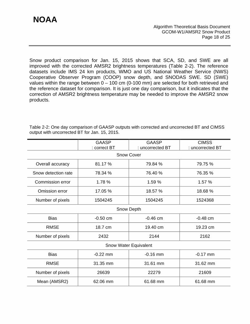
Snow product comparison for Jan. 15, 2015 shows that SCA, SD, and SWE are all improved with the corrected AMSR2 brightness temperatures (Table 2-2). The reference datasets include IMS 24 km products, WMO and US National Weather Service (NWS) Cooperative Observer Program (COOP) snow depth, and SNODAS SWE. SD (SWE) values within the range between 0 – 100 cm (0-100 mm) are selected for both retrieved and the reference dataset for comparison. It is just one day comparison, but it indicates that the correction of AMSR2 brightness temperature may be needed to improve the AMSR2 snow products.

Table 2-2: One day comparison of GAASP outputs with corrected and uncorrected BT and CIMSS output with uncorrected BT for Jan. 15, 2015.

GAASP : correct BT

GAASP : uncorrected BT

CIMSS : uncorrected BT

Snow Cover

Overall accuracy 81.17 % 79.84 % 79.75 %

Snow detection rate 78.34 % 76.40 % 76.35 %

Commission error 1.78 % 1.59 % 1.57 %

Omission error 17.05 % 18.57 % 18.68 %

Number of pixels 1504245 1504245 1524368

Snow Depth

Bias -0.50 cm -0.46 cm -0.48 cm

RMSE 18.7 cm 19.40 cm 19.23 cm

Number of pixels 2432 2144 2162

Snow Water Equivalent

Bias -0.22 mm -0.16 mm -0.17 mm

RMSE 31.35 mm 31.61 mm 31.62 mm

Number of pixels 26639 22279 21609

Mean (AMSR2) 62.06 mm 61.68 mm 61.68 mm



2.6. Practical Considerations

2.6.1. Numerical Computation Considerations

It takes less than 360 seconds for most of the half-orbit AMSR2 measurements based on the following CPU type “Intel(R) Xeon(R) CPU E5-2690 0 @ 2.90GHz”. Since the half-orbit AMSR2 brightness temperature product is generated at around 50 minute (or 3000 seconds) interval, 360 seconds is a reasonable latency to generate the snow products. If a whole-orbit is used for the snow property retrieval, the latency will be doubled.

2.6.2. Programming and Procedural Considerations

The original code of AMSR2 snow retrieval algorithm is based on Fortran 90. Ancillary data including Forest fraction (ff), Vegetation Continuous Field (VCF) and others have been prepared as static to save the huge computational burden. All the inputs including AMSR2 brightness temperatures and other ancillary data are read at the beginning of the snow product retrieval procedure. SCA is calculated first among three snow properties and then SD, and SWE is the last variable to be retrieved. Since the calculation of SD depends on SCA and the calculation of SWE depends on SD, the order of the retrieval procedure should not be changed.

2.6.3. Quality Assessment and Diagnostics

The efforts will be continued to assess the AMSR2 snow products using the reference datasets, such as IMS 24 km product, in-situ snow depth (WMO and US NWS COOP), and SWE from the data assimilated model outputs (e.g. SNODAS). The assessment can be accomplished daily since IMS 24 km products and in-situ snow depth are generated daily. IMS data and in-situ snow depth measurements are available over northern hemisphere. Although, SNODAS SWE is generated as a snap shot valid at 6 UTC each day, this can be chosen for the evaluation of satellite measured SWE due to the lack of the reference datasets of SWE. SNODAS SWE is available over the CONUS.

2.6.4. Exception Handling

The exceptional cases will be occurring, if they exist, while reading the inputs of AMSR2 brightness temperature and other ancillary data. Fatal errors within AMSR2 Brightness Temperatures may cause weird snow property retrieval but these errors are very unlikely. Since most ancillary files are static, so read errors with the ancillary data are unlikely. Once



the quality of AMSR2 Brightness Temperature data is confirmed and the computing facility is stable, the frequency of exceptional cases will be rare.

2.7. Validation

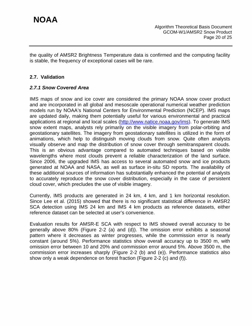
2.7.1 Snow Covered Area IMS maps of snow and ice cover are considered the primary NOAA snow cover product and are incorporated in all global and mesoscale operational numerical weather prediction models run by NOAA’s National Centers for Environmental Prediction (NCEP). IMS maps are updated daily, making them potentially useful for various environmental and practical applications at regional and local scales (http://www.natice.noaa.gov/ims). To generate IMS snow extent maps, analysts rely primarily on the visible imagery from polar-orbiting and geostationary satellites. The imagery from geostationary satellites is utilized in the form of animations, which help to distinguish moving clouds from snow. Quite often analysts visually observe and map the distribution of snow cover through semitransparent clouds. This is an obvious advantage compared to automated techniques based on visible wavelengths where most clouds prevent a reliable characterization of the land surface. Since 2006, the upgraded IMS has access to several automated snow and ice products generated at NOAA and NASA, as well as surface in-situ SD reports. The availability of these additional sources of information has substantially enhanced the potential of analysts to accurately reproduce the snow cover distribution, especially in the case of persistent cloud cover, which precludes the use of visible imagery. Currently, IMS products are generated in 24 km, 4 km, and 1 km horizontal resolution. Since Lee et al. (2015) showed that there is no significant statistical difference in AMSR2 SCA detection using IMS 24 km and IMS 4 km products as reference datasets, either reference dataset can be selected at user’s convenience. Evaluation results for AMSR-E SCA with respect to IMS showed overall accuracy to be generally above 80% (Figure 2-2 (a) and (d)). The omission error exhibits a seasonal pattern where it decreases as winter progresses, while the commission error is nearly constant (around 5%). Performance statistics show overall accuracy up to 3500 m, with omission error between 10 and 20% and commission error around 5%. Above 3500 m, the commission error increases sharply (Figure 2-2 (b) and (e)). Performance statistics also show only a weak dependence on forest fraction (Figure 2-2 (c) and (f)).

http://www.natice.noaa.gov/ims



(a) (d)

(b) (e)

(c) (f)

Figure 2-2: Statistics of AMSR-E and AMSR2 SCA compared to 24 km IMS products. The bars above and below each point indicate descending (“D”) and ascending (“A”) orbits. Monthly SCA statistics for (a) AMSR-E and (d) AMSR2. Statistics with elevation range for (b) AMSR-E and (e) AMSR2, and statistics for forest fraction range for (c) AMSR-E and (f) AMSR2. A sample of five consecutive days of each month is selected for 10 years (Jun. 2002 – Sep. 2011) of AMSR-E and 2 years (Aug. 2012- May. 2014) of AMSR2. measurements. Statistics with elevation and forest fraction ranges used only winter months (Dec., Jan., and Feb.).



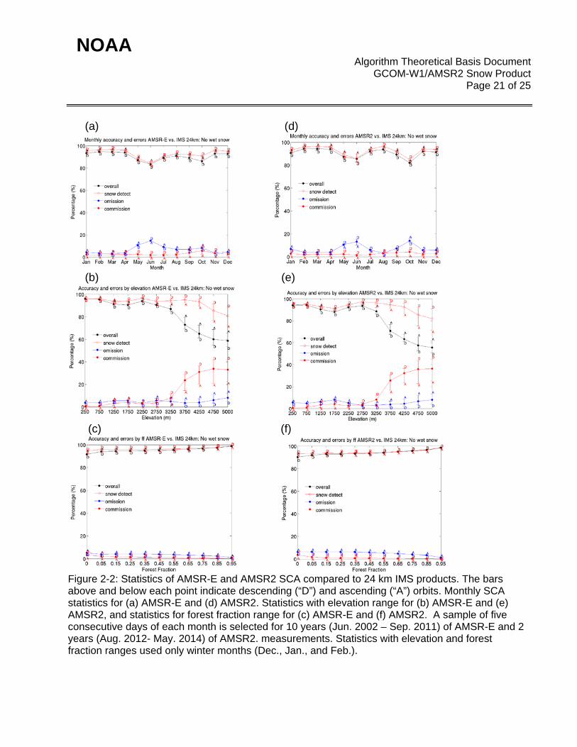
2.7.2 Snow depth AMSR-E SD error statistics (RMS error and bias) with respect to in-situ measured SD show a dependence on elevation, forest fraction, and in-situ SD (Figure 2-3). The RMSE increases with elevation, forest fraction and the magnitude of in-situ SD. Bias dependence on elevation and forest fraction were explained by the SD distribution (Lee et al., 2015). Positive bias for low-elevation and low-forest fraction areas was attributed to the predominance of shallow snow covers and the negative bias over high-elevation and high-forest fraction areas was attributed to the predominance of deeper snow covers. The AMSR2 SD comparisons to in-situ SD show similar results to those of AMSR-E, although the dependence of error statistics on elevation and forest fraction are somewhat different.



(a) (d)

(b) (e)

(c) (f)

Figure 2-3: Statistics of AMSR-E and AMSR2 SD as a function of elevation [(a) and (d)], forest fraction [(b) and (e)] and in-situ SD [(c) and (f)]. The bars above and below each point indicate descending (“D”) and ascending (“A”) orbits. Left panels are for AMSR-E and right panels are for AMSR2. A sample of five consecutive days (13-17) in winter months is selected for both AMSR-E and AMSR2. AMSR-E statistics is valid between Dec. 2002 and Feb. 2011 and AMSR2 statistics is valid between December 2012 and February 2014.



2.7.3 Snow Water Equivalent SNODAS SWE product (NOHSRC, 2004) is generated daily at around 1 km horizontal resolution but it is a snap shot valid at 06 UTC each day over CONUS. Due to the lack of the observed SWE datasets, truth dataset for SWE validation is rare. Previous studies including Tedesco and Narvekar (2010) used SNODAS SWE for their truth dataset. Since SNODAS SWE product is generated at around 1 km horizontal resolution, SNODAS pixels around the center of AMSR2 pixel can be averaged to be compared, which is not the same as the pixel to area comparison as snow depth. SWE values are selected in the range between 0 and 100 mm for both AMSR2 retrieved and SNODAS for the comparison for one month, Jan. 2015. AMSR2 SWE slightly underestimates SNODAS SWE by 0.02 mm and the RMSE value is 29.10 mm. Since Cooperative Institute for Meteorological Satellite Studies (CIMSS) is generating AMSR2 snow product daily, the archived snow products for one month Jan. 2015 at CIMSS have been used for the statistics. 3. ASSUMPTIONS AND LIMITATIONS

3.1. Performance Assumptions

Based on the investigation on the AMSR-E and AMSR2 snow products generated by the AMSR2 snow retrieval algorithm (Lee et al., 2015), the AMSR2 snow retrieval algorithm would work within the accuracy range shown in the Algorithm Readiness Review (ARR). SCA is expected to provide overall accuracy of 80 % compared to 24 km IMS products. SD is expected to provide the RMSE around 20 cm compared to in-situ snow depth measurement such as WMO and US COOP. Pixels are selected for snow depth comparison with snow depth values between 0 and 100 cm for both the retrieved and the observed. SWE is expected to provide the RMSE around 50 % of the mean AMSR2 SWE values. Pixels are selected for SWE comparison with SWE values between 0 and 100 mm for both the retrieved and the observed.

3.2. Potential Improvements

Saturation of the microwave SD signal to deeper snow remains a fundamental unresolved problem despite the use of low frequency microwave channels. However, the use of the low frequency microwave channel will be further investigated. Given the climatic controls on the regional distribution of snow cover, a reasonable strategy to improve retrieval accuracy of SD and SCA would be regional adjustment of Grody’s SCA and Kelly’s SD algorithm coefficients for use with AMSR2.



4. REFERENCES

Brown, Ross D. and Philip W. Mote. 2009. The Response of Northern Hemisphere Snow

Cover to a Changing Climate. Journal of Climate, 22, 2124–2145. Chang, P., T. King, L. Soulliard, and Z. Jelenak, 2012: GCOM-W1, AMSR2 Algorithm

Software Processor (GAASP) Package: Preliminary Design Review, Nov. 8, 2012, GAASP Preliminary Design Review.

Grody, N. C., 1991: Classification of snow cover and precipitation using the Special Sensor Microwave/Imager (SSM/I). J. Geophys. Res., 96, 7423–7435.

Grody, N. C., and A. N. Basist, 1996: Global identification of snowcover using SSM/I measurements, IEEE Trans. Geosci. Remote Sens., 34 (1), 237-249.

Imaoka, K., M. Kachi, M. Kasahara, N. Ito, K. Nakagawa, and T. Oki, 2010: Instrument Performance And Calibration Of Amsr-E And Amsr2. Proc. Int. Archives of the Photogrammetry, Remote Sensing and Spatial Information Science, vol. XXXVIII, Part 8.

Kelly, R. E., 2009: The AMSR-E Snow Depth Algorithm Description and Initial Results, J. Remote Sens. Soc. Japan, 29, No. 1 pp. 307-317.

Lee, Y.-K., J. Key, and C. Kongoli, 2015: An in-depth evaluation of heritage algorithms for snow cover and snow depth using AMSR-E and AMSR2 measurements, J. Atmos. Oceanic Technol., 32, 2319-2336, doi:10.1175/JTECH-D-15-0100.1.

National Operational Hydrologic Remote Sensing Center, 2004: Snow Data Assimilation System (SNODAS) Data Products at NSIDC. Boulder, Colorado USA: National Snow and Ice Data Center. http://dx.doi.org/10.7265/N5TB14TC.

Tedesco, M, and P. S. Narvekar, 2010: Assessment of the NASA AMSR-E SWE product, IEEE J. Sel. Top. Appl., 3, 141-159.

Sturm, M., J. Holmgren, and G. E. Liston, 1995: A seasonal snow cover classification system for local to global applications, J. Climate, 8, 1261-1283.

END OF DOCUMENT

http://dx.doi.org/10.7265/N5TB14TC.

Documents

Algorithm Theoretical Basis Document: GCOM-W1/AMSR2 …Algorithm Theoretical . Basis Document: GCOM-W1/AMSR2 . Snow Product . Compiled by the . GCOM-W1/AMSR2 Snow Team. Version 0.2