Embed Size (px)
Citation preview


SystemVue - Algorithm Design Library
1
SystemVue 2011.032011
Algorithm Design Library
This is the default Notice page

SystemVue - Algorithm Design Library
2
© Agilent Technologies, Inc. 2000-2010395 Page Mill Road, Palo Alto, CA 94304 U.S.A.No part of this manual may be reproduced in any form or by any means (includingelectronic storage and retrieval or translation into a foreign language) without prioragreement and written consent from Agilent Technologies, Inc. as governed by UnitedStates and international copyright laws.
Acknowledgments Mentor Graphics is a trademark of Mentor Graphics Corporation inthe U.S. and other countries. Microsoft®, Windows®, MS Windows®, Windows NT®, andMS-DOS® are U.S. registered trademarks of Microsoft Corporation. Pentium® is a U.S.registered trademark of Intel Corporation. PostScript® and Acrobat® are trademarks ofAdobe Systems Incorporated. UNIX® is a registered trademark of the Open Group. Java™is a U.S. trademark of Sun Microsystems, Inc. SystemC® is a registered trademark ofOpen SystemC Initiative, Inc. in the United States and other countries and is used withpermission. MATLAB® is a U.S. registered trademark of The Math Works, Inc.. HiSIM2source code, and all copyrights, trade secrets or other intellectual property rights in and tothe source code in its entirety, is owned by Hiroshima University and STARC.
Errata The SystemVue product may contain references to "HP" or "HPEESOF" such as infile names and directory names. The business entity formerly known as "HP EEsof" is nowpart of Agilent Technologies and is known as "Agilent EEsof". To avoid broken functionalityand to maintain backward compatibility for our customers, we did not change all thenames and labels that contain "HP" or "HPEESOF" references.
Warranty The material contained in this document is provided "as is", and is subject tobeing changed, without notice, in future editions. Further, to the maximum extentpermitted by applicable law, Agilent disclaims all warranties, either express or implied,with regard to this manual and any information contained herein, including but not limitedto the implied warranties of merchantability and fitness for a particular purpose. Agilentshall not be liable for errors or for incidental or consequential damages in connection withthe furnishing, use, or performance of this document or of any information containedherein. Should Agilent and the user have a separate written agreement with warrantyterms covering the material in this document that conflict with these terms, the warrantyterms in the separate agreement shall control.
Technology Licenses The hardware and/or software described in this document arefurnished under a license and may be used or copied only in accordance with the terms ofsuch license.
Portions of this product is derivative work based on the University of California PtolemySoftware System.
In no event shall the University of California be liable to any party for direct, indirect,special, incidental, or consequential damages arising out of the use of this software and itsdocumentation, even if the University of California has been advised of the possibility ofsuch damage.
The University of California specifically disclaims any warranties, including, but not limitedto, the implied warranties of merchantability and fitness for a particular purpose. Thesoftware provided hereunder is on an "as is" basis and the University of California has noobligation to provide maintenance, support, updates, enhancements, or modifications.
Portions of this product include code developed at the University of Maryland, for theseportions the following notice applies.
In no event shall the University of Maryland be liable to any party for direct, indirect,special, incidental, or consequential damages arising out of the use of this software and itsdocumentation, even if the University of Maryland has been advised of the possibility ofsuch damage.
The University of Maryland specifically disclaims any warranties, including, but not limitedto, the implied warranties of merchantability and fitness for a particular purpose. thesoftware provided hereunder is on an "as is" basis, and the University of Maryland has noobligation to provide maintenance, support, updates, enhancements, or modifications.
Portions of this product include the SystemC software licensed under Open Source terms,which are available for download at http://systemc.org/ . This software is redistributed byAgilent. The Contributors of the SystemC software provide this software "as is" and offerno warranty of any kind, express or implied, including without limitation warranties orconditions or title and non-infringement, and implied warranties or conditionsmerchantability and fitness for a particular purpose. Contributors shall not be liable forany damages of any kind including without limitation direct, indirect, special, incidentaland consequential damages, such as lost profits. Any provisions that differ from thisdisclaimer are offered by Agilent only.With respect to the portion of the Licensed Materials that describes the software andprovides instructions concerning its operation and related matters, "use" includes the rightto download and print such materials solely for the purpose described above.

SystemVue - Algorithm Design Library
3
Restricted Rights Legend If software is for use in the performance of a U.S.Government prime contract or subcontract, Software is delivered and licensed as"Commercial computer software" as defined in DFAR 252.227-7014 (June 1995), or as a"commercial item" as defined in FAR 2.101(a) or as "Restricted computer software" asdefined in FAR 52.227-19 (June 1987) or any equivalent agency regulation or contractclause. Use, duplication or disclosure of Software is subject to Agilent Technologies´standard commercial license terms, and non-DOD Departments and Agencies of the U.S.Government will receive no greater than Restricted Rights as defined in FAR 52.227-19(c)(1-2) (June 1987). U.S. Government users will receive no greater than LimitedRights as defined in FAR 52.227-14 (June 1987) or DFAR 252.227-7015 (b)(2) (November1995), as applicable in any technical data.

SystemVue - Algorithm Design Library
4
About Algorithm Design Library . . . . . . . . . . . . . . . . . . . . . . . . . . . . . . . . . . . . . . . . . . . . . . 13 Adaptive Equalizers . . . . . . . . . . . . . . . . . . . . . . . . . . . . . . . . . . . . . . . . . . . . . . . . . . . . . . 14
Contents . . . . . . . . . . . . . . . . . . . . . . . . . . . . . . . . . . . . . . . . . . . . . . . . . . . . . . . . . . . . 14 About Adaptive Equalizer Parts . . . . . . . . . . . . . . . . . . . . . . . . . . . . . . . . . . . . . . . . . . . . . . . 15
Introduction . . . . . . . . . . . . . . . . . . . . . . . . . . . . . . . . . . . . . . . . . . . . . . . . . . . . . . . . . . 15 Adaptive Filtering . . . . . . . . . . . . . . . . . . . . . . . . . . . . . . . . . . . . . . . . . . . . . . . . . . . . . . 15 Equalization . . . . . . . . . . . . . . . . . . . . . . . . . . . . . . . . . . . . . . . . . . . . . . . . . . . . . . . . . . 15 Algorithms . . . . . . . . . . . . . . . . . . . . . . . . . . . . . . . . . . . . . . . . . . . . . . . . . . . . . . . . . . . 16
AdptFltAPA_Cx Part . . . . . . . . . . . . . . . . . . . . . . . . . . . . . . . . . . . . . . . . . . . . . . . . . . . . . . . 19 AdptFltAPA_Cx . . . . . . . . . . . . . . . . . . . . . . . . . . . . . . . . . . . . . . . . . . . . . . . . . . . . . . . . . . 20 AdptFltAPA Part . . . . . . . . . . . . . . . . . . . . . . . . . . . . . . . . . . . . . . . . . . . . . . . . . . . . . . . . . 21 AdptFltAPA . . . . . . . . . . . . . . . . . . . . . . . . . . . . . . . . . . . . . . . . . . . . . . . . . . . . . . . . . . . . . 22 AdptFltCoreAPA_Cx Part . . . . . . . . . . . . . . . . . . . . . . . . . . . . . . . . . . . . . . . . . . . . . . . . . . . 23 AdptFltCoreAPA_Cx . . . . . . . . . . . . . . . . . . . . . . . . . . . . . . . . . . . . . . . . . . . . . . . . . . . . . . . 24 AdptFltCoreAPA Part . . . . . . . . . . . . . . . . . . . . . . . . . . . . . . . . . . . . . . . . . . . . . . . . . . . . . . 25 AdptFltCoreAPA . . . . . . . . . . . . . . . . . . . . . . . . . . . . . . . . . . . . . . . . . . . . . . . . . . . . . . . . . 26 AdptFltCoreLMS_Cx Part . . . . . . . . . . . . . . . . . . . . . . . . . . . . . . . . . . . . . . . . . . . . . . . . . . . 27 AdptFltCoreLMS_Cx . . . . . . . . . . . . . . . . . . . . . . . . . . . . . . . . . . . . . . . . . . . . . . . . . . . . . . 28 AdptFltCoreLMS Part . . . . . . . . . . . . . . . . . . . . . . . . . . . . . . . . . . . . . . . . . . . . . . . . . . . . . . 29 AdptFltCoreLMS . . . . . . . . . . . . . . . . . . . . . . . . . . . . . . . . . . . . . . . . . . . . . . . . . . . . . . . . . 30 AdptFltCoreRLS_Cx Part . . . . . . . . . . . . . . . . . . . . . . . . . . . . . . . . . . . . . . . . . . . . . . . . . . . 31 AdptFltCoreRLS_Cx . . . . . . . . . . . . . . . . . . . . . . . . . . . . . . . . . . . . . . . . . . . . . . . . . . . . . . . 32 AdptFltCoreRLS Part . . . . . . . . . . . . . . . . . . . . . . . . . . . . . . . . . . . . . . . . . . . . . . . . . . . . . . 33 AdptFltCoreRLS . . . . . . . . . . . . . . . . . . . . . . . . . . . . . . . . . . . . . . . . . . . . . . . . . . . . . . . . . 34 AdptFltLMS_Cx Part . . . . . . . . . . . . . . . . . . . . . . . . . . . . . . . . . . . . . . . . . . . . . . . . . . . . . . 35 AdptFltLMS_Cx . . . . . . . . . . . . . . . . . . . . . . . . . . . . . . . . . . . . . . . . . . . . . . . . . . . . . . . . . . 36 AdptFltLMS Part . . . . . . . . . . . . . . . . . . . . . . . . . . . . . . . . . . . . . . . . . . . . . . . . . . . . . . . . . 37 AdptFltLMS . . . . . . . . . . . . . . . . . . . . . . . . . . . . . . . . . . . . . . . . . . . . . . . . . . . . . . . . . . . . 38 AdptFltQR_Cx Part . . . . . . . . . . . . . . . . . . . . . . . . . . . . . . . . . . . . . . . . . . . . . . . . . . . . . . . 39 AdptFltQR_Cx . . . . . . . . . . . . . . . . . . . . . . . . . . . . . . . . . . . . . . . . . . . . . . . . . . . . . . . . . . . 40 AdptFltQR Part . . . . . . . . . . . . . . . . . . . . . . . . . . . . . . . . . . . . . . . . . . . . . . . . . . . . . . . . . . 41 AdptFltQR . . . . . . . . . . . . . . . . . . . . . . . . . . . . . . . . . . . . . . . . . . . . . . . . . . . . . . . . . . . . . 42 AdptFltRLS_Cx Part . . . . . . . . . . . . . . . . . . . . . . . . . . . . . . . . . . . . . . . . . . . . . . . . . . . . . . . 43 AdptFltRLS_Cx . . . . . . . . . . . . . . . . . . . . . . . . . . . . . . . . . . . . . . . . . . . . . . . . . . . . . . . . . . 44 AdptFltRLS Part . . . . . . . . . . . . . . . . . . . . . . . . . . . . . . . . . . . . . . . . . . . . . . . . . . . . . . . . . 45 AdptFltRLS . . . . . . . . . . . . . . . . . . . . . . . . . . . . . . . . . . . . . . . . . . . . . . . . . . . . . . . . . . . . . 46 ErrorFilterCx Part . . . . . . . . . . . . . . . . . . . . . . . . . . . . . . . . . . . . . . . . . . . . . . . . . . . . . . . . 47 ErrorFilterCx . . . . . . . . . . . . . . . . . . . . . . . . . . . . . . . . . . . . . . . . . . . . . . . . . . . . . . . . . . . 48 ErrorFilter Part . . . . . . . . . . . . . . . . . . . . . . . . . . . . . . . . . . . . . . . . . . . . . . . . . . . . . . . . . . 49 ErrorFilter . . . . . . . . . . . . . . . . . . . . . . . . . . . . . . . . . . . . . . . . . . . . . . . . . . . . . . . . . . . . . 50 LMS Part . . . . . . . . . . . . . . . . . . . . . . . . . . . . . . . . . . . . . . . . . . . . . . . . . . . . . . . . . . . . . . 51
LMS (LMS Adaptive Filter) . . . . . . . . . . . . . . . . . . . . . . . . . . . . . . . . . . . . . . . . . . . . . . . . 51 LMS_Cx (Complex LMS Adaptive Filter) . . . . . . . . . . . . . . . . . . . . . . . . . . . . . . . . . . . . . . . 51
NonLinearityCx Part . . . . . . . . . . . . . . . . . . . . . . . . . . . . . . . . . . . . . . . . . . . . . . . . . . . . . . 53 NonLinearityCx . . . . . . . . . . . . . . . . . . . . . . . . . . . . . . . . . . . . . . . . . . . . . . . . . . . . . . . . . . 54 AddEnv Part . . . . . . . . . . . . . . . . . . . . . . . . . . . . . . . . . . . . . . . . . . . . . . . . . . . . . . . . . . . . 55
AddEnv (Complex Envelope Signal Adder) . . . . . . . . . . . . . . . . . . . . . . . . . . . . . . . . . . . . . 55 AddNDensity Part . . . . . . . . . . . . . . . . . . . . . . . . . . . . . . . . . . . . . . . . . . . . . . . . . . . . . . . . 56
AddNDensity (Add Noise Density) . . . . . . . . . . . . . . . . . . . . . . . . . . . . . . . . . . . . . . . . . . . 56 AmplifierBB Part . . . . . . . . . . . . . . . . . . . . . . . . . . . . . . . . . . . . . . . . . . . . . . . . . . . . . . . . . 57
AmplifierBB (Baseband Nonlinearity With Noise Figure) . . . . . . . . . . . . . . . . . . . . . . . . . . . . 57 Amplifier Part . . . . . . . . . . . . . . . . . . . . . . . . . . . . . . . . . . . . . . . . . . . . . . . . . . . . . . . . . . . 60
Amplifier (Nonlinear Gain) . . . . . . . . . . . . . . . . . . . . . . . . . . . . . . . . . . . . . . . . . . . . . . . . 60 AtoD_ADI Part . . . . . . . . . . . . . . . . . . . . . . . . . . . . . . . . . . . . . . . . . . . . . . . . . . . . . . . . . . 64 AtoD_ADI . . . . . . . . . . . . . . . . . . . . . . . . . . . . . . . . . . . . . . . . . . . . . . . . . . . . . . . . . . . . . 65 AtoD_ADI_PMF Part . . . . . . . . . . . . . . . . . . . . . . . . . . . . . . . . . . . . . . . . . . . . . . . . . . . . . . 68 AtoD ADI PMF . . . . . . . . . . . . . . . . . . . . . . . . . . . . . . . . . . . . . . . . . . . . . . . . . . . . . . . . . . 69 AtoD_Model Part . . . . . . . . . . . . . . . . . . . . . . . . . . . . . . . . . . . . . . . . . . . . . . . . . . . . . . . . . 71
AtoD_Model . . . . . . . . . . . . . . . . . . . . . . . . . . . . . . . . . . . . . . . . . . . . . . . . . . . . . . . . . . 71 AtoD Part . . . . . . . . . . . . . . . . . . . . . . . . . . . . . . . . . . . . . . . . . . . . . . . . . . . . . . . . . . . . . . 73
AtoD . . . . . . . . . . . . . . . . . . . . . . . . . . . . . . . . . . . . . . . . . . . . . . . . . . . . . . . . . . . . . . . 73 CommsChannel Part . . . . . . . . . . . . . . . . . . . . . . . . . . . . . . . . . . . . . . . . . . . . . . . . . . . . . . 79
CommsChannel . . . . . . . . . . . . . . . . . . . . . . . . . . . . . . . . . . . . . . . . . . . . . . . . . . . . . . . . 79 CommsMIMO_Channel Part . . . . . . . . . . . . . . . . . . . . . . . . . . . . . . . . . . . . . . . . . . . . . . . . . 83
LTE_MIMO_Channel . . . . . . . . . . . . . . . . . . . . . . . . . . . . . . . . . . . . . . . . . . . . . . . . . . . . . 83 CxToEnv Part . . . . . . . . . . . . . . . . . . . . . . . . . . . . . . . . . . . . . . . . . . . . . . . . . . . . . . . . . . . 86
CxToEnv . . . . . . . . . . . . . . . . . . . . . . . . . . . . . . . . . . . . . . . . . . . . . . . . . . . . . . . . . . . . . 86 DelayEnv Part . . . . . . . . . . . . . . . . . . . . . . . . . . . . . . . . . . . . . . . . . . . . . . . . . . . . . . . . . . 87
DelayEnv . . . . . . . . . . . . . . . . . . . . . . . . . . . . . . . . . . . . . . . . . . . . . . . . . . . . . . . . . . . . 87 Demodulator Part . . . . . . . . . . . . . . . . . . . . . . . . . . . . . . . . . . . . . . . . . . . . . . . . . . . . . . . . 89
Demodulator (Demodulator) . . . . . . . . . . . . . . . . . . . . . . . . . . . . . . . . . . . . . . . . . . . . . . . 89 DownSampleEnv Part . . . . . . . . . . . . . . . . . . . . . . . . . . . . . . . . . . . . . . . . . . . . . . . . . . . . . 92
DownSampleEnv . . . . . . . . . . . . . . . . . . . . . . . . . . . . . . . . . . . . . . . . . . . . . . . . . . . . . . . 92 DtoA Part . . . . . . . . . . . . . . . . . . . . . . . . . . . . . . . . . . . . . . . . . . . . . . . . . . . . . . . . . . . . . . 94
DtoA . . . . . . . . . . . . . . . . . . . . . . . . . . . . . . . . . . . . . . . . . . . . . . . . . . . . . . . . . . . . . . . 94 EnvFcChange Part . . . . . . . . . . . . . . . . . . . . . . . . . . . . . . . . . . . . . . . . . . . . . . . . . . . . . . . . 100
EnvFcChange (Complex Envelope Signal Characterization Frequency Change) . . . . . . . . . . . . 100 EnvToCx Part . . . . . . . . . . . . . . . . . . . . . . . . . . . . . . . . . . . . . . . . . . . . . . . . . . . . . . . . . . . 101

SystemVue - Algorithm Design Library
5
EnvToCx . . . . . . . . . . . . . . . . . . . . . . . . . . . . . . . . . . . . . . . . . . . . . . . . . . . . . . . . . . . . . 101 EnvToData Part . . . . . . . . . . . . . . . . . . . . . . . . . . . . . . . . . . . . . . . . . . . . . . . . . . . . . . . . . 102
EnvToData . . . . . . . . . . . . . . . . . . . . . . . . . . . . . . . . . . . . . . . . . . . . . . . . . . . . . . . . . . . 102 FreqMpyDiv Part . . . . . . . . . . . . . . . . . . . . . . . . . . . . . . . . . . . . . . . . . . . . . . . . . . . . . . . . . 103
FreqMpyDiv . . . . . . . . . . . . . . . . . . . . . . . . . . . . . . . . . . . . . . . . . . . . . . . . . . . . . . . . . . 103 LogAmp Part . . . . . . . . . . . . . . . . . . . . . . . . . . . . . . . . . . . . . . . . . . . . . . . . . . . . . . . . . . . 105
LogAmp . . . . . . . . . . . . . . . . . . . . . . . . . . . . . . . . . . . . . . . . . . . . . . . . . . . . . . . . . . . . . 105 LogVDet Part . . . . . . . . . . . . . . . . . . . . . . . . . . . . . . . . . . . . . . . . . . . . . . . . . . . . . . . . . . . 106
LogVDet . . . . . . . . . . . . . . . . . . . . . . . . . . . . . . . . . . . . . . . . . . . . . . . . . . . . . . . . . . . . . 106 Mixer Part . . . . . . . . . . . . . . . . . . . . . . . . . . . . . . . . . . . . . . . . . . . . . . . . . . . . . . . . . . . . . 108
Mixer (Signal Mixer) . . . . . . . . . . . . . . . . . . . . . . . . . . . . . . . . . . . . . . . . . . . . . . . . . . . . 108 MpyEnv Part . . . . . . . . . . . . . . . . . . . . . . . . . . . . . . . . . . . . . . . . . . . . . . . . . . . . . . . . . . . 111
MpyEnv . . . . . . . . . . . . . . . . . . . . . . . . . . . . . . . . . . . . . . . . . . . . . . . . . . . . . . . . . . . . . 111 NoiseFMask Part . . . . . . . . . . . . . . . . . . . . . . . . . . . . . . . . . . . . . . . . . . . . . . . . . . . . . . . . . 112
NoiseFMask . . . . . . . . . . . . . . . . . . . . . . . . . . . . . . . . . . . . . . . . . . . . . . . . . . . . . . . . . . 112 Oscillator Part . . . . . . . . . . . . . . . . . . . . . . . . . . . . . . . . . . . . . . . . . . . . . . . . . . . . . . . . . . 115
Oscillator . . . . . . . . . . . . . . . . . . . . . . . . . . . . . . . . . . . . . . . . . . . . . . . . . . . . . . . . . . . . 115 PeakDetector Part . . . . . . . . . . . . . . . . . . . . . . . . . . . . . . . . . . . . . . . . . . . . . . . . . . . . . . . . 119
PeakDetector . . . . . . . . . . . . . . . . . . . . . . . . . . . . . . . . . . . . . . . . . . . . . . . . . . . . . . . . . 119 PhaseComparator Part . . . . . . . . . . . . . . . . . . . . . . . . . . . . . . . . . . . . . . . . . . . . . . . . . . . . 121
PhaseComparator . . . . . . . . . . . . . . . . . . . . . . . . . . . . . . . . . . . . . . . . . . . . . . . . . . . . . . 121 PhaseShifter Part . . . . . . . . . . . . . . . . . . . . . . . . . . . . . . . . . . . . . . . . . . . . . . . . . . . . . . . . 123
PhaseShifter . . . . . . . . . . . . . . . . . . . . . . . . . . . . . . . . . . . . . . . . . . . . . . . . . . . . . . . . . . 123 RF_Link Part . . . . . . . . . . . . . . . . . . . . . . . . . . . . . . . . . . . . . . . . . . . . . . . . . . . . . . . . . . . 124
RF_Link . . . . . . . . . . . . . . . . . . . . . . . . . . . . . . . . . . . . . . . . . . . . . . . . . . . . . . . . . . . . . 124 Overview . . . . . . . . . . . . . . . . . . . . . . . . . . . . . . . . . . . . . . . . . . . . . . . . . . . . . . . . . . . . 124 Setup UI . . . . . . . . . . . . . . . . . . . . . . . . . . . . . . . . . . . . . . . . . . . . . . . . . . . . . . . . . . . . 124 Notes/Equations . . . . . . . . . . . . . . . . . . . . . . . . . . . . . . . . . . . . . . . . . . . . . . . . . . . . . . . 125
SwitchSPDT Part . . . . . . . . . . . . . . . . . . . . . . . . . . . . . . . . . . . . . . . . . . . . . . . . . . . . . . . . . 126 SwitchSPDT . . . . . . . . . . . . . . . . . . . . . . . . . . . . . . . . . . . . . . . . . . . . . . . . . . . . . . . . . . 126
SwitchSPST Part . . . . . . . . . . . . . . . . . . . . . . . . . . . . . . . . . . . . . . . . . . . . . . . . . . . . . . . . . 129 SwitchSPST . . . . . . . . . . . . . . . . . . . . . . . . . . . . . . . . . . . . . . . . . . . . . . . . . . . . . . . . . . 129
TimeDelay Part . . . . . . . . . . . . . . . . . . . . . . . . . . . . . . . . . . . . . . . . . . . . . . . . . . . . . . . . . . 132 TimeDelay . . . . . . . . . . . . . . . . . . . . . . . . . . . . . . . . . . . . . . . . . . . . . . . . . . . . . . . . . . . 132
TimeSynchronizer Part . . . . . . . . . . . . . . . . . . . . . . . . . . . . . . . . . . . . . . . . . . . . . . . . . . . . 133 TimeSynchronizer . . . . . . . . . . . . . . . . . . . . . . . . . . . . . . . . . . . . . . . . . . . . . . . . . . . . . . 133
UpSampleEnv Part . . . . . . . . . . . . . . . . . . . . . . . . . . . . . . . . . . . . . . . . . . . . . . . . . . . . . . . 134 UpSampleEnv . . . . . . . . . . . . . . . . . . . . . . . . . . . . . . . . . . . . . . . . . . . . . . . . . . . . . . . . . 134
VCO_DivideByN Part . . . . . . . . . . . . . . . . . . . . . . . . . . . . . . . . . . . . . . . . . . . . . . . . . . . . . . 136 VCO_DivideByN . . . . . . . . . . . . . . . . . . . . . . . . . . . . . . . . . . . . . . . . . . . . . . . . . . . . . . . . 136
C++ Code Generation . . . . . . . . . . . . . . . . . . . . . . . . . . . . . . . . . . . . . . . . . . . . . . . . . . . . . 137 Contents . . . . . . . . . . . . . . . . . . . . . . . . . . . . . . . . . . . . . . . . . . . . . . . . . . . . . . . . . . . . 137
Demapper Part . . . . . . . . . . . . . . . . . . . . . . . . . . . . . . . . . . . . . . . . . . . . . . . . . . . . . . . . . . 139 Demapper (Complex Symbol Demapper) . . . . . . . . . . . . . . . . . . . . . . . . . . . . . . . . . . . . . . 139
Mapper Part . . . . . . . . . . . . . . . . . . . . . . . . . . . . . . . . . . . . . . . . . . . . . . . . . . . . . . . . . . . . 143 Mapper (Complex Symbol Mapper) . . . . . . . . . . . . . . . . . . . . . . . . . . . . . . . . . . . . . . . . . . 143
AddGuard Part . . . . . . . . . . . . . . . . . . . . . . . . . . . . . . . . . . . . . . . . . . . . . . . . . . . . . . . . . . 147 AddGuard (OFDM Symbol Guard Samples Inserter) . . . . . . . . . . . . . . . . . . . . . . . . . . . . . . . 147
BCH_Decoder Part . . . . . . . . . . . . . . . . . . . . . . . . . . . . . . . . . . . . . . . . . . . . . . . . . . . . . . . 150 BCH_Decoder . . . . . . . . . . . . . . . . . . . . . . . . . . . . . . . . . . . . . . . . . . . . . . . . . . . . . . . . . . . 151 BCH_Encoder Part . . . . . . . . . . . . . . . . . . . . . . . . . . . . . . . . . . . . . . . . . . . . . . . . . . . . . . . 154 BCH_Encoder . . . . . . . . . . . . . . . . . . . . . . . . . . . . . . . . . . . . . . . . . . . . . . . . . . . . . . . . . . . 155 CoderRS Part . . . . . . . . . . . . . . . . . . . . . . . . . . . . . . . . . . . . . . . . . . . . . . . . . . . . . . . . . . . 157
CoderRS (Reed Solomon Encoder) . . . . . . . . . . . . . . . . . . . . . . . . . . . . . . . . . . . . . . . . . . . 157 ConvolutionalCoder Part . . . . . . . . . . . . . . . . . . . . . . . . . . . . . . . . . . . . . . . . . . . . . . . . . . . 159
ConvolutionalCoder (ConvolutionalCoder) . . . . . . . . . . . . . . . . . . . . . . . . . . . . . . . . . . . . . . 159 CRC_Coder Part . . . . . . . . . . . . . . . . . . . . . . . . . . . . . . . . . . . . . . . . . . . . . . . . . . . . . . . . . 161
CRC_Coder (CRC Coder) . . . . . . . . . . . . . . . . . . . . . . . . . . . . . . . . . . . . . . . . . . . . . . . . . 161 CRC_Decoder Part . . . . . . . . . . . . . . . . . . . . . . . . . . . . . . . . . . . . . . . . . . . . . . . . . . . . . . . 163
CRC_Decoder (CRC Decoder) . . . . . . . . . . . . . . . . . . . . . . . . . . . . . . . . . . . . . . . . . . . . . . 163 DecoderRS Part . . . . . . . . . . . . . . . . . . . . . . . . . . . . . . . . . . . . . . . . . . . . . . . . . . . . . . . . . 164
DecoderRS (Reed Solomon Decoder) . . . . . . . . . . . . . . . . . . . . . . . . . . . . . . . . . . . . . . . . . 164 Deinterleaver802 Part . . . . . . . . . . . . . . . . . . . . . . . . . . . . . . . . . . . . . . . . . . . . . . . . . . . . . 167
Deinterleaver802 (IEEE 802 Deinterleaver) . . . . . . . . . . . . . . . . . . . . . . . . . . . . . . . . . . . . 167 DeScrambler Part . . . . . . . . . . . . . . . . . . . . . . . . . . . . . . . . . . . . . . . . . . . . . . . . . . . . . . . . 169
DeScrambler (Bit Sequence Descrambler) . . . . . . . . . . . . . . . . . . . . . . . . . . . . . . . . . . . . . 169 FMPulseTrain Part . . . . . . . . . . . . . . . . . . . . . . . . . . . . . . . . . . . . . . . . . . . . . . . . . . . . . . . . 170
FMPulseTrain . . . . . . . . . . . . . . . . . . . . . . . . . . . . . . . . . . . . . . . . . . . . . . . . . . . . . . . . . 170 GoldCode Part . . . . . . . . . . . . . . . . . . . . . . . . . . . . . . . . . . . . . . . . . . . . . . . . . . . . . . . . . . 171
GoldCode . . . . . . . . . . . . . . . . . . . . . . . . . . . . . . . . . . . . . . . . . . . . . . . . . . . . . . . . . . . . 171 GrayDecoder Part . . . . . . . . . . . . . . . . . . . . . . . . . . . . . . . . . . . . . . . . . . . . . . . . . . . . . . . . 174
GrayDecoder (Gray Decoder) . . . . . . . . . . . . . . . . . . . . . . . . . . . . . . . . . . . . . . . . . . . . . . 174 GrayEncoder Part . . . . . . . . . . . . . . . . . . . . . . . . . . . . . . . . . . . . . . . . . . . . . . . . . . . . . . . . 175
GrayEncoder (Gray Encoder) . . . . . . . . . . . . . . . . . . . . . . . . . . . . . . . . . . . . . . . . . . . . . . 175 InterleaveDeinterleave Part . . . . . . . . . . . . . . . . . . . . . . . . . . . . . . . . . . . . . . . . . . . . . . . . . 177
InterleaveDeinterleave (Interleaver/Deinterleaver) . . . . . . . . . . . . . . . . . . . . . . . . . . . . . . . 177 Interleaver802 Part . . . . . . . . . . . . . . . . . . . . . . . . . . . . . . . . . . . . . . . . . . . . . . . . . . . . . . . 178
Interleaver802 (IEEE 802 Interleaver) . . . . . . . . . . . . . . . . . . . . . . . . . . . . . . . . . . . . . . . . 178
SystemVue - Algorithm Design Library
6
LFSR Part . . . . . . . . . . . . . . . . . . . . . . . . . . . . . . . . . . . . . . . . . . . . . . . . . . . . . . . . . . . . . 180 LFSR . . . . . . . . . . . . . . . . . . . . . . . . . . . . . . . . . . . . . . . . . . . . . . . . . . . . . . . . . . . . . . . 180
LoadIFFTBuff802 Part . . . . . . . . . . . . . . . . . . . . . . . . . . . . . . . . . . . . . . . . . . . . . . . . . . . . . 184 LoadIFFTBuff802 (IEEE 802 IFFT Buffer Loader) . . . . . . . . . . . . . . . . . . . . . . . . . . . . . . . . . 184
Modulator Part . . . . . . . . . . . . . . . . . . . . . . . . . . . . . . . . . . . . . . . . . . . . . . . . . . . . . . . . . . 186 Modulator (Modulator) . . . . . . . . . . . . . . . . . . . . . . . . . . . . . . . . . . . . . . . . . . . . . . . . . . . 186 Notes/Equations . . . . . . . . . . . . . . . . . . . . . . . . . . . . . . . . . . . . . . . . . . . . . . . . . . . . . . . 186
M_PSK Part . . . . . . . . . . . . . . . . . . . . . . . . . . . . . . . . . . . . . . . . . . . . . . . . . . . . . . . . . . . . 189 M_PSK (Complex PSK Symbol Mapper) . . . . . . . . . . . . . . . . . . . . . . . . . . . . . . . . . . . . . . . 189
MuxOFDMSym802 Part . . . . . . . . . . . . . . . . . . . . . . . . . . . . . . . . . . . . . . . . . . . . . . . . . . . . 192 MuxOFDMSym802 (IEEE 802 OFDM Symbol Multiplexer) . . . . . . . . . . . . . . . . . . . . . . . . . . . 192
PAM_Demapper Part . . . . . . . . . . . . . . . . . . . . . . . . . . . . . . . . . . . . . . . . . . . . . . . . . . . . . . 195 PAM_Demapper (Pam Demapper) . . . . . . . . . . . . . . . . . . . . . . . . . . . . . . . . . . . . . . . . . . . 195 Notes/Equations . . . . . . . . . . . . . . . . . . . . . . . . . . . . . . . . . . . . . . . . . . . . . . . . . . . . . . . 195
PAM_Mapper Part . . . . . . . . . . . . . . . . . . . . . . . . . . . . . . . . . . . . . . . . . . . . . . . . . . . . . . . . 196 PAM_Mapper (PAM Mapper) . . . . . . . . . . . . . . . . . . . . . . . . . . . . . . . . . . . . . . . . . . . . . . . 196 Notes/Equations . . . . . . . . . . . . . . . . . . . . . . . . . . . . . . . . . . . . . . . . . . . . . . . . . . . . . . . 196
Scrambler Part . . . . . . . . . . . . . . . . . . . . . . . . . . . . . . . . . . . . . . . . . . . . . . . . . . . . . . . . . . 197 Scrambler (Bit Sequence Scrambler) . . . . . . . . . . . . . . . . . . . . . . . . . . . . . . . . . . . . . . . . . 197
ViterbiDecoder Part . . . . . . . . . . . . . . . . . . . . . . . . . . . . . . . . . . . . . . . . . . . . . . . . . . . . . . . 199 ViterbiDecoder (Viterbi Decoder for Convolutional Code) . . . . . . . . . . . . . . . . . . . . . . . . . . . 199
ADSCosimBlock Part . . . . . . . . . . . . . . . . . . . . . . . . . . . . . . . . . . . . . . . . . . . . . . . . . . . . . . 203 ADSCosimBlock . . . . . . . . . . . . . . . . . . . . . . . . . . . . . . . . . . . . . . . . . . . . . . . . . . . . . . . . 203 ADSCosimBlockCx . . . . . . . . . . . . . . . . . . . . . . . . . . . . . . . . . . . . . . . . . . . . . . . . . . . . . . 204 ADSCosimBlockEnv . . . . . . . . . . . . . . . . . . . . . . . . . . . . . . . . . . . . . . . . . . . . . . . . . . . . . 204
ADSCosimSink Part . . . . . . . . . . . . . . . . . . . . . . . . . . . . . . . . . . . . . . . . . . . . . . . . . . . . . . . 206 ADSCosimSink . . . . . . . . . . . . . . . . . . . . . . . . . . . . . . . . . . . . . . . . . . . . . . . . . . . . . . . . 206 ADSCosimSinkCx . . . . . . . . . . . . . . . . . . . . . . . . . . . . . . . . . . . . . . . . . . . . . . . . . . . . . . . 207 ADSCosimSinkEnv . . . . . . . . . . . . . . . . . . . . . . . . . . . . . . . . . . . . . . . . . . . . . . . . . . . . . . 207
FastCircuitEnvelope Part . . . . . . . . . . . . . . . . . . . . . . . . . . . . . . . . . . . . . . . . . . . . . . . . . . . 208 Fast Circuit Envelope . . . . . . . . . . . . . . . . . . . . . . . . . . . . . . . . . . . . . . . . . . . . . . . . . . . . 208 Comparison . . . . . . . . . . . . . . . . . . . . . . . . . . . . . . . . . . . . . . . . . . . . . . . . . . . . . . . . . . 208 Part Properties . . . . . . . . . . . . . . . . . . . . . . . . . . . . . . . . . . . . . . . . . . . . . . . . . . . . . . . . 209
GoldenGateCosim Part . . . . . . . . . . . . . . . . . . . . . . . . . . . . . . . . . . . . . . . . . . . . . . . . . . . . 212 GoldenGateCosim . . . . . . . . . . . . . . . . . . . . . . . . . . . . . . . . . . . . . . . . . . . . . . . . . . . . . . 212 Part Properties . . . . . . . . . . . . . . . . . . . . . . . . . . . . . . . . . . . . . . . . . . . . . . . . . . . . . . . . 212
DynamicPack_M Part . . . . . . . . . . . . . . . . . . . . . . . . . . . . . . . . . . . . . . . . . . . . . . . . . . . . . . 215 DynamicPack_M . . . . . . . . . . . . . . . . . . . . . . . . . . . . . . . . . . . . . . . . . . . . . . . . . . . . . . . 215
DynamicUnpack_M Part . . . . . . . . . . . . . . . . . . . . . . . . . . . . . . . . . . . . . . . . . . . . . . . . . . . . 216 DynamicUnpack_M . . . . . . . . . . . . . . . . . . . . . . . . . . . . . . . . . . . . . . . . . . . . . . . . . . . . . 216
Filters . . . . . . . . . . . . . . . . . . . . . . . . . . . . . . . . . . . . . . . . . . . . . . . . . . . . . . . . . . . . . . . . 217 Contents . . . . . . . . . . . . . . . . . . . . . . . . . . . . . . . . . . . . . . . . . . . . . . . . . . . . . . . . . . . . 217
BiquadCascade Part . . . . . . . . . . . . . . . . . . . . . . . . . . . . . . . . . . . . . . . . . . . . . . . . . . . . . . 218 BiquadCascade (IIR Filter with Cascaded Biquad Sections) . . . . . . . . . . . . . . . . . . . . . . . . . . 218
Biquad Part . . . . . . . . . . . . . . . . . . . . . . . . . . . . . . . . . . . . . . . . . . . . . . . . . . . . . . . . . . . . 219 Biquad (Biquad IIR Filter) . . . . . . . . . . . . . . . . . . . . . . . . . . . . . . . . . . . . . . . . . . . . . . . . . 219
BlockAllPole Part . . . . . . . . . . . . . . . . . . . . . . . . . . . . . . . . . . . . . . . . . . . . . . . . . . . . . . . . . 221 BlockAllPole (All-Pole Filter for Data Blocks) . . . . . . . . . . . . . . . . . . . . . . . . . . . . . . . . . . . . 221
BlockFIR Part . . . . . . . . . . . . . . . . . . . . . . . . . . . . . . . . . . . . . . . . . . . . . . . . . . . . . . . . . . . 222 BlockFIR (FIR Filter for Data Blocks) . . . . . . . . . . . . . . . . . . . . . . . . . . . . . . . . . . . . . . . . . 222
Common Filter Parameters . . . . . . . . . . . . . . . . . . . . . . . . . . . . . . . . . . . . . . . . . . . . . . . . . 223 List of Common Filter Parameters . . . . . . . . . . . . . . . . . . . . . . . . . . . . . . . . . . . . . . . . . . . 223
Filter Part . . . . . . . . . . . . . . . . . . . . . . . . . . . . . . . . . . . . . . . . . . . . . . . . . . . . . . . . . . . . . 226 BPF_Bessel (Bandpass Bessel Filter) . . . . . . . . . . . . . . . . . . . . . . . . . . . . . . . . . . . . . . . . . 227 BPF_Butterworth (Bandpass Butterworth Filter) . . . . . . . . . . . . . . . . . . . . . . . . . . . . . . . . . 228 BPF_ChebyshevI (Bandpass ChebyshevI Filter) . . . . . . . . . . . . . . . . . . . . . . . . . . . . . . . . . . 229 BPF_ChebyshevII (Bandpass ChebyshevII Filter) . . . . . . . . . . . . . . . . . . . . . . . . . . . . . . . . 230 BPF_Elliptic (Bandpass Elliptic Filter) . . . . . . . . . . . . . . . . . . . . . . . . . . . . . . . . . . . . . . . . . 231 BPF_Gaussian (Bandpass Gaussian Filter) . . . . . . . . . . . . . . . . . . . . . . . . . . . . . . . . . . . . . 232 BPF_ParksMcClellan (Bandpass ParksMcClellan Filter) . . . . . . . . . . . . . . . . . . . . . . . . . . . . . 233 BPF_RaisedCosine (Bandpass Raised Cosine Filter) . . . . . . . . . . . . . . . . . . . . . . . . . . . . . . . 234 BPF_SynchronouslyTuned (Bandpass SynchronouslyTuned Filter) . . . . . . . . . . . . . . . . . . . . . 235 BPF_Window (Bandpass Window Filter) . . . . . . . . . . . . . . . . . . . . . . . . . . . . . . . . . . . . . . . 236 BSF_Bessel (Bandstop Bessel Filter) . . . . . . . . . . . . . . . . . . . . . . . . . . . . . . . . . . . . . . . . . 237 BSF_Butterworth (Bandstop Butterworth Filter) . . . . . . . . . . . . . . . . . . . . . . . . . . . . . . . . . 238 BSF_ChebyshevI (Bandstop ChebyshevI Filter) . . . . . . . . . . . . . . . . . . . . . . . . . . . . . . . . . . 239 BSF_ChebyshevII (Bandstop ChebyshevII Filter) . . . . . . . . . . . . . . . . . . . . . . . . . . . . . . . . . 239 BSF_Elliptic (Bandstop Elliptic Filter) . . . . . . . . . . . . . . . . . . . . . . . . . . . . . . . . . . . . . . . . . 240 BSF_ParksMcClellan (Bandstop ParksMcClellan Filter) . . . . . . . . . . . . . . . . . . . . . . . . . . . . . 241 BSF_SynchronouslyTuned (Bandstop SynchronouslyTuned Filter) . . . . . . . . . . . . . . . . . . . . . 241 BSF_Window (Bandstop Window Filter) . . . . . . . . . . . . . . . . . . . . . . . . . . . . . . . . . . . . . . . 242 CustomFIR (Custom FIR Filter) . . . . . . . . . . . . . . . . . . . . . . . . . . . . . . . . . . . . . . . . . . . . . 243 HBLPF_ParksMcClellan (Half-Band Lowpass ParksMcClellan Filter) . . . . . . . . . . . . . . . . . . . . . 244 HPF Bessel (Highpass Bessel Filter) . . . . . . . . . . . . . . . . . . . . . . . . . . . . . . . . . . . . . . . . . . 245 HPF_Butterworth (Highpass Butterworth Filter) . . . . . . . . . . . . . . . . . . . . . . . . . . . . . . . . . . 246 HPF_ChebyshevI (Highpass ChebyshevI Filter) . . . . . . . . . . . . . . . . . . . . . . . . . . . . . . . . . . 246 HPF_ChebyshevII (Highpass ChebyshevII Filter) . . . . . . . . . . . . . . . . . . . . . . . . . . . . . . . . . 247 HPF_Elliptic (Highpass Elliptic Filter) . . . . . . . . . . . . . . . . . . . . . . . . . . . . . . . . . . . . . . . . . 247

SystemVue - Algorithm Design Library
7
HPF_ParksMcClellan (Highpass ParksMcClellan Filter) . . . . . . . . . . . . . . . . . . . . . . . . . . . . . . 248 HPF_SynchronouslyTuned (Highpass SynchronouslyTuned Filter) . . . . . . . . . . . . . . . . . . . . . 249 HPF_Window (Highpass Window Filter) . . . . . . . . . . . . . . . . . . . . . . . . . . . . . . . . . . . . . . . 249 LPF_Bessel (Lowpass Bessel Filter) . . . . . . . . . . . . . . . . . . . . . . . . . . . . . . . . . . . . . . . . . . 250 LPF_Butterworth (Lowpass Butterworth Filter) . . . . . . . . . . . . . . . . . . . . . . . . . . . . . . . . . . 251 LPF_ChebyshevI (Lowpass ChebyshevI Filter) . . . . . . . . . . . . . . . . . . . . . . . . . . . . . . . . . . . 252 LPF_ChebyshevII (Lowpass ChebyshevII Filter) . . . . . . . . . . . . . . . . . . . . . . . . . . . . . . . . . 253 LPF_Edge (Lowpass Edge Filter) . . . . . . . . . . . . . . . . . . . . . . . . . . . . . . . . . . . . . . . . . . . . 254 LPF_Elliptic (Lowpass Elliptic Filter) . . . . . . . . . . . . . . . . . . . . . . . . . . . . . . . . . . . . . . . . . . 254 LPF_Gaussian (Lowpass Gaussian Filter) . . . . . . . . . . . . . . . . . . . . . . . . . . . . . . . . . . . . . . 255 LPF_ParksMcClellan (Lowpass ParksMcClellan Filter) . . . . . . . . . . . . . . . . . . . . . . . . . . . . . . 256 LPF_RaisedCosine (Lowpass Raised Cosine Filter) . . . . . . . . . . . . . . . . . . . . . . . . . . . . . . . . 256 LPF_SynchronouslyTuned (Lowpass SynchronouslyTuned Filter) . . . . . . . . . . . . . . . . . . . . . . 257 LPF_Window (Lowpass Window Filter) . . . . . . . . . . . . . . . . . . . . . . . . . . . . . . . . . . . . . . . . 258 SDomainSystem (S Domain System Filter) . . . . . . . . . . . . . . . . . . . . . . . . . . . . . . . . . . . . . 259 ZDomainFIR (Z Domain FIR filter) . . . . . . . . . . . . . . . . . . . . . . . . . . . . . . . . . . . . . . . . . . . 260 ZDomainIIR (Z Domain IIR filter) . . . . . . . . . . . . . . . . . . . . . . . . . . . . . . . . . . . . . . . . . . . 261
FIR_Cx Part . . . . . . . . . . . . . . . . . . . . . . . . . . . . . . . . . . . . . . . . . . . . . . . . . . . . . . . . . . . . 263 FIR_Cx (Complex FIR Filter) . . . . . . . . . . . . . . . . . . . . . . . . . . . . . . . . . . . . . . . . . . . . . . . 263
FIR Part . . . . . . . . . . . . . . . . . . . . . . . . . . . . . . . . . . . . . . . . . . . . . . . . . . . . . . . . . . . . . . . 264 FIR (FIR Filter) . . . . . . . . . . . . . . . . . . . . . . . . . . . . . . . . . . . . . . . . . . . . . . . . . . . . . . . . 264
Hilbert Part . . . . . . . . . . . . . . . . . . . . . . . . . . . . . . . . . . . . . . . . . . . . . . . . . . . . . . . . . . . . 267 Hilbert (Hilbert Transformer) . . . . . . . . . . . . . . . . . . . . . . . . . . . . . . . . . . . . . . . . . . . . . . 267
IIR Part . . . . . . . . . . . . . . . . . . . . . . . . . . . . . . . . . . . . . . . . . . . . . . . . . . . . . . . . . . . . . . . 268 IIR (IIR Filter) . . . . . . . . . . . . . . . . . . . . . . . . . . . . . . . . . . . . . . . . . . . . . . . . . . . . . . . . . 268 IIR_Cx (Complex IIR Filter) . . . . . . . . . . . . . . . . . . . . . . . . . . . . . . . . . . . . . . . . . . . . . . . 269 FIR_CX . . . . . . . . . . . . . . . . . . . . . . . . . . . . . . . . . . . . . . . . . . . . . . . . . . . . . . . . . . . . . 270
OSF Part . . . . . . . . . . . . . . . . . . . . . . . . . . . . . . . . . . . . . . . . . . . . . . . . . . . . . . . . . . . . . . 271 OSF (Order Statistic Filter) . . . . . . . . . . . . . . . . . . . . . . . . . . . . . . . . . . . . . . . . . . . . . . . . 271
PID Part . . . . . . . . . . . . . . . . . . . . . . . . . . . . . . . . . . . . . . . . . . . . . . . . . . . . . . . . . . . . . . 272 PID (Proportional-Integral-Derivative Controller) . . . . . . . . . . . . . . . . . . . . . . . . . . . . . . . . . 272
SData Part . . . . . . . . . . . . . . . . . . . . . . . . . . . . . . . . . . . . . . . . . . . . . . . . . . . . . . . . . . . . . 273 SData . . . . . . . . . . . . . . . . . . . . . . . . . . . . . . . . . . . . . . . . . . . . . . . . . . . . . . . . . . . . . . 273
SDomainIIR Part . . . . . . . . . . . . . . . . . . . . . . . . . . . . . . . . . . . . . . . . . . . . . . . . . . . . . . . . 275 SDomainIIR (S DomainIIR) . . . . . . . . . . . . . . . . . . . . . . . . . . . . . . . . . . . . . . . . . . . . . . . 275
IBIS-AMI Transceivers . . . . . . . . . . . . . . . . . . . . . . . . . . . . . . . . . . . . . . . . . . . . . . . . . . . . 277 BlindDFE Part . . . . . . . . . . . . . . . . . . . . . . . . . . . . . . . . . . . . . . . . . . . . . . . . . . . . . . . . . . . 278 BlindDFE . . . . . . . . . . . . . . . . . . . . . . . . . . . . . . . . . . . . . . . . . . . . . . . . . . . . . . . . . . . . . . 279 BlindFFE Part . . . . . . . . . . . . . . . . . . . . . . . . . . . . . . . . . . . . . . . . . . . . . . . . . . . . . . . . . . . 281 BlindFFE . . . . . . . . . . . . . . . . . . . . . . . . . . . . . . . . . . . . . . . . . . . . . . . . . . . . . . . . . . . . . . 282 CDR Part . . . . . . . . . . . . . . . . . . . . . . . . . . . . . . . . . . . . . . . . . . . . . . . . . . . . . . . . . . . . . . 283 CDR . . . . . . . . . . . . . . . . . . . . . . . . . . . . . . . . . . . . . . . . . . . . . . . . . . . . . . . . . . . . . . . . . 284 ClockTimes Part . . . . . . . . . . . . . . . . . . . . . . . . . . . . . . . . . . . . . . . . . . . . . . . . . . . . . . . . . 285 ClockTimes . . . . . . . . . . . . . . . . . . . . . . . . . . . . . . . . . . . . . . . . . . . . . . . . . . . . . . . . . . . . 286 Coder8b10b Part . . . . . . . . . . . . . . . . . . . . . . . . . . . . . . . . . . . . . . . . . . . . . . . . . . . . . . . . 287 Coder8b10b . . . . . . . . . . . . . . . . . . . . . . . . . . . . . . . . . . . . . . . . . . . . . . . . . . . . . . . . . . . . 288 Coder64b66b Part . . . . . . . . . . . . . . . . . . . . . . . . . . . . . . . . . . . . . . . . . . . . . . . . . . . . . . . . 290 Coder64b66b . . . . . . . . . . . . . . . . . . . . . . . . . . . . . . . . . . . . . . . . . . . . . . . . . . . . . . . . . . . 291 Decoder8b10b Part . . . . . . . . . . . . . . . . . . . . . . . . . . . . . . . . . . . . . . . . . . . . . . . . . . . . . . . 294 Decoder8b10b . . . . . . . . . . . . . . . . . . . . . . . . . . . . . . . . . . . . . . . . . . . . . . . . . . . . . . . . . . 295 Decoder64b66b Part . . . . . . . . . . . . . . . . . . . . . . . . . . . . . . . . . . . . . . . . . . . . . . . . . . . . . . 296 Decoder64b66b . . . . . . . . . . . . . . . . . . . . . . . . . . . . . . . . . . . . . . . . . . . . . . . . . . . . . . . . . 297 DFE Part . . . . . . . . . . . . . . . . . . . . . . . . . . . . . . . . . . . . . . . . . . . . . . . . . . . . . . . . . . . . . . 299 DFE . . . . . . . . . . . . . . . . . . . . . . . . . . . . . . . . . . . . . . . . . . . . . . . . . . . . . . . . . . . . . . . . . . 300 FFE Part . . . . . . . . . . . . . . . . . . . . . . . . . . . . . . . . . . . . . . . . . . . . . . . . . . . . . . . . . . . . . . 302 FFE . . . . . . . . . . . . . . . . . . . . . . . . . . . . . . . . . . . . . . . . . . . . . . . . . . . . . . . . . . . . . . . . . . 303 JitterGenerator Part . . . . . . . . . . . . . . . . . . . . . . . . . . . . . . . . . . . . . . . . . . . . . . . . . . . . . . 305
JitterGenerator . . . . . . . . . . . . . . . . . . . . . . . . . . . . . . . . . . . . . . . . . . . . . . . . . . . . . . . . 305 PhaseDetector Part . . . . . . . . . . . . . . . . . . . . . . . . . . . . . . . . . . . . . . . . . . . . . . . . . . . . . . . 307
PhaseDetector . . . . . . . . . . . . . . . . . . . . . . . . . . . . . . . . . . . . . . . . . . . . . . . . . . . . . . . . . 307 PulseShaping Part . . . . . . . . . . . . . . . . . . . . . . . . . . . . . . . . . . . . . . . . . . . . . . . . . . . . . . . . 308 PulseShaping . . . . . . . . . . . . . . . . . . . . . . . . . . . . . . . . . . . . . . . . . . . . . . . . . . . . . . . . . . . 309 TimeResponseFIR Part . . . . . . . . . . . . . . . . . . . . . . . . . . . . . . . . . . . . . . . . . . . . . . . . . . . . 310 TimeResponseFIR . . . . . . . . . . . . . . . . . . . . . . . . . . . . . . . . . . . . . . . . . . . . . . . . . . . . . . . . 311 VCO Part . . . . . . . . . . . . . . . . . . . . . . . . . . . . . . . . . . . . . . . . . . . . . . . . . . . . . . . . . . . . . . 312
VCO . . . . . . . . . . . . . . . . . . . . . . . . . . . . . . . . . . . . . . . . . . . . . . . . . . . . . . . . . . . . . . . . 312 WriteFlexDCAFile Part . . . . . . . . . . . . . . . . . . . . . . . . . . . . . . . . . . . . . . . . . . . . . . . . . . . . . 313
WriteFlexDCAFile . . . . . . . . . . . . . . . . . . . . . . . . . . . . . . . . . . . . . . . . . . . . . . . . . . . . . . . 313 WriteN1000AFile Part . . . . . . . . . . . . . . . . . . . . . . . . . . . . . . . . . . . . . . . . . . . . . . . . . . . . . 314 WriteN1000AFile . . . . . . . . . . . . . . . . . . . . . . . . . . . . . . . . . . . . . . . . . . . . . . . . . . . . . . . . . 315 SignalDownloader_81180 Part . . . . . . . . . . . . . . . . . . . . . . . . . . . . . . . . . . . . . . . . . . . . . . . 316
SignalDownloader_81180 . . . . . . . . . . . . . . . . . . . . . . . . . . . . . . . . . . . . . . . . . . . . . . . . . 316 SignalDownloader_E4438C Part . . . . . . . . . . . . . . . . . . . . . . . . . . . . . . . . . . . . . . . . . . . . . . 317
SignalDownloader_E4438C . . . . . . . . . . . . . . . . . . . . . . . . . . . . . . . . . . . . . . . . . . . . . . . . 317 SignalDownloader_M933xA Part . . . . . . . . . . . . . . . . . . . . . . . . . . . . . . . . . . . . . . . . . . . . . . 322
SignalDownloader_M933xA . . . . . . . . . . . . . . . . . . . . . . . . . . . . . . . . . . . . . . . . . . . . . . . 322 SignalDownloader_N5106A Part . . . . . . . . . . . . . . . . . . . . . . . . . . . . . . . . . . . . . . . . . . . . . . 324
SignalDownloader_N5106A . . . . . . . . . . . . . . . . . . . . . . . . . . . . . . . . . . . . . . . . . . . . . . . . 324

SystemVue - Algorithm Design Library
8
VSA_89600B_MIMO_Sink Part . . . . . . . . . . . . . . . . . . . . . . . . . . . . . . . . . . . . . . . . . . . . . . . 328 VSA_89600B_MIMO_Sink . . . . . . . . . . . . . . . . . . . . . . . . . . . . . . . . . . . . . . . . . . . . . . . . . 328 VSA MIMO Sink UI Properties . . . . . . . . . . . . . . . . . . . . . . . . . . . . . . . . . . . . . . . . . . . . . . 328
VSA_89600B_MIMO_Source Part . . . . . . . . . . . . . . . . . . . . . . . . . . . . . . . . . . . . . . . . . . . . . 330 VSA_89600B_MIMO_Source . . . . . . . . . . . . . . . . . . . . . . . . . . . . . . . . . . . . . . . . . . . . . . . 330
VSA_89600B_Sink Part . . . . . . . . . . . . . . . . . . . . . . . . . . . . . . . . . . . . . . . . . . . . . . . . . . . . 334 VSA_89600B_Sink . . . . . . . . . . . . . . . . . . . . . . . . . . . . . . . . . . . . . . . . . . . . . . . . . . . . . . 334
VSA_89600B_Source Part . . . . . . . . . . . . . . . . . . . . . . . . . . . . . . . . . . . . . . . . . . . . . . . . . . 336 VSA_89600B_Source . . . . . . . . . . . . . . . . . . . . . . . . . . . . . . . . . . . . . . . . . . . . . . . . . . . . 336
VSA_89600_MIMO_Sink Part . . . . . . . . . . . . . . . . . . . . . . . . . . . . . . . . . . . . . . . . . . . . . . . . 340 VSA_89600_MIMO_Sink . . . . . . . . . . . . . . . . . . . . . . . . . . . . . . . . . . . . . . . . . . . . . . . . . . 340 VSA MIMO Sink UI Properties . . . . . . . . . . . . . . . . . . . . . . . . . . . . . . . . . . . . . . . . . . . . . . 340
VSA_89600_MIMO_Source Part . . . . . . . . . . . . . . . . . . . . . . . . . . . . . . . . . . . . . . . . . . . . . . 342 VSA_89600_MIMO_Source . . . . . . . . . . . . . . . . . . . . . . . . . . . . . . . . . . . . . . . . . . . . . . . . 342
VSA_89600_Sink Part . . . . . . . . . . . . . . . . . . . . . . . . . . . . . . . . . . . . . . . . . . . . . . . . . . . . . 346 VSA_89600_Sink . . . . . . . . . . . . . . . . . . . . . . . . . . . . . . . . . . . . . . . . . . . . . . . . . . . . . . . 346
VSA_89600_Source Part . . . . . . . . . . . . . . . . . . . . . . . . . . . . . . . . . . . . . . . . . . . . . . . . . . . 349 VSA_89600_Source . . . . . . . . . . . . . . . . . . . . . . . . . . . . . . . . . . . . . . . . . . . . . . . . . . . . . 349
Math Matrix . . . . . . . . . . . . . . . . . . . . . . . . . . . . . . . . . . . . . . . . . . . . . . . . . . . . . . . . . . . . 353 Contents . . . . . . . . . . . . . . . . . . . . . . . . . . . . . . . . . . . . . . . . . . . . . . . . . . . . . . . . . . . . 353
Abs_M Part . . . . . . . . . . . . . . . . . . . . . . . . . . . . . . . . . . . . . . . . . . . . . . . . . . . . . . . . . . . . 354 Abs_M (Absolute Value Matrix Function) . . . . . . . . . . . . . . . . . . . . . . . . . . . . . . . . . . . . . . . 354
Add Part . . . . . . . . . . . . . . . . . . . . . . . . . . . . . . . . . . . . . . . . . . . . . . . . . . . . . . . . . . . . . . 355 Add (Multiple Input Adder) . . . . . . . . . . . . . . . . . . . . . . . . . . . . . . . . . . . . . . . . . . . . . . . . 355
AvgSqrErr_M Part . . . . . . . . . . . . . . . . . . . . . . . . . . . . . . . . . . . . . . . . . . . . . . . . . . . . . . . . 356 AvgSqrErr_M (Mean Squared Error Matrix Averager) . . . . . . . . . . . . . . . . . . . . . . . . . . . . . . 356
Conjugate_M Part . . . . . . . . . . . . . . . . . . . . . . . . . . . . . . . . . . . . . . . . . . . . . . . . . . . . . . . . 357 Conjugate_M (Conjugate Matrix Function) . . . . . . . . . . . . . . . . . . . . . . . . . . . . . . . . . . . . . 357
Gain Part . . . . . . . . . . . . . . . . . . . . . . . . . . . . . . . . . . . . . . . . . . . . . . . . . . . . . . . . . . . . . . 358 Gain . . . . . . . . . . . . . . . . . . . . . . . . . . . . . . . . . . . . . . . . . . . . . . . . . . . . . . . . . . . . . . . . . 359 Hermitian_M Part . . . . . . . . . . . . . . . . . . . . . . . . . . . . . . . . . . . . . . . . . . . . . . . . . . . . . . . . 360
Hermitian_M (Hermitian Matrix Function) . . . . . . . . . . . . . . . . . . . . . . . . . . . . . . . . . . . . . . 360 Identity_M Part . . . . . . . . . . . . . . . . . . . . . . . . . . . . . . . . . . . . . . . . . . . . . . . . . . . . . . . . . 361
Identity_M (Identity Matrix Generator) . . . . . . . . . . . . . . . . . . . . . . . . . . . . . . . . . . . . . . . 361 IdentityCx_M (Complex Identity Matrix Generator) . . . . . . . . . . . . . . . . . . . . . . . . . . . . . . . 361
Inverse_M Part . . . . . . . . . . . . . . . . . . . . . . . . . . . . . . . . . . . . . . . . . . . . . . . . . . . . . . . . . . 363 Inverse_M (Inverse Matrix Function) . . . . . . . . . . . . . . . . . . . . . . . . . . . . . . . . . . . . . . . . . 363 InverseCx_M (Complex Inverse Matrix Function) . . . . . . . . . . . . . . . . . . . . . . . . . . . . . . . . . 363
Mapper_M Part . . . . . . . . . . . . . . . . . . . . . . . . . . . . . . . . . . . . . . . . . . . . . . . . . . . . . . . . . . 364 Mapper_M (Most significant bit first) . . . . . . . . . . . . . . . . . . . . . . . . . . . . . . . . . . . . . . . . . 364
MathLang Part . . . . . . . . . . . . . . . . . . . . . . . . . . . . . . . . . . . . . . . . . . . . . . . . . . . . . . . . . . 366 MathLang (Math Language Model) . . . . . . . . . . . . . . . . . . . . . . . . . . . . . . . . . . . . . . . . . . . 366
MATLAB_Cosim Part . . . . . . . . . . . . . . . . . . . . . . . . . . . . . . . . . . . . . . . . . . . . . . . . . . . . . . 371 MATLAB_Cosim (MATLAB Cosimulation Block) . . . . . . . . . . . . . . . . . . . . . . . . . . . . . . . . . . . 371
Mpy Part . . . . . . . . . . . . . . . . . . . . . . . . . . . . . . . . . . . . . . . . . . . . . . . . . . . . . . . . . . . . . . 372 Mpy(Multiple Input Multiplier) . . . . . . . . . . . . . . . . . . . . . . . . . . . . . . . . . . . . . . . . . . . . . . 372
MpyMultiEnv (Multiple Input Envelope Multiplier) . . . . . . . . . . . . . . . . . . . . . . . . . . . . . . . . . . 373 MxCom_M Part . . . . . . . . . . . . . . . . . . . . . . . . . . . . . . . . . . . . . . . . . . . . . . . . . . . . . . . . . . 374
MxCom_M (Matrix Composer) . . . . . . . . . . . . . . . . . . . . . . . . . . . . . . . . . . . . . . . . . . . . . . 374 MxDecom_M Part . . . . . . . . . . . . . . . . . . . . . . . . . . . . . . . . . . . . . . . . . . . . . . . . . . . . . . . . 375
MxDecom_M (Matrix Decomposer) . . . . . . . . . . . . . . . . . . . . . . . . . . . . . . . . . . . . . . . . . . 375 Pack_M Part . . . . . . . . . . . . . . . . . . . . . . . . . . . . . . . . . . . . . . . . . . . . . . . . . . . . . . . . . . . . 376
Pack_M (Pack Matrix Function) . . . . . . . . . . . . . . . . . . . . . . . . . . . . . . . . . . . . . . . . . . . . . 376 SampleMean_M Part . . . . . . . . . . . . . . . . . . . . . . . . . . . . . . . . . . . . . . . . . . . . . . . . . . . . . . 377
SampleMean_M (Matrix Mean Value) . . . . . . . . . . . . . . . . . . . . . . . . . . . . . . . . . . . . . . . . . 377 SubMx_M Part . . . . . . . . . . . . . . . . . . . . . . . . . . . . . . . . . . . . . . . . . . . . . . . . . . . . . . . . . . 378
SubMx_M (Submatrix Extractor) . . . . . . . . . . . . . . . . . . . . . . . . . . . . . . . . . . . . . . . . . . . . 378 SubMxCx_M (Complex Submatrix Extractor) . . . . . . . . . . . . . . . . . . . . . . . . . . . . . . . . . . . . 378
SVD_M Part . . . . . . . . . . . . . . . . . . . . . . . . . . . . . . . . . . . . . . . . . . . . . . . . . . . . . . . . . . . . 380 SVD_M (Singular Value Decomposition of a Toeplitz Matrix) . . . . . . . . . . . . . . . . . . . . . . . . . 380
Toeplitz_M Part . . . . . . . . . . . . . . . . . . . . . . . . . . . . . . . . . . . . . . . . . . . . . . . . . . . . . . . . . 381 Toeplitz_M (Toeplitz Matrix Converter) . . . . . . . . . . . . . . . . . . . . . . . . . . . . . . . . . . . . . . . . 381 ToeplitzCx_M (Complex Toeplitz Matrix Converter) . . . . . . . . . . . . . . . . . . . . . . . . . . . . . . . 381
Transpose_M Part . . . . . . . . . . . . . . . . . . . . . . . . . . . . . . . . . . . . . . . . . . . . . . . . . . . . . . . . 384 Transpose_M (Matrix Transposer) . . . . . . . . . . . . . . . . . . . . . . . . . . . . . . . . . . . . . . . . . . . 384 TransposeCx_M (Complex Matrix Transposer) . . . . . . . . . . . . . . . . . . . . . . . . . . . . . . . . . . . 384
Unpack_M Part . . . . . . . . . . . . . . . . . . . . . . . . . . . . . . . . . . . . . . . . . . . . . . . . . . . . . . . . . . 385 Unpack_M (Unpack Matrix Function) . . . . . . . . . . . . . . . . . . . . . . . . . . . . . . . . . . . . . . . . . 385
BitShiftRegister Part . . . . . . . . . . . . . . . . . . . . . . . . . . . . . . . . . . . . . . . . . . . . . . . . . . . . . . 386 BitShiftRegister . . . . . . . . . . . . . . . . . . . . . . . . . . . . . . . . . . . . . . . . . . . . . . . . . . . . . . . . . 387 BitsToInt Part . . . . . . . . . . . . . . . . . . . . . . . . . . . . . . . . . . . . . . . . . . . . . . . . . . . . . . . . . . . 388
BitsToInt(Bits to Integer Converter) . . . . . . . . . . . . . . . . . . . . . . . . . . . . . . . . . . . . . . . . 388 CxToPolar Part . . . . . . . . . . . . . . . . . . . . . . . . . . . . . . . . . . . . . . . . . . . . . . . . . . . . . . . . . . 389
CxToPolar (Complex to Magnitude and Phase Converter) . . . . . . . . . . . . . . . . . . . . . . . . . . 389 CxToRect Part . . . . . . . . . . . . . . . . . . . . . . . . . . . . . . . . . . . . . . . . . . . . . . . . . . . . . . . . . . 390
CxToRect (Complex to Real and Imaginary Converter) . . . . . . . . . . . . . . . . . . . . . . . . . . . . 390 DB Part . . . . . . . . . . . . . . . . . . . . . . . . . . . . . . . . . . . . . . . . . . . . . . . . . . . . . . . . . . . . . . . 391
db . . . . . . . . . . . . . . . . . . . . . . . . . . . . . . . . . . . . . . . . . . . . . . . . . . . . . . . . . . . . . . . . . 391

SystemVue - Algorithm Design Library
9
Dirichlet Part . . . . . . . . . . . . . . . . . . . . . . . . . . . . . . . . . . . . . . . . . . . . . . . . . . . . . . . . . . . 392 Dirichlet (Dirichlet (Aliased Sinc) Function) . . . . . . . . . . . . . . . . . . . . . . . . . . . . . . . . . . . . . 392
Integrator Part . . . . . . . . . . . . . . . . . . . . . . . . . . . . . . . . . . . . . . . . . . . . . . . . . . . . . . . . . . 393 Integrator (Integrator with Reset) . . . . . . . . . . . . . . . . . . . . . . . . . . . . . . . . . . . . . . . . . . . 393
IntegratorCx . . . . . . . . . . . . . . . . . . . . . . . . . . . . . . . . . . . . . . . . . . . . . . . . . . . . . . . . . . . 395 IntegratorInt . . . . . . . . . . . . . . . . . . . . . . . . . . . . . . . . . . . . . . . . . . . . . . . . . . . . . . . . . . . 396 IntToBits Part . . . . . . . . . . . . . . . . . . . . . . . . . . . . . . . . . . . . . . . . . . . . . . . . . . . . . . . . . . . 397
IntToBits (Integer to Bits Converter) . . . . . . . . . . . . . . . . . . . . . . . . . . . . . . . . . . . . . . . . 397 Logic Part . . . . . . . . . . . . . . . . . . . . . . . . . . . . . . . . . . . . . . . . . . . . . . . . . . . . . . . . . . . . . 398
Logic (Boolean Logic Function) . . . . . . . . . . . . . . . . . . . . . . . . . . . . . . . . . . . . . . . . . . . . . 398 MathCx Part . . . . . . . . . . . . . . . . . . . . . . . . . . . . . . . . . . . . . . . . . . . . . . . . . . . . . . . . . . . . 399
MathCx (Complex Math Function) . . . . . . . . . . . . . . . . . . . . . . . . . . . . . . . . . . . . . . . . . . . 399 Math Part . . . . . . . . . . . . . . . . . . . . . . . . . . . . . . . . . . . . . . . . . . . . . . . . . . . . . . . . . . . . . 400
Math (Math Function) . . . . . . . . . . . . . . . . . . . . . . . . . . . . . . . . . . . . . . . . . . . . . . . . . . . . 400 Modulo Part . . . . . . . . . . . . . . . . . . . . . . . . . . . . . . . . . . . . . . . . . . . . . . . . . . . . . . . . . . . . 401
Modulo (Modulo Function) . . . . . . . . . . . . . . . . . . . . . . . . . . . . . . . . . . . . . . . . . . . . . . . . 401 ModuloInt . . . . . . . . . . . . . . . . . . . . . . . . . . . . . . . . . . . . . . . . . . . . . . . . . . . . . . . . . . . . . 402 PolarToCx Part . . . . . . . . . . . . . . . . . . . . . . . . . . . . . . . . . . . . . . . . . . . . . . . . . . . . . . . . . . 403
PolarToCx (Magnitude and Phase to Complex Converter) . . . . . . . . . . . . . . . . . . . . . . . . . . 403 PolarToRect Part . . . . . . . . . . . . . . . . . . . . . . . . . . . . . . . . . . . . . . . . . . . . . . . . . . . . . . . . . 404
PolarToRect (Magnitude and Phase to Rectangular Converter) . . . . . . . . . . . . . . . . . . . . . . 404 Polynomial Part . . . . . . . . . . . . . . . . . . . . . . . . . . . . . . . . . . . . . . . . . . . . . . . . . . . . . . . . . 405
Polynomial (Polynomial Mapper) . . . . . . . . . . . . . . . . . . . . . . . . . . . . . . . . . . . . . . . . . . . . 405 PolynomialInt . . . . . . . . . . . . . . . . . . . . . . . . . . . . . . . . . . . . . . . . . . . . . . . . . . . . . . . . . . . 406 Reciprocal Part . . . . . . . . . . . . . . . . . . . . . . . . . . . . . . . . . . . . . . . . . . . . . . . . . . . . . . . . . . 407
Reciprocal (Reciprocal Function) . . . . . . . . . . . . . . . . . . . . . . . . . . . . . . . . . . . . . . . . . . . . 407 RectToCx Part . . . . . . . . . . . . . . . . . . . . . . . . . . . . . . . . . . . . . . . . . . . . . . . . . . . . . . . . . . 408
RectToCx (Real and Imaginary to Complex Converter) . . . . . . . . . . . . . . . . . . . . . . . . . . . . 408 RectToPolar Part . . . . . . . . . . . . . . . . . . . . . . . . . . . . . . . . . . . . . . . . . . . . . . . . . . . . . . . . . 409
RectToPolar (Rectangular to Polar Converter) . . . . . . . . . . . . . . . . . . . . . . . . . . . . . . . . . . 409 Rotate Part . . . . . . . . . . . . . . . . . . . . . . . . . . . . . . . . . . . . . . . . . . . . . . . . . . . . . . . . . . . . 410
Rotate . . . . . . . . . . . . . . . . . . . . . . . . . . . . . . . . . . . . . . . . . . . . . . . . . . . . . . . . . . . . . . 410 Sinc Part . . . . . . . . . . . . . . . . . . . . . . . . . . . . . . . . . . . . . . . . . . . . . . . . . . . . . . . . . . . . . . 411
sinc . . . . . . . . . . . . . . . . . . . . . . . . . . . . . . . . . . . . . . . . . . . . . . . . . . . . . . . . . . . . . . . . 411 Sub Part . . . . . . . . . . . . . . . . . . . . . . . . . . . . . . . . . . . . . . . . . . . . . . . . . . . . . . . . . . . . . . 412
Sub (Multiple Input Subtractor) . . . . . . . . . . . . . . . . . . . . . . . . . . . . . . . . . . . . . . . . . . . . . 412 SubEnv (Multiple Input Subtractor) . . . . . . . . . . . . . . . . . . . . . . . . . . . . . . . . . . . . . . . . . . . . 413 Test Part . . . . . . . . . . . . . . . . . . . . . . . . . . . . . . . . . . . . . . . . . . . . . . . . . . . . . . . . . . . . . . 414
Test (Comparison Test Function) . . . . . . . . . . . . . . . . . . . . . . . . . . . . . . . . . . . . . . . . . . . . 414 Trig Part . . . . . . . . . . . . . . . . . . . . . . . . . . . . . . . . . . . . . . . . . . . . . . . . . . . . . . . . . . . . . . 415
Trig (Trigonometric Function) . . . . . . . . . . . . . . . . . . . . . . . . . . . . . . . . . . . . . . . . . . . . . . 416 TrigCx (Complex Trigonometric Function) . . . . . . . . . . . . . . . . . . . . . . . . . . . . . . . . . . . . . . 416
Unwrap Part . . . . . . . . . . . . . . . . . . . . . . . . . . . . . . . . . . . . . . . . . . . . . . . . . . . . . . . . . . . . 418 unwrap . . . . . . . . . . . . . . . . . . . . . . . . . . . . . . . . . . . . . . . . . . . . . . . . . . . . . . . . . . . . . 418
Interpolator Part . . . . . . . . . . . . . . . . . . . . . . . . . . . . . . . . . . . . . . . . . . . . . . . . . . . . . . . . . 419 Interpolator . . . . . . . . . . . . . . . . . . . . . . . . . . . . . . . . . . . . . . . . . . . . . . . . . . . . . . . . . . 419
OFDM_CP_Sync Part . . . . . . . . . . . . . . . . . . . . . . . . . . . . . . . . . . . . . . . . . . . . . . . . . . . . . . 420 OFDM_CP_Sync . . . . . . . . . . . . . . . . . . . . . . . . . . . . . . . . . . . . . . . . . . . . . . . . . . . . . . . . 420
OFDM_Equalizer Part . . . . . . . . . . . . . . . . . . . . . . . . . . . . . . . . . . . . . . . . . . . . . . . . . . . . . 423 OFDM_Equalizer . . . . . . . . . . . . . . . . . . . . . . . . . . . . . . . . . . . . . . . . . . . . . . . . . . . . . . . 423
OFDM_FineFreqSync Part . . . . . . . . . . . . . . . . . . . . . . . . . . . . . . . . . . . . . . . . . . . . . . . . . . 424 OFDM_FineFreqSync . . . . . . . . . . . . . . . . . . . . . . . . . . . . . . . . . . . . . . . . . . . . . . . . . . . . 424
OFDM_GuardInsert Part . . . . . . . . . . . . . . . . . . . . . . . . . . . . . . . . . . . . . . . . . . . . . . . . . . . 426 OFDM_GuardInsert . . . . . . . . . . . . . . . . . . . . . . . . . . . . . . . . . . . . . . . . . . . . . . . . . . . . . 426
OFDM_GuardRemove Part . . . . . . . . . . . . . . . . . . . . . . . . . . . . . . . . . . . . . . . . . . . . . . . . . . 427 OFDM_GuardRemove . . . . . . . . . . . . . . . . . . . . . . . . . . . . . . . . . . . . . . . . . . . . . . . . . . . . 427
OFDM_SubcarrierDemux Part . . . . . . . . . . . . . . . . . . . . . . . . . . . . . . . . . . . . . . . . . . . . . . . . 429 OFDM_SubcarrierDemux . . . . . . . . . . . . . . . . . . . . . . . . . . . . . . . . . . . . . . . . . . . . . . . . . 429
OFDM_SubcarrierMux Part . . . . . . . . . . . . . . . . . . . . . . . . . . . . . . . . . . . . . . . . . . . . . . . . . . 431 OFDM_SubcarrierMux . . . . . . . . . . . . . . . . . . . . . . . . . . . . . . . . . . . . . . . . . . . . . . . . . . . 431
OFDM_WaveformSmooth Part . . . . . . . . . . . . . . . . . . . . . . . . . . . . . . . . . . . . . . . . . . . . . . . 435 OFDM_WaveformSmooth . . . . . . . . . . . . . . . . . . . . . . . . . . . . . . . . . . . . . . . . . . . . . . . . . 435
PN_Sync Part . . . . . . . . . . . . . . . . . . . . . . . . . . . . . . . . . . . . . . . . . . . . . . . . . . . . . . . . . . . 437 PN_Sync . . . . . . . . . . . . . . . . . . . . . . . . . . . . . . . . . . . . . . . . . . . . . . . . . . . . . . . . . . . . 437
AsyncCommutator Part . . . . . . . . . . . . . . . . . . . . . . . . . . . . . . . . . . . . . . . . . . . . . . . . . . . . 440 AsyncCommutator (Asynchronous Data Commutator) . . . . . . . . . . . . . . . . . . . . . . . . . . . . . 440
AsyncDistributor Part . . . . . . . . . . . . . . . . . . . . . . . . . . . . . . . . . . . . . . . . . . . . . . . . . . . . . 441 AsyncDistributor (Asynchronous Data Distributor) . . . . . . . . . . . . . . . . . . . . . . . . . . . . . . . . 441
Commutator Part . . . . . . . . . . . . . . . . . . . . . . . . . . . . . . . . . . . . . . . . . . . . . . . . . . . . . . . . 442 Commutator (Synchronous Data Commutator) . . . . . . . . . . . . . . . . . . . . . . . . . . . . . . . . . . 442
DeMux Part . . . . . . . . . . . . . . . . . . . . . . . . . . . . . . . . . . . . . . . . . . . . . . . . . . . . . . . . . . . . 443 DeMux (Data Demultiplexer) . . . . . . . . . . . . . . . . . . . . . . . . . . . . . . . . . . . . . . . . . . . . . . 443
Distributor Part . . . . . . . . . . . . . . . . . . . . . . . . . . . . . . . . . . . . . . . . . . . . . . . . . . . . . . . . . 444 Distributor (Synchronous Data Distributor) . . . . . . . . . . . . . . . . . . . . . . . . . . . . . . . . . . . . . 444
DownSample Part . . . . . . . . . . . . . . . . . . . . . . . . . . . . . . . . . . . . . . . . . . . . . . . . . . . . . . . . 445 DownSample (Downsampler) . . . . . . . . . . . . . . . . . . . . . . . . . . . . . . . . . . . . . . . . . . . . . . 445
DownSampleVarPhase Part . . . . . . . . . . . . . . . . . . . . . . . . . . . . . . . . . . . . . . . . . . . . . . . . . 446 DownSampleVarPhase (Downsample with Variable Downsampling Phase) . . . . . . . . . . . . . . . 446

SystemVue - Algorithm Design Library
10
Latch Part . . . . . . . . . . . . . . . . . . . . . . . . . . . . . . . . . . . . . . . . . . . . . . . . . . . . . . . . . . . . . 447 Latch . . . . . . . . . . . . . . . . . . . . . . . . . . . . . . . . . . . . . . . . . . . . . . . . . . . . . . . . . . . . . . . . 448 Mux Part . . . . . . . . . . . . . . . . . . . . . . . . . . . . . . . . . . . . . . . . . . . . . . . . . . . . . . . . . . . . . . 450
Mux (Data Multiplexer) . . . . . . . . . . . . . . . . . . . . . . . . . . . . . . . . . . . . . . . . . . . . . . . . . . 450 OrderTwoInt Part . . . . . . . . . . . . . . . . . . . . . . . . . . . . . . . . . . . . . . . . . . . . . . . . . . . . . . . . 451
OrderTwoInt (Ordered Two Integer Min/Max Function) . . . . . . . . . . . . . . . . . . . . . . . . . . . . 451 Repeat Part . . . . . . . . . . . . . . . . . . . . . . . . . . . . . . . . . . . . . . . . . . . . . . . . . . . . . . . . . . . . 452 Repeat . . . . . . . . . . . . . . . . . . . . . . . . . . . . . . . . . . . . . . . . . . . . . . . . . . . . . . . . . . . . . . . 453 ResamplerRC Part . . . . . . . . . . . . . . . . . . . . . . . . . . . . . . . . . . . . . . . . . . . . . . . . . . . . . . . . 454
ResamplerRC (Resampler with Raised Cosine Filter) . . . . . . . . . . . . . . . . . . . . . . . . . . . . . . 454 SampleHold Part . . . . . . . . . . . . . . . . . . . . . . . . . . . . . . . . . . . . . . . . . . . . . . . . . . . . . . . . . 456 SampleHold . . . . . . . . . . . . . . . . . . . . . . . . . . . . . . . . . . . . . . . . . . . . . . . . . . . . . . . . . . . . 457 SetSampleRate Part . . . . . . . . . . . . . . . . . . . . . . . . . . . . . . . . . . . . . . . . . . . . . . . . . . . . . . 458
SetSampleRate (Set Signal Sample Rate) . . . . . . . . . . . . . . . . . . . . . . . . . . . . . . . . . . . . . . 458 Trainer Part . . . . . . . . . . . . . . . . . . . . . . . . . . . . . . . . . . . . . . . . . . . . . . . . . . . . . . . . . . . . 459
Trainer (Initial Sample Trainer) . . . . . . . . . . . . . . . . . . . . . . . . . . . . . . . . . . . . . . . . . . . . . 459 UpSample Part . . . . . . . . . . . . . . . . . . . . . . . . . . . . . . . . . . . . . . . . . . . . . . . . . . . . . . . . . . 460
UpSample (Upsampler) . . . . . . . . . . . . . . . . . . . . . . . . . . . . . . . . . . . . . . . . . . . . . . . . . . 460 Signal Processing . . . . . . . . . . . . . . . . . . . . . . . . . . . . . . . . . . . . . . . . . . . . . . . . . . . . . . . . 462
Contents . . . . . . . . . . . . . . . . . . . . . . . . . . . . . . . . . . . . . . . . . . . . . . . . . . . . . . . . . . . . 462 AdaptLinQuant Part . . . . . . . . . . . . . . . . . . . . . . . . . . . . . . . . . . . . . . . . . . . . . . . . . . . . . . . 463
AdaptLinQuant (Adaptive Linear Quantizer) . . . . . . . . . . . . . . . . . . . . . . . . . . . . . . . . . . . . 463 AutoCorr Part . . . . . . . . . . . . . . . . . . . . . . . . . . . . . . . . . . . . . . . . . . . . . . . . . . . . . . . . . . . 464
AutoCorr (Autocorrelation Estimator) . . . . . . . . . . . . . . . . . . . . . . . . . . . . . . . . . . . . . . . . . 464 AverageCxWOffset Part . . . . . . . . . . . . . . . . . . . . . . . . . . . . . . . . . . . . . . . . . . . . . . . . . . . . 466
AverageCxWOffset (Complex Averager with Offset Control) . . . . . . . . . . . . . . . . . . . . . . . . . 466 Average Part . . . . . . . . . . . . . . . . . . . . . . . . . . . . . . . . . . . . . . . . . . . . . . . . . . . . . . . . . . . 467
Average (Averager) . . . . . . . . . . . . . . . . . . . . . . . . . . . . . . . . . . . . . . . . . . . . . . . . . . . . . 467 AverageCx (Complex Averager) . . . . . . . . . . . . . . . . . . . . . . . . . . . . . . . . . . . . . . . . . . . . 467
BitDeformatter Part . . . . . . . . . . . . . . . . . . . . . . . . . . . . . . . . . . . . . . . . . . . . . . . . . . . . . . 469 BitDeformatter (NRZ/RZ Symbol to Bit Converter) . . . . . . . . . . . . . . . . . . . . . . . . . . . . . . . 469
BitFormatter Part . . . . . . . . . . . . . . . . . . . . . . . . . . . . . . . . . . . . . . . . . . . . . . . . . . . . . . . . 470 BitFormatter (Bit to NRZ/RZ Symbol Converter) . . . . . . . . . . . . . . . . . . . . . . . . . . . . . . . . . 470
Chop Part . . . . . . . . . . . . . . . . . . . . . . . . . . . . . . . . . . . . . . . . . . . . . . . . . . . . . . . . . . . . . 471 Chop (Data Block Chopper) . . . . . . . . . . . . . . . . . . . . . . . . . . . . . . . . . . . . . . . . . . . . . . . 471
ChopVarOffset Part . . . . . . . . . . . . . . . . . . . . . . . . . . . . . . . . . . . . . . . . . . . . . . . . . . . . . . . 474 ChopVarOffset (Data Block Chopper with Offset Control) . . . . . . . . . . . . . . . . . . . . . . . . . . . 474
Compress Part . . . . . . . . . . . . . . . . . . . . . . . . . . . . . . . . . . . . . . . . . . . . . . . . . . . . . . . . . . 475 Compress (Compression Part of a Compander) . . . . . . . . . . . . . . . . . . . . . . . . . . . . . . . . . . 475
Convolve Part . . . . . . . . . . . . . . . . . . . . . . . . . . . . . . . . . . . . . . . . . . . . . . . . . . . . . . . . . . . 477 Convolve (Convolution Function) . . . . . . . . . . . . . . . . . . . . . . . . . . . . . . . . . . . . . . . . . . . . 477 ConvolveCx (Complex Convolution Function) . . . . . . . . . . . . . . . . . . . . . . . . . . . . . . . . . . . 477
CrossCorr Part . . . . . . . . . . . . . . . . . . . . . . . . . . . . . . . . . . . . . . . . . . . . . . . . . . . . . . . . . . 479 CrossCorr (Cross Correlator) . . . . . . . . . . . . . . . . . . . . . . . . . . . . . . . . . . . . . . . . . . . . . . . 479
CyclicShift Part . . . . . . . . . . . . . . . . . . . . . . . . . . . . . . . . . . . . . . . . . . . . . . . . . . . . . . . . . . 481 CyclicShift . . . . . . . . . . . . . . . . . . . . . . . . . . . . . . . . . . . . . . . . . . . . . . . . . . . . . . . . . . . . . 482 DeadZone Part . . . . . . . . . . . . . . . . . . . . . . . . . . . . . . . . . . . . . . . . . . . . . . . . . . . . . . . . . . 483
DeadZone (Dead Zone Nonlinearity) . . . . . . . . . . . . . . . . . . . . . . . . . . . . . . . . . . . . . . . . . 483 Delay Part . . . . . . . . . . . . . . . . . . . . . . . . . . . . . . . . . . . . . . . . . . . . . . . . . . . . . . . . . . . . . 484
Delay (Delay) . . . . . . . . . . . . . . . . . . . . . . . . . . . . . . . . . . . . . . . . . . . . . . . . . . . . . . . . . 484 InitDelay (Delay with Initial Value) . . . . . . . . . . . . . . . . . . . . . . . . . . . . . . . . . . . . . . . . . . 484
DTFT Part . . . . . . . . . . . . . . . . . . . . . . . . . . . . . . . . . . . . . . . . . . . . . . . . . . . . . . . . . . . . . 486 DTFT (Discrete-Time Fourier Transform) . . . . . . . . . . . . . . . . . . . . . . . . . . . . . . . . . . . . . . 486
Expand Part . . . . . . . . . . . . . . . . . . . . . . . . . . . . . . . . . . . . . . . . . . . . . . . . . . . . . . . . . . . . 488 Expand (Expander Part of a Compander) . . . . . . . . . . . . . . . . . . . . . . . . . . . . . . . . . . . . . . 488
FFT_Cx Part . . . . . . . . . . . . . . . . . . . . . . . . . . . . . . . . . . . . . . . . . . . . . . . . . . . . . . . . . . . . 490 FFT_Cx (Complex Fast Fourier Transform) . . . . . . . . . . . . . . . . . . . . . . . . . . . . . . . . . . . . . 490
FFT_Shift Part . . . . . . . . . . . . . . . . . . . . . . . . . . . . . . . . . . . . . . . . . . . . . . . . . . . . . . . . . . 491 FFT_Shift . . . . . . . . . . . . . . . . . . . . . . . . . . . . . . . . . . . . . . . . . . . . . . . . . . . . . . . . . . . . . . 492 GeometricMean Part . . . . . . . . . . . . . . . . . . . . . . . . . . . . . . . . . . . . . . . . . . . . . . . . . . . . . . 493
GeometricMean (Geometric Mean Function) . . . . . . . . . . . . . . . . . . . . . . . . . . . . . . . . . . . . 493 Notes/Equations . . . . . . . . . . . . . . . . . . . . . . . . . . . . . . . . . . . . . . . . . . . . . . . . . . . . . . . 493
Hysteresis Part . . . . . . . . . . . . . . . . . . . . . . . . . . . . . . . . . . . . . . . . . . . . . . . . . . . . . . . . . . 494 Hysteresis (Hysteresis Function) . . . . . . . . . . . . . . . . . . . . . . . . . . . . . . . . . . . . . . . . . . . . 494
Limit Part . . . . . . . . . . . . . . . . . . . . . . . . . . . . . . . . . . . . . . . . . . . . . . . . . . . . . . . . . . . . . 495 Limit (Limiter) . . . . . . . . . . . . . . . . . . . . . . . . . . . . . . . . . . . . . . . . . . . . . . . . . . . . . . . . . 495
LinearQuantizer Part . . . . . . . . . . . . . . . . . . . . . . . . . . . . . . . . . . . . . . . . . . . . . . . . . . . . . . 497 LinearQuantizer (Uniform Quantizer with Step Number Output) . . . . . . . . . . . . . . . . . . . . . . 497
LookUpTable Part . . . . . . . . . . . . . . . . . . . . . . . . . . . . . . . . . . . . . . . . . . . . . . . . . . . . . . . . 498 LookUpTable (Mapper Using Indexed Lookup Table) . . . . . . . . . . . . . . . . . . . . . . . . . . . . . . 498
MaxMin Part . . . . . . . . . . . . . . . . . . . . . . . . . . . . . . . . . . . . . . . . . . . . . . . . . . . . . . . . . . . . 499 MaxMin (Maximum or Minimum Value Function) . . . . . . . . . . . . . . . . . . . . . . . . . . . . . . . . . 499
PattMatch Part . . . . . . . . . . . . . . . . . . . . . . . . . . . . . . . . . . . . . . . . . . . . . . . . . . . . . . . . . . 500 PattMatch (Pattern Cross Correlator using Template) . . . . . . . . . . . . . . . . . . . . . . . . . . . . . . 500
PcwzLinear Part . . . . . . . . . . . . . . . . . . . . . . . . . . . . . . . . . . . . . . . . . . . . . . . . . . . . . . . . . 501 PcwzLinear (Piecewise Linear Mapper) . . . . . . . . . . . . . . . . . . . . . . . . . . . . . . . . . . . . . . . . 502
Quantizer2D Part . . . . . . . . . . . . . . . . . . . . . . . . . . . . . . . . . . . . . . . . . . . . . . . . . . . . . . . . 501 Quantizer2D (2-Dimensional Quantizer using Threshold List) . . . . . . . . . . . . . . . . . . . . . . . . 501
SystemVue - Algorithm Design Library
11
Quantizer Part . . . . . . . . . . . . . . . . . . . . . . . . . . . . . . . . . . . . . . . . . . . . . . . . . . . . . . . . . . 505 Quantizer (Quantizer using Threshold List) . . . . . . . . . . . . . . . . . . . . . . . . . . . . . . . . . . . . . 505
Reverse Part . . . . . . . . . . . . . . . . . . . . . . . . . . . . . . . . . . . . . . . . . . . . . . . . . . . . . . . . . . . 506 reverse . . . . . . . . . . . . . . . . . . . . . . . . . . . . . . . . . . . . . . . . . . . . . . . . . . . . . . . . . . . . . 506
SchmittTrig Part . . . . . . . . . . . . . . . . . . . . . . . . . . . . . . . . . . . . . . . . . . . . . . . . . . . . . . . . . 507 SchmittTrig (Schmitt Trigger) . . . . . . . . . . . . . . . . . . . . . . . . . . . . . . . . . . . . . . . . . . . . . . 507
SlidWinAvg Part . . . . . . . . . . . . . . . . . . . . . . . . . . . . . . . . . . . . . . . . . . . . . . . . . . . . . . . . . 508 SlidWinAvg (Sliding-Window Averager) . . . . . . . . . . . . . . . . . . . . . . . . . . . . . . . . . . . . . . . 508
Transpose Part . . . . . . . . . . . . . . . . . . . . . . . . . . . . . . . . . . . . . . . . . . . . . . . . . . . . . . . . . . 509 Transpose (Data Transposer) . . . . . . . . . . . . . . . . . . . . . . . . . . . . . . . . . . . . . . . . . . . . . . 509
VarDelay Part . . . . . . . . . . . . . . . . . . . . . . . . . . . . . . . . . . . . . . . . . . . . . . . . . . . . . . . . . . . 510 VarDelay (Variable Delay) . . . . . . . . . . . . . . . . . . . . . . . . . . . . . . . . . . . . . . . . . . . . . . . . 510
Variance Part . . . . . . . . . . . . . . . . . . . . . . . . . . . . . . . . . . . . . . . . . . . . . . . . . . . . . . . . . . . 511 Variance (Variance Function) . . . . . . . . . . . . . . . . . . . . . . . . . . . . . . . . . . . . . . . . . . . . . . 511
Sinks . . . . . . . . . . . . . . . . . . . . . . . . . . . . . . . . . . . . . . . . . . . . . . . . . . . . . . . . . . . . . . . . 512 Contents . . . . . . . . . . . . . . . . . . . . . . . . . . . . . . . . . . . . . . . . . . . . . . . . . . . . . . . . . . . . 512
About Sinks . . . . . . . . . . . . . . . . . . . . . . . . . . . . . . . . . . . . . . . . . . . . . . . . . . . . . . . . . . . . 513 Access to Envelope Signal Characterization Frequency in a Dataset . . . . . . . . . . . . . . . . . . . . 513 PE Estimator Usage . . . . . . . . . . . . . . . . . . . . . . . . . . . . . . . . . . . . . . . . . . . . . . . . . . . . . 513
BER_FER Part . . . . . . . . . . . . . . . . . . . . . . . . . . . . . . . . . . . . . . . . . . . . . . . . . . . . . . . . . . . 520 BER_FER (Bit and Frame Error Rate Measurement) . . . . . . . . . . . . . . . . . . . . . . . . . . . . . . . 520
BER_IS Part . . . . . . . . . . . . . . . . . . . . . . . . . . . . . . . . . . . . . . . . . . . . . . . . . . . . . . . . . . . . 522 BER_IS (Error Probability Measurement using Improved Importance Sampling) . . . . . . . . . . . 522
CCDF Part . . . . . . . . . . . . . . . . . . . . . . . . . . . . . . . . . . . . . . . . . . . . . . . . . . . . . . . . . . . . . 525 CCDF_Cx . . . . . . . . . . . . . . . . . . . . . . . . . . . . . . . . . . . . . . . . . . . . . . . . . . . . . . . . . . . . 525 CCDF_Env . . . . . . . . . . . . . . . . . . . . . . . . . . . . . . . . . . . . . . . . . . . . . . . . . . . . . . . . . . . 526
DataPort Part . . . . . . . . . . . . . . . . . . . . . . . . . . . . . . . . . . . . . . . . . . . . . . . . . . . . . . . . . . . 527 DataPort (Standard Data Port Terminal) . . . . . . . . . . . . . . . . . . . . . . . . . . . . . . . . . . . . . . . 527
EVM Part . . . . . . . . . . . . . . . . . . . . . . . . . . . . . . . . . . . . . . . . . . . . . . . . . . . . . . . . . . . . . . 528 EVM_Cx . . . . . . . . . . . . . . . . . . . . . . . . . . . . . . . . . . . . . . . . . . . . . . . . . . . . . . . . . . . . . . . 529 EVM_Env . . . . . . . . . . . . . . . . . . . . . . . . . . . . . . . . . . . . . . . . . . . . . . . . . . . . . . . . . . . . . . 532 FlexDCA_Sink Part . . . . . . . . . . . . . . . . . . . . . . . . . . . . . . . . . . . . . . . . . . . . . . . . . . . . . . . 533
FlexDCA_Sink . . . . . . . . . . . . . . . . . . . . . . . . . . . . . . . . . . . . . . . . . . . . . . . . . . . . . . . . . 533 FlexDCA Control Basics . . . . . . . . . . . . . . . . . . . . . . . . . . . . . . . . . . . . . . . . . . . . . . . . . . 534 Printer (Data File Writer) . . . . . . . . . . . . . . . . . . . . . . . . . . . . . . . . . . . . . . . . . . . . . . . . . 536
RMSE Part . . . . . . . . . . . . . . . . . . . . . . . . . . . . . . . . . . . . . . . . . . . . . . . . . . . . . . . . . . . . . 537 RMSE (Root Mean Square Error Measurement) . . . . . . . . . . . . . . . . . . . . . . . . . . . . . . . . . . 537
Sink Part . . . . . . . . . . . . . . . . . . . . . . . . . . . . . . . . . . . . . . . . . . . . . . . . . . . . . . . . . . . . . . 538 Sink (Data Sink) . . . . . . . . . . . . . . . . . . . . . . . . . . . . . . . . . . . . . . . . . . . . . . . . . . . . . . . . . 539
Setup UI . . . . . . . . . . . . . . . . . . . . . . . . . . . . . . . . . . . . . . . . . . . . . . . . . . . . . . . . . . . . 539 Main Options Tab . . . . . . . . . . . . . . . . . . . . . . . . . . . . . . . . . . . . . . . . . . . . . . . . . . . . . . 540 File Options Tab . . . . . . . . . . . . . . . . . . . . . . . . . . . . . . . . . . . . . . . . . . . . . . . . . . . . . . . 541 Graph and Table Tab . . . . . . . . . . . . . . . . . . . . . . . . . . . . . . . . . . . . . . . . . . . . . . . . . . . . 543 Advanced Options . . . . . . . . . . . . . . . . . . . . . . . . . . . . . . . . . . . . . . . . . . . . . . . . . . . . . . 544 MathLang Equation in Sink . . . . . . . . . . . . . . . . . . . . . . . . . . . . . . . . . . . . . . . . . . . . . . . . 545
SpectrumAnalyzer Part . . . . . . . . . . . . . . . . . . . . . . . . . . . . . . . . . . . . . . . . . . . . . . . . . . . . 546 SpectrumAnalyzerCx (SpectrumAnalyzerCx) . . . . . . . . . . . . . . . . . . . . . . . . . . . . . . . . . . . . 546 SpectrumAnalyzerEnv (SpectrumAnalyzerEnv) . . . . . . . . . . . . . . . . . . . . . . . . . . . . . . . . . . 547
WriteBaseBandStudioFile Part . . . . . . . . . . . . . . . . . . . . . . . . . . . . . . . . . . . . . . . . . . . . . . . 550 WriteBaseBandStudioFile . . . . . . . . . . . . . . . . . . . . . . . . . . . . . . . . . . . . . . . . . . . . . . . . . 550 WriteBaseBandStudioFileNormalize . . . . . . . . . . . . . . . . . . . . . . . . . . . . . . . . . . . . . . . . . . 551
WriteFile Part . . . . . . . . . . . . . . . . . . . . . . . . . . . . . . . . . . . . . . . . . . . . . . . . . . . . . . . . . . . 553 WriteN6030File . . . . . . . . . . . . . . . . . . . . . . . . . . . . . . . . . . . . . . . . . . . . . . . . . . . . . . . . 553
Sources . . . . . . . . . . . . . . . . . . . . . . . . . . . . . . . . . . . . . . . . . . . . . . . . . . . . . . . . . . . . . . . 555 About Sources . . . . . . . . . . . . . . . . . . . . . . . . . . . . . . . . . . . . . . . . . . . . . . . . . . . . . . . . 555 Contents . . . . . . . . . . . . . . . . . . . . . . . . . . . . . . . . . . . . . . . . . . . . . . . . . . . . . . . . . . . . 555 About Bit Rate Sources . . . . . . . . . . . . . . . . . . . . . . . . . . . . . . . . . . . . . . . . . . . . . . . . . . 555 About File Sources . . . . . . . . . . . . . . . . . . . . . . . . . . . . . . . . . . . . . . . . . . . . . . . . . . . . . . 556 About Time Burst Sources . . . . . . . . . . . . . . . . . . . . . . . . . . . . . . . . . . . . . . . . . . . . . . . . 559 About Timed Sources . . . . . . . . . . . . . . . . . . . . . . . . . . . . . . . . . . . . . . . . . . . . . . . . . . . . 561 About Time Swept Sources . . . . . . . . . . . . . . . . . . . . . . . . . . . . . . . . . . . . . . . . . . . . . . . . 561 About Untimed Burst Sources . . . . . . . . . . . . . . . . . . . . . . . . . . . . . . . . . . . . . . . . . . . . . . 561 About Untimed Sources . . . . . . . . . . . . . . . . . . . . . . . . . . . . . . . . . . . . . . . . . . . . . . . . . . 562
Bits Part . . . . . . . . . . . . . . . . . . . . . . . . . . . . . . . . . . . . . . . . . . . . . . . . . . . . . . . . . . . . . . 563 DataPattern (Patterned Data Source) . . . . . . . . . . . . . . . . . . . . . . . . . . . . . . . . . . . . . . . . . 563 PRBS (Pseudo Random Binary Sequence Generator) . . . . . . . . . . . . . . . . . . . . . . . . . . . . . . 564 RandomBits (Random Bit Generator) . . . . . . . . . . . . . . . . . . . . . . . . . . . . . . . . . . . . . . . . . 565
ChirpGen Part . . . . . . . . . . . . . . . . . . . . . . . . . . . . . . . . . . . . . . . . . . . . . . . . . . . . . . . . . . 567 ChirpGen . . . . . . . . . . . . . . . . . . . . . . . . . . . . . . . . . . . . . . . . . . . . . . . . . . . . . . . . . . . . 567
ComplexExpGen Part . . . . . . . . . . . . . . . . . . . . . . . . . . . . . . . . . . . . . . . . . . . . . . . . . . . . . 569 ComplexExpGen (Complex Exponential Source) . . . . . . . . . . . . . . . . . . . . . . . . . . . . . . . . . 569
Const Part . . . . . . . . . . . . . . . . . . . . . . . . . . . . . . . . . . . . . . . . . . . . . . . . . . . . . . . . . . . . . 571 Const (Constant Generator) . . . . . . . . . . . . . . . . . . . . . . . . . . . . . . . . . . . . . . . . . . . . . . . 571
Diagonal_M Part . . . . . . . . . . . . . . . . . . . . . . . . . . . . . . . . . . . . . . . . . . . . . . . . . . . . . . . . . 572 Diagonal_M (Diagonal Matrix Generator) . . . . . . . . . . . . . . . . . . . . . . . . . . . . . . . . . . . . . . 572 DiagonalCx_M (Output matrix diagonal elements) . . . . . . . . . . . . . . . . . . . . . . . . . . . . . . . . 572
GaussianNoiseGen Part . . . . . . . . . . . . . . . . . . . . . . . . . . . . . . . . . . . . . . . . . . . . . . . . . . . . 574 GaussianNoiseGen (Gaussian Noise Generator) . . . . . . . . . . . . . . . . . . . . . . . . . . . . . . . . . . 574

SystemVue - Algorithm Design Library
12
IID_Gaussian Part . . . . . . . . . . . . . . . . . . . . . . . . . . . . . . . . . . . . . . . . . . . . . . . . . . . . . . . 576 IID_Gaussian (IID Gaussian Noise Waveform) . . . . . . . . . . . . . . . . . . . . . . . . . . . . . . . . . . 576
IID_Uniform Part . . . . . . . . . . . . . . . . . . . . . . . . . . . . . . . . . . . . . . . . . . . . . . . . . . . . . . . . 577 IID_Uniform (IID Uniform Noise Waveform) . . . . . . . . . . . . . . . . . . . . . . . . . . . . . . . . . . . . 577
Impulse Part . . . . . . . . . . . . . . . . . . . . . . . . . . . . . . . . . . . . . . . . . . . . . . . . . . . . . . . . . . . 578 Impulse (Impulse Waveform) . . . . . . . . . . . . . . . . . . . . . . . . . . . . . . . . . . . . . . . . . . . . . . 578
PulseGen Part . . . . . . . . . . . . . . . . . . . . . . . . . . . . . . . . . . . . . . . . . . . . . . . . . . . . . . . . . . 580 PulseGen (Pulse Waveform Generator) . . . . . . . . . . . . . . . . . . . . . . . . . . . . . . . . . . . . . . . . 580
RampGen Part . . . . . . . . . . . . . . . . . . . . . . . . . . . . . . . . . . . . . . . . . . . . . . . . . . . . . . . . . . 582 RampGen (Ramp Waveform Generator) . . . . . . . . . . . . . . . . . . . . . . . . . . . . . . . . . . . . . . . 582
Ramp Part . . . . . . . . . . . . . . . . . . . . . . . . . . . . . . . . . . . . . . . . . . . . . . . . . . . . . . . . . . . . . 584 Ramp (Ramp Waveform) . . . . . . . . . . . . . . . . . . . . . . . . . . . . . . . . . . . . . . . . . . . . . . . . . 584
RampSweepGen Part . . . . . . . . . . . . . . . . . . . . . . . . . . . . . . . . . . . . . . . . . . . . . . . . . . . . . 585 RampSweepGen (Ramp Sweep Waveform Generator) . . . . . . . . . . . . . . . . . . . . . . . . . . . . . 585
ReadBaseBandStudioFile Part . . . . . . . . . . . . . . . . . . . . . . . . . . . . . . . . . . . . . . . . . . . . . . . . 587 ReadBaseBandStudioFile . . . . . . . . . . . . . . . . . . . . . . . . . . . . . . . . . . . . . . . . . . . . . . . . . 587
ReadFile Part . . . . . . . . . . . . . . . . . . . . . . . . . . . . . . . . . . . . . . . . . . . . . . . . . . . . . . . . . . . 589 ReadFile (Waveform Output from File) . . . . . . . . . . . . . . . . . . . . . . . . . . . . . . . . . . . . . . . . 589 ReadN5106AFile . . . . . . . . . . . . . . . . . . . . . . . . . . . . . . . . . . . . . . . . . . . . . . . . . . . . . . . 590 ReadN6030File . . . . . . . . . . . . . . . . . . . . . . . . . . . . . . . . . . . . . . . . . . . . . . . . . . . . . . . . 591 ReadSignalStudioFile . . . . . . . . . . . . . . . . . . . . . . . . . . . . . . . . . . . . . . . . . . . . . . . . . . . . 592
SineGen Part . . . . . . . . . . . . . . . . . . . . . . . . . . . . . . . . . . . . . . . . . . . . . . . . . . . . . . . . . . . 594 SineGen (Sine Wave Output) . . . . . . . . . . . . . . . . . . . . . . . . . . . . . . . . . . . . . . . . . . . . . . 594
SineSweepGen Part . . . . . . . . . . . . . . . . . . . . . . . . . . . . . . . . . . . . . . . . . . . . . . . . . . . . . . 596 SineSweepGen (Sine Wave Generator with Frequency Sweep) . . . . . . . . . . . . . . . . . . . . . . . 596
SquareGen Part . . . . . . . . . . . . . . . . . . . . . . . . . . . . . . . . . . . . . . . . . . . . . . . . . . . . . . . . . 598 SquareGen (Square Wave Generator) . . . . . . . . . . . . . . . . . . . . . . . . . . . . . . . . . . . . . . . . 598
SquareSweepGen Part . . . . . . . . . . . . . . . . . . . . . . . . . . . . . . . . . . . . . . . . . . . . . . . . . . . . . 600 SquareSweepGen (Square Sweep Wave Generator) . . . . . . . . . . . . . . . . . . . . . . . . . . . . . . 600
WalshCode Part . . . . . . . . . . . . . . . . . . . . . . . . . . . . . . . . . . . . . . . . . . . . . . . . . . . . . . . . . 602 WalshCode (Walsh Code Generator) . . . . . . . . . . . . . . . . . . . . . . . . . . . . . . . . . . . . . . . . . 602
WaveForm Part . . . . . . . . . . . . . . . . . . . . . . . . . . . . . . . . . . . . . . . . . . . . . . . . . . . . . . . . . 604 WaveForm (Arbitrary Waveform) . . . . . . . . . . . . . . . . . . . . . . . . . . . . . . . . . . . . . . . . . . . . 604
Window Part . . . . . . . . . . . . . . . . . . . . . . . . . . . . . . . . . . . . . . . . . . . . . . . . . . . . . . . . . . . 606 Window (Window Generator) . . . . . . . . . . . . . . . . . . . . . . . . . . . . . . . . . . . . . . . . . . . . . . 606

SystemVue - Algorithm Design Library
13
About Algorithm Design Library
SystemVue - Algorithm Design Library
14
Adaptive EqualizersAdaptive Equalizer Parts provide a set of adaptive filtering algorithms and other partswhich can be used to develop channel equalizers. Equalizers are used in communicationsystems to compensate for the effect of multi-path channels. Although Adaptive EqualizerParts is designed with equalization as its main application, the algorithms are provided ina form which makes them suitable for other adaptive filtering applications. The followingadaptive algorithms are provided:
Least Mean Squares (LMS)Affine Projection Algorithm (APA)Recursive Least Squares (RLS)QR Recursive Least Squares (QR-RLS)
These algorithms can be combined with other parts from Algorithm Design/AdaptiveEqualizer Parts and SystemVue to design, simulate and analyze advanced channelequalizer subsystems. For more information see About Adaptive Equalizer Parts(algorithm)
ContentsAdptFltAPA Part (algorithm)AdptFltAPA Cx Part (algorithm)AdptFltCoreAPA Part (algorithm)AdptFltCoreAPA Cx Part (algorithm)AdptFltCoreLMS Part (algorithm)AdptFltCoreLMS Cx Part (algorithm)AdptFltCoreRLS Part (algorithm)AdptFltCoreRLS Cx Part (algorithm)AdptFltLMS Part (algorithm)AdptFltLMS Cx Part (algorithm)AdptFltQR Part (algorithm)AdptFltQR Cx Part (algorithm)AdptFltRLS Part (algorithm)AdptFltRLS Cx Part (algorithm)ErrorFilter Part (algorithm)ErrorFilterCx Part (algorithm)LMS Part (algorithm)NonLinearityCx Part (algorithm)

SystemVue - Algorithm Design Library
15
About Adaptive Equalizer Parts IntroductionAlgorithm Design/Adaptive Equalizer Parts provide a set of adaptive filtering algorithmsand other parts which can be used to develop channel equalizers. Equalizers are used incommunication systems to compensate for the effect of multi-path channels. AlthoughAlgorithm Design/Adaptive Equalizer Parts is designed with equalization as its mainapplication, the algorithms are provided in a form which makes them suitable for otheradaptive filtering applications. The following adaptive algorithms are provided:
Least Mean Squares (LMS)Affine Projection Algorithm (APA)Recursive Least Squares (RLS)QR Recursive Least Squares (QR-RLS)
These algorithms can be combined with other parts from Algorithm Design/AdaptiveEqualizer Parts and SystemVue to design, simulate and analyze advanced channelequalizer subsystems.
Adaptive FilteringThe diagram below shows an adaptive filter and its associated input and output signals.The aim of any adaptive filter is to minimize the error signal e[k], which represents thedifference between the desired signal d[k] and the output of the adaptive filter y[k].
The adaptive algorithms provided with Algorithm Design/Adaptive Equalizer Parts come intwo forms; standard parts and core parts. This is illustrated in the above diagram.
Standard Parts
The standard parts take x[k] and d[k] as inputs and produce e[k] and y[k] as outputs.Therefore the standard parts implement all of the functionality shown in the adaptive filterdiagram above.
Core Parts
The core parts take x[k] and e[k] as inputs and produce y[k] as output. Therefore the coreparts require the user to calculate e[k] externally and feed this back into the part. Thecore parts also perform their internal operations in a different order to take this feedbackinto account. The core parts make it possible to build more complicated equalizers such asDecision Feedback Equalizers (DFEs) and blind equalizers.
EqualizationIn adaptive filtering, the relationship between y[k] and d[k] determines the mode orconfiguration of the adaptive filter. The diagram below shows an adaptive filter in "inversesystem identification" mode where the adaptive filter can be said to "equalize" anunknown system. In this example the adaptive filter is being used to equalize acommunication channel by setting d[k] = I[k-u] where u is a delay introduced to ensurethat the equalization filter is causal. In practice a training sequence known by both thetransmitter and receiver can be used to create both I[k] and d[k]. Alternatively d[k] canbe derived from a non-linear function of y[k] at the receiver as in the case of blind anddecision directed equalizers.

SystemVue - Algorithm Design Library
16
Algorithms
Definitions
The adaptive algorithms in Algorithm Design/Adaptive Equalizer Parts are defined inmatrix notation, therefore this section introduces the definitions which are common to allalgorithms. The diagram below shows an adaptive filter with N feed forward weights and Mfeed back weights. For M=0 the filter is FIR (Finite Impulse Response). For M>0 the filteris IIR (Infinite Impulse Response).
The input and output data sample vectors corresponding to the input and output delaylines are
where [ ]T represents the transpose of a vector. It is convenient to concatenate thesevectors as follows
The feed forward and feedback weight vectors are defined as
It is also convenient to combine these into a single vector
The output of the adaptive filter is
where [ ]H represents the Hermitian of a vector (transpose and complex conjugate).Finally, the error signal e[k] is defined as

SystemVue - Algorithm Design Library
17
LMS
The Least Mean Squares (LMS) algorithm is a stochastic gradient technique which tries tominimize the Mean Square Error (MSE); that is it tries to minimize E{e[k]} where E{} isthe expectation operator. On each weight update, the LMS algorithm estimates thedirection of steepest descent based on the current state vector z[k] and the current valueof the desired signal d[k]. To allow for different step sizes in the feed forward andfeedback sections of the filter we shall define the LMS explicitly in terms of these sections;that is we refer to wff[k], wfb[k], x[k] and y[k-1] rather than w[k] and z[k]. The LMS
algorithm comprises the following steps.
Compute filter output1.
Compute error signal2.
Update feed forward and feedback weights3.
where μff and μfb are the feed forward and feedback step sizes respectively. The
Normalized Least Mean Squares (NLMS) algorithm is a variation of the LMS whichnormalizes the step sizes according to the energy in z[k]. The NLMS weight update isdefined as follows
where ()* indicates the complex conjugate.
The Non-Canonical LMS (NC-LMS) is a modified version of the LMS algorithm which workswith the transpose form of an FIR filter. The transpose FIR has a broadcast line instead ofa tapped delay line and delays between the adders in the summation chain as shown inthe diagram below. Despite this, it has exactly the same functionality as a canonical FIRfilter. The non-canonical FIR structure has advantages for hardware implementation as thedelays form a natural pipeline through the summation chain. However the LMS algorithmcannot be applied as it would require time advances to distribute the error signal to theweights for the purpose of updating (i.e. it would be non-causal).
The Non-Canonical LMS (NC-LMS) is shown in the diagram below. It is important to notethat the NC-LMS has different behavior to that of the standard LMS. In particular it tendsto be less stable and slower to converge.
It can be shown that the NC-LMS actually implements the following weight updateequation.

SystemVue - Algorithm Design Library
18
Currently the LMS algorithm in Algorithm Design/Adaptive Equalizer Parts only supports atranspose filter structure in the feed forward section. The feedback part is implemented instandard form therefore always uses the standard LMS algorithm.
APA
The Affine Projection Algorithm (APA) is also a stochastic gradient technique which tries tominimize the mean square error E{e[k]}. The APA algorithm estimates the direction ofsteepest descent based on the p most recent state vectors {z[k], z[k-1] ... z[k-p+1]} andthe p most recent samples of the desired signal {d[k], d[k-1]... d[k-p+1]}. The parameterp is known as the order of the algorithm. The following vector and matrix definitions arerequired before stating the computation steps of the APA algorithm.
where I is the p-by-p identity matrix and δ is a bias factor introduced to prevent R[k]from becoming singular. The APA algorithm then comprises the following steps:
Compute the filter output1.
Compute the error signal vector based on the current weights (note that e[k] does2.not contain past samples of the error signal; it contains what the past error sampleswould have been given the current filter weights)
Update the filter weights3.
where μff and μfb are the feed forward and feedback step sizes respectively. Note that for p=0
the APA is equivalent to the LMS algorithm.

SystemVue - Algorithm Design Library
19
AdptFltAPA_Cx PartCategories: Adaptive Equalizers (algorithm)
The models associated with this part are listed below. To view detailed information on amodel (description, parameters, equations, notes, etc.), please click the appropriate link.
Model Description
AdptFltAPA_Cx(algorithm)
Complex APA AdaptiveFilter

SystemVue - Algorithm Design Library
20
AdptFltAPA_Cx
Description: Complex APA Adaptive FilterDomain: UntimedC++ Code Generation Support: NOAssociated Parts: AdptFltAPA Cx Part (algorithm)
Model Parameters
Name Description Default Units Type RuntimeTunable
Range
FeedforwardFilterLength Number of filter coefficients ofthe EqLib filter stage.
10 Integer NO (1:∞)
FeedfowardFilterStepSize Step size of the algorithm forthe EqLib coefficients.
0.4 Float NO (0:1)
FeedbackFilterLength Number of filter coefficients ofthe feedback filter stage. Avalue different from zeromakes the structure an IIRsetup.
0 Integer NO (0:∞)
FeedbackFilterStepSize Step size of the algorithm forthe feedback stage.
0.4 Float NO (0:1)
Order Selects the order of the APAalgorithm.
3 Integer NO (1:∞)
Bias Bias factor of the APAalgorithm.
1E-08 Float NO (-∞:∞)
InitCoef Initialized feed forward filtercoefficients: OFF , ON
OFF Enumeration NO (0:1)
InitCoefValue Sets the feed forward filtercoefficients to an inital value(used when InitCoef = YES).
[0.0+j*0.0] Complexarray
NO [-∞:∞]
Input Ports
Port Name Signal Type Optional
1 inputSignal complex NO
2 desiredSignal complex NO
Output Ports
Port Name Signal Type Optional
3 outputSignal complex NO
4 errorSignal complex NO
Notes/Equations
This model implements a complex arithmetic adaptive filter (FIR or IIR) using the1.Affine Projection Algorithm (APA). The APA algorithm tries to minimize the MeanSquare Error (MSE) between the desired signal and the output of the filter.During each iteration, the APA algorithm approximates the best direction in which to2.adjust the filter weights based on the most recent p state vectors and the mostrecent p samples of the desired signal where p is the algorithm order. Thisapproximation is then used to update the filter weights. Part of this algorithmrequires a p-by-p matrix inversion to be computed. The Bias parameter is added tothe diagonal elements of the matrix prior to inversion in case it is singular.For a detailed description of the APA algorithm see About Adaptive Equalizer Parts3.(algorithm).See also AdptFltAPA (algorithm), AdptFltCoreAPA (algorithm), AdptFltCoreAPA_Cx4.(algorithm).

SystemVue - Algorithm Design Library
21
AdptFltAPA PartCategories: Adaptive Equalizers (algorithm)
The models associated with this part are listed below. To view detailed information on amodel (description, parameters, equations, notes, etc.), please click the appropriate link.
Model Description
AdptFltAPA(algorithm)
APA AdaptiveFilter

SystemVue - Algorithm Design Library
22
AdptFltAPA
Description: APA Adaptive FilterDomain: UntimedC++ Code Generation Support: NOAssociated Parts: AdptFltAPA Part (algorithm)
Model Parameters
Name Description Default Units Type RuntimeTunable
Range
FeedforwardFilterLength Number of filter coefficients ofthe EqLib filter stage.
10 Integer NO (1:∞)
FeedfowardFilterStepSize Step size of the algorithm for theEqLib coefficients.
0.4 Float NO (0:1)
FeedbackFilterLength Number of filter coefficients ofthe feedback filter stage. A valuedifferent from zero makes thestructure an IIR setup.
0 Integer NO (0:∞)
FeedbackFilterStepSize Step size of the algorithm for thefeedback stage.
0.4 Float NO (0:1)
Order Selects the order of the APAalgorithm.
3 Integer NO (1:∞)
Bias Bias factor of the APA algorithm. 1E-08 Float NO (-∞:∞)
InitCoef Initialized feed forward filtercoefficients: OFF , ON
OFF Enumeration NO (0:1)
InitCoefValue Sets the feed forward filtercoefficients to an inital value(used when InitCoef = YES).
[0.0] Floating pointarray
NO [-∞:∞]
Input Ports
Port Name Signal Type Optional
1 inputSignal real NO
2 desiredSignal real NO
Output Ports
Port Name Signal Type Optional
3 outputSignal real NO
4 errorSignal real NO
Notes/Equations
This model implements a real arithmetic adaptive filter (FIR or IIR) using the Affine1.Projection Algorithm (APA). The APA algorithm tries to minimize the Mean SquareError (MSE) between the desired signal and the output of the filter.During each iteration, the APA algorithm approximates the best direction in which to2.adjust the filter weights based on the most recent p state vectors and the mostrecent p samples of the desired signal where p is the algorithm order. Thisapproximation is then used to update the filter weights. Part of this algorithmrequires a p-by-p matrix inversion to be computed. The Bias parameter is added tothe diagonal elements of the matrix prior to inversion in case it is singular.For a detailed description of the APA algorithm see About Adaptive Equalizer Parts3.(algorithm).See also AdptFltAPA_Cx (algorithm), AdptFltCoreAPA (algorithm), AdptFltCoreAPA_Cx4.(algorithm).

SystemVue - Algorithm Design Library
23
AdptFltCoreAPA_Cx PartCategories: Adaptive Equalizers (algorithm)
The models associated with this part are listed below. To view detailed information on amodel (description, parameters, equations, notes, etc.), please click the appropriate link.
Model Description
AdptFltCoreAPA_Cx(algorithm)
Complex APA Adaptive FilterCore

SystemVue - Algorithm Design Library
24
AdptFltCoreAPA_Cx
Description: Complex APA Adaptive Filter CoreDomain: UntimedC++ Code Generation Support: NOAssociated Parts: AdptFltCoreAPA Cx Part (algorithm)
Model Parameters
Name Description Default Units Type RuntimeTunable
Range
FeedforwardFilterLength Number of filter coefficients ofthe EqLib filter stage.
10 Integer NO (1:∞)
FeedfowardFilterStepSize Step size of the algorithm forthe EqLib coefficients.
0.4 Float NO (0:1)
FeedbackFilterLength Number of filter coefficients ofthe feedback filter stage. Avalue different from zeromakes the structure an IIRsetup.
0 Integer NO (0:∞)
FeedbackFilterStepSize Step size of the algorithm forthe feedback stage.
0.4 Float NO (0:1)
Order Selects the order of the APAalgorithm.
3 Integer NO (1:∞)
Bias Bias factor of the APAalgorithm.
1E-08 Float NO (-∞:∞)
InitCoef Initialized feed forward filtercoefficients: OFF , ON
OFF Enumeration NO (0:1)
InitCoefValue Sets the feed forward filtercoefficients to an inital value(used when InitCoef = YES).
[0.0+j*0.0] Complexarray
NO [-∞:∞]
Input Ports
Port Name Signal Type Optional
1 inputSignal complex NO
2 errorSignal complex NO
Output Ports
Port Name Signal Type Optional
3 outputSignal complex NO
Notes/Equations
This model implements the core of a complex arithmetic adaptive filter (FIR or IIR)1.using the Affine Projection Algorithm (APA). The APA core tries to minimize the meansquare of the error signal by adjusting its internal filter coefficients.During each iteration, the APA algorithm approximates the best direction in which to2.adjust the filter weights based on the most recent p state vectors and the mostrecent p samples of the error signal, where p is the algorithm order. Thisapproximation is then used to update the filter weights. Part of this algorithmrequires a p-by-p matrix inversion to be computed. The Bias parameter is added tothe diagonal elements of the matrix prior to inversion in case it is singular.For a detailed description of the APA algorithm see About Adaptive Equalizer Parts3.(algorithm).See also AdptFltAPA (algorithm), AdptFltAPA_Cx (algorithm), AdptFltCoreAPA4.(algorithm).
Note that since this is a core part, the user must generate the error signal externally and feed itback into the part. This means that the weight update is done on the time step after the output iscalculated.

SystemVue - Algorithm Design Library
25
AdptFltCoreAPA PartCategories: Adaptive Equalizers (algorithm)
The models associated with this part are listed below. To view detailed information on amodel (description, parameters, equations, notes, etc.), please click the appropriate link.
Model Description
AdptFltCoreAPA(algorithm)
APA Adaptive Filter Core

SystemVue - Algorithm Design Library
26
AdptFltCoreAPA
Description: APA Adaptive Filter CoreDomain: UntimedC++ Code Generation Support: NOAssociated Parts: AdptFltCoreAPA Part (algorithm)
Model Parameters
Name Description Default Units Type RuntimeTunable
Range
FeedforwardFilterLength Number of filter coefficients ofthe EqLib filter stage.
10 Integer NO (1:∞)
FeedfowardFilterStepSize Step size of the algorithm for theEqLib coefficients.
0.4 Float NO (0:1)
FeedbackFilterLength Number of filter coefficients ofthe feedback filter stage. A valuedifferent from zero makes thestructure an IIR setup.
0 Integer NO (0:∞)
FeedbackFilterStepSize Step size of the algorithm for thefeedback stage.
0.4 Float NO (0:1)
Order Selects the order of the APAalgorithm.
3 Integer NO (1:∞)
Bias Bias factor of the APA algorithm. 1E-08 Float NO (-∞:∞)
InitCoef Initialized feed forward filtercoefficients: OFF , ON
OFF Enumeration NO (0:1)
InitCoefValue Sets the feed forward filtercoefficients to an inital value(used when InitCoef = YES).
[0.0] Floating pointarray
NO [-∞:∞]
Input Ports
Port Name Signal Type Optional
1 inputSignal real NO
2 errorSignal real NO
Output Ports
Port Name Signal Type Optional
3 outputSignal real NO
Notes/Equations
This model implements the core of a real arithmetic adaptive filter (FIR or IIR) using1.the Affine Projection Algorithm (APA). The APA core tries to minimize the meansquare of the error signal by adjusting its internal filter coefficients.During each iteration, the APA algorithm approximates the best direction in which to2.adjust the filter weights based on the most recent p state vectors and the mostrecent p samples of the error signal, where p is the algorithm order. Thisapproximation is then used to update the filter weights. Part of this algorithmrequires a p-by-p matrix inversion to be computed. The Bias parameter is added tothe diagonal elements of the matrix prior to inversion in case it is singular.For a detailed description of the APA algorithm see About Adaptive Equalizer Parts3.(algorithm).See also AdptFltAPA (algorithm), AdptFltAPA_Cx (algorithm), AdptFltCoreAPA_Cx4.(algorithm).
Note that since this is a core part, the user must generate the error signal externally and feed itback into the part. This means that the weight update is done on the time step after the output iscalculated.

SystemVue - Algorithm Design Library
27
AdptFltCoreLMS_Cx PartCategories: Adaptive Equalizers (algorithm)
The models associated with this part are listed below. To view detailed information on amodel (description, parameters, equations, notes, etc.), please click the appropriate link.
Model Description
AdptFltCoreLMS_Cx(algorithm)
Complex LMS Adaptive Filter Core

SystemVue - Algorithm Design Library
28
AdptFltCoreLMS_Cx
Description: Complex LMS Adaptive Filter CoreDomain: UntimedC++ Code Generation Support: NOAssociated Parts: AdptFltCoreLMS Cx Part (algorithm)
Model Parameters
Name Description Default Units Type RuntimeTunable
Range
FeedforwardFilterLength Number of filter coefficients ofthe EqLib filter stage.
10 Integer NO (1:∞)
FeedfowardFilterStepSize Step size of the algorithm forthe EqLib coefficients.
0.4 Float NO (0:1)
FeedbackFilterLength Number of filter coefficients ofthe feedback filter stage. Avalue different from zeromakes the structure an IIRsetup.
0 Integer NO (0:∞)
FeedbackFilterStepSize Step size of the algorithm forthe feedback stage.
0.4 Float NO (0:1)
NLMS Normalisation of the step sizeby the input signal power. Ifon the algorithm used is calledNLMS.: OFF , ON
ON Enumeration NO (0:1)
TransposeStructure Transpose filter structure inthe filter part of the adaptivestructure.: OFF , ON
OFF Enumeration NO (0:1)
Symmetric Symmetric feedforwardcoefficients: OFF , ON
OFF Enumeration NO (0:1)
InitCoef Initialized feed forward filtercoefficients: OFF , ON
OFF Enumeration NO (0:1)
InitCoefValue Sets the feed forward filtercoefficients to an inital value(used when InitCoef = YES).
[0.0+j*0.0] Complexarray
NO [-∞:∞]
Input Ports
Port Name Signal Type Optional
1 inputSignal complex NO
2 errorSignal complex NO
Output Ports
Port Name Signal Type Optional
3 outputSignal complex NO
Notes/Equations
This model implements the core of a complex arithmetic adaptive filter (FIR or IIR)1.using the Least Mean Squares (LMS) or Non-Canonical Least Mean Squares (NC-LMS)algorithm. These algorithms try to minimize the mean square of the error signal byadjusting their internal filter coefficients.During each iteration the LMS algorithm approximates the best direction in which to2.adjust the filter weights based on the current state vector and the current sample ofthe error signal. This estimate is then used to update the filter weights. The size ofthe step taken in this direction is controlled using the FeedfowardFilterStepSize andFeedbackFilterStepSize parameters.The NC-LMS is a modified version of the LMS algorithm which applies only when3.transpose mode is selected. Note that the NC-LMS has different behavior from theLMS.Applying normalization to the step size causes the filter to vary its step size based on4.the energy in the filter state vector. This can be used to stabilize convergence inconditions where the strength of the input signal varies with time. Whennormalization is applied the LMS and NC-LMS become the NLMS and NC-NLMSalgorithms respectively.For a detailed description of the LMS family of algorithms see About Adaptive5.Equalizer Parts (algorithm).See also AdptFltLMS (algorithm), AdptFltLMS_Cx (algorithm), AdptFltCoreLMS6.(algorithm).
Note that since this is a core part, the user must generate the error signal externally and feed itback into the part. This means that the weight update is done on the time step after the output iscalculated.

SystemVue - Algorithm Design Library
29
AdptFltCoreLMS PartCategories: Adaptive Equalizers (algorithm)
The models associated with this part are listed below. To view detailed information on amodel (description, parameters, equations, notes, etc.), please click the appropriate link.
Model Description
AdptFltCoreLMS(algorithm)
LMS Adaptive FilterCore

SystemVue - Algorithm Design Library
30
AdptFltCoreLMS
Description: LMS Adaptive Filter CoreDomain: UntimedC++ Code Generation Support: NOAssociated Parts: AdptFltCoreLMS Part (algorithm)
Model Parameters
Name Description Default Units Type RuntimeTunable
Range
FeedforwardFilterLength Number of filter coefficients ofthe EqLib filter stage.
10 Integer NO (1:∞)
FeedfowardFilterStepSize Step size of the algorithm for theEqLib coefficients.
0.4 Float NO (0:1)
FeedbackFilterLength Number of filter coefficients ofthe feedback filter stage. A valuedifferent from zero makes thestructure an IIR setup.
0 Integer NO (0:∞)
FeedbackFilterStepSize Step size of the algorithm for thefeedback stage.
0.4 Float NO (0:1)
NLMS Normalisation of the step size bythe input signal power. If on thealgorithm used is called NLMS.:OFF , ON
ON Enumeration NO (0:1)
TransposeStructure Transpose filter structure in thefilter part of the adaptivestructure.: OFF , ON
OFF Enumeration NO (0:1)
Symmetric Symmetric feedforwardcoefficients: OFF , ON
OFF Enumeration NO (0:1)
InitCoef Initialized feed forward filtercoefficients: OFF , ON
OFF Enumeration NO (0:1)
InitCoefValue Sets the feed forward filtercoefficients to an inital value(used when InitCoef = YES).
[0.0] Floating pointarray
NO [-∞:∞]
Input Ports
Port Name Signal Type Optional
1 inputSignal real NO
2 errorSignal real NO
Output Ports
Port Name Signal Type Optional
3 outputSignal real NO
Notes/Equations
This model implements the core of a real arithmetic adaptive filter (FIR or IIR) using1.the Least Mean Squares (LMS) or Non-Canonical Least Mean Squares (NC-LMS)algorithm. These algorithms try to minimize the mean square of the error signal byadjusting their internal filter coefficients.During each iteration the LMS algorithm approximates the best direction in which to2.adjust the filter weights based on the current state vector and the current sample ofthe error signal. This estimate is then used to update the filter weights. The size ofthe step taken in this direction is controlled using the FeedfowardFilterStepSize andFeedbackFilterStepSize parameters.The NC-LMS is a modified version of the LMS algorithm which applies only when3.transpose mode is selected. Note that the NC-LMS has different behavior from theLMS.Applying normalization to the step size causes the filter to vary its step size based on4.the energy in the filter state vector. This can be used to stabilize convergence inconditions where the strength of the input signal varies with time. Whennormalization is applied the LMS and NC-LMS become the NLMS and NC-NLMSalgorithms respectively.For a detailed description of the LMS family of algorithms see About Adaptive5.Equalizer Parts (algorithm)See also AdptFltLMS (algorithm), AdptFltLMS_Cx (algorithm), AdptFltCoreLMS_Cx6.(algorithm).
Note that since this is a core part, the user must generate the error signal externally and feed itback into the part. This means that the weight update is done on the time step after the output iscalculated.

SystemVue - Algorithm Design Library
31
AdptFltCoreRLS_Cx PartCategories: Adaptive Equalizers (algorithm)
The models associated with this part are listed below. To view detailed information on amodel (description, parameters, equations, notes, etc.), please click the appropriate link.
Model Description
AdptFltCoreRLS_Cx(algorithm)
Complex RLS Adaptive Filter Core

SystemVue - Algorithm Design Library
32
AdptFltCoreRLS_Cx
Description: Complex RLS Adaptive Filter CoreDomain: UntimedC++ Code Generation Support: NOAssociated Parts: AdptFltCoreRLS Cx Part (algorithm)
Model Parameters
Name Description Default Units Type RuntimeTunable
Range
FeedforwardFilterLength Number of filter coefficients ofthe EqLib filter stage.
10 Integer NO (1:∞)
FeedbackFilterLength Number of filter coefficients ofthe feedback filter stage. Avalue different from zero makesthe structure an IIR setup.
0 Integer NO (0:∞)
Lambda Controls the memory of thealgorithm. The larger the valuethe more memory it has.
0.999 Float NO (0:1)
Bias Bias factor of the RLSalgorithm.
1E-05 Float NO (-∞:∞)
InitCoef Initialized feed forward filtercoefficients: OFF , ON
OFF Enumeration NO (0:1)
InitCoefValue Sets the feed forward filtercoefficients to an inital value(used when InitCoef = YES).
[0.0+j*0.0] Complexarray
NO [-∞:∞]
Input Ports
Port Name Signal Type Optional
1 inputSignal complex NO
2 errorSignal complex NO
Output Ports
Port Name Signal Type Optional
3 outputSignal complex NO
Notes/Equations
This model implements the core of a complex arithmetic adaptive filter (FIR or IIR)1.using the Recursive Least Squares (RLS) algorithm. The RLS core algorithm tries tominimize the error signal based on the Least Squares (LS) criterion.During each iteration, the RLS algorithm calculates the optimal set of filter weights2.based on the current state vector, all past state vectors and the correspondingsamples of the error signal. The dependence of the result on previous data can becontrolled by the parameter Lambda. The RLS involves storing and recursivelyupdating the inverse of the data matrix. The diagonal elements of this matrix areinitialized to the value of the Bias parameter to avoid it becoming singular. For a detailed description of the RLS algorithm see About Adaptive Equalizer Parts3.(algorithm).See also AdptFltRLS (algorithm), AdptFltRLS_Cx (algorithm), AdptFltCoreRLS4.(algorithm).
Note that since this is a core part, the user must generate the error signal externally and feed itback into the part. This means that the weight update is done on the time step after the output iscalculated.

SystemVue - Algorithm Design Library
33
AdptFltCoreRLS PartCategories: Adaptive Equalizers (algorithm)
The models associated with this part are listed below. To view detailed information on amodel (description, parameters, equations, notes, etc.), please click the appropriate link.
Model Description
AdptFltCoreRLS(algorithm)
RLS Adaptive Filter Core

SystemVue - Algorithm Design Library
34
AdptFltCoreRLS
Description: RLS Adaptive Filter CoreDomain: UntimedC++ Code Generation Support: NOAssociated Parts: AdptFltCoreRLS Part (algorithm)
Model Parameters
Name Description Default Units Type RuntimeTunable
Range
FeedforwardFilterLength Number of filter coefficients of theEqLib filter stage.
10 Integer NO (1:∞)
FeedbackFilterLength Number of filter coefficients of thefeedback filter stage. A valuedifferent from zero makes thestructure an IIR setup.
0 Integer NO (0:∞)
Lambda Controls the memory of thealgorithm. The larger the valuethe more memory it has.
0.999 Float NO (0:1)
Bias Bias factor of the RLS algorithm. 1E-05 Float NO (-∞:∞)
InitCoef Initialized feed forward filtercoefficients: OFF , ON
OFF Enumeration NO (0:1)
InitCoefValue Sets the feed forward filtercoefficients to an inital value(used when InitCoef = YES).
[0.0] Floating pointarray
NO [-∞:∞]
Input Ports
Port Name Signal Type Optional
1 inputSignal real NO
2 errorSignal real NO
Output Ports
Port Name Signal Type Optional
3 outputSignal real NO
Notes/Equations
This model implements the core of a real arithmetic adaptive filter (FIR or IIR) using1.the Recursive Least Squares (RLS) algorithm. The RLS core algorithm tries tominimize the error signal based on the Least Squares (LS) criterion.During each iteration, the RLS algorithm calculates the optimal set of filter weights2.based on the current state vector, all past state vectors and the correspondingsamples of the error signal. The dependence of the result on previous data can becontrolled by the parameter Lambda. The RLS involves storing and recursivelyupdating the inverse of the data matrix. The diagonal elements of this matrix areinitialized to the value of the Bias parameter to avoid it becoming singular.For a detailed description of the RLS algorithm see About Adaptive Equalizer Parts3.(algorithm).See also AdptFltRLS (algorithm), AdptFltRLS_Cx (algorithm), AdptFltCoreRLS_Cx4.(algorithm).
Note that since this is a core part, the user must generate the error signal externally and feed itback into the part. This means that the weight update is done on the time step after the output iscalculated.

SystemVue - Algorithm Design Library
35
AdptFltLMS_Cx PartCategories: Adaptive Equalizers (algorithm)
The models associated with this part are listed below. To view detailed information on amodel (description, parameters, equations, notes, etc.), please click the appropriate link.
Model Description
AdptFltLMS_Cx(algorithm)
Complex LMS Adaptive Filter

SystemVue - Algorithm Design Library
36
AdptFltLMS_Cx
Description: Complex LMS Adaptive FilterDomain: UntimedC++ Code Generation Support: NOAssociated Parts: AdptFltLMS Cx Part (algorithm)
Model Parameters
Name Description Default Units Type RuntimeTunable
Range
FeedforwardFilterLength Number of filter coefficients ofthe EqLib filter stage.
10 Integer NO (1:∞)
FeedfowardFilterStepSize Step size of the algorithm forthe EqLib coefficients.
0.4 Float NO (0:1)
FeedbackFilterLength Number of filter coefficients ofthe feedback filter stage. Avalue different from zeromakes the structure an IIRsetup.
0 Integer NO (0:∞)
FeedbackFilterStepSize Step size of the algorithm forthe feedback stage.
0.4 Float NO (0:1)
NLMS Normalisation of the step sizeby the input signal power. Ifon the algorithm used is calledNLMS.: OFF , ON
ON Enumeration NO (0:1)
TransposeStructure Transpose filter structure inthe filter part of the adaptivestructure.: OFF , ON
OFF Enumeration NO (0:1)
Symmetric Symmetric feedforwardcoefficients: OFF , ON
OFF Enumeration NO (0:1)
InitCoef Initialized feed forward filtercoefficients: OFF , ON
OFF Enumeration NO (0:1)
InitCoefValue Sets the feed forward filtercoefficients to an inital value(used when InitCoef = YES).
[0.0+j*0.0] Complexarray
NO [-∞:∞]
Input Ports
Port Name Signal Type Optional
1 inputSignal complex NO
2 desiredSignal complex NO
Output Ports
Port Name Signal Type Optional
3 outputSignal complex NO
4 errorSignal complex NO
Notes/Equations
This model implements a complex arithmetic adaptive filter (FIR or IIR) using the1.Least Mean Squares (LMS) or Non-Canonical Least Mean Squares (NC-LMS)algorithm. These algorithms try to minimize the Mean Square Error (MSE) betweenthe desired signal and the filter output by adjusting their internal coefficients.During each iteration the LMS algorithm approximates the best direction in which to2.adjust the filter weights based on the current state vector and the current sample ofthe desired signal. This estimate is then used to update the filter weights. The size ofthe step taken in this direction is controlled using the FeedfowardFilterStepSize andFeedbackFilterStepSize parameters.The NC-LMS is a modified version of the LMS algorithm which applies only when3.transpose mode is selected. Note that the NC-LMS has different behavior from theLMS.Applying normalization to the step size causes the filter to vary its step size based on4.the energy in the filter state vector. This can be used to stabilize convergence inconditions where the strength of the input signal varies with time. Whennormalization is applied the LMS and NC-LMS become the NLMS and NC-NLMSalgorithms respectively.For a detailed description of the LMS family of algorithms see About Adaptive5.Equalizer Parts (algorithm)See also AdptFltLMS (algorithm), AdptFltCoreLMS (algorithm), AdptFltLMS_Cx6.(algorithm).

SystemVue - Algorithm Design Library
37
AdptFltLMS PartCategories: Adaptive Equalizers (algorithm)
The models associated with this part are listed below. To view detailed information on amodel (description, parameters, equations, notes, etc.), please click the appropriate link.
Model Description
AdptFltLMS(algorithm)
LMS Adaptive Filter

SystemVue - Algorithm Design Library
38
AdptFltLMS
Description: LMS Adaptive FilterDomain: UntimedC++ Code Generation Support: NOAssociated Parts: AdptFltLMS Part (algorithm)
Model Parameters
Name Description Default Units Type RuntimeTunable
Range
FeedforwardFilterLength Number of filter coefficients ofthe EqLib filter stage.
10 Integer NO (1:∞)
FeedfowardFilterStepSize Step size of the algorithm for theEqLib coefficients.
0.4 Float NO (0:1)
FeedbackFilterLength Number of filter coefficients ofthe feedback filter stage. A valuedifferent from zero makes thestructure an IIR setup.
0 Integer NO (0:∞)
FeedbackFilterStepSize Step size of the algorithm for thefeedback stage.
0.4 Float NO (0:1)
NLMS Normalisation of the step size bythe input signal power. If on thealgorithm used is called NLMS.:OFF , ON
ON Enumeration NO (0:1)
TransposeStructure Transpose filter structure in thefilter part of the adaptivestructure.: OFF , ON
OFF Enumeration NO (0:1)
Symmetric Symmetric feedforwardcoefficients: OFF , ON
OFF Enumeration NO (0:1)
InitCoef Initialized feed forward filtercoefficients: OFF , ON
OFF Enumeration NO (0:1)
InitCoefValue Sets the feed forward filtercoefficients to an inital value(used when InitCoef = YES).
[0.0] Floating pointarray
NO [-∞:∞]
Input Ports
Port Name Signal Type Optional
1 inputSignal real NO
2 desiredSignal real NO
Output Ports
Port Name Signal Type Optional
3 outputSignal real NO
4 errorSignal real NO
Notes/Equations
This model implements a real arithmetic adaptive filter (FIR or IIR) using the Least1.Mean Squares (LMS) or Non-Canonical Least Mean Squares (NC-LMS) algorithm.These algorithms try to minimize the Mean Square Error (MSE) between the desiredsignal and the filter output by adjusting their internal coefficients.During each iteration the LMS algorithm approximates the best direction in which to2.adjust the filter weights based on the current state vector and the current sample ofthe desired signal. This estimate is then used to update the filter weights. The size ofthe step taken in this direction is controlled using the FeedfowardFilterStepSize andFeedbackFilterStepSize parameters.The NC-LMS is a modified version of the LMS algorithm which applies only when3.transpose mode is selected. Note that the NC-LMS has different behavior from theLMS.Applying normalization to the step size causes the filter to vary its step size based on4.the energy in the filter state vector. This can be used to stabilize convergence inconditions where the strength of the input signal varies with time. Whennormalization is applied the LMS and NC-LMS become the NLMS and NC-NLMSalgorithms respectively.For a detailed description of the LMS family of algorithms see About Adaptive5.Equalizer Parts (algorithm)See also AdptFltLMS_Cx (algorithm), AdptFltCoreLMS (algorithm),6.AdptFltCoreLMS_Cx (algorithm)

SystemVue - Algorithm Design Library
39
AdptFltQR_Cx PartCategories: Adaptive Equalizers (algorithm)
The models associated with this part are listed below. To view detailed information on amodel (description, parameters, equations, notes, etc.), please click the appropriate link.
Model Description
AdptFltQR_Cx(algorithm)
Complex QR AdaptiveFilter

SystemVue - Algorithm Design Library
40
AdptFltQR_Cx
Description: Complex QR Adaptive FilterDomain: UntimedC++ Code Generation Support: NOAssociated Parts: AdptFltQR Cx Part (algorithm)
Model Parameters
Name Description Default Units Type RuntimeTunable
Range
FeedforwardFilterLength Number of filter coefficients of the EqLibfilter stage.
10 Integer NO (1:∞)
FeedbackFilterLength Number of filter coefficients of thefeedback filter stage. A value differentfrom zero makes the structure an IIRsetup.
0 Integer NO (0:∞)
Lambda Controls the memory of the algorithm.The larger the value the more memoryit has.
0.999 Float NO (0:1)
Input Ports
Port Name Signal Type Optional
1 inputSignal complex NO
2 desiredSignal complex NO
Output Ports
Port Name Signal Type Optional
3 outputSignal complex NO
4 errorSignal complex NO
5 posterioriError complex NO
Notes/Equations
This model implements a complex arithmetic adaptive filter (FIR or IIR) using the QR1.Recursive Least Squares (QR-RLS) algorithm. The QR-RLS algorithm tries to minimizethe error between the desired signal and the output of the filter based on the LeastSquares (LS) criterion.During each iteration, the QR-RLS algorithm calculates the optimal set of filter2.weights based on the current state vector, all past state vectors and thecorresponding samples of the desired signal. The dependence of the result onprevious data can be controlled by the parameter Lambda. Internally the QR-RLSuses a QR decomposition of the data matrix to store its current state.For a detailed description of the QR-RLS algorithm see About Adaptive Equalizer Parts3.(algorithm).See also AdptFltQR (algorithm).4.

SystemVue - Algorithm Design Library
41
AdptFltQR PartCategories: Adaptive Equalizers (algorithm)
The models associated with this part are listed below. To view detailed information on amodel (description, parameters, equations, notes, etc.), please click the appropriate link.
Model Description
AdptFltQR(algorithm)
QR Adaptive Filter

SystemVue - Algorithm Design Library
42
AdptFltQR
Description: QR Adaptive FilterDomain: UntimedC++ Code Generation Support: NOAssociated Parts: AdptFltQR Part (algorithm)
Model Parameters
Name Description Default Units Type RuntimeTunable
Range
FeedforwardFilterLength Number of filter coefficients of the EqLibfilter stage.
10 Integer NO (1:∞)
FeedbackFilterLength Number of filter coefficients of thefeedback filter stage. A value differentfrom zero makes the structure an IIRsetup.
0 Integer NO (0:∞)
Lambda Controls the memory of the algorithm.The larger the value the more memoryit has.
0.999 Float NO (0:1)
Input Ports
Port Name Signal Type Optional
1 inputSignal real NO
2 desiredSignal real NO
Output Ports
Port Name Signal Type Optional
3 outputSignal real NO
4 errorSignal real NO
5 posterioriError real NO
Notes/Equations
This model implements a real arithmetic adaptive filter (FIR or IIR) using the QR1.Recursive Least Squares (QR-RLS) algorithm. The QR-RLS algorithm tries to minimizethe error between the desired signal and the output of the filter based on the LeastSquares (LS) criterion.During each iteration, the QR-RLS algorithm calculates the optimal set of filter2.weights based on the current state vector, all past state vectors and thecorresponding samples of the desired signal. The dependence of the result onprevious data can be controlled by the parameter Lambda. Internally the QR-RLSuses a QR decomposition of the data matrix to store its current state.For a detailed description of the QR-RLS algorithm see About Adaptive Equalizer Parts3.(algorithm).See also AdptFltQR_Cx (algorithm).4.

SystemVue - Algorithm Design Library
43
AdptFltRLS_Cx PartCategories: Adaptive Equalizers (algorithm)
The models associated with this part are listed below. To view detailed information on amodel (description, parameters, equations, notes, etc.), please click the appropriate link.
Model Description
AdptFltRLS_Cx(algorithm)
Complex RLS Adaptive Filter

SystemVue - Algorithm Design Library
44
AdptFltRLS_Cx
Description: Complex RLS Adaptive FilterDomain: UntimedC++ Code Generation Support: NOAssociated Parts: AdptFltRLS Cx Part (algorithm)
Model Parameters
Name Description Default Units Type RuntimeTunable
Range
FeedforwardFilterLength Number of filter coefficients ofthe EqLib filter stage.
10 Integer NO (1:∞)
FeedbackFilterLength Number of filter coefficients ofthe feedback filter stage. Avalue different from zero makesthe structure an IIR setup.
0 Integer NO (0:∞)
Lambda Controls the memory of thealgorithm. The larger the valuethe more memory it has.
0.999 Float NO (0:1)
Bias Bias factor of the RLSalgorithm.
1E-05 Float NO (-∞:∞)
InitCoef Initialized feed forward filtercoefficients: OFF , ON
OFF Enumeration NO (0:1)
InitCoefValue Sets the feed forward filtercoefficients to an inital value(used when InitCoef = YES).
[0.0+j*0.0] Complexarray
NO [-∞:∞]
Input Ports
Port Name Signal Type Optional
1 inputSignal complex NO
2 desiredSignal complex NO
Output Ports
Port Name Signal Type Optional
3 outputSignal complex NO
4 errorSignal complex NO
Notes/Equations
This model implements a complex arithmetic adaptive filter (FIR or IIR) using the1.Recursive Least Squares (RLS) algorithm. The RLS algorithm tries to minimize theerror between the desired signal and the output of the filter based on the LeastSquares (LS) criterion.During each iteration, the RLS algorithm calculates the optimal set of filter weights2.based on the current state vector, all passed input vectors and the correspondingsamples of the desired signal. The dependence of the result on previous data can becontrolled by the parameter Lambda. The RLS involves storing and recursivelyupdating the inverse of the data matrix. The diagonal elements of this matrix areinitialized to the value of the Bias parameter to avoid it becoming singular.For a detailed description of the RLS algorithm see About Adaptive Equalizer Parts3.(algorithm).See also AdptFltRLS (algorithm), AdptFltCoreRLS (algorithm), AdptFltCoreRLS_Cx4.(algorithm).

SystemVue - Algorithm Design Library
45
AdptFltRLS PartCategories: Adaptive Equalizers (algorithm)
The models associated with this part are listed below. To view detailed information on amodel (description, parameters, equations, notes, etc.), please click the appropriate link.
Model Description
AdptFltRLS(algorithm)
RLS Adaptive Filter

SystemVue - Algorithm Design Library
46
AdptFltRLS
Description: RLS Adaptive FilterDomain: UntimedC++ Code Generation Support: NOAssociated Parts: AdptFltRLS Part (algorithm)
Model Parameters
Name Description Default Units Type RuntimeTunable
Range
FeedforwardFilterLength Number of filter coefficients of theEqLib filter stage.
10 Integer NO (1:∞)
FeedbackFilterLength Number of filter coefficients of thefeedback filter stage. A valuedifferent from zero makes thestructure an IIR setup.
0 Integer NO (0:∞)
Lambda Controls the memory of thealgorithm. The larger the valuethe more memory it has.
0.999 Float NO (0:1)
Bias Bias factor of the RLS algorithm. 1E-05 Float NO (-∞:∞)
InitCoef Initialized feed forward filtercoefficients: OFF , ON
OFF Enumeration NO (0:1)
InitCoefValue Sets the feed forward filtercoefficients to an inital value(used when InitCoef = YES).
[0.0] Floating pointarray
NO [-∞:∞]
Input Ports
Port Name Signal Type Optional
1 inputSignal real NO
2 desiredSignal real NO
Output Ports
Port Name Signal Type Optional
3 outputSignal real NO
4 errorSignal real NO
Notes/Equations
This model implements a real arithmetic adaptive filter (FIR or IIR) using the1.Recursive Least Squares (RLS) algorithm. The RLS algorithm tries to minimize theerror between the desired signal and the output of the filter based on the LeastSquares (LS) criterion.During each iteration, the RLS algorithm calculates the optimal set of filter weights2.based on the current state vector, all passed state vectors and the correspondingsamples of the desired signal. The dependence of the result on previous data can becontrolled by the parameter Lambda. The RLS involves storing and recursivelyupdating the inverse of the data matrix. The diagonal elements of this matrix areinitialized to the value of the Bias parameter to avoid it becoming singular.For a detailed description of the RLS algorithm see About Adaptive Equalizer Parts3.(algorithm).See also AdptFltRLS_Cx (algorithm), AdptFltCoreRLS (algorithm), AdptFltCoreRLS_Cx4.(algorithm).

SystemVue - Algorithm Design Library
47
ErrorFilterCx PartCategories: Adaptive Equalizers (algorithm)
The models associated with this part are listed below. To view detailed information on amodel (description, parameters, equations, notes, etc.), please click the appropriate link.
Model Description
ErrorFilterCx(algorithm)
Complex Error Filter

SystemVue - Algorithm Design Library
48
ErrorFilterCx
Description: Complex Error FilterDomain: UntimedC++ Code Generation Support: NOAssociated Parts: ErrorFilterCx Part (algorithm)
Model Parameters
Name Description Default Units Type RuntimeTunable
Range
FloorType Specifies whether the floor parameterintroduced has to be interpreted as a linear oras logarithmic value.: Linear , dB
Linear Enumeration NO (0:1)
Floor Minimum value representable at thelogarithmic output of this component. Thisvalue avoids the calculation of the logarithm ofzero.
-200 Float NO (-∞:∞)
FilterLength Length of the Gaussian filter. If set to one nofiltering is performed.
10 Integer NO (1:∞)
Input Ports
Port Name Signal Type Optional
1 input complex NO
Output Ports
Port Name Signal Type Optional
2 outputLinear real NO
3 outputLog real NO
Notes/Equations
This model measures the instantaneous power of its complex valued input signal by1.computing its magnitude squared and applying a Gaussian filter to smooth the result.It is provided as a convenient way to smooth the appearance of an error signal suchas that produced by an adaptive filtering algorithm. However it can be used tomeasure the power of any signal.The length of the Gaussian filter can be controlled by the FilterLength parameter. The2.bandwidth of the filter is automatically varied according to the length. ChooseFilterLength=1 to disable filtering.The resulting signal is provided in both linear and logarithmic formats as two3.separate outputs. The logarithmic output is 10*log10(g(k)+F) where g(k) is the
output of the Gaussian filter. If FloorType is Linear then F=Floor. If FloorType is dBthen F=10(Floor / 10).See also ErrorFilter (algorithm).4.

SystemVue - Algorithm Design Library
49
ErrorFilter PartCategories: Adaptive Equalizers (algorithm)
The models associated with this part are listed below. To view detailed information on amodel (description, parameters, equations, notes, etc.), please click the appropriate link.
Model Description
ErrorFilter(algorithm)
Error Filter

SystemVue - Algorithm Design Library
50
ErrorFilter
Description: Error FilterDomain: UntimedC++ Code Generation Support: NOAssociated Parts: ErrorFilter Part (algorithm)
Model Parameters
Name Description Default Units Type RuntimeTunable
Range
FloorType Specifies whether the floor parameterintroduced has to be interpreted as a linear oras logarithmic value.: Linear , dB
Linear Enumeration NO (0:1)
Floor Minimum value representable at thelogarithmic output of this component. Thisvalue avoids the calculation of the logarithm ofzero.
-200 Float NO (-∞:∞)
FilterLength Length of the Gaussian filter. If set to one nofiltering is performed.
10 Integer NO (1:∞)
Input Ports
Port Name Signal Type Optional
1 input real NO
Output Ports
Port Name Signal Type Optional
2 outputLinear real NO
3 outputLog real NO
Notes/Equations
This model measures the instantaneous power of its real valued input signal by1.squaring it and applying a Gaussian filter to smooth the result. It is provided as aconvenient way to smooth the appearance of an error signal such that produced byan adaptive filtering algorithm. However it can be used to measure the power of anysignal.The length of the Gaussian filter can be controlled by the FilterLength parameter. The2.bandwidth of the filter is automatically varied according to the length. ChooseFilterLength=1 to disable filtering.The resulting signal is provided in both linear and logarithmic formats as two3.separate outputs. The logarithmic output is 10*log10(g(k)+F) where g(k) is the
output of the Gaussian filter. If FloorType is Linear then F=Floor. If FloorType is dBthen F=10(Floor / 10).See also ErrorFilterCx (algorithm).4.
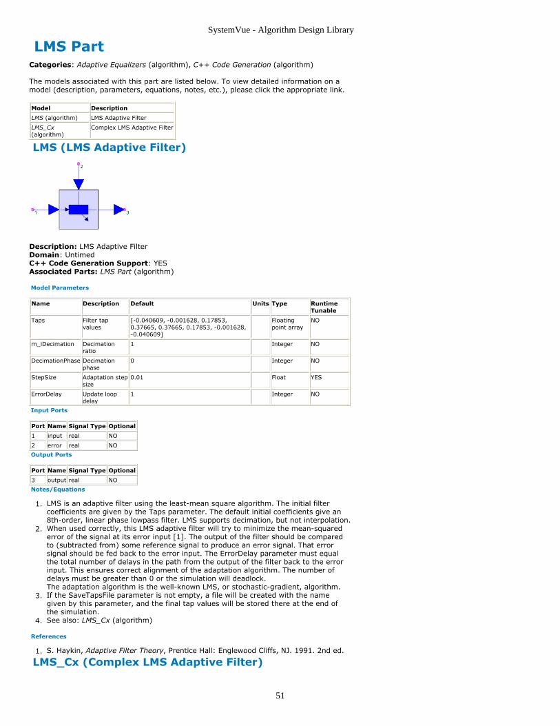
SystemVue - Algorithm Design Library
51
LMS PartCategories: Adaptive Equalizers (algorithm), C++ Code Generation (algorithm)
The models associated with this part are listed below. To view detailed information on amodel (description, parameters, equations, notes, etc.), please click the appropriate link.
Model Description
LMS (algorithm) LMS Adaptive Filter
LMS_Cx(algorithm)
Complex LMS Adaptive Filter
LMS (LMS Adaptive Filter)
Description: LMS Adaptive FilterDomain: UntimedC++ Code Generation Support: YESAssociated Parts: LMS Part (algorithm)
Model Parameters
Name Description Default Units Type RuntimeTunable
Taps Filter tapvalues
[-0.040609, -0.001628, 0.17853,0.37665, 0.37665, 0.17853, -0.001628,-0.040609]
Floatingpoint array
NO
m_iDecimation Decimationratio
1 Integer NO
DecimationPhase Decimationphase
0 Integer NO
StepSize Adaptation stepsize
0.01 Float YES
ErrorDelay Update loopdelay
1 Integer NO
Input Ports
Port Name Signal Type Optional
1 input real NO
2 error real NO
Output Ports
Port Name Signal Type Optional
3 output real NO
Notes/Equations
LMS is an adaptive filter using the least-mean square algorithm. The initial filter1.coefficients are given by the Taps parameter. The default initial coefficients give an8th-order, linear phase lowpass filter. LMS supports decimation, but not interpolation.When used correctly, this LMS adaptive filter will try to minimize the mean-squared2.error of the signal at its error input [1]. The output of the filter should be comparedto (subtracted from) some reference signal to produce an error signal. That errorsignal should be fed back to the error input. The ErrorDelay parameter must equalthe total number of delays in the path from the output of the filter back to the errorinput. This ensures correct alignment of the adaptation algorithm. The number ofdelays must be greater than 0 or the simulation will deadlock.The adaptation algorithm is the well-known LMS, or stochastic-gradient, algorithm.If the SaveTapsFile parameter is not empty, a file will be created with the name3.given by this parameter, and the final tap values will be stored there at the end ofthe simulation.See also: LMS_Cx (algorithm)4.
References
S. Haykin, Adaptive Filter Theory, Prentice Hall: Englewood Cliffs, NJ. 1991. 2nd ed.1.
LMS_Cx (Complex LMS Adaptive Filter)

SystemVue - Algorithm Design Library
52
Description: Complex LMS Adaptive FilterDomain: UntimedC++ Code Generation Support: YESAssociated Parts: LMS Part (algorithm)
Model Parameters
Name Description Default Units Type RuntimeTunable
Taps Filter tap values [-0.040609, -0.001628, 0.17853,0.37665, 0.37665, 0.17853, -0.001628, -0.040609]
Complexarray
NO
Decimation Decimation ratio 1 Integer NO
DecimationPhase Decimation phase 0 Integer NO
StepSize Adaptation step size 0.01 Float YES
ErrorDelay Update loop delay 1 Integer NO
SaveTapsFile Filename in which tosave final tap values
Text NO
Input Ports
Port Name Signal Type Optional
1 input complex NO
2 error complex NO
Output Ports
Port Name Signal Type Optional
3 output complex NO
Notes/Equations
LMS_Cx is a complex adaptive filter using the least-mean square algorithm. For more1.details see LMS (algorithm).

SystemVue - Algorithm Design Library
53
NonLinearityCx PartCategories: Adaptive Equalizers (algorithm)
The models associated with this part are listed below. To view detailed information on amodel (description, parameters, equations, notes, etc.), please click the appropriate link.
Model Description
NonLinearityCx(algorithm)
Non-linear function for use in blind adaptive algorithms.

SystemVue - Algorithm Design Library
54
NonLinearityCx
Description: Non-linear function for use in blind adaptive algorithms.Domain: UntimedC++ Code Generation Support: NOAssociated Parts: NonLinearityCx Part (algorithm)
Model Parameters
Name Description Default Units Type RuntimeTunable
Range
BlindAlgorithm Choice of blind adaptive algorithm to use.:Decision Directed (Luckly) , ConstantModulus Algorithm (Godard) , Sato ,Benveniste-Goursat , Stop-and-Go (Picchiand Prati)
DecisionDirected(Luckly)
Enumeration NO (0:4)
ModType Modulation type: BPSK , QPSK , PSK8 ,PSK16 , QAM16 , QAM32 , QAM64 ,QAM128 , 256QAM , User_Defined
BPSK Enumeration NO (0:9)
MappingTable Constellation table (used whenModType=User_Defined)
[1+j*0,-1+j*0]
Complexarray
NO [-∞:∞]
Input Ports
Port Name Signal Type Optional
1 inputSignal complex NO
Output Ports
Port Name Signal Type Optional
2 outputSignal complex NO
Notes/Equations
This model implements a set of non-linear functions for use in blind adaptive1.algorithms. A range of blind adaptive algorithms can be constructed by using thispart in conjunction with the adaptive filter cores.The DDM and Godard algorithms work with complex-valued or real-valued2.modulation formats. Sato, Benveniste-Goursat and Stop-and-Go algorithms onlywork with real-valued modulation formats.

SystemVue - Algorithm Design Library
55
AddEnv PartCategories: Analog/RF (algorithm)
The models associated with this part are listed below. To view detailed information on amodel (description, parameters, equations, notes, etc.), please click the appropriate link.
Model Description
AddEnv(algorithm)
Envelope SignalAdder
AddEnv (Complex Envelope Signal Adder)
Description: Envelope Signal AdderDomain: TimedC++ Code Generation Support: NOAssociated Parts: AddEnv Part (algorithm)
Model Parameters
Name Description Default Units Type RuntimeTunable
Range Symbol
OutputFc Output characterization frequencyfor the combined signal: Min, Max,Center, User defined
Center Enumeration NO O
UserDefinedFc User defined outputcharacterization frequency
100e6 Hz Float NO [0:∞)† F
Input Ports
Port Name Description Signal Type Optional
1 input input signals multipleenvelope
NO
Output Ports
Port Name Description Signal Type Optional
2 output output signal envelope NO
Notes/Equations
The AddEnv model outputs the sum of the complex envelope inputs.1.This model reads 1 sample from all inputs and writes 1 sample to the output.2.Each input may have either a real baseband value or a complex value defined at a3.specific characterization frequency. The output characterization frequency NewFc is determined by the configuration of4.inputs and the parameters, OutputFc and UserDefinedFc.
If any input is a real baseband signal, then the output will be a real basebandsignal.Otherwise, the output will be a complex envelope signal defined at acharacterization frequency NewFc as follows.
If OutputFc is Min, NewFc is set to the minimum input characterizationfrequencies.If OutputFc is Max, NewFc is set to the maximum input characterizationfrequencies.If OutputFc is Center, NewFc is set to the average of the maximum andminimum input characterization frequencies.If OutputFc is User defined, NewFc is set to the UserDefinedFc parameter.
Note that if UserDefinedFc is positive, then all inputs require a nonzero characterizationfrequency.
All inputs are converted to their equivalent representation at NewFc before summing.5.A complex envelope value OldIQ at characterization frequency OldFc is converted to a6.NewIQ at characterization frequency NewFc at time t as follows.
NewIQ is set to If NewFc is zero, the imaginary part of NewIQ is set to zero.
A warning message is displayed once if an input sample rate is too small to make the7.transformation without loss of information.
See:SubEnv (algorithm)MpyEnv (algorithm)MpyMultiEnv (algorithm)

SystemVue - Algorithm Design Library
56
AddNDensity PartCategories: Analog/RF (algorithm), Communications (algorithm)
The models associated with this part are listed below. To view detailed information on amodel (description, parameters, equations, notes, etc.), please click the appropriate link.
Model Description
AddNDensity(algorithm)
Add Noise Density to Input
AddNDensity (Add Noise Density)
Description: Add Noise Density to InputDomain: TimedC++ Code Generation Support: NOAssociated Parts: AddNDensity Part (algorithm)
Model Parameters
Name Description Default Units Type RuntimeTunable
Range
NDensityType Noise density type: Constantnoise density, Noise density vsfreq
Constantnoise density
Enumeration NO
NDensity Noise power spectral density 0.0 W Float NO [0:∞)
NDensityFreq Noise spectral densityspecification frequency values(Hz)
Floating pointarray
NO
NDensityPower Noise spectral densityspecification power density values(dBm/Hz)
Floating pointarray
NO
RefR Reference resistance 50 ohm Float NO (0:∞)
Input Ports
Port Name Description Signal Type Optional
1 input input signal envelope NO
Output Ports
Port Name Description Signal Type Optional
2 output output signal envelope NO
Notes/Equations
This model adds noise to the input signal.1.At every execution, it reads 1 sample from the input and writes 1 sample to the2.output.If NDensityType is set to Constant noise density, then the noise added is white3.Gaussian.The noise density is specified in the NDensity parameter. Although the units for thisparameter are power units the value is interpreted as power spectral density, that is,power per frequency unit (Hz).The total noise power added to the input signal is NDensity × BW, where
NDensity is the noise power spectral density in Watts/HzBW is the simulation bandwidth (equal to SR for a complex envelope signal andSR / 2 for a real baseband signal; SR is the input signal sample rate) in Hz.The rms noise voltage level is .The value of NDensity (in Watts/Hz) is related to temperature (in °Kelvin) as k·T, where k is the Boltzmann constant (1.3806504e-23). At the standard systemtemperature of 290° Kelvin (16.85° Celsius), the NDensity is 4.00388587e-21Watts/Hz (-173.975 dBm/Hz).
If NDensityType is set to Noise density vs freq, then the spectral profile of the noise4.added can be specified using the NDensityFreq (values need to be in Hz) andNDensityPower (values need to be in dBm/Hz) array parameters.

SystemVue - Algorithm Design Library
57
AmplifierBB PartCategories: Analog/RF (algorithm)
The models associated with this part are listed below. To view detailed information on amodel (description, parameters, equations, notes, etc.), please click the appropriate link.
Model Description
AmplifierBB(algorithm)
Baseband Polynomial Amplifier with NoiseFigure
AmplifierBB (Baseband Nonlinearity With NoiseFigure)
Description: Baseband Polynomial Amplifier with Noise FigureDomain: TimedC++ Code Generation Support: NOAssociated Parts: AmplifierBB Part (algorithm)
Model Parameters
Name Description Default Units Type RuntimeTunable
Range
Offset DC offset voltage 0 Float NO (-∞:∞)
GainUnit Gain unit for the Gain parameter orthe optional voltage controlled gaininput: voltage, dB
voltage Enumeration NO
Gain Gain with units defined by GainUnit(used if optional voltage controlledgain input not used)
1 Float NO (-∞:∞)
NoiseFigure Input noise figure in dB 0 Float NO [0:∞)
SOIout Output second order intercept powerin dBm
40 Float NO (-∞:∞)
TOIout Output third order intercept power indBm
30 Float NO (-∞:∞)
HigherOrderTerms Higher order intercept terms 4th to11th in dBm
[ ] Floating pointarray
NO (-∞:∞)
RefR Reference resistance 50 ohm Float NO (0:∞)
Input Ports
Port Name Description Signal Type Optional
1 input input signal real NO
2 control gain control real YES
Output Ports
Port Name Description Signal Type Optional
3 output output signal real NO
Notes/Equations
AmplifierBB models a baseband nonlinearity including noise figure.1.This block reads 1 sample from input and writes 1 sample to output.2.The small signal gain value is based on either the Gain parameter value or on the3.optional control value. The control input is optional and when used the value at thatpin is used instead of the Gain parameter value. In the following discussion, the Gainvalue generally refers to the control input value as well.The nonlinearity is defined by the parameters Gain, SOIout, TOIout and RefR and by4.curve fitting the nonlinear parameters with a second, third, or higher orderpolynomial. The higher order polynomial is used if the HigherOrderTerms arespecified. SOI, TOI and HigherOrderTerms are ignored if set to 200 dBm or higher.Nonlinear model with SOI is defined as follows.5.
Let y = c 1 x - c 2 x 2
wherex = input voltagey = output voltagec 1 = small signal gain = Gain

SystemVue - Algorithm Design Library
58
c 2 = second order gain factor
Saturation occurs at the peak x = x_max. This occurs when dy/dx = 0c 1 - 2 c 2 x_max = 0. Therefore, x_max = (c 1 / 2) / c 2.
y_max = c 1 x_max - c 2 x_max 2
Given the output, SOI is specified in dBm into RefR ohms, then c 2 is derived as
follows.
Let SOIv be SOI in terms of output peak volts.SOI occurs at x i such that c 1 x i = c 2 x i
2 = SOIv. Therefore, c 2 = c 12 /
SOIv.This value for c 2 implies that a positive signal experiences expansion, but a
negative signal will have compression.Nonlinear model with TOI6.
Let y = c 1 x + c 3 x 3
wherex = input voltagey = output voltagec 1 = Gain
c 3 = third order gain factor
Saturation occurs at the peak x = x_max. This occurs when dy/dx = 0c 1 + 3 c 3 x_max 2 = 0
y_max = c 1 x_max + c 3 x_max 3
Given the output, TOI is specified in dBm into RefR ohms, then c 3 is derived as
follows.
Let TOIv be TOI in terms of output peak volts.TOI is defined for a two tone input signal, x(t).The expansion for y(t) = c 1 x(t) + c 3 x 3(t) results in fundamental terms
at w1, w2 and third order terms at 2 w1 - w2, 2 * w2 - w1.See note One and Two Tone Response for SOI and TOI.After the trigonometric expansion,
the first order term is c 1
the third order term is: (3/4) c 3 x 3
TOI occurs at x i such at c 1 x i = -(3/4) c 3 x 3 = TOIv
Thus c 3 = -(4/3) c 13 / TOIv 2
Nonlinear model with SOI and TOI7.Let y = c 1 x + c 2 x 2 + c 3 x 3
wherex = input voltagey = output voltagec 1 = Gain
c 2 = second order gain factor
c 3 = third order gain factor
c 2 and c 3 are derived as described in the notes above.
Saturation occurs at the peak x = x_max. This occurs when dy/dx = 0c 1 - 2 c 2 x_max + 3 c 3 x_max 2 = 0
Using the quadratic equations solution that makes x_max positive
This value of x_max is always positive.y_max = c 1 x_max - c 2 x_max 2 + c 3 x_max 3
This y_max value is the limit for a positive x_max signal.For a negative signal, there will be another limiting value that is calculated usingthe above expression for the other quadratic equation solution.
When HigherOrderTerms are defined (with values less than 200 dBm), then a similar8.process to that described above is used to derive the nonlinearity polynomialcoefficiants along with the positive and negative saturation characteristics.The noise is defined by the parameters NoiseFigure and RefR.9.
Letk = Boltzmann constant = 1.3806504e-23 Joules/Kelvinsr = simulation sample rate at this block inputt0 = reference temperature at 290 Kelvinnf = 10 (NoiseFigure/10)
Then, the rms noise voltage, vn_rms is calculated as follows.

SystemVue - Algorithm Design Library
59
vn_rms is used to generate a Gaussian random variate that is added to theinput signal before the signal is amplified through the nonlinearity.
One and Two-Tone Response for SOI and TOI
Let y = c 1 x + c 2 x 2 + c 3 x 3
wherey = output voltagec 1 = small signal gain
c 2 = second order gain factor
c 3 = third order gain factor
For one-tone excitation, , the response is:
For two-tone excitation, , the response is:

SystemVue - Algorithm Design Library
60
Amplifier PartCategories: Analog/RF (algorithm)
The models associated with this part are listed below. To view detailed information on amodel (description, parameters, equations, notes, etc.), please click the appropriate link.
Model Description
Amplifier(algorithm)
Nonlinear Amplifier with Noise Figure
Amplifier (Nonlinear Gain)
Description: Nonlinear Amplifier with Noise FigureDomain: TimedC++ Code Generation Support: NOAssociated Parts: Gain Part (algorithm), Amplifier Part (algorithm)
Model Parameters
Name Description Default Units Type RuntimeTunable
Range
GainUnit Gain unit for the Gain parameter or the optionalvoltage controlled gain input: voltage, dB
voltage Enumeration NO
Gain Gain with units defined by GainUnit (used ifoptional voltage controlled gain input not used)
1 Float NO (-∞:∞)
NoiseFigure Input noise figure in dB 0 Float NO [0:∞)
GCType Gain compression type: none, TOI, dBc1,TOI+dBc1, PSat+GCSat+TOI,PSat+GCSat+dBc1, PSat+GCSat+TOI+dBc1,RappNonlinearity, Gain compression vs inputpower, AM/AM and AM/PM vs input power
none Enumeration NO
TOIout Output third order intercept power 0.1 W Float NO (0:∞)†
dBc1out Output 1 dB gain compression power 0.01 W Float NO (0:∞)†
PSat Saturation power 0.032 W Float NO (0:∞)†
GCSat Gain compression at saturation in dB 3 Float NO [3:7]†
RappS Rapp nonlinearity smoothness factor 3 Integer NO (0:∞)
GComp Array of triple values for Input Power(dBm) andeither Gain(dB)/Phase(deg) change from smallsignal or AM-to-AM(dB/dB)/AM-to-PM(deg/dB)
[0, 0,0]
Floatingpoint array
NO ‡
RefR Reference resistance 50 ohm Float NO (0:∞)
Input Ports
Port Name Description Signal Type Optional
1 input input signal envelope NO
2 control gain control real YES
Output Ports
Port Name Description Signal Type Optional
3 output output signal envelope NO
Notes/Equations
Amplifier models a nonlinearity including noise figure for use with either baseband or1.complex envelope signals.This block reads 1 sample from input in and writes 1 sample to output out.2.The small signal gain value is based on either the Gain parameter value or on the3.optional control input value if used. The control input does not need to be connected.It is optional and when used the value at that pin is used instead of the Gainparameter value. In the following discussion, the Gain value implies the control inputvalue as well.The nonlinearity is defined by the parameters GCType, TOIout, dBc1out, PSat, GCSat,4.RappS, GComp and RefR. All nonlinear models except those based on GComp areachieved by curve fitting nonlinear parameters with an odd order nonlinearpolynomial. The GComp based nonlinearities are table based with interpolationbetween points.The general nonlinearity has this output power versus input power characteristic.5.

SystemVue - Algorithm Design Library
61
Nonlinear model with TOI6.Let y = c 1 x + c 3 x 3
wherex = input voltagey = output voltagec1 = small signal gain ( Gain )c3 = third order gain factor
See detail discussion in the documentation for the AmplifierBB block. SeeAmplifierBB (algorithm).
Nonlinear model with dBc17.Let y = c 1 x + c 3 x 3
wherex = input voltagey = output voltagec1 = small signal gain ( Gain )c3 = third order gain factor
Given the output dBc1out in dBm into RefR ohms, then c 3 is derived as follows.
dBc1v = dBc1out in terms of output peak volts
dBc1out occurs when y is 1 dB compressed.This occurs when y 1 = c 1 x 1 + c 3 x 1
3 = 0.891 c 1 x 1where
-1 dB = 20 log 10 (0.891)
y 1 = dBc1v
x 1 = (dBc1v / 0.891) / c 1
c 3 = (y 1 – c 1 x 1) / x 13
Saturation occurs as for the TOI nonlinearity:
y_max = c 1 x_max + c 3 x_max 3
Nonlinear model with TOI and dBc18.Let y = c 1 x + c 3 x 3 + c 5 x 5
wherex = input voltagey = output voltagec 1 = small signal gain
c 3 = third order gain factor
c 5 = fifth order gain factor
c 3 is same as that derived for the TOI nonlinearity.
Given the output dBc1out in dBm into RefR ohms, then c 5 is derived as follows:
dBc1v = dBc1 in terms of output peak volts
dBc1 occurs when y is 1 dB compressed.This occurs when y 1 = c 1 x 1 + c 3 x 1
3 + c 5 x 5 = 0.891 c 1 x 1where
-1 dB = 20 log 10 (0.891)
y 1 = dBc1v
x 1 = (dBc1v / 0.891) / c 1
c 5 = (y 1 – c 1 x 1 – c 3 x 13) / x 1
5
The minimum TOI occurs when c 5 = 0

SystemVue - Algorithm Design Library
62
Therefore, the minimum TOI is defined whenc 3 = -(1 - 0.891)(0.891 2)(c 1
3) / dBc1v 2
Saturation occurs at the peak x = x_max. This occurs when dy/dx = 0c 1 + 3 c 3 x_max 2 + 5 c 5 x_max 4 = 0
Using the minimum quadratic equations solution
y_max = c 1 x_max + c 3 x_max 3 + c 5 x_max 5
Nonlinear model with PSat, GCSat, TOI and dBc19.Let y = c 1 x + c 3 x 3 + c 5 x 5 + c 7 x 7 + c 9 x 9 + c 11 x 11
wherex = input voltagey = output voltagec 1 = small signal gain
c 3, c 5, c 7, c 9, c 11 = 3rd, 5th, 7th, 9th, 11th order gain factor; c 3 < 0, c 5< 0
For GCType = PSat+GCSat+TOI, dBc1out = TOIout - dB_offsetFor GCType = PSat+GCSat+dBc1, TOIout = dBc1out + dB_offsetFor complex envelope signals, dB_offset = 10.6357 dB, otherwise for basebandsignals, dB_offset = 11.8851 dB.The c 11 factor is used to improve the stability of the polynomial expression;
otherwise the polynomial is more likely to have gain expansion or reduced rangeof usage.c 3 is based on TOIout only and is as derived for the TOI nonlinearity.
GCSatR = voltage compression ratio = 10 (GSat / 20)
y s = output peak voltage at saturation =
x s = input peak voltage at saturation = PSatv × GCSatR / c 1
y 1 = output peak voltage at 1dB compression =
x 1 = input peak voltage at 1dB compression = (dBc1v / 0.891) / c 1To derive c 5, c 7, c 9 and c 11. Setup 4 equations with 4 unknowns.
At 1dB compression:c 1 x 1 + c 3 x 1
3 + c 5 x 15 + c 7 x 1
7 + c 9 x 19 + c 11 x 1
11 = y 1At saturation there is GCSat dB compressionc 1 x s + c 3 x s
3 + c 5 x s5 + c 7 x s
7 + c 9 x s9 + c 11 x s
11 = y sAt saturation set dy/dx = 0c 1 + 3 c 3 x 1
2 + 5 c 5 x 14 + 7 c 7 x 1
6 + 9 c 9 x 18 + 11 c 11 x 1
10 = 0
At saturation set the second derivative of y with respect to x to zero2 × 3 c 3 x 1 + 4 × 5 c 5 x 1
3 + 6 × 7 c 7 x 15 + 8 × 9 c 9 x 1
7 + 10 × 11 c 11
x 19 = 0
The four equations are solved for the four unknowns: c 5, c 7, c 9, c 11
The following parameter value limits are defined.For GCType = PSat+GCSat+TOI+dBc1dBc1out_dBm + 0.5 × GCSat_dB – 1 < PSat_dBm < dBc1out_dBm + 13 -GCSat_dBFor GCType = PSat+GCSat+TOI+dBc1TOIout_dBm_LoLimit =dBc1out_dBm + dB_offset – 1 – 0.5 × ( (dBc1out_dBm + 13 – GCSat_dB)– PSat_dBm )TOIout_dBm_HiLimit =dBc1out_dBm + dB_offset + ( (dBc1out_dBm + 13 – GCSat_dB) –Psat_dBm ) 2
Nonlinear model with Rapp Nonlinearity10.Let y = c 1 abs (x) / ( 1 + (c1*abs (x) /xs)(2*s) )(1/(2*s))
wherec 1 = Gain
s > 0; s = nonlinearity smoothness factor = RappSx s >= 0; x s = input peak voltage at saturation
GCSatR = voltage compression ratio = 10 (GSat / 20)
y s = output peak voltage at saturation =
x s = input peak voltage at saturation = PSatv × GCSatR / c 1This nonlinear model was developed for solid state power amplifiers, produces asmooth transition for the AM/AM conversion as the input amplitude approaches

SystemVue - Algorithm Design Library
63
saturation, and has no AM/PM conversion.The reference for the Rapp nonlinear model is:Rapp C., "Effects of HPA-nonlinearity on a 4-DPSK/OFDM-signal for a digitalsound broadcasting system," in Proc. of the Second European Conf. on SatelliteComm.,Liège, Belgium, Oct. 1991.
Nonlinear model with Gain compression versus input power11.This nonlinear model is defined by the small signal gain, Gain, and the array of triplevalues for input power(dBm), gain change (dB) and phase change (deg) from smallsignal.
Define:dB(G ss) = small signal gain in dB
phase(G ss) = small signal phase in deg
P = input power in dBmO = output power in dBmOPh = output phase in degGC = gain change from small signal in dBGC[i] = O[i] – P[i] – dB(G ss);
GC[i] = (O[i] – O[i-1]) – (P[i] – P[i-1]) + GC[i-1]PC = phase change from small signal in degPC[i] = OPh[i] – phase(G ss);
PC[i] = (OPh[i] – OPh[i-1]) + PC[i-1];Gain and phase change between the consecutive points is found using linearinterpolation.
Nonlinear model with AM/AM and AM/PM versus input power12.This nonlinear model is defined by the small signal gain, Gain, and the array of triplevalues for input power(dBm), AM-to-AM (dB/dB), and AM-to-PM (deg/dB).The model is achieved by relating to the nonlinear model with Gain compressionversus input power. See the prior note for the definition of P, O, OPh, GC and PC
DefineAM_to_AM = AM = (delta output power in dB)/(delta input power in dB)AM_to_PM = PM = (delta output phase in deg)/(delta input power in dB)
By definitionAM[i] = 0.5 * ( dO[i]/dP[i] + dO[i+1]/dP[i+1] )PM[i] = 0.5 * ( dOPh[i]/dP[i] + dOPh[i+1]/dP[i+1] )Where
dO[i] = O[i] – O[i-1] with dO[0] = 0;dOPh[i] = OPh[i] – OPh[i-1] with dOPh[0] = 0;dP[i] = P[i] – P[i-1] with dP[0] = dP[1];
Given the set of values for AM[i] and PM[i], the associated value for GC[i] andPC[i] are derived. Then the nonlinearity is as defined in the previous note.
The noise is defined by the parameters NoiseFigure and RefR.13.Let
k = Boltzmann constant = 1.3806504e-23 Joules/Kelvinsr = simulation sample rate at this block inputfactor = 2 for real baseband signal, = 1 for complex envelope signalst0 = reference temperature = 290 Kelvinnf = 10 (NoiseFigure/10)
vn_rms = rms noise voltageThen
vn_rms is used to generate a Gaussian random variate that is added to theinput signal before the signal is amplified through the nonlinearity.

SystemVue - Algorithm Design Library
64
AtoD_ADI PartCategories: Analog/RF (algorithm)
The models associated with this part are listed below. To view detailed information on amodel (description, parameters, equations, notes, etc.), please click the appropriate link.
Model Description
AtoD_ADI(algorithm)
Analog to Digital Converter for ADI ADCModels

SystemVue - Algorithm Design Library
65
AtoD_ADI
Description: Analog to Digital Converter for ADI ADC ModelsDomain: TimedC++ Code Generation Support: NOAssociated Parts: AtoD ADI Part (algorithm)
Model Parameters

SystemVue - Algorithm Design Library
66
Name Description Default Units Type RuntimeTunable
Model ADC type A-to-D model: User specifiedmodel, AD6645_80.adc,AD6645_105.adc, AD9214_65_2V.adc,AD9214_80_1V.adc,AD9214_105_1V.adc, AD9215_65.adc,AD9215_80.adc, AD9215_105.adc,AD9216_65.adc, AD9216_80.adc,AD9216_105.adc, AD9218_40_1V.adc,AD9218_65_2V.adc,AD9218_80_1V.adc,AD9218_105_1V.adc, AD9219_40.adc,AD9219_65.adc, AD9222_40.adc,AD9222_50.adc, AD9226_2V.adc,AD9228_40.adc, AD9228_65.adc,AD9229_50.adc, AD9229_65.adc,AD9230_170.adc, AD9230_210.adc,AD9230_250.adc, AD9233_105.adc,AD9233_125.adc, AD9236.adc,AD9237_20.adc, AD9237_40.adc,AD9237_65.adc, AD9238_20.adc,AD9238_40.adc, AD9238_65.adc,AD9244_40.adc, AD9244_65.adc,AD9245_20.adc, AD9245_40.adc,AD9245_65.adc, AD9245_80.adc,AD9246_105.adc, AD9246_125.adc,AD9248_20.adc, AD9248_40.adc,AD9248_65.adc, AD9252.adc,AD9254.adc, AD9259.adc, AD9287.adc,AD9289.adc, AD9430_170_LVDS.adc,AD9430_210_LVDS.adc,AD9433_105.adc, AD9433_125.adc,AD9444.adc, AD9445_105_2V.adc,AD9445_105_3p2V.adc,AD9445_125_2V.adc,AD9445_125_3p2V.adc,AD9446_80_2V.adc,AD9446_80_3p2V.adc,AD9446_100_2V.adc,AD9446_100_3p2V.adc,AD9460_80_3p4V.adc,AD9460_105_3p4V.adc,AD9461_125_3p4V.adc,AD9461_130_3p4V.adc, AD9480.adc,AD9600.adc, AD9601.adc,AD9626_170.adc, AD9626_210.adc,AD9626_250.adc, AD9627-11.adc,AD9627.adc, AD9640.adc, AD80141.adc,Ideal_8_Bit.adc, Ideal_10_Bit.adc,Ideal_12_Bit.adc, Ideal_14_Bit.adc
Userspecifiedmodel
Enumeration NO
ModelDirType Model directory type: Default, Userdefined
Default Enumeration NO
ModelDir User defined directory for model adc files Text NO
UserModel User specified A-to-D model Filename NO
UserNBits User specified number of bits in the A-to-D model
8 Integer NO
UserMinSR User specified minimum sample rate(encode rate)
0 Hz Float NO
UserMaxSR User specified maximum sample rate(encode rate)
1e12 Hz Float NO
UserCommonModeOffset User specified common mode offsetvoltage applied to input signal
0 V Float NO
UserInputSpan User specified input signal span 2 V Float NO
UserDigitalFormat User specified output digital format:Offset binary, Twos-complement
Twos-complement
Enumeration NO
CenterFreq Spectral center frequency of analoginput
0 Hz Float NO
NyquistZone Value representing the analog inputNyquist zone; use n when n*SR/2 < f <(n+1)*SR/2
1 Integer NO
EnableExtJitter Enable external jitter: NO, YES NO Enumeration NO
ExtJitter External RMS jitter applied to the inputsignal
0 s Float NO
Input Ports
Port Name Description Signal Type Optional
1 A_in input analogsignal
envelope NO
Output Ports

SystemVue - Algorithm Design Library
67
Port Name Description Signal Type Optional
2 A_out output sampled analog signal envelope NO
3 D_I output NBit word as integer for I channel int NO
4 D_Q output NBit word as integer for Q channel int NO
Notes/Equations
This component models analog-to-digital converters from Analog Devices with1.reference to Analog Devices part numbers. The input at A_in can be a real basebandsignal or a complex envelope signal. The output digital words are in integer form.When the input is a real baseband signal, the output digital word is at the D_Ioutput. When the input is a complex envelope signal, the D_I output contains thedigital word for the I envelope and the D_Q ouput contains the digital word for the Qenvelope. The A_out contains the quantized form of the input signal. If A_in is acomplex envelope signal, then the A_out is also a complex envelope signal at thesame characterization frequency.This block reads 1 sample from the input and writes 1 sample to the outputs.2.ModelDir is the computer disk directory location in which the Analog Devices AtoD3.model files (*.adc) are located. The default location is in the SystemVue installationdirectory (typically C:\Program Files\SystemVue(Version)) under Model\ADI. Theuser can use these model files delivered with SystemVue or use other Analog DevicesAtoD model files obtained from Analog Devices and located in another directory.When Model is not 'User specified model'4.The Model value is the name of an Analog Devices AtoD model file that is deliveredwith SystemVue. By selecting one of these predefined model, the full characteristicsare defined and used. For these models, the simulator prints out the values for NBits,MinSR, MaxSR, CommonModeOffset, InputSpan and DigitalFormat associated withthe selected Analog Devices AtoD model.When Model is 'User specified model'5.The UserModel is the Analog Devices *.adc filename that the user separatelyobtained and would like to use. This option is available when the predefined *.adcfilenames are not what the user wants to use and would like to use instead otherAnalog Devices AtoD models. The UserNBits, UserMinSR, UserMaxSR,UserCommonModeOffset, UserInputSpan, and UserDigitalFormat values are to beentered by the user as is defined for the UserModel listed by the user and are valueto be obtained from Analog Devices for the model listed.Every simulation sample results in sampling the input A_in and quantization of that6.input resulting in the output values. When EnableExtJitter = YES, then the ExtJitterdefines the RMS jitter applied to the input A_in before sampling.The Analog Devices AtoD (*.adc) model is defined for use with the input signals in7.the range [ CommonModeOffset, CommonModeOffset + InputSpan ]. TheCommonModeOffset bias is automatically applied internally to the AtoD_ADI inputA_in. Thus, the AtoD_ADI input A_in is defined for use with A_in in the range [ -InputSpan / 2, InputSpan / 2 ), and limited to these limits when A_in is outside thisrange. The CommonModeOffset and InputSpan are automatically defined when Modelis not 'User specified model'. They are defined by UserCommonModeOffset andUserInputSpan when Model is 'User specified model'.Quantization of the input A_in8.NBits, InputSpan and DigitalFormat are used to quantize the input A_in to generatethe digital words that appear at the integer outputs D_I and D_Q and the quantizedanalog output A_out. These values are either predefined when Model is not 'Userspecified model', or are user specified when Model is 'User specified model'. DefineVRef = InputSpan/2. Define LSB = least significant bit = 2 × VRef / 2 NBits .The conversion thresholds for A_in are {-VRef + i × LSB}, where i = 1, ... , 2 NBits -1.When DigitalFormat is 'Offset binary', the digital words span integer values in therange [ 0, 2^ NBits - 1 ].When DigitalFormat is 'Twos-complement', the digital words span integer values inthe range [ -2^( NBits /2), 2^( NBits /2) - 1 ].A_out output is in the range of [-(VRef - 0.5 LSB), (VRef - 0.5 LSB)] with values {-VRef + (i - 0.5) × LSB}, where i = 1, ... , 2 NBits .The Analog Devices AtoD models all have a start up transient time (Latency) during9.which time the output values are random values.The Analog Devices AtoD models allow the user to specify the spectral center10.frequency of the analog signal (CenterFreq, when A_in is real) and the analog inputNyquist zone to improve AtoD model behavior.See the Analog Devices AtoD documentation for more detail on their AtoD models.11.http://www.analog.com/en/analog-to-digital-converters/ad-converters/products/index.html

SystemVue - Algorithm Design Library
68
AtoD_ADI_PMF PartCategories: Analog/RF (algorithm), C++ Code Generation (algorithm)
The models associated with this part are listed below. To view detailed information on amodel (description, parameters, equations, notes, etc.), please click the appropriate link.
Model Description
AtoD_ADI_PMF(algorithm)
Analog to Digital Converter for ADI PMF Models

SystemVue - Algorithm Design Library
69
AtoD ADI PMF
Description: Analog to Digital Converter for ADI PMF ModelsDomain: TimedC++ Code Generation Support: YESAssociated Parts: AtoD ADI PMF Part (algorithm)
Model Parameters
Name Description Default Units Type RuntimeTunable
PMFModel PMF type A-to-D model: AD6655.pmf,AD6657.pmf, AD9262.pmf,AD9271.pmf, AD9272.pmf,AD9273.pmf
AD6655.pmf Enumeration NO
ModelDirType Model directory type: Default, Userdefined
Default Enumeration NO
ModelDir User defined directory for model adcand pmf files
Text NO
DisplayPMF_Info Display PMF model information: No,Setup information, Setup informationand all available states
No Enumeration NO
Set6655_Mode PMF model 6655 mode: HB Only, HB +FIR, NCO + HB, NCO + HB + FIR, NCO+ HB + FIR + fadc/8
HB Only Enumeration NO
Set6657_Mode PMF model 6657 mode: ADC Only, ADC+ NS (22%), ADC + NS (33%)
ADC Only Enumeration NO
Set9262_Mode PMF model 9262 mode: 10 MHzBandwidth, 5 MHz Bandwidth, 2.5 MHzBandwidth
10 MHzBandwidth
Enumeration NO
LowPass Enable halfband low pass mode: NO,YES
YES Enumeration NO
ReverseSpec Enable spectrum reversal mode: NO,YES
NO Enumeration NO
DoubleFIRScale Double FIR scale factor: NO, YES NO Enumeration NO
DecimationPhase Decimation phase 0 Integer NO
NCO_Freq NCO frequency 0 Hz Float NO
NCO_PhaseOffset NCO phase offset in degrees 0 Float NO
NoiseShapeTuningWord Noise shape tuning word 0 Integer NO
NCO_Kout_m NCO Kout parameter m 16 Float NO
LNA_Gain1 LNA scalar gain: Gain1 14, Gain1 15.6,Gain1 18
Gain1 14 Enumeration NO
LNA_Gain2 LNA scalar gain: Gain2 15.6, Gain217.9, Gain2 21.3
Gain2 15.6 Enumeration NO
VGA_Gain VGA scalar gain 0 Float NO
PGA_Gain PGA scalar gain 0 Float NO
PGA_Atten PGA scalar attenuation: Atten 21,Atten 24, Atten 27, Atten 30
Atten 24 Enumeration NO
LowerCutOffFreq Lower cutoff frequency: LPF 0, LPF300000, LPF 700000
LPF 0 Enumeration NO
AAF_k AAF k parameter: AAF k 0.7, AAF k0.8, AAF k 0.9, AAF k 1.0, AAF k 1.1,AAF k 1.2, AAF k 1.3
AAF k 0.7 Enumeration NO
HPF_CutOffFreq HPF Cutoff Frequency (not working; tobe fixed): HPF Flp/20.7, HPF Flp/11.5,HPF Flp/7.9, HPF Flp/6.0, HPF Flp/4.9,HPF Flp/4.1, HPF Flp/3.5, HPF Flp/3.1,HPF DC
HPF Flp/20.7 Enumeration NO
LPF_fc_vs_fs LPF fc percentage of fs: LPF 1/3, LPF1/4.5
LPF 1/3 Enumeration NO
CenterFreq Spectral center frequency of analoginput
0 Hz Float NO
NyquistZone Value representing the analog inputNyquist zone; use n when n*SR/2 < f< (n+1)*SR/2
0 Integer NO
EnableExtJitter Enable external jitter: NO, YES NO Enumeration NO
ExtJitter External RMS jitter applied to the inputsignal
0 s Float NO
Input Ports

SystemVue - Algorithm Design Library
70
Port Name Description Signal Type Optional
1 A_in input analogsignal
envelope NO
Output Ports
Port Name Description Signal Type Optional
2 I_out output sampled analog I signal envelope NO
3 Q_out output sampled analog Q signal envelope NO
4 D_I output NBit word as integer for I channel int NO
5 D_Q output NBit word as integer for Q channel int NO
Notes/Equations
This models implements a predefined set of Analog Devices parts referenced through1.their part numbers.At every execution cycle, 1 sample is read from the input and 1 sample is written to2.the output.ModelDir is the computer disk directory location where the Analog Devices model files3.(*.pmf) are located. The default location is in the SystemVue installation directory(typically C:\Program Files\SystemVue(Version)) under Model\ADI.For more details on the specific parts refer to their documentation provided by Analog4.Devices:
AD6655: http://www.analog.com/en/digital-to-analog-converters/digital-updown-converters/ad6655/products/product.htmlAD6657: http://www.analog.com/static/imported-files/data_sheets/AD6657.pdfAD9262: http://www.analog.com/en/analog-to-digital-converters/ad-converters/ad9262/products/product.htmlAD9271: http://www.analog.com/en/analog-to-digital-converters/ad-converters/ad9271/products/product.htmlAD9272: http://www.analog.com/en/analog-to-digital-converters/ad-converters/ad9272/products/product.htmlAD9273: http://www.analog.com/en/analog-to-digital-converters/ad-converters/ad9273/products/product.html

SystemVue - Algorithm Design Library
71
AtoD_Model PartCategories: Analog/RF (algorithm), C++ Code Generation (algorithm)
The models associated with this part are listed below. To view detailed information on amodel (description, parameters, equations, notes, etc.), please click the appropriate link.
Model Description
AtoD_Model(algorithm)
Analog to Digital Converter Model
AtoD_Model
Description: Analog to Digital Converter ModelDomain: TimedC++ Code Generation Support: YESAssociated Parts: AtoD Model Part (algorithm)
Model Parameters
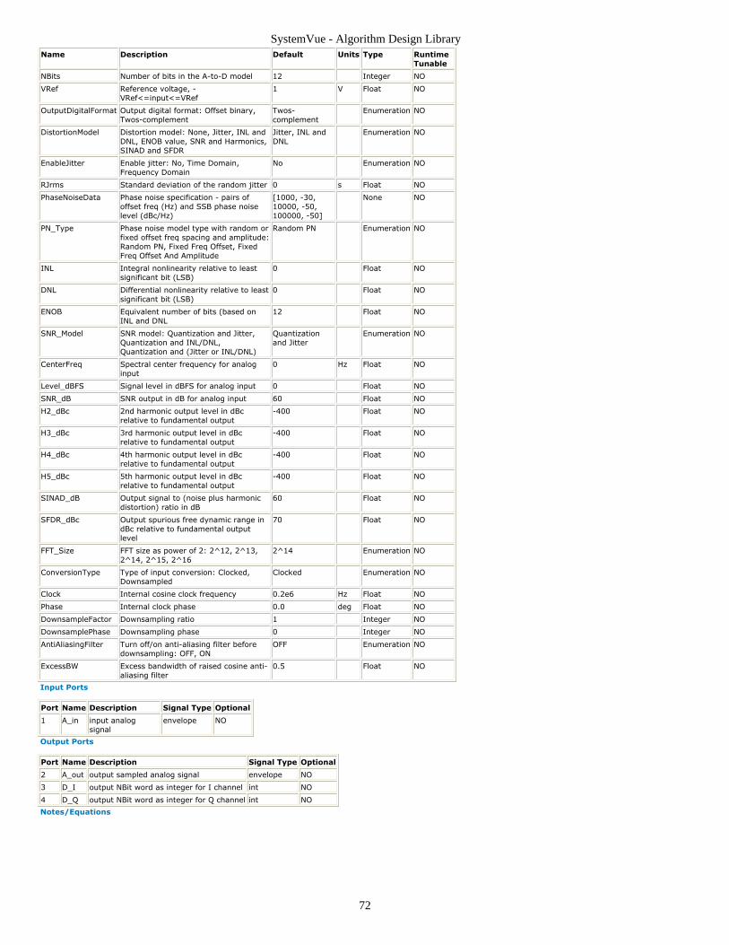
SystemVue - Algorithm Design Library
72
Name Description Default Units Type RuntimeTunable
NBits Number of bits in the A-to-D model 12 Integer NO
VRef Reference voltage, -VRef<=input<=VRef
1 V Float NO
OutputDigitalFormat Output digital format: Offset binary,Twos-complement
Twos-complement
Enumeration NO
DistortionModel Distortion model: None, Jitter, INL andDNL, ENOB value, SNR and Harmonics,SINAD and SFDR
Jitter, INL andDNL
Enumeration NO
EnableJitter Enable jitter: No, Time Domain,Frequency Domain
No Enumeration NO
RJrms Standard deviation of the random jitter 0 s Float NO
PhaseNoiseData Phase noise specification - pairs ofoffset freq (Hz) and SSB phase noiselevel (dBc/Hz)
[1000, -30,10000, -50,100000, -50]
None NO
PN_Type Phase noise model type with random orfixed offset freq spacing and amplitude:Random PN, Fixed Freq Offset, FixedFreq Offset And Amplitude
Random PN Enumeration NO
INL Integral nonlinearity relative to leastsignificant bit (LSB)
0 Float NO
DNL Differential nonlinearity relative to leastsignificant bit (LSB)
0 Float NO
ENOB Equivalent number of bits (based onINL and DNL
12 Float NO
SNR_Model SNR model: Quantization and Jitter,Quantization and INL/DNL,Quantization and (Jitter or INL/DNL)
Quantizationand Jitter
Enumeration NO
CenterFreq Spectral center frequency for analoginput
0 Hz Float NO
Level_dBFS Signal level in dBFS for analog input 0 Float NO
SNR_dB SNR output in dB for analog input 60 Float NO
H2_dBc 2nd harmonic output level in dBcrelative to fundamental output
-400 Float NO
H3_dBc 3rd harmonic output level in dBcrelative to fundamental output
-400 Float NO
H4_dBc 4th harmonic output level in dBcrelative to fundamental output
-400 Float NO
H5_dBc 5th harmonic output level in dBcrelative to fundamental output
-400 Float NO
SINAD_dB Output signal to (noise plus harmonicdistortion) ratio in dB
60 Float NO
SFDR_dBc Output spurious free dynamic range indBc relative to fundamental outputlevel
70 Float NO
FFT_Size FFT size as power of 2: 2^12, 2^13,2^14, 2^15, 2^16
2^14 Enumeration NO
ConversionType Type of input conversion: Clocked,Downsampled
Clocked Enumeration NO
Clock Internal cosine clock frequency 0.2e6 Hz Float NO
Phase Internal clock phase 0.0 deg Float NO
DownsampleFactor Downsampling ratio 1 Integer NO
DownsamplePhase Downsampling phase 0 Integer NO
AntiAliasingFilter Turn off/on anti-aliasing filter beforedownsampling: OFF, ON
OFF Enumeration NO
ExcessBW Excess bandwidth of raised cosine anti-aliasing filter
0.5 Float NO
Input Ports
Port Name Description Signal Type Optional
1 A_in input analogsignal
envelope NO
Output Ports
Port Name Description Signal Type Optional
2 A_out output sampled analog signal envelope NO
3 D_I output NBit word as integer for I channel int NO
4 D_Q output NBit word as integer for Q channel int NO
Notes/Equations

SystemVue - Algorithm Design Library
73
AtoD PartCategories: Analog/RF (algorithm)
The models associated with this part are listed below. To view detailed information on amodel (description, parameters, equations, notes, etc.), please click the appropriate link.
Model Description
AtoD(algorithm)
Analog to Digital Converter with Integral and Differential Nonlinearities
AtoD
Description: Analog to Digital Converter with Integral and Differential NonlinearitiesDomain: TimedC++ Code Generation Support: NOAssociated Parts: AtoD Part (algorithm)
Model Parameters

SystemVue - Algorithm Design Library
74
Name Description Default Units Type RuntimeTunable
Range
NBits Number of bits 8 Integer NO [4:16]
VRef Reference voltage, -VRef<=input<=VRef
1.0 V Float NO (0:∞)
OutputDigitalFormat Output digital format: Offset binary,Twos-complement
Offset binary Enumeration NO
DistortionModel Distortion model: None,Jitter/INL/DNL, ENOB value, SNRand Harmonics, SINAD and SFDR
Jitter/INL/DNL Enumeration NO
EnableJitter Enable jitter: No, Time Domain,Frequency Domain
No Enumeration NO
RJrms Standard deviation of random jitter 0.0 s Float NO [0:∞)
PhaseNoiseData Phase noise specification - pairs ofoffset freq (Hz) and SSB phase noiselevel (dBc/Hz)
Floatingpoint array
NO
PN_Type Phase noise model type with randomor fixed offset freq spacing andamplitude: Random PN, Fixed freqoffset, Fixed freq offset andamplitude
Random PN Enumeration NO
INL Integral nonlinearity relative to leastsignificant bit (LSB)
0.0 Float NO [DNL/2:∞)
DNL Differential nonlinearity relative toleast significant bit (LSB)
0.0 Float NO [0:∞)
ENOB Equivalent number of bits (based onINL and DNL)
7 Float NO [1:16]
SNR_dB SNR output in dB for analog input 60.0 Float NO (-∞:∞)
H2_dBc 2nd harmonic output level in dBcrelative to fundamental output
-400.0 Float NO (-ing:-10]
H3_dBc 3rd harmonic output level in dBcrelative to fundamental output
-400.0 Float NO (-ing:-10]
H4_dBc 4th harmonic output level in dBcrelative to fundamental output
-400.0 Float NO (-ing:-10]
H5_dBc 5th harmonic output level in dBcrelative to fundamental output
-400.0 Float NO (-ing:-10]
SINAD_dB Output signal to (noise plusharmonic distortion) ratio in dB
60.0 Float NO (-∞:∞)
SFDR_dBc Output spurious free dynamic rangein dBc relative to fundamentaloutput level
70.0 Float NO (-∞:∞)
FFT_Size FFT size as power of 2: 2^12, 2^13,2^14, 2^15, 2^16
2^14 Enumeration NO
SNR_Model SNR model: Quantization_and_Jitter,Quantization_and_INL_DNL,Quantization_and_Jitter_or_INL_DNL
Quantization_and_Jitter Enumeration NO
CenterFreq Spectral center frequency for analoginput
0.0 Hz Float NO [0.0:∞)
Level_dBFS Signal level in dBFS for analog input 0.0 Float NO (-∞:0.0]
ConversionType Type of input conversion: Clocked,Downsampled
Clocked Enumeration NO
Clock Internal cosine clock frequency 0.2e6 Hz Float NO (0:SR]†
Phase Internal clock phase 0.0 deg Float NO (-∞:∞)
DownsampleFactor Downsampling ratio 1 Integer NO [1:∞)
DownsamplePhase Downsampling phase 0 Integer NO [0:Factor-1]
AntiAliasingFilter Turn off/on anti-aliasing filter beforedownsampling: OFF, ON
OFF Enumeration NO
ExcessBW Excess bandwidth of raised cosineanti-aliasing filter
0.5 Float NO [0:1]
Input Ports
Port Name Description Signal Type Optional
1 A_in input analogsignal
envelope NO
Output Ports
Port Name Description Signal Type Optional
2 A_out output sampled analog baseband signal envelope NO
3 D_I output NBit word as integer for I channel int NO
4 D_Q output NBit word as integer for Q channel int NO
Notes/Equations
This model implements an analog-to-digital converter (ADC) with an internal clock1.and various distortion models.The input A_in can be a real baseband signal or a complex envelope signal.2.
When the input signal is a real baseband signal, it is sampled (with theappropriate jitter/phase noise and non-linear distortion applied) and quantized

SystemVue - Algorithm Design Library
75
(based on the NBits, VRef, INL, and DNL) to generate the real baseband outputsignal A_out. The bits that represent the quantized input signal value (the indexof the quantization level to which the input signal sample was quantized to) areoutput as an integer value at the port D_I. The signal at the port D_Q is always0.When the input signal is a complex envelope signal, its I and Q envelopes aresampled (with the appropriate jitter/phase noise and non-linear distortionapplied) and quantized (based on the NBits, VRef, INL, and DNL) to generate theI and Q envelopes of the output signal A_out. The characterization frequency ofA_out is the same as the characterization frequency of A_in. The bits thatrepresent the quantized values of the I and Q envelope of the input signal (theindices of the quantization levels to which the envelope values were quantizedto) are output as integer values at the ports D_I and D_Q respectively.
The NBits parameter sets the number of bits for the ADC. The number of quantization3.levels is 2NBits. The higher the number of bits the smaller the quantization error,which means that the output signal A_out matches the input A_in more closely.The VRef parameter sets the reference voltage for the ADC. The input signal must lie4.in the range [−Verf, VRef]. Otherwise, clipping occurs.The OutputDigitalFormat parameter sets the range of values for the D_I and D_Q5.outputs. If OutputDigitalFormat = Offset binary, then D_I and D_Q are integers inthe range [0, 2NBits−1]. If OutputDigitalFormat = Twos-complement, then D_I andD_Q are integers in the range [−2NBits−1, 2NBits−1−1]. The following graphs show theD_I output for an ideal 3-bit ADC with VRef = 1, when OutputDigitalFormat = Offsetbinary and OutputDigitalFormat = Twos-complement.
There are a number of ways to quantify the distortion and noise of an AtoD. All of6.them are based on an FFT analysis. Typical measurements include:
SNR (Signal to Noise Ratio) is the ratio of the rms value of the signal to themean value of the root-sum-square of all noise components (excluding dc andharmonics).
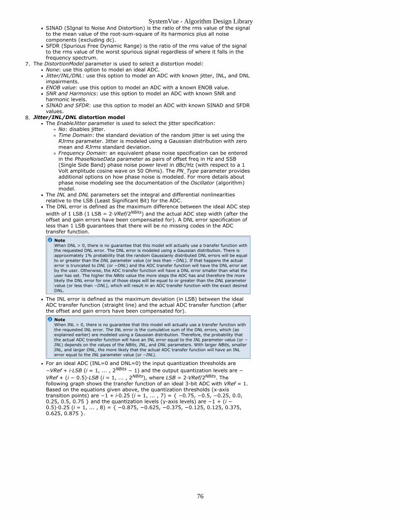
SystemVue - Algorithm Design Library
76
SINAD (SIgnal to Noise And Distortion) is the ratio of the rms value of the signalto the mean value of the root-sum-square of its harmonics plus all noisecomponents (excluding dc).SFDR (Spurious Free Dynamic Range) is the ratio of the rms value of the signalto the rms value of the worst spurious signal regardless of where it falls in thefrequency spectrum.
The DistortionModel parameter is used to select a distortion model:7.None: use this option to model an ideal ADC.Jitter/INL/DNL: use this option to model an ADC with known jitter, INL, and DNLimpairments.ENOB value: use this option to model an ADC with a known ENOB value.SNR and Harmonics: use this option to model an ADC with known SNR andharmonic levels.SINAD and SFDR: use this option to model an ADC with known SINAD and SFDRvalues.
Jitter/INL/DNL distortion model8.The EnableJitter parameter is used to select the jitter specification:
No: disables jitter.Time Domain: the standard deviation of the random jitter is set using theRJrms parameter. Jitter is modeled using a Gaussian distribution with zeromean and RJrms standard deviation.Frequency Domain: an equivalent phase noise specification can be enteredin the PhaseNoiseData parameter as pairs of offset freq in Hz and SSB(Single Side Band) phase noise power level in dBc/Hz (with respect to a 1Volt amplitude cosine wave on 50 Ohms). The PN_Type parameter providesadditional options on how phase noise is modeled. For more details aboutphase noise modeling see the documentation of the Oscillator (algorithm)model.
The INL and DNL parameters set the integral and differential nonlinearitiesrelative to the LSB (Least Significant Bit) for the ADC.The DNL error is defined as the maximum difference between the ideal ADC stepwidth of 1 LSB (1 LSB = 2·VRef/2NBits) and the actual ADC step width (after theoffset and gain errors have been compensated for). A DNL error specification ofless than 1 LSB guarantees that there will be no missing codes in the ADCtransfer function.
NoteWhen DNL > 0, there is no guarantee that this model will actually use a transfer function withthe requested DNL error. The DNL error is modeled using a Gaussian distribution. There isapproximately 1% probability that the random Gaussianly distributed DNL errors will be equalto or greater than the DNL parameter value (or less than −DNL). If that happens the actualerror is truncated to DNL (or −DNL) and the ADC transfer function will have the DNL error setby the user. Otherwise, the ADC transfer function will have a DNL error smaller than what theuser has set. The higher the NBits value the more steps the ADC has and therefore the morelikely the DNL error for one of those steps will be equal to or greater than the DNL parametervalue (or less than −DNL), which will result in an ADC transfer function with the exact desiredDNL.
The INL error is defined as the maximum deviation (in LSB) between the idealADC transfer function (straight line) and the actual ADC transfer function (afterthe offset and gain errors have been compensated for).
NoteWhen INL > 0, there is no guarantee that this model will actually use a transfer function withthe requested INL error. The INL error is the cumulative sum of the DNL errors, which (asexplained earlier) are modeled using a Gaussian distribution. Therefore, the probability thatthe actual ADC transfer function will have an INL error equal to the INL parameter value (or −INL) depends on the values of the NBits, INL, and DNL parameters. With larger NBits, smallerINL, and larger DNL, the more likely that the actual ADC transfer function will have an INLerror equal to the INL parameter value (or −INL).
For an ideal ADC (INL=0 and DNL=0) the input quantization thresholds are−VRef + i·LSB (i = 1, ... , 2NBits − 1) and the output quantization levels are −VRef + (i − 0.5)·LSB (i = 1, ... , 2NBits), where LSB = 2·VRef/2NBits. Thefollowing graph shows the transfer function of an ideal 3-bit ADC with VRef = 1.Based on the equations given above, the quantization thresholds (x-axistransition points) are −1 + i·0.25 (i = 1, ... , 7) = { −0.75, −0.5, −0.25, 0.0,0.25, 0.5, 0.75 } and the quantization levels (y-axis levels) are −1 + (i −0.5)·0.25 (i = 1, ... , 8) = { −0.875, −0.625, −0.375, −0.125, 0.125, 0.375,0.625, 0.875 }.

SystemVue - Algorithm Design Library
77
ENOB value distortion model9.The ENOB parameter is used to set the Equivalent Number Of Bits for the ADCmodel.The ENOB specification is first converted to an equivalent SNR specification,which depending on the value of the SNR_Model parameter is finally convertedto an equivalent Time Domain jitter or INL/DNL specification.
SNR and Harmonics distortion model10.The SNR_dB parameter is used to set the output Signal to Noise Ratio for theADC model.Depending on the value of the SNR_Model parameter the SNR_dB specificationis converted to an equivalent Time Domain jitter or INL/DNL specification.The H2_dBc, H3_dBc, H4_dBc, and H5_dBc parameters are used to specify theoutput levels of the 2nd, 3rd, 4th, and 5th harmonics in dBc (relative to thefundamental output level). A non-linear polynomial model is created based onthe values of these parameters. The non-linearity is applied to the input signalbefore any jitter or quantization effects are applied.
SINAD and SFDR distortion model11.The SINAD_dB parameter is used to set the output Signal to Noise and(harmonic) Distortion ratio for the ADC model.The SFDR_dBc parameter is used to set the output Spurious Free DynamicRange in dBc (relative to fundamental output level) for the ADC model.The FFT_Size parameter is used to set the size of the FFT used when measuringthe SFDR of the ADC model. For the SFDR measurement, the worst spur mightnot be a harmonic of the original signal and may be close to the FFT noise floor.Since the noise floor in the FFT is dependent on size of the FFT, this distortionmodel requires that the FFT size be specified, so that the SFDR can be properlymodeled.The SINAD_dB and SFDR_dBc specifications are converted to an equivalent SNRand Harmonics specification.
When DistortionModel is set to ENOB value, SNR and Harmonics, or SINAD and SFDR,12.the SNR_Model parameter is used to specify how the SNR, whether explicitly set (SNR and Harmonics case) or inferred (ENOB value and SINAD and SFDR cases), isgoing to be modeled. The SNR contributors are quantization noise, jitter, andINL/DNL.
Quantization_and_Jitter: SNR is modeled through quantization noise and jitter.Quantization_and_INL_DNL: SNR is modeled through quantization noise andINL/DNL.Quantization_and_Jitter_or_INL_DNL: SNR is modeled through quantizationnoise and jitter or INL/DNL (whichever is more appropriate).
The CenterFrequency parameter sets the spectral center frequency of the analog13.input signal. This is used to compute SNR lower limits and appropriately decide howto model SNR.The Level_dBFS parameter sets the level in dBFS (dB Full Scale) for the analog input14.signal.This ADC model can operate in two different modes: Clocked and Downsampled15.(specified in the ConversionType parameter)
In the Clocked mode, the model reads one sample from its input and writesone sample to each of its outputs. The internal clock frequency (Clockparameter) and phase (Phase parameter) need to be set. The internal clock is ofthe form cos( 2·π·Clock·t + Phase ). The input signal is sampled at the positivezero crossings of the clock. To be able to detect zero crossings, at least foursamples per clock period are needed. Therefore, when SR/4 < Clock ≤ SR, theinternal clock is represented at 4·SR (SR is the sampling rate of the inputsignal). This does not affect the output signal sampling rate, which is always the

SystemVue - Algorithm Design Library
78
same as the input signal sampling rate (SR). Once the input signal is sampled,the sampled value is quantized and held constant at the output until the nextclock positive zero crossing occurs. If Clock < SR/2, the output will have theform of a piece wise constant waveform because of the sample and holdoperation. A piece wise constant waveform can show at the output even whenClock = SR. This is the case when NBits is not big enough, which can result inmultiple input signal values being quantized to the same output quantizationlevel.In the Downsampled mode, the DownsampleFactor and DownsamplePhaseparameters need to be set. In this case, the model reads DownsampleFactorsamples from its input and writes 1 sample to each of its outputs. The samplewritten to the outputs is the quantized DownsamplePhase-th sample in the blockof DownsampleFactor input samples. No explicit clock signal is used but theequivalent clock signal is cos( 2·π·SR·t/DownsampleFactor + 2·π·DownsamplePhase/DownsampleFactor − π/2 ). Since the input signal isdownsampled, the output signal will not have the form of a piece wise constantwaveform (no sample and hold operation), unless NBits is not big enough, whichcan result in multiple input signal values being quantized to the same outputquantization level.When downsampling a signal, aliasing can occur (if the sampling rate of thedownsampled signal is not high enough to represent the frequency content ofthe original signal). Therefore, a raised cosine antialiasing filter can be set up(set AntiAliasingFilter parameter to ON). The ExcessBW (or roll off factor) of thisfilter can also be specified. If the antialiasing filter is used a delay is introducedin the output signals.
For more details on downsampling see the documentation of the DownSampleEnv (algorithm)model.
The internal clock whether explicit (Clocked mode) or implicit (Downsampledmode) is impaired with jitter (when DistortionModel is set to Jitter/INL/DNL andEnableJitter is set to Timed Domain or when an equivalent jitter is calculatedfrom the other distortion models) or phase noise (when DistortionModel is set toJitter/INL/DNL and EnableJitter is set to Frequency Domain). Jitter or phasenoise affect the clock zero crossings and therefore the instant the input signalgets sampled.When jitter is used and
ConversionType = Clocked, then 3·RJrms, where RJrms is the random jitterstandard deviation (explicitly set when DistortionModel is set toJitter/INL/DNL and EnableJitter is set to Timed Domain or inferred for theother distortion models), has to be smaller than 1/4 of the clock time step(note that when SR/4 < Clock ≤ SR, the clock time step is 1/4 of the inputsignal time step).ConversionType = Downsampled, then 3·RJrms has to be smaller than 1/2of the input signal time step.If the generated random jitter value happens to be outside the range [−3·RJrms, 3·RJrms] it gets limited to ±3·RJrms. Note that 99.7% of aGaussian distribution lies within 3·σ of its mean.
When phase noise is used andConversionType = Clocked, the phase noise error introduced cannot begreater (in absolute value) than the clock phase increment correspondingto 1/4 of the clock time step (note that when SR/4 < Clock ≤ SR, the clocktime step is 1/4 of the input signal time step).ConversionType = Downsampled, the phase noise error introduced cannotbe greater (in absolute value) than the clock phase incrementcorresponding to 1/2 of the input signal time step.If the generated phase noise error value happens to be outside the rangesmentioned above it gets limited to the upper or lower limits of theacceptable ranges.

SystemVue - Algorithm Design Library
79
CommsChannel PartCategories: Analog/RF (algorithm), Communications (algorithm)
The models associated with this part are listed below. To view detailed information on amodel (description, parameters, equations, notes, etc.), please click the appropriate link.
Model Description
CommsChannel(algorithm)
Wireless ChannelModel
CommsChannel
Description: Wireless Channel ModelDomain: TimedC++ Code Generation Support: NOAssociated Parts: CommsChannel Part (algorithm)
Model Parameters
Name Description Default Units Type RuntimeTunable
Range
ModelType Channel model type:UserDefined, Pedestrian_A,Pedestrian_B, Vehicular_A,Vehicular_B,Extended_Pedestrian_A,Extended_Vehicular_A,Extended_TypicalUrban
UserDefined Enumeration NO
Delay User defined tap delays in usec [0.0 , 0.03,0.15, 0.31,0.37, 0.71 ,1.09 , 1.73 ,2.51]
Floatingpoint array
NO [0:10000.0]
Power User defined relative tap powersin dB
[0.0, -1.5, -1.4, -3.6, -0.6, -9.1, -7.0, -12.0, -16.9]
Floatingpoint array
NO (-∞:0]
RiceanFactor User defined tap Ricean K-factors in linear scale
[0.0, 0.0, 0.0,0.0, 0.0, 0.0,0.0, 0.0, 0.0]
Floatingpoint array
NO [0.0:1000.0]
Velocity Velocity of mobile station inkm/hour
120 Float NO [0.001:1000]
PathLoss Include large-scale pathloss:NO, YES
NO Enumeration NO
PropDistance Distance between the transmitand receive stations
1000 m Float NO [200:5000]
PwrNormal Normalize output power: NO,YES
NO Enumeration NO
PwrMeasPeriod Power measurement time periodfor output power normalization
0.001 s Float NO (0:∞)
Input Ports
Port Name Description Signal Type Optional
1 input channel inputsignal
envelope NO
Output Ports
Port Name Description Signal Type Optional
2 output channel output signal envelope NO
3 tap fading channel complex tapcoefficients
multiple complex NO
Notes/Equations
This model is used to generate channel models for mobile wireless applications.1.This model reads 1 sample at its input and writes 1 sample at all outputs.2.Model use of Velocity, PropDistance, PathLoss, PwrNormal and PwrMeasPeriod3.Velocity specifies the mobile's velocity relative to base station.PropDistance specifies the distance between base station and mobile station.PathLoss identifies whether the large-scale pathloss is included.If PathLoss = NO, then the path loss is not included in this model and the parametersdescribing the environment are unused.

SystemVue - Algorithm Design Library
80
If PathLoss = YES, then the path loss for both urban and suburban environments ismodeled by the COST 207 model with a correction term. There are three terms whichmake up the model:The Path Loss model for outdoor to indoor and pedestrian test environment is,
where R is the propagation distance and f is the frequency.The Path Loss model for vehicular test environment is,
where R is the propagation distance and f is the frequency, is the height betweenbase station antenna and mobile.PwrNormal specifies whether the ouput power is normalized to the input power.When PwrNormal = YES, then the output power is normalized using thePwrMeasPeriod which is the time period for measuring power to ensure that theoutput power is equal to the input power with the resolution of PwrMeasPeriod. Themethod for adjusting the ouput power is that, assuming the power level measured intwo contiguous time periods with PwrMeasPeriod seconds is identical, a gain,calculated on the power level measured in the (i-1)th time period, is multiplied to thesignal in the ith time period to ensure that the output power in the ith time period isequal to the input power, and so on for the (i+1)th time period. Hence the first timeperiod with PwrMeasPeriod seconds remain unadjusted.Channel model definition when ModelType = Extended_Pedestrian_A,4.Extended_Vehicular_A, Extended_TypicalUrbanThis model is implemented following the channel model requirements defined for3GPP LTE mobile wireless applications and based onR4-070872 3GPP TR36.803v0.3.0. See references 1 and 2 below.For this model, the Delay, Power and RiceanFactor are predefined and not userspecifiable.For this model a delay of 64 tokens is introduced in the outputs.A set of 3 channel models are implemented to simulate the multipath fadingpropagation conditions. The multipath fading is modeled as a tapped-delay line with anumber of taps at fixed positions on a sampling grid. The gain associated with eachtap is characterized by a distribution (Ricean with a K-factor>0, or Rayleigh with K-factor=0) and the maximum Doppler frequency that is determined from the mobilespeed. For each tap, the method of filtered noise is used to generate channelcoefficients with the specified distribution and spectral power density.The definition of the 3 specific channels are shown in the following tables:Extended Pedestrian A model (EPA)Tap Excess tap delay [ns] Relative power [dB]
1 0 0.0
2 30 -1.0
3 70 -2.0
4 90 -3.0
5 110 -8.0
6 190 -17.2
7 410 -20.8
Extended Vehicular A model (EVA)
Tap Excess tap delay [ns] Relative power [dB]
1 0 0.0
2 30 -1.5
3 150 -1.4
4 310 -3.6
5 370 -0.6
6 710 -9.1
7 1090 -7.0
8 1730 -12.0
9 2510 -16.9
Extended Typical Urban model (ETU)
Tap Excess tap delay [ns] Relative power [dB]
1 0 -1.0
2 50 -1.0
3 120 -1.0
4 200 -0.0
5 230 -0.0
6 500 -0.0
7 1600 -3.0
8 2300 -5.0
9 5000 -7.0
The total channel gain is normalized by adding the specified Normalization Factor toeach tap.The Doppler spectrum is modelled using the well known Clarke or Classical Doppler

SystemVue - Algorithm Design Library
81
spectrum. The power spectral density (PSD) function is defined as follows: !3gpplte-channel-2008-1-01.gif! where !3gpplte-channel-2008-1-02.gif! is the net power, and!3gpplte-channel-2008-1-03.gif! denotes the maximum Doppler frequency, and!3gpplte-channel-2008-1-04.gif! where !3gpplte-channel-2008-1-06.gif! is the speedof the mobile, !3gpplte-channel-2008-1-05.gif! is the carrier frequency and c is thespeed of light.Channel model definition when ModelType = Pedestrian_A, Pedestrian_B,5.Vehicular_A, Vehicular_BThis model is implemented following Rec.ITU-R M.1225 for mobile wirelessapplications. See references 3 below.For this model, the Delay, Power and RiceanFactor are predefined and not userspecifiable.For this model a delay of 64 tokens is introduced in the outputs.A set of 4 modified International Telecommunication Union (ITU) channel models areconstructed to simulate the multipath fading of the channel. The multipath fading ismodeled as a tapped-delay line with 6 taps with non-uniform delays. The gainassociated with each tap is characterized by a distribution (Ricean with a K-factor>0,or Rayleigh with K-factor=0) and the maximum Doppler frequency. For each tap, themethod of filtered noise is used to generate channel coefficients with the specifieddistribution and spectral power density.The definition of the 4 specific ITU channels is shown in the following tables:
Outdoor to Indoor and Pedestrian Test Environment Tapped-Delay-Line Parameters
Tap Channel A Channel B DopplerSpectrum
Relative Delay(ns)
Average Power(dB)
Relative Delay(ns)
Average Power(dB)
1 0 0 0 0 Classic
2 110 -9.7 200 -0.9 Classic
3 190 -19.2 800 -4.9 Classic
4 410 -22.8 1200 -8.0 Classic
5 °™°™ °™°™ 2300 -7.8 Classic
6 °™°™ °™°™ 3700 -23.9 Classic
Vehicular Test Environment Tapped-Delay-Line Parameters
Tap Channel A Channel B DopplerSpectrum
Relative Delay(ns)
Average Power(dB)
Relative Delay(ns)
Average Power(dB)
1 0 0.0 0 -2.5 Classic
2 310 -1.0 300 0 Classic
3 710 -9.0 8900 -12.8 Classic
4 1090 -10.0 12900 -10.0 Classic
5 1730 -15.0 17100 -25.2 Classic
6 2510 -20.0 20000 -16.0 Classic
The total channel gain is normalized by adding the specified Normalization Factor toeach tap.The specified Doppler is the maximum Doppler frequency parameter (fm) of therounded spectrum which has the power spectral density (PSD) function as follows:
where and , is the mobile's velocity relative to base station.The set of ITU channel models specify statistical parameters of microscopic effects.To simulate the real channel, these statistics have to be combined with macroscopicchannel effects, i.e. the path loss (including shadowing) which will be introduced inthe later section.The COST 207 model with a correction term is used to simulate the path loss for bothpedestrian and vehicular environments if the PathLoss is ON and other parametersare set according to the specific environment.Channel model definition when ModelType = UserDefined6.For this model, the Delay, Power and RiceanFactor array values specified are used todefine the model. These three arrays must has the same size. This size defines Ntaps in a tapped-delay line. The multipath fading model follows the same approachfor the above predefined models, but with user defined characteristics. The multipathfading is modeled as a tapped-delay line with N taps with the delays ( Delay ) andgains ( Power ) specified. Each gain will have a distribution defined by the theRiceanFactor (Ricean when RiceanFactor > 0, or Rayleigh when RiceanFactor = 0)and the maximum Doppler frequency. For each tap, we use the method of filterednoise to generate channel coefficients with the specified distribution and spectralpower density.

SystemVue - Algorithm Design Library
82
References
Rec.ITU-R M.1225, Guidelines For Evaluation Of Radio Transmission Technologies For1.IMT-2000, 1997.3GPP TS 36.104 v8.1.0, User Equipment (UE) radio transmission and reception,2.2008-03.Rec.ITU-R M.1225, Guidelines For Evaluation Of Radio Transmission Technologies For3.IMT-2000, 1997 .

SystemVue - Algorithm Design Library
83
CommsMIMO_Channel PartCategories: Analog/RF (algorithm), Communications (algorithm)
The models associated with this part are listed below. To view detailed information on amodel (description, parameters, equations, notes, etc.), please click the appropriate link.
Model Description
LTE_MIMO_Channel(algorithm)
LTE MIMO ChannelModel
LTE_MIMO_Channel
Description: LTE MIMO Channel ModelDomain: TimedC++ Code Generation Support: NOAssociated Parts: CommsMIMO Channel Part (algorithm)
Model Parameters
Name Description Default Units Type RuntimeTunable
Range
AntennaConfig Antenna configuration as(number of Tx) x (numberof Rx) antennas: TR_1x2,TR_2x2, TR_4x2, TR_4x4,TR_4x1, TR_2x1, TR_2x4,TR_1x4, TR_1x8, TR_2x8,TR_4x8, TR_8x1, TR_8x2,TR_8x4, TR_8x8
TR_2x2 Enumeration NO
CorrelationType MIMO channel correlationmatrix type: Low, Medium,High
Low Enumeration NO
CorrMatrix_I_FileName The filename of Correlationmatrix real part
Filename NO
CorrMatrix_Q_FileName The filename of Correlationmatrix imag part
Filename NO
ModelType Channel model type:UserDefined,Extended_Pedestrian_A,Extended_Vehicular_A,Extended_TypicalUrban
UserDefined Enumeration NO
Delay User defined tap delays inusec
[0.0 , 0.03,0.15, 0.31,0.37, 0.71 ,1.09 , 1.73 ,2.51]
Floatingpoint array
NO [0:10000.0]
Power User defined relative tappowers in dB
[0.0, -1.5, -1.4, -3.6, -0.6, -9.1, -7.0, -12.0, -16.9]
Floatingpoint array
NO (-∞:0]
RiceanFactor User defined tap Ricean K-factors in linear scale
[0.0, 0.0,0.0, 0.0,0.0, 0.0,0.0, 0.0,0.0]
Floatingpoint array
NO [0.0:1000.0]
Velocity Velocity of mobile stationin km/hour
120 Float NO [0.001:1000]
Input Ports
Port Name Description Signal Type Optional
1 TxSig Signals supplied to transmit array multipleenvelope
NO
Output Ports
Port Name Description Signal Type Optional
2 RxSig Signals at output of receivearray
multipleenvelope
NO
Notes/Equations
The model implements a MIMO channel as defined for 3GPP LTE wireless systems and1.follows the definition in B.2 of 36.101 [1].This model reads 1 sample from the inputs and writes 1 sample to the outputs.2.
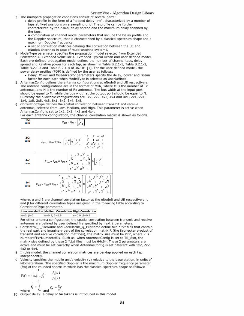
SystemVue - Algorithm Design Library
84
The multipath propagation conditions consist of several parts:3.delay profile in the form of a "tapped delay-line", characterized by a number oftaps at fixed positions on a sampling grid. The profile can be furthercharacterized by the r.m.s. delay spread and the maximum delay spanned bythe taps.A combination of channel model parameters that include the Delay profile andthe Doppler spectrum, that is characterized by a classical spectrum shape and amaximum Doppler frequencyA set of correlation matrices defining the correlation between the UE andeNodeB antennas in case of multi-antenna systems.
ModelType parameter specifies the propagation model selected from Extended4.Pedestrian A, Extended Vehicular A, Extended Typical Urban and user-defined model.Each pre-defined propagation model defines the number of channel taps, delayspread and Relative power for each tap, as shown in Table B.2.1-1, Table B.2.1-2,Table B.2.1-3 and Table B.2.1-4 of 36.101 [1]. For the user-defined model, thepower delay profiles (PDP) is defined by the user as follows:
Delay, Power and RiceanFactor parameters specify the delay, power and riceanfactor for each path when ModelType is selected as UserDefined.
AntennasConfig defines the antenna configurations at eNodeB and UE respectively.5.The antenna configurations are in the format of MxN, where M is the number of Txantennas, and N is the number of Rx antennas. The bus width at the input portshould be equal to M, while the bus width at the output port should be equal to N.Currently the allowable configurations are 1x2, 2x2, 4x2, 4x4 and 4x1, 2x1, 2x4,1x4, 1x8, 2x8, 4x8, 8x1, 8x2, 8x4, 8x8.CorrelationType defines the spatial correlation between transmit and receive6.antennas, selected from Low, Medium, and High. This parameter is active whenAntennasConfig is set to 1x2, 2x2, 4x2 and 4x4.For each antenna configuration, the channel correlation matrix is shown as follows,
where, α and β are channel correlation factor at the eNodeB and UE respectively. αand β for different correlation types are given in the following table according toCorrelationType parameter.Low correlation Medium Correlation High Correlation
α=0, β=0 α=0.3, β=0.9 α=0.9, β=0.9
For other antenna configuration, the spatial correlation between transmit and receiveantennas are defined by user defined file specified by next 2 parameters.CorrMatrix_I_FileName and CorrMatrix_Q_FileName define two *.txt files that contain7.the real part and imaginary part of the correlation matrix R (the Kronecker product oftransmit and receive correlation matrices), the matrix size must be KxK, where K isNumberofTx*NumberofRx. Such as, when AntennasConfig is set to TR_8x8, thematrix size defined by these 2 *.txt files must be 64x64. These 2 parameters areactive and must be set correctly when AntennasConfig is set different with 1x2, 2x2,4x2 or 4x4.In this model, the channel correlation matrices are per-tap applied on each tap8.independently.Velocity specifies the mobile unit's velocity (ν) relative to the base station, in units of9.kilometer/hour. The specified Doppler is the maximum Doppler frequency parameter(fm) of the rounded spectrum which has the classical spectrum shape as follows:
where and .Output delay: a delay of 64 tokens is introduced in this model10.

SystemVue - Algorithm Design Library
85
References
3GPP TS 36.101 v8.5.1 "User Equipment (UE) radio transmission and reception",1.March 2009.
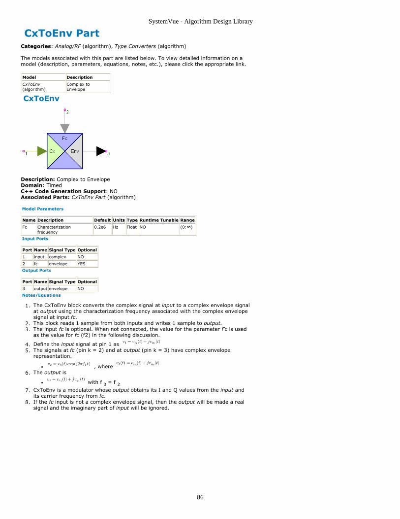
SystemVue - Algorithm Design Library
86
CxToEnv PartCategories: Analog/RF (algorithm), Type Converters (algorithm)
The models associated with this part are listed below. To view detailed information on amodel (description, parameters, equations, notes, etc.), please click the appropriate link.
Model Description
CxToEnv(algorithm)
Complex toEnvelope
CxToEnv
Description: Complex to EnvelopeDomain: TimedC++ Code Generation Support: NOAssociated Parts: CxToEnv Part (algorithm)
Model Parameters
Name Description Default Units Type Runtime Tunable Range
Fc Characterizationfrequency
0.2e6 Hz Float NO (0:∞)
Input Ports
Port Name Signal Type Optional
1 input complex NO
2 fc envelope YES
Output Ports
Port Name Signal Type Optional
3 output envelope NO
Notes/Equations
The CxToEnv block converts the complex signal at input to a complex envelope signal1.at output using the characterization frequency associated with the complex envelopesignal at input fc.This block reads 1 sample from both inputs and writes 1 sample to output.2.The input fc is optional. When not connected, the value for the parameter Fc is used3.as the value for fc (f2) in the following discussion.
Define the input signal at pin 1 as 4.The signals at fc (pin k = 2) and at output (pin k = 3) have complex envelope5.representation.
, where The output is6.
with f 3 = f 2CxToEnv is a modulator whose output obtains its I and Q values from the input and7.its carrier frequency from fc.If the fc input is not a complex envelope signal, then the output will be made a real8.signal and the imaginary part of input will be ignored.
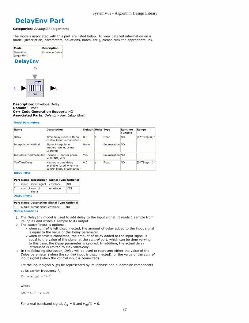
SystemVue - Algorithm Design Library
87
DelayEnv PartCategories: Analog/RF (algorithm)
The models associated with this part are listed below. To view detailed information on amodel (description, parameters, equations, notes, etc.), please click the appropriate link.
Model Description
DelayEnv(algorithm)
Envelope Delay
DelayEnv
Description: Envelope DelayDomain: TimedC++ Code Generation Support: NOAssociated Parts: DelayEnv Part (algorithm)
Model Parameters
Name Description Default Units Type RuntimeTunable
Range
Delay Time delay (used with nocontrol input is connected)
0.0 s Float NO [0*TStep:∞)†
InterpolationMethod Signal interpolationmethod: None, Linear,Lagrange
None Enumeration NO
IncludeCarrierPhaseShift Include RF carrier phaseshift: NO, YES
YES Enumeration NO
MaxTimeDelay Maximum time delayavailable (used when thecontrol input is connected)
0.0 s Float NO [0*TStep:∞)†
Input Ports
Port Name Description Signal Type Optional
1 input input signal envelope NO
2 control controlsignal
envelope YES
Output Ports
Port Name Description Signal Type Optional
3 output output signal envelope NO
Notes/Equations
The DelayEnv model is used to add delay to the input signal. It reads 1 sample from1.its inputs and writes 1 sample to its output.The control input is optional.2.
when control is left disconnected, the amount of delay added to the input signalis equal to the value of the Delay parameter.when control is connected, the amount of delay added to the input signal isequal to the value of the signal at the control port, which can be time varying.In this case, the Delay parameter is ignored. In addition, the actual delayintroduced is limited to MaxTimeDelay.
In the following discussion, Delay will be used to represent either the value of the3.Delay parameter (when the control input is disconnected), or the value of the controlinput signal (when the control input is connected).
Let the input signal V1(t) be represented by its inphase and quadrature components
at its carrier frequency fc1
where
For a real baseband signal, fc1 = 0 and vQ1(t) = 0.

SystemVue - Algorithm Design Library
88
The output signal V3(t) is represented by its inphase and quadrature components at
its carrier frequency fc3
where
fc3 = fc1v3(t) = v1(t - Delay), when IncludeCarrierPhaseShift is set to No
v3(t) = v1(t - Delay)·e-j2π·fc3
·Delay, when IncludeCarrierPhaseShift is set to Yes
When InterpolationMethod is set to linear or Lagrange, v1(t - Delay) is found using
the corresponding interpolation method.When InterpolationMethod is set to none, v1(t - Delay) is found using a 0th-order
interpolation method that maps v1(t - Delay) to the closest existing sample (see
graph below).
When the input signal is a real baseband signal (fc1 = 0), the4.
IncludeCarrierPhaseShift parameter has no effect on the output signal, since e-j2π·fc3
·Delay = 1.When InterpolationMethod is Lagrange and Delay is less than 2·Ts (where Ts is the5.
input signal simulation time step), then Linear interpolation is used.

SystemVue - Algorithm Design Library
89
Demodulator PartCategories: Analog/RF (algorithm), Communications (algorithm)
The models associated with this part are listed below. To view detailed information on amodel (description, parameters, equations, notes, etc.), please click the appropriate link.
Model Description
Demodulator(algorithm)
Demodulator
Demodulator (Demodulator)
Description: DemodulatorDomain: TimedC++ Code Generation Support: NOAssociated Parts: Demodulator Part (algorithm)
Model Parameters
Name Description Default Units Type RuntimeTunable
Range Symbol
OutputType Output type: I/Q,Amp/Phase, Amp/Freq
I/Q Enumeration NO
FCarrier Carrier frequency 0.2e6 Hz Float NO (0:∞) fc
InitialPhase Initial phase 0 deg Float NO (-∞:∞)
θ
AmpSensitivity Amplitude sensitivity 1 Float NO (-∞:∞)
Sa
PhaseSensitivity Phase deviationsensitivity in Volts/degree
1.0/90.0 Float NO (-∞:∞)
Sp
FreqSensitivity Frequency deviationsensitivity in Volts/Hz
1.0e-4 Float NO (-∞:∞)
Sf
MirrorSignal Mirror signal aboutcarrier: NO, YES
NO Enumeration NO
ShowIQ_Impairments Show I and Qimpairments: NO, YES
NO Enumeration NO
GainImbalance Gain imbalance in dB 0.0 Float NO (-∞:∞)
G
PhaseImbalance Phase imbalance 0.0 deg Float NO (-∞:∞)
φ
I_OriginOffset I origin offset 0.0 Float NO (-∞:∞)
Ioff
Q_OriginOffset Q origin offset 0.0 Float NO (-∞:∞)
Qoff
IQ_Rotation IQ rotation 0.0 deg Float NO (-∞:∞)
R
Input Ports
Port Name Description Signal Type Optional
1 input complex envelope vectorinput
envelope NO
Output Ports
Port Name Description Signal Type Optional
2 output1 output1 real NO
3 output2 output2 real NO
Notes/Equations
The Demodulator model implements a coherent demodulator that can be used to1.perform amplitude, phase, frequency, or I/Q demodulation.This model reads one sample from its input and writes one sample to its outputs.2.The input signal must be a complex envelope signal with characterization frequency3.greater than zero. Real input signals will result in a simulation error. If use with areal signal is needed, then the input to this model can be preceded with anEnvFcChange (algorithm) model that will recharacterize a real signal to itsrepresentation at a specified frequency.Let's assume that the complex envelope input signal is cx = I(t) + j·Q(t) at a4.characterization frequency of f1, which represents the real signal I(t)·cos( 2πf1t ) −
Q(t)·sin( 2πf t ).

SystemVue - Algorithm Design Library
90
1
First the InitialPhase is applied to the input signal by rotating it by −θ ( cx = cx·(5.cos(θ) − j·sin(θ) ).Then cx is recharacterized at fc.6.
See the documentation for EnvFcChange (algorithm) for detail on how a signal isconverted from one characterization frequency to another.The following discussion is in context with the input signal after it has beencharacterized at fc, that is, cx now represents the new complex envelope at fc.
Then the IQ impairments are applied to the input.7.I_OriginOffset and Q_OriginOffset: cx = cx + (Ioff + j·Qoff)
IQ_Rotation: cx = cx·( cos(R)+j·sin(R) )GainImbalance and PhaseImbalance: This model uses a symmetricimplementation of the imbalances. LetgI = 100.5·G/20
gQ = 10−0.5·G/20
φI = −φ/2
φQ = φ/2
The I and Q envelopes of the signal I(t)·cos( 2πfct ) − Q(t)·sin( 2πfct ) can be
recovered by multiplying it with cos( 2πfct ) and −sin( 2πfct ) respectively and
filtering the generated products at 2·fc. When the imbalances are applied, the
local oscillator for the I channel is not cos( 2πfct ) but gI · cos( 2πfct + φI ) and
the local oscillator for the Q channel is not −sin( 2πfct ) but −gQ · sin( ωc · t + φQ
).Recovered I[ I(t) · cos( 2πfct ) − Q(t) · sin( 2πfct ) ] · gI · cos( 2πfct + φI ) =
gI · I(t) · cos( 2πfct + φI ) · cos( 2πfct ) − gI · Q(t) · cos( 2πfct + φI ) · sin( 2πfct
) =Using the trig equationscos(a) · cos(b) = [ cos(a + b) + cos(a − b) ] / 2sin(a) · cos(b) = [ sin(a + b) + sin(a − b) ] / 2we get0.5 · gI · I(t) · [ cos( 2π·2·fct + φI ) + cos( φI ) ] − 0.5 · gI · Q(t) · [ sin( 2π·2·fct + φI ) + sin( −φI ) ] =
Omitting the terms at 2·fc, which can be filtered out, we get
0.5 · gI · I(t) · cos( φI ) − 0.5 · gI · Q(t) · sin( −φI ) =
0.5 · gI · [ I(t) · cos( φI ) − Q(t) · sin( −φI ) ] =
0.5 · gI · [ I(t) · cos( φI ) + Q(t) · sin( φI ) ]
This model ignores the scale factor of 0.5.Recovered Q−[ I(t) · cos( 2πfct ) − Q(t) · sin( 2πfct ) ] · gQ · sin( 2πfct + φQ ) =
−gQ · I(t) · sin( 2πfct + φQ ) · cos( 2πfct ) + gQ · Q(t) · sin( 2πfct + φQ ) · sin(
2πfct ) =
Using the trig equationssin(a) · sin(b) = [ cos(a − b) − cos(a + b) ] / 2sin(a) · cos(b) = [ sin(a + b) + sin(a − b) ] / 2we get−0.5 · gQ · I(t) · [ sin( 2π·2·fct + φQ ) + sin( φQ ) ] + 0.5 · gQ · Q(t) · [ cos( φQ
) − cos( 2π·2·fct + φQ ) ] =
Omitting the terms at 2·fc, which can be filtered out, we get
−0.5 · gQ · I(t) · sin( φQ ) + 0.5 · gQ · Q(t) · cos( φQ ) =
0.5 · gQ · [ −I(t) · sin( φQ ) + Q(t) · cos( φQ ) ]
This model ignores the scale factor of 0.5.If MirrorSignal = YES, then cx = conjugate( cx)8.Finally, the output is calculated as follows (in the following equations, I(t) and Q(t)9.represent the I and Q envelopes of the signal after all the transformations andimpairments described above have been applied):
When OutputType is set to I/Q,
When OutputType is set to Amp/Phase,
When OutputType is set to Amp/Frequency,

SystemVue - Algorithm Design Library
91
See also: Modulator (algorithm)10.

SystemVue - Algorithm Design Library
92
DownSampleEnv PartCategories: Analog/RF (algorithm), Routers/Resamplers (algorithm)
The models associated with this part are listed below. To view detailed information on amodel (description, parameters, equations, notes, etc.), please click the appropriate link.
Model Description
DownSampleEnv(algorithm)
Down Sampler for Envelope Signal
DownSampleEnv
Description: Down Sampler for Envelope SignalDomain: TimedC++ Code Generation Support: NOAssociated Parts: DownSampleEnv Part (algorithm)
Model Parameters
Name Description Default Units Type RuntimeTunable
Range
Factor Downsampling ratio 2 Integer NO [1:∞)
Phase Downsampling phase 0 Integer NO [0:Factor-1]
AntiAliasingFilter Turn off/on anti-aliasing filter beforedownsampling: OFF, ON
OFF Enumeration NO
ExcessBW Excess bandwidth of raised cosineanti-aliasing filter
0.5 Float NO [0:1]
Input Ports
Port Name Description Signal Type Optional
1 input input signal envelope NO
Output Ports
Port Name Description Signal Type Optional
2 output output signal envelope NO
To avoid confusion on a schematic, it is best to mirror (flip) this symbol (instead of rotating it) when youneed to have the input on the right and the output on the left of the symbol; otherwise the symbol arrowwill point in the "wrong" direction. Select the part and press F6 to flip the symbol into the correctorientation.
Notes/Equations
This component downsamples an input timed signal to produce an output timed1.signal sampled with a time step that is Factor times the input time step.This model reads Factor samples from the input and writes 1 sample to the output.2.The Phase parameter identifies which one of the Factor input sample is to be used as3.the output sample.Let N1 = the Nth input sample (starting at count of zero).Then, TIn = TStartIn + N1*TStepIn where TStartIn is the time stamp for the firstsample into this model.Let N2 = the Nth output sample (starting at count of zero) with one output sampleoccuring for every Factor input samples.Then, TOut = TStartOut + N2*TStepOut where TStartOut = TStartIn +Phase*TStepIn and TStepOut = Factor * TStepInv 2 (TOut) = v 1 (TOut)
The AntiAliasingFilter parameter can be used to activate/de-activate an anti-aliasing4.filter before downsampling. When the input signal is baseband, the anti-aliasing filteris a lowpass raised-cosine filter with bandwidth equal to 1/(2 × TStepOut). When theinput signal is a complex envelope signal, the anti-aliasing filter is a bandpass raised-cosine filter with bandwidth equal to 1/TStepOut. In both cases the filter has20 × Factor taps (it introduces a delay of 10 × TStepOut) and its excess bandwidthcan be set by the ExcessBW parameter.To downsample a signal by a non-integer factor, a cascade of an upsampler and5.downsampler is needed. For example, to change the sampling rate of a signal from73MHz (TStep = 13.69863 nsec) to 40MHz (TStep = 25 nsec), first pass it throughthe UpSampleEnv model(Faotor=40, Type=PolyPhaseFilter or Linear) and thenthrough the DownSampleEnv model(Factor=73). To improve simulation speed, makesure the two Factors are relatively prime; if not, divide them with their GCD (greatestcommon divisor). For example, if in the previous case the original sampling rate was

SystemVue - Algorithm Design Library
93
72 MHz, the Factor of the UpSampleEnv model can be set to 5 (=40/8) and theFactor of the DownSampleEnb component can be set to 9 (=72/8); GCD (72, 40) =8.
See:DownSample (algorithm)DownSampleVarPhase (algorithm)UpSampleEnv (algorithm)

SystemVue - Algorithm Design Library
94
DtoA PartCategories: Analog/RF (algorithm)
The models associated with this part are listed below. To view detailed information on amodel (description, parameters, equations, notes, etc.), please click the appropriate link.
Model Description
DtoA(algorithm)
Digital to Analog Converter with Integral and Differential Nonlinearities
DtoA
Description: Digital to Analog ConverterDomain: TimedC++ Code Generation Support: NOAssociated Parts: DtoA Part (algorithm)
Model Parameters
Name Description Default Units Type RuntimeTunable
Range
NBits Number of bits 8 Integer NO [4:16]
VRef Reference voltage for outputanalog signal A: -VRef<=A<=VRef
1.0 V Float NO (0:∞)
InputDigitalFormat Input digital format: Offsetbinary, Twos-complement
Twos-complement
Enumeration NO
RepeatOutput Output upsampling repeatratio
1 Integer NO [1:∞)
RJrms Random jitter standarddeviation
0.0 s Float NO [0:∞)
INL Integral nonlinearity relativeto least significant bit (LSB)
0.0 Float NO [DNL/2:∞)
DNL Differential nonlinearityrelative to least significant bit(LSB)
0.0 Float NO [0:∞)
HarmonicDistortion Harmonic distortion model:None, Basic Distortion,Settable with Data Table
None Enumeration NO
dBcReference Signal Fo dBc reference level:Signal Fo to dBFS, Signal Foonly
Signal Fo todBFS
Enumeration NO
dBFS Reference outputfundamental signal level indBc relative to VRef
-1.0 Float NO
F2_to_F5_dBc M*Fo output harmonic levelsfor M=[2,..,5] in dB relativeto fundamental output
[-400, -400, -400, -400]
Floating pointarray
NO
C1_to_C5_dB N*Fclk output marmoniclevels for N=[1,..,5] in dBrelative to VRef
[-400, -400, -400, -400, -400]
Floating pointarray
NO
DataTable Table with each rowcontaining N, M, Level, andPhase (for N*Fc+M*Fo andlevel/phase in dBc/deg)
[1, 3, -400, 0;1, -3, -400, 0]
Floating pointarray
NO
FundamentalFo Expected fundamental outputfrequency
100e6 Hz Float NO
SetPhase Enable settable phase fordistortion terms: NO, YES
NO Enumeration NO
Input Ports
Port Name Description Signal Type Optional
1 D input to D/A int NO
Output Ports
Port Name Description Signal Type Optional
2 A output of D/A real NO
Notes/Equations
The DtoA model models a digital-to-analog converter with several types of distortion:1.jitter, integral and differential nonlinearities (INL/DNL), and harmonic distortion. Theinput to the model is a digital word in integer form. The output is a quantized real

SystemVue - Algorithm Design Library
95
baseband signal.
NoteBit-to-integer conversion is not performed within this model. For this conversion, place an externalBitsToInt converter before this model.
At every execution of this model 1 sample is read from the input and RepeatOutput2.samples are written to the output.The NBits, VRef, INL, DNL, and InputDigitalFormat values are used to quantize the3.output A from the digital integer D input word. When InputDigitalFormat isOffsetBinary, then D is limited to the range [0, 2NBits - 1]. When InputDigitalFormatis Twos-complement, then D is limited to the range [-2(NBits - 1), 2(NBits - 1) - 1]. Theoutput A is limited to values within the range of [-VRef, VRef]. The INL and DNLvalues affect the quantization levels as described in the following notes.DNL (Differential NonLinearity) error is defined as the difference between an actual4.output step width and the ideal value of 1 LSB (least significant bit, 1 LSB = 2×VRef/ 2 NBits). For an ideal digital-to-analog converter, in which the DNL=0 LSB, eachoutput analog step equals 1 LSB. The DNL parameter is used to set the maximumvalue of DNLs. A DNL error specification of less than or equal to 1 LSB guarantees amonotonic transfer function.
NoteThere is no guarantee that the DNL parameter value will be reached. The DNL error is modeled by anormal (Gaussian) distribution. The distribution has an approximate 1% probability that the DNLerror will be equal to or greater than the DNL parameter value (or less than -DNL). Those numbersare then truncated to DNL (or -DNL) before further processing.
INL (Integral NonLinearity) error is defined as the deviation (in LSB) of the digital-to-5.analog converter actual transfer function from an ideal straight line. The INLparameter is used to set the maximum value of INLs.
NoteThere is no guarantee that the INL parameter value will be reached; it depends on the values of theNBits, INL, and DNL parameters. The larger NBits, smaller INL, and larger DNL, the more likely andmore often INL will be reached.
For an ideal DAC (INL=0 and DNL=0) the A output is in the range of [-(VRef -6.0.5×LSB), (VRef - 0.5×LSB)] with value {-VRef + (i - 0.5)×LSB}, where i = 1, ... , 2NBits.AnalogOut vs. DigitalIn shows the output of an ideal DAC (INL=0 and DNL=0) with7.NBits=3, VRef=1, and RepeatOutput=1.In this case, the LSB = 0.25; and the output signal A is {-0.875, -0.625, -0.375, -0.125, 0.125, 0.375, 0.625, 0.875}.
AnalogOut vs. DigitalIn
The RJrms parameter sets the standard deviation of the random jitter. Jitter is8.modeled using a Gaussian distribution with mean equal to zero and standarddeviation equal to RJrms. To turn jitter off just set RJrms to 0 (default value). Jitter isapplied after the DtoA sampling that generates the analog signal, but before theanalog signal is repeated RepeatOutput times. It is also applied before any harmonicdistortion terms are generated.
NoteThe jitter model is an approximation for the DtoA model. Ideally, jitter is applied before the DtoAsampling. However, the SystemVue Data Flow technology requires that each DtoA sample berepeated the same number of RepeatOutput times. Thus, this model applies jitter to the analogsignal after the DtoA sampling. This jitter model primarily serves as a way to increase quantizationnoise to levels greater than that for an ideal DtoA.
The HarmonicDistortion parameter allows the user to select between three different9.distortion models: None (no harmonic distortion generated), Basic Distortion (onlyharmonics of the fundamental and the clock are generated), Settable with Data Table(allows overriding fundamental and clock harmonics of Basic Distortion model plusallows specification of fundamental and clock mixing products as well as clock sub-harmonic terms). Details of these models are described in the next paragraphs.HarmonicDistortion = None10.In this case, the model output is the ideal DAC output (assuming INL=DNL=RJrms=0) with DAC clock (F ) defined as the input signal sample rate. The first Nyquist

SystemVue - Algorithm Design Library
96
c
zone is defined as the frequency range [0, Fc/2]. The output will have each DAC
sample held constant for RepeatOutput samples (time span RepeatOutput/Fc). When
RepeatOutput is greater than 1, the output signal spectrum response will have afrequency range [0, RepeatOutput×Fc/2] and will have not only the fundamental
signal (Fo) from the first Nyquist zone, but additional reconstruction tones as images
about the Fc harmonics. Additionally, the spectrum magnitude response will be
attenuated with a sin(x)/x characteristic where x = π×f/Fc.
The figure below shows the DAC ouptut spectrum for NBits=12, VRef=1,InputDigitalFormat=Twos-complement, RepeatOutput=8, RJrms = 0.0, INL=0, DNL=0, Fc=100 MHz, and Fo=6.25 MHz. The Fo signal was set with 20 deg phase and
level at -10 dB from the full scale VRef reference (-10 dBFS). The black curve is forthe reconstructed output signal. The red curve is the sin(x)/x response for reference.The spectrum frequency span is [0, 400 MHz].
Observe that the spectrum contains reconstruction image tones at Fc - Fo, Fc + Fo,
2×Fc - Fo, 2×Fc + Fo, 3×Fc - Fo, 3×Fc + Fo and 4×Fc - Fo. The spectrum also contains
the DAC quantization noise. The spectrum magnitude response falls off with asin(x)/x characteristic.For an ideal DAC the reconstructed signal frequency response has an unboundedupper frequency limit. However, for simulation, the signal frequency response isbounded to [0, RepeatOutput×Fc/2] and the tone and noise magnitude response do
not fall off precisely per the sin(x)/x characteristic.When RepeatOutput is set to 1, all of the Fo images about the N×Fc frequencies fold
back over to the fundamental at Fo with constructive and destructive interference
resulting in the single tone with the original tone specification at -10 dBFS and 20deg phase. As RepeatOutput increases from 1, the tone at Fo will have an amplitude
less than the original -10 dBFS and phase other than 20 deg and the power at Fo is
spread out to the reconstruction image tones.HarmonicDistortion = Basic Distortion11.In this case, harmonic terms and their images are added to the DAC output signal.The signal harmonic terms (M×Fo for M=[2,5]) and their images are generated with a
5th order polynomial of the form y = a1·x + a2·x2 + a3·x
3 + a4·x4 + a5·x
5, where a1
= 1 and terms a2, a3, a4, and a5 are negative. The 2nd and 4th order terms also
generate a harmonic term at DC (0 Hz). The clock harmonic terms (N·Fc for N=[1,5])
are also generated by adding harmonics of the clock sinusoid to the output.The signal harmonic terms are defined using the parameters dBFS and F2_to_F5_dBc. dBFS defines a reference Fo output level used with the F2_to_F5_dBc values to
define the nonlinear polynomial coefficients a2, a3, a4, a5. The F2_to_F5_dBc
parameter is an array that must contain exactly 4 elements. Each element definesthe output Mth harmonic level relative to dBFS. For example, a distortion term levelof -30 dBc results in a level that is 30 dB below the dBFS level only when the output Fo
level is at dBFS. When the actual Fo level differs from dBFS by X dB, then the
distortion term level changes accordingly in standard nonlinear fashion and will be ( -30 + (M-1)·X ) dBc for the Mth order harmonic. The actual output harmonic level isfurther attenuated by sin(x)/x at x=π·M·Fo/Fc.
The clock harmonic terms are defined with parameters VRef and C1_to_C5_dB. VRefdefines the reference level used with the C1_to_C5_dB values to define the Fc
harmonic levels. The C1_to_C5_dB parameter is an array that must contain exactly 5elements. Each element defines the output Nth harmonic of Fc relative to VRef. These
clock harmonics are not attenuated by sin(x)/x.

SystemVue - Algorithm Design Library
97
NoteThe clock harmonics do not include jitter even when RJrms > 0. This is a model simplification.Therefore, the clock harmonics are only an approximate representation when RJrms > 0.
Consider the 3rd order harmonic characteristic with 1st order clock included: thefollowing figure shows the DAC output spectrum for F2_to_F5_dBc = [-400, -30, -400, -400], C1_to_C5_dB = [-20, -400, -400, -400, -400], NBits=12, VRef=1,InputDigitalFormat=Twos-complement, RepeatOutput=8, RJrms=0.0, INL=0, DNL=0, Fc=100 MHz, and Fo=6.25 MHz. The Fo signal was set with 20 deg phase and
level at -10 dB from the full scale VRef reference (-10 dBFS). The black curve is forthe output signal and includes the reconstruction terms (as seen whenHarmonicDistortion=None), the harmonic terms and images, and the clock harmonic.The red curve is the sin(x)/x response for reference. The spectrum frequency span is[0, 400 MHz].
Observe that the spectrum contains a signal harmonic tone at 3·Fo and harmonic
image tones at Fc - 3·Fo, Fc + 3·Fo, 2·Fc - 3·Fo, 2·Fc + 3·Fo, 3·Fc - 3·Fo, 3·Fc + 3·Fo,
and 4·Fc - 3·Fo. The signal harmonic and image magnitude response falls off with a
sin(x)/x characteristic. The spectrum also contains the 1·Fc clock leakage term.
HarmonicDistortion = Settable with Data Table12.In this case, these additional (compared to HarmonicDistortion = Basic Distortion)parameters become visible: dBcReference, DataTable, FundamentalFo, and SetPhase.To use this distorion model, the presumption is that the primary signal is within theNyquist bandwidth [0, Fc/2] and is a bandlimited signal centered at the user specified
frequency FundamentalFo. It is up the user to determine if this distortion model issuitable for their signal. Detials of the signal processing with this assumption arediscussed below for the FundamentalFo parameter.The DataTable parameter is a data array that enables the user to change specificdistortion term amplitudes and possibly phases from those in the Basic Distortionmodel. The DataTable in general has Num rows and 4 columns. The 4 columns arefor N, M, Level, and Phase, where N and M define the distortion term frequencies N·Fc
+ M·Fo. Level and Phase are the relative level (in dBc) and phase (in deg) of the
distortion term.The valid values for N and M are shown in the table below with accompanying Notes.An x marks values that are not valid.
Note 1: These N·Fc +/- M·Fo terms are signal harmonic images (N=[1,5], M=[-2,-5]
or [2,5]).Note 2: These M·Fo terms are signal harmonics (M=[2,5]).
Note 3: These N·Fc – Fo terms are clock subharmonic and signal mixing products.
Note 4: This terms at 0 Hz should be set when any table row defines M = -4, -2, 2, or4, since 2nd and 4th order nonlinearities generate 0 Hz terms.For example, for the above HarmonicDistortion = Basic distortion discussion, if theuser wants to change the 1·Fc + 3·Fo term to -20 dBc with no change in the phase,
DataTable should be set to [1, 3, -20, 0].The DataTable data can be entered directly into the parameter entry field or as aMathLang expression defined in a separate Equation page in the SystemVueWorkspace Tree. The DataTable data can also be defined in a comma separated textfile which is imported into SystemVue as a dataset and then a MathLang expressioncan be set to that dataset data.The dBcReference parameter defines how the distortion terms dependant on Fo are to
have their dBc level referenced.

SystemVue - Algorithm Design Library
98
When set to Signal Fo to dBFS and M=[-5,5], then the dBc is relative to the dBFSvalue (as it was for HarmonicDistortion = Basic Distortion). Under this condition, thedistortion term level of -30 dBc (for example) results in a level that is -30 dB belowthe dBFS level only when the output Fo level is at dBFS. When the actual Fo level
differs from dBFS by X dB, then the distortion term level changes accordingly instandard nonlinear fashion and will be ( -30 + (M-1)·X ) dBc for the Mth orderharmonic.When set to Signal Fo only and M=[-5,5], then the dBc is relative to the actual signallevel (and not dBFS). Under this condition, the distortion term level of -30 dBc (forexample) results in a level that is -30 dB below the output Fo level whatever that
level is.The FundamentalFo parameter defines the bandpass center of the primary outputsignal within the Nyquist bandwidth [0, Fc/2]. Knowledge of this value is needed so
that the model can construct a complex envelope representation of the Fo signal and
use it to generate the Fo based distortion terms to the level and phase specified by
the user. For this complex envelope construction, the bandpass centered atFundamentalFo is set to the lesser of Fo or (Fc/2-Fo). The broadband naturally
occurring quantization noise and DtoA spurs will still be present at the output. It’sjust that the table defined image and harmonic terms added to that signal are eachbandlimited and based on the bandlimited signal centered at the FundamentalFo.When any DataTable row has M=[-5,-2] or [2,5], then the Mth harmonic data in theF2_to_F5_dBc array is used to construct the harmonics and their images using thecomplex envelope representation of the Fo signal.
If the F2_to_F5_dBc array has an Mth harmonic term for which there is no Mth
harmonic term in the DataTable, then the F2_to_F5_dBc array data is used toconstruct the harmonics and their images using the nonlinear polynomial approach asdiscussed for HarmonicDistortion = Basic distortion.The SetPhase parameter defines whether the Phase data in the DataTable parameteris to be used or not.Consider the same example as above for HarmonicDistortion = Basic distortion, butwith DataTable = [1, 3, -20, 0], dBcReference=Signal Fo to dBFS, FundamentalFo=6.25 MHz, SetPhase=NO. The DAC output spectrum is shown in the figure below.
Observe that the 1·Fc + 3·Fo term is at -20 dBc (relative to the -10 dBFS Fo level).
The sin(x)/x attenuation is not applied to this specified level.Observe the red boxed area at the 1·Fc + 3·Fo term. The bump in the noise floor is
due to the complex envelope signal processing for the harmonic image tone added tothe signal. This additive process not only translates the bandpass signal at Fo to the
frequency 1·Fc + 3·Fo, it also translates the bandpass quantization noise at Fo to the
new frequency. This signal processing noise artifact is decreased when the harmonicimage level is specified at a lower level.Equalization of the sin(x)/x characteristic with a low pass filter.13.The sin(x)/x reconstruction attenuation characteristic can be equalized by using asuitable low pass filter. One such filter is the SystemVue LPF RaisedCosine(algorithm) filter with settings SymbolRate = Fc, RollOff = 0.05, PulseEqualization =
YES, PulseLength = Number of Symbols, Length = 32, and Window = Hann.When used with the above example, the following spectrum results:

SystemVue - Algorithm Design Library
99
Observe that the blue curve, which is the combined response of the sin(x)/xcharacteristic and the low pass filter, effectively equalizes for the sin(x)/xcharacteristic in the first Nyquist zone.Observe that the green signal spectrum effectively has all reconstruction images andhigher order harmonics and images removed.

SystemVue - Algorithm Design Library
100
EnvFcChange PartCategories: Analog/RF (algorithm)
The models associated with this part are listed below. To view detailed information on amodel (description, parameters, equations, notes, etc.), please click the appropriate link.
Model Description
EnvFcChange(algorithm)
Envelope Signal Characterization Frequency Converter
EnvFcChange (Complex Envelope SignalCharacterization Frequency Change)
Description: Envelope Signal Characterization Frequency ConverterDomain: TimedC++ Code Generation Support: NOAssociated Parts: EnvFcChange Part (algorithm)
Model Parameters
Name Description Default Units Type RuntimeTunable
Range
OutputFc New characterization frequency 0 Hz Float NO [0:∞)
Bandwidth Bandwidth of bandpass filter centered at OutputFc(used when input fc=0)
0 Hz Float NO [0:∞)†
Input Ports
Port Name Description Signal Type Optional
1 input input signal envelope NO
Output Ports
Port Name Description Signal Type Optional
2 output output signal envelope NO
Notes/Equations
The EnvFcChange block converts a complex envelope signal with a defined1.characterization frequency to an equivalent complex envelope signal defined atanother characterization frequency.This block reads 1 sample from the input and writes 1 sample to the output.2.EnvFcChange does not change the information content of the input signal. Only the3.signal representation is changed.The signals at pin k, where k is 1 or 2, have complex envelope representation.4.
, where When the input complex envelope signal is converted from its characterization5.frequency f 1 to the output characterization frequency f 2, the conversion algorithm
transforms the input envelope value to an output envelope value at time t.f 2 is set from OutputFc. Two cases for f 1 are considered.6.
Case 1: f 1 > 0
if f 2 is zero, then the imaginary part of v 2 (t) is set to zero.
Case 2: f 1 = 0
The assumption is made that the input is a bandpass signal with no significantenergy at 0 Hz and that the energy of interest is located at f 2 ±(Bandwidth/2).
The output inphase and quadrature are extracted by multiplying the real inputby and by and then low pass filtering the products withbandwidth Bandwidth.When the value of Bandwidth is 0, a default value of f 2 is used. Note that delay
is introduced, because of the low pass filtering.A warning message will be displayed when the input sample rate is too small to make7.the transformation without loss of information.

SystemVue - Algorithm Design Library
101
EnvToCx PartCategories: Analog/RF (algorithm), Type Converters (algorithm)
The models associated with this part are listed below. To view detailed information on amodel (description, parameters, equations, notes, etc.), please click the appropriate link.
Model Description
EnvToCx(algorithm)
Envelope toComplex
EnvToCx
Description: Envelope to ComplexDomain: TimedC++ Code Generation Support: NOAssociated Parts: EnvToCx Part (algorithm)
Input Ports
Port Name Signal Type Optional
1 input envelope NO
Output Ports
Port Name Signal Type Optional
2 output complex NO
3 fc envelope NO
Notes/Equations
EnvToCx decomposes input into a complex envelope and its characteristic frequency.1.For every input sample, one sample to written to both outputs.2.If input is a real baseband signal (v), then the output is real and set to the input3.value (v), and fc is a complex envelope signal set to 0+j*0 with a zero characteristicfrequency.If input is a complex envelope signal (i+j*q with non-zero characterization frequency4.f1), then the output is a complex envelope set to the input value (i+j*q with non-zero characterization frequency f1), and fc is a complex envelope signal set to 0+j*0with non-zero characteristic frequency set to f1.

SystemVue - Algorithm Design Library
102
EnvToData PartCategories: Analog/RF (algorithm)
The models associated with this part are listed below. To view detailed information on amodel (description, parameters, equations, notes, etc.), please click the appropriate link.
Model Description
EnvToData(algorithm)
Convert Envelope into its Characteristic Frequency, Time, Inphase and QuadratureValues
EnvToData
Description: Convert Envelope into its Characteristic Frequency, Time, Inphase andQuadrature ValuesDomain: TimedC++ Code Generation Support: NOAssociated Parts: EnvToData Part (algorithm)
Input Ports
Port Name Signal Type Optional
1 input envelope NO
Output Ports
Port Name Signal Type Optional
2 fc real NO
3 time real NO
4 I real NO
5 Q real NO
Notes/Equations
EnvToData decomposes a complex envelope into its constituents.1.For every sample read, one sample is written to all outputs.2.If the input is a real baseband signal, only I and time are meaningful. Zeroes are3.output for Q and f c.
Otherwise, the input complex envelope signal is decomposed into its constituent4.values of f c, time, I and Q which are related to the input signal follows:
.

SystemVue - Algorithm Design Library
103
FreqMpyDiv PartCategories: Analog/RF (algorithm)
The models associated with this part are listed below. To view detailed information on amodel (description, parameters, equations, notes, etc.), please click the appropriate link.
Model Description
FreqMpyDiv(algorithm)
Envelope Signal Frequency Multiplier or Divider
FreqMpyDiv
Description: Envelope Signal Frequency Multiplier or DividerDomain: TimedC++ Code Generation Support: NOAssociated Parts: FreqMpyDiv Part (algorithm)
Model Parameters
Name Description Default Units Type RuntimeTunable
Range
MultDiv Either frequency multiplier or freqencydivider: Frequency multiplier, Frequencydivider
Frequencymultiplier
Enumeration NO
NominalX Nominal frequency multiplication/divisionfactor
1 Float NO (0:∞)
MaxX Maximum limit for frequencymultiplication/division factor (used whenthe optional control input is used)
2 Float NO (0:∞)
MinX Minimum limit for frequencymultiplication/division factor (used whenthe optional control input is used)
0.5 Float NO (0:∞)
OperatorType Multiplier/divider type: Full signal, Phaseonly
Phase only Enumeration NO
Input Ports
Port Name Description Signal Type Optional
1 input input signal envelope NO
2 control input normalized optional control signal envelope YES
Output Ports
Port Name Description Signal Type Optional
3 output output signal envelope NO
Notes/Equations
FreqMpyDiv is a frequency multiplier or a frequency divider that operates on a1.complex envelope depending on parameter MultDiv.This model reads 1 sample from the inputs and writes 1 sample to the output.2.The input signal must be a complex envelope signal with characterization frequency3.greater than zero. Real input signals are not allowed by this model. If use with a realsignal is needed, then the input to this model can be preceeded with an EnvFcChange(algorithm) model that will recharacterize a real signal to its representation at aspecified frequency.Let X be the multiplier or divider value. When there is no control input, then X =4.NominalX. When there is a control input, then X = NominalX + control, with X limitedin this case to MinX and MaxX.Frequency multiplication is accomplished by first passing the input signal through a5.nonlinearity which raises the input signal to the power X and then passing the signal
through a bandpass filter centered at , where is the carrier frequency of theinput. Computational efficiency is accomplished by directly calculating the output ofthe bandpass filter without explicitly performing the filtering operation.
Assuming the input signal is
The output signal is given by

SystemVue - Algorithm Design Library
104
where
a=1 when Type is RF phase onlya=X when Type is full signaland
Frequency division with divisor X is a frequency multiplication operation with 1/X.6.
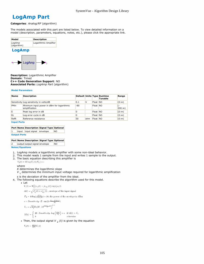
SystemVue - Algorithm Design Library
105
LogAmp PartCategories: Analog/RF (algorithm)
The models associated with this part are listed below. To view detailed information on amodel (description, parameters, equations, notes, etc.), please click the appropriate link.
Model Description
LogAmp(algorithm)
Logarithmic Amplifier
LogAmp
Description: Logarithmic AmplifierDomain: TimedC++ Code Generation Support: NOAssociated Parts: LogAmp Part (algorithm)
Model Parameters
Name Description Default Units Type RuntimeTunable
Range
Sensitivity Log sensitivity in volts/dB 0.1 V Float NO (0:∞)
PMin Minimum input power in dBm for logarithmicamplification
-80 Float NO (-200:∞)
E Peak log error in dB 0 Float NO [0:∞)
Ec Log error cycle in dB 0 Float NO (0:∞)
RefR Reference resistance 50 ohm Float NO (0:∞)
Input Ports
Port Name Description Signal Type Optional
1 input input signal envelope NO
Output Ports
Port Name Description Signal Type Optional
2 output output signal envelope NO
Notes/Equations
LogAmp models a logarithmic amplifier with some non-ideal behavior.1.This model reads 1 sample from the input and writes 1 sample to the output.2.The basic equation describing this amplifier is3.
whereK determines the logarithmic slopeV L determines the minimum input voltage required for logarithmic amplification
ε is the deviation of the amplifier from the ideal.The following equations describe the algorithm used for this model.4.
Let
Then, the output signal V 2 (t) is given by the equation

SystemVue - Algorithm Design Library
106
LogVDet PartCategories: Analog/RF (algorithm)
The models associated with this part are listed below. To view detailed information on amodel (description, parameters, equations, notes, etc.), please click the appropriate link.
Model Description
LogVDet(algorithm)
Logarithmic VideoDetector
LogVDet
Description: Logarithmic Video DetectorDomain: TimedC++ Code Generation Support: NOAssociated Parts: LogVDet Part (algorithm)
Model Parameters
Name Description Default Units Type RuntimeTunable
Range
Sensitivity Log sensitivity in volts/dB 0.1 V Float NO (0:∞)
PMin Minimum input power in dBm for logarithmicamplification
-80 Float NO (-200:∞)
E Peak log error in dB 0 Float NO [0:∞)
Ec Log error cycle in dB 0 Float NO (0:∞)
RefR Reference resistance 50 ohm Float NO (0:∞)
Input Ports
Port Name Description Signal Type Optional
1 input input signal envelope NO
Output Ports
Port Name Description Signal Type Optional
2 output output signal envelope NO
Notes/Equations
LogVDet models a logarithmic video detector with some non-ideal behavior.1.This model reads 1 sample from the input and writes 1 sample to the output.2.The basic equation describing this detector is:3.
whereK determines the logarithmic slopeVL determines the minimum input voltage required for logarithmic video detection
ε is the deviation of the detector from the ideal.The following equations describe the algorithm used for this model.4.
Let
Then, the output signal V2(t) is given by the equation
Example: S= 0.025v/dB, PMin = −80 dBm, E = 0.75 dB, EC = 10 dB

SystemVue - Algorithm Design Library
107

SystemVue - Algorithm Design Library
108
Mixer PartCategories: Analog/RF (algorithm)
The models associated with this part are listed below. To view detailed information on amodel (description, parameters, equations, notes, etc.), please click the appropriate link.
Model Description
Mixer(algorithm)
Envelope SignalMixer
Mixer (Signal Mixer)
Description: Envelope Signal MixerDomain: TimedC++ Code Generation Support: NOAssociated Parts: Mixer Part (algorithm)
Model Parameters
Name Description Default Units Type RuntimeTunable
Range
ConvGain Conversion gain in dB 0 Float NO (-∞:∞)
EnableNoise Enable mixer noise: NO, YES YES Enumeration NO
NoiseFigure Double sideband noise figure in dB 0 Float NO [0:∞)
Sideband Mixer primary output sideband:Lower, Upper
Lower Enumeration NO
SidebandSuppression Suppression of the outputalternate sideband in dB
-200 Float NO (-∞:0)
RfRej RF to outut rejection in dB -200 Float NO (-∞:0)
LoRej LO to output rejection in dB -200 Float NO (-∞:0)
LoRfIso LO to RF isolation in dB -200 Float NO (-∞:0)
RfLoIso RF to LO isolation in dB -200 Float NO (-∞:0)
SOIout Output second order interceptpower
1.0e17 W Float NO (0:∞)†
TOIout Output third order intercept power 1.0e17 W Float NO (0:∞)†
RefR Reference resistance 50 ohm Float NO (0:∞)
Input Ports
Port Name Description Signal Type Optional
1 input1 input signal1
envelope NO
2 input2 input signal2
envelope NO
Output Ports
Port Name Description Signal Type Optional
3 output output signal envelope NO
Notes/Equations
Mixer models an RF mixer for use with complex envelope input and local oscillator1.(LO) and includes many non-ideal mixer features such as noise figure, RF and LOleakage products, and 2 nd and 3 rd order nonlinearities.This block reads 1 sample from input1 and input2 and writes 1 sample to output.2.The Mixer primary signal of interest at the input1 is the RF signal with frequency f RF.3.
The RF signal mixes with the LO input at input2 with frequency f LO to produce the
lower sideband output signal with frequency |f LO - f RF| and the upper sideband
output signal with frequency (f LO + f RF). The mixer is operated with selection of
either the lower or upper output sideband as the primary sideband. The mixerconversion gain, ConvGain, is the ratio of the desired output sideband to the RF inputsignal level. The other sideband output level is controlled by theSidebandSuppression value.The Mixer block internal signal flow is diagramed.4.

SystemVue - Algorithm Design Library
109
Mixer operates with LO limiting and does not support any starved LO conditions,i.e. the LO always drives the mixer into saturation.Note that the linear gain precedes the nonlinear gain which precedes the mixingprocess.The mixing process is a 'linear' process performing frequency translation thatresults in lower and upper sideband products.vrf1 is the primary RF input signal at frequency f1 including any noise fromNoiseFigure.vrf2 is the secondary RF input signal leakage due to the LO at frequency f2appearing at the RF input.vlo1 is the primary LO input signal at frequency f2.vlo2 is the secondary LO input signal due to leakage from the RF input atfrequency f1 appearing at the LO input.
The Mixer input RF image frequency, f RFImage, is defined as the other input5.
frequency which results in a mixing product output at the specified output frequency.The input image is typically only of interest for receiver/down-conversion applicationsand is given by f RFImage = 2 * f LO - f RF.
The frequencies, f RF and f RFImage, both mix down with f LO to generate the output at
|f LO - f RF|. The signals f RF and f RFImage are called images of each other with
respect to the f LO.
In typical simulations, the f RFImage is often input noise that is located at a frequency
away from the desired f RF input modulated signal.
The Mixer output operating without nonlinearity can be defined with this expression:6.vout = vout A + vout B + vout2 A + vout2 B + vlo1 leak + vrf1 leak
wherevout A = mixer output due to mixing with the primary LO signal, vlo1, and at the
primary sideband based on the parameters Sideband and ConvGain.vout B = mixer output due to mixing with the primary LO signal, vlo1, and at the
alternate sideband based on the suppression parameter, SidebandSuppression,and ConvGain.vout2 A = mixer output due to mixing with the secondary LO signal, vlo2, at the
primary sideband based on the parameters Sideband and ConvGain.vout B = mixer output due to mixing with the secondary LO signal, vlo2, at the
alternate sideband based on the suppression parameter, SidebandSuppression,and ConvGain.vlo1 leak = mixer output due to leakage of the primary LO input signal appearing
at the output based on the rejection parameter, LoRej.vrf1 leak = mixer output due to leakage of the primary RF input signal appearing
at the output based on the rejection parameter, RfRej.The Mixer output operating with nonlinearity is defined by the SOIout and TOIout7.parameters.For definition of the SOI and TOI nonlinearities, see the detail discussion in thedocumentation for the AmplifierBB (algorithm) block.The nonlinearity is applied only to the RF path before the mixing process which iscomposed of vrf1 and vrf2.The Mixer self generated noise is added to the primary RF input signal, vrf1, and is8.defined by the parameters NoiseFigure and RefR .NoiseFigure for Mixer is defined as a double sideband noise figure, NFdsb, whichfollows industry conventions. The double sideband noise figure is converted to anequivalent single sideband noise figure, NFssb. That conversion is dependent onwhether the lower or the upper sideband is selected.
In general, the NFssb is related to the NFdsb as follows

SystemVue - Algorithm Design Library
110
NFssb = NFdsb + 10 * log( ( G1 + G2 +... ) / G1 )where
G1 is the primary power gain from the input noise frequency to the outputnoise frequencyG2 +... is the sum of all higher order mixing gains which is mixed fromsome input frequency to the output noise frequency.
For a mixer without input image rejection as is the case for this Mixer model, G2is significant and is often equal to G1 under small-signal operation while G3 +...is zero under small-signal conditions.Thus, the simplified expression, NFssb = NF + 10 * log( 1 + G2 / G1 ), is used.Note that the Mixer self noise is considered to be broadband such that it existsat all frequencies.Consider the case when Sideband is _Lower and choose f RF < f LO.
The primary lower output sideband is |f LO - f RF|. The input image for down-
conversion is at 2 * f LO - f RF. Its lower output sideband is due to mixing down
by the f LO which also gives |f LO - f RF|. The gain factor G2 is the same as G1
since both noise results from a frequency down conversion. Thus, the NFssb is 3dB more than the NFdsb, i.e. NFssb is NoiseFigure + 3.010299.Consider the case when Sideband is Upper and choose f RF < f LO.
The primary upper output sideband is |f LO + f RF|. The input image for up-
conversion is at 2 * f LO + f RF. Its lower output sideband is due to mixing down
by the f LO to also give |f LO + f RF|. At the same frequency, the first noise term
(G1) is due to an up conversion and the second noise term (G2) is due to adown conversion. Thus, the mixer gain for G2 will be different from the gain forG1 due to SidebandSuppression. The single sideband noise figure is increasedonly if the alternate sideband is not suppressed, i.e. NFssb = NoiseFigure + 10 *log( 1 + 10 ( SidebandSuppression / 10 ) ).
vn_rms, the rms noise voltage, is used to generate a complex Gaussian random9.value at each simulation time point which is then added to the input complexenvelope.Letk = Boltzmann constant is 1.380622e-23 J/Ksr = simulation sample rate of the block inputt0 = reference temperature in Kelvin is set at 290 Knf = 10 ( NFssb / 10)
thenHow does the simulation sample rate impact the Mixer model. Let the simulation10.sample rate be called sr and the primary mixer output frequency be called f out.
If Sideband is Upper, then f out is f LO + f RF.
Else Sideband is Lower, then f out is |f LO - f RF| provided there is ideal LO to RF
and RF to LO isolation, otherwise f out is set to 0 Hz.
There is ideal LO to RF isolation when LoRfIso is less then -200 dB. There isideal RF to LO isolation when RfLoIso is less then -200 dB.When there is non-ideal LO to RF or RF to LO isolation, f out is set to 0 Hz, since
the primary artifact of non-ideal LO to RF and RF to LO is frequency content ator near 0 Hz.For Mixer usage without suppression, leakage, isolation and nonlinearcharacteristics, the model is not dependent on the simulation sample rate. Itsimply mixes the RF input with the LO input to produce the selected sidebandoutput with mixer noise if specified.However, when the there are any suppression, leakage, isolation or nonlinearcharacteristics specified, then the simulation sample rate will impact how theseadditional effects are included in the mixer output signal.Each of these additional mixer characteristics may result in frequency terms thatreside outside the frequency range [f out - sr / 2, f out + sr / 2]. If frequency
terms are outside this range, they will be excluded from the output signal.In general, these frequency terms are excluded without warning. Warnings areissued when the sample rate is too small to support the effects of leakage termswhen LoRej > -200 dB or when SidebandSuppression > -200 dB.

SystemVue - Algorithm Design Library
111
MpyEnv PartCategories: Analog/RF (algorithm)
The models associated with this part are listed below. To view detailed information on amodel (description, parameters, equations, notes, etc.), please click the appropriate link.
Model Description
MpyEnv(algorithm)
Two Input Envelope Multiplier
MpyEnv
Description: Two Input Envelope MultiplierDomain: TimedC++ Code Generation Support: NOAssociated Parts: MpyEnv Part (algorithm)
Model Parameters
Name Description Default Units Type RuntimeTunable
SideBandType Multiplication product type: Lower sideband,Upper sideband, Both sidebands
Uppersideband
Enumeration NO
Input Ports
Port Name Description Signal Type Optional
1 input1 input signal1
envelope NO
2 input2 input signal2
envelope NO
Output Ports
Port Name Description Signal Type Optional
3 output output signal envelope NO
Notes/Equations
MpyEnv multiplies the two input complex envelope signals. It can be used to model1.an up-converter, down-converter, or double sideband modulator.This model reads 1 sample from all inputs and writes 1 sample to the output.2.The signals at pin k, where k is 1, 2, or 3, have complex envelope representation:3.
For SidebandType = Both4.When both inputs are complex envelope: v 3(t) = 0.5 v 1(k) conj(v 2(t)) + 0.5
conj(v 1(t)) v 2(t); f 3 = max(f 1, f 2)
When both inputs are real: v 3(t) = v 1(t) v 2(t); f 3 = 0
When one input is real: v 3(t) = v 1(t) v 2(t); f 3 = max(f 1, f 2)
For SidebandType = Upper sideband5.When either input is real: SidebandType is forced to Both and the output is setfor that case.When both inputs are complex envelope: v 3(t) = 0.5 v 1(t) v 2(t); f 3 = f 1 + f 2
For SidebandType = Lower sideband6.When either input is real: SidebandType is forced to Both and the output is setfor that case.When both inputs are complex envelope and f 1 > f 2 : v 3(t) = 0.5 v 1(t) conj(v 2(t)); f 3 = f 1 - f 2When both inputs are complex envelope and f 2 > f 1 : v 3(t) = 0.5 conj(v 1(t))
v 2(t); f 3 = f 2 - f 1When both inputs are complex envelope and f 1 = f 2 : v 3(t) = 0.5 v 1(t) conj(v 2(t)); f 3 = 0 and the imaginary part of v 3(t) is set to 0.0.
In the above, the function conj() takes the conjugate of the complex argument.7.
See:AddEnv (algorithm)SubEnv (algorithm)

SystemVue - Algorithm Design Library
112
MpyMultiEnv (algorithm)

SystemVue - Algorithm Design Library
113
NoiseFMask PartCategories: Analog/RF (algorithm), Sources (algorithm)
The models associated with this part are listed below. To view detailed information on amodel (description, parameters, equations, notes, etc.), please click the appropriate link.
Model Description
NoiseFMask(algorithm)
Noise Generator with Frequency Domain Mask Specification
NoiseFMask
Description: Noise Generator with Frequency Domain Mask SpecificationDomain: TimedC++ Code Generation Support: NOAssociated Parts: NoiseFMask Part (algorithm)
Model Parameters
Name Description Default Units Type RuntimeTunable
Range Symbol
FCarrierOption Signal carrierfrequency option:Carrier at center ofNoiseMask data,Defined by FCarrier
Carrier atcenter ofNoiseMaskdata
Enumeration NO
FCarrier Carrier frequency forthe noise (used ifFCarrierOption isDefined by FCarrier)
1000000 Hz Float NO (0:∞)
NoiseMask Noise specificationdefined with pairs ofvalues for frequency(Hz), noise level(dBm/Hz)
Floatingpoint array
NO
ResBW Resolution frequencybandwidth for noisespectrum
1e6 Hz Float NO (0:∞)†
RefR Reference resistance 50 ohm Float NO (0:∞)
ShowAdvancedParams Show advancedparameters: NO, YES
NO Enumeration NO
SampleRateOption Sample rate option:UnTimed, Timed fromSampleRate, Timedfrom Schematic
Timed fromSchematic
Enumeration NO SO
SampleRate Explicit sample rate Sample_Rate Hz Float NO (0:∞) S
InitialDelay Initial output timedelay
0 s Float YES [0:∞) D
Output Ports
Port Name Description Signal Type Optional
1 output output signal envelope NO
Notes/Equations
NoiseFMask generates an RF (complex envelope) noise signal with a power spectral1.density that follows the frequency domain noise mask as defined by NoiseMask.The NoiseMask parameter is an array of values that defines the mask. The values are2.interpreted as pairs of frequency in Hz and noise power level in dBm/Hz.The FCarrierOption and FCarrier parameters define the characterization frequency3.(fc) of the output signal.
For FCarrierOption set to Carrier at center of NoiseMask data, fc is the averageof the effective smallest and largest frequencies listed in NoiseMask.For FCarrierOption set to Defined by FCarrier, fc is FCarrier.
The output signal is modeled as a sum of tones.4.Number of tones is (fmax - fmin) / ResBW. Let SR be the simulation sample rate
for this model instance. If fmin is less than fc - (SR / 2), then it is reset to this
limit. If fmax is greater than fc + (SR / 2), then it is reset to this limit. More
tones allow for more accurate modeling in the output noise. However, usingmore tones will increase simulation time.Frequency of the ith tone is selected from a uniform distribution in the interval [f
+ i·ResBW, f + (i + 1)·ResBw).

SystemVue - Algorithm Design Library
114
min min
Amplitude of the ith tone is selected from a normal distribution centered aroundan amplitude that corresponds to the power level specified in the mask. Powerlevels for tones whose frequency is not listed in the NoiseMask parameter areinterpolated. The power level is converted to voltage level using the referenceresistance, RefR.Initial phase of each tone is selected from a uniform distribution in the interval[0, 2·π).
For other parameter descriptions, see Timed Sources (algorithm).5.

SystemVue - Algorithm Design Library
115
Oscillator PartCategories: Analog/RF (algorithm), Sources (algorithm)
The models associated with this part are listed below. To view detailed information on amodel (description, parameters, equations, notes, etc.), please click the appropriate link.
Model Description
Oscillator(algorithm)
Oscillator with Carrier Frequency
Oscillator
Description: Oscillator with Carrier FrequencyDomain: TimedC++ Code Generation Support: NOAssociated Parts: Oscillator Part (algorithm)
Model Parameters
Name Description Default Units Type RuntimeTunable
Range Symbol
Frequency RF tone frequency 1000000 Hz Float NO (0:∞)
Power RF tone carrier power .010 W Float NO [0:∞)
Phase RF tone carrier phase 0.0 deg Float NO (-∞:∞)
RandomPhase Set phase of RF tone torandom value between-PI and +PI: NO, YES
NO Enumeration NO
PhaseNoiseData Phase noisespecification - pairs ofoffset freq (Hz) andSSB phase noise level(dBc/Hz)
Floatingpoint array
NO
PN_Type Phase noise modeltype with random orfixed offset freqspacing and amplitude:Random PN, Fixed freqoffset, Fixed freq offsetand amplitude
Random PN Enumeration NO
NDensity Noise spectral densityadded
0 W Float NO [0:∞)
RefR Reference resistance 50 ohm Float NO (0:∞)
ShowAdvancedParams Show advancedparameters: NO, YES
NO Enumeration NO
SampleRateOption Sample rate option:UnTimed, Timed fromSampleRate, Timedfrom Schematic
Timed fromSchematic
Enumeration NO SO
SampleRate Explicit sample rate Sample_Rate Hz Float NO (0:∞) S
InitialDelay Initial output timedelay
0 s Float YES [0:∞) D
Output Ports
Port Name Description Signal Type Optional
1 output output signal envelope NO
Notes/Equations
Oscillator generates an RF (complex envelope) defined by its carrier frequency and1.with optional thermal noise and phase noise.The frequency, power, and phase of the first tone are defined by the Frequency,2.Power and Phase parameters, respectively.If RandomPhase=Yes, then the Phase is ignored and a random phase between −1803.and +180 degrees is used.Noise power added to the output signal is NDensity_W × BW where4.NDensity_W is the noise density in Watts/Hz. The NDensity parameter specified inany power unit automatically converts to NDensity_W.BW is the simulation bandwidth which, for complex envelope signal, is the samplerate.The rms voltage associated with the noise power is .The value of NDensity (in Watts/Hz) is related to temperature in Kelvin as kT where k

SystemVue - Algorithm Design Library
116
is the Boltzmann constant (1.3806504e-23). At the standard system temperature of290 Kelvin (16.85 Celsius), the NDensity is 4.00388587e-21 Watts/Hz (-173.975dBm/Hz).A phase noise characteristic is specified in the PhaseNoiseData list. This list contains5.double values of offset frequency (Hz) and single sideband relative power level(dBc/Hz).
PhaseNoiseData = "[100, -50, 1000, -70, 1e5, -90]" or alternatively can reference an array
defined using Math Language in an Equations sheet.
The phase noise characteristic defined from this list describes a frequency domainspecification for phase noise. Interpolation is applied between these frequencydomain points as needed to give a full time domain simulation definition for thisphase noise.
Phase noise is modeled as a sum of tones that modulates the phase of the main tone. Let f
offsetMax (foffsetMin) be the maximum (minimum) offset frequency specified in
PhaseNoiseData. Then the number of tones N used to model phase noise is equal to f
offsetMax / foffsetMin.
In the following, let ROut = RefR, the power specification reference resistance.Let Pi be the phase noise power at frequency offset fi. The phase (φi), frequency (fi), and
amplitude (or modulation index) (ηi) of each tone is given by:
When PN_Type = Fixed freq offset and amplitude
φi is a random variable uniformly distributed in [0, 2π)
fi = i·foffsetMin
ηi =
When PN_Type = Fixed freq offset
φi is a random variable uniformly distributed in [0, 2π)
fi = i·foffsetMin
ηi is a random variable with a Rayleigh distribution with parameter σ =
When PN_Type = Random PN
φi is a random variable uniformly distributed in [0, 2π)
fi is a random variable uniformly distributed in [(i-0.5)·foffsetMin, (i+0.5)·foffsetMin]
ηi =
For the first two cases Fixed freq offset and amplitude and Fixed freq offset, phase noise isa sum of tones whose frequencies are integer multiples of the same frequency (foffsetMin).
Therefore, phase noise will be periodic with period 1 / foffsetMin and all the phase noise
signal power will be located at the discrete frequencies that are integer multiples of f
offsetMin. When a spectrum analysis is performed on this signal and the resolution
bandwidth is equal to foffsetMin / M, where M is an integer, the spectrum will have spectral
nulls (e.g. -250 dBm) at all frequencies that are not an integer multiple of foffsetMin . The
integrated power in a bandwidth of foffsetMin will still be what one expects based on the
phase noise data specification but it will all be concentrated at one frequency (the one thatis an integer multiple of foffsetMin).
For better phase noise modeling it is recommended that simulations be performed withPN_Type set to Random PN (default). The other values for PN_Type can be used todemonstrate/understand the phase noise modeling algorithm and are not recommendedfor use in practical simulations.The single sideband phase noise in dBc/Hz is
whereη (f ) = root mean square of modulation index η at offset frequency f .

SystemVue - Algorithm Design Library
117
rms i i i
The modulation index is related to the signal power and single sideband phase noisepower as follows:
wherePc = signal power
Pssb (fi ) = signal sideband power at offset frequency fiTherefore, single sideband phase noise in dBc/Hz can also be expressed as:
wherePssb (fi)dBm = simulated single sideband phase noise power per simulation frequency
resolution bandwidth ResBWResBWdB = factor for frequency resolution bandwidth ResBW used during simulation = 10× log10(ResBW)Pc dBm = signal power in dBm
NoteIf the phase noise settings result in the summed phase noise higher than tone power (dBm) - 10 dB, awarning message will be generated:Phase noise violates small signal modeling requirement; phase noise power exceeds Tone_Power (dBm) -10 dB.However, the simulation will continue with the current parameter settings.
A phase noise modeling example is demonstrated here. Consider the simple design withan Oscillator used to generate a 1 GHz tone at a power level of 10 dBm with 50 Ohmsreference resistance. The tone is colored with phase noise, whose frequency specificationis defined with PhaseNoiseData = 1.0e3, -70, 1.0e4, -60, 4.0e4, -60, 4.0e5, -90. For thisexample, foffsetMin is 1 kHz and foffsetMax is 400 kHz. The simulation sample rate
(Sample_Rate) is set to (8192 / Stop_Time ) Hz, which is large enough to resolve themaximum phase noise frequency offset data point at 400 kHz. The simulation stop time(Stop_Time) is set to 1 msec, which is large enough to resolve the lowest phase noisefrequency offset data point at 1 kHz.The spectrum of the signal at the output of N_Tones is measured using aSpectrumAnalyzer component. The spectrum is shown in Signal Spectrum withPN_Type=Random PN and TStop=1 msec. The resolution bandwidth of the spectrummeasurement is 1 / ( Stop - Start ) = 1 / ( 1 msec ) = 1 kHz. This means that eachspectral tone displayed will be at multiples of 1 kHz from the carrier frequency of 1 GHz.For noise power integrated over a 1 kHz bandwidth, the power would be 30 dB(=10 × log10(1000)) more than that in a 1 Hz bandwidth.
Signal Spectrum with PN_Type= Random PN and TStop=1 msec
Signal Spectrum with PN_Type=Fixed freq offset and amplitude and TStop=2 msec showsthe signal spectrum when PN_Type= Fixed freq offset and amplitude and TStop=2 msec.The resolution bandwidth of the spectrum measurement is 1 / ( Stop - Start ) = 0.5 kHz.As explained in note 6, all phase noise signal power will be located at frequencies that areinteger multiples of foffsetMin = 1 kHz and the spectrum values at frequencies (M+0.5) kHz
(where M is an integer) will be practically 0.
Signal Spectrum with PN_Type= Fixed freq offset and amplitude and TStop=2 msec

SystemVue - Algorithm Design Library
118
To view the phase noise spectrum versus spectral tone offset index, a signal processingnetwork can be created to perform the FFT on the collected RF complex time domainwaveform. Summed powers in the upper and lower sidebands are averaged and resultsare converted into dBm to obtain the single sideband phase noise power in dBm persimulation frequency resolution bandwidth versus offset spectral tone. This resultantsingle sideband phase noise spectrum can be displayed versus spectral tone offset indexas shown in Phase Noise Spectrum with PN_Type=Random PN. In Phase Noise Spectrum with PN_Type=Random PN, 1 kHz offset occurs at index 1, 10kHz offset occurs at index 10, 40 kHz offset occurs at index 40, and 400 kHz offset occursat index 400. As can be seen, this figure agrees with the PhaseNoiseData specified.The phase noise data displayed in Phase Noise Spectrum with PN_Type=Random PN wasgenerated using PN_Type= Random PN . In Phase Noise Spectrum with PN_Type=Fixedfreq offset and amplitude, phase noise is displayed with PN_Type= Fixed freq offset andamplitude . As can be seen, Phase Noise Spectrum with PN_Type=Fixed freq offset andamplitude agrees much better (compared to Phase Noise Spectrum withPN_Type=Random PN) with the PhaseNoiseData specified, since in this case there is norandomness in the values of fi and ηi.
The results of Phase Noise Spectrum with PN_Type=Random PN and Phase NoiseSpectrum with PN_Type=Fixed freq offset and amplitude were obtained by setting the FFTsize to 2 13.
Phase Noise Spectrum with PN_Type= Random PN
Phase Noise Spectrum with PN_Type= Fixed freq offset and amplitude
For other parameter descriptions, see Time Burst Sources.
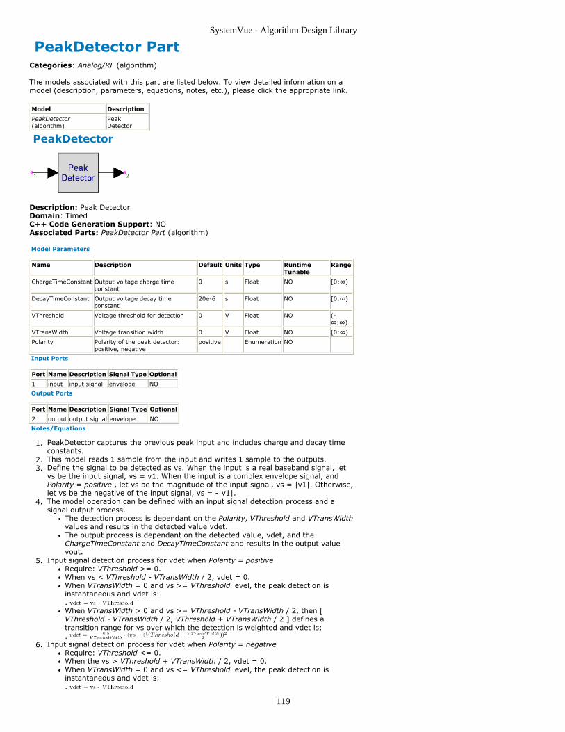
SystemVue - Algorithm Design Library
119
PeakDetector PartCategories: Analog/RF (algorithm)
The models associated with this part are listed below. To view detailed information on amodel (description, parameters, equations, notes, etc.), please click the appropriate link.
Model Description
PeakDetector(algorithm)
PeakDetector
PeakDetector
Description: Peak DetectorDomain: TimedC++ Code Generation Support: NOAssociated Parts: PeakDetector Part (algorithm)
Model Parameters
Name Description Default Units Type RuntimeTunable
Range
ChargeTimeConstant Output voltage charge timeconstant
0 s Float NO [0:∞)
DecayTimeConstant Output voltage decay timeconstant
20e-6 s Float NO [0:∞)
VThreshold Voltage threshold for detection 0 V Float NO (-∞:∞)
VTransWidth Voltage transition width 0 V Float NO [0:∞)
Polarity Polarity of the peak detector:positive, negative
positive Enumeration NO
Input Ports
Port Name Description Signal Type Optional
1 input input signal envelope NO
Output Ports
Port Name Description Signal Type Optional
2 output output signal envelope NO
Notes/Equations
PeakDetector captures the previous peak input and includes charge and decay time1.constants.This model reads 1 sample from the input and writes 1 sample to the outputs.2.Define the signal to be detected as vs. When the input is a real baseband signal, let3.vs be the input signal, vs = v1. When the input is a complex envelope signal, andPolarity = positive , let vs be the magnitude of the input signal, vs = |v1|. Otherwise,let vs be the negative of the input signal, vs = -|v1|.The model operation can be defined with an input signal detection process and a4.signal output process.
The detection process is dependant on the Polarity, VThreshold and VTransWidthvalues and results in the detected value vdet.The output process is dependant on the detected value, vdet, and theChargeTimeConstant and DecayTimeConstant and results in the output valuevout.
Input signal detection process for vdet when Polarity = positive5.Require: VThreshold >= 0.When vs < VThreshold - VTransWidth / 2, vdet = 0.When VTransWidth = 0 and vs >= VThreshold level, the peak detection isinstantaneous and vdet is:. When VTransWidth > 0 and vs >= VThreshold - VTransWidth / 2, then [VThreshold - VTransWidth / 2, VThreshold + VTransWidth / 2 ] defines atransition range for vs over which the detection is weighted and vdet is:.
Input signal detection process for vdet when Polarity = negative6.Require: VThreshold <= 0.When the vs > VThreshold + VTransWidth / 2, vdet = 0.When VTransWidth = 0 and vs <= VThreshold level, the peak detection isinstantaneous and vdet is:.
SystemVue - Algorithm Design Library
120
When VTransWidth > 0 and vs <= VThreshold + VTransWidth / 2, then [VThreshold - VTransWidth / 2, VThreshold + VTransWidth / 2 ] defines atransition range for vs over which the detection is weighted and vdet is:.
Signal output process for vout7.When the new value for vdet is greater then the prior value for vout, then thenew vout value will charge to this new vdet value dependant on theChargeTimeConstant.
When ChargeTimeConstant = 0 and vdet > vout, then the charge isinstantenous and vout = vdet.When ChargeTimeConstant > = 0, then a test is performed to determine ifvout should continue to charge.. Where, SR = the simulation sample rate for the model instance.If vtest > vout, then vout is reset to vtest.
When the new value for vdet is less then the prior value for vout, then the newvout value will decay to this new vdet value dependant on theDelayTimeConstant.
When DecayTimeConstant = 0 and vdet < vout, then the decay isinstantaneous and vout = vdet.When DecayTimeConstant is large, then vout is held indefintely untilchanged by a new vdet value.When DecayTimeConstant > = 0, then a test is performed to determine ifvout should continue to decay.. Where, SR = the simulation sample rate for the model instance.If vtest < vout, then vout is reset to vtest.

SystemVue - Algorithm Design Library
121
PhaseComparator PartCategories: Analog/RF (algorithm)
The models associated with this part are listed below. To view detailed information on amodel (description, parameters, equations, notes, etc.), please click the appropriate link.
Model Description
PhaseComparator(algorithm)
Phase Comparator
PhaseComparator
Description: Phase ComparatorDomain: TimedC++ Code Generation Support: NOAssociated Parts: PhaseComparator Part (algorithm)
Model Parameters
Name Description Default Units Type RuntimeTunable
Range
PhaseCharacteristicType Type of analog phasecomparator: PhaseFreq,Sinusoidal, Triangular
PhaseFreq Enumeration NO
GainConstant Small signal gain constant, involts per degree
1 Float NO (-∞:0)or(0:∞)
MaxAngle Maximum unwrapped phaseangle (+/- MaxAngle) forPhaseCharacteristicType =PhaseFreq
360 Float NO
Input Ports
Port Name Description Signal Type Optional
1 s1 input signal1
envelope NO
2 s2 input signal2
envelope NO
Output Ports
Port Name Description Signal Type Optional
3 output output signal envelope NO
Notes/Equations
PhaseCompRF models a phase comparator which compare two complex envelope1.signals. The output can be a linear difference or a difference that has sine ortriangular characteristics. This model reads 1 sample from the inputs and writes 1 sample to the output.2.This model is useful in the design of RF phase lock loops.3.This model requires that both inputs are complex envelope signals with4.characterization frequencies (fc1, fc2) greater than zero. Real input signals are notallowed by this model. If use with a real is needed, then the input to this model canbe preceeded with an EnvFcChange (algorithm) model that will recharacterize a realsignal to its representation at a specified frequency. The simulation rate for thismodel must be large enough to enable both input signals to be represented at thesame characterization frequency as s1. Otherwise, a warning message will bedisplayed. In the following, the phase angles for s1 and s2 are discussed after s2 isconverted to its characterization at fc1 (if fc2 is not the same as fc1).The output is calculated as follows:5.θ 1 (t) denotes the phase angle associated with s1.
θ 2 (t) denotes the phase angle associated with s2.
K is the GainConstant parameter value.The output signal at pin 3 is
. diff(t) is the difference between the unwrapped phase between s1 and s2 withmodulo MaxAngle.The triangular() function is shown below.

SystemVue - Algorithm Design Library
122
Phase Comparator Characteristics
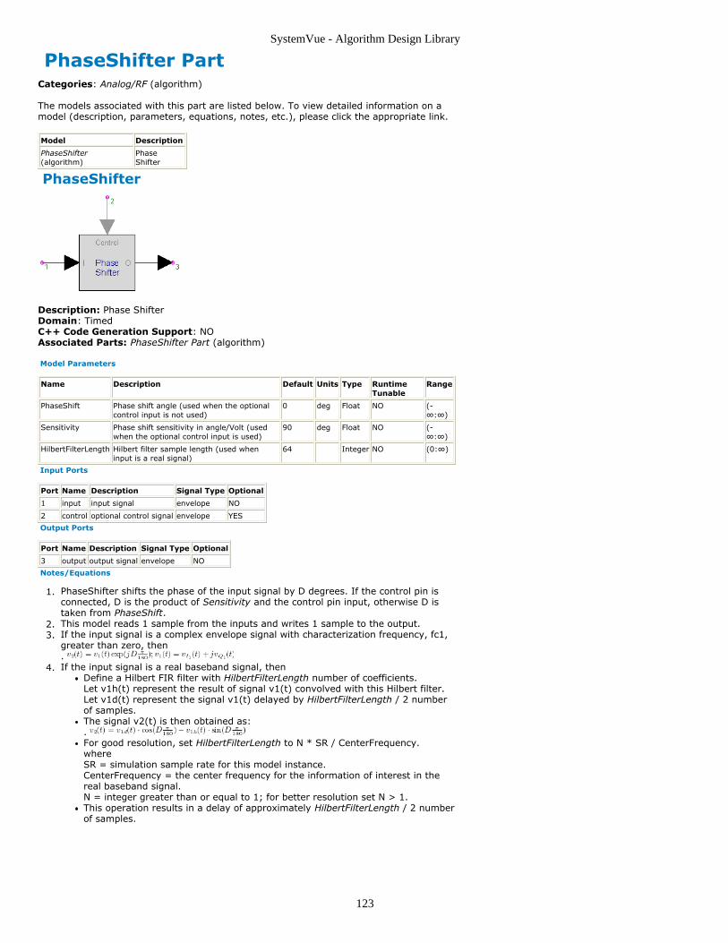
SystemVue - Algorithm Design Library
123
PhaseShifter PartCategories: Analog/RF (algorithm)
The models associated with this part are listed below. To view detailed information on amodel (description, parameters, equations, notes, etc.), please click the appropriate link.
Model Description
PhaseShifter(algorithm)
PhaseShifter
PhaseShifter
Description: Phase ShifterDomain: TimedC++ Code Generation Support: NOAssociated Parts: PhaseShifter Part (algorithm)
Model Parameters
Name Description Default Units Type RuntimeTunable
Range
PhaseShift Phase shift angle (used when the optionalcontrol input is not used)
0 deg Float NO (-∞:∞)
Sensitivity Phase shift sensitivity in angle/Volt (usedwhen the optional control input is used)
90 deg Float NO (-∞:∞)
HilbertFilterLength Hilbert filter sample length (used wheninput is a real signal)
64 Integer NO (0:∞)
Input Ports
Port Name Description Signal Type Optional
1 input input signal envelope NO
2 control optional control signal envelope YES
Output Ports
Port Name Description Signal Type Optional
3 output output signal envelope NO
Notes/Equations
PhaseShifter shifts the phase of the input signal by D degrees. If the control pin is1.connected, D is the product of Sensitivity and the control pin input, otherwise D istaken from PhaseShift.This model reads 1 sample from the inputs and writes 1 sample to the output.2.If the input signal is a complex envelope signal with characterization frequency, fc1,3.greater than zero, then. If the input signal is a real baseband signal, then4.
Define a Hilbert FIR filter with HilbertFilterLength number of coefficients.Let v1h(t) represent the result of signal v1(t) convolved with this Hilbert filter.Let v1d(t) represent the signal v1(t) delayed by HilbertFilterLength / 2 numberof samples.The signal v2(t) is then obtained as:. For good resolution, set HilbertFilterLength to N * SR / CenterFrequency.whereSR = simulation sample rate for this model instance.CenterFrequency = the center frequency for the information of interest in thereal baseband signal.N = integer greater than or equal to 1; for better resolution set N > 1.This operation results in a delay of approximately HilbertFilterLength / 2 numberof samples.
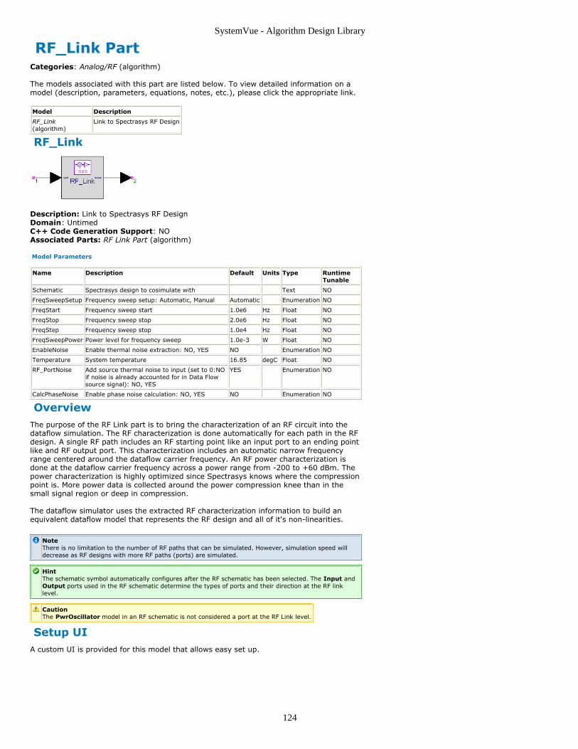
SystemVue - Algorithm Design Library
124
RF_Link PartCategories: Analog/RF (algorithm)
The models associated with this part are listed below. To view detailed information on amodel (description, parameters, equations, notes, etc.), please click the appropriate link.
Model Description
RF_Link(algorithm)
Link to Spectrasys RF Design
RF_Link
Description: Link to Spectrasys RF DesignDomain: UntimedC++ Code Generation Support: NOAssociated Parts: RF Link Part (algorithm)
Model Parameters
Name Description Default Units Type RuntimeTunable
Schematic Spectrasys design to cosimulate with Text NO
FreqSweepSetup Frequency sweep setup: Automatic, Manual Automatic Enumeration NO
FreqStart Frequency sweep start 1.0e6 Hz Float NO
FreqStop Frequency sweep stop 2.0e6 Hz Float NO
FreqStep Frequency sweep stop 1.0e4 Hz Float NO
FreqSweepPower Power level for frequency sweep 1.0e-3 W Float NO
EnableNoise Enable thermal noise extraction: NO, YES NO Enumeration NO
Temperature System temperature 16.85 degC Float NO
RF_PortNoise Add source thermal noise to input (set to 0:NOif noise is already accounted for in Data Flowsource signal): NO, YES
YES Enumeration NO
CalcPhaseNoise Enable phase noise calculation: NO, YES NO Enumeration NO
OverviewThe purpose of the RF Link part is to bring the characterization of an RF circuit into thedataflow simulation. The RF characterization is done automatically for each path in the RFdesign. A single RF path includes an RF starting point like an input port to an ending pointlike and RF output port. This characterization includes an automatic narrow frequencyrange centered around the dataflow carrier frequency. An RF power characterization isdone at the dataflow carrier frequency across a power range from -200 to +60 dBm. Thepower characterization is highly optimized since Spectrasys knows where the compressionpoint is. More power data is collected around the power compression knee than in thesmall signal region or deep in compression.
The dataflow simulator uses the extracted RF characterization information to build anequivalent dataflow model that represents the RF design and all of it's non-linearities.
NoteThere is no limitation to the number of RF paths that can be simulated. However, simulation speed willdecrease as RF designs with more RF paths (ports) are simulated.
HintThe schematic symbol automatically configures after the RF schematic has been selected. The Input andOutput ports used in the RF schematic determine the types of ports and their direction at the RF linklevel.
CautionThe PwrOscillator model in an RF schematic is not considered a port at the RF Link level.
Setup UIA custom UI is provided for this model that allows easy set up.
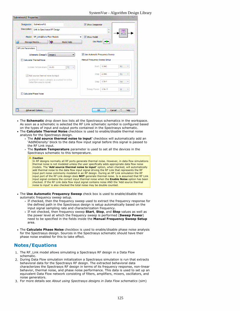
SystemVue - Algorithm Design Library
125
The Schematic drop down box lists all the Spectrasys schematics in the workspace.As soon as a schematic is selected the RF Link schematic symbol is configured basedon the types of input and output ports contained in the Spectrasys schematic.The Calculate Thermal Noise checkbox is used to enable/disable thermal noiseanalysis for the Spectrasys design.
The Add source thermal noise to input' checkbox will automatically add an'AddNDensity' block to the data flow input signal before this signal is passed tothe RF Link input.The System Temperature parameter is used to set all the devices in theSpectrasys schematic to this temperature.
CautionIn RF designs normally all RF ports generate thermal noise. However, in data flow simulationsthermal noise is not modeled unless the user specifically adds appropriate data flow noisemodels. The 'Add source thermal noise to input' option, when checked, will automaticallyadd thermal noise to the data flow input signal driving the RF Link that represents the RFinput port noise commonly modeled in an RF design. During an RF Link simulation the RFinput port of the RF Link design does NOT generate thermal noise. Is is assumed that RF Linkinput signal contains the correct input thermal noise when the Enable Noise option has beenchecked. If the RF Link data flow input signal contains noise AND the 'Add source thermalnoise to input' is also checked the total noise may be double counted.
The Use Automatic Frequency Sweep check box is used to enable/disable theautomatic frequency sweep setup.
If checked, then the frequency sweep used to extract the frequency response forthe defined path in the Spectrasys design is setup automatically based on theinput signal sampling rate and characterization frequency.If not checked, then frequency sweep Start, Stop, and Step values as well asthe power level at which the frequency sweep is performed (Sweep Power)need to be specified in the fields inside the Manual Frequency Sweep Setuparea.
The Calculate Phase Noise checkbox is used to enable/disable phase noise analysisfor the Spectrasys design. Sources in the Spectrasys schematic should have theirphase noise enabled for this to take effect.
Notes/EquationsThe RF_Link model allows simulating a Spectrasys RF design in a Data Flow1.schematic.During Data Flow simulation initialization a Spectrasys simulation is run that extracts2.behavioral data for the Spectrasys RF design. The extracted behavioral datacharacterizes the Spectrasys RF design in terms of its frequency response, non-linearbehavior, thermal noise, and phase noise performance. This data is used to set up anequivalent Data Flow network consisting of filters, amplifiers, mixers, oscillators, andnoise generators.For more details see About using Spectrasys designs in Data Flow schematics (sim)3.

SystemVue - Algorithm Design Library
126
SwitchSPDT PartCategories: Analog/RF (algorithm)
The models associated with this part are listed below. To view detailed information on amodel (description, parameters, equations, notes, etc.), please click the appropriate link.
Model Description
SwitchSPDT(algorithm)
Single Pole Double Throw Switch
SwitchSPDT
Description: Single Pole Double Throw SwitchDomain: TimedC++ Code Generation Support: NOAssociated Parts: SwitchSPDT Part (algorithm)
Model Parameters
Name Description Default Units Type RuntimeTunable
Range
Loss1 Loss in dB for on state insertion loss for output1
0 Float NO [0:+200)
Isolation1 Isolation in dB for off state insertion loss foroutput 1
200 Float NO [0:+200)
Loss2 Loss in dB for on state insertion loss for output2
0 Float NO [0:+200)
Isolation2 Isolation in dB for off state insertion loss foroutput 2
200 Float NO [0:+200)
VThreshold Control voltage threshold 0.5 V Float NO (0:∞)
TOn1 On state transition time for output 1 0 s Float NO [0:∞)
TOff1 Off state transition time for output 1 0 s Float NO [0:∞)
TOn2 On state transition time for output 2 0 s Float NO [0:∞)
TOff2 Off state transition time for output 2 0 s Float NO [0:∞)
Input Ports
Port Name Description Signal Type Optional
1 input1 input signal1
envelope NO
2 input2 input signal2
envelope NO
Output Ports
Port Name Description Signal Type Optional
3 output1 output signal 1 envelope NO
4 output2 output signal 2 envelope NO
Notes/Equations
SwitchSPDT models a single pole double throw switch with non-idealities including1.insertion loss, imperfect isolation, and non-zero switching time.This model reads 1 sample from the inputs and writes 1 sample to the outputs.2.The outputs take on the attributes of input1. If input1 is a real baseband signal, the3.the outputs will be. If the input1 is a complex envelope signal, then the output willalso be with the same characterization frequency. The input2 is always interpreted asa real baseband signal. If input2 is a complex envelope signal, it will be convertedinternally in this model to its equivalent form as a real baseband signal.SwitchSPDT inputs and output are defined as follows.4.Let v i(t) be the real or complex envelop value at pin i.
The control input v 2(t) is always forced to a real value for comparison with
VThreshold.Case 1: v 2(t) > VThreshold connects pin 1 to pin 4.
Let T s be the time at which v 2(t) exceeds VThreshold. Then

SystemVue - Algorithm Design Library
127
Case 2: v 2(t) ≤ VThreshold connects pin 1 to pin 3.
Let T s be the time at which v 2(t) falls below VThreshold. Then
A SwitchSPDT Example
The SwitchSPDT example uses a 1 KHz cosine input at pin 1 and a 0.5 KHz square1.wave control at pin 2.
An ideal SwitchSPDT part with the following parameters give the following output.2.Loss1=0 dB, Isolation1=200 dB,Loss2=0 dB, Isolation2=200 dB,VThreshold=0.50,TOn1=0 s, TOff1=0 s,TOn2=0 s, TOff2=0 s
A non-ideal SwitchSPDT part with the following parameters give the following output.3.Loss1=3 dB, Isolation1=20 dB,Loss2=3 dB, Isolation2=20 dB,VThreshold=0.50,TOn1=0.15 s, TOff1=0.15 s,TOn2=0.15 s, TOff2=0.15 s

SystemVue - Algorithm Design Library
128

SystemVue - Algorithm Design Library
129
SwitchSPST PartCategories: Analog/RF (algorithm)
The models associated with this part are listed below. To view detailed information on amodel (description, parameters, equations, notes, etc.), please click the appropriate link.
Model Description
SwitchSPST(algorithm)
Single Pole Single ThrowSwitch
SwitchSPST
Description: Single Pole Single Throw SwitchDomain: TimedC++ Code Generation Support: NOAssociated Parts: SwitchSPST Part (algorithm)
Model Parameters
Name Description Default Units Type Runtime Tunable Range
Loss Loss in dB for on state insertion loss 0 Float NO [0:+200)
Isolation Isolation in dB for off state insertion loss -200 Float NO [0:+200)
VThreshold Control voltage threshold 0.5 V Float NO (0:∞)
TOn On-state transition ctime for output 0 s Float NO [0:∞)
TOff Off-state transition ctime for output 0 s Float NO [0:∞)
Input Ports
Port Name Description Signal Type Optional
1 input1 input signal1
envelope NO
2 input2 input signal2
envelope NO
Output Ports
Port Name Description Signal Type Optional
3 output output signal envelope NO
Notes/Equations
SwitchSPST models a single pole single throw switch with non-idealities including1.insertion loss, imperfect isolation, and non-zero switching time.This model reads 1 sample from the inputs and writes 1 sample to the output.2.The output take on the attributes of input1. If input1 is a real baseband signal, the3.the output will be. If the input1 is a complex envelope signal, then the output willalso be with the same characterization frequency. The input2 is always interpreted asa real baseband signal. If input2 is a complex envelope signal, it will be convertedinternally in this model to its equivalent form as a real baseband signal.SwitchSPST inputs and output are defined as follows4.Let v i(t) be the real or complex envelop value at pin i.The control input v 2(t) is always forced to a real value for comparison withVThreshold.Case 1: v 2 (t) > VThreshold
Let T s be the time at which v 2 (t) exceeds VThreshold.
Then
Case 2: v 2 (t) ≤ VThreshold
Let T s be the time at which v 2 (t) falls below VThreshold.

SystemVue - Algorithm Design Library
130
Then
SwitchSPST Component Inputs and SwitchSPST Component Output show the5.performance of the SwitchSPST component, when it is an ideal switch, using thefollowing parameter values:Loss=0, Iso=200, Vth=0.50, Ton=0, Toff=0SwitchSPST Component Output shows the output of the SwitchSPST component,when the switch is not ideal, using the parameter values:Loss=3 dB, Iso=20 dB, Vth=0.50, Ton=0.15 s, Toff=0.15 s
SwitchSPST Component Inputs
SwitchSPST Component Output
SwitchSPST Component Output

SystemVue - Algorithm Design Library
131

SystemVue - Algorithm Design Library
132
TimeDelay PartCategories: Analog/RF (algorithm), Signal Processing (algorithm)
The models associated with this part are listed below. To view detailed information on amodel (description, parameters, equations, notes, etc.), please click the appropriate link.
Model Description
TimeDelay(algorithm)
Ideal Time Delay Block. Delays the signal for a certain amount oftime.
TimeDelay
Description: Ideal Time Delay Block. Delays the signal for a certain amount of time.Domain: TimedC++ Code Generation Support: NOAssociated Parts: TimeDelay Part (algorithm)
Model Parameters
Name Description Default Units Type Runtime Tunable Range
Unit Time delay unit: Time,TimeStep
Time Enumeration NO
T Delay in time 0 s Float NO [0, ∞)
N Delay in number of time steps 0 Integer NO [0, ∞)
Input Ports
Port Name Signal Type Optional
1 input anytype NO
Output Ports
Port Name Signal Type Optional
2 output anytype NO
Notes/Equations
TimeDelay delays the signal in time.1.For every input, one value is output.2.If Unit is Time, the input is delayed by T where T is any non-negative number.3.Otherwise, the input is delayed by N × time step where N is any non-negative4.integer.TimeDelay increases the time stamps by the delay without inserting zero valued5.samples.See page on Special Models in Timing Method (sim).6.

SystemVue - Algorithm Design Library
133
TimeSynchronizer PartCategories: Analog/RF (algorithm), Signal Processing (algorithm)
The models associated with this part are listed below. To view detailed information on amodel (description, parameters, equations, notes, etc.), please click the appropriate link.
Model Description
TimeSynchronizer(algorithm)
Synchronize signals intime
TimeSynchronizer
Description: Synchronize signals in timeDomain: TimedC++ Code Generation Support: NOAssociated Parts: TimeSynchronizer Part (algorithm)
Model Parameters
Name Description Default Units Type RuntimeTunable
Mode Time synchronization mode: ZeroPadding,TimeDelay
ZeroPadding Enumeration NO
Input Ports
Port Name Signal Type Optional
1 input multiple anytype NO
Output Ports
Port Name Signal Type Optional
2 output multiple anytype NO
Notes/Equations
TimeSynchronizer aligns multiple inputs in time.1.This model reads 1 sample from each of the inputs and writes 1 sample to each of2.the outputs.The _i_th input flows to _i_th output, therefore the number of the input connections3.must at least equal to the number of the output connections.If Mode is ZeroPadding, zero valued samples are inserted to later arriving inputs such4.that all signals are aligned in time to the earliest incoming signal.Otherwise, the earlier incoming signal time stamps are adjusted without inserting5.zeros such that all signals are aligned to the latest incoming signal.See section on Special Models in Timing Method (sim).6.

SystemVue - Algorithm Design Library
134
UpSampleEnv PartCategories: Analog/RF (algorithm), Routers/Resamplers (algorithm)
The models associated with this part are listed below. To view detailed information on amodel (description, parameters, equations, notes, etc.), please click the appropriate link.
Model Description
UpSampleEnv(algorithm)
Up Sampler for Envelope Signal
UpSampleEnv
Description: Up Sampler for Envelope SignalDomain: TimedC++ Code Generation Support: NOAssociated Parts: UpSampleEnv Part (algorithm)
Model Parameters
Name Description Default Units Type RuntimeTunable
Range
Factor Upsampling ratio 5 Integer NO [1:∞)
Mode Upsampling interpolation type: Insertzeros, Hold sample, Polyphase filter,Linear
Holdsample
Enumeration NO
Phase Upsampling insertion phase for the outputnon-zero sample
0 Integer NO [0:Factor -1]
ExcessBW Excess bandwidth of raised cosineinterpolation filter
0.5 Float NO [0:1]
Input Ports
Port Name Description Signal Type Optional
1 input input signal envelope NO
Output Ports
Port Name Description Signal Type Optional
2 output output signal envelope NO
To avoid confusion on a schematic, it is best to mirror (flip) this symbol (instead of rotating it) when youneed to have the input on the right and the output on the left of the symbol; otherwise the symbol arrowwill point in the "wrong" direction. Select the part and press F6 to flip the symbol into the correctorientation.
Notes/Equations
This model upsamples an input with time step TStepIn to the output that has time1.step TStepOut = TStepIn / Factor.This model reads 1 sample from the input and writes Factor number of samples to2.the output.If Mode is Insert zeros, the Phase parameter identifies which of the Factor output3.samples will contain the one input sample.If Mode is Hold samples, the input sample is repeated Factor times at the output.4.If Mode is Polyphase filter, a raised-cosine filter with excess bandwidth equal to5.ExcessBW (ExcessBW = 0 gives the ideal lowpass filter) is used for interpolation. Thecorner frequency of the filter is set to FCorner = 1 / Factor / TStepIn. The number oftaps used for this filter is (1 + 20 × Factor). Therefore, the output signal will bedelayed with respect to the input signal by 10 × TStepIn.If Mode is Linear, linear interpolation is used to fill the values between consecutive6.input samples. The output signal will be delayed by TStepIn with respect to the inputsignal.To upsample a signal by a non-integer factor, a cascade of an upsampler followed by7.a downsampler is needed. For example, to change the sampling rate of a signal from40 MHz (TStep = 25 nsec) to 73 MHz (TStep = 13.69863 nsec), first pass it throughthe UpSampleEnv component (Factor = 73, Mode = Polyphase filter or Linear) andthen through the DownSampleEnv component (Factor = 40). To improve simulationspeed, make sure the two ratios are relatively prime. If not, divide them with theirGCD (greatest common divisor). For example, if in the previous case the desiredsampling rate was 72 MHz, Factor of UpSampleEnv can be set to 9 (= 72 / 8) andFactor of DownSampleEnv can be set to 5 (= 40 / 8) where GCD (72, 40) = 8.The figure below shows the UpSampleEnv output for different Mode values.8.

SystemVue - Algorithm Design Library
135
Upsampler outputs for the different Mode values: Insert Zeros(Type=ZeroInsertion), Hold samples(Type=SampleAndHold), Polyphase filter(Type=PolyPhaseFilter) and Linear(Type=Linear). The ZeroInsertionplot was created with Phase set to 0. The PolyPhaseFilter plot wascreated with ExcessBW set to 0.5.
Note on large upsampling factorsEach upsampler require a buffer of Factor number of samples. For a large Factor value, memoryrequirements may prevent a simulation. The way around this problem is to substitute a cascade ofupsamplers. For example, a Factor of 10 6 would require a buffer of 10 6 samples. If a cascade of twoupsamplers were used, then each Factor could be 10 3 which would require a total buffer equivalent of 2 ×10 3 samples. If a cascade of three upsamplers were used, then each Factor could be 10 2 which wouldrequire a total buffer equivalent of 3 × 10 2 samples.If a nonzero Phase were to be used, the Phase would have to be deconstructed into Phase values for eachcascaded upsampler. Let an upsampler have a Factor of 10 6 and a Phase of 123456. The upsampler issubstituted by 3 upsamplers each having a Factor of 10 2. The first upsampler would have a Phase of 12,the second upsampler would have a Phase of 34 and the third sampler would have a Phase of 56.
See:DownSampleEnv (algorithm)

SystemVue - Algorithm Design Library
136
VCO_DivideByN PartCategories: Analog/RF (algorithm)
The models associated with this part are listed below. To view detailed information on amodel (description, parameters, equations, notes, etc.), please click the appropriate link.
Model Description
VCO_DivideByN(algorithm)
VCO with Internal Divide by N Divider
VCO_DivideByN
Description: VCO with Internal Divide by N DividerDomain: TimedC++ Code Generation Support: NOAssociated Parts: VCO DivideByN Part (algorithm)
Model Parameters
Name Description Default Units Type Runtime Tunable Range
FCarrier VCO carrier frequency 1000000 Hz Float NO (0:∞)
Power Unmodulated carrier power 0.01 W Float NO [0:∞)
Sensitivity Frequency deviation sensitivity in Hz/volts 1 Float NO (-∞:∞)
N Nominal divide-by-N ratio 1 Float NO (0:∞)
RefR Reference resistance 50 ohm Float NO (0:∞)
Input Ports
Port Name Description Signal Type Optional
1 vtune input tune signal envelope NO
2 dN input delta divide by N ratio envelope NO
Output Ports
Port Name Description Signal Type Optional
3 VCOn output VCO divide by N+dN RF signal envelope NO
4 Freq output VCO instantaneous frequency envelope NO
5 VCO output VCO undivided RF signal envelope NO
Notes/Equations
VCO_DivideByN models a VCO with a built-in controllable frequency divider. It1.outputs the VCO output signal ( VCO ) as well as the frequency divide signal ( VCOn).This model reads 1 sample from the inputs and writes 1 sample to the outputs.2.Incorporating the divider into the same model permits its use in phase-lock loop3.simulations where the the primary interest is in the VCOn signal which requires asmaller sampling rate than does the VCO signal. This model does not check forsample rate validity for the VCO signal. If the sample rate is too small, the phase andfrequency information of the VCO output may be aliased. If just the divided outputVCOn is used, the loop simulations can still be valid and simulate faster due to thesmaller sample rate required.As the sample rate is increased such that the VCO signal is not aliased, then both theVCO and divided VCOn outputs are valid.The inputs vtune and dN are interpreted as real baseband signals.4.The outputs VCO and VCOn are complex envelope signals with characterization5.frequencies FCarrier and FCarrier / N respectively.The output Freq is a real baseband signal whose value is the frequency of the VCO as6.determined by FCarrier + Sensitivity * vtune.The divide number is determined by adding the N parameter and the dN baseband7.input voltage. The divide number can change during the simulation. By properlydriving the dN input, fractional frequency division can be simulated. To simulate allthe dynamics of a fractional divider, the simulation sample rate must be large enoughto properly digitize the varying divide rate.Both the main VCO output and the divided output VCOn have unmodulated carrier8.voltage levels determined from the Power and RefR parameter values.

SystemVue - Algorithm Design Library
137
C++ Code GenerationThe parts listed in this category have a default model that supports C++ Code Generation.If the part has more than one model, the non-default models do not necessarily supportC++ Code Generation. To find out whether a specific model supports C++ CodeGeneration go to its documentation page and look for the C++ Code Generation Supportfield.
For more information about C++ Code generation, refer to C++ Code Generation (users).
ContentsAdd Part (algorithm)AddGuard Part (algorithm)AsyncCommutator Part (algorithm)AsyncDistributor Part (algorithm)AtoD ADI PMF Part (algorithm)Average Part (algorithm)BCH Decoder Part (algorithm)BCH Encoder Part (algorithm)Biquad Part (algorithm)BiquadCascade Part (algorithm)BitDeformatter Part (algorithm)BitFormatter Part (algorithm)BitsToInt Part (algorithm)BlindDFE Part (algorithm)BlindFFE Part (algorithm)CDR Part (algorithm)Chop Part (algorithm)ChopVarOffset Part (algorithm)ClockTimes Part (algorithm)Coder64b66b Part (algorithm)Coder8b10b Part (algorithm)CoderRS Part (algorithm)Commutator Part (algorithm)Const Part (algorithm)ConvolutionalCoder Part (algorithm)Convolve Part (algorithm)CxToRect Part (algorithm)Decoder64b66b Part (algorithm)Decoder8b10b Part (algorithm)Delay Part (algorithm)Demapper Part (algorithm)DeMux Part (algorithm)DFE Part (algorithm)Distributor Part (algorithm)FFE Part (algorithm)FFT Cx Part (algorithm)FIR Part (algorithm)Gain Part (algorithm)GoldCode Part (algorithm)Hilbert Part (algorithm)IIR Part (algorithm)Interpolator Part (algorithm)IntToBits Part (algorithm)LFSR Part (algorithm)LMS Part (algorithm)LoadIFFTBuff802 Part (algorithm)Logic Part (algorithm)LookUpTable Part (algorithm)Mapper Part (algorithm)Mapper M Part (algorithm)Math Part (algorithm)Mpy Part (algorithm)Mux Part (algorithm)OFDM CP Sync Part (algorithm)OFDM Equalizer Part (algorithm)OFDM FineFreqSync Part (algorithm)OFDM GuardInsert Part (algorithm)OFDM GuardRemove Part (algorithm)OFDM SubcarrierDemux Part (algorithm)OFDM SubcarrierMux Part (algorithm)OFDM WaveformSmooth Part (algorithm)Pack M Part (algorithm)PhaseDetector Part (algorithm)PN Sync Part (algorithm)PulseShaping Part (algorithm)

SystemVue - Algorithm Design Library
138
RectToCx Part (algorithm)Repeat Part (algorithm)ResamplerRC Part (algorithm)SDomainIIR Part (algorithm)Sub Part (algorithm)TimeResponseFIR Part (algorithm)Trig Part (algorithm)Unpack M Part (algorithm)VarDelay Part (algorithm)VCO Part (algorithm)ViterbiDecoder Part (algorithm)
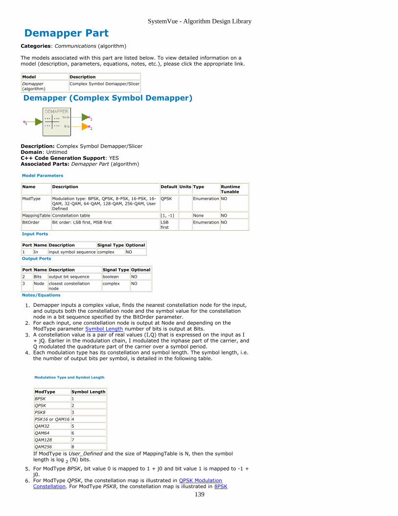
SystemVue - Algorithm Design Library
139
Demapper PartCategories: Communications (algorithm)
The models associated with this part are listed below. To view detailed information on amodel (description, parameters, equations, notes, etc.), please click the appropriate link.
Model Description
Demapper(algorithm)
Complex Symbol Demapper/Slicer
Demapper (Complex Symbol Demapper)
Description: Complex Symbol Demapper/SlicerDomain: UntimedC++ Code Generation Support: YESAssociated Parts: Demapper Part (algorithm)
Model Parameters
Name Description Default Units Type RuntimeTunable
ModType Modulation type: BPSK, QPSK, 8-PSK, 16-PSK, 16-QAM, 32-QAM, 64-QAM, 128-QAM, 256-QAM, UserDefined
QPSK Enumeration NO
MappingTable Constellation table [1, -1] None NO
BitOrder Bit order: LSB first, MSB first LSBfirst
Enumeration NO
Input Ports
Port Name Description Signal Type Optional
1 In input symbol sequence complex NO
Output Ports
Port Name Description Signal Type Optional
2 Bits output bit sequence boolean NO
3 Node closest constellationnode
complex NO
Notes/Equations
Demapper inputs a complex value, finds the nearest constellation node for the input,1.and outputs both the constellation node and the symbol value for the constellationnode in a bit sequence specified by the BitOrder parameter.For each input, one constellation node is output at Node and depending on the2.ModType parameter Symbol Length number of bits is output at Bits.A constellation value is a pair of real values (I,Q) that is expressed on the input as I3.+ jQ. Earlier in the modulation chain, I modulated the inphase part of the carrier, andQ modulated the quadrature part of the carrier over a symbol period.Each modulation type has its constellation and symbol length. The symbol length, i.e.4.the number of output bits per symbol, is detailed in the following table.
Modulation Type and Symbol Length
ModType Symbol Length
BPSK 1
QPSK 2
PSK8 3
PSK16 or QAM16 4
QAM32 5
QAM64 6
QAM128 7
QAM256 8
If ModType is User_Defined and the size of MappingTable is N, then the symbollength is log 2 (N) bits.
For ModType BPSK, bit value 0 is mapped to 1 + j0 and bit value 1 is mapped to -1 +5.j0.For ModType QPSK, the constellation map is illustrated in QPSK Modulation6.Constellation. For ModType PSK8, the constellation map is illustrated in 8PSK

SystemVue - Algorithm Design Library
140
Modulation Constellation. For ModType PSK16, the constellation map is illustrated in16PSK Modulation Constellation. The output symbols are assumed to be Gray coded.The symbol mappings for ModType QAM16, QAM32, QAM64, QAM128 and QAM2567.are described in the section 9 of [1], and their constellation maps are illustrated infigure 7-8 of [1].QAM constellations need definition only for quadrant 1. The constellation points in8.quadrants 2, 3 and 4 are derived from quadrant 1 by selecting the quadrant 1constellation value with the least significant bits of the desired symbol and rotatingthat constellation value by the amount selected by the two most significant bits ofthe desired symbol, b i b q, as specified in table Conversion of Constellation Points.
Conversion of Constellation Points
Quadrant Symbol Most Significant Bits ( b i b q ) Rotation
1 00 0
2 10 π/2
3 11 π
4 01 3π/2
16QAM, 32QAM, 64QAM, 128QAM and 256QAM constellation maps are illustrated in16 and 32QAM Constellation through 256QAM Constellation.When ModType is specified to User_Defined, a custom constellation is defined with9.MappingTable. The output symbol is mapped directly to a constellation point as a 0based index into MappingTable.
QPSK Modulation Constellation
8PSK Modulation Constellation
16PSK Modulation Constellation

SystemVue - Algorithm Design Library
141
16 and 32QAM Constellations
64QAM Constellation
128QAM Constellation
256QAM Constellation

SystemVue - Algorithm Design Library
142
See Mapper (algorithm).
References
EN 300 429, "Digital Video Broadcasting (DVB); Framing structure, channel coding1.and modulation for cable systems," V1.2.1, 1998-04.

SystemVue - Algorithm Design Library
143
Mapper PartCategories: Communications (algorithm)
The models associated with this part are listed below. To view detailed information on amodel (description, parameters, equations, notes, etc.), please click the appropriate link.
Model Description
Mapper(algorithm)
Complex SymbolMapper
Mapper (Complex Symbol Mapper)
Description: Complex Symbol MapperDomain: UntimedC++ Code Generation Support: YESAssociated Parts: Mapper Part (algorithm)
Model Parameters
Name Description Default Units Type RuntimeTunable
ModType Modulation type: BPSK, QPSK, 8-PSK, 16-PSK, 16-QAM, 32-QAM, 64-QAM, 128-QAM, 256-QAM, UserDefined
QPSK Enumeration NO
MappingTable Constellation table [1, -1] None NO
BitOrder Bit order: LSB first, MSB first LSBfirst
Enumeration NO
Input Ports
Port Name Description Signal Type Optional
1 In input bit sequence boolean NO
Output Ports
Port Name Description Signal Type Optional
2 Out output symbolsequence
complex NO
Notes/Equations
Mapper groups consecutive bits as specified by the BitOrder parameter in the input to1.form a symbol value which is mapped to a complex valued constellation point that isoutput.A constellation point is a pair of real values (I,Q) that is expressed on the output as I2.+ jQ. Later in the modulation chain, I modulates the inphase part of the carrier, andQ modulates the quadrature part of the carrier over a symbol period.Each modulation type has its constellation and symbol length. The symbol length, i.e.3.the number of input bits per symbol, is detailed in the following table.
Modulation Type and Symbol Length
ModType Symbol Length
BPSK 1
QPSK 2
PSK8 3
PSK16 or QAM16 4
QAM32 5
QAM64 6
QAM128 7
QAM256 8
If ModType is User_Defined and the size of MappingTable is N, then the symbollength is log 2 (N) bits.
For QPSK, PSK8, and PSK16 the mapping from bits to symbols is using Gray4.encoding. For QAM16, QAM32, QAM64, QAM128, and QAM256, Gray encoding is usedinside each quadrant.For ModType BPSK, bit value 0 is mapped to 1 + j0 and bit value 1 is mapped to -1 +5.j0.For ModType QPSK, the constellation map is illustrated in QPSK Constellation. For6.ModType PSK8, the constellation map is illustrated in 8PSK Constellation. For

SystemVue - Algorithm Design Library
144
ModType PSK16, the constellation map is illustrated in 16PSK Constellation.The symbol mappings for ModType QAM16, QAM32, QAM64, QAM128 and QAM2567.are described in the section 9 of [1], and their constellation maps are illustrated infigure 7-8 of [1].QAM constellations need definition only for quadrant 1. The constellation points in8.quadrants 2, 3 and 4 are derived from quadrant 1 by selecting the quadrant 1constellation value with the least significant bits of the input symbol and rotating thatconstellation value by the amount selected by the two most significant bits of theinput symbol, b i b q, as specified in table Conversion of Constellation Points.
Conversion of Constellation Points
Quadrant Symbol Most Significant Bits ( b i b q ) Rotation
1 00 0
2 10 π/2
3 11 π
4 01 3π/2
16QAM, 32QAM, 64QAM, 128QAM and 256QAM constellation maps are illustrated in16 and 32QAM Constellation through 256QAM Constellation.When ModType is specified to User_Defined, a custom constellation is defined with9.MappingTable. The input symbol is mapped directly to a constellation point as a 0based index into MappingTable.
QPSK Constellation
8PSK Constellation
16PSK Constellation

SystemVue - Algorithm Design Library
145
16 and 32QAM Constellation
64QAM Constellation
128QAM Constellation
256QAM Constellation

SystemVue - Algorithm Design Library
146
SeeMapper_M (algorithm)Demapper (algorithm)
References
EN 300 429, "Digital Video Broadcasting (DVB); Framing structure, channel coding1.and modulation for cable systems," V1.2.1, 1998-04.

SystemVue - Algorithm Design Library
147
AddGuard PartCategories: C++ Code Generation (algorithm), Communications (algorithm)
The models associated with this part are listed below. To view detailed information on amodel (description, parameters, equations, notes, etc.), please click the appropriate link.
Model Description
AddGuard(algorithm)
OFDM Symbol Guard Samples Inserter
AddGuard (OFDM Symbol Guard Samples Inserter)
Description: OFDM Symbol Guard Samples InserterDomain: UntimedC++ Code Generation Support: YESAssociated Parts: AddGuard Part (algorithm)
Model Parameters
Name Description Default Units Type Runtime Tunable
IFFTSize IFFT size 64 Integer NO
PreGuard Pre-guard length 16 Integer NO
PostGuard Post-guard length 0 Integer NO
Intersection Guard intersection length 0 Integer NO
Input Ports
Port Name Description Signal Type Optional
1 In Transmitted signal after IFFT complex NO
2 Window Window function real NO
Output Ports
Port Name Description Signal Type Optional
3 Out OFDM output data complex NO
Notes/Equations
Guard intervals are added to IFFT signals to form an OFDM symbol. Both Pre- and1.post-guard intervals are possible.IFFTSize specifies the input IFFT signal length.2.PreGuard specifies the pre-guard length. If PreGuard = 0, there is no pre-guard.3.PostGuard specifies the post-guard length. If PostGuard = 0, there is no post-guard.Intersection specifies the intersect length of two consecutive OFDM symbols. If4.Intersection = 0, there is no intersect between symbols. To protect the IFFT signals,Intersection cannot exceed PreGuard + PostGuard.IEEE 802 series (802.11a, 802.11g, 802.15.3a, 802.16a, 802.16d) and DVB-T5.standards do not include post-guard and intersection.For each OFDM symbol:6.
IFFTSize samples are input from pin In.PreGuard + IFFTSize + PostGuard samples are input from pin Window.PreGuard + IFFTSize + PostGuard - Intersection samples are output as theOFDM symbol.
A window function is input at pin Window for multiplying the output OFDM symbol. A7.non-window is created by providing a constant one at this pin.If an intersect does not exist, the windowed OFDM symbol is output.8.If an intersect does exist, the windowed OFDM symbol and the intersect of the9.previous OFDM symbol is added before output. The next intersect of the windowedOFDM symbol is saved for the next OFDM symbol.How an OFDM symbol is formed.10.
Inverse-Fourier-transformation creates the IFFT signal of time duration Tb(having IFFTSize samples) and constitute the useful symbol.A copy of the last time duration Tg (having PreGuard samples) of the usefulsymbol is added before the IFFT signal. This pre-guard is also called a cyclicprefix.A copy of the first time duration Tc (having PostGuard samples) of the usefulsymbol is added after the IFFT signal. This post-guard is also called a cyclicpostfix.The combined duration is referred to as symbol time Ts. OFDM Symbol Timewith Guard Interval illustrates this sequence.
OFDM Symbol Time with Guard Interval

SystemVue - Algorithm Design Library
148
How Intersection, PreGuard and PostGuard values form consecutive OFDM symbols11.for Case 1: Intersection > PreGuard and Intersection > PostGuard.
The second OFDM symbol is formed and multiplied by window.Intersect of the first and second OFDM symbols is then summed and outputfirst.Beginning after Intersection samples, the remaining segment of the secondOFDM symbol with length of PreGuard + IFFTSize + PostGuard - 2 ×Intersection is output.Last Intersection samples of the second OFDM symbol are saved as for the nextOFDM symbol.
Intersection > PreGuard, Intersection > PostGuard
Let the input be {0, 1, 2, 3, 4, 5} and {6, 7, 8, 9, 10, 11}, window is 1,IFFTSize = 6, PreGuard = 2, PostGuard = 2, Intersection = 3. With the stepsdescribed above, the output of the first and second OFDM symbol are {4, 5, 0,1, 2, 3, 4} and {15, 11, 7, 7, 8, 9, 10}, respectively. Case 1: Calculation forOutput illustrates the calculation.
Case 1: Calculation for Output
How Intersection, PreGuard and PostGuard values form consecutive OFDM symbols12.for Case 2: Intersection ≤ PreGuard and Intersection ≤ PostGuard.
This calculation is similar to Case 1.
Intersection ≤ PreGuard, Intersection ≤ PostGuard
Let the input be {0, 1, 2, 3, 4, 5} and {6, 7, 8, 9, 10, 11}, window is 1,IFFTSize = 6, PreGuard = 3, PostGuard = 3, Intersection = 2. The output of thefirst and second OFDM symbols are {3, 4, 5, 0, 1, 2, 3, 4, 5, 0} and {10, 12,11, 6, 7, 8, 9, 10, 11, 6}, respectively. Case 2: Calculation for Output illustratesthe calculation.
Case 2: Calculation for Output
References
IEEE Standard 802.11a-1999, "Part 11: Wireless LAN Medium Access Control (MAC)1.and Physical Layer (PHY) specifications: High-speed Physical Layer in the 5 GHzBand," 1999.ETSI TS 101 475 v1.1.1, "Broadband Radio Access Networks (BRAN); HIPERLAN Type2.2; Physical (PHY) layer," April, 2000.ARIB-JAPAN, Terrestrial Integrated Services Digital Broadcasting (ISDB-T);3.

SystemVue - Algorithm Design Library
149
Specification of Channel Coding, Frame Structure and Modulation, Sept.1998.ETSI, Digital Video Broadcasting (DVB); Framing structure, channel coding and4.modulation for digital terrestrial television. EN300 744 v1.2.1, EuropeanTelecommunication Standard, July 1999.IEEE P802.15-03/268r1, "Multi-band OFDM Physical Layer Proposal for IEEE 802.155.Task Group 3a," September 2003.IEEE P802.16-REVd/D2-2003, "Draft IEEE Standard for Local and metropolitan area6.networks Part 16: Air Interface for Fixed Broadband Wireless Access Systems," 2003.

SystemVue - Algorithm Design Library
150
BCH_Decoder PartCategories: C++ Code Generation (algorithm), Communications (algorithm)
The models associated with this part are listed below. To view detailed information on amodel (description, parameters, equations, notes, etc.), please click the appropriate link.
Model Description
BCH_Decoder(algorithm)
Binary primitive BCH decoder

SystemVue - Algorithm Design Library
151
BCH_Decoder
Description: Binary primitive BCH decoderDomain: UntimedC++ Code Generation Support: YESAssociated Parts: BCH Decoder Part (algorithm)
Model Parameters
Name Description Default Units Type RuntimeTunable
M The root of generation polynomial is defined inGF(2^M), primitive codeword length N=2^M-1
3 Integer NO
K Primitive message length (Unshortened) 4 Integer NO
T Error correction capability 1 Integer NO
CodeLength Shortened codeword length ( <=2^M-1 ), set 0 forunshortened code
0 Integer NO
PrimPoly Primitive polynomial in the form of integer (default[]), binary vector or power vector of non-zero item
[] Integerarray
NO
Erase there is erased bits or not in undecoded code: NO,YES
NO Enumeration NO
ErasePosition index array of erased bits (from [0,CodeLength-1]),valid if Erase==YES and pin EraseFlag isdisconnected
[] Integerarray
NO
Input Ports
Port Name Description Signal Type Optional
1 Code Uncoded binary codeword int NO
2 EraseFlag Specifying the corresponding bits is erased (1) or not (0) int YES
Output Ports
Port Name Description Signal Type Optional
3 Msg Decoded binary messageword int NO
Notes/Equations
This model performs the decoding of primitive binary BCH (Bose-Chaudhuri-1.Hocquengham) systematic code.The primitive message length, is represented by K, and the primitive codeword2.length, 2M-1, is represented by N. For shortened code, Ks and Ns represent theshortened message length and codeword length respectively.Each run, it consumes Ns = min(N,CodeLength) input codeword bits and output Ks =3.K+min(0,CodeLength-2M-1) decoded message bits. CodeLength=0 is treated thesame as CodeLength=N.The primitive polynomial of the Galois Field GF(2M), p(x) = 1+p(2)*x+p(3)*x24.
+...+p(M)*xM-1+xM, is set by array PrimPoly in three ways. If p(x)= 1+x+x4, i.e.p(x) = 1*x0+1*x1+0*x2+0*x3+1*x4, PrimPoly can be
an array consists of the order of x whose coefficients are 1, i.e.
[0,1,4]
an array consists of all polynomial coefficients, from the lowest power tothe highest power, i.e.
[1,1,0,0,1]
an integer p(2), i.e.
19
NoteIf PrimPoly is set to [], the default primitive polynomials shown below shall be used
The relationship of T and code generation polymonial g(x)5.
T is the error correction capability, i.e. the number of reducible error bits inthe received codeword.

SystemVue - Algorithm Design Library
152
2*T+1 equals to the minimum distance between different codewords, orthe number of 1's in the coefficient array of g(x).
Decoding algorithm6.Constructing the codeword polynomial
r(x) = r(0)*xNs-1 + r(1)*xNs-2 + ... + r(Ns-2)*x + r(Ns-1)
from un-decoded input (r(0) is the first input bit)
r = [r(0), r(1), ..., r(Ns-1)]Calculating the syndrome S
S(i) = r(αi), i=1,2,...,T*2, α is a primitive element of GF(2M)
If {S(i)} are all zeros, i.e. no (reducible) errors, picking up [r(0), r(1),..., r(Ks-1)] as the decoded message and return. Otherwise, goingforward to the next step
Calculating error location polynomial with Berlekamp-Massey algorithm
σ(x) = σ(0) + σ(1)*x + σ(2)*x2 + ... + σ(v)*xv, v≤T
by filling the iterative table
u σu(x) du lu u-lu
-1 1 1 0 -1
0 1 S1 0 0
1
2
...
2T
with the following iteration method
Assuming the result of the uth iteration is
σu(x) = σu(0) + σu(1)*x + σu(2)*x2 + ... + σu(lu)*xlu
to deduce σu+1(x), calculate the uth discrepancy
du = Su+1 + σu(1)Su + σu(2)Su-1 + ... + σu(lu)Su+1-lu
If du==0,
σu+1(x) = σu(x)
otherwise, search σρ(x) satisfying ρ<u, dρ≠0 and ρ-lρ=max{i-li}, -
1≤i<u, and rewrite σu+1(x) as
σu+1(x) = σu(x) + du dρ-1 xu-ρ σρ(x)
Calculating the error locations with Chien Search
Create a all-zero array e = [e(0), e(1), ..., e(Ns-1)]
Evaluate σ(x) with {αi+1, N-Ns≤i<N}. If σ(αi)==0, i.e. r(i-(N-Ns)) is aerror bit, set e(i) to 1.
Correcting error bits with error array e obtained above and get the decodedoutput bits
udec = [r(0), r(1), ..., r(Ks-1)] + [e(0), e(1), ..., e(Ks-1)]
If Erase is YES, the decoder shall perform a decoding with erased bits.7.The positions of erased bits is set by ErasePosition consisting of not more than2T digits with each in the range of [0,CodeLength)If the EraseFlag pin is connected, parameter ErasePosition shall be ignored.EraseFlag should has the same length as Input and in which 1 represents anerased bits and 0 represents not.The decoder decode the codeword twice by replacing the erased bits with logic1's and 0's respectively. Decoded message is obtained from one of the twodecoded codewords which has the smaller distance from the uncoded codewords(excluding the erased positions).
Default primitive polynomials8.
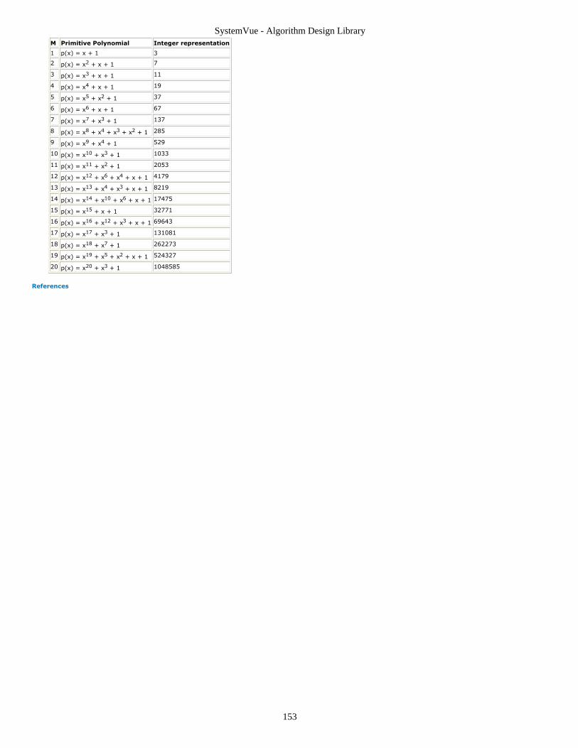
SystemVue - Algorithm Design Library
153
M Primitive Polynomial Integer representation
1 p(x) = x + 1 3
2 p(x) = x2 + x + 1 7
3 p(x) = x3 + x + 1 11
4 p(x) = x4 + x + 1 19
5 p(x) = x5 + x2 + 1 37
6 p(x) = x6 + x + 1 67
7 p(x) = x7 + x3 + 1 137
8 p(x) = x8 + x4 + x3 + x2 + 1 285
9 p(x) = x9 + x4 + 1 529
10 p(x) = x10 + x3 + 1 1033
11 p(x) = x11 + x2 + 1 2053
12 p(x) = x12 + x6 + x4 + x + 1 4179
13 p(x) = x13 + x4 + x3 + x + 1 8219
14 p(x) = x14 + x10 + x6 + x + 1 17475
15 p(x) = x15 + x + 1 32771
16 p(x) = x16 + x12 + x3 + x + 1 69643
17 p(x) = x17 + x3 + 1 131081
18 p(x) = x18 + x7 + 1 262273
19 p(x) = x19 + x5 + x2 + x + 1 524327
20 p(x) = x20 + x3 + 1 1048585
References

SystemVue - Algorithm Design Library
154
BCH_Encoder PartCategories: C++ Code Generation (algorithm), Communications (algorithm)
The models associated with this part are listed below. To view detailed information on amodel (description, parameters, equations, notes, etc.), please click the appropriate link.
Model Description
BCH_Encoder(algorithm)
Binary BCH Encoder

SystemVue - Algorithm Design Library
155
BCH_Encoder
Description: Binary BCH EncoderDomain: UntimedC++ Code Generation Support: YESAssociated Parts: BCH Encoder Part (algorithm)
Model Parameters
Name Description Default Units Type RuntimeTunable
M The root of generation polynomial is defined inGF(2^M), primitive codeword length N=2^M-1
3 Integer NO
K Primitive message length (Unshortened) 4 Integer NO
MsgLength Shortened message length [0,K], set 0 (or K) forunshortened code
0 Integer NO
GenPoly Code generation polynomial (if g( x)=1+X+X^3,GenPoly=[0,1,3] or [1,1,0,1])
[0,1,3] Integerarray
NO
Input Ports
Port Name Description Signal Type Optional
1 Msg Uncoded binarymessage
int NO
Output Ports
Port Name Description Signal Type Optional
2 Code Encoded binarycodeword
int NO
Notes/Equations
This model performs the encoding of binary BCH (Bose-Chaudhuri-Hocquengham)1.systematic code.The primitive message length, is represented by K, and the primitive codeword2.length, 2M-1, is represented by N. For shortened code, Ks and Ns represent theshortened message length and codeword length respectively.Each run, it consumes Ks = min(K,MsgLength) input message bits and output Ns =3.N+min(0,MsgLength-K) codeword bits. MsgLength=0 is treated the same asMsgLength=K.The code generation polynomial, g(x), with the highest order xN-K, is set by array4.GenPoly in three ways.
1-D array of the order of x whose coefficients are 1. For instance, if g(x)=1+x+x3, i.e. g(x) = 1*x0+1*x1+0*x2+1*x3, GenPoly should be [0,1,3]. Thenumber of parity bits is the highest power of g(x).1-D array consists of all polynomial coefficients, from lowest power to highestpower. If g(x)= 1+x+x3, i.e. g(x) = 1*x0+1*x1+0*x2+1*x3, GenPoly should be[1,1,0,1].2-D array consists of the polynomial coefficients of g(x)'s factor polynomialswhose highest power ≤M. For instance, if g(x) = (1+x+x4) * (1+x+x2+x3+x4) *(1+x+x2), GenPoly can be set as a 3 x (M+1) array
[1,1,0,0,1; 1,1,1,1,1; 1,1,1,0,0]
Coding process5.Constructing the message polymonial
u(x) = u(0)*xKs-1 + u(1)*xKs-2 + ... + u(Ks-2)*x + u(Ks-1)
from input Msg (rewrite as u, u(0) is the first input bit)
u = [u(0), u(1), ..., u(Ks-1)]Dividing xNs-Ksu(x) by g(x) and obtaining the remainer polynomial
b(x) = xNs-Ksu(x)/g(x) = b(0)*xNs-Ks-1 + b(1)*xNs-Ks-2 + ... + b(Ns-Ks-2)*x + b(Ns-Ks-1)
Combining u(x) and g(x) to obtain the codeword polynomial c(x) (c(0) is thefirst output bit)

SystemVue - Algorithm Design Library
156
c(x) = xNs-Ksu(x) + b(x) = c(0)*xNs-1 + c(1)*xNs-2 + ... + c(Ns-2)*x+ c(Ns-1)
and the codeword array
c = [c(0), c(1), ... c(Ns-1)] = [u(0), u(1), ... u(Ks-1), b(0), b(1), ...,b(Ns-Ks-1)]
References

SystemVue - Algorithm Design Library
157
CoderRS PartCategories: C++ Code Generation (algorithm), Communications (algorithm)
The models associated with this part are listed below. To view detailed information on amodel (description, parameters, equations, notes, etc.), please click the appropriate link.
Model Description
CoderRS(algorithm)
Reed Solomon Encoder
CoderRS (Reed Solomon Encoder)
Description: Reed Solomon EncoderDomain: UntimedC++ Code Generation Support: YESAssociated Parts: CoderRS Part (algorithm)
Model Parameters
Name Description Default Units Type RuntimeTunable
GF Galois field size (2^GF) 8 Integer NO
CodeLength Length of output codeword 255 Integer NO
MessageLength Length of input message symbols 223 Integer NO
PrimPoly Coefficients of primitive polynonial. PrimPolymust be the coefficients of the m order ofpolynomial
[1, 0, 1, 1, 1,0, 0, 0, 1]
Integerarray
NO
Root First root of generator polynomial 1 Integer NO
Input Ports
Port Name Description Signal Type Optional
1 in information symbol int NO
Output Ports
Port Name Description Signal Type Optional
2 out systematical code int NO
Notes/Equations
The CoderRS model implements a Reed-Solomon (RS) encoder.1.This model reads k samples from input in and writes n samples to output out.2.RS codes are a class of block codes that operate on non-binary symbols. The symbols3.are formed from m bits of a binary data stream. A code block is then formed with n =2 m - 1 symbols. In each block, k symbols are formed from the encoder input and (n- k) parity symbols are added. The code is thus a systematic code. The rate of thecode is k/n, and the code is able to correct up to t = (n - k - 1)/2 or (n - k)/2 symbolerrors in a block, depending on whether n - k is odd or even. For example, the codeused in the WCDMA [1] data transmission system is a (36,32) code shortened fromRS code (255,251) defined on Galois Field (2 8). A shortened code can be formed bytaking 32 input symbols, padding them out with 219 all zero symbols to form 251symbols, and then encoding with a RS code (255,251). The 219 fixed symbols arethen discarded prior to transmission. The input pin consumes k tokens and the outputpin produces n tokens for each firing.Implementation4.The code format is: RS code (n, k), defined on Galois Field (2 m).Galois Field GeneratorGalois Fields are set up according to the number of bits per symbol and the numberof symbols per block.Generate GF (2 m) from the irreducible primitive polynomial. It is defined as thepolynomial of least degree, with coefficients in GF(2) and a highest degree coefficientequal to 1. The polynomial is always of degree m.The elements of Galois Field can have two representations: exponent or polynomial.Let α represent the root of the primitive polynomial p(x). Then in GF(2 m), for any 0 ≤ i ≤ 2 m - 2
where the binary vector (bi(0), bi(1),..., bi(m_-1)) is the representation of theinteger polynomial[i]. Now exponent[i] is the element whose polynomialrepresentation is (bi(0), bi(1),..., bi(m-1)), and exponent[polynomial[i]] = i.

SystemVue - Algorithm Design Library
158
Polynomial representation is convenient for addition, exponent representation formultiplication.RS EncoderThe RS generator polynomial is generally defined as
where t is the correctable error number. It can be reduced to a 2t order of polynomial
Encoding is done by using a feedback shift register with appropriate connectionsspecified by the element g i . The encoded symbol is then
where in(x) is the polynomial representation of the input data, parity(x) is thepolynomial of the parity symbol.The RS encoder diagram is illustrated in Reed Solomon Encoder. Figure: Reed Solomon Encoder
See Also:
DecoderRS (algorithm)
References
NTT Mobile Communications Network Inc. "Specifications for W-CDMA Mobile1.Communication System Experiment", October 9, 1997.S. Lin, D. J. Costello, Error Control Coding Fundamentals and Applications, 1983.2.

SystemVue - Algorithm Design Library
159
ConvolutionalCoder PartCategories: C++ Code Generation (algorithm), Communications (algorithm)
The models associated with this part are listed below. To view detailed information on amodel (description, parameters, equations, notes, etc.), please click the appropriate link.
Model Description
ConvolutionalCoder(algorithm)
ConvolutionalCoder
ConvolutionalCoder (ConvolutionalCoder)
Description: Convolutional CoderDomain: UntimedC++ Code Generation Support: YESAssociated Parts: ConvolutionalCoder Part (algorithm)
Model Parameters
Name Description Default Units Type RuntimeTunable
CodingRate Coding rate: rate_1_2, rate_1_3, rate_1_4,rate_1_5, rate_1_6, rate_1_7, rate_1_8
rate_1_2 Enumeration NO
ConstraintLength Constraint length 7 Integer NO
Polynomial Generator polynomial [91,121]
Integerarray
NO
ZeroTail Zero tail used to convert convolutional codeto block code: NO, YES
NO Enumeration NO
BitSequenceLength Length of bit squence not including tail bits 88 Integer NO
Input Ports
Port Name Signal Type Optional
1 In boolean NO
Output Ports
Port Name Signal Type Optional
2 Out boolean NO
Notes/Equations
The ConvolutionalCoder model convolutionally encodes the input information1.sequence bit-by-bit.This model reads 1 sample from input In and writes R samples to output Out. R = 2,2.3, 4, 5, 6, 7, or 8 when CodingRate = rate_1_2, rate_1_3, rate_1_4, rate_1_5,rate_1_6, rate_1_7, or rate_1_8 respectively.A convolutional code is generated by passing the information sequence to be3.transmitted through a linear finite-state shift register. The shift register generallyconsists of K(k-bit) stages and n linear algebraic function generators. Input data tothe encoder (assumed to be binary) is shifted into (and along) the shift register k bitsat a time. The number of output bits for each k-bit input sequence is n bits.Therefore, the code rate is defined as R c = k /n, which is consistent with the code
rate definition for a block code. The K parameter is called the constraint length of theconvolutional code.CodingRate (R c) is the ratio of input bit (k) and output bits (n). ConvolutionalCoder4.
supports the 1/n coding rate only, which implements an R c = 1/n rate(n = 2, 3, 4, 5,
6, 7, 8) convolution for input data.Convolutional codes with k /n (k > 1) are not supported by this component because:coding and decoding will be more complex; and, even convolutional codes with a k /n(k > 1) coding rate are used that are typically implemented by puncturing theconvolutional code with a 1/n coding rate.ConstraintLength (K) represents shift register stages.5.Polynomial is the generator function of the convolutional code. In general, the6.generator matrix for a convolutional code is semi-infinite since the input sequence issemi-infinite. As an alternative to specifying the generator matrix, a functionallyequivalent representation is used in which a set of n vectors is specified, one vectorfor each n modulo-2 adder. A 1 in the ith position of the vector indicates that thecorresponding stage in the shift register is connected to the modulo-2 adder; 0 in agiven position indicates that no connection exists between that stage and themodulo-2 adder.
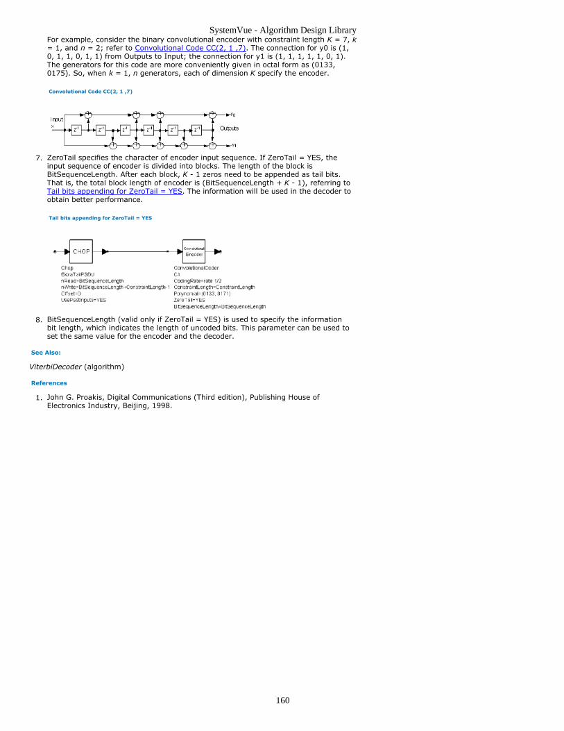
SystemVue - Algorithm Design Library
160
For example, consider the binary convolutional encoder with constraint length K = 7, k= 1, and n = 2; refer to Convolutional Code CC(2, 1 ,7). The connection for y0 is (1,0, 1, 1, 0, 1, 1) from Outputs to Input; the connection for y1 is (1, 1, 1, 1, 1, 0, 1).The generators for this code are more conveniently given in octal form as (0133,0175). So, when k = 1, n generators, each of dimension K specify the encoder.
Convolutional Code CC(2, 1 ,7)
ZeroTail specifies the character of encoder input sequence. If ZeroTail = YES, the7.input sequence of encoder is divided into blocks. The length of the block isBitSequenceLength. After each block, K - 1 zeros need to be appended as tail bits.That is, the total block length of encoder is (BitSequenceLength + K - 1), referring toTail bits appending for ZeroTail = YES. The information will be used in the decoder toobtain better performance.
Tail bits appending for ZeroTail = YES
BitSequenceLength (valid only if ZeroTail = YES) is used to specify the information8.bit length, which indicates the length of uncoded bits. This parameter can be used toset the same value for the encoder and the decoder.
See Also:
ViterbiDecoder (algorithm)
References
John G. Proakis, Digital Communications (Third edition), Publishing House of1.Electronics Industry, Beijing, 1998.

SystemVue - Algorithm Design Library
161
CRC_Coder PartCategories: Communications (algorithm)
The models associated with this part are listed below. To view detailed information on amodel (description, parameters, equations, notes, etc.), please click the appropriate link.
Model Description
CRC_Coder(algorithm)
CRC Coder
CRC_Coder (CRC Coder)
Description: CRC CoderDomain: UntimedC++ Code Generation Support: NOAssociated Parts: CRC Coder Part (algorithm)
Model Parameters
Name Description Default Units Type RuntimeTunable
Range
ParityPosition Parity bits position: Tail, Head Tail Enumeration NO
ReverseData Reverse the data sequence: NO,YES
NO Enumeration NO
ReverseParity Peverse the parity bits: NO, YES NO Enumeration NO
ComplementParity Complement parity bits: NO, YES NO Enumeration NO
MessageLength Input message length 172 Integer NO [1:∞)
InitialState Initial state of encoder 0 Integer NO [0:∞)
Polynomial Generator polynomial 7955 Integer NO [3:∞)
Input Ports
Port Name Description Signal Type Optional
1 In input data boolean NO
Output Ports
Port Name Description Signal Type Optional
2 Out output data boolean NO
Notes/Equations
This component is used to add CRC bits to the input information.1.Each firing, (MessageLength + CRCLength) tokens are produced whenMessageLength tokens are consumed. CRCLength is the length of CRC bits that isdetermined by Polynomial, where 2CRCLength ≤ Polynomial ≤ 2CRCLength+1 .CRC bits can be added to the head or the tail of the information bits by setting2.ParityPosition. The order of CRC bits and the order of information bits can bereversed by setting ReverseData and ReverseParity.CRC Bit Calculation as shown below is an example of a CRC encoder in CDMA2000,3.where g(x) = x 6 + x 2 + x + 1, and Polynomial is hex 0x47. The CRC bits are addedafter the information bits; the order of the CRC and information bits are not reversed.
Initially, all shift register elements are set to the InitialState and the switchesare set in the up position.The register is clocked the number of times equal to MessageLength.Switches are then set in the down position so that the output is a modulo-2addition with a 0 and the successive shift register inputs are 0.The register is clocked an additional number of times equal to CRCLength andthe CRC bits are output.

SystemVue - Algorithm Design Library
162
References
TIA/EIA/IS-2000.2 (PN-4428), Physical Layer Standard for cdma2000 Spread1.Spectrum Systems, July 1999.

SystemVue - Algorithm Design Library
163
CRC_Decoder PartCategories: Communications (algorithm)
The models associated with this part are listed below. To view detailed information on amodel (description, parameters, equations, notes, etc.), please click the appropriate link.
Model Description
CRC_Decoder(algorithm)
CRCDecoder
CRC_Decoder (CRC Decoder)
Description: CRC DecoderDomain: UntimedC++ Code Generation Support: NOAssociated Parts: CRC Decoder Part (algorithm)
Model Parameters
Name Description Default Units Type RuntimeTunable
Range
ParityPosition Parity bits position: Tail, Head Tail Enumeration NO
ReverseData Reverse the data sequence: NO,YES
NO Enumeration NO
ReverseParity Peverse the parity bits: NO, YES NO Enumeration NO
ComplementParity Complement parity bits: NO, YES NO Enumeration NO
MessageLength Input message length 172 Integer NO [1:∞)
InitialState Initial state of encoder 0 Integer NO [0:∞)
Polynomial Generator polynomial 7955 Integer NO [3:∞)
Input Ports
Port Name Description Signal Type Optional
1 In input data boolean NO
Output Ports
Port Name Description Signal Type Optional
2 Out output data boolean NO
3 Parity Parity check int NO
Notes/Equations
This component is used to check the CRC bits for CRC frame errors.1.Each firing, (MessageLength + CRCLength) tokens are consumed whenMessageLength tokens and one parity token are produced. CRCLength is the CRC bitlength determined by Polynomial, where 2CRCLength ≤ Polynomial ≤ 2CRCLength+1.The message part of the input data is sent to a CRC encoder that has the same2.Polynomial value as the encoder (CRC_Coder). The CRC bits are then compared withthe CRC bits in the input data. If these are the same, the CRC check is passed.

SystemVue - Algorithm Design Library
164
DecoderRS PartCategories: Communications (algorithm)
The models associated with this part are listed below. To view detailed information on amodel (description, parameters, equations, notes, etc.), please click the appropriate link.
Model Description
DecoderRS(algorithm)
Reed Solomon Decoder
DecoderRS (Reed Solomon Decoder)
Description: Reed Solomon DecoderDomain: UntimedC++ Code Generation Support: NOAssociated Parts: DecoderRS Part (algorithm)
Model Parameters
Name Description Default Units Type RuntimeTunable
Range Symbol
GF Galois field size(2^GF)
8 Integer NO [2:30] m
CodeLength Length of inputcodewords
255 Integer NO [3:2<sup>m</sup>-1] n
MessageLength Length of outputmessage symbols
223 Integer NO [1:CodeLength-2] k
PrimPoly Coefficients ofprimitivepolynomial
[1, 0, 1, 1,1, 0, 0, 0,1]
Integerarray
NO † p
Root First root ofgeneratorpolynomial
1 Integer NO [0:2<sup>m</sup>-1- (n - k)]
m0
Input Ports
Port Name Description Signal Type Optional
1 in received symbol int NO
Output Ports
Port Name Description Signal Type Optional
2 out decodedsymbol
int NO
Notes/Equations
The DecoderRS model implements a Reed-Solomon (RS) decoder.1.This model reads n samples from input in and writes k samples to output out.2.The RS decoding is performed via the Berlekamp iterative algorithm [2].3.The Berlekamp iterative algorithm locates the error in RS code and generates an4.error location polynomial. By finding the root of the error location polynomial, theerror position can be determined. If decoding is successful, the information symbolsare output; otherwise, the received data is unaltered.Decoding routines are described here.5.For the shortened code, the same number of symbols 0 is inserted into the sameposition as CoderRS and a Reed Solomon decoder is used to decode the block. Afterdecoding, the padded symbols are discarded, leaving the desired informationsymbols.Syndromes indicate erroneous situations. When the generator polynomial g(x) andthe received codeword represented by r(x) are given, one or more errors haveoccurred during transmission of an encoded block.Let
where v(x) is the polynomial representation of the transmitted symbol.
where r(x) is the polynomial representation of the received symbol.Then
where e(x) denotes the error patterns.If r i - v i, then e i = 0; else e i = 1.

SystemVue - Algorithm Design Library
165
Remember thatv(x) = g(x)Q(x)where Q(x) is the quotient.So if α i is the root of g(x) , then v(α i) = 0 and r(α i) = e(α i).Now there is a simple procedure for checking the occurrence of errors at the receiver:Calculate syndromes s(i), the syndromes are decided by the error patterns:
If one or more of the syndromes are not equal to zero, one or more symbol errorsoccur in the received data. For example, if
are roots of g(x), then
.
.
.
Syndromes are used to find the error location polynomial.Given the syndromes s(i), the decoding algorithm will synthesize an error locationpolynomial. The roots of the polynomial indicate the error positions.Assuming the received symbols have v symbol errors, the syndromes arerepresented as:
.
.
.
where the error location is
and
Now the error location polynomial is defined as
The Berlekamp iterative algorithm is used to construct this polynomial, which is thekey to RS decoding.The algorithm is described here without proof; for more information, see Ref. [1].An iterative table will be filled.
-1 1 1 0 -1
0 1 s 1 0 0
1
2 ... , 2t
where
is the iterative step number
is the mth step iterative difference
is the order of If
then
and
If

SystemVue - Algorithm Design Library
166
search for lines in the table to find step p in which d p ≠ 0 and the value of p - l p is
the maximum, then
and
For the two conditions
Iterate until the last line of the table Ω (2 t) (x) is calculated. If the order of thepolynomial is greater than t (which means the received codeword block has morethan t errors) the error cannot be corrected.For non-binary codes, the error values must be known.The minimum order polynomial is iteratively solved to obtain the least number ofroots (error location number). The inverse element of the root indicates the errorlocation.The error value is calculated based on the Ref. [2] equation
where
Then,
See Also:
CoderRS (algorithm)
References
E.R. Berlekamp, Algebraic Coding Theory, McGraw-Hill, New York, 1968.1.S. Lin, D. J. Costello, Error Control Coding Fundamentals and Applications, 1983.2.

SystemVue - Algorithm Design Library
167
Deinterleaver802 PartCategories: Communications (algorithm)
The models associated with this part are listed below. To view detailed information on amodel (description, parameters, equations, notes, etc.), please click the appropriate link.
Model Description
Deinterleaver802(algorithm)
IEEE 802 Deinterleaver
Deinterleaver802 (IEEE 802 Deinterleaver)
Description: IEEE 802 DeinterleaverDomain: UntimedC++ Code Generation Support: NOAssociated Parts: Deinterleaver802 Part (algorithm)
Model Parameters
Name Description Default Units Type Runtime Tunable Range
s Modular factor of interleaving 1 Integer NO [1:∞)
l Divisor factor of interleaving 16 Integer NO [1:∞)
NCBPS Number of coded bits per OFDMsymbol
48 Integer NO [1:∞)
Input Ports
Port Name Description Signal Type Optional
1 In Input real NO
Output Ports
Port Name Description Signal Type Optional
2 Out Output real NO
Notes/Equations
The Deinterleaver802 model performs deinterleaving based on IEEE 802 standards. It1.performs the inverse of the Interleaver802 model.This model reads N CBPS samples from input In and writes N CBPS samples to the2.
output Out.N CBPS is the number of coded bits in a single OFDM symbol and is defined in the
table below.Deinterleaving is defined by a two-step permutation; j is used to denote the index of3.the original received bit before the first permutation; i is used to denote the indexafter the first (and before the second) permutation; k is used to denote the indexafter the second permutation, before delivering the coded bits to the convolutional(Viterbi) decoder.The first permutation is defined byi = s × floor(j/s) + (j + floor(l × j/ N CBPS )) mod s j = 0, 1, ... N CBPS - 1
The function floor (.) denotes the largest integer not exceeding the parameterThe second permutation is defined byk = l × i - (N CBPS - 1)floor(l × i/N CBPS) i = 0, 1, ... N CBPS - 1
In the equations, s is the modular factor and l is the divisor factor; these are variableparameters and their values depend on which standard the model is used for.If this model is used for IEEE 802.11 and HIPERLAN/2s = max (N BPSC/2, 1), l = 16
whereN BPSC and N CBPS are determined by data rates given in IEEE 802.11 and
HIPERLAN/2 Rate Dependent Values.If this model is used for IEEE 802.16s = N BPSC /2, 1) l = 12
where N BPSC and N CBPS are determined by block sizes given in IEEE 802.16 Bit
Interleaver Block Sizes (NCBPS / NBPSC).
IEEE 802.11 and HIPERLAN/2 Rate Dependent Values

SystemVue - Algorithm Design Library
168
Data Rate(Mbps)
Modulation CodingRate (R)
Coded Bits perSubcarrier(NBPSC)
Coded Bits perOFDM Symbol(NCBPS)
Data Bits per OFDMSymbol (NDBPS)
6 BPSK 1/2 1 48 24
9 BPSK 3/4 1 48 36
12 QPSK 1/2 2 96 48
18 QPSK 3/4 2 96 72
24 (IEEE802.11a)
16QAM 1/2 4 192 96
27(HIPERLAN/2)
16QAM 9/16 4 192 108
36 16QAM 3/4 4 192 144
48 (IEEE802.11a)
64QAM 2/3 6 288 192
54 64QAM 3/4 6 288 216
IEEE 802.16 Bit Interleaver Block Sizes (N CBPS / N BPSC)
Modulation 16 Subchannels (Default) 8 Subchannels 4 Subchannels 2 Subchannels 1 Subchannel
QPSK 384/2 192/2 96/2 48/2 24/2
16QAM 768/4 384/4 192/4 96/4 48/4
64QAM 1152/6 576/6 288/6 144/6 72/6
See Also:
Interleaver802 (algorithm)
References
IEEE Standard 802.11a-1999, "Part 11: Wireless LAN Medium Access Control (MAC)1.and Physical Layer (PHY) specifications: High-speed Physical Layer in the 5 GHzBand," 1999.ETSI TS 101 475 v1.1.1, "Broadband Radio Access Networks (BRAN); HIPERLAN Type2.2; Physical (PHY) layer," April, 2000.IEEE P802.16-REVd/D2-2003," Part 16 Air Interface for Fixed Broadcast Wireless3.Access Systems".

SystemVue - Algorithm Design Library
169
DeScrambler PartCategories: Communications (algorithm)
The models associated with this part are listed below. To view detailed information on amodel (description, parameters, equations, notes, etc.), please click the appropriate link.
Model Description
DeScrambler(algorithm)
Bit Sequence Descrambler
DeScrambler (Bit Sequence Descrambler)
Description: Bit Sequence DescramblerDomain: UntimedC++ Code Generation Support: NOAssociated Parts: DeScrambler Part (algorithm)
Model Parameters
Name Description Default Units Type RuntimeTunable
Range
Polynomial Generator polynomial for the shift register -decimal, octal, or hex integer
147457 Integer NO (0:∞)
ShiftReg Initial state of the shift register - decimal, octal,or hex integer
1 Integer NO (-∞:∞)
Input Ports
Port Name Description Signal Type Optional
1 input input bit sequence (zero ornonzero)
boolean NO
Output Ports
Port Name Description Signal Type Optional
2 output output bit sequence (zero orone)
boolean NO
Notes/Equations
This component descrambles the input bit sequence using a feedback shift register.1.The taps of the feedback shift register are given by the Polynomial parameter.This is a self-synchronizing descrambler that will exactly reverse the operation of theScrambler component if the corresponding parameter values of Scrambler andDeScrambler are the same.A self-synchronized descrambler is shown in Self-Synchronized Descrambler.Figure:Self-Synchronized Descrambler
See also, Scrambler (algorithm).2.
References
E. A. Lee and D. G. Messerschmitt, Digital Communication, Second Edition, Kluwer1.Academic Publishers, 1994, pp. 595-603.

SystemVue - Algorithm Design Library
170
FMPulseTrain PartCategories: Communications (algorithm)
The models associated with this part are listed below. To view detailed information on amodel (description, parameters, equations, notes, etc.), please click the appropriate link.
Model Description
FMPulseTrain(algorithm)
Frequency modulated pulsetrain
FMPulseTrain
Description: Frequency modulated pulse trainDomain: TimedC++ Code Generation Support: NOAssociated Parts: FMPulseTrain Part (algorithm)
Model Parameters
Name Description Default Units Type Runtime Tunable Range
Frequency Nominal frequency of the pulse train 20e3 Hz Float NO (0:∞)
InitialPhase Initial phase 0 deg Float YES (-∞:∞)
FreqSensitivity Frequency deviation sensitivity inHz/Volt
1e5 Float YES (-∞:∞)
Amplitude Amplutide of the pulse train 1 V Float YES (-∞:∞)
PulseWidth Time width of the output pulse train 1e-6 s Float YES (0:∞)
Input Ports
Port Name Description Signal Type Optional
1 input input real NO
Output Ports
Port Name Description Signal Type Optional
2 output output real NO
Notes/Equations
FMPulseTrain generates a frequency modulated pulse train.1.For every input, there is one output.2.Consider a phasor P(t) operating at 3.radians per second.P(t) is P(0) _ where P(0) is InitialPhase.4.If P(t) crosses for integer n within the last time step, a pulse is generated.5.A pulse has Amplitude value and persists PulseWidth seconds. No pulse is6.represented by a zero output.PulseWidth is rounded to the nearest time step and is forced to be at least one time7.step.Pulses may overlap, however the most recently generated pulse determines the next8.no pulse time.
See also: Modulator (algorithm).

SystemVue - Algorithm Design Library
171
GoldCode PartCategories: C++ Code Generation (algorithm), Communications (algorithm)
The models associated with this part are listed below. To view detailed information on amodel (description, parameters, equations, notes, etc.), please click the appropriate link.
Model Description
GoldCode(algorithm)
Gold Code Generator
GoldCode
Description: Gold Code GeneratorDomain: UntimedC++ Code Generation Support: YESAssociated Parts: GoldCode Part (algorithm)
Model Parameters
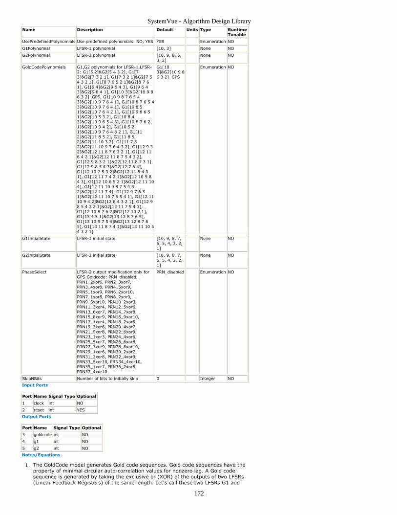
SystemVue - Algorithm Design Library
172
Name Description Default Units Type RuntimeTunable
UsePredefinedPolynomials Use predefined polynomials: NO, YES YES Enumeration NO
G1Polynomial LFSR-1 polynomial [10, 3] None NO
G2Polynomial LFSR-2 polynomial [10, 9, 8, 6,3, 2]
None NO
GoldCodePolynomials G1,G2 polynomials for LFSR-1,LFSR-2: G1[5 2]&G2[5 4 3 2], G1[73]&G2[7 3 2 1], G1[7 3 2 1]&G2[7 54 3 2 1], G1[8 7 6 5 2 1]&G2[8 7 61], G1[9 4]&G2[9 6 4 3], G1[9 6 43]&G2[9 8 4 1], G1[10 3]&G2[10 9 86 3 2]_GPS, G1[10 9 8 7 6 5 43]&G2[10 9 7 6 4 1], G1[10 8 7 6 5 43]&G2[10 9 7 6 4 1], G1[10 8 51]&G2[10 7 6 4 2 1], G1[10 9 8 6 51]&G2[10 5 3 2], G1[10 8 43]&G2[10 9 6 5 4 3], G1[10 8 7 6 21]&G2[10 9 4 2], G1[10 5 21]&G2[10 9 7 6 4 3 2 1], G1[112]&G2[11 8 5 2], G1[11 8 52]&G2[11 10 3 2], G1[11 7 32]&G2[11 10 9 7 6 4 3 2], G1[12 9 32]&G2[12 11 8 7 6 3 2 1], G1[12 116 4 2 1]&G2[12 11 8 7 5 4 3 2],G1[12 9 8 3 2 1]&G2[12 11 8 7 3 1],G1[12 9 8 5 4 3]&G2[12 7 6 4],G1[12 10 7 5 3 2]&G2[12 11 8 4 31], G1[12 11 7 4 2 1]&G2[12 10 9 84 3], G1[12 10 6 5 2 1]&G2[12 11 104], G1[12 11 10 9 8 7 5 4 32]&G2[12 11 7 4], G1[12 9 7 6 31]&G2[12 11 10 7 6 5 4 1], G1[12 1110 9 4 2]&G2[12 8 4 3 2 1], G1[12 98 5 4 3 2 1]&G2[12 11 7 5 4 3],G1[12 10 8 7 6 2]&G2[12 10 2 1],G1[13 4 3 1]&G2[13 12 8 7 6 5],G1[13 10 9 7 5 4]&G2[13 12 8 7 65], G1[13 11 8 7 4 1]&G2[13 11 10 54 3 2 1]
G1[103]&G2[10 9 86 3 2]_GPS
Enumeration NO
G1InitialState LFSR-1 initial state [10, 9, 8, 7,6, 5, 4, 3, 2,1]
None NO
G2InitialState LFSR-2 initial state [10, 9, 8, 7,6, 5, 4, 3, 2,1]
None NO
PhaseSelect LFSR-2 output modification only forGPS Goldcode: PRN_disabled,PRN1_2xor6, PRN2_3xor7,PRN3_4xor8, PRN4_5xor9,PRN5_1xor9, PRN6_2xor10,PRN7_1xor8, PRN8_2xor9,PRN9_3xor10, PRN10_2xor3,PRN11_3xor4, PRN12_5xor6,PRN13_6xor7, PRN14_7xor8,PRN15_8xor9, PRN16_9xor10,PRN17_1xor4, PRN18_2xor5,PRN19_3xor6, PRN20_4xor7,PRN21_5xor8, PRN22_6xor9,PRN23_1xor3, PRN24_4xor6,PRN25_5xor7, PRN26_6xor8,PRN27_7xor9, PRN28_8xor10,PRN29_1xor6, PRN30_2xor7,PRN31_3xor8, PRN32_4xor9,PRN33_5xor10, PRN34_4xor10,PRN35_1xor7, PRN36_2xor8,PRN37_4xor10
PRN_disabled Enumeration NO
SkipNBits Number of bits to initially skip 0 Integer NO
Input Ports
Port Name Signal Type Optional
1 clock int NO
2 reset int YES
Output Ports
Port Name Signal Type Optional
3 goldcode int NO
4 g1 int NO
5 g2 int NO
Notes/Equations
The GoldCode model generates Gold code sequences. Gold code sequences have the1.property of minimal circular auto-correlation values for nonzero lag. A Gold codesequence is generated by taking the exclusive or (XOR) of the outputs of two LFSRs(Linear Feedback Registers) of the same length. Let's call these two LFSRs G1 and

SystemVue - Algorithm Design Library
173
G2.For each execution of this model, one sample is read from the clock and reset inputs2.and one sample is written to the Code (Gold code sequence), G1 (output of LFSRG1), and G2 (output of LFSR G2) outputs.When the reset input is 1, the contents of G1 and G2 are reset to their initial state.3.When the reset input is 04.
if the clock input is 0, the outputs (right most bits) of G1 and G2 are XOR-edtogether to get the Gold code sequence output but the LFSRs are not "clocked"so their state remains the same.if the clock input is 1, the outputs (right most bits) of G1 and G2 are XOR-edtogether to get the Gold code sequence output and then the LFSRs are"clocked":
the values of the LFSR stages whose feedback taps are not 0 are XOR-edtogetherthe LFSR content is shifted by one to the rightthe result of the XOR operation is fed back to the left most LFSR stage
The feedback taps (polynomials) of G1 and G2 can be chosen from a list of5.predefined tap sets (GoldCodePolynomials parameter) or they can be user defined(set UsePredefinedPolynomials parameter to NO and enter feedback taps in theG1Polynomial and G2Polynomial parameters). Not every feedback tap set for G1 andG2 will result in a Gold code sequence. The tap sets listed in theGoldCodePolynomials are selected so that the generated sequence at the Gold outputis a Gold code sequence. However, when the feedback taps are defined by the user itis the user's responsibility to make sure they will generate a Gold code sequence.There are two notations that can be used to set the LFSR feedback taps:
as an array of 0s and 1s, where a 0 means there is no tap in the correspondingLFSR stage and a 1 means that there is a tap in the corresponding LFSR stage.The first element of the array corresponds to the left most (first) stage of theLFSR and the last element of the array corresponds to the right most (last)stage of the LFSR. The last element of the array must be 1. If there are trailing0s they are removed. The length of the LFSR is the size of the array (after anytrailing 0s are removed).as an array of integers in the range [1, 64], where each integer signifies theexistence of a tap at the corresponding LFSR stage. The left most (first) stage ofthe LFSR corresponds to the integer 1. The length of the LFSR is the maximumelement of the array.
For example, both of the notations [0, 1, 0, 0, 1] and [5, 2] define an LFSR of length6.5 with taps at the second and fifth stages. The notation used in theGoldCodePolynomials parameter is the second one. For example, the option G1[52]&G2[5 4 3 2] defines feedback taps [5, 2] for LFSR G1 and feedback taps [5, 4, 3,2] for LFSR G2.The G1InitialState and G2InitialState parameters define the initial states for the G17.and G2 LFSRs. The notation used to specify the initial states is the same as thenotation used to define the feedback taps.The PhaseSelect parameter is available only when GoldCodePolynomials is set to8.G1[10 3]&G2[10 9 8 6 3 2]GPS. These polynomials generate a Gold code that is usedin Global Positioning Satellite (GPS). When _PhaseSelect is set to PRN1_disabled thenthe normal operation ox XORing the outputs of G1 and G2 is performed. For all othervalues of PhaseSelect, two bits from G2 are XORed together and then the result isXORed with the G1 output to produce the Gold code bit. The enumerationPRN1_2xor9 means that bits 2 and 9 from G2 are XORed with the G1 output.The SkipNBits parameter truncates the Gold code sequence by removing the first9.SkipNBits outputs from each Gold code sequence period. This also applies when areset is performed.
See:LFSR (algorithm)PRBS (algorithm)WalshCode (algorithm)
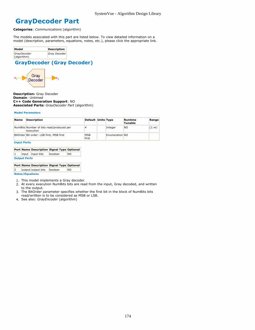
SystemVue - Algorithm Design Library
174
GrayDecoder PartCategories: Communications (algorithm)
The models associated with this part are listed below. To view detailed information on amodel (description, parameters, equations, notes, etc.), please click the appropriate link.
Model Description
GrayDecoder(algorithm)
Gray Decoder
GrayDecoder (Gray Decoder)
Description: Gray DecoderDomain: UntimedC++ Code Generation Support: NOAssociated Parts: GrayDecoder Part (algorithm)
Model Parameters
Name Description Default Units Type RuntimeTunable
Range
NumBits Number of bits read/produced perexecution
4 Integer NO [1:∞)
BitOrder Bit order: LSB first, MSB first MSBfirst
Enumeration NO
Input Ports
Port Name Description Signal Type Optional
1 input input bits boolean NO
Output Ports
Port Name Description Signal Type Optional
2 output output bits boolean NO
Notes/Equations
This model implements a Gray decoder.1.At every execution NumBits bits are read from the input, Gray decoded, and written2.to the output.The BitOrder parameter specifies whether the first bit in the block of NumBits bits3.read/written is to be considered as MSB or LSB.See also: GrayEncoder (algorithm)4.

SystemVue - Algorithm Design Library
175
GrayEncoder PartCategories: Communications (algorithm)
The models associated with this part are listed below. To view detailed information on amodel (description, parameters, equations, notes, etc.), please click the appropriate link.
Model Description
GrayEncoder(algorithm)
Gray Encoder
GrayEncoder (Gray Encoder)
Description: Gray EncoderDomain: UntimedC++ Code Generation Support: NOAssociated Parts: GrayEncoder Part (algorithm)
Model Parameters
Name Description Default Units Type RuntimeTunable
Range
NumBits Number of bits read/produced perexecution
4 Integer NO [1:∞)
BitOrder Bit order: LSB first, MSB first MSBfirst
Enumeration NO
Input Ports
Port Name Description Signal Type Optional
1 input input bits boolean NO
Output Ports
Port Name Description Signal Type Optional
2 output output bits boolean NO
Notes/Equations
This model implements a Gray encoder.1.At every execution NumBits bits are read from the input, Gray encoded, and written2.to the output.The BitOrder parameter specifies whether the first bit in the block of NumBits bits3.read/written is to be considered as MSB or LSB.Gray encoding maps natural binary numbers to a set of binary codes where two4.successive codes differ only in one bit.1-bit binary numbers and their Gray codesBinary Number Gray Code
0 0
1 1
2-bit binary numbers and their Gray codes (MSBs are to the left and LSBs to theright)
Binary Number Gray Code
00 00
01 01
10 11
11 10
3-bit binary numbers and their Gray codes (MSBs are to the left and LSBs to theright)
Binary Number Gray Code
000 000
001 001
010 011
011 010
100 110
101 111
110 101
111 100

SystemVue - Algorithm Design Library
176
4-bit binary numbers and their Gray codes (MSBs are to the left and LSBs to theright)
Binary Number Gray Code
0000 0000
0001 0001
0010 0011
0011 0010
0100 0110
0101 0111
0110 0101
0111 0100
1000 1100
1001 1101
1010 1111
1011 1110
1100 1010
1101 1011
1110 1001
1111 1000
The easiest way to construct a (N+1)-bit Gray code is to start with the N-bit Graycode, reflect it, then prepend the top half with 0 and the bottom half with 1.Following is an example showing how the 3-bit Gray code is constructed from the 2-bit Gray code.
Start with 2-bit Gray code00011110Reflect00011110---10110100Prepend 0 for the top half and 1 for the bottom half000001011010----110111101100
Gray encoding is commonly used in communications systems when mapping bits to5.constellation points so that adjacent constellation points are assigned bit patternsthat differ only in one bit. This helps minimize Bit Error Rate since in most caseserrors occur between adjacent constellation points and in this case only one bit willbe in error.See also: GrayDecoder (algorithm)6.

SystemVue - Algorithm Design Library
177
InterleaveDeinterleave PartCategories: Communications (algorithm)
The models associated with this part are listed below. To view detailed information on amodel (description, parameters, equations, notes, etc.), please click the appropriate link.
Model Description
InterleaveDeinterleave(algorithm)
Interleaver / Deinterleaver
InterleaveDeinterleave (Interleaver/Deinterleaver)
Description: Interleaver / DeinterleaverDomain: UntimedC++ Code Generation Support: NOAssociated Parts: InterleaveDeinterleave Part (algorithm)
Model Parameters
Name Description Default Units Type RuntimeTunable
Range
Rows Number of rows of the interleave/deinterleavematrix
8 Integer NO (0:∞)
Columns Number of columns of the interleave/deinterleavematrix
8 Integer NO (0:∞)
Input Ports
Port Name Signal Type Optional
1 input anytype NO
Output Ports
Port Name Signal Type Optional
2 output anytype NO
Notes/Equations
This component is a general purpose interleaver/de-interleaver. Every time it fires it1.reads (Rows × Columns) samples from its input and writes them to its output in adifferent order. Its operation is equivalent to writing the samples read from its inputin a Rows × Columns matrix row-wise, then reading the matrix elements column-wise and writing them to the output.Alternatively, the Transpose (algorithm) component in the Numeric Control librarycan be used.
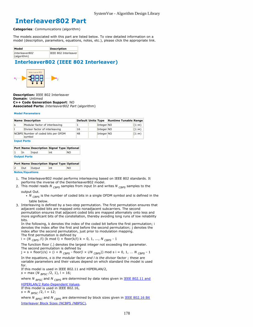
SystemVue - Algorithm Design Library
178
Interleaver802 PartCategories: Communications (algorithm)
The models associated with this part are listed below. To view detailed information on amodel (description, parameters, equations, notes, etc.), please click the appropriate link.
Model Description
Interleaver802(algorithm)
IEEE 802 Interleaver
Interleaver802 (IEEE 802 Interleaver)
Description: IEEE 802 InterleaverDomain: UntimedC++ Code Generation Support: NOAssociated Parts: Interleaver802 Part (algorithm)
Model Parameters
Name Description Default Units Type Runtime Tunable Range
s Modular factor of interleaving 1 Integer NO [1:∞)
l Divisor factor of interleaving 16 Integer NO [1:∞)
NCBPS Number of coded bits per OFDMsymbol
48 Integer NO [1:∞)
Input Ports
Port Name Description Signal Type Optional
1 In Input int NO
Output Ports
Port Name Description Signal Type Optional
2 Out Output int NO
Notes/Equations
The Interleaver802 model performs interleaving based on IEEE 802 standards. It1.performs the inverse of the Deinterleaver802 model.This model reads N CBPS samples from input In and writes N CBPS samples to the2.
output Out.N CBPS is the number of coded bits in a single OFDM symbol and is defined in the
table below.Interleaving is defined by a two-step permutation. The first permutation ensures that3.adjacent coded bits are mapped onto nonadjacent subcarriers. The secondpermutation ensures that adjacent coded bits are mapped alternately onto less andmore significant bits of the constellation, thereby avoiding long runs of low reliabilitybits.In the following, k denotes the index of the coded bit before the first permutation; idenotes the index after the first and before the second permutation; j denotes theindex after the second permutation, just prior to modulation mapping.The first permutation is defined byi = (N CBPS /l) (k mod l) + floor(k/l) k = 0, 1, ..., N CBPS - 1
The function floor (.) denotes the largest integer not exceeding the parameter.The second permutation is defined byj = s × floor(i/s) + (i + N CBPS - floor(l × i/N CBPS)) mod s i = 0, 1, ... N CBPS - 1
In the equations, s is the modular factor and l is the divisor factor ; these arevariable parameters and their values depend on which standard the model is usedfor.If this model is used in IEEE 802.11 and HIPERLAN/2,s = max (N BPSC /2, 1), l = 16;
where N BPSC and N CBPS are determined by data rates given in IEEE 802.11 and
HIPERLAN/2 Rate-Dependent Values.If this model is used in IEEE 802.16,s = N BPSC /2, l = 12;
where N BPSC and N CBPS are determined by block sizes given in IEEE 802.16 Bit
Interleaver Block Sizes (NCBPS /NBPSC).

SystemVue - Algorithm Design Library
179
IEEE 802.11 and HIPERLAN/2 Rate-Dependent Values
Data Rate(Mbps)
Modulation CodingRate (R)
Coded Bits perSubcarrier(NBPSC)
Coded Bits perOFDM Symbol(NCBPS)
Data Bits perOFDM Symbol(NDBPS)
6 BPSK 1/2 1 48 24
9 BPSK 3/4 1 48 36
12 QPSK 1/2 2 96 48
18 QPSK 3/4 2 96 72
24 (IEEE802.11a)
16QAM 1/2 4 192 96
27(HIPERLAN/2)
16QAM 9/16 4 192 108
36 16QAM 3/4 4 192 144
48 (IEEE802.11a)
64QAM 2/3 6 288 192
54 64QAM 3/4 6 288 216
IEEE 802.16 Bit Interleaver Block Sizes (N CBPS /N BPSC)
Modulation 16 Subchannels(Default)
8Subchannels
4Subchannels
2Subchannels
1Subchannel
QPSK 384/2 192/2 96/2 48/2 24/2
16QAM 768/4 384/4 192/4 96/4 48/4
64QAM 1152/6 576/6 288/6 144/6 72/6
See Also:
Deinterleaver802 (algorithm)
References
IEEE Standard 802.11a-1999, Part 11: Wireless LAN Medium Access Control (MAC)1.and Physical Layer (PHY) specifications: High-speed Physical Layer in the 5 GHzBand, 1999.ETSI TS 101 475 v1.1.1, Broadband Radio Access Networks (BRAN); HIPERLAN Type2.2; Physical (PHY) layer, April, 2000.IEEE P802.16-REVd/D2-2003, Part 16 Air Interface for Fixed Broadcast Wireless3.Access Systems.

SystemVue - Algorithm Design Library
180
LFSR PartCategories: C++ Code Generation (algorithm), Communications (algorithm)
The models associated with this part are listed below. To view detailed information on amodel (description, parameters, equations, notes, etc.), please click the appropriate link.
Model Description
LFSR(algorithm)
Linear Feedback Shift Register
LFSR
Description: Linear Feedback Shift RegisterDomain: UntimedC++ Code Generation Support: YESAssociated Parts: LFSR Part (algorithm)
Model Parameters
Name Description Default Units Type Runtime Tunable
FeedbackTaps Feedback tap positions [3, 10] None NO
InitialState Initial state non-zero bit positions [5, 9] None NO
UseInternalReset Internal periodic reset mode: NO,YES
NO Enumeration NO
InternalResetPeriod Number of outputs in a period 127 Integer NO
Input Ports
Port Name Signal Type Optional
1 clock int NO
2 reset int YES
Output Ports
Port Name Signal Type Optional
3 output multiple int NO
Notes/Equations
The linear feedback shift register (LFSR) part is configured to generate a PN1.sequence.For every clock input, there is an LFSR output.2.The output may be connected to a bus which can make all LFSR bits observable. A3.non-bus connection permit the standard output which is the rightmost bit in the LFSRModel. For a bus labeled B(a:b), B(a) is the standard output connection. If a<b,B(a+1) is the adjacent bit to the standard output and so on. This default connectionorder can be changed. Consult Nets Connection Lines and Buses (users). Note thatany bus width specification greater than the LFSR number of bits generates an error.New bit values are generated when the clock input is true (not 0) and the reset input4.is false (0), if the reset input is connected. Otherwise, the previous bit value isoutput.When the reset input is true (not 0), the bits of InitialState is available for output.5.If UseInternalReset is YES, then any reset input is ignored. The LFSR starts from6.InitialState every InternalResetPeriod samples.The parameters FeedbackTaps and InitialState permit configuration for a LFSR with7.length up to 64 bits.Both parameters can be specified either as a bit array or as an array of positions8.having bit value 1. The implied length of the bit array notation is the number of arrayelements. For the positional notation, the implied length is the largest position value.The LFSR length r is defined by the implied length of FeedbackTaps. For example, if9.FeedbackTaps is specified as [7 3 2 1] in the positional notation or equivalently [1 11 0 0 0 1] in the bit array notation, then the LFSR length is 7 bits.The diagram below illustrates the LFSR model.10.
LFSR Model
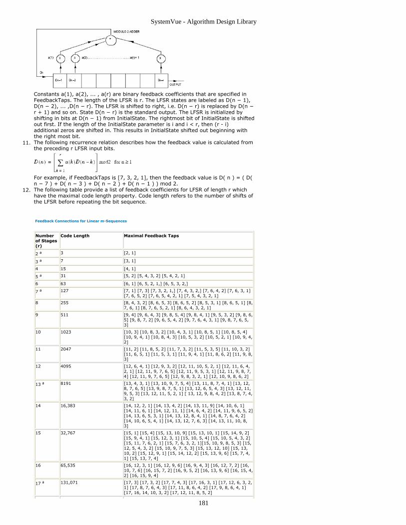
SystemVue - Algorithm Design Library
181
Constants a(1), a(2), ... , a(r) are binary feedback coefficients that are specified inFeedbackTaps. The length of the LFSR is r. The LFSR states are labeled as D(n − 1),D(n − 2), ... ,D(n − r). The LFSR is shifted to right, i.e. D(n − r) is replaced by D(n −r + 1) and so on. State D(n − r) is the standard output. The LFSR is initialized byshifting in bits at D(n − 1) from InitialState. The rightmost bit of InitialState is shiftedout first. If the length of the InitialState parameter is i and i < r, then (r - i)additional zeros are shifted in. This results in InitialState shifted out beginning withthe right most bit.The following recurrence relation describes how the feedback value is calculated from11.the preceding r LFSR input bits.
For example, if FeedbackTaps is [7, 3, 2, 1], then the feedback value is D( n ) = ( D(n − 7 ) + D( n − 3 ) + D( n − 2 ) + D( n − 1 ) ) mod 2.The following table provide a list of feedback coefficients for LFSR of length r which12.have the maximal code length property. Code length refers to the number of shifts ofthe LFSR before repeating the bit sequence.
Feedback Connections for Linear m-Sequences
Numberof Stages(r)
Code Length Maximal Feedback Taps
2 a 3 [2, 1]
3 a 7 [3, 1]
4 15 [4, 1]
5 a 31 [5, 2] [5, 4, 3, 2] [5, 4, 2, 1]
6 63 [6, 1] [6, 5, 2, 1,] [6, 5, 3, 2,]
7 a 127 [7, 1] [7, 3] [7, 3, 2, 1,] [7, 4, 3, 2,] [7, 6, 4, 2] [7, 6, 3, 1][7, 6, 5, 2] [7, 6, 5, 4, 2, 1] [7, 5, 4, 3, 2, 1]
8 255 [8, 4, 3, 2] [8, 6, 5, 3] [8, 6, 5, 2] [8, 5, 3, 1] [8, 6, 5, 1] [8,7, 6, 1] [8, 7, 6, 5, 2, 1] [8, 6, 4, 3, 2, 1]
9 511 [9, 4] [9, 6, 4, 3] [9, 8, 5, 4] [9, 8, 4, 1] [9, 5, 3, 2] [9, 8, 6,5] [9, 8, 7, 2] [9, 6, 5, 4, 2] [9, 7, 6, 4, 3, 1] [9, 8, 7, 6, 5,3]
10 1023 [10, 3] [10, 8, 3, 2] [10, 4, 3, 1] [10, 8, 5, 1] [10, 8, 5, 4][10, 9, 4, 1] [10, 8, 4, 3] [10, 5, 3, 2] [10, 5, 2, 1] [10, 9, 4,2]
11 2047 [11, 2] [11, 8, 5, 2] [11, 7, 3, 2] [11, 5, 3, 5] [11, 10, 3, 2][11, 6, 5, 1] [11, 5, 3, 1] [11, 9, 4, 1] [11, 8, 6, 2] [11, 9, 8,3]
12 4095 [12, 6, 4, 1] [12, 9, 3, 2] [12, 11, 10, 5, 2, 1] [12, 11, 6, 4,2, 1] [12, 11, 9, 7, 6, 5] [12, 11, 9, 5, 3, 1] [12, 11, 9, 8, 7,4] [12, 11, 9, 7, 6, 5] [12, 9, 8, 3, 2, 1] [12, 10, 9, 8, 6, 2]
13 a 8191 [13, 4, 3, 1] [13, 10, 9, 7, 5, 4] [13, 11, 8, 7, 4, 1] [13, 12,8, 7, 6, 5] [13, 9, 8, 7, 5, 1] [13, 12, 6, 5, 4, 3] [13, 12, 11,9, 5, 3] [13, 12, 11, 5, 2, 1] [ 13, 12, 9, 8, 4, 2] [13, 8, 7, 4,3, 2]
14 16,383 [14, 12, 2, 1] [14, 13, 4, 2] [14, 13, 11, 9] [14, 10, 6, 1][14, 11, 6, 1] [14, 12, 11, 1] [14, 6, 4, 2] [14, 11, 9, 6, 5, 2][14, 13, 6, 5, 3, 1] [14, 13, 12, 8, 4, 1] [14, 8, 7, 6, 4, 2][14, 10, 6, 5, 4, 1] [14, 13, 12, 7, 6, 3] [14, 13, 11, 10, 8,3]
15 32,767 [15, 1] [15, 4] [15, 13, 10, 9] [15, 13, 10, 1] [15, 14, 9, 2][15, 9, 4, 1] [15, 12, 3, 1] [15, 10, 5, 4] [15, 10, 5, 4, 3, 2][15, 11, 7, 6, 2, 1] [15, 7, 6, 3, 2, 1][15, 10, 9, 8, 5, 3] [15,12, 5, 4, 3, 2] [15, 10, 9, 7, 5, 3] [15, 13, 12, 10] [15, 13,10, 2] [15, 12, 9, 1] [15, 14, 12, 2] [15, 13, 9, 6] [15, 7, 4,1] [15, 13, 7, 4]
16 65,535 [16, 12, 3, 1] [16, 12, 9, 6] [16, 9, 4, 3] [16, 12, 7, 2] [16,10, 7, 6] [16, 15, 7, 2] [16, 9, 5, 2] [16, 13, 9, 6] [16, 15, 4,2] [16, 15, 9, 4]
17 a 131,071 [17, 3] [17, 3, 2] [17, 7, 4, 3] [17, 16, 3, 1] [17, 12, 6, 3, 2,1] [17, 8, 7, 6, 4, 3] [17, 11, 8, 6, 4, 2] [17, 9, 8, 6, 4, 1][17, 16, 14, 10, 3, 2] [17, 12, 11, 8, 5, 2]
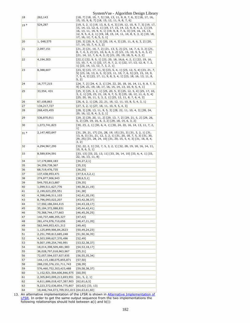
SystemVue - Algorithm Design Library
182
18 262,143 [18, 7] [18, 10, 7, 5] [18, 13, 11, 9, 8, 7, 6, 3] [18, 17, 16,15, 10, 9, 8, 7] [18, 15, 12, 11, 9, 8, 7, 6]
19 a 524,287 [19, 5, 2, 1] [19, 13, 8, 5, 4, 3] [19, 12, 10, 9, 7, 3] [19, 17,15, 14, 13, 12, 6, 1] [19, 17, 15, 14, 13, 9, 8, 4, 2, 1] [19,16, 13, 11, 19, 9, 4, 1] [19, 9, 8, 7, 6, 3] [19, 16, 15, 13,12, 9, 5, 4, 2, 1] [19, 18, 15, 14, 11, 10, 8, 5, 3, 2] [19, 18,17, 16, 12, 7, 6, 5, 3, 1]
20 1, 048,575 [20, 3] [20, 9, 5, 3] [20, 19, 4, 3] [20, 11, 8, 6, 3, 2] [20,17, 14, 10, 7, 4, 3, 2]
21 2,097,151 [21, 2] [21, 14, 7, 2] [21, 13, 5, 2] [21, 14, 7, 6, 3, 2] [21,8, 7, 4, 3, 2] [21, 10, 6, 4, 3, 2] [21, 15, 10, 9, 5, 4, 3, 2][21, 14, 12, 7, 6, 4, 3, 2] [21, 20, 19, 18, 5, 4, 3, 2]
22 4,194,303 [22,1] [22, 9, 5, 1] [22, 20, 18, 16,6, 4, 2, 1] [22, 19, 16,13, 10, 7, 4, 1] [22, 17, 9, 7, 2, 1] [22, 17, 13, 12, 8, 7, 2,1] [22, 14, 13, 12, 7, 3, 2, 1]
23 8,388,607 [23, 5] [23, 17, 11, 5] [23, 5, 4, 1] [23, 12, 5, 4] [23, 21, 7,5] [23, 16, 13, 6, 5, 3] [23, 11, 10, 7, 6, 5] [23, 15, 10, 9,7, 5, 4, 3] [23, 17, 11, 9, 8, 5, 4, 1] [23, 18, 16, 13, 11, 8,5, 2]
24 16,777,215 [24, 7, 2] [24, 4, 3, 1] [24, 22, 20, 18, 16, 14, 11, 9, 8, 7, 5,4] [24, 21, 19, 18, 17, 16, 15, 14, 13, 10, 9, 5, 4, 1]
25 33,554, 431 [25, 3] [25, 3, 2, 1] [25, 20, 5, 3] [25, 12, 5, 4] [25, 17, 10,3, 2, 1] [25, 23, 21, 19, 9, 7, 5, 3] [25, 18, 12, 11, 6, 5, 4][25, 20, 16, 11, 5, 3, 2, 1] [25, 12, 11, 8, 7, 6, 4, 3]
26 67,108,863 [26, 6, 2, 1] [26, 22, 21, 16, 12, 11, 10, 8, 5, 4, 3, 1]
27 134,217,727 [27, 5, 2, 1] [27, 18, 11, 10, 9, 5, 4, 3]
28 268,435,455 [28, 3] [28, 13, 11, 9, 5, 3] [28, 22, 11, 10, 4, 3] [28, 24,20, 16, 12, 8, 4, 3, 2, 1]
29 536,870,911 [29, 2] [29, 20, 11, 2] [29, 13, 7, 2] [29, 21, 5, 2] [29, 26,5, 2] [29, 19, 16, 6, 3, 2] [29, 18, 14, 6, 3, 2]
30 1,073,741,823 [30, 23, 2, 1] [30, 6, 4, 1] [30, 24, 20, 16, 14, 13, 11, 7, 2,1]
31 a 2,147,483,647 [31, 29, 21, 17] [31, 28, 19, 15] [31, 3] [31, 3, 2, 1] [31,13, 8, 3] [31, 21, 12, 3, 2, 1] [31, 20, 18, 7, 5, 3] [31, 30,29, 25] [31, 28, 24, 10] [31, 20, 15, 5, 4, 3] [31, 16, 8, 4,3, 2]
32 4,294,967,295 [32, 22, 2, 1] [32, 7, 5, 3, 2, 1] [32, 28, 19, 18, 16, 14, 11,10, 9, 6, 5, 1]
33 8,589,934,591 [33, 13] [33, 22, 13, 11] [33, 26, 14, 10] [33, 6, 4, 1] [33,22, 16, 13, 11, 8]
34 17,179,869,183 [34,27,2,1]
35 34,359,738,367 [35,33]
36 68,719,476,735 [36,25]
37 137,438,953,471 [37,5,4,3,2,1]
38 274,877,906,943 [38,6,5,1]
39 549,755,813,887 [39,35]
40 1,099,511,627,776 [40,38,21,19]
41 2,199,023,255,551 [41,38]
42 4,398,046,511,103 [42,41,20,19]
43 8,796,093,022,207 [43,42,38,37]
44 17,592,186,044,415 [44,43,18,17]
45 35,184,372,088,831 [45,44,42,41]
46 70,368,744,177,663 [46,45,26,25]
47 140,737,488,355,327 [47,42]
48 281,474,976,710,656 [48,47,21,20]
49 562,949,953,421,312 [49,40]
50 1,125,899,906,84,2623 [50,49,24,23]
51 2,251,799,813,685,248 [51,50,36,35]
52 4,503,599,627,370,496 [52,49]
53 9,007,199,254,740,991 [53,52,38,37]
54 18,014,398,509,481,983 [54,53,18,17]
55 36,028,797,018,963,967 [55,31]
56 72,057,594,037,927,935 [56,55,35,34]
57 144,115,188,075,855,871 [57,50]
58 288,230,376,151,711,743 [58,39]
59 576,460,752,303,423,488 [59,58,38,37]
60 1,152,921,504,606,846,975 [60,59]
61 2,305,843,009,213,693,951 [61, 5, 2, 1]
62 4,611,686,018,427,387,903 [62,61,6,5]
63 9,223,372,036,854,775,807 [63,62] [33, 13]
64 18,446,744,073,709,551,615 [64,63,61,60]
An alternative implementation of the LFSR is shown in Alternative Implementation of13.LFSR. In order to get the same output sequence from the two implementations thefollowing relationships should hold between a(i) and b(i):
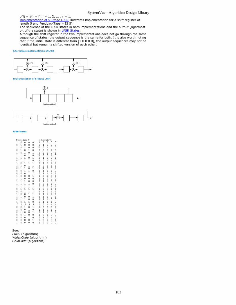
SystemVue - Algorithm Design Library
183
b(i) = a(r − i), i = 1, 2, ... , r − 1.Implementation of 5-Stage LFSR illustrates implementation for a shift register oflength 5 and FeedbackTaps = [2 5].The sequence of the LFSR states in both implementations and the output (rightmostbit of the state) is shown in LFSR States.Although the shift register in the two implementations does not go through the samesequence of states, the output sequence is the same for both. It is also worth notingthat if the initial state is different from [1 0 0 0 0], the output sequences may not beidentical but remain a shifted version of each other.
Alternative Implementation of LFSR
Implementation of 5-Stage LFSR
LFSR States
See:PRBS (algorithm)WalshCode (algorithm)GoldCode (algorithm)

SystemVue - Algorithm Design Library
184
LoadIFFTBuff802 PartCategories: C++ Code Generation (algorithm), Communications (algorithm)
The models associated with this part are listed below. To view detailed information on amodel (description, parameters, equations, notes, etc.), please click the appropriate link.
Model Description
LoadIFFTBuff802(algorithm)
IEEE 802 IFFT Buffer Loader
LoadIFFTBuff802 (IEEE 802 IFFT Buffer Loader)
Description: IEEE 802 IFFT Buffer LoaderDomain: UntimedC++ Code Generation Support: YESAssociated Parts: LoadIFFTBuff802 Part (algorithm)
Model Parameters
Name Description Default Units Type RuntimeTunable
Carriers Number of subcarriers per OFDMsymbol
52 Integer NO
DCCarrier DC carrier: OFF, ON OFF Enumeration NO
DCPilotValue DC Pilot Value 1.33333 Complexnumber
YES
FullSubcarriers Activate all sub-carriers: NO, YES YES Enumeration NO
SubcarrierList Subcarrier list [-21, -7, 7,21]
None NO
Order IFFT points as 2^Order 7 Integer NO
Input Ports
Port Name Description Signal Type Optional
1 In Transmitted signal before IFFT complex NO
Output Ports
Port Name Description Signal Type Optional
2 Out IFFT input signal, zero padded complex NO
Notes/Equations
This component is used to load transmission data into the IFFT buffer. Each firing,1.Carriers tokens are consumed and 2 Order tokens are generated. For example, ifCarriers = 52, Order = 7, 52 tokens are consumed and 128 tokens are generated.Data loading is performed as follows.2.Assume x(0), x(1), ... , x(N-1) are the inputs that generally represent activesubcarriers defined by designers, where N = Carriers. y(0), y(1), ... , y(M-1) are theoutputs, M = 2 Order.when N is even
when N is odd
For example, if Order = 4 and Carriers = 7, the input carriers are x(0), x(1), x(2),x(3),x(4),x(5),x(6), and the output carrier sequence would be:0 , x(3) , x(4) , x(5) , x(6) , 0 , 0 , 0 , 0 , 0 , 0 , 0 , 0 , x(0) , x(1) , x(2)which will be loaded into the IFFT model for the IFFT transformation.

SystemVue - Algorithm Design Library
185
DCCarrier and DCPilotValue specify whether DC carrier is used; if DCCarrier = ON,3.the DC carrier value is set by DCPilotValue.In the example provided in note 2, DCCarrier = OFF.While DCCarrier = ON and DCPilotValue = 4/3, the output carriers sequence wouldbe:4/3, x(3), x(4), x(5), x(6), 0, 0, 0, 0, 0, 0, 0, 0, x(0), x(1), x(2)in which the first carrier is 4/3 instead of 0.If FullSubcarriers = YES, all input carriers will be used. If FullSubcarriers = NO, some4.of the input carriers will be used; SubcarrierList specifies which input carriers will beused.SubcarrierList (valid when FullSubcarriers = NO) specifies the positions of the input5.carriers to be used as active subcarriers (all subcarriers are 0 except those carriersspecified).Assume x(0), x(1), ... , x(N-1) are the input signals that generally represent activesubcarriers defined by designers, where N = Carriers. y(0), y(1), ... , y(M-1) are theoutput of the model M = 2 Order. The corresponding indices of x(0), x(1), ... , x(N-1)are {int(-Carriers/2), int(-Carriers/2) + 1, ... , -1, 1, ... , int(Carriers/2)-1,int(Carriers/2)}.The active subcarrier loading procedure is performed as follows: assume index is anelement of {int(-Carriers/2), int(-Carriers/2) + 1, ... , -1, 1, ... , int(Carriers/2)-1,int(Carriers/2)}:when N is even
when N is odd
For example, SubcarrierList = {-2, -1, 2, 3}, and input carriers are x(0), x(1), x(2),x(3), x(4), x(5), x(6). Indices of the input carriers are -3, -2, -1, 1, 2, 3, 4.Elements in SubcarrierList must be integer and in (-Carriers/2, Carriers/2), in whichCarriers is the number of carriers of input, here, it is 7 and index should be in [-3, 3].In this case, the carrier with index is -2, -1, 2, 3 is used, these are x(1), x(2), x(4),x(5). The output subcarriers are then:4/3, 0, x(4), x(5), 0, 0, 0, 0, 0, 0, 0, 0, 0, 0, x(1), x(2).
References
IEEE Standard 802.11a-1999, "Part 11: Wireless LAN Medium Access Control (MAC)1.and Physical Layer (PHY) specifications: High-speed Physical Layer in the 5 GHzBand," 1999.ETSI TS 101 475 v1.1.1, "Broadband Radio Access Networks (BRAN); HIPERLAN Type2.2; Physical (PHY) layer," April, 2000.ARIB-JAPAN, Terrestrial Integrated Services Digital Broadcasting (ISDB-T);3.Specification of Channel Coding, Frame Structure and Modulation, Sept.1998.ETSI, Digital Video Broadcasting (DVB); Framing structure, channel coding and4.modulation for digital terrestrial television. EN300 744 v1.2.1, EuropeanTelecommunication Standard, July 1999.IEEE P802.15-03/268r1, "Multi-band OFDM Physical Layer Proposal for IEEE 802.155.Task Group 3a," September 2003.IEEE P802.16-REVd/D2-2003, "Draft IEEE Standard for Local and metropolitan area6.networks Part 16: Air Interface for Fixed Broadband Wireless Access Systems," 2003.

SystemVue - Algorithm Design Library
186
Modulator PartCategories: Analog/RF (algorithm), Communications (algorithm)
The models associated with this part are listed below. To view detailed information on amodel (description, parameters, equations, notes, etc.), please click the appropriate link.
Model Description
Modulator(algorithm)
Modulator
Modulator (Modulator)
Description: ModulatorDomain: TimedC++ Code Generation Support: NOAssociated Parts: Modulator Part (algorithm)
Model Parameters
Name Description Default Units Type RuntimeTunable
Range Symbol
InputType Input type: I/Q,Amp/Phase, Amp/Freq
I/Q Enumeration NO
FCarrier Carrier frequency (used ifoptional LO input notused)
0.2e6 Hz Float NO [0:∞) fc
InitialPhase Initial phase 0 deg Float NO (-∞:∞)
θ
AmpSensitivity Amplitude sensitivity 1 Float NO (-∞:∞)
Sa
PhaseSensitivity Phase deviation sensitivityin degrees/Volt
90 Float NO (-∞:∞)
Sp
FreqSensitivity Frequency deviationsensitivity in Hz/Volt
10000 Float NO (-∞:∞)
Sf
ConjugatedQuadrature Negate quadrature output:NO, YES
NO Enumeration NO
MirrorSignal Mirror signal about carrier:NO, YES
NO Enumeration NO
ShowIQ_Impairments Show I and Qimpairments: NO, YES
NO Enumeration NO
GainImbalance Gain imbalance in dB 0.0 Float NO (-∞:∞)
G
PhaseImbalance Phase imbalance 0.0 deg Float NO (-∞:∞)
φ
I_OriginOffset I origin offset 0.0 Float NO (-∞:∞)
Ioff
Q_OriginOffset Q origin offset 0.0 Float NO (-∞:∞)
Qoff
IQ_Rotation IQ rotation 0.0 deg Float NO (-∞:∞)
R
Input Ports
Port Name Description Signal Type Optional
1 input1 input1 real YES
2 input2 input2 real YES
3 LO complex envelope local oscillator signal envelope YES
Output Ports
Port Name Description Signal Type Optional
4 output complex envelope vector output envelope NO
5 quad_output complex envelope vector quadratureoutput
envelope NO
Notes/Equations

SystemVue - Algorithm Design Library
187
The Modulator model implements a modulator that can perform amplitude, phase,1.frequency, or I/Q modulation.This model reads one sample from its inputs and writes one sample to its outputs.2.The LO input is optional. When not connected, an internal LO signal is used at the3.frequency FCarrier. When the external LO input is used, it must be a complexenvelope signal with characterization frequency greater than zero. If use with a realsignal is needed, then the LO input to this model can be preceded with anEnvFcChange (algorithm) model that will recharacterize a real signal to itsrepresentation at a specified frequency. The LO input can include power, phase, andnoise variations in the LO signal. In the following, fc is used to refer to the FCarrier
parameter (when there is no LO input) or to the characterization frequency of thesignal at the LO input.When fc > 0, the outputs are complex envelope signals with characterization4.
frequency equal to fc. The output is a complex value of the form I + j·Q.
When fc = 0, the outputs are real baseband signals.5.
Basic operation for generating the modulated complex envelope signal (cx)6.When InputType is set to I/Q, this model acts as an I/Q modulator. The I signalis applied at input1 while the Q signal is applied at input2. The output signal isgiven bycx = Sa·(input1 + j·input2)
Either input (but not both) can be left disconnected, in which case its value isassumed to be 0.When InputType is set to Amp/Phase, this model acts as an amplitude andphase modulator. The amplitude modulating signal is applied at input1, and thephase modulating signal is applied at input2. The output signal is given bycx = Sa·input1·ej·(input2·S
p·π / 180 + θ)
Either input (but not both) can be left disconnected.If input1 is left disconnected, then its value is assumed to be 1 and Sa is set to
1. In this case, this model acts as a pure phase modulator.If input2 is left disconnected, then its value is assumed to be 0. In this case, thismodel acts as a pure amplitude modulator.When InputType is set to Amp/Freq, this model acts as an amplitude andfrequency modulator. The amplitude modulating signal is applied at input1, andthe frequency modulating signal is applied at input2. The output signal is givenby
Either input (but not both) can be left disconnected.If input1 is left disconnected, then its value is assumed to be 1 and Sa is set to
1. In this case, this model acts as a pure frequency modulator.If input2 is left disconnected, then its value is assumed to be 0. In this case, thismodel acts as a pure amplitude modulator.
Effect of MirrorSignal on the modulated complex envelope signal (cx)7.If MirrorSignal = YES, then let cx = conjugate( cx)
Effect of GainImbalance, PhaseImbalance, I_OriginOffset, Q_OriginOffset, and8.IQ_Rotation on the modulated complex envelope signal (cx)Assuming that cx is of the form I(t) + j·Q(t), then the real signal that this complexenvelope signal represents is I(t)·cos( 2πfct ) − Q(t)·sin( 2πfct ).
When there is GainImbalance and PhaseImbalance, the local oscillator signalsfor the in-phase and quadrature phase mixers are not cos( 2πfct ) and sin( 2πfct
) butLOI = gI · cos( 2πfct + φI )
LOQ = gQ · sin( 2πfct + φQ )
where gI, gQ, φI, φQ are the gain and phase imbalances. This model uses a
symmetric implementation of the imbalances wheregI = 100.5·G/20
gQ = 10−0.5·G/20
φI = −φ/2
φQ = φ/2
When these imbalances are taken into account the output signal isI(t) · gI · cos( 2πfct + φI ) − Q(t) · gQ · sin( 2πfct + φQ ) =
I(t) · gI · [ cos( 2πfct ) · cos( φI ) − sin( 2πfct ) · sin( φI ) ] − Q(t) · gQ · [ sin(
2πfct ) · cos( φQ ) + cos( 2πfct ) · sin( φQ ) ] =
[ gI · I(t) · cos( φI ) − gQ · Q(t) · sin( φQ ) ] · cos( 2πfct ) − [ gI · I(t) · sin( φI )
+ gQ · Q(t) · cos( φQ ) ] · sin( 2πfct ) =
I'(t) · cos( 2πfct ) − Q'(t) · sin( 2πfct )

SystemVue - Algorithm Design Library
188
whereI'(t) = gI · I(t) · cos( φI ) − gQ · Q(t) · sin( φQ )
Q'(t) = gI · I(t) · sin( φI ) + gQ · Q(t) · cos( φQ )
For IQ_Rotation, cx = cx·( cos(R)+j·sin(R) )For I_OriginOffset and Q_OriginOffset, cx = cx + (Ioff + j·Qoff)
Obtaining the output and quad_output signals from the modulated complex envelope9.signal cx = Re{cx} + j·Im{cx}
When fc > 0, output = cx and quad_output = −Im{cx} + j·Re{cx}
When fc = 0, output = Re{cx} and quad_output = Im{cx}
See also: Demodulator (algorithm)10.
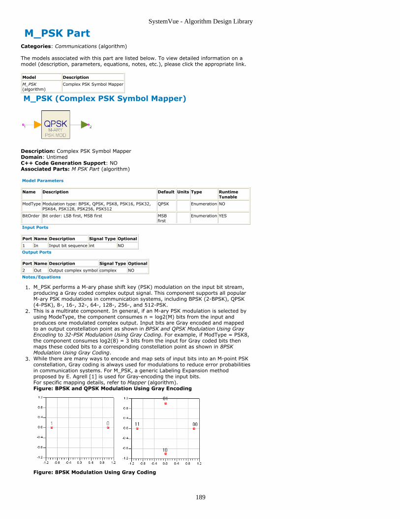
SystemVue - Algorithm Design Library
189
M_PSK PartCategories: Communications (algorithm)
The models associated with this part are listed below. To view detailed information on amodel (description, parameters, equations, notes, etc.), please click the appropriate link.
Model Description
M_PSK(algorithm)
Complex PSK Symbol Mapper
M_PSK (Complex PSK Symbol Mapper)
Description: Complex PSK Symbol MapperDomain: UntimedC++ Code Generation Support: NOAssociated Parts: M PSK Part (algorithm)
Model Parameters
Name Description Default Units Type RuntimeTunable
ModType Modulation type: BPSK, QPSK, PSK8, PSK16, PSK32,PSK64, PSK128, PSK256, PSK512
QPSK Enumeration NO
BitOrder Bit order: LSB first, MSB first MSBfirst
Enumeration YES
Input Ports
Port Name Description Signal Type Optional
1 In Input bit sequence int NO
Output Ports
Port Name Description Signal Type Optional
2 Out Output complex symbol complex NO
Notes/Equations
M_PSK performs a M-ary phase shift key (PSK) modulation on the input bit stream,1.producing a Gray coded complex output signal. This component supports all popularM-ary PSK modulations in communication systems, including BPSK (2-BPSK), QPSK(4-PSK), 8-, 16-, 32-, 64-, 128-, 256-, and 512-PSK.This is a multirate component. In general, if an M-ary PSK modulation is selected by2.using ModeType, the component consumes n = log2(M) bits from the input andproduces one modulated complex output. Input bits are Gray encoded and mappedto an output constellation point as shown in BPSK and QPSK Modulation Using GrayEncoding to 32-PSK Modulation Using Gray Coding. For example, if ModType = PSK8,the component consumes log2(8) = 3 bits from the input for Gray coded bits thenmaps these coded bits to a corresponding constellation point as shown in 8PSKModulation Using Gray Coding.While there are many ways to encode and map sets of input bits into an M-point PSK3.constellation, Gray coding is always used for modulations to reduce error probabilitiesin communication systems. For M_PSK, a generic Labeling Expansion methodproposed by E. Agrell [1] is used for Gray-encoding the input bits.For specific mapping details, refer to Mapper (algorithm).Figure: BPSK and QPSK Modulation Using Gray Encoding
Figure: 8PSK Modulation Using Gray Coding

SystemVue - Algorithm Design Library
190
Figure: 16-PSK Modulation Using Gray Coding
Figure: 32-PSK Modulation Using Gray Coding

SystemVue - Algorithm Design Library
191
References
E. Agrell, J.Lassing, E. G. Strüm, and T. Ottosson, "On the optimality of the binary1.reflected Gray code," IEEE Transactions on Information Theory, vol. 50, no. 12, pp.3170-3182, Dec. 2004.M. Jeruchim, P. Balaban and K. Shanmugan, Simulation of Communication Systems,2.Plenum Press, New York and London, 1992.

SystemVue - Algorithm Design Library
192
MuxOFDMSym802 PartCategories: Communications (algorithm)
The models associated with this part are listed below. To view detailed information on amodel (description, parameters, equations, notes, etc.), please click the appropriate link.
Model Description
MuxOFDMSym802(algorithm)
IEEE 802 OFDM Symbol Multiplexer
MuxOFDMSym802 (IEEE 802 OFDM SymbolMultiplexer)
Description: IEEE 802 OFDM Symbol MultiplexerDomain: UntimedC++ Code Generation Support: NOAssociated Parts: MuxOFDMSym802 Part (algorithm)
Model Parameters
Name Description Default Units Type RuntimeTunable
Range
Carriers Number of subcarriers perOFDM symbol
52 Integer NO [1:8192]
DataCarriers Number of data subcarriersper OFDM symbol
48 Integer NO [1:8192]
PilotPosition Standard pilot positions [-21, -7, 7,21]
Integerarray
NO
PilotValue Standard pilot values [1, 1, 1, -1] Complexarray
NO
GuardCarrierPosition Guard carrier positions Integerarray
NO
GuardCarrierValue Guard carrier values Complexarray
NO
Input Ports
Port Name Description Signal Type Optional
1 Data data subcarriers input complex NO
2 Pilot continual pilot value complex NO
Output Ports
Port Name Description Signal Type Optional
3 Out OFDM symbol output complex NO
Notes/Equations
This component is used to multiplex data and pilot subcarriers into the OFDM symbol1.for IEEE 802 standards 802.11a, 802.11g, 802.15.3a, 802.16a, and 802.16d.
NoteOFDM symbols generally consist of continual pilots (CP) and scattered pilots (SP). Current IEEE 802standards use CP only. Even though some DAB, DVB-T, and ISDB-T OFDM systems may use both CPand SP, MuxOFDMSym802 supports CP only.
The basic OFDM symbol structure is introduced in the frequency domain. The symbol2.(illustrated in OFDM Symbol) consists of subcarriers that determine the size of theFFT. There are several subcarrier types:
Data subcarriers for data transmissionPilot subcarriers for estimationsNull subcarriers for no transmission, for guard bands and DC subcarrier.Guard bands in most OFDM systems (DVB-T, ISDB-T, 802.11a, 802.11g,802.16a, and 802.16d) are inserted zeros.IEEE 802.15.3a has additional guard carriers defined between data subcarriersand guard bands. The guard subcarriers can be used for various purposes,including relaxing the specification on transmit and receive filters. Themagnitude level of the guard tones is not specified, so reduced power levels forthese subcarriers can be used. The all-zeros guard bands allow the signal tonaturally decay and create the FFT brick wall shaping.

SystemVue - Algorithm Design Library
193
OFDM Symbol
This component multiplexes data and pilot subcarriers into one OFDM symbolaccording to the positions of data and pilot subcarriers defined in the standards.The null subcarriers (guard bands and DC subcarrier) are inserted into an OFDMsymbol by the LoadIFFTBuff802 component. (Both MuxOFDMSym802 andLoadIFFTBuff802 components implement an OFDM symbol in the frequencydomain.)
MuxOFDMSym802 parameter settings enable designers to generate a variety of3.OFDM symbol formats, in accordance with IEEE standards or not.Carriers specifies the number of active subcarriers (data subcarriers, pilot subcarriersand guard subcarriers) in one OFDM symbol.
NoteCarriers = DataCarriers _ PilotPosition _ GuardCarrierPosition.
DataCarriers specifies the number of data subcarriers in one OFDM symbol.PilotPosition specifies continual pilot positions; PilotPosition is the number of pilotsubcarriers in one OFDM symbol.PilotValue specifies values for continual pilot positions.GuardCarrierPosition specifies guard carriers positions (default = NULL);GuardCarrierPosition is the number of guard carrier subcarriers in one OFDM symbol.GuardCarrierValue specifies values for guard carrier positions (default = NULL).Each firing, one Pilot token and DataCarriers tokens are consumed and Carriers4.tokens are output.The complex Data input signal is directly multiplexed into the OFDM symbol.The continual pilots are multiplexed into OFDM symbols as follows:p k is the input in Pilot pin for kth OFDM symbol (or kth firing)
a 0, a 1, ... , a n are n+1 pilot values defined by PilotValue
The actual pilot values of kth OFDM symbol are p k × a 0, p k × a 1, ... , p k × a n.
The continual pilot subcarrier values are multiplexed into the OFDM symbol accordingto PilotPosition.The guard carriers are multiplexed into the OFDM symbol like continual pilot asfollows:b 0, b 1, ... , b m are m+1 guard carriers values specified by GuardCarrierValue.
The actual guard carrier values of kth OFDM symbol are p k × b 0, p k × b 1, ... , p k
× b m.
These guard carrier subcarriers values are multiplexed into the OFDM symbolaccording to GuardCarrierPosition.The MuxOFDMSym802 output includes all active data, pilot, and guard carriers5.subcarriers indexed in the frequency domain:[-(Carriers )/2, -(Carriers )/2 + 1, ... , -1, 1, ... , (Carriers + 1)/2 -1, (Carriers +1)/2]LoadIFFTBuff802 loads these output signals from MuxOFDMSym802 into the IFFTbuffer and inserts zeros into the NULL and DC subcarriers. IFFT Input and Output(802.11a Specification) illustrates the 802.11a IFFT input and output. An OFDMsymbol is input in the frequency domain after LoadIFFTBuff802; an OFDM symbol isoutput in the time domain after IFFT.
IFFT Input and Output (802.11a Specification)
References

SystemVue - Algorithm Design Library
194
IEEE Standard 802.11a-1999, "Part 11: Wireless LAN Medium Access Control (MAC)1.and Physical Layer (PHY) specifications: High-speed Physical Layer in the 5 GHzBand," 1999.ETSI TS 101 475 v1.1.1, "Broadband Radio Access Networks (BRAN); HIPERLAN Type2.2; Physical (PHY) layer," April, 2000.ARIB-JAPAN, Terrestrial Integrated Services Digital Broadcasting (ISDB-T);3.Specification of Channel Coding, Frame Structure and Modulation, Sept.1998.ETSI, Digital Video Broadcasting (DVB); Framing structure, channel coding and4.modulation for digital terrestrial television. EN300 744 v1.2.1, EuropeanTelecommunication Standard, July 1999.IEEE P802.15-03/268r1, "Multi-band OFDM Physical Layer Proposal for IEEE 802.155.Task Group 3a," September 2003.IEEE P802.16-REVd/D2-2003, "Draft IEEE Standard for Local and metropolitan area6.networks Part 16: Air Interface for Fixed Broadband Wireless Access Systems," 2003.
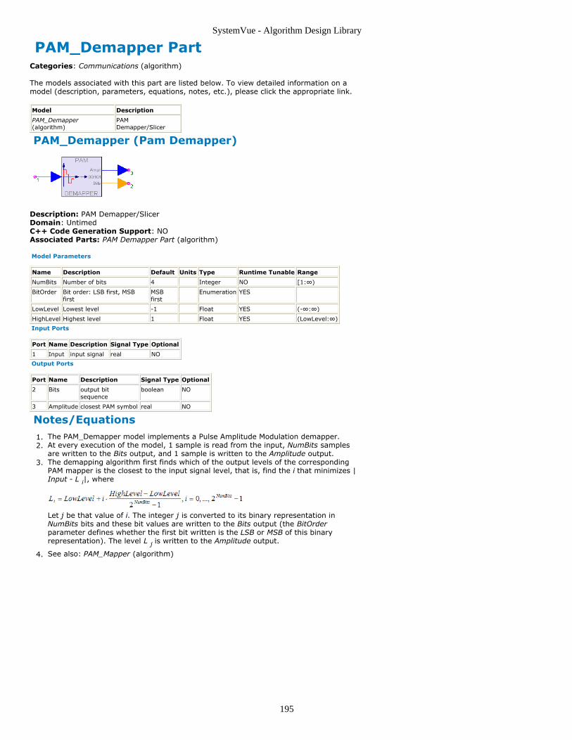
SystemVue - Algorithm Design Library
195
PAM_Demapper PartCategories: Communications (algorithm)
The models associated with this part are listed below. To view detailed information on amodel (description, parameters, equations, notes, etc.), please click the appropriate link.
Model Description
PAM_Demapper(algorithm)
PAMDemapper/Slicer
PAM_Demapper (Pam Demapper)
Description: PAM Demapper/SlicerDomain: UntimedC++ Code Generation Support: NOAssociated Parts: PAM Demapper Part (algorithm)
Model Parameters
Name Description Default Units Type Runtime Tunable Range
NumBits Number of bits 4 Integer NO [1:∞)
BitOrder Bit order: LSB first, MSBfirst
MSBfirst
Enumeration YES
LowLevel Lowest level -1 Float YES (-∞:∞)
HighLevel Highest level 1 Float YES (LowLevel:∞)
Input Ports
Port Name Description Signal Type Optional
1 Input input signal real NO
Output Ports
Port Name Description Signal Type Optional
2 Bits output bitsequence
boolean NO
3 Amplitude closest PAM symbol real NO
Notes/EquationsThe PAM_Demapper model implements a Pulse Amplitude Modulation demapper.1.At every execution of the model, 1 sample is read from the input, NumBits samples2.are written to the Bits output, and 1 sample is written to the Amplitude output.The demapping algorithm first finds which of the output levels of the corresponding3.PAM mapper is the closest to the input signal level, that is, find the i that minimizes |Input - L i|, where
Let j be that value of i. The integer j is converted to its binary representation inNumBits bits and these bit values are written to the Bits output (the BitOrderparameter defines whether the first bit written is the LSB or MSB of this binaryrepresentation). The level L j is written to the Amplitude output.
See also: PAM_Mapper (algorithm)4.

SystemVue - Algorithm Design Library
196
PAM_Mapper PartCategories: Communications (algorithm)
The models associated with this part are listed below. To view detailed information on amodel (description, parameters, equations, notes, etc.), please click the appropriate link.
Model Description
PAM_Mapper(algorithm)
PAM Mapper
PAM_Mapper (PAM Mapper)
Description: PAM MapperDomain: UntimedC++ Code Generation Support: NOAssociated Parts: PAM Mapper Part (algorithm)
Model Parameters
Name Description Default Units Type Runtime Tunable Range
NumBits Number of bits 4 Integer NO [1:∞)
BitOrder Bit order: LSB first, MSBfirst
MSBfirst
Enumeration YES
LowLevel Lowest level -1 Float YES (-∞:∞)
HighLevel Highest level 1 Float YES (LowLevel:∞)
Input Ports
Port Name Description Signal Type Optional
1 input input bits boolean NO
Output Ports
Port Name Description Signal Type Optional
2 output output PAM symbol real NO
Notes/EquationsThe PAM_Mapper model implements a Pulse Amplitude Modulation mapper.1.At every execution of the model, NumBits samples (bits) are read from the input and2.mapped into a level between LowLevel and HighLevel, which is then written to theoutput.The mapping algorithm first converts the NumBits bits read from the input (a 0 input3.value is considered to be a 0 bit; any other value is considered to be a 1 bit) into theequivalent integer representation (the BitOrder parameter defines whether the firstbit read is to be considered as LSB or MSB in this bit to integer conversion). Let thisinteger be i (the range of values i can have is 0 to 2 NumBits − 1). Then the outputlevel is given by
See also: PAM_Demapper (algorithm)4.

SystemVue - Algorithm Design Library
197
Scrambler PartCategories: Communications (algorithm)
The models associated with this part are listed below. To view detailed information on amodel (description, parameters, equations, notes, etc.), please click the appropriate link.
Model Description
Scrambler(algorithm)
Bit SequenceScrambler
Scrambler (Bit Sequence Scrambler)
Description: Bit Sequence ScramblerDomain: UntimedC++ Code Generation Support: NOAssociated Parts: Scrambler Part (algorithm)
Model Parameters
Name Description Default Units Type RuntimeTunable
Polynomial Generator polynomial for the shift register - decimal,octal, or hex integer
147457 Integer NO
ShiftReg Initial state of the shift register - decimal, octal, or hexinteger
1 Integer NO
Input Ports
Port Name Description Signal Type Optional
1 input input bit sequence (zero ornonzero)
boolean NO
Output Ports
Port Name Description Signal Type Optional
2 output output bit sequence (zero orone)
boolean NO
Notes/Equations
This component scrambles the input bit sequence using a feedback shift register, as1.shown in Feedback Shift Register. The taps of the feedback shift register are given bythe Polynomial parameter, which should be a positive integer. The nth bit of thisinteger indicates whether the nth tap of the delay line is fed back. The low-order bitis called the 0th bit, and must be set. The next low-order bit indicates whether theoutput of the first delay should be fed back, and so on. The default Polynomial is anoctal number defining the V.22bis scrambler.In scramblers based on feedback shift registers, all the bits to be fed back are2.exclusive-ORed together (their parity is calculated), and the result is exclusive-ORedwith the input bit. This result is produced at the output and shifted into the delayline. With proper choice of polynomial, the resulting output appears highly randomeven if the input is highly non-random (for example, all 0s or all 1s).
Feedback Shift Register
If the polynomial is a primitive polynomial, then the feedback shift register is a so-3.called maximal length feedback shift register. This means that with a constant input,the output will be sequence with period 2N -1 where N is the order of the polynomial(the length of the shift register). This is the longest possible sequence. Moreover,within this period the sequence will appear to be white, in that a calculatedautocorrelation will be very nearly an impulse. Therefore, the scrambler with aconstant input can be very effectively used to generate a pseudo-random bitsequence.The maximal-length feedback shift register with constant input will pass through 2N -1 states before returning to a state it has been in before. This is one short of the 2N

SystemVue - Algorithm Design Library
198
states that a register with N bits can take on. This one missing state, in fact, is alock-up state, in that if the input is an appropriate constant, the scrambler will ceaseto produce random-looking output, and will output a constant. For example, if theinput is all zeros, and the initial state of the scrambler is zero, then the outputs willbe all zero, hardly random. This is easily avoided by initializing the scrambler to somenon-0 state. That is why the default value for the ShiftReg parameter is set to 1.The Polynomial parameter must be carefully chosen. It must represent a primitive4.polynomial, which is one that cannot be factored into two (nontrivial) polynomialswith binary coefficients. For details, refer to [1].The table below lists primitive polynomials (expressed as octal numbers so that these5.are easily translated into taps on shift register); these will result in maximal-lengthpseudo-random sequences if the input is constant and lockup is avoided.Order Polynomial Order Polynomial Order Polynomial
11 04005 21 010000005
2 07 12 010123 22 020000003
3 013 13 020033 23 040000041
4 023 14 042103 24 0100000207
5 045 15 0100003 25 0200000011
6 0103 16 0210013 26 0400000107
7 0211 17 0400011 27 01000000047
8 0435 18 01000201 28 02000000011
9 01021 19 02000047 29 04000000005
10 02011 20 04000011 30 010040000007
The leading 0 in the polynomials indicates an octal number. Note also that reversingthe order of the bits in any of these numbers will also result in a primitivepolynomial. Therefore, the default value for the Polynomial parameter is 0440001 inoctal, or "100 100 000 000 000 001" in binary. Reversing these bits we get "100 000000 000 001 001" in binary, or 0400011 in octal. This latter number is listed in thetable as the primitive polynomial of order 17. The order is the index of the highest-order non-0 bit in the polynomial, where the low-order bit has index 0.Because the polynomial and the feedback shift register are both implemented usingtype int, the order of the polynomial is limited by the size of the int data type. Forsimplicity and portability, the polynomial is also not allowed to be interpreted as anegative integer, so the sign bit cannot be used. Therefore, if int is a 32-bit word,then the highest order polynomial allowed is 30 (recall that indexing for the orderstarts at 0, and we cannot use the sign bit). The primitive polynomials in the tableare up to order 30 because of 32-bit integer machines.Both the Polynomial and ShiftReg parameters can be set to a decimal, octal, or hexvalue. To enter an octal or hex value, prefix it with 0 or 0x, respectively. Forexample, in order to use the primitive polynomial of order 11, set Polynomial to04005, 0x805, or 2053.See also, DeScrambler (algorithm).6.
References
Lee and Messerschmitt, Digital Communication, Second Edition, Kluwer Academic1.Publishers, 1994, pp. 595-603.

SystemVue - Algorithm Design Library
199
ViterbiDecoder PartCategories: C++ Code Generation (algorithm), Communications (algorithm)
The models associated with this part are listed below. To view detailed information on amodel (description, parameters, equations, notes, etc.), please click the appropriate link.
Model Description
ViterbiDecoder(algorithm)
Viterbi Decoder for ConvolutionalCode
ViterbiDecoder (Viterbi Decoder for ConvolutionalCode)
Description: Viterbi Decoder for Convolutional CodeDomain: UntimedC++ Code Generation Support: YESAssociated Parts: ViterbiDecoder Part (algorithm)
Model Parameters
Name Description Default Units Type RuntimeTunable
CodingRate Coding rate: rate_1_2, rate_1_3,rate_1_4, rate_1_5, rate_1_6, rate_1_7,rate_1_8
rate_1_2 Enumeration NO
ConstraintLength Constraint length 7 Integer NO
Polynomial Generator polynomial [91, 121] Integerarray
NO
ZeroTail Zero tail used to convert convolutionalcode to block code: NO, YES
NO Enumeration NO
BitSequenceLength Length of bit squence not including tailbits
88 Integer NO
MaxSurvivorLength Maximum length of survivor in bits 35 Integer NO
Polarity Mapping mode from NRZ to logic signal:Negative to logic 1, Negative to logic 0
Negative tologic 1
Enumeration NO
InitialState Initial state of convolutional encoder:Zero state, Non-zero state
Zero state Enumeration NO
IgnoreNumber Number of data points to be ignored 0 Integer NO
Input Ports
Port Name Signal Type Optional
1 In real NO
Output Ports
Port Name Signal Type Optional
2 Out boolean NO
Notes/Equations
The ViterbiDecoder model is used for convolutionally decoding the input information1.sequence with a Viterbi algorithm.If ZeroTail = NO, this model reads (1/R) samples from input In and writes 1 sample2.to output Out. If ZeroTail = YES, this model reads (N + K − 1)/R samples from inputIn and writes (N + K − 1) samples to output Out. R = 1/2, 1/3, 1/4, 1/5, 1/6, 1/7, or1/8 when CodingRate = rate_1_2, rate_1_3, rate_1_4, rate_1_5, rate_1_6,rate_1_7, or rate_1_8 respectively.For example, the CDMA access channel CC(3, 1, 9) is defined with convolutional code3.rate R = 1/3 and K = 9. When ZeroTail = YES and N = 88, then this model reads 288samples from input In and writes 96 samples to output Out.Generally, there are two ways to implement convolutional code in communications4.system: code a semi-infinite bit sequence length where the initial encoder state couldbe zero- or non-zero with any final state; or, code block-by-block by appending zerotails after bit blocks so that the initial and the final encoder states are both zero. TheZeroTail parameter specifies this implementation; if ZeroTail = YES, then zero tailsmust be appended before input to this component.ViterbiDecoder supports the 1/ n coding rate only. Convolutional codes with k/ n ( k5.>1) are not supported by this component because: the coding and decoding will bemore complex (this is also the reason why convolutional codes with a k/n (k >1)coding rate are seldom used in real communication systems); and, evenconvolutional codes with a k/ n (k >1) coding rate are used that are typically

SystemVue - Algorithm Design Library
200
implemented by puncturing the convolutional code with a 1/ n coding rate.Polynomial is the convolutional code generator function. The generator matrix for a6.convolutional code is generally semi-infinite because the input sequence is semi-infinite. As an alternative to specifying the generator matrix, a functionally equivalentrepresentation is used in which a set of n vectors is specified, one vector for each ofthe n modulo-2 adder. 1 in the ith position of the vector indicates that thecorresponding stage in the shift register is connected to the modulo-2 adder; 0 in agiven position indicates that no connection exists between that stage and themodulo-2 adder.For example, consider the binary convolutional encoder with constraint length K = 7,k = 1, and n = 2, illustrated in Convolutional Code CC(2,1,7). The connection for y0is (1, 0, 1, 1, 0, 1, 1) from Outputs to Input, while the connection for y1 is (1, 1, 1,1, 1, 0, 1). Generators for this code are conveniently given in octal form as (0133,0175). So, when k=1, n generators (each of dimension K) are required to specify theencoder.
Convolutional Code CC(2,1,7)
ZeroTail is used to specify the encoder input sequence character. If ZeroTail = YES,7.the encoder input sequence is divided into blocks; block length is N . After eachblock, K−1 zeros are appended as tail bits. The total block length of the encoder is (N+ K − 1), referring to Tail bits removal for ZeroTail = YES. In the decoder, knowninformation can be used to obtain better performance.
Tail bits removal for ZeroTail = YES
BitSequenceLength (valid only when ZeroTail = YES) is used to specify the8.information bit length, which indicates the length of uncoded bits. This parameter canbe set to the same value in the encoder and the decoder.MaxSurvivorLength is the maximum length of the survivor that is stored in memory.9.The delay in decoding a long information sequence that has been convolutionallyencoded is usually too long for most practical applications; moreover, memoryrequired to store the entire length of surviving sequences is large and expensive. Asolution for this is to modify the Viterbi algorithm in such a way that results in a fixeddecoding delay without significantly affecting the optimal performance of thealgorithm.The modification is to retain at any given time t only the most recent δ decodedinformations bits in each surviving sequence. As each new information bit is received,a final decision is made on the bit received δ branches back in the trellis, bycomparing the metrics in the surviving sequences and determining in favor of the bitin the sequence having the largest metric. If the δ chosen is sufficiently large, allsurviving sequences will contain the identical decoded bit δ branches back in time.That is, with high probability, all surviving sequences at time t stem from the sameone as t−. Experimental simulation has determined that a delay δ ≥ 5 K results in anegligible degradation in the performance relative to the optimum Viterbi algorithm.Polarity is used to specify the mapping mode from bit (0, 1) to the NRZ signal level.10.Generally, bit 0 is mapped to level 1 and bit 1 is mapped level −1. An alternative isto map bit 0 to level −1 and bit 1 to level 1.InitialState is used to specify the coded sequence character. If the initial state of11.encoder is zero-state, the known information can be used to obtain betterperformance. If the initial state is not known to be zero, InitialState must be set to anon-zero state.IgnoreNumber is used to specify how much data will be ignored by this component.12.Delays in communications systems can be caused by devices or transmission. And,the delay may be inserted between the encoder and decoder in the form ofmeaningless data, so the information must be set in IgnoreNumber.
If ZeroTail = YES, the value of IgnoreNumber is n × (N + K − 1)/ R (n is aninteger and n ≥ 0), and no extra delay will be introduced because it is assumed

SystemVue - Algorithm Design Library
201
the sequence is frame synchronized before input to ViterbiDecoder.If ZeroTail = NO, the delay is an integer number n ; this means the symbolsynchronization is achieved before ViterbiDecoder. If n / R is also an integer,then the delay of output bit sequence will be n / R bits. Otherwise, the delay willbe the minimum integer larger than n / R.Input sequence requirements are:If ZeroTail = YESThe input sequence must be frame synchronized; that is, IgnoreNumber mustbe n × N / R (n is an integer and n ≥ 0) and the first valid data must be thefirst symbol of the first codeword in that frame.The input sequence must be encoded from blocks, each having K−1 zero tails sothat the initial state and final state are all zero-state.If ZeroTail = NOThe input sequence must be bit synchronized; that is, the first valid data mustbe the first symbol of a codeword.If InitialState is set to Zero state, the first valid symbol must be encoded withzero initial state.
The Viterbi algorithm is an optimal method of decoding convolutional codes. Optimal13.decoding decisions cannot be made on a symbol-by-symbol basis; instead, the entirereceived sequence must be compared with all possible transmitted sequences. Thenumber of possible transmitted sequences increases exponentially with time, so anefficient method of comparing sequences is necessary.The Viterbi algorithm is computationally efficient, but its complexity increasesexponentially with the constraint length of the code. The Viterbi decoder measureshow similar the received sequence is to a transmitted sequence by calculating anumber called path metric (path metric of a sequence is calculated by addingnumbers known as symbol metric, which is a measure of how close a receivedsymbol is to each of the possible transmitted symbols). The transmitted sequencecorresponding to the smallest path metric is declared to be the most likely sequence.The Viterbi algorithm for a CC(n, k, K) code is described in the following paragraphs.Branch Metric CalculationThe branch metric m (a)
j , at the J th instant of the α path through the trellis is
defined as the logarithm of the joint probability of the received n-bit symbol r j 1, r j
2 ... , r jn conditioned on the estimated transmitted n-bit symbol c j 1 (a) , c j 2 (a) ...
, c jn(a) for the α path. That is,
If Rake receiver is regarded as a part of the channel, for the Viterbi decoder thechannel can be considered to be an AWGN channel. Therefore,
Path Metric CalculationThe path metric M (a) for the α path at the J th instant is the sum of the branchmetrics belonging to the α path from the first instant to the J th instant. Therefore,
Information Sequence UpdateThere are 2 k merging paths at each node in the trellis and the decoder selects frompaths α1, α2, ... , α2k the one having the largest metric, namely:
This path is known as the survivor.Decoder OutputWhen the two survivors have been determined at the J th instant, the decoderoutputs from memory the ( J-L )th information symbol survivor with the largestmetric.ViterbiDecoder Component Validation14.BER Measurements lists BER measurements for a rate 1/2 code (g 0 = 171, g 1 =
133) and a memoryless additive white Gaussian channel. Simulations were madewith hard decision decoding (binary quantization) and soft decision decoding (noquantization). Simulation results are listed along with results published inQUALCOMM Technical Data Sheet Q0256; note that the published data andsimulation results agree.As can be seen from this table, there is a substantial BER performance improvementwhen this model is used with soft decision decoding. The difference between the twodecoding processes is whether the input to this model is a binary signal (NRZ with -1and 1 levels) or is an analog signal (the raw NRZ signal with noise and intersymbol

SystemVue - Algorithm Design Library
202
interference included). Where possible, use this model with an input analog signalwith no binary decision made before this model. By providing the raw analog signalto the input of this model the model can then perform the soft decision decoding thatresults in superior BER performance.
Eb/No(dB) Hard Decision Soft Decision
Simulated BER QUALCOMM BER Simulated BER QUALCOMM BER (3 bits)
3.0 3.62e-04 8.00e-04
3.5 7.56e-05 2.00e-04
4.0 5.01e-03 6.50e-03 1.11e-05 3.50e-05
4.5 1.79e-03 1.80e-03 2.12e-06 7.00e-06
5.0 5.71e-04 5.50e-04
5.5 1.25e-04 9.00e-05
6.0 2.81e-05 4.00e-05
See Also:
ConvolutionalCoder (algorithm)
References
S. Lin and D. J. Costello, Jr., Error Control Coding Fundamentals and Applications,1.Prentice Hall, Englewood Cliffs NJ, 1983.J. G. Proakis, Digital Communications (Third edition), Publishing House of Electronics2.Industry, Beijing, 1998.

SystemVue - Algorithm Design Library
203
ADSCosimBlock PartCategories: Cosimulation (algorithm)
The models associated with this part are listed below. To view detailed information on amodel (description, parameters, equations, notes, etc.), please click the appropriate link.
Model Description
ADSCosimBlock (algorithm) ADS cosimulation
ADSCosimBlockCx (algorithm) ADS cosimulation for complex signal
ADSCosimBlockEnv(algorithm)
ADS cosimulation for envelopesignal
ADSCosimBlock
Description: ADS cosimulationDomain: UntimedC++ Code Generation Support: NOAssociated Parts: ADSCosimBlock Part (algorithm)
Model Parameters
Name Description Default Units Type RuntimeTunable
InputBlockSize Array of numbers of input samples per port.The receiving end should set the same value.
[1] None NO
OutputBlockSize Array of numbers of output samples per port.The sending end should set the same value.
[1] None NO
InputID Identification for shared memory. Thereceiving end should set the same ID.
SystemVueToADS Text NO
OutputID Identification for shared memory. The sendingend should set the same ID.
ADSToSystemVue Text NO
Input Ports
Port Name Signal Type Optional
1 input multiple real NO
Output Ports
Port Name Signal Type Optional
2 output multiple real NO
Notes/Equations
ADSCosimBlock performs SystemVue-ADS cosimulation by transferring double-type1.data samples between this model and the corresponding cosimulation blocks in ADSthrough shared memory.This model consumes InputBlockSize numbers of samples from input ports and2.produces OutputBlockSize numbers of samples to output ports in every execution.InputBlockSize is an array parameter specifying numbers of samples to be3.consumed for each of the input ports.OutputBlockSize is an array parameter specifying numbers of samples to be4.produced to each of the output ports.InputID specifies the shared memory identifier for transferring samples from the5.input port to the corresponding block SVCosimSourceDbl in ADS.outputID specifies the shared memory identifier for transferring samples from the6.corresponding block SVCosimSinkDbl in ADS to the output port.The input data samples are transferred to the corresponding ADS block7.SVCosimSourceDbl using shared memory. The InputBlockSize parameter inADSCosimBlock and the BlockSize parameter in ADS SVCosimSourceDbl should beset to the same value. The InputID parameter in ADSCosimBlock and theSVSenderID parameter in ADS SVCosimSourceDbl should be set to the sameidentifier string.The output data samples are transferred from the corresponding ADS block8.SVCosimSinkDbl using shared memory. The OutputBlockSize parameter inADSCosimBlock and the BlockSize parameter in ADS SVCosimSinkDbl should be setto the same value. The OutputID parameter in ADSCosimBlock and theSVReceiverID parameter in ADS SVCosimSinkDbl should be set to the sameidentifier string.The cosimulation library for ADS2009U1 is provided in9.\Examples\SV_ADS_Link\ADS2009U1\adsptolemy.zip under SystemVue installationdirectory. To load the cosimulation library in ADS, set ADSPTOLEMY_MODEL_PATHenvironment variable to "adsptolemy" directory (note that the path cannot contain

SystemVue - Algorithm Design Library
204
any space). After starting ADS, the cosimulation blocks can be found in "SystemVueCosimulation" category. For more details about custom models in ADS, please refertohttp://edocs.soco.agilent.com/display/ads2009U1/Building+Signal+Processing+Models.
The cosimulation library for ADS2011.01 32bit is provided in10.\Examples\SV_ADS_Link\ADS2011.01\adsptolemy.zip under SystemVue installationdirectory.SystemVue-ADS cosimulation example workspaces can be found in11.\Examples\SV_ADS_Link under SystemVue installation directory.When using this model for SystemVue-ADS cosimulation, both SystemVue and ADS12.workspaces should be opened and simulated on the same machine.Use ADSCosimBlockCx (algorithm) for complex data type cosimulation. Use13.ADSCosimBlockEnv (algorithm) for timed envelope data type cosimulation.Please refer to application note14.http://edocs.soco.agilent.com/display/eesofkc/SystemVue+ADS+link+bidirectional+cosim+3-in-1+example+LTE+HD+WPAN+ZigBee for details in SystemVue-ADS cosimulationexamples. The application note also provides template projects for creating customcosimulation models.
ADSCosimBlockCx
Description: ADS cosimulation for complex signalDomain: UntimedC++ Code Generation Support: NOAssociated Parts: ADSCosimBlock Part (algorithm)
Model Parameters
Name Description Default Units Type RuntimeTunable
InputBlockSize Array of numbers of input samples per port.The receiving end should set the same value.
[1] None NO
OutputBlockSize Array of numbers of output samples per port.The sending end should set the same value.
[1] None NO
InputID Identification for shared memory. Thereceiving end should set the same ID.
SystemVueToADS Text NO
OutputID Identification for shared memory. The sendingend should set the same ID.
ADSToSystemVue Text NO
Input Ports
Port Name Signal Type Optional
1 input multiple complex NO
Output Ports
Port Name Signal Type Optional
2 output multiple complex NO
Notes/Equations
ADSCosimBlockCx performs SystemVue-ADS cosimulation by transferring complex-1.type data samples between this model and the corresponding cosimulation blocks inADS through shared memory.This model consumes InputBlockSize numbers of samples from input ports and2.produces OutputBlockSize numbers of samples to output ports in every execution.The corresponding cosimulation blocks in ADS are SVCosimSourceCx and3.SVCosimSinkCx, which are provided in\Examples\SV_ADS_Link\ADS2009U1\adsptolemy under SystemVue installationdirectory.Please refer to ADSCosimBlock (algorithm) for detailed description and parameter4.specification.
ADSCosimBlockEnv
Description: ADS cosimulation for envelope signalDomain: TimedC++ Code Generation Support: NOAssociated Parts: ADSCosimBlock Part (algorithm)

SystemVue - Algorithm Design Library
205
Model Parameters
Name Description Default Units Type RuntimeTunable
OutputFc Array of characterization frequency of outputenvelope signal. The values should obtainedfrom the sending co-simulation process.
0 None NO
InputBlockSize Array of numbers of input samples per port. Thereceiving end should set the same value.
[1] None NO
OutputBlockSize Array of numbers of output samples per port.The sending end should set the same value.
[1] None NO
InputID Identification for shared memory. The receivingend should set the same ID.
SystemVueToADS Text NO
OutputID Identification for shared memory. The sendingend should set the same ID.
ADSToSystemVue Text NO
Input Ports
Port Name Signal Type Optional
1 input multipleenvelope
NO
Output Ports
Port Name Signal Type Optional
2 output multipleenvelope
NO
Notes/Equations
ADSCosimBlockCx performs SystemVue-ADS cosimulation by transferring envelope-1.type data samples between this model and the corresponding cosimulation blocks inADS through shared memory.This model consumes InputBlockSize numbers of samples from input ports and2.produces OutputBlockSize numbers of samples to output ports in every execution.The corresponding cosimulation blocks in ADS are SVCosimSourceTimed and3.SVCosimSinkTimed, which are provided in\Examples\SV_ADS_Link\ADS2009U1\adsptolemy under SystemVue installationdirectory.OutputFc is an array parameter specifying characterization frequencies for each of4.the output ports (output envelope signal). OutputFc should be set according to thecorresponding design in ADS.Please refer to ADSCosimBlock (algorithm) for detailed description and parameter5.specification.

SystemVue - Algorithm Design Library
206
ADSCosimSink PartCategories: Cosimulation (algorithm)
The models associated with this part are listed below. To view detailed information on amodel (description, parameters, equations, notes, etc.), please click the appropriate link.
Model Description
ADSCosimSink (algorithm) ADS cosimulation sink
ADSCosimSinkCx (algorithm) ADS cosimulation sink for complex signal
ADSCosimSinkEnv(algorithm)
ADS cosimulation sink for envelope signal
ADSCosimSink
Description: ADS cosimulation sinkDomain: UntimedC++ Code Generation Support: NOAssociated Parts: ADSCosimSink Part (algorithm)
Model Parameters
Name Description Default Units Type RuntimeTunable
InputBlockSize Array of numbers of input samples per port. Thereceiving end should set the same value.
[1] None NO
InputID Identification for shared memory. The receivingend should set the same ID.
SystemVueToADS Text NO
Input Ports
Port Name Signal Type Optional
1 input multiple real NO
Notes/Equations
ADSCosimSink performs SystemVue-ADS cosimulation by transferring double-type1.data samples from this model to the corresponding cosimulation block in ADSthrough shared memory.This model consumes InputBlockSize numbers of samples from input ports in2.every execution.InputBlockSize is an array parameter specifying numbers of samples to be3.consumed for each of the input ports.InputID specifies the shared memory identifier for transferring samples from the4.input port to the corresponding block SVCosimSourceDbl in ADS.The input data samples are transferred to the corresponding ADS block5.SVCosimSourceDbl using shared memory. The InputBlockSize parameter inADSCosimBlock and the BlockSize parameter in ADS SVCosimSourceDbl should beset to the same value. The InputID parameter in ADSCosimBlock and theSVSenderID parameter in ADS SVCosimSourceDbl should be set to the sameidentifier string.The cosimulation library for ADS2009U1 is provided in6.\Examples\SV_ADS_Link\ADS2009U1\adsptolemy.zip under SystemVue installationdirectory. To load the cosimulation library in ADS, set ADSPTOLEMY_MODEL_PATHenvironment variable to "adsptolemy" directory (note that the path cannot containany space). After starting ADS, the cosimulation blocks can be found in "SystemVueCosimulation" category. For more details about custom models in ADS, please refertohttp://edocs.soco.agilent.com/display/ads2009U1/Building+Signal+Processing+Models.
The cosimulation library for ADS2011.01 32bit is provided in7.\Examples\SV_ADS_Link\ADS2011.01\adsptolemy.zip under SystemVue installationdirectory.SystemVue-ADS cosimulation example workspaces can be found in8.\Examples\SV_ADS_Link under SystemVue installation directory.When using this model for SystemVue-ADS cosimulation, both SystemVue and ADS9.workspaces should be opened and simulated on the same machine.Use ADSCosimSinkCx (algorithm) for complex data type cosimulation. Use10.ADSCosimSinkEnv (algorithm) for timed envelope data type cosimulation.Please refer to application note11.http://edocs.soco.agilent.com/display/eesofkc/SystemVue+ADS+link+bidirectional+cosim+3-in-1+example+LTE+HD+WPAN+ZigBee for details in SystemVue-ADS cosimulationexamples. The application note also provides template projects for creating custom

SystemVue - Algorithm Design Library
207
cosimulation models.
ADSCosimSinkCx
Description: ADS cosimulation sink for complex signalDomain: UntimedC++ Code Generation Support: NOAssociated Parts: ADSCosimSink Part (algorithm)
Model Parameters
Name Description Default Units Type RuntimeTunable
InputBlockSize Array of numbers of input samples per port. Thereceiving end should set the same value.
[1] None NO
InputID Identification for shared memory. The receivingend should set the same ID.
SystemVueToADS Text NO
Input Ports
Port Name Signal Type Optional
1 input multiple complex NO
Notes/Equations
ADSCosimSinkCx performs SystemVue-ADS cosimulation by transferring complex-1.type data samples from this model to the corresponding cosimulation block in ADSthrough shared memory.This model consumes InputBlockSize numbers of samples from input ports in2.every execution.The corresponding cosimulation block in ADS is SVCosimSourceCx, which is provided3.in \Examples\SV_ADS_Link\ADS2009U1\adsptolemy under SystemVue installationdirectory.Please refer to ADSCosimSink (algorithm) for detailed description and parameter4.specification.
ADSCosimSinkEnv
Description: ADS cosimulation sink for envelope signalDomain: TimedC++ Code Generation Support: NOAssociated Parts: ADSCosimSink Part (algorithm)
Model Parameters
Name Description Default Units Type RuntimeTunable
InputBlockSize Array of numbers of input samples per port. Thereceiving end should set the same value.
[1] None NO
InputID Identification for shared memory. The receivingend should set the same ID.
SystemVueToADS Text NO
Input Ports
Port Name Signal Type Optional
1 input multipleenvelope
NO
Notes/Equations
ADSCosimSinkEnv performs SystemVue-ADS cosimulation by transferring envelope-1.type data samples from this model to the corresponding cosimulation block in ADSthrough shared memory.This model consumes InputBlockSize numbers of samples from input ports in2.every execution.The corresponding cosimulation block in ADS is SVCosimSourceTimed, which is3.provided in \Examples\SV_ADS_Link\ADS2009U1\adsptolemy under SystemVueinstallation directory.Please refer to ADSCosimSink (algorithm) for detailed description and parameter4.specification.

SystemVue - Algorithm Design Library
208
FastCircuitEnvelope PartCategories: Cosimulation (algorithm)
The models associated with this part are listed below. To view detailed information on amodel (description, parameters, equations, notes, etc.), please click the appropriate link.
Model Description
FastCircuitEnvelope(algorithm)
GoldenGate Fast Circuit Envelope
Fast Circuit Envelope
Description: GoldenGate Fast Circuit EnvelopeDomain: TimedC++ Code Generation Support: NOAssociated Parts: FastCircuitEnvelope Part (algorithm)
Model Parameters
Name Description Default Units Type RuntimeTunable
File Fast Circuit Envelope file Filename NO
OutOfRangeOption Option when input signal is out of range:Clip, Extrapolate
Clip Enumeration NO
Notes/Equations
The FastCircuitEnvelope model can load and simulate the fast circuit envelope file(model) extracted from GoldenGate.Please refer to GoldenGate document for how to extract fast circuit envelope modelsfrom your circuits.The sections below describe how to load, set, and use the extracted fast circuitenvelope model from GoldenGate.Users should use the FastCircuitEnvelope UI (shown below) to configure the settings,except for OutOfRangeOption.Parameter OutOfRangeOption can be set inside Advanced Options. When inputsignals are out of range, Clip option clips the input signals and Extrapolate optionextrapolates the input signals.Fast circuit envelope examples can be found in \Examples\RF ArchitectureDesign\GoldenGate under SystemVue installation directory.GoldenGate supports fast circuit envelope extraction for level 1 and level 3 models.These types of models are very accurate for many applications, but please be awareof the following limitations:
Level 1 models capture only the nonlinear characteristics of the circuit in the center of the operatingband, including harmonic content. Additionally, nonlinear behavior is only captured over a certainrange of input amplitudes. SystemVue will warn you if you apply input signals above or below thecharacterization range. Noise and memory effects are NOT modeled in Level 1 models. The inputand output impedance is fixed based on how it was loaded during extraction.
Level 3 models capture only the nonlinear characteristics of a circuit over a specified band offrequencies. Additionally, nonlinear behavior is only captured over a certain range of inputamplitudes. SystemVue will warn you if you apply input signals above or below the characterizationrange in terms of either amplitude or frequency. Memory effects are captured in Level 3 models.Noise effects are not currently modeled in Level 3 models. The input and output impedance is fixedbased on how it was loaded during extraction.
ComparisonThe table below compares how different effects are supported between fast circuitenvelope level 1, fast circuit envelope level 3, direct GoldenGate circuit cosimulation(algorithm) (envelope transient), and X-parameters (rfdesign).

SystemVue - Algorithm Design Library
209
Effect Fast CircuitEnvelopeLevel 1
Fast CircuitEnvelopeLevel 3
GoldenGateCircuit(algorithm)Cosimulation(algorithm)
X-parameters(rfdesign)
Power dependence Within extractedrange
Within extractedrange
Unlimited Within extractedrange
Memory (Inband and Baseband) No Yes Yes No
Memory (Frequencydependence with respect to RFcenter frequency)
(see note 1) (see note 1) Yes (see note 1)
Load dependence (see note 1) (see note 1) (see note 1) Good
DC dependence (see note 1) Within extractedrange
(see note 1) Within extractedrange
Noise No No Within extractedrange
No
Frequency translation Yes Yes Yes Yes
Licenses used for extraction GoldenGate:EnvelopeTransient
GoldenGate:EnvelopeTransient
None ADS: W2305 X-parameterGenerator
Licenses used forrun-time simulation
SystemVue:W1719 RFSystem
SystemVue:W1719 RFSystem
SystemVue: BaseenvironmentGoldenGate:Envelope Transient
SystemVue:W1719 RF System
Note 1 - The value for this parameter is constant, based on how it was set during themodel extraction process. However, selecting between multiple individual models canaccomplish useful parameterization of this quantity.
Part Properties Fast Envelope Settings Page
Browse – Click this button to load a GoldenGate .fce file. Once the .fce file is loaded,the input and output ports will be configured automatically.
Name – The port name in the .fce file.Use – Check to include the associated output port on the schematic symbol, so thatthe output signal from the port can be obtained and used during simulation.Direction – Port direction, Input or Output.Input Range – Shows the acceptable voltage range for the input signal. If the inputsignal is out of range, it is either clipped or extrapolated based on theOutOfRangeOption (Clip by default).Characterization Frequency – Select a frequency (or "All") from the dropdown. If aparticular frequency is selected, the port outputs the signal associated with thatcharacterization frequency (harmonic). On the other hand, if "All" is selected, signalsassociated with all characterization frequencies (harmonics) are outputted through amulti-port (bus), in the same order as listed in the dropdown.Manage Outputs – Click to display the Manage Outputs dialog box, as describedbelow.
Manage Outputs
If you click the Manage Outputs button on the Fast Circuit Envelope Properties dialog box,the following dialog box is displayed. It's basically just an enlarged version of the mainsettings page, with more room for outputs and additional controls to simplify using morecomplex GoldenGate models.

SystemVue - Algorithm Design Library
210
Only show ports currently in use – When checked, only those ports which have acheckmark in the Use column will be displayed; the others are hidden. Also affectsthe page in the main Properties dialog box.Check All – Click to place a checkmark in the Use column of all output ports.Uncheck All – Click to remove all the Use checkmarks.
Tip: To check (or uncheck) a group of ports, click the Use checkbox of the first port you'd like to change,then hold down the Shift key while clicking the last port you'd like to change.
Details Page
The Details page displays the fast circuit envelope information of the .fce file. A LNA fastcircuit envelope example is shown below.
Design: 'SIM_LNA_ENV_ET' -- A test with a lot of output ports.
Created by: GoldenGate (release ver. 4.5.425-DEV build 2231 -- Jan 10 2011)
Created on: Tue Jan 11 02:42:49 2011
Model Extraction Info:
• Model Bandwidth: 7.373e+6 Hz
• Integration Order: 1
• Number of Source Sweep Points: 20
• Frequency Sweep Resolution: 1 Hz
Fundamental Frequencies (Hz):
• 5.25e+9
Output Carrier Tones (Hz):
• 0: Index=(0, 0, 0)
• 5.25e+9: Index=(1, 0, 0)
Input Ports:
• RF_IN Range=(17.39e-6, 1.739e-3) Freq=5.25e+9 Hz Index=(1, 0, 0)
Output Ports:
• RF
• LNA_I
• LNA_Q

SystemVue - Algorithm Design Library
211
All output ports are extracted with the same set of characterization frequencies listed in "Output CarrierTones".

SystemVue - Algorithm Design Library
212
GoldenGateCosim PartCategories: Cosimulation (algorithm)
The models associated with this part are listed below. To view detailed information on amodel (description, parameters, equations, notes, etc.), please click the appropriate link.
Model Description
GoldenGateCosim(algorithm)
GoldenGatecosimulation
GoldenGateCosim
Description: GoldenGate cosimulationDomain: TimedC++ Code Generation Support: NOAssociated Parts: GoldenGateCosim Part (algorithm)
Model Parameters
Name Description Default Units Type Runtime Tunable
Path Path from home directory to GoldenGate script Text NO
BlockSize Block size for cosimulation communication 1 Integer NO
Notes/Equations
The GoldenGateCosim model cosimulates with GoldenGate Envelope Transientsimulator for the exported GoldenGate netlist.In every execution, this model consumes BlockSize number of samples from eachinput port, sends the samples over network to GoldenGate, waits for GoldenGate tosimulate BlockSize time points (continuously at the sampling rate associated with thismodel), then receives samples from GoldenGate, and produces BlockSize number ofsamples at each output port.Please refer to GoldenGate document about how to export your circuits fromGoldenGate for SystemVue cosimulation.The sections below describe how to import the netlist and set up the model forcosimulation.Users should use the GoldenGateCosim UI (shown below) to configure the settings,except for BlockSize.Parameter BlockSize can be set inside Advanced Options. It represents the numberof samples to be transferred across network in chunk. For small-scale circuit,increasing BlockSize can reduce communication and synchronization overhead. Forlarge-scale circuit, the overhead is negligible because Envelope Transient simulationis slow in nature comparing to data flow simulation.Please refer to Fast Circuit Envelope (algorithm) document for using fast circuitenvelope models extracted from GoldenGate.GoldenGate cosimulation examples can be found in \Examples\RF ArchitectureDesign\GoldenGate under SystemVue installation directory.
The comparison chart (algorithm) in the FastCircuitEnvelope (algorithm) document page comparesadvantages and limitations between GoldenGate cosimulation, Fast Circuit Envelope (algorithm) level 1and level 3, and X-Parameters (rfdesign).
Please set up Distributed Simulations (sim) first before using the GoldenGateCosim model.
Part Properties GoldenGate Cosimulation Settings Page
Place down a new GoldenGateCosim part on a schematic, double click the part, you willsee the following GoldenGate Cosimulation Settings page.
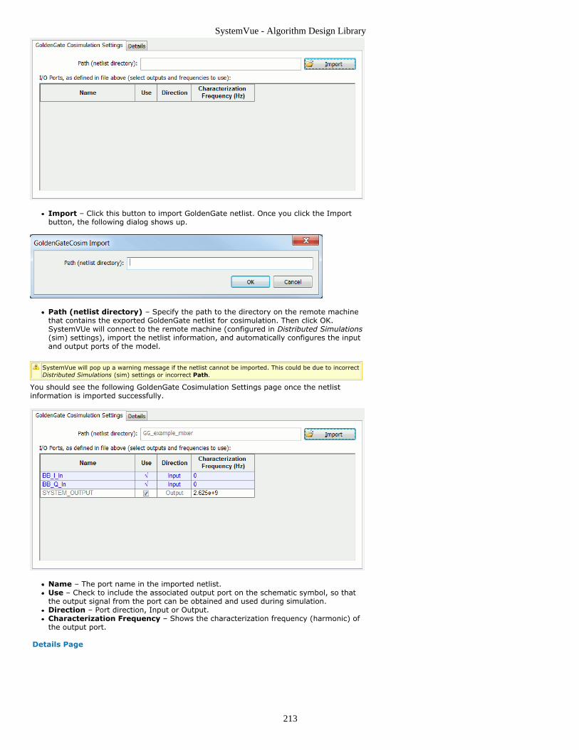
SystemVue - Algorithm Design Library
213
Import – Click this button to import GoldenGate netlist. Once you click the Importbutton, the following dialog shows up.
Path (netlist directory) – Specify the path to the directory on the remote machinethat contains the exported GoldenGate netlist for cosimulation. Then click OK.SystemVUe will connect to the remote machine (configured in Distributed Simulations(sim) settings), import the netlist information, and automatically configures the inputand output ports of the model.
SystemVue will pop up a warning message if the netlist cannot be imported. This could be due to incorrectDistributed Simulations (sim) settings or incorrect Path.
You should see the following GoldenGate Cosimulation Settings page once the netlistinformation is imported successfully.
Name – The port name in the imported netlist.Use – Check to include the associated output port on the schematic symbol, so thatthe output signal from the port can be obtained and used during simulation.Direction – Port direction, Input or Output.Characterization Frequency – Shows the characterization frequency (harmonic) ofthe output port.
Details Page

SystemVue - Algorithm Design Library
214
The Details page displays the imported netlist information. For example, the netlistinformation of a mixer example is shown below.
Design: 'SIM_IQ_MOD_ENV'
Created by: GoldenGate (release ver. 4.5.448-DEV build 2254 -- Feb 1 2011)
Created on: Feb 17 19:00:33 2011
Fundamental Frequencies (Hz):
• 2.625e+9
Output Carrier Tones (Hz):
• 0
• 2.625e+9
• 5.25e+9
Input Ports:
• BB_I_In Freq=0 Hz
• BB_Q_In Freq=0 Hz
Output Ports:
• SYSTEM_OUTPUT

SystemVue - Algorithm Design Library
215
DynamicPack_M PartCategories: Dynamic (algorithm), Math Matrix (algorithm), Type Converters (algorithm)
The models associated with this part are listed below. To view detailed information on amodel (description, parameters, equations, notes, etc.), please click the appropriate link.
Model Description
DynamicPack_M(algorithm)
Pack variable numbers of samples intomatrices
DynamicPack_M
Description: Pack variable numbers of samples into matricesDomain: UntimedC++ Code Generation Support: NOAssociated Parts: DynamicPack M Part (algorithm)
Model Parameters
Name Description Default Units Type RuntimeTunable
Format Format of data to be packed into matrix:ColumnMajor, RowMajor
ColumnMajor Enumeration NO
Input Ports
Port Name Description Signal Type Optional
1 input Input samples anytype NO
2 numRows Control signal for number of rows int YES
3 numColumns Control signal for number of columns int YES
Output Ports
Port Name Description Signal Type Optional
4 output Outputmatrix
anytype matrix NO
Notes/Equations
DynamicPack_M packs variable numbers of input samples into output matrices based1.on numRows and numColumns control signals.A complete execution consists of two modes: control mode and operation mode.2.In control mode, DynamicPack_M reads one sample from numRows and one sample3.from numColumns, and the integer values specify number-of-rows and number-of-columns respectively for the matrix to be packed in the operation mode.In operation mode, DynamicPack_M reads number-of-rows * number-of-columns4.number of samples from input, then packs them into number-of-rows by number-of-columns output matrix in either column major or row major according to the Formatparameter.If numRows is not connected, number-of-rows is default to be 1, which means a row5.vector. If numColumns is not connected, number-of-columns is default to be 1, whichmeans a column vector. At least one of the control inputs (numRows, numColumns)must be connected.The integer value for number-of-rows or number-of-columns can be 0 or negative,6.which results in an empty matrix.
See:DynamicUnpack_M (algorithm)Pack_M (algorithm)Unpack_M (algorithm)

SystemVue - Algorithm Design Library
216
DynamicUnpack_M PartCategories: Dynamic (algorithm), Math Matrix (algorithm), Type Converters (algorithm)
The models associated with this part are listed below. To view detailed information on amodel (description, parameters, equations, notes, etc.), please click the appropriate link.
Model Description
DynamicUnpack_M(algorithm)
Unpack variable-size matrices intosamples
DynamicUnpack_M
Description: Unpack variable-size matrices into samplesDomain: UntimedC++ Code Generation Support: NOAssociated Parts: DynamicUnpack M Part (algorithm)
Model Parameters
Name Description Default Units Type RuntimeTunable
Format Format of data to be packed into matrix:ColumnMajor, RowMajor
ColumnMajor Enumeration NO
Input Ports
Port Name Description Signal Type Optional
1 input Input matrix anytype matrix NO
Output Ports
Port Name Description Signal Type Optional
2 output Output samples anytype NO
3 numRows Number of rows int NO
4 numColumns Number ofcolumns
int NO
Notes/Equations
DynamicUnpack_M unpacks variable-size input matrices into output samples.1.A complete execution consists of two modes: control mode and operation mode.2.In control mode, DynamicUnpack_M reads one matrix from input. Suppose the size of3.the matrix is number-of-rows by number-of-columns.In operation mode, DynamicUnpack_M unpacks the matrix into number-of-rows *4.number-of-columns number of output samples in either column major or row majoraccording to the Format parameter. It also writes number-of-rows integer value tonumRows and writes number-of-columns integer value to numColumns.If an input matrix is empty, DynamicUnpack_M will not generate any sample at5.output, but still write 0 to numRows and 0 to numColumns.
See:DynamicPack_M (algorithm)Pack_M (algorithm)Unpack_M (algorithm)

SystemVue - Algorithm Design Library
217
FiltersThe Filters library contains various digital (discrete-time) filters for signal processing.These filters are implemented as either digital FIR (finite impulse response) or digital IIR(infinite impulse response) filters.
For details, please refer Common Filter Parameters (algorithm)
ContentsBiquad Part (algorithm)BiquadCascade Part (algorithm)BlockAllPole Part (algorithm)BlockFIR Part (algorithm)Filter Part (algorithm)FIR Part (algorithm)Hilbert Part (algorithm)IIR Part (algorithm)OSF Part (algorithm)PID Part (algorithm)SData Part (algorithm)SDomainIIR Part (algorithm)

SystemVue - Algorithm Design Library
218
BiquadCascade PartCategories: C++ Code Generation (algorithm), Filters (algorithm)
The models associated with this part are listed below. To view detailed information on amodel (description, parameters, equations, notes, etc.), please click the appropriate link.
Model Description
BiquadCascade(algorithm)
IIR Filter with Cascaded Biquad Sections
BiquadCascade (IIR Filter with Cascaded BiquadSections)
Description: IIR Filter with Cascaded Biquad SectionsDomain: UntimedC++ Code Generation Support: YESAssociated Parts: BiquadCascade Part (algorithm)
Model Parameters
Name Description Default Units Type RuntimeTunable
Taps Sets of six biquadcoefficients.
[0.067455, 0.135, 0.067455, 1, -1.143, 0.4128]
Floating pointarray
NO
Input Ports
Port Name Description Signal Type Optional
1 input real NO
Output Ports
Port Name Description SignalType
Optional
2 output The outputs from each of the biquads in the cascade, starting with theoutput from last.
multiplereal
NO
Notes/Equations
BiquadCascade is a cascade of 2-pole, 2-zero digital IIR filter (a biquad). This IIR1.filter has a Z-domain transfer function of
For every input, one filtered value is output.2.Each biquad section is defined by six coefficients in order: N 0,i N 1,i N 2,i D 0,i D 1,i D3.
2,i .
The multi-output pin contains each of the outputs of the cascade, starting with the4.output from the last.The default is a single biquad Butterworth filter with a frequency cutoff at 0.1 of the5.input rate.
See:Biquad (algorithm)IIR (algorithm)IIR_Cx (algorithm)
References
A. V. Oppenheim and R. W. Schafer, Discrete-Time Signal Processing, Prentice-Hall:1.Englewood Cliffs, NJ, 1989.

SystemVue - Algorithm Design Library
219
Biquad PartCategories: C++ Code Generation (algorithm), Filters (algorithm)
The models associated with this part are listed below. To view detailed information on amodel (description, parameters, equations, notes, etc.), please click the appropriate link.
Model Description
Biquad(algorithm)
Biquad IIRFilter
Biquad (Biquad IIR Filter)
Description: Biquad IIR FilterDomain: UntimedC++ Code Generation Support: YESAssociated Parts: Biquad Part (algorithm)
Model Parameters
Name Description Default Units Type Runtime Tunable
D1 First-order denominator coefficient -1.143 Float YES
D2 Second-order denominatorcoefficient
0.4128 Float YES
N0 Zeroth-order numerator coefficient 0.067455 Float YES
N1 First-order numerator coefficient 0.135 Float YES
N2 Second-order numerator coefficient 0.067455 Float YES
Input Ports
Port Name Signal Type Optional
1 input real NO
Output Ports
Port Name Signal Type Optional
2 output real NO
Notes/Equations
Biquad is a 2-pole, 2-zero digital IIR filter (a biquad). This IIR filter has a Z-domain1.transfer function of
For every input, one filtered value is output.2.H(z) results in the following second order difference equation.3.
wherey(n) is the output for sample nx(n) is the input for sample nH(z) is a linear time invariant system and can be rearranged to yield difference4.equation in direct form II as shown in Yield Difference Equation in Direct Form II.Indeed, it is the minimum number of delay elements required to implement a systemwith transfer function H(z). An implementation with the minimum number of delayelements is also referred to as a canonic form implementation. The default is a Butterworth filter with a frequency cutoff at 0.1 of the input rate.5.
Yield Difference Equation in Direct Form II
See:BiquadCascade (algorithm)

SystemVue - Algorithm Design Library
220
IIR (algorithm)IIR_Cx (algorithm)
References
A. V. Oppenheim and R. W. Schafer, Discrete-Time Signal Processing, Prentice-Hall:1.Englewood Cliffs, NJ, 1989.

SystemVue - Algorithm Design Library
221
BlockAllPole PartCategories: Filters (algorithm)
The models associated with this part are listed below. To view detailed information on amodel (description, parameters, equations, notes, etc.), please click the appropriate link.
Model Description
BlockAllPole(algorithm)
All-Pole Filter for Data Blocks
BlockAllPole (All-Pole Filter for Data Blocks)
Description: All-Pole Filter for Data BlocksDomain: UntimedC++ Code Generation Support: NOAssociated Parts: BlockAllPole Part (algorithm)
Model Parameters
Name Description Default Units Type Runtime Tunable Range
BlockSize Number of inputs that use each coefficientset
128 Integer NO (0:∞)
Order Number of new coefficients to read each time 16 Integer NO (0:∞)
Input Ports
Port Name Description Signal Type Optional
1 signalIn real NO
2 coefs Coefficients of the denominatorpolynomial
real NO
Output Ports
Port Name Description Signal Type Optional
3 signalOut real NO
Notes/Equations
BlockAllPole implements an all-pole filter with coefficients that are periodically1.updated from the outside.For a BlockSize number of inputs, an Order number of coefficients are read and a2.BlockSize number of filtered values are output.The BlockSize parameter specifies how many input samples are processed using each3.set of coefficients.The Order parameter tells how many coefficients are expected.4.The transfer function of the filter is5.
where d i are the externally specified coefficients and M is the value of the Order
parameter.
See:IIR (algorithm)IIR_Cx (algorithm)

SystemVue - Algorithm Design Library
222
BlockFIR PartCategories: Filters (algorithm)
The models associated with this part are listed below. To view detailed information on amodel (description, parameters, equations, notes, etc.), please click the appropriate link.
Model Description
BlockFIR(algorithm)
FIR Filter for Data Blocks
BlockFIR (FIR Filter for Data Blocks)
Description: FIR Filter for Data BlocksDomain: UntimedC++ Code Generation Support: NOAssociated Parts: BlockFIR Part (algorithm)
Model Parameters
Name Description Default Units Type RuntimeTunable
Range
BlockSize Number of inputs that use eachcoefficient set
128 Integer NO (0:∞)
Order Number of new coefficients toread each time
16 Integer NO (0:∞)
Decimation Decimation ratio 1 Integer NO (0:∞)
DecimationPhase Decimation phase 0 Integer NO [0:_D_ecimation-1]
Interpolation Interpolation ratio 1 Integer NO (0:∞)
Input Ports
Port Name Signal Type Optional
1 signalIn real NO
2 coefs real NO
Output Ports
Port Name Signal Type Optional
3 signalOut real NO
{
Notes/Equations
BlockFIR implements an FIR (algorithm) filter with coefficients that are periodically1.updated from the outside.For each set of Order number of coefficients, Decimation × BlockSize number of input2.samples is processed and a Interpolation × Blocksize number of filtered values areoutput.BlockFIR efficiently implements sample rate changes. When the Decimation ratio is3.≥1, the filter behaves as if it were followed by a DownSample (algorithm) part. Whenthe Interpolation ratio is set, the filter behaves as if it were preceded by anUpSample (algorithm) part. The implementation is much more efficient, because apolyphase structure is used internally, thereby avoiding unnecessary use of memoryand multiplications by 0. Arbitrary sample rate conversions by rational factors areaccomplished this way.The DecimationPhase parameter is equivalent to the Phase parameter of the4.DownSample (algorithm) part. When decimating, output samples are conceptuallydiscarded. The polyphase structure does not calculate the discarded samples. Todecimate by three, only one of every three outputs is selected. The DecimationPhaseparameter determines which of these is selected. If DecimationPhase is 0 (default),the earliest outputs of the decimation block are decimated.Avoid aliasing when designing a multi-rate filter. The filter sample rate is the product5.of the Interpolation parameter and the input sample rate or equivalently the productof the Decimation parameter and the output sample rate.
See:FIR (algorithm)
References
F. J. Harris, "Multirate FIR Filters for Interpolating and Desampling," Handbook of1.

SystemVue - Algorithm Design Library
223
Digital Signal Processing, Academic Press, 1987.

SystemVue - Algorithm Design Library
224
Common Filter ParametersThis section introduces the definitions of some common filter parameters. Please note thata filter model contains only a subset of the parameters listed below, and may have specificparameters that are only described in its individual documentation. For the list ofparameters for a particular filter model, please refer to specific filter model documentation(algorithm).
List of Common Filter ParametersThe common Filter parameters are listed below:
Loss: The Loss parameter specifies the filter loss in dB.FCenter: The FCenter parameter specifies the passband center frequency in Hz for abandpass filter or the stopband center frequency in Hz for a bandstop filter.PassBandwidth: The PassBandwidth parameter specifies the passband bandwidth inHz for a bandpass filter or the difference between lower and upper passband edgefrequencies in Hz for a bandstop filter.PassFreq: The PassFreq parameter specifies the passband edge frequency in Hz forhighpass and lowpass filters.PassAtten: The PassAtten parameter specifies the attenuation in dB at the passbandedge frequencies. Suppose a filter has -1dB passband edge magnitude, thenPassAtten should be specified as 1.PassRipple: The PassRipple parameter specifies the passband ripple in dB. Supposea filter requires -1dB passband ripple, then PassRipple should be specified as 1.StopBandwidth: The StopBandwidth parameter specifies the stopband bandwidth inHz for a bandstop filter or the difference between lower and upper stopband edgefrequencies in Hz for a bandpass filter.StopFreq: The StopFreq parameter specifies the stopband edge frequency in Hz forhighpass and lowpass filters.StopAtten: The StopAtten parameter specifies the attenuation in dB at the stopbandedge frequencies. Suppose a filter requires -30dB stopband edge magnitude, thenStopAtten should be specified as 30.StopRipple: The StopRipple parameter specifies the stopband ripple in dB. Supposea filter requires -30dB stopband ripple, then StopRipple should be specified as 30.OrderType: The OrderType parameter is used to select the filter order option: UserDefined or Auto. When OrderType is User Defined, the Order parameter defines theorder of the lowpass prototype analog filter (see IIR Filter Design (users)). On theother hand, when OrderType is Auto, the Order of the lowpass prototype analog filteris automatically computed.Order: For IIR filters, the Order parameter specifies the order of the lowpassprototype analog filter (see IIR Filter Design (users)). For FIR filters, the Orderparameter specfies the filter order, which is equivalent to the number of filtercoefficients (filter length) minus one.MaximumOrder: The MaximumOrder parameter specifies the maximum order in theiterative filter design process. In such process, the filter design stops at theMaximumOrder.Transform: The Transform parameter specifies S domain to Z domaintransformation method for IIR filter design. The option can be either BilinearTransform or Impulse Invariance (see IIR Filter Design (users)).UnderSampledModel: The UnderSampledModel parameter specifies the defaultbehavior when the sampling rate is too small to represent the filter. The defaultbehavior can be either Model As Allpass or Error Out. When the sampling rate is toosmall to represent the filter, Model As Allpass simply passes the input signal to theoutput without changing the signal. In contrast, the Error Out option issues errormessage and stops simulation. This parameter is only used for simulation. The FilterDesigner (users) ignores this parameter.Window: The Window parameter specifies the window function applied for FIRfilters. The possible window functions include Rectangular, Bartlett, Hann, Hamming,Blackman, Flat Top, Generalized Cosine, Ready, and Kaiser (see Window Functions(users)). An FIR filter model may only support a subset of window functions.WindowParameter: When Window is Generalized Cosine, WindowParameterspecifies Generized Cosine coefficients [A B C D E ...] in as described in GenerizedCosine (users). When Window is Ready, WindowParameter specifies as described inReady (users)Interpolation: The Interpolation parameter specifies the interpolation factor forMultirate Polyphase FIR Filter Implementation (users). If the Interpolation factor islarger than 1, the input signal is up-sampled by the Interpolation factor with zerovalue insertion before the filter.Decimation: The Decimation parameter specifies the decimation factor for MultiratePolyphase FIR Filter Implementation (users). If the Decimation factor is larger than 1,the output signal is down-sampled by the Decimation factor with Decimation Phaseafter the filter.DecimationPhase: The DecimationPhase parameter specifies the decimation phasefor Multirate Polyphase FIR Filter Implementation (users).InterpolationScaling: The InterpolationScaling parameter specifies whether theoutput samples should be multiplied by the Interpolation value when Interpolation

SystemVue - Algorithm Design Library
225
factor is larger than 1. The purpose of InterpolationScaling is to adjust the magnitudeof the output signal to compensate the zero insertion during up-sampling.

SystemVue - Algorithm Design Library
226
Filter PartThe SystemVue Filter part incorporates various filter models in terms of differentfrequency responses (e.g., lowpass, highpass, bandpass, bandstop, custom, etc.), IIRdesign methods (e.g., Bessel, Butterworth, ChebyshevI, ChebyshevII, Elliptic,Synchronously Tuned, S-domain poles-zeros, etc.), and FIR design methods (e.g., Parks-McClellan, Raised Cosine, Gaussian, Window, custom frequency response, etc.).
Filter Designer and Filter Part
SystemVue integrates the Filter Designer (Filter Design Tool) (users) with the Filter Part(algorithm). To launch the Filter Designer (users), place a Filter part on a schematic anddouble click it.The Filter Design Tool, the Filter part, and most of the filter models associated with theFilter part are integrated such that:
For Envelope Signal (sim) data type:A specific Response and Shape (Design Method) selection in Filter Designer1.(users) corresponds to a specific filter model associated with the Filter part.
If Response is Lowpass (LPF), Highpass (HPF), Bandpass (BPF), or Bandstop (BSF), thecorresponding filter model is Response_Shape. For example, Lowpass Butterworthcorresponds to LPF_Butterworth (algorithm), and Bandpass Parks-McClellan corresponds toBPF_ParksMcClellan (algorithm). Lowpass Half-Band Parks-McClellan is a specialized lowpassfilter that maps to HBLPF_ParksMcClellan (algorithm).
Under "Custom" Response, IIR "H(z) Coefficients (Z-Domain)" maps to ZDomainIIR(algorithm), IIR "H(s) Poles and Zeros (S-Domain)" maps to SDomainSystem (algorithm), FIR"Taps" maps to ZDomainFIR (algorithm), and FIR "Frequency Response" maps to CustomFIR(algorithm).
The parameters that appear in the Filter Designer (users) are the parameters of2.the chosen filter model.After closing the Filter Designer (users), the last chosen filter model will be3.instantiated in the Filter part with the proper symbol.All the parameter values of the instantiated filter model remain the same as4.they were specified in the Filter Designer (users).During simulation, the envelope filter models (exclude ZDomainFIR (algorithm)5.and ZDomainIIR (algorithm)) will re-design the filter based on the simulationsampling rate.
For Floating Point, Fixed Point, and Complex data types, the resulting coefficients(taps) of the filter design will be used as the coefficients (taps) of the instantiatednumeric simulation models, which include FIR (algorithm), FIR_Fxp (hardware),FIR_Cx (algorithm), IIR (algorithm), BiquadCascade (algorithm), and IIR_Cx(algorithm). The sampling rate of the incoming signal, no matter what the value is, isalways mapped to 2 of the numeric filter.
For the filter models integrated with the Filter Designer, "right-click" the part and select "Filter Designer..."to open the Filter Designer.
Multirate Polyphase Implementation for FIR Filter Models
Most of the SystemVue FIR filter models support multirate capabilities (i.e., interpolation,decimation, and decimation phase) with efficient polyphase implementation. Please referto Multirate Polyphase FIR Filter Implementation (users) for details.
Filtering Envelope Signal
Most filter models associated with the Filter part support Envelope Signal (sim) (blackpin). Please refer to Filtering Envelope Signal (sim) for technical details about howSystemVue filter models filter real and analytic signal.
Associated Models
The following table lists the models that are available/associated with this part. To viewdetailed information on a model, please select the appropriate link from the table. Thisinformation will include, but is not limited to: description, parameters, inputs, outputs,notes and equations.

SystemVue - Algorithm Design Library
227
Model Description
BPF Bessel (algorithm) Bandpass Bessel Filter
BPF Butterworth (algorithm) Bandpass Butterworth Filter
BPF ChebyshevI (algorithm) Bandpass Chebyshev I Filter
BPF ChebyshevII (algorithm) Bandpass Chebyshev II Filter
BPF Elliptic (algorithm) Bandpass Elliptic Filter
BPF Gaussian (algorithm) Gaussian bandpass filter
BPF ParksMcClellan (algorithm) Bandpass linear phase FIR filter based on Parks-McClellan design method
BPF RaisedCosine (algorithm) Raised cosine bandpass filter
BPF SynchronouslyTuned(algorithm)
Bandpass SynchronouslyTuned Filter
BPF Window (algorithm) Bandpass window-based linear phase FIR filter
BSF Bessel (algorithm) Bandstop Bessel Filter
BSF Butterworth (algorithm) Bandstop Butterworth Filter
BSF ChebyshevI (algorithm) Bandstop Chebyshev I Filter
BSF ChebyshevII (algorithm) Bandstop Chebyshev II Filter
BSF Elliptic (algorithm) Bandstop Elliptic Filter
BSF ParksMcClellan (algorithm) Bandstop linear phase FIR filter based on Parks-McClellan design method
BSF SynchronouslyTuned(algorithm)
Bandstop SynchronouslyTuned Filter
BSF Window (algorithm) Bandstop window-based linear phase FIR filter
CustomFIR (algorithm) Custom FIR filter
HBLPF ParksMcClellan (algorithm) Half-Band Lowpass linear phase FIR filter based on Parks-McClellan designmethod
HPF Bessel (algorithm) Highpass Bessel Filter
HPF Butterworth (algorithm) Highpass Butterworth Filter
HPF ChebyshevI (algorithm) Highpass Chebyshev I Filter
HPF ChebyshevII (algorithm) Highpass Chebyshev II Filter
HPF Elliptic (algorithm) Highpass Elliptic Filter
HPF ParksMcClellan (algorithm) Highpass linear phase FIR filter based on Parks-McClellan design method
HPF SynchronouslyTuned(algorithm)
Highpass Synchronously Tuned Filter
HPF Window (algorithm) Highpass window-based linear phase FIR filter
LPF Bessel (algorithm) Lowpass Bessel Filter
LPF Butterworth (algorithm) Lowpass Butterworth Filter
LPF ChebyshevI (algorithm) Lowpass Chebyshev I Filter
LPF ChebyshevII (algorithm) Lowpass Chebyshev II Filter
LPF Edge (algorithm) EDGE pulse shaping lowpass filter
LPF Elliptic (algorithm) Lowpass Elliptic Filter
LPF Gaussian (algorithm) Gaussian lowpass filter
LPF ParksMcClellan (algorithm) Lowpass linear phase FIR filter based on Parks-McClellan design method
LPF RaisedCosine (algorithm) Raised cosine lowpass filter
LPF SynchronouslyTuned(algorithm)
Lowpass Synchronously Tuned Filter
LPF Window (algorithm) Lowpass window-based linear phase FIR filter
SDomainSystem (algorithm) S domain system
ZDomainFIR (algorithm) Z domain FIR filter
ZDomainIIR (algorithm) Z domain IIR filter
FIR_Fxp (hardware) Fixed Point Finite Impulse Response Filter
BPF_Bessel (Bandpass Bessel Filter)
Description: Bandpass Bessel FilterDomain: TimedC++ Code Generation Support: NOAssociated Parts: Filter Part (algorithm)
Model Parameters
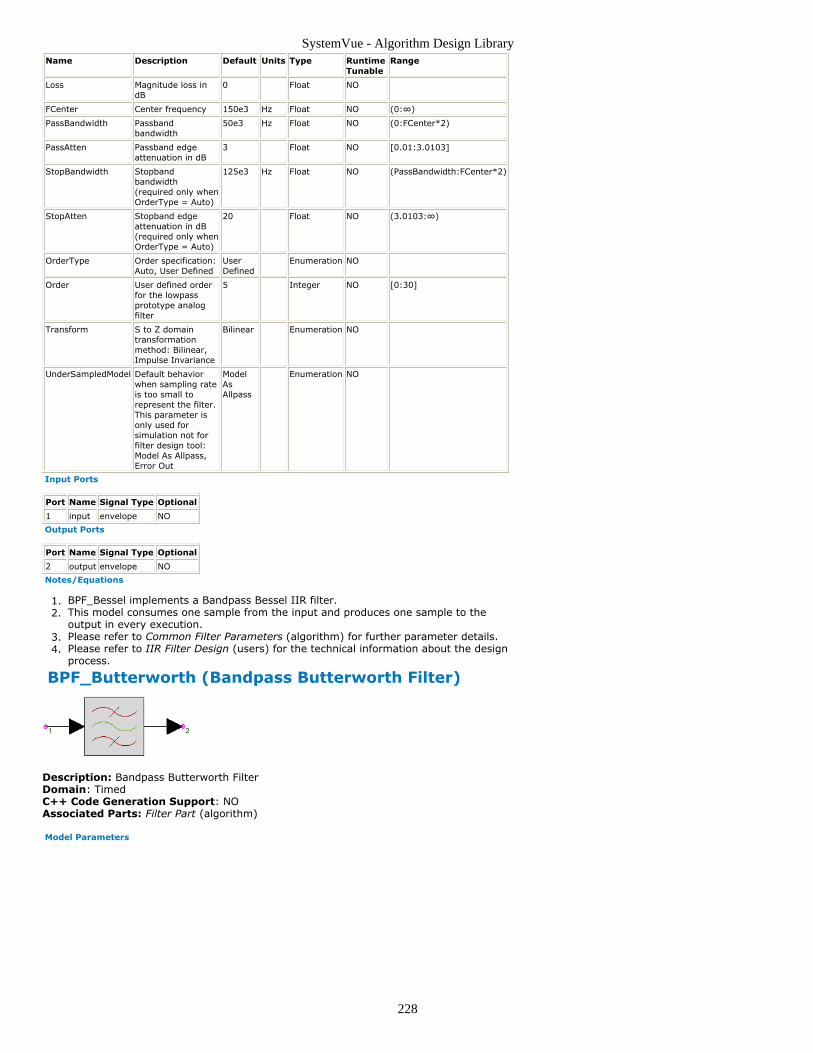
SystemVue - Algorithm Design Library
228
Name Description Default Units Type RuntimeTunable
Range
Loss Magnitude loss indB
0 Float NO
FCenter Center frequency 150e3 Hz Float NO (0:∞)
PassBandwidth Passbandbandwidth
50e3 Hz Float NO (0:FCenter*2)
PassAtten Passband edgeattenuation in dB
3 Float NO [0.01:3.0103]
StopBandwidth Stopbandbandwidth(required only whenOrderType = Auto)
125e3 Hz Float NO (PassBandwidth:FCenter*2)
StopAtten Stopband edgeattenuation in dB(required only whenOrderType = Auto)
20 Float NO (3.0103:∞)
OrderType Order specification:Auto, User Defined
UserDefined
Enumeration NO
Order User defined orderfor the lowpassprototype analogfilter
5 Integer NO [0:30]
Transform S to Z domaintransformationmethod: Bilinear,Impulse Invariance
Bilinear Enumeration NO
UnderSampledModel Default behaviorwhen sampling rateis too small torepresent the filter.This parameter isonly used forsimulation not forfilter design tool:Model As Allpass,Error Out
ModelAsAllpass
Enumeration NO
Input Ports
Port Name Signal Type Optional
1 input envelope NO
Output Ports
Port Name Signal Type Optional
2 output envelope NO
Notes/Equations
BPF_Bessel implements a Bandpass Bessel IIR filter.1.This model consumes one sample from the input and produces one sample to the2.output in every execution.Please refer to Common Filter Parameters (algorithm) for further parameter details.3.Please refer to IIR Filter Design (users) for the technical information about the design4.process.
BPF_Butterworth (Bandpass Butterworth Filter)
Description: Bandpass Butterworth FilterDomain: TimedC++ Code Generation Support: NOAssociated Parts: Filter Part (algorithm)
Model Parameters
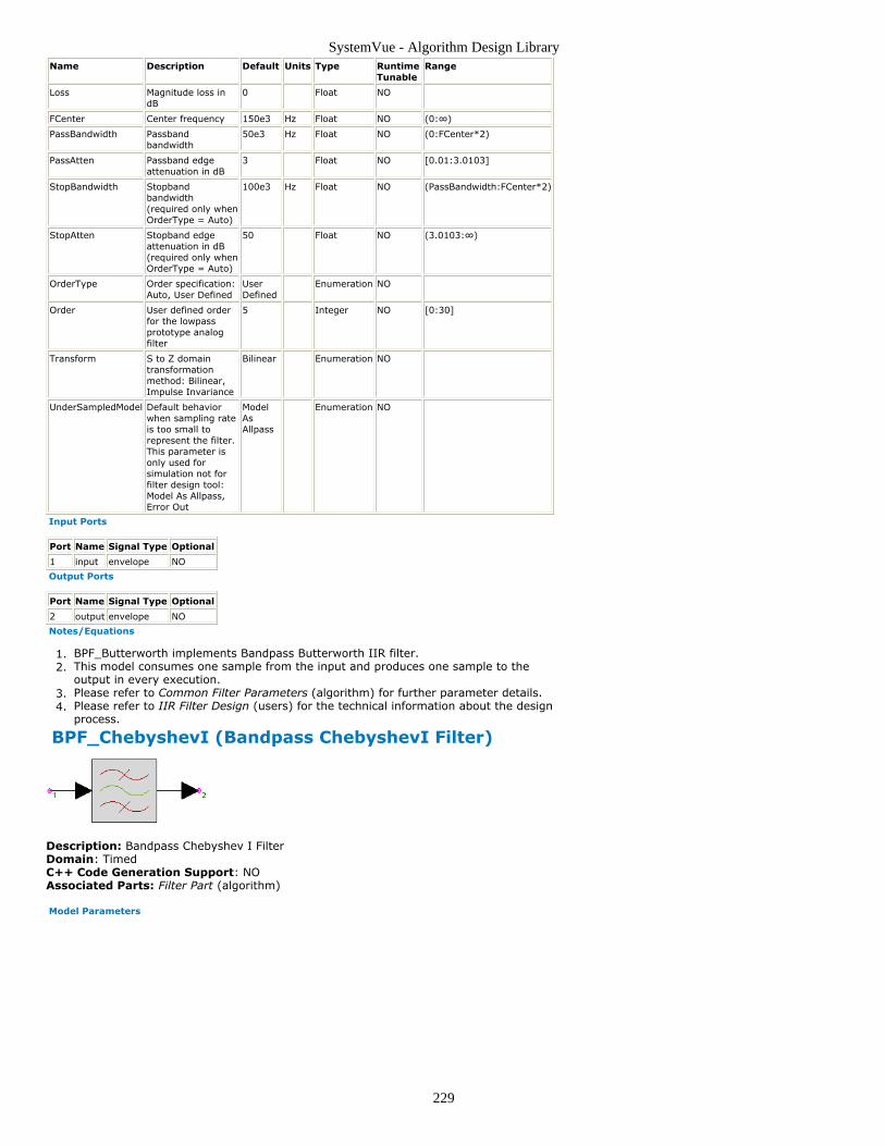
SystemVue - Algorithm Design Library
229
Name Description Default Units Type RuntimeTunable
Range
Loss Magnitude loss indB
0 Float NO
FCenter Center frequency 150e3 Hz Float NO (0:∞)
PassBandwidth Passbandbandwidth
50e3 Hz Float NO (0:FCenter*2)
PassAtten Passband edgeattenuation in dB
3 Float NO [0.01:3.0103]
StopBandwidth Stopbandbandwidth(required only whenOrderType = Auto)
100e3 Hz Float NO (PassBandwidth:FCenter*2)
StopAtten Stopband edgeattenuation in dB(required only whenOrderType = Auto)
50 Float NO (3.0103:∞)
OrderType Order specification:Auto, User Defined
UserDefined
Enumeration NO
Order User defined orderfor the lowpassprototype analogfilter
5 Integer NO [0:30]
Transform S to Z domaintransformationmethod: Bilinear,Impulse Invariance
Bilinear Enumeration NO
UnderSampledModel Default behaviorwhen sampling rateis too small torepresent the filter.This parameter isonly used forsimulation not forfilter design tool:Model As Allpass,Error Out
ModelAsAllpass
Enumeration NO
Input Ports
Port Name Signal Type Optional
1 input envelope NO
Output Ports
Port Name Signal Type Optional
2 output envelope NO
Notes/Equations
BPF_Butterworth implements Bandpass Butterworth IIR filter.1.This model consumes one sample from the input and produces one sample to the2.output in every execution.Please refer to Common Filter Parameters (algorithm) for further parameter details.3.Please refer to IIR Filter Design (users) for the technical information about the design4.process.
BPF_ChebyshevI (Bandpass ChebyshevI Filter)
Description: Bandpass Chebyshev I FilterDomain: TimedC++ Code Generation Support: NOAssociated Parts: Filter Part (algorithm)
Model Parameters

SystemVue - Algorithm Design Library
230
Name Description Default Units Type RuntimeTunable
Range
Loss Magnitude loss indB
0 Float NO
FCenter Center frequency 150e3 Hz Float NO (0:∞)
PassBandwidth Passbandbandwidth
50e3 Hz Float NO (0:FCenter*2)
PassRipple Passband ripple indB
1 Float NO [0.01:3.0103]
StopBandwidth Stopbandbandwidth(required only whenOrderType = Auto)
100e3 Hz Float NO (PassBandwidth:FCenter*2)
StopAtten Stopband edgeattenuation in dB(required only whenOrderType = Auto)
50 Float NO (3.0103:∞)
OrderType Order specification:Auto, User Defined
UserDefined
Enumeration NO
Order User defined orderfor the lowpassprototype analogfilter
5 Integer NO [0:30]
Transform S to Z domaintransformationmethod: Bilinear,Impulse Invariance
Bilinear Enumeration NO
UnderSampledModel Default behaviorwhen sampling rateis too small torepresent the filter.This parameter isonly used forsimulation not forfilter design tool:Model As Allpass,Error Out
ModelAsAllpass
Enumeration NO
Input Ports
Port Name Signal Type Optional
1 input envelope NO
Output Ports
Port Name Signal Type Optional
2 output envelope NO
Notes/Equations
BPF_ChebyshevI implements a Bandpass Chebyshev I IIR filter.1.This model consumes one sample from the input and produces one sample to the2.output in every execution.Please refer to Common Filter Parameters (algorithm) for further parameter details.3.Please refer to IIR Filter Design (users) for the technical information about the design4.process.
BPF_ChebyshevII (Bandpass ChebyshevII Filter)
Description: Bandpass Chebyshev II FilterDomain: TimedC++ Code Generation Support: NOAssociated Parts: Filter Part (algorithm)
Model Parameters

SystemVue - Algorithm Design Library
231
Name Description Default Units Type RuntimeTunable
Range
Loss Magnitude loss indB
0 Float NO
FCenter Center frequency 150e3 Hz Float NO (0:∞)
PassBandwidth Passbandbandwidth(required onlywhen OrderType =Auto)
50e3 Hz Float NO (0:FCenter*2)
PassAtten Passband edgeattenuation in dB(required onlywhen OrderType =Auto)
3 Float NO [0.01:3.0103]
StopBandwidth Stopbandbandwidth
100e3 Hz Float NO (PassBandwidth:FCenter*2)
StopRipple Stopband ripple indB
50 Float NO (3.0103:∞)
OrderType Order specification:Auto, User Defined
UserDefined
Enumeration NO
Order User defined orderfor the lowpassprototype analogfilter
5 Integer NO [0:30]
UnderSampledModel Default behaviorwhen sampling rateis too small torepresent the filter.This parameter isonly used forsimulation not forfilter design tool:Model As Allpass,Error Out
ModelAsAllpass
Enumeration NO
Input Ports
Port Name Signal Type Optional
1 input envelope NO
Output Ports
Port Name Signal Type Optional
2 output envelope NO
BPF_ChebyshevII implements a Bandpass Chebyshev II IIR filter.1.This model consumes one sample from the input and produces one sample to the2.output in every execution.Please refer to Common Filter Parameters (algorithm) for further parameter details.3.Please refer to IIR Filter Design (users) for the technical information about the design4.process.
BPF_Elliptic (Bandpass Elliptic Filter)
Description: Bandpass Elliptic FilterDomain: TimedC++ Code Generation Support: NOAssociated Parts: Filter Part (algorithm)
Model Parameters

SystemVue - Algorithm Design Library
232
Name Description Default Units Type RuntimeTunable
Range
Loss Magnitude loss indB
0 Float NO
FCenter Center frequency 150e3 Hz Float NO (0:∞)
PassBandwidth Passbandbandwidth
50e3 Hz Float NO (0:FCenter*2)
PassRipple Passband ripple indB
1 Float NO [0.01:3.0103]
StopBandwidth Stopbandbandwidth
100e3 Hz Float NO (PassBandwidth:FCenter*2)
StopRipple Stopband ripple indB (required onlywhen OrderType =Auto)
50 Float NO (3.0103:∞)
OrderType Order specification:Auto, User Defined
UserDefined
Enumeration NO
Order User defined orderfor the lowpassprototype analogfilter
5 Integer NO [0:30]
UnderSampledModel Default behaviorwhen sampling rateis too small torepresent the filter.This parameter isonly used forsimulation not forfilter design tool:Model As Allpass,Error Out
ModelAsAllpass
Enumeration NO
Input Ports
Port Name Signal Type Optional
1 input envelope NO
Output Ports
Port Name Signal Type Optional
2 output envelope NO
Notes/Equations
BPF_Elliptic implements a Bandpass Elliptic IIR filter.1.This model consumes one sample from the input and produces one sample to the2.output in every execution.Please refer to Common Filter Parameters (algorithm) for further parameter details.3.Please refer to IIR Filter Design (users) for the technical information about the design4.process.
BPF_Gaussian (Bandpass Gaussian Filter)
Description: Gaussian bandpass filterDomain: TimedC++ Code Generation Support: NOAssociated Parts: Filter Part (algorithm)
Model Parameters

SystemVue - Algorithm Design Library
233
Name Description Default Units Type RuntimeTunable
Range
Loss Magnitude loss in dB 0 Float NO [0:∞)
FCenter Center frequency 150e3 Hz Float NO (0:∞)
PassBandwidth Passband bandwidth 50e3 Hz Float NO (0:FCenter/2)
PassAtten Passband edge attenuationin dB
3 Float NO [0.01:3.0103]
LengthOption Filter length option (Auto:1.2 / 3db frequency): Auto,Number of Taps, ImpulseTime Duration
Auto Enumeration NO
Length Filter length (based onLengthOption, specifynumber of taps, or impulsetime duration; delay =length/2)
0 Float NO [0:∞)
Interpolation Interpolation (up sampling)factor
1 Integer NO [1:∞)
Decimation Decimation (down sampling)factor
1 Integer NO [1:∞)
DecimationPhase Decimation (down sampling)phase
0 Integer NO [0:_D_ecimation-1]
InterpolationScaling Gain adjustment forinterpolation: NO, YES
YES Enumeration NO
Input Ports
Port Name Signal Type Optional
1 input envelope NO
Output Ports
Port Name Signal Type Optional
2 output envelope NO
Notes/Equations
BPF_Gaussian implements a Bandpass Gaussian FIR filter.1.This model consumes Decimation number of samples from the input and produces2.Interpolation number of samples to the output in every execution.Please refer to Common Filter Parameters (algorithm) for further parameter details.3.Please refer to FIR Filter Design (users) for the technical information about the design4.process.The delay introduced by the filter is approximately equal to:5.
BPF_ParksMcClellan (Bandpass ParksMcClellanFilter)
Description: Bandpass linear phase FIR filter based on Parks-McClellan design methodDomain: TimedC++ Code Generation Support: NOAssociated Parts: Filter Part (algorithm)
Model Parameters

SystemVue - Algorithm Design Library
234
Name Description Default Units Type RuntimeTunable
Range
Loss Magnitude loss indB
0 Float NO [0:∞)
FCenter Center frequency 150e3 Hz Float NO (0:∞)
PassBandwidth Passbandbandwidth
50e3 Hz Float NO (0:FCenter*2)
PassRipple Passband ripple indB
1 Float NO [0.01:3.0103]
StopBandwidth Stopbandbandwidth
100e3 Hz Float NO (PassBandwidth:FCenter*2)
StopRipple Stopband ripple indB
30 Float NO [3.0103:∞]
MaximumOrder Maximum filterorder for Parks-McClellan filterdesign
300 Integer NO
Interpolation Interpolation (upsampling) factor
1 Integer NO [1:∞)
Decimation Decimation (downsampling) factor
1 Integer NO [1:∞)
DecimationPhase Decimation (downsampling) phase
0 Integer NO [0:_D_ecimation-1]
InterpolationScaling Gain adjustmentfor interpolation:NO, YES
YES Enumeration NO
Input Ports
Port Name Signal Type Optional
1 input envelope NO
Output Ports
Port Name Signal Type Optional
2 output envelope NO
Notes/Equations
BPF_ParksMcClellan implements a linear-phase Bandpass FIR filter using the Parks-1.McClellan design method.This model consumes Decimation number of samples from the input and produces2.Interpolation number of samples to the output in every execution.Please refer to Common Filter Parameters (algorithm) for further parameter details.3.Please refer to FIR Filter Design (users) for the technical information about the design4.process.
BPF_RaisedCosine (Bandpass Raised Cosine Filter)
Description: Raised cosine bandpass filterDomain: TimedC++ Code Generation Support: NOAssociated Parts: Filter Part (algorithm)
Model Parameters

SystemVue - Algorithm Design Library
235
Name Description Default Units Type RuntimeTunable
Range
Loss Magnitude loss in dB 0 Float NO [0:∞)
FCenter Center frequency 150e3 Hz Float NO (0:∞)
SymbolRate Symbol rate (passbandbandwidth = SymbolRate)
100e3 Hz Float NO (0:FCenter/2)
RollOff Roll-off factor (between 0and 1)
0.5 Float NO [0:1]
SquareRoot Square root option: NO,YES
NO Enumeration NO
PulseEqualization Pulse equalization option:NO, YES
NO Enumeration NO
LengthOption Filter length option (Auto:8 * symbol period): Auto,Number of Taps, Numberof Symbols, Impulse TimeDuration
Auto Enumeration NO
Length Filter length (length =2*delay) (based onLengthOption, specifynumber of taps, numberof symbols, or impulsetime duration)
0 Float NO [0:∞)
Window Window function:Rectangular, Bartlett,Hann, Hamming,Blackman, Flat Top
Rectangular Enumeration NO
Interpolation Interpolation (upsampling) factor
1 Integer NO [1:∞)
Decimation Decimation (downsampling) factor
1 Integer NO [1:∞)
DecimationPhase Decimation (downsampling) phase
0 Integer NO [0:_D_ecimation-1]
InterpolationScaling Gain adjustment forinterpolation: NO, YES
YES Enumeration NO
Input Ports
Port Name Signal Type Optional
1 input envelope NO
Output Ports
Port Name Signal Type Optional
2 output envelope NO
Notes/Equations
BPF_RaisedCosine implements a Bandpass Raised Cosine FIR filter.1.This model consumes Decimation number of samples from the input and produces2.Interpolation number of samples to the output in every execution.Please refer to Common Filter Parameters (algorithm) for further parameter details.3.Please refer to FIR Filter Design (users) for the technical information about the design4.process.
BPF_SynchronouslyTuned (BandpassSynchronouslyTuned Filter)
Description: Bandpass SynchronouslyTuned FilterDomain: TimedC++ Code Generation Support: NOAssociated Parts: Filter Part (algorithm)
Model Parameters

SystemVue - Algorithm Design Library
236
Name Description Default Units Type RuntimeTunable
Range
Loss Magnitude loss indB
0 Float NO
FCenter Center frequency 150e3 Hz Float NO (0:∞)
PassBandwidth Passbandbandwidth
50e3 Hz Float NO (0:FCenter*2)
PassAtten Passband edgeattenuation in dB
3 Float NO [0.01:3.0103]
StopBandwidth Stopbandbandwidth(required only whenOrderType = Auto)
150e3 Hz Float NO (PassBandwidth:FCenter*2)
StopAtten Stopband edgeattenuation in dB(required only whenOrderType = Auto)
20 Float NO (3.0103:∞)
OrderType Order specification:Auto, User Defined
UserDefined
Enumeration NO
Order User defined orderfor the lowpassprototype analogfilter
5 Integer NO [0:30]
Transform S to Z domaintransformationmethod: Bilinear,Impulse Invariance
Bilinear Enumeration NO
UnderSampledModel Default behaviorwhen sampling rateis too small torepresent the filter.This parameter isonly used forsimulation not forfilter design tool:Model As Allpass,Error Out
ModelAsAllpass
Enumeration NO
Input Ports
Port Name Signal Type Optional
1 input envelope NO
Output Ports
Port Name Signal Type Optional
2 output envelope NO
Notes/Equations
BPF_SynchronouslyTuned implements a Bandpass Synchronously Tuned IIR filter.1.This model consumes one sample from the input and produces one sample to the2.output in every execution.Please refer to Common Filter Parameters (algorithm) for further parameter details.3.Please refer to IIR Filter Design (users) for the technical information about the design4.process.
BPF_Window (Bandpass Window Filter)
Description: Bandpass window-based linear phase FIR filterDomain: TimedC++ Code Generation Support: NOAssociated Parts: Filter Part (algorithm)
Model Parameters

SystemVue - Algorithm Design Library
237
Name Description Default Units Type RuntimeTunable
Range
Window Window function:Rectangular,Bartlett, Hann,Hamming,Blackman, Flat Top,Generalized Cosine,Ready, Kaiser,BlackmanHarris
Kaiser Enumeration NO
Loss Magnitude loss in dB 0 Float NO [0:∞)
FCenter Center frequency 150e3 Hz Float NO (0:∞)
PassBandwidth Passband bandwidth 50e3 Hz Float NO (0:FCenter*2)
WindowParameter Window parameter 1 Floatingpoint array
NO
Order Filter order (numberof taps - 1)
30 Integer NO [0:512]
PassRipple Passband ripple indB
1 Float NO [0.01:3.0103]
StopBandwidth Stopband bandwidth(cutoff bandwidth =(PassBandwidth +StopBandwidth)/2)
100e3 Hz Float NO (PassBandwidth:FCenter*2)
StopAtten Stopband edgeattenuation in dB
20 Float NO [3.0103:∞]
Interpolation Interpolation (upsampling) factor
1 Integer NO [1:∞)
Decimation Decimation (downsampling) factor
1 Integer NO [1:∞)
DecimationPhase Decimation (downsampling) phase
0 Integer NO [0:_D_ecimation-1]
InterpolationScaling Gain adjustment forinterpolation: NO,YES
YES Enumeration NO
Input Ports
Port Name Signal Type Optional
1 input envelope NO
Output Ports
Port Name Signal Type Optional
2 output envelope NO
Notes/Equations
BPF_Window implements a linear-phase Bandpass FIR filter using the Window design1.method.This model consumes Decimation number of samples from the input and produces2.Interpolation number of samples to the output in every execution.Please refer to Common Filter Parameters (algorithm) for further parameter details.3.Please refer to FIR Filter Design (users) for the technical information about the design4.process.
BSF_Bessel (Bandstop Bessel Filter)
Description: Bandstop Bessel FilterDomain: TimedC++ Code Generation Support: NOAssociated Parts: Filter Part (algorithm)
Model Parameters

SystemVue - Algorithm Design Library
238
Name Description Default Units Type RuntimeTunable
Range
Loss Magnitude loss in dB 0 Float NO
FCenter Center frequency 150e3 Hz Float NO (0:∞)
PassBandwidth Passband bandwidth 200e3 Hz Float NO (StopBandwidth:FCenter*2)
PassAtten Passband edgeattenuation in dB
3 Float NO [0.01:3.0103]
StopBandwidth Stopband bandwidth(required only whenOrderType = Auto)
50e3 Hz Float NO (0:FCenter*2)
StopAtten Stopband edgeattenuation in dB(required only whenOrderType = Auto)
20 Float NO (3.0103:∞)
OrderType Order specification:Auto, User Defined
UserDefined
Enumeration NO
Order User defined order forthe lowpass prototypeanalog filter
5 Integer NO [0:30]
Input Ports
Port Name Signal Type Optional
1 input envelope NO
Output Ports
Port Name Signal Type Optional
2 output envelope NO
Notes/Equations
BSF_Bessel implements a Bandstop Bessel IIR filter.1.This model consumes one sample from the input and produces one sample to the2.output in every execution.Please refer to Common Filter Parameters (algorithm) for further parameter details.3.Please refer to IIR Filter Design (users) for the technical information about the design4.process.
BSF_Butterworth (Bandstop Butterworth Filter)
Description: Bandstop Butterworth FilterDomain: TimedC++ Code Generation Support: NOAssociated Parts: Filter Part (algorithm)
Model Parameters
Name Description Default Units Type RuntimeTunable
Range
Loss Magnitude loss in dB 0 Float NO
FCenter Center frequency 150e3 Hz Float NO (0:∞)
PassBandwidth Passband bandwidth 100e3 Hz Float NO (StopBandwidth:FCenter*2)
PassAtten Passband edgeattenuation in dB
3 Float NO [0.01:3.0103]
StopBandwidth Stopband bandwidth(required only whenOrderType = Auto)
50e3 Hz Float NO (0:FCenter*2)
StopAtten Stopband edgeattenuation in dB(required only whenOrderType = Auto)
50 Float NO (3.0103:∞)
OrderType Order specification:Auto, User Defined
UserDefined
Enumeration NO
Order User defined order forthe lowpass prototypeanalog filter
5 Integer NO [0:30]
Input Ports
Port Name Signal Type Optional
1 input envelope NO
Output Ports
Port Name Signal Type Optional
2 output envelope NO

SystemVue - Algorithm Design Library
239
Notes/Equations
BSF_Butterworth implements a Bandstop Butterworth IIR filter.1.This model consumes one sample from the input and produces one sample to the2.output in every execution.Please refer to Common Filter Parameters (algorithm) for further parameter details.3.Please refer to IIR Filter Design (users) for the technical information about the design4.process.
BSF_ChebyshevI (Bandstop ChebyshevI Filter)
Description: Bandstop Chebyshev I FilterDomain: TimedC++ Code Generation Support: NOAssociated Parts: Filter Part (algorithm)
Model Parameters
Name Description Default Units Type RuntimeTunable
Range
Loss Magnitude loss in dB 0 Float NO
FCenter Center frequency 150e3 Hz Float NO (0:∞)
PassBandwidth Passband bandwidth 100e3 Hz Float NO (StopBandwidth:FCenter*2)
PassRipple Passband ripple in dB 1 Float NO [0.01:3.0103]
StopBandwidth Stopband bandwidth(required only whenOrderType = Auto)
50e3 Hz Float NO (0:FCenter*2)
StopAtten Stopband edgeattenuation in dB(required only whenOrderType = Auto)
50 Float NO (3.0103:∞)
OrderType Order specification:Auto, User Defined
UserDefined
Enumeration NO
Order User defined order forthe lowpass prototypeanalog filter
5 Integer NO [0:30]
Input Ports
Port Name Signal Type Optional
1 input envelope NO
Output Ports
Port Name Signal Type Optional
2 output envelope NO
Notes/Equations
BSF_ChebyshevI implements a Bandstop Chebyshev I IIR filter.1.This model consumes one sample from the input and produces one sample to the2.output in every execution.Please refer to Common Filter Parameters (algorithm) for further parameter details.3.Please refer to IIR Filter Design (users) for the technical information about the design4.process.
BSF_ChebyshevII (Bandstop ChebyshevII Filter)
Description: Bandstop Chebyshev II FilterDomain: TimedC++ Code Generation Support: NOAssociated Parts: Filter Part (algorithm)
Model Parameters
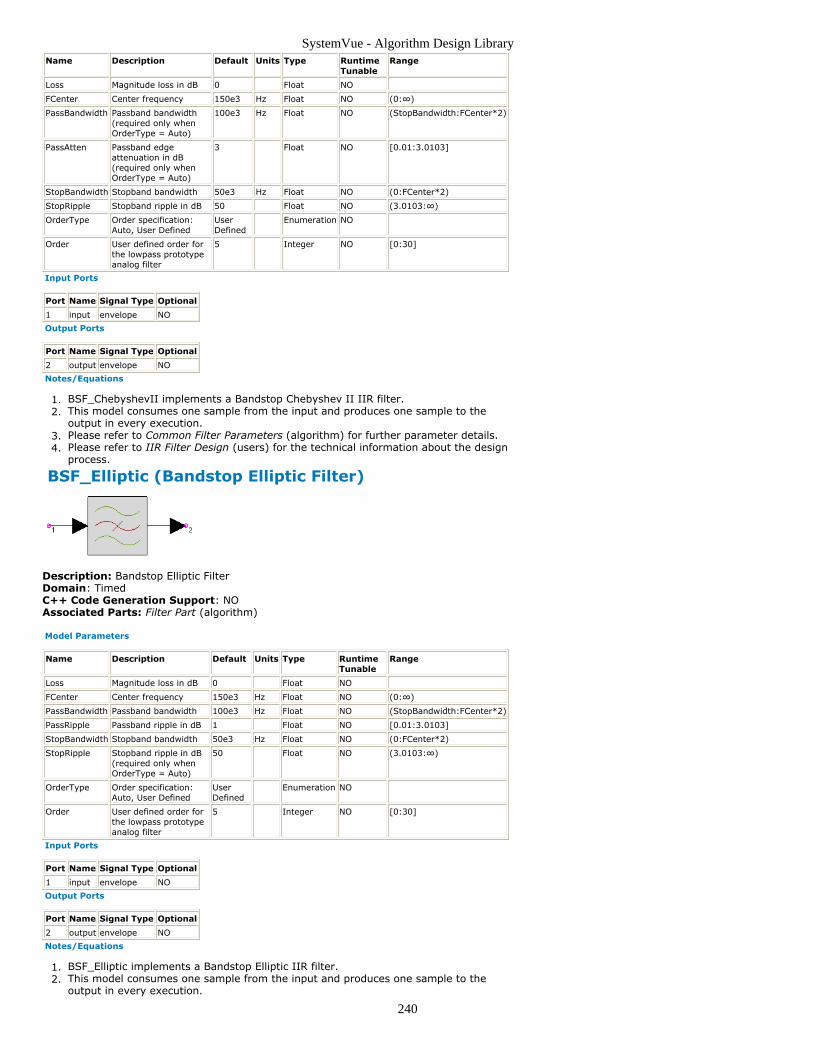
SystemVue - Algorithm Design Library
240
Name Description Default Units Type RuntimeTunable
Range
Loss Magnitude loss in dB 0 Float NO
FCenter Center frequency 150e3 Hz Float NO (0:∞)
PassBandwidth Passband bandwidth(required only whenOrderType = Auto)
100e3 Hz Float NO (StopBandwidth:FCenter*2)
PassAtten Passband edgeattenuation in dB(required only whenOrderType = Auto)
3 Float NO [0.01:3.0103]
StopBandwidth Stopband bandwidth 50e3 Hz Float NO (0:FCenter*2)
StopRipple Stopband ripple in dB 50 Float NO (3.0103:∞)
OrderType Order specification:Auto, User Defined
UserDefined
Enumeration NO
Order User defined order forthe lowpass prototypeanalog filter
5 Integer NO [0:30]
Input Ports
Port Name Signal Type Optional
1 input envelope NO
Output Ports
Port Name Signal Type Optional
2 output envelope NO
Notes/Equations
BSF_ChebyshevII implements a Bandstop Chebyshev II IIR filter.1.This model consumes one sample from the input and produces one sample to the2.output in every execution.Please refer to Common Filter Parameters (algorithm) for further parameter details.3.Please refer to IIR Filter Design (users) for the technical information about the design4.process.
BSF_Elliptic (Bandstop Elliptic Filter)
Description: Bandstop Elliptic FilterDomain: TimedC++ Code Generation Support: NOAssociated Parts: Filter Part (algorithm)
Model Parameters
Name Description Default Units Type RuntimeTunable
Range
Loss Magnitude loss in dB 0 Float NO
FCenter Center frequency 150e3 Hz Float NO (0:∞)
PassBandwidth Passband bandwidth 100e3 Hz Float NO (StopBandwidth:FCenter*2)
PassRipple Passband ripple in dB 1 Float NO [0.01:3.0103]
StopBandwidth Stopband bandwidth 50e3 Hz Float NO (0:FCenter*2)
StopRipple Stopband ripple in dB(required only whenOrderType = Auto)
50 Float NO (3.0103:∞)
OrderType Order specification:Auto, User Defined
UserDefined
Enumeration NO
Order User defined order forthe lowpass prototypeanalog filter
5 Integer NO [0:30]
Input Ports
Port Name Signal Type Optional
1 input envelope NO
Output Ports
Port Name Signal Type Optional
2 output envelope NO
Notes/Equations
BSF_Elliptic implements a Bandstop Elliptic IIR filter.1.This model consumes one sample from the input and produces one sample to the2.output in every execution.
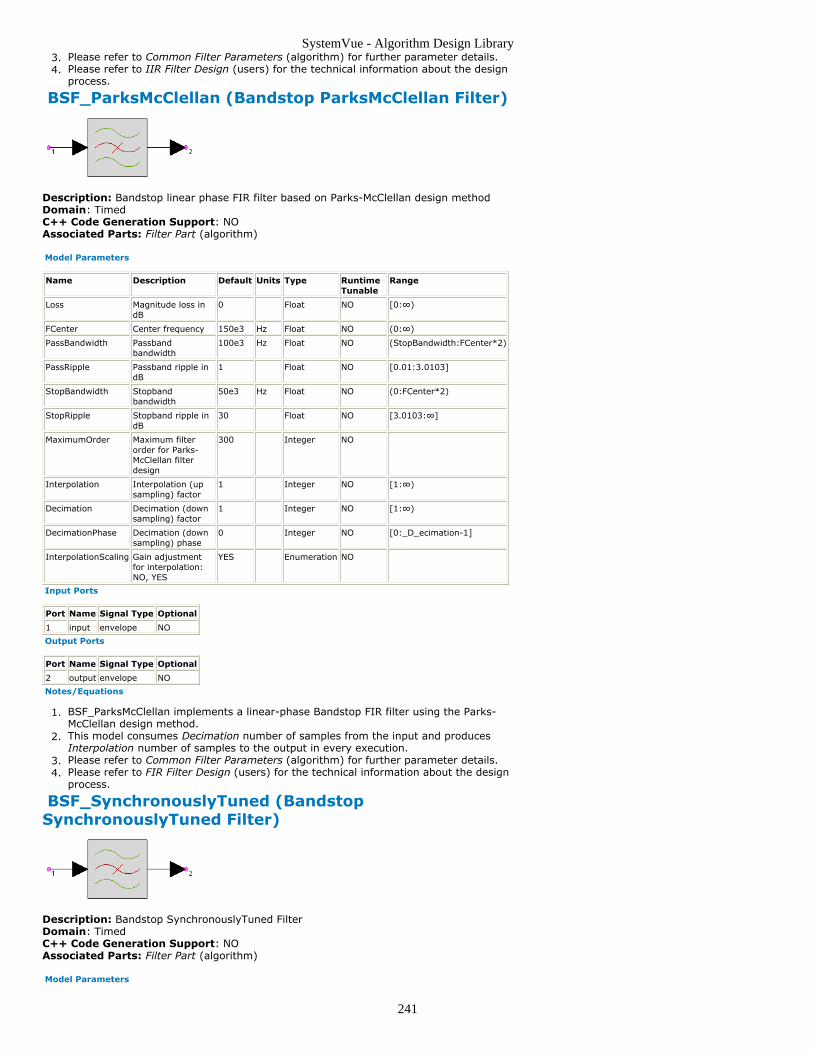
SystemVue - Algorithm Design Library
241
Please refer to Common Filter Parameters (algorithm) for further parameter details.3.Please refer to IIR Filter Design (users) for the technical information about the design4.process.
BSF_ParksMcClellan (Bandstop ParksMcClellan Filter)
Description: Bandstop linear phase FIR filter based on Parks-McClellan design methodDomain: TimedC++ Code Generation Support: NOAssociated Parts: Filter Part (algorithm)
Model Parameters
Name Description Default Units Type RuntimeTunable
Range
Loss Magnitude loss indB
0 Float NO [0:∞)
FCenter Center frequency 150e3 Hz Float NO (0:∞)
PassBandwidth Passbandbandwidth
100e3 Hz Float NO (StopBandwidth:FCenter*2)
PassRipple Passband ripple indB
1 Float NO [0.01:3.0103]
StopBandwidth Stopbandbandwidth
50e3 Hz Float NO (0:FCenter*2)
StopRipple Stopband ripple indB
30 Float NO [3.0103:∞]
MaximumOrder Maximum filterorder for Parks-McClellan filterdesign
300 Integer NO
Interpolation Interpolation (upsampling) factor
1 Integer NO [1:∞)
Decimation Decimation (downsampling) factor
1 Integer NO [1:∞)
DecimationPhase Decimation (downsampling) phase
0 Integer NO [0:_D_ecimation-1]
InterpolationScaling Gain adjustmentfor interpolation:NO, YES
YES Enumeration NO
Input Ports
Port Name Signal Type Optional
1 input envelope NO
Output Ports
Port Name Signal Type Optional
2 output envelope NO
Notes/Equations
BSF_ParksMcClellan implements a linear-phase Bandstop FIR filter using the Parks-1.McClellan design method.This model consumes Decimation number of samples from the input and produces2.Interpolation number of samples to the output in every execution.Please refer to Common Filter Parameters (algorithm) for further parameter details.3.Please refer to FIR Filter Design (users) for the technical information about the design4.process.
BSF_SynchronouslyTuned (BandstopSynchronouslyTuned Filter)
Description: Bandstop SynchronouslyTuned FilterDomain: TimedC++ Code Generation Support: NOAssociated Parts: Filter Part (algorithm)
Model Parameters

SystemVue - Algorithm Design Library
242
Name Description Default Units Type RuntimeTunable
Range
Loss Magnitude loss in dB 0 Float NO
FCenter Center frequency 150e3 Hz Float NO (0:∞)
PassBandwidth Passband bandwidth 200e3 Hz Float NO (StopBandwidth:FCenter*2)
PassAtten Passband edgeattenuation in dB
3 Float NO [0.01:3.0103]
StopBandwidth Stopband bandwidth(required only whenOrderType = Auto)
50e3 Hz Float NO (0:FCenter*2)
StopAtten Stopband edgeattenuation in dB(required only whenOrderType = Auto)
14 Float NO (3.0103:∞)
OrderType Order specification:Auto, User Defined
UserDefined
Enumeration NO
Order User defined order forthe lowpass prototypeanalog filter
5 Integer NO [0:30]
Input Ports
Port Name Signal Type Optional
1 input envelope NO
Output Ports
Port Name Signal Type Optional
2 output envelope NO
Notes/Equations
BSF_SynchronouslyTuned implements a Bandstop Synchronously Tuned IIR filter.1.This model consumes one sample from the input and produces one sample to the2.output in every execution.Please refer to Common Filter Parameters (algorithm) for further parameter details.3.Please refer to IIR Filter Design (users) for the technical information about the design4.process.
BSF_Window (Bandstop Window Filter)
Description: Bandstop window-based linear phase FIR filterDomain: TimedC++ Code Generation Support: NOAssociated Parts: Filter Part (algorithm)
Model Parameters

SystemVue - Algorithm Design Library
243
Name Description Default Units Type RuntimeTunable
Range
Window Window function:Rectangular, Bartlett, Hann,Hamming, Blackman, FlatTop, Generalized Cosine,Ready, Kaiser,BlackmanHarris
Kaiser Enumeration NO
Loss Magnitude loss in dB 0 Float NO [0:∞)
FCenter Center frequency 150e3 Hz Float NO (0:∞)
PassBandwidth Passband bandwidth 100e3 Hz Float NO (0:FCenter*2)
WindowParameter Window parameter 1 Floatingpoint array
NO
Order Filter order (set to evennumber)
30 Integer NO [0:512]
PassRipple Passband ripple in dB 1 Float NO [0.01:3.0103]
StopBandwidth Stopband bandwidth (cutoffbandwidth =(PassBandwidth +StopBandwidth)/2)
50e3 Hz Float NO (0:PassBandwidth)
StopAtten Stopband edge attenuationin dB
20 Float NO [3.0103:∞]
Interpolation Interpolation (up sampling)factor
1 Integer NO [1:∞)
Decimation Decimation (down sampling)factor
1 Integer NO [1:∞)
DecimationPhase Decimation (down sampling)phase
0 Integer NO [0:_D_ecimation-1]
InterpolationScaling Gain adjustment forinterpolation: NO, YES
YES Enumeration NO
Input Ports
Port Name Signal Type Optional
1 input envelope NO
Output Ports
Port Name Signal Type Optional
2 output envelope NO
Notes/Equations
BSF_Window implements a linear-phase Bandstop FIR filter using the Window design1.method.This model consumes Decimation number of samples from the input and produces2.Interpolation number of samples to the output in every execution.Please refer to Common Filter Parameters (algorithm) for further parameter details.3.Please refer to FIR Filter Design (users) for the technical information about the design4.process.
CustomFIR (Custom FIR Filter)
Description: Custom FIR filterDomain: TimedC++ Code Generation Support: NOAssociated Parts: Filter Part (algorithm)
Model Parameters
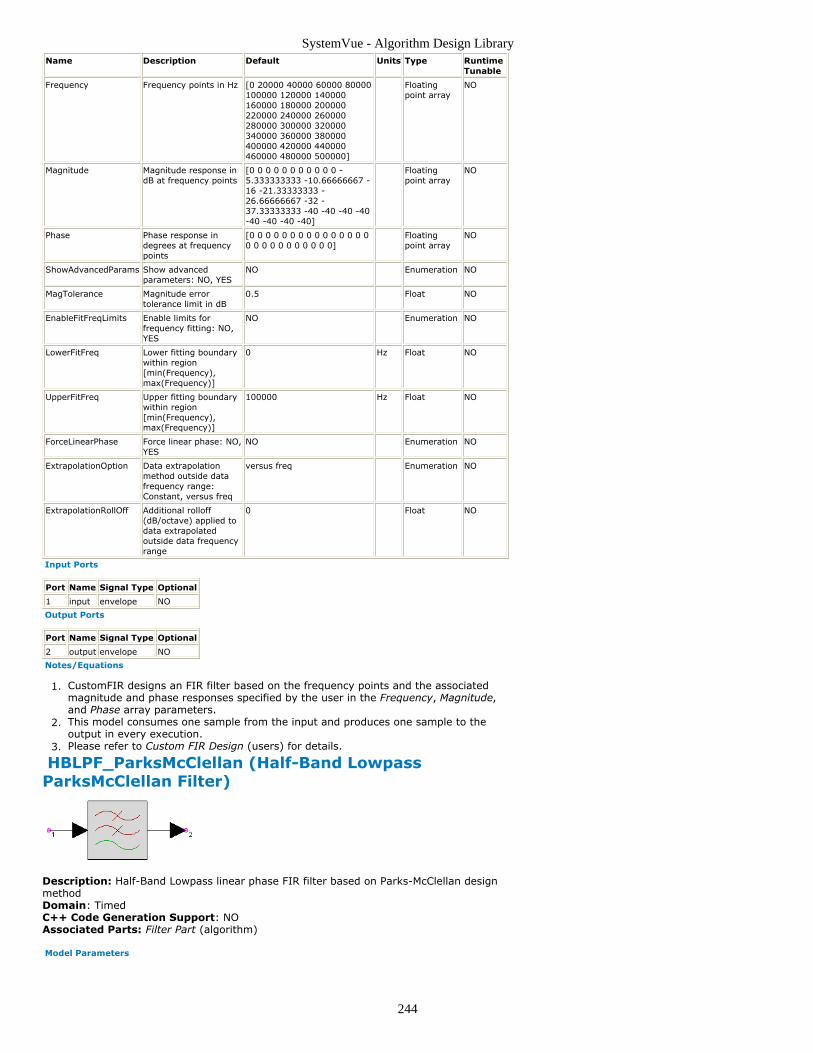
SystemVue - Algorithm Design Library
244
Name Description Default Units Type RuntimeTunable
Frequency Frequency points in Hz [0 20000 40000 60000 80000100000 120000 140000160000 180000 200000220000 240000 260000280000 300000 320000340000 360000 380000400000 420000 440000460000 480000 500000]
Floatingpoint array
NO
Magnitude Magnitude response indB at frequency points
[0 0 0 0 0 0 0 0 0 0 0 -5.333333333 -10.66666667 -16 -21.33333333 -26.66666667 -32 -37.33333333 -40 -40 -40 -40-40 -40 -40 -40]
Floatingpoint array
NO
Phase Phase response indegrees at frequencypoints
[0 0 0 0 0 0 0 0 0 0 0 0 0 0 00 0 0 0 0 0 0 0 0 0 0]
Floatingpoint array
NO
ShowAdvancedParams Show advancedparameters: NO, YES
NO Enumeration NO
MagTolerance Magnitude errortolerance limit in dB
0.5 Float NO
EnableFitFreqLimits Enable limits forfrequency fitting: NO,YES
NO Enumeration NO
LowerFitFreq Lower fitting boundarywithin region[min(Frequency),max(Frequency)]
0 Hz Float NO
UpperFitFreq Upper fitting boundarywithin region[min(Frequency),max(Frequency)]
100000 Hz Float NO
ForceLinearPhase Force linear phase: NO,YES
NO Enumeration NO
ExtrapolationOption Data extrapolationmethod outside datafrequency range:Constant, versus freq
versus freq Enumeration NO
ExtrapolationRollOff Additional rolloff(dB/octave) applied todata extrapolatedoutside data frequencyrange
0 Float NO
Input Ports
Port Name Signal Type Optional
1 input envelope NO
Output Ports
Port Name Signal Type Optional
2 output envelope NO
Notes/Equations
CustomFIR designs an FIR filter based on the frequency points and the associated1.magnitude and phase responses specified by the user in the Frequency, Magnitude,and Phase array parameters.This model consumes one sample from the input and produces one sample to the2.output in every execution.Please refer to Custom FIR Design (users) for details.3.
HBLPF_ParksMcClellan (Half-Band LowpassParksMcClellan Filter)
Description: Half-Band Lowpass linear phase FIR filter based on Parks-McClellan designmethodDomain: TimedC++ Code Generation Support: NOAssociated Parts: Filter Part (algorithm)
Model Parameters

SystemVue - Algorithm Design Library
245
Name Description Default Units Type RuntimeTunable
Range
Loss Magnitude loss in dB 0 Float NO [0:∞)
PassFreq Passband edge frequency 225e3 Hz Float NO (0:∞)
StopRipple Stopband ripple in dB 30 Float NO [3.0103:∞]
MaximumOrder Maximum filter order forParks-McClellan filterdesign
300 Integer NO
Interpolation Interpolation (upsampling) factor
1 Integer NO [1:∞)
Decimation Decimation (downsampling) factor
1 Integer NO [1:∞)
DecimationPhase Decimation (downsampling) phase
0 Integer NO [0:_D_ecimation-1]
InterpolationScaling Gain adjustment forinterpolation: NO, YES
YES Enumeration NO
Input Ports
Port Name Signal Type Optional
1 input envelope NO
Output Ports
Port Name Signal Type Optional
2 output envelope NO
Notes/Equations
HBLPF_ParksMcClellan implements a linear-phase Half-Band Lowpass FIR filter using1.the Parks-McClellan design method.This model consumes Decimation number of samples from the input and produces2.Interpolation number of samples to the output in every execution.Please refer to Common Filter Parameters (algorithm) for further parameter details.3.Please refer to FIR Filter Design (users) for the technical information about the design4.process.HBLPF_ParksMcClellan is a half-band version of LPF_ParksMcClellan (algorithm)5.where (PassFreq + StopFreq)/2 = SampleRate/4 and 0 < PassFreq < SampleRate/4.
HPF Bessel (Highpass Bessel Filter)
Description: Highpass Bessel FilterDomain: TimedC++ Code Generation Support: NOAssociated Parts: Filter Part (algorithm)
Model Parameters
Name Description Default Units Type RuntimeTunable
Range
Loss Magnitude loss in dB 0 Float NO
PassFreq Passband edge frequency 200e3 Hz Float NO (StopFreq:∞)
PassAtten Passband edge attenuation in dB 3 Float NO [0.01:3.0103]
StopFreq Stopband edge frequency (requiredonly when OrderType = Auto)
100e3 Hz Float NO (0:∞)
StopAtten Stopband edge attenuation in dB(required only when OrderType =Auto)
18 Float NO (3.0103:∞)
OrderType Order specification: Auto, UserDefined
UserDefined
Enumeration NO
Order User defined order for the lowpassprototype analog filter
5 Integer NO [0:30]
Input Ports
Port Name Signal Type Optional
1 input envelope NO
Output Ports
Port Name Signal Type Optional
2 output envelope NO
Notes/Equations
HPF_Bessel implements a Highpass Bessel IIR filter.1.This model consumes one sample from the input and produces one sample to the2.output in every execution.

SystemVue - Algorithm Design Library
246
Please refer to Common Filter Parameters (algorithm) for further parameter details.3.Please refer to IIR Filter Design (users) for the technical information about the design4.process.
HPF_Butterworth (Highpass Butterworth Filter)
Description: Highpass Butterworth FilterDomain: TimedC++ Code Generation Support: NOAssociated Parts: Filter Part (algorithm)
Model Parameters
Name Description Default Units Type RuntimeTunable
Range
Loss Magnitude loss in dB 0 Float NO
PassFreq Passband edge frequency 150e3 Hz Float NO (StopFreq:∞)
PassAtten Passband edge attenuation in dB 3 Float NO [0.01:3.0103]
StopFreq Stopband edge frequency (requiredonly when OrderType = Auto)
100e3 Hz Float NO (0:∞)
StopAtten Stopband edge attenuation in dB(required only when OrderType =Auto)
50 Float NO (3.0103:∞)
OrderType Order specification: Auto, UserDefined
UserDefined
Enumeration NO
Order User defined order for the lowpassprototype analog filter
5 Integer NO [0:30]
Input Ports
Port Name Signal Type Optional
1 input envelope NO
Output Ports
Port Name Signal Type Optional
2 output envelope NO
Notes/Equations
HPF_Butterworth implements a Highpass Butterworth IIR filter.1.This model consumes one sample from the input and produces one sample to the2.output in every execution.Please refer to Common Filter Parameters (algorithm) for further parameter details.3.Please refer to IIR Filter Design (users) for the technical information about the design4.process.
HPF_ChebyshevI (Highpass ChebyshevI Filter)
Description: Highpass Chebyshev I FilterDomain: TimedC++ Code Generation Support: NOAssociated Parts: Filter Part (algorithm)
Model Parameters
Name Description Default Units Type RuntimeTunable
Range
Loss Magnitude loss in dB 0 Float NO
PassFreq Passband edge frequency 150e3 Hz Float NO (StopFreq:∞)
PassRipple Passband ripple in dB 1 Float NO [0.01:3.0103]
StopFreq Stopband edge frequency (requiredonly when OrderType = Auto)
100e3 Hz Float NO (0:∞)
StopAtten Stopband edge attenuation in dB(required only when OrderType =Auto)
50 Float NO (3.0103:∞)
OrderType Order specification: Auto, UserDefined
UserDefined
Enumeration NO
Order User defined order for the lowpassprototype analog filter
5 Integer NO [0:30]

SystemVue - Algorithm Design Library
247
Input Ports
Port Name Signal Type Optional
1 input envelope NO
Output Ports
Port Name Signal Type Optional
2 output envelope NO
Notes/Equations
HPF_ChebyshevI implements a Highpass Chebyshev I IIR filter.1.This model consumes one sample from the input and produces one sample to the2.output in every execution.Please refer to Common Filter Parameters (algorithm) for further parameter details.3.Please refer to IIR Filter Design (users) for the technical information about the design4.process.
HPF_ChebyshevII (Highpass ChebyshevII Filter)
Description: Highpass Chebyshev II FilterDomain: TimedC++ Code Generation Support: NOAssociated Parts: Filter Part (algorithm)
Model Parameters
Name Description Default Units Type RuntimeTunable
Range
Loss Magnitude loss in dB 0 Float NO
PassFreq Passband edge frequency (requiredonly when OrderType = Auto)
150e3 Hz Float NO (StopFreq:∞)
PassAtten Passband edge attenuation in dB(required only when OrderType =Auto)
3 Float NO [0.01:3.0103]
StopFreq Stopband edge frequency 100e3 Hz Float NO (0:∞)
StopRipple Stopband ripple in dB 50 Float NO (3.0103:∞)
OrderType Order specification: Auto, UserDefined
UserDefined
Enumeration NO
Order User defined order for the lowpassprototype analog filter
5 Integer NO [0:30]
Input Ports
Port Name Signal Type Optional
1 input envelope NO
Output Ports
Port Name Signal Type Optional
2 output envelope NO
Notes/Equations
HPF_ChebyshevII implements a Highpass Chebyshev II IIR filter.1.This model consumes one sample from the input and produces one sample to the2.output in every execution.Please refer to Common Filter Parameters (algorithm) for further parameter details.3.Please refer to IIR Filter Design (users) for the technical information about the design4.process.
HPF_Elliptic (Highpass Elliptic Filter)
Description: Highpass Elliptic FilterDomain: TimedC++ Code Generation Support: NOAssociated Parts: Filter Part (algorithm)
Model Parameters

SystemVue - Algorithm Design Library
248
Name Description Default Units Type RuntimeTunable
Range
Loss Magnitude loss in dB 0 Float NO
PassFreq Passband edge frequency 150e3 Hz Float NO (StopFreq:∞)
PassRipple Passband ripple in dB 1 Float NO [0.01:3.0103]
StopFreq Stopband edge frequency 100e3 Hz Float NO (0:∞)
StopRipple Stopband ripple in dB (required onlywhen OrderType = Auto)
50 Float NO (3.0103:∞)
OrderType Order specification: Auto, UserDefined
UserDefined
Enumeration NO
Order User defined order for the lowpassprototype analog filter
5 Integer NO [0:30]
Input Ports
Port Name Signal Type Optional
1 input envelope NO
Output Ports
Port Name Signal Type Optional
2 output envelope NO
Notes/Equations
HPF_Elliptic implements a Highpass Elliptic IIR filter.1.This model consumes one sample from the input and produces one sample to the2.output in every execution.Please refer to Common Filter Parameters (algorithm) for further parameter details.3.Please refer to IIR Filter Design (users) for the technical information about the design4.process.
HPF_ParksMcClellan (Highpass ParksMcClellan Filter)
Description: Highpass linear phase FIR filter based on Parks-McClellan design methodDomain: TimedC++ Code Generation Support: NOAssociated Parts: Filter Part (algorithm)
Model Parameters
Name Description Default Units Type RuntimeTunable
Range
Loss Magnitude loss in dB 0 Float NO [0:∞)
PassFreq Passband edge frequency 150e3 Hz Float NO (0:∞)
PassRipple Passband ripple in dB 1 Float NO [0.01:3.0103]
StopFreq Stopband edge frequency 100e3 Hz Float NO (PassFreq:∞)
StopRipple Stopband ripple in dB 30 Float NO [3.0103:∞]
MaximumOrder Maximum filter order forParks-McClellan filterdesign
300 Integer NO
Interpolation Interpolation (upsampling) factor
1 Integer NO [1:∞)
Decimation Decimation (downsampling) factor
1 Integer NO [1:∞)
DecimationPhase Decimation (downsampling) phase
0 Integer NO [0:_D_ecimation-1]
InterpolationScaling Gain adjustment forinterpolation: NO, YES
YES Enumeration NO
Input Ports
Port Name Signal Type Optional
1 input envelope NO
Output Ports
Port Name Signal Type Optional
2 output envelope NO
Notes/Equations
HPF_ParksMcClellan implements a linear-phase Highpass FIR filter using the Parks-1.McClellan design method.This model consumes Decimation number of samples from the input and produces2.Interpolation number of samples to the output in every execution.Please refer to Common Filter Parameters (algorithm) for further parameter details.3.

SystemVue - Algorithm Design Library
249
Please refer to FIR Filter Design (users) for the technical information about the design4.process.
HPF_SynchronouslyTuned (HighpassSynchronouslyTuned Filter)
Description: Highpass Synchronously Tuned FilterDomain: TimedC++ Code Generation Support: NOAssociated Parts: Filter Part (algorithm)
Model Parameters
Name Description Default Units Type RuntimeTunable
Range
Loss Magnitude loss in dB 0 Float NO
PassFreq Passband edge frequency 250e3 Hz Float NO (StopFreq:∞)
PassAtten Passband edge attenuation in dB 3 Float NO [0.01:3.0103]
StopFreq Stopband edge frequency (requiredonly when OrderType = Auto)
100e3 Hz Float NO (0:∞)
StopAtten Stopband edge attenuation in dB(required only when OrderType =Auto)
20 Float NO (3.0103:∞)
OrderType Order specification: Auto, UserDefined
UserDefined
Enumeration NO
Order User defined order for the lowpassprototype analog filter
5 Integer NO [0:30]
Input Ports
Port Name Signal Type Optional
1 input envelope NO
Output Ports
Port Name Signal Type Optional
2 output envelope NO
Notes/Equations
HPF_SynchronouslyTuned implements a Highpass Synchronously Tuned IIR filter.1.This model consumes one sample from the input and produces one sample to the2.output in every execution.Please refer to Common Filter Parameters (algorithm) for further parameter details.3.Please refer to IIR Filter Design (users) for the technical information about the design4.process.
HPF_Window (Highpass Window Filter)
Description: Highpass window-based linear phase FIR filterDomain: TimedC++ Code Generation Support: NOAssociated Parts: Filter Part (algorithm)
Model Parameters

SystemVue - Algorithm Design Library
250
Name Description Default Units Type RuntimeTunable
Range
Window Window function:Rectangular, Bartlett, Hann,Hamming, Blackman, FlatTop, Generalized Cosine,Ready, Kaiser,BlackmanHarris
Kaiser Enumeration NO
Loss Magnitude loss in dB 0 Float NO [0:∞)
PassFreq Passband edge frequency 150e3 Hz Float NO (0:∞)
WindowParameter Window parameter 1 Floatingpoint array
NO
Order Filter order (number of taps- 1)
30 Integer NO [0:512]
PassRipple Passband ripple in dB 1 Float NO [0.01:3.0103]
StopFreq Stopband edge frequency(cutoff frequency =(PassFreq + StopFreq)/2)
100e3 Hz Float NO (0:PassFreq)
StopAtten Stopband edge attenuationin dB
20 Float NO [3.0103:∞]
Interpolation Interpolation (up sampling)factor
1 Integer NO [1:∞)
Decimation Decimation (down sampling)factor
1 Integer NO [1:∞)
DecimationPhase Decimation (down sampling)phase
0 Integer NO [0:_D_ecimation-1]
InterpolationScaling Gain adjustment forinterpolation: NO, YES
YES Enumeration NO
Input Ports
Port Name Signal Type Optional
1 input envelope NO
Output Ports
Port Name Signal Type Optional
2 output envelope NO
Notes/Equations
HPF_Window implements a linear-phase Highpass FIR filter using the Window design1.method.This model consumes Decimation number of samples from the input and produces2.Interpolation number of samples to the output in every execution.Please refer to Common Filter Parameters (algorithm) for further parameter details.3.Please refer to FIR Filter Design (users) for the technical information about the design4.process.
LPF_Bessel (Lowpass Bessel Filter)
Description: Lowpass Bessel FilterDomain: TimedC++ Code Generation Support: NOAssociated Parts: Filter Part (algorithm)
Model Parameters

SystemVue - Algorithm Design Library
251
Name Description Default Units Type RuntimeTunable
Range
Loss Magnitude loss in dB 0 Float NO
PassFreq Passband edge frequency 100e3 Hz Float NO (0:∞)
PassAtten Passband edge attenuation indB
3 Float NO [0.01:3.0103]
StopFreq Stopband edge frequency(required only when OrderType= Auto)
200e3 Hz Float NO (PassFreq:∞)
StopAtten Stopband edge attenuation indB (required only whenOrderType = Auto)
18 Float NO (3.0103:∞)
OrderType Order specification: Auto, UserDefined
UserDefined
Enumeration NO
Order User defined order for thelowpass prototype analog filter
5 Integer NO [0:30]
Transform S to Z domain transformationmethod: Bilinear, ImpulseInvariance
Bilinear Enumeration NO
UnderSampledModel Default behavior when samplingrate is too small to representthe filter. This parameter is onlyused for simulation not for filterdesign tool: Model As Allpass,Error Out
Model AsAllpass
Enumeration NO
Input Ports
Port Name Signal Type Optional
1 input envelope NO
Output Ports
Port Name Signal Type Optional
2 output envelope NO
Notes/Equations
LPF_Bessel implements a Lowpass Bessel IIR filter.1.This model consumes one sample from the input and produces one sample to the2.output in every execution.Please refer to Common Filter Parameters (algorithm) for further parameter details.3.Please refer to IIR Filter Design (users) for the technical information about the design4.process.
LPF_Butterworth (Lowpass Butterworth Filter)
Description: Lowpass Butterworth FilterDomain: TimedC++ Code Generation Support: NOAssociated Parts: Filter Part (algorithm)
Model Parameters

SystemVue - Algorithm Design Library
252
Name Description Default Units Type RuntimeTunable
Range
Loss Magnitude loss in dB 0 Float NO
PassFreq Passband edge frequency 100e3 Hz Float NO (0:∞)
PassAtten Passband edge attenuation indB
3 Float NO [0.01:3.0103]
StopFreq Stopband edge frequency(required only when OrderType= Auto)
150e3 Hz Float NO (PassFreq:∞)
StopAtten Stopband edge attenuation indB (required only whenOrderType = Auto)
50 Float NO (3.0103:∞)
OrderType Order specification: Auto, UserDefined
UserDefined
Enumeration NO
Order User defined order for thelowpass prototype analog filter
5 Integer NO [0:30]
Transform S to Z domain transformationmethod: Bilinear, ImpulseInvariance
Bilinear Enumeration NO
UnderSampledModel Default behavior when samplingrate is too small to representthe filter. This parameter is onlyused for simulation not for filterdesign tool: Model As Allpass,Error Out
Model AsAllpass
Enumeration NO
Input Ports
Port Name Signal Type Optional
1 input envelope NO
Output Ports
Port Name Signal Type Optional
2 output envelope NO
Notes/Equations
LPF_Butterworth implements a Lowpass Butterworth IIR filter.1.This model consumes one sample from the input and produces one sample to the2.output in every execution.Please refer to Common Filter Parameters (algorithm) for further parameter details.3.Please refer to IIR Filter Design (users) for the technical information about the design4.process.
LPF_ChebyshevI (Lowpass ChebyshevI Filter)
Description: Lowpass Chebyshev I FilterDomain: TimedC++ Code Generation Support: NOAssociated Parts: Filter Part (algorithm)
Model Parameters
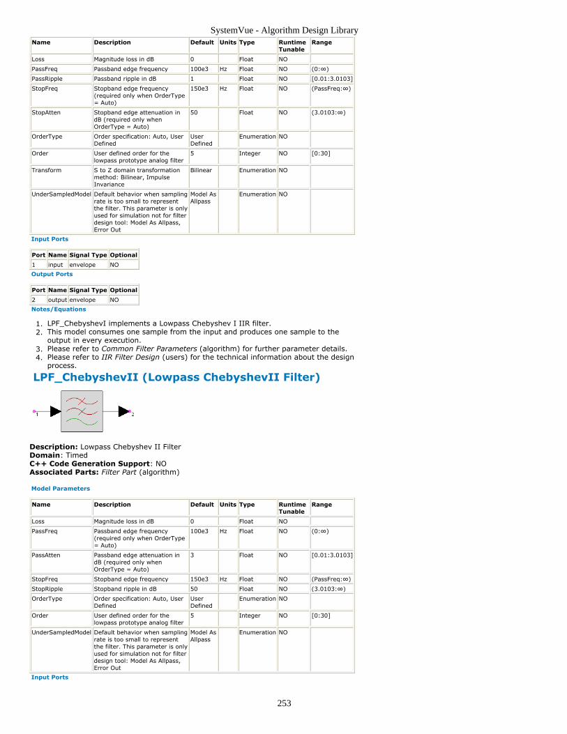
SystemVue - Algorithm Design Library
253
Name Description Default Units Type RuntimeTunable
Range
Loss Magnitude loss in dB 0 Float NO
PassFreq Passband edge frequency 100e3 Hz Float NO (0:∞)
PassRipple Passband ripple in dB 1 Float NO [0.01:3.0103]
StopFreq Stopband edge frequency(required only when OrderType= Auto)
150e3 Hz Float NO (PassFreq:∞)
StopAtten Stopband edge attenuation indB (required only whenOrderType = Auto)
50 Float NO (3.0103:∞)
OrderType Order specification: Auto, UserDefined
UserDefined
Enumeration NO
Order User defined order for thelowpass prototype analog filter
5 Integer NO [0:30]
Transform S to Z domain transformationmethod: Bilinear, ImpulseInvariance
Bilinear Enumeration NO
UnderSampledModel Default behavior when samplingrate is too small to representthe filter. This parameter is onlyused for simulation not for filterdesign tool: Model As Allpass,Error Out
Model AsAllpass
Enumeration NO
Input Ports
Port Name Signal Type Optional
1 input envelope NO
Output Ports
Port Name Signal Type Optional
2 output envelope NO
Notes/Equations
LPF_ChebyshevI implements a Lowpass Chebyshev I IIR filter.1.This model consumes one sample from the input and produces one sample to the2.output in every execution.Please refer to Common Filter Parameters (algorithm) for further parameter details.3.Please refer to IIR Filter Design (users) for the technical information about the design4.process.
LPF_ChebyshevII (Lowpass ChebyshevII Filter)
Description: Lowpass Chebyshev II FilterDomain: TimedC++ Code Generation Support: NOAssociated Parts: Filter Part (algorithm)
Model Parameters
Name Description Default Units Type RuntimeTunable
Range
Loss Magnitude loss in dB 0 Float NO
PassFreq Passband edge frequency(required only when OrderType= Auto)
100e3 Hz Float NO (0:∞)
PassAtten Passband edge attenuation indB (required only whenOrderType = Auto)
3 Float NO [0.01:3.0103]
StopFreq Stopband edge frequency 150e3 Hz Float NO (PassFreq:∞)
StopRipple Stopband ripple in dB 50 Float NO (3.0103:∞)
OrderType Order specification: Auto, UserDefined
UserDefined
Enumeration NO
Order User defined order for thelowpass prototype analog filter
5 Integer NO [0:30]
UnderSampledModel Default behavior when samplingrate is too small to representthe filter. This parameter is onlyused for simulation not for filterdesign tool: Model As Allpass,Error Out
Model AsAllpass
Enumeration NO
Input Ports
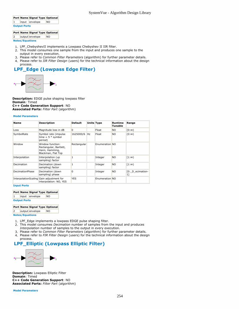
SystemVue - Algorithm Design Library
254
Port Name Signal Type Optional
1 input envelope NO
Output Ports
Port Name Signal Type Optional
2 output envelope NO
Notes/Equations
LPF_ChebyshevII implements a Lowpass Chebyshev II IIR filter.1.This model consumes one sample from the input and produces one sample to the2.output in every execution.Please refer to Common Filter Parameters (algorithm) for further parameter details.3.Please refer to IIR Filter Design (users) for the technical information about the design4.process.
LPF_Edge (Lowpass Edge Filter)
Description: EDGE pulse shaping lowpass filterDomain: TimedC++ Code Generation Support: NOAssociated Parts: Filter Part (algorithm)
Model Parameters
Name Description Default Units Type RuntimeTunable
Range
Loss Magnitude loss in dB 0 Float NO [0:∞)
SymbolRate Symbol rate (impulsetime = 5 * symbolperiod)
1625000/6 Hz Float NO (0:∞)
Window Window function:Rectangular, Bartlett,Hann, Hamming,Blackman, Flat Top
Rectangular Enumeration NO
Interpolation Interpolation (upsampling) factor
1 Integer NO [1:∞)
Decimation Decimation (downsampling) factor
1 Integer NO [1:∞)
DecimationPhase Decimation (downsampling) phase
0 Integer NO [0:_D_ecimation-1]
InterpolationScaling Gain adjustment forinterpolation: NO, YES
YES Enumeration NO
Input Ports
Port Name Signal Type Optional
1 input envelope NO
Output Ports
Port Name Signal Type Optional
2 output envelope NO
Notes/Equations
LPF_Edge implements a lowpass EDGE pulse shaping filter.1.This model consumes Decimation number of samples from the input and produces2.Interpolation number of samples to the output in every execution.Please refer to Common Filter Parameters (algorithm) for further parameter details.3.Please refer to FIR Filter Design (users) for the technical information about the design4.process.
LPF_Elliptic (Lowpass Elliptic Filter)
Description: Lowpass Elliptic FilterDomain: TimedC++ Code Generation Support: NOAssociated Parts: Filter Part (algorithm)
Model Parameters

SystemVue - Algorithm Design Library
255
Name Description Default Units Type RuntimeTunable
Range
Loss Magnitude loss in dB 0 Float NO
PassFreq Passband edge frequency 100e3 Hz Float NO (0:∞)
PassRipple Passband ripple in dB 1 Float NO [0.01:3.0103]
StopFreq Stopband edge frequency 150e3 Hz Float NO (PassFreq:∞)
StopRipple Stopband ripple in dB (requiredonly when OrderType = Auto)
50 Float NO (3.0103:∞)
OrderType Order specification: Auto, UserDefined
UserDefined
Enumeration NO
Order User defined order for thelowpass prototype analog filter
5 Integer NO [0:30]
UnderSampledModel Default behavior when samplingrate is too small to representthe filter. This parameter is onlyused for simulation not for filterdesign tool: Model As Allpass,Error Out
Model AsAllpass
Enumeration NO
Input Ports
Port Name Signal Type Optional
1 input envelope NO
Output Ports
Port Name Signal Type Optional
2 output envelope NO
Notes/Equations
LPF_Elliptic implements a Lowpass Elliptic IIR filter.1.This model consumes one sample from the input and produces one sample to the2.output in every execution.Please refer to Common Filter Parameters (algorithm) for further parameter details.3.Please refer to IIR Filter Design (users) for the technical information about the design4.process.
LPF_Gaussian (Lowpass Gaussian Filter)
Description: Gaussian lowpass filterDomain: TimedC++ Code Generation Support: NOAssociated Parts: Filter Part (algorithm)
Model Parameters
Name Description Default Units Type RuntimeTunable
Range
Loss Magnitude loss in dB 0 Float NO [0:∞)
PassFreq Passband edge frequency 100e3 Hz Float NO (0:∞)
PassAtten Passband edge attenuationin dB
3 Float NO [0.01:3.0103]
LengthOption Filter length option (Auto:1.2 / 3db frequency): Auto,Number of Taps, ImpulseTime Duration
Auto Enumeration NO
Length Filter length (based onLengthOption, specifynumber of taps, or impulsetime duration; delay =length/2)
0 Float NO [0:∞)
Interpolation Interpolation (up sampling)factor
1 Integer NO [1:∞)
Decimation Decimation (down sampling)factor
1 Integer NO [1:∞)
DecimationPhase Decimation (down sampling)phase
0 Integer NO [0:_D_ecimation-1]
InterpolationScaling Gain adjustment forinterpolation: NO, YES
YES Enumeration NO
Input Ports
Port Name Signal Type Optional
1 input envelope NO
Output Ports

SystemVue - Algorithm Design Library
256
Port Name Signal Type Optional
2 output envelope NO
Notes/Equations
The delay introduced by the filter is approximately equal to:1.
LPF_ParksMcClellan (Lowpass ParksMcClellan Filter)
Description: Lowpass linear phase FIR filter based on Parks-McClellan design methodDomain: TimedC++ Code Generation Support: NOAssociated Parts: Filter Part (algorithm)
Model Parameters
Name Description Default Units Type RuntimeTunable
Range
Loss Magnitude loss in dB 0 Float NO [0:∞)
PassFreq Passband edge frequency 100e3 Hz Float NO (0:∞)
PassRipple Passband ripple in dB 1 Float NO [0.01:3.0103]
StopFreq Stopband edge frequency 150e3 Hz Float NO (PassFreq:∞)
StopRipple Stopband ripple in dB 30 Float NO [3.0103:∞]
MaximumOrder Maximum filter order forParks-McClellan filterdesign
300 Integer NO
Interpolation Interpolation (upsampling) factor
1 Integer NO [1:∞)
Decimation Decimation (downsampling) factor
1 Integer NO [1:∞)
DecimationPhase Decimation (downsampling) phase
0 Integer NO [0:_D_ecimation-1]
InterpolationScaling Gain adjustment forinterpolation: NO, YES
YES Enumeration NO
Input Ports
Port Name Signal Type Optional
1 input envelope NO
Output Ports
Port Name Signal Type Optional
2 output envelope NO
Notes/Equations
LPF_ParksMcClellan implements a linear-phase Lowpass FIR filter using the Parks-1.McClellan design method.This model consumes Decimation number of samples from the input and produces2.Interpolation number of samples to the output in every execution.Please refer to Common Filter Parameters (algorithm) for further parameter details.3.Please refer to FIR Filter Design (users) for the technical information about the design4.process.
LPF_RaisedCosine (Lowpass Raised Cosine Filter)
Description: Raised cosine lowpass filterDomain: TimedC++ Code Generation Support: NOAssociated Parts: Filter Part (algorithm)
Model Parameters

SystemVue - Algorithm Design Library
257
Name Description Default Units Type RuntimeTunable
Range
Loss Magnitude loss in dB 0 Float NO [0:∞)
SymbolRate Symbol rate (passbandedge frequency =SymbolRate/2)
100e3 Hz Float NO (0:∞)
RollOff Roll-off factor (between 0and 1)
0.5 Float NO [0:1]
SquareRoot Square root option: NO,YES
NO Enumeration NO
PulseEqualization Pulse equalization option:NO, YES
NO Enumeration NO
LengthOption Filter length option (Auto:8 * symbol period): Auto,Number of Taps, Numberof Symbols, Impulse TimeDuration
Auto Enumeration NO
Length Filter length (length =2*delay) (based onLengthOption, specifynumber of taps, numberof symbols, or impulsetime duration)
0 Float NO [0:∞)
Window Window function:Rectangular, Bartlett,Hann, Hamming,Blackman, Flat Top
Rectangular Enumeration NO
Interpolation Interpolation (upsampling) factor
1 Integer NO [1:∞)
Decimation Decimation (downsampling) factor
1 Integer NO [1:∞)
DecimationPhase Decimation (downsampling) phase
0 Integer NO [0:_D_ecimation-1]
InterpolationScaling Gain adjustment forinterpolation: NO, YES
YES Enumeration NO
Input Ports
Port Name Signal Type Optional
1 input envelope NO
Output Ports
Port Name Signal Type Optional
2 output envelope NO
Notes/Equations
LPF_RaisedCosine implements a Lowpass Raised Cosine FIR filter.1.This model consumes Decimation number of samples from the input and produces2.Interpolation number of samples to the output in every execution.Please refer to Common Filter Parameters (algorithm) for further parameter details.3.Please refer to FIR Filter Design (users) for the technical information about the design4.process.
LPF_SynchronouslyTuned (LowpassSynchronouslyTuned Filter)
Description: Lowpass Synchronously Tuned FilterDomain: TimedC++ Code Generation Support: NOAssociated Parts: Filter Part (algorithm)
Model Parameters

SystemVue - Algorithm Design Library
258
Name Description Default Units Type RuntimeTunable
Range
Loss Magnitude loss in dB 0 Float NO
PassFreq Passband edge frequency 100e3 Hz Float NO (0:∞)
PassAtten Passband edge attenuation indB
3 Float NO [0.01:3.0103]
StopFreq Stopband edge frequency(required only when OrderType= Auto)
250e3 Hz Float NO (PassFreq:∞)
StopAtten Stopband edge attenuation indB (required only whenOrderType = Auto)
20 Float NO (3.0103:∞)
OrderType Order specification: Auto, UserDefined
UserDefined
Enumeration NO
Order User defined order for thelowpass prototype analog filter
5 Integer NO [0:30]
Transform S to Z domain transformationmethod: Bilinear, ImpulseInvariance
Bilinear Enumeration NO
UnderSampledModel Default behavior when samplingrate is too small to representthe filter. This parameter is onlyused for simulation not for filterdesign tool: Model As Allpass,Error Out
Model AsAllpass
Enumeration NO
Input Ports
Port Name Signal Type Optional
1 input envelope NO
Output Ports
Port Name Signal Type Optional
2 output envelope NO
Notes/Equations
LPF_SynchronouslyTuned implements a Lowpass Synchronously Tuned IIR filter.1.This model consumes one sample from the input and produces one sample to the2.output in every execution.Please refer to Common Filter Parameters (algorithm) for further parameter details.3.Please refer to IIR Filter Design (users) for the technical information about the design4.process.
LPF_Window (Lowpass Window Filter)
Description: Lowpass window-based linear phase FIR filterDomain: TimedC++ Code Generation Support: NOAssociated Parts: Filter Part (algorithm)
Model Parameters

SystemVue - Algorithm Design Library
259
Name Description Default Units Type RuntimeTunable
Range
Window Window function:Rectangular, Bartlett, Hann,Hamming, Blackman, FlatTop, Generalized Cosine,Ready, Kaiser,BlackmanHarris
Kaiser Enumeration NO
Loss Magnitude loss in dB 0 Float NO [0:∞)
PassFreq Passband edge frequency 100e3 Hz Float NO (0:∞)
WindowParameter Window parameter 1 Floatingpoint array
NO
Order Filter order (number of taps- 1)
30 Integer NO [0:512]
PassRipple Passband ripple in dB 1 Float NO [0.01:3.0103]
StopFreq Stopband edge frequency(cutoff frequency =(PassFreq + StopFreq)/2)
150e3 Hz Float NO (PassFreq:∞)
StopAtten Stopband edge attenuationin dB
20 Float NO [3.0103:∞]
Interpolation Interpolation (up sampling)factor
1 Integer NO [1:∞)
Decimation Decimation (down sampling)factor
1 Integer NO [1:∞)
DecimationPhase Decimation (down sampling)phase
0 Integer NO [0:_D_ecimation-1]
InterpolationScaling Gain adjustment forinterpolation: NO, YES
YES Enumeration NO
Input Ports
Port Name Signal Type Optional
1 input envelope NO
Output Ports
Port Name Signal Type Optional
2 output envelope NO
Notes/Equations
LPF_Window implements a linear-phase Lowpass FIR filter using the Window design1.method.This model consumes Decimation number of samples from the input and produces2.Interpolation number of samples to the output in every execution.Please refer to Common Filter Parameters (algorithm) for further parameter details.3.Please refer to FIR Filter Design (users) for the technical information about the design4.process.
SDomainSystem (S Domain System Filter)
Description: S domain systemDomain: TimedC++ Code Generation Support: NOAssociated Parts: SDomainIIR Part (algorithm), Filter Part (algorithm)
Model Parameters

SystemVue - Algorithm Design Library
260
Name Description Default Units Type RuntimeTunable
Factor H(s) = Factor * ((s - z1) * (s - z2)* ... ) / ( (s - p1)* (s - p2) * ... )
1.1616128054708951e+029 Float NO
RealPoles Real poles [-650148.07080641726] Floatingpoint array
NO
ComplexConjugatePoles Complexconjugate poles(specify only onefor a complexconjugate pair)
[-200906.80273926951 +618327.55929716607j, -525980.83814247814 +382147.44782641466j]
Complexarray
NO
RealZeros Real zeros [] Floatingpoint array
NO
ComplexConjugateZeros Complexconjugate zeros(specify only onefor a complexconjugate pair)
[] Complexarray
NO
FreqUnit Frequency unitfor S domainpoles and zeros:Radians PerSecond, Hz
Radians Per Second Enumeration NO
Input Ports
Port Name Signal Type Optional
1 input envelope NO
Output Ports
Port Name Signal Type Optional
2 output envelope NO
Notes/Equations
SDomainSystem designs an IIR filter based on the S domain poles and zeros1.specified by the users.This model consumes one sample from the input and produces one sample to the2.output in every execution.Please refer to S Domain Design (users) for the technical information about the3.design process.Suppose Factor = C, RealPoles = [ pr ], ComplexConjugatePoles = [ pc1 pc2 ],4.
RealZeros = [ zr ], ComplexConjugateZeros = [ zc1 zc2 ], then the S domain transfer
function is
For ComplexConjugatePoles and ComplexConjugateZeros, only specify one for each5.complex conjugate pair.SDomainSystem applies Bilinear Transform to convert S-domain transfer function6.H(s) to Z-domain IIR transfer function H(z).
ZDomainFIR (Z Domain FIR filter)
Description: Z domain FIR filterDomain: TimedC++ Code Generation Support: NOAssociated Parts: Filter Part (algorithm)
Model Parameters

SystemVue - Algorithm Design Library
261
Name Description Default Units Type RuntimeTunable
Range
Coefficients Filter tap values [-0.040609, -0.001628, 0.17853,0.37665, 0.37665,0.17853, -0.001628, -0.040609]
Floatingpoint array
NO
Interpolation Interpolation (upsampling) factor
1 Integer NO [1:∞)
Decimation Decimation(down sampling)factor
1 Integer NO [1:∞)
DecimationPhase Decimation(down sampling)phase
0 Integer NO [0:_D_ecimation-1]
InterpolationScaling Gain adjustmentfor interpolation:NO, YES
YES Enumeration NO
Input Ports
Port Name Signal Type Optional
1 input envelope NO
Output Ports
Port Name Signal Type Optional
2 output envelope NO
Notes/Equations
ZDomainFIR is an FIR filter with the coefficients specified by the users.1.This model consumes Decimation number of samples from the input and produces2.Interpolation number of samples to the output in every execution.Please refer to Common Filter Parameters (algorithm) for further parameter details.3.Suppose Coefficients = [ b0 b1 ... bN ], then .4.
ZDomainIIR (Z Domain IIR filter)
Description: Z domain IIR filterDomain: TimedC++ Code Generation Support: NOAssociated Parts: Filter Part (algorithm)
Model Parameters
Name Description Default Units Type RuntimeTunable
Numerator Numerator coefficients. Single section: specify a realarray of numerator coefficients. Multiple sections:specify a cell array of real arrays (each real arraycontains numerator coefficients of a section).
[0.5,0.25,0.1]
None NO
Denominator Denominator coefficients. Single section: specify areal array of denominator coefficients. Multiplesections: specify a cell array of real arrays (each realarray contains denominator coefficients of a section).
[1, 0.5,0.3]
None NO
Structure Transfer function structure for multiple sections.:Cascade Form, Parallel Form
CascadeForm
Enumeration NO
Input Ports
Port Name Signal Type Optional
1 input envelope NO
Output Ports
Port Name Signal Type Optional
2 output envelope NO
Notes/Equations
ZDomainIIR is an IIR filter with coefficients specified by the users.1.This model consumes one sample from the input and produces one of sample to the2.output in every execution.Suppose Numerator = [ b00 b01 b02 ] and Denominator = [ a00 a01 a02 ], then3.
Suppose Numerator = { [ b00 b01 b02 ], [ b10 b11 b12 ] } and Denominator = { [ a004.

SystemVue - Algorithm Design Library
262
a01 a02 ], [ a10 a11 a12 ] }.
When Structure = Cascade Form,
.When Structure = Parallel Form,

SystemVue - Algorithm Design Library
263
FIR_Cx PartCategories: C++ Code Generation , Filters (algorithm)
The models associated with this part are listed below. To view detailed information on amodel (description, parameters, equations, notes, etc.), please click the appropriate link.
Model Description
FIR_Cx(algorithm)
std::complex<double>FIR
FIR_Cx (Complex FIR Filter)
Description: Complex FIR FilterDomain: UntimedC++ Code Generation Support: YESAssociated Parts: FIR Part (algorithm)
Model Parameters
Name Description Default Units Type RuntimeTunable
Taps Filter tapvalues
[-0.040609, -0.001628, 0.17853, 0.37665,0.37665, 0.17853, -0.001628, -0.040609]
Complexarray
NO
Decimation Decimationratio
1 Integer NO
DecimationPhase Decimationphase
0 Integer NO
Interpolation Interpolationratio
1 Integer NO
Input Ports
Port Name Signal Type Optional
1 input complex NO
Output Ports
Port Name Signal Type Optional
2 output complex NO
Notes/Equations
The FIR_Cx component implements a complex-valued finite-impulse response filter1.with multi-rate capability.For every Decimation number of input samples, Interpolation number of filtered2.values are output.The filter coefficients are specified by the Taps parameter.3.FIR efficiently implements sample rate changes. When the Decimation ratio is ≥1, the4.filter behaves as if it were followed by a DownSample (algorithm) part. When theInterpolation ratio is set, the filter behaves as if it were preceded by an UpSample(algorithm) part. The implementation is much more efficient, because a polyphasestructure is used internally, thereby avoiding unnecessary use of memory andmultiplications by 0. Arbitrary sample rate conversions by rational factors areaccomplished this way.The DecimationPhase parameter is equivalent to the Phase parameter of the5.DownSample (algorithm) part. When decimating, output samples are conceptuallydiscarded. The polyphase structure does not calculate the discarded samples. Todecimate by three, only one of every three outputs is selected. The DecimationPhaseparameter determines which of these is selected. If DecimationPhase is 0 (default),the earliest outputs of the decimation block are decimated.Avoid aliasing when designing a multi-rate filter. The filter sample rate is the product6.of the Interpolation parameter and the input sample rate or equivalently the productof the Decimation parameter and the output sample rate.The default tap coefficients correspond to an eighth-order, equiripple, linear-phase,7.lowpass filter. The cutoff frequency is approximately one-third of the Nyquistfrequency.
See:FIR (algorithm)FIR_Fxp (hardware)
References
F. J. Harris, "Multirate FIR Filters for Interpolating and Desampling," Handbook of1.

SystemVue - Algorithm Design Library
264
Digital Signal Processing, Academic Press, 1987.

SystemVue - Algorithm Design Library
265
FIR PartCategories: C++ Code Generation (algorithm), Filters (algorithm)
The models associated with this part are listed below. To view detailed information on amodel (description, parameters, equations, notes, etc.), please click the appropriate link.
Model Description
FIR (algorithm) FIR Filter
FIR_Cx (algorithm) Complex FIR Filter
FIR_Fxp(hardware)
Fixed Point Finite Impulse Response Filter
FIR (FIR Filter)
Description: FIR FilterDomain: UntimedC++ Code Generation Support: YESAssociated Parts: FIR Part (algorithm)
Model Parameters
Name Description Default Units Type RuntimeTunable
Taps Filter tapvalues
[-0.040609, -0.001628, 0.17853,0.37665, 0.37665, 0.17853, -0.001628, -0.040609]
Floatingpoint array
NO
Decimation Decimationratio
1 Integer NO
DecimationPhase Decimationphase
0 Integer NO
Interpolation Interpolationratio
1 Integer NO
Input Ports
Port Name Signal Type Optional
1 input real NO
Output Ports
Port Name Signal Type Optional
2 output real NO
Notes/Equations
FIR implements a finite-impulse response filter with multi-rate capability.1.For every Decimation number of input samples, Interpolation number of filtered2.values are output.The Taps parameter specifies the filter coefficients.3.FIR efficiently implements sample rate changes. When the Decimation ratio is ≥1, the4.filter behaves as if it were followed by a DownSample (algorithm) part. When theInterpolation ratio is set, the filter behaves as if it were preceded by an UpSample(algorithm) part. The implementation is much more efficient, because a polyphasestructure is used internally, thereby avoiding unnecessary use of memory andmultiplications by 0. Arbitrary sample rate conversions by rational factors areaccomplished this way.The DecimationPhase parameter is equivalent to the Phase parameter of the5.DownSample (algorithm) part. When decimating, output samples are conceptuallydiscarded. The polyphase structure does not calculate the discarded samples. Todecimate by three, only one of every three outputs is selected. The DecimationPhaseparameter determines which of these is selected. If DecimationPhase is 0 (default),the earliest outputs of the decimation block are decimated.Avoid aliasing when designing a multi-rate filter. The filter sample rate is the product6.of the Interpolation parameter and the input sample rate or equivalently the productof the Decimation parameter and the output sample rate.The default tap coefficients correspond to an eighth-order, equiripple, linear-phase,7.lowpass filter. The cutoff frequency is approximately one-third of the Nyquistfrequency.
See:FIR_Cx (algorithm)FIR_Fxp (hardware)ResamplerRC (algorithm)

SystemVue - Algorithm Design Library
266
References
F. J. Harris, "Multirate FIR Filters for Interpolating and Desampling," Handbook of1.Digital Signal Processing, Academic Press, 1987.A. V. Oppenheim and R. W. Schafer, Discrete-Time Signal Processing, Prentice-Hall:2.Englewood Cliffs, NJ, 1989.P. P. Vaidyanathan, "Multirate Digital Filters, Filter Banks, Polyphase Networks, and3.Applications: A Tutorial," Proc. of the IEEE, vol. 78, no. 1, pp. 56-93, Jan. 1990.

SystemVue - Algorithm Design Library
267
Hilbert PartCategories: C++ Code Generation (algorithm), Filters (algorithm)
The models associated with this part are listed below. To view detailed information on amodel (description, parameters, equations, notes, etc.), please click the appropriate link.
Model Description
Hilbert(algorithm)
Hilbert Transformer
Hilbert (Hilbert Transformer)
Description: Hilbert TransformerDomain: UntimedC++ Code Generation Support: YESAssociated Parts: Hilbert Part (algorithm)
Model Parameters
Name Description Default Units Type Runtime Tunable
N Number of taps in the Hilbertfilter
64 Integer NO
Input Ports
Port Name Signal Type Optional
1 input real NO
Output Ports
Port Name Signal Type Optional
2 output real NO
Notes/Equations
This component approximates the Hilbert transform of the input signal by using an1.FIR filter.For every input, there is a transformed output.2.The response is truncated symmetrically at −N/2 and N/2 samples [1]. For higher3.accuracy and smaller delay, it may be necessary to use the Parks-McClellan algorithm[2] to design a custom Hilbert transform filter [1,3].The Hilbert transform requires an infinite length set of FIR tap coefficients for4.accurate representation. This model approximates the Hilbert transform with a finitelist of FIR taps. For practical accuracy, it is recommended N≥64.
See:FIR (algorithm)
References
A. V. Oppenheim and R. W. Schafer, Discrete-Time Signal Processing, Prentice-Hall:1.Englewood Cliffs, NJ, 1989.T. W. Parks and J. H. McClellan, "Chebyshev Approximation for Nonrecursive Digital2.Filters With Linear Phase," IEEE Trans. on Circuit Theory, vol. 19, no. 2, pp. 189-194,March 1972.L. R. Rabiner, J. H. McClellan, and T. W. Parks, "FIR Digital Filter Design Techniques3.Using Weighted Chebyshev Approximation," Proc. of the IEEE, vol. 63, no. 4, pp.595-610, April 1975.

SystemVue - Algorithm Design Library
268
IIR PartCategories: C++ Code Generation (algorithm), Filters (algorithm)
The models associated with this part are listed below. To view detailed information on amodel (description, parameters, equations, notes, etc.), please click the appropriate link.
Model Description
IIR (algorithm) IIR Filter
IIR_Cx(algorithm)
Complex IIRFilter
IIR (IIR Filter)
Description: IIR FilterDomain: UntimedC++ Code Generation Support: YESAssociated Parts: IIR Part (algorithm)
Model Parameters
Name Description Default Units Type Runtime Tunable
Gain Gain Value 1 Float YES
Numerator Numerator coefficients [0.5, 0.25, 0.1] Floating point array NO
Denominator Denominator coefficients [1, 0.5, 0.3] Floating point array NO
Input Ports
Port Name Signal Type Optional
1 input real NO
Output Ports
Port Name Signal Type Optional
2 output real NO
Notes/Equations
IIR implements an infinite impulse response filter of arbitrary order in a direct form II1.as shown in IIR Filter Structure.For every input, one output is generated.2.The parameters specify H(z), the Z-transform of an impulse response h(n). The3.output of IIR is the convolution of the input with h(n).The transfer function is of the form
where:Gain specifies G.Numerator and Denominator specify N(z -1 ) and D(z -1 ), respectively. Both arraysstart with the constant term of the polynomial and decrease in powers of z orincrease in powers of 1/z. The constant term of D is not omitted.
IIR Filter Structure
Numerator and Denominator are array values.4.The numerical noise originating from finite precision increases with the filter order. To5.minimize this distortion, expand the filter into a parallel or cascade form.
See:Biquad (algorithm)BiquadCascade (algorithm)

SystemVue - Algorithm Design Library
269
IIR_Cx (algorithm)
References
A. V. Oppenheim and R. W. Schafer, Discrete-Time Signal Processing, Prentice-Hall:1.Englewood Cliffs, NJ, 1989.
IIR_Cx (Complex IIR Filter)
Description: Complex IIR FilterDomain: UntimedC++ Code Generation Support: YESAssociated Parts: IIR Part (algorithm)
Model Parameters
Name Description Default Units Type Runtime Tunable
Gain Gain Value 1 Complexnumber
YES
Numerator Numerator coefficients [0.5, 0.25, 0.1] Complex array NO
Denominator Denominator coefficients [1, 0.5, 0.3] Complex array NO
Input Ports
Port Name Signal Type Optional
1 input complex NO
Output Ports
Port Name Signal Type Optional
2 output complex NO
Notes/Equations
IIR_Cx implements a complex infinite impulse response (IIR) filter of arbitrary order1.in a direct form II realization.For every input, one output is generated.2.The parameters specify H(z), the Z-transform of an impulse response h(n). The3.output is the convolution of the input with h(n). The transfer function is of the form
where:Gain specifies G.Numerator and Denominator specify N(z -1 ) and D(z -1 ), respectively. Both arraysstart with the constant term of the polynomial and decrease in powers of z orincrease in powers of 1/z. The constant term of D is not omitted.
IIR Filter Structure
Numerator and Denominator are array values.4.The numerical noise originating from finite precision increases with the filter order. To5.minimize this distortion, expand the filter into a parallel or cascade form.
See:IIR (algorithm)
References
A. V. Oppenheim and R. W. Schafer, Discrete-Time Signal Processing, Prentice-Hall:1.Englewood Cliffs, NJ, 1989.

SystemVue - Algorithm Design Library
270
FIR_CX
Description: Complex FIR FilterDomain: UntimedC++ Code Generation Support: YESAssociated Parts: FIR Part (algorithm)
Model Parameters
Name Description Default Units Type RuntimeTunable
Taps Filter tapvalues
[-0.040609, -0.001628, 0.17853, 0.37665,0.37665, 0.17853, -0.001628, -0.040609]
Complexarray
NO
Decimation Decimationratio
1 Integer NO
DecimationPhase Decimationphase
0 Integer NO
Interpolation Interpolationratio
1 Integer NO
Input Ports
Port Name Signal Type Optional
1 input complex NO
Output Ports
Port Name Signal Type Optional
2 output complex NO
Notes/Equations
References

SystemVue - Algorithm Design Library
271
OSF PartCategories: Filters (algorithm)
The models associated with this part are listed below. To view detailed information on amodel (description, parameters, equations, notes, etc.), please click the appropriate link.
Model Description
OSF(algorithm)
Order Statistic Filter
OSF (Order Statistic Filter)
Description: Order Statistic FilterDomain: UntimedC++ Code Generation Support: NOAssociated Parts: OSF Part (algorithm)
Model Parameters
Name Description Default Units Type Runtime Tunable Range
N Size of sliding window 3 Integer NO [1:∞)
Percentile Ranking percentile (0 percent is the minimum) 50 Float YES [0:100]
Input Ports
Port Name Signal Type Optional
1 input real NO
Output Ports
Port Name Signal Type Optional
2 output real NO
Notes/Equations
OSF implements a order statistic filter.1.For every input, one output is generated.2.From a window of the most recent N input values, a value is chosen for output. If3.each of N inputs are ranked from the lowest (0 percentile) to the highest value (100percentile), the value ranked closest to the Percentile parameter is output.The default part outputs the median value of the most recent 3 inputs.4.
See:SlidWinAvg (algorithm)

SystemVue - Algorithm Design Library
272
PID PartCategories: Filters (algorithm)
The models associated with this part are listed below. To view detailed information on amodel (description, parameters, equations, notes, etc.), please click the appropriate link.
Model Description
PID(algorithm)
Proportional-Integral-Derivative Controller
PID (Proportional-Integral-Derivative Controller)
Description: Proportional-Integral-Derivative ControllerDomain: TimedC++ Code Generation Support: NOAssociated Parts: PID Part (algorithm)
Model Parameters
Name Description Default Units Type Runtime Tunable Range
ProportionalGain Proportional gain 1 Float YES [(-∞:∞)
IntegratorGain Integral gain 1 Float YES (-∞:∞)
DerivativeGain Derivative gain 1 Float YES (-∞:∞)
Input Ports
Port Name Signal Type Optional
1 input real NO
Output Ports
Port Name Signal Type Optional
2 output real NO
Notes/Equations
PID outputs the weighted sum of the input, the integral of the input, and the1.derivative of the input.For every input, one output is generated.2.Both integral and derivative are zero for the first output. The derivative and the3.increment for the integral require only the most recent input samples.

SystemVue - Algorithm Design Library
273
SData PartCategories: Analog/RF (algorithm), Filters (algorithm)
The models associated with this part are listed below. To view detailed information on amodel (description, parameters, equations, notes, etc.), please click the appropriate link.
Model Description
SData(algorithm)
Reading and Simulation of S-ParameterData
SData
Description: Reading and Simulation of S-Parameter DataDomain: TimedC++ Code Generation Support: NOAssociated Parts: SData Part (algorithm)
Model Parameters
Name Description Default Units Type RuntimeTunable
Range
OutputPort Reflected wave port (rowindex for the desired S-Parameter in the scatteringmatrix)
2 Integer NO [1:∞)
InputPort Incident wave port (columnindex for the desired S-Parameter in the scatteringmatrix)
1 Integer NO [1:∞)
DataSource S-Parameter data location:TouchstoneFile, Dataset
TouchstoneFile Enumeration NO
DataFileName Touchstone data file name(e.g. TwoPort.s2p)
Filename NO
DatasetName Dataset name Text NO
ShowAdvancedParams Show advanced parameters:NO, YES
NO Enumeration NO
MagTolerance Magnitude error tolerance limitin dB
0.5 Float NO
EnableFitFreqLimits Enable limits for frequencyfitting: NO, YES
NO Enumeration NO
LowerFitFreq Lower fitting boundary withinregion [min(Frequency),max(Frequency)]
0 Hz Float NO
UpperFitFreq Upper fitting boundary withinregion [min(Frequency),max(Frequency)]
100000 Hz Float NO
ForceLinearPhase Force linear phase: NO, YES NO Enumeration NO
ExtrapolationOption Data extrapolation methodoutside data frequency range:Constant, versus freq
versus freq Enumeration NO
ExtrapolationRollOff Additional rolloff (dB/octave)applied to data extrapolatedoutside data frequency range
0 Float NO
Input Ports
Port Name Signal Type Optional
1 input envelope NO
Output Ports
Port Name Signal Type Optional
2 output envelope NO
Notes/Equations
The SData model can be used to simulate S-Parameter data in the time domain Data1.Flow simulation engine.Only the data for a single pair of ports can be simulated. The OutputPort and2.InputPort parameters specify the pair of ports whose S-Parameter data will be used.The DataSource parameter selects whether the S-Parameter data resides in a3.TouchstoneFile file or in a Dataset in the workspace.
When Touchstone is selected, the name of the file is specified in theDataFileName parameter.

SystemVue - Algorithm Design Library
274
When Dataset is selected, the name of the dataset is specified in theDatasetName parameter (to import S-Parameter data from an S-Data file or aTouchstone file to a dataset go to the File menu and select Import -> S-DataFile ...)
The S-Parameter data is converted to an equivalent causal time domain impulse4.response of finite length (FIR filter) that is used by the Data Flow simulator.For details on the parameters shown under ShowAdvancedParams refer to Custom5.FIR Design (users).
References
The SData Demo (examples) example demonstrates how to use SData part.1.

SystemVue - Algorithm Design Library
275
SDomainIIR PartCategories: C++ Code Generation (algorithm), Filters (algorithm), IBIS-AMI Transceivers(algorithm)
The models associated with this part are listed below. To view detailed information on amodel (description, parameters, equations, notes, etc.), please click the appropriate link.
Model Description
SDomainIIR (algorithm) S-domain IIR filter using bilinear transform and cascade biquadstructure
SDomainSystem(algorithm)
S domain system
SDomainIIR (S DomainIIR)
Description: S-domain IIR filter using bilinear transform and cascade biquad structureDomain: UntimedC++ Code Generation Support: YESAssociated Parts: SDomainIIR Part (algorithm), Filter Part (algorithm)
Model Parameters
Name Description Default Units Type RuntimeTunable
SampleRate Sampling rate 1e6 Float NO
Factor H(s) = Factor * ((s - z1) * (s - z2)* ... ) / ( (s - p1)* (s - p2) * ... )
1.1616128054708951e+029 Float NO
RealPoles Real Poles [-650148.07080641726] None NO
ComplexConjugatePoles Complexconjugate poles(specify only onefor a complexconjugate pair)
[-200906.80273926951 +618327.55929716607j, -525980.83814247814 +382147.44782641466j]
None NO
RealZeros Real zeros [] None NO
ComplexConjugateZeros Complexconjugate zeros(specify only onefor a complexconjugate pair)
[] None NO
FreqUnit Frequency unit:Radians persecond, Hz
Radians per second Enumeration NO
Input Ports
Port Name Signal Type Optional
1 input real NO
Output Ports
Port Name Signal Type Optional
2 output real NO
Notes/Equations
SDomainIIR designs an IIR biquad-cascade filter based on the S domain poles and1.zeros specified by the users.This model consumes one sample from the input and produces one sample to the2.output in every execution.Please refer to S Domain Design (users) for the technical information about the3.design process.Suppose Factor = C, RealPoles = [ pr ], ComplexConjugatePoles = [ pc1 pc2 ],4.
RealZeros = [ zr ], ComplexConjugateZeros = [ zc1 zc2 ], then the S domain transfer
function is
For ComplexConjugatePoles and ComplexConjugateZeros, only specify one for each5.complex conjugate pair.

SystemVue - Algorithm Design Library
276
SDomainIIR applies Bilinear Transform to convert S-domain transfer function H(s) to6.Z-domain IIR transfer function H(z).SDomainIIR is an untimed model. The SampleRate parameter specifies the sampling7.rate to characterize the S-domain transfer function and to transform it into Z-domaintransfer function. The difference between SDomainIIR and SDomainSystem(algorithm) is that SDomainSystem uses simulation sampling rate to characterize theS-doamin transfer function, but SDomainIIR uses SampleRate parameter instead.SDomainIIR supports C++ code generation (users). In the generated C++ code, the8.SDomainIIR is re-characterized based on the SampleRate parameter.

SystemVue - Algorithm Design Library
277
IBIS-AMI TransceiversBlindDFE Part (algorithm)BlindFFE Part (algorithm)CDR Part (algorithm)ClockTimes Part (algorithm)Coder64b66b Part (algorithm)Coder8b10b Part (algorithm)Decoder64b66b Part (algorithm)Decoder8b10b Part (algorithm)DFE Part (algorithm)FFE Part (algorithm)PhaseDetector Part (algorithm)PulseShaping Part (algorithm)SDomainIIR Part (algorithm)TimeResponseFIR Part (algorithm)VCO Part (algorithm)

SystemVue - Algorithm Design Library
278
BlindDFE PartCategories: C++ Code Generation (algorithm), IBIS-AMI Transceivers (algorithm)
The models associated with this part are listed below. To view detailed information on amodel (description, parameters, equations, notes, etc.), please click the appropriate link.
Model Description
BlindDFE(algorithm)
Blind Decision Feedback Equalizer
DFE (algorithm) Decision-Feedback Equalizer

SystemVue - Algorithm Design Library
279
BlindDFE
Description: Blind Decision Feedback EqualizerDomain: UntimedC++ Code Generation Support: YESAssociated Parts: DFE Part (algorithm), BlindDFE Part (algorithm)
Model Parameters
Name Description Default Units Type RuntimeTunable
Coefficients Bit level DFE taps [0] None NO
BitSampling Bit sampling point: Negative clockedge, Positive clock edge
Positiveclock edge
Enumeration NO
AdaptiveEQ Adaptive equalization option: NO, YES YES Enumeration NO
Alpha Taps update factor 0.01 Float NO
ScalingFactor Scaling equalized signal before slicer 1.0 Float NO
StartThreshold Magnitude threshold of the input signalto start the adaptive process
0 Float NO
LimitCoefficients Enable adaptation range limits for thecoefficients: NO, YES
NO Enumeration NO
CoefficientMaximums Maximum limits for bit level DFE taps None NO
CoefficientMinimums Minimum limits for bit level DFE taps None NO
Input Ports
Port Name Signal Type Optional
1 input real NO
2 clock int NO
Output Ports
Port Name Signal Type Optional
3 output real NO
4 bit int NO
Notes/Equations
BlindDFE implements adaptive decision feedback equalizer.1.This model consumes one sample from the input port and one sample from the2.clock port and produces one sample to the output port and one sample to the bitport in every execution.It is called "blind" because no training sequence is used to compute the taps.3.Parameter Coefficients specifies a set of DFE taps .4.Let x[n] represent the input samples and y[n] represent the output samples.5.Let represent the decision bits in the feedback delay line. In6.each execution of BlindDFE, .Let c[n] represent the input clock samples. A positive clock edge occurs at sample7.instance n if c[n] > 0 and c[n-1] <= 0. A negative clock edge occurs at sampleinstance n if c[n] <= 0 and c[n-1] > 0.Parameter BitSampling specifies clock edges for the decision instances and update-8.shift instances. When BitSampling is set to Negative clock edge, then decisioninstances are at negative clock edges and update-shift instances are at positive clockedges. When BitSampling is set to Positive clock edge, then decision instances areat positive clock edges and update-shift instances are at negative clock edges.At decision instances, y[n] is scaled by parameter ScalingFactor (denoted as C)9.before sending to the slicer. The decision bit b[k] is computed as:
The decision bits can be obtained from the bit output port.DFE error is defined as at decision instances.10.Parameter AdaptiveEQ specifies whether adaptive equalization is turned on. If11.parameter AdaptiveEQ is set to YES, taps are updated at update-shift instancesbased on the LMS adaptive method: for , where isspecified by parameter Alpha. In this case, parameter Coefficients specifies onlythe initial tap values.On the other hand, if parameter AdaptiveEQ is set to NO, DFE taps are fixed12.throughout simulation.At update-shift instances, feedback delay line of the past decision bits are updated13.

SystemVue - Algorithm Design Library
280
as: for .When adaptive equalization is turned on, parameter StartThreshold specifies when14.to turned on the adaptive process based on the magnitude threshold for the inputsignal. At initial decision instances, if the magnitude of the input signal is less thanthe threshold, taps will not be updated. This prevents updating taps from false errorsdue to initial transient stage of the input signal. Once the magnitude of the inputsignal exceeds the threshold at a particular decision instance, the adaptive process isturned on afterward.When adaptive equalization is turned on, if parameter LimitCoefficients is set to15.YES, tap values will be limited based on parameter CoefficientMaximums and
CoefficientMinimums:See also DFE (algorithm). DFE (algorithm) automatically computes optimal taps16.based on the given channel impulse response.

SystemVue - Algorithm Design Library
281
BlindFFE PartCategories: C++ Code Generation (algorithm), IBIS-AMI Transceivers (algorithm)
The models associated with this part are listed below. To view detailed information on amodel (description, parameters, equations, notes, etc.), please click the appropriate link.
Model Description
BlindFFE(algorithm)
Blind Feed-ForwardEqualizer
FFE (algorithm) Feed-Forward Equalizer

SystemVue - Algorithm Design Library
282
BlindFFE
Description: Blind Feed-Forward EqualizerDomain: UntimedC++ Code Generation Support: YESAssociated Parts: FFE Part (algorithm), BlindFFE Part (algorithm)
Model Parameters
Name Description Default Units Type Runtime Tunable
Coefficients Bit level FFE taps [1] None NO
SamplesPerBit Number of samples per bit 16 Integer NO
Input Ports
Port Name Signal Type Optional
1 input real NO
Output Ports
Port Name Signal Type Optional
2 output real NO
Notes/Equations
BlindFFE implements feed-forward equalizer based on the given FFE taps (parameter1.Coefficients).This model consumes one sample from the input port and produces one sample to2.the output port.It is called "blind" because no training sequence is used to compute the taps.3.Parameter Coefficients specifies the FFE taps. The taps are assumed at bit level to4.remove inter-symbol interference (ISI).Parameter SamplesPerBit specifies the number of samples per bit used in the5.simulation, which is equivalent to bit time (unit interval (UI)) divided by sampleinterval.Let and y[n] denote input sample sequence and output sample sequence6.respectively. Let denote FFE taps, where M is the number of taps. Let Ndenote number of samples per bit. The FFE operation can be expressed as:
See also FFE (algorithm). FFE (algorithm) automatically computes optimal taps based7.on the given channel impulse response.

SystemVue - Algorithm Design Library
283
CDR PartCategories: C++ Code Generation (algorithm), IBIS-AMI Transceivers (algorithm)
The models associated with this part are listed below. To view detailed information on amodel (description, parameters, equations, notes, etc.), please click the appropriate link.
Model Description
CDR(algorithm)
Clock and DataRecovery

SystemVue - Algorithm Design Library
284
CDR
Description: Clock and Data RecoveryDomain: UntimedC++ Code Generation Support: YESAssociated Parts: CDR Part (algorithm)
Model Parameters
Name Description Default Units Type RuntimeTunable
SamplesPerBit Number of samples per bit 16 Integer NO
ZeroCrossing Clock edge at zero crossing point: Negativeclock edge, Positive clock edge
Negativeclock edge
Enumeration NO
Input Ports
Port Name Signal Type Optional
1 input real NO
Output Ports
Port Name Signal Type Optional
2 clock int NO
Notes/Equations
The CDR (clock and data recovery) model implements a very simple clock recovery1.mechanism based on zero crossing detection.This model is mainly served as a C++ template for users to create custom CDR2.model.For practical clock recovery, SystemVue provides PhaseDetector (algorithm) and VCO3.(algorithm) models to construct a PLL (phase locked loop) based clock recoverysystem.This model consumes one sample from the input port and produces one sample to4.the clock port in every execution.Parameter SamplesPerBit specifies the number of samples per bit used in the5.simulation, which is equivalent to bit time (unit interval (UI)) divided by sampleinterval.This model detects zero crossing in the input signal, and uses the zero crossing point6.as positive clock edge (In other words, if locked, negative clock edge is aligned withbit center). If there is no zero-crossing, the clock period is maintained atSamplesPerBit samples.

SystemVue - Algorithm Design Library
285
ClockTimes PartCategories: C++ Code Generation (algorithm), IBIS-AMI Transceivers (algorithm)
The models associated with this part are listed below. To view detailed information on amodel (description, parameters, equations, notes, etc.), please click the appropriate link.
Model Description
ClockTimes(algorithm)
Clock signal to clock times converter

SystemVue - Algorithm Design Library
286
ClockTimes
Description: Clock signal to clock times converterDomain: UntimedC++ Code Generation Support: YESAssociated Parts: ClockTimes Part (algorithm)
Model Parameters
Name Description Default Units Type RuntimeTunable
SampleInterval Sample interval (time step betweenadjacent clock samples)
1e-10 s Float NO
ClockEdge Clock edge option for clock times: Negativeclock edge, Positive clock edge
Negativeclock edge
Enumeration NO
Offset Offset for clock times 0 s Float NO
Input Ports
Port Name Signal Type Optional
1 clock int NO
Output Ports
Port Name Signal Type Optional
2 time real NO
Notes and Equations
The ClockTimes model converts clock signal to clock times.1.According to IBIS Version 5.0 specification, AMI_GetWave function can return2.clock times that represent the times at which clock signal at the output of the clockrecovery loop crosses the logic threshold. The input samples are assumed to besampled at exactly one half clock period after a clock time.This model consumes one sample from the clock port and produces one sample to3.the time port in every execution.Parameter SampleInterval specifies the sample interval (1 / sample rate) of the4.input clock signal.Parameter ClockEdge specifies which clock edge to be timed.5.Parameter Offset specifies the offset to be used for clock times.6.Let c[n] represent the input clock samples. A positive clock edge occurs at sample7.instance n if c[n] > 0 and c[n-1] <= 0. A negative clock edge occurs at sampleinstance n if c[n] <= 0 and c[n-1] > 0.For samples that do not belong valid clock time instances (positive or negative clock8.edges), the value of the output sample is -1. AMI_GetWave generated by SystemVuewill remove negative-valued clock times. For more information, please refer toUnderstanding AMI Model Generation (users).

SystemVue - Algorithm Design Library
287
Coder8b10b PartCategories: C++ Code Generation (algorithm), IBIS-AMI Transceivers (algorithm)
The models associated with this part are listed below. To view detailed information on amodel (description, parameters, equations, notes, etc.), please click the appropriate link.
Model Description
Coder8b10b(algorithm)
8b/10b encoder

SystemVue - Algorithm Design Library
288
Coder8b10b
Description: 8b/10b encoderDomain: UntimedC++ Code Generation Support: YESAssociated Parts: Coder8b10b Part (algorithm)
Input Ports
Port Name Signal Type Optional
1 Din int NO
2 Kin int NO
Output Ports
Port Name Signal Type Optional
3 output int NO
Notes/Equations
The 8B/10B transmission code is used to improve the transmission characteristics of1.information. The encodings defined by the transmission code ensure that sufficienttransitions are present in the PHY bit stream to make clock recovery possible at thereceiver. Such encoding also greatly increases the likelihood of detecting any singleor multiple bit errors that may occur during transmission and reception ofinformation. In addition, some of the special code-groups of the transmission codecontain a distinct and easily recognizable bit pattern that assists a receiver inachieving code-group alignment on the incoming PHY bit stream. The 8B/10Btransmission code has a high transition density, is a run-length-limited code, and isdc-balanced. The transition density of the 8B/10B symbols ranges from 3 to 8transitions per symbol.8B/10B transmission code uses letter notation for describing the bits of an unencoded2.information octet and a single control variable. Each bit of the unencoded informationoctet contains either a binary zero or a binary one. A control variable, Z, has eitherthe value D or the value K. When the control variable associated with an unencodedinformation octet contains the value D, the associated encoded code-group isreferred to as a data code-group. When the control variable associated with anunencoded information octet contains the value K, the associated encoded code-group is referred to as a special code-group.The bit notation of A, B, C, D, E, F, G, H for an unencoded information octet is usedin the description of the 8B/10B transmission code. The bits A, B, C, D, E, F, G, H aretranslated to bits a, b, c, d, e, i, f, g, h, j of 10-bit transmission code-groups. The8B/10B encoder is illustrated in Coder8b/10b. Each valid code-group has been givena name using the following convention: /Dx.y/ for the 256 valid data code-groups,and /Kx.y/ for special control code-groups, where x is the decimal value of bitsEDCBA, and y is the decimal value of bits HGF. For detailed information, refer toTables 36-1 and 36-2 in IEEE Std 802.3, 2000 Edition, Part 3: Carrier sense multipleaccess with collision detection (CSMA/CD) access method and physical layerspecifications, Section 36.2.4.
8B/10B Encoder
Each firing,3.

SystemVue - Algorithm Design Library
289
Eight tokens are consumed at pin Din, and one token is consumed at pin Kin(control character). Ten tokens are produced at pin output.All the bits are input and output serially.The input at pin Kin is the control variable Z, in which 0 means the value D and1 means the value K.The input at pin Din is the unencoded information octet. The LSB bit (A) is inputfirst, while the MSB (H) is input last.The output at pin output is the 10-bit transmission code-group. The LSB bit (a)is output first, while the MSB (j) is output last.
References
IEEE Std 802.3, 2000 Edition, Part 3: Carrier sense multiple access with collision1.detection (CSMA/CD) access method and physical layer specifications, Section36.2.4.

SystemVue - Algorithm Design Library
290
Coder64b66b PartCategories: C++ Code Generation (algorithm), IBIS-AMI Transceivers (algorithm)
The models associated with this part are listed below. To view detailed information on amodel (description, parameters, equations, notes, etc.), please click the appropriate link.
Model Description
Coder64b66b(algorithm)
64b/66bencoder

SystemVue - Algorithm Design Library
291
Coder64b66b
Description: 64b/66b encoderDomain: UntimedC++ Code Generation Support: YESAssociated Parts: Coder64b66b Part (algorithm)
Model Parameters
Name Description Default Units Type RuntimeTunable
Scrambler scramble ornot: NO,YES
NO Enumeration NO
ScramblerInit initial stateof scrambler
[1,1,1,1,1,1,1,1,1,1,1,1,1,1,1,1,1,1,1,1,1,1,1,1,1,1,1,1,1,1,1,1,1,1,1,1,1,1,1,1,1,1,1,1,1,1,1,1,1,1,1,1,1,1,1,1,1,1] Integerarray
NO
Input Ports
Port Name Signal Type Optional
1 input int NO
2 CtrlBits int NO
Output Ports
Port Name Signal Type Optional
3 output int NO
Notes/Equations
The 64B/66B transmission code is used to improve the transmission characteristics of1.information and to support transmission of control and data characters. Theencodings defined by the transmission code ensure that sufficient transitions arepresent in the PHY bit stream to make clock recovery possible at the receiver. Suchencoding also greatly increases the likelihood of detecting any single or multiple biterrors that may occur during transmission and reception of information. In addition,the synchronization headers of the code enable the receiver to achieve blockalignment on the incoming PHY bit stream. The 64B/66B transmission code has ahigh transition density and is a run-length-limited code.64B/66B encodes 8 data octets or control characters into a block. Blocks containing2.control characters also contain a block type field. Data octets are labeled D 0 to D 7.
Control characters other than /O/, /S/ and /T/ are labeled C0 to C 7. The control
character for ordered_set is labeled as O 0 or O 4 since it is only valid on the first
octet of the XGMII. The control character for start is labeled as S 0 or S 4 for the
same reason. The control character for terminate is labeled as T 0 to T 7.
Two consecutive XGMII transfers provide eight characters that are encoded into one66-bit transmission block. The subscript in the above labels indicates the position ofthe character in the eight characters from the XGMII transfers.Contents of block type fields, data octets and control characters are shown ashexadecimal values. The LSB of the hexadecimal value represents the firsttransmitted bit. For instance, the block type field 0x1e is sent from left to right as01111000. The bits of a transmitted or received block are labeled TxB<65:0> andRxB<65:0> respectively where TxB<0> and RxB<0> represent the first transmittedbit. The value of the sync header is shown as a binary value. Binary values are shownwith the first transmitted bit (the LSB) on the left.Blocks consist of 66 bits. The first two bits of a block are the synchronization header3.(sync header). Blocks are either data blocks or control blocks. The sync header is 01for data blocks and 10 for control blocks. Thus, there is always a transition betweenthe first two bits of a block. The remainder of the block contains the payload. Thepayload is scrambled and the sync header bypasses the scrambler. Therefore, thesync header is the only position in the block that always contains a transition. Thisfeature of the code is used to obtain block synchronization.Data blocks contain eight data characters. Control blocks begin with an 8-bit blocktype field that indicates the format of the remainder of the block. For control blockscontaining a Start or Terminate character, that character is implied by the block typefield. Other control characters are encoded in a 7-bit control code or a 4-bit O Code.Each control block contains eight characters.
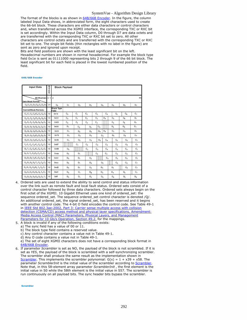
SystemVue - Algorithm Design Library
292
The format of the blocks is as shown in 64B/66B Encoder. In the figure, the columnlabeled Input Data shows, in abbreviated form, the eight characters used to createthe 66-bit block. These characters are either data characters or control charactersand, when transferred across the XGMII interface, the corresponding TXC or RXC bitis set accordingly. Within the Input Data column, D0 through D7 are data octets andare transferred with the corresponding TXC or RXC bit set to zero. All othercharacters are control octets and are transferred with the corresponding TXC or RXCbit set to one. The single bit fields (thin rectangles with no label in the figure) aresent as zero and ignored upon receipt.Bits and field positions are shown with the least significant bit on the left.Hexadecimal numbers are shown in normal hexadecimal. For example the block typefield 0x1e is sent as 01111000 representing bits 2 through 9 of the 66 bit block. Theleast significant bit for each field is placed in the lowest numbered position of thefield.
64B/66B Encoder
Ordered sets are used to extend the ability to send control and status information4.over the link such as remote fault and local fault status. Ordered sets consist of acontrol character followed by three data characters. Ordered sets always begin on thefirst octet of the XGMII. 10 Gigabit Ethernet uses one kind of ordered_set: thesequence ordered_set. The sequence ordered_set control character is denoted /Q/.An additional ordered_set, the signal ordered_set, has been reserved and it beginswith another control code. The 4-bit O field encodes the control code. See Table 49-1in IEEE Std 802.3ae-2002, Part 3: Carrier sense multiple access with collisiondetection (CSMA/CD) access method and physical layer specifications, Amendment:Media Access Control (MAC) Parameters, Physical Layers, and ManagementParameters for 10 Gb/s Operation, Section 49.2. for the mappings.A block is invalid if any of the following conditions exists:5.a) The sync field has a value of 00 or 11.b) The block type field contains a reserved value.c) Any control character contains a value not in Table 49-1.d) Any O code contains a value not in Table 49-1.e) The set of eight XGMII characters does not have a corresponding block format in64B/66B Encoder.If parameter Scrambler is set as NO, the payload of the block is not scrambled. If it is6.set as YES, the payload of the block is scrambled with a self-synchronizing scrambler.The scrambler shall produce the same result as the implementation shown inScrambler. This implements the scrambler polynomial: G(x) = 1 + x39 + x58. Theparameter ScramblerInit is the initial value of the scrambler according to Scrambler.Note that, in this 58-element array parameter ScramblerInit , the first element is theinitial value in S0 while the 58th element is the initial value in S57. The scrambler isrun continuously on all payload bits. The sync header bits bypass the scrambler.
Scrambler

SystemVue - Algorithm Design Library
293
Each firing,7.64 tokens are consumed at pin input, and 8 tokens are consumed at pin CtrlBits.66 tokens are produced at pin output.The input at pin input are 8 data octets or control characters. For each dataoctet or control character, the LSB is input first.Each token at pin CtrlBits indicates the type of corresponding octet at pin input.0 indicates data octet while 1 indicates control character.All the bits are input and output serially.
References
IEEE Std 802.3ae-2002, Part 3: Carrier sense multiple access with collision detection1.(CSMA/CD) access method and physical layer specifications, Amendment: MediaAccess Control (MAC) Parameters, Physical Layers, and Management Parameters for10 Gb/s Operation, Section 49.2.

SystemVue - Algorithm Design Library
294
Decoder8b10b PartCategories: C++ Code Generation (algorithm), IBIS-AMI Transceivers (algorithm)
The models associated with this part are listed below. To view detailed information on amodel (description, parameters, equations, notes, etc.), please click the appropriate link.
Model Description
Decoder8b10b(algorithm)
8b/10b decoder

SystemVue - Algorithm Design Library
295
Decoder8b10b
Description: 8b/10b decoderDomain: UntimedC++ Code Generation Support: YESAssociated Parts: Decoder8b10b Part (algorithm)
Model Parameters
Name Description Default Units Type Runtime Tunable
Delay number of 10-bit symboldelay
0 Integer NO
Input Ports
Port Name Signal Type Optional
1 input int NO
Output Ports
Port Name Signal Type Optional
2 output int NO
3 Kout int NO
Notes/Equations
The 8B/10B decoder is the reverse procedure of 8B/10B encoder. It's illustrated in1.Decoder 8B/10B.
Decoder 8B/10B
For more information on the 8B/10B Coder, refer to Coder8b10b (algorithm).Parameter Description:2.Delay specifies the number of 10-bit symbol delay. The decoder begins to work after10*Delay input tokens.Each firing,3.
Ten tokens are consumed at pin input. One token is produced at pin Kout(control character), and eight tokens are produced at pin output.All the bits are input and output serially.The input at pin input is the 10-bit transmission code-group. The LSB bit (a) isinput first, while the MSB (j) is input last.The output at pin Kout is the decoded control variable Z, in which 0 means thevalue D and 1 means the value K.The output at pin output is the decoded information octet. The LSB bit (A) isoutput first, while the MSB (H) is output last.
References
IEEE Std 802.3, 2000 Edition, Part 3: Carrier sense multiple access with collision1.detection (CSMA/CD) access method and physical layer specifications, Section36.2.4.

SystemVue - Algorithm Design Library
296
Decoder64b66b PartCategories: C++ Code Generation (algorithm), IBIS-AMI Transceivers (algorithm)
The models associated with this part are listed below. To view detailed information on amodel (description, parameters, equations, notes, etc.), please click the appropriate link.
Model Description
Decoder64b66b(algorithm)
64b/66bdecoder

SystemVue - Algorithm Design Library
297
Decoder64b66b
Description: 64b/66b decoderDomain: UntimedC++ Code Generation Support: YESAssociated Parts: Decoder64b66b Part (algorithm)
Model Parameters
Name Description Default Units Type RuntimeTunable
Scrambler scramble ornot: NO,YES
NO Enumeration NO
ScramblerInit initial stateof scrambler
[1,1,1,1,1,1,1,1,1,1,1,1,1,1,1,1,1,1,1,1,1,1,1,1,1,1,1,1,1,1,1,1,1,1,1,1,1,1,1,1,1,1,1,1,1,1,1,1,1,1,1,1,1,1,1,1,1,1] Integerarray
NO
Delay number of66-bitsymboldelayed fordescrambler
0 Integer NO
Input Ports
Port Name Signal Type Optional
1 input int NO
Output Ports
Port Name Signal Type Optional
2 output int NO
3 CtrlBits int NO
Notes/Equations
The 64B/66B decoder is the reverse procedure of the 64B/66B encoder. For more1.information on the 64B/66B Coder, refer to Coder64b66b (algorithm).Parameter Description:2.If parameter Scrambler is set as NO, the payload of the block is not scrambled. If it isset as YES, the payload of the block is scrambled with a self-synchronizing scrambler.The scrambler shall produce the same result as the implementation shown inScrambler. This implements the scrambler polynomial: G(x) = 1 + x39 + x58. Theparameter ScramblerInit is the initial value of the scrambler according to Scrambler.Note that, in this 58-element array parameter ScramblerInit, the first element is theinitial value in S0 while the 58th element is the initial value in S57. The scrambler isrun continuously on all payload bits. The sync header bits bypass the scrambler.
Scrambler
Parameter Delay specifies the number of 66-bit symbol delay. The decoder begins towork after 66* Delay input tokens.Each firing,3.
66 tokens are consumed at pin input. 64 tokens are produced at pin output, and8 tokens are produced at pin CtrlBits (with each corresponding to 8 decodedbits).The output at pin output are 8 data octets or control characters. For each dataoctet or control character, the LSB is input first.Each token at pin CtrlBits indicates the type of corresponding output octet at pinoutput. 0 indicates data octet while 1 indicates control character.All the bits are input and output serially.

SystemVue - Algorithm Design Library
298
References
IEEE Std 802.3ae-2002, Part 3: Carrier sense multiple access with collision detection1.(CSMA/CD) access method and physical layer specifications, Amendment: MediaAccess Control (MAC) Parameters, Physical Layers, and Management Parameters for10 Gb/s Operation, Section 49.2.

SystemVue - Algorithm Design Library
299
DFE PartCategories: C++ Code Generation (algorithm), IBIS-AMI Transceivers (algorithm)
The models associated with this part are listed below. To view detailed information on amodel (description, parameters, equations, notes, etc.), please click the appropriate link.
Model Description
DFE (algorithm) Decision-Feedback Equalizer
BlindDFE(algorithm)
Blind Decision Feedback Equalizer

SystemVue - Algorithm Design Library
300
DFE
Description: Decision-Feedback EqualizerDomain: UntimedC++ Code Generation Support: YESAssociated Parts: DFE Part (algorithm), BlindDFE Part (algorithm)
Model Parameters
Name Description Default Units Type RuntimeTunable
ChannelImpulse Channel impulse response vectorrepresenting the overall impulse responsefrom bit source to the input of FFE
[1] None NO
SamplesPerBit 16 Integer NO
NumDFETaps Number of DFE taps 0 Integer NO
SampleInterval Sample interval associated with thechannel impulse response
1e-10 s Float NO
LogicLevel Logic level of the binary bits injected intothe channel. Bit 1 and 0 are representedby LogicLevel and -LogicLevel.
1.0 V Float NO
BitSampling Bit sampling point: Negative clock edge,Positive clock edge
Positiveclock edge
Enumeration NO
AdaptiveEQ Adaptive equalization option: NO, YES YES Enumeration NO
Alpha Taps update factor 0.01 Float NO
StartThreshold Magnitude threshold of the input signal tostart the adaptive process
0 Float NO
LimitCoefficients Enable adaptation range limits for thecoefficients: NO, YES
NO Enumeration NO
CoefficientMaximums Maximum limits for bit level DFE taps None NO
CoefficientMinimums Minimum limits for bit level DFE taps None NO
PrecedingEqualizer Equalizer preceded before DFE: None,FFE
None Enumeration NO
FFENumPrecursorTaps Number of FFE precursor taps. Total FFEtaps = NumPrecursorTaps +NumPostcursorTaps + 1.
0 Integer NO
FFENumPostcursorTaps Number of FFE postcursor taps. Total FFEtaps = NumPrecursorTaps +NumPostcursorTaps + 1.
0 Integer NO
FFENormalization Normalize FFE coefficients to have unitsum: NO, YES
NO Enumeration NO
Input Ports
Port Name Signal Type Optional
1 input real NO
2 clock int NO
Output Ports
Port Name Signal Type Optional
3 output real NO
4 bit int NO
Notes/Equations
DFE implements adaptive decision feedback equalizer and automatically computes1.optimal bit-level DFE taps based on the given channel impulse response (parameterChannelImpulse) using LMS algorithm.This model consumes one sample from the input port and one sample from the2.clock port and produces one sample to the output port and one sample to the bitport in every execution.Parameter PrecedingEqualizer specifies the equalizer precedes DFE. If3.PrecedingEqualizer is set to None, parameter ChannelImpulse specifies theoverall impulse response of the system starting right after the bit source andstopping right before the DFE. If PrecedingEqualizer is set to FFE, parameterChannelImpulse specifies the overall impulse response of the system starting rightafter the bit source and stopping right before the FFE (algorithm). When computingoptimal DFE taps, the effect of FFE (algorithm) will be taken into account.Parameter NumDFETaps specifies the number of desired DFE taps.4.Please refer to FFE (algorithm) for parameters ChannelImpulse, SamplesPerBit,5.

SystemVue - Algorithm Design Library
301
SampleInterval, and LogicLevel.Please refer to BlindDFE (algorithm) for parameters BitSampling, AdaptiveEQ,6.Alpha, and StartThreshold.If PrecedingEqualizer is set to FFE, please refer to FFE (algorithm) for parameters7.FFENumPrecursorTaps, FFENumPostcursorTaps, and FFENormalization.Please refer to BlindDFE (algorithm) for DFE operation.8.Use BlindDFE (algorithm) instead of DFE (algorithm) if you want to specify a set of9.custom taps.

SystemVue - Algorithm Design Library
302
FFE PartCategories: C++ Code Generation (algorithm), IBIS-AMI Transceivers (algorithm)
The models associated with this part are listed below. To view detailed information on amodel (description, parameters, equations, notes, etc.), please click the appropriate link.
Model Description
FFE (algorithm) Feed-Forward Equalizer
BlindFFE(algorithm)
Blind Feed-ForwardEqualizer

SystemVue - Algorithm Design Library
303
FFE
Description: Feed-Forward EqualizerDomain: UntimedC++ Code Generation Support: YESAssociated Parts: FFE Part (algorithm), BlindFFE Part (algorithm)
Model Parameters
Name Description Default Units Type RuntimeTunable
ChannelImpulse Channel impulse response vector representingthe overall impulse response from bit source tothe input of FFE
[1] None NO
SamplesPerBit Number of samples per bit 16 Integer NO
NumPrecursorTaps Number of precursor taps. Total FFE taps =NumPrecursorTaps + NumPostcursorTaps + 1.
0 Integer NO
NumPostcursorTaps Number of postcursor taps. Total FFE taps =NumPrecursorTaps + NumPostcursorTaps + 1.
0 Integer NO
SampleInterval Sample interval associated with the channelimpulse response
1e-10 s Float NO
LogicLevel Logic level of the binary bits injected into thechannel. Bit 1 and 0 are represented byLogicLevel and -LogicLevel.
1.0 V Float NO
Normalization Normalize FFE coefficients to have unit sum:NO, YES
NO Enumeration NO
Input Ports
Port Name Signal Type Optional
1 input real NO
Output Ports
Port Name Signal Type Optional
2 output real NO
Notes/Equations
FFE implements feed-forward equalizer and automatically computes optimal bit-level1.FFE taps based on the given channel impulse response (parameter ChannelImpulse) using LMS algorithm.This model consumes one sample from the input port and produces one sample tothe output port.Parameter ChannelImpulse specifies the overall impulse response of the system2.starting right after the bit source and stopping right before the FFE, which canpossibly include transmitter, channel, and receiver frond-end, etc.
Let denote such impulse response specified byChannelImpulse, where L is the length of the given channel impulse response.
Parameter SamplesPerBit specifies the number of samples per bit used in the3.simulation, which is equivalent to bit time (unit interval (UI)) divided by sampleinterval.Parameter NumPrecursorTaps and NumPostcursorTaps specify the number of4.precursor taps N1 and the number of postcursor taps N2 to be used in FFE. The totalnumber of FFE taps including the main cursor is N1+N2+1.Parameter LogicLevel specifies logic one voltage, LogicLevel, and logic zero voltage, -5.LogicLevel, in the NRZ (non-return-to-zero) format. The bit stream injected into thechannel is assumed in the NRZ format.
Let b[n] = 1 or 0 represent random bits.Let N denote number of samples per bit.Set V = LogicLevel.The sampled version of bits b[k] in the NRZ format can be expressed in z[n] as:
Parameter SampleInterval specifies sampling interval used in the simulation.6.Sample interval is equivalent to 1 / sampling rate.The FFE input signal x[n] is assumed to be the output of channel h when the input to7.the channel is z[n]. Assuming channel h is a LTI (linear time-invariant) system, thenx[n] can be expressed as
The convolution in this context involves a scaling factor of sample interval. Thisconvention is commonly adopted by many channel simulators.ChannelImpulse h[n] should be scaled properly to take sample interval into

SystemVue - Algorithm Design Library
304
account.Based on the given channel impulse and other parameters, FFE automatically8.computes a set of bit-level taps to remove ISI (inter symbolinterference). The number of FFE taps M is N1_N2_1.When parameter Normalization is set to NO, the amplitude of output samples is9.approximately in the range of 1 and -1. When parameter Normalization is set toYES, then w[n] is normalized to have unit sum, i.e., Let y[n] denote the output samples of FFE. The FFE operation can be expressed as:10.
See also BlindFFE (algorithm). Use BlindFFE (algorithm) instead of FFE if you want to11.specify a set of custom taps.

SystemVue - Algorithm Design Library
305
JitterGenerator PartCategories: C++ Code Generation (algorithm), IBIS-AMI Transceivers (algorithm)
The models associated with this part are listed below. To view detailed information on amodel (description, parameters, equations, notes, etc.), please click the appropriate link.
Model Description
JitterGenerator(algorithm)
Jitter generator
JitterGenerator
Description: Jitter generatorDomain: TimedC++ Code Generation Support: YESAssociated Parts: JitterGenerator Part (algorithm)
Model Parameters
Name Description Default Units Type RuntimeTunable
VHigh the Logic-1 voltage level 1 V Float NO
VLow the Logic-0 voltage level -1 V Float NO
EdgeTime the rise and fall times (in second) : must be in therange between 0.0 and 0.5 UI
0.0 s Float NO
SamplesPerUI the number of samples per UI 16 Integer NO
InitialState the initial state for the sequence 0 Integer NO
DCD Duty-cycle distortion (in second): must be in the rangebetween 0.0 and 1.0 UI
0 s Float YES
PJ_Amplitude Periodic jitter amplitude in sec 0 s Float YES
PJ_Frequency Periodic jitter frequency in Hz 0 Hz Float YES
RJ RMS random jitter (in second):must be in the rangebetween 0.0 and 1.0 UI
0 s Float YES
Input Ports
Port Name Description Signal Type Optional
1 Input the input sequences int NO
Output Ports
Port Name Description Signal Type Optional
2 Output the output sampledbits
real NO
Notes/Equations
This model is used to apply random, periodic and DCD jitter to the input bit.1.Upsampling with rise/fall edge is also applied.Each firing,2.
1 token is consumed at the input port.SamplesPerUI tokens are produced at the output port. It equals to 16 bydefault.
Parameter details:3.VHigh specifies the logic-1 voltage level of the input sequences.VLow specifies the logic-0 voltage level of the input sequences.EdgeTime specifies the rise/fall times in second.SamplesPerUI specifies the number of samples for one input bit.InitialState specifies the initial state of the input sequence.DCD specifies the Duty-cycle distortion in second.PJ_Amplitude specifies the periodic Jitter amplitude in second.PJ_Frequency specifies the periodic Jitter frequency in Hz.RJ specifies the random Jitter in second.
The input sequences should be logical bit which can only be 1 or 0. This is a timed4.model so that bit rate can be got from the input port. Timing Jitter is defined as thedeviation of a signal transition from its ideal position in time. The total Jitter consistsof two components: the Deterministic Jitter(DJ) and Random Jitter(RJ).
DCD is a part of Deterministic Jitter which is caused by a difference inpropagation delay between low to high transitions and high to low transitions.Assuming the ideal signal has 50% duty cycle, the deviated signal with DCD hasnon-50% duty cycle.
SystemVue - Algorithm Design Library
306
Periodic Jitter is a part of Deterministic Jitter which is caused by electromagneticinterference. This type of deviation is referred to as Sinusoidal which repeats in
a cyclic fashion. The model is represented as:
where denotes the total periodic jitter, N is the number of cosinecomponents(tones), Ai is the amplitude in units of time, is the modulationfrequency, t is the time and is the initial phase. This model is applied as:
.Random Jitter which comes from device noise sources such as thermal andflicker noise is characterized by both Gaussian and non-Gaussian distributions.This model only support Gaussian distribution with mean value equals to 0 andstandard deviation equals to 1.
This model causes one bit time delay.5.
References
Kyung Ki Kim, Jing Huang, Yong-Bin Kim, Fabrizio Lombard. "On the Modeling and1.Analysis of Jitter in ATE Using Matlab". Proceedings of the 20th IEEE InternationalSymposium on Defect and Fault Tolerance in VLSI Systems, pp. 285-293,2005.

SystemVue - Algorithm Design Library
307
PhaseDetector PartCategories: C++ Code Generation (algorithm), IBIS-AMI Transceivers (algorithm)
The models associated with this part are listed below. To view detailed information on amodel (description, parameters, equations, notes, etc.), please click the appropriate link.
Model Description
PhaseDetector(algorithm)
PhaseDetector
PhaseDetector
Description: PhaseDetectorDomain: UntimedC++ Code Generation Support: YESAssociated Parts: PhaseDetector Part (algorithm)
Model Parameters
Name Description Default Units Type RuntimeTunable
BitCenter Bit center and clock edge alignment: Negativeclock edge, Positive clock edge
Positive clockedge
Enumeration NO
Input Ports
Port Name Signal Type Optional
1 signal real NO
2 clock int NO
Output Ports
Port Name Signal Type Optional
3 phaseError real NO
Notes/Equations
PhaseDetector detects phase difference (phase error) between input signal and1.reference clock.The phase detection method used in this model is derived from: C. R. Hogge Jr. "A2.self correcting clock recovery circuit", IEEE Transactions on Electron Devices, 1985.This model consumes one sample from signal and one sample from clock and3.produces one sample to phaseError in every execution.PhaseDetector assumes signal is in NRZ (non-return-to-zero) format. If a signal4.sample is larger than 0, it is treated as bit level 1, otherwise, it is treated as bit level0.PhaseDetector treats positive-valued clock sample as clock level 1 and treats non-5.positive-valued clock sample as clock level 0.The PhaseDetector detects phase difference (phase error) between the bit transition6.of the input signal and the clock edge.Suppose BitCenter is set to Negative clock edge, signal and clock are synchronized7.(no phase error) if the negative clock edge is aligned with the bit center. On theother hand, suppose BitCenter is set to Positive clock edge, there is no phase error ifthe positive clock edge is aligned with the bit center.PhaseDetector can only detect phase error when there is a bit transition in the input8.signal. When there is a bit transition, the phase error is outputted at the next positiveclock edge if BitCenter is set to Negative clock edge. Otherwise (BitCenter is set toPositive clock edge), the phase error is outputted at the next negative clock edge. Forall other situations, phaseError outputs 0.Phase error is computed in rad. However, due to discrete-time implementation, the9.number of possible phase error values are equivalent to the number of samples perbit (samples per unit interval), which are equally spaced in the range of

SystemVue - Algorithm Design Library
308
PulseShaping PartCategories: C++ Code Generation (algorithm), IBIS-AMI Transceivers (algorithm)
The models associated with this part are listed below. To view detailed information on amodel (description, parameters, equations, notes, etc.), please click the appropriate link.
Model Description
PulseShaping(algorithm)
Jitter generator

SystemVue - Algorithm Design Library
309
PulseShaping
Description: Jitter generatorDomain: TimedC++ Code Generation Support: YESAssociated Parts: PulseShaping Part (algorithm)
Model Parameters
Name Description Default Units Type RuntimeTunable
VHigh the Logic-1 voltage level 1 V Float NO
VLow the Logic-0 voltage level -1 V Float NO
EdgeTime the rise and fall times (in second) : must be in therange between 0.0 and 0.5 UI
0.0 s Float NO
SamplesPerUI the number of samples per UI 16 Integer NO
InitialState the initial state for the sequence 0 Integer NO
DCD Duty-cycle distortion (in second): must be in the rangebetween 0.0 and 1.0 UI
0 s Float YES
PJ_Amplitude Periodic jitter amplitude in sec 0 s Float YES
PJ_Frequency Periodic jitter frequency in Hz 0 Hz Float YES
RJ RMS random jitter (in second):must be in the rangebetween 0.0 and 1.0 UI
0 s Float YES
Input Ports
Port Name Description Signal Type Optional
1 Input the input sequences int NO
Output Ports
Port Name Description Signal Type Optional
2 Output the output sampledbits
real NO
Notes/Equations

SystemVue - Algorithm Design Library
310
TimeResponseFIR Part
Categories: C++ Code Generation (algorithm), IBIS-AMI Transceivers (algorithm)
The models associated with this part are listed below. To view detailed information on amodel (description, parameters, equations, notes, etc.), please click the appropriate link.
Model
TimeResponseFIR(algorithm)

SystemVue - Algorithm Design Library
311
TimeResponseFIR
Description:Domain: UntimedC++ Code Generation Support: YESAssociated Parts: TimeResponseFIR Part (algorithm)
Model Parameters
Name Description Default Units Type RuntimeTunable
ResponseType Type of Response specified:Impulse Response, Step Response
StepResponse
Enumeration NO
Response Time Response Coefficients Floating pointarray
NO
ResponseTimeStamps Time Stamps of time responsecoefficients, must be in ascendingorder
Floating pointarray
NO
SampleRate Input signal sampling rate 10.3125e9*16 Hz Float NO
Input Ports
Port Name Signal Type Optional
1 input real NO
Output Ports
Port Name Signal Type Optional
2 output real NO
Notes/Equations
TimeResponseFIR can be used to recharacterize step or impulse response specified withResponse and ResponseTimeStamps at a user specified TimeStep. The user specefiedResponse is usually measured either in the lab using measurement equipments or usingcircuit simulators such as H-Spice. If the ResponseType is Impulse Response then a 4-point Lagrange interpolation is performed to calculate recharacterized impulse responsewith specified Time Step. If the ResponseType is Step Response then analyticaldifferentiation is performed on input response in the time vicinity of each coefficient ofrecharacterized impulse response to calculate the value of the coefficient at the accuratetime specified using Time Step. The recharacterized impulse response coefficients are thenused as FIR taps. In case of ResponseType being Step Response, output of the FIR isalso multiplied with TimeStep value.
The number of coefficients in the recharacterized impulse response are calculated as (max ( ResponseTimeStamps ) - min ( ResponseTimeStamps ) ) / TimeStep.
The values in ResponseTimeStamps must be positive and in non-repeating ascendingorder.

SystemVue - Algorithm Design Library
312
VCO PartCategories: C++ Code Generation (algorithm), IBIS-AMI Transceivers (algorithm)
The models associated with this part are listed below. To view detailed information on amodel (description, parameters, equations, notes, etc.), please click the appropriate link.
Model Description
VCO(algorithm)
Voltage ControlledOscillator
VCO
Description: Voltage Controlled OscillatorDomain: UntimedC++ Code Generation Support: YESAssociated Parts: VCO Part (algorithm)
Model Parameters
Name Description Default Units Type Runtime Tunable
SampleInterval Sample interval in sec. 1e-10 s Float NO
Frequency Fundamental oscillator frequency in Hz. 1e9 Hz Float NO
Sensitivity Sensitivity in Hz/V. 1 Float NO
InitialPhase Initial phase in rad. 0 deg Float NO
Amplitude Output amplitude in volt. 1 V Float NO
Input Ports
Port Name Signal Type Optional
1 vin real NO
Output Ports
Port Name Signal Type Optional
2 vout real NO
3 clock int NO
Notes/Equations
VCO implements voltage-controlled oscillator.1.This model consumes one sample from vin and produces one sample to vout and to2.clock in every execution.The continuous-time input-output relationship of voltage-controlled oscillator can be3.expressed as , where represents input voltagevin, represents output voltage vout, represents oscillator fundamentalFrequency in Hz, represents Sensitivity in Hz/volt, represents InitialPhase inrad, and represents Amplitude in volt.VCO is implemented as discrete-time version of the above equation. The sampling4.time instances are at , where and represents sampling TimeStep.The clock port outputs square clock waveform samples. The clock samples are5.
generated by slicing using the following equation:

SystemVue - Algorithm Design Library
313
WriteFlexDCAFile PartCategories: C++ Code Generation (algorithm), IBIS-AMI Transceivers (algorithm)
The models associated with this part are listed below. To view detailed information on amodel (description, parameters, equations, notes, etc.), please click the appropriate link.
Model Description
WriteFlexDCAFile(algorithm)
Write samples in a text file that conforms to the Agilent FlexDCA Softwarerequirements
WriteFlexDCAFile
Description: Write samples in a text file that conforms to the Agilent FlexDCA SoftwarerequirementsDomain: TimedC++ Code Generation Support: YESAssociated Parts: WriteFlexDCAFile Part (algorithm)
Model Parameters
Name Description Default Units Type RuntimeTunable
FileName Wave samples text file MyPatternWave.txt Filename NO
NumToSkip Number of bits to skip before writingto text file.
0 Integer NO
NumToCollect Number of bits to be collected andwritten into the text file.
1 Integer NO
PeriodicPattern Bits pattern is periodic (Required forjitter analysis): NO, YES
YES Enumeration NO
BitRate Original bit rate. Sample_Rate Hz Float NO
PatternLength Number of bits per period for periodicbit pattern.
1 Integer NO
Input Ports
Port Name Signal Type Optional
1 m_cbInput real NO
Notes/Equations

SystemVue - Algorithm Design Library
314
WriteN1000AFile PartCategories: C++ Code Generation (algorithm), IBIS-AMI Transceivers (algorithm)
The models associated with this part are listed below. To view detailed information on amodel (description, parameters, equations, notes, etc.), please click the appropriate link.
Model Description
WriteN1000AFile(algorithm)
Write samples in a text file that conforms to the Agilent N1000A Softwarerequirements

SystemVue - Algorithm Design Library
315
WriteN1000AFile
Description: Write samples in a text file that conforms to the Agilent N1000A SoftwarerequirementsDomain: TimedC++ Code Generation Support: YESAssociated Parts: WriteN1000AFile Part (algorithm)
Model Parameters
Name Description Default Units Type RuntimeTunable
FileName Wave samples text file MyPatternWave.txt Filename NO
NumToSkip Number of bits to skip before writingto text file.
0 Integer NO
NumToCollect Number of bits to be collected andwritten into the text file.
1 Integer NO
PeriodicPattern Bits pattern is periodic (Required forjitter analysis): NO, YES
YES Enumeration NO
BitRate Original bit rate. Sample_Rate Hz Float NO
PatternLength Number of bits per period for periodicbit pattern.
1 Integer NO
Input Ports
Port Name Signal Type Optional
1 m_cbInput real NO
Notes/Equations

SystemVue - Algorithm Design Library
316
SignalDownloader_81180 Part 81180 AWG Downloader
Categories: Instrumentation (algorithm)
The models associated with this part are listed below. To view detailed information on amodel (description, parameters, equations, notes, etc.), please click the appropriate link.
Model
SignalDownloader_81180(algorithm)
SignalDownloader_81180
Description: 81180 AWG DownloaderAssociated Parts: SignalDownloader 81180 Part (algorithm)
Model Parameters
Name Description Default Units Type RuntimeTunable
HWAvailable YES: HW available. NO: HW notexist: NO, YES
NO Enumeration NO
IOType Instrument Communication type:'LAN', 'TCPIP', or 'GPIB'
LAN Text NO
PrimAddress Primary address: IP address(LAN) or instrument GPIBaddress (GPIB)
111.222.333.444 Text NO
SecAddress Secondary address: Port number(LAN) or secondary address(GPIB)
5025 Integer NO
TimeStart Time to start waveform recording Start_Time Float NO
TimeStop Time to stop waveform recording Stop_Time Float NO
FileName File name for the downloadedwaveform
wave81180A.bin Text NO
OutputAmplifier Select Output Amplifier: DC, AC,DAC
DC none Enumeration NO
AmplitudeOutputDC amplitude in V (range: 0.05V -2V)
0.5 V Float NO
AmplitudeOutputAC_dBm amplitude in dBm (range. -5dBmto +5dBm)
0 Float NO
AmplitudeOutputDAC amplitude in V (range: 50mV -500mV)
500 mV Float NO
ShowAdvancedParams To display parameters foradvanced instrument setups: NO,YES
NO Enumeration NO
SCPICommands Additonal SCPI commands beforeturning ARB and RF output ON orOFF
Text NO
AutoScale Normalize waveform into [-1, 1]Volt range before downloading.YES: auto scale; NO: no autoscale.: NO, YES
YES Enumeration NO
InstructionTimeout Instrument instruction timeoutlimit
10 ms Float NO
ConfigMIMO Establish the Master-Slaverelationship among multiple81180; 1:YES, 0:NO: NO, YES
NO Enumeration NO
MasterSrc Mark this 81180 as the masterthat will generate thesynchronization trigger ; 1:YES,0:NO: NO, YES
NO Enumeration NO
Input Ports
Port Name Signal Type Optional
1 EnvelopIn complex NO

SystemVue - Algorithm Design Library
317
SignalDownloader_E4438C Part Signal Downloader for Agilent ESG E4438C and MXG N5182A RF Signal Synthesizers.
Categories: Instrumentation (algorithm)
The models associated with this part are listed below. To view detailed information on amodel (description, parameters, equations, notes, etc.), please click the appropriate link.
Model
SignalDownloader_E4438C(algorithm)
SignalDownloader_E4438C
Description: SignalDownloaderCategory: InstrumentationDomain:Associated Part: SignalDownloader E4438C Part (algorithm)
Basic Parameters
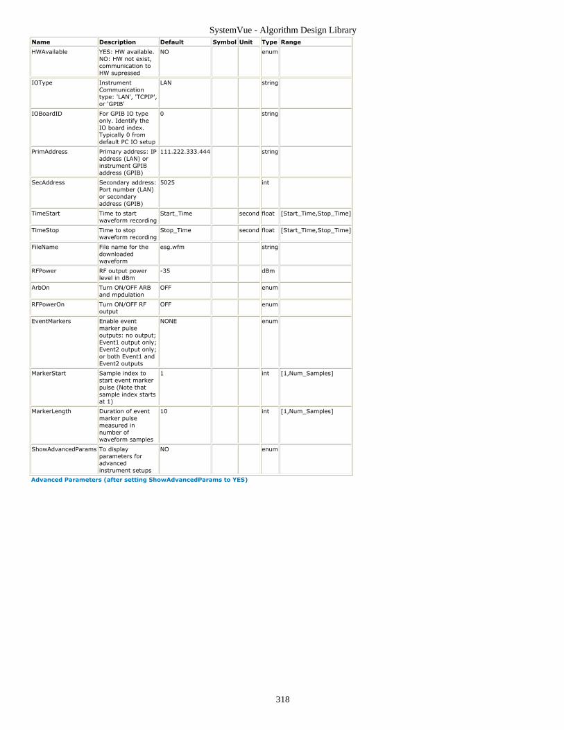
SystemVue - Algorithm Design Library
318
Name Description Default Symbol Unit Type Range
HWAvailable YES: HW available.NO: HW not exist,communication toHW supressed
NO enum
IOType InstrumentCommunicationtype: 'LAN', 'TCPIP',or 'GPIB'
LAN string
IOBoardID For GPIB IO typeonly. Identify theIO board index.Typically 0 fromdefault PC IO setup
0 string
PrimAddress Primary address: IPaddress (LAN) orinstrument GPIBaddress (GPIB)
111.222.333.444 string
SecAddress Secondary address:Port number (LAN)or secondaryaddress (GPIB)
5025 int
TimeStart Time to startwaveform recording
Start_Time second float [Start_Time,Stop_Time]
TimeStop Time to stopwaveform recording
Stop_Time second float [Start_Time,Stop_Time]
FileName File name for thedownloadedwaveform
esg.wfm string
RFPower RF output powerlevel in dBm
-35 dBm
ArbOn Turn ON/OFF ARBand mpdulation
OFF enum
RFPowerOn Turn ON/OFF RFoutput
OFF enum
EventMarkers Enable eventmarker pulseoutputs: no output;Event1 output only;Event2 output only;or both Event1 andEvent2 outputs
NONE enum
MarkerStart Sample index tostart event markerpulse (Note thatsample index startsat 1)
1 int [1,Num_Samples]
MarkerLength Duration of eventmarker pulsemeasured innumber ofwaveform samples
10 int [1,Num_Samples]
ShowAdvancedParams To displayparameters foradvancedinstrument setups
NO enum
Advanced Parameters (after setting ShowAdvancedParams to YES)

SystemVue - Algorithm Design Library
319
Name Description Default Symbol Unit Type Range
Reset Reset the instrument before everything else.YES: reset instrument; NO: skip instrumentreset
YES enum
IQModFilter Filter applied to played out IQ (ARB) waves:THROUGH (no filter applied); 2.1MHz Low LassFilter; 40MHz Low pass Filter
THROUGH enum
SCPICommands Additonal SCPI commands before turning ARBand RF output ON or OFF
string
AutoScale Normalize waveform into [-1, 1] Volt rangebefore downloading. YES: auto scale; NO: noauto scale
YES enum
InstructionTimeout Instrument instruction timeout limit 10 second float
ARBRefSrc Source for ARB reference frequency, either:provided internally by the instrument(INTERNAL) or provided by an externalinstrument (EXTERNAL)
INTERNAL enum
ARBRefFreq ARB reference frequency (Active only whenchosen EXTERNAL ARB reference)
10e6 Hz float
ConfigMIMO Establish the Master-Slaves relationship amongmultiple E4438C or MXG(N5182A) signalgenerators. YES: Instrument participates MIMOsetup; NO: Instrument doesn't participateMIMO setup
NO enum
MasterSrc Mark this signal source as the master that willgenerate the synchronization trigger fromEVENT1 (MXG) or EVENT2 (E4438C). YES:Master source; NO: Slave source
NO enum
UseE4438Cs YES = E4438C's are used; NO = MXG's areused
YES enum
NumMXGSlaves (For MXG's only) Number of MXG Slaves(range: 1 to 15)
1 int [1, 15]
SlavePosition (For slave MXG's only) Slave position (Range: 1to 15)
1 int [1, 15]
Input Ports
Port Name Description Signal Type Optional
1 input input signal Complex Envelope (i.e. Modulated RF signal) NO
Example: ESG SignalDownloader Example.wsv under Instruments Examples(examples)
SignalDownloader_E4438C supports both Agilent ESG E4438C, MXG N5182A, and PSG E8267Dseries instruments
SignalDownloader_E4438C only accepts Timed Complex Envelope (also known as Timedmodulated RF) signal. Make sure you use a part such as RF Modulator (algorithm) part in front of it toconvert complex IQ signal into Complex Envelope signal. If the complex IQ signal does not havesampling time information, make sure to use a SetSampleRate (algorithm) part in front of the RFModulator (algorithm) part to set up the sampling rate for the baseband IQ waveform.
How to determine if a signal is "Timed"? Open the Source part (e.g. SineGen, Bits, etc)used in thedesign/schematic, set "ShowAdvancedParams = YES"; the "SampleRateOption" should be"1:Timed from SampleRate" ( recommended default setting) or "2:Timed from Schematic" fortimed signals.
In current SystemVue release, "LAN" is the only IOType supported.
Where do the values for variables such as Num_Samples, Start_Time or Stop_Time come from? Theyall come from the simulation controller for Data Flow simulation.Create a workspace from the Blank template. Then double click the "Design1 Analysis" on the workspacetree, it will bring up the "Data Flow Analysis (sim)" window, the simulation controller.The "Start_Time" contains the value in the Start Time: field, the "Stop_Time" for the Stop Time:, andof course, the "Num_Samples" for Number of Samples.
Master-Slave(s) Configuration for MIMO Applications
Using E4438C's - Example: ESG MIMO Configuration Example.wsv under InstrumentsExamples (examples)
1.
Configure the interconnections between the master and slave E4438C's asshown in the diagram. (Note: You can add more slave E4438C's in the sameway as the existing slave).The 10 MHz references should be connected between the instruments.The EVENT2 output of the master E4438C is used to generate thesynchronization trigger and can't be used to as EventMarker outputs.Master or slave status is controlled by the MasterSrc parameter.Make sure to set ARBRefSrc = EXTERNAL

SystemVue - Algorithm Design Library
320
Using N5182A's - Example: MXG MIMO Configuration Example.wsv under InstrumentsExamples (examples)
1.
Make sure that the EVENT 1 output from the master MXG (N5182A) isconnected to the PAT TRIG IN on the slave MXG.If additional slaves are present, the EVENT 1 output of each slave should beconnected to the PAT TRIG IN of the next slave in the system.The 10 MHz references should be connected between the instruments.
Make sure to leave ARBRefSrc at its default INTERNAL state. MXG's will automaticallysense the reference signals and adjust itself accordingly.
Make sure ArbOn is set to "OFF". You have to use MathLang script (users) to run thesimulation followed by turning ON the baseband ARB.
Make sure UseE4438Cs = "NO", and set up NumMXGSlaves for master MXGand set up NumMXGSlaves and SlavePosition for slave MXG('s) accordingly.
Notes/Equations
In addition to the E4438C (ESG-C Series) source instrument mentioned above,1.SignalDownloader_E4438C also supports the E8267C (PSG-C), E8267D (PSG-D),and N5182A (MXG). It provides an interface for streaming baseband IQ waveformsmodulated onto an RF carrier into the Agilent E4438C, N5182A, and E8267DVector Signal Synthesizers to produce the desired modulated RF signals at thespecified power level.SignalDownloader_E4438C only accepts Timed Complex Envelope (also known2.as Timed modulated RF) signal. Make sure you use a part such as RF Modulator(algorithm) part in front of it to convert complex IQ signal into Complex Envelopesignal. If the complex IQ signal does not have sampling time information, make sureto use a SetSampleRate (algorithm) part in front of the RF Modulator(algorithm) part to set up the sampling rate for the baseband IQ waveform.The EventMarkers parameter controls whether a pulse will be sent out at the3.instrument's Event1 and Event2 output. The pulses coming out of the two outputshave the same characteristics. The pulse rises at the sample indexed by theMarkerStart parameter and last the number of samples determined by theMarkerLength parameter.For example, assume the waveform contains 600 samples (i.e. 600 IQ pairs), if youwant a pulse to start at the 1st sample and last 10 sampling period, you simply setthe MarkerStart = 1 and MarkerLength = 10.The SCPICommands parameter holds additional instrument control SCPI commands4.you want to send to the instrument. The SCPI commands entered here will beexecuted right before the RF modulation and RF power are turned on. This means ifyou want to set RF powers or event markers again here, it will override the settingspassed in through the RFPower or EventMarkers parameters.The AutoScale parameter will force a normalization of the waveform generate to5.within [-1, 1]V range. The scaling is linear and the maximum magnitude of the I andQ data is scaled to -1V or 1V.If an instruction can not be completed within the time specified in the6.InstructionTimeout parameter, either due to IO communication issues or due to

SystemVue - Algorithm Design Library
321
hardware failures, a timeout will occur so that the simulator will not appear to hang.When you choose to hook your instrument with an external reference source, you7.need to set ARBRefFreq = EXTERNAL and specify the reference frequency providedby the external reference source here.
Important Links To learn more about the instruments supported by the SignalDownloader_E4438C,please visit the E4438C and MXG websites of Agilent Technologies.
Theory of Operation
SignalDownloader_E4438C is a sub-circuit part that is built upon the Sink (algorithm)part. It utilizes the Sink (algorithm) part's capability of executing a MathLangEquation (users) when all simulation data have been collected. Here is how theoperation flow goes. (To follow the following description, you can drop aSignalDownloader_E4438C part into the design/schematic and do a mouse right clickon the part to bring out the drop-down menuand select "Open -> Model/Subcircuit". You should see the sub-circuitdesign/schematic that has only a Sink (algorithm) in it. (An node namedSignalDownloader_ESG4438C(Model) will also appear on the Workspace tree). Thendo a mouse right click on this Sink and select "Edit Equations" from its drop-downmenu and you will see the equation's MathLang script for this Sink).
First,the Sink (algorithm) in the sub-circuit is set up to write the simulation data into afile using the Sink (algorithm)'s Binary format. Note that we specifically ask the Sink(algorithm) not to write the RF frequency into this binary file by settingSkipFrequency parameter to YES. Once all the simulation data have been collected intothe file, the Equation for the Sink (algorithm) will be executed. Note how the sub-circuit part passes its own "DownloadSize" parameter into the Sink's "BlockSize"parameter.
The first thing this Equation does is to set up communication with the instrument. (Rightnow it can only use LAN to communicate). Then it will set up trivial things such as RFfrequency, power, and sampling rate for the instrument. Please note how this Equationutilize information embedded in the M_State of the Sink. For example, the RFfrequency and sampling rate information is taken from the M_State.
Then the Equation will read out the data from the binary file at the same package sizespecified by the DownloadSIze parameter and convert them into the format theinstrument expects before downloading the converted data package into the instrument.
Finally, the event markers are set up if needed followed by additional SCPI commandspassed in by the SCPICommands parameter, and then the modulation and RF output areturned ON or OFF based on the corresponding parameters' setting. Now you see why theSCPICommands content sets up the instrument right before modulation and RF powerare turned ON/OFF.
To access the functions used in the Equation, make sure you have Library Selector pannel open viamenu View -> Advanced Windows -> Library Selector. (You might have to close the Part Select Apannel to reveal the Library Selector pannel). Then select Equation for "Library Type:", andMathLang Instrument Control Functions for "Current Library:". Now you will see the list that includeall the functions used by this SignalDownloader_E4438C part

SystemVue - Algorithm Design Library
322
SignalDownloader_M933xA PartCategories: Instrumentation (algorithm)
The models associated with this part are listed below. To view detailed information on amodel (description, parameters, equations, notes, etc.), please click the appropriate link.
Model Description
SignalDownloader_M933xA(algorithm)
Signal Downloader for Agilent M933x, N603x arbitrary waveformgenerator
SignalDownloader_M933xA
Description: Signal Downloader for Agilent M933x, N603x arbitrary waveform generatorCategory: InstrumentationDomain:Associated Part: SignalDownloader M933xA Part (algorithm)Requirement: Agilent M933x Software(Provide M933x IVI-COM drivers);
Basic Parameters
Parameter Description Default Value
InstrumentAddress Instrument Address. The value can be gotten from AgilentIO Control
PXI18::15::0::INSTR
Reset whether or not instrument is reset before initializing YES
InitialOptions Initial options for initialization of instrument. Set it in GUI
StartStopOption Select the data collection mode: Time or Samples Auto
TimeStart Simulation time start value Start_Time
TimeStop Simulation time stop value Stop_Time
SampleStart Data collection number to start the sample 0
SampleStop Data collection number to stop the sample Num_Samples-1
SampleRate Sample rate for the signal Sample_Rate
Channel1BufferFile Temporary file to store the I data Channel1BufferFile.Bin
Channel2BufferFile Temporary file to store the Q data Channel2BufferFile.Bin
Channel1OutputEnable Enable channel 1 output(In GUI, the two channels will beenabled or disabled together)
Enabled
Channel2OutputEnable Enable channel 2 output(In GUI, the two channels will beenabled or disabled together)
Enabled
Channel1OutputConfig Set channel 1 output configuration(In GUI, the twochannels will be set to same value)
Single Ended
Channel2OutputConfig Set channel 2 output configuration(In GUI, the twochannels will be set to same value)
Single Ended
Channel1OutputOperation Set channel 1 output operation(Continuous or Burst). Notoccured in GUI
Continuous
Channel2OutputOperation Set channel 2 output operation(Continuous or Burst). Notoccured in GUI
Continuous
EnablePredistortion Enable or disable predistortion. Not occured in GUI Disabled
For most of use cases, only instrument address need to be specified. If the design has no timespecification, please select data collection mode to Samples
Advanced Parameters

SystemVue - Algorithm Design Library
323
Parameter Description Default Value
SyncEnabled Enable synchronization Disabled
SyncMode If synchronization is enabled, the M933x model can be set as Master or Slave Master
Alpha The ratio between input signal's bandwidth and sample rate 0.8
MarkConfig String to store the marker configuraton. Set it in GUI
Resample: for M933x series arbitrary waveform generator, the internal sample rate is 1.25GHz. If thedownloaded signal's sample rate is not equal to 1.25GHz, resampling method will be added. For example,if the signal's sample rate is 40MHz, the signal will be interpolated to 1.25GHz. Alpha value is used tospecify the ratio between signal's sample rate and bandwidth
Input Ports
Port Name Description Signal Type Optional
1 Q Channel 2 signal Real NO
2 I Channel 1 signal Real NO
If the input signal is complex type, model CxToRect can be used to convert it to Real part and Imag part.
Example: M933x Signal Downloader Example.wsv under Examples\Instruments

SystemVue - Algorithm Design Library
324
SignalDownloader_N5106A Part Signal downloader to download waveform and set up Agilent N5106A instrument.
Categories: Instrumentation (algorithm)
The models associated with this part are listed below. To view detailed information on amodel (description, parameters, equations, notes, etc.), please click the appropriate link.
Model
SignalDownloader_N5106A(algorithm)
SignalDownloader_N5106A
Description: Signal downloader to download waveform and set up Agilent N5106Ainstrument.Associated Parts: SignalDownloader N5106A Part (algorithm)
Model Parameters

SystemVue - Algorithm Design Library
325
Name Description Default Units Type RuntimeTunable
PXBStarted YES: N5106A PXB is running . NO: PXB isnot running, communication to PXB issupressed.: NO, YES
NO Enumeration NO
ConfigFile N5106A configuration file Filename NO
TimeStart Time to start waveform recording Start_Time s Float NO
TimeStop Time to stop waveform recording Stop_Time s Float NO
ArbOn Turn ON/OFF ARB(s) Outputs: OFF, ON OFF none Enumeration NO
NumberOfChannels Number of ARB Channels to use: 1 IQChannel, 2 IQ Channels, 4 IQ Channels
1 IQChannel
Enumeration NO
Chan1FileName File name for downloaded waveform for IQchannel 1
chan1.bin Text NO
Chan1EventMarkers Enable channel 1 event marker pulseoutputs: no output; Event1 output only;Event3 output only; Event4 output only;or all outputs (Event2 is reserved forinstrument internal use only): NONE,EVENT1, EVENT3, EVENT4, ALL
NONE Enumeration NO
Chan1MarkerStart Sample index to start event marker pulse(Note that sample index starts at 1)
1 Integer NO
Chan1MarkerLength Duration of event marker pulse measuredin number of waveform samples
10 none Integer NO
Chan2FileName Waveform file name for IQ channel 2 Text NO
Chan2EventMarkers Event markers for IQ channel 2: NONE,EVENT1, EVENT3, EVENT4, ALL
NONE Enumeration NO
Chan2MarkerStart Sample index to start event marker pulsefor IQ channel 2
1 Positiveinteger
NO
Chan2MarkerLength Marker duration measured in number ofwaveform samples for IQ channel 2
10 Positiveinteger
NO
Chan3FileName Waveform file name for IQ channel 3 Text NO
Chan3EventMarkers Event markers for IQ channel 3: NONE,EVENT1, EVENT3, EVENT4, ALL
NONE Enumeration NO
Chan3MarkerStart Sample index to start event marker pulsefor IQ channel 3
1 Positiveinteger
NO
Chan3MarkerLength Marker duration measured in number ofwaveform samples for IQ channel 3
10 Positiveinteger
NO
Chan4FileName Waveform file name for IQ channel 4 Text NO
Chan4EventMarkers Event markers for IQ channel 4: NONE,EVENT1, EVENT3, EVENT4, ALL
NONE Enumeration NO
Chan4MarkerStart Sample index to start event marker pulsefor IQ channel 4
1 Positiveinteger
NO
Chan4MarkerLength Marker duration measured in number ofwaveform samples for IQ channel 4
10 Positiveinteger
NO
ShowAdvancedParams To display parameters used for advancedsetups of the instrument: NO, YES
NO Enumeration NO
SCPICommands Additonal SCPI commands before turningARB output ON or OFF
Text NO
InstructionTimeout Instrument instruction timeout limit 300 s Float NO
ARBRefSrc Source for ARB reference frequency, eitherprovided internally by the instrument(INTERNAL) or provided by an externalinstrument (EXTERNAL): INTERNAL,EXTERNAL
INTERNAL none Enumeration NO
ARBRefFreq ARB reference frequency (Active onlywhen chosen EXTERNAL ARB reference)
10 MHz Float NO
AutoScale Normalize waveform into [-1, 1] Voltrange before downloading. YES: autoscale; NO: no auto scale.: NO, YES
YES Enumeration NO
ClippingLevel The DAC clipping level for the ARB 1 V Float NO
Input Ports
Port Name Signal Type Optional
1 ComplexIn multiple complex NO
Example: Bento N5106A SignalDownloader.wsv under Instruments Examples(examples)
Notes/Equations
You must have SystemVue and N5106A PXB software running in the same instrument box in order to useSignalDownloader_N5106A to communicate with N5106A PXB

SystemVue - Algorithm Design Library
326
It is highly recommended to use Timed Complex signal (i.e. it embodies sampling time information)for SignalDownloader_N5106A. Otherwise, you will need to set up the sampling rate in the PXBsoftware yourself. If the complex IQ signal does not have sampling time information, simply use aSetSampleRate (algorithm) part in front of each input into this part to set up the sampling rate for thebaseband IQ signal(s)/waveform(s).
How to determine if a signal is "Timed"? Open the Source part (e.g. SineGen, Bits, etc)used in thedesign/schematic, set "ShowAdvancedParams = YES"; the "SampleRateOption" should be"1:Timed from SampleRate" ( recommended default setting) or "2:Timed from Schematic" fortimed signals.
For the description of the variables Start_Time, Stop_Time and Num_Samples, seeSignalDownloader_E4438C (algorithm)
SignalDownloader_N5106A provides an interface for streaming simulation1.generated baseband IQ waveforms into Bento N5106A PXB environment to producethe desired IQ baseband signals. Hence you must have SystemVue and N5106A PXBsoftware running in the same instrument box in order to use it in your applications.SignalDownloader_N5106A only accepts Timed Complex signal (i.e. it embodies2.sampling time information). If the complex IQ signal does not have sampling timeinformation, make sure to use a SetSampleRate (algorithm) part in front of eachinput into this part to set up the sampling rate for the baseband IQsignal(s)/waveform(s).Set PXBStarted = YES if you already have N5106A PXB software running since3.doing so will enable communication with the N5106A PXB application.Use ConfigFile to bring in the previously saved PXB configuration file. If you don't4.have a N5106A configuration file, this part will configure the number of IQ channelsneeded based on the actual IQ inputs. Of course you can modify the configuration inPXB and save it for later use.
Note once the mouse cursor is in this field, on the bottom left of the parameter setupwindow, a Browse... button is available and click it to open the file browser
The NumberOfChannels parameter controls how many additional file names and5.marker setup fields should be brought up since these fields are per IQ channelspecific. Obviously you select the actual number of channels you are using.In addition to hold the file name for the waveform for IQ channel 1, the6.Chan1FileName may also provide the base file name for the other IQ channels ifyou use more than one channel (i.e. NumberOfChannels is more than 1) while notspecifying file names for the other channels. In such a case, the actual waveform filename for the other channels will be composed by using this file name with subscriptsuch as "_1", "_2", etc.The Chan1EventMarkers parameter controls whether a pulse will be sent out at the7.IQ channel 1's Event1, Event3 or Event 4 output. (Event2 is for instrument internaluse only). The pulses coming out of the two outputs have the same characteristics.The pulse rises at the sample indexed by the Chan1MarkerStart parameter and lastthe number of samples determined by the Chan1MarkerLength parameter.For example, assume the waveform contains 600 samples (i.e. 600 IQ pairs), if youwant a pulse to start at the 1st sample and last 10 sampling period, you simply setthe Chan1MarkerStart = 1 and Chan1MarkerLength = 10.The markers for additional IQ channels are set up the same way. Markers areindependent among IQ channel.The SCPICommands parameter holds additional instrument control SCPI commands8.you want to send to the instrument. The SCPI commands entered here will beexecuted right before the IQ channels are turned on.The AutoScale parameter will force a normalization of the waveform generate to9.within [-1, 1]V range. The scaling is linear and the maximum magnitude of the I andQ data is scaled to -1V or 1V. If you choose not to use auto-scale, you can notify thesimulator about the clipping level of the DAC used in the instrument by entering it inthe ClippingLevel field, so that if the simulation waveform sample exceeds thisclipping level, a warning message will be issued.If an instruction can not be completed within the time specified by the10.InstructionTimeout parameter, either due to IO communication issues or due tohardware failures, a timeout will occur so that the simulator will not appear to hang.When you choose to hook your instrument with an external reference source, you11.need to set ARBRefFreq = EXTERNAL and specify the reference frequency providedby the external reference source here.
Important Links
Learn more about the PXB/N5106A instrument from Agilent Technologies.1.To download the N5106A PXB MIMO Receiver Tester SW to run on your PC in2.simulated mode, visit the download site from Agilent Technologies.
Theory of Operation
SignalDownloader_N5106A is a sub-circuit part that is built upon the Sink(algorithm) part. It utilizes the Sink (algorithm) part's capability of executing aMathLang Equation (users) when all simulation data have been collected. Additionally,it ues Sink (algorithm)'s capabilty to write data from each inputs into sepereate file.Here is how the operation flow goes. (To follow the following description, you can drop aSignalDownloader_N5106A part into the design/schematic and do a mouse right click
SystemVue - Algorithm Design Library
327
on the part to bring out the drop-down menuand select "Open -> Model/Subcircuit". You should see the sub-circuitdesign/schematic that has only a Sink (algorithm) in it. (An node namedSignalDownloader_N5106A(Model) will also appear on the Workspace tree). Then doa mouse right click on this Sink and select "Edit Equations" from its drop-down menuand you will see the equation's MathLang script for this Sink).
First,the Sink (algorithm) in the sub-circuit is set up to write the simulation data fromeach complex IQ input into into a seperate waveform file using the Sink (algorithm)'sN5106A format. Once all the simulation data have been collected into the file, theEquation for the Sink (algorithm) will be executed.
The first thing this Equation does is to set up communication with the instrument bycommunicating to localhost. (This is why for applications usingSignalDownloader_N5106A, SystemVue must run on the same machine where theN5106A PXB runs). Then it will sort out the waveform file names assigned to each IQchannel and rename the waveform file names used by the Sink if necessary. It'll also setup trivial things such as sampling rate for the instrument. Please note how thisEquation utilizes information embedded in the M_State of the Sink. For example,the sampling rate information is taken from the M_State.
Finally, the event markers are set up if needed followed by additional SCPI commandspassed in by the SCPICommands parameter, and then the outputs of active IQ channelsare turned ON or OFF based on the corresponding parameters' setting. Now you see whythe SCPICommands content sets up the instrument right before outputs are turnedON/OFF.
To access the functions used in the Equation, make sure you have Library Selector pannel open viamenu View -> Advanced Windows -> Library Selector. (You might have to close the Part Select Apannel to reveal the Library Selector pannel). Then select Equation for "Library Type:", andMathLang Instrument Control Functions for "Current Library:". Now you will see the list that includeall the functions used by this SignalDownloader_N5106A part

SystemVue - Algorithm Design Library
328
VSA_89600B_MIMO_Sink PartCategories: Instrumentation (algorithm)
The models associated with this part are listed below. To view detailed information on amodel (description, parameters, equations, notes, etc.), please click the appropriate link.
Model Description
VSA_89600B_MIMO_Sink(algorithm)
Agilent 89600B Vector Signal Analyzer for MIMO Applications
VSA_89600_MIMO_Sink (algorithm) Agilent 89600A Vector Signal Analyzer for MIMO Applications
VSA_89600B_MIMO_Sink
Description: Agilent 89600B Vector Signal Analyzer for MIMO ApplicationsDomain: TimedC++ Code Generation Support: NOAssociated Parts: VSA 89600B MIMO Sink Part (algorithm)
Model Parameters
Name Description Default Units Type RuntimeTunable
VSATitle Text for VSA title bar MIMOSimulationoutput
Text NO
NumberOfChannels Number of channels.: 2 channels, 3channels, 4 channels
2 channels Enumeration NO
SamplesPerSymbol Digital demodulation samples persymbol; NOT to be confused with VSApoints per symbol
0.0 Float NO
SetupFile Name of measurement setup file torecall
Filename NO
SetFreqProp Set VSA 89600 measurement propertiessuch as center frequency, span/samplingrate, zoom, ect. based on user inputsand simulation data.: NO, YES
YES Enumeration NO
RestoreHW YES to restore VSA hardware selectionat end of simulation; NO to not: NO, YES
NO Enumeration NO
ContinuousMode YES enables continuous simulation; NOdisables: NO, YES
NO Enumeration NO
Start Sample number to start measuring 0 Integer NO
Stop Sample number to stop measuring Num_Samples -1
Integer NO
RecordMode YES enables VSA 89600 Recordingmode; NO disables; Stop must be >Start, ContinuousMode = NO: NO, YES
NO Enumeration NO
This part is to be used with VSA 89600B software. If you only have VSA 89600 software installed,please use VSA_89600_MIMO_Sink (algorithm) part instead.
VSA 89600B MIMO Sink is for MIMO applications only. It is designed to stream the time domain datafrom multiple simulated RF antennas into VSA SW to be processed by it.
To stream single antenna data into VSA SW, please use VSA_89600B_Sink (algorithm).
VSA MIMO Sink UI Properties
If desired, click the Advanced Options ... button on the bottom left corner of VSA MIMO SinkProperties UI to view the parameter list. The mapping between the parameters in the parameter list andthe setup controls shown in the Graphic User Interface described above should be straightforward.
Most of the setup controls in the User Interface is self explanatory. In the following weonly cover a few key setup controls.
Number of Channels Currently only up to 4 MIMO channels are supported.1.Sample start & Sample Stop Defines the range of simulation data that VSA MIMO2.Sink should capture and process. To have it capture and process simulation data non-stop, check the Free-running simulation box.VSA Setup File: Browse the VSA setup file that configures how to process the data3.captured.Auto-adjust frequency setting This check box maps to the parameter4.

SystemVue - Algorithm Design Library
329
SetFreqProp. When checked, VSA 89600B measurement properties such as centerfrequency, span/sampling rate, zoom, etc. will be set based on simulation data.Restore hardware after simulation By default (unchecked), the VSA application5.remains in its "Stream hardware" setup at the end of a simulation. It can be returnedto using other VSA hardware setups through the Hardware -> Utilities menu onthe VSA application. Once checked, the hardware setup is saved at the beginning ofthe simulation and then restored at the end of the simulation.Since some measurement setups change when the hardware setup changes, thissetting can interfere with the continuity between simulations. In general, leave itunchecked (default) or specifying a VSA Setup File can have the least problems.One need for restoring hardware is when changing between simulations where a VSAwith the same Name is used as a source in one simulation and a sink in another andthe VSA instance is not closed between the simulations. In this case, the sink VSArestores the source hardware setting at the end of the simulation. Otherwise, theVSA is left configured with Stream hardware and does not function correctly as asource. The same problem arises if you would like to alternate between using thesame running VSA instance as a sink in a simulation and then would like to makehardware based measurements.Free-running simulation Once checked, the simulation will continuously run until6.user clicks the Stop button in the simulation progress display window to stop thesimulation.Record simulation data (This choice is available only when Free-running7.simulation is unchecked. The 89600 Record buffer may need additional settlingpoints under some conditions, such as when the span is reduced (by lowering thesampling rate for example). (Note that the recording file is specified via the VSA89600B SW's menu "Input -> Recording ...").Multiple VSA 89600B components (such as VSA_89600B_Source (algorithm),8.VSA_89600B_MIMO_Source (algorithm), VSA_89600B_Sink (algorithm) andVSA_89600B_MIMO_Sink (algorithm) can be active in a simulation and you canconfigure each one independently
Important Links
Download latest VSA SW with 14 day trial license from Agilent Technologies1.If you did NOT install the Agilent IO library during the VSA SW installation, you can2.also download Agilent IO Library yourself.Also see related parts:3.VSA_89600B_Sink (algorithm)VSA_89600B_Source (algorithm)VSA_89600B_MIMO_Source (algorithm)

SystemVue - Algorithm Design Library
330
VSA_89600B_MIMO_Source PartCategories: Instrumentation (algorithm)
The models associated with this part are listed below. To view detailed information on amodel (description, parameters, equations, notes, etc.), please click the appropriate link.
Model Description
VSA_89600B_MIMO_Source(algorithm)
Agilent 89600B Vector Signal Analyzer for MIMO Applications
VSA_89600_MIMO_Source (algorithm) Agilent 89600A Vector Signal Analyzer for MIMO Applications
VSA_89600B_MIMO_Source
Description: Agilent 89600B Vector Signal Analyzer for MIMO ApplicationsDomain: TimedC++ Code Generation Support: NOAssociated Parts: VSA 89600B MIMO Source Part (algorithm)
Model Parameters

SystemVue - Algorithm Design Library
331
Name Description Default Units Type RuntimeTunable
Range
VSATitle Text for VSA title bar Simulationsource
Text NO
RepeatData VSA hardware measurementcontrol: Repeat, Reacquire,Single pass
Reacquire Enumeration NO
Pause Pause for user to manuallyadjust VSA settings: NO, YES
NO Enumeration NO
SetupFile Name of setup file to recall intoVSA
Filename NO
SetupUse VSA setup file recall control:Always, Once, No
Always Enumeration NO
SampleRateOption Set the sample rate for theoutput signals: From Traces,User Specified
From Traces Enumeration NO
SampleRate Sample rate sepcified by user Sample_Rate Hz Float NO
NumberOfAntennas Number of receiver attennas: 2Antennas, 3 Antennas, 4Antennas
2 Antennas Enumeration NO
Antenna1_Trace VSA trace that will supply the1st antenna's time domaintrace.: A, B, C, D, E, F, G, H
A Enumeration NO
Antenna2_Trace VSA trace that will supply the2nd antenna's time domaintrace.: A, B, C, D, E, F, G, H
B Enumeration NO
Antenna3_Trace VSA trace that will supply the3rd antenna's time domaintrace.: A, B, C, D, E, F, G, H
C Enumeration NO
Antenna4_Trace VSA trace that will supply the3rd antenna's time domaintrace.: A, B, C, D, E, F, G, H
D Enumeration NO
RecordingFile Name of recording file to recallinto VSA to be played back
Filename NO
AutoCapture Capture VSA input data atstart-up: NO, YES
NO Enumeration NO
ShowAdvancedParams Show advanced parameters:NO, YES
NO Enumeration NO
DefaultHardware Use VSA default hardwareconfiguration: NO, YES
NO Enumeration NO
SetFrequencySpan Enables the FrequencySpanparameter.: NO, YES
NO Enumeration NO
FrequencySpan If non-zero, set the frequencyspan.
0 Hz Float NO [0:∞)
SetCenterFrequency Enables the CenterFrequencyparameter.: NO, YES
NO Enumeration NO
CenterFrequency Center frequency 0 Hz Float NO (-∞:∞)
SetRange Enables the Range parameter.:NO, YES
NO Enumeration NO
Range If non-zero and RecordingFilenot set, set the range.
0 V Float NO [0:∞)
RecordingLength If non-zero and RecordingFilenot set, this parameter set therecording length.
0 s Float NO [0:∞)
GapOut Enable outputtingmeasurement Gap flag.: NO,YES
NO Enumeration NO
This part is to be used with VSA 89600B software. If you only have VSA 89600 software installed,please use VSA_89600_MIMO_Sink (algorithm) part instead.
Important Note: In order to speed up the VSA start-up, all VSA's created by SystemVue will remainrunning in the background even when their windows are closed by the user. They will be closed togetheron exiting SystemVue. You can manually close them all via menu *Action -> Exit Vector Signal Analyzer(89600 VSA) * or close them selectively through the window's task manager.
VSA 89600B MIMO Source is for MIMO applications only. It is designed to retrieve the time domaindata of multiple RF sources captured by VSA SW and stream them into simulation for measurements suchas Bit Error Rate measurement.
To retrieve other measurement data (e.g. spectrum) from VSA SW, please use VSA_89600B_Source(algorithm).
VSA MIMO Main Properties
VSA Window Title If the VSA SW's window is displayed (by check the Pause VSA1.box under the VSA MIMO Advanced Properties tab), this will be the title for thatwindow.Number of Antennas Controls how many RF signals are concurrently captured and2.streamed into the simulator from the VSA SW. Note how this parameter changes the

SystemVue - Algorithm Design Library
332
content grouped under the "Outputs" and how it also changes the number of outputpins on the little icon in the top right corner of this window.Data Repetition It controls how data are acquired by VSA 89600B SW. Since the3.number of data called for by the simulator and the number of data acquired permeasurement made by the VSA SW may be different, this parameter controls howdata acquired by VSA SW should be used and whether VSA SW should makeadditional measurements to feed the data needs of the simulator.Single Pass: data are acquired from a single measurement by VSA per simulation.Repeat Data:* data are acquired from a single measurement and repetitively usedby the simulation if the simulation asks for more data than what have been acquiredby VSA.Reacquire Data: data are repeatedly acquired and fed to the simulator if thesimulation requires more data than that can be captured by one measurement. Notethat in the Repeat Data and Reacquire Data modes time-based data may not becontinuous across measurements.Sample Rate Option: The data acquired by the VSA SW has its own sampling rate4.that is determined by the measurement setup.From Traces: The sampling rate used for the simulation is the VSA's sampling rate.User Specified: Allows a sampling rate to be entered into the Sample Rate field.Sample Rate: Used to specify a sampling rate that is different from what VSA5.measurement uses.Recorded Data File (Optional): If data are read in from some recorded data file6.(e.g. SDF data file) in stead of be acquired through "live" measurements via VSA SW,use this file browser to locate the data file.Output Measurements Gap Flag: When simulation requires more data than that7.can be captured by one VSA measurement, multiple measurements need to be madeand the aggregated ("stitched") data are not continuous, i.e. there will be time gapsin the data stream. This check box allows an additional "Gap" flag out put to notifywhether a gap happened in between 2 captured data. If the value is 0, no gaphappened. If it is 1, gap occurred. To overcome gap, use the Automatic Capturecheck box described later.Antenna1/2/3/4: This is to specify data from which trace from VSA SW are used8.to feed which output pin of the VSA 89600B MIMO part.
VSA MIMO Advanced Properties
VSA Setup File: A VSA setup file specified here will be recalled automatically during1.simulation start-up. The VSA measurement setup file is saved from the VSAapplication file menu, File -> Save -> Save Setup. To adjust VSA setup after a setupfile has been loaded, check the Pause VSA box.Apply Setup File:2.Always Setup file will be reloaded per simulationOnce Setup file will be loaded on the first simulation.No Never load the setup file.
Under current SystemVue releases, since the VSA SW will be restarted per simulation, OptionsAlways and Once are equivalent. But this may change in the future releases.
Override VSA Setup: The VSA setups specified here will be applied to adjust VSA3.setup after the setup file has been loaded.Input Range is to adjust the maximum expected voltage range of the signal being

SystemVue - Algorithm Design Library
333
measured.Automatic Capture If the data required by the simulation is more than the data4.held by each VSA measurement (i.e. its corresponding trace(s)), multiplemeasurements are required to provide the required number of data and in general, itwill create measurement gaps that will distort the final measurement results such asBit Error Rate (BER). If gap such introduced is not tolerable by the application suchas BER, the solution is to have the VSA SW record enough data for the simulationthrough one single continuous measurement then feed these recorded data to thesimulation. This check box is used to achieve this. You can leave the RecordingLength as 0 if the setup file already has a long recording length specified.Use Default Hardware If checked, it will have the 89600B automatically select an5.appropriate hardware configuration. Otherwise, the 89600 uses previous hardwareselections. Note that when a source 89600B works together with aVSA_89600B_Sink (algorithm) part, it can be left set up with Stream inputhardware. This problem can be solved via the RestoreHW parameter of theVSA_89600_Sink (algorithm) component..Pause VSA: If you need to make some modifications to the VSA setup after loading6.a VSA setup file bu tbefore simulation starts, you can check this check box so thatthe VSA window will be brought up after the setup file has been loaded to allow youto make those adjustments.
If desired, click the Advanced Options ... button on the bottom left corner of VSA MIMO MainProperties to view the parameter list. The mapping between the parameters in the parameter list and thesetup controls shown in the 2 Graphic User Interfaces described above should be straightforward.
Important Links
Download latest VSA SW with 14 day trial license from Agilent Technologies1.If you did NOT install the Agilent IO library during the VSA SW installation, you can2.also download Agilent IO Library yourself.Also see related parts:3.VSA_89600B_Sink (algorithm)VSA_89600B_Source (algorithm)VSA_89600B_MIMO_Sink (algorithm)
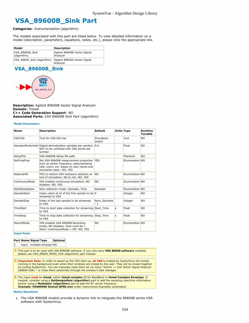
SystemVue - Algorithm Design Library
334
VSA_89600B_Sink PartCategories: Instrumentation (algorithm)
The models associated with this part are listed below. To view detailed information on amodel (description, parameters, equations, notes, etc.), please click the appropriate link.
Model Description
VSA_89600B_Sink(algorithm)
Agilent 89600B Vector SignalAnalyzer
VSA_89600_Sink (algorithm) Agilent 89600A Vector SignalAnalyzer
VSA_89600B_Sink
Description: Agilent 89600B Vector Signal AnalyzerDomain: TimedC++ Code Generation Support: NOAssociated Parts: VSA 89600B Sink Part (algorithm)
Model Parameters
Name Description Default Units Type RuntimeTunable
VSATitle Text for VSA title bar Simulationoutput
Text NO
SamplesPerSymbol Digital demodulation samples per symbol;NOT to be confused with VSA points persymbol
0.0 Float NO
SetupFile VSA 89600B Setup file path Filename NO
SetFreqProp Set VSA 89600B measurement propertiessuch as center frequency, span/samplingrate, zoom, ect. based on user inputs andsimulation data.: NO, YES
YES Enumeration NO
RestoreHW YES to restore VSA hardware selection atend of simulation; NO to not: NO, YES
NO Enumeration NO
ContinuousMode YES enables continuous simulation; NOdisables: NO, YES
NO Enumeration NO
StartStopOption Sink collection mode: Samples, Time Samples Enumeration NO
SampleStart Index (start at 0) of the first sample to bestreamed to VSA
0 Integer NO
SampleStop Index of the last sample to be streamedto VSA
Num_Samples- 1
Integer NO
TimeStart Time to start data collection for streamingto VSA
Start_Time s Float NO
TimeStop Time to stop data collection for streamingto VSA
Stop_Time s Float NO
RecordMode YES enables VSA 89600B Recordingmode; NO disables; Stop must be >Start, ContinuousMode = NO: NO, YES
NO Enumeration NO
Input Ports
Port Name Signal Type Optional
1 input multiple anytype NO
This part is to be used with VSA 89600B software. If you only have VSA 89600 software installed,please use VSA_89600_MIMO_Sink (algorithm) part instead.
Important Note: In order to speed up the VSA start-up, all VSA's created by SystemVue will remainrunning in the background even when their windows are closed by the user. They will be closed togetheron exiting SystemVue. You can manually close them all via menu *Action -> Exit Vector Signal Analyzer(89600 VSA) * or close them selectively through the window's task manager.
The input must be timed, either timed complex IQ for BaseBand or timed Complex Envelope. Ifneeded, consider using a SetSampleRate (algorithm) part to add the sampling rate/time informationand/or using a Modulator (algorithm) part to add the RF carrier frequency.Example: VSA89600 Demod QPSK.wsv under Instruments Examples (examples)
Notes/Equations
The VSA 89600B models provide a dynamic link to integrate the 89600B series VSA1.software with SystemVue.
SystemVue - Algorithm Design Library
335
Before using this model, the VSA89600B software must be installed. Download VSA 89600Bsoftware .For 89600B analyzer reference information, example measurements, or a getting startedvideo, access Help or choose Start -> Programs -> Agilent 89600B VSA -> Help.
The VSA_89600_Sink model provides a stream interface where you can input2.digitized waveforms directly from SystemVue to 89600-series VSA software withoutusing the 89600-series hardware. The full functionality of the 89600B analyzer isavailable to analyze and display the SystemVue signal.The SamplesPerSymbol parameter provides a convenient way to set the analyzer's3.Symbol Rate. This is different from the analyzer's Points/Symbol parameter, whichadjusts the analyzer's interpolation of demodulated data. SamplesPerSymbol takesprecedence over the Symbol Rate in the setup file, if a SetupFile is specified.The analyzer's digital demodulation algorithm limits the analyzer's span to a4.maximum of 15.625 times the Symbol Rate. This, plus the analyzer's maximumdecimation rate, places a lower limit on the Symbol Rate.The SetupFile parameter can be used to recall a VSA setup file automatically during5.simulation start-up. The VSA measurement setup file, SetupFile, is saved from theVSA application file menu, File -> Save -> Save Setup. To refine an existingSetupFile, you can modify the VSA application while simulating and then save thesetup file before restarting the simulation.
Note that once the mouse cursor is in SetupFile parameter's field, on the bottom left of theparameter setup window, a Browse... button is available and clicking it will open a file browser.
Triggering is not available in the 89600B when the input is from a simulation.6.If SetFreqProp = NO, the VSA's measurement center frequency, span, and zoom7.mode are left unchanged (except that these are loaded from a setup file, ifSetupFile is specified). If SetFreqProp = YES, the VSA's measurement centerfrequency, span, and zoom parameters is set to those of the simulation, overridingthose in the setup file, if specified.Unless a setup file is specified, the VSA application begins the simulation with its8.previous setup, with a few modifications dictated by the simulation. This settingenables for continuity of the VSA setup between simulations. RestoreHW = YES caninterfere with this. This continuity means that the initial VSA application setup can beimportant when a setup file is not specified. This includes the Hardware Setup.Starting a simulation in a known state, such as a preset state, can resolve some VSAinitialization problems. The VSA can be preset in various ways under File -> Preseton the VSA application. The Simulate Hardware selection under Hardware ->Utilities can be a useful starting point.If RestoreHW = NO (default), the VSA application remains in its Stream hardware9.setup at the end of a simulation. It can be returned to using other VSA hardwaresetups through the Hardware -> Utilities menu on the VSA application.If RestoreHW = YES, the hardware setup is saved at the beginning of the10.simulation and then restored at the end of the simulation. Since some measurementsetups change when the hardware setup changes, this setting can interfere with thecontinuity between simulations as described in previous note. In general, settingRestoreHW to NO or specifying SetupFile can have the least problems.One need for RestoreHW = YES is when changing between simulations where aVSA with the same Instance Name is used as a source in one simulation and a sink inanother and the VSA instance is not closed between the simulations. In this case, thesink VSA restores the source hardware setting at the end of the simulation.Otherwise, the VSA is left configured with Stream hardware and does not functioncorrectly as a source. The same problem arises if you would like to alternate betweenusing the same running VSA instance as a sink in a simulation and then would like tomake hardware based measurements.Set ContinuousMode to "YES" if you want the simulation to run indefinitely. You11.can always click the Stop button in the simulation progress display window to stopthe simulation.When RecordMode = YES (i.e., Time Capture mode, which is available only when12.ContinuousMode = NO), the 89600B Record buffer may need additional settlingpoints under some conditions, such as when the span is reduced (by lowering thesampling rate for example). (Note that the recording file is specified via the VSA89600B SW's menu "Input -> Recording ...").Multiple VSA_89600B_Sink components can be active in a simulation and you can13.configure each one independentlyWhen a simulation that contains an active VSA_89600B_Sink component starts, it14.attaches to a running 89600B whose title begins with the component's instancename. If no such 89600B instance is found, a new 89600B is created, and its title isset to the associated component's instance name and VSATitle text.
Important Links
Download latest VSA SW with 14 day trial license from Agilent Technologies1.If you did NOT install the Agilent IO library during the VSA SW installation, you can also download2.Agilent IO Library yourself.

SystemVue - Algorithm Design Library
336
VSA_89600B_Source PartCategories: Instrumentation (algorithm)
The models associated with this part are listed below. To view detailed information on amodel (description, parameters, equations, notes, etc.), please click the appropriate link.
Model Description
VSA_89600B_Source(algorithm)
Agilent 89600B Vector SignalAnalyzer
VSA_89600_Source (algorithm) Agilent 89600A Vector SignalAnalyzer
VSA_89600B_Source
Description: Agilent 89600B Vector Signal AnalyzerDomain: TimedC++ Code Generation Support: NOAssociated Parts: VSA 89600B Source Part (algorithm)
Model Parameters
Name Description Default Units Type RuntimeTunable
Range
VSATitle Text for VSA title bar Simulationoutput
Text NO
Pause Pause for user to manually adjustVSA settings: NO, YES
NO Enumeration NO
OutputType Output port type: Timed,Frequency, Demod Errors, ComplexScalar, Float Scalar, Integer Scalar
Timed Enumeration NO
VSATrace VSA trace that will supply data.: A,B, C, D, E, F, G, H
B Enumeration NO
RepeatData VSA hardware measurementcontrol: Repeat, Reacquire, Singlepass
Repeat Enumeration NO
TStep Simulation time step 0 s Float NO
SetupFile Name of setup file to recall intoVSA
Filename NO
SetupUse VSA setup file recall control:Always, Once, No
Always Enumeration NO
RecordingFile Name of recording file to recall intoVSA to be played back
Filename NO
AutoCapture Capture VSA input data at start-up:NO, YES
NO Enumeration NO
DefaultHardware Use VSA default hardwareconfiguration: NO, YES
NO Enumeration NO
FrequencySpan If non-zero, set the frequencyspan.
0 Hz Float NO [0:∞)
SetCenterFrequency Controls the CenterFrequencyparameter.: NO, YES
NO Enumeration NO
CenterFrequency Center frequency 0 Hz Float NO (-∞:∞)
Range If non-zero and RecordingFile notset, set the range.
0 V Float NO [0:∞)
RecordingLength If non-zero and RecordingFile notset, this parameter set therecording length.
0 s Float NO [0:∞)
Output Ports
Port Name Description Signal Type Optional
1 out Measurement data anytype NO
2 gap VSA input data gapsignal
int NO
This part is to be used with VSA 89600B software. If you only have VSA 89600 software installed,please use VSA_89600_Source (algorithm) part instead.

SystemVue - Algorithm Design Library
337
Important Note: In order to speed up the VSA start-up, all VSA's created by SystemVue will remainrunning in the background even when their windows are closed by the user. They will be closed togetheron exiting SystemVue. You can manually close them all via menu *Action -> Exit Vector Signal Analyzer(89600 VSA) * or close them selectively through the window's task manager.
Measurement data from VSA 89600B streams out of Port 1
Example: VSA89600 Recall QAM512 Data.wsv under Instruments Examples(examples)
Notes/Equations
The VSA 89600B models provide a dynamic link to integrate the 89600B series VSA1.software with SystemVue.Before using this model, the VSA 89600B software must be installed. Download VSA2.89600B software .For 89600B analyzer reference information, example measurements, or a getting3.started video, access Help or choose Start -> Programs -> Agilent 89600B VSA-> Help.The VSA_89600B_Source model transfers measurement data from the 89600B4.Vector Signal Analyzer. The model outputs different amounts and types of datadepending on OutputType, as described in detail under the OutputType parameter.Measurements can be acquired from any 89600 trace and are transferred in raw5.(unformatted) state.The VSATitle parameter sets the title in the 89600B window title bar.6.The Pause parameter controls the 89600 start-up sequence:7.
When Pause = YES, the simulation displays a message dialog and pause beforeacquiring measurement data from the 89600B. This allows you to configure the89600B before pressing the OK button to proceed.
The OutputType parameter establishes the configuration of the model's output data8.port.
ImportantThe data type of the 89600B trace selected by VSATrace must be compatible with the outputtype.
Timed - Timed data is output at the 89600B center frequency and timestep(refer to TStep for detail). The data can be complex or baseband, depending onthe 89600 zoom state. Requires time domain measurements from the 89600B.Frequency - Spectrum data is output as pairs of complex numbers. The firstnumber is the real frequency (the imaginary part is zero), and the secondnumber is the complex voltage at that frequency. You can connect a to theVSA_89600B_Source data port to separate the signal. Requires frequencydomain measurements from the 89600B. Example 89600B trace data type:Spectrum.Demod Errors - Demodulation error data is output as sets of floating-point(real) values. The number of values and required 89600B configuration varywith demod type. See note 20.Complex Scalar - Complex numbers are output. If the 89600B measurementdata is real-valued, the imaginary part of the output values is zero. Example89600B trace data type: "Error Vector Time" in Digital Demod mode.Float Scalar - Floating point numbers are output. Requires real-valued 89600Bmeasurement data. Example 89600B trace data type: "IQ Mag Error" in DigitalDemod mode.Integer Scalar - Integer numbers are output. Requires real-valued 89600measurement data. Useful for sourcing demodulation symbols when the 89600Btrace data type is Syms/Errs.
The VSATrace parameter specifies which 89600B trace provides measurement data.9.The RepeatData parameter controls the transfer of data from the 89600B during10.hardware-based measurement.
When RepeatData = Single pass, the model supplies data from a singlemeasurement. The Repeat option acquires a single measurement andrepetitively sources it into the simulation. Reacquire repeatedly acquires andsources new measurements. Note that in the Repeat and Reacquire modes time-based data is not continuous across measurements.
When 89600B input is from a recording the RepeatData setting is ignored. Refer to note 19 forinformation on operation with recordings.
The TStep parameter can be used to specify a target timestep when sourcing timed11.data. The model trys to adjust the 89600B's span to achieve the requested step sizevia resampling. If the 89600B cannot be set to the required span, a warning messageis output to the status window.The SetupFile parameter can be used to recall automatically a VSA setup file during12.simulation start-up. The VSA measurement setup file, SetupFile, is saved from theVSA application file menu, File -> Save -> Save Setup. To refine an existingSetupFile, you can modify the VSA application while simulating and then save thesetup file before restarting the simulation. If Pause = YES, the setup file is loadedbefore the Pause dialog is displayed.
Note that once the mouse cursor is in SetupFile parameter's field, on the bottom left of theparameter setup window, a Browse... button is available and clicking it will open a file browser.

SystemVue - Algorithm Design Library
338
The SetupUse parameter specifies when an 89600B setup file (specified in the13.SetupFile parameter) is recalled. Options are:
Always - Recall setup file on every simulation run.Once - Recall setup file only when 89600B is started.No - Do not recall setup file.
The RecordingFile parameter can be used to recall automatically a recording into14.the 89600 during simulation start-up. #* If Pause = YES, the recording file isloaded before the Pause dialog is displayed.
Use the Browse... button to open the file browser in the same way as handling SetupFile.
The AutoCapture parameter can be set to YES to have the 89600B automatically15.initiate a capture recording of hardware input data at the beginning of a simulation.When the capture is complete, the model begins sourcing the recorded data. Time-based measurements is continuous (note 19). Recording length can be controlled viaan 89600B setup file.The DefaultHardware parameter can be set to YES to have the 89600 automatically16.select an appropriate hardware configuration. Otherwise, the 89600B uses previoushardware settings. Note that when a source 89600B reuses the same running89600B instance that was used by a sink 89600, it can be left set up with Streaminput hardware. This problem can be solved via the RestoreHW parameter of theVSA_89600B_Sink (algorithm) component.Each 89600B measurement produces a block of data points, which are pipelined to17.the simulation. As a result, simulation plots typically lag 89600B traces. The numberof points in a block varies with 89600B measurement type and configuration. Forreference, the block size is output to the status window during startup. This value canbe useful when configuring other components (for example, plot persistence andupdate size). Also, any change in block size during simulation is logged in the statuswindow.The units associated with transferred 89600B data are output to the status window18.during startup. Unless otherwise indicated, values are peak units.To avoid transfer of overlapped measurement data, the 89600B's maximum overlap19.for averaging off is set to zero when a simulation starts.If the model detects a change to one of the following 89600B settings while sourcing20.data, the model disconnects from the 89600B.
Input data sourceDemodulator configurationData type of the trace supplying measurements (VSATrace)Sweep modeCenter frequency (for timed output)Timestep size (for timed output)
The recommended practice is to use the Pause and/or SetupFile options to pre-configure the89600B.
When a simulation that contains an active VSA_89600B_Source component starts, it21.attaches to a running 89600B whose title begins with the component's instancename. If no such 89600B instance is found, a new 89600B is created, and its title isset to the associated component's instance name and VSATitle text.When 89600B input is from a recording, the model steps through the recording,22.transferring all measurements. 89600B recording playback properties can be used tocontrol start/stop points and looping. In this mode time-based data are continuous,with the exception of wrapped values when a playback loop occurs.Demodulation Error/Summary information is available by configuring the trace data.23.
For details on results available, please refer to the following:89600B help index topic symbol table and look for the demodulation format of interest.The demod formats available depend on 89600B licensing (For example, Digital Demodrequires option AYA, and cdma2000 requires option B7.)The error summary data and the numbering for each demodulation format are documented intables in the 89600B help documentation (look in the index under demod errors).Also note that some demodulation formats include several of these tables. The table valuesare output in a fixed sequence, which can be different from the order seen on the 89600Bdisplay.The number of output error values depends on the configuration.The easiest way to get an individual error value is to place a DownSample component in serieswith the VSA 89600B Source output.For example, consider the list of Digital Demod error items. The DownSample Factorparameter would be set to the number of error values (21). To select EVM, the Phaseparameter would be set to 20 (EVM position in the list subtracted from 21).When OutputType is Integer Scalar and trace data is configured to one of the above types(Syms/Errs, for example), the module sources demodulation symbols.
The gap output port emits a 1 when there is a discontinuity in 89600B input data.24.Otherwise it emits 0.Multiple VSA_89600B_Source components can be active in a simulation.25.When both VSA_89600B_Source and VSA_89600B_Sink (algorithm) components26.are present in a design, configuring the VSA_89600B_Sink (algorithm) for 0%time record overlap minimizes the effect of gaps in source data.The VSA_89600B_Source component does not handle averaged measurements as a27.special case; each 89600B analyzer trace update is output to the simulation. Thedefault 89600B analyzer average setup has Fast Average disabled, so the traces areupdated each time new measurement results are added to the average, starting withthe first measurement.

SystemVue - Algorithm Design Library
339
To force only the final, fully averaged result to be output to the simulation, select28.MeasSetup -> Average on the 89600B analyzer and check both the Fast Averageand the Same as Count check boxes. This prevents the analyzer from updating thescreen until the selected number of measurements have been averaged together.
Additional Important Links
Download latest VSA SW with 14 day trial license from Agilent Technologies1.If you did NOT install the Agilent IO library during the VSA SW installation, you can also download2.Agilent IO Library yourself.

SystemVue - Algorithm Design Library
340
VSA_89600_MIMO_Sink PartCategories: Instrumentation (algorithm)
The models associated with this part are listed below. To view detailed information on amodel (description, parameters, equations, notes, etc.), please click the appropriate link.
Model Description
VSA_89600_MIMO_Sink(algorithm)
Agilent 89600A Vector SignalAnalyzer
VSA_89600_MIMO_Sink
Description: Agilent 89600A Vector Signal Analyzer for MIMO ApplicationsDomain: TimedC++ Code Generation Support: NOAssociated Parts: VSA 89600B MIMO Sink Part (algorithm)
Model Parameters
Name Description Default Units Type RuntimeTunable
VSATitle Text for VSA title bar MIMOSimulationoutput
Text NO
NumberOfChannels Number of channels.: 2 channels, 3channels, 4 channels
2 channels Enumeration NO
SamplesPerSymbol Digital demodulation samples persymbol; NOT to be confused with VSApoints per symbol
0.0 Float NO
SetupFile Name of measurement setup file torecall
Filename NO
SetFreqProp Set VSA 89600 measurement propertiessuch as center frequency, span/samplingrate, zoom, ect. based on user inputsand simulation data.: NO, YES
YES Enumeration NO
RestoreHW YES to restore VSA hardware selectionat end of simulation; NO to not: NO, YES
NO Enumeration NO
ContinuousMode YES enables continuous simulation; NOdisables: NO, YES
NO Enumeration NO
Start Sample number to start measuring 0 Integer NO
Stop Sample number to stop measuring Num_Samples -1
Integer NO
RecordMode YES enables VSA 89600 Recordingmode; NO disables; Stop must be >Start, ContinuousMode = NO: NO, YES
NO Enumeration NO
Important Note: Starting from SystemVue2009.08 release, in order to speed up the VSA start-up, allVSA's created by SystemVue will remain running in the background even when their windows are closedby the user. They will be closed together on exiting SystemVue. You can manually close them all via menu*Action -> Exit Vector Signal Analyzer (89600 VSA) * or close them selectively through the window's taskmanager.
VSA 89600 MIMO Sink is for MIMO applications only. It is designed to stream the time domain datafrom multiple simulated RF antennas into VSA SW to be processed by it.
To stream single antenna data into VSA SW, please use VSA_89600_Sink (algorithm).
VSA MIMO Sink UI Properties
If desired, click the Advanced Options ... button on the bottom left corner of VSA MIMO SinkProperties UI to view the parameter list. The mapping between the parameters in the parameter list andthe setup controls shown in the Graphic User Interface described above should be straightforward.
Most of the setup controls in the User Interface is self explanatory. In the following weonly cover a few key setup controls.
Number of Channels Currently only up to 4 MIMO channels are supported.1.Sample start & Sample Stop Defines the range of simulation data that VSA MIMO2.Sink should capture and process. To have it capture and process simulation data non-stop, check the Free-running simulation box.VSA Setup File: Browse the VSA setup file that configures how to process the data3.
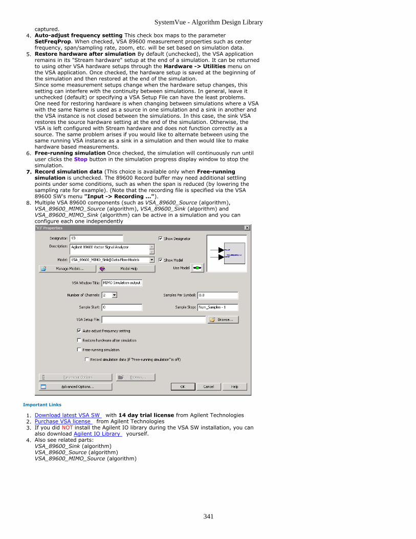
SystemVue - Algorithm Design Library
341
captured.Auto-adjust frequency setting This check box maps to the parameter4.SetFreqProp. When checked, VSA 89600 measurement properties such as centerfrequency, span/sampling rate, zoom, etc. will be set based on simulation data.Restore hardware after simulation By default (unchecked), the VSA application5.remains in its "Stream hardware" setup at the end of a simulation. It can be returnedto using other VSA hardware setups through the Hardware -> Utilities menu onthe VSA application. Once checked, the hardware setup is saved at the beginning ofthe simulation and then restored at the end of the simulation.Since some measurement setups change when the hardware setup changes, thissetting can interfere with the continuity between simulations. In general, leave itunchecked (default) or specifying a VSA Setup File can have the least problems.One need for restoring hardware is when changing between simulations where a VSAwith the same Name is used as a source in one simulation and a sink in another andthe VSA instance is not closed between the simulations. In this case, the sink VSArestores the source hardware setting at the end of the simulation. Otherwise, theVSA is left configured with Stream hardware and does not function correctly as asource. The same problem arises if you would like to alternate between using thesame running VSA instance as a sink in a simulation and then would like to makehardware based measurements.Free-running simulation Once checked, the simulation will continuously run until6.user clicks the Stop button in the simulation progress display window to stop thesimulation.Record simulation data (This choice is available only when Free-running7.simulation is unchecked. The 89600 Record buffer may need additional settlingpoints under some conditions, such as when the span is reduced (by lowering thesampling rate for example). (Note that the recording file is specified via the VSA89600 SW's menu "Input -> Recording ...").Multiple VSA 89600 components (such as VSA_89600_Source (algorithm),8.VSA_89600_MIMO_Source (algorithm), VSA_89600_Sink (algorithm) andVSA_89600_MIMO_Sink (algorithm) can be active in a simulation and you canconfigure each one independently
Important Links
Download latest VSA SW with 14 day trial license from Agilent Technologies1.Purchase VSA license from Agilent Technologies2.If you did NOT install the Agilent IO library during the VSA SW installation, you can3.also download Agilent IO Library yourself.Also see related parts:4.VSA_89600_Sink (algorithm)VSA_89600_Source (algorithm)VSA_89600_MIMO_Source (algorithm)

SystemVue - Algorithm Design Library
342
VSA_89600_MIMO_Source PartCategories: Instrumentation (algorithm)
The models associated with this part are listed below. To view detailed information on amodel (description, parameters, equations, notes, etc.), please click the appropriate link.
Model Description
VSA_89600_MIMO_Source(algorithm)
Agilent 89600A Vector Signal Analyzer for MIMO Applications
VSA_89600_MIMO_Source
Description: Agilent 89600A Vector Signal Analyzer for MIMO ApplicationsDomain: TimedC++ Code Generation Support: NOAssociated Parts: VSA 89600B MIMO Source Part (algorithm)
Model Parameters

SystemVue - Algorithm Design Library
343
Name Description Default Units Type RuntimeTunable
Range
VSATitle Text for VSA title bar Simulationsource
Text NO
RepeatData VSA hardware measurementcontrol: Repeat, Reacquire,Single pass
Reacquire Enumeration NO
Pause Pause for user to manuallyadjust VSA settings: NO, YES
NO Enumeration NO
SetupFile Name of setup file to recall intoVSA
Filename NO
SetupUse VSA setup file recall control:Always, Once, No
Always Enumeration NO
SampleRateOption Set the sample rate for theoutput signals: From Traces,User Specified
From Traces Enumeration NO
SampleRate Sample rate sepcified by user Sample_Rate Hz Float NO
NumberOfAntennas Number of receiver attennas: 2Antennas, 3 Antennas, 4Antennas
2 Antennas Enumeration NO
Antenna1_Trace VSA trace that will supply the1st antenna's time domaintrace.: A, B, C, D, E, F
A Enumeration NO
Antenna2_Trace VSA trace that will supply the2nd antenna's time domaintrace.: A, B, C, D, E, F
B Enumeration NO
Antenna3_Trace VSA trace that will supply the3rd antenna's time domaintrace.: A, B, C, D, E, F
C Enumeration NO
Antenna4_Trace VSA trace that will supply the3rd antenna's time domaintrace.: A, B, C, D, E, F
D Enumeration NO
RecordingFile Name of recording file to recallinto VSA to be played back
Filename NO
AutoCapture Capture VSA input data atstart-up: NO, YES
NO Enumeration NO
ShowAdvancedParams Show advanced parameters:NO, YES
NO Enumeration NO
DefaultHardware Use VSA default hardwareconfiguration: NO, YES
NO Enumeration NO
SetFrequencySpan Enables the FrequencySpanparameter.: NO, YES
NO Enumeration NO
FrequencySpan If non-zero, set the frequencyspan.
0 Hz Float NO [0:∞)
SetCenterFrequency Enables the CenterFrequencyparameter.: NO, YES
NO Enumeration NO
CenterFrequency Center frequency 0 Hz Float NO (-∞:∞)
SetRange Enables the Range parameter.:NO, YES
NO Enumeration NO
Range If non-zero and RecordingFilenot set, set the range.
0 V Float NO [0:∞)
RecordingLength If non-zero and RecordingFilenot set, this parameter set therecording length.
0 s Float NO [0:∞)
GapOut Enable outputtingmeasurement Gap flag.: NO,YES
NO Enumeration NO
Important Note: Starting from SystemVue2009.08 release, in order to speed up the VSA start-up, allVSA's created by SystemVue will remain running in the background even when their windows are closedby the user. They will be closed together on exiting SystemVue. You can manually close them all via menu*Action -> Exit Vector Signal Analyzer (89600 VSA) * or close them selectively through the window's taskmanager.
VSA 89600 MIMO Source is for MIMO applications only. It is designed to retrieve the time domaindata of multiple RF sources captured by VSA SW and stream them into simulation for measurements suchas Bit Error Rate measurement.
To retrieve other measurement data (e.g. spectrum) from VSA SW, please use VSA_89600_Source(algorithm).
VSA MIMO Main Properties
VSA Window Title If the VSA SW's window is displayed (by check the Pause VSA1.box under the VSA MIMO Advanced Properties tab), this will be the title for thatwindow.Number of Antennas Controls how many RF signals are concurrently captured and2.streamed into the simulator from the VSA SW. Note how this parameter changes thecontent grouped under the "Outputs" and how it also changes the number of outputpins on the little icon in the top right corner of this window.
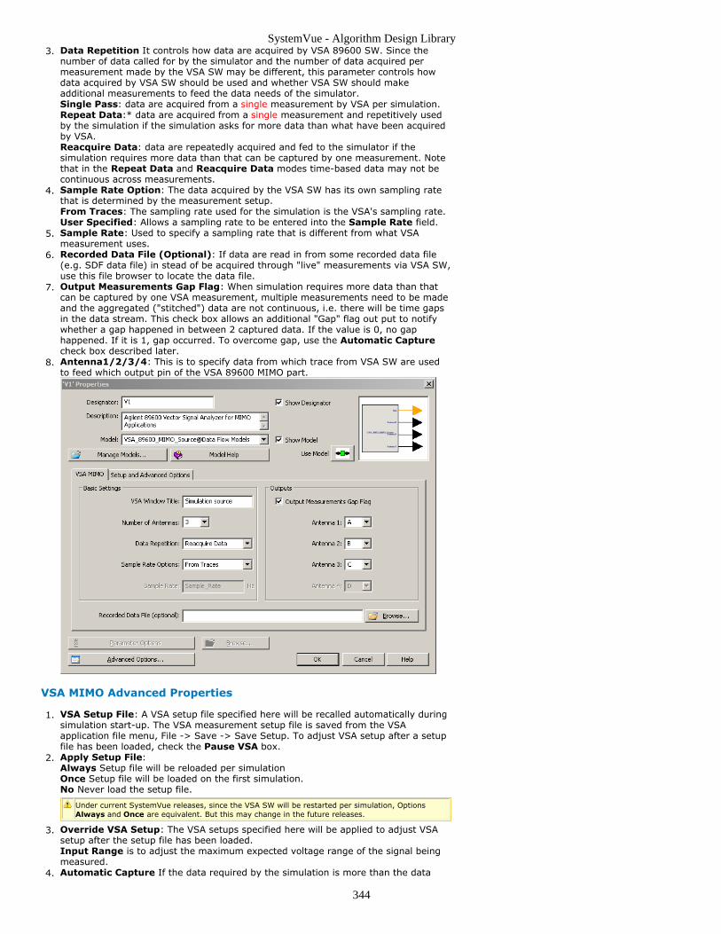
SystemVue - Algorithm Design Library
344
Data Repetition It controls how data are acquired by VSA 89600 SW. Since the3.number of data called for by the simulator and the number of data acquired permeasurement made by the VSA SW may be different, this parameter controls howdata acquired by VSA SW should be used and whether VSA SW should makeadditional measurements to feed the data needs of the simulator.Single Pass: data are acquired from a single measurement by VSA per simulation.Repeat Data:* data are acquired from a single measurement and repetitively usedby the simulation if the simulation asks for more data than what have been acquiredby VSA.Reacquire Data: data are repeatedly acquired and fed to the simulator if thesimulation requires more data than that can be captured by one measurement. Notethat in the Repeat Data and Reacquire Data modes time-based data may not becontinuous across measurements.Sample Rate Option: The data acquired by the VSA SW has its own sampling rate4.that is determined by the measurement setup.From Traces: The sampling rate used for the simulation is the VSA's sampling rate.User Specified: Allows a sampling rate to be entered into the Sample Rate field.Sample Rate: Used to specify a sampling rate that is different from what VSA5.measurement uses.Recorded Data File (Optional): If data are read in from some recorded data file6.(e.g. SDF data file) in stead of be acquired through "live" measurements via VSA SW,use this file browser to locate the data file.Output Measurements Gap Flag: When simulation requires more data than that7.can be captured by one VSA measurement, multiple measurements need to be madeand the aggregated ("stitched") data are not continuous, i.e. there will be time gapsin the data stream. This check box allows an additional "Gap" flag out put to notifywhether a gap happened in between 2 captured data. If the value is 0, no gaphappened. If it is 1, gap occurred. To overcome gap, use the Automatic Capturecheck box described later.Antenna1/2/3/4: This is to specify data from which trace from VSA SW are used8.to feed which output pin of the VSA 89600 MIMO part.
VSA MIMO Advanced Properties
VSA Setup File: A VSA setup file specified here will be recalled automatically during1.simulation start-up. The VSA measurement setup file is saved from the VSAapplication file menu, File -> Save -> Save Setup. To adjust VSA setup after a setupfile has been loaded, check the Pause VSA box.Apply Setup File:2.Always Setup file will be reloaded per simulationOnce Setup file will be loaded on the first simulation.No Never load the setup file.
Under current SystemVue releases, since the VSA SW will be restarted per simulation, OptionsAlways and Once are equivalent. But this may change in the future releases.
Override VSA Setup: The VSA setups specified here will be applied to adjust VSA3.setup after the setup file has been loaded.Input Range is to adjust the maximum expected voltage range of the signal beingmeasured.Automatic Capture If the data required by the simulation is more than the data4.

SystemVue - Algorithm Design Library
345
held by each VSA measurement (i.e. its corresponding trace(s)), multiplemeasurements are required to provide the required number of data and in general, itwill create measurement gaps that will distort the final measurement results such asBit Error Rate (BER). If gap such introduced is not tolerable by the application suchas BER, the solution is to have the VSA SW record enough data for the simulationthrough one single continuous measurement then feed these recorded data to thesimulation. This check box is used to achieve this. You can leave the RecordingLength as 0 if the setup file already has a long recording length specified.Use Default Hardware If checked, it will have the 89600 automatically select an5.appropriate hardware configuration. Otherwise, the 89600 uses previous hardwareselections. Note that when a source 89600 works together with a VSA_89600_Sink(algorithm) part, it can be left set up with Stream input hardware. This problem canbe solved via the RestoreHW parameter of the VSA_89600_Sink (algorithm)component..Pause VSA: If you need to make some modifications to the VSA setup after loading6.a VSA setup file bu tbefore simulation starts, you can check this check box so thatthe VSA window will be brought up after the setup file has been loaded to allow youto make those adjustments.
If desired, click the Advanced Options ... button on the bottom left corner of VSA MIMO MainProperties to view the parameter list. The mapping between the parameters in the parameter list and thesetup controls shown in the 2 Graphic User Interfaces described above should be straightforward.
Important Links
Download latest VSA SW with 14 day trial license from Agilent Technologies1.Purchase VSA license from Agilent Technologies2.If you did NOT install the Agilent IO library during the VSA SW installation, you can3.also download Agilent IO Library yourself.Also see related parts:4.VSA_89600_Sink (algorithm)VSA_89600_Source (algorithm)

SystemVue - Algorithm Design Library
346
VSA_89600_Sink PartCategories: Instrumentation (algorithm)
The models associated with this part are listed below. To view detailed information on amodel (description, parameters, equations, notes, etc.), please click the appropriate link.
Model Description
VSA_89600_Sink(algorithm)
Agilent 89600 Vector Signal Analyzer
VSA_89600_Sink
Description: Agilent 89600A Vector Signal AnalyzerDomain: TimedC++ Code Generation Support: NOAssociated Parts: VSA 89600B Sink Part (algorithm)
Model Parameters
Name Description Default Units Type RuntimeTunable
VSATitle Text for VSA title bar Simulationoutput
Text NO
SamplesPerSymbol Digital demodulation samples per symbol;NOT to be confused with VSA points persymbol
0.0 Float NO
SetupFile Name of measurement setup file to recall Filename NO
SetFreqProp Set VSA 89600 measurement propertiessuch as center frequency, span/samplingrate, zoom, ect. based on user inputs andsimulation data.: NO, YES
YES Enumeration NO
RestoreHW YES to restore VSA hardware selection atend of simulation; NO to not: NO, YES
NO Enumeration NO
ContinuousMode YES enables continuous simulation; NOdisables: NO, YES
NO Enumeration NO
Start Sample number to start measuring 0 Integer NO
Stop Sample number to stop measuring Num_Samples- 1
Integer NO
RecordMode YES enables VSA 89600 Recording mode;NO disables; Stop must be > Start,ContinuousMode = NO: NO, YES
NO Enumeration NO
Input Ports
Port Name Signal Type Optional
1 input multiple anytype NO
Important Note: Starting from SystemVue2009.08 release, in order to speed up the VSA start-up, allVSA's created by SystemVue will remain running in the background even when their windows are closedby the user. They will be closed together on exiting SystemVue. You can manually close them all via menu*Action -> Exit Vector Signal Analyzer (89600 VSA) * or close them selectively through the window's taskmanager.
The input must be timed, either timed complex IQ for BaseBand or timed Complex Envelope. Ifneeded, consider using a SetSampleRate (algorithm) part to add the sampling rate/time informationand/or using a Modulator (algorithm) part to add the RF carrier frequency.Example: VSA89600 Demod QPSK.wsv under Instruments Examples (examples)
Notes/Equations
The VSA_89600 models provide a dynamic link to integrate the 89600 series VSA1.software with SystemVue.
Before using this model, the VSA89600 software must be installed. The VSA 89600 softwarecan be downloaded from http://www.agilent.com/find/89600 .For 89600 analyzer reference information, example measurements, or a getting started video,access Help or choose Start -> Programs -> Agilent 89600 VSA -> Help.
The VSA_89600_Sink model provides a stream interface where you can input2.digitized waveforms directly from SystemVue to 89600-series VSA software withoutusing the 89600-series hardware. The full functionality of the 89600 analyzer isavailable to analyze and display the SystemVue signal.The SamplesPerSymbol parameter provides a convenient way to set the analyzer's3.Symbol Rate. This is different from the analyzer's Points/Symbol parameter, which

SystemVue - Algorithm Design Library
347
adjusts the analyzer's interpolation of demodulated data. SamplesPerSymbol takesprecedence over the Symbol Rate in the setup file, if a SetupFile is specified.The analyzer's digital demodulation algorithm limits the analyzer's span to a4.maximum of 15.625 times the Symbol Rate. This, plus the analyzer's maximumdecimation rate, places a lower limit on the Symbol Rate.The SetupFile parameter can be used to recall a VSA setup file automatically during5.simulation start-up. The VSA measurement setup file, SetupFile, is saved from theVSA application file menu, File -> Save -> Save Setup. To refine an existingSetupFile, you can modify the VSA application while simulating and then save thesetup file before restarting the simulation.
Note that once the mouse cursor is in SetupFile parameter's field, on the bottom left of theparameter setup window, a Browse... button is available and clicking it will open a file browser.
Triggering is not available in the 89600 when the input is from a simulation.6.If SetFreqProp = NO, the VSA's measurement center frequency, span, and zoom7.mode are left unchanged (except that these are loaded from a setup file, ifSetupFile is specified). If SetFreqProp = YES, the VSA's measurement centerfrequency, span, and zoom parameters is set to those of the simulation, overridingthose in the setup file, if specified.Unless a setup file is specified, the VSA application begins the simulation with its8.previous setup, with a few modifications dictated by the simulation. This settingenables for continuity of the VSA setup between simulations. RestoreHW = YES caninterfere with this. This continuity means that the initial VSA application setup can beimportant when a setup file is not specified. This includes the Hardware Setup.Starting a simulation in a known state, such as a preset state, can resolve some VSAinitialization problems. The VSA can be preset in various ways under File -> Preseton the VSA application. The Simulate Hardware selection under Hardware ->Utilities can be a useful starting point.If RestoreHW = NO (default), the VSA application remains in its Stream hardware9.setup at the end of a simulation. It can be returned to using other VSA hardwaresetups through the Hardware -> Utilities menu on the VSA application.If RestoreHW = YES, the hardware setup is saved at the beginning of the10.simulation and then restored at the end of the simulation. Since some measurementsetups change when the hardware setup changes, this setting can interfere with thecontinuity between simulations as described in previous note. In general, settingRestoreHW to NO or specifying SetupFile can have the least problems.One need for RestoreHW = YES is when changing between simulations where aVSA with the same Instance Name is used as a source in one simulation and a sink inanother and the VSA instance is not closed between the simulations. In this case, thesink VSA restores the source hardware setting at the end of the simulation.Otherwise, the VSA is left configured with Stream hardware and does not functioncorrectly as a source. The same problem arises if you would like to alternate betweenusing the same running VSA instance as a sink in a simulation and then would like tomake hardware based measurements.Set ContinuousMode to "YES" if you want the simulation to run indefinitely. You11.can always click the Stop button in the simulation progress display window to stopthe simulation.When RecordMode = YES (i.e., Time Capture mode, which is available only when12.ContinuousMode = NO), the 89600 Record buffer may need additional settlingpoints under some conditions, such as when the span is reduced (by lowering thesampling rate for example). (Note that the recording file is specified via the VSA89600 SW's menu "Input -> Recording ...").Multiple VSA_89600_Sink components can be active in a simulation and you can13.configure each one independentlyWhen a simulation that contains an active VSA_89600_Sink component starts, it14.attaches to a running 89600 whose title begins with the component's instance name.If no such 89600 instance is found, a new 89600 is created, and its title is set to theassociated component's instance name and VSATitle text.
Important Links
Download latest VSA SW with 14 day trial license from Agilent Technologies1.Purchase VSA license from Agilent Technologies2.If you did NOT install the Agilent IO library during the VSA SW installation, you can also download3.Agilent IO Library yourself.

SystemVue - Algorithm Design Library
348
Commonly Seen Errors
Error Seen When Using Workspace Created on a Different Computer1.If you copy a workspace from a different computer, occasionally you might see the following error messages:"Cannot create the file C:\Documents and Settings\fxdit\My Documents\Agilent\89600VSA\Data\Recording.sdf.4088", recording file ...To fix this, you can either try to replace the VSA_89600_Sink used in the schematic/design with a new one, or simply addall the missing folders specified along the path C:\Documents and Settings\fxdit\My Documents\Agilent\89600VSA\Data.Error Seen When Using RecordMode2.When you set "RecordMode" to "YES" and you see the following Error writing to temporary file C:\Documents andSettings\fxdit\My Documents\Agilent\89600 VSA\Data\Recording.sdf.1234 complaint from VSA 89600 SW, it isvery likely you have copied the workspace (project) from somewhere else. To fix it, you can either try to replace theVSA_89600_Sink used in the schematic/design with a new one, or simply add all the missing folders specified along thepath C:\Documents and Settings\fxdit\My Documents\Agilent\89600 VSA\Data.

SystemVue - Algorithm Design Library
349
VSA_89600_Source PartCategories: Instrumentation (algorithm)
The models associated with this part are listed below. To view detailed information on amodel (description, parameters, equations, notes, etc.), please click the appropriate link.
Model Description
VSA_89600_Source(algorithm)
Agilent 89600A Vector SignalAnalyzer
VSA_89600_Source
Description: Agilent 89600A Vector Signal AnalyzerDomain: TimedC++ Code Generation Support: NOAssociated Parts: VSA 89600B Source Part (algorithm)
Model Parameters
Name Description Default Units Type RuntimeTunable
Range
VSATitle Text for VSA title bar Simulationsource
Text NO
Pause Pause for user to manually adjustVSA settings: NO, YES
NO Enumeration NO
OutputType Output port type: Timed,Frequency, Demod Errors, ComplexScalar, Float Scalar, Integer Scalar
Timed Enumeration NO
VSATrace VSA trace that will supply data.: A,B, C, D
B Enumeration NO
RepeatData VSA hardware measurementcontrol: Repeat, Reacquire, Singlepass
Repeat Enumeration NO
TStep Simulation time step 0 s Float NO
SetupFile Name of setup file to recall intoVSA
Filename NO
SetupUse VSA setup file recall control:Always, Once, No
Always Enumeration NO
RecordingFile Name of recording file to recall intoVSA to be played back
Filename NO
AutoCapture Capture VSA input data at start-up:NO, YES
NO Enumeration NO
DefaultHardware Use VSA default hardwareconfiguration: NO, YES
NO Enumeration NO
FrequencySpan If non-zero, set the frequencyspan.
0 Hz Float NO [0:∞)
SetCenterFrequency Controls the CenterFrequencyparameter.: NO, YES
NO Enumeration NO
CenterFrequency Center frequency 0 Hz Float NO (-∞:∞)
Range If non-zero and RecordingFile notset, set the range.
0 V Float NO [0:∞)
RecordingLength If non-zero and RecordingFile notset, this parameter set therecording length.
0 s Float NO [0:∞)
Output Ports
Port Name Description Signal Type Optional
1 out Measurement data anytype NO
2 gap VSA input data gapsignal
int NO
Important Note: Starting from SystemVue2009.08 release, in order to speed up the VSA start-up, allVSA's created by SystemVue will remain running in the background even when their windows are closedby the user. They will be closed together on exiting SystemVue. You can manually close them all via menu*Action -> Exit Vector Signal Analyzer (89600 VSA) * or close them selectively through the window's taskmanager.

SystemVue - Algorithm Design Library
350
In SystemVue2009.05 official release, we have taken out the multiple time domain traces (for MIMOapplications) support we introduced during SystemVue2009.05 Alpha. If you are using this feature, pleaseuse VSA 89600 MIMO Source Part (algorithm) instead.
Measurement data from VSA 89600 streams out of Port 1
Example: VSA89600 Recall QAM512 Data.wsv under Instruments Examples(examples)
Notes/Equations
The VSA_89600 models provide a dynamic link to integrate the 89600 series VSA1.software with SystemVue.Before using this model, the VSA 89600 software must be installed. The VSA 896002.software can be downloaded from http://www.agilent.com/find/89600 .For 89600 analyzer reference information, example measurements, or a getting3.started video, access Help or choose Start -> Programs -> Agilent 89600 VSA -> Help.The VSA_89600_Source model transfers measurement data from the 89600 Vector4.Signal Analyzer. The model outputs different amounts and types of data dependingon OutputType, as described in detail under the OutputType parameter.Measurements can be acquired from any 89600 trace and are transferred in raw5.(unformatted) state.The VSATitle parameter sets the title in the 89600 window title bar.6.The Pause parameter controls the 89600 start-up sequence:7.
When Pause = YES, the simulation displays a message dialog and pause beforeacquiring measurement data from the 89600. This allows you to configure the89600 before pressing the OK button to proceed.
The OutputType parameter establishes the configuration of the model's output data8.port.
ImportantThe data type of the 89600 trace selected by VSATrace must be compatible with the outputtype.
Timed - Timed data is output at the 89600 center frequency and timestep (referto TStep for detail). The data can be complex or baseband, depending on the89600 zoom state. Requires time domain measurements from the 89600.Frequency - Spectrum data is output as pairs of complex numbers. The firstnumber is the real frequency (the imaginary part is zero), and the secondnumber is the complex voltage at that frequency. You can connect a to theVSA_89600_Source data port to separate the signal. Requires frequency domainmeasurements from the 89600. Example 89600 trace data type: Spectrum.Demod Errors - Demodulation error data is output as sets of floating-point(real) values. The number of values and required 89600 configuration vary withdemod type. See note 20.Complex Scalar - Complex numbers are output. If the 89600 measurementdata is real-valued, the imaginary part of the output values is zero. Example89600 trace data type: "Error Vector Time" in Digital Demod mode.Float Scalar - Floating point numbers are output. Requires real-valued 89600measurement data. Example 89600 trace data type: "IQ Mag Error" in DigitalDemod mode.Integer Scalar - Integer numbers are output. Requires real-valued 89600measurement data. Useful for sourcing demodulation symbols when the 89600trace data type is Syms/Errs.
The VSATrace parameter specifies which 89600 trace provides measurement data.9.The RepeatData parameter controls the transfer of data from the 89600 during10.hardware-based measurement.
When RepeatData = Single pass, the model supplies data from a singlemeasurement. The Repeat option acquires a single measurement andrepetitively sources it into the simulation. Reacquire repeatedly acquires andsources new measurements. Note that in the Repeat and Reacquire modes time-based data is not continuous across measurements.
When 89600 input is from a recording the RepeatData setting is ignored. Refer to note 19 forinformation on operation with recordings.
The TStep parameter can be used to specify a target timestep when sourcing timed11.data. The model trys to adjust the 89600's span to achieve the requested step sizevia resampling. If the 89600 cannot be set to the required span, a warning messageis output to the status window.The SetupFile parameter can be used to recall automatically a VSA setup file during12.simulation start-up. The VSA measurement setup file, SetupFile, is saved from theVSA application file menu, File -> Save -> Save Setup. To refine an existingSetupFile, you can modify the VSA application while simulating and then save thesetup file before restarting the simulation. If Pause = YES, the setup file is loadedbefore the Pause dialog is displayed.
Note that once the mouse cursor is in SetupFile parameter's field, on the bottom left of theparameter setup window, a Browse... button is available and clicking it will open a file browser.
The SetupUse parameter specifies when an 89600 setup file (specified in the13.SetupFile parameter) is recalled. Options are:

SystemVue - Algorithm Design Library
351
Always - Recall setup file on every simulation run.Once - Recall setup file only when 89600 is started.No - Do not recall setup file.
The RecordingFile parameter can be used to recall automatically a recording into14.the 89600 during simulation start-up. #* If Pause = YES, the recording file isloaded before the Pause dialog is displayed.
Use the Browse... button to open the file browser in the same way as handling SetupFile.
The AutoCapture parameter can be set to YES to have the 89600 automatically15.initiate a capture recording of hardware input data at the beginning of a simulation.When the capture is complete, the model begins sourcing the recorded data. Time-based measurements is continuous (note 19). Recording length can be controlled viaan 89600 setup file.The DefaultHardware parameter can be set to YES to have the 89600 automatically16.select an appropriate hardware configuration. Otherwise, the 89600 uses previoushardware settings. Note that when a source 89600 reuses the same running 89600instance that was used by a sink 89600, it can be left set up with Stream inputhardware. This problem can be solved via the RestoreHW parameter of theVSA_89600_Sink (algorithm) component.Each 89600 measurement produces a block of data points, which are pipelined to the17.simulation. As a result, simulation plots typically lag 89600 traces. The number ofpoints in a block varies with 89600 measurement type and configuration. Forreference, the block size is output to the status window during startup. This value canbe useful when configuring other components (for example, plot persistence andupdate size). Also, any change in block size during simulation is logged in the statuswindow.The units associated with transferred 89600 data are output to the status window18.during startup. Unless otherwise indicated, values are peak units.To avoid transfer of overlapped measurement data, the 89600's maximum overlap19.for averaging off is set to zero when a simulation starts.If the model detects a change to one of the following 89600 settings while sourcing20.data, the model disconnects from the 89600.
Input data sourceDemodulator configurationData type of the trace supplying measurements (VSATrace)Sweep modeCenter frequency (for timed output)Timestep size (for timed output)
The recommended practice is to use the Pause and/or SetupFile options to pre-configure the89600.
When a simulation that contains an active VSA_89600_Source component starts, it21.attaches to a running 89600 whose title begins with the component's instance name.If no such 89600 instance is found, a new 89600 is created, and its title is set to theassociated component's instance name and VSATitle text.When 89600 input is from a recording, the model steps through the recording,22.transferring all measurements. 89600 recording playback properties can be used tocontrol start/stop points and looping. In this mode time-based data are continuous,with the exception of wrapped values when a playback loop occurs.Demodulation Error/Summary information is available by configuring the trace data.23.
For details on results available, please refer to the following:89600 help index topic symbol table and look for the demodulation format of interest.The demod formats available depend on 89600 licensing (For example, Digital Demod requiresoption AYA, and cdma2000 requires option B7.)The error summary data and the numbering for each demodulation format are documented intables in the 89600 help documentation (look in the index under demod errors).Also note that some demodulation formats include several of these tables. The table valuesare output in a fixed sequence, which can be different from the order seen on the 89600display.The number of output error values depends on the configuration.The easiest way to get an individual error value is to place a DownSample component in serieswith the VSA89600Source output.For example, consider the list of Digital Demod error items. The DownSample Factorparameter would be set to the number of error values (21). To select EVM, the Phaseparameter would be set to 20 (EVM position in the list subtracted from 21).When OutputType is Integer Scalar and trace data is configured to one of the above types(Syms/Errs, for example), the module sources demodulation symbols.
The gap output port emits a 1 when there is a discontinuity in 89600 input data.24.Otherwise it emits 0.Multiple VSA_89600_Source components can be active in a simulation.25.When both VSA_89600_Source and VSA_89600_Sink (algorithm) components are26.present in a design, configuring the VSA_89600_Sink (algorithm) for 0% timerecord overlap minimizes the effect of gaps in source data.The VSA_89600_Source component can be used with a PSA E444xA/89601A27.combination. The VSA89600 software runs on a PC connected to the E444xA, via LANor GPIB, and provides hardware control, modulation analysis, and complete resultsdisplays. The controls and display of the E4406A are disabled while operating withthe 89601A software.
SystemVue - Algorithm Design Library
352
For more information, refer to the Agilent PSA website http://www.agilent.com/find/psa .Special options required for use of the Performance Spectrum Analyzers E444xA and theVSA89600 software are described in these product notes:
Product Note 5988-5015EN; available on the websitehttp://cp.literature.agilent.com/litweb/pdf/5988-5015EN.pdf .Product Note 5988-4094EN; available on the websitehttp://cp.literature.agilent.com/litweb/pdf/5988-4094EN.pdf .
The VSA_89600_Source component can be used with a VSA E4406A/89601A28.combination. The VSA89600 software runs on a PC connected to the E4406A, via LANor GPIB, and provides hardware control, modulation analysis, and complete resultsdisplays. The controls and display of the E4406A are disabled while operating withthe 89601A software.
For more information, refer to the Agilent VSA E4406A websitehttp://www.agilent.com/find/vsa .Special options required for use of the Vector Signal Analyzer E4406A and the VSA89600software are described in Product Note 5988-2906EN, which is available on the websitehttp://cp.literature.agilent.com/litweb/pdf/5988-2906EN.pdf .
The VSA_89600_Source component can be used with an ESA/89601A combination.29.The VSA89600 software runs on a PC connected to the ESA, via GPIB, and provideshardware control, modulation analysis, and complete results displays. The controlsand display of the ESA are disabled while operating with the 89601A software.
For more information, refer to the Agilent ESA website http://www.agilent.com/find/esa .Special options required for use of the ESA and the VSA89600 software are described inProduct Note 5988-4097EN, which is available on the websitehttp://cp.literature.agilent.com/litweb/pdf/5988-4097EN.pdf .
The VSA_89600_Source component can be used with an Infiniium30.oscilloscope/89601A combination. The VSA89600 software runs on a PC connected tothe Infiniium scope, via LAN or GPIB, and provides hardware control, modulationanalysis, and complete results displays. The controls and display of the scope aredisabled while operating with the 89601A software.
Special options required for use of the Infiniium scope and the VSA89600 software are described inthis product note:http://cp.literature.agilent.com/litweb/pdf/5988-4096EN.pdf .
The VSA_89600_Source component does not handle averaged measurements as a31.special case; each 89600 analyzer trace update is output to the simulation. Thedefault 89600 analyzer average setup has Fast Average disabled, so the traces areupdated each time new measurement results are added to the average, starting withthe first measurement.To force only the final, fully averaged result to be output to the simulation, select32.MeasSetup -> Average on the 89600 analyzer and check both the Fast Averageand the Same as Count check boxes. This prevents the analyzer from updating thescreen until the selected number of measurements have been averaged together.
Additional Important Links
Download latest VSA SW with 14 day trial license from Agilent Technologies1.Purchase VSA license from Agilent Technologies2.If you did NOT install the Agilent IO library during the VSA SW installation, you can also download3.Agilent IO Library yourself.
Commonly Seen ErrorsError Seen When Using Workspace Created on a Different Computer: If you copy a workspace froma different computer, occasionally you might see the following error messages if the workspace reads datafrom recorded sdf file:
Warning: VSA_89600_Source `VSA89600RecallQAM512__VSA89600Source': VSA recallrecording error 0x8004021a,"Cannot create the file C:\Documents and Settings\fxdit\My Documents\Agilent\89600VSA\Data\Recording.sdf.4088", recording file"C:\ProgramFiles\SystemVue(Version)\Examples\Instruments\VSA89600Source\Qam512.sdf"Warning: VSA_89600_Source `VSA89600RecallQAM512__VSA89600Source': Disconnecting fromVSA...*
To fix this, you can either try to replace the VSA_89600_Source used in the schematic/design with anew one, or simply add all the missing folders specified along the path C:\Documents andSettings\fxdit\My Documents\Agilent\89600 VSA\Data.

SystemVue - Algorithm Design Library
353
Math MatrixA matrix is a two dimensional or rectangular arrangement of scalar values. The twodimensions are commonly referred as the number of rows (NumRows) and the number ofcolumns (NumCols). If the matrix is square, only the number of rows or columns(RowsCols) is specified. If NumRows and NumCols or RowsCols are not visible asparameters, they are inferred. Matrix parts are concerned with:
generation of a matrix1.conversion to or from a matrix2.operation upon a matrix3.
ContentsAbs M Part (algorithm)Add Part (algorithm)AvgSqrErr M Part (algorithm)Conjugate M Part (algorithm)DynamicPack M Part (algorithm)DynamicUnpack M Part (algorithm)Gain Part (algorithm)Hermitian M Part (algorithm)Identity M Part (algorithm)Inverse M Part (algorithm)Mapper M Part (algorithm)MathLang Part (algorithm)MATLAB Cosim Part (algorithm)Mpy Part (algorithm)MxCom M Part (algorithm)MxDecom M Part (algorithm)Pack M Part (algorithm)SampleMean M Part (algorithm)Sub Part (algorithm)SubMx M Part (algorithm)SVD M Part (algorithm)Toeplitz M Part (algorithm)Transpose M Part (algorithm)Unpack M Part (algorithm)

SystemVue - Algorithm Design Library
354
Abs_M PartCategories: Math Matrix (algorithm)
The models associated with this part are listed below. To view detailed information on amodel (description, parameters, equations, notes, etc.), please click the appropriate link.
Model Description
Abs_M(algorithm)
Absolute Value Matrix Function
Abs_M (Absolute Value Matrix Function)
Description: Absolute Value Matrix FunctionDomain: UntimedC++ Code Generation Support: NOAssociated Parts: Abs M Part (algorithm)
Input Ports
Port Name Signal Type Optional
1 input real matrix NO
Output Ports
Port Name Signal Type Optional
2 output real matrix NO
Notes/Equations
The input matrix is copied to output with each element replaced with the absolute1.value of that element.For every input matrix, an output matrix is written_2.

SystemVue - Algorithm Design Library
355
Add PartCategories: C++ Code Generation (algorithm), Math Matrix (algorithm), Math Scalar(algorithm)
The models associated with this part are listed below. To view detailed information on amodel (description, parameters, equations, notes, etc.), please click the appropriate link.
Model Description
Add (algorithm) Multiple Input Adder
AddEnv(algorithm)
Envelope SignalAdder
AddFxp (hardware) Fixed Point Adder
Add (Multiple Input Adder)
Description: Multiple Input AdderDomain: UntimedC++ Code Generation Support: YES (see Note)Associated Parts: Add Part (algorithm)
Input Ports
Port Name Signal Type Optional
1 input multiple anytype NO
Output Ports
Port Name Signal Type Optional
2 output anytype NO
NoteThis model does not support C++ code generation if the port type is resolved to envelope signal (sim),fixed point (sim), or variant (sim).
Notes/Equations
The Add model produces the sum of the inputs at the output.1.This model reads 1 sample from all inputs and writes 1 sample to the output.2.For discussion on the variant type, see Variant (sim).3.For a single input add, the input is copied to the output.4.
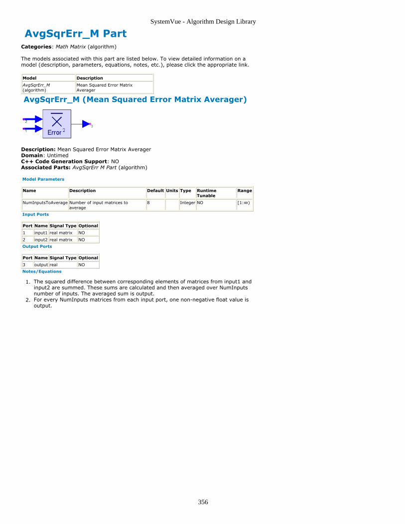
SystemVue - Algorithm Design Library
356
AvgSqrErr_M PartCategories: Math Matrix (algorithm)
The models associated with this part are listed below. To view detailed information on amodel (description, parameters, equations, notes, etc.), please click the appropriate link.
Model Description
AvgSqrErr_M(algorithm)
Mean Squared Error MatrixAverager
AvgSqrErr_M (Mean Squared Error Matrix Averager)
Description: Mean Squared Error Matrix AveragerDomain: UntimedC++ Code Generation Support: NOAssociated Parts: AvgSqrErr M Part (algorithm)
Model Parameters
Name Description Default Units Type RuntimeTunable
Range
NumInputsToAverage Number of input matrices toaverage
8 Integer NO [1:∞)
Input Ports
Port Name Signal Type Optional
1 input1 real matrix NO
2 input2 real matrix NO
Output Ports
Port Name Signal Type Optional
3 output real NO
Notes/Equations
The squared difference between corresponding elements of matrices from input1 and1.input2 are summed. These sums are calculated and then averaged over NumInputsnumber of inputs. The averaged sum is output.For every NumInputs matrices from each input port, one non-negative float value is2.output.

SystemVue - Algorithm Design Library
357
Conjugate_M PartCategories: Math Matrix (algorithm)
The models associated with this part are listed below. To view detailed information on amodel (description, parameters, equations, notes, etc.), please click the appropriate link.
Model Description
Conjugate_M(algorithm)
Conjugate MatrixFunction
Conjugate_M (Conjugate Matrix Function)
Description: Conjugate Matrix FunctionDomain: UntimedC++ Code Generation Support: NOAssociated Parts: Conjugate M Part (algorithm)
Input Ports
Port Name Signal Type Optional
1 input complex matrix NO
Output Ports
Port Name Signal Type Optional
2 output complex matrix NO
Notes/Equations
The input matrix is copied to output with each element replaced with the complex1.conjugate of that element.For every input matrix, an output matrix is written.2.

SystemVue - Algorithm Design Library
358
Gain PartCategories: C++ Code Generation (algorithm), Math Matrix (algorithm), Math Scalar(algorithm)
The models associated with this part are listed below. To view detailed information on amodel (description, parameters, equations, notes, etc.), please click the appropriate link.
Model Description
Gain (algorithm) Constant Gain
Amplifier (algorithm) Nonlinear Amplifier with Noise Figure
GainFxp (hardware) Fixed Point Gain
NegateFxp(hardware)
Fixed Point Negate

SystemVue - Algorithm Design Library
359
Gain
Description: Constant GainDomain: UntimedC++ Code Generation Support: YES (see Note)Associated Parts: Gain Part (algorithm)
Model Parameters
Name Description Default Units Type Runtime Tunable
Gain Gain value 1 None YES
Input Ports
Port Name Signal Type Optional
1 input anytype NO
Output Ports
Port Name Signal Type Optional
2 output anytype NO
NoteThis model does not support C++ code generation if the port type is resolved to envelope signal (sim),fixed point (sim), or variant (sim).
Notes/Equations
Gain multiplies the input by the Gain parameter.1.For every input, a product is output.2.As the Gain parameter is a variant, the product may be promoted from the input3.type, e.g. if the Gain parameter is a complex matrix while the input is real, theoutput will be a complex matrix. For discussion on the variant type, see Variant(sim).
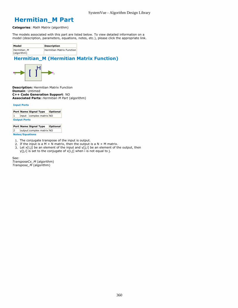
SystemVue - Algorithm Design Library
360
Hermitian_M PartCategories: Math Matrix (algorithm)
The models associated with this part are listed below. To view detailed information on amodel (description, parameters, equations, notes, etc.), please click the appropriate link.
Model Description
Hermitian_M(algorithm)
Hermitian Matrix Function
Hermitian_M (Hermitian Matrix Function)
Description: Hermitian Matrix FunctionDomain: UntimedC++ Code Generation Support: NOAssociated Parts: Hermitian M Part (algorithm)
Input Ports
Port Name Signal Type Optional
1 input complex matrix NO
Output Ports
Port Name Signal Type Optional
2 output complex matrix NO
Notes/Equations
The conjugate transpose of the input is output.1.If the input is a M × N matrix, then the output is a N × M matrix.2.Let x[i,j] be an element of the input and y[j,i] be an element of the output, then3.y[j,i] is set to the conjugate of x[i,j] when i is not equal to j.
See:TransposeCx_M (algorithm)Transpose_M (algorithm)

SystemVue - Algorithm Design Library
361
Identity_M PartCategories: Math Matrix (algorithm), Sources (algorithm)
The models associated with this part are listed below. To view detailed information on amodel (description, parameters, equations, notes, etc.), please click the appropriate link.
Model Description
Identity_M (algorithm) Identity Matrix Generator
IdentityCx_M(algorithm)
Complex Identity MatrixGenerator
Identity_M (Identity Matrix Generator)
Description: Identity Matrix GeneratorDomain: TimedC++ Code Generation Support: NOAssociated Parts: Identity M Part (algorithm)
Model Parameters
Name Description Default Units Type RuntimeTunable
Range Symbol
RowsCols Number of rows andcolumns in outputsquare matrix
2 Integer NO [2:∞) RC
ShowAdvancedParams Show advancedparameters: NO, YES
NO Enumeration NO
SampleRateOption Sample rate option:UnTimed, Timed fromSampleRate, Timedfrom Schematic
Timed fromSchematic
Enumeration NO SO
SampleRate Explicit sample rate Sample_Rate Hz Float NO ( 0:∞)
S
InitialDelay Output sample delay 0 Integer YES [ 0:∞)
D
Output Ports
Port Name Signal Type Optional
1 output real matrix NO
Notes/Equations
Identity_M is a constant square matrix source whose dimensions are specified by the1.RowsCols parameter.The constant matrix is formed by inserting real ones into the diagonal elements2.beginning at element [1,1]. Zeroes are inserted at the off diagonal elements.For other parameter descriptions, see Untimed Sources (algorithm).3.Fill value is a real matrix zero.4.
See:IdentityCx_M (algorithm)Diagonal_M (algorithm)DiagonalCx_M (algorithm)Const (algorithm)
IdentityCx_M (Complex Identity Matrix Generator)
Description: Complex Identity Matrix GeneratorDomain: TimedC++ Code Generation Support: NOAssociated Parts: Identity M Part (algorithm)
Model Parameters

SystemVue - Algorithm Design Library
362
Name Description Default Units Type RuntimeTunable
Range Symbol
RowsCols Number of rows andcolumns in outputsquare matrix
2 Integer NO [2:∞) RC
ShowAdvancedParams Show advancedparameters: NO, YES
NO Enumeration NO
SampleRateOption Sample rate option:UnTimed, Timed fromSampleRate, Timedfrom Schematic
Timed fromSchematic
Enumeration NO SO
SampleRate Explicit sample rate Sample_Rate Hz Float NO ( 0:∞)
S
InitialDelay Output sample delay 0 Integer YES [ 0:∞)
D
Output Ports
Port Name Signal Type Optional
1 output complex matrix NO
Notes/Equations
IdentityCx_M is a constant square matrix source whose dimensions are specified by1.the RowsCols parameter.The constant matrix is formed by inserting complex ones into the diagonal elements2.beginning at element [1,1]. Zeroes are inserted at the off diagonal elements.For other parameter descriptions, see Untimed Sources (algorithm).3.Fill value is a complex matrix zero.4.
See:Identity_M (algorithm)Diagonal_M (algorithm)DiagonalCx_M (algorithm)Const (algorithm)

SystemVue - Algorithm Design Library
363
Inverse_M PartCategories: Math Matrix (algorithm)
The models associated with this part are listed below. To view detailed information on amodel (description, parameters, equations, notes, etc.), please click the appropriate link.
Model Description
Inverse_M (algorithm) Inverse Matrix Function
InverseCx_M(algorithm)
Complex Inverse MatrixFunction
Inverse_M (Inverse Matrix Function)
Description: Inverse Matrix FunctionDomain: UntimedC++ Code Generation Support: NOAssociated Parts: Inverse M Part (algorithm)
Input Ports
Port Name Signal Type Optional
1 input real matrix NO
Output Ports
Port Name Signal Type Optional
2 output real matrix NO
Notes/Equations
The output matrix is the inverse of the input matrix, i.e.1.
For every input matrix, an inverse matrix is output.2.The input matrix must be square.3.
See:InverseCx_M (algorithm)
InverseCx_M (Complex Inverse Matrix Function)
Description: Complex Inverse Matrix FunctionDomain: UntimedC++ Code Generation Support: NOAssociated Parts: Inverse M Part (algorithm)
Input Ports
Port Name Signal Type Optional
1 input complex matrix NO
Output Ports
Port Name Signal Type Optional
2 output complex matrix NO
Notes/Equations
The output matrix is the inverse of the input matrix, i.e.1.
For every input matrix, an inverse matrix is output.2.The input matrix must be square.3.
See Inverse_M (algorithm).

SystemVue - Algorithm Design Library
364
Mapper_M PartCategories: C++ Code Generation (algorithm), Communications (algorithm), Math Matrix(algorithm)
The models associated with this part are listed below. To view detailed information on amodel (description, parameters, equations, notes, etc.), please click the appropriate link.
Model Description
Mapper_M(algorithm)
Most significant bit first. BPSK, QPSK, PSK8, QAM16, QAM32, QAM64, QAM128,QAM256
<#comment></#comment><#comment></#comment>
Mapper_M (Most significant bit first)
Description: Most significant bit first. BPSK, QPSK, PSK8, QAM16, QAM32, QAM64,QAM128, QAM256Domain: UntimedC++ Code Generation Support: YESAssociated Parts: Mapper M Part (algorithm)
Input Ports
Port Name Signal Type Optional
1 In boolean matrix NO
Output Ports
Port Name Signal Type Optional
2 Out complex NO
Notes/Equations
The Mapper_M model maps an input boolean matrix into a complex constellation1.point. The modulation type is dynamically determined by the number of elements inthe input matrix. The bits are grouped by reading the matrix in column-major order,with the first matrix element being interpreted as the most significant bit.A constellation point is a pair of real values (I,Q) that is expressed on the output as I2.+ jQ. Later in the modulation chain, I modulates the inphase part of the carrier, andQ modulates the quadrature part of the carrier over a symbol period.Each modulation type has its constellation and symbol length. The symbol length, i.e.3.the number of input bits per symbol, is detailed in the following table.
Modulation Type and Symbol Length
Symbol Length (Number of matrix elements) Modulation Type
1 BPSK
2 QPSK
3 PSK8
4 QAM16
5 QAM32
6 QAM64
7 QAM128
8 QAM256
For QPSK and PSK8 the mapping from bits to symbols is using Gray encoding. For1.QAM16, QAM32, QAM64, QAM128, and QAM256, Gray encoding is used inside eachquadrant.For BPSK, bit value 0 is mapped to 1 + j0 and bit value 1 is mapped to -1 + j0.2.For QPSK, the constellation map is illustrated in QPSK Constellation (algorithm). For3.PSK8, the constellation map is illustrated in 8PSK Constellation (algorithm).The symbol mappings for QAM16, QAM32, QAM64, QAM128 and QAM256 are4.described in the section 9 of [1], and their constellation maps are illustrated in figure7-8 of [1].QAM constellations need definition only for quadrant 1. The constellation points in5.quadrants 2, 3 and 4 are derived from quadrant 1 by selecting the quadrant 1constellation value with the least significant bits of the input symbol and rotating thatconstellation value by the amount selected by the two most significant bits of theinput symbol, b i b q, as specified in table Conversion of Constellation Points
(algorithm).

SystemVue - Algorithm Design Library
365
Conversion of Constellation Points
Quadrant Symbol Most Significant Bits ( b i b q ) Rotation
1 00 0
2 10 π/2
3 11 π
4 01 3π/2
16QAM, 32QAM, 64QAM, 128QAM and 256QAM constellation maps are illustrated in 16and 32QAM Constellation (algorithm) through 256QAM Constellation (algorithm).
SeeMapper (algorithm)Demapper (algorithm)
References
EN 300 429, "Digital Video Broadcasting (DVB); Framing structure, channel coding1.and modulation for cable systems," V1.2.1, 1998-04.
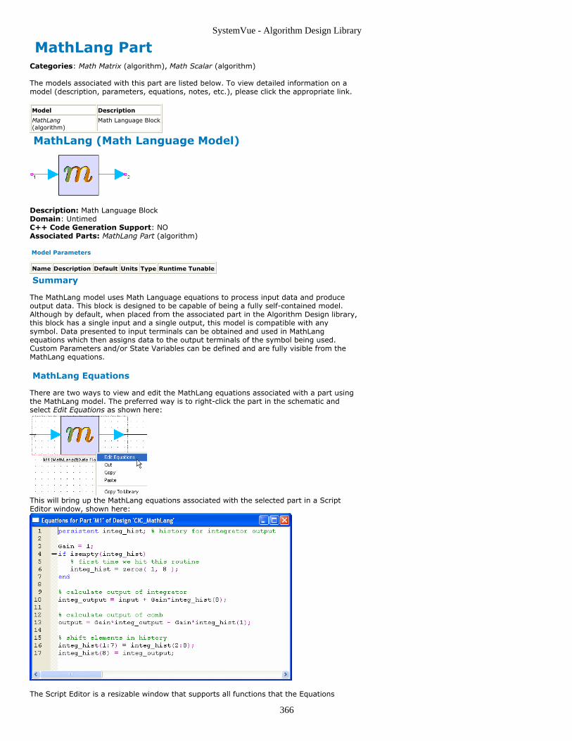
SystemVue - Algorithm Design Library
366
MathLang PartCategories: Math Matrix (algorithm), Math Scalar (algorithm)
The models associated with this part are listed below. To view detailed information on amodel (description, parameters, equations, notes, etc.), please click the appropriate link.
Model Description
MathLang(algorithm)
Math Language Block
MathLang (Math Language Model)
Description: Math Language BlockDomain: UntimedC++ Code Generation Support: NOAssociated Parts: MathLang Part (algorithm)
Model Parameters
Name Description Default Units Type Runtime Tunable
Summary
The MathLang model uses Math Language equations to process input data and produceoutput data. This block is designed to be capable of being a fully self-contained model.Although by default, when placed from the associated part in the Algorithm Design library,this block has a single input and a single output, this model is compatible with anysymbol. Data presented to input terminals can be obtained and used in MathLangequations which then assigns data to the output terminals of the symbol being used.Custom Parameters and/or State Variables can be defined and are fully visible from theMathLang equations.
MathLang Equations
There are two ways to view and edit the MathLang equations associated with a part usingthe MathLang model. The preferred way is to right-click the part in the schematic andselect Edit Equations as shown here:
This will bring up the MathLang equations associated with the selected part in a ScriptEditor window, shown here:
The Script Editor is a resizable window that supports all functions that the Equations

SystemVue - Algorithm Design Library
367
window supports, such as setting breakpoints, Find and Replace, etc. For details about theEquations window, see Equations (users).
Another way to view and edit the equations is to double-click on the part in the schematic.This will bring up the standard Part Parameters dialog box with a MathLang-specific userinterface. The first tab is labeled Equations and contains the editable equations.Setting/Removing breakpoints and performing Find and Replace operations is alsosupported in this Equations tab. The Equations tab looks like this:
Configuring Inputs and Outputs
The I/O tab, shown here, is used to configure the inputs and outputs used by theMathLang equations:
The first column, Symbol Port Name, displays the names of the ports of the currentsymbol assigned to the part. The current symbol can be seen in the upper-right handcorner of the Part Properties dialog box. The second column, Name in Equations,represents the name that the corresponding symbol port is refered to as in the MathLangequations. The Direction column specifies whether the corresponding symbol port is aninput or an output. The MultiPort column specifies whether the corresponding symbol portis a bus terminal or a single terminal. Note: Bus Terminals will produce a variable oftype Cell Array, in which each element of the Cell Array corresponds to a sub-terminal of the bus. Even if there is only one object connected to the bus, a cell array oflength 1 is produced. The index into the cell array corresponds to the ordering defined inthe Netlist of the part. Finally, the Port Rates column allows the user to set the Rate(s) ofthe port and is discussed in more detail in the Port Rates section below.
Examples referencing the above 'input' and 'output' equation names:When the 'input' has 'Multiport' checked, but 'output' does not, then reference 'input' inthe 'Equations' page using cell array notation: output = 12.5 * input { 4 }. The valueassigned to 'output' is 12.5 times the 4th member of the 'input' cell array.Similarly, when the 'output' has 'Multiport' checked, but 'input' does not, then reference'output' in the 'Equations' page using cell array notation: output { 4 } = 12.5 * input. Thevalue assigned to the 4th member of the 'output' cell array is 12.5 times the input.
Inputs and Outputs are added or removed by clicking the Add Port and Delete Portbuttons, respectively. Note that if the Symbol Port Name column has an empty entry, thatmeans the current symbol does not have a terminal to map to the port associated withthat row. In other words, the port defined by that row will not receive any data.
To load preconfigured I/O configurations, Inherit from Symbol and Inherit from Modelbuttons are provided. Since a Symbol contains no information about directionality of aterminal, or whether the terminal is a single-port or a bus, the Inherit from Symbol buttoncan only intelligently inherit symbol terminal names from a symbol. Models, on the otherhand, contain all information about their ports, so the Inherit from Model button allowsone to extract all I/O information from a model.

SystemVue - Algorithm Design Library
368
Custom Parameters and States
The Custom Parameters tab, shown here, allows you to define parameters or states thatare visible from within your MathLang equations:
The table seen in this tab allows you to set values for parameters that you haveconfigured. This table is identical to the usual Part Parameters entry table seen in mostparts. To define Parameters, use the Define Custom Parameters button. The resultingdialog box allows you to define parameters in a manner identical to the way one woulddefine Parameters for a Sub-Network model (ie. the Parameters tab of a Design). SeeCreating a Design with Parameters (users) for details on defining Parameters.
Port Rates
The rate of a port determines how many samples to collect (input rate), or how manysamples to generate (output rate), for each simulator clock tick.
For example, suppose we have a constant source feeding a MathLang block with the value1 on every clock tick. If we set the input Rates parameter to be 3, the simulator will waitto collect 3 samples before firing the MathLang block's equations. Therefore, for that clocktick, the MathLang block would see a vector [1; 1; 1] as the current sample, in effectdecreasing the sampling rate by a factor of 3.
Similarly, suppose that in our MathLang equations we assign a vector [1; 2; 3] to anoutput terminal which has an output Rate set to 3. The block would then output 3samples: 1, 2, and 3, in effect increasing the sampling rate by a factor of 3.
Suppose input port rate is R (larger than 1). If input samples are with the same scalartype, the MathLang block would see a R x 1 vector. If the input samples are matrices withthe same size M x N, the MathLang block would see a R x M x N structure. If inputsamples are in different dimensions or different sizes, the MathLang block would see a R x1 cell array.
For Bus ports, the corresponding Rates parameter can be a scalar, in which case it appliesthat rate to all sub-terminals for that port. It may also be a vector which defines a rate foreach sub-terminal separately.
How the Simulator invokes the MathLang Block
The simulator looks for 3 specific functions in the MathLang block to execute: Initialize,Run, and Finalize. Note: If no function definition is present in your MathLangequations (ie. you just have equation script commands), then your script iswrapped into the Run function automatically.
The Initialize function, if present, is called once at the begining of the simulation run. Itcan be used to pre-allocate data or perform any sort of initialization. The Finalize function,if present, is called once at the end of the simulation run and can be used to performclean-up.
The Run function is invoked by the simulator for every clock tick, ie. every time input ispresented to the block. Variables defined in the Run function do not persist between callsunless they are declared as persistent.
Differences Between MATLAB and MathLang Persistent Variables
There are a few big differences in how persistent variables are treated in MATLAB andMathLang:
The lifespan of a persistent variable in MATLAB is the entire MATLAB session nomatter how many SystemVue simulations are run. In addition, its scope is "global"meaning that there is only one persistent variable no matter how many parts makeuse of the MATLAB code defining the persistent variable.

SystemVue - Algorithm Design Library
369
The lifespan of a persistent variable in MathLang is the duration of the simulation it isused in. In addition, its scope is "local" meaning that each part making use of theMathLang code defining the persistent variable has its own instance of the persistentvariable.
Here is an example that will help clarify the above. Assume the following code is used tocreate a compiled M code model (see README.txt file in <SystemVue InstallationDirectory>\ModelBuilder\SystemVue Compiled M Code Models)
function [ out ] = MyFFE( Coefficients, SamplesPerBit, in )
persistent dSamples;
persistent numSamples;
persistent taps;
if isempty(dSamples)
% first time we hit this routine
numSamples = length(Coefficients) * SamplesPerBit;
dSamples = zeros( 1, numSamples);
dSamples(1) = in;
taps = Coefficients';
else
dSamples = [in,dSamples(1:numSamples-1)];
end
out = dSamples(1:SamplesPerBit:numSamples) * taps;
end
There are several issues with the use of this code in a SystemVue simulation:
Having more than one instance of a part using this code will produce wrong1.simulation results. The reason is that the parts will share the same set of persistentvariables and will corrupt each other's state.Even a single instance of a part using this code is problematic if more than one2.simulation is run. The reason is that the persistent variables are initialized only once(at the beginning of the first simulation that made use of this code). After that,dSamples will never be empty again so the block of code that initializes the persistentvariables will never be triggered again. The result is that at the beginning of eachsimulation the first few output samples will be incorrect (until the dSamples bufferfills with data from the current simulation). In addition, if the Coefficients andSamplesPerBit are defined as parameters of the compiled M code SystemVue model,changing their values on the schematic will not have any effect on the simulationresults since again the code that initializes them is not going to be trigerred after thefirst simulation is run.
The exact same code (without the first "function" line and the last "end" line) used in aMathLang part does not suffer from either of the two issues mentioned above. See theMyFFE.m MATLAB code in <SystemVue Installation Directory>\ModelBuilder\SystemVueCompiled M Code Models directrory for an example on how to write the MATLAB code in away that does not suffer from the second problem described above. This requires that theSystemVue model wrapper code is also written in a special way to make sure the MATLABpersistent variables are initialized at the beginning of every simulation. There is no way toavoid the first problem described above.
Examples
Suppose we wanted to define an Adder with a Gain parameter. First, we define configurethe inputs and outputs. We define one input named "input" and check the MultiPortcolumn since we want the adder to add an arbitrary number of inputs. We define a singleoutput named "output" which we leave as a single-port, since the adder produces only oneresult.
In the Custom Parameters tab, we click the Define Custom Parameters button and definea single parameter called Gain.
The MathLang code which sums all of the inputs, scales by the Gain parameter, andproduces an output might look like this:
nInputs = numel( input );
sum = 0;
for i = 1 : nInputs
sum = sum + input{i}; % input is a cell array
end
output = Gain * sum; % Gain was defined in Custom Parameters tab
Here's a more complex example that uses a persistent variable named State to retainstate in between calls:
persistent State;
% initialize the structure on the first tic
if isempty( State ) % is it the first call?
State.Amount = 1
State.Clock = 0
State.Flag= 1 % increase so we don't call this block again

SystemVue - Algorithm Design Library
370
end
% increment to the next clock tic
State.Clock = State.Clock+1
%
% at each 100 clocks bump the amount
if ( State.Clock == 100)
State.Amount = State.Amount * 1.1
State.Clock = 0; % reset clock
end
% now scale the input data
if input >= 1
output = State.Amount * sqrt( input )
else
output = input
end
Finally, if we wanted to define Initialize and Finalize functions, we could do as follows:
function Initialize()
% Set up code and pre-allocation goes here
function Run()
% compute outputs based on inputs
function Finalize()
% Clean up code goes here

SystemVue - Algorithm Design Library
371
MATLAB_Cosim PartCategories: Math Matrix (algorithm)
The models associated with this part are listed below. To view detailed information on amodel (description, parameters, equations, notes, etc.), please click the appropriate link.
Model Description
MATLAB_Cosim(algorithm)
MATLAB Cosimulation Block
MATLAB_Cosim (MATLAB Cosimulation Block)
Description: MATLAB Cosimulation BlockDomain: UntimedC++ Code Generation Support: NOAssociated Parts: MATLAB Cosim Part (algorithm)
Model Parameters
Name Description Default Units Type RuntimeTunable
ScriptDirectory Optional directory for location of custom Matlab files Text NO
MatlabSetUp Matlab command to execute during begin method Text NO
MatlabFunction Matlab command to execute for each simulationsample
Text NO
MatlabWrapUp Matlab command to execute during wrapup method Text NO
Input Ports
Port Name Signal Type Optional
1 input multiplevariant
YES
Output Ports
Port Name Signal Type Optional
2 output multiple complex matrix NO
Notes/Equations
See MATLAB Cosimulation (sim) for detailed information about MATLAB_Cosim.1.

SystemVue - Algorithm Design Library
372
Mpy PartCategories: C++ Code Generation (algorithm), Math Matrix (algorithm), Math Scalar(algorithm)
The models associated with this part are listed below. To view detailed information on amodel (description, parameters, equations, notes, etc.), please click the appropriate link.
Model Description
Mpy (algorithm) Multiple Input Multiplier
MpyMultiEnv(algorithm)
Multiple Input EnvelopeMultiplier
MpyFxp (hardware) Fixed Point Multiplier
Mpy(Multiple Input Multiplier)
Description: Multiple Input MultiplierDomain: UntimedC++ Code Generation Support: YES (see Note)Associated Parts: Mpy Part (algorithm)
Input Ports
Port Name Signal Type Optional
1 input multiple anytype NO
Output Ports
Port Name Signal Type Optional
2 output anytype NO
NoteThis model does not support C++ code generation if the port type is resolved to envelope signal (sim),fixed point (sim), or variant (sim).
Notes/Equations
Mpy outputs the product of the inputs.1.This model reads 1 sample from all inputs and writes 1 sample to the output.2.For a single input multiply, the input is copied to the output.3.

SystemVue - Algorithm Design Library
373
MpyMultiEnv (Multiple Input EnvelopeMultiplier)
Description: Multiple Input Envelope MultiplierDomain: TimedC++ Code Generation Support: NOAssociated Parts: Mpy Part (algorithm)
Model Parameters
Name Description Default Units Type RuntimeTunable
SideBandType Multiplication product type: Lower sideband,Upper sideband, Both sidebands
Uppersideband
Enumeration NO
Input Ports
Port Name Description Signal Type Optional
1 input input signal multipleenvelope
NO
Output Ports
Port Name Description Signal Type Optional
2 output output signal envelope NO
Notes/Equations
This model implements a multiple input envelope multiplier.1.When the number of inputs is 2, then this model performs exactly the same as the2.two input envelope multiplier MpyEnv (algorithm).When the number of inputs is greater than 2, then the only SideBandType supported3.is Upper sideband. In this case, this model acts as a cascade of MpyEnv (algorithm)models, that is, the first two input envelope signals are multiplied using the two inputMpyEnv (algorithm) model, the resulting signal is multiplied with the third inputenvelope signal using another two input MpyEnv (algorithm) model, the resultingsignal is is multiplied with the fourth input envelope signal using another two inputMpyEnv (algorithm) model, etc.
See:AddEnv (algorithm)SubEnv (algorithm)MpyEnv (algorithm)
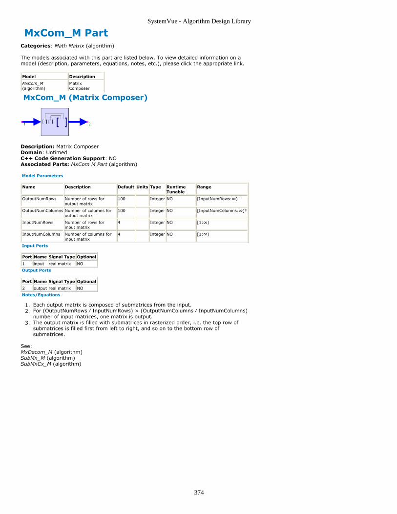
SystemVue - Algorithm Design Library
374
MxCom_M PartCategories: Math Matrix (algorithm)
The models associated with this part are listed below. To view detailed information on amodel (description, parameters, equations, notes, etc.), please click the appropriate link.
Model Description
MxCom_M(algorithm)
MatrixComposer
MxCom_M (Matrix Composer)
Description: Matrix ComposerDomain: UntimedC++ Code Generation Support: NOAssociated Parts: MxCom M Part (algorithm)
Model Parameters
Name Description Default Units Type RuntimeTunable
Range
OutputNumRows Number of rows foroutput matrix
100 Integer NO [InputNumRows:∞)†
OutputNumColumns Number of columns foroutput matrix
100 Integer NO [InputNumColumns:∞)‡
InputNumRows Number of rows forinput matrix
4 Integer NO [1:∞)
InputNumColumns Number of columns forinput matrix
4 Integer NO [1:∞)
Input Ports
Port Name Signal Type Optional
1 input real matrix NO
Output Ports
Port Name Signal Type Optional
2 output real matrix NO
Notes/Equations
Each output matrix is composed of submatrices from the input.1.For (OutputNumRows ⁄ InputNumRows) × (OutputNumColumns ⁄ InputNumColumns)2.number of input matrices, one matrix is output.The output matrix is filled with submatrices in rasterized order, i.e. the top row of3.submatrices is filled first from left to right, and so on to the bottom row ofsubmatrices.
See:MxDecom_M (algorithm)SubMx_M (algorithm)SubMxCx_M (algorithm)

SystemVue - Algorithm Design Library
375
MxDecom_M PartCategories: Math Matrix (algorithm)
The models associated with this part are listed below. To view detailed information on amodel (description, parameters, equations, notes, etc.), please click the appropriate link.
Model Description
MxDecom_M(algorithm)
Matrix Decomposer
MxDecom_M (Matrix Decomposer)
Description: Matrix DecomposerDomain: UntimedC++ Code Generation Support: NOAssociated Parts: MxDecom M Part (algorithm)
Model Parameters
Name Description Default Units Type RuntimeTunable
Range
StartRow Starting row in input matrix togenerate output matrices (firstrow is 1)
1 Integer NO [1:∞)
StartCol Starting column in input matrixto generate output matrices(first column is 1, matrix upperleft corner is (1,1)
1 Integer NO [1:∞)
InputNumRows Number of rows for input matrix 100 Integer NO [OutputNumRows:∞)†
InputNumCols Number of columns from inputmatrix
100 Integer NO [OutputNumCols:∞)‡
OutputNumRows Number of rows for outputmatrix
4 Integer NO [1:∞)
OutputNumCols Number of columns for outputmatrix
4 Integer NO [1:∞)
Input Ports
Port Name Description Signal Type Optional
1 input Input matrix to be decomposed into the outputsubmatrices.
real matrix NO
Output Ports
Port Name Description Signal Type Optional
2 output Output matrices with dimensionsOutputNumRows*OutputNumCols.
real matrix NO
Notes/Equations
Each output matrix is a nonoverlapping submatrix of the input.1.For every input matrix, (OutputNumRows ⁄ InputNumRows) × (OutputNumColumns ⁄2.InputNumColumns) number of matrices are output.The output matrices are extracted from the input in rasterized order, i.e. the top row3.of submatrices is retrieved first from left to right, and so on to the bottom row ofsubmatrices.
See:MxCom_M (algorithm)SubMx_M (algorithm)SubMxCx_M (algorithm)

SystemVue - Algorithm Design Library
376
Pack_M PartCategories: C++ Code Generation (algorithm), Math Matrix (algorithm), Type Converters(algorithm)
The models associated with this part are listed below. To view detailed information on amodel (description, parameters, equations, notes, etc.), please click the appropriate link.
Model Description
Pack_M(algorithm)
Pack Matrix Function
Pack_M (Pack Matrix Function)
Description: Pack Matrix FunctionDomain: UntimedC++ Code Generation Support: YES (see Note)Associated Parts: Pack M Part (algorithm)
Model Parameters
Name Description Default Units Type RuntimeTunable
Range
NumRows Number of rows in output matrix 1 Integer NO [1:∞)
NumCols Number of columns in output matrix 1 Integer NO [1:∞)
Format Format of data to be packed into matrix:ColumnMajor, RowMajor
ColumnMajor Enumeration NO
Input Ports
Port Name Signal Type Optional
1 input anytype NO
Output Ports
Port Name Signal Type Optional
2 output anytype matrix NO
NoteThis model does not support C++ code generation if the port type is resolved to envelope signal (sim) orvariant (sim).
Notes/Equations
The Pack_M model packs NumRows x NumCols input scalar values into an output1.matrix with NumRows and NumCols.This model reads NumRows x NumCols scalar samples from the input and writes one2.matrix to the output with NumRows and NumCols.Inputs are entered into the matrix output in either column-major or row-major order3.based using the Format parameter.
See:Unpack_M (algorithm)DynamicPack_M (algorithm)DynamicUnpack_M (algorithm)

SystemVue - Algorithm Design Library
377
SampleMean_M PartCategories: Math Matrix (algorithm)
The models associated with this part are listed below. To view detailed information on amodel (description, parameters, equations, notes, etc.), please click the appropriate link.
Model Description
SampleMean_M(algorithm)
Matrix MeanValue
SampleMean_M (Matrix Mean Value)
Description: Matrix Mean ValueDomain: UntimedC++ Code Generation Support: NOAssociated Parts: SampleMean M Part (algorithm)
Input Ports
Port Name Signal Type Optional
1 input real matrix NO
Output Ports
Port Name Signal Type Optional
2 output real NO
Notes/Equations
The averaged value of all elements of the input matrix is output.1.For input matrix, one real value is output.2.

SystemVue - Algorithm Design Library
378
SubMx_M PartCategories: Math Matrix (algorithm)
The models associated with this part are listed below. To view detailed information on amodel (description, parameters, equations, notes, etc.), please click the appropriate link.
Model Description
SubMx_M (algorithm) Submatrix Extractor
SubMxCx_M(algorithm)
Complex Submatrix Extractor
SubMx_M (Submatrix Extractor)
Description: Submatrix ExtractorDomain: UntimedC++ Code Generation Support: NOAssociated Parts: SubMx M Part (algorithm)
Model Parameters
Name Description Default Units Type RuntimeTunable
Range
StartRow Starting row for the submatrix within the inputmatrix
1 Integer NO [1:∞)
StartCol Starting column for the submatrix within theinput matrix
1 Integer NO [1:∞)
NumRows Number of submatrix rows 2 Integer NO [1:∞)
NumCols Number of submatrix columns 2 Integer NO [1:∞)
Input Ports
Port Name Signal Type Optional
1 input real matrix NO
Output Ports
Port Name Signal Type Optional
2 output real matrix NO
Notes/Equations
Output a submatrix of the input.1.For every input matrix, a submatrix is output.2.The parameters specify the dimensions of the output and the upper left position3.within the input where extraction begins.
See:SubMxCx_M (algorithm)MxDecom_M (algorithm)MxCom_M (algorithm)
SubMxCx_M (Complex Submatrix Extractor)
Description: Complex Submatrix ExtractorDomain: UntimedC++ Code Generation Support: NOAssociated Parts: SubMx M Part (algorithm)
Model Parameters

SystemVue - Algorithm Design Library
379
Name Description Default Units Type RuntimeTunable
Range
StartRow Starting row for the submatrix within the inputmatrix
1 Integer NO [1:∞)
StartCol Starting column for the submatrix within theinput matrix
1 Integer NO [1:∞)
NumRows Number of submatrix rows 1 Integer NO [1:∞)
NumCols Number of submatrix columns 1 Integer NO [1:∞)
Input Ports
Port Name Signal Type Optional
1 input complex matrix NO
Output Ports
Port Name Signal Type Optional
2 output complex matrix NO
Notes/Equations
Output a submatrix of the input.1.For every input matrix, a submatrix is output.2.The parameters specify the dimensions of the output and the upper left position3.within the input where extraction begins.
See:SubMx_M (algorithm)MxDecom_M (algorithm)MxCom_M (algorithm)
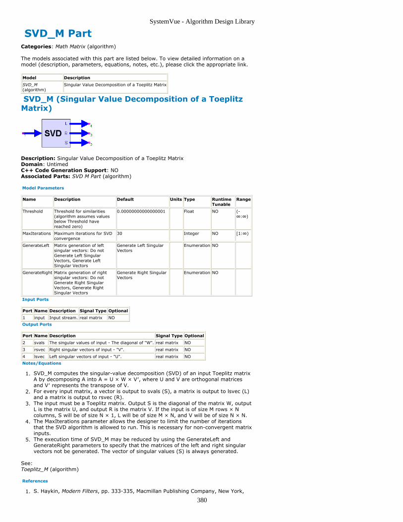
SystemVue - Algorithm Design Library
380
SVD_M PartCategories: Math Matrix (algorithm)
The models associated with this part are listed below. To view detailed information on amodel (description, parameters, equations, notes, etc.), please click the appropriate link.
Model Description
SVD_M(algorithm)
Singular Value Decomposition of a Toeplitz Matrix
SVD_M (Singular Value Decomposition of a ToeplitzMatrix)
Description: Singular Value Decomposition of a Toeplitz MatrixDomain: UntimedC++ Code Generation Support: NOAssociated Parts: SVD M Part (algorithm)
Model Parameters
Name Description Default Units Type RuntimeTunable
Range
Threshold Threshold for similarities(algorithm assumes valuesbelow Threshold havereached zero)
0.00000000000000001 Float NO (-∞:∞)
MaxIterations Maximum iterations for SVDconvergence
30 Integer NO [1:∞)
GenerateLeft Matrix generation of leftsingular vectors: Do notGenerate Left SingularVectors, Generate LeftSingular Vectors
Generate Left SingularVectors
Enumeration NO
GenerateRight Matrix generation of rightsingular vectors: Do notGenerate Right SingularVectors, Generate RightSingular Vectors
Generate Right SingularVectors
Enumeration NO
Input Ports
Port Name Description Signal Type Optional
1 input Input stream. real matrix NO
Output Ports
Port Name Description Signal Type Optional
2 svals The singular values of input - The diagonal of "W". real matrix NO
3 rsvec Right singular vectors of input - "V". real matrix NO
4 lsvec Left singular vectors of input - "U". real matrix NO
Notes/Equations
SVD_M computes the singular-value decomposition (SVD) of an input Toeplitz matrix1.A by decomposing A into A = U × W × V′, where U and V are orthogonal matricesand V′ represents the transpose of V.For every input matrix, a vector is output to svals (S), a matrix is output to lsvec (L)2.and a matrix is output to rsvec (R).The input must be a Toeplitz matrix. Output S is the diagonal of the matrix W, output3.L is the matrix U, and output R is the matrix V. If the input is of size M rows × Ncolumns, S will be of size N × 1, L will be of size M × N, and V will be of size N × N.The MaxIterations parameter allows the designer to limit the number of iterations4.that the SVD algorithm is allowed to run. This is necessary for non-convergent matrixinputs.The execution time of SVD_M may be reduced by using the GenerateLeft and5.GenerateRight parameters to specify that the matrices of the left and right singularvectors not be generated. The vector of singular values (S) is always generated.
See:Toeplitz_M (algorithm)
References
S. Haykin, Modern Filters, pp. 333-335, Macmillan Publishing Company, New York,1.

SystemVue - Algorithm Design Library
381
1989.

SystemVue - Algorithm Design Library
382
Toeplitz_M PartCategories: Math Matrix (algorithm)
The models associated with this part are listed below. To view detailed information on amodel (description, parameters, equations, notes, etc.), please click the appropriate link.
Model Description
Toeplitz_M (algorithm) Toeplitz Matrix Converter
ToeplitzCx_M(algorithm)
Complex Toeplitz Matrix Converter
Toeplitz_M (Toeplitz Matrix Converter)
Description: Toeplitz Matrix ConverterDomain: UntimedC++ Code Generation Support: NOAssociated Parts: Toeplitz M Part (algorithm)
Model Parameters
Name Description Default Units Type Runtime Tunable Range
NumRows Number of rows in the output matrix 2 Integer NO [1:∞)
NumCols Number of columns in the outputmatrix
2 Integer NO [1:∞)
Input Ports
Port Name Description Signal Type Optional
1 input Input stream. real NO
Output Ports
Port Name Description Signal Type Optional
2 output the data matrixX.
real matrix NO
Notes/Equations
The Toeplitz_M model packs NumRows + NumCols − 1 input real scalar values into1.an output real matrix with NumRows and NumCols.This model reads NumRows + NumCols − 1 real scalar samples from the input and2.writes 1 real matrix (X) to the output with NumRows and NumCols.Let M = NumCols, N = NumRows + NumCols − 1 and x[1:N] be the input, then from3.left to right:The first (top) row of X is x[M] x[M−1]) ... x[1],the second row of X is x[M + 1] x[M] ... x[2],untilthe last (bottom) row of X, which is x[N] x[N − 1] ... x[N − M + 1]. Note that N = M+ NumRows − 1 and N − M + 1 = NumRows.
See:ToeplitzCx_M (algorithm)Identity_M (algorithm)IdentityCx_M (algorithm)Diagonal_M (algorithm)DiagonalCx_M (algorithm)Const (algorithm)
ToeplitzCx_M (Complex Toeplitz Matrix Converter)
Description: Complex Toeplitz Matrix ConverterDomain: UntimedC++ Code Generation Support: NOAssociated Parts: Toeplitz M Part (algorithm)
Model Parameters

SystemVue - Algorithm Design Library
383
Name Description Default Units Type Runtime Tunable Range
NumRows Number of rows in the output matrix 2 Integer NO [1:∞)
NumCols Number of columns in the outputmatrix
2 Integer NO [1:∞)
Input Ports
Port Name Description Signal Type Optional
1 input Input stream. complex NO
Output Ports
Port Name Description Signal Type Optional
2 output Data matrixX.
complex matrix NO
Notes/Equations
The ToeplitzCx_M model packs NumRows + NumCols − 1 input complex scalar values1.into an output complex matrix with NumRows and NumCols.This model reads NumRows + NumCols − 1 complex scalar samples from the input2.and writes 1 complex matrix (X) to the output with NumRows and NumCols.Let M = NumCols, N = NumRows + NumCols − 1 and x[1:N] be the input, then from3.left to right:The first (top) row of X is x[M] x[M − 1]) ... x[1],the second row of X is x[M + 1] x[M] ... x[2],untilthe last (bottom) row of X, which is x[N] x[N − 1] ... x[N − M + 1]. Note that N = M+ NumRows − 1 and N − M + 1 = NumRows.
See:Toeplitz_M (algorithm)Identity_M (algorithm)IdentityCx_M (algorithm)Diagonal_M (algorithm)DiagonalCx_M (algorithm)Const (algorithm)

SystemVue - Algorithm Design Library
384
Transpose_M PartCategories: Math Matrix (algorithm)
The models associated with this part are listed below. To view detailed information on amodel (description, parameters, equations, notes, etc.), please click the appropriate link.
Model Description
Transpose_M (algorithm) Matrix Transposer
TransposeCx_M(algorithm)
Complex MatrixTransposer
Transpose_M (Matrix Transposer)
Description: Matrix TransposerDomain: UntimedC++ Code Generation Support: NOAssociated Parts: Transpose M Part (algorithm)
Input Ports
Port Name Signal Type Optional
1 input real matrix NO
Output Ports
Port Name Signal Type Optional
2 output real matrix NO
Notes/Equations
The transpose of the input is output.1.If the input is a M × N matrix, then the output is a N × M matrix.2.Let x[i,j] be an element of the input and y[j,i] be an element of the output, then3.y[j,i] = x[i,j].
See:TransposeCx_M (algorithm)Hermitian_M (algorithm)
TransposeCx_M (Complex Matrix Transposer)
Description: Complex Matrix TransposerDomain: UntimedC++ Code Generation Support: NOAssociated Parts: Transpose M Part (algorithm)
Input Ports
Port Name Signal Type Optional
1 input complex matrix NO
Output Ports
Port Name Signal Type Optional
2 output complex matrix NO
Notes/Equations
The transpose of the input is output.1.If the input is a M × N matrix, then the output is a N × M matrix.2.Let x[i,j] be an element of the input and y[j,i] be an element of the output, then3.y[j,i] = x[i,j].
See:Transpose_M (algorithm)Hermitian_M (algorithm)

SystemVue - Algorithm Design Library
385
Unpack_M PartCategories: C++ Code Generation (algorithm), Math Matrix (algorithm), Type Converters(algorithm)
The models associated with this part are listed below. To view detailed information on amodel (description, parameters, equations, notes, etc.), please click the appropriate link.
Model Description
Unpack_M(algorithm)
Unpack Matrix Function
Unpack_M (Unpack Matrix Function)
Description: Unpack Matrix FunctionDomain: UntimedC++ Code Generation Support: YES (see Note)Associated Parts: Unpack M Part (algorithm)
Model Parameters
Name Description Default Units Type RuntimeTunable
Range
NumRows Number of rows in input matrix 1 Integer NO [1:∞)
NumCols Number of columns in input matrix 1 Integer NO [1:∞)
Format Format of data to be packed into matrix:ColumnMajor, RowMajor
ColumnMajor Enumeration NO
Input Ports
Port Name Signal Type Optional
1 input anytype matrix NO
Output Ports
Port Name Signal Type Optional
2 output anytype NO
NoteThis model does not support C++ code generation if the port type is resolved to envelope signal (sim) orvariant (sim).
Notes/Equations
The Unpack_M model unpacks an input matrix to write NumRows x NumCols values1.to the output. If the matrix is too small, zero-padding will be used for the missingelements. If the matrix is too larger, the extra elements will be ignored.This model reads one matrix from the input and writes NumRows x NumCols scalar2.samples to the output.Elements of the input matrix of dimension, NumRow × NumCols, are output in either3.column-major or row-major order based using the Format parameter.
See:Pack_M (algorithm)DynamicPack_M (algorithm)DynamicUnpack_M (algorithm)

SystemVue - Algorithm Design Library
386
BitShiftRegister PartCategories: Math Scalar (algorithm)
The models associated with this part are listed below. To view detailed information on amodel (description, parameters, equations, notes, etc.), please click the appropriate link.
Model Description
BitShiftRegister(algorithm)
Bit ShiftRegister

SystemVue - Algorithm Design Library
387
BitShiftRegister
Description: Bit Shift RegisterDomain: UntimedC++ Code Generation Support: NOAssociated Parts: BitShiftRegister Part (algorithm)
Model Parameters
Name Description Default Units Type Runtime Tunable Range
NumBits Number of bits in the outputregister
8 Integer NO [1:∞)
BitOrder Output bit order: LSB first, MSB first MSBfirst
Enumeration YES
Input Ports
Port Name Description Signal Type Optional
1 input input bits boolean NO
2 clock clock int YES
3 reset reset int YES
Output Ports
Port Name Description Signal Type Optional
4 output output bitregister
boolean NO
Notes/Equations
The BitShiftRegister model reads input bit values and writes to the output the current1.and NumBits-1 prior bits in a shift register stream with LSB or MSB first based onBitOrder and dependent on the state of the reset and clock inputs.This model reads 1 sample from the inputs (input , clock , reset ) and writes NumBits2.samples to the output. The clock and reset inputs are optional.When the clock is not connected, it is set internally to one.3.When the reset is not connected, it is set internally to zero.4.When reset is one (regardless of the clock ), then all NumBits samples written to the5.output are set to zero.When clock is one, then the current input bit is read and is loaded into and shifts all6.prior bits in the output register.The output resigter is sent out with either LSB (least significant bit) or MSB (most7.significant bit) ordering based on the setting of BitOrder .To select only the 'n'th output bit, one can follow this part with a DownSample part8.with Factor set to NumBits and Phase set to 'n'.

SystemVue - Algorithm Design Library
388
BitsToInt PartCategories: C++ Code Generation (algorithm), Math Scalar (algorithm), Type Converters(algorithm)
The models associated with this part are listed below. To view detailed information on amodel (description, parameters, equations, notes, etc.), please click the appropriate link.
Model Description
BitsToInt(algorithm)
Bits to Integer Converter
BitsToInt(Bits to Integer Converter)
Description: Bits to Integer ConverterDomain: UntimedC++ Code Generation Support: YESAssociated Parts: BitsToInt Part (algorithm)
Model Parameters
Name Description Default Units Type Runtime Tunable
NumBits Number of bits read per execution 4 Integer NO
BitOrder Bit order: LSB first, MSB first MSBfirst
Enumeration YES
Input Ports
Port Name Signal Type Optional
1 input boolean NO
Output Ports
Port Name Signal Type Optional
2 output int NO
Notes/Equations
The BitsToInt model converts NumBits successive input bit values, packs these bits1.into an integer, and outputs the integer.This model reads NumBits samples from the input and interprets it using the BitOrder2.parameter to write 1 sample to the output.When the input is any nonzero value, a one bit value is input, otherwise a zero bit is3.input.The BitOrder parameter determines how successive inputs bits are packed into the4.integer. If BitOrder is specified as LSB first, then the first input bit becomes the leastsignificant bit of the output, i.e. controls whether the output is even or odd.Otherwise, the last input bit becomes the least significant bit of the output.If NumBits is greater than the number of bits forming an integer, the most significant5.bits are lost.If NumBits is greater than or equal to the number of bits forming an integer, the6.output could be negative. Otherwise, the output is always nonnegative.When symbols are mapped onto an integer, this part becomes a BitToSymbol7.converter.
See:IntToBits (algorithm)

SystemVue - Algorithm Design Library
389
CxToPolar PartCategories: Math Scalar (algorithm), Type Converters (algorithm)
The models associated with this part are listed below. To view detailed information on amodel (description, parameters, equations, notes, etc.), please click the appropriate link.
Model Description
CxToPolar(algorithm)
Complex to Magnitude and Phase Converter
CxToPolar (Complex to Magnitude and PhaseConverter)
Description: Complex to Magnitude and Phase ConverterDomain: UntimedC++ Code Generation Support: NOAssociated Parts: CxToPolar Part (algorithm)
Input Ports
Port Name Signal Type Optional
1 input complex NO
Output Ports
Port Name Signal Type Optional
2 magnitude real NO
3 phase real NO
Notes/Equations
The CxToPolar model converts input complex values to output magnitude and angle1.values.This model reads 1 sample from the input and writes 1 sample to each of the outputs2.magnitude and phase.magnitude = | input |phase = input (the phase is in radians)
See:unwrap (algorithm)CxToRect (algorithm)PolarToCx (algorithm)RectToCx (algorithm)

SystemVue - Algorithm Design Library
390
CxToRect PartCategories: C++ Code Generation (algorithm), Math Scalar (algorithm), Type Converters(algorithm)
The models associated with this part are listed below. To view detailed information on amodel (description, parameters, equations, notes, etc.), please click the appropriate link.
Model Description
CxToRect(algorithm)
double CxToRect
CxToRect (Complex to Real and ImaginaryConverter)
Description: double CxToRectDomain: UntimedC++ Code Generation Support: YESAssociated Parts: CxToRect Part (algorithm)
Input Ports
Port Name Signal Type Optional
1 input complex NO
Output Ports
Port Name Signal Type Optional
2 real real NO
3 imag real NO
Notes/Equations
The CxToRect model converts input complex values to output real and imaginary1.values.This model reads 1 sample from the input and writes 1 sample to each of the outputs2.real and imag.real = real partimag = imaginary part
See:CxToPolar (algorithm)RectToCx (algorithm)PolarToCx (algorithm)

SystemVue - Algorithm Design Library
391
DB PartCategories: Math Scalar (algorithm)
The models associated with this part are listed below. To view detailed information on amodel (description, parameters, equations, notes, etc.), please click the appropriate link.
Model Description
db(algorithm)
Decibel Function
db
Description: Decibel FunctionDomain: UntimedC++ Code Generation Support: NOAssociated Parts: DB Part (algorithm)
Model Parameters
Name Description Default Units Type RuntimeTunable
Range
Min Minimum output value -100 Float YES (-∞:∞)
DbType Type of dB value: Power as10*log(input), Amplitude as20*log(input)
Amplitude as20*log(input)
Enumeration YES
Input Ports
Port Name Signal Type Optional
1 input real NO
Output Ports
Port Name Signal Type Optional
2 output real NO
Notes/Equations
DB converts the input to a decibel (dB) scale. Zero and negative inputs convert to the1.Min value.If the input is a power measurement set DbType to Power as 10log(input), else the2.input is an amplitude measurement so set DbType to Power as 20log(input).If Power as 10log(input):3.
If Power as 20log(input):
where:x(n) is input for sample ny(n) is output for sample n

SystemVue - Algorithm Design Library
392
Dirichlet PartCategories: Math Scalar (algorithm)
The models associated with this part are listed below. To view detailed information on amodel (description, parameters, equations, notes, etc.), please click the appropriate link.
Model Description
Dirichlet(algorithm)
Dirichlet (Aliased Sinc)Function
Dirichlet (Dirichlet (Aliased Sinc) Function)
Description: Dirichlet (Aliased Sinc) FunctionDomain: UntimedC++ Code Generation Support: NOAssociated Parts: Dirichlet Part (algorithm)
Model Parameters
Name Description Default Units Type Runtime Tunable Range
N Length of Dirichlet kernel 10 Integer YES [1:∞)
Input Ports
Port Name Description Signal Type Optional
1 input input to the Dirichlet kernel real NO
Output Ports
Port Name Description Signal Type Optional
2 output output of the Dirichlet kernel real NO
Notes/Equations
Dirichlet computes the normalized Dirichlet kernel (also called the aliased sinc1.function).The value of the normalized Dirichlet kernel at x = 0 is always 1, and the normalized2.Dirichlet kernel oscillates between −1 and +1. The normalized Dirichlet kernel isperiodic in x with a period of either 2π when N is odd or 4π when N is even.The Dirichlet kernel is the discrete-time Fourier transform (DTFT) of a sampled pulse3.function. The parameter N is the length of the pulse [1].
See:sinc (algorithm).
References
A. V. Oppenheim and R. W. Schafer, Discrete-Time Signal Processing, Prentice-Hall:1.Englewood Cliffs, NJ, 1989.

SystemVue - Algorithm Design Library
393
Integrator PartCategories: Math Scalar (algorithm)
The models associated with this part are listed below. To view detailed information on amodel (description, parameters, equations, notes, etc.), please click the appropriate link.
Model Description
Integrator (algorithm) Integrator with Reset
IntegratorCx (algorithm) Complex integrator withReset
IntegratorInt(algorithm)
Integer Integrator with Reset
Integrator (Integrator with Reset)
Description: Integrator with ResetDomain: TimedC++ Code Generation Support: NOAssociated Parts: Integrator Part (algorithm)
Model Parameters
Name Description Default Units Type RuntimeTunable
Range
IntegrationMethod Integration method: Rectangle,Trapezoidal
Rectangle Enumeration YES
LimitOutput Output limiter options: No,Saturate, Wrap
No Enumeration YES
Top Upper limit. Visible whenLimitOutput is enabled.
0 Float YES (-∞:∞)
Bottom Lower limit. Visible whenLimitOutput is enabled.
0 Float YES (-∞:∞)
InitialState Initial integrator state 0 Float NO (-∞:∞)
UseIntegrationWindow Enable integration window: No,DefinedInTime, DefinedInSamples
No Enumeration NO
FeedbackGain Gain on feedback path. Visiblewhen UseIntegrationWindow isdisabled.
1 Float YES (-∞:∞)
IntegrationTime Integration time. Visible whenUseIntegrationWindow isDefinedInTime.
100e-6 s Float NO (0:∞)
IntegrationSamples Integration samples. Visible whenUseIntegrationWindow isDefinedInSamples.
100 Integer NO [2:∞)
Input Ports
Port Name Description Signal Type Optional
1 reset reset int YES
2 data input real NO
Output Ports
Port Name Description Signal Type Optional
3 output output real NO
Notes/Equations
The input port is numerically integrated in a method chosen by the1.IntegrationMethod parameter. The integration value is output.For every input, there is one output.2.If the reset input is non-zero (true), the integration value is set to the current input.3.To enable a continuous accumulation, leave the reset port unconnected or connect azero Const source to the reset port.Limits to the output are controlled by the LimitOutput parameter. If LimitOutput is No4., no limiting is performed, otherwise the output is kept between Top and Bottom.If LimitOutput is Saturate then the integration value is clamped between Top and5.Bottom, otherwise wrap around is performed.The InitialState value is applied only to the first output.6.

SystemVue - Algorithm Design Library
394
If UseIntegrationWindow is either DefineInTime or DefineInSamples, the integration7.is performed over the most recent window of samples. Samples before the first arezero valued.When UseIntegrationWindow is No, leakage can be modeled by the FeedbackGain8.parameter. The output is the input plus the product of FeedbackGain and theprevious integration value.With the default parameters, input values are accumulated and the accumulation is9.output.
See:IntegratorCx (algorithm)IntegratorInt (algorithm)SlidWinAvg (algorithm)

SystemVue - Algorithm Design Library
395
IntegratorCx
Description: Complex integrator with ResetDomain: TimedC++ Code Generation Support: NOAssociated Parts: Integrator Part (algorithm)
Model Parameters
Name Description Default Units Type RuntimeTunable
Range
IntegrationMethod Integration method: Rectangle,Trapezoidal
Rectangle Enumeration YES
LimitOutput Output limiter options: No,Saturate, Wrap
No Enumeration YES
Top Upper magnitude limit. Visiblewhen LimitOutput is enabled.
0 Float YES (-∞:∞)
Bottom Lower magnitude limit. Visiblewhen LimitOutput is enabled.
0 Float YES (-∞:∞)
InitialState Initial integrator state 0 Complexnumber
NO (-∞:∞)
UseIntegrationWindow Enable integration window: No,DefinedInTime, DefinedInSamples
No Enumeration NO
FeedbackGain Gain on feedback path 1 Float YES (-∞:∞)
IntegrationTime Integration time. Visible whenUseIntegrationWindow isDefinedInTime.
100e-6 s Float NO (0:∞)
IntegrationSamples Integration samples. Visible whenUseIntegrationWindow isDefinedInSamples.
100 Integer NO [2:∞)
Input Ports
Port Name Description Signal Type Optional
1 reset reset int YES
2 data input complex NO
Output Ports
Port Name Description Signal Type Optional
3 output output complex NO
Notes/Equations
The input port is numerically integrated in a method chosen by the1.IntegrationMethod parameter. The integration value is output.For every input, there is one output.2.If the reset input is non-zero (true), the integration value is set to the current input.3.To enable a continuous accumulation, leave the reset port unconnected or connect azero Const source to the reset port.Limits to the output are controlled by the LimitOutput parameter. If LimitOutput is No4., no limiting is performed, otherwise the output magnitude is kept between Top andBottom.If LimitOutput is Saturate then the magnitude of the integration value is clamped5.between Top and Bottom, otherwise wrap around is performed.The InitialState value is applied only to the first output.6.If UseIntegrationWindow is either DefineInTime or DefineInSamples, the integration7.is performed over the most recent window of samples. Samples before the first arezero valued.When UseIntegrationWindow is No, leakage can be modeled by the FeedbackGain8.parameter. The output is the input plus the product of FeedbackGain and theprevious integration value.With the default parameters, input values are accumulated and the accumulation is9.output.
See also: Integrator (algorithm), IntegratorInt (algorithm), SlidWinAvg (algorithm).

SystemVue - Algorithm Design Library
396
IntegratorInt
Description: Integer Integrator with ResetDomain: TimedC++ Code Generation Support: NOAssociated Parts: Integrator Part (algorithm)
Model Parameters
Name Description Default Units Type RuntimeTunable
Range
LimitOutput Output limiter options: No, Saturate,Wrap
No Enumeration YES
Top Upper integer limit. Visible whenLimitOutput is enabled.
0 Integer YES (-∞:∞)
Bottom Lower integer limit. Visible whenLimitOutput is enabled.
0 Integer YES (-∞:∞)
InitialState Initial integrator state 0 Integer NO (-∞:∞)
UseIntegrationWindow Enable integration window: No,DefinedInTime, DefinedInSamples
No Enumeration NO
IntegrationTime Integration time. Visible whenUseIntegrationWindow isDefinedInTime.
100e-6 s Float NO (0:∞)
IntegrationSamples Integration samples. Visible whenUseIntegrationWindow isDefinedInSamples.
100 Integer NO [2:∞)
Input Ports
Port Name Description Signal Type Optional
1 reset reset int YES
2 data input int NO
Output Ports
Port Name Description Signal Type Optional
3 output output int NO
Notes/Equations
Input is summed and output.1.For every input, there is one output.2.If the reset input is non-zero (true), the sum is set to the current input. To enable a3.continuous accumulation, leave the reset port unconnected or connect a zero Constsource to the reset port.Limits to the output are controlled by the LimitOutput parameter. If LimitOutput is No4., no limiting is performed, otherwise the output is kept between Top and Bottom.If LimitOutput is Saturate then the sum is clamped between Top and Bottom,5.otherwise wrap around is performed.The InitialState value is applied only to the first output.6.If UseIntegrationWindow is either DefineInTime or DefineInSamples, the integration7.is performed over the most recent window of samples. Samples before the first arezero valued.With the default parameters, input values are accumulated and the accumulation is8.output.
See also: Integrator (algorithm), IntegratorCx (algorithm), SlidWinAvg (algorithm).

SystemVue - Algorithm Design Library
397
IntToBits PartCategories: C++ Code Generation (algorithm), Math Scalar (algorithm), Type Converters(algorithm)
The models associated with this part are listed below. To view detailed information on amodel (description, parameters, equations, notes, etc.), please click the appropriate link.
Model Description
IntToBits(algorithm)
Integer to Bits Converter
IntToBits (Integer to Bits Converter)
Description: Integer to Bits ConverterDomain: UntimedC++ Code Generation Support: YESAssociated Parts: IntToBits Part (algorithm)
Model Parameters
Name Description Default Units Type Runtime Tunable
NumBits Number of output bits per input sample 4 Integer NO
BitOrder Bit order: LSB first, MSB first MSBfirst
Enumeration YES
Input Ports
Port Name Signal Type Optional
1 input int NO
Output Ports
Port Name Signal Type Optional
2 output boolean NO
Notes/Equations
The IntToBits model extracts the least significant NumBits number of bits from an1.integer input and serial outputs the bits as zeros and ones.This model reads 1 sample from the input and interprets it using the BitOrder2.parameter to write NumBits samples to the output.If BitOrder is specified as LSB first, then the least significant bit is output first. If3.nBits is greater than the number of bits forming an integer, the most significant bitsabove the number of bits forming an integer are lost and are assigned the input signbit, i.e. a one bit if the input is negative.When symbols are mapped onto an integer, this part becomes a SymbolToBits4.converter.To select only the 'n'th output bit, one can follow this part with a DownSample part5.with Factor set to NumBits and Phase set to 'n'.
See:BitsToInt (algorithm)

SystemVue - Algorithm Design Library
398
Logic PartCategories: C++ Code Generation (algorithm), Math Scalar (algorithm)
The models associated with this part are listed below. To view detailed information on amodel (description, parameters, equations, notes, etc.), please click the appropriate link.
Model Description
Logic (algorithm) Boolean Logic Function
AND_Fxp (hardware) Fixed Point Bitwise AND
NAND_Fxp(hardware)
Fixed Point Bitwise NAND
NOR_Fxp (hardware) Fixed Point Bitwise NOR
NOT_Fxp (hardware) Fixed Point NOT
OR_Fxp (hardware) Fixed Point Bitwise OR
XNOR_Fxp (hardware) Fixed Point Bitwise XNOR
XOR_Fxp (hardware) Fixed Point Bitwise XOR
Logic (Boolean Logic Function)
Description: Boolean Logic FunctionDomain: UntimedC++ Code Generation Support: YESAssociated Parts: Logic Part (algorithm)
Model Parameters
Name Description Default Units Type RuntimeTunable
Logic Logic operation: NOT, AND, NAND, OR, NOR, XOR,XNOR
AND Enumeration NO
Input Ports
Port Name Description Signal Type Optional
1 input Input logicvalues.
multiple boolean NO
Output Ports
Port Name Description SignalType
Optional
2 output Result of the logic test, with FALSE equal to zero and TRUE equal to anon-zero integer (not necessarily 1).
boolean NO
Notes/Equations
A logical operation selected by the Logic parameter is applied to the inputs. The NOT1.operation can have only one input.The inputs are interpreted as booleans, i.e. false when the input is zero, otherwise2.true.This part's symbol text changes when the "Logic" parameter value is changed. That is3."AND", "OR", "XOR", etc. is based on the value of the "Logic" parameter. This isaccomplished via a %ParameterName% macro (in the annotation text), a featurewhich is end-user accessable. See Symbols (users) for more info.

SystemVue - Algorithm Design Library
399
MathCx PartCategories: Math Scalar (algorithm)
The models associated with this part are listed below. To view detailed information on amodel (description, parameters, equations, notes, etc.), please click the appropriate link.
Model Description
MathCx(algorithm)
Complex Math Function
MathCx (Complex Math Function)
Description: Complex Math FunctionDomain: UntimedC++ Code Generation Support: YESAssociated Parts: Math Part (algorithm)
Model Parameters
Name Description Default Units Type RuntimeTunable
FunctionType Mathematical function: Abs, Ceil, Exp, Floor, Ln,Log10, Pow10, Recip, Round, Sqr, Sqrt, Conj
Abs Enumeration NO
Input Ports
Port Name Signal Type Optional
1 input complex NO
Output Ports
Port Name Signal Type Optional
2 output complex NO
Notes/Equations
Math calculates complex mathematical functions:1.y(n) = f(x(n))where:f( ) is a function selected by the FunctionType parameterx(n) is input for sample ny(n) is output for sample nIf the function cannot be calculated, the simulation is halted with an error message.2.For FunctionType:3.
Abs, y(n) = |x(n)| =
Ceil, y(n) = See Ceil function of Math component.
Exp, y(n) = e x(n) = e Re{x(n)} (cos(Im{x(n)}) + j sin(Im{x(n)}))
Floor, y(n) = See Floor function of Math component.
Ln, y(n) = , where is the phase of x(n)in radians.Log10, y(n) = log 10 (x(n)) = ln(x(n)) / ln(10)
Pow10, y(n) = 10 x(n) = e x(n) ln(10)
Recip, y(n) = 1 / x(n) = (Re{x(n)} − j Im{x(n)}) / |x(n)| 2
Round, y(n) = Round(Re{x(n)}) + j Round(Im{x(n)})See Round function of Math component.
Sqr, y(n) = x(n) 2
Sqrt, y(n) = , where is the phase ofx(n) in radians.
Conj, y(n) =
See:Math (algorithm)Trig (algorithm)TrigCx (algorithm)

SystemVue - Algorithm Design Library
400
Math PartCategories: C++ Code Generation (algorithm), Math Scalar (algorithm)
The models associated with this part are listed below. To view detailed information on amodel (description, parameters, equations, notes, etc.), please click the appropriate link.
Model Description
Math (algorithm) Math Function
MathCx (algorithm) Complex Math Function
ABS_Fxp(hardware)
Fixed Point Absolute Value
SqrtFxp (hardware) Fixed Point Square Root
Math (Math Function)
Description: Math FunctionDomain: UntimedC++ Code Generation Support: YESAssociated Parts: Math Part (algorithm)
Model Parameters
Name Description Default Units Type RuntimeTunable
FunctionType Mathematical function: Abs, Ceil, Exp, Floor, Ln,Log10, Pow10, Recip, Round, Sqr, Sqrt, Sgn
Abs Enumeration NO
Input Ports
Port Name Signal Type Optional
1 input real NO
Output Ports
Port Name Signal Type Optional
2 output real NO
Notes/Equations
Math calculates real mathematical functions:1.y(n) = f(x(n))where:f( ) is a function selected by the FunctionTypex(n) is input for sample ny(n) is output for sample nIf the function cannot be calculated, the simulation is halted with an error message.2.For FunctionType:3.
Abs, y(n) = |x(n)|
Ceil, y(n) = , where Exp, y(n) = e x(n)
Floor, y(n) = , where Ln, y(n) = ln(x(n))Log10, y(n) = log 10 (x(n))
Pow10, y(n) = 10 x(n)
Recip, y(n) = 1 / x(n)Round, y(n) = closest integer to x(n)
When x(n) is at the same distance between integers, Round maps awayfrom 0, e.g. 2.5 maps to 3 and −2.5 maps to −3.
Sqr, y(n) = x(n) 2
Sqrt, y(n) = Sgn, y(n) = a number indicating the sign of the input n i.e., y(n) = 1 if n > 0;y(n) = 0 if n == 0; and y(n) = -1 if n < 0.
See:MathCx (algorithm)Trig (algorithm)TrigCx (algorithm)

SystemVue - Algorithm Design Library
401
Modulo PartCategories: Math Scalar (algorithm)
The models associated with this part are listed below. To view detailed information on amodel (description, parameters, equations, notes, etc.), please click the appropriate link.
Model Description
Modulo (algorithm) Modulo Function
ModuloInt(algorithm)
Integer Modulo Function
Modulo (Modulo Function)
Description: Modulo FunctionDomain: UntimedC++ Code Generation Support: NOAssociated Parts: Modulo Part (algorithm)
Model Parameters
Name Description Default Units Type Runtime Tunable Range
Modulo Modulo value 1 Float YES (-∞:0) or (0:∞)
Input Ports
Port Name Description Signal Type Optional
1 input input signal real NO
Output Ports
Port Name Description Signal Type Optional
2 output output signal real NO
Notes/Equations
Modulo outputs the remainder with the same sign as input after dividing the input by1.the Modulo parameter.
where:x(n) is input for sample ny(n) is output for sample nFor every input, there is an output.2.
See:ModuloInt (algorithm)

SystemVue - Algorithm Design Library
402
ModuloInt
Description: Integer Modulo FunctionDomain: UntimedC++ Code Generation Support: NOAssociated Parts: Modulo Part (algorithm)
Model Parameters
Name Description Default Units Type Runtime Tunable Range
Modulo Integer modulo value 8 Integer YES (0:∞)
Input Ports
Port Name Description Signal Type Optional
1 input input signal int NO
Output Ports
Port Name Description Signal Type Optional
2 output output signal int NO
Notes/Equations
ModuloInt functions identically to Modulo (algorithm) except that the operation is1.over integers.
See:Modulo (algorithm)

SystemVue - Algorithm Design Library
403
PolarToCx PartCategories: Math Scalar (algorithm), Type Converters (algorithm)
The models associated with this part are listed below. To view detailed information on amodel (description, parameters, equations, notes, etc.), please click the appropriate link.
Model Description
PolarToCx(algorithm)
Magnitude and Phase to Complex Converter
PolarToCx (Magnitude and Phase to ComplexConverter)
Description: Magnitude and Phase to Complex ConverterDomain: UntimedC++ Code Generation Support: NOAssociated Parts: PolarToCx Part (algorithm)
Input Ports
Port Name Signal Type Optional
1 magnitude real NO
2 phase real NO
Output Ports
Port Name Signal Type Optional
3 output complex NO
Notes/Equations
The PolarToCx model converts input magnitude and angle values to output complex1.values.output = magnitude × ( cos( phase ) + j × sin( phase ) )This model reads 1 sample from the inputs magnitude and phase and writes 12.sample to the output.The phase angle is specified in radians.3.
See:PolarToRect (algorithm)CxToPolar (algorithm)RectToPolar (algorithm)

SystemVue - Algorithm Design Library
404
PolarToRect PartCategories: Math Scalar (algorithm), Type Converters (algorithm)
The models associated with this part are listed below. To view detailed information on amodel (description, parameters, equations, notes, etc.), please click the appropriate link.
Model Description
PolarToRect(algorithm)
Magnitude and Phase to Rectangular Converter
PolarToRect (Magnitude and Phase to RectangularConverter)
Description: Magnitude and Phase to Rectangular ConverterDomain: UntimedC++ Code Generation Support: NOAssociated Parts: PolarToRect Part (algorithm)
Input Ports
Port Name Signal Type Optional
1 magnitude real NO
2 phase real NO
Output Ports
Port Name Signal Type Optional
3 x real NO
4 y real NO
Notes/Equations
The PolarToCx model converts input magnitude and phase values to output complex1.values.
x = magnitude * cos( phase )y = magnitude * sin( phase )
This model reads 1 sample from the inputs magnitude and phase and writes 12.sample to the outputs x and y.The phase is specified in radians.3.
See:PolarToCx (algorithm)RectToPolar (algorithm)CxToPolar (algorithm)

SystemVue - Algorithm Design Library
405
Polynomial PartCategories: Math Scalar (algorithm)
The models associated with this part are listed below. To view detailed information on amodel (description, parameters, equations, notes, etc.), please click the appropriate link.
Model Description
Polynomial (algorithm) Polynomial Mapper
PolynomialInt(algorithm)
Integer PolynomialMapper
Polynomial (Polynomial Mapper)
Description: Polynomial MapperDomain: UntimedC++ Code Generation Support: NOAssociated Parts: Polynomial Part (algorithm)
Model Parameters
Name Description Default Units Type RuntimeTunable
Coefficients Polynomial coefficients (0-th ordercoefficient first)
[0, 1] Floating pointarray
NO
Input Ports
Port Name Description Signal Type Optional
1 input input signal real NO
Output Ports
Port Name Description Signal Type Optional
2 output output signal real NO
Notes/Equations
Polynomial models a system with a polynomial input-output relationship.1.For every input, there is an output.2.If the input is x, the output is y = c 0 + c 1 × x + c 2 × x 2 + ... + c N × x N, where N3.is the order of the polynomial and c 0 , ... , c N are the elements of the Coefficients
parameter.
See:PolynomialInt (algorithm)

SystemVue - Algorithm Design Library
406
PolynomialInt
Description: Integer Polynomial MapperDomain: UntimedC++ Code Generation Support: NOAssociated Parts: Polynomial Part (algorithm)
Model Parameters
Name Description Default Units Type RuntimeTunable
Coefficients Integer polynomial coefficients (0-th ordercoefficient first)
[0, 1] Integerarray
NO
Input Ports
Port Name Description Signal Type Optional
1 input input signal int NO
Output Ports
Port Name Description Signal Type Optional
2 output output signal int NO
Notes/Equations
PolynomialInt functions identically to Polynomial (algorithm) except that the1.operation is over integers.
See:Polynomial (algorithm)

SystemVue - Algorithm Design Library
407
Reciprocal PartCategories: Math Scalar (algorithm)
The models associated with this part are listed below. To view detailed information on amodel (description, parameters, equations, notes, etc.), please click the appropriate link.
Model Description
Reciprocal(algorithm)
ReciprocalFunction
Reciprocal (Reciprocal Function)
Description: Reciprocal FunctionDomain: UntimedC++ Code Generation Support: NOAssociated Parts: Reciprocal Part (algorithm)
Model Parameters
Name Description Default Units Type RuntimeTunable
Range
MagLimit Magnitude limit; non-zero value limits the outputmagnitude
0 Float YES (-∞:∞)
Input Ports
Port Name Signal Type Optional
1 input real NO
Output Ports
Port Name Signal Type Optional
2 output real NO
Notes/Equations
The reciprocal of the input is calculated with an optional magnitude limit.1.If MagLimit = 0
If MagLimit ≠ 0 and input = 0y(n) = MagLimitIf MagLimit ≠ 0 and input ≠ 0
where:x(n) is input for sample ny(n) is output for sample n
See:Math (algorithm)MathCx (algorithm)

SystemVue - Algorithm Design Library
408
RectToCx PartCategories: C++ Code Generation (algorithm), Math Scalar (algorithm), Type Converters(algorithm)
The models associated with this part are listed below. To view detailed information on amodel (description, parameters, equations, notes, etc.), please click the appropriate link.
Model Description
RectToCx(algorithm)
double RectToCx
RectToCx (Real and Imaginary to ComplexConverter)
Description: double RectToCxDomain: UntimedC++ Code Generation Support: YESAssociated Parts: RectToCx Part (algorithm)
Input Ports
Port Name Signal Type Optional
1 real real YES
2 imag real YES
Output Ports
Port Name Signal Type Optional
3 output complex NO
Notes/Equations
The RectToCx model converts input real and imaginary values to output complex1.values.
output = real + j × imaginaryThis model reads 1 sample from the inputs real and imaginary and writes 1 sample to2.the output.
See:RectToPolar (algorithm)CxToRect (algorithm)PolarToRect (algorithm)

SystemVue - Algorithm Design Library
409
RectToPolar PartCategories: Math Scalar (algorithm), Type Converters (algorithm)
The models associated with this part are listed below. To view detailed information on amodel (description, parameters, equations, notes, etc.), please click the appropriate link.
Model Description
RectToPolar(algorithm)
Rectangular to PolarConverter
RectToPolar (Rectangular to Polar Converter)
Description: Rectangular to Polar ConverterDomain: UntimedC++ Code Generation Support: NOAssociated Parts: RectToPolar Part (algorithm)
Input Ports
Port Name Signal Type Optional
1 x real NO
2 y real NO
Output Ports
Port Name Signal Type Optional
3 magnitude real NO
4 phase real NO
Notes/Equations
The RectToPolar model converts input real and imaginary values to output magnitude1.and phase values.
magnitude = sqrt( real^2 + imaginary^2 )phase = atan2( imaginary, real )
This model reads 1 sample from the inputs real and imaginary and writes 1 sample to2.the outputs magnitude and phase.The phase angle is in the range -π to π radians.3.
See:RectToCx (algorithm)PolarToRect (algorithm)CxToRect (algorithm)
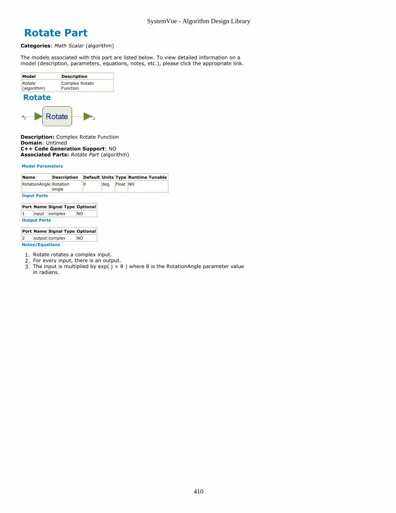
SystemVue - Algorithm Design Library
410
Rotate PartCategories: Math Scalar (algorithm)
The models associated with this part are listed below. To view detailed information on amodel (description, parameters, equations, notes, etc.), please click the appropriate link.
Model Description
Rotate(algorithm)
Complex RotateFunction
Rotate
Description: Complex Rotate FunctionDomain: UntimedC++ Code Generation Support: NOAssociated Parts: Rotate Part (algorithm)
Model Parameters
Name Description Default Units Type Runtime Tunable
RotationAngle Rotationangle
0 deg Float NO
Input Ports
Port Name Signal Type Optional
1 input complex NO
Output Ports
Port Name Signal Type Optional
2 output complex NO
Notes/Equations
Rotate rotates a complex input.1.For every input, there is an output.2.The input is multiplied by exp( j × θ ) where θ is the RotationAngle parameter value3.in radians.

SystemVue - Algorithm Design Library
411
Sinc PartCategories: Math Scalar (algorithm)
The models associated with this part are listed below. To view detailed information on amodel (description, parameters, equations, notes, etc.), please click the appropriate link.
Model Description
sinc(algorithm)
Sinc Function
sinc
Description: Sinc FunctionDomain: UntimedC++ Code Generation Support: NOAssociated Parts: Sinc Part (algorithm)
Input Ports
Port Name Description Signal Type Optional
1 input The input x to the sincfunction.
real NO
Output Ports
Port Name Description Signal Type Optional
2 output The output of the sinc function. real NO
Notes/Equations
The sinc function is defined as sin(x)/x which is continuous with value 1.0 when x =1.0. Input is in radians.For every input, there is an output.2.
See:Dirichlet (algorithm)

SystemVue - Algorithm Design Library
412
Sub PartCategories: C++ Code Generation (algorithm), Math Matrix (algorithm), Math Scalar(algorithm)
The models associated with this part are listed below. To view detailed information on amodel (description, parameters, equations, notes, etc.), please click the appropriate link.
Model Description
Sub (algorithm) Multiple Input Subtractor
SubEnv(algorithm)
Multiple Input Subtractor
SubFxp (hardware) Fixed Point Subtractor
Sub (Multiple Input Subtractor)
Description: Multiple Input SubtractorDomain: UntimedC++ Code Generation Support: YES (see Note)Associated Parts: Sub Part (algorithm)
Input Ports
Port Name Signal Type Optional
1 pos anytype NO
2 neg multiple anytype NO
Output Ports
Port Name Signal Type Optional
3 output anytype NO
NoteThis model does not support C++ code generation if the port type is resolved to envelope signal (sim),fixed point (sim), or variant (sim).
Notes/Equations
The Sub model subtracts all inputs at the neg input from the input at the pos input1.and produces the result at the output.This model reads 1 sample from all inputs and writes 1 sample to the output.2.For discussion on the variant type, see Variant (sim).3.

SystemVue - Algorithm Design Library
413
SubEnv (Multiple Input Subtractor)
Description: Multiple Input SubtractorDomain: TimedC++ Code Generation Support: NOAssociated Parts: Sub Part (algorithm)
Model Parameters
Name Description Default Units Type RuntimeTunable
Range Symbol
OutputFc Output characterization frequencyfor the combined signal: Min, Max,Center, User defined
Center Enumeration NO O
UserDefinedFc User defined outputcharacterization frequency
100e6 Hz Float NO [0:∞)† F
Input Ports
Port Name Description Signal Type Optional
1 pos envelope NO
2 neg input signals multipleenvelope
NO
Output Ports
Port Name Description Signal Type Optional
3 output output signal envelope NO
Notes/Equations
The SubEnv model subtracts all envelope signals connected to the neg port from the1.envelope signal connected to the pos port.This model reads 1 sample from all inputs and writes 1 sample to the output.2.For more information see the documentation of the AddEnv (algorithm) model.3.
See:AddEnv (algorithm)MpyEnv (algorithm)MpyMultiEnv (algorithm)
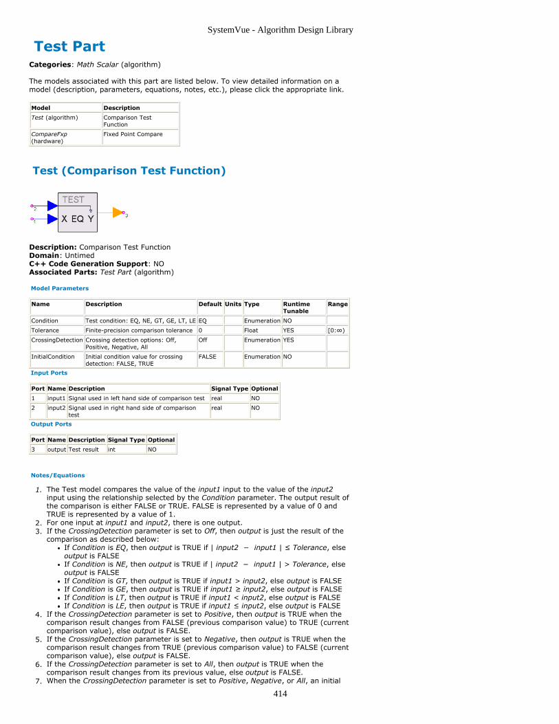
SystemVue - Algorithm Design Library
414
Test PartCategories: Math Scalar (algorithm)
The models associated with this part are listed below. To view detailed information on amodel (description, parameters, equations, notes, etc.), please click the appropriate link.
Model Description
Test (algorithm) Comparison TestFunction
CompareFxp(hardware)
Fixed Point Compare
Test (Comparison Test Function)
Description: Comparison Test FunctionDomain: UntimedC++ Code Generation Support: NOAssociated Parts: Test Part (algorithm)
Model Parameters
Name Description Default Units Type RuntimeTunable
Range
Condition Test condition: EQ, NE, GT, GE, LT, LE EQ Enumeration NO
Tolerance Finite-precision comparison tolerance 0 Float YES [0:∞)
CrossingDetection Crossing detection options: Off,Positive, Negative, All
Off Enumeration YES
InitialCondition Initial condition value for crossingdetection: FALSE, TRUE
FALSE Enumeration NO
Input Ports
Port Name Description Signal Type Optional
1 input1 Signal used in left hand side of comparison test real NO
2 input2 Signal used in right hand side of comparisontest
real NO
Output Ports
Port Name Description Signal Type Optional
3 output Test result int NO
Notes/Equations
The Test model compares the value of the input1 input to the value of the input21.input using the relationship selected by the Condition parameter. The output result ofthe comparison is either FALSE or TRUE. FALSE is represented by a value of 0 andTRUE is represented by a value of 1.For one input at input1 and input2, there is one output.2.If the CrossingDetection parameter is set to Off, then output is just the result of the3.comparison as described below:
If Condition is EQ, then output is TRUE if | input2 − input1 | ≤ Tolerance, elseoutput is FALSEIf Condition is NE, then output is TRUE if | input2 − input1 | > Tolerance, elseoutput is FALSEIf Condition is GT, then output is TRUE if input1 > input2, else output is FALSEIf Condition is GE, then output is TRUE if input1 ≥ input2, else output is FALSEIf Condition is LT, then output is TRUE if input1 < input2, else output is FALSEIf Condition is LE, then output is TRUE if input1 ≤ input2, else output is FALSE
If the CrossingDetection parameter is set to Positive, then output is TRUE when the4.comparison result changes from FALSE (previous comparison value) to TRUE (currentcomparison value), else output is FALSE.If the CrossingDetection parameter is set to Negative, then output is TRUE when the5.comparison result changes from TRUE (previous comparison value) to FALSE (currentcomparison value), else output is FALSE.If the CrossingDetection parameter is set to All, then output is TRUE when the6.comparison result changes from its previous value, else output is FALSE.When the CrossingDetection parameter is set to Positive, Negative, or All, an initial7.

SystemVue - Algorithm Design Library
415
value is needed to compare the result of the first comparison against. This value isset in the InitialCondition parameter.

SystemVue - Algorithm Design Library
416
Trig PartCategories: C++ Code Generation (algorithm), Math Scalar (algorithm)
The models associated with this part are listed below. To view detailed information on amodel (description, parameters, equations, notes, etc.), please click the appropriate link.
Model Description
Trig (algorithm) Trigonometric Function
TrigCx(algorithm)
Complex TrigonometricFunction
Trig (Trigonometric Function)
Description: Trigonometric FunctionDomain: UntimedC++ Code Generation Support: YESAssociated Parts: Trig Part (algorithm)
Model Parameters
Name Description Default Units Type RuntimeTunable
FunctionType Trigonometric function type: Sin, Cos, Tan, Cot,Asin, Acos, Atan, Acot, Sinh, Cosh, Tanh, Coth,Asinh, Acosh, Atanh, Acoth
Sin Enumeration NO
Input Ports
Port Name Signal Type Optional
1 input real NO
Output Ports
Port Name Signal Type Optional
2 output real NO
Notes/Equations
Trig calculates real trigonometric functions:1.y(n) = f(x(n))where:f( ) is a function selected by the Type parameterx(n) is input for sample ny(n) is output for sample nIf the function cannot be calculated, the simulation is halted with an error message.2.All angles are in radians.3.
See:TrigCx (algorithm)Math (algorithm)MathCx (algorithm)
TrigCx (Complex Trigonometric Function)
Description: Complex Trigonometric FunctionDomain: UntimedC++ Code Generation Support: YESAssociated Parts: Trig Part (algorithm)
Model Parameters

SystemVue - Algorithm Design Library
417
Name Description Default Units Type RuntimeTunable
FunctionType Complex trigonometric function type: Sin, Cos, Tan,Cot, Asin, Acos, Atan, Acot, Sinh, Cosh, Tanh, Coth,Asinh, Acosh, Atanh, Acoth
Sin Enumeration NO
Input Ports
Port Name Signal Type Optional
1 input complex NO
Output Ports
Port Name Signal Type Optional
2 output complex NO
Notes/Equations
TrigCx calculates complex trigonometric functions:1.y(n) = f(x(n))where:f( ) is a function selected by the Type parameterx(n) is input for sample ny(n) is output for sample nThe principal value is calculated.2.If the function cannot be calculated, the simulation is halted with an error message.3.All angles are in radians.4.
See:Trig (algorithm)Math (algorithm)MathCx (algorithm)
References
Handbook of Mathematical Functions, 1972, Abramowitz and Stegun.1.

SystemVue - Algorithm Design Library
418
Unwrap PartCategories: Math Scalar (algorithm)
The models associated with this part are listed below. To view detailed information on amodel (description, parameters, equations, notes, etc.), please click the appropriate link.
Model Description
unwrap(algorithm)
UnwrapPhase
unwrap
Description: Unwrap PhaseDomain: UntimedC++ Code Generation Support: NOAssociated Parts: Unwrap Part (algorithm)
Model Parameters
Name Description Default Units Type RuntimeTunable
Range
OutPhase Initial output phase 0 deg Float YES (-∞:∞)
PrevPhase Initial wrapped phase of input signal forcomputing the first phase difference
0 deg Float YES (-∞:∞)
PhaseType Phase type for the input and output signals:radians, degrees
radians Enumeration YES
Input Ports
Port Name Signal Type Optional
1 input real NO
Output Ports
Port Name Signal Type Optional
2 output real NO
Notes/Equations
Unwrap a phase plot by removing discontinuities of magnitude 2 π.1.For every input, there is an output.2.The phase is assumed to never change by more than π between inputs. The input is3.assumed to be in the range [−π, π].

SystemVue - Algorithm Design Library
419
Interpolator PartCategories: C++ Code Generation (algorithm), OFDM (algorithm)
The models associated with this part are listed below. To view detailed information on amodel (description, parameters, equations, notes, etc.), please click the appropriate link.
Model Description
Interpolator(algorithm)
1-dimension Wienerinterpolator
Interpolator
Description: 1-dimension Wiener interpolatorDomain: UntimedC++ Code Generation Support: YESAssociated Parts: Interpolator Part (algorithm)
Model Parameters
Name Description Default Units Type RuntimeTunable
R interpolation ratio 2 Integer NO
L half the original sample number used forinterpolation
4 Integer NO
Alpha ratio of signal bandwidth to half the sample rate[0,1]
0.5 Float NO
SNR signal to noise power ratio of input signal in dB 100 Float NO
OperationMode Operation mode (in Continuous mode, the filteringdelay is R*L samples): Blocked, Continuous
Blocked Enumeration NO
BlockSize Block size of input signal (> 2*L) 128 Integer NO
OutputOption Normal: InBlockSize x R, Tailored: InBlockSize xR - R + 1: Normal, Tailored
Tailored Enumeration NO
Input Ports
Port Name Description Signal Type Optional
1 Input signal to be interpolated complex NO
Output Ports
Port Name Description Signal Type Optional
2 Output signal interpolated complex NO
Notes/Eqautions
The interpolator implements a 1-dimension wiener low-pass interpolation for1.baseband signal.The interpolator assumes the input signal has a square spectrum mask within the2.digital frequency span [0,Alpha], where Alpha is the the ratio of signal bandwidth inHz to half the sampling rate in Hz. It also assumes the noise is AWGN type.SNR is the Signal to Noise power ratio in dB which is used to optimize the filter3.coefficient so as to suppress out-of-band noise in input signal.OptiontionMode specifies the operation mode of the interpolator.4.
If OperationMode==Continuous, the interpolator will consumes 1 sample fromthe Input each Run and export R samples to the Output. There's a delay of R*Lsamples in this mode, i.e. the (R*L+1)'th output sample shall be synchronuouswith the 1'th input sample, and the (R*L+R+1)'th output synchronize the 2'thoutput, etc.If Opeationmode==Blocked, the interpolator will consumes BlockSize samplesfrom the Input each Run.
If OutputOption is Normal, it will export R*BlockSize samples to theOutput, with the first output sample synchronized to the first input sample.If OutputOption is Tailored, it will export R*BlockSize-(R-1) samples to theOutput, with the first output sample synchronized to the first input sampleand the last of output synchronized to the last of input. This case isapplicable to channel estimation in OFDM receiver.
References

SystemVue - Algorithm Design Library
420
OFDM_CP_Sync PartCategories: C++ Code Generation (algorithm), OFDM (algorithm)
The models associated with this part are listed below. To view detailed information on amodel (description, parameters, equations, notes, etc.), please click the appropriate link.
Model Description
OFDM_CP_Sync(algorithm)
OFDM cyclic prefix/postfix based synchronization
OFDM_CP_Sync
Description: OFDM cyclic prefix/postfix based synchronizationDomain: UntimedC++ Code Generation Support: YESAssociated Parts: OFDM CP Sync Part (algorithm)
Model Parameters
Name Description Default Units Type RuntimeTunable
DFTSize DFT Size before oversampling 2048 Integer NO
CPSize Cyclic prefix/postfix Size beforeoversampling
512 Integer NO
OperationMode Operation mode: Continuous, Burst Continuous Enumeration NO
BurstLength Burst frame length before oversampling 8192 Integer NO
OversampleRatio Oversampling ratio: x1, x2, x4, x8, x16,x32, x64, x128
x1 Enumeration NO
PeakThreshold Correlation coefficient threshold for peaksearch
0.7 Float NO
TimingTolerance Non oversampled DFT window jittertolerance
5 Integer NO
Input Ports
Port Name Description Signal Type Optional
1 Input Input signal complex NO
Output Ports
Port Name Description SignalType
Optional
2 Corr Correlation magnitude of input and local PN samples real NO
3 CarrierOffset Normalized carrier offset ( (Fc(Rx)-Fc(Tx)*(Ts*DFTSize) ) real NO
4 Output Synchronized output signal aligned with integeral times ofFrameSize (carrier offset not compensated)
complex NO
5 OutputEnable Synchronization validation flag of output signal int NO
6 SyncIndex Number of input samples from real frame start to ideally alignedframe start
int NO
Notes/Eqautions
This model completes the timing synchronization based on CP correlation. It can1.detect the correct timing position and estimate the carrier offset. It can provide thecorrelation values, aligned output, output enable indicator, timing offset values andcarrier offset.x1, x2, ... x128 of OversampleRatio means the actual sampling ratio. All parameters2.specified in this model are non-oversample values, the actual number of theseparameters still need to multiple 2OversampleRatio. For instance,DFTSizeOS=DFTSize*2OversampleRatio.In OFDM symbol, the cyclic prefix is the same as the corresponding samples in the3.rear of the DFT samples. So the correlation of the two parts can indicate the symboltiming position because there will be a correlation peak to indicate the timingposition.When the input signals from Input pin are Input(n), the relative correlation valuescorr(n) is outputted from Corr output pin.

SystemVue - Algorithm Design Library
421
This model can work in two modes: Continuous and Burst, which can be specified in4.OperationMode.In Continuous mode, this model calculates the correlation for each sample. It begins5.with the acquiring phase. In this phase, it searches the correlation peak. Thecorrelation peak value must be larger than the parameter PeakThreshold. When itfinds the correlation peak, it enters the tracking phase. The correlation peak positionis just the last sample of the OFDM symbol. In tracking phase, this model keepssearching the correlation peaks for the following OFDM symbols. If the first peakappears at sample index i, the following correlation peaks are expected ati+(DFTSizeOS+CPSizeOS), i+2*(DFTSizeOS+CPSizeOS),i+3*(DFTSizeOS+CPSizeOS),…. In tracking phase, it will detect how many samplesthe following peaks position bias from the expectation positions. If the bias is notlarger than TimingToleranceOS=TimingTolerance*2OversampleRatio, it will keep thetiming synchronization position that is detected at the first time; otherwise, it willlose the synchronization and enter the acquiring phase again.
When it enters the tracking phase, it can align the signals of Output pin to theintegral times of SymbolLengthOS (SymbolLengthOS=DFTSizeOS+CPSizeOS), whichwill be convenient to deal with the signals in the following models. For example, if itfinds the correlation peak at sample index i, [Input(i-SymbolLengthOS+1), Input(i-SymbolLengthOS+2), ... ,Input(i)] is an OFDM symbol. If i is within sample index[n*SymbolLengthOS, n*SymbolLengthOS+SymbolLengthOS/2], it will output thisOFDM symbol from sample index (n+1)*SymbolLengthOS.
Output((n+1)*SymbolLengthOS)=Input(i-SymbolLengthOS+1)
Output((n+1)*SymbolLengthOS+1)= Input(i-SymbolLengthOS+2)
......
If i is within sample index(n*SymbolLengthOS+SymbolLengthOS/2,(n+1)*SymbolLengthOS], it will output thisOFDM symbol from sample index (n+2)*SymbolLengthOS.
Output((n+2)*SymbolLengthOS)= Input(i-SymbolLengthOS+1)
Output((n+2)*SymbolLengthOS+1)= Input(i-SymbolLengthOS+2)
......
If it doesn’t lose synchronization, it will keep the relationship between Input andOutput signals.
When it aligns the Output to the integral times of SymbolLengthOS, OutputEnable pinwill output 1 to indicate the corresponding signals from Output pin are aligned.
The SyncIndex pin will also output the oversampled sample number that need toadjust to align the input signals to the corresponding Output pin signals.
The CarrierOffset pin will output Δf•Tu that is detected from corresponding outputted
symbol, where Δf is the actual carrier offset frequency and Tu=DFTSize•T, T is the
non-oversample sampling period.In Burst mode, a parameter BurstLength can be specified, which is a non-oversample6.value. Then in a BurstLengthOS (BurstLengthOS=BurstLength*2OversampleRatio)interval, only one OFDM symbol can be detected based on CP correlation. When itfinds the correlation peak, it will stop the correlation calculation until the end of thisburst. Then in the next burst, it searches the correlation peak again and get the newsynchronization position.
The Output pin signals need to align to the integral times of BurstLengthOS. Forexample, if it finds the correlation peak at sample index i, Input(i-SymbolLengthOS+1) is the first sample of the burst. If i is within sample index[n*BurstLengthOS, (n+1)*BurstLengthOS-SymbolLengthOS/2], it will output thisburst from sample index (n+1)*BurstLengthOS.
Output((n+1)*BurstLengthOS)=Input(i-SymbolLengthOS+1)

SystemVue - Algorithm Design Library
422
Output((n+1)*BurstLengthOS+1)= Input(i-SymbolLengthOS+2)
......
Output((n+1)*BurstLengthOS+BurstLengthOS-1)=Input(i-SymbolLengthOS+BurstLengthOS)
If i is within sample index ((n+1)*BurstLengthOS-SymbolLengthOS/2,(n+1)*BurstLengthOS], it will output this OFDM symbol fromsample index (n+2)*BurstLengthOS.
Output((n+2)*BurstLengthOS)= Input(i-SymbolLengthOS+1)
Output((n+2)*BurstLengthOS+1)= Input(i-SymbolLengthOS+2)
......
Output((n+2)*BurstLengthOS+BurstLengthOS-1)= Input(i-SymbolLengthOS+BurstLengthOS)
For the next burst, it will search the peak position again and align Output pin signalsaccording to the new peak position.
The OutputEnable, SyncIndex and CarrierOffset pins will output the signals for thecorresponding burst, which are similar to those of Continuous mode.
References

SystemVue - Algorithm Design Library
423
OFDM_Equalizer PartCategories: C++ Code Generation (algorithm), OFDM (algorithm)
The models associated with this part are listed below. To view detailed information on amodel (description, parameters, equations, notes, etc.), please click the appropriate link.
Model Description
OFDM_Equalizer(algorithm)
OFDM single tap equalizer
OFDM_Equalizer
Description: OFDM single tap equalizerDomain: UntimedC++ Code Generation Support: YESAssociated Parts: OFDM Equalizer Part (algorithm)
Model Parameters
Name Description Default Units Type RuntimeTunable
MagnitudeClip Clip signal magnitude when channel gain isvery low: NO, YES
NO Enumeration NO
MaxMagnitude Maximum magnitude for clipping sqrt(2)*2 Float NO
Input Ports
Port Name Description Signal Type Optional
1 Input Input signal complex NO
2 CFR Channel frequency response complex NO
Output Ports
Port Name Description Signal Type Optional
3 Output Equalizedsignal
complex NO
Notes/Eqautions
This model does the one-tap equalization for OFDM signals.1.The received sub-carriers signals can be connect to “Input” pin and the corresponding2.channel frequency responses can be connect to “CFR” pin. Then the equalized signalscan be outputted.If MagnitudeClip is NO, Output = Input/CFR. If MagnitudeClip is YES, then the3.magnitude of Output will be clipped to MaxMagnitude.If CFR inputs are zeros, the corresponding output signals will also be zeros.4.
Refrences

SystemVue - Algorithm Design Library
424
OFDM_FineFreqSync PartCategories: C++ Code Generation (algorithm), OFDM (algorithm)
The models associated with this part are listed below. To view detailed information on amodel (description, parameters, equations, notes, etc.), please click the appropriate link.
Model Description
OFDM_FineFreqSync(algorithm)
OFDM RF carrier frequency offset and ADC sampling frequency offsetestimation
OFDM_FineFreqSync
Description: OFDM RF carrier frequency offset and ADC sampling frequency offsetestimationDomain: UntimedC++ Code Generation Support: YESAssociated Parts: OFDM FineFreqSync Part (algorithm)
Model Parameters
Name Description Default Units Type RuntimeTunable
DFTSize DFT size before oversampling 64 Integer NO
GuardSize Guard interval size before oversampling 16 Integer NO
NumPilot Pilot number in OFDM symbol 4 Integer NO
PilotIndexDim Dimension of parameter PilotIndex:Dimension_1, Dimension_2
Dimension_1 Enumeration NO
PilotIndex Pilot position in OFDM symbol [-FFTSize/2,FFTSize/2-1]
[-21,-7,7,21]
Integerarray
NO
SymbolInterval OFDM symbol index difference be Pilot andRefPilot ([1,128])
1 Integer NO
Input Ports
Port Name Description SignalType
Optional
1 Pilot Non-equalized pilot carriers picked up from OFDM, from negative topositive
complex NO
2 RefPilot Non-equalized pilot carriers picked up from Previous OFDM symbol complex YES
Output Ports
Port Name Description SignalType
Optional
3 CPE Common phase error between Pilot and RefPilot real NO
4 CarrierFreqOffset Normalized RF carrier frequency offset,(Fc(rx)-Fc(tx))*(Ts*DFTSize)
real NO
5 SampleFreqOffset Normalized ADC sampling frequency offset,(Fs(rx)-Fs(tx))/Fs(tx)
real NO
Notes/Equations
This model estimates the normalized RF carrier frequency offset Δf0, the normalized1.ADC sampling clock frequency offset ΔF0 and the Common Phase Error (CPE) usingLeast Linear Squares Estimator (LLSE) algorithm.
Δf0 = (f0RX - f0TX) * (Ts * NDFT)
where f0RX and f0TX are the RF carrier frequencies in Hz in the receiver side
and the transmitter side respectively, Ts is the sample rate of the based
OFDM symbol in Sec and NDFT is the corresponding DFT size. (Ts * NDFT)
represents the reciprocal of sub-carrier space.
ΔF0 = (F0RX - F0TX) / F0TX
where F0RX and F0TX are the ADC sampling clock frequency in the receiver
side and the transmitter side respectively.Non-equalized pilots from the same subcarrier positions of two OFDM symbols are2.used. SymbolInterval specifies the difference of OFDM symbol index between thePilot and RefPilot. If RefPilot is disconnected, the model regard the delayed version of

SystemVue - Algorithm Design Library
425
Pilot as reference.Assuming θ = [Δf0, ΔF0]T,3.
pi is the index of the ith pilot in OFDM symbol,
Δfpi = angle(Pilot[i]*RefPilot[i]) * NDFT/(NDFT+NGuard) / SymbolInterval /
(2π), is the phase difference of the ith pilot of Pilot and RefPilot,
v = [Δfp1, Δfp2, Δfp3, ..., ΔfpK],
u = [1, 1, 1, ..., 1]T, p = [p1, p2, p3, ..., pK]T, where K is the number of
continuous pilots in one OFDM symbol,
H = [u, p],
We can get the estimation equations
ˆ θ = AT*v, where A = (HTH)-1*HT,
and
CPE = 2π*Δf0 * Ts*(NDFT+NGuard) * SymbolInterval.
References

SystemVue - Algorithm Design Library
426
OFDM_GuardInsert PartCategories: C++ Code Generation (algorithm), OFDM (algorithm)
The models associated with this part are listed below. To view detailed information on amodel (description, parameters, equations, notes, etc.), please click the appropriate link.
Model Description
OFDM_GuardInsert(algorithm)
OFDM guard intervalinsertion
OFDM_GuardInsert
Description: OFDM guard interval insertionDomain: UntimedC++ Code Generation Support: YESAssociated Parts: OFDM GuardInsert Part (algorithm)
Model Parameters
Name Description Default Units Type RuntimeTunable
DFTSize DFT size before oversampling 64 Integer NO
PrefixSize Prefix size(s) before oversampling [16] Integerarray
NO
PostfixSize Postfix size(s) before oversampling [0] Integerarray
NO
GuardStuff Signals to be stuffed in guard interval:CyclicShift, Zeros
CyclicShift Enumeration NO
OversampleRatio Oversampling ratio: x1, x2, x4, x8, x16,x32, x64, x128
x1 Enumeration NO
Input Ports
Port Name Description Signal Type Optional
1 Input Input signal complex NO
Output Ports
Port Name Description Signal Type Optional
2 Output Outputsignal
complex NO
Notes/Eqautions
This model inserts guard intervals to OFDM symbols. The input are consecutive OFDM1.time-domain signals from IDFT (Inverser Digital Fourier Transformation) module.Both prefix and postfix can be added to input signal.2.The stuff signal may be cyclic shift (extension) of an IDFT period or zeros.3.Different guard intervals may be added to different OFDM symbols. For instance, in a4.WLAN 11a signal with 4 data symbols, the input symbols is
[STS, STS, LTS, LTS, SIGNAL, Data, Data, Data, Data],
the parameters may be set as
DFTSize = 64,
PrefixSize = 16*[1,1,2,0,1,1,1,1,1],
PostfixSize = zeros(9, 1),
GuardStuff = CyclicShift.
Refrences

SystemVue - Algorithm Design Library
427
OFDM_GuardRemove PartCategories: C++ Code Generation (algorithm), OFDM (algorithm)
The models associated with this part are listed below. To view detailed information on amodel (description, parameters, equations, notes, etc.), please click the appropriate link.
Model Description
OFDM_GuardRemove(algorithm)
OFDM guard interval removal
OFDM_GuardRemove
Description: OFDM guard interval removalDomain: UntimedC++ Code Generation Support: YESAssociated Parts: OFDM GuardRemove Part (algorithm)
Model Parameters
Name Description Default Units Type RuntimeTunable
DFTSize DFT size before oversampling 64 Integer NO
PrefixSize Prefix size(s) before oversampling [16] Integerarray
NO
PostfixSize Postfix size(s) before oversampling [0] Integerarray
NO
GuardStuff Signals stuffed in guard interval: CyclicShift,Zeros
CyclicShift Enumeration NO
CIRLength Channel impulse response length for cyclicoverlap addition (the firstCIRLength*2^OversampleRatio samples shouldbe chopped before applying guard removal)
8 Integer NO
CIRAdjust Number of non-oversampled samples to cyclicdelay (shift from left to right) channel impulseresponse
0 Integer NO
OversampleRatio Oversampling ratio: x1, x2, x4, x8, x16, x32,x64, x128
x1 Enumeration NO
Input Ports
Port Name Description Signal Type Optional
1 Input Input signal complex NO
Output Ports
Port Name Description Signal Type Optional
2 Output Outputsignal
complex NO
Notes/Eqautions
This model removes the guard interval of the OFDM symbol. It outputs OFDM time-1.domain signals to DFT (Digital Fourier Transformation) module directly.It can remove different guard intervals for different OFDM symbols. For instance, in a2.WLAN 11a signal with 4 data symbols, the input symbols is
[STS, STS, LTS, LTS, SIGNAL, Data, Data, Data, Data],
the parameters may be set as
DFTSize = 64,
PrefixSize = 16*[1,1,2,0,1,1,1,1,1],
PostfixSize = zeros(9, 1),
GuardStuff = CyclicShift.
x1, x2, ... x128 of OversampleRatio means the actual sampling ratio. All parameters3.specified in this model are all non-oversample values, such as DFTSize, PrefixSize,PostfixSize, CIRLength and CIRAdjust. The actual numbers of oversampled samplesfor these parameters are the product of these non-oversample parameters and 2OversampleRatio. For instance, DFTSizeOS=DFTSize*2OversampleRatio.

SystemVue - Algorithm Design Library
428
It can work in two modes: CyclicShift and Zeros for cyclic guard interval and zero4.padding guard interval removal. The mode can be specified in parameter GuardStuff.In CyclicShift mode, it can remove cyclic guard interval. Parameter CIRAdjust can be5.specified to get the DFT signals with cyclic delay, which can shift the CIR (channelimpulse response) in the time domain. For example, PrefixSize is [pre1,pre2];PostfixSize is [post1,post2]. Each run, there are two OFDM symbols in the Input pin.The two OFDM symbols have 2*DFTSizeOS+sum(PrefixSizeOS)+sum(PostfixSizeOS)samples. It will output 2*DFTSizeOS samples of DFT signals. The input sequence ofthe first OFDM symbol is
[Input-pre1OS, ... ,Input-1, Input0, ... ,InputDFTSizeOS-1, InputDFTSizeOS,
... ,InputDFTSizeOS+post1OS-1]
where [Input-pre1OS, ... ,Input-1] is prefix, [Input0, ... ,InputDFTSizeOS-1]
is DFT window samples, [InputDFTSizeOS, ... ,InputDFTSizeOS+post1OS-1] is
postfix.
The output sequence is
[Inputmod(-CIRAdjustOS+0,DFTSizeOS), Inputmod(-CIRAdjustOS+1,DFTSizeOS),
... ,Inputmod(-CIRAdjustOS+DFTSizeOS-1,DFTSizeOS)].
The second OFDM symbol is similar as the first one.In Zeros mode, it can remove zero padding guard interval. Parameter CIRLength is6.the non-oversampled samples number covered by maximum multipath delay. In zeropadding mode, it needs to add the CIRLengthOS samples that follow DFT window tothe first CIRLengthOS samples in DFT window. So the input begins with theCIRLengthOSth sample and ends in the CIRLengthOSth sample of next OFDM symbol.For example, PrefixSize is [pre1,pre2]; PostfixSize is [post1,post2]. Each run, thereare two OFDM symbols in the Input pin. The two OFDM symbols have2*DFTSizeOS+sum(PrefixSizeOS)+sum(PostfixSizeOS) samples. It will output2*DFTSizeOS samples of DFT signals. The input sequence of the first OFDM symbol is
[Input-pre1OS+CIRLengthOS, ... ,Input-1, Input0, ... ,InputDFTSizeOS-1,
InputDFTSizeOS, ... ,InputDFTSizeOS+post1OS-1, InputDFTSizeOS+post1OS, ...
,InputDFTSizeOS+post1OS+CIRLengthOS-1]
where [InputDFTSizeOS+post1OS, ... ,InputDFTSizeOS+post1OS+CIRLengthOS-1]
is actually the prefix of the next OFDM symbol.
It will add CIRLengthOS samples that follow the DFT window to the first CIRLengthOSsamples in DFT window to get the DFTSizeOS samples:
Y0~DFTSizeOS-1=[Input0+InputDFTSizeOS, ... ,InputCIRLengthOS-1+Input
DFTSizeOS+CIRLengthOS-1, InputCIRLengthOS, ... ,InputDFTSizeOS-1]
Then the sequence can be cyclically delayed by CIRAdjust to get the outputsequence:
Outputi=Ymod(-CIRLengthOS+i,DFTSizeOS)
where i=0~DFTSizeOS-1
The second OFDM symbol is similar as the first one.
Refrences

SystemVue - Algorithm Design Library
429
OFDM_SubcarrierDemux PartCategories: C++ Code Generation (algorithm), OFDM (algorithm)
The models associated with this part are listed below. To view detailed information on amodel (description, parameters, equations, notes, etc.), please click the appropriate link.
Model Description
OFDM_SubcarrierDemux(algorithm)
OFDM subcarrier demultiplexing
OFDM_SubcarrierDemux
Description: OFDM subcarrier demultiplexingDomain: UntimedC++ Code Generation Support: YESAssociated Parts: OFDM SubcarrierDemux Part (algorithm)
Model Parameters

SystemVue - Algorithm Design Library
430
Name Description Default Units Type RuntimeTunable
DFTSize DFT size before oversampling 64 Integer NO
NumOutput Number of output branches ([1,4]) 1 Integer NO
Out1_NumCarriers Number of (branch 1) Subcarriers ineach OFDM symbol
[48] Integerarray
NO
Out1_DimCarrierIndex Dimension of parameterOut1_CarrierIndex: 1-D, 2-D, 1-D_FromFile
2-D Enumeration NO
Out1_FileFormat Specify the format of the Out1IndexFile;In ASCII format, data areseperated by space or changinglines: ASCII, Binary
ASCII Enumeration NO
Out1_CarrierIndex Out1 subcarrier position array (1-D,list the indices one by one; 2-D, listthe index zone by 2-digit pairs)
[-26,-22; -20,-8; -6,-1; 1,6;8,20; 22,26]
Integerarray
NO
Out1_FileName Out1 index file specification Filename NO
Out2_NumCarriers Number of (branch 2) Subcarriers ineach OFDM symbol
[4] Integerarray
NO
Out2_DimCarrierIndex Dimension of parameterOut2_CarrierIndex: 1-D, 2-D, 1-D_FromFile
1-D Enumeration NO
Out2_FileFormat Specify the format of the Out2IndexFile;In ASCII format, data areseperated by space or changinglines: ASCII, Binary
ASCII Enumeration NO
Out2_CarrierIndex Out2 subcarrier position array (1-D,list the indices one by one; 2-D, listthe index zone by 2-digit pairs)
[-21,-7,7,21] Integerarray
NO
Out2_FileName Out2 index file specification Filename NO
Out3_NumCarriers Number of (branch 3) Subcarriers ineach OFDM symbol
[4] Integerarray
NO
Out3_DimCarrierIndex Dimension of parameterOut3_CarrierIndex: 1-D, 2-D, 1-D_FromFile
1-D Enumeration NO
Out3_FileFormat Specify the format of the Out3IndexFile;In ASCII format, data areseperated by space or changinglines: ASCII, Binary
ASCII Enumeration NO
Out3_CarrierIndex Out3 subcarrier position array (1-D,list the indices one by one; 2-D, listthe index zone by 2-digit pairs)
[-21,-7,7,21] Integerarray
NO
Out3_FileName Out3 index file specification Filename NO
Out4_NumCarriers Number of (branch 4) Subcarriers ineach OFDM symbol
[4] Integerarray
NO
Out4_DimCarrierIndex Dimension of parameterOut4_CarrierIndex: 1-D, 2-D, 1-D_FromFile
1-D Enumeration NO
Out4_FileFormat Specify the format of the Out4IndexFile;In ASCII format, data areseperated by space or changinglines: ASCII, Binary
ASCII Enumeration NO
Out4_CarrierIndex Out4 subcarrier position array (1-D,list the indices one by one; 2-D, listthe index zone by 2-digit pairs)
[-21,-7,7,21] Integerarray
NO
Out4_FileName Out4 index file specification Filename NO
InputOrder Subcarrier input order([0~DFTSize/2-1, -DFTSize/2~-1] or[-DFTSize/2~-1, 0~DFTSize/2-1]),not applicable to EVMRef:DC_Pos_Neg, Neg_DC_Pos
DC_Pos_Neg Enumeration NO
OversampleRatio Oversampling ratio: x1, x2, x4, x8,x16, x32, x64, x128
x1 Enumeration NO
Input Ports
Port Name Description Signal Type Optional
1 Input OFDM frequency domain signals from DFT complex NO
Output Ports
Port Name Description Signal Type Optional
2 Output Signals demultiplexed from input subcarriers multiple complex NO
Notes/Equations
This model de-multiplexes different type of signals from OFDM symbols in frequency-1.domain. The input signal is from DFT module.The parameters have similar meaning with that of OFDM_SubcarrierMux and should2.be set accordingly. See OFDM_SubcarrierMux (algorithm) for details.
References

SystemVue - Algorithm Design Library
431
OFDM_SubcarrierMux PartCategories: C++ Code Generation (algorithm), OFDM (algorithm)
The models associated with this part are listed below. To view detailed information on amodel (description, parameters, equations, notes, etc.), please click the appropriate link.
Model Description
OFDM_SubcarrierMux(algorithm)
OFDM subcarrier multiplexing
OFDM_SubcarrierMux
Description: OFDM subcarrier multiplexingDomain: UntimedC++ Code Generation Support: YESAssociated Parts: OFDM SubcarrierMux Part (algorithm)
Model Parameters

SystemVue - Algorithm Design Library
432
Name Description Default Units Type RuntimeTunable
DFTSize DFT size before oversampling 64 Integer NO
NumInput Number of input branches ([1,4]) 1 Integer NO
In1_NumCarriers Number of (branch 1) Subcarriersin each OFDM symbol
[48] Integerarray
NO
In1_DimCarrierIndex Dimension of parameterIn1_CarrierIndex: 1-D, 2-D, 1-D_FromFile
2-D Enumeration NO
In1_FileFormat Specify the format of the In1IndexFile;In ASCII format, data areseperated by space or changinglines: ASCII, Binary
ASCII Enumeration NO
In1_CarrierIndex In1 subcarrier position array (1-D,list the indices one by one; 2-D, listthe index zone by 2-digit pairs)
[-26,-22; -20,-8; -6,-1; 1,6;8,20; 22,26]
Integerarray
NO
In1_FileName In1 index file specification Filename NO
In2_NumCarriers Number of (branch 2) Subcarriersin each OFDM symbol
[4] Integerarray
NO
In2_DimCarrierIndex Dimension of parameterIn2_CarrierIndex: 1-D, 2-D, 1-D_FromFile
1-D Enumeration NO
In2_FileFormat Specify the format of the In2IndexFile;In ASCII format, data areseperated by space or changinglines: ASCII, Binary
ASCII Enumeration NO
In2_CarrierIndex In2 subcarrier position array (1-D,list the indices one by one; 2-D, listthe index zone by 2-digit pairs)
[-21,-7,7,21] Integerarray
NO
In2_FileName In2 index file specification Filename NO
In3_NumCarriers Number of (branch 3) Subcarriersin each OFDM symbol
[4] Integerarray
NO
In3_DimCarrierIndex Dimension of parameterIn3_CarrierIndex: 1-D, 2-D, 1-D_FromFile
1-D Enumeration NO
In3_FileFormat Specify the format of the In3IndexFile;In ASCII format, data areseperated by space or changinglines: ASCII, Binary
ASCII Enumeration NO
In3_CarrierIndex In3 subcarrier position array (1-D,list the indices one by one; 2-D, listthe index zone by 2-digit pairs)
[-21,-7,7,21] Integerarray
NO
In3_FileName In3 index file specification Filename NO
In4_NumCarriers Number of (branch 4) Subcarriersin each OFDM symbol
[4] Integerarray
NO
In4_DimCarrierIndex Dimension of parameterIn4_CarrierIndex: 1-D, 2-D, 1-D_FromFile
1-D Enumeration NO
In4_FileFormat Specify the format of the In4IndexFile;In ASCII format, data areseperated by space or changinglines: ASCII, Binary
ASCII Enumeration NO
In4_CarrierIndex In4 subcarrier position array (1-D,list the indices one by one; 2-D, listthe index zone by 2-digit pairs)
[-21,-7,7,21] Integerarray
NO
In4_FileName In4 index file specification Filename NO
OutputOrder Subcarrier output order([0~DFTSize/2-1, -DFTSize/2~-1]or [-DFTSize/2~-1, 0~DFTSize/2-1]), not applicable to EVMRef:DC_Pos_Neg, Neg_DC_Pos
DC_Pos_Neg Enumeration NO
OversampleRatio Oversampling ratio: x1, x2, x4, x8,x16, x32, x64, x128
x1 Enumeration NO
CustomEVMRef Custom EVM reference or not: NO,YES
NO Enumeration NO
EVMRef_NumCarriers Number of EVM referencesubcarriers in each OFDM symbol
[52] Integerarray
NO
EVMRef_DimCarrierIndex Dimension of parameterEVMRef_CarrierIndex: 1-D, 2-D, 1-D_FromFile
2-D Enumeration NO
EVMRef_FileFormat Specify the format of theEVMRefFile;In ASCII format, dataare seperated by space or changinglines: ASCII, Binary
ASCII Enumeration NO
EVMRef_CarrierIndex EVMRef subcarrier position arraywith each row a continuous range
[-26,-1; 1,26] Integerarray
NO
EVMRef_FileName EVMRef index file specification Filename NO
Input Ports

SystemVue - Algorithm Design Library
433
Port Name Description Signal Type Optional
1 Input Signals to be placed insubcarriers
multiple complex YES
Output Ports
Port Name Description Signal Type Optional
2 Output OFDM frequency domain format ready for applyingIDFT
complex NO
3 EVMRef EVM reference subcarriers complex NO
Notes/Equations
This model multiplexes different types of signals in frequency-domain to1.corresponding subcarrier locations. The Output is ready to be processed by theInverse Digital Fourier Transformation (IDFT).Each branch of the input bus may be data of an OFDMA user or pilots.2.For each of the 4 branches supported, the parameters are configured as described3.below (<N> has one of the values 1, 2, 3, 4)
In<N>_NumCarriers specifies the number of subcarriers in each OFDMsymbol. For instance, in DVB-T signal, there are 142 SP (Scattered Pilot) ineach OFDM symbol and they repeat every 4 OFDM symbols, so thisparameter should be [142, 142, 142, 142].
In<N>_DimCarrierIndex specifies the form of parameterIn<N>_CarrierIndex. 1-D is suitable for non-consecutive subcarrierallocation whereas 2-D is suitable for consecutive subcarrier allocation.
In<N>_CarrierIndex should be a 1-D or 2-D array whose elements belongto the interval [-DFTSize/2, DFTSize/2-1]. A negative index indicates thatthe subcarrier will be modulated to the left half of the RF spectrum, a 0index indicates that the subcarrier will be modulated at the center of the RFspectrum, and a positive index indicates that the subcarrier will bemodulated to the right half of the RF spectrum
RF spectrum: [fmin, ..., fc, ..., fmax]
Carrier index: [-Kmin, ..., -1, 0, 1, ..., Kmax], Ki<DFTSize/2
If In<N>_DimCarrierIndex is 1-D, the parameter In<N>_CarrierIndexshould be a 1-D array of sum(In<N>_NumCarriers) elements. The firstIn<N>_NumCarriers(1) elements specify the subcarrier location in the firstOFDM symbol, the next NumCarriers(2) elements specify the subcarrierlocation in the second OFDM symbol, etc. For SP in DVB-T signal, it shouldbe [-852, -840, ..., 828, 840, -849, -837, ..., 831, 843, -846, -834, ...,834, 846, -843, -831, ..., 837, 849].
If In<N>_DimCarrierIndex is 2-D, the parameter In<N>_CarrierIndexshould be a 2-column 2-D array. Each line in this array specifies aconsecutive subcarrier zone. In DVB-T signal, the location of Datasubcarriers are [-851, -850, ..., -841, -839, -838, ..., -830, -829, -827 ...]in the form of 1-D array, and the corresponding 2-D array should be [-851,-841; -839,-829;-827,...].
If there is subcarrier overlap in input branches, for instance, both branch i and4.branch j have allocation to the -kth subcarrier, the data in the max(i,j)th branch willbe the final value.OutputOrder is used to set the subcarrier order of the Output pin. If OutputOrder is5.DC_Pos_Neg, i.e. [Direct Current, Positive, Negative], the output subcarrier indiceswill be [0, 1, ..., DFTSizeOS/2-1, -DFTSizeOS/2, -DFTSizeOS/2+1, ..., -1], whichmatches the formula of IDFT, where DFTSizeOS is DFTSize*2OversampleRatio. IfOutoutOrder is Neg_DC_Pos, the output subcarrier indices will be [-DFTSizeOS/2, -DFTSizeOS/2+1, ..., -1, 0, 1, ..., DFTSizeOS/2-1], which matches the subcarrierallocation in RF spectrum.x1, x2, ... x128 of OversampleRatio means DFTSize*2OversampleRatio-DFTSize zero6.subcarriers will be inserted to the Output signal, which will ease the upsamplingbefore applying ADC or digital IF up-conversion.This model also provides a pin as the reference signal of EVM (Error Vector7.Magnitude) measurement. If CustomEVMRef is NO, the output will be the all the non-zero sub-carriers from the input branches in the order from Negative frequency toPositive frequency. If CustomEVMRef is YES, the custom EVMRef output can be setmanually. Note that the size of EVMRef_NumCarriers must be a factor of the LCM(Least Common Multiple) of (size(In1_NumCarriers), size(In2_NumCarriers), ...).In each execution of this model, there will be DFTSize*2OversampleRatio8.*LCM(size(In1_NumCarriers), size(In2_NumCarriers), ...) samples in the Output pin.The corresponding numbers of input samples aresum(In1_NumCarriers)*LCM(size(In1_NumCarriers), size(In2_NumCarriers),...)/size(In1_NumCarriers), sum(In2_NumCarriers)*LCM(size(In1_NumCarriers),

SystemVue - Algorithm Design Library
434
size(In2_NumCarriers), ...)/size(In2_NumCarriers), etc.Carriers indexes of each input can be specified by a file. ASCII and binary format files9.are supported. For ASCII files, carriers indexes should be seperated by space orchanging lines. For binary files, each carrier index should occupy 4 byte (length ofint), so this model read 4 byte (32 bits) from a binary file each time as a carrierindex.

SystemVue - Algorithm Design Library
435
OFDM_WaveformSmooth PartCategories: C++ Code Generation (algorithm), OFDM (algorithm)
The models associated with this part are listed below. To view detailed information on amodel (description, parameters, equations, notes, etc.), please click the appropriate link.
Model Description
OFDM_WaveformSmooth(algorithm)
OFDM waveformsmoothing
OFDM_WaveformSmooth
Description: OFDM waveform smoothingDomain: UntimedC++ Code Generation Support: YESAssociated Parts: OFDM WaveformSmooth Part (algorithm)
Model Parameters
Name Description Default Units Type RuntimeTunable
DFTSize DFT size(s) before oversampling [64] Integerarray
NO
PrefixSize Prefix size(s) before oversampling [16] Integerarray
NO
PostfixSize Postfix size(s) before oversampling [0] Integerarray
NO
RCSlopeLength RC slope length before oversampling[0,PrefixSize+PostfixSize]
0 Float NO
OversampleRatio Oversampling ratio: x1, x2, x4, x8, x16, x32,x64, x128
x1 Enumeration NO
Input Ports
Port Name Description Signal Type Optional
1 Input Input signal complex NO
Output Ports
Port Name Description Signal Type Optional
2 Output Outputsignal
complex NO
Notes/Equations
This model smoothes the OFDM signal with cyclic prefix/postfix with Raised Cosine1.(RC) slope. It's only applicable for OFDM symbols with prefix/postfix as guardintervals.RCSlopeLength is set in the form of a multiple of non-oversampled sample interval,2.integer or fraction.The RC slope is added by cyclicly extending each OFDM symbol (the cyclic period is3.the OFDM symbol duration without guard interval) and then applying a Raised Cosinewindow to each as follows:
where T is the OFDM symbol duration with guard interval, TTR is the
transient (Slope in the figure below) duration.There will be a delay of ceil(RCSlopeLength*2OversampleRatio/2) samples in the output4.signal.

SystemVue - Algorithm Design Library
436
4.
In general, the higher the OversampleRatio is, the more smooth the waveform is.5.The longer the RC slope is, the lower the out-of-band power is. Nevertheless, long RCslope will reduce the multi-path fading and timing error immunity in the receiverside.
References

SystemVue - Algorithm Design Library
437
PN_Sync PartCategories: C++ Code Generation (algorithm), OFDM (algorithm)
The models associated with this part are listed below. To view detailed information on amodel (description, parameters, equations, notes, etc.), please click the appropriate link.
Model Description
PN_Sync(algorithm)
Pseudo noise sequence basedsynchronization
PN_Sync
Description: Pseudo noise sequence based synchronizationDomain: UntimedC++ Code Generation Support: YESAssociated Parts: PN Sync Part (algorithm)
Model Parameters
Name Description Default Units Type RuntimeTunable
FrameSize Frame Size without oversampling 1024 Integer NO
OversampleRatio Oversampling ratio: x1, x2, x4, x8, x16,x32, x64, x128
x1 Enumeration NO
PNCodeSampPerSym Number of samples per local PN codesymbol: x1, x2, x4, x8
x1 Enumeration NO
PNCodeLength Number of PN code symbols in each PN codepattern
128 Integer NO
PNCodePatternNum Number of PN code patterns 1 Integer NO
PNCode PN code sequence [1+0i] Complexarray
NO
RCRolloffFactor Rolling off factor of the raised cosineinterpolation filter (whenPNCodeSampPerSym is x1)
0.5 Float NO
RCFilterOrder Number (even) of PN code symbols used inraised cosine filter
12 Integer NO
CorrBlockSize Number of oversampled samples in each subcorrelation block
4 Integer NO
PeakThreshold Correlation coefficient threshold for peaksearch (0,1]
0.7 Float NO
Input Ports
Port Name Description Signal Type Optional
1 Input Input signal complex NO
2 PNInput Local PN samples complex YES
Output Ports
Port Name Description SignalType
Optional
3 Corr Correlation magnitude of input and local PN samples real NO
4 CarrierOffset Normalized carrier offset ( (Fc(Rx)-Fc(Tx)/Fsymbol ) real NO
5 Output Synchronized output signal aligned with integeral times ofFrameSize (carrier offset not compensated)
complex NO
6 OutputEnable Synchronization validation flag of output signal int NO
7 SyncIndex Number of input samples from real frame start to ideally alignedframe start
int NO
Notes/Equations
This model completes the timing synchronization based on PN sequence correlation.1.It can detect the correct timing position and estimate the carrier offset. It canprovide the correlation values, aligned output, output enable indicator, timing offsetvalues and carrier offset.x1, x2, ... x128 of OversampleRatio means the actual sampling ratio. Parameter2.FrameSize is a non-oversample value, the actual samples number of a frame stillneed to multiply 2OversampleRatio.PN sequence can be inputted by PNInput pin or parameter PNCode. The PNInput pin3.is an optional pin, if it is connected, the PN sequency is inputted by it; otherwise, PN

SystemVue - Algorithm Design Library
438
sequence is inputted by parameter PNCode.Multiple PN patterns can be supported by this model. For example, there are two PN4.patterns P1 and P2 with the same length N. They are used alternately in the heads offrames.
Frame1: [P11, P12, ... ,P1N, Data(1)1, Data(1)2, ... ,Data(1)FrameSize-N]
Frame2: [P21, P22, ... ,P2N, Data(2)1, Data(2)2, ... ,Data(2)FrameSize-N]
Frame3: [P11, P12, ... ,P1N, Data(3)1, Data(3)2, ... ,Data(3)FrameSize-N]
Frame4: [P21, P22, ... ,P2N, Data(4)1, Data(4)2, ... ,Data(4)FrameSize-N]
......
where P1i is the ith sample of P1, P2i is the ith sample of P2, Data(i)j is
the data in the jth sample of ith frame.
Then the parameters for PN input can be specified as:
PNCodePatternNum = 2
PNCodeLength = N
If PNInput pin is use, the first 2*N samples of PNInput pin should be[P11, P12, ... ,P1N, P21, P22, ... ,P2N].
If parameter PNCode is used, PNCode = [P11, P12, ... ,P1N, P21, P22, ...
,P2N].
The oversampled PN sequence can also be used through specifying parameter5.PNCodeSampPerSym. In above example, if you want to use a oversampled sequenceof P1 and P2, the oversample ratio can be specified as x1, x2, x4 and x8. Forexample, you have a four times oversampled sequence of P1 and P2 and you want touse it as the reference sequence for better synchronization performance. You canspecify PNCodeSampPerSym as x4 and input the oversampled sequence fromPNInput pin or parameter PNCode. But the size of input PN sequence should becomefrom 2*N to 4*2*N.When the PN sequence is non-oversampled (PNCodeSampPerSym = x1) and the6.inputted signal is also non-oversampled, the correlation of them may have anunconspicuous peakor even no peak, because the sampling position of the input signal is random within anon-oversampled period. So when the PN sequence is non-oversampled, it isinterpolated to four times oversampled sequence automatically to improve thesampling resolution in this model.
The interpolation is done according to Raised Cosine interpolation filter. The order ofthe Raised Cosine interpolation filter can be specified as an even in parameterRCFilterOrder and the roll-off factor of the Raised Cosine filter can be specified inparameter RCRolloffFactor.The oversample ratios difference between input signal and PN sequence is supported.7.
If the PN sequence oversample ratio is larger than that of input signal, for example,PN input sequence is non-oversampled and it is interpolated to four timesoversampled sequence automatically, then there are four different samples withinone non-oversample PN sampling period. The input signal is non-oversampled. Theneach input signal sample, four correlation values will be calculated for four differentoversampling positions. Output pin Corr will output 4 values for each input sample. Itwill search the correlation peak from all corrlation values and check which inputsample index the correlation peak belongs to. Then it can find the timingsynchronizaiton position.
Otherwise, if the PN sequence oversample ratio is not larger than that of input signal,it calculates the correlation value once an input sample.If PNInput pin is used, PNCodeSampPerSym can't be larger than OversampleRatio.8.Because when PNInput pin is used, it must start calculating the correlation valuesafter the PN sequence input is finished. So if PNCodeSampPerSym is larger thanOversampleRatio, it will miss the synchronization position of the first frame.Because the input signal can be effected by carrier offset, it needs specify parameter9.CorrBlockSize to calculate the correlation values in many small blocks to relieve theimpact of carrier offset. CorrBlockSize must be divided by PNLength exactly.

SystemVue - Algorithm Design Library
439
For instance, when PNCodeSampPerSym=OversampleRatio,PNLengthOS=PNLength*2PNCodeSampPerSym. The PN sequence is [P0, P1, ...
,PPNLengthOS-1] and input signal is [Input(n-PNLengthOS+1), Input(n-
PNLengthOS+2), ... ,Input(n)]. Then the output of Corr output pin is
where
So when CorrBlockSize is small, it can relieve the impact of carrier offset, but itneeds more calculation.Output pins are similar to those of CP Sync block. The peaks detection mode is10.similar to the Burst mode of CP sync model. It begins with an acquiring phase andsearches the correlation peak. When it finds the correlation peak, it will stop thecorrelation calculation until the end of this burst. Then in the next frame, it searchesthe correlation peak again and get the new synchronization position.SeeOFDM_CP_Sync (algorithm) for details.
References

SystemVue - Algorithm Design Library
440
AsyncCommutator PartCategories: C++ Code Generation (algorithm), Routers/Resamplers (algorithm)
The models associated with this part are listed below. To view detailed information on amodel (description, parameters, equations, notes, etc.), please click the appropriate link.
Model Description
AsyncCommutator(algorithm)
Asynchronous DataCommutator
AsyncCommutator (Asynchronous Data Commutator)
Description: Asynchronous Data CommutatorDomain: UntimedC++ Code Generation Support: YES (see Note)Associated Parts: AsyncCommutator Part (algorithm)
Model Parameters
Name Description Default Units Type Runtime Tunable Range
BlockSizes Block sizes read from eachinput
1 Integerarray
NO [1:∞)†
Input Ports
Port Name Signal Type Optional
1 input multiple anytype YES
Output Ports
Port Name Signal Type Optional
2 output anytype NO
NoteThis model does not support C++ code generation if the port type is resolved to envelope signal (sim) orvariant (sim).
Notes/Equations
AsyncCommutator takes N input streams, where N is the input bus width, and1.asynchronously combines them into one output stream.B i input samples are consumed from input #i (i = 1, ... , N), where B i is an element2.
of the BlockSizes parameter.B 1 + B 2 + ... + B N samples are output. The first B 1 samples on the output come3.
from the first input, the next B 2 samples come from the second input, and so on.
The individual connection to the input bus can be optional. For each disconnected4.input wire, the corresponding element in the BlockSizes array must be 0. Forexample, suppose the input bus is specified as A(1:4) and suppose A(1) and A(3) aredisconnected, then the BlockSizes should be [0, B 2, 0, B 4], where B 2 and B 4 are
positive integers.The sum of B 1 + B 2 + ... + B N must be greater than 0. In other words, there must5.
be at least a connection to the input.
See:Commutator (algorithm)AsyncDistributor (algorithm)Distributor (algorithm)

SystemVue - Algorithm Design Library
441
AsyncDistributor PartCategories: C++ Code Generation (algorithm), Routers/Resamplers (algorithm)
The models associated with this part are listed below. To view detailed information on amodel (description, parameters, equations, notes, etc.), please click the appropriate link.
Model Description
AsyncDistributor(algorithm)
Asynchronous Data Distributor
AsyncDistributor (Asynchronous Data Distributor)
Description: Asynchronous Data DistributorDomain: UntimedC++ Code Generation Support: YES (see Note)Associated Parts: AsyncDistributor Part (algorithm)
Model Parameters
Name Description Default Units Type Runtime Tunable Range
BlockSizes Block sizes written to each output 1 Integerarray
NO [1:∞)†
Input Ports
Port Name Signal Type Optional
1 input anytype NO
Output Ports
Port Name Signal Type Optional
2 output multiple anytype NO
NoteThis model does not support C++ code generation if the port type is resolved to envelope signal (sim) orvariant (sim).
Notes/Equations
AsyncDistributor asynchronously splits one input stream into N output streams. N,1.the output bus width, is the number elements in the BlockSizes parameter.B 1 + B 2 + ... + B N samples are consumed from the input, where B i (i = 1, ... , N)2.
are the elements of BlockSizes.B i samples are distributed to output#i (i = 1, ... , N). The samples on the first3.
output are the first B 1 samples of the input, the samples on the second output are
the next B 2 samples of the input, and so on.
See:Distributor (algorithm)AsyncCommutator (algorithm)Commutator (algorithm)

SystemVue - Algorithm Design Library
442
Commutator PartCategories: C++ Code Generation (algorithm), Routers/Resamplers (algorithm)
The models associated with this part are listed below. To view detailed information on amodel (description, parameters, equations, notes, etc.), please click the appropriate link.
Model Description
Commutator(algorithm)
Synchronous Data Commutator
Commutator (Synchronous Data Commutator)
Description: Synchronous Data CommutatorDomain: UntimedC++ Code Generation Support: YES (see Note)Associated Parts: Commutator Part (algorithm)
Model Parameters
Name Description Default Units Type Runtime Tunable Range
BlockSize Number of particles in ablock
1 Integer NO [1:∞)
Input Ports
Port Name Signal Type Optional
1 input multiple anytype NO
Output Ports
Port Name Signal Type Optional
2 output anytype NO
NoteThis model does not support C++ code generation if the port type is resolved to envelope signal (sim) orvariant (sim).
Notes/Equations
This component takes N input streams and synchronously combines them into one1.output stream.B samples are consumed from each input (where B is BlockSize), and N × B samples2.are output. The first B samples on the output come from the first input, the next Bsamples come from the second input, and so on.
See:AsyncCommutator (algorithm)Distributor (algorithm)AsyncDistributor (algorithm)

SystemVue - Algorithm Design Library
443
DeMux PartCategories: C++ Code Generation (algorithm), Routers/Resamplers (algorithm)
The models associated with this part are listed below. To view detailed information on amodel (description, parameters, equations, notes, etc.), please click the appropriate link.
Model Description
DeMux(algorithm)
Data Demultiplexer
DeMux (Data Demultiplexer)
Description: Data DemultiplexerDomain: UntimedC++ Code Generation Support: YES (see Note)Associated Parts: DeMux Part (algorithm)
Model Parameters
Name Description Default Units Type Runtime Tunable Range
BlockSize Number of data items in a block 1 Integer NO [1:∞)
Input Ports
Port Name Signal Type Optional
1 input anytype NO
2 control int NO
Output Ports
Port Name Signal Type Optional
3 output multiple anytype NO
Notes/Equations
Input should be demultiplexed to one of N output streams.1.B samples are consumed from the input, where B is the BlockSize value, and copied2.to one output as determined by the control input. All other outputs get B zeroes ofthe appropriate type.Integer values from 0 to N - 1 are expected at the control input. If the control input3.is outside this range, all outputs get B zeroes of the appropriate type.
See:Mux (algorithm)

SystemVue - Algorithm Design Library
444
Distributor PartCategories: C++ Code Generation (algorithm), Routers/Resamplers (algorithm)
The models associated with this part are listed below. To view detailed information on amodel (description, parameters, equations, notes, etc.), please click the appropriate link.
Model Description
Distributor(algorithm)
Synchronous DataDistributor
Distributor (Synchronous Data Distributor)
Description: Synchronous Data DistributorDomain: UntimedC++ Code Generation Support: YES (see Note)Associated Parts: Distributor Part (algorithm)
Model Parameters
Name Description Default Units Type Runtime Tunable Range
BlockSize Number of data items in a block 1 Integer NO [1:∞)
Input Ports
Port Name Signal Type Optional
1 input anytype NO
Output Ports
Port Name Signal Type Optional
2 output multiple anytype NO
NoteThis model does not support C++ code generation if the port type is resolved to envelope signal (sim) orvariant (sim).
Notes/Equations
Distributor synchronously splits one input stream into N output streams. N is equal to1.the number of connections to the output pin.N × B samples (where B = BlockSize) are input, and distributes the first B samples to2.the first output, the next B samples to the next output, and so on.Output has the same type as input.3.
See:AsyncDistributor (algorithm)Commutator (algorithm)AsyncCommutator (algorithm)

SystemVue - Algorithm Design Library
445
DownSample PartCategories: Routers/Resamplers (algorithm)
The models associated with this part are listed below. To view detailed information on amodel (description, parameters, equations, notes, etc.), please click the appropriate link.
Model Description
DownSample (algorithm) Downsampler
DownSampleEnv(algorithm)
Down Sampler for Envelope Signal
DownSampleFxp (hardware) Fixed Point DownSample
DownSample (Downsampler)
Description: DownsamplerDomain: UntimedC++ Code Generation Support: NOAssociated Parts: DownSample Part (algorithm)
Model Parameters
Name Description Default Units Type Runtime Tunable Range
Factor Downsample factor 2 Integer NO [1:∞)
Phase Downsamplephase
0 Integer NO [0:Factor-1]
Input Ports
Port Name Description Signal Type Optional
1 input input signal anytype NO
Output Ports
Port Name Description Signal Type Optional
2 output output signal anytype NO
To avoid confusion on a schematic, it is best to mirror (flip) this symbol (instead of rotating it) when youneed to have the input on the right and the output on the left of the symbol; otherwise the symbol arrowwill point in the "wrong" direction. Select the part and press F6 to flip the symbol into the correctorientation.
Notes/Equations
The DownSample model reduces the sampling rate of its input signal by an integer1.Factor ratio. Down-sampling is also referred to as decimation.For every Factor samples received at the input, one sample is output.2.This model does not have a built-in lowpass filter. Therefore, to avoid aliasing, it may3.be necessary to connect a lowpass filter at the input to ensure that the input signalbandwidth is appropriately limited.The Phase parameter specifies which one sample (out of the Factor input samples4.read) to output: if Phase = 0, the first input sample is output; if Phase = Factor - 1,the latest input sample is output. The equation describing the behavior of this modelisy[n] = x[Factor × n + Phase], where n is the output sample number, y is the output,and x is the input.
See:DownSampleEnv (algorithm)DownSampleVarPhase (algorithm)UpSample (algorithm)
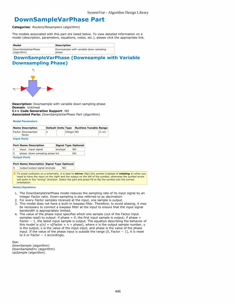
SystemVue - Algorithm Design Library
446
DownSampleVarPhase PartCategories: Routers/Resamplers (algorithm)
The models associated with this part are listed below. To view detailed information on amodel (description, parameters, equations, notes, etc.), please click the appropriate link.
Model Description
DownSampleVarPhase(algorithm)
Downsample with variable down samplingphase
DownSampleVarPhase (Downsample with VariableDownsampling Phase)
Description: Downsample with variable down sampling phaseDomain: UntimedC++ Code Generation Support: NOAssociated Parts: DownSampleVarPhase Part (algorithm)
Model Parameters
Name Description Default Units Type Runtime Tunable Range
Factor Downsamplefactor
2 Integer NO [1:∞)
Input Ports
Port Name Description Signal Type Optional
1 input input signal anytype NO
2 phase down sampling phase int NO
Output Ports
Port Name Description Signal Type Optional
3 output output signal anytype NO
To avoid confusion on a schematic, it is best to mirror (flip) this symbol (instead of rotating it) when youneed to have the input on the right and the output on the left of the symbol; otherwise the symbol arrowwill point in the "wrong" direction. Select the part and press F6 to flip the symbol into the correctorientation.
Notes/Equations
The DownSampleVarPhase model reduces the sampling rate of its input signal by an1.integer Factor ratio. Down-sampling is also referred to as decimation.For every Factor samples received at the input, one sample is output.2.This model does not have a built-in lowpass filter. Therefore, to avoid aliasing, it may3.be necessary to connect a lowpass filter at the input to ensure that the input signalbandwidth is appropriately limited.The value of the phase input specifies which one sample (out of the Factor input4.samples read) to output: if phase = 0, the first input sample is output; if phase =Factor − 1, the latest input sample is output. The equation describing the behavior ofthis model is y[n] = x[Factor × n + phase], where n is the output sample number, yis the output, x is the value of the input input, and phase is the value of the phaseinput. If the value of the phase input is outside the range [0, Factor − 1], it is resetto 0 or Factor − 1 accordingly.
See:DownSample (algorithm)DownSampleEnv (algorithm)UpSample (algorithm)

SystemVue - Algorithm Design Library
447
Latch PartCategories: Routers/Resamplers (algorithm)
The models associated with this part are listed below. To view detailed information on amodel (description, parameters, equations, notes, etc.), please click the appropriate link.
Model Description
Latch(algorithm)
Data Latch with ClockControl

SystemVue - Algorithm Design Library
448
Latch
Description: Data Latch with Clock ControlDomain: UntimedC++ Code Generation Support: NOAssociated Parts: Latch Part (algorithm)
Input Ports
Port Name Signal Type Optional
1 input anytype NO
2 clock int NO
Output Ports
Port Name Signal Type Optional
3 output anytype NO
Notes/Equations
The Latch model implements a level triggered latch.1.It reads 1 sample from the input and clock inputs and writes 1 sample to the output2.output.When the clock input is high (non-zero), it stores the value of the input input to its3.internal memory and it also writes this value to its output.When the clock input is low (zero), it outputs the value it has stored in its internal4.memory.If you want to implement an edge triggered latch you can convert a clock signal to an5.impulse train by processing it through an edge detection algorithm as shown below.

SystemVue - Algorithm Design Library
449

SystemVue - Algorithm Design Library
450
Mux PartCategories: C++ Code Generation (algorithm), Routers/Resamplers (algorithm)
The models associated with this part are listed below. To view detailed information on amodel (description, parameters, equations, notes, etc.), please click the appropriate link.
Model Description
Mux(algorithm)
Data Multiplexer
Mux (Data Multiplexer)
Description: Data MultiplexerDomain: UntimedC++ Code Generation Support: YES (see Note)Associated Parts: Mux Part (algorithm)
Model Parameters
Name Description Default Units Type Runtime Tunable Range
BlockSize Number of data items in a block 1 Integer NO [1:∞)
Input Ports
Port Name Signal Type Optional
1 control int NO
2 input multiple anytype NO
Output Ports
Port Name Signal Type Optional
3 output anytype NO
NoteThis model does not support C++ code generation if the port type is resolved to envelope signal (sim) orvariant (sim).
Notes/Equations
One of N inputs is multiplexed to the output. N is the number of input connections.1.BlockSize samples are consumed on each input. Only one of these blocks as2.determined by the control input is copied to the output.Integer values from 0 through N - 1 are expected at the control input. If the control3.input is outside this range, the simulation is terminated with an error message.
See:DeMux (algorithm)

SystemVue - Algorithm Design Library
451
OrderTwoInt PartCategories: Routers/Resamplers (algorithm)
The models associated with this part are listed below. To view detailed information on amodel (description, parameters, equations, notes, etc.), please click the appropriate link.
Model Description
OrderTwoInt(algorithm)
Ordered Two Integer Min/Max Function
OrderTwoInt (Ordered Two Integer Min/MaxFunction)
Description: Ordered Two Integer Min/Max FunctionDomain: UntimedC++ Code Generation Support: NOAssociated Parts: OrderTwoInt Part (algorithm)
Input Ports
Port Name Signal Type Optional
1 upper int NO
2 lower int NO
Output Ports
Port Name Signal Type Optional
3 greater int NO
4 lesser int NO
Notes/Equations
OrderTwoInt takes two inputs and outputs the greater and lesser of the two inputs.1.
where:x 1 is the upper input
x 2 is the lower input
y 1 is the greater output
y 2 is the lesser output
For an input sample, one sample is output.2.
See:Mux (algorithm)DeMux (algorithm)

SystemVue - Algorithm Design Library
452
Repeat PartCategories: C++ Code Generation (algorithm), Routers/Resamplers (algorithm)
The models associated with this part are listed below. To view detailed information on amodel (description, parameters, equations, notes, etc.), please click the appropriate link.
Model Description
Repeat(algorithm)
Data Repeater

SystemVue - Algorithm Design Library
453
Repeat
Description: Data RepeaterDomain: UntimedC++ Code Generation Support: YES (see Note)Associated Parts: Repeat Part (algorithm)
Model Parameters
Name Description Default Units Type Runtime Tunable Range
NumTimes Repetition factor 2 Integer NO [1:∞)
BlockSize Number of data items in a block 1 Integer NO [1:∞)
Input Ports
Port Name Signal Type Optional
1 input anytype NO
Output Ports
Port Name Signal Type Optional
2 output anytype NO
NoteThis model does not support C++ code generation if the port type is resolved to envelope signal (sim) orvariant (sim).
Notes/Equations
Repeat copies BlockSize number of inputs to the output NumTimes.1.For every BlockSize number of inputs, there are BlockSize × NumTimes number of2.outputs.This model is useful when a block of inputs needs upsampling.3.
Note on large upsampling factorsEach repeater require a buffer of NumTimes number of BlockSize × samples. For a large NumTimes value,memory requirements may prevent a simulation. The way around this problem is to substitute a cascadeof repeaters. For example, a NumTimes of 10 6 would require a buffer of 10 6 BlockSize × samples. If acascade of two repeater were used, then each NumTimes could be 10 3 which would require a total bufferequivalent of 2 × 10 3 BlockSize × samples. If a cascade of three repeater were used, then eachNumTimes could be 10 2 which would require a total buffer equivalent of 3 × 10 2 BlockSize × samples.
See:DownSample (algorithm)UpSample (algorithm)

SystemVue - Algorithm Design Library
454
ResamplerRC PartCategories: C++ Code Generation (algorithm), Routers/Resamplers (algorithm)
The models associated with this part are listed below. To view detailed information on amodel (description, parameters, equations, notes, etc.), please click the appropriate link.
Model Description
ResamplerRC(algorithm)
Resampler with Raised CosineFilter
ResamplerRC (Resampler with Raised Cosine Filter)
Description: Resampler with Raised Cosine FilterDomain: UntimedC++ Code Generation Support: YESAssociated Parts: ResamplerRC Part (algorithm)
Model Parameters
Name Description Default Units Type Runtime Tunable
Decimation Decimation ratio 1 Integer NO
DecimationPhase Decimation phase 0 Integer NO
Interpolation Interpolationratio
16 Integer NO
Length Number of taps 64 Integer NO
ExcessBW Excess bandwidth 1 Float YES
Input Ports
Port Name Signal Type Optional
1 input real NO
Output Ports
Port Name Signal Type Optional
2 output real NO
Notes/Equations
The ResamplerRC implements a rational ratio resampler that uses a raised cosine1.filter as the interpolating filter.For every Decimation number of input samples, Interpolation number of filtered2.values are output.For more information on the multi-rate implementation, see FIR (algorithm).3.DecimationPhase is equivalent to the Phase parameter of the DownSample4.(algorithm) part. If DecimationPhase is 0 (default), the earliest outputs of thedecimation block are decimated.The Length parameter defines the number of taps in the raised cosine filter.5.ExcessBW parameter defines the excess bandwidth for the raised cosine filter. This6.value is often referred as the rolloff or the alpha of the raised cosine filter.The impulse response of an ideal raised cosine filter is given by7.
The ideal impulse response is centered at 0. Since only causal filters areimplemented, the actual impulse response used is
The impulse response is truncated outside the range [0, L-1].
References
E. A. Lee and D. G. Messerchmitt, Digital Communication, Kluwer Academic1.Publishers, Boston, 1988.I. Korn, Digital Communications, Van Nostrand Reinhold, New York, 1985.2.

SystemVue - Algorithm Design Library
455
See:FIR (algorithm)

SystemVue - Algorithm Design Library
456
SampleHold PartCategories: Routers/Resamplers (algorithm)
The models associated with this part are listed below. To view detailed information on amodel (description, parameters, equations, notes, etc.), please click the appropriate link.
Model Description
SampleHold(algorithm)
Sample and hold with clockcontrol

SystemVue - Algorithm Design Library
457
SampleHold
Description: Sample and hold with clock controlDomain: UntimedC++ Code Generation Support: NOAssociated Parts: SampleHold Part (algorithm)
Input Ports
Port Name Signal Type Optional
1 input anytype NO
2 clock int NO
Output Ports
Port Name Signal Type Optional
3 output anytype NO
Notes/Equations
The SampleHold model sets its output to the input when the clock is non-zero.1.This model reads 1 sample from the input and clock and writes 1 sample to the2.output.

SystemVue - Algorithm Design Library
458
SetSampleRate PartCategories: Routers/Resamplers (algorithm)
The models associated with this part are listed below. To view detailed information on amodel (description, parameters, equations, notes, etc.), please click the appropriate link.
Model Description
SetSampleRate(algorithm)
Set Signal Sample Rate
SetSampleRate (Set Signal Sample Rate)
Description: Set Signal Sample RateDomain: TimedC++ Code Generation Support: NOAssociated Parts: SetSampleRate Part (algorithm)
Model Parameters
Name Description Default Units Type Runtime Tunable Range
SampleRate Sample rate Sample_Rate Hz Float NO (0:∞)
Input Ports
Port Name Signal Type Optional
1 input anytype NO
Output Ports
Port Name Signal Type Optional
2 output anytype NO
Notes/Equations
The SetSampleRate model associates a sample rate with the input data and sets the1.output with that data and its associated sample rate.This model reads 1 sample from the input and writes 1 sample to the output.2.The output sample rate generates time values for the output.3.For a discussion on the precision of the time values, see Sources Category4.(algorithm).A consistency check on the multirate graph will flag implementation problems.5.

SystemVue - Algorithm Design Library
459
Trainer PartCategories: Routers/Resamplers (algorithm)
The models associated with this part are listed below. To view detailed information on amodel (description, parameters, equations, notes, etc.), please click the appropriate link.
Model Description
Trainer(algorithm)
Initial SampleTrainer
Trainer (Initial Sample Trainer)
Description: Initial Sample TrainerDomain: UntimedC++ Code Generation Support: NOAssociated Parts: Trainer Part (algorithm)
Model Parameters
Name Description Default Units Type Runtime Tunable Range
TrainLength Number of training samples to use 100 Integer NO [0:∞)
Input Ports
Port Name Signal Type Optional
1 train anytype NO
2 decision anytype NO
Output Ports
Port Name Signal Type Optional
3 output anytype NO
Notes/Equations
Trainer passes the value of the training input to the output for the first TrainLength1.samples, then passes the decision input to the output.For every input, there is an output.2.During the startup phase, the decision inputs are discarded. After the startup phase,3.the training inputs are discarded.This component is designed for use with adaptive equalizers that require a training4.sequence at startup, but it can be used whenever one sequence is used during astartup phase, and another sequence after that.

SystemVue - Algorithm Design Library
460
UpSample PartCategories: Routers/Resamplers (algorithm)
The models associated with this part are listed below. To view detailed information on amodel (description, parameters, equations, notes, etc.), please click the appropriate link.
Model Description
UpSample (algorithm) Up Sampler
UpSampleEnv(algorithm)
Up Sampler for Envelope Signal
UpSampleFxp (hardware) Fixed Point UpSample
UpSample (Upsampler)
Description: Up SamplerDomain: UntimedC++ Code Generation Support: NOAssociated Parts: UpSample Part (algorithm)
Model Parameters
Name Description Default Units Type RuntimeTunable
Range
Factor Number of samples produced 2 Integer NO [1:∞)
Mode Mode method: Insert zeros, Hold sample Insertzeros
Enumeration YES
Phase Where to put the input in the output block.Visible when Mode mode is Insert zeros
0 Integer YES [0:Factor-1]
Input Ports
Port Name Description Signal Type Optional
1 input input signal anytype NO
Output Ports
Port Name Description Signal Type Optional
2 output output signal anytype NO
To avoid confusion on a schematic, it is best to mirror (flip) this symbol (instead of rotating it) when youneed to have the input on the right and the output on the left of the symbol; otherwise the symbol arrowwill point in the "wrong" direction. Select the part and press F6 to flip the symbol into the correctorientation.
Notes/Equations
UpSample increases the sample rate of the input signal by Factor.1.This model reads one sample from the input and writes Factor number of samples to2.the output.If Mode is Insert zeros, the inserted output samples have the zero value of the input3.type. Otherwise, the output samples have the same value as the most recent input.For Insert zeros mode only, the Phase parameter specifies where to place the input4.sample in a block of Factor output samples. Phase number of zeros are output firstfollowed by the input value followed by (Factor - 1) - Phase number of zeros.Examples follow.
If Phase is zero, the input value is output first followed by Factor - 1 number of1.zeros.If Phase is Factor - 1, Factor - 1 number of zeros are output first followed by the2.input value.

SystemVue - Algorithm Design Library
461
Note on large upsampling factorsEach upsampler require a buffer of Factor number of samples. For a large Factor value, memoryrequirements may prevent a simulation. The way around this problem is to substitute a cascade ofupsamplers. For example, a Factor of 10 6 would require a buffer of 10 6 samples. If a cascade of twoupsamplers were used, then each Factor could be 10 3 which would require a total buffer equivalent of 2 ×10 3 samples. If a cascade of three upsamplers were used, then each Factor could be 10 2 which wouldrequire a total buffer equivalent of 3 × 10 2 samples.If a nonzero Phase were to be used, the Phase would have to be deconstructed into Phase values for eachcascaded upsampler. Let an upsample part have a Factor of 10 6 and a Phase of 123456. The upsampler issubstituted by 3 upsamplers each having a Factor of 10 2. The first upsampler would have a Phase of 12,the second upsampler would have a Phase of 34 and the third sampler would have a Phase of 56.
See:DownSample (algorithm)Repeat (algorithm)

SystemVue - Algorithm Design Library
462
Signal ProcessingThe Signal Processing library provides parts that implement signal processing algorithms,like FFT, Quantization, Compress/Expand, etc.
ContentsAdaptLinQuant Part (algorithm)AutoCorr Part (algorithm)Average Part (algorithm)AverageCxWOffset Part (algorithm)BitDeformatter Part (algorithm)BitFormatter Part (algorithm)Chop Part (algorithm)ChopVarOffset Part (algorithm)Compress Part (algorithm)Convolve Part (algorithm)CrossCorr Part (algorithm)CyclicShift Part (algorithm)DeadZone Part (algorithm)Delay Part (algorithm)DTFT Part (algorithm)Expand Part (algorithm)FFT Cx Part (algorithm)FFT SHift Part (algorithm)Filter Part (algorithm)GeometricMean Part (algorithm)Hysteresis Part (algorithm)Limit Part (algorithm)LinearQuantizer Part (algorithm)LookUpTable Part (algorithm)MaxMin Part (algorithm)PattMatch Part (algorithm)PcwzLinear Part (algorithm)Quantizer Part (algorithm)Quantizer2D Part (algorithm)Reverse Part (algorithm)SchmittTrig Part (algorithm)SlidWinAvg Part (algorithm)TimeDelay Part (algorithm)TimeSynchronizer Part (algorithm)Transpose Part (algorithm)VarDelay Part (algorithm)Variance Part (algorithm)

SystemVue - Algorithm Design Library
463
AdaptLinQuant PartCategories: Signal Processing (algorithm)
The models associated with this part are listed below. To view detailed information on amodel (description, parameters, equations, notes, etc.), please click the appropriate link.
Model Description
AdaptLinQuant(algorithm)
Adaptive Linear Quantizer
AdaptLinQuant (Adaptive Linear Quantizer)
Description: Adaptive Linear QuantizerDomain: UntimedC++ Code Generation Support: NOAssociated Parts: AdaptLinQuant Part (algorithm)
Model Parameters
Name Description Default Units Type Runtime Tunable Range
Bits Number of bits 8 Integer YES [1:31]
Input Ports
Port Name Signal Type Optional
1 input real NO
2 inStep real NO
Output Ports
Port Name Signal Type Optional
3 amplitude real NO
4 outStep real NO
5 stepLevel int NO
Notes/Equations
Input is quantized to 2 Bits number of levels in a plan described as odd symmetric1.about zero midrise.For each model execution, one sample is read at each input and one sample is2.written to each output.Quantization levels are uniformly spaced by inStep and symmetric about zero.3.Therefore, the high quantization level is (2 Bits − 1)(inStep / 2), the low quantizationlevel is set to −high. Zero is not a quantization level.Input is held to a value between low and high and rounded to the nearest4.quantization level.Quantized input is output on the amplitude port. Its quantization index is output on5.the stepLevel port as an integer between 0 and 2 Bits − 1.inStep is copied to the outStep port.6.
See:LinearQuantizer (algorithm)Quantizer (algorithm)Quantizer2D (algorithm)

SystemVue - Algorithm Design Library
464
AutoCorr PartCategories: Signal Processing (algorithm)
The models associated with this part are listed below. To view detailed information on amodel (description, parameters, equations, notes, etc.), please click the appropriate link.
Model Description
AutoCorr(algorithm)
AutocorrelationEstimator
AutoCorr (Autocorrelation Estimator)
Description: Autocorrelation EstimatorDomain: UntimedC++ Code Generation Support: NOAssociated Parts: AutoCorr Part (algorithm)
Model Parameters
Name Description Default Units Type RuntimeTunable
Range Symbol
CorrelationType Correlation method:NonCircular,Circular
Circular Enumeration YES
CorrelationLength Number of inputsamples
511 Integer NO [1:∞) N
StartLag Low lag limit tooutput
-255 Integer NO (-N:L<sub>h</sub>]
Ll
StopLag High lag limit tooutput
255 Integer NO [L<sub>l</sub>:N) Lh
Normalization Correlation estimatenormalization:None, UnBiased,Biased
None Enumeration YES
Input Ports
Port Name Description Signal Type Optional
1 input input signal real NO
Output Ports
Port Name Description Signal Type Optional
2 output output signal real NO
Notes/Equations
AutoCorr estimates the autocorrelation function of the input.1.The part inputs N samples and outputs L l + L h + 1 autocorrelation values.2.
r x (k) is the estimated autocorrelation function of N input samples and is evaluated3.
for a k from L l, ... , L h.
r x (L l) is output first, and r x (L h) is output last.4.
If CorrelationType is NonCircular, then5.r x (k) = sum { x (i) x (i + k) } for input x and i = 1, ... , N. For p < 1 or p > N, x
(p) is 0.Otherwise, the CorrelationType is Circular, thenr x (k) = sum { x (i) x (i + k) } for input x and i = 1, ... , N. For p < 1 or p > N, x
(p) is x ( ( (p - 1) modulo N) + 1 ). Define -1 modulo N as N - 1, and so on.Additionally, UnBiased and Biased autocorrelation estimates are supported.6.
If CorrelationType is NonCircular, then for UnBiased Normalization, r x (k) is
divided by N - | k |. For Biased Normalization, r x (k) is divided by N.
If CorrelationType is Circular, then for UnBiased or Biased Normalization, r x (k)
is divided by N.A typical application of AutoCorr is to find periodicities in N samples of input. For this7.application, set CorrelationType to Circular.
See:CrossCorr (algorithm)

SystemVue - Algorithm Design Library
465
References
A. V. Oppenheim and R. W. Schafer, Discrete-Time Signal Processing, Prentice-Hall:1.Englewood Cliffs, NJ, 1989.
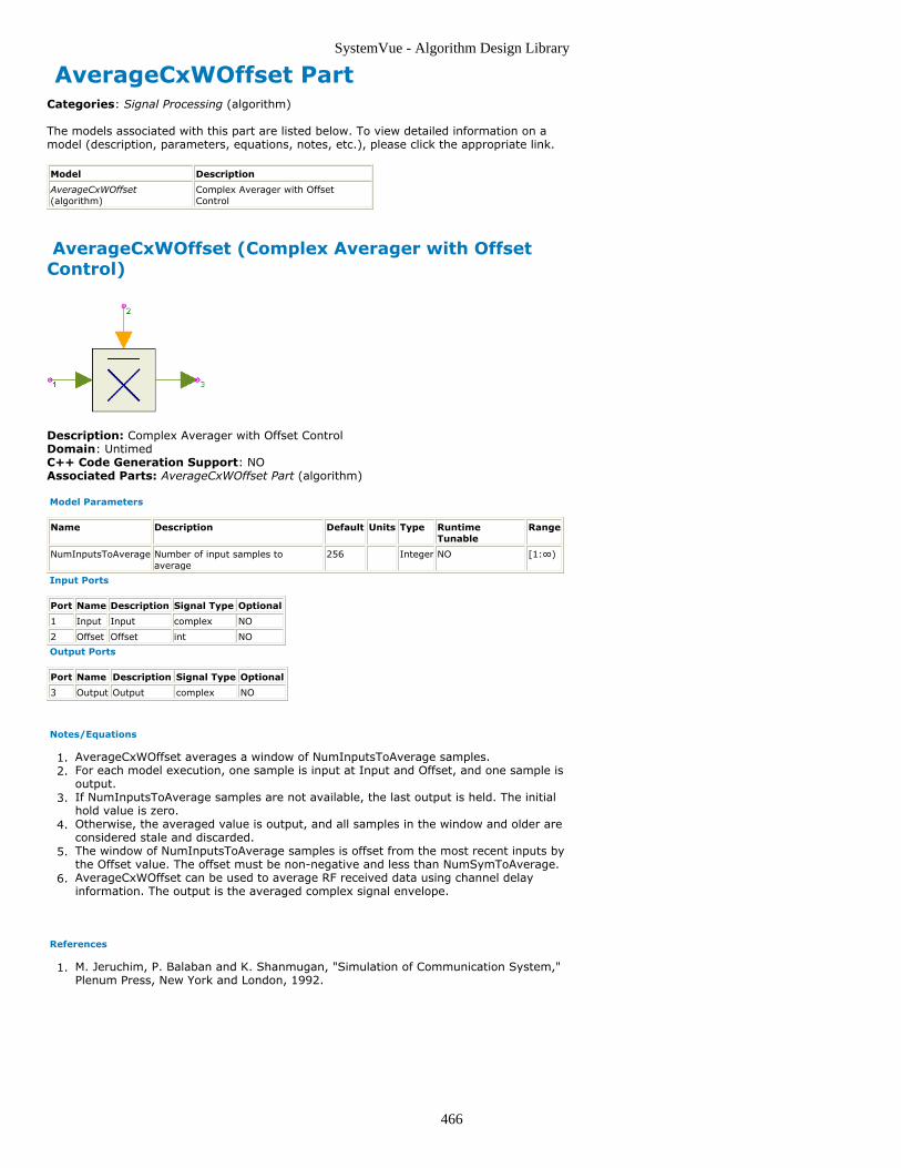
SystemVue - Algorithm Design Library
466
AverageCxWOffset PartCategories: Signal Processing (algorithm)
The models associated with this part are listed below. To view detailed information on amodel (description, parameters, equations, notes, etc.), please click the appropriate link.
Model Description
AverageCxWOffset(algorithm)
Complex Averager with OffsetControl
AverageCxWOffset (Complex Averager with OffsetControl)
Description: Complex Averager with Offset ControlDomain: UntimedC++ Code Generation Support: NOAssociated Parts: AverageCxWOffset Part (algorithm)
Model Parameters
Name Description Default Units Type RuntimeTunable
Range
NumInputsToAverage Number of input samples toaverage
256 Integer NO [1:∞)
Input Ports
Port Name Description Signal Type Optional
1 Input Input complex NO
2 Offset Offset int NO
Output Ports
Port Name Description Signal Type Optional
3 Output Output complex NO
Notes/Equations
AverageCxWOffset averages a window of NumInputsToAverage samples.1.For each model execution, one sample is input at Input and Offset, and one sample is2.output.If NumInputsToAverage samples are not available, the last output is held. The initial3.hold value is zero.Otherwise, the averaged value is output, and all samples in the window and older are4.considered stale and discarded.The window of NumInputsToAverage samples is offset from the most recent inputs by5.the Offset value. The offset must be non-negative and less than NumSymToAverage.AverageCxWOffset can be used to average RF received data using channel delay6.information. The output is the averaged complex signal envelope.
References
M. Jeruchim, P. Balaban and K. Shanmugan, "Simulation of Communication System,"1.Plenum Press, New York and London, 1992.
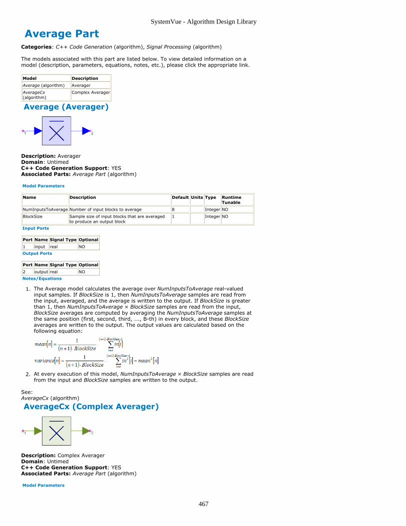
SystemVue - Algorithm Design Library
467
Average PartCategories: C++ Code Generation (algorithm), Signal Processing (algorithm)
The models associated with this part are listed below. To view detailed information on amodel (description, parameters, equations, notes, etc.), please click the appropriate link.
Model Description
Average (algorithm) Averager
AverageCx(algorithm)
Complex Averager
Average (Averager)
Description: AveragerDomain: UntimedC++ Code Generation Support: YESAssociated Parts: Average Part (algorithm)
Model Parameters
Name Description Default Units Type RuntimeTunable
NumInputsToAverage Number of input blocks to average 8 Integer NO
BlockSize Sample size of input blocks that are averagedto produce an output block
1 Integer NO
Input Ports
Port Name Signal Type Optional
1 input real NO
Output Ports
Port Name Signal Type Optional
2 output real NO
Notes/Equations
The Average model calculates the average over NumInputsToAverage real-valued1.input samples. If BlockSize is 1, then NumInputsToAverage samples are read fromthe input, averaged, and the average is written to the output. If BlockSize is greaterthan 1, then NumInputsToAverage × BlockSize samples are read from the input,BlockSize averages are computed by averaging the NumInputsToAverage samples atthe same position (first, second, third, ..., B-th) in every block, and these BlockSizeaverages are written to the output. The output values are calculated based on thefollowing equation:
At every execution of this model, NumInputsToAverage × BlockSize samples are read2.from the input and BlockSize samples are written to the output.
See:AverageCx (algorithm)
AverageCx (Complex Averager)
Description: Complex AveragerDomain: UntimedC++ Code Generation Support: YESAssociated Parts: Average Part (algorithm)
Model Parameters

SystemVue - Algorithm Design Library
468
Name Description Default Units Type RuntimeTunable
NumInputsToAverage Number of input blocks to average 8 Integer NO
BlockSize Sample size of input blocks that are averagedto produce an output block
1 Integer NO
Input Ports
Port Name Signal Type Optional
1 input complex NO
Output Ports
Port Name Signal Type Optional
2 output complex NO
Notes/Equations
The AverageCx model calculates the average over NumInputsToAverage complex-1.valued input samples. If BlockSize is 1, then NumInputsToAverage samples are readfrom the input, averaged, and the average is written to the output. If BlockSize isgreater than 1, then NumInputsToAverage × BlockSize samples are read from theinput, BlockSize averages are computed by averaging the NumInputsToAveragesamples at the same position (first, second, third, ..., B-th) in every block, and theseBlockSize averages are written to the output. The output values are calculated basedon the following equation:
At every execution of this model, NumInputsToAverage × BlockSize samples are read2.from the input and BlockSize samples are written to the output.
See:Average (algorithm)

SystemVue - Algorithm Design Library
469
BitDeformatter PartCategories: C++ Code Generation (algorithm), Signal Processing (algorithm), TypeConverters (algorithm)
The models associated with this part are listed below. To view detailed information on amodel (description, parameters, equations, notes, etc.), please click the appropriate link.
Model Description
BitDeformatter(algorithm)
NRZ/RZ Symbol to BitConverter
BitDeformatter (NRZ/RZ Symbol to Bit Converter)
Description: NRZ/RZ Symbol to Bit ConverterDomain: UntimedC++ Code Generation Support: YESAssociated Parts: BitDeformatter Part (algorithm)
Model Parameters
Name Description Default Units Type Runtime Tunable
SamplesPerBit Number of input samples per bit 1 Integer NO
Format Format for input signal: NRZ,RZ
NRZ Enumeration NO
LogicZeroLevel Voltage for bit value zero -1 V Float YES
LogicOneLevel Voltage for bit value one 1 V Float YES
Input Ports
Port Name Signal Type Optional
1 input real NO
Output Ports
Port Name Signal Type Optional
2 output boolean NO
Notes/Equations
The BitDeformatter converts input NRZ/RZ symbols to output bits.1.This model reads SamplesPerBit samples from input representing one NRZ/RZ2.symbol and interprets it using the Format parameter to write 1 sample to output as abit value that has a logic level defined by LogicZeroLevel and LogicOneLevel.Format specifies the pulse-code modulation (PCM) waveform type: Nonreturn-to-3.zero (NRZ) or Return-to-zero (RZ). Unipolar RZ and Bipolar RZ are specified withappropriate values for parameters LogicZeroLevel and LogicOneLevel.For NRZ, the sampled input waveform is averaged. The averaged value that is closer4.to LogicZeroLevel than LogicOneLevel outputs a zero bit, otherwise a one bit isoutput.For RZ, the SamplerPerBit parameter must be a multiple of two as the format returns5.to "zero" in the last half of the waveform. The sampled input waveform is separatelyaveraged in the first and second half of the bit period. The averaged "zero" provide azero reference for the bit period. If the differential value for the bit period is closer toLogicZeroLevel than LogicOneLevel, a zero bit is output, otherwise a one bit isoutput.
See:BitFormatter (algorithm)
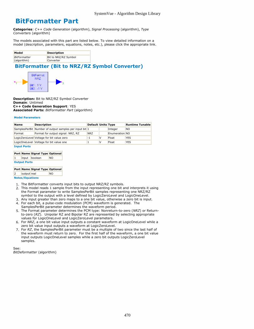
SystemVue - Algorithm Design Library
470
BitFormatter PartCategories: C++ Code Generation (algorithm), Signal Processing (algorithm), TypeConverters (algorithm)
The models associated with this part are listed below. To view detailed information on amodel (description, parameters, equations, notes, etc.), please click the appropriate link.
Model Description
BitFormatter(algorithm)
Bit to NRZ/RZ SymbolConverter
BitFormatter (Bit to NRZ/RZ Symbol Converter)
Description: Bit to NRZ/RZ Symbol ConverterDomain: UntimedC++ Code Generation Support: YESAssociated Parts: BitFormatter Part (algorithm)
Model Parameters
Name Description Default Units Type Runtime Tunable
SamplesPerBit Number of output samples per input bit 1 Integer NO
Format Format for output signal: NRZ, RZ NRZ Enumeration NO
LogicZeroLevel Voltage for bit value zero -1 V Float YES
LogicOneLevel Voltage for bit value one 1 V Float YES
Input Ports
Port Name Signal Type Optional
1 input boolean NO
Output Ports
Port Name Signal Type Optional
2 output real NO
Notes/Equations
The BitFormatter converts input bits to output NRZ/RZ symbols.1.This model reads 1 sample from the input representing one bit and interprets it using2.the Format parameter to write SamplesPerBit samples representing one NRZ/RZsymbol to the output with a level defined by LogicZeroLevel and LogicOneLevel.Any input greater than zero maps to a one bit value, otherwise a zero bit is input. 3.For each bit, a pulse-code modulation (PCM) waveform is generated. The4.SamplesPerBit parameter determines the waveform period.The Format parameter determines the PCM type: Nonreturn-to-zero (NRZ) or Return-5.to-zero (RZ). Unipolar RZ and Bipolar RZ are represented by selecting appropriatevalues for LogicOneLevel and LogicZeroLevel parameters.For NRZ, a one bit value input outputs a constant waveform at LogicOneLevel while a6.zero bit value input outputs a waveform at LogicZeroLevel.For RZ, the SamplesPerBit parameter must be a multiple of two since the last half of7.the waveform must return to zero. For the first half of the waveform, a one bit valueinput outputs LogicOneLevel samples while a zero bit outputs LogicZeroLevelsamples.
See:BitDeformatter (algorithm)
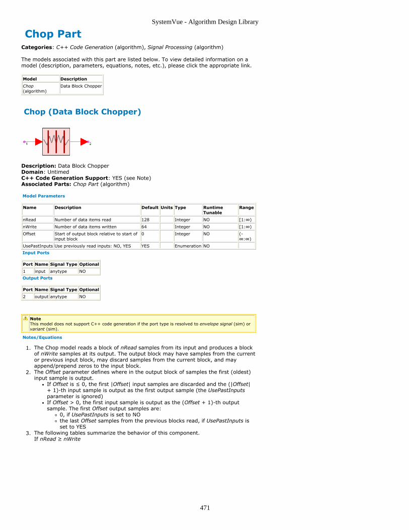
SystemVue - Algorithm Design Library
471
Chop PartCategories: C++ Code Generation (algorithm), Signal Processing (algorithm)
The models associated with this part are listed below. To view detailed information on amodel (description, parameters, equations, notes, etc.), please click the appropriate link.
Model Description
Chop(algorithm)
Data Block Chopper
Chop (Data Block Chopper)
Description: Data Block ChopperDomain: UntimedC++ Code Generation Support: YES (see Note)Associated Parts: Chop Part (algorithm)
Model Parameters
Name Description Default Units Type RuntimeTunable
Range
nRead Number of data items read 128 Integer NO [1:∞)
nWrite Number of data items written 64 Integer NO [1:∞)
Offset Start of output block relative to start ofinput block
0 Integer NO (-∞:∞)
UsePastInputs Use previously read inputs: NO, YES YES Enumeration NO
Input Ports
Port Name Signal Type Optional
1 input anytype NO
Output Ports
Port Name Signal Type Optional
2 output anytype NO
NoteThis model does not support C++ code generation if the port type is resolved to envelope signal (sim) orvariant (sim).
Notes/Equations
The Chop model reads a block of nRead samples from its input and produces a block1.of nWrite samples at its output. The output block may have samples from the currentor previous input block, may discard samples from the current block, and mayappend/prepend zeros to the input block.The Offset parameter defines where in the output block of samples the first (oldest)2.input sample is output.
If Offset is ≤ 0, the first |Offset| input samples are discarded and the (|Offset|+ 1)-th input sample is output as the first output sample (the UsePastInputsparameter is ignored)If Offset > 0, the first input sample is output as the (Offset + 1)-th outputsample. The first Offset output samples are:
0, if UsePastInputs is set to NOthe last Offset samples from the previous blocks read, if UsePastInputs isset to YES
The following tables summarize the behavior of this component.3.If nRead ≥ nWrite

SystemVue - Algorithm Design Library
472
Case Offset UsePastInputs nWrite ≤nRead − |Offset|
Output
1 (−∞, −nRead]
NO or YES will alwaysbe FALSE
all zeros
2 (−nRead,0]
NO or YES TRUE discard the first |Offset| input samples, output the nextnWrite input samples
3 (−nRead,0]
NO or YES FALSE discard the first |Offset| input samples, output the next(nRead − |Offset|) input samples followed by (nWrite −(nRead − |Offset|)) zeros
4 (0,nWrite)
NO TRUE orFALSE
output Offset zeros followed by the first (nWrite − Offset) input samples
5 (0,nWrite)
YES TRUE orFALSE
output the last Offset samples of the previously readinput block followed by the first (nWrite − Offset) inputsamples
6 [nWrite,∞)
NO TRUE orFALSE
all zeros
7 [nWrite,∞)
YES TRUE orFALSE
output from the (nRead − Offset + 1)-th to (nRead −Offset + nWrite)-th samples of the previously read inputblock (for the first block the previous block is assumedto be all zeros)
If nRead < nWrite
Case Offset UsePastInputs nRead ≤nWrite − |Offset|
Output
8 (−∞, −nRead]
NO or YES TRUE orFALSE
all zeros
9 (−nRead, 0]
NO or YES TRUE orFALSE
discard the first |Offset| input samples, output thenext (nRead − |Offset|) input samples followed by (nWrite − (nRead − |Offset|)) zeros
10 (0,nWrite)
NO TRUE output Offset zeros followed by the nRead inputsamples followed by (nWrite − nRead − Offset) zeros
11 (0,nWrite)
NO FALSE output Offset zeros followed by the first (nWrite −Offset) input samples
12 (0,nWrite)
YES TRUE output the last Offset samples of the previously readinput block followed by the nRead input samplesfollowed by (nWrite − nRead − Offset) zeros
13 (0,nWrite)
YES FALSE output the last Offset samples of the previously readinput block(s) followed by the first (nWrite − Offset)input samples
14 [nWrite,∞)
NO will always beFALSE
all zeros
15 [nWrite,∞)
YES will always beFALSE
output the last nWrite samples of the previously readinput block(s) (for the first block the previous blocksare assumed to be all zeros)
Here are some examples. In all of these examples the input is assumed to be a ramp4.signal with initial value of 1 and step 1 (1, 2, 3, 4, 5, 6, ...).Case nRead nWrite Offset UsePastInputs Output
1 10 5 -10 (orsmaller)
NO or YES 0, 0, 0, 0, 0, 0, ...
2 10 3 -5 NO or YES 6, 7, 8, 16, 17, 18, 26, 27, 28, ...
3 10 5 -7 NO or YES 8, 9, 10, 0, 0, 18, 19, 20, 0, 0, 28, 29, 30, 0, 0, ...
4 10 5 2 NO 0, 0, 1, 2, 3, 0, 0, 11, 12, 13, 0, 0, 21, 22, 23, ...
5 10 5 2 YES 0, 0, 1, 2, 3, 9, 10, 11, 12, 13, 19, 20, 21, 22, 23,...
6 10 5 5 (orbigger)
NO 0, 0, 0, 0, 0, 0, ...
7 10 5 5 YES 0, 0, 0, 0, 0, 6, 7, 8, 9, 10, 16, 16, 18, 19, 20, ...
7 10 5 7 YES 0, 0, 0, 0, 0, 4, 5, 6, 7, 8, 14, 15, 16, 17, 18, ...
8 5 10 -5 (orsmaller)
NO or YES 0, 0, 0, 0, 0, 0, ...
9 5 10 -3 NO or YES 4, 5, 0, 0, 0, 0, 0, 0, 0, 0, 9, 10, 0, 0, 0, 0, 0, 0, 0,0, 14, 15, 0, 0, 0, 0, 0, 0, 0, 0, ...
10 5 10 3 N0 0, 0, 0, 1, 2, 3, 4, 5, 0, 0, 0, 0, 0, 6, 7, 8, 9, 10, 0,0, 0, 0, 0, 11, 12, 13, 14, 15, 0, 0, ...
11 5 10 7 N0 0, 0, 0, 0, 0, 0, 0, 1, 2, 3, 0, 0, 0, 0, 0, 0, 0, 6, 7,8, 0, 0, 0, 0, 0, 0, 0, 11, 12, 13, ...
12 5 10 3 YES 0, 0, 0, 1, 2, 3, 4, 5, 0, 0, 3, 4, 5, 6, 7, 8, 9, 10, 0,0, 8, 9, 10, 11, 12, 13, 14, 15, 0, 0, ...
13 5 10 7 YES 0, 0, 0, 0, 0, 0, 0, 1, 2, 3, 0, 0, 1, 2, 3, 4, 5, 6, 7,8, 4, 5, 6, 7, 8, 9, 10, 11, 12, 13, ...
14 5 10 10 (orbigger)
NO 0, 0, 0, 0, 0, 0, ...
15 3 5 5 YES 0, 0, 0, 0, 0, 0, 0, 1, 2, 3, 2, 3, 4, 5, 6, 5, 6, 7, 8,9, ...
Common uses of the Chop component include:5.

SystemVue - Algorithm Design Library
473
Discard samples from the beginning of a block of data: Offset should be set to −N, where N is the number of samples that need to be discarded and nWrite shouldbe set to nRead − N.Discard samples from the end of a block of data: Offset should be set to 0 andnWrite should be set to nRead − N, where N is the number of samples that needto be discarded.Discard samples from both the beginning and the end of a block of data: Offsetshould be set to −N b, where N b is the number of samples that need to be
discarded from the beginning of the block and nWrite should be set to nRead −N b − N e, where N e is the number of samples that need to be discarded from
the end of the block.Prepend zeros to a block of data: Offset should be set to N , where N is thenumber of zeros to be prepended, UsePastInputs should be set to NO, andnWrite should be set to nRead + N.Append zeros to a block of data: Offset should be set to 0 and nWrite should beset to nRead + N, where N is the number of zeros to be appended.Prepend and append zeros to a block of data: Offset should be set to N p , where
N p is the number of zeros to be prepended, UsePastInputs should be set to NO,
and nWrite should be set to nRead + N p + N a, where N a is the number of
zeros to be appended.Break an input stream of samples in blocks of size N b with N o overlapping
samples: nRead should be set to N b − N o, nWrite should be set to N b, Offset
should be set to N o, and UsePastInputs should be set to YES.
See:ChopVarOffset (algorithm)
Timing
When this model is used in a timed simulation, the first sample at its output will occur attime t 0 + (nRead - 1) / SampleRate, where t 0 is the time stamp of the first input sample
and SampleRate is the sample rate of the input signal. For more information about timingsee Timing Method (sim).

SystemVue - Algorithm Design Library
474
ChopVarOffset PartCategories: C++ Code Generation (algorithm), Signal Processing (algorithm)
The models associated with this part are listed below. To view detailed information on amodel (description, parameters, equations, notes, etc.), please click the appropriate link.
Model Description
ChopVarOffset(algorithm)
Data Block Chopper with OffsetControl
ChopVarOffset (Data Block Chopper with OffsetControl)
Description: Data Block Chopper with Offset ControlDomain: UntimedC++ Code Generation Support: YES (see Note)Associated Parts: ChopVarOffset Part (algorithm)
Model Parameters
Name Description Default Units Type Runtime Tunable Range
nRead Number of data items read 128 Integer NO [1:∞)
nWrite Number of data items written 64 Integer NO [1:∞)
Input Ports
Port Name Signal Type Optional
1 input anytype NO
2 offsetCntrl int NO
Output Ports
Port Name Signal Type Optional
3 output anytype NO
NoteThis model does not support C++ code generation if the port type is resolved to envelope signal (sim) orvariant (sim).
Notes/Equations
ChopVarOffset has the same functionality as the Chop (algorithm) model except that1.the Offset parameter is determined at run time by a control input (offsetCntrl) andthe UsePastInputs parameter is assumed to be NO.The model reads a block of nRead samples from its input and produces a block of2.nWrite samples at its output.
See:Chop (algorithm)

SystemVue - Algorithm Design Library
475
Compress PartCategories: Signal Processing (algorithm)
The models associated with this part are listed below. To view detailed information on amodel (description, parameters, equations, notes, etc.), please click the appropriate link.
Model Description
Compress(algorithm)
Compression Part of a Compander
Compress (Compression Part of a Compander)
Description: Compression Part of a CompanderDomain: UntimedC++ Code Generation Support: NOAssociated Parts: Compress Part (algorithm)
Model Parameters
Name Description Default Units Type Runtime Tunable Range
CompressionType Compression law: MU-law, A-law
MU-law Enumeration YES
CompressionK Compression constant 1 Float YES
Max Maximum input value magnitude 1 Float YES (0.0:∞)
Input Ports
Port Name Signal Type Optional
1 input real NO
Output Ports
Port Name Signal Type Optional
2 output real NO
Notes/Equations
Compress performs MU-law or A-law compression.1.For every input, there one output.2.Let x′(n) = x(n) / Max, then3.MU-law:
A-law:
wherex(n) is input for sample nV M is Max
y(n) is output for sample nµ is CompressionK for MU-lawA is CompressionK for A-lawShown below is the input/output characteristic of Compress with Type = MU-law,4.CompressionK = 255 and Max = 1V.
Compress Signal Plot

SystemVue - Algorithm Design Library
476
See:Expand (algorithm)

SystemVue - Algorithm Design Library
477
Convolve PartCategories: C++ Code Generation (algorithm), Signal Processing (algorithm)
The models associated with this part are listed below. To view detailed information on amodel (description, parameters, equations, notes, etc.), please click the appropriate link.
Model Description
Convolve (algorithm) Convolution Function
ConvolveCx(algorithm)
Complex ConvolutionFunction
Convolve (Convolution Function)
Description: Convolution FunctionDomain: UntimedC++ Code Generation Support: YESAssociated Parts: Convolve Part (algorithm)
Model Parameters
Name Description Default Units Type Runtime Tunable
TruncationDepth Maximum number of terms in convolutionsum
256 Integer NO
Input Ports
Port Name Signal Type Optional
1 inA real NO
2 inB real NO
Output Ports
Port Name Signal Type Optional
3 out real NO
Notes/Equations
The Convolve model convolves two real-valued causal finite length sequences.1.
For each model execution, one sample is read from inA and inB, and one convolution2.value is output.TruncationDepth must be set to a value larger than the number of output samples of3.interest. Otherwise, the results will be unexpected after TruncationDepth samples.If one input has finite length and does not change over time, whereas the other input4.can be arbitrarily long, use the FIR (algorithm) model. Set the Taps parameter of theFIR (algorithm) model to the values of the finite length sequence.If one input has finite length and changes over time, whereas the other input can be5.arbitrarily long, use the BlockFIR (algorithm) model. BlockFIR (algorithm) allowsfiltering of a signal in fixed size blocks, where each input block is filtered with adifferent set of coefficients.
See:ConvolveCx (algorithm)
References
A. V. Oppenheim and R. W. Schafer, Discrete-Time Signal Processing, Prentice-Hall:1.Englewood Cliffs, NJ, 1989.
ConvolveCx (Complex Convolution Function)

SystemVue - Algorithm Design Library
478
Description: Complex Convolution FunctionDomain: UntimedC++ Code Generation Support: YESAssociated Parts: Convolve Part (algorithm)
Model Parameters
Name Description Default Units Type Runtime Tunable
TruncationDepth Maximum number of terms in convolutionsum
256 Integer NO
Input Ports
Port Name Signal Type Optional
1 inA complex NO
2 inB complex NO
Output Ports
Port Name Signal Type Optional
3 out complex NO
Notes/Equations
The ConvolveCx model convolves two complex-valued causal finite length sequences.1.
For each model execution, one sample is read from inA and inB, and one convolution2.value is output.TruncationDepth must be set to a value larger than the number of output samples of3.interest. Otherwise, the results will be unexpected after TruncationDepth samples.If one input has finite length and does not change over time, whereas the other input4.can be arbitrarily long, use the FIR_Cx (algorithm) model. Set the Taps parameter ofthe FIR_Cx (algorithm) model to the values of the finite length sequence.
See:Convolve (algorithm)
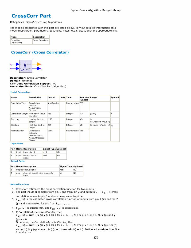
SystemVue - Algorithm Design Library
479
CrossCorr PartCategories: Signal Processing (algorithm)
The models associated with this part are listed below. To view detailed information on amodel (description, parameters, equations, notes, etc.), please click the appropriate link.
Model Description
CrossCorr(algorithm)
Cross Correlator
CrossCorr (Cross Correlator)
Description: Cross CorrelatorDomain: UntimedC++ Code Generation Support: NOAssociated Parts: CrossCorr Part (algorithm)
Model Parameters
Name Description Default Units Type RuntimeTunable
Range Symbol
CorrelationType Correlationmethod:NonCircular,Circular
NonCircular Enumeration YES
CorrelationLength Number of inputsamples
511 Integer NO [1:∞) N
StartLag Low lag limit tooutput
-255 Integer NO (-N:L<sub>h</sub>]
Ll
StopLag High lag limit tooutput
255 Integer NO [L<sub>l</sub>:N) Lh
Normalization Correlationestimatenormalization:None, UnBiased,Biased
None Enumeration YES
Input Ports
Port Name Description Signal Type Optional
1 input input signal real NO
2 input2 second inputsignal
real NO
Output Ports
Port Name Description Signal Type Optional
3 output output signal real NO
4 delay delay of input2 with respect toinput
int NO
Notes/Equations
CrossCorr estimates the cross correlation function for two inputs.1.The part inputs N samples from pin 1 and from pin 2 and outputs L l + L h + 1 cross2.
correlation values to pin 3 and one delay value to pin 4.r xy (k) is the estimated cross correlation function of inputs from pin 1 (x) and pin 23.
(y) and is evaluated for a k from L l, ... , L h.
r xy (L l) is output first, and r xy (L h) is output last.4.
If CorrelationType is NonCircular, then5.r xy (k) = sum { x (i) y (i + k) } for i = 1, ... , N. For p < 1 or p > N, x (p) and y
(p) are 0.Otherwise, the CorrelationType is Circular, thenr xy (k) = sum { x (i) y (i + k) } for i = 1, ... , N. For p < 1 or p > N, x (p) is x (q)
and y (p) is y (q) where q is ( (p − 1) modulo N) + 1 ). Define −1 modulo N as N −1, and so on.

SystemVue - Algorithm Design Library
480
Additionally, UnBiased and Biased autocorrelation estimates are supported.6.If CorrelationType is NonCircular, then for UnBiased Normalization, r xy (k) is
divided by N − | k |. For Biased Normalization, r xy (k) is divided by N.
If CorrelationType is Circular, then for UnBiased or Biased Normalization, r xy
(k) is divided by N.The estimated delay in samples of y with respect to x is output at pin 4. A negative7.value imply that x is delayed with respect to y.A typical application for CrossCorr is to find the best delay that will synchronize two8.signals. For this application set CorrelationType to NonCircular.
See:AutoCorr (algorithm)
References
A. V. Oppenheim and R. W. Schafer, Discrete-Time Signal Processing, Prentice-Hall:1.Englewood Cliffs, NJ, 1989.

SystemVue - Algorithm Design Library
481
CyclicShift PartCategories: Signal Processing (algorithm)
The models associated with this part are listed below. To view detailed information on amodel (description, parameters, equations, notes, etc.), please click the appropriate link.
Model Description
CyclicShift(algorithm)
Cyclically shift input data block with specified offset
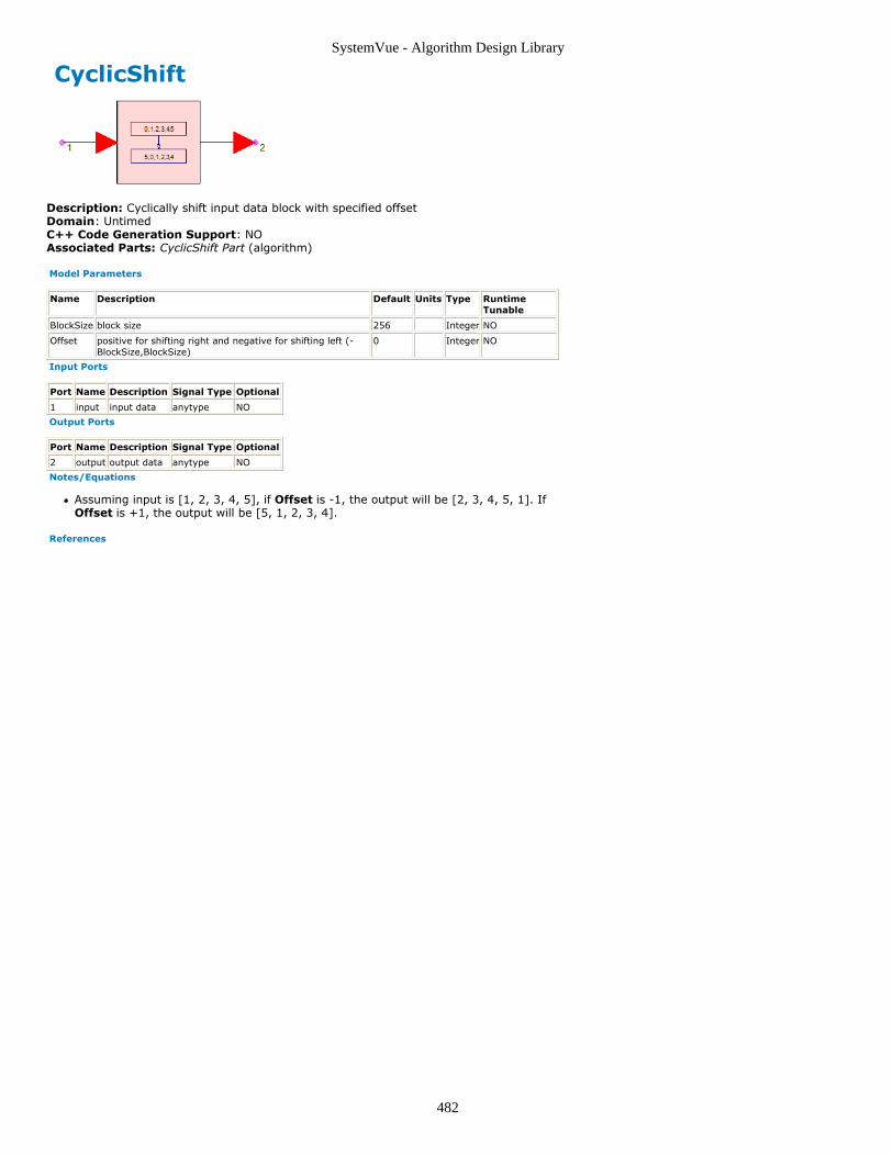
SystemVue - Algorithm Design Library
482
CyclicShift
Description: Cyclically shift input data block with specified offsetDomain: UntimedC++ Code Generation Support: NOAssociated Parts: CyclicShift Part (algorithm)
Model Parameters
Name Description Default Units Type RuntimeTunable
BlockSize block size 256 Integer NO
Offset positive for shifting right and negative for shifting left (-BlockSize,BlockSize)
0 Integer NO
Input Ports
Port Name Description Signal Type Optional
1 input input data anytype NO
Output Ports
Port Name Description Signal Type Optional
2 output output data anytype NO
Notes/Equations
Assuming input is [1, 2, 3, 4, 5], if Offset is -1, the output will be [2, 3, 4, 5, 1]. IfOffset is +1, the output will be [5, 1, 2, 3, 4].
References

SystemVue - Algorithm Design Library
483
DeadZone PartCategories: Signal Processing (algorithm)
The models associated with this part are listed below. To view detailed information on amodel (description, parameters, equations, notes, etc.), please click the appropriate link.
Model Description
DeadZone(algorithm)
Dead Zone Nonlinearity
DeadZone (Dead Zone Nonlinearity)
Description: Dead Zone NonlinearityDomain: UntimedC++ Code Generation Support: NOAssociated Parts: DeadZone Part (algorithm)
Model Parameters
Name Description Default Units Type Runtime Tunable Range
K Magnitude gain 1 Float YES (-∞:0.0) or (0.0:∞)
Low Lower dead zone value 0 Float YES (-∞:High)
High Higher dead zone value 1 Float YES (-∞:∞)
Input Ports
Port Name Description Signal Type Optional
1 input input signal real NO
Output Ports
Port Name Description Signal Type Optional
2 output output signal real NO
Notes/Equations
The dead zone nonlinearity is defined as follows:1.
where:x(n) is input for sample nK is the K parameterV h is the High parameter
V l is the Low parameter
y(n) is output for sample nFor every input, there is one output.2.Shown below is the input/output characteristic of DeadZone with K = 1, Low = 0 and3.High = 1.
DeadZone Signal Plot

SystemVue - Algorithm Design Library
484
Delay Part
Ideal Time Delay Block (DELAY). Delays the signal for a certain amount of time.
The models and symbols associated with this part are listed below. To view detailedinformation on a model (description, parameters, equations, notes, etc.), please select theappropriate link.
For a list of available parts organized by Schematic Toolbar, please see Appendix C - Toolbars(users).
Model
Delay(algorithm)
Symbol
DELAY
For a list of available symbols see the Symbol Reference .
Delay (Delay)
Description: DelayDomain: UntimedC++ Code Generation Support: NOAssociated Parts: Delay Part (algorithm)
Model Parameters
Name Description Default Units Type RuntimeTunable
Range
N Sample delay size 1 Integer NO [0:∞)
OutputTiming Output start time: EqualToInput,BeforeInput
EqualToInput Enumeration NO
Input Ports
Port Name Signal Type Optional
1 input anytype NO
Output Ports
Port Name Signal Type Optional
2 output anytype NO
Notes/Equations
The Delay model introduces a delay of N samples to the input signal.1.For every input, there is one output.2.The initial N output samples have a null value. For scalar signals, a null value is 0.3.For matrix signals, a null value is a matrix with the same size as the input matrix andwith all its elements set to 0.
See:InitDelay (algorithm)
InitDelay (Delay with Initial Value)
Description: Delay with Initial ValueDomain: UntimedC++ Code Generation Support: YES (see Note)Associated Parts: Delay Part (algorithm)
Model Parameters

SystemVue - Algorithm Design Library
485
Name Description Default Units Type Runtime Tunable Range
N Sample delaysize
1 Integer NO [0:∞)
InitialDelay Initial data value None NO
Input Ports
Port Name Signal Type Optional
1 input anytype NO
Output Ports
Port Name Signal Type Optional
2 output anytype NO
NoteThis model does not support C++ code generation if the port type is resolved to envelope signal (sim) orvariant (sim).
Notes/Equations
InitDelay delays input tokens from output by N sets of initial delay tokens.1.For every input, there is an output value.2.
See:Delay (algorithm)

SystemVue - Algorithm Design Library
486
DTFT PartCategories: Signal Processing (algorithm)
The models associated with this part are listed below. To view detailed information on amodel (description, parameters, equations, notes, etc.), please click the appropriate link.
Model Description
DTFT(algorithm)
Discrete-Time Fourier Transform
DTFT (Discrete-Time Fourier Transform)
Description: Discrete-Time Fourier TransformDomain: UntimedC++ Code Generation Support: NOAssociated Parts: DTFT Part (algorithm)
Model Parameters
Name Description Default Units Type RuntimeTunable
Range Symbol
Length Length of input signal 8 Integer NO (0:∞) L
NumberOfSamples Number of transform samplesto output
128 Integer NO (0:∞) N
TimeBetweenSamples Time between input samples 1 Float YES (0:∞) T
Input Ports
Port Name Description Signal Type Optional
1 signal signal to be transformed complex NO
2 omega frequency values at which to compute the transform real NO
Output Ports
Port Name Description Signal Type Optional
3 dtft transform values complex NO
Notes/Equations
The DTFT model calculates the Discrete-Time Fourier transform (DTFT) of the1.sequence applied at its signal input at each of the frequency points specified on theomega input.At every execution of this model, L samples are read from its signal input, N samples2.are read from its omega input, and N samples written to its output.The DTFT of a sequence x[n] is a continuous function of ω defined by3.
If the sequence x[n] is obtained by sampling a continuous time signal x c (t) at
intervals of T, that is x[n] = x c (nT), and if X c (f), the continuous-time Fourier
Transform of x c (t), equals 0 for f > 1/(2T), then X(jω) and X c (f) have the following
relationship:
, for f < 1 / (2T).The DTFT model can calculate X(jω) at arbitrary values of ω for sequences x[n] of4.finite length. Let the L values on the signal input be x[0], x[1], ... , x[L − 1] and theN values on the omega input be ω[0], ω[1], ... , ω[N − 1]. Then the N values at theoutput are:
, i = 0, 1, ... , N − 1.

SystemVue - Algorithm Design Library
487
Notice that in this last formula the exponent of e has the extra term T compared tothe formula defining the DTFT. Therefore, to calculate the Fourier transform of thecorresponding continuous time signal x c (t) at the frequencies f i , i = 0, 1, ... , N,
generate the values ω i = 2πf i, apply them at the omega input, and scale the output
by T. The values f i do not need to span the entire frequency range of the signal or
be equally spaced.
See:FFT_Cx (algorithm)
References
A. V. Oppenheim and R. W. Schafer, Discrete-Time Signal Processing, Prentice-Hall:1.Englewood Cliffs, NJ, 1989.

SystemVue - Algorithm Design Library
488
Expand PartCategories: Signal Processing (algorithm)
The models associated with this part are listed below. To view detailed information on amodel (description, parameters, equations, notes, etc.), please click the appropriate link.
Model Description
Expand(algorithm)
Expander Part of a Compander
Expand (Expander Part of a Compander)
Description: Expander Part of a CompanderDomain: UntimedC++ Code Generation Support: NOAssociated Parts: Expand Part (algorithm)
Model Parameters
Name Description Default Units Type Runtime Tunable Range
CompressionType Compression law: MU-law, A-law
MU-law Enumeration YES
CompressionK Compression constant 1 Float YES
Max Maximum input value magnitude 1 Float YES (0.0:∞)
Input Ports
Port Name Signal Type Optional
1 input real NO
Output Ports
Port Name Signal Type Optional
2 output real NO
Notes/Equations
Expand performs A-law or MU-law expansion.1.For every input, there is an output value.2.Let3.
thenMU-law:
A-law:
where:x(n) is input for sample nV M is Max
y(n) is output for sample nµ is CompressionK for MU-LawA is CompressionK for A-LawShown below is the input/output characteristic of Expand with Type = MU-law,4.CompressionK = 255 and Max = 1V.
Expand Component Signal Plot

SystemVue - Algorithm Design Library
489
See:Compress (algorithm)

SystemVue - Algorithm Design Library
490
FFT_Cx PartCategories: C++ Code Generation (algorithm), Signal Processing (algorithm)
The models associated with this part are listed below. To view detailed information on amodel (description, parameters, equations, notes, etc.), please click the appropriate link.
Model Description
FFT_Cx(algorithm)
Complex Fast Fourier Transform
FFT_Cx (Complex Fast Fourier Transform)
Description: Complex Fast Fourier TransformDomain: UntimedC++ Code Generation Support: YESAssociated Parts: FFT Cx Part (algorithm)
Model Parameters
Name Description Default Units Type RuntimeTunable
FFTSize Output transform size 256 Integer NO
Size Number of input samples to read 256 Integer NO
Direction Direction of transform: Inverse, Forward Forward Enumeration NO
FreqSequence Sequence for the frequency terms: 0-pos-neg,neg-0-pos
0-pos-neg
Enumeration NO
Input Ports
Port Name Signal Type Optional
1 input complex NO
Output Ports
Port Name Signal Type Optional
2 output complex NO
Notes/Equations
The FFT_Cx model computes the DFT (Discrete Fourier Transform) of the input signal1.using a mixed radix FFT (Fast Fourier Transform) algorithm.At every execution of this model, Size complex samples are read from the input. This2.block of Size samples is zero padded (if Size < FFTSize) to create a block of FFTSizesamples. The block of FFTSize samples is then processed by a mixed radix FFTalgorithm to produce FFT_Size equally spaced samples that is the DFT of the inputsignal.The Direction parameter specifies whether a forward or inverse FFT will be3.performed.The FreqSequence parameter specifies the order in which the frequency values are4.written to the output (forward FFT case) or read from the input (inverse FFT case).
See:DTFT (algorithm)
References
A. V. Oppenheim and R. W. Schafer, Discrete-Time Signal Processing, Prentice-Hall:1.Englewood Cliffs, NJ, 1989.

SystemVue - Algorithm Design Library
491
FFT_Shift PartCategories: Signal Processing (algorithm)
The models associated with this part are listed below. To view detailed information on amodel (description, parameters, equations, notes, etc.), please click the appropriate link.
Model Description
FFT_Shift(algorithm)
swaps the left halves and right halves of outputs of fft or inputs of ifft

SystemVue - Algorithm Design Library
492
FFT_Shift
Description: swaps the left halves and right halves of outputs of fft or inputs of ifftDomain: UntimedC++ Code Generation Support: NOAssociated Parts: FFT SHift Part (algorithm)
Model Parameters
Name Description Default Units Type Runtime Tunable
FFTSize FFT or IFFT size 256 Integer NO
Direction FFT shift or IFFT shift: FFTShift, IFFTShift FFTShift Enumeration NO
Input Ports
Port Name Description Signal Type Optional
1 input input data anytype NO
Output Ports
Port Name Description Signal Type Optional
2 output output data anytype NO
Notes/Equations
This model shifts zero-frequency component to center of the spectrum in FFT/IFFToperation.
If FFTSize is 6 (even), the spectrum with zero-frequency component in center is [-3,-2, -1, 0, 1, 2], the output of FFT (or input of IFFT) should be [0, 1, 2, -3, -2, -1].If FFTSize is 5 (even), the spectrum with zero-frequency component in center is [-2,-1, 0, 1, 2], the output of FFT (or input of IFFT) should be [0, 1, 2, -2, -1].This model should connect output of FFT model (Direction=FFTShift) or input of IFFTmodel (Direction=IFFTShift).
References

SystemVue - Algorithm Design Library
493
GeometricMean PartCategories: Signal Processing (algorithm)
The models associated with this part are listed below. To view detailed information on amodel (description, parameters, equations, notes, etc.), please click the appropriate link.
Model Description
GeometricMean(algorithm)
Geometric Mean Function
GeometricMean (Geometric Mean Function)
Description: Geometric Mean FunctionDomain: UntimedC++ Code Generation Support: NOAssociated Parts: GeometricMean Part (algorithm)
Model Parameters
Name Description Default Units Type Runtime Tunable Range
N Number of samples in a block 10 Integer NO [1:∞)
Gain Gain value 1 Float YES (-∞:∞)
Input Ports
Port Name Signal Type Optional
1 input real NO
Output Ports
Port Name Signal Type Optional
2 output real NO
Notes/EquationsThe GeometricMean model computes the geometric mean for every block of N input1.samples.
At every execution of this model, N samples are read from the input and 1 sample is2.written to the output.
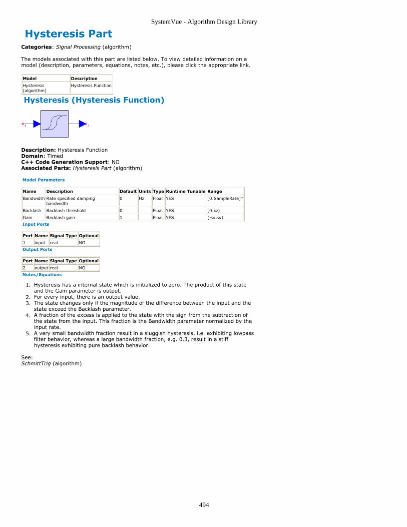
SystemVue - Algorithm Design Library
494
Hysteresis PartCategories: Signal Processing (algorithm)
The models associated with this part are listed below. To view detailed information on amodel (description, parameters, equations, notes, etc.), please click the appropriate link.
Model Description
Hysteresis(algorithm)
Hysteresis Function
Hysteresis (Hysteresis Function)
Description: Hysteresis FunctionDomain: TimedC++ Code Generation Support: NOAssociated Parts: Hysteresis Part (algorithm)
Model Parameters
Name Description Default Units Type Runtime Tunable Range
Bandwidth Rate specified dampingbandwidth
0 Hz Float YES [0:SampleRate]†
Backlash Backlash threshold 0 Float YES [0:∞)
Gain Backlash gain 1 Float YES (-∞:∞)
Input Ports
Port Name Signal Type Optional
1 input real NO
Output Ports
Port Name Signal Type Optional
2 output real NO
Notes/Equations
Hysteresis has a internal state which is initialized to zero. The product of this state1.and the Gain parameter is output.For every input, there is an output value.2.The state changes only if the magnitude of the difference between the input and the3.state exceed the Backlash parameter.A fraction of the excess is applied to the state with the sign from the subtraction of4.the state from the input. This fraction is the Bandwidth parameter normalized by theinput rate.A very small bandwidth fraction result in a sluggish hysteresis, i.e. exhibiting lowpass5.filter behavior, whereas a large bandwidth fraction, e.g. 0.3, result in a stiffhysteresis exhibiting pure backlash behavior.
See:SchmittTrig (algorithm)

SystemVue - Algorithm Design Library
495
Limit PartCategories: Signal Processing (algorithm)
The models associated with this part are listed below. To view detailed information on amodel (description, parameters, equations, notes, etc.), please click the appropriate link.
Model Description
Limit(algorithm)
Limiter
Limit (Limiter)
Description: LimiterDomain: UntimedC++ Code Generation Support: NOAssociated Parts: Limit Part (algorithm)
Model Parameters
Name Description Default Units Type RuntimeTunable
Range
K Magnitude gain 1 Float YES (-∞:0.0) or(0.0:∞)
Bottom Lower output saturation value 0 Float YES (-∞:Top)
Top Higher output saturation value 1 Float YES (-∞:∞)
LimiterType Type of limiting curve: linear,atan
linear Enumeration YES
Input Ports
Port Name Signal Type Optional
1 input real NO
Output Ports
Port Name Signal Type Optional
2 output real NO
Notes/Equations
Limit models two different types of limiting nonlinearities.1.For every input, there is an output value.2.If linear:3.
If atan:
where:x(n) is input for sample nV l is the Bottom parameter
V h is the Top parameter
K is the K parametery(n) is output for sample nShown below are input/output characteristics of Limit with parameters K = 1, Bottom4.= −1, and Top = 1 for linear and atan types.

SystemVue - Algorithm Design Library
496
Limit Component Signal Plot

SystemVue - Algorithm Design Library
497
LinearQuantizer PartCategories: Signal Processing (algorithm)
The models associated with this part are listed below. To view detailed information on amodel (description, parameters, equations, notes, etc.), please click the appropriate link.
Model Description
LinearQuantizer(algorithm)
Uniform Quantizer with Step Number Output
LinearQuantizer (Uniform Quantizer with StepNumber Output)
Description: Uniform Quantizer with Step Number OutputDomain: UntimedC++ Code Generation Support: NOAssociated Parts: LinearQuantizer Part (algorithm)
Model Parameters
Name Description Default Units Type Runtime Tunable Range
Levels Number of quantizationlevels
128 Integer YES [2:∞)
Low Lowest quantization level -3 Float YES (-∞:High)
High Highest quantization level 3 Float YES (-∞:∞)
Input Ports
Port Name Description Signal Type Optional
1 input input signal real NO
Output Ports
Port Name Description Signal Type Optional
2 amplitude quantized signal real NO
3 stepNumber quantization level index int NO
Notes/Equations
The input signal is quantized to the number of levels given by the Levels parameter.1.For every input, there is an output at both output ports.2.Quantization levels start at Low, end at High, and are uniformly spaced in between.3.Input is mapped to the closest quantization level.4.Quantized input is output to the amplitude port. Its quantization level index is output5.to the stepNumber port as an integer from 0 (corresponding to the quantization levelof Low) to Levels - 1 (corresponding to the quantization level of High).
See:AdaptLinQuant (algorithm)Quantizer (algorithm)Quantizer2D (algorithm)
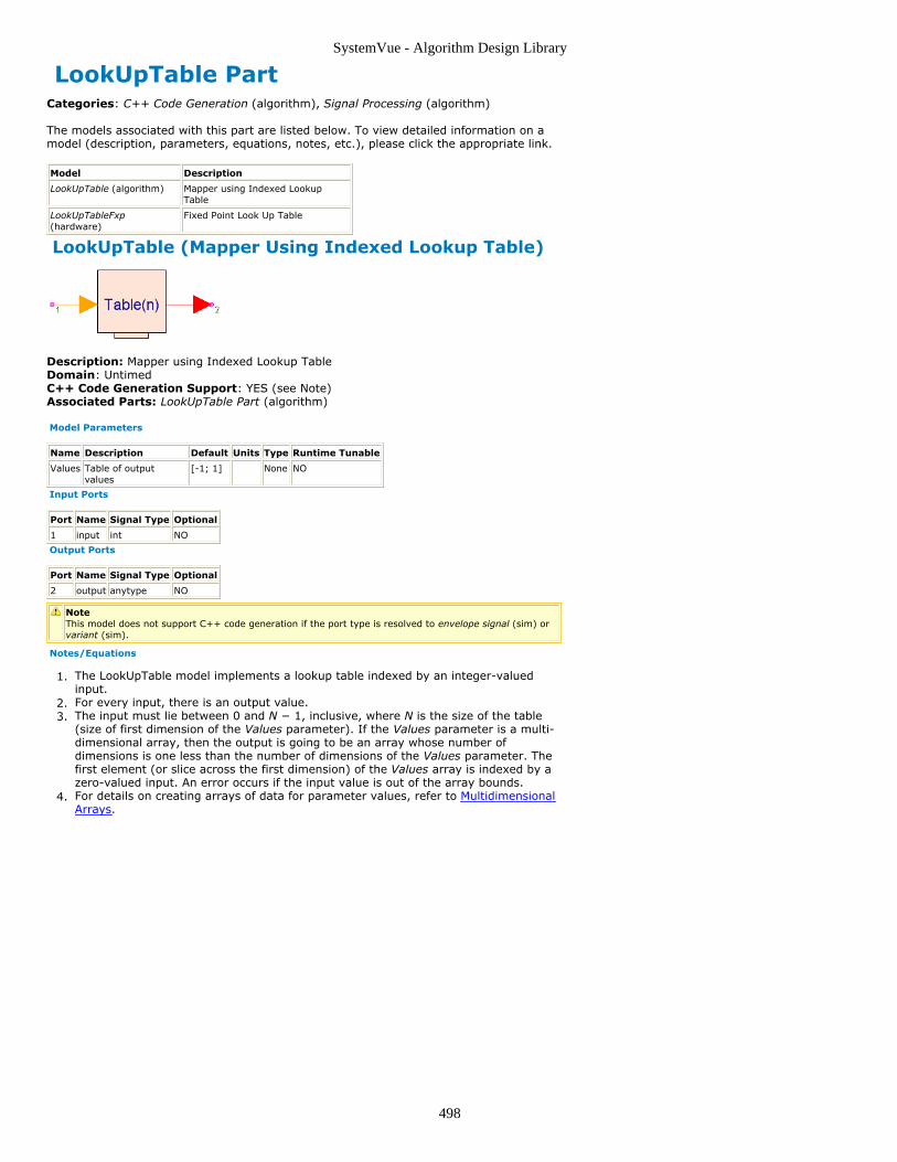
SystemVue - Algorithm Design Library
498
LookUpTable PartCategories: C++ Code Generation (algorithm), Signal Processing (algorithm)
The models associated with this part are listed below. To view detailed information on amodel (description, parameters, equations, notes, etc.), please click the appropriate link.
Model Description
LookUpTable (algorithm) Mapper using Indexed LookupTable
LookUpTableFxp(hardware)
Fixed Point Look Up Table
LookUpTable (Mapper Using Indexed Lookup Table)
Description: Mapper using Indexed Lookup TableDomain: UntimedC++ Code Generation Support: YES (see Note)Associated Parts: LookUpTable Part (algorithm)
Model Parameters
Name Description Default Units Type Runtime Tunable
Values Table of outputvalues
[-1; 1] None NO
Input Ports
Port Name Signal Type Optional
1 input int NO
Output Ports
Port Name Signal Type Optional
2 output anytype NO
NoteThis model does not support C++ code generation if the port type is resolved to envelope signal (sim) orvariant (sim).
Notes/Equations
The LookUpTable model implements a lookup table indexed by an integer-valued1.input.For every input, there is an output value.2.The input must lie between 0 and N − 1, inclusive, where N is the size of the table3.(size of first dimension of the Values parameter). If the Values parameter is a multi-dimensional array, then the output is going to be an array whose number ofdimensions is one less than the number of dimensions of the Values parameter. Thefirst element (or slice across the first dimension) of the Values array is indexed by azero-valued input. An error occurs if the input value is out of the array bounds.For details on creating arrays of data for parameter values, refer to Multidimensional4.Arrays.

SystemVue - Algorithm Design Library
499
MaxMin PartCategories: Signal Processing (algorithm)
The models associated with this part are listed below. To view detailed information on amodel (description, parameters, equations, notes, etc.), please click the appropriate link.
Model Description
MaxMin(algorithm)
Maximum or Minimum ValueFunction
MaxMin (Maximum or Minimum Value Function)
Description: Maximum or Minimum Value FunctionDomain: UntimedC++ Code Generation Support: NOAssociated Parts: MaxMin Part (algorithm)
Model Parameters
Name Description Default Units Type RuntimeTunable
Range
N Number of samples 10 Integer NO [0:∞)
MaxOrMin Output value: min, max max Enumeration YES
Compare Compare input value or magnitude:valueIn, magnitudeIn
valueIn Enumeration YES
OutputType Output value or magnitude: valueOut,magnitudeOut
valueOut Enumeration YES
Input Ports
Port Name Signal Type Optional
1 input real NO
Output Ports
Port Name Signal Type Optional
2 output real NO
3 index int NO
Notes/Equations
MaxMin finds the minimum or minimum value or magnitude of N input values.1.For every N input values, one value is output.2.If Compare = valueIn, the input with the maximum or minimum value is located,3.otherwise the input with the maximum or minimum magnitude is located.If OutputType = magnitudeOut, the magnitude of the result is output, otherwise the4.result is output.The default parameters output the maximum value among N=10 input samples. The5.index of the maximum is output to the index port where 0 locates the first inputvalue.Use MaxMin to operate over multiple data streams by preceding it with a Commutator6.and setting the N parameter appropriately.

SystemVue - Algorithm Design Library
500
PattMatch PartCategories: Signal Processing (algorithm)
The models associated with this part are listed below. To view detailed information on amodel (description, parameters, equations, notes, etc.), please click the appropriate link.
Model Description
PattMatch(algorithm)
Pattern Cross Correlator usingTemplate
PattMatch (Pattern Cross Correlator using Template)
Description: Pattern Cross Correlator using TemplateDomain: UntimedC++ Code Generation Support: NOAssociated Parts: PattMatch Part (algorithm)
Model Parameters
Name Description Default Units Type Runtime Tunable Range
TempSize Number of samples in template 32 Integer NO (0:∞)
WinSize Number of samples in search template 176 Integer NO [TempSize:∞)
Input Ports
Port Name Description Signal Type Optional
1 templ templateinput
real NO
2 window window input real NO
Output Ports
Port Name Description Signal Type Optional
3 index index output int NO
4 values cross-correlation output real NO
Notes/Equations
The PattMatch model accepts a template and a search window and tries to find the1.position in the search window where the template matches best.At every execution of this model, TempSize samples are read from the templ input2.and WinSize samples are read from the window input. At the same time, one sampleis written to the index output and (WinSize − TempSize + 1) samples are written tothe values output.The algorithm for finding the best template match position starts by placing the3.template at the left end of the window (first samples of template and window arealigned) and calculating the cross-correlation between them. Then the template isshifted across the window one sample at a time and the cross-correlation iscomputed at each step until the template reaches the right end of the window (lastsamples of template and window are aligned). The cross-correlation values areoutput on the values output. The index output is the value of the shift (in number ofsamples) that gives the largest cross-correlation.The cross-correlation values are normalized against the energy of the window under4.the template:
where T is the template, W is the window, n is the index value, and T size equals
TempSize.Note that if the template is identical to a certain segment of the window, then thecross-correlation value C(n) for that segment will be 1.0. Therefore, the index with

SystemVue - Algorithm Design Library
501
the highest cross-correlation value may not be the best match if that value is greaterthan 1.0.

SystemVue - Algorithm Design Library
502
PcwzLinear PartCategories: Signal Processing (algorithm)
The models associated with this part are listed below. To view detailed information on amodel (description, parameters, equations, notes, etc.), please click the appropriate link.
Model Description
PcwzLinear(algorithm)
Piecewise LinearMapper
PcwzLinear (Piecewise Linear Mapper)
Description: Piecewise Linear MapperDomain: UntimedC++ Code Generation Support: NOAssociated Parts: PcwzLinear Part (algorithm)
Model Parameters
Name Description Default Units Type Runtime Tunable
Breakpoints Endpoints and breakpoints in the mapping [-1-j, j, 1-j] Complexarray
NO
Input Ports
Port Name Description Signal Type Optional
1 input input signal real NO
Output Ports
Port Name Description Signal Type Optional
2 output output signal real NO
Notes/Equations
PcwzLinear implements a piecewise linear mapping from the input to the output.1.For every input, there is one output value.2.Mapping is given by a sequence of (x,y) pairs that specify breakpoints in the function.3.The (x,y) pairs are expressed in the Breakpoints parameter in the complex form, i.e.x+jy. The sequence of x values must be increasing.The function implemented by PcwzLinear can be represented by drawing straight4.lines between the (x,y) pairs in sequence. Additionally, the first breakpoint isextended to x=−∞, and the last breakpoint is extended to x=+∞. Each input istreated as a point on the x axis, and the corresponding y value is output.For example, the default mapping is the tent map. Inputs between −1.0 and 0.0 are5.linearly mapped into the range −1.0 to 1.0. Inputs between 0.0 and 1.0 are mappedinto the same range, but with opposite slope, 1.0 to −1.0. If the input is −2.0, theoutput will be −1.0. If the input is +2.0, the output will again be −1.0.

SystemVue - Algorithm Design Library
503
Quantizer2D PartCategories: Signal Processing (algorithm)
The models associated with this part are listed below. To view detailed information on amodel (description, parameters, equations, notes, etc.), please click the appropriate link.
Model Description
Quantizer2D(algorithm)
2-Dimensional Quantizer using Threshold List
Quantizer2D (2-Dimensional Quantizer usingThreshold List)
Description: 2-Dimensional Quantizer using Threshold ListDomain: UntimedC++ Code Generation Support: NOAssociated Parts: Quantizer2D Part (algorithm)
Model Parameters
Name Description Default Units Type Runtime Tunable Range
VxMax Maximum real output level 1 Float YES (-∞:∞)
VxMin Minimum real output level -1 Float YES (-∞:VxMax)
Nx Number of real output levels 16 Integer YES [1:∞)
VyMax Maximum imaginary output level 1 Float YES (-∞:∞)
VyMin Minimum imaginary output level -1 Float YES (-∞:VyMax)
Ny Number of imaginary output levels 16 Integer YES [1:∞)
QuantList User-defined quantization points Complexarray
NO
Input Ports
Port Name Signal Type Optional
1 input complex NO
Output Ports
Port Name Signal Type Optional
2 output complex NO
Notes/Equations
The complex number input is mapped to one of a finite set of complex numbers.1.For every input, one value is output.2.An arbitrary set of output points can be specified with the QuantList parameter.3.Otherwise, the parameters VxMax, VxMin, Nx, VyMax, VyMin and Ny can be used tocreate a rectangular grid of output points.Each input is mapped to the nearest output point, where the metric used to4.determine the nearest output point is the Euclidean distance. This type of a quantizeris also referred to as a Voronoi or a nearest neighbor vector quantizer.2D Quantizer with Three Output Points shows an example where three output points5.P1, P2, and P3 have been specified. The entire 2D plane is then divided into 3regions, R1, R2, and R3, which are shown by the dotted lines. Any input point inregion R1 is mapped to the output point P1 (and similarly for the other regions).2D Quantizer with Output Points On a Grid illustrates how a rectangular grid of6.output points can be created by using the parameters VxMax, VxMin, Nx, VyMax,VyMin and Ny.Due to the regular lattice structure of this quantizer, it can be implemented efficientlyin terms of speed. Therefore, it is more efficient to use this second method ofspecifying a quantizer than using a list of output points.When a list is used to specify output points, data is entered for the QuantList7.parameter as array of complex values. Data entered as an explicit array has theform:QuantList = [1, 0.707+0.707j, j, −0.707+0.707j, −1, −0.707−0.707j, −j,0.707−0.707j]The above list can be used to create a quantizer for an 8PSK receiver whose signal

SystemVue - Algorithm Design Library
504
set consists of 8 points equally spaced on a unit circle. Quantizer2D shows the pointsand the decision regions (in dotted lines) for this quantizer.
See:AdaptLinQuant (algorithm)LinearQuantizer (algorithm)Quantizer (algorithm)
2D Quantizer with Three Output Points
2D Quantizer with Output Points On a Grid
Quantizer2D

SystemVue - Algorithm Design Library
505
Quantizer PartCategories: Signal Processing (algorithm)
The models associated with this part are listed below. To view detailed information on amodel (description, parameters, equations, notes, etc.), please click the appropriate link.
Model Description
Quantizer(algorithm)
Quantizer using Threshold List
Quantizer (Quantizer using Threshold List)
Description: Quantizer using Threshold ListDomain: UntimedC++ Code Generation Support: NOAssociated Parts: Quantizer Part (algorithm)
Model Parameters
Name Description Default Units Type Runtime Tunable
Thresholds Quantization thresholds (increasing order) [0] Floating point array NO
Levels Output levels (if empty use 0, 1, 2, ...) Floating point array NO
Input Ports
Port Name Description Signal Type Optional
1 input real NO
Output Ports
Port Name Description Signal Type Optional
2 output real NO
3 stepNumber Level number of the quantization from 0 to N int NO
Notes/Equations
Quantize the input to one of N+1 possible output levels found in the Levels1.parameter using N thresholds from the Thresholds parameter.For every input, one sample is output to both output ports.2.Thresholds must be ordered in ascending value.3.For an input less than or equal to the n-th threshold, but larger than all previous4.thresholds, Levels[n] is output, and the value n−1 is output to the stepNumber port.If the input is less or equal to the first threshold, then output is the first level,5.Levels[1]. If the input is greater than all thresholds, output is Levels[N+1].If Levels is specified, there must be one more level than thresholds. The default for6.Levels is 0, 1, 2, ... N.Quantizer takes on the order of log N iterations to find the correct level.7.
See:AdaptLinQuant (algorithm)LinearQuantizer (algorithm)Quantizer2D (algorithm)

SystemVue - Algorithm Design Library
506
Reverse PartCategories: Signal Processing (algorithm)
The models associated with this part are listed below. To view detailed information on amodel (description, parameters, equations, notes, etc.), please click the appropriate link.
Model Description
reverse(algorithm)
Data Reverser
reverse
Description: Data ReverserDomain: UntimedC++ Code Generation Support: NOAssociated Parts: Reverse Part (algorithm)
Model Parameters
Name Description Default Units Type Runtime Tunable Range
N Number of data items read andwritten
64 Integer NO [1:∞)
Input Ports
Port Name Signal Type Optional
1 input anytype NO
Output Ports
Port Name Signal Type Optional
2 output anytype NO
Notes/Equations
A block of N samples is input, and that block of N samples is output in the reverse1.input order.

SystemVue - Algorithm Design Library
507
SchmittTrig PartCategories: Signal Processing (algorithm)
The models associated with this part are listed below. To view detailed information on amodel (description, parameters, equations, notes, etc.), please click the appropriate link.
Model Description
SchmittTrig(algorithm)
Schmitt Trigger
SchmittTrig (Schmitt Trigger)
Description: Schmitt TriggerDomain: UntimedC++ Code Generation Support: NOAssociated Parts: SchmittTrig Part (algorithm)
Model Parameters
Name Description Default Units Type Runtime Tunable Range
ILow Lower input trigger value -1 Float YES (-∞:IHigh)
IHigh Higher input trigger value 1 Float YES (-∞:∞)
OLow Lower output trigger value -1 Float YES (-∞:OHigh)
OHigh Higher output trigger value 1 Float YES (-∞:∞)
Input Ports
Port Name Signal Type Optional
1 input real NO
Output Ports
Port Name Signal Type Optional
2 output real NO
Notes/Equations
SchmittTrig is a Schmitt trigger with programmable levels.1.For every input, one value is output.2.The output signal versus input signal plot, with parameters ILow = −1, IHigh = 1,3.OLow = −1, and OHigh = 1, is shown below.
See:Hysteresis (algorithm)
SchmittTrig Signal Plot

SystemVue - Algorithm Design Library
508
SlidWinAvg PartCategories: Signal Processing (algorithm)
The models associated with this part are listed below. To view detailed information on amodel (description, parameters, equations, notes, etc.), please click the appropriate link.
Model Description
SlidWinAvg(algorithm)
Sliding-WindowAverager
SlidWinAvg (Sliding-Window Averager)
Description: Sliding-Window AveragerDomain: UntimedC++ Code Generation Support: NOAssociated Parts: SlidWinAvg Part (algorithm)
Model Parameters
Name Description Default Units Type Runtime Tunable Range
WindowSize Size of sliding window 3 Integer NO (1:∞)
Input Ports
Port Name Description Signal Type Optional
1 input input signal real NO
Output Ports
Port Name Description Signal Type Optional
2 output output signal real NO
Notes/Equations
The average of the sample values captured in the most recent window of inputs is1.output.For every input, an averaged value is output.2.Samples before the first are zero valued.3.
See:Integrator (algorithm)IntegratorCx (algorithm)IntegratorInt (algorithm)
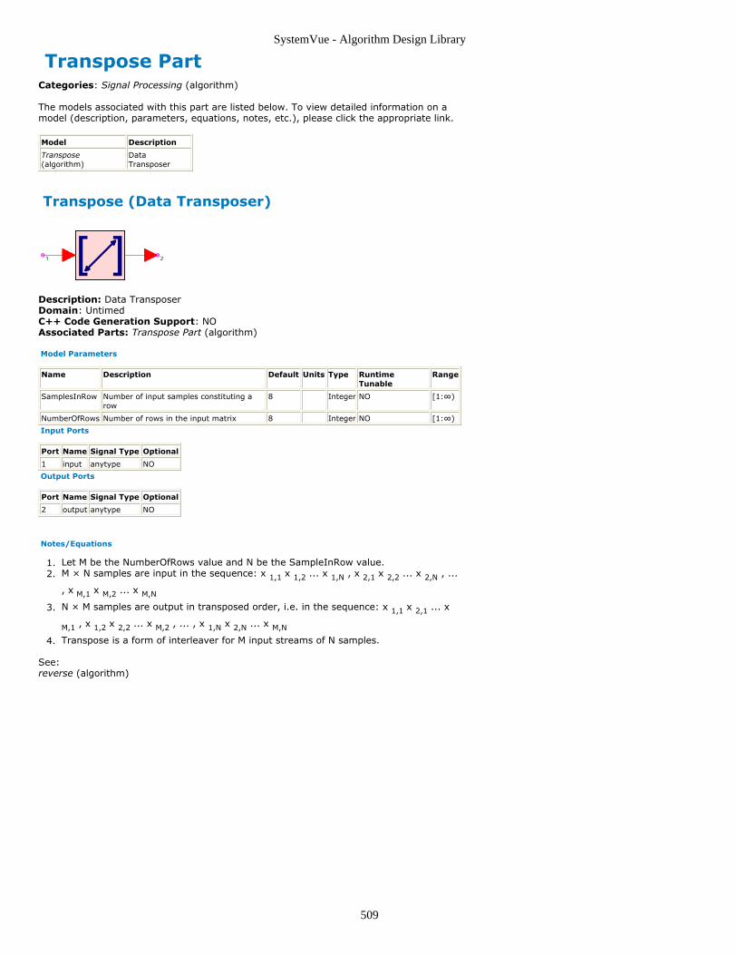
SystemVue - Algorithm Design Library
509
Transpose PartCategories: Signal Processing (algorithm)
The models associated with this part are listed below. To view detailed information on amodel (description, parameters, equations, notes, etc.), please click the appropriate link.
Model Description
Transpose(algorithm)
DataTransposer
Transpose (Data Transposer)
Description: Data TransposerDomain: UntimedC++ Code Generation Support: NOAssociated Parts: Transpose Part (algorithm)
Model Parameters
Name Description Default Units Type RuntimeTunable
Range
SamplesInRow Number of input samples constituting arow
8 Integer NO [1:∞)
NumberOfRows Number of rows in the input matrix 8 Integer NO [1:∞)
Input Ports
Port Name Signal Type Optional
1 input anytype NO
Output Ports
Port Name Signal Type Optional
2 output anytype NO
Notes/Equations
Let M be the NumberOfRows value and N be the SampleInRow value.1.M × N samples are input in the sequence: x 1,1 x 1,2 ... x 1,N , x 2,1 x 2,2 ... x 2,N , ...2.
, x M,1 x M,2 ... x M,N
N × M samples are output in transposed order, i.e. in the sequence: x 1,1 x 2,1 ... x3.
M,1 , x 1,2 x 2,2 ... x M,2 , ... , x 1,N x 2,N ... x M,N
Transpose is a form of interleaver for M input streams of N samples.4.
See:reverse (algorithm)

SystemVue - Algorithm Design Library
510
VarDelay PartCategories: C++ Code Generation (algorithm), Signal Processing (algorithm)
The models associated with this part are listed below. To view detailed information on amodel (description, parameters, equations, notes, etc.), please click the appropriate link.
Model Description
VarDelay(algorithm)
Variable Delay
VarDelay (Variable Delay)
Description: Variable DelayDomain: UntimedC++ Code Generation Support: YES (see Note)Associated Parts: VarDelay Part (algorithm)
Model Parameters
Name Description Default Units Type Runtime Tunable Range
MaxDelay Maximumdelay
10 Integer NO [0:∞)
Input Ports
Port Name Signal Type Optional
1 input anytype NO
2 control int YES
Output Ports
Port Name Signal Type Optional
3 output anytype NO
NoteThis model does not support C++ code generation if the port type is resolved to envelope signal (sim) orvariant (sim).
Notes/Equations
VarDelay introduces a varying delay to the input signal.1.This model reads 1 sample from the input and writes 1 sample to the output.2.The delay in samples is controlled by the signal applied to the control port.3.MaxDelay specifies the maximum control input. A buffer of MaxDelay samples is used4.to store the most recent samples and is initialized with zero values.The control input determines which sample in the buffer is output. A control value of5.0 or less outputs the most recent input. A control value of MaxDelay or greateroutputs the oldest sample in the buffer. A control value of N where 0 < N < MaxDelayoutputs the sample from the buffer that was read N executions back.This model can be used with the CrossCorr (algorithm) model to synchronize signals.6.

SystemVue - Algorithm Design Library
511
Variance PartCategories: Signal Processing (algorithm)
The models associated with this part are listed below. To view detailed information on amodel (description, parameters, equations, notes, etc.), please click the appropriate link.
Model Description
Variance(algorithm)
Variance Function
Variance (Variance Function)
Description: Variance FunctionDomain: UntimedC++ Code Generation Support: NOAssociated Parts: Variance Part (algorithm)
Model Parameters
Name Description Default Units Type RuntimeTunable
Range
BlockSize Number of inputs to process between each meanand variance estimate
1 Integer NO [1:∞)
Input Ports
Port Name Signal Type Optional
1 in real NO
Output Ports
Port Name Signal Type Optional
2 mean real NO
3 variance real NO
Notes/Equations
The Variance model calculates a running estimate of the mean and variance of the1.input signal. These estimates are reported every BlockSize input samples.At every execution of this model, BlockSize samples are read from the input and one2.sample is written to the mean and variance outputs.The mean and variance values written to the mean and variance outputs respectively3.are not the mean and variance of the last block of BlockSize samples. They are themean and variance of all samples read from the beginning of the simulation.

SystemVue - Algorithm Design Library
512
SinksThe Sinks library provides parts that can record and/or post-process (performmeasurements on) the input they receive. Several commonly used measurements areprovided, such as spectrum analysis, EVM, CCDF, BER, etc.
For more information see About Sinks (algorithm).
ContentsBER FER Part (algorithm)BER IS Part (algorithm)CCDF Part (algorithm)DataPort Part (algorithm)EVM Part (algorithm)FlexDCA Sink Part (algorithm)RMSE Part (algorithm)Sink Part (algorithm)SpectrumAnalyzer Part (algorithm)WriteBaseBandStudioFile Part (algorithm)WriteFile Part (algorithm)

SystemVue - Algorithm Design Library
513
About Sinks Access to Envelope Signal CharacterizationFrequency in a DatasetWhen an envelope signal with characterization frequency greater than 0 is saved using aSink (algorithm), the variable <Sink Instance Name>_Fc is saved in the dataset. This isthe characterization frequency of the input signal.
PE Estimator UsageThis section explains the use of the probability of error (PE) measurement models BER_IS(algorithm) and BER_FER (algorithm).
The basic system models and the PE simulation concepts and methodology are explained.
Typical Baseband and RF System Models
Communication systems can be classified broadly as baseband or RF systems. Typically,baseband systems use the PAM data format although other formats, such as pulse widthmodulation and pulse position modulation, can be used also. RF systems use a widevariety of modulation schemes, such as QAM, PSK schemes (QPSK, DQPSK, PI4DQPSK),and others, such as MSK and FSK. The primary interest is to measure the probability-of-symbol error (Ps) or bit-error rate (BER) of the system.
In the following figure, a general model of a baseband system link is represented in part(a) and general RF system models are represented in parts (b) and (c).
Typical Baseband and RF Systems
An RF system consists of the input bit stream, Transmit Data Encoder, Transmit BasebandNetwork, RF Modulator, Transmit RF Network, RF Channel, Receive RF Network, RFDemodulator, Receive Baseband Network, Receive Data Decoder, and the output bitstream. The RF system can have a single data channel, or can have I and Q datachannels. The Baseband system omits the RF sections. However, the following discussionapplies to both systems.
Baseband System Model
The bit stream is often in the NRZ (non-return-to-zero) data format. The Transmit DataEncoder is used for different purposes such as to convert the NRZ data format to anotherformat: for example, multi-level PAM (pulse amplitude modulation) symbol format, orerror control coding.
The Baseband Channel has a transmit and receive side and is typically a bandwidth limitedenvironment with intersymbol interference and noise introduced in the channel. TheReceive Data Decoder is used to convert the received symbols to the desired output

SystemVue - Algorithm Design Library
514
binary data stream.
RF System Model
Often, the bit stream for this system is also in the NRZ data format. The Transmit DataEncoder is used again to convert the NRZ data format to another format or for errorcontrol coding. Typically, the Transmit Baseband Network is used to band limit thefrequency spectra of the data symbols, and often introduces intersymbol interference tothe symbol stream.
The RF modulator can be of many types. Some formats (such as QAM and QPSK) use Iand Q data channels while others (such as BPSK) contain a single data channel.
The RF networks and channel include items such as transmit IF and RF filtering,upconverters, high-power amplifiers, coaxial cable, antennas, line-of-sight link, receive RFand IF filters, and receive low-noise amplifier.
The RF Demodulator converts the RF energy back to a baseband symbol stream thatincludes symbol distortions, interference, and noise. Typically, the Receive BasebandNetwork is used to filter the received symbol stream to reduce symbol distortion andnoise. The Receive Data Decoder is used to convert the received symbols to the desiredoutput bit stream.
PE Measurement Concepts
The probability of error of a system is measured by comparing the output data stream tothe input data stream. The BER gives the average number of output bit-errors per inputbit; for example, a 10 -6 BER means that, on the average, 1 output bit-error occurs with10 6 input bits.
When the data streams being compared are not simple 2-level (binary) data streams, themeasurement is with respect to the data symbols and is called the probability of symbolerror (Ps) measurement.
Typical hardware Ps/BER measurements are based on the exact number of symbol/bit-errors and the number of symbols/bits transmitted. This is called a Monte Carlomeasurement.
For the PE measurement to be statistically significant, the number of bits transmittedshould be much greater than 1/PE (as a rule of thumb).
The relative variance of the PE for N transmitted bits is:
VAR = (1 - PE) / (PE × N)
This implies that, for a PE of 10 -6 , with a relative variance of 0.01, a sample size N ofapproximately 10 8 bits is required.
The following figure shows the confidence bands on the PE measurement versus totalnumber of bits observed.
For the program PE measurement, the number of samples required is established bysetting the relative variance for the PE measurement. As can be seen, for a PE of 1.0 × 10-k with 100 × 10 k samples measured, there is a 99% confidence that the actual PE isbetween 0.77 × 10 -k and 1.3 × 10 -k .
For a low PE uncertainty, a smaller variance is required. However, a smaller variancerequires a larger number of transmitted bits.
PE Confidence Bands

SystemVue - Algorithm Design Library
515
Simulation Concepts
Simulation is performed in discrete time steps. At each time step, the signals generatedby all the sources are propagated through the system and the outputs are evaluated.Noise can be introduced in the system by means of the random noise sources available.Another method of introducing noise is to use the electrical models of components and todefine their noise properties by means of parameters such as noise figure or noisetemperature. This is a useful feature that permits you to build an accurate physical modelof an actual system. An equivalent noise source is generated automatically that representsthe noise properties of the electrical component. No distinction is made between datasources and noise sources during simulation when evaluating the output of the systemand the output measured is the net effect due to all sources.
No assumption is made about the nature of the noise at the system output. The statisticsof the noise at the output depend on the transformations the noise undergoes whenpropagating through the system. Thus, the effects of nonlinearities in the system can besimulated accurately.
Measurement Taps
The PE performance of a system is calculated by comparing the transmitted data (alsoreferred to as V ref ) with the output data of the receiver (referred to as the V test ). V ref
can be measured at either the pre-encoder tap or the post encoder tap of the transmitter(see the figure Typical Baseband and RF Systems). Correspondingly, V test should be
measured at the post-decoder tap or the pre-decoder tap at the receiver. The choicedepends on the system under consideration. For example, if the data encoder consists ofan NRZ to 4-level PAM data converter, the post-encoder and pre-decoder taps areconvenient measurement taps for the reference and test signals, respectively. Howeverthe NRZ data bits can be encoded first with an error correction encoder prior to convertingthese to a 4-level PAM format. Then the data decoder would consist of a 4-level PAM tobinary converter followed by an error correction decoder and the PE performance of theentire system could be measured by comparing the pre-encoder signal to the post-decoder signal.
The signal-to-noise ratio of the system cannot be measured by monitoring the receiveroutput because the output is the combined effect of the data signals and the noise.Therefore, the signal and noise statistics cannot be measured separately. You must eithercalculate the SNR by examining the structure of the system and the statistical propertiesof the noise sources, or make other measurements (depending on the system) todetermine the SNR.
However, you can introduce noise in the system by placing an external noise source.Typically, such a noise source would be introduced in the channel. If this external noisesource is the predominant source of noise in the system, the SNR can be calculated bymeasuring the power of the noise source and the power of the data signal separately.Then an additional measurement tap (labelled L and called the Reference noise tap) isrequired as shown in the following figure (also see the figure Typical Baseband and RFSystems).
Introduction of Noise from an External Source into a System

SystemVue - Algorithm Design Library
516
In the preceding figure, the noiseless channel block represents effects of the channel suchas attenuation of the signal, propagation delay, distortion, and fading. The noise signalmeasured at the Reference noise tap is called ENref and the data signal that is used to
measure the signal energy is called ESref . ESref can be measured at any tap in the system
prior to the point where the noise is introduced.
Noise Sources
The nature of the noise introduced in the channel depends on whether the system is abaseband or RF system. Typically, external noise is generated by using the Noise sourcethat is a baseband or RF noise source. The output of the Noise source can be directlyadded to the signal in the channel.
Another important aspect is the spectral characteristic of the Noise source (see thefollowing figure). Output of the Noise source is a bandlimited white noise signal whosebandwidth is dependent on the time step at which the simulation is carried out. The timeinterval between two consecutive noise samples To , is determined by the parameter
TStep in the Noise source. The (baseband) bandwidth of the noise is equal to 1/(2 ×TStep) and the power spectral density is constant over this bandwidth.
Spectral Characteristic of the Noise Source
Let
σ = RMS value of the output of the Noise source in voltsTo = simulation time step in seconds
Rref = default reference resistance is 50 Ohms
Sn(f) = one-sided power spectral density of the bandlimited white noise in W/Hz
Then
Sn (f) = No (W/Hz) for 0 ≤ f ≤
(Hz)
where
No =
Therefore, the auto-correlation function of the noise is given by
Rn(τ) =
Because the noise is sampled every T o seconds, the correlation between the noise
samples is given by R n (k T o ), where k is an integer; therefore, the correlation between
the noise samples is zero. In the case of a Gaussian noise source, the samples are alsoindependent.

SystemVue - Algorithm Design Library
517
Relationship between SNR, Es/No, and Eb/No
The signal-to-noise ratio of a system can be calculated in different ways. The ratio of thesignal power to the noise power is one such measure and is denoted as the SNR of thesystem. A measure that is used more commonly is the ratio of the energy per symbol tothe power spectral density of the noise (Es/No), or the ratio of the energy per bit to thepower spectral density of the noise (Eb/No).
The berMC4 component measures the power in E Sref and E Nref from which the desired
signal-to-noise ratio is calculated as follows.
Define the following:
P ESref = power in the E Sref signal in Watts
P ENref = power in the E Nref signal in Watts
T o = simulation time step in seconds
T s = symbol time in seconds
Es/No is calculated according to the equations:
If the noise signal is in a baseband representation, then
If the noise signal is in a complex envelope representation, then
To convert Es/No to Eb/No, let each symbol carry L bits of information. Then Eb/No issimply given by Eb/No = (Es/No)/L.SNR is simply given by SNR = P ESref / P ENref.
Error Detection
Error detection is performed by sampling V ref and V test every T s seconds (here T s is the
symbol time) and comparing the samples. If the samples do not lie within the samethreshold levels, an error is declared. The ratio of the number of errors counted to thetotal number of bits transmitted is the estimated PE.
Setting Up BER Simulations
Three important points must be considered when setting up a BER measurement:
Synchronizing test (V test ) and reference (V ref ) signals
Choosing the optimal sampling instantScaling V test and V ref appropriately
Each point is discussed in the following sections. For these discussions, BER sink refers toBER_IS (algorithm) or BER_FER (algorithm).
Synchronizing Test and Reference Signals
A successful BER simulation requires that Vtest and Vref are synchronized. Otherwise, theBER measurement result are most likely to be close to 0.5 (50%). Vtest and Vref can besynchronized in one of two ways: Manual Synchronization and Automatic Synchronization.
Manual SynchronizationIf the exact delay between V test and V ref is known, synchronization can be achieved
easily by introducing the same amount of delay in Vref. In this case, set the
DelayBound parameter of the BER sink to 0 to turn off the auto synchronization
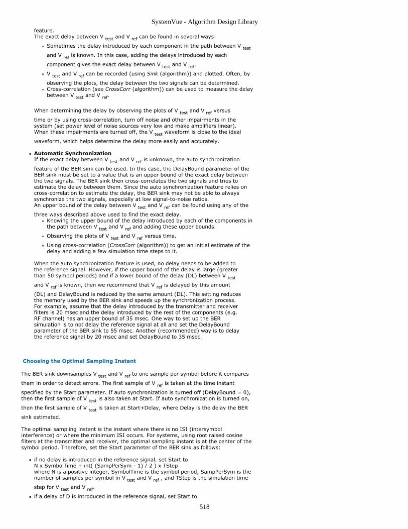
SystemVue - Algorithm Design Library
518
feature.The exact delay between V test and V ref can be found in several ways:
Sometimes the delay introduced by each component in the path between V test
and V ref is known. In this case, adding the delays introduced by each
component gives the exact delay between V test and V ref.
V test and V ref can be recorded (using Sink (algorithm)) and plotted. Often, by
observing the plots, the delay between the two signals can be determined.Cross-correlation (see CrossCorr (algorithm)) can be used to measure the delaybetween V test and V ref.
When determining the delay by observing the plots of V test and V ref versus
time or by using cross-correlation, turn off noise and other impairments in thesystem (set power level of noise sources very low and make amplifiers linear).When these impairments are turned off, the V test waveform is close to the ideal
waveform, which helps determine the delay more easily and accurately.
Automatic SynchronizationIf the exact delay between V test and V ref is unknown, the auto synchronization
feature of the BER sink can be used. In this case, the DelayBound parameter of theBER sink must be set to a value that is an upper bound of the exact delay betweenthe two signals. The BER sink then cross-correlates the two signals and tries toestimate the delay between them. Since the auto synchronization feature relies oncross-correlation to estimate the delay, the BER sink may not be able to alwayssynchronize the two signals, especially at low signal-to-noise ratios.An upper bound of the delay between V test and V ref can be found using any of the
three ways described above used to find the exact delay.Knowing the upper bound of the delay introduced by each of the components inthe path between V test and V ref and adding these upper bounds.
Observing the plots of V test and V ref versus time.
Using cross-correlation (CrossCorr (algorithm)) to get an initial estimate of thedelay and adding a few simulation time steps to it.
When the auto synchronization feature is used, no delay needs to be added tothe reference signal. However, if the upper bound of the delay is large (greaterthan 50 symbol periods) and if a lower bound of the delay (DL) between V test
and V ref is known, then we recommend that V ref is delayed by this amount
(DL) and DelayBound is reduced by the same amount (DL). This setting reducesthe memory used by the BER sink and speeds up the synchronization process.For example, assume that the delay introduced by the transmitter and receiverfilters is 20 msec and the delay introduced by the rest of the components (e.g.RF channel) has an upper bound of 35 msec. One way to set up the BERsimulation is to not delay the reference signal at all and set the DelayBoundparameter of the BER sink to 55 msec. Another (recommended) way is to delaythe reference signal by 20 msec and set DelayBound to 35 msec.
Choosing the Optimal Sampling Instant
The BER sink downsamples V test and V ref to one sample per symbol before it compares
them in order to detect errors. The first sample of V ref is taken at the time instant
specified by the Start parameter. If auto synchronization is turned off (DelayBound = 0),then the first sample of V test is also taken at Start. If auto synchronization is turned on,
then the first sample of V test is taken at Start+Delay, where Delay is the delay the BER
sink estimated.
The optimal sampling instant is the instant where there is no ISI (intersymbolinterference) or where the minimum ISI occurs. For systems, using root raised cosinefilters at the transmitter and receiver, the optimal sampling instant is at the center of thesymbol period. Therefore, set the Start parameter of the BER sink as follows:
if no delay is introduced in the reference signal, set Start toN x SymbolTime + int( (SampPerSym - 1) / 2 ) x TStepwhere N is a positive integer, SymbolTime is the symbol period, SampPerSym is thenumber of samples per symbol in V test and V ref , and TStep is the simulation time
step for V test and V ref.
if a delay of D is introduced in the reference signal, set Start to

SystemVue - Algorithm Design Library
519
N x SymbolTime + int( (SampPerSym - 1) / 2 ) x TStep + D
If your system has differential encoding/decoding, synchronization loops, carrier recoverysub-systems, or other sub-systems that need time to reach their steady state, set N to avalue that is large enough to enable the entire system to reach steady state.
Scaling of Test and Reference Signals
If the automatic threshold setting is used (BER sink ThresholdSetting parameter set toautomatically ) then the error detection thresholds are set to (2 x i - N ) / N, i = 1, 2, ...,N, where N is the number of thresholds (BER sink NumThresholds parameter).NumThresholds must be set to the number of signal levels minus 1 (3 for 4-PAM, 7 for 8-PAM, 3 for 16-QAM (3 levels per axis), 7 for 64-QAM (7 levels per axis)). The expectedsignal levels are located at the midpoints between the thresholds, that is at (2 x i - 2 - N)/ N, i = 1, 2, ... , N + 1. Both V test and V ref must be scaled appropriately so that when
these are sampled at the optimal sampling instant and assuming ideal conditions (no noiseor other distortions) these generate samples at the expected levels. Turning off the noiseand the rest of the impairments in the system and plotting the eye diagrams for Vtest andVref can help determine the signal levels at the optimal sampling instant and therefore,the appropriate scale factors.
References
J. Baprawski, "Generalized Modulation Mathematics Applied to RF System1.Simulation," Proceedings of the RF Expo West Conference, Santa Clara, CA, February5-7, 1991, pp. 127-147.T. T. Ha, Digital Satellite Communications, McGraw-Hill, 1990.2.N. Kanaglekar, et al. "Wave Analysis of Noise in Interconnected Multiport Networks,"3.IEEE Transactions on Microwave Theory and Techniques, Vol. MTT-35, No. 2,February 1987, pp. 112-115.D. Lu and J. Baprawski, "The Quasi-Analytical Method for Estimating Error4.Probabilities of M-ary Signaling Systems with Intersymbol Interference," Proceedingsof the 13th Symposium on Information Theory and its Applications , Tateshina,Japan, January 23-25, 1991, pp. 109-114.D. Lu and K. Yao, "Improved Importance Sampling Technique for Efficient Simulation5.of Digital Communication," IEEE Journal on Selected Areas in Communication, J-SAC,Vol. 6, No. 1, January 1988, pp. 67-75.R. W. Lucky, J. Salz and E. J. Weldon, Jr., Principles of Data Communications,6.McGraw-Hill, 1968.P. Z. Peebles, Jr., Digital Communication Systems, Prentice-Hall, 1987.7.G. Proakis, Digital Communication, McGraw-Hill, 1989.8.K. S. Shanmugan, Digital and Analog Communication Systems, John Wiley & Sons,9.1985.B. Sklar, Digital Communications, Prentice-Hall, 1988.10.

SystemVue - Algorithm Design Library
520
BER_FER PartCategories: Sinks (algorithm)
The models associated with this part are listed below. To view detailed information on amodel (description, parameters, equations, notes, etc.), please click the appropriate link.
Model Description
BER_FER(algorithm)
Bit and Frame Error RateMeasurement
BER_FER (Bit and Frame Error Rate Measurement)
Description: Bit and Frame Error Rate MeasurementDomain: TimedC++ Code Generation Support: NOAssociated Parts: BER FER Part (algorithm)
Model Parameters
Name Description Default Units Type RuntimeTunable
Range
StartStopOption Sink collection mode:Auto, Samples, Time
Auto Enumeration NO
SampleStart Sample number to startdata collection
0 Integer NO [0:∞)
SampleStop Sample number to stopdata collection
Num_Samples- 1
Integer NO [SampleStart:∞)
SampleDelayBound Upper bound of delaybetween test and refinputs in number ofsamples
0 Integer NO [0:∞)
TimeStart Time to start datacollection
Start_Time s Float NO [0:∞)
TimeStop Time to stop datacollection
Stop_Time s Float NO [TimeStart:∞)
TimeDelayBound Upper bound of delaybetween test and refinputs
0 s Float NO [0:∞)
BitsPerFrame Bits per frame 100 Integer NO [1:∞)
EstRelVariance BER estimation relativevariance
0.01 Float YES [0:1)
StatusUpdatePeriod Status update period innumber of bits
1000 Integer NO [1:∞)
Input Ports
Port Name Description Signal Type Optional
1 ref reference bit stream int NO
2 test test bit stream int NO
Notes/Equations
The BER_FER model can be used to measure the BER (bit error rate) and FER (frame1.error rate) of a system. In some systems, FER is referred to as PER (packet errorrate) or BLER (block error rate). The input signals to the reference (REF) and test(TEST) inputs must be bit streams. The bit streams must be synchronized, otherwisethe BER/FER estimates are wrong.The Start parameter defines when data processing starts. The end of data processing2.depends on the settings of the Stop and EstRelVariance parameters:
If EstRelVariance is 0.0, then data processing ends when Stop is reached.If EstRelVariance is greater than 0.0, then data processing ends whenEstRelvariance is met or when Stop is reached. In this case, Stop acts as anupper bound on how long the simulation runs just in case the simulation takestoo long for EstRelVariance to be met. In this mode of operation, messages areprinted in the simulation log showing the value of estimation relative variance asthe simulation progresses. The EstRelVariance parameter can be used to controlthe quality of the BER estimate obtained. The lower the value of EstRelVariancethe more accurate the estimate is.For more details, refer to PE Measurement Concepts (algorithm). Note that theequation for the estimation relative variance described in this section assumesthat the errors happen randomly (as in the case of an AWGN channel) and not inbursts (as in the case of a fading channel).

SystemVue - Algorithm Design Library
521
The BitsPerFrame parameter sets the number of bits in each frame. A frame is3.considered to be in error if at least one of the bits in the frame is detectedincorrectly. If the bit errors are independent identically distributed events then BERand FER are related through the equation FER = 1 − (1 − BER)BitsPerFrame.To estimate BER/FER over an exact number of frames set EstRelVariance to 0.0 andStop to Start + N × BitsPerFrame − 1, where Start is the value of the Startparameter, BitsPerFrame is the value of the BitsPerFrame parameter and N is thenumber of frames to be simulated.The StatusUpdatePeriod parameter can be used to control how often estimation4.relative variance status messages are reported to the simulation log.For the theoretical BER expressions for commonly used modulation formats see5.Theoretical BER Curves (algorithm).
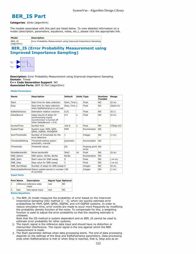
SystemVue - Algorithm Design Library
522
BER_IS PartCategories: Sinks (algorithm)
The models associated with this part are listed below. To view detailed information on amodel (description, parameters, equations, notes, etc.), please click the appropriate link.
Model Description
BER_IS(algorithm)
Error Probability Measurement using Improved Importance Sampling
BER_IS (Error Probability Measurement usingImproved Importance Sampling)
Description: Error Probability Measurement using Improved Importance SamplingDomain: TimedC++ Code Generation Support: NOAssociated Parts: BER IS Part (algorithm)
Model Parameters
Name Description Default Units Type RuntimeTunable
Range
Start Start time for data collection Start_Time s Float NO [0:∞)
Stop Stop time for data collectionwhen EstRelVariance is not met
Stop_Time s Float NO (Start:∞)
EstRelVariance Estimation relative variance 0.01 Float NO (0:1]
DelayBound Upper bound of delay forsynchronizing inputs(synchronizer is turned offwhen DelayBound = 0.0)
0.0 s Float NO [0:∞)
SymbolTime Symbol time 10e-6 s Float NO [TStep:∞)†
SystemType System type: PAM, QAM,QPSK, DQPSK, PI4DQPSK
PAM Enumeration NO
NumThresholds Number of thresholds for theerror detection
1 Integer NO [1:∞)
ThresholdSetting Threshold setting option:automatic, manual
automatic Enumeration NO
Thresholds Threshold values [0] Floating pointarray
NO
NoiseBandwidth Noise bandwidth 50e3 Hz Float NO (0:∞)
SNR_Option SNR option: Es/No, Eb/No Es/No Enumeration NO
SNR_Start Start value for SNR sweep 5 Float NO (-∞:∞)
SNR_Step Step value for SNR sweep 1 Float NO (-∞:∞)
SNR_NumSteps Number of steps for SNR sweep 5 Integer NO [0:∞)
StatusUpdatePeriod Status update period in numberof symbols
100 Integer NO [1:∞)
Input Ports
Port Name Description Signal Type Optional
1 reference reference datainput
real NO
2 test test signal input real NO
Notes/Equations
The BER_IS model measures the probability of error based on the Improved1.Importance Sampling (IIS) method [1 - 3], which can quickly estimate errorprobabilities for PAM, QAM, QPSK, DQPSK, and π/4-DQPSK systems. In order toreduce simulation time, error events are made to occur more frequently by modifyingthe probability density function of the noise. To compensate for this, a weightingfunction is used to adjust the error probability so that the resulting estimate isunbiased.Note that the IIS method is system dependent and so BER_IS cannot be used toestimate error probability for other systems.The input1 signal is the reference data input and should have no distortion or2.intersymbol interference. The input2 signal is the one against which the BERmeasurement is made.The Start parameter defines when data processing starts. The end of data processing3.depends on the settings of the Stop and EstRelVariance parameters. Data processingends when EstRelvariance is met or when Stop is reached, that is, Stop acts as an

SystemVue - Algorithm Design Library
523
upper bound on how long the simulation runs just in case the simulation takes toolong for EstRelVariance to be met.The EstRelVariance parameter is used to control the quality of the BER estimate4.obtained. The lower the value of EstRelVariance the more accurate the estimate isand the longer the simulation runs. For more details, refer to PE MeasurementConcepts (algorithm). Note that the equation for the estimation relative variancedescribed in this section assumes that the errors happen randomly (as in the case ofan AWGN channel) and not in bursts (as in the case of a fading channel).The Start parameter also defines the first sampling instant for the test and reference5.signals and therefore needs to be set so that the signals are sampled at the optimal,zero ISI (InterSymbol Interference) sampling instant. This is typically the center ofthe reference signal symbol period.
If the test and reference signals are already synchronized (DelayBound = 0)then they are sampled every SymbolTime sec starting at Start.If the test and reference signals are not synchronized (DelayBound parameter isgreater than 0) then the test signal is first synchronized to the reference signalby cross correlating them to estimate the delay between them. Then thereference signal is sampled every SymbolTime sec starting at Start and the testsignal is sampled every SymbolTime sec starting at Start + Delay, where Delayis the estimated delay between test and reference.
The DelayBound parameter specifies an upper bound for the delay between the test6.and reference signals. If DelayBound is set to 0, then the test and reference signalsare assumed to be synchronized and no synchronization is performed. If DelayBound> 0, then cross correlation is performed between the test and reference signals todetermine the delay between them. In this case, DelayBound is used as themaximum lag at which the cross correlation is computed. If the actual delay betweentest and reference is bigger than DelayBound, the simulation results will beunexpected.The SymbolTime parameter defines the symbol duration and is used to sample the7.input signals once in every symbol period.The SystemType parameter defines the modulation type used in the system. As8.mention earlier, the IIS method is system dependent.When SystemType is PAM or QAM then the number of detection thresholds needs to9.be specified in the NumThresholds parameter. NumThresholds is one less than thenumber of levels. For example, for a PAM-4 system, there are 4 levels and 3thresholds. For a 64-QAM system, there are 8 levels (on each axis) and 7 thresholds.The ThresholdSetting parameter defines how the detection thresholds are set.10.
If ThresholdSetting is set to automatic, then the thresholds are set at equaldistance between the ideal signal levels, which are assumed to be equallyspaced between -1 and 1. For example, for a PAM-4 system, the ideal levels are-1, -1/3, 1/3, 1 and so the thresholds are set to -2/3, 0, 2/3.If ThresholdSetting is set to manual, then the thresholds need to be specified inthe Thresholds array parameter. The values of the Thresholds array must bebetween -1 and 1 and they should be sorted in increasing order.In either case, the reference signal needs to be scaled so that whendownsampled (once every symbols period) it is in the range [-1, 1]. The testsignal also needs to be scaled so that when downsampled (once every symbolsperiod) it is in the range [-1, 1] if there is no distortion (ISI, distortion fromnon-linearities, etc). If distortion is present then the downsampled test signalwill be slightly outside the range [-1, 1] but this should be due only to distortionand not to gain (signal amplification/attenuation) factors between the point ofthe reference generation and the point of detection.
The BER_IS model adds white Gaussian noise to the test signal (there is no need for11.an external noise source). The NoiseBandwidth parameter is used in the calculationof the noise variance. To get the theoretical results in an AWGN (Additive WhiteGaussian Noise) environment, set NoiseBandwidth to one half of the symbol rate ( 1 /(2 × SymbolTime ) ). The noise variance also depends on the SNR value. Since theBER_IS model adds noise to the signal internally it can reuse the same input signalsand sweep the noise power to generate an entire BER waterfall curve. TheSNR_Start, SNR_Stop, and SNR_Step parameters are used to set this internal sweep.The SNR_Option parameter specifies whether the SNR values are E s / N o or E b / N o.
The StatusUpdatePeriod parameter controls how often status messages are printed to12.the simulation log. These messages show the value of the estimation relativevariance for the highest SNR as the simulation progresses. In addition, to thesemessages every time the estimation relative variance is met for a specific SNR value,a message is printed in the simulation log and that SNR value is removed from theinternal SNR sweep. This parameter does not affect the simulation results. It onlycontrols the frequency of the messages in the simulation log.Symbol Error Probability and Bit Error Probability13.The BER_IS model can measure the symbol error probability or symbol error rate P se
for a single channel. For a system with only one channel, such as PAM, the bit errorprobability or bit error rate P be can be calculated by P be = P se / L, where L is the
number of bits per symbol (for example, for a PAM-8 system L = 3). Note that theabove formula assumes that Gray coding was used to map the bits to symbols andthat symbol errors occur only between adjacent symbols, so that a symbol errortranslates to one bit error.

SystemVue - Algorithm Design Library
524
For systems with I and Q channels, such as QAM, QPSK, π/4-DQPSK, two BER_ISmodels must be used to measure the symbol error rate for each channel, P seI and P
seQ. Then P se for the whole system can be calculated by P se = P seI + P seQ − P seI
× P seQ.
To calculate the bit error rate P be for a system with two channels, first calculate the
bit error rate for each channel P beI and P beQ using the equations P beI = P seI / L
and P beQ = P seQ / L, where L is the number of bits per symbol in each channel (for
example, for QPSK L = 1, for 16-QAM L = 2, for 64-QAM L = 3). Again, theassumptions that Gray coding was used to map the bits to symbols and that symbolerrors occur only between adjacent symbols are made. After P beI and P beQ have
been calculated, the bit error rate for the whole system is given by P be = (P beI + P
beQ) / 2.
Simulation Time Improvement with IIS Simulation14.For a QAM system with a bit error rate of 10 -6, a Monte Carlo simulation requiresapproximately 10 8 bits for a reasonable accuracy (estimation relative variance of0.01). For the same system and accuracy an IIS simulation requires only 800 bits[1].Here are some steps to follow in order to set up a successful BER simulation using15.BER_IS:
Scale the test and reference signals appropriately as explained in note 9.Decide whether you will synchronize the test and reference signals manually oryou will use the synchronization feature of the BER_IS model.If you decide to synchronize the test and reference signals manually
determine the delay between them (this can be done by using theCrossCorr model or by plotting the two signals and visually estimating thedelay)delay (using the Delay model) the reference signal by the delay determinedconnect the delayed reference signal to the reference inputconnect the test signal to the test inputset the DelayBound parameter to 0
If you decide to use the synchronization feature of the BER_IS modeldetermine an upper bound of the delay between the test and referencesignals (this can be done by using the CrossCorr model or by plotting thetwo signals and visually estimating the delay)connect the reference signal to the reference inputconnect the test signal to the test inputset the DelayBound parameter to the upper bound of the delay youdetermined
Set the Start parameter to the center of the symbol period of the referencesignal. If you have manually synchronized the test and reference signals byadding delay in the reference signal make sure you account for this delay whensetting Start.Set the Stop parameter to an upper bound of how much time you want tosimulate.Set the EstRelVariance parameter to the desired value for the accuracy youwant.Set SymbolTime, SystemType, and NumThresholds based on the system youwant to simulate.Decide whether to use automatic or manual threshold setting and set theThresholdSetting and Thresholds parameters accordingly.Set the NoiseBandwidth parameter to the noise bandwidth of your system. Fortheoretical results in an AWGN environment NoiseBandwidth must be set to onehalf of the symbol rate ( 1 / (2 × SymbolTime ) ).Set SNR_Option, SNR_Start, SNR_Step, and SNR_NumSteps to the appropriatevalues that will generate the BER waterfall curve you want.Set StatusUpdatePeriod to the desired value.
For the theoretical BER expressions for commonly used modulation formats see16.Theoretical BER Curves (algorithm).For general information regarding sinks, refer to About Sinks (algorithm).17.
References
D. Lu and K. Yao, "Improved Importance Sampling Technique for Efficient Simulation1.of Digital Communication Systems," IEEE J. Select. Areas Commun. vol. 6, pp. 67-75, Jan. 1988.D. Lu and K. Yao, "Estimation Variance Bounds of Importance Sampling Simulations2.in Digital Communication Systems," IEEE Trans. Commun. vol 39, pp. 1413-1417,Oct. 1991.J. Chen, D. Lu, J. Sadowski, and K. Yao "On Importance Sampling in Digital3.Communications - Part I: Fundamentals," IEEE J. Select. Areas in Commun. vol 11.No. 3, pp. 289-299, April, 1993.

SystemVue - Algorithm Design Library
525
CCDF PartCategories: Sinks (algorithm)
The models associated with this part are listed below. To view detailed information on amodel (description, parameters, equations, notes, etc.), please click the appropriate link.
Model Description
CCDF_Env(algorithm)
Complementary Cumulative Distribution Function (CCDF)
CCDF_Cx (algorithm) Complementary Cumulative Distribution Function (CCDF)
CCDF_Cx
Description: Complementary Cumulative Distribution Function (CCDF)Domain: TimedC++ Code Generation Support: NOAssociated Parts: CCDF Part (algorithm)
Model Parameters
Name Description Default Units Type RuntimeTunable
Range
Start Start time for data collection Start_Time s Float NO [0:∞)
Stop Stop time for data collection Stop_Time s Float NO [Start:∞)
NumBins Number of points in the CCDFcurve
100 Integer NO [3:65535]
OutputPeakMean Output signal peak and meanvalues: NO, YES
NO Enumeration NO
Input Ports
Port Name Description Signal Type Optional
1 input input signal complex NO
Notes/Equations
The CCDF_Cx model computes the complementary cumulative distribution function1.(CCDF) of a complex signal. As its name suggests, CCDF is the complement of thecumulative distribution function (CDF). The relationship between CCDF and CDF isCCDF = 1 - CDF.The calculation of the CCDF is described below:
Calculate the RMS value for all measured samples; this becomes the 0 dB pointon the x-axis.Normalize all samples to the RMS value in units of dB.Split the x-axis in equal width NumBin bins starting from minimum measuredpower to maximum measured power.Determine which x-axis bin each sample belongs to.Calculate the total number of samples that are greater than or equal to each x-axis bin and output it as a percent of the number of samples measured.
In addition to the CCDF measurement, this model can provide PeakPower (the peak2.power for the input signal) and MeanPower (the mean or average power of the inputsignal). To compute and output MeanPower and PeakPower, set the parameterOutputPeakMean to YES.The CCDF measurement is a very common measurement performed on 2G, 3G and3.4G wireless signals. The CCDF curve shows the probability that the instantaneoussignal power will be higher than the average signal power by a certain amount of dB.The independent axis of the CCDF curve shows power levels in dB with respect to theaverage signal power level (0 dB corresponds to the average signal power level). Thedependent axis of the CCDF curve shows the probability that the instantaneous signalpower exceeds the corresponding power level on the independent axis. The followingfigure shows the CCDF curve for a WiMax 802.16e Downlink signal. In the figure, youcan see that the instantaneous signal power exceeds the average signal power (0 dB)for 35% of the time. You can also see that the instantaneous signal power exceedsthe average signal power by 5 dB for only 7% of the time.
CCDF measurement for a WiMax 802.16e Downlink Signal

SystemVue - Algorithm Design Library
526
The amount of data collected and on which the CCDF measurement is performed is4.controlled by the Start and Stop parameters. Data collection always begins at thetime instant specified by Start and ends at the time instant specified by Stop.In most wireless communication systems with framed or burst data, the CCDF5.measurement must be performed on the active part of the signal (idle parts betweenframes/burst should be excluded).For general information regarding sinks, refer to About Sinks (algorithm).6.
See:CCDF_Env (algorithm)
CCDF_Env
Description: Complementary Cumulative Distribution Function (CCDF)Domain: TimedC++ Code Generation Support: NOAssociated Parts: CCDF Part (algorithm)
Model Parameters
Name Description Default Units Type RuntimeTunable
Range
Start Start time for data collection Start_Time s Float NO [0:∞)
Stop Stop time for data collection Stop_Time s Float NO [Start:∞)
NumBins Number of points in the CCDFcurve
100 Integer NO [3:65535]
OutputPeakMean Output signal peak and meanvalues: NO, YES
NO Enumeration NO
Input Ports
Port Name Description Signal Type Optional
1 input input signal envelope NO
Notes/Equations
The CCDF_Env model computes the complementary cumulative distribution function1.(CCDF) of an envelope signal. For more details on the CCDF measurement seeCCDF_Cx (algorithm).For general information regarding sinks, refer to About Sinks (algorithm).2.
See:CCDF_Cx (algorithm)
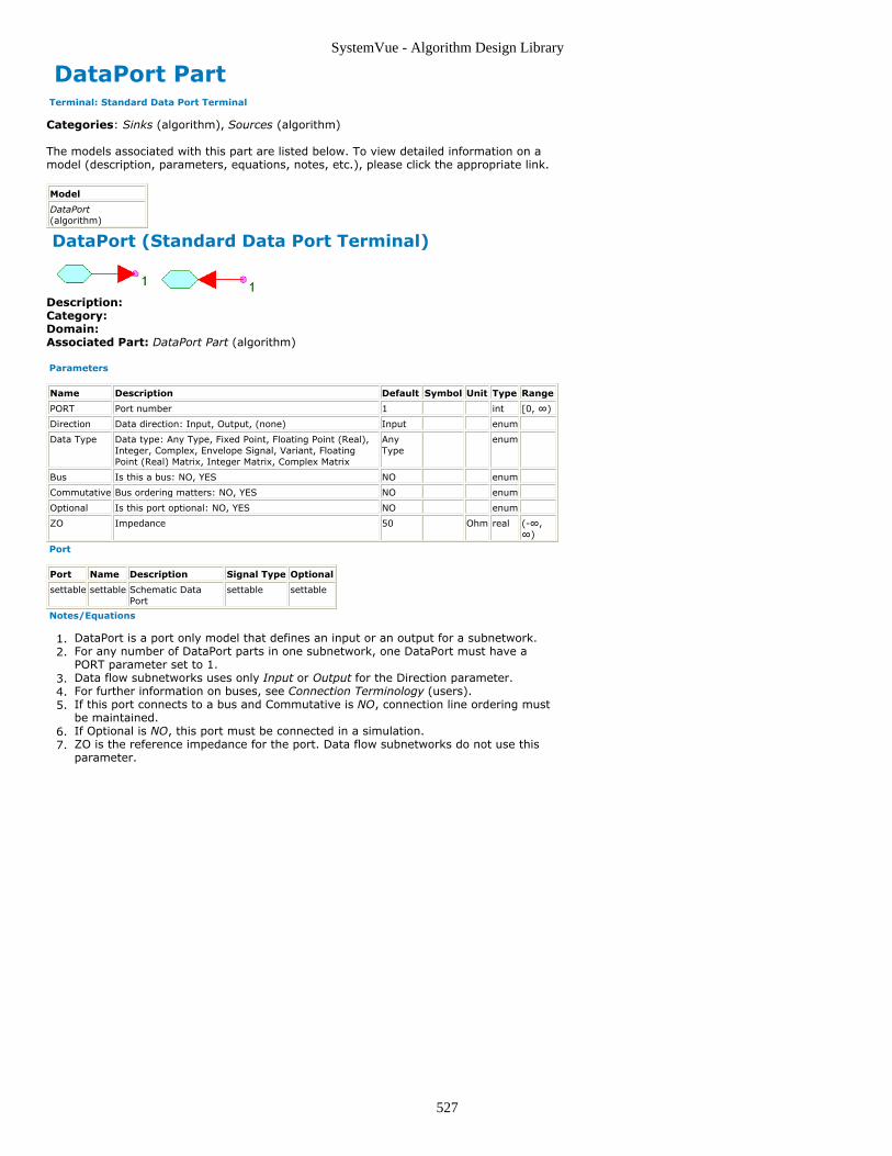
SystemVue - Algorithm Design Library
527
DataPort Part Terminal: Standard Data Port Terminal
Categories: Sinks (algorithm), Sources (algorithm)
The models associated with this part are listed below. To view detailed information on amodel (description, parameters, equations, notes, etc.), please click the appropriate link.
Model
DataPort(algorithm)
DataPort (Standard Data Port Terminal)
Description:Category:Domain:Associated Part: DataPort Part (algorithm)
Parameters
Name Description Default Symbol Unit Type Range
PORT Port number 1 int [0, ∞)
Direction Data direction: Input, Output, (none) Input enum
Data Type Data type: Any Type, Fixed Point, Floating Point (Real),Integer, Complex, Envelope Signal, Variant, FloatingPoint (Real) Matrix, Integer Matrix, Complex Matrix
AnyType
enum
Bus Is this a bus: NO, YES NO enum
Commutative Bus ordering matters: NO, YES NO enum
Optional Is this port optional: NO, YES NO enum
ZO Impedance 50 Ohm real (-∞,∞)
Port
Port Name Description Signal Type Optional
settable settable Schematic DataPort
settable settable
Notes/Equations
DataPort is a port only model that defines an input or an output for a subnetwork.1.For any number of DataPort parts in one subnetwork, one DataPort must have a2.PORT parameter set to 1.Data flow subnetworks uses only Input or Output for the Direction parameter.3.For further information on buses, see Connection Terminology (users).4.If this port connects to a bus and Commutative is NO, connection line ordering must5.be maintained.If Optional is NO, this port must be connected in a simulation.6.ZO is the reference impedance for the port. Data flow subnetworks do not use this7.parameter.

SystemVue - Algorithm Design Library
528
EVM PartCategories: Sinks (algorithm)
The models associated with this part are listed below. To view detailed information on amodel (description, parameters, equations, notes, etc.), please click the appropriate link.
Model Description
EVM_Env(algorithm)
Error Vector MagnitudeMeasurement
EVM_Cx (algorithm) Error Vector MagnitudeMeasurement

SystemVue - Algorithm Design Library
529
EVM_Cx
Description: Error Vector Magnitude MeasurementDomain: TimedC++ Code Generation Support: NOAssociated Parts: EVM Part (algorithm)
Model Parameters
Name Description Default Units Type RuntimeTunable
Range
Start Start time for datacollection
Start_Time s Float NO [0:∞)
SymTime Symbol durationtime
10e-6 s Float NO [TStep:1000*TStep]†
SymBurstLen Burst length innumber ofsymbols
100 Integer NO [1:∞)
MeasType Measurementtype: EVM RMS,EVM Peak, C0,Frequency error,Droop, Errorsequence,Magnitude errorsequence, Phaseerror sequence,Sampled data
EVM RMS Enumeration NO
ModType Modulation type:BPSK, QPSK,HPSK, PI/4DQPSK, PSK8,PSK16, QAM4,QAM16, QAM32,QAM64, QAM128,QAM256, PAM4,PAM8, Userdefined
QPSK Enumeration NO
Constellation Complexconstellationvalues
[1+j, 1-j, -1-j, -1+j]
Complexarray
NO
OptimizeSamplingInstant Automatically findoptimal samplinginstant: NO, YES
YES Enumeration NO
Input Ports
Port Name Description Signal Type Optional
1 input input signal complex NO
Notes/Equations
The EVM_Cx model is used to perform an EVM (Error Vector Magnitude)1.measurement for a complex signal. EVM measurements are used to evaluate themodulation accuracy of modulators. It is used, for example, in the IS-54 TDMA digitalcellular to set the minimum specifications for modulation accuracy of π/4-DQPSKmodulators.The defining equations for the EVM measurement follow the definition in the EIA/TIAIS-54-B TDMA Cellular System Dual-Mode Mobile Station-Base Station CompatibilityStandard, section 2.1.3.3.1.3.3 (Error Vector Magnitude Requirement). Let Z(k)denote the actual complex vectors (I and Q) produced by observing the realtransmitter through an ideal receiver filter at instants k, one symbol period apart.S(k) is defined as the ideal reference symbol (normalized such that its maximumenergy symbol falls on the unit circle). Then, Z(k) is modeled as:
where
W = e Dr+jDa , accounts for both a frequency offset (Da radians/symbolphase rotation) and an amplitude change rate (of Dr nepers/symbol)
C0 is a complex constant origin offset (in Volts)
C1 is a unitless complex constant representing the arbitrary phase and

SystemVue - Algorithm Design Library
530
output power of the transmitter, and
E(k) is the residual vector error on sample S(k) (in Volts)
The sum square error vector is
where N is equal to SymBurstLen and C 0 , C 1 , W are chosen such as to minimize
the above expression.EVM (rms) is defined to be the rms value of | E(k) | normalized by the rms value of |S(k) |. Therefore,
The symbol EVM at symbol k is defined as
which is the vector error magnitude at symbol k normalized by the rms value of |S(k) |.The MeasType parameter determines the output of the component.2.
If MeasType = EVM RMS, the output is the EVM(rms) value as defined in theequations of note 1. This value is not in percent.To get EVM RMS in percent,multiply by 100.If MeasType = EVM Peak, the output is max{ EVM(k) }, where the maximum isevaluated over k = 0, 1, ... , N-1. This value is not in percent.To get EVM Peakin percent, multiply by 100.If MeasType = C0, the output is
dBIf MeasType = Frequency error, the output is
HzIf MeasType = Droop, the output is
dBIf MeasType = Error sequence, the output is the sequence
If MeasType = Magnitude Error sequence, the output is the magnitude errorsequence (in Volts). For the definition of magnitude error, see the followingfigure.If MeasType = Phase Error sequence, the output is the phase error sequence (indegrees). For the definition of phase error, see the following figure.If MeasType = Sampled data, the output is the downsampled (1 sample persymbol period) input signal.
Magnitude and Phase Error
The ModType parameter is used to select one of the pre-defined or a user-defined3.signal constellation. All signal constellations (including user- defined) are normalizedso that the maximum magnitude constellation point lies on the unit circle. Forexample, for a QPSK constellation, all four IQ points lie on the unit circle.For a PAM-type signal (includes BPSK, 4-PAM, 8-PAM) the Q-channel of the signal isset to 0.0.The following figure shows a few examples of the IQ constellation sets used in theEVM measurement.The HPSK option is for an HPSK signal that has equal gains applied to the I and Qchannels resulting in a 4-point constellation. In effect, this is the same as a QPSKconstellation. If the gains applied to the I and Q channels are different, the resultingconstellation has 8 points and using the HPSK option gives the wrong results; in this

SystemVue - Algorithm Design Library
531
case, the User defined option should be used, which enables you to specify anarbitrary constellation in the Constellation parameter.The Start and OptimizeSamplingInstant parameters define how the input signal is4.downsampled. Note that the EVM algorithm operates on the downsampled inputsignal.If OptimizeSamplingInstant is set to NO, the input signal is downsampled at onesample per symbol period starting at Start. If Start is not an exact multiple of thesimulation time step, interpolation is used to find the input signal values in betweenthe available samples.If OptimizeSamplingInstant is set to YES, the input signal is downsampled at onesample per symbol period starting at StartDownSampling, where StartDownSamplingis swept from Start to ( Start + SymTime ) with a step of (simulation time step) / 10.This way the optimal sampling instant can be found. The optimal value forStartDownSampling is displayed on the status window and can be used in subsequentsimulations as the value of Start with OptimizeSamplingInstant set to NO. Thissetting results in faster simulations and gives the correct results as long as noparameter that can affect the optimal sampling instant (for example the delay of afilter) is changed. If such a parameter changes, then OptimizeSamplingInstant shouldbe set to YES.Another way to find when the optimal sampling instant is, without setting theOptimizeSamplingInstant parameter to YES, is to observe the eye diagram and findwhere its maximum opening occurs.
Examples of IQ-Constellations as Used in EVM Measurement
For general information regarding sinks, refer to About Sinks (algorithm).5.
See:EVM_Env (algorithm)

SystemVue - Algorithm Design Library
532
EVM_Env
Description: Error Vector Magnitude MeasurementDomain: TimedC++ Code Generation Support: NOAssociated Parts: EVM Part (algorithm)
Model Parameters
Name Description Default Units Type RuntimeTunable
Range
Start Start time for datacollection
Start_Time s Float NO [0:∞)
SymTime Symbol durationtime
10e-6 s Float NO [TStep:1000*TStep]†
SymBurstLen Burst length innumber ofsymbols
100 Integer NO [1:∞)
MeasType Measurementtype: EVM RMS,EVM Peak, C0,Frequency error,Droop, Errorsequence,Magnitude errorsequence, Phaseerror sequence,Sampled data
EVM RMS Enumeration NO
ModType Modulation type:BPSK, QPSK,HPSK, PI/4DQPSK, PSK8,PSK16, QAM4,QAM16, QAM32,QAM64, QAM128,QAM256, PAM4,PAM8, Userdefined
QPSK Enumeration NO
Constellation Complexconstellationvalues
[1+j, 1-j, -1-j, -1+j]
Complexarray
NO
OptimizeSamplingInstant Automatically findoptimal samplinginstant: NO, YES
YES Enumeration NO
Input Ports
Port Name Description Signal Type Optional
1 input input signal envelope NO
Notes/Equations
The EVM_Env model is used to perform an EVM (Error Vector Magnitude)1.measurement for an envelope signal. For more details on the EVM measurement seeEVM_Cx (algorithm).For general information regarding sinks, refer to About Sinks (algorithm).2.
See:EVM_Cx (algorithm)

SystemVue - Algorithm Design Library
533
FlexDCA_Sink PartCategories: Sinks (algorithm)
The models associated with this part are listed below. To view detailed information on amodel (description, parameters, equations, notes, etc.), please click the appropriate link.
Model Description
FlexDCA_Sink(algorithm)
Stream simulation samples to the Agilent FlexDCAApplication
FlexDCA_Sink
Description: Stream simulation samples to the Agilent FlexDCA ApplicationDomain: TimedC++ Code Generation Support: NOAssociated Parts: FlexDCA Sink Part (algorithm)
Model Parameters
Name Description Default Units Type RuntimeTunable
NumberOfInputs Number of inputs. 1 Integer NO
ContinuousMode Run simulation continuously.: NO,YES
YES Enumeration NO
NumBitsToSkip Number of bits to skip beforewriting to text file.
0 Integer NO
NumPatternToSimulate Number of patterns to simulate. 1 Integer NO
BitRate Original bit rate. Sample_Rate Hz Float NO
PatternLength Number of bits per period forperiodic bit pattern.
127 Integer NO
AdvancedParameters Display advanced parameters.: NO,YES
NO Enumeration NO
SetupFile Name of setup file to recall Filename NO
Simulation start always sets FlexDCA to Eye mode. The reason is that the amount of data bufferedfor jitter analysis is many magnitudes higher than the amount needed for Eye or Scope mode. By startingFlexDCA in Eye mode, old data can be quickly flushed out of the buffer. For the same reason, if transientis observed in Jitter mode to make eye closed, switch to Eye mode until eye diagram is clearbefore switching back to Jitter mode.
No more than one FlexDCA_Sink can be placed on the same schematic.
Before you start SystemVue, make sure FlexDCA software is not already running.
FlexDCA requires patterned (periodic) bits for jitter analysis. For example, use PRBS (algorithm) modelin Bits Part (algorithm) for the bit source.
FlexDCA_Sink UI Properties
If desired, click the Advanced Options ... button on the bottom left corner of FlexDCA_Sink UI to viewthe parameter list. The mapping between the parameters in the parameter list and the setup controlsshown in the Graphic User Interface described here should be straightforward.
Most of the setup controls in the User Interface is self explanatory. In the following weonly cover a few key setup controls.
Number of Inputs FlexDCA can support up to 8 channels of inputs. Specify how1.many channels are desired and the input pins on the placed part will adjustaccordingly.Number of Bits to Skip Specify how many bits to skip before streaming the data to2.FlexDCA. Typically it is used to avoid sending transient data into the FlexDCA.Pattern Length FlexDCA requires patterned (periodic) bits for jitter analysis, so3.provide pattern length here. For example, if you use PRBS (algorithm) model inBits Part (algorithm) as the bit source and the LFSR_Length is 12, then the patternlength is 2^12 - 1 = 4095.Run Simulation Continuously By default, simulation will run continuously and4.streaming bits into FlexDCA. If unchecked, please specify how many patterns tosimulate.

SystemVue - Algorithm Design Library
534
FlexDCA Control Basics
Color Grade Display To have the Eye diagram displayed in color grade, mouse rightclick on the eye diagram area, then select "Color Grade" as shown here:

SystemVue - Algorithm Design Library
535
Mode Selection Either use menu "Setup -> Mode" or the big ellipse-shaped buttonon the top-right corner of the display. The simulation will always set FlexDCA to itsEye mode.
A separate license has to be purchased in order to use the Jitter mode.
Channel Selection Notice a row of rectangle areas on the bottom side of thedisplay. Click on any one of the 4 rectangles on the right side will bring up a channelactivation dialog that looks like the following. Toggle the round shaped button to turnON/OFF the display for the channel.
In Jitter mode (which needs a separate license), only one channel can be active.
Auto-Scale Use menu "Control -> Auto Scale" to auto-scale the displays asneeded (e.g. if the Eye diagram is not centered).Pattern Parameters Critical pattern parameters such as Pattern Length and DataRate are set up automatically at the start of simulation. However, you can modifythem during simulation by clicking on the Trigger rectangle and go to the PatternLock Setup tab of the dialog opened as shown here.
At simulation start, these parameters will be reset by the simulation. Also, all the "Auto Detect"functions (and their corresponding check boxes) are disabled by the simulation.
Notes/Links
An example of using FlexDCA_Sink can be found in IBIS AMI Modeling.wsv under1.Model Building Examples (examples)To learn about FlexDCA, go to http://www.agilent.com/find/flexdca2.To download FlexDCA software, go to3.

SystemVue - Algorithm Design Library
536
http://www.agilent.com/find/flexdca_download
Printer (Data File Writer)
Description: Data File WriterCategory: SinksDomain: TimedAssociated Part:
Parameters
Name Description Default Symbol Unit Type Range
StartStopOption Sink collection mode: Auto,Samples, Time
Auto enum
SampleStart Sample number to start datacollection
0 int [0,∞)
SampleStop Sample number to stop datacollection
Num_Samples -1
int [SampleStart,∞)
TimeStart Time to start data collection Start_Time sec real [0,∞)
TimeStop Time to stop data collection Stop_Time sec real [TimeStart,∞)
File Output filename 'print.txt' filename
Input Ports
Port Name Description Signal Type Optional
1 input input signal multiple anytype NO
Notes/Equations
Printer prints out one sample from each input port per line.1.The output file is a text file that contains data in ADS Ptolemy format specific to the2.input data type: real array (for floating-point (real), fixed, and integer scalar inputdata), complex array, string array, real matrix, integer matrix, fixed-point matrix, orcomplex matrix. For format information, refer to Understanding File Formats in theADS Ptolemy Simulation manual.For general information regarding sinks, refer to About Sinks (algorithm).3.

SystemVue - Algorithm Design Library
537
RMSE PartCategories: Sinks (algorithm)
The models associated with this part are listed below. To view detailed information on amodel (description, parameters, equations, notes, etc.), please click the appropriate link.
Model Description
RMSE(algorithm)
Root Mean Square Error Measurement
RMSE (Root Mean Square Error Measurement)
Description: Root Mean Square Error MeasurementDomain: UntimedC++ Code Generation Support: NOAssociated Parts: RMSE Part (algorithm)
Model Parameters
Name Description Default Units Type RuntimeTunable
Range
StartFrame Start frame 0 Integer NO [0:∞)
FramesToAverage Number of frames to measure 1 Integer NO [1:∞)
FrameLength Frame length in number ofsamples
Num_Samples Integer NO [1:∞)
DisplayOption Display option: RMS, dB RMS Enumeration NO
Input Ports
Port Name Description Signal Type Optional
1 InRef Input referencesignal
complex NO
2 InTest Input test signal complex NO
Notes/Equations
The RMSE model is used to calculate the root mean squared error between the two1.input signals.Input data is collected starting at sample StartFrame × FrameLength and ending at2.sample (FramesToAverage + StartFrame) × FrameLength − 1.The root mean square error is calculated according to the equation3.
where,Nf is the number of frames to average
Lf is the frame length
I1(i, j), Q1 (i, j) and I2 (i, j), Q2 (i, j) are the in-phase and quadrature parts,
respectively, of the input signals.If DisplayOption is set to RMS, then the value as calculated by the above equations is4.saved in the dataset. If DisplayOption is set to dB, then 20×log10( RMSE ) is savedin the dataset.

SystemVue - Algorithm Design Library
538
Sink PartCategories: Sinks (algorithm)
The models associated with this part are listed below. To view detailed information on amodel (description, parameters, equations, notes, etc.), please click the appropriate link.
Model Description
Sink(algorithm)
Data Sink

SystemVue - Algorithm Design Library
539
Sink (Data Sink)
Description: Data SinkDomain: TimedC++ Code Generation Support: NOAssociated Parts: Sink Part (algorithm)
Model Parameters
Name Description Default Units Type RuntimeTunable
Range
StartStopOption Sink collection mode:Auto, Samples, Time
Auto Enumeration NO
SampleStart Sample number tostart data collection
0 Integer NO [0:∞)
SampleStop Sample number tostop data collection
Num_Samples -1
Integer NO [SampleStart:∞)
TimeStart Time to start datacollection
Start_Time s Float NO [0:∞)
TimeStop Time to stop datacollection
Stop_Time s Float NO [TimeStart:∞)
SinkTarget Location wheresimulation data iswritten: DataSet, File,Both
DataSet Enumeration NO
ContinuousMode Run simulation incontinuous mode:NO, YES
NO Enumeration NO
WindowSize Number of samples tocollect and display indynamically updatedgraph
500 Integer NO [1:∞)
DisableDataCollect Disable the collectionof data: NO, YES
NO Enumeration NO
Graph Graph to display thedata in (if empty nograph is created)
Text NO
Table Table to display thedata in (if empty notable is created)
Text NO
ToSingleFile Write data from allinputs to the samefile: NO, YES
YES Enumeration NO
DataFileName Data file name SinkData Filename NO
DataFileType Data file format:ASCII, Binary,SignalStudio, N5106A
ASCII Enumeration NO
SkipFrequency Do not writecharacterizationfrequency (forcomplex envelopedata) to file: NO, YES
NO Enumeration NO
NormalizeWaveform Normalize inputsignal magnitude to[-1,1] range beforewriting to file: NO,YES
YES Enumeration NO
ClippingLevel Clipping voltage level 1.0 V Float NO (0:∞)
Persistence Keep sink data indataset whenworkspace is saved:NO, YES
Data_Persistence Enumeration NO
Input Ports
Port Name Description Signal Type Optional
1 input Input Signal multiple anytype NO
Important Note: When writing data to files, neither ASCII file nor Binary file is for use with otherAgilent products (such as VSA 89601A software). ASCII file is solely for logging simulation data whenneeded. Binary file is to temporarily store large amount of simulation data to be post processed byMathLang script (users). (See SignalDownloader_E4438C (algorithm) part as an example of how touse MathLang script (users) to post process Binary file).
Setup UIA custom UI is provided for this model that allows easy set up.
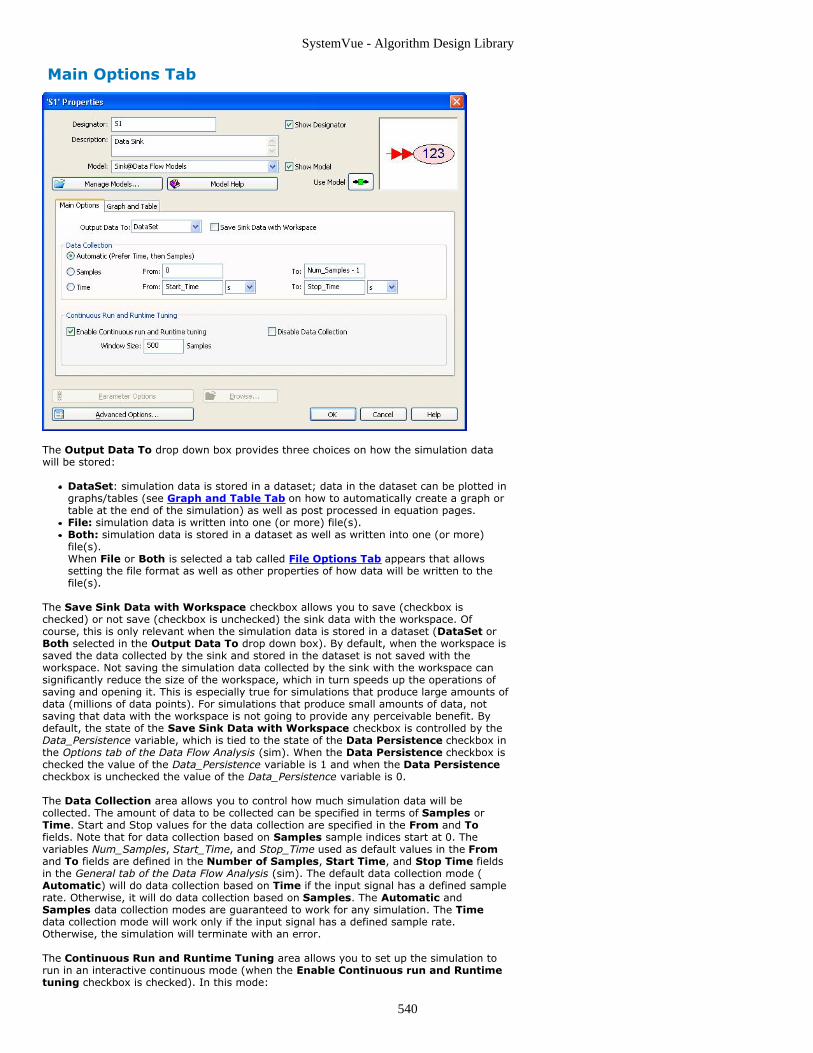
SystemVue - Algorithm Design Library
540
Main Options Tab
The Output Data To drop down box provides three choices on how the simulation datawill be stored:
DataSet: simulation data is stored in a dataset; data in the dataset can be plotted ingraphs/tables (see Graph and Table Tab on how to automatically create a graph ortable at the end of the simulation) as well as post processed in equation pages.File: simulation data is written into one (or more) file(s).Both: simulation data is stored in a dataset as well as written into one (or more)file(s).When File or Both is selected a tab called File Options Tab appears that allowssetting the file format as well as other properties of how data will be written to thefile(s).
The Save Sink Data with Workspace checkbox allows you to save (checkbox ischecked) or not save (checkbox is unchecked) the sink data with the workspace. Ofcourse, this is only relevant when the simulation data is stored in a dataset (DataSet orBoth selected in the Output Data To drop down box). By default, when the workspace issaved the data collected by the sink and stored in the dataset is not saved with theworkspace. Not saving the simulation data collected by the sink with the workspace cansignificantly reduce the size of the workspace, which in turn speeds up the operations ofsaving and opening it. This is especially true for simulations that produce large amounts ofdata (millions of data points). For simulations that produce small amounts of data, notsaving that data with the workspace is not going to provide any perceivable benefit. Bydefault, the state of the Save Sink Data with Workspace checkbox is controlled by theData_Persistence variable, which is tied to the state of the Data Persistence checkbox inthe Options tab of the Data Flow Analysis (sim). When the Data Persistence checkbox ischecked the value of the Data_Persistence variable is 1 and when the Data Persistencecheckbox is unchecked the value of the Data_Persistence variable is 0.
The Data Collection area allows you to control how much simulation data will becollected. The amount of data to be collected can be specified in terms of Samples orTime. Start and Stop values for the data collection are specified in the From and Tofields. Note that for data collection based on Samples sample indices start at 0. Thevariables Num_Samples, Start_Time, and Stop_Time used as default values in the Fromand To fields are defined in the Number of Samples, Start Time, and Stop Time fieldsin the General tab of the Data Flow Analysis (sim). The default data collection mode (Automatic) will do data collection based on Time if the input signal has a defined samplerate. Otherwise, it will do data collection based on Samples. The Automatic andSamples data collection modes are guaranteed to work for any simulation. The Timedata collection mode will work only if the input signal has a defined sample rate.Otherwise, the simulation will terminate with an error.
The Continuous Run and Runtime Tuning area allows you to set up the simulation torun in an interactive continuous mode (when the Enable Continuous run and Runtimetuning checkbox is checked). In this mode:

SystemVue - Algorithm Design Library
541
the simulation will keep running even after all the sinks have collected the data thathas been requestedfor each sink that has the Enable Continuous run and Runtime tuning checkboxchecked a dynamic plot is created where the input signal is plotted; since thedynamic plot can only plot a fixed number of samples (Window Size field) thewaveform will appear to be moving (just as in the case of an oscilloscope or vectorsignal analyzer) unless it is periodic and the Window Size is set to a value thatrepresents the exact number of samples in an integer number of periodsall parameters/variables that are tunable can be tuned while the simulation is runningthe data collection (in the dataset or file) can be optionally disabled (Disable DataCollection checkbox)
An example of a dynamic plot is shown below.
A right mouse click on the dynamic plot brings up a menu where you can
enable a marker; its coordinates X and Y are shown at the top right corner of the plotenable an offset (marker); the differences between its coordinates and thecoordinates of the marker are also shown at the top right corner of the plot (dX anddY)move the offset (marker) to the same point as the markerconfigure the axes; allows you to choose a number of different formats to bedisplayed: Log Mag (dB), Linear Mag, Real (I), Imag (Q), Wrap Phase, Unwrap Phase,I-Q, Constellation, Trelis-Eye, Group Delay, Log Mag (lin)set the Y-axis limits; allows you to select between auto-scaling the Y-axis or fixing itstop and bottom limits
File Options Tab

SystemVue - Algorithm Design Library
542
The Filename field sets the name of the file where the simulation data will be written. If arelative path is specified, then the path is relative to the directory where the workspace islocated. For a new workspace that has not been saved yet, the path is relative to theworkspace that was the starting point. For example, if you create a new workspacestarting with the Blank template then the paths are relative to the Templates directory ofyour SystemVue installation.
The Produce Separate Files for each Sink Input (add Suffix) checkbox allows (whenchecked) the creation of a separate file for each input signal. The first input signal usesthe filename that was entered in the Filename field. The other inputs use filenames withthe suffixes _1, _2, ... For example, if the filename entered is LTE.wfm, the second inputwill use filename LTE_1.wfm and so on. If this checkbox is not checked then all the inputsignals are saved in the same file.
The File Format drop down box is used to select the format of the file to be written. Thesupported formats are:
ASCII: This creates an ASCII text file with the values of the input signals. Each inputis written in its own column (if the Produce Separate Files for each Sink Input(add Suffix) checkbox is not checked). In addition, if the input signal has a definedsample rate, then the first column has the time stamps of the signal samples.Binary: In this format, every sample of the input signal is written to the file using 8bytes "double" format. If the input signal is complex, the real and imaginary partsare written in the order of: #1 Real, #1 Imaginary, #2 Real, #2 Imaginary, #3 Real,#3 Imaginary, ... When there are multiple input signals written into a single file (Produce Separate Files for each Sink Input (add Suffix) checkbox is notchecked), the order of the data is also impacted by the value of the Write to Fileevery ___ Samples field. Let's assume the sink has been set up to Write to Fileevery 10 Samples, and there are 3 complex input signals (s1, s2, s3). The order ofthe data in the file will be (the lines shown below separating the data points are onlyfor readability; binary files do not have a concept of lines):s1 #1 Real, s1 #1 Imaginary, s1 #2 Real, s1 #2 Imaginary, ..., s1 #10 Real, s1 #10Imaginary,s2 #1 Real, s2 #1 Imaginary, s2 #2 Real, s2 #2 Imaginary, ..., s2 #10 Real, s2 #10Imaginary,s3 #1 Real, s3 #1 Imaginary, s3 #2 Real, s3 #2 Imaginary, ..., s3 #10 Real, s3 #10Imaginary,s1 #11 Real, s1 #11 Imaginary, s1 #12 Real, s1 #12 Imaginary, ..., s1 #20 Real, s1#20 Imaginary,s2 #11 Real, s2 #11 Imaginary, s2 #12 Real, s2 #12 Imaginary, ..., s2 #20 Real, s2#20 Imaginary,s3 #11 Real, s3 #11 Imaginary, s3 #12 Real, s3 #12 Imaginary, ..., s3 #20 Real, s3#20 Imaginary,s1 #21 Real, s1 #21 Imaginary, s1 #22 Real, s1 #22 Imaginary, ..., s1 #30 Real, s1#30 Imaginary,s2 #21 Real, s2 #21 Imaginary, s2 #22 Real, s2 #22 Imaginary, ..., s2 #30 Real, s2#30 Imaginary,s3 #21 Real, s3 #21 Imaginary, s3 #22 Real, s3 #22 Imaginary, ..., s3 #30 Real, s3#30 Imaginary,

SystemVue - Algorithm Design Library
543
...
...SignalStudio: This is the Agilent Signal Studio encrypted waveform format.N5106A: This is a binary waveform format that is targeted for use by the AgilentN5106A PXB MIMO Receiver Tester .
The Advanced File Options area allows control of advanced properties for file writing:
The Write to File every ___ Samples field sets the block size in which thesimulation data is written to the file(s). For example, if the sink has been set up tocollect 1000 samples and Write to File every ___ Samples is set to 100, then thesink will write data to the file each time it collects 100 samples (a total of 10 times).In the case of multiple input signals the value of this field impacts the order data iswritten in the Binary format as described above. Setting this field to a large valuemeans the simulator has to store large amounts of data in memory before writing itto the file. Setting this field to a small value means the simulator has to access thefile many times, which may slow down the simulation. A value of approximately 1Msamples provides a good trade off between memory consumption and speed.The Exclude RF Carrier data for Modulated Signals checkbox can be used todisable (when checked) writing the input signal characterization frequency to the file.This is only relevant when the ASCII or Binary formats are used. If left unchecked,the input signal characterization frequency will be written to the file. In the case ofASCII format, the characterization frequency is written in its own column before thecolumns representing the signal values but after the column representing the timestamps (when the input signal has a defined sample rate). In the case of Binaryformat, a block of Write to File every ___ Samples values equal to the inputsignal characterization frequency is written before all blocks of the same size holdinginput signal values.The Normalize Data Values checkbox allows normalization of the input signalvalues before writing them to the file. This is only relevant when SignalStudio orN5106A formats are used. When this checkbox is checked, the input signal valuesare normalized so that both the real and imaginary parts fall in the range [-1.0, 1.0].This is done by dividing all input values with the maximum absolute real or imaginarypart value, that is, max( abs( Re{input[i]} ), abs( Im{input[i]} ) ), where input[i] isthe ith collected input sample and the maximum is over all collected samples. Whenthis checkbox is left unchecked the input signal values are written to the file withoutany pre or post processing.The Clip Values with Magnitudes Greater Than checkbox allows limiting themagnitude of the real and imaginary part values that are written to the file (when thecheckbox is checked) to a desired level (set in the field to the right of the checkbox).This is only relevant when SignalStudio or N5106A formats are used and theNormalize Data Values checkbox is not checked. Limiting the magnitude of the realand imaginary part values is useful in the cases where these files are intended to beplayed back in an arbitrary waveform generator instrument. The reason is that theseinstruments have a predefined full scale level and will clip anything above it (forAgilent instruments this level is typically 1V). When this checkbox is checked andclipping does occur a warning message is issued. This way a user can decide whetherthey want to scale their data to avoid clipping from occurring when the files areplayed back in the instrument. When this checkbox is left unchecked the input signalvalues are written to the file without any pre or post processing.
Graph and Table Tab

SystemVue - Algorithm Design Library
544
This tab allows you to automatically create a graph and/or table displaying the collecteddata at the end of the simulation. Simply check the appropriate checkboxes in the Graphand/or Table areas. The name of the graph/table can also be specified. By default thesenames are the same as the sink's instance name followed by the word Graph or Table.This tab is available only when the simulation data is stored in a dataset (DataSet orBoth selected in the Output Data To drop down box).
Advanced Options
Pressing the Advanced Options button brings up a dialog box with the sink's parametersin table form. This allows setting the values of parameters that are represented with dropdown boxes, radio buttons, or checkboxes in the custom UI to variables. The followingtable describes the association of these parameters to the different UI controls.

SystemVue - Algorithm Design Library
545
Parameter Name Associated UI control Tab UI control islocated
StartStopOption Automatic/Samples/Time radio buttons Main Options
SampleStart From field next to Samples radio button Main Options
SampleStop To field next to Samples radio button Main Options
TimeStart From field next to Time radio button Main Options
TimeStop To field next to Time radio button Main Options
SinkTarget Output Data To drop down button Main Options
ContinuousMode Enable Continuous run and Runtime tuning checkbox Main Options
WindowSize Window Size field Main Options
DisableDataCollect Disable Data Collection checkbox Main Options
Graph Create and Display a Graph checkbox and associated Namefield
Graph and Table
Table Create and Display a Table checkbox and associated Namefield
Graph and Table
BlockSize Write to File every ___ Samples field File Options
ToSingleFile Produce Separate Files for each Sink Input (add Suffix)checkbox
File Options
DataFileName Filename field File Options
DataFileType File Format drop down box File Options
SkipFrequency Exclude RF Carrier data for Modulated Signals checkbox File Options
NormalizeWaveform Normalize Data Values checkbox File Options
ClippingLevel Clip Values with Magnitudes Greater Than checkbox andassociated field
File Options
Persistence Save Sink Data with Workspace checkbox Main Options
MathLang Equation in SinkYou can execute a MathLang Equation (users) in Sink to post-process simulation data,although the preferred method is to create an Equation object on the workspace tree anddoing any post-processing there.
Where the Sink's built-in MathLang equation execution becomes handy is when you needto perform an action when a Sink is done collecting data, such as downloading data to aninstrument. Two good examples are the E4438C_SignalDownloader part and theN5106A_SignalDownloader part. These two parts download simulation waveforms intoinstruments and are sub-circuit parts that build on the Sink part. They both use the MathLanguage code in the Sink Equation to communicate and control the instruments forinstruments setup and waveform downloading.
Currently, the Equation provided to the Sink will only be executed at the end of the simulation. It doesnot recognize the functions such as Initialize(), Run() and Finalize() that are supported by the MathLang(algorithm) part. Support for these functions in the Sink will be available in future releases of SystemVue.
To create or access the equation used by the Sink, simply right click on the part after it is placed insidethe schematic of your design, and choose "Edit Equation". An equation editor will appear.
M_State
You can access simulation information from a Math Language variable built into the Sinkcalled M_State. The M_State variable is a structure that is pre-filled with some fieldsdescribed below. For example, you can access the sampling rate for the simulation datausing the following syntax in the Equation:
sampleRate = M_State.SampleRate;
The following describes the fields provided to you in the M_State structure:
Fc Carrier frequency for the simulation data if they are for modulated RF signal
FileName When written data into a file, this is the absolute file name, i.e. it includes absolute pathto the file
MaxVal The maximum value of all the samples captured by the Sink. In complex samples, it isthe maximum of all the real and imaginaryvalues.
MinVal Opposite to MaxVal
NumberOfInputs The number of input streams that go into the Sink
NumberOfSamples The number of samples from each individual input stream that are captured by theSink
SampleRate Sample rate of the simulation data
For examples of how to use the information from M_State, see theSignalDownloader_E4438C part and the SignalDownloader_N5106A part. Both areparts that use sub-network models that embed a Sink in their sub-network. The Equationfor the Sink post processes the simulation data before sending it to the instruments, and itrelies on M_State to provide critical instrument set up information such as carrierfrequency, sampling rate, waveform file name, etc.

SystemVue - Algorithm Design Library
546
SpectrumAnalyzer PartCategories: Sinks (algorithm)
The models associated with this part are listed below. To view detailed information on amodel (description, parameters, equations, notes, etc.), please click the appropriate link.
Model Description
SpectrumAnalyzerEnv(algorithm)
Spectrum Analyzer for Complex EnvelopeSignals
SpectrumAnalyzerCx (algorithm) Spectrum Analyzer for Real and Complex Signals
SpectrumAnalyzerCx (SpectrumAnalyzerCx)
Description: Spectrum Analyzer for Real and Complex SignalsDomain: TimedC++ Code Generation Support: NOAssociated Parts: SpectrumAnalyzer Part (algorithm)
Model Parameters
Name Description Default Units Type RuntimeTunable
Range
Mode Mode of operation:TimeGate, ResBW
TimeGate Enumeration NO
Start Start time for datacollection
Start_Time s Float NO [0:∞)
SegmentTime Segment time Stop_Time -Start_Time +Time_Spacing
s Float NO [16*TStep:∞)†
ResBW Resolution bandwidth Freq_Resolution Hz Float NO (0:∞)
NumSegments Number of segments tobe processed
1 Integer NO [1:∞)
Overlap Segment overlap inpercent
0.0 Float NO [0:100)
Window Window applied tocollected data:Uniform, Hanning,Gaussian Top, Flat Top,Blackman Harris
Uniform Enumeration NO
FStart Start frequency -100.0e9 Hz Float NO (-∞:∞)
FStop Stop frequency 100.0e9 Hz Float NO (FStart:∞)
SpectrumType Output spectrum type:Complex Voltage,Power/Phase
Power/Phase Enumeration NO
SpectrumDisplay Spectrum displayoption: Double Sided,Single Sided
Double Sided Enumeration NO
RefR Reference resistance 50.0 ohm Float NO (0:∞)
Persistence Not saving sink data inthe workspace filereduces the file size:NO, YES
Data_Persistence Enumeration NO
Input Ports
Port Name Description Signal Type Optional
1 input input signal complex NO
In releases prior to 2009.05, in order to get a clean spectrum for a periodic signal, the SegmentTimeparameter had to be set to T − TStep, where T is the signal period and TStep is the simulation time stepfor the input signal.In release 2009.05 (and later), in order to get a clean spectrum for a periodic signal, the SegmentTimeparameter has to be set to T.As a result, workspaces created with the 2008.12 release might not give identical results when simulatedin the 2009.05 (or later) release. This is true regardless of whether the input signal is periodic or not.
Notes/Equations
The SpectrumAnalyzerCx model can be used to measure the spectrum of a real or a1.complex signal. It works very similar to the SpectrumAnalyzerEnv (algorithm) model.The only difference is that it can display Single Sided or Double Sided spectra (set inthe SpectrumDisplay parameter). Single Sided spectra are valid only when the inputsignal is real. If the input signal is complex then the value of the SpectrumDisplayparameter is ignored and the spectrum computed and displayed is always the DoubleSided one.
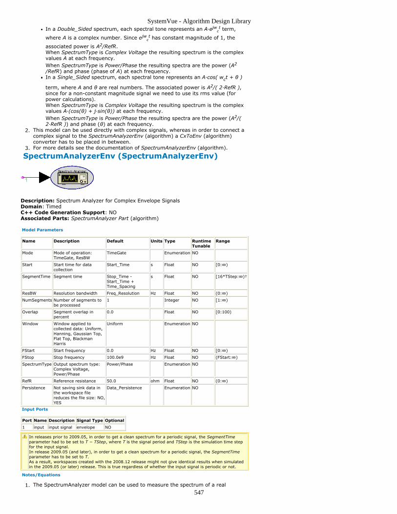
SystemVue - Algorithm Design Library
547
In a Double_Sided spectrum, each spectral tone represents an A·ejwct term,
where A is a complex number. Since ejwct has constant magnitude of 1, the
associated power is A2/RefR.When SpectrumType is Complex Voltage the resulting spectrum is the complexvalues A at each frequency.When SpectrumType is Power/Phase the resulting spectra are the power (A2
/RefR) and phase (phase of A) at each frequency.In a Single_Sided spectrum, each spectral tone represents an A·cos( wct + θ )
term, where A and θ are real numbers. The associated power is A2/( 2·RefR ),since for a non-constant magnitude signal we need to use its rms value (forpower calculations).When SpectrumType is Complex Voltage the resulting spectrum is the complexvalues A·(cos(θ) + j·sin(θ)) at each frequency.When SpectrumType is Power/Phase the resulting spectra are the power (A2/(2·RefR )) and phase (θ) at each frequency.
This model can be used directly with complex signals, whereas in order to connect a2.complex signal to the SpectrumAnalyzerEnv (algorithm) a CxToEnv (algorithm)converter has to be placed in between.For more details see the documentation of SpectrumAnalyzerEnv (algorithm).3.
SpectrumAnalyzerEnv (SpectrumAnalyzerEnv)
Description: Spectrum Analyzer for Complex Envelope SignalsDomain: TimedC++ Code Generation Support: NOAssociated Parts: SpectrumAnalyzer Part (algorithm)
Model Parameters
Name Description Default Units Type RuntimeTunable
Range
Mode Mode of operation:TimeGate, ResBW
TimeGate Enumeration NO
Start Start time for datacollection
Start_Time s Float NO [0:∞)
SegmentTime Segment time Stop_Time -Start_Time +Time_Spacing
s Float NO [16*TStep:∞)†
ResBW Resolution bandwidth Freq_Resolution Hz Float NO (0:∞)
NumSegments Number of segments tobe processed
1 Integer NO [1:∞)
Overlap Segment overlap inpercent
0.0 Float NO [0:100)
Window Window applied tocollected data: Uniform,Hanning, Gaussian Top,Flat Top, BlackmanHarris
Uniform Enumeration NO
FStart Start frequency 0.0 Hz Float NO [0:∞)
FStop Stop frequency 100.0e9 Hz Float NO (FStart:∞)
SpectrumType Output spectrum type:Complex Voltage,Power/Phase
Power/Phase Enumeration NO
RefR Reference resistance 50.0 ohm Float NO (0:∞)
Persistence Not saving sink data inthe workspace filereduces the file size: NO,YES
Data_Persistence Enumeration NO
Input Ports
Port Name Description Signal Type Optional
1 input input signal envelope NO
In releases prior to 2009.05, in order to get a clean spectrum for a periodic signal, the SegmentTimeparameter had to be set to T − TStep, where T is the signal period and TStep is the simulation time stepfor the input signal.In release 2009.05 (and later), in order to get a clean spectrum for a periodic signal, the SegmentTimeparameter has to be set to T.As a result, workspaces created with the 2008.12 release might not give identical results when simulatedin the 2009.05 (or later) release. This is true regardless of whether the input signal is periodic or not.
Notes/Equations
The SpectrumAnalyzer model can be used to measure the spectrum of a real1.

SystemVue - Algorithm Design Library
548
baseband or a complex envelope signal. In the following notes TStep is used todenote the simulation time step and fc is used to denote the signal characterizationfrequency (fc = 0 for a real baseband signal and fc>0 for a complex envelope signal).The SpectrumAnalyzer has two modes of operation: TimeGate and ResBW. The mode2.of operation is selected in the Mode parameter.In both modes of operation the model collects data starting at Start and untilNumSegments segments that overlap by Overlap% are collected. Each segment iswindowed by the specified Window, the spectrum of each segment is computed, andfinally the spectra are averaged. The only difference between the two modes ofoperation is that
in TimeGate mode, the duration of each segment is SegmentTime.in ResBW mode, the duration of each segment is NENBW/ResBW, where NENBWis the the Normalized Equivalent Noise Bandwidth of the window used.
The spectrum of a basedband signal extends from 0 Hz to 1/(2 × TStep) Hz. The3.spectrum of an RF signal extends from fc − 1/(2 × TStep) Hz to fc + 1/(2 × TStep)Hz. When fc < 1/(2 × TStep), the spectrum extends to negative frequencies. Thespectral content at these negative frequencies is conjugated, mirrored, and added tothe spectral content of the closest positive frequency. This way, the negativefrequency tones are displayed on the positive frequency axis as would happen in areal spectrum analyzer measurement instrument. This process can introduce an errorin the displayed frequency for the mirrored tones. The absolute error introduced isless than Δf/2, where Δf is 1/SegmentTime (in TimeGate mode) and ResBW/NENBW(in ResBW mode). The FStart and FStop parameters are used to control thefrequencey range over which the spectrum will be calculated. If FStart and Fstop areoutside the limits mentioned above they are reset to the lower and higher limitsrespectively.The SpectrumType parameter is used to select the type of spectrum to be computed.4.The computed spectrum is always a Single Sided spectrum. See SpectrumAnalyzerCx(algorithm) for details regarding Single Sided and Double Sided spectra and theinterpretation of Complex Voltage and Power/Phase spectra.
If SpectrumType is Complex Voltage, then the computed spectrum is thecomplex amplitude voltage spectrum. The result is saved in the dataset in acomplex variable named <InstanceName>, where <InstanceName> is themodel's instance name.If SpectrumType is Power/Phase, then there are two spectra computed: thepower spectrum and the phase spectrum. The results are saved in the dataset intwo real variables named <InstanceName>_Power and<InstanceName>_Phase, where <InstanceName> is the model's instance name.
Windowing in spectral analysis and how to choose the right window5.
Windowing is necessary in transform-based (FFT) spectrum estimation. Withoutwindowing, the estimated spectrum can suffer from spectral leakage that can causemisleading measurements or masking of weak signal spectral detail by spuriousartifacts.Every time a window is applied to a signal, leakage occurs, that is, power from onespectral component leaks into the adjacent ones. Leakage from strong spectralcomponents can result in hiding/masking of nearby weaker spectral components.Even strong spectral components can be affected by leakage. For example, twostrong spectral components close to each other can appear as one due to leakage.Choosing the right window for a spectral measurement is very important. The choiceof window depends on what is being measured and what the trade-offs betweenfrequency resolution (ability to distinguish spectral components of comparablestrength that are close to each other) and dynamic range (ability to measure signalswith spectral components of widely varying strengths and distributed over a widerange) are.Windows can be characterized by their Normalized Equivalent Nosie BandWidth(NENBW). Equivalent Noise Bandwidth (ENBW) compares a window to an ideal,rectangular filter. It is the equivalent width of a rectangular filter that passes thesame amount of white noise as the window. The Normalized ENBW (NENBW) is theENBW multiplied by the time duration of the signal being windowed. In general, forthe same length of signal processed, the higher the NENBW of a window the higherits dynamic range (less leakage) and the poorer its frequency resolution. The NENBWof the windows available in the SpectrumAnalyzer is given in the table below:
Window NENBW
Uniform 1
Hanning 1.5
Gaussian Top 2.215
Flat Top 3.819
Blackman Harris 2.021
Some general guidelines for choosing a window are given below:
Do not use a window (set Window to Uniform) when analyzing transients.For periodic signals whose spectral components have comparable strengths andwhen the signal segment processed includes an exact integer multiple ofperiods, the best results are obtained if no window is used (set Window toUniform). Any start up transients should be excluded.

SystemVue - Algorithm Design Library
549
For periodic signals whose spectral components have significantly differentstrengths and/or when the signal segment processed does not include an exactinteger multiple of periods, the use of a window can improve the detection ofthe weaker spectral components. The higher the NENBW the more likely theweaker spectral components will be detected. However, this trades-offfrequency resolution and so if the spectral components are very close to eachother the weaker one might remain unresolved. To improve frequency resolutionwhile still maintaining a good dynamic range use a window but process a longersignal segment.For aperiodic signals such as modulated signals (QPSK, QAM, GSM, EDGE,CDMA, OFDM) the use of a window is highly recommended. The window willattenuate the signal at both ends of the signal segment processed to zero. Thismakes the signal apear periodic and reduces leakage.
The definitions of the windows available in the SpectrumAnalyzer model are given6.below (N is the length of the window in number of samples):
References
A. V. Oppenheim, R. W. Schafer, Discrete-Time Signal Processing, Prentice Hall,1.1989, Chapter 9, section 9.7.

SystemVue - Algorithm Design Library
550
WriteBaseBandStudioFile PartCategories: Sinks (algorithm)
The models associated with this part are listed below. To view detailed information on amodel (description, parameters, equations, notes, etc.), please click the appropriate link.
Model Description
WriteBaseBandStudioFile (algorithm) Base Band Studio Formatted File Writer
WriteBaseBandStudioFileNormalize(algorithm)
Base Band Studio Formatted File Writer with InputNormalization
WriteBaseBandStudioFile
Description: Base Band Studio Formatted File WriterDomain: TimedC++ Code Generation Support: NOAssociated Parts: WriteBaseBandStudioFile Part (algorithm)
Model Parameters
Name Description Default Units Type RuntimeTunable
Range Symbol
File Input file name file.bin Filename NO F
StartStopOption Sink collectionmode: Auto,Samples, Time
Auto Enumeration NO
SampleStart Sample numberto start datacollection
0 Integer NO [0:∞)
SampleStop Sample numberto stop datacollection
Num_Samples- 1
Integer NO [SampleStart:∞)
TimeStart Time to start datacollection
Start_Time s Float NO [0:∞)
TimeStop Time to stop datacollection
Stop_Time s Float NO [TimeStart:∞)
Input Ports
Port Name Description Signal Type Optional
1 IQ IQ data complex NO
2 Marker14R Real Bit 14 Marker int YES
3 Marker14I Imag Bit 14 Marker int YES
4 Marker15R Real Bit 15 Marker int YES
5 Marker15I Imag Bit 15 Marker int YES
Notes/Equations
Write IQ complex data and boolean markers in the Base Band Studio format to a file1.named by the File parameter.Each Base Band Studio sample consists of a pair of 16 bit signed integers which2.encode the IQ and up to 4 marker values. The first integer hold the real parts whilethe second integer hold the imaginary parts.If Marker14R or Marker14I is connected, the IQ will have 14 bit quantization. If only3.Marker15R or Marker15I is connected, then the IQ will have 15 bit quantization.Otherwise, the IQ will have 16 bit quantization.The IQ input is a complex value with the I value in the imaginary part and the Q4.value in the real part. If the input is outside the range [-1, 1), the value is clipped tothis range before quantization.A marker input is resolved to a zero bit, only if the marker input is zero. The marker5.bits occupy the least significant bits (LSB) of both integers. The marker name, e.g.Marker15R, indicate which bit and which integer hold the bit value, e.g. Marker15Rstates the LSB (15) of the first integer (R) is used store Marker15R. The next greaterLSB is bit 14.A Browse button is provided at the lower left corner of the properties window to6.provide a relative path for File. This path is relative to the folder from which theworkspace is loaded. If an absolute path is desired, directly enter the full path intothe Value column.

SystemVue - Algorithm Design Library
551
See Sink (algorithm) for a description of the output control parameters.7.The Base Band Studio format has implementation in ADS and is used in Agilent8.instrumentation. For more information, see CM BB StudioStreamWrite .
Important Links
Learn more about Baseband Studio from Agilent Technologies1.Also see the following related parts:2.ReadBaseBandStudioFile (algorithm)WriteBaseBandStudioFileNormalize (algorithm)
WriteBaseBandStudioFileNormalize
Description: Base Band Studio Formatted File WriterDomain: TimedC++ Code Generation Support: NOAssociated Parts: WriteBaseBandStudioFile Part (algorithm)
Model Parameters
Name Description Default Units Type RuntimeTunable
Range Symbol
File Input file name file.bin Filename NO F
StartStopOption Sink collectionmode: Auto,Samples, Time
Auto Enumeration NO
SampleStart Sample numberto start datacollection
0 Integer NO [0:∞)
SampleStop Sample numberto stop datacollection
Num_Samples- 1
Integer NO [SampleStart:∞)
TimeStart Time to start datacollection
Start_Time s Float NO [0:∞)
TimeStop Time to stop datacollection
Stop_Time s Float NO [TimeStart:∞)
Input Ports
Port Name Description Signal Type Optional
1 IQ IQ data complex NO
2 Marker14R Real Bit 14 Marker int YES
3 Marker14I Imag Bit 14 Marker int YES
4 Marker15R Real Bit 15 Marker int YES
5 Marker15I Imag Bit 15 Marker int YES
Notes/Equations
Write IQ complex data and boolean markers in the Base Band Studio format to a file1.named by the File parameter.Each Base Band Studio sample consists of a pair of 16 bit signed integers which2.encode the IQ and up to 4 marker values. The first integer hold the real parts whilethe second integer hold the imaginary parts.If Marker14R or Marker14I is connected, the IQ will have 14 bit quantization. If only3.Marker15R or Marker15I is connected, then the IQ will have 15 bit quantization.Otherwise, the IQ will have 16 bit quantization.The IQ input is a complex value with the I value in the imaginary part and the Q4.value in the real part. The I and Q are normalized to the range [-1, 32767/32768]before quantization. The normalization value is saved to a file whose name is formedby appending ".Normalization.txt" to the File parameter value. The normalization fileis intended for use by ReadBaseBandStudioFile (algorithm).A marker input is resolved to a zero bit, only if the marker input is zero. The marker5.bits occupy the least significant bits (LSB) of both integers. The marker name, e.g.Marker15R, indicate which bit and which integer hold the bit value, e.g. Marker15Rstates the LSB (15) of the first integer (R) is used store Marker15R. The next greaterLSB is bit 14.A Browse button is provided at the lower left corner of the properties window to6.provide a relative path for File. This path is relative to the folder from which theworkspace is loaded. If an absolute path is desired, directly enter the full path intothe Value column.See Sink (algorithm) for a description of the output control parameters.7.

SystemVue - Algorithm Design Library
552
The Base Band Studio format has implementation in ADS and is used in Agilent8.instrumentation. For more information, see CM BB StudioStreamWrite .
Important Links
Learn more about Baseband Studio from Agilent Technologies1.Also see the following related parts:2.ReadBaseBandStudioFile (algorithm)WriteBaseBandStudioFileNormalize (algorithm)

SystemVue - Algorithm Design Library
553
WriteFile PartCategories: Sinks (algorithm)
The models associated with this part are listed below. To view detailed information on amodel (description, parameters, equations, notes, etc.), please click the appropriate link.
Model Description
WriteN6030File(algorithm)
N6030 Formatted File Writer
WriteN6030File
Description: N6030 Formatted File WriterDomain: TimedC++ Code Generation Support: NOAssociated Parts: WriteFile Part (algorithm)
Model Parameters
Name Description Default Units Type RuntimeTunable
Range
StartStopOption Sink collectionmode: Auto,Samples, Time
Auto Enumeration NO
SampleStart Sample number tostart datacollection
0 Integer NO [0:∞)
SampleStop Sample number tostop data collection
Num_Samples- 1
Integer NO [SampleStart:∞)
TimeStart Time to start datacollection
Start_Time s Float NO [0:∞)
TimeStop Time to stop datacollection
Stop_Time s Float NO [TimeStart:∞)
FileI I input file name file_i.bin Filename NO
FileQ Q input file name file_q.bin Filename NO
NormalizeData Normalize data toavoid clipping: NO,YES
YES Enumeration NO
FullScaleFactor Full scale factor forpeak value
1.0 Float NO [0.000030517578125:1]
Input Ports
Port Name Description Signal Type Optional
1 input IQ data complex NO
Notes/Equations
This model writes IQ data into the files FileI and FileQ using the N6030 format. Data1.is recorded as 16 bit signed integers.IQ data is represented as a complex value with the I value in the real part and the Q2.value in the imaginary part.The StartStopOption parameter specifies the data collection mode:3.
if set to Samples the data collection will start at sample SampleStart and stop atSampleStop.if set to Time the data collection will start at time TimeStart and stop atTimeStop.if set to Auto then all of SampleStart, SampleStop, TimeStart, and TimeStopneed to be specified and the model will decide at runtime whether SampleStart/SampleStop or TimeStart/TimeStop will be used. The decision is based onwhether the input signal has a sampling rate defined. If there is no samplingrate defined (e.g. signal coming out of a SineGen (algorithm) source withSampleRateOption set to UnTimed) then SampleStart/SampleStop is used.Otherwise, TimeStart/TimeStop is used.
The FileI and FileQ parameters are used to define the output files for the I and Q4.data. The files can be specified with a full path name or a relative path name.Relative path names are relative to the directory where the workspace is located.The NormalizeData parameter controls whether the data will be clipped or normalized5.before it is written to the files.
if set to NO, no normalization is done. Data values outside the range [-FullScaleFactor, FullScaleFactor] are clipped to the limits of this range. Awarning message is also displayed to make the user aware that clippingoccured.

SystemVue - Algorithm Design Library
554
if set to YES, no clipping is performed and the data written to the files is ascaled (normalized) version of the input data so that it is always in the range [-FullScaleFactor, FullScaleFactor]. The scaling factor used is displayed in aninformation message in the Errors window as well as in the simulation log.
See:ReadN6030File (algorithm)WriteBaseBandStudioFile (algorithm)Sink (algorithm)
Important Links
Learn more about N6030 Arbitrary Waveform Generator from Agilent Technologies1.
SystemVue - Algorithm Design Library
555
Sources About SourcesSources are parts with only outputs, i.e. they provide stimulus to a simulation. Everysimulation must have at least one source.
In addition to data, sources can optionally associate time with each output sample. Toachieve reproducibility, all sources keep time with a 64 bit unsigned integer. The effectivetime step for the source is represented as a unit quantity with 20 bits of fraction allowingfor a precision of 0.95367 10-6 (from 2-20) or approximately 1 ppm. The remaining 44 bitsallow for 1.7592 1013 (from 244 - 1) time steps.
At times, the 64 bit time quantity is converted to a double precision floating point quantitywhich has only 53 bits of precision. Therefore, the internal time resolution can only bemaintained for 8.5899 109 (from 253 - 20 - 1) time steps and degrades slowly to aminimum precision 1.9531 10-3 (from 2-(53 - 44)) of one time step.
All source parameter values that are specified in time are rounded to the nearestrepresentation. Parameters that are specified in frequency have their representation intime as a reciprocal are also rounded to the nearest representation. If a source cannotrepresent a parameter within a 10-6 relative error, an error message is generated and thesimulation is stopped. Choose a higher effective sample rate (lower effective time step) toresolve this error.
For example, a 1 Hz source has a time step of 1 s.
Source time range has range [0, 1.7592 1013) seconds or [0, 4.8867 109) hours or[0, 2.0361 108) days or [0, 5.57 105) years.A time parameter of 1 - 2-21 s is rounded to 1 s and has range [-8.7960 1012, 8.79601012] s.A frequency parameter of 1/(1 - 2-21) Hz is rounded to 1 Hz and has range [5.684410-14, 1.0485 106] Hz.
Sub classes:
Timed Sources (algorithm)Untimed Sources (algorithm)
ContentsBits Part (algorithm)ChirpGen Part (algorithm)ComplexExpGen Part (algorithm)Const Part (algorithm)DataPort Part (algorithm)Diagonal M Part (algorithm)GaussianNoiseGen Part (algorithm)Identity M Part (algorithm)IID Gaussian Part (algorithm)IID Uniform Part (algorithm)Impulse Part (algorithm)NoiseFMask Part (algorithm)Oscillator Part (algorithm)PulseGen Part (algorithm)Ramp Part (algorithm)RampGen Part (algorithm)RampSweepGen Part (algorithm)ReadBaseBandStudioFile Part (algorithm)ReadFile Part (algorithm)SineGen Part (algorithm)SineSweepGen Part (algorithm)SquareGen Part (algorithm)SquareSweepGen Part (algorithm)WalshCode Part (algorithm)WaveForm Part (algorithm)Window Part (algorithm)
About Bit Rate SourcesSuper class:
Untimed Burst Sources (algorithm)
New bit values are generated at frequency, BitRate, while the part is operating at some

SystemVue - Algorithm Design Library
556
sample rate. BitRate cannot exceed the sample rate.
Parameters:
BitRate. Default is from the Data Flow Analysis sample rate.1.
For other parameter descriptions, see Untimed Burst Sources (algorithm).
About File SourcesSuper class:
Untimed Burst Sources (algorithm)
These parts are classified as file readers where samples are read sequentially from File,decoded and output.sfunction = 0 always output the first sample in the file, and so on. For sfunction definition,
see Untimed Burst Sources (algorithm).
Parameters:
File. Default varies by model. A Browse button is provided at the lower left corner of1.the properties window to provide a relative path for File. This path is relative to thefolder from which the workspace is run. If an absolute path is desired, directly enterthe full path into the Value column.Periodic. Default is YES. If YES, the file is reread from the beginning after an end of2.file condition. Otherwise, zeros are output.
For other parameter descriptions, see Untimed Burst Sources (algorithm).
The following table (and plots) summarize the behavior of the file based sources. The plotswere generated using the ReadFile model with a file whose contents were the numbersfrom 1 to 10:
Plot # Periodic BurstMode BurstLength What is output
1 NO OFF Any file content output once followed by zeros
2 YES OFF Any file content output repeatedly
3 NO Single > file content file content zero padded to BurstLength and output once
4 YES Single > file content file content repeated to BurstLength and output once
5 NO orYES
Single = file content file content output once
6 NO orYES
Single < file content file content truncated to BurstLength and output once
7 NO Multiple > file content file content zero padded to BurstLength and output inbursts
8 YES Multiple > file content file content repeated to BurstLength and output in bursts
9 NO orYES
Multiple = file content file content output in bursts
10 NO orYES
Multiple < file content file content truncated to BurstLength and output in bursts
Plot 1
Plot 2

SystemVue - Algorithm Design Library
557
Plot 3
Plot 4
Plot 5
Plot 6

SystemVue - Algorithm Design Library
558
Plot 7
Plot 8
Plot 9
Plot 10

SystemVue - Algorithm Design Library
559
About Time Burst SourcesSuper class:
Timed Sources (algorithm).
These parts have burst mode capability. If burst mode is enabled, the output is defined onone (BurstMode is Single) or more (BurstMode is Multiple) segments of BurstPeriod (BP)seconds. The burst time, tburst, is tsource modulo BP. For tsource definition, see Timed
Sources (algorithm).
A signal format exists within a burst period. There can be a delay of BurstDelay (DB)seconds at the beginning and a signal length of BurstLength (BL) seconds after the delay.A quiescent value that is defined for each part is the output for those times outside of thespecific signal definition, DB ≤ tburst < DB + BL, but within the burst period.
If BurstMode is OFF, the specific signal time tfunction is tsource, otherwise tfunction is tburst -
DB when DB ≤ tburst < DB + BL and unused elsewhere.
Parameters:
BurstMode (B). Default is OFF.1.BurstLength (BL). Default is 100 μs.2.BurstPeriod (BP). Default is 200 μs.3.BurstDelay (DB). Default is 0 μs.4.
For other parameter descriptions, see Timed Sources (algorithm).
The following plots show the output of a SineGen (algorithm) source with Amplitude = 1V, Offset = 0 V, Frequency = 20 kHz, Phase = 0°, and different burst configurations.

SystemVue - Algorithm Design Library
560

SystemVue - Algorithm Design Library
561
About Timed SourcesSuper class:
Sources Category (algorithm)
Sub classes:
Time Burst Sources (algorithm)Time Swept Sources (algorithm)
Parts whose signal generation require a sense of time are members of this class. IfSampleRateOption is Timed from Schematic, then time information comes from the partports, otherwise the SampleRate parameter is used. If SampleRateOption is set toUntimed, the output is simply stripped of time information.
Let tsys be the simulation time which begins at 0 seconds.
Specific signal definition begins at InitialDelay (D) seconds, i.e. tsource ≥ 0 where tsource is
tsys - D. A fill value defines the signal for tsys < D. Typically, a fill value is some form of
zero.
The combined signal is sampled from tsys = 0 at a fixed sample rate (S), i.e. tsys = n / S
for n = 0, 1, 2 ...
Parameters:
ShowAdvancedParameters. Default is NO.1.SampleRateOption (SO). Default is Timed from Schematic.2.SampleRate (S). Default is from the Data Flow Analysis sample rate.3.InitialDelay (D). Default is zero seconds.4.
About Time Swept SourcesSuper class:
Timed Sources (algorithm)
These sources are defined by an instantaneous frequency Fi(tsweep), which is swept from
StartFreq (F1) to StopFreq (F2) in a SweepPeriod (SP) time interval. The sweep time t
sweep, is defined as tsource modulo SP. For tsource definition, see Timed Sources
(algorithm).
The instantaneous frequency Fi(tsweep) is:
Fi(tsweep) = F1 + (F2 - F1)·(tsweep / SP), if FSweepType is linear.
Fi(tsweep) = F1·(F2/F1)tsweep/SP, if FSweepType is log (Fi(tsweep) is swept linearly in a
log scale).
Parameters:
FSweepType (FT). Default is linear.1.StartFreq (F1). Default is 1 KHz.2.StopFreq (F2). Default is 10 KHz.3.SweepPeriod (SP). Default is set from the data flow analysis field, Stop Time, thus4.enabling a single sweep.
For other parameter descriptions, see Timed Sources (algorithm).
About Untimed Burst Sources

SystemVue - Algorithm Design Library
562
Super class:
Untimed Sources (algorithm)
Sub classes:
Bit Rate Sources (algorithm)File Sources (algorithm)
These parts have burst mode capability. If burst mode is enabled, the output is defined onone (BurstMode is Single) or more (BurstMode is Multiple) BurstPeriod (BP) samplesegments. The burst sample number, sburst, is ssource modulo BP. For ssource definition,
see Untimed Sources (algorithm).
A signal format exists within a burst period. There can be a delay of BurstDelay (DB)samples at the beginning and a signal length of BurstLength (BL) samples after the delay.A quiescent value that is defined for each part is the output for those sample numbersoutside of the specific signal definition, DB ≤ sburst < DB + BL, but within the burst period.
If BurstMode is OFF, the specific signal sample number sfunction is ssource, otherwise s
function is sburst - DB when DB ≤ sburst < DB + BL and unused elsewhere.
Parameters:
BurstMode. Default is OFF.1.BurstLength (BL). Default is 100 samples.2.BurstPeriod (BP). Default is 200 samples.3.BurstDelay (DB). Default is 0 samples.4.
For other parameter descriptions, see Untimed Sources (algorithm).
About Untimed SourcesSuper class:
Sources Category (algorithm)
Sub classes:
Untimed Burst Sources (algorithm)
Parts whose signal generation is defined only on sample numbers are members of thisclass. Time information can be associated with the output, if SampleRateOption is Timedfrom Schematic when time information comes from the part ports, or if SampleRateOptionis Timed from SampleRate when the SampleRate parameter is used.
Let ssys be the simulation sample number which begins at 0.
Specific signal definition begins at InitialDelay (D) samples, i.e. ssource ≥ 0 where ssource is
ssys - D. A fill value defines the signal for ssys < D. Typically, a fill value is some form of
zero.
Parameters:
ShowAdvancedParameters. Default is NO.1.SampleRateOption (SO). Default is Timed from Schematic.2.SampleRate (S). Default is from the Data Flow Analysis sample rate.3.InitialDelay (D). Default is 0 sample delays.4.

SystemVue - Algorithm Design Library
563
Bits PartCategories: Sources (algorithm)
The models associated with this part are listed below. To view detailed information on amodel (description, parameters, equations, notes, etc.), please click the appropriate link.
Model Description
RandomBits(algorithm)
Random Bit Generator
DataPattern(algorithm)
Patterned Data Source
PRBS (algorithm) Pseudo Random Binary Sequence Generator
DataPattern (Patterned Data Source)
Description: Patterned Data SourceDomain: TimedC++ Code Generation Support: NOAssociated Parts: Bits Part (algorithm)
Model Parameters
Name Description Default Units Type RuntimeTunable
Range Symbol
DataPattern Data pattern:PN9, PN15,FIX4,_4_1_4_0,_8_1_8_0,_16_1_16_0,_32_1_32_0,_64_1_64_0
PN9 Enumeration YES T
BitRate Output bit rate Sample_Rate Hz Float NO [0:SampleRate]
ShowAdvancedParams Show advancedparameters:NO, YES
NO Enumeration NO
SampleRateOption Sample rateoption:UnTimed,Timed fromSampleRate,Timed fromSchematic
Timed fromSchematic
Enumeration NO SO
SampleRate Explicit samplerate
Sample_Rate Hz Float NO ( 0:∞ ) S
InitialDelay Output sampledelay
0 Integer YES [ 0:∞ ) D
BurstMode Burst mode:OFF, Single,Multiple
OFF Enumeration YES
BurstLength Burst samplelength
100 Integer YES [1:∞) BL
BurstPeriod Samples fromstart of oneburst to start ofnext
200 Integer YES [1:∞) BP
BurstDelay Sample delaywithin burstbefore the startof the burstlength interval
0 Integer YES [0:BurstPeriod-BurstLength]
DB
Output Ports
Port Name Signal Type Optional
1 output boolean NO
Notes/Equations
This model generates one of eight specific bit patterns.1.
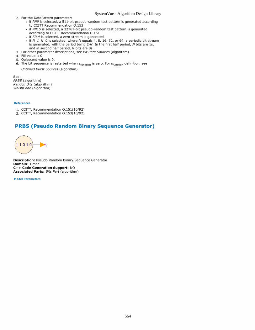
SystemVue - Algorithm Design Library
564
For the DataPattern parameter:2.if PN9 is selected, a 511-bit pseudo-random test pattern is generated accordingto CCITT Recommendation O.153if PN15 is selected, a 32767-bit pseudo-random test pattern is generatedaccording to CCITT Recommendation O.151if FIX4 is selected, a zero-stream is generatedif N_1_N_0 is selected, where N equals 4, 8, 16, 32, or 64, a periodic bit streamis generated, with the period being 2·N. In the first half period, N bits are 1s,and in second half period, N bits are 0s.
For other parameter descriptions, see Bit Rate Sources (algorithm).3.Fill value is 0.4.Quiescent value is 0.5.The bit sequence is restarted when sfunction is zero. For sfunction definition, see6.
Untimed Burst Sources (algorithm).
See:PRBS (algorithm)RandomBits (algorithm)WalshCode (algorithm)
References
CCITT, Recommendation O.151(10/92).1.CCITT, Recommendation O.153(10/92).2.
PRBS (Pseudo Random Binary Sequence Generator)
Description: Pseudo Random Binary Sequence GeneratorDomain: TimedC++ Code Generation Support: NOAssociated Parts: Bits Part (algorithm)
Model Parameters

SystemVue - Algorithm Design Library
565
Name Description Default Units Type RuntimeTunable
Range Symbol
LFSR_Length Linearfeedbackshift registerlength
12 Integer YES [2:31] L
LFSR_InitState Linearfeedbackshift registerinitial state
1 Integer YES [1:2<sup>L</sup>-1]
IS
BitRate Output bitrate
Sample_Rate Hz Float NO [0:SampleRate]
ShowAdvancedParams Showadvancedparameters:NO, YES
NO Enumeration NO
SampleRateOption Sample rateoption:UnTimed,Timed fromSampleRate,Timed fromSchematic
Timed fromSchematic
Enumeration NO SO
SampleRate Explicitsample rate
Sample_Rate Hz Float NO ( 0:∞ ) S
InitialDelay Outputsampledelay
0 Integer YES [ 0:∞ ) D
BurstMode Burst mode:OFF, Single,Multiple
OFF Enumeration YES
BurstLength Burstsamplelength
100 Integer YES [1:∞) BL
BurstPeriod Samplesfrom start ofone burst tostart of next
200 Integer YES [1:∞) BP
BurstDelay Sampledelay withinburst beforethe start ofthe burstlengthinterval
0 Integer YES [0:BurstPeriod-BurstLength]
DB
Output Ports
Port Name Signal Type Optional
1 output boolean NO
Notes/Equations
PRBS generates a pseudo-random bit sequence, using a linear feedback shift register1.(LFSR).The LFSR_Length parameter sets the length of the LFSR as well as selects a2.maximal-length shift-register code with periodicity 2LFSR_Length − 1.The LFSR_InitState parameter sets the initial state of the LFSR. Different3.LFSR_InitState values will generate uncorrelated sequences.For other parameter descriptions, see Bit Rate Sources (algorithm).4.Fill value is 0.5.Quiescent value is 0.6.The bit sequence is restarted when sfunction is zero. For sfunction definition, see7.
Untimed Burst Sources (algorithm).
See:LFSR (algorithm)DataPattern (algorithm)RandomBits (algorithm)WalshCode (algorithm)
RandomBits (Random Bit Generator)

SystemVue - Algorithm Design Library
566
Description: Random Bit GeneratorDomain: TimedC++ Code Generation Support: NOAssociated Parts: Bits Part (algorithm)
Model Parameters
Name Description Default Units Type RuntimeTunable
Range Symbol
ProbOfZero Probability ofzero bit value
0.5 Float YES [0:1] P
BitRate Output bit rate Sample_Rate Hz Float NO [0:SampleRate]
ShowAdvancedParams Showadvancedparameters:NO, YES
NO Enumeration NO
SampleRateOption Sample rateoption:UnTimed,Timed fromSampleRate,Timed fromSchematic
Timed fromSchematic
Enumeration NO SO
SampleRate Explicit samplerate
Sample_Rate Hz Float NO ( 0:∞ ) S
InitialDelay Output sampledelay
0 Integer YES [ 0:∞ ) D
BurstMode Burst mode:OFF, Single,Multiple
OFF Enumeration YES
BurstLength Burst samplelength
100 Integer YES [1:∞) BL
BurstPeriod Samples fromstart of oneburst to startof next
200 Integer YES [1:∞) BP
BurstDelay Sample delaywithin burstbefore thestart of theburst lengthinterval
0 Integer YES [0:BurstPeriod-BurstLength]
DB
Output Ports
Port Name Signal Type Optional
1 output boolean NO
Notes/Equations
This model generates a random bit sequence, in which the probability of a 0 bit is1.ProbOfZero and the probability of a 1 bit is 1 - ProbOfZero.For other parameter descriptions, see Bit Rate Sources (algorithm).2.Fill value is 0.3.Quiescent value is 0.4.The repeatability of the bit sequence generated by this model can be controlled by5.the Repeatable Random Sequences check box in the Option tab of the DF Analysisdialog (sim).
See:LFSR (algorithm)DataPattern (algorithm)PRBS (algorithm)WalshCode (algorithm)

SystemVue - Algorithm Design Library
567
ChirpGen PartCategories: Sources (algorithm)
The models associated with this part are listed below. To view detailed information on amodel (description, parameters, equations, notes, etc.), please click the appropriate link.
Model Description
ChirpGen(algorithm)
Frequency ChirpGenerator
ChirpGen
Description: Frequency Chirp GeneratorDomain: TimedC++ Code Generation Support: NOAssociated Parts: ChirpGen Part (algorithm)
Model Parameters
Name Description Default Units Type RuntimeTunable
Range Symbol
Amplitude Peak sinewavevoltageamplitude
1 V Float YES (-∞:∞) A
Offset DC offsetvoltage
0 V Float YES (-∞:∞) DC
StartFreq Startfrequency
1e3 Hz Float YES (0:SampleRate/4] F1
StopFreq Stopfrequency
10e3 Hz Float YES (0:SampleRate/4] F2
Phase Phase 0 deg Float YES (-∞:∞) PH
SweepPeriod Time periodto completea sweep
Stop_Time +Time_Spacing
s Float YES [1/SampleRate:∞) SP
ShowAdvancedParams Showadvancedparameters:NO, YES
NO Enumeration NO
SampleRateOption Sample rateoption:UnTimed,Timed fromSampleRate,Timed fromSchematic
Timed fromSchematic
Enumeration NO SO
SampleRate Explicitsample rate
Sample_Rate Hz Float NO (0:∞) S
InitialDelay Initialoutput timedelay
0 s Float YES [0:∞) D
Output Ports
Port Name Signal Type Optional
1 output real NO
2 frequency real NO
Notes/Equations
Let Fi(tsweep) be the instantaneous sweep frequency defined in Time Swept Sources1.
(algorithm) and
The ChirpGen model outputs a sinusoidal waveform of the form A·sin(2π·F(tsweep)·t2.
sweep + PH / 360) + DC.
The only difference between this model and SineSweepGen (algorithm) is that this3.model supports only a linear frequency sweep.Fi(tsweep) is output at the frequency port in Hertz.4.
For other parameter descriptions, see Time Swept Sources (algorithm).5.Fill value is 0.6.

SystemVue - Algorithm Design Library
568
See:ComplexExpGen (algorithm)SineGen (algorithm)RampSweepGen (algorithm)SineSweepGen (algorithm)SquareSweepGen (algorithm)

SystemVue - Algorithm Design Library
569
ComplexExpGen PartCategories: Sources (algorithm)
The models associated with this part are listed below. To view detailed information on amodel (description, parameters, equations, notes, etc.), please click the appropriate link.
Model Description
ComplexExpGen(algorithm)
Complex ExponentialSource
ComplexExpGen (Complex Exponential Source)
Description: Complex Exponential SourceDomain: TimedC++ Code Generation Support: NOAssociated Parts: ComplexExpGen Part (algorithm)
Model Parameters
Name Description Default Units Type RuntimeTunable
Range Symbol
Amplitude Peak sinewavevoltageamplitude
1 V Float YES ( -∞:∞ ) A
Offset DC offsetcomplexvoltage
0 V Complexnumber
YES DC
Frequency Frequency 5e3 Hz Float YES [ -SampleRate/2:SampleRate/2]
F
Phase Phase 0 deg Float YES ( -∞:∞ ) PH
QuadraturePolarity Quadraturepolarity:normal,inverted
normal Enumeration YES QP
ShowAdvancedParams Showadvancedparameters:NO, YES
NO Enumeration NO
SampleRateOption Sample rateoption:UnTimed,Timed fromSampleRate,Timed fromSchematic
Timed fromSchematic
Enumeration NO SO
SampleRate Explicitsample rate
Sample_Rate Hz Float NO (0:∞) S
InitialDelay Initialoutput timedelay
0 s Float YES [0:∞) D
BurstMode Burst mode:OFF, Single,Multiple
OFF Enumeration YES B
BurstLength Burst timelength
100e-6 s Float YES [1/SampleRate:∞) BL
BurstPeriod Time periodfrom start ofone burst tostart of next
200e-6 s Float YES [1/SampleRate:∞) BP
BurstDelay Time delaywithin burstbefore thestart of theBurstLengthinterval
0 s Float YES [0:BurstPeriod-BurstLength] DB
Output Ports

SystemVue - Algorithm Design Library
570
Port Name Signal Type Optional
1 output complex NO
Notes/Equations
The function, A·eQ·(2·π·F·tfunction
+ PH / 360) + DC, is output. Q is j for normal1.Quadrature Polarity, otherwise Q is -j. For tfunction definition, see Time Burst Sources
(algorithm).For other parameter descriptions, see Time Burst Sources (algorithm).2.Fill value is 0.3.Quiescent value is DC.4.
See:SineGen (algorithm)SineSweepGen (algorithm)Oscillator (algorithm)

SystemVue - Algorithm Design Library
571
Const PartCategories: C++ Code Generation (algorithm), Sources (algorithm)
The models associated with this part are listed below. To view detailed information on amodel (description, parameters, equations, notes, etc.), please click the appropriate link.
Model Description
Const (algorithm) Constant Generator
ConstFxp(hardware)
Fixed Point Constant
Const (Constant Generator)
Description: Constant GeneratorDomain: TimedC++ Code Generation Support: YES (see Note)Associated Parts: Const Part (algorithm)
Model Parameters
Name Description Default Units Type RuntimeTunable
Range Symbol
Value Value 0 None YES V
ShowAdvancedParams Show advancedparameters: NO, YES
NO Enumeration NO
SampleRateOption Sample rate option:UnTimed, Timed fromSampleRate, Timedfrom Schematic
Timed fromSchematic
Enumeration NO SO
SampleRate Explicit sample rate Sample_Rate Hz Float NO ( 0:∞)
S
InitialDelay Output sample delay 0 Integer YES [ 0:∞)
D
Output Ports
Port Name Signal Type Optional
1 output anytype NO
NoteThis model does not support C++ code generation if the port type is resolved to variant (sim) or ifSampleRateOption is NOT set to UnTimed.
Notes/Equations
Output a constant signal with value given by the Value parameter. For discussion on1.the variant type, see Variant (sim).For other parameter descriptions, see Untimed Sources (algorithm).2.Fill value is 0.3.
See:Identity_M (algorithm)IdentityCx_M (algorithm)Diagonal_M (algorithm)DiagonalCx_M (algorithm)

SystemVue - Algorithm Design Library
572
Diagonal_M PartCategories: Sources (algorithm)
The models associated with this part are listed below. To view detailed information on amodel (description, parameters, equations, notes, etc.), please click the appropriate link.
Model Description
Diagonal_M (algorithm) Diagonal Matrix Generator
DiagonalCx_M(algorithm)
Output matrix diagonalelements
Diagonal_M (Diagonal Matrix Generator)
Description: Diagonal Matrix GeneratorDomain: TimedC++ Code Generation Support: NOAssociated Parts: Diagonal M Part (algorithm)
Model Parameters
Name Description Default Units Type RuntimeTunable
Range Symbol
DiagonalElements Output matrixdiagonal elements
[1, 2] Floating pointarray
NO E
ShowAdvancedParams Show advancedparameters: NO, YES
NO Enumeration NO
SampleRateOption Sample rate option:UnTimed, Timed fromSampleRate, Timedfrom Schematic
Timed fromSchematic
Enumeration NO SO
SampleRate Explicit sample rate Sample_Rate Hz Float NO ( 0:∞)
S
InitialDelay Output sample delay 0 Integer YES [ 0:∞)
D
Output Ports
Port Name Signal Type Optional
1 output real matrix NO
Notes/Equations
Diagonal_M is a constant square matrix source whose dimensions are specified by1.the RowsCols parameter.The constant matrix is formed by inserting values from the real DiagonalElements2.array parameter into the diagonal elements beginning at element [1,1]. Zeroes areinserted at the off diagonal elements.The number of elements in DiagonalElements must be at least RowCols.3.For other parameter descriptions, see Untimed Sources (algorithm).4.Fill value is a real matrix zero.5.
See:DiagonalCx_M (algorithm)Identity_M (algorithm)IdentityCx_M (algorithm)Const (algorithm)
DiagonalCx_M (Output matrix diagonal elements)
Description: Output matrix diagonal elementsDomain: TimedC++ Code Generation Support: NOAssociated Parts: Diagonal M Part (algorithm)
Model Parameters

SystemVue - Algorithm Design Library
573
Name Description Default Units Type RuntimeTunable
Range Symbol
DiagonalElements Output matrixdiagonal elements
[1, j] Complexarray
NO E
ShowAdvancedParams Show advancedparameters: NO, YES
NO Enumeration NO
SampleRateOption Sample rate option:UnTimed, Timed fromSampleRate, Timedfrom Schematic
Timed fromSchematic
Enumeration NO SO
SampleRate Explicit sample rate Sample_Rate Hz Float NO ( 0:∞)
S
InitialDelay Output sample delay 0 Integer YES [ 0:∞)
D
Output Ports
Port Name Signal Type Optional
1 output complex matrix NO
Notes/Equations
DiagonalCx_M is a constant square matrix source whose dimensions are specified by1.the RowsCols parameter.The constant matrix is formed by inserting values from the complex2.DiagonalElements array parameter into the diagonal elements beginning at element[1,1]. Zeroes are inserted at the off diagonal elements.The number of elements in DiagonalElements must be at least RowCols.3.For other parameter descriptions, see Untimed Sources (algorithm).4.Fill value is a complex matrix zero.5.
See:Diagonal_M (algorithm)Identity_M (algorithm)IdentityCx_M (algorithm)Const (algorithm)

SystemVue - Algorithm Design Library
574
GaussianNoiseGen PartCategories: Sources (algorithm)
The models associated with this part are listed below. To view detailed information on amodel (description, parameters, equations, notes, etc.), please click the appropriate link.
Model Description
GaussianNoiseGen(algorithm)
Gaussian NoiseGenerator
GaussianNoiseGen (Gaussian Noise Generator)
Description: Gaussian Noise GeneratorDomain: TimedC++ Code Generation Support: NOAssociated Parts: GaussianNoiseGen Part (algorithm)
Model Parameters
Name Description Default Units Type RuntimeTunable
Range Symbol
NDensity Noise powerspectraldensity
4.00388587e-21
W Float YES [0:∞) ND
RefR Referenceresistance
50 ohm Float NO (0:∞)
ShowAdvancedParams Showadvancedparameters:NO, YES
NO Enumeration NO
SampleRateOption Sample rateoption:UnTimed,Timed fromSampleRate,Timed fromSchematic
Timed fromSchematic
Enumeration NO SO
SampleRate Explicitsample rate
Sample_Rate Hz Float NO (0:∞) S
InitialDelay Initialoutput timedelay
0 s Float YES [0:∞) D
BurstMode Burst mode:OFF, Single,Multiple
OFF Enumeration YES B
BurstLength Burst timelength
100e-6 s Float YES [1/SampleRate:∞) BL
BurstPeriod Time periodfrom start ofone burst tostart of next
200e-6 s Float YES [1/SampleRate:∞) BP
BurstDelay Time delaywithin burstbefore thestart of theBurstLengthinterval
0 s Float YES [0:BurstPeriod-BurstLength]
DB
Output Ports
Port Name Signal Type Optional
1 output real NO
Notes/Equations
Output additive white Gaussian noise (AWGN) that is characterized by the NDensity1.parameter over the bandwidth specified by the SampleRate parameter into RefRohms.The Gaussian noise has zero mean and standard deviation of2.
.NDensity is the noise density in Watts/Hz and is related to temperature T in Kelvin as3.k·T where k is the Boltzmann constant (1.3806504e-23). At the standard systemtemperature of 290 Kelvin (16.85 Celsius), the NDensity is 4.00388587e-21 Watts/Hz(-173.975 dBm/Hz).For other parameter descriptions, see Time Burst Sources (algorithm).4.

SystemVue - Algorithm Design Library
575
Fill value is 0.5.Quiescent value is 0.6.
See:IID_Gaussian (algorithm)IID_Uniform (algorithm)

SystemVue - Algorithm Design Library
576
IID_Gaussian PartCategories: Sources (algorithm)
The models associated with this part are listed below. To view detailed information on amodel (description, parameters, equations, notes, etc.), please click the appropriate link.
Model Description
IID_Gaussian(algorithm)
IID Gaussian Noise Waveform
IID_Gaussian (IID Gaussian Noise Waveform)
Description: IID Gaussian Noise WaveformDomain: TimedC++ Code Generation Support: NOAssociated Parts: IID Gaussian Part (algorithm)
Model Parameters
Name Description Default Units Type RuntimeTunable
Range Symbol
StdDev Standarddeviation
1 V Float YES (-∞:∞) SD
Offset Offset value 0 V Float YES (-∞:∞) O
ShowAdvancedParams Show advancedparameters:NO, YES
NO Enumeration NO
SampleRateOption Sample rateoption:UnTimed,Timed fromSampleRate,Timed fromSchematic
Timed fromSchematic
Enumeration NO SO
SampleRate Explicit samplerate
Sample_Rate Hz Float NO ( 0:∞ ) S
InitialDelay Output sampledelay
0 Integer YES [ 0:∞ ) D
BurstMode Burst mode:OFF, Single,Multiple
OFF Enumeration YES
BurstLength Burst samplelength
100 Integer YES [1:∞) BL
BurstPeriod Samples fromstart of oneburst to start ofnext
200 Integer YES [1:∞) BP
BurstDelay Sample delaywithin burstbefore the startof the burstlength interval
0 Integer YES [0:BurstPeriod-BurstLength]
DB
Output Ports
Port Name Signal Type Optional
1 output real NO
Notes/Equations
Identically independently distributed variates with Gaussian distribution as specified1.by mean from the Offset parameter and standard deviation from the StdDevparameter are output. The output is commonly referenced as additive white Gaussiannoise (AWGN).For other parameter descriptions, see Untimed Burst Sources (algorithm).2.Fill value is 0.3.Quiescent value is 0.4.
See:IID_Uniform (algorithm)GaussianNoiseGen (algorithm)
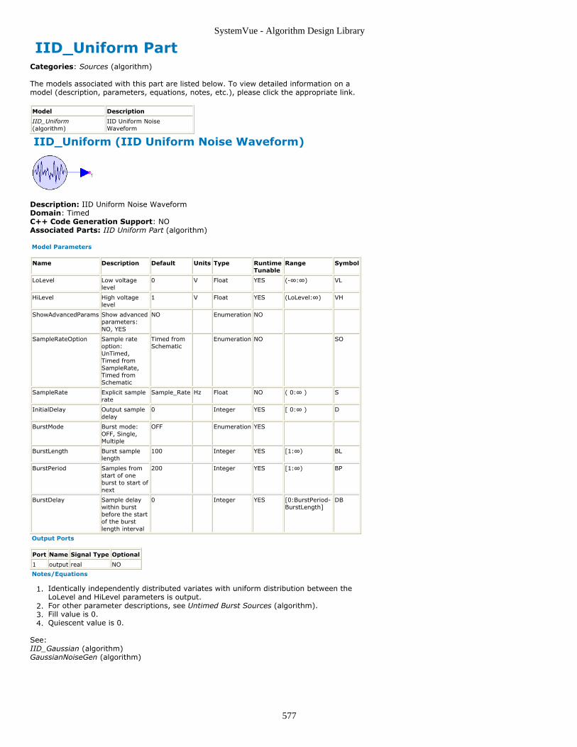
SystemVue - Algorithm Design Library
577
IID_Uniform PartCategories: Sources (algorithm)
The models associated with this part are listed below. To view detailed information on amodel (description, parameters, equations, notes, etc.), please click the appropriate link.
Model Description
IID_Uniform(algorithm)
IID Uniform NoiseWaveform
IID_Uniform (IID Uniform Noise Waveform)
Description: IID Uniform Noise WaveformDomain: TimedC++ Code Generation Support: NOAssociated Parts: IID Uniform Part (algorithm)
Model Parameters
Name Description Default Units Type RuntimeTunable
Range Symbol
LoLevel Low voltagelevel
0 V Float YES (-∞:∞) VL
HiLevel High voltagelevel
1 V Float YES (LoLevel:∞) VH
ShowAdvancedParams Show advancedparameters:NO, YES
NO Enumeration NO
SampleRateOption Sample rateoption:UnTimed,Timed fromSampleRate,Timed fromSchematic
Timed fromSchematic
Enumeration NO SO
SampleRate Explicit samplerate
Sample_Rate Hz Float NO ( 0:∞ ) S
InitialDelay Output sampledelay
0 Integer YES [ 0:∞ ) D
BurstMode Burst mode:OFF, Single,Multiple
OFF Enumeration YES
BurstLength Burst samplelength
100 Integer YES [1:∞) BL
BurstPeriod Samples fromstart of oneburst to start ofnext
200 Integer YES [1:∞) BP
BurstDelay Sample delaywithin burstbefore the startof the burstlength interval
0 Integer YES [0:BurstPeriod-BurstLength]
DB
Output Ports
Port Name Signal Type Optional
1 output real NO
Notes/Equations
Identically independently distributed variates with uniform distribution between the1.LoLevel and HiLevel parameters is output.For other parameter descriptions, see Untimed Burst Sources (algorithm).2.Fill value is 0.3.Quiescent value is 0.4.
See:IID_Gaussian (algorithm)GaussianNoiseGen (algorithm)

SystemVue - Algorithm Design Library
578
Impulse PartCategories: Sources (algorithm)
The models associated with this part are listed below. To view detailed information on amodel (description, parameters, equations, notes, etc.), please click the appropriate link.
Model Description
Impulse(algorithm)
ImpulseWaveform
Impulse (Impulse Waveform)
Description: Impulse WaveformDomain: TimedC++ Code Generation Support: NOAssociated Parts: Impulse Part (algorithm)
Model Parameters
Name Description Default Units Type RuntimeTunable
Range Symbol
Level Impulse level 1 V Float YES (-∞:∞) L
ScaleBySampleRate Scaleimpulse levelby samplerate: NO,YES
NO Enumeration NO
ShowAdvancedParams Showadvancedparameters:NO, YES
NO Enumeration NO
SampleRateOption Sample rateoption:UnTimed,Timed fromSampleRate,Timed fromSchematic
Timed fromSchematic
Enumeration NO SO
SampleRate Explicitsample rate
Sample_Rate Hz Float NO (0:∞) S
InitialDelay Initial outputtime delay
0 s Float YES [0:∞) D
BurstMode Burst mode:OFF, Single,Multiple
OFF Enumeration YES B
BurstLength Burst timelength
100e-6 s Float YES [1/SampleRate:∞) BL
BurstPeriod Time periodfrom start ofone burst tostart of next
200e-6 s Float YES [1/SampleRate:∞) BP
BurstDelay Time delaywithin burstbefore thestart of theBurstLengthinterval
0 s Float YES [0:BurstPeriod-BurstLength]
DB
Output Ports
Port Name Signal Type Optional
1 output real NO
Notes/Equations
Level or Level·SR is output for tfunction in [0, 1/S) where SR is the effective output1.
sample rate. Zero is output everywhere else.If SampleRateOption is Timed from Sample Rate or Timed from Schematic andScaleBySampleRate is YES, then Level is multiplied by SR. This normalizes theimpulse to have unity area, i.e. a delta function δ(InitialDelay). This optionshould be used when looking at the frequency response of filters.If SampleRateOption is UnTimed, ScaleBySampleRate is ignored.
Jitter may occur, if the time parameters are not expressed as an integer multiple of2.1/S.For other parameter descriptions, see Time Burst Sources (algorithm).

SystemVue - Algorithm Design Library
579
3.Fill value is 0.4.Quiescent value is 0.5.
See:PulseGen (algorithm)SquareGen (algorithm)SquareSweepGen (algorithm)

SystemVue - Algorithm Design Library
580
PulseGen PartCategories: Sources (algorithm)
The models associated with this part are listed below. To view detailed information on amodel (description, parameters, equations, notes, etc.), please click the appropriate link.
Model Description
PulseGen(algorithm)
Pulse WaveformGenerator
PulseGen (Pulse Waveform Generator)
Description: Pulse Waveform GeneratorDomain: TimedC++ Code Generation Support: NOAssociated Parts: PulseGen Part (algorithm)
Model Parameters
Name Description Default Units Type RuntimeTunable
Range Symbol
LoLevel Low voltagelevel
0 V Float YES ( -∞:∞ ) VL
HiLevel High voltagelevel
1 V Float YES ( LoLevel:∞ ) VH
Period Pulsewaveformperiod
200e-6 s Float YES [ 2/SampleRate:∞ ) PP
Phase Phase 0 deg Float YES ( -∞:∞ ) PH
PulseWidth Pulse widthat 50%waveformlevels
100e-6 s Float YES [ EdgeTime:Period-EdgeTime ]
PW
EdgeTime Rising andfalling edgetimes (0%to 100%values)
50e-6 s Float YES [1/SampleRate:Period/2]
E
Polarity Signalpolarity:normal,inverted
normal Enumeration YES P
ShowAdvancedParams Showadvancedparameters:NO, YES
NO Enumeration NO
SampleRateOption Sample rateoption:UnTimed,Timed fromSampleRate,Timed fromSchematic
Timed fromSchematic
Enumeration NO SO
SampleRate Explicitsample rate
Sample_Rate Hz Float NO (0:∞) S
InitialDelay Initialoutput timedelay
0 s Float YES [0:∞) D
BurstMode Burst mode:OFF, Single,Multiple
OFF Enumeration YES B
BurstLength Burst timelength
100e-6 s Float YES [1/SampleRate:∞) BL
BurstPeriod Time periodfrom start ofone burst tostart of next
200e-6 s Float YES [1/SampleRate:∞) BP
BurstDelay Time delaywithin burstbefore thestart of theBurstLengthinterval
0 s Float YES [0:BurstPeriod-BurstLength]
DB
Output Ports

SystemVue - Algorithm Design Library
581
Port Name Signal Type Optional
1 output real NO
Notes/Equations
A pulse W(t) with a rise and a fall interval is defined on t from [0, PP).1.The output W(t) for normal Polarity is:2.
VL + (VH - VL) (t / E), for 0 ≤ t < EVH, for E ≤ t < PWVH - (VL - VH) (t - PW) / E, for PW ≤ t < PW + EVL, for PW + E ≤ t < PP
For inverted Polarity, the pulse output begins at VH and grows downward to VL, and3.so on.For simulation time tfunction, t is (tfunction + (PH' / 360) PP) modulo PP, where PH' is4.
((PH modulo 360) + 360) modulo 360.If zero PH, t is tfunction modulo PP. For tfunction definition, see Time Burst Sources
(algorithm).For other parameter descriptions, see Time Burst Sources (algorithm).5.Fill value is 0.6.The quiescent value is:7.
VL, if Polarity (P) is normalVH, otherwise
See:Impulse (algorithm)SquareGen (algorithm)SquareSweepGen (algorithm)

SystemVue - Algorithm Design Library
582
RampGen PartCategories: Sources (algorithm)
The models associated with this part are listed below. To view detailed information on amodel (description, parameters, equations, notes, etc.), please click the appropriate link.
Model Description
RampGen(algorithm)
Ramp Waveform Generator
RampGen (Ramp Waveform Generator)
Description: Ramp Waveform GeneratorDomain: TimedC++ Code Generation Support: NOAssociated Parts: RampGen Part (algorithm)
Model Parameters
Name Description Default Units Type RuntimeTunable
Range Symbol
LoLevel Low voltagelevel
0 V Float YES ( -∞:∞ ) VL
HiLevel High voltagelevel
1 V Float YES ( LoLevel:∞ ) VH
Frequency Waveformfrequency
5e3 Hz Float YES [ 0:SampleRate/4]
F
Phase Phase 0 deg Float YES ( -∞:∞ ) PH
Symmetry Symmetry inpercent
100 Float YES [ 0:100 ] RS
Polarity Signalpolarity:normal,inverted
normal Enumeration YES P
ShowAdvancedParams Showadvancedparameters:NO, YES
NO Enumeration NO
SampleRateOption Sample rateoption:UnTimed,Timed fromSampleRate,Timed fromSchematic
Timed fromSchematic
Enumeration NO SO
SampleRate Explicitsample rate
Sample_Rate Hz Float NO (0:∞) S
InitialDelay Initial outputtime delay
0 s Float YES [0:∞) D
BurstMode Burst mode:OFF, Single,Multiple
OFF Enumeration YES B
BurstLength Burst timelength
100e-6 s Float YES [1/SampleRate:∞) BL
BurstPeriod Time periodfrom start ofone burst tostart of next
200e-6 s Float YES [1/SampleRate:∞) BP
BurstDelay Time delaywithin burstbefore thestart of theBurstLengthinterval
0 s Float YES [0:BurstPeriod-BurstLength]
DB
Output Ports
Port Name Signal Type Optional
1 output real NO
Notes/Equations
A triangular waveform W(t) is defined on t from [0, 1/F).1.Let tinflection be the time of the waveform inflection. tinflection is RS / 100 / F.2.

SystemVue - Algorithm Design Library
583
For normal Polarity, the output W(t) is:3.VL + (VH - VL) (t / tinflection) for 0 ≤ t < tinflection
VH + (VL - VH) ((t - tinflection) / ((1 / F) - tinflection)) for tinflection ≤ t < 1 / F.
For inverted polarity, the waveform begins with VH and goes to VL.4.For simulation time, tfunction , t is (tfunction + PH' / 360 / F) modulo (1 / F), where PH'5.
= ((PH modulo 360) + 360) modulo 360.If zero PH, t is tfunction modulo (1 / F). For tfunction definition, see Time Burst Sources
(algorithm).For other parameter descriptions, see Time Burst Sources (algorithm).6.Fill value is 0.7.Quiescent value is (VL + VH) / 2.8.
See:Ramp (algorithm)RampSweepGen (algorithm)

SystemVue - Algorithm Design Library
584
Ramp PartCategories: Sources (algorithm)
The models associated with this part are listed below. To view detailed information on amodel (description, parameters, equations, notes, etc.), please click the appropriate link.
Model Description
Ramp(algorithm)
RampWaveform
Ramp (Ramp Waveform)
Description: Ramp WaveformDomain: TimedC++ Code Generation Support: NOAssociated Parts: Ramp Part (algorithm)
Model Parameters
Name Description Default Units Type RuntimeTunable
Range Symbol
StepPerSample Step value persimulation sample
1 Float YES (-∞:∞)
SS
InitialValue Initial ramp voltagevalue
0 Float YES (-∞:∞)
I
ShowAdvancedParams Show advancedparameters: NO, YES
NO Enumeration NO
SampleRateOption Sample rate option:UnTimed, Timed fromSampleRate, Timedfrom Schematic
Timed fromSchematic
Enumeration NO SO
SampleRate Explicit sample rate Sample_Rate Hz Float NO ( 0:∞)
S
InitialDelay Output sample delay 0 Integer YES [ 0:∞)
D
Output Ports
Port Name Signal Type Optional
1 output real NO
Notes/Equations
A ramp waveform is generated.1.The waveform begins with value InitialValue at sfunction = 0 and increments by2.
StepPerSample for each sample thereafter.For other parameter descriptions, see Untimed Sources (algorithm).3.Fill value is 0.4.The default parameters counts samples from 0.5.
See:RampGen (algorithm)RampSweepGen (algorithm)

SystemVue - Algorithm Design Library
585
RampSweepGen PartCategories: Sources (algorithm)
The models associated with this part are listed below. To view detailed information on amodel (description, parameters, equations, notes, etc.), please click the appropriate link.
Model Description
RampSweepGen(algorithm)
Ramp Sweep WaveformGenerator
RampSweepGen (Ramp Sweep Waveform Generator)
Description: Ramp Sweep Waveform GeneratorDomain: TimedC++ Code Generation Support: NOAssociated Parts: RampSweepGen Part (algorithm)
Model Parameters
Name Description Default Units Type RuntimeTunable
Range Symbol
LoLevel Low voltagelevel
0 V Float YES ( -∞:∞ ) VL
HiLevel High voltagelevel
1 V Float YES ( LoLevel:∞ ) VH
FSweepType Frequencysweep type:linear, log
linear Enumeration YES FT
StartFreq Startfrequency
1e3 Hz Float YES (0:SampleRate/4] F1
StopFreq Stopfrequency
10e3 Hz Float YES (0:SampleRate/4] F2
Phase Phase 0 deg Float YES ( -∞:∞ ) PH
SweepPeriod Time periodto completea sweep
Stop_Time +Time_Spacing
s Float YES [1/SampleRate:∞) SP
Symmetry Symmetry inpercent
100 Float YES [ 0:100 ] RS
Polarity Signalpolarity:normal,inverted
normal Enumeration YES P
ShowAdvancedParams Showadvancedparameters:NO, YES
NO Enumeration NO
SampleRateOption Sample rateoption:UnTimed,Timed fromSampleRate,Timed fromSchematic
Timed fromSchematic
Enumeration NO SO
SampleRate Explicitsample rate
Sample_Rate Hz Float NO (0:∞) S
InitialDelay Initialoutput timedelay
0 s Float YES [0:∞) D
Output Ports
Port Name Signal Type Optional
1 output real NO
2 frequency real NO
Notes/Equations
Let Fi(tsweep) be the instantaneous sweep frequency defined in Time Swept Sources1.
(algorithm) and
A triangular waveform W(t') is defined on t' from [0, 1 / F(tsweep)).2.
Let tinflection be RS / 100 / F(tsweep).3.

SystemVue - Algorithm Design Library
586
Let t' be (tsweep + (PH' / 360 / F(tsweep))) modulo (1 / F(tsweep)), where PH' = ((PH4.
modulo 360) + 360) modulo 360.If PH is zero, t' is tsweep modulo (1 / F(tsweep)).
For normal Polarity, the output W(t') is:5.VL + (VH - VL) t' / tinflection , if 0 ≤ t' < tinflection
VH + (VL - VH) ((t' - tinflection) / ((1 / F(tsweep)) - tinflection)), if tinflection ≤ t' < 1 / F(t
sweep)
For inverted Polarity, the output W(t') is:6.VH + (VL - VH) t' / tinflection, if 0 ≤ t' < tinflection
VL + (VH - VL) ((t' - tinflection) / ((1 / F(tsweep)) - tinflection)), if tinflection ≤ t' < 1 / F(t
sweep)
Fi(tsweep) is output at the frequency port in Hertz.7.
For other parameter descriptions, see Time Swept Sources (algorithm).8.Fill value is 0.9.
See:Ramp (algorithm)RampGen (algorithm)SineSweepGen (algorithm)SquareSweepGen (algorithm)
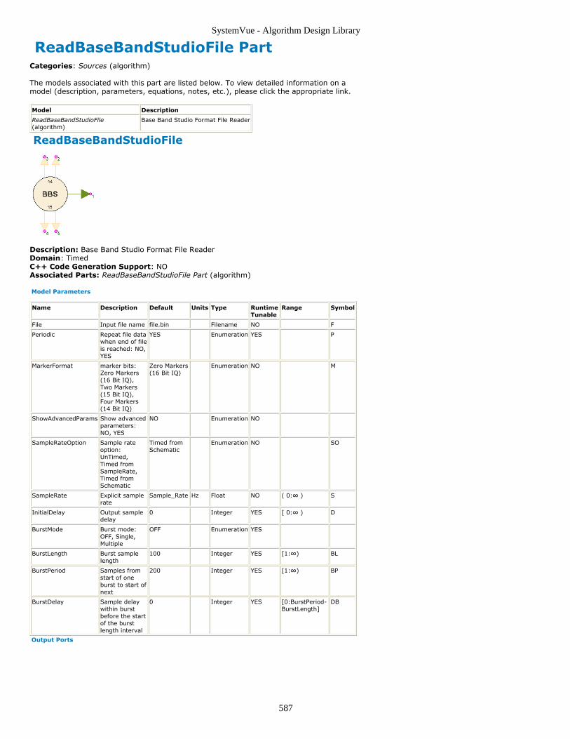
SystemVue - Algorithm Design Library
587
ReadBaseBandStudioFile PartCategories: Sources (algorithm)
The models associated with this part are listed below. To view detailed information on amodel (description, parameters, equations, notes, etc.), please click the appropriate link.
Model Description
ReadBaseBandStudioFile(algorithm)
Base Band Studio Format File Reader
ReadBaseBandStudioFile
Description: Base Band Studio Format File ReaderDomain: TimedC++ Code Generation Support: NOAssociated Parts: ReadBaseBandStudioFile Part (algorithm)
Model Parameters
Name Description Default Units Type RuntimeTunable
Range Symbol
File Input file name file.bin Filename NO F
Periodic Repeat file datawhen end of fileis reached: NO,YES
YES Enumeration YES P
MarkerFormat marker bits:Zero Markers(16 Bit IQ),Two Markers(15 Bit IQ),Four Markers(14 Bit IQ)
Zero Markers(16 Bit IQ)
Enumeration NO M
ShowAdvancedParams Show advancedparameters:NO, YES
NO Enumeration NO
SampleRateOption Sample rateoption:UnTimed,Timed fromSampleRate,Timed fromSchematic
Timed fromSchematic
Enumeration NO SO
SampleRate Explicit samplerate
Sample_Rate Hz Float NO ( 0:∞ ) S
InitialDelay Output sampledelay
0 Integer YES [ 0:∞ ) D
BurstMode Burst mode:OFF, Single,Multiple
OFF Enumeration YES
BurstLength Burst samplelength
100 Integer YES [1:∞) BL
BurstPeriod Samples fromstart of oneburst to start ofnext
200 Integer YES [1:∞) BP
BurstDelay Sample delaywithin burstbefore the startof the burstlength interval
0 Integer YES [0:BurstPeriod-BurstLength]
DB
Output Ports

SystemVue - Algorithm Design Library
588
Port Name Description Signal Type Optional
1 IQ IQ data complex NO
2 Marker14R Real Bit 14 Marker int YES
3 Marker14I Imag Bit 14 Marker int YES
4 Marker15R Real Bit 15 Marker int YES
5 Marker15I Imag Bit 15 Marker int YES
Notes/Equations
This model reads complex IQ data and, optionally, markers in the Base Band Studio1.format from a file named by the File parameter.Each Base Band Studio sample consists of a pair of 16 bit signed integers. The first2.integer hold the real parts while the second integer hold the imaginary parts.The MarkerFormat parameter specify how IQ data are encoded and how many3.markers are output. IQ data may have 14, 15 or 16 bit quantizations. With 14 bitquantization, there are four marker values, i.e. Marker14I, Marker14R, Marker15Rand Marker15I. With 15 bit quantization, there are two marker values, Marker15Rand Marker15I. With 16 bit quantization, there are no marker values.IQ is represented as a complex value with the I value in the imaginary part and the Q4.value in the real part. Both I and Q are normalized such that the absolute value ofeither never exceed unity. However, the IQ can be rescaled with a value that is readfrom a normalization file. The file name is formed from the Base Band Studio filename appended with ".Normalization.txt". This file can be editted. If such file is notavailable in the same folder as File, there is no scaling.Marker15R is taken from the least significant bit (LSB) of the first 16 bit integer.5.Marker15I is taken from the LSB of the second 16 bit integer. Similarly, Marker14Rand Marker14I are formed from the next higher LSB. These markers output zero orone. Zeros are output for a no marker value.The Base Band Studio format has implementation in ADS and is used in Agilent6.instrumentation. For more information, see CM BB StudioStreamRead .For other parameter descriptions, see File Sources (algorithm).7.Fill values are complex zeroes for IQ and integer zeros for the markers.8.Quiescent values are complex zeroes for IQ and integer zeros for the markers.9.
Important Links
Learn more about Baseband Studio from Agilent Technologies1.Also see the following related models:2.ReadFile (algorithm)ReadN5106AFile (algorithm)ReadN6030File (algorithm)ReadSignalStudioFile (algorithm)WriteBaseBandStudioFile (algorithm)WriteBaseBandStudioFileNormalize (algorithm)

SystemVue - Algorithm Design Library
589
ReadFile PartCategories: Sources (algorithm)
The models associated with this part are listed below. To view detailed information on amodel (description, parameters, equations, notes, etc.), please click the appropriate link.
Model Description
ReadFile (algorithm) Waveform Output from File
ReadN5106AFile (algorithm) N5106A Format File Reader
ReadN6030File (algorithm) N6030 Format File Reader
ReadSignalStudioFile(algorithm)
Time domain signal generator with signalstudio encrypted file baseddata
ReadFile (Waveform Output from File)
Description: Waveform Output from FileDomain: TimedC++ Code Generation Support: NOAssociated Parts: ReadFile Part (algorithm)
Model Parameters
Name Description Default Units Type RuntimeTunable
Range Symbol
File Input file name file.txt Filename NO F
Periodic Repeat file datawhen end of fileis reached: NO,YES
YES Enumeration YES P
ShowAdvancedParams Show advancedparameters:NO, YES
NO Enumeration NO
SampleRateOption Sample rateoption:UnTimed,Timed fromSampleRate,Timed fromSchematic
Timed fromSchematic
Enumeration NO SO
SampleRate Explicit samplerate
Sample_Rate Hz Float NO ( 0:∞ ) S
InitialDelay Output sampledelay
0 Integer YES [ 0:∞ ) D
BurstMode Burst mode:OFF, Single,Multiple
OFF Enumeration YES
BurstLength Burst samplelength
100 Integer YES [1:∞) BL
BurstPeriod Samples fromstart of oneburst to start ofnext
200 Integer YES [1:∞) BP
BurstDelay Sample delaywithin burstbefore the startof the burstlength interval
0 Integer YES [0:BurstPeriod-BurstLength]
DB
Output Ports
Port Name Signal Type Optional
1 output real NO
Notes/Equations
This model reads float data in ASCII text form from a file named by the File1.parameter.Float data are separated by spaces or a new line.2.For other parameter descriptions, see File Sources (algorithm).3.

SystemVue - Algorithm Design Library
590
Fill value is 0.4.Quiescent value is 0.5.
See:ReadN5106AFile (algorithm)ReadN6030File (algorithm)ReadSignalStudioFile (algorithm)ReadBaseBandStudioFile (algorithm)Sink (algorithm)
ReadN5106AFile
Description: N5106A Format File ReaderDomain: TimedC++ Code Generation Support: NOAssociated Parts: ReadFile Part (algorithm)
Model Parameters
Name Description Default Units Type RuntimeTunable
Range Symbol
File Input filename
myn5106a.bin Filename NO F
Periodic Repeat filedata when endof file isreached: NO,YES
YES Enumeration YES P
ShowAdvancedParams Showadvancedparameters:NO, YES
NO Enumeration NO
SampleRateOption Sample rateoption:UnTimed,Timed fromSampleRate,Timed fromSchematic
Timed fromSchematic
Enumeration NO SO
SampleRate Explicit samplerate
Sample_Rate Hz Float NO ( 0:∞ ) S
InitialDelay Output sampledelay
0 Integer YES [ 0:∞ ) D
BurstMode Burst mode:OFF, Single,Multiple
OFF Enumeration YES
BurstLength Burst samplelength
100 Integer YES [1:∞) BL
BurstPeriod Samples fromstart of oneburst to startof next
200 Integer YES [1:∞) BP
BurstDelay Sample delaywithin burstbefore thestart of theburst lengthinterval
0 Integer YES [0:BurstPeriod-BurstLength]
DB
Output Ports
Port Name Signal Type Optional
1 output complex NO
Notes/Equations
This model reads float data in N5106A binary format from a file named by the File1.parameter.N5106A is a binary waveform format that is targeted for use by the Agilent N5106A2.PXB MIMO Receiver Tester.For other parameter descriptions, see File Sources (algorithm).3.Fill value is 0.4.Quiescent value is 0.5.
See:ReadFile (algorithm)ReadN6030File (algorithm)

SystemVue - Algorithm Design Library
591
ReadSignalStudioFile (algorithm)ReadBaseBandStudioFile (algorithm)Sink (algorithm)
Important Links
The main purpose for this file reader is to read back the I/Q data written into a1.N5106A file by the Sink (algorithm)Learn more about the PXB/N5106A instrument from Agilent Technologies.2.To download the N5106A PXB MIMO Receiver Tester SW to run on your PC in3.simulated mode, visit the download site from Agilent Technologies.Also see the related part:4.SignalDownloader_N5106A (algorithm)
ReadN6030File
Description: N6030 Format File ReaderDomain: TimedC++ Code Generation Support: NOAssociated Parts: ReadFile Part (algorithm)
Model Parameters
Name Description Default Units Type RuntimeTunable
Range Symbol
FileI Input file name file_i.bin Filename NO FI
FileQ Input file name file_q.bin Filename NO FQ
Periodic Repeat file datawhen end of fileis reached: NO,YES
YES Enumeration YES P
ShowAdvancedParams Show advancedparameters:NO, YES
NO Enumeration NO
SampleRateOption Sample rateoption:UnTimed,Timed fromSampleRate,Timed fromSchematic
Timed fromSchematic
Enumeration NO SO
SampleRate Explicit samplerate
Sample_Rate Hz Float NO ( 0:∞ ) S
InitialDelay Output sampledelay
0 Integer YES [ 0:∞ ) D
BurstMode Burst mode:OFF, Single,Multiple
OFF Enumeration YES
BurstLength Burst samplelength
100 Integer YES [1:∞) BL
BurstPeriod Samples fromstart of oneburst to start ofnext
200 Integer YES [1:∞) BP
BurstDelay Sample delaywithin burstbefore the startof the burstlength interval
0 Integer YES [0:BurstPeriod-BurstLength]
DB
Output Ports
Port Name Description Signal Type Optional
1 output IQ data complex NO
Notes/Equations
This model reads I and Q data from the N6030 formatted files FileI and FileQ to form1.a complex IQ output.If one file is longer than the other, the shorter file will be zero padded. A warning is2.generated for this condition.IQ data is represented as a complex value with the I value in the real part and the Q3.value in the imaginary part.For other parameter descriptions, see File Sources (algorithm).4.Fill value is 0.0 + j·0.0.5.Quiescent value is 0.0 + j·0.0.6.

SystemVue - Algorithm Design Library
592
See:ReadFile (algorithm)ReadN5106AFile (algorithm)ReadSignalStudioFile (algorithm)ReadBaseBandStudioFile (algorithm)WriteN6030File (algorithm)
Important Links
Learn more about N6030 Arbitrary Waveform Generator from Agilent Technologies1.
ReadSignalStudioFile
Description: Time domain signal generator with signalstudio encrypted file based dataDomain: TimedC++ Code Generation Support: NOAssociated Parts: ReadFile Part (algorithm)
Model Parameters
Name Description Default Units Type RuntimeTunable
Range Symbol
WaveformFile Choose to either use oneof the waveform files fromSystemVue or provide awaveform file.: Built In,User Defined
Built In Enumeration NO
File input file name esg.wfm Filename NO
BuiltInFile Interal Signal Studiowaveforms: 2TONE,12TONE, CDMA2K_9CHAN,CDMA2K_PILOT,EDGE_1C_BURST,EDGE_1C_CONT,GSM_1C_BURST,GSM_1C_CONT, QAM16,QPSK, WCDMA_1DPCH,WCDMA_TM1_64DPCH_1C,WCDMA_TM1_64DPCH_4C,WCDMA_TM4,WIMAX_10MHZ_64QAM,WIMAX_10MHZ_QPSK,WLAN20MHZ54M64QAM
WLAN20MHZ54M64QAM Enumeration NO
Periodic Repeat file data when endof file is reached: NO, YES
YES Enumeration NO P
SetCarrierFrequency Set RF carrier frequency:NO, YES
NO Enumeration NO
RFCarrier RF carrier frequency (usedto overide what is specifiedin the waveform file)
1.0e9 Hz Float NO (0:∞) fc
ShowAdvancedParams Show advancedparameters: NO, YES
NO Enumeration NO
SampleRateOption Sample rate option: Timedfrom source data, Timedfrom SampleRate, Timedfrom Schematic
Timed from source data Enumeration NO SO
SampleRate Explicit sample rate Sample_Rate Hz Float NO (0:∞) S
InterpolationType Interpolation method:Sample and hold, Linear,Lagrange
Sample and hold Enumeration NO
InterpolationOrder Lagrange interpolationorder
4 Integer NO [2:∞)
InitialDelay Initial output time delay 0 s Float YES [0:∞) D
BurstMode Burst mode: OFF, Single,Multiple
OFF Enumeration YES B
BurstLength Burst time length 100e-6 s Float YES [1/SampleRate:∞) BL
BurstPeriod Time period from start ofone burst to start of next
200e-6 s Float YES [1/SampleRate:∞) BP
BurstDelay Time delay within burstbefore the start of theBurstLength interval
0 s Float YES [0:BurstPeriod-BurstLength]
DB
Output Ports

SystemVue - Algorithm Design Library
593
Port Name Signal Type Optional
1 output envelope NO
Currently without SystemVue's LTE or WiMax license, no waveform files created by Signal Studiosoftware can be read; with SystemVue's LTE or WiMax license, the corresponding waveform file (i.e.LTE or WiMax) created by Signal Studio software can be read.
With WaveformFile = Built In, there are 17 waveforms available for playback.
The ReadSignalStudioFile model can read all Agilent Signal Studio waveform format files created by otherAgilent EESof products such as ADS.
Notes/Equations
This model reads data in Signal Studio file format either from a built-in waveform file1.(WavefromFile=Built In) or from a file specified by the File parameter (WavefromFile=User Defined).The SetCarrierFrequency parameter controls the carrier frequency assigned to the2.output signal:
if set to NO, then the carrier frequency used is the one saved in the file header.if set to YES, then the carrier frequency used is the one specified in theRFCarrier parameter.
The Periodic parameter controls what happens when the simulation requires more3.data than what is stored in the file:
if set to NO, then the additional data needed has a value of 0 + j·0.if set to YES, then the data in the file is repeated.
The SampleRateOption parameter allows the user to select the sampling rate of the4.output signal:
if set to Timed from source data, then the sampling rate that is saved in the fileheader is used.if set to Timed from SampleRate, then the sampling rate specified in theSampleRate parameter is used.if set to Timed from Schematic, then the sampling rate is automaticallydetermined based on the rest of the schematic (for more details see SamplingRate Resolution (sim)).
If SampleRateOption is not set to Timed from source data, then interpolation is5.needed to get the signal values in between the actual signal samples that have beenrecorded at a different sampling rate. The InterpolationType parameter specifies theinterpolation method that will be used. There are three available option: Sample andhold, Linear, and Lagrange. When Lagrange is selected the order of interpolation isspecified in the InterpolationOrder parameter.Understand how BurstMode works (algorithm) and how it interacts with6.Periodic mode (algorithm).
In a nutshell, you can think of BurstMode = OFF equivalent to: BurstMode =1.Single, BurstLength = BurstPeriod = "Infinity", and BurstDelay = 0.When BurstMode = Multiple, each and every burst should have identical2.waveform signals. The gap between BurstPeriod and BurstLength is paddedwith 0's.Within the duration of BurstLength, if BurstLength is longer than the duration of3.the waveform provided by the Signal Studio waveform file, the following willhappen:
If Periodic = NO, then once all the samples contained in the Signal Studio1.waveform file have been read out, 0's are padded for either direct output(when SampleRateOption = Timed from source data) or for interpolation(when SampleRateOption = Timed from SampleRate or Timed fromSchematic).If Periodic = YES, then the samples contained in the Signal Studio2.waveform file will be repeatly read out for either direct output (whenSampleRateOption = Timed from source data) or for interpolation (whenSampleRateOption = Timed from SampleRate or Timed fromSchematic)
See:ReadFile (algorithm)ReadN5106AFile (algorithm)ReadN6030File (algorithm)ReadBaseBandStudioFile (algorithm)Sink (algorithm)
Important Links
Learn more about Signal Studio SW from Agilent Technologies.1.Also see the Sink (algorithm) part on how to write modulated RF simulation data into2.a Signal Studio file.
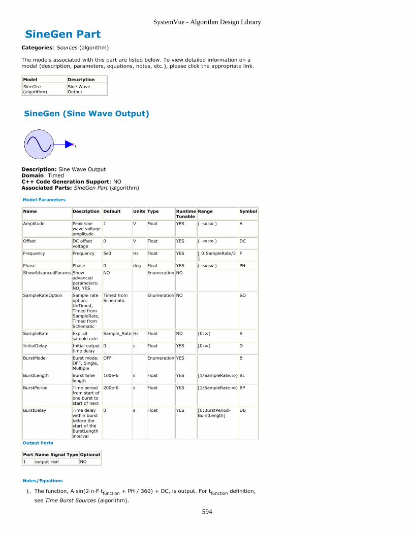
SystemVue - Algorithm Design Library
594
SineGen PartCategories: Sources (algorithm)
The models associated with this part are listed below. To view detailed information on amodel (description, parameters, equations, notes, etc.), please click the appropriate link.
Model Description
SineGen(algorithm)
Sine WaveOutput
SineGen (Sine Wave Output)
Description: Sine Wave OutputDomain: TimedC++ Code Generation Support: NOAssociated Parts: SineGen Part (algorithm)
Model Parameters
Name Description Default Units Type RuntimeTunable
Range Symbol
Amplitude Peak sinewave voltageamplitude
1 V Float YES ( -∞:∞ ) A
Offset DC offsetvoltage
0 V Float YES ( -∞:∞ ) DC
Frequency Frequency 5e3 Hz Float YES [ 0:SampleRate/2]
F
Phase Phase 0 deg Float YES ( -∞:∞ ) PH
ShowAdvancedParams Showadvancedparameters:NO, YES
NO Enumeration NO
SampleRateOption Sample rateoption:UnTimed,Timed fromSampleRate,Timed fromSchematic
Timed fromSchematic
Enumeration NO SO
SampleRate Explicitsample rate
Sample_Rate Hz Float NO (0:∞) S
InitialDelay Initial outputtime delay
0 s Float YES [0:∞) D
BurstMode Burst mode:OFF, Single,Multiple
OFF Enumeration YES B
BurstLength Burst timelength
100e-6 s Float YES [1/SampleRate:∞) BL
BurstPeriod Time periodfrom start ofone burst tostart of next
200e-6 s Float YES [1/SampleRate:∞) BP
BurstDelay Time delaywithin burstbefore thestart of theBurstLengthinterval
0 s Float YES [0:BurstPeriod-BurstLength]
DB
Output Ports
Port Name Signal Type Optional
1 output real NO
Notes/Equations
The function, A·sin(2·π·F·tfunction + PH / 360) + DC, is output. For tfunction definition,1.
see Time Burst Sources (algorithm).

SystemVue - Algorithm Design Library
595
For other parameter descriptions, see Time Burst Sources (algorithm).2.Fill value is 0.3.Quiescent value is DC.4.
See:ComplexExpGen (algorithm)SineSweepGen (algorithm)Oscillator (algorithm)

SystemVue - Algorithm Design Library
596
SineSweepGen PartCategories: Sources (algorithm)
The models associated with this part are listed below. To view detailed information on amodel (description, parameters, equations, notes, etc.), please click the appropriate link.
Model Description
SineSweepGen(algorithm)
Sine Wave Generator with Frequency Sweep
SineSweepGen (Sine Wave Generator with FrequencySweep)
Description: Sine Wave Generator with Frequency SweepDomain: TimedC++ Code Generation Support: NOAssociated Parts: SineSweepGen Part (algorithm)
Model Parameters
Name Description Default Units Type RuntimeTunable
Range Symbol
Amplitude Peak sinewavevoltageamplitude
1 V Float YES (-∞:∞) A
Offset DC offsetvoltage
0 V Float YES (-∞:∞) DC
FSweepType Frequencysweep type:linear, log
linear Enumeration YES FT
StartFreq Startfrequency
1e3 Hz Float YES (0:SampleRate/4] F1
StopFreq Stopfrequency
10e3 Hz Float YES (0:SampleRate/4] F2
Phase Phase 0 deg Float YES (-∞:∞) PH
SweepPeriod Time periodto completea sweep
Stop_Time +Time_Spacing
s Float YES [1/SampleRate:∞) SP
ShowAdvancedParams Showadvancedparameters:NO, YES
NO Enumeration NO
SampleRateOption Sample rateoption:UnTimed,Timed fromSampleRate,Timed fromSchematic
Timed fromSchematic
Enumeration NO SO
SampleRate Explicitsample rate
Sample_Rate Hz Float NO (0:∞) S
InitialDelay Initialoutput timedelay
0 s Float YES [0:∞) D
Output Ports
Port Name Signal Type Optional
1 output real NO
2 frequency real NO
Notes/Equations
Let Fi(tsweep) be the instantaneous sweep frequency defined in Time Swept Sources1.
(algorithm) and
The SineSweepGen model outputs a sinusoidal waveform of the form A·sin(2π·F(t2.sweep)·tsweep + PH / 360) + DC.
Fi(tsweep) is output at the frequency port in Hertz.3.
For other parameter descriptions, see Time Swept Sources (algorithm).4.

SystemVue - Algorithm Design Library
597
Fill value is 0.5.
See:ComplexExpGen (algorithm)SineGen (algorithm)ChirpGen (algorithm)RampSweepGen (algorithm)SquareSweepGen (algorithm)

SystemVue - Algorithm Design Library
598
SquareGen PartCategories: Sources (algorithm)
The models associated with this part are listed below. To view detailed information on amodel (description, parameters, equations, notes, etc.), please click the appropriate link.
Model Description
SquareGen(algorithm)
Square Wave Generator
SquareGen (Square Wave Generator)
Description: Square Wave GeneratorDomain: TimedC++ Code Generation Support: NOAssociated Parts: SquareGen Part (algorithm)
Model Parameters
Name Description Default Units Type RuntimeTunable
Range Symbol
LoLevel Low voltagelevel
0 V Float YES (-∞:∞) VL
HiLevel High voltagelevel
1 V Float YES (LoLevel:∞) VH
Frequency Waveformfrequency
5e3 Hz Float YES [0:SampleRate/4] F
Phase Phase 0 deg Float YES (-∞:∞) PH
DutyCycle Duty cycle inpercent
50 Float YES [100*Frequency/SampleRate:100*(1-Frequency/SampleRate)]
DC
Polarity Signalpolarity:normal,inverted
normal Enumeration YES P
ShowAdvancedParams Showadvancedparameters:NO, YES
NO Enumeration NO
SampleRateOption Sample rateoption:UnTimed,Timed fromSampleRate,Timed fromSchematic
Timed fromSchematic
Enumeration NO SO
SampleRate Explicitsample rate
Sample_Rate Hz Float NO (0:∞) S
InitialDelay Initialoutput timedelay
0 s Float YES [0:∞) D
BurstMode Burst mode:OFF, Single,Multiple
OFF Enumeration YES B
BurstLength Burst timelength
100e-6 s Float YES [1/SampleRate:∞) BL
BurstPeriod Time periodfrom start ofone burst tostart of next
200e-6 s Float YES [1/SampleRate:∞) BP
BurstDelay Time delaywithin burstbefore thestart of theBurstLengthinterval
0 s Float YES [0:BurstPeriod-BurstLength] DB
Output Ports
Port Name Signal Type Optional
1 output real NO
Notes/Equations
A square wave W(t) is defined on the t from [0, 1 / F ).1.Let tedge be the terminating edge of the square wave at DC / 100 / F.2.

SystemVue - Algorithm Design Library
599
The output W(t) for normal Polarity is:3.VH, for 0 ≤ t < tedge
VL, for tedge ≤ t < 1 / F
For inverted Polarity, the square wave begins at VL and goes to VH.4.For simulation time tfunction, t is (tfunction + PH' / 360 / F) modulo (1 / F), where PH'5.
is ((PH modulo 360) + 360) modulo 360.If zero PH, t is tfunction modulo (1 / F). For tfunction definition, see Time Burst Sources
(algorithm).For other parameter descriptions, see Time Burst Sources (algorithm).6.Fill value is 0.7.The quiescent value is:8.
VL, if Polarity (P) is normalVH, otherwise
See:SquareSweepGen (algorithm)Impulse (algorithm)PulseGen (algorithm)

SystemVue - Algorithm Design Library
600
SquareSweepGen PartCategories: Sources (algorithm)
The models associated with this part are listed below. To view detailed information on amodel (description, parameters, equations, notes, etc.), please click the appropriate link.
Model Description
SquareSweepGen(algorithm)
Square Sweep WaveGenerator
SquareSweepGen (Square Sweep Wave Generator)
Description: Square Sweep Wave GeneratorDomain: TimedC++ Code Generation Support: NOAssociated Parts: SquareSweepGen Part (algorithm)
Model Parameters
Name Description Default Units Type RuntimeTunable
Range Symbol
LoLevel Low voltagelevel
0 V Float YES (-∞:∞) VL
HiLevel High voltagelevel
1 V Float YES (LoLevel:∞) VH
FSweepType Frequencysweep type:linear, log
linear Enumeration YES FT
StartFreq Startfrequency
1e3 Hz Float YES (0:SampleRate/4] F1
StopFreq Stopfrequency
10e3 Hz Float YES (0:SampleRate/4] F2
Phase Phase 0 deg Float YES (-∞:∞) PH
SweepPeriod Time periodto completea sweep
Stop_Time +Time_Spacing
s Float YES [1/SampleRate:∞) SP
DutyCycle Duty cycle inpercent
50 Float YES [100*max(StartFreq,StopFreq)/SampleRate:100*(1-max(StartFreq,StopFreq)/SampleRate)]
DC
Polarity Signalpolarity:normal,inverted
normal Enumeration YES P
ShowAdvancedParams Showadvancedparameters:NO, YES
NO Enumeration NO
SampleRateOption Sample rateoption:UnTimed,Timed fromSampleRate,Timed fromSchematic
Timed fromSchematic
Enumeration NO SO
SampleRate Explicitsample rate
Sample_Rate Hz Float NO (0:∞) S
InitialDelay Initialoutput timedelay
0 s Float YES [0:∞) D
Output Ports
Port Name Signal Type Optional
1 output real NO
2 frequency real NO
Notes/Equations
Let Fi(tsweep) be the instantaneous sweep frequency defined in Time Swept Sources1.
(algorithm) and
A square wave function W(t') is defined on t' from [0, 1 / F(tsweep)).2.
Let tedge be DC / 100 / F(tsweep) be the terminating edge of the square wave.3.

SystemVue - Algorithm Design Library
601
Let t' be (tsweep + (PH' / 360 / F(tsweep))) modulo (1 / F(tsweep)), where PH' = ((PH4.
modulo 360) + 360) modulo 360.If PH is zero, t' is tsweep modulo ( 1 / F(tsweep)).
For normal Polarity, the output W(t') is:5.VH, if 0 ≤ t' < tedge
VL, if tedge ≤ t' < 1 / F(tsweep)
For inverted Polarity, the output W(t') is:6.VL, for 0 ≤ t' < tedge
VH, for tedge ≤ t' < 1 / F(tsweep)
Fi(tsweep) is output at the frequency port in Hertz.7.
For other parameter descriptions, see Time Swept Sources (algorithm).8.Fill value is 0.9.
See:Impulse (algorithm)PulseGen (algorithm)SquareGen (algorithm)RampSweepGen (algorithm)SineSweepGen (algorithm)

SystemVue - Algorithm Design Library
602
WalshCode PartCategories: Sources (algorithm)
The models associated with this part are listed below. To view detailed information on amodel (description, parameters, equations, notes, etc.), please click the appropriate link.
Model Description
WalshCode(algorithm)
Walsh CodeGenerator
WalshCode (Walsh Code Generator)
Description: Walsh Code GeneratorDomain: TimedC++ Code Generation Support: NOAssociated Parts: WalshCode Part (algorithm)
Model Parameters
Name Description Default Units Type RuntimeTunable
Range Symbol
WalshCodeType Walsh code type:Walsh, Hadamard,OVSF_3GPP
Walsh Enumeration YES T
Length Code length (powerof 2)
8 Integer YES [1:8192]†
L
Index Code index 0 Integer YES [0:Length- 1]
I
ShowAdvancedParams Show advancedparameters: NO,YES
NO Enumeration NO
SampleRateOption Sample rate option:UnTimed, Timedfrom SampleRate,Timed fromSchematic
Timed fromSchematic
Enumeration NO SO
SampleRate Explicit sample rate Sample_Rate Hz Float NO ( 0:∞ ) S
InitialDelay Output sampledelay
0 Integer YES [ 0:∞ ) D
Output Ports
Port Name Signal Type Optional
1 output int NO
Notes/Equations
One of three Walsh spreading codes are output.1.For Length (L), spreading codes specified with different Index (I) values are2.orthogonal.After L bits (chips), the code is reused.3.The Index parameter is N in the Walsh description or selects a matrix row in the4.Hadamard or OVSF_3GPP description.The output (chip) has index K in the Walsh description or is the K-th element of the5.matrix row in the Hadamard or OVSF_3GPP description.For Walsh, the walsh codes are defined as:6.
whereN is the index of the walsh code, [0, Length-1]N = nJ-1 nJ-2 ...n1 n0
K is the index of the chip in a walsh code, [0, Length-1]K = kJ-1 kJ-2 ...k1 k0
J = log2(Length)
r0 (n) = nJ-1
r1 (n) = nJ-1 +nJ-2
r2 (n) = nJ-2 +nJ-3
.

SystemVue - Algorithm Design Library
603
.
.rJ-1 (n) = n1 +n0
For Hadamard, the walsh codes are defined as:7.
.
.
.
For OVSF_3GPP, the walsh codes are defined as:8.
For other parameter descriptions, see Untimed Sources (algorithm).9.Fill value is 0.10.
See:RandomBits (algorithm)PRBS (algorithm)DataPattern (algorithm)
References
3GPP Technical Specification 25.213 V3.0.0 "Spreading and modulation (FDD)",1.October 1999

SystemVue - Algorithm Design Library
604
WaveForm PartCategories: Sources (algorithm)
The models associated with this part are listed below. To view detailed information on amodel (description, parameters, equations, notes, etc.), please click the appropriate link.
Model Description
WaveForm(algorithm)
Arbitrary Waveform
WaveForm (Arbitrary Waveform)
Description: Arbitrary WaveformDomain: TimedC++ Code Generation Support: NOAssociated Parts: WaveForm Part (algorithm)
Model Parameters
Name Description Default Units Type RuntimeTunable
Range Symbol
ExplicitValues Waveformvalues
[1; 1; 1; 0;0; 0]
V None NO V
Offset DC offsetvoltage
0 V None YES DC
Periodic Periodic signal:NO, YES
YES Enumeration YES P
ShowAdvancedParams Show advancedparameters:NO, YES
NO Enumeration NO
SampleRateOption Sample rateoption:UnTimed,Timed fromSampleRate,Timed fromSchematic
Timed fromSchematic
Enumeration NO SO
SampleRate Explicit samplerate
Sample_Rate Hz Float NO ( 0:∞ ) S
InitialDelay Output sampledelay
0 Integer YES [ 0:∞ ) D
BurstMode Burst mode:OFF, Single,Multiple
OFF Enumeration YES
BurstLength Burst samplelength
100 Integer YES [1:∞) BL
BurstPeriod Samples fromstart of oneburst to start ofnext
200 Integer YES [1:∞) BP
BurstDelay Sample delaywithin burstbefore the startof the burstlength interval
0 Integer YES [0:BurstPeriod-BurstLength]
DB
Output Ports
Port Name Signal Type Optional
1 output anytype NO
Notes/Equations
A waveform specified by ExplicitValues biased by DC is output. For discussion on the1.variant type, see Variant (sim).ExplicitValues is best defined with Equations. Equations can be localized to a2.schematic by creating an Equations tab in the design for the schematic.
Create a waveform of scalars by defining a variable that is a column vector, e.g.the statement, u = [0; 1; 2; 3; 4], creates a [5 x 1] matrix and defines a rampof 5 samples. Note that statement, v = [1 2 3 4 5], creates a row vector which
SystemVue - Algorithm Design Library
605
is a [1 x 5] matrix and defines a waveform that is row vector of 1 sample.Create a waveform of vectors by defining a variable that is a matrix, e.g. thestatement, u =[0 0; 1 2; 2 4; 3 6; 4 8] creates a [5 x 2] matrix and defines avector of 2 ramp waveforms of 5 samples long.Create a waveform of matrices by defining a variable with the first matrix valueand appending additional matrices with an additional right index. When finished,use the permute function to rotate the additional right index to the row indexposition. For example, the following steps creates a [5 x 2 x 2] matrix anddefines a matrix of 4 ramp waveforms of 5 samples long.
Define u as a [2 x 2] zero matrix with the statement, x = zeros(2, 2).1.Add the next 4 samples to u with the compound statement, u(:,:,2) = [1 2;2.3 4]; u(:,:,2) = [2 4; 6 8]; ... ; u(:,:,5) = [4 8; 12 16].Permute the indices of u with the statement, u = permute(u, [3 1 2]).3.
Note that waveforms of matrices with dimensionality greater than 2 can beconstructed using the previous technique.
s function = 0 always refer to first waveform value, and so on. For s function definition,3.
see Untimed Burst Sources (algorithm).If the Periodic parameter is YES, the waveform may be repeated, otherwise the4.waveform is followed by DC.For other parameter descriptions, see Untimed Burst Sources (algorithm).5.Fill value is 0.6.Quiescent value is the previous output.7.
See:ReadFile (algorithm)Window (algorithm)

SystemVue - Algorithm Design Library
606
Window PartCategories: Sources (algorithm)
The models associated with this part are listed below. To view detailed information on amodel (description, parameters, equations, notes, etc.), please click the appropriate link.
Model Description
Window(algorithm)
Window Generator
Window (Window Generator)
Description: Window GeneratorDomain: TimedC++ Code Generation Support: NOAssociated Parts: Window Part (algorithm)
Model Parameters
Name Description Default Units Type RuntimeTunable
Range Symbol
WindowType Window type:RECTANGLE,BARTLETT, HANNING,HAMMING, BLACKMAN,STEEPBLACKMAN,KAISER
HANNING Enumeration YES T
Length Window sample length 256 Integer YES [4:∞) L
ZeroPad Number of zero valuesappended to length
0 Integer YES [0:∞) Z
KaiserParameter Beta parameter 0 Float YES Beta
ShowAdvancedParams Show advancedparameters: NO, YES
NO Enumeration NO
SampleRateOption Sample rate option:UnTimed, Timed fromSampleRate, Timedfrom Schematic
Timed fromSchematic
Enumeration NO SO
SampleRate Explicit sample rate Sample_Rate Hz Float NO ( 0:∞)
S
InitialDelay Output sample delay 0 Integer YES [ 0:∞)
D
Output Ports
Port Name Signal Type Optional
1 output real NO
Notes/Equations
A periodic waveform consist of Length (L) samples of a window as selected by1.WindowType (T) followed by ZeroPad (Z) zero samples.The window is centered around its maximum in L samples.2.The KaiserParameter (Beta) value controls the stopband attenuation of the Kaiser3.window. A larger absolute value gives greater stopband attenuation.For other parameter descriptions, see Untimed Sources (algorithm).4.Fill value is 0.5.
See:ReadFile (algorithm)WaveForm (algorithm)
References
Leland Jackson, Digital Filters and Signal Processing, 2nd ed., Kluwer Academic1.Publishers, ISBN 0-89838-276-9, 1989.


![Fundamentals of Algorithm Analysis Algorithm : Design & Analysis [Tutorial - 1]](https://img.dokumen.tips/doc/110x75/5a4d1b527f8b9ab0599a8161/fundamentals-of-algorithm-analysis-algorithm-design-analysis-tutorial.jpg)
