Algorithm Design and Analysis - School Drillers

COURSE MANUAL

Algorithm Design and

Analysis CSC 236

University of Ibadan Distance Learning Centre

Open and Distance Learning Course Series Development

Copyright © 2016 by Distance Learning Centre, University of Ibadan, Ibadan.

All rights reserved. No part of this publication may be reproduced, stored in a retrieval

system, or transmitted in any form or by any means, electronic, mechanical, photocopying,

recording or otherwise, without the prior permission of the copyright owner.

ISBN: 978-021-616-2

General Editor: Prof. Bayo Okunade

University of Ibadan Distance Learning Centre

University of Ibadan,

Nigeria

Telex: 31128NG

Tel: +234 (80775935727)

E-mail: [email protected]

Website: www.dlc.ui.edu.ng

Vice-Chancellor’s Message

The Distance Learning Centre is building on a solid tradition of over two decades of service

in the provision of External Studies Programme and now Distance Learning Education in

Nigeria and beyond. The Distance Learning mode to which we are committed is providing

access to many deserving Nigerians in having access to higher education especially those who

by the nature of their engagement do not have the luxury of full time education. Recently, it is

contributing in no small measure to providing places for teeming Nigerian youths who for one

reason or the other could not get admission into the conventional universities.

These course materials have been written by writers specially trained in ODL course delivery.

The writers have made great efforts to provide up to date information, knowledge and skills in

the different disciplines and ensure that the materials are user-friendly.

In addition to provision of course materials in print and e-format, a lot of Information

Technology input has also gone into the deployment of course materials. Most of them can be

downloaded from the DLC website and are available in audio format which you can also

download into your mobile phones, IPod, MP3 among other devices to allow you listen to the

audio study sessions. Some of the study session materials have been scripted and are being

broadcast on the university’s Diamond Radio FM 101.1, while others have been delivered and

captured in audio-visual format in a classroom environment for use by our students. Detailed

information on availability and access is available on the website. We will continue in our

efforts to provide and review course materials for our courses.

However, for you to take advantage of these formats, you will need to improve on your I.T.

skills and develop requisite distance learning Culture. It is well known that, for efficient and

effective provision of Distance learning education, availability of appropriate and relevant

course materials is a sine qua non. So also, is the availability of multiple plat form for the

convenience of our students. It is in fulfilment of this, that series of course materials are being

written to enable our students study at their own pace and convenience.

It is our hope that you will put these course materials to the best use.

Prof. Abel Idowu Olayinka

Vice-Chancellor

Foreword

As part of its vision of providing education for “Liberty and Development” for Nigerians

and the International Community, the University of Ibadan, Distance Learning Centre has

recently embarked on a vigorous repositioning agenda which aimed at embracing a holistic

and all encompassing approach to the delivery of its Open Distance Learning (ODL)

programmes. Thus we are committed to global best practices in distance learning provision.

Apart from providing an efficient administrative and academic support for our students, we

are committed to providing educational resource materials for the use of our students. We are

convinced that, without an up-to-date, learner-friendly and distance learning compliant course

materials, there cannot be any basis to lay claim to being a provider of distance learning

education. Indeed, availability of appropriate course materials in multiple formats is the hub

of any distance learning provision worldwide.

In view of the above, we are vigorously pursuing as a matter of priority, the provision of

credible, learner-friendly and interactive course materials for all our courses. We

commissioned the authoring of, and review of course materials to teams of experts and their

outputs were subjected to rigorous peer review to ensure standard. The approach not only

emphasizes cognitive knowledge, but also skills and humane values which are at the core of

education, even in an ICT age.

The development of the materials which is on-going also had input from experienced editors

and illustrators who have ensured that they are accurate, current and learner-friendly. They are

specially written with distance learners in mind. This is very important because, distance

learning involves non-residential students who can often feel isolated from the community of

learners.

It is important to note that, for a distance learner to excel there is the need to source and read

relevant materials apart from this course material. Therefore, adequate supplementary reading

materials as well as other information sources are suggested in the course materials.

Apart from the responsibility for you to read this course material with others, you are also

advised to seek assistance from your course facilitators especially academic advisors during

your study even before the interactive session which is by design for revision. Your academic

advisors will assist you using convenient technology including Google Hang Out, You Tube,

Talk Fusion, etc. but you have to take advantage of these. It is also going to be of immense

advantage if you complete assignments as at when due so as to have necessary feedbacks as a

guide.

The implication of the above is that, a distance learner has a responsibility to develop

requisite distance learning culture which includes diligent and disciplined self-study, seeking

available administrative and academic support and acquisition of basic information

technology skills. This is why you are encouraged to develop your computer skills by availing

yourself the opportunity of training that the Centre’s provide and put these into use.

In conclusion, it is envisaged that the course materials would also be useful for the regular

students of tertiary institutions in Nigeria who are faced with a dearth of high quality

textbooks. We are therefore, delighted to present these titles to both our distance learning

students and the university’s regular students. We are confident that the materials will be an

invaluable resource to all.

We would like to thank all our authors, reviewers and production staff for the high quality of

work.

Best wishes.

Professor Bayo Okunade

Director

Course Development Team

Content Authoring Solomon Olalekan Akinola

Content Editor

Production Editor

Learning Design/Assessment Authoring

Managing Editor

General Editor

Prof. Remi Raji-Oyelade

Ogundele Olumuyiwa Caleb

Folajimi Olambo Fakoya

Ogunmefun Oladele Abiodun

Prof. Bayo Okunade

Table of Contents

About this course manual 1

How this course manual is structured .................................................................................................................... 1

Course Overview 3

Welcome to Algorithm Design and Analysis CIS213 ........................................................................................ 3

Getting around this course manual 4

Margin icons ....................................................................................................................................................................... 4

Study Session 1 5

Meaning, Importance and Types of Algorithms .................................................................................................. 5 Introduction .......................................................................................................................................................... 5 Terminology .......................................................................................................................................................... 5 1.1 What is an Algorithm? ............................................................................................................................... 6

1.1.1 Correct Algorithms .................................................................................................................... 6 1.1.2 Algorithm’s Performance ........................................................................................................ 6

1.2 How Do Algorithms Work?...................................................................................................................... 7 1.3 Classifications / Types of Algorithms ................................................................................................. 8

1.3.1 Simple Recursive Algorithms ................................................................................................ 8 1.3.2 Backtracking Algorithms ......................................................................................................... 9 1.3.3 Divide and Conquer ................................................................................................................... 9 1.3.4 Dynamic programming algorithms .................................................................................. 10 1.3.5 Greedy algorithms ................................................................................................................... 10 1.3.6 Branch and bound algorithms ........................................................................................... 11 1.3.7 Brute force algorithm ............................................................................................................ 12 1.3.8 Randomized algorithms ........................................................................................................ 12

1.4 The Importance of Knowing Algorithms ........................................................................................ 14 Study Session Summary ............................................................................................................................................. 15 Assessment ...................................................................................................................................................................... 15 Bibliography .................................................................................................................................................................... 16

Study Session 2 17

Problem Solving Techniques.................................................................................................................................... 17 Introduction ....................................................................................................................................................... 17 Terminology ....................................................................................................................................................... 17 2.1 What is Recursion? .................................................................................................................................. 17

Program .................................................................................................................................................... 17 Explanation ............................................................................................................................................. 18

Example 2: Recursive Fibonacci Series ..................................................................................................... 19 2.1.2 Demerits of Recursion ........................................................................................................... 20

2.2 The Divide-and-Conquer Approach ................................................................................................. 21 2.3 Backtracking ............................................................................................................................................... 22

Table of Contents ii

Study Session Summary ............................................................................................................................................. 23 Assessment ...................................................................................................................................................................... 23 Bibliography .................................................................................................................................................................... 24

Study Session 3 25

Sorting Techniques 1 ................................................................................................................................................... 25 Introduction ....................................................................................................................................................... 25 Terminology ....................................................................................................................................................... 25 3.1 Why Sorting? .............................................................................................................................................. 25 3.2 Sorting Techniques .................................................................................................................................. 26

3.2.1 Bubble Sort ................................................................................................................................. 26 A Java - Program Implementation.................................................................................... 27

3.2.2 Selection Sort............................................................................................................................. 29 3.2.3 Insertion Sort ............................................................................................................................ 29


Study Session 4 33

Sorting Techniques 2 ................................................................................................................................................... 33 Introduction ....................................................................................................................................................... 33 Terminology ....................................................................................................................................................... 33 4.1 Quick Sort .................................................................................................................................................... 33

4.1.1 Description of Quicksort ....................................................................................................... 34 4.1.2 Partitioning the Array ............................................................................................................ 35 4.1.3 Another Version of the Partitioning Algorithm .......................................................... 37 4.1.4 Choice of the key .................................................................................................................. 37

4.2 Merge Sort ................................................................................................................................................... 40 Study Session Summary ............................................................................................................................................. 46 Assessment ...................................................................................................................................................................... 47 Bibliography .................................................................................................................................................................... 47

Study Session 5 48

Searching Techniques ................................................................................................................................................. 48 Introduction ....................................................................................................................................................... 48 Terminology ....................................................................................................................................................... 48 5.1 Linear or Sequential Search ................................................................................................................. 48 5.2 Binary Search ............................................................................................................................................. 50

Program .................................................................................................................................................... 51 Study Session Summary ............................................................................................................................................. 53 Assessment ...................................................................................................................................................................... 53 Bibliography .................................................................................................................................................................... 53

Study Session 6 54

Analysis of Algorithms ................................................................................................................................................ 54 Introduction ....................................................................................................................................................... 54 Terminology ....................................................................................................................................................... 54

6.1 Runtime Analysis ...................................................................................................................................... 54 6.2 Running Time ............................................................................................................................................. 55 6.3 Time and Space Complexity of Algorithms ................................................................................... 56

6.3.1 Basic Concepts Under Time and Space Complexity .................................................. 57 6.4 Worst-Case Analysis................................................................................................................................ 58

6.4.1 Reasons for Worst-Case Analysis ..................................................................................... 58 Study Session Summary ............................................................................................................................................. 59 Assessment ...................................................................................................................................................................... 59 Bibliography .................................................................................................................................................................... 60

Study Session 7 61

The Big ‘O’ Notation ..................................................................................................................................................... 61 Introduction ....................................................................................................................................................... 61 Terminology ....................................................................................................................................................... 61 7.1 O-Notation ................................................................................................................................................... 61

7.2.1 Overview of O-Notation Rules............................................................................................ 62 7.2.2 O-Notation Example and Why It Works......................................................................... 63

7.2 Analyzing Divide-and-Conquer Algorithms .................................................................................. 64 7.3 Computational Complexity ................................................................................................................... 64

Table 7.1 Some Situations Wherein Common Complexities Occur ........................ 65 7.5 Basic Algorithm Analysis ...................................................................................................................... 68


Study Session 8 72

Run Time Analysis of Insertion Sort ..................................................................................................................... 72 Introduction ....................................................................................................................................................... 72 8.1 Running Time of Insertion Sort .......................................................................................................... 72 8.2 Order of Growth ........................................................................................................................................ 74


Study Session 9 76

Analysing Divide and Conquer Algorithms ........................................................................................................ 76 Introduction ....................................................................................................................................................... 76 9.1 Analyzing Divide and Conquer Algorithms ................................................................................... 76 9.2 Analysis of Merge Sort Algorithm ..................................................................................................... 77 9.3 Analysis of Quicksort Algorithm ........................................................................................................ 78

9.3.1 Worst Case Partitioning ........................................................................................................ 78 9.3.2 Best-Case Partitioning ........................................................................................................... 79 9.3.3 Average Case Partitioning .................................................................................................... 79

Table of Contents iv


Study Session 10 82

Growth of Functions .................................................................................................................................................... 82 Introduction ....................................................................................................................................................... 82 Terminology ....................................................................................................................................................... 82 10.1 θ-notation ................................................................................................................................................. 82

10.1.1 Big O-notation ........................................................................................................................ 83 10.1.2 Ω- notation ............................................................................................................................... 83 10.1.3 Small o-notation .................................................................................................................... 84

10.2 Small omega -notation .................................................................................................................... 84 Study Session Summary ............................................................................................................................................. 85 Assessment ...................................................................................................................................................................... 86 Bibliography .................................................................................................................................................................... 86

Study Session 11 87

Recurrences: An Overview........................................................................................................................................ 87 Introduction ....................................................................................................................................................... 87 11.1 What is Recurrence? ............................................................................................................................. 87 11.2 Technicalities........................................................................................................................................... 88 11.3 The Substitution Method .................................................................................................................... 89 11.4 Making a Good Guess ........................................................................................................................... 90 11.5 Subtleties ................................................................................................................................................... 91 11.6 Avoiding Pitfalls ..................................................................................................................................... 92 11.7 Changing Variables ............................................................................................................................... 92

Study Session Summary ............................................................................................................................................. 93 Assessment ...................................................................................................................................................................... 93

Study Session 12 94

Recurrences: Recursion-Tree Method ................................................................................................................. 94 Introduction ....................................................................................................................................................... 94 12.1 The Recursion-tree Method .............................................................................................................. 94

Study Session Summary ............................................................................................................................................. 99 Assessment ...................................................................................................................................................................... 99 Bibliography ................................................................................................................................................................. 100

Study Session 13 101

Recurrences: The Master Method ....................................................................................................................... 101 Introduction .................................................................................................................................................... 101 13.1 The Master Method ............................................................................................................................ 101 13.2 The Master Theorem ......................................................................................................................... 102

Using the master method .................................................................................................. 102

Study Session Summary .......................................................................................................................................... 103 Assessment ................................................................................................................................................................... 104 Bibliography ................................................................................................................................................................. 104

Notes on Self Assessment Questions 104

About this course manual

1

About this course manual

Algorithm Design and Analysis CSC 236 has been produced by

University of Ibadan Distance Learning Centre. All course manuals

produced by University of Ibadan Distance Learning Centreare structured

in the same way, as outlined below.

How this course manual is

structured

The course overview The course overview gives you a general introduction to the course.

Information contained in the course overview will help you determine:

If the course is suitable for you.

What you will already need to know.

What you can expect from the course.

How much time you will need to invest to complete the course.

The overview also provides guidance on:

Study skills.

Where to get help.

Course assignments and assessments.

Margin icons.

We strongly recommend that you read the overview carefully before

starting your study.

The course content The course is broken down into Study Sessions. Each Study Session

comprises:

An introduction to the Study Session content.

Study Session outcomes.

Core content of the Study Session with a variety of learning activities.

A Study Session summary.

Assignments and/or assessments, as applicable.

Bibliography

CSC 236 Algorithm Design and Analysis

2

Your comments After completing Algorithm Design and Analysis we would appreciate it

if you would take a few moments to give us your feedback on any aspect

of this course. Your feedback might include comments on:

Course content and structure.

Course reading materials and resources.

Course assignments.

Course assessments.

Course duration.

Course support (assigned tutors, technical help, etc.)

Your constructive feedback will help us to improve and enhance this

course.

Course Overview

3

Course Overview

Welcome to Algorithm Design

and Analysis CSC 2366

CSC 236 (Algorithm Design and Analysis) is a three [3] credit unit

course dealing with the fundamentals concepts of Algorithm designing

and Analysis techniques. Several sorting and searching techniques are

explored in the course.

The study material provides adequate background information that is

relevant for students to understand the concept of algorithms’ analysis.

The course is divided into two modules. The first module introduces

students to the algorithm design using sorting and searching techniques.

The second module is on the analysis of algorithms; how to measure the

time complexities of algorithms.

The Course Contents includes abstract data types, design patterns,

algorithmic issues, Searching and sorting, complexity theory, the

application and implementation of common data structures in a specific

programming language.

This is a 3 Units, Required course.

4


Getting around this course manual

Margin icons

While working through this course manual you will notice the frequent

use of margin icons. These icons serve to “signpost” a particular piece of

text, a new task or change in activity; they have been included to help you

to find your way around this course manual.

A complete icon set is shown below. We suggest that you familiarize

yourself with the icons and their meaning before starting your study.

Activity Assessment Assignment Case study

Discussion Group Activity Help Outcomes

Note Reflection Reading Study skills

Summary Terminology Time Tip

Study Session 1 Meaning, Importance and Types of Algorithms

5

Study Session 1

Meaning, Importance and Types of

Algorithms

Introduction In this session, you will be examining the meaning, importance and

types of Algorithms. You will begin by describing correct

algorithms. Thereafter, you will discuss the algorithms

performance. This will lead to the explanation of how algorithms

work. In addition, you will highlight the different classifications

and importance of algorithms.

Learning Outcomes

Outcomes

When you have studied this session, you should be able to:

1.1 define algorithm

1.2 explain how algorithms work

1.3 classify algorithms

1.4 state the importance of algorithm

Terminology

Algorithm A process or set of rules to be followed in calculations or other problem-solving operations, especially by a computer.

Mergsort In computer science, merge sort (also commonly spelled mergesort) is an efficient, general-purpose, comparison-based sorting algorithm.

Optimization An act, process, or methodology of making something (as a design, system, or decision) as fully perfect, functional, or effective as possible

6


1.1 What is an Algorithm? Informally, an algorithm is any well-defined computational procedure

that takes some value, or set of values, as input and produces some value,

or set of values, as output. An algorithm is thus a sequence of

computational steps that transform the input into the output. We can also

view an algorithm as a tool for solving a well-specified computational

problem. The following are the requirements for an algorithm:

1. An algorithm is a finite set of instructions that, if followed,

accomplishes a particular task.

2. All algorithms must satisfy the following criteria:

3. Zero or more input values

4. One or more output values

5. Clear and unambiguous instructions

6. Atomic steps that take constant time

7. No infinite sequence of steps (help, the halting problem)

8. Feasible with specified computational device

An algorithm can be specified in English, as a computer program, or even

as a hardware design. The only requirement is that the specification must

provide a precise description of the computational procedure to be

followed.

ITQ

Question

What do algorithms require?

Feedback

All algorithms must have: input values, output values, finite set of

instructions.

1.1.1 Correct Algorithms

An algorithm is said to be correct if, for every input instance, it halts with

the correct output. We say that a correct algorithm solves the given

computational problem. An incorrect algorithm might not halt at all on

some input instances, or it might halt with an answer other than the

desired one. Contrary to what one might expect, incorrect algorithms can

sometimes be useful, if their error rate can be controlled.

1.1.2 Algorithm’s Performance

Whether we are designing an algorithm or applying one that is widely

accepted, it is important to understand how the algorithm will perform.

There are a number of ways we can look at an algorithm's performance,

but usually the aspect of most interest is how fast the algorithm will run.

In some cases, if an algorithm uses significant storage, we may be

interested in its space requirement as well. Whatever the case,

determining how an algorithm performs requires a formal and

deterministic method.


7

There are many reasons to understand the performance of an algorithm.

For example, we often have a choice of several algorithms when solving

problems. Understanding how each performs helps us differentiate

between them. Understanding the burden an algorithm places on an

application also helps us plan how to use the algorithm more effectively.

For instance, garbage collection algorithms, algorithms that collect

dynamically allocated storage to return to the heap, require considerable

time to run. Knowing this, we can be careful to run them only at

opportune moments, just as LISP and Java do, for example.

1.2 How Do Algorithms Work? Let's take a closer look at an example.

A very simple example of an algorithm would be to find the largest

number in an unsorted list of numbers. If you were given a list of five

different numbers, you would have this figured out in no time, no

computer needed. Now, how about five million different numbers?

Clearly, you are going to need a computer to do this, and a computer

needs an algorithm.

Here is what the algorithm could look like. Let's say the input consists of

a list of numbers, and this list is called L. The number L1 would be the

first number in the list, L2 the second number, etc. And we know the list

is not sorted - otherwise the answer would be really easy. So, the input to

the algorithm is a list of numbers, and the output should be the largest

number in the list.

The algorithm would look something like this:

Step 1: Let Largest = L1

This means you start by assuming that the first number is the largest

number.

Step 2: For each item in the list:

This means you will go through the list of numbers one by one.

Step 3: If the item Largest:

If you find a new largest number, move to step four. If not, go back to

step two, which means you move on to the next number in the list.

Step 4: Then Largest = the item

This replaces the old largest number with the new largest number you just

found. Once this is completed, return to step two until there are no more

numbers left in the list.

Step 5: Return Largest

This produces the desired result.

Notice that the algorithm is described as a series of logical steps in a

language that is easily understood. For a computer to actually use these

instructions, they need to be written in a language that a computer can

understand, known as a programming language.

8


ITQ

Question

In which language is an algorithm written in?

Feedback

An algorithm is written in programming language. That is the only

language the computer understands.

1.3 Classifications / Types of Algorithms There is no one “correct” classification for algorithms. However,

algorithms are classified based on certain attributes.

Algorithms that use a similar problem-solving approach can be grouped

together. This classification scheme is neither exhaustive nor disjoint.

The purpose is not to be able to classify an algorithm as one type or

another, but to highlight the various ways in which a problem can be

attacked.

A short list of categories is given below:

1. Simple recursive algorithms

2. Backtracking algorithms

3. Divide and conquer algorithms

4. Dynamic programming algorithms

5. Greedy algorithms

6. Branch and bound algorithms

7. Brute force algorithms

8. Randomized algorithms

1.3.1 Simple Recursive Algorithms

A simple recursive algorithm:

1. Solves the base cases directly

2. Recurs with a simpler sub-problem

3. Does some extra work to convert the solution to the simpler sub-

problem into a solution to the given problem

They are “simple” because several of the other algorithm types are

inherently recursive

Example recursive algorithms:

1. To count the number of elements in a list:

– If the list is empty, return zero; otherwise,

– Step past the first element, and count the remaining

elements in the list

– Add one to the result

2. To test if a value occurs in a list:

– If the list is empty, return false; otherwise,

– If the first thing in the list is the given value, return true;

otherwise


9

– Step past the first element, and test whether the value

occurs in the remainder of the list

1.3.2 Backtracking Algorithms

Backtracking algorithms are based on a depth-first recursive search

A backtracking algorithm Example:

Tests to see if a solution has been found, and if so, returns it; otherwise

For each choice that can be made at this point do

1. Make that choice

2. Recur

3. If the recursion returns a solution, return it

4. End do

5. If no choices remain, return failure

Second Example:

1. To color a map with no more than four colors:

– color(Country n)

2. If all countries have been colored (n > number of countries)

return success; otherwise

3. For each color c of four colors,

4. If country n is not adjacent to a country that has been colore

Color country n with color c

recursivly color country n+1

If successful, return success

Return failure (if loop exits)

1.3.3 Divide and Conquer

A divide and conquer algorithm consists of two parts:

1. Divide the problem into smaller subproblems of the same type,

and solve these subproblems recursively

2. Combine the solutions to the subproblems into a solution to the

original problem

Traditionally, an algorithm is only called divide and conquer if it contains

two or more recursive calls

Examples:

1. Quicksort:

– Partition the array into two parts, and quicksort each of

the parts

– No additional work is required to combine the two sorted

parts

2. Mergesort:

– Cut the array in half, and mergesort each half

– Combine the two sorted arrays into a single sorted array

by merging them

3. Binary tree lookup

Here’s how to look up something in a sorted binary tree:

10


1. Compare the key to the value in the root

2. If the two values are equal, report success

3. If the key is less, search the left subtree

4. If the key is greater, search the right subtree

This is not a divide and conquer algorithm because, although there are

two recursive calls, only one is used at each level of the recursion

1.3.4 Dynamic programming algorithms

A dynamic programming algorithm remembers past results and uses them

to find new results

Dynamic programming is generally used for:

1. optimization problems

2. Multiple solutions exist, need to find the “best” one

3. Requires “optimal substructure” and “overlapping subproblems”

4. Optimal substructure: Optimal solution contains optimal

solutions to subproblems

5. Overlapping subproblems: Solutions to subproblems can be

stored and reused in a bottom-up fashion

This differs from Divide and Conquer, where subproblems generally need

not overlap

Example: Fibonacci numbers

To find the nth Fibonacci number:

1. If n is zero or one, return one; otherwise,

2. Compute, or look up in a table, fibonacci(n-1) and fibonacci(n-2

3. Find the sum of these two numbers

4. Store the result in a table and return it

Since finding the nth Fibonacci number involves finding all smaller

Fibonacci numbers, the second recursive call has little work to do. The

table may be preserved and used again later.

ITQ

Question

Algorithms are classified based on_______

Feedback

As earlier stated in the text, algorithm are classified based on ‘certain

attributes’. For instance, algorithms that use a similar problem-solving

approach can be grouped together.

1.3.5 Greedy algorithms

An optimization problem is one in which we want to find, not just a

solution, but the best solution.

A “greedy algorithm” sometimes works well for optimization problems.

A greedy algorithm works in phases: At each phase:


11

1. We take the best we can get right now, without regard for future

consequences

2. We hope that by choosing a local optimum at each step, we will

end up at a global optimum

Example: Counting money

Suppose we want to count out a certain amount of money, using the

fewest possible bills and coins, a greedy algorithm that would do this

would be: At each step, take the largest possible bill or coin that does not

overshoot.

Example: To make N6.39, you can choose:

a N5 bill

a N1 bill, to make N 6

a 25K coin, to make N 6.25

A 10K coin, to make N 6.35

four 1K coins, to make N 6.39

For the Naira and Kobo money, the greedy algorithm always

gives the optimum solution

A failure of the greedy algorithm

In some (fictional) monetary system, “krons” come in 1 kron, 7 kron, and

10 kron coins

Using a greedy algorithm to count out 15 krons, you would get

1. A 10 kron piece

2. Five 1 kron pieces, for a total of 15 krons

3. This requires six coins

A better solution would be to use two 7 kron pieces and one 1 kron piece.

This only requires three coins. The greedy algorithm results in a solution,

but not in an optimal solution

1.3.6 Branch and bound algorithms

Branch and bound algorithms are generally used for optimization

problems. As the algorithm progresses, a tree of sub-problems is formed.

The original problem is considered the “root problem”. A method is used

to construct an upper and lower bound for a given problem. At each node,

apply the bounding methods. If the bounds match, it is deemed a feasible

solution to that particular sub-problem. If bounds do not match, partition

the problem represented by that node, and make the two sub-problems

into children nodes. Continue, using the best known feasible solution to

trim sections of the tree, until all nodes have been solved or trimmed

Example branch and bound algorithm

Travelling sales-man problem: A salesman has to visit each of n cities (at

least) once each, and wants to minimize total distance travelled.

1. Consider the root problem to be the problem of finding the

shortest route through a set of cities visiting each city once

2. Split the node into two child problems:

Shortest route visiting city A first

12


Shortest route not visiting city A first

3. Continue subdividing similarly as the tree grows

1.3.7 Brute force algorithm

A brute force algorithm simply tries all possibilities until a satisfactory

solution is found. Such an algorithm can be:

1 Optimizing: Find the best solution. This may require finding all

solutions, or if a value for the best solution is known, it may stop

when any best solution is found.

Example: Finding the best path for a travelling salesman

2 Satisfying: Stop as soon as a solution is found that is good

enough.

Example: Finding a travelling salesman path that is within 10%

of optimal

Often, brute force algorithms require exponential time. Various heuristics

and optimizations can be used. These are:

1. Heuristic: A “rule of thumb” that helps you decide which

possibilities to look at first

2. Optimization: In this case, a way to eliminate certain possibilities

without fully exploring them.

ITQ

Question

What attribute qualifies an algorithm as a divide and conquer type? List

two examples of divide and conquer algorithm?

Feedback

As earlier stated in the text, an algorithm is only called divide and

conquer if it contains two or more recursive calls. Two examples of

divide and conquer algorithm are Quicksort and Mergesort.

1.3.8 Randomized algorithms

A randomized algorithm uses a random number at least once during the

computation to make a decision.

Examples:

1 In Quicksort, using a random number to choose a pivot

2 Trying to factor a large prime by choosing random numbers as

possible divisors

Other Categories of Algorithms are:

1. Deterministic vs. Randomized: One important (and exclusive)

distinction one can make is, whether the algorithm is

deterministic or randomized. Deterministic algorithms produce

on a given input the same results following the same computation

steps. Randomized algorithms throw coins during execution.

Hence either the order of execution or the result of the algorithm

might be different for each run on the same input. There are

subclasses for randomized algorithms: Monte Carlo type


13

algorithms and Las Vegas type algorithms. A Las Vegas

algorithm will always produce the same result on a given input.

Randomization will only affect the order of the internal

executions.

In the case of Monte Carlo algorithms, the result may might

change, even be wrong. However, a Monte Carlo algorithm will

produce the correct result with a certain probability. So of course

the question arises: What are randomized algorithms good for?

The computation might change depending on coin throws. Monte

Carlo algorithms do not even have to produce the correct result.

Why would that be desirable? The answer is twofold:

i. Randomized algorithms usually have the effect of

perturbing the input. Or put it differently, the input looks

random, which makes bad cases very seldom.

ii. Randomized algorithms are often conceptually very easy to

implement. At the same time they are in run time often

superior to their deterministic counterparts. Can you think

of an obvious example?

2. Offline vs. Online: Another important (and exclusive) distinction

one can make is, whether the algorithm is offline or online.

Online algorithms are algorithms that do not know their input at

the beginning. It is given to them online, whereas normally

algorithms know their input beforehand. What seems like a minor

detail has profound effects on the design of algorithms and on

their analysis. Online algorithms are usually analyzed by using

the concept of competitiveness, that is the worst case factor they

take longer compared to the best algorithm with complete

information.

3. Exact vs approximate vs. heuristic vs. operational: Usually

algorithms have an optimization goal in mind, e.g. compute the

shortest path or the alignment or minimal edit distance. Exact

algorithms aim at computing the optimal solution given such a

goal. Often this is quite expensive in terms of run time or

memory and hence not possible for large input. In such cases one

tries other strategies. Approximation algorithms aim at

computing a solution which is for example only a certain,

guaranteed factor worse than the optimal solution, that means an

algorithm yields a c - approximation, if it can guarantee that its

solution is never worse than a factor c compared to the optimal

solution. Alternatively, heuristic algorithms try to reach the

optimal solution without giving a guarantee that they always do.

Often it is easy to construct a counter example. A good heuristics

is almost always near or at the optimal value.

Finally there are algorithms which do not aim at optimizing an objective

function. Let’s call them operational since they chain a series of

computational operations guided by expert knowledge but not in

conjunction with a specific objective function (e.g. ClustalW).

Example: Approximation algorithm

As an example think of the Travelling Salesman Problem with triangle

inequality for n cities. This is an NP-hard problem (no polynomial-time

14


algorithm is known). The following greedy, deterministic algorithm

yields a 2-approximation for the TSP with triangle inequality in time

O(n2).

1. Compute a minimum spanning tree T for the complete graph

implied by the n cities.

2. Duplicate all edges of T yielding a Eulerian graph T’ and then

find an Eulerian path in T’.

3. Convert the Eulerian cycle into a Hamiltonian cycle by taking

shortcuts.

Can you now argue why this is a 2-approximation?

ITQ

Question

What is an optimization problem? List two examples of algorithms

generally used in solving optimization problems.

Feedback

An optimization problem is one in which we want to find, not just a

solution but the best solution. Examples of algorithms used in solving

optimization problem include Dynamic programming algorithms,

Greedy algorithms, Branch and bound algorithms.

1.4 The Importance of Knowing Algorithms As a computer scientist, it is important to understand all of these types of

algorithms so that one can use them properly. If you are working on an

important piece of software, you will likely need to be able to estimate

how fast it is going to run. Such an estimate will be less accurate without

an understanding of runtime analysis. Furthermore, you need to

understand the details of the algorithms involved so that you’ll be able to

predict if there are special cases in which the software won’t work

quickly, or if it will produce unacceptable results.

Of course, there are often times when you’ll run across a problem that has

not been previously studied. In these cases, you have to come up with a

new algorithm, or apply an old algorithm in a new way. The more you

know about algorithms in this case, the better your chances are of finding

a good way to solve the problem. In many cases, a new problem can be

reduced to an old problem without too much effort, but you will need to

have a fundamental understanding of the old problem in order to do this.

As an example of this, let’s consider what a switch does on the Internet.

A switch has N cables plugged into it, and receives packets of data

coming in from the cables. The switch has to first analyze the packets,

and then send them back out on the correct cables. A switch, like a

computer, is run by a clock with discrete steps – the packets are sent out

at discrete intervals, rather than continuously. In a fast switch, we want to

send out as many packets as possible during each interval so they don’t

stack up and get dropped. The goal of the algorithm we want to develop

is to send out as many packets as possible during each interval, and also


15

to send them out so that the ones that arrived earlier get sent out earlier.

In this case it turns out that an algorithm for a problem that is known as

"stable matching" is directly applicable to our problem, though at first

glance this relationship seems unlikely. Only through pre-existing

algorithmic knowledge and understanding can such a relationship be

discovered.

Other examples of real-world problems with solutions requiring advanced

algorithms abound. Almost everything that you do with a computer relies

in some way on an algorithm that someone has worked very hard to

figure out. Even the simplest application on a modern computer would

not be possible without algorithms being utilized behind the scenes to

manage memory and load data from the hard drive.

ITQ

Question

Now I want you to think of other real life examples where algorithms are

applicable.

Feedback

Algorithm are applicable everywhere, in the use of your laptops, mobile

phones and even in many household appliances. Algorithm are essential

in the sending of mails and messages over the internet.

Study Session Summary

Summary

In this session, you examined algorithms. You began by

explaining what an algorithm is. Thereafter, you discusses correct

algorithm and algorithms performance. Moving on, you explained

how algorithms work. In addition, you noted the different

classifications of algorithms. Lastly, you discussed why the

knowledge of algorithms is important.

Assessment

Assessment

SAQ 1.1 (tests Learning Outcome 1.1)

What is an algorithm?


Explain how algorithms work

SAQ 1.3 (Learning Outcome 1.3)

How do we classify algorithms?

SAQ 1.4 (Learning Outcome 1.4)

What do you consider as the importance of knowing algorithm?

16


Bibliography

Reading

http://www.bbc.co.uk/guides/z3whpv4 retrieved January 2017

http://whatis.techtarget.com/definition/algorithm retrieved January 2017

https://www.coursera.org/learn/introduction-to-algorithms retrieved

January 2017

http://www.bbc.co.uk/guides/z3whpv4

http://whatis.techtarget.com/definition/algorithm

https://www.coursera.org/learn/introduction-to-algorithms

Study Session 2 Problem Solving Techniques

17

Study Session 2

Problem Solving Techniques

Introduction In this study session, you will be discussing the different problem solving

techniques in programming. You will begin by explaining what a

recursion is. After this, you will make attempt at comparing recursion and

iteration techniques. Likewise, you will explain the divide-and-conquer

approach. Finally, you will look at the backtracking problem solving

technique.

Learning Outcomes

Outcomes


2.1 define recursion

2.2 discuss the divide-and-conquer approach

2.3 compare recursion and iteration

2.4 define backtracking

Terminology

Fibonacci The series of numbers: 0, 1, 1, 2, 3, 5, 8, 13, 21, 34, ... The next number is found by adding up the two numbers

2.1 What is Recursion? Recursion is a powerful principle that allows something to be

defined in terms of smaller instances of itself. In computing,

recursion is supported via recursive functions. A recursive function

is a function that calls itself. Each successive call works on a more

refined set of inputs, bringing us closer and closer to the solution of

a problem. You can express most of the problems in the following

program by using recursion. We represent the function add by

using recursion.

Program

#include <stdio.h>

int add(int pk,int pm);

main( )

18


int k, i, m;

m = 2;

k = 3;

i = add(k, m);.

printf("The value of addition is %d\n",i);

int add(int pk,int pm)

if(pm = = 0)

return pk; \\ A

else

return (1 + add(pk, pm-1)); \\ B

Explanation

1. The add function is recursive as follows:

add (x, y) = 1 + add(x, y-1) y > 0

= x y = 0

for example,

add(3, 2) = 1 + add(3, 4)

add(3, 1) = 1 + add(3, 0)

add(3, 0) = 3

add(3, 1) = 1+3 = 4

add(3, 2) = 1+4 = 5

2. The recursive expression is 1+add(pk, pm-1). The

terminating condition is pm = 0 and the recursive condition

is pm > 0.

A function can call itself in a number of times. A recursive method

is one that calls itself either directly or indirectly through another

method.

In recursion, the problems being solved are similar in nature and

their solutions too are similar. When a recursive method/function is

called to solve a problem, the method could actually solve the

simplest case or base case. If the method is called with a base case,

the method returns a result. However, if the method is called with a


19

complex problem, it divides the problem into two conceptual

pieces: a piece that the method knows how to solve (the base case)

and a piece that the method does not know how to solve. The latter

piece must resemble the original problem but be a slightly simpler

or slightly smaller version of it. Because this new problem looks

like the original problem, the method calls a fresh copy of itself to

work on the small problem. This procedure is called a recursive

call or recursion step. The recursion step must include a return

statement because its result will be combined with the portion of

the problem the method knew how to solve to form a result that

will passed back to the original caller.

The recursion step executes while the original call has not finished

executing. As a matter of fact, there could be many recursion calls,

as the method divides each new subproblem into two conceptual

pieces.

Example 1: Factorial

The factorial of a number is given as n! = n x (n – 1) x (n – 2) ….. x 2.

The function below computes the factorial of n, function fac assumes that

the factorial of any numbers less or equal to 1 is zero.

// The Factorial function

long fac(int n)

if (n <= 1)

return 1;

long f = 1;

for (int i = n; i >= 2; i--)

f = f*i;

return f;

The function is implemented recursively below:

long fac (int n)

// Base case

if (n <= 1)

return 1;

//Recursive step

else

return n * fac(n – 1);

// End function fac

Example 2: Recursive Fibonacci Series

Consider the Fibonacci series: 0, 1, 1, 2, 3, 5, 8, 13, 21, ….

20


The series begins with 0 and 1 and has the property that each subsequent

Fibonacci number is the sum of the previous two Fibonacci numbers. The

ratio of successive Fibonacci numbers converges on a constant value

1.618, a number called the golden ratio or golden mean. The Fibonacci

model equation is given as:

Fibonacci(0) = 0

Fibonacci(1) = 1

Fibonacci(n) = Fibonacci(n – 1) + Fibonacci(n – 2)

long fib (int n)

// Base case

if (n == 0 || n == 1)

return n;

// Recursive step

else

return fib(n – 1) + fib(n – 2);

// End method fib

Comparing Recursion and Iteration

We can compare recursion and iteration as follows:

1. Both iteration and recursion are based on a control statement:

iteration uses a repetition control (for, while or do- while);

recursion uses a selection control (if, if – else or switch).

2. Both involve repetition: Iteration explicitly uses a repetition

statement, recursion achieves repetition through repeated

method calls.

3. Both involve a termination test: Iteration terminates when the

loop continuation condition fails. Recursion terminates when

a base case is recognized.

4. Iteration with counter-controlled repetition and recursion,

each gradually approach termination: iteration keeps

modifying a counter until the counter assumes a value that

makes the loop continuation condition fail, recursion keeps

producing simpler versions of the original problem until the

base case is reached.

5. Both can occur infinitely: an infinite loop occurs with

iteration if the loop continuation test never becomes false.

Infinite recursion occurs if the recursion step does not reduce

the problem each time in a manner that converges on the base

case.

2.1.2 Demerits of Recursion

It repeatedly invokes the mechanism, and consequently, the overhead, of

method calls. This repetition can be expensive in terms of both processor

time and memory space. Each recursive call causes another copy of the

method (actually, only the method’s variables) to be created; this set of


21

copies can consume considerable memory space. Iteration occurs within a

method, so repeated method calls and extra memory assignment are

avoided. Therefore, there is no need of choosing recursion.

ITQ

Question

What are the demerits of Recursion?

Feedback

The demerit of recursion is the increase in the overhead cost of calls in

term of processor time and memory space, as a result of its repetitive

mechanism. Each recursive call causes another copy of the method to be

created; this set of copies can consume considerable memory space.

2.2 The Divide-and-Conquer Approach Many useful algorithms are recursive in structure: to solve a given

problem, they call themselves recursively one or more times to deal

with closely related subproblems. These algorithms typically

follow a divide-and-conquer approach: they break the problem into

several subproblems that are similar to the original problem but

smaller in size, solve the subproblems recursively, and then

combine these solutions to create a solution to the original problem.

The divide-and-conquer paradigm involves three steps at each level

of the recursion:

1. Divide the problem into a number of subproblems.

2. Conquer the subproblems by solving them recursively. If

the subproblem sizes are small enough, however, just solve

the subproblems in a straightforward manner.

3. Combine the solutions to the subproblems into the solution

for the original problem.

The merge sort algorithm closely follows the divide-and-conquer

paradigm. Intuitively, it operates as follows.

1. Divide: Divide the n-element sequence to be sorted into two

subsequences of n/2 elements each.

2. Conquer: Sort the two subsequences recursively using

merge sort.

3. Combine: Merge the two sorted subsequences to produce

the sorted answer.

The recursion "bottoms out" when the sequence to be sorted has

length 1, in which case there is no work to be done, since every

sequence of length 1 is already in sorted order.

22


2.3 Backtracking Suppose you have to make a series of decisions, among various choices,

where:

1. You don’t have enough information to know what to choose

2. Each decision leads to a new set of choices

3. Some sequence of choices (possibly more than one) may be a

solution to your problem

Backtracking is a methodical way of trying out various sequences of

decisions, until you find one that “works”

Example: Solving a puzzle

1. In this puzzle, all holes but one are filled with white pegs

2. You can jump over one peg with another

3. Jumped pegs are removed

4. The object is to remove all but the last peg

5. You don’t have enough information to jump correctly

6. Each choice leads to another set of choices

7. One or more sequences of choices may (or may not) lead to a

solution

8. Many kinds of puzzle can be solved with backtracking


23

ITQ

Question

In your own words, can you illustrate what backtracking is?

Feedback

Interestingly, backtracking is like playing a chess game on your laptop

with an undo function. Lets say you are at the endgame, and you are

looking for a way to checkmate your opponent. If you try a move and it

doesn’t work, you click on undo and you have the opportunity to redo

that move, if you keep clicking “undo” till you finally checkmate your

opponent. You’ve successfully backtracked!!!


Summary

In this study session, you discussed the different problem solving

technique. You started by explaining what a recursion technique is.

Subsequently, you made attempt at comparing recursion and iteration

techniques. Likewise, you will highlight the different demerits of

recursion. Furthermore, you will explained the divide-and-conquer

approach of problem solving technique. Lastly, you will describe the

backtracking technique of problem solving.

Assessment

Assessment


What is recursion?


24


Discuss divide and conquer approach?


Define backtracking.

Bibliography

Reading

https://en.wikipedia.org/wiki/Recursion_%28computer_science%29

retrieved January 2017

http://stackoverflow.com/questions/3021/what-is-recursion-and-when-

should-i-use-it retrieved January 2017

https://interactivepython.org/runestone/static/pythonds/Introduction/Wh

atIsComputerScience.html retrieved January 2017

https://en.wikipedia.org/wiki/Recursion_%28computer_science%29

http://stackoverflow.com/questions/3021/what-is-recursion-and-when-should-i-use-it

http://stackoverflow.com/questions/3021/what-is-recursion-and-when-should-i-use-it

https://interactivepython.org/runestone/static/pythonds/Introduction/WhatIsComputerScience.html

https://interactivepython.org/runestone/static/pythonds/Introduction/WhatIsComputerScience.html

Study Session 3 Sorting Techniques 1

25

Study Session 3

Sorting Techniques 1

Introduction In this study session, you will be discussing sorting technique. You

will start by explaining why sorting technique is necessary. After

this, you will describe the bubble sort and selection sort.

Learning Outcomes

Outcomes


3.1 discuss the reasons for sorting

3.2 explain bubble sort

3.3 discuss selection sorting

Terminology

Subroutine In computer programming, a subroutine is a sequence of program instructions that perform a specific task, packaged as a unit.

3.1 Why Sorting? Many computer scientists consider sorting to be the most fundamental

problem in the study of algorithms. There are several reasons:

1. Sometimes the need to sort information is inherent in an

application. For example, in order to prepare customer

statements, banks need to sort checks by check number.

2. Algorithms often use sorting as a key subroutine. For example, a

program that renders graphical objects that are layered on top of

each other might have to sort the objects according to an "above"

relation so that it can draw these objects from bottom to top. We

shall see numerous algorithms in this text that use sorting as a

subroutine.

3. There is a wide variety of sorting algorithms, and they use a rich

set of techniques. In fact, many important techniques used

throughout algorithm design are represented in the body of

sorting algorithms that have been developed over the years. In

this way, sorting is also a problem of historical interest.

26


4. Sorting is a problem for which we can prove a nontrivial lower

bound. Our best upper bounds match the lower bound

asymptotically, and so we know that our sorting algorithms are

asymptotically optimal. Moreover, we can use the lower bound

for sorting to prove lower bounds for certain other problems.

5. Many engineering issues come to the fore when implementing

sorting algorithms. The fastest sorting program for a particular

situation may depend on many factors, such as prior knowledge

about the keys and satellite data, the memory hierarchy (caches

and virtual memory) of the host computer, and the software

environment. Many of these issues are best dealt with at the

algorithmic level, rather than by "tweaking" the code.

3.2 Sorting Techniques Some of the important sorting techniques are discussed here.

3.2.1 Bubble Sort

Bubble sort is a popular sorting algorithm. It works by repeatedly

swapping adjacent elements that are out of order.

Version 1:

BUBBLESORT(A)

1 for i ← 1 to length[A] do

2 for j ← i + 1 to length[A]

3 if A[j] < A[i]

4 then exchange A[j] ↔ A[j - 1]

Version 2:

BUBBLESORT(A)

1 for i ← 1 to length[A] do

2 for j ← length[A] downto i + 1 do

3 if A[j] < A[j - 1]

4 then exchange A[j] ↔ A[j - 1]

Bubble sorting is a simple sorting technique in which we arrange the

elements of the list by forming pairs of adjacent elements. That means we

form the pair of the ith and (i+1)th

element. If the order is ascending, we

interchange the elements of the pair if the first element of the pair is

greater than the second element. That means for every pair

(list[i],list[i+1]) for i :=1 to (n−1) if list[i] > list[i+1], we need to

interchange list[i] and list[i+1].

Carrying this out once will move the element with the highest value to the

last or nth position. Therefore, we repeat this process the next time with

the elements from the first to (n−1)th positions. This will bring the

highest value from among the remaining (n−1) values to the (n−1)th


27

position. We repeat the process with the remaining (n−2) values and so

on.

Finally, we arrange the elements in ascending order. This requires to

perform (n−1) passes. In the first pass we have (n−1) pairs, in the second

pass we have (n−2) pairs, and in the last (or (n−1)th) pass, we have only

one pair. Therefore, the number of probes or comparisons that are

required to be carried out is:

and the order of the algorithm is O(n2).

A Java - Program Implementation

import java.util.Scanner;

public class bubblesort

//Method to sort the data using bubble sort

public static void Bsort(int A[ ])

for (int i = 0; i < A.length; i++)

for (int j = (i + 1); j < A.length; j++)

if (A[i] > A[j])

int temp = A[j];

A[j] = A[i];

A[i] = temp;

//end if

next j

// next i

//Printing the sorted array

System.out.print("The final sorted list is shown below \n\n");


System.out.print(A[i] + "\t");

//Ending Method Bsort

public static void main(String[ ] args)

Scanner input = new Scanner(System.in);

System.out.println("How many data to sort?");

int n = input.nextInt();

// Declaring the array

28


int A[ ] = new int[n];

//Inserting data into the array


System.out.println("Enter data at location " + (i+1));

A[i] = input.nextInt( );

//Calling the Bsort function

bubblesort.Bsort(A);

System.out.print("\nThanks for using this program");

Sample run of the program

How many data to sort?

5

Enter data at location 1

3


1


5


4


2

The final sorted list is shown below

1 2 3 4 5

Thanks for using this program


29

3.2.2 Selection Sort

Consider sorting n numbers stored in array A by first finding the smallest

element of A and exchanging it with the element in A[1]. Then find the

second smallest element of A, and exchange it with A[2]. Continue in this

manner for the first n - 1 elements of A. This technique is known as

selection sort. The pseudocode below gives the Selection Sort Algorithm.

Select_Sort(A)

Select_Sort(A)

(1) for (i = 0; i < n-1; i++)

(2) small = i;

(3) for (j = i+1; j < n; j++)

(4) if (A[j] < A[small])

(5) small = j;

// next j

(6) temp = A[small];

(7) A[small] = A[i];

(8) A[i] = temp;

//next i

// end select_sort

Practical Work: Attempt to implement the Selection sort in any

programming language of your choice

3.2.3 Insertion Sort

Insertion sort is one of the simplest sorting algorithms. It works like the

approach we might use to systematically sort a pile of cancelled checks

by hand. We begin with a pile of unsorted checks and space for a sorted

pile, which initially contains no checks. One at a time, we remove a

check from the unsorted pile and, considering its number, insert it at the

proper position among the sorted checks.

More formally, insertion sort takes one element at a time from an

unsorted set and inserts it into a sorted one by scanning the set of sorted

elements to determine where the new element belongs.

Although at first it may seem that insertion sort would require space for

both the sorted and unsorted sets of data independently, it actually sorts in

place.

Example 1. A C Implementation of Insertion Sort

#include <stdio.h>

// The Insertion Sort function...

void insert(int A[], int n)

30


int i, j, key;

for (j = 1; j < n; j++)

key = A[j];

i = j - 1;

while ((i > -1) && (A[i] > key))

A[i + 1] = A[i];

i = i - 1;

//end while

A[i + 1] = key;

//next j

// end function insert

main( )

int i, A[10];

// Getting the original array

printf(" Sorting Program using Insertion Sorting technique \n \n");

printf("Enter only integer numeric data please\n\n");

for (i = 0; i < 10; i++)

printf("Enter data %d ", i + 1);

scanf("%d", &A[i]);

// next data

// printing the Original unsorted data

printf("\nThe original unsorted data here:\n\n");

for (i = 0; i < 10; i++)

printf("%d\t", A[i]);

// Call the insert insertion sort routine

insert(A, 10);

printf("\n ");

// printing the sorted data

printf("\n\nThe sorted data here:\n\n\n");


31

for (i = 0; i < 10; i++)

printf("%d\t", A[i]);

// end main

ITQ

Question

What is insertion sorting?

Feedback

Insertion sort is one of the simplest sorting algorithms. Insertion sort

takes one element at a time from an unsorted set and inserts it into a

sorted one by scanning the set of sorted elements to determine where the

new element belongs.


Summary

In this study session, you discussed the sorting technique. You

started by explaining why sorting technique is important. In

addition, you described the different sorting techniques.

Specifically, the techniques include bubble sort, selection sort and

insertion sort.

Assessment

Assessment


i. Define Sorting

ii. Outline the reasons for sorting


32


i. Explain Bubble sort.

ii. Define selection sorting.

Bibliography

Reading

https://www.cs.cmu.edu/~adamchik/15-

121/lectures/Sorting%20Algorithms/sorting.html retrieved January 2017

https://en.wikipedia.org/wiki/Bubble_sort retrieved January 2017

https://www.cs.cmu.edu/~adamchik/15-121/lectures/Sorting%20Algorithms/sorting.html

https://www.cs.cmu.edu/~adamchik/15-121/lectures/Sorting%20Algorithms/sorting.html

https://en.wikipedia.org/wiki/Bubble_sort


33

Study Session 4

Sorting Techniques 2

Introduction In the last study session, you discussed the sorting technique. In

this study session, you will continue with the sorting technique by

describing the quick sort. In order to do this, you will describe what

quick sorting is. You will also describe how to partition the array

and also discuss the other version of the partitioning algorithms.

Finally, you will evaluate the merge sort.

Learning Outcomes

Outcomes


4.1 define quick sort

4.2 explain merge sort

Terminology

Initialize Set to the value or put in the condition appropriate to the start of an operation.

Subsists Maintain or support oneself, especially at a minimal level.

Merge sort (also commonly spelled mergesort) is an efficient, general-purpose, comparison-based sorting algorithm

sub arrays In computer science, merge sort (also commonly spelled mergesort) is an efficient, general-purpose, comparison-based sorting algorithm

4.1 Quick Sort In the quick sort method, an array a[1],…..,a[n] is sorted by selecting

some value in the array as a key element. We then swap the first element

of the list with the key element so that the key will be in the first position.

We then determine the key's proper place in the list. The proper place for

the key is one in which all elements to the left of the key are smaller than

the key, and all elements to the right are larger.

34


To obtain the key's proper position, we traverse the list in both directions

using the indices i and j, respectively. We initialize i to that index that is

one more than the index of the key element. That is, if the list to be sorted

has the indices running from m to n, the key element is at index m, hence

we initialize i to (m+1). The index i is incremented until we get an

element at the ith position that is greater than the key value. Similarly, we

initialize j to n and go on decrementing j until we get an element with a

value less than the key's value.

We then check to see whether the values of i and j have crossed each

other. If not, we interchange the elements at the key (mth)position with

the elements at the jth position. This brings the key element to the j

th

position, and we find that the elements to its left are less than it, and the

elements to its right are greater than it. Therefore we can split the list into

two sublists. The first sublist is composed of elements from the mth

position to the (j–1)th position, and the second sublist consists of elements

from the (j+1)th position to the n

th position. We then repeat the same

procedure on each of the sublists separately.

ITQ

Question

Briefly summarize the Quick Sort Method

Feedback

The quick sort method is a sorting algorithm that sorts element in a list

into a particular order based on the position of the key element. In quick

sort method, an array a[1],…..,a[n] is sorted by selecting some value in

the array as a key element. The key element is swap with the first

element on the list so that the key element will be in the first position.

We then determine the key element's proper place in the list. The proper

place for the key is one in which all elements to the left of the key are

smaller than the key, and all elements to the right are larger.

4.1.1 Description of Quicksort

Quicksort, like merge sort, is based on the divide-and-conquer paradigm.

Here is the three-step divide-and-conquer process for sorting a typical

subarray A[p ‥ r].

Divide: Partition (rearrange) the array A[p ‥ r] into two

(possibly empty) subarrays A[p ‥ q - 1] and A[q + 1 ‥ r] such

that each element of A[p ‥ q - 1] is less than or equal to A[q],

which is, in turn, less than or equal to each element of A[q + 1 ‥

r]. Compute the index q as part of this partitioning procedure.

Conquer: Sort the two subarrays A[p ‥ q -1] and A[q +1 ‥ r]

by recursive calls to quicksort.

Combine: Since the subarrays are sorted in place, no work is

needed to combine them: the entire array A[p ‥ r] is now sorted.

The following procedure implements quicksort.


35

QUICKSORT(A, p, r)

1 if p < r

2 then q = PARTITION(A, p, r)

3 QUICKSORT(A, p, q - 1)

4 QUICKSORT(A, q + 1, r)

To sort an entire array A, the initial call is QUICKSORT(A, 1,

length[A]).

ITQ

Question

Describe the Quick Sort Method.

Feedback

The Quick sort is a divide and conquer algorithm. It divides an array into

subarray: the low elements and the high elements. For example, you

have an array A. This quick sort method partitions the array A[p ‥ r]

into two subarrays A[p ‥ q - 1] and A[q + 1 ‥ r] such that each

element of A[p ‥ q - 1] is less than or equal to A[q], which is, in turn,

less than or equal to each element of A[q + 1 ‥ r]. This method

compute the index q as part of this partitioning procedure. Then sort the

two subarrays A[p ‥ q -1] and A[q +1 ‥ r] by recursive calls to

quicksort. Lastly, since the subarrays are sorted in place, no work is

needed to combine them: the entire array A[p ‥ r] is now sorted.

4.1.2 Partitioning the Array

The key to the algorithm is the PARTITION procedure, which rearranges

the subarray A[p ‥ r] in place.

PARTITION(A, p, r)

1 x ← A[r]

2 i ← p - 1

3 for j ← p to r - 1

4 do if A[j] ≤ x

5 then i ← i + 1

6 exchange A[i] ↔ A[j]

7 exchange A[i + 1] ↔ A[r]

8 return i + 1

36


Figure 4.1 shows the operation of PARTITION on an 8-element array.

PARTITION always selects an element x = A[r] as a pivot element

around which to partition the subarray A[p ‥ r]. As the procedure runs,

the array is partitioned into four (possibly empty) regions. At the start of

each iteration of the for loop in lines 3-6, each region satisfies certain

properties, which we can state as a loop invariant:

Figure 4.1: The operation of PARTITION on a sample array.

Lightly shaded array elements are all in the first partition with values no

greater than x. Heavily shaded elements are in the second partition with

values greater than x. The un-shaded elements have not yet been put in

one of the first two partitions, and the final white element is the pivot.

(a) The initial array and variable settings. None of the elements have been

placed in either of the first two partitions.

(b) The value 2 is "swapped with itself" and put in the partition of smaller

values.

(c)-(d) The values 8 and 7 are added to the partition of larger values.

(e) The values 1 and 8 are swapped, and the smaller partition Grows.

(f) The values 3 and 8 are swapped, and the smaller partition grows.

(g)-(h) The larger partition grows to include 5 and 6 and the loop

terminates.

(i) In lines 7-8, the pivot element is swapped so that it lies between the

two partitions.

At the beginning of each iteration of the loop of lines 3-6, for any array

index k,

If p ≤ k ≤ i, then A[k] ≤ x.

If i + 1 ≤ k ≤ j - 1, then A[k] > x.

If k = r, then A[k] = x.


37

4.1.3 Another Version of the Partitioning

Algorithm

QUICKSORT(A, p, r)

1 if p < r

2 then q = PARTITION(A, p, r)

3 QUICKSORT(A, p, q - 1)

4 QUICKSORT(A, q + 1, r)

HOARE-PARTITION(A, p, r)

1 x ← A[p] //Taking A[p] as the pivot/key element

2 i ← p - 1

3 j ← r + 1

4 while TRUE

5 do

j ← j - 1

6 while A[j] ≤ x // j counts backwards until A[j] ≤ x

7 do

i ← i + 1

8 while A[i] ≥ x // j counts forwards until A[j] ≥ x

9 if i < j

10 then exchange A[i] ↔ A[j]

11 else return j

4.1.4 Choice of the key

We can choose any entry in the list as the key. The choice of the first

entry is often a poor choice for the key, since if the list has already been

sorted, there will be no element less than the first element selected as the

key. So, one of the sublists will be empty. So we choose a key near the

centre of the list in the hope that our choice will partition the list in such a

manner that about half of the elements will end up on one side of the key,

and half will end up on the other. Therefore the function getkeyposition

is

int getkeyposition(int i,j)

return(( i+j )/ 2);

The choice of the key near the center is also arbitrary, so it is not

necessary to always divide the list exactly in half. It may also happen that

one sublist is much larger than the other. So some other method of

38


selecting a key should be used. A good way to choose a key is to use a

random number generator to choose the position of the next key in each

activation of quick sort. Therefore, the function getkeyposition is:

int getkeyposition(int i,j)

return(random number in the range of i to j);

The following C implementation (qicksort.c) below uses the first element

in the array as the pivot/key

#include <stdio.h>

#include <conio.h>

// HOARE-PARTITION(A, p, r)

void interchange(int A[ ],int k, int m)

int temp; //line 6

temp = A[k];

A[k] = A[m];

A[m] = temp;

// end interchange Line 10

int partition(int A[ ], int p, int r)

int x, i, j;

x = A[p]; //Taking A[p] as the pivot/key

element

i = p; //Line 15

j = r;

while (i < j)

while (A[j] > x)

j = j - 1; //Line 20

// j counts backwards until A[j] <= x

while (A[i] <= x)

i = i + 1;


39

// i counts forwards until A[i] >= x Line 25

if (i < j) //then exchange A[i] and A[j]

interchange(A,i,j);

i++;

j--; //line 30

//end if

//end while (i <= j)

interchange(A, p, j); //Line 35

return j;

// end partition

void quicksort(int A[ ], int p, int r) //Line 39

int q;

if (p < r)

q = partition(A, p, r);

quicksort(A, p, q - 1); //Line 43

quicksort(A, q + 1, r);

//end if

//end quicksort line 44

void main( )

int A[10]; //Line 45

int p, r, i;

// Reading data into the array line 48

for (i = 0; i < 10; i++)

printf("Enter data into location %d \n", i + 1);

scanf("%d", &A[i]);

// next location // Line 52

p = 0; //Line 55

r = 9;

40


// Call the quicksort routine

quicksort(A, p, r); //Line 60

//print out the sorted array

printf("Data in sorted order using quicksort algorithm\n");

for (i = 0; i < 10; i++) //Line 66

printf("%d \t ",A[i]);

getch();

// return 0;

// end main Line 71

ITQ

Question

Why is the first entry, a poor choice for the key element in Quick sort?

Feedback

The first entry is a poor choice for the key because there will be no

element less than the first element so one of the sublists will be empty.

will partition the list in such a manner that about half of the elements

will end up on one side of the key, and half will end up on the other.

4.2 Merge Sort The merge sort algorithm closely follows the divide-and-conquer

paradigm. Intuitively, it operates as follows.

1. Divide: Divide the n-element sequence to be sorted into two

subsequences of n/2 elements each.

2. Conquer: Sort the two subsequences recursively using merge

sort.


41

3. Combine: Merge the two sorted subsequences to produce the

sorted answer.

The recursion "bottoms out" when the sequence to be sorted has length 1,

in which case there is no work to be done, since every sequence of length

1 is already in sorted order. The key operation of the merge sort

algorithm is the merging of two sorted sequences in the "combine" step.

To perform the merging, we use an auxiliary procedure MERGE(A, p, q,

r), where A is an array and p, q, and r are indices numbering elements of

the array such that p ≤ q < r. The procedure assumes that the subarrays

A[p _ q] and A[q + 1 _ r] are in sorted order. It merges them to form a

single sorted subarray that replaces the current subarray A[p _ r].

Our MERGE procedure takes time Θ(n), where n = r - p + 1 is the

number of elements being merged, and it works as follows. Returning to

our card-playing motif, suppose we have two piles of cards face up on a

table. Each pile is sorted, with the smallest cards on top. We wish to

merge the two piles into a single sorted output pile, which is to be face

down on the table.

Our basic step consists of choosing the smaller of the two cards on top of

the face-up piles, removing it from its pile (which exposes a new top

card), and placing this card face down onto the output pile. We repeat this

step until one input pile is empty, at which time we just take the

remaining input pile and place it face down onto the output pile.

Computationally, each basic step takes constant time, since we are

checking just two top cards. Since we perform at most n basic steps,

merging takes Θ(n) time.

The following pseudocode implements the above idea, but with an

additional twist that avoids having to check whether either pile is empty

in each basic step. The idea is to put on the bottom of each pile a sentinel

card, which contains a special value that we use to simplify our code.

Here, we use ∞ as the sentinel value, so that whenever a card with ∞ is

exposed, it cannot be the smaller card unless both piles have their sentinel

cards exposed. But once that happens, all the nonsentinel cards have

already been placed onto the output pile. Since we know in advance that

exactly r - p + 1 cards will be placed onto the output pile, we can stop

once we have performed that many basic steps.

MERGE(A, p, q, r)

1 n1 ← q - p + 1

2 n2 ← r - q

3 create arrays L[1 _ n1 + 1] and R[1 _ n2 + 1]

4 for i ← 1 to n1 do

5 L[i] ← A[p + i - 1]

6 for j ← 1 to n2 do

7 R[j] ← A[q + j]

8 L[n1 + 1] ← ∞

9 R[n2 + 1] ← ∞

42


10 i ← 1

11 j ← 1

12 for k ← p to r

13 do if L[i] ≤ R[j]

14 then A[k] ← L[i]

15 i ← i + 1

16 else A[k] ← R[j]

17 j ← j + 1

In detail, the MERGE procedure works as follows. Line 1 computes the

length n1 of the subarray A[p _ q], and line 2 computes the length n2 of

the subarray A[q + 1 _ r]. We create arrays L and R ("left" and "right"), of

lengths n1 + 1 and n2 + 1, respectively, in line 3. The for loop of lines 4-

5 copies the subarray A[p _ q] into L[1 _ n1], and the for loop of lines 6-7

copies the subarray A[q + 1 _ r] into R[1 _ n2]. Lines 8-9 put the sentinels

at the ends of the arrays L and R. Lines 10-17, illustrated in Figure 2.3,

perform the r - p + 1 basic steps by maintaining the following loop

invariant:

• At the start of each iteration of the for loop of lines 12-17, the subarray

A[p _ k - 1] contains the k - p smallest elements of L[1 _ n1 + 1] and R[1

_ n2 + 1], in sorted order. Moreover, L[i] and R[j] are the smallest

elements of their arrays that have not been copied back into A.

Figure 4.2: The operation of lines 10-17 in the call MERGE(A, 9, 12, 16),

when the subarray A[9 _ 16] contains the sequence _2, 4, 5, 7, 1, 2, 3, 6_.

After copying and inserting sentinels, the array L contains _2, 4, 5, 7, ∞_,

and the array R contains _1, 2, 3, 6, ∞_.

Lightly shaded positions in A contain their final values, and lightly

shaded positions in L and R contain values that have yet to be copied

back into A. Taken together, the lightly shaded positions always comprise

the values originally in A[9 _ 16], along with the two sentinels.

Heavily shaded positions in A contain values that will be copied over, and

heavily shaded positions in L and R contain values that have already been

copied back into A. (a)-(h) The arrays A, L, and R, and their respective


43

indices k, i, and j prior to each iteration of the loop of lines 12-17. (i) The

arrays and indices at termination. At this point, the subarray in A[9 _ 16]

is sorted, and the two sentinels in L and R are the only two elements in

these arrays that have not been copied into A.

We must show that this loop invariant holds prior to the first iteration of

the for loop of lines 12-17, that each iteration of the loop maintains the

invariant, and that the invariant provides a useful property to show

correctness when the loop terminates.

• Initialization: Prior to the first iteration of the loop, we have k = p, so

that the subarray A[p _ k - 1] is empty. This empty subarray contains the k

- p = 0 smallest elements of L and R, and since i = j = 1, both L[i] and R[j]

are the smallest elements of their arrays that have not been copied back

into A.

• Maintenance: To see that each iteration maintains the loop invariant,

let us first suppose that L[i] ≤ R[j]. Then L[i] is the smallest element not

yet copied back into A. Because A[p _ k - 1] contains the k - p smallest

elements, after line 14 copies L[i] into A[k], the subarray A[p _ k] will

contain the k - p + 1 smallest elements. Incrementing k (in the for loop

update) and i (in line 15) reestablishes the loop invariant for the next

iteration. If instead L[i] > R[j], then lines 16-17 perform the appropriate

action to maintain the loop invariant.

• Termination: At termination, k = r + 1. By the loop invariant, the

subarray A[p _ k - 1], which is A[p _ r], contains the k - p = r - p + 1

smallest elements of L[1 _ n1 + 1] and R[1 _ n2 + 1], in sorted order. The

arrays L and R together contain n1 + n2 + 2 = r - p + 3 elements. All but

the two largest have been copied back into A, and these two largest

elements are the sentinels.

To see that the MERGE procedure runs in Θ(n) time, where n = r - p + 1,

observe that each of lines 1-3 and 8-11 takes constant time, the for loops

of lines 4-7 take Θ(n1 + n2) = Θ(n) time,[6] and there are n iterations of

the for loop of lines 12-17, each of which takes constant time.

44


We can now use the MERGE procedure as a subroutine in the merge sort

algorithm. The procedure MERGE-SORT(A, p, r) sorts the elements in

the subarray A[p _ r]. If p ≥ r, the subarray has at most one element and is

therefore already sorted. Otherwise, the divide step simply computes an

index q that partitions A[p _ r] into two subarrays: A[p _ q], containing

n/2 elements, and A[q + 1 _ r], containing n/2 elements.

MERGE-SORT(A, p, r)

1 if p < r

2 then q ← (p + r)/2

3 MERGE-SORT(A, p, q)

4 MERGE-SORT(A, q + 1, r)

5 MERGE(A, p, q, r)

To sort the entire sequence A = _A[1], A[2], . . . , A[n]_, we make the

initial call MERGESORT(A, 1, length[A]), where once again length[A] =

n. Figure 4.3 illustrates the operation of the procedure bottom-up when n

is a power of 2. The algorithm consists of merging pairs of 1-item

sequences to form sorted sequences of length 2, merging pairs of

sequences of length 2 to form sorted sequences of length 4, and so on,

until two sequences of length n/2 are merged to form the final sorted

sequence of length n.

Figure 4.3: The operation of merge sort on the array A = _5, 2, 4, 7, 1, 3,

2, 6_. The lengths of the sorted sequences being merged increase as the

algorithm progresses from bottom to top.

The following is a snippet for implementing Merge Sort in Java

/**

* The Merge Sort algorithm implementation to sort an array

*

* @param theData Pass an integer array as argument into the method

for sorting

* @param lo Lowest Index


45

* @param mid Middle Index

* @param hi Highest Index

* @return Returns a sorted array using Merge Sort Algorithm

*/

public static int[ ] mergeSorted (int[ ] theData, int lo, int mid, int hi)

// Merge a[lo..mid] with a[mid+1..hi].

int i = lo, j = mid + 1;

for (int k = lo; k <= hi; k++) // Copy a[lo..hi] to auxArray[lo..hi].

auxArray[k] = theData[k];

for (int k = lo; k <= hi; k++) // Merge back to a[lo..hi].

if (i > mid)

theData[k] = auxArray[j++];

else if (j > hi)

theData[k] = auxArray[i++];

else if (auxArray[j] < auxArray[i])

theData[k] = auxArray[j++];

else

theData[k] = auxArray[i++];

return theData;

private static int[ ] auxArray; // auxiliary array for merges

public static void mSort(int[] a)

auxArray = new int[a.length]; // Allocate space just once.

mSort(a, 0, a.length - 1);

46


private static void mSort(int[] a, int lo, int hi)

// Sort a[lo..hi].

if (hi <= lo)

return;

int mid = lo + (hi - lo) / 2;

mSort(a, lo, mid); // Sort left half.

mSort(a, mid + 1, hi); // Sort right half.

mergeSorted(a, lo, mid, hi); // Merge results

ITQ

Question

Differentiate between merge sort and quick sort methods.

Feedback

The Quick sort picks an element, called the key element, from the array

and reorder the array so that all elements on the left of the key are less

than the key, while all elements to the right are higher than the key.

After this partitioning, the key is in its final position. It sorts the two

subarrays by recursive calls to quicksort and finally combine the

subarrays. However, The merge sort algorithm closely follows the

divide-and-conquer paradigm. Intuitively, it operates as follows: it

divide the n-element sequence to be sorted into two subsequences of n/2

elements each and the sort the two subsequences recursively using

merge sort. Finally, it merge the two sorted subsequences to produce the

sorted answer.


Summary

In this session, you furthered the discussion from the last session

by explaining quick sort technique. In doing so, you described the

quick sort technique of problem solving technique. Thereafter, you

discussed how to partition the array. You ended the session with

an explanation on merge sort.


47

Assessment

Assessment


Define quick sort


Explain merge sort

Bibliography

Reading

https://betterexplained.com/articles/sorting-algorithms/ retrieved

January 2017

http://cs.stackexchange.com/questions/3/why-is-quicksort-better-than-

other-sorting-algorithms-in-practice retrieved January 2017

https://betterexplained.com/articles/sorting-algorithms/

http://cs.stackexchange.com/questions/3/why-is-quicksort-better-than-other-sorting-algorithms-in-practice

http://cs.stackexchange.com/questions/3/why-is-quicksort-better-than-other-sorting-algorithms-in-practice

48


Study Session 5

Searching Techniques

Introduction In this study session, you will explain the searching techniques. You will

start by describing the linear or sequential search. Likewise, you will

discuss the binary search.

Learning Outcomes

Outcomes


5.1 define linear or sequential search

5.2 explain binary search

Terminology

Prerequisites a thing that is required as a prior condition for something else to happen or exist.

5.1 Linear or Sequential Search In linear searching, the search proceeds by sequentially comparing the

key with elements in the list, and continues until either we find a match or

the end of the list is encountered. If we find a match, the search

terminates successfully by returning the index of the element in the list

which has matched. If the end of the list is encountered without a match,

the search terminates unsuccessfully.

The following C code implements a linear search technique:

#include <stdio.h>

int main( )

int score[10], i, search, found = 0;

/* Inserting data into the array */

for( i = 0; i < 10; i++)

printf("Enter data at location %d ", i + 1);

scanf("%d", &score[i]);

printf("\n Searching for a value\n Enter the value to search for: ");

Study Session 5 Searching Techniques

49

scanf("%d", &search);

for( i = 0; i < 10; i++)

if (score[i] = = search)

printf("Data occurs in the array at position %d \n",i + 1);

found = 1;

break;

// end if

// next i

if (found = = 0)

printf("Data does not exist in the array\n");

return 0;

// end program

ITQ

Question

What is another name for Linear searching?

Feedback

Linear search is also known as Sequential search.

Explanation

1 In the best case, the search procedure terminates after one

comparison only, whereas in the worst case, it will do n

comparisons.

2 On average, it will do approximately n/2 comparisons, since the

search time is proportional to the number of comparisons required

to be performed.

3 The linear search requires an average time proportional to O(n) to

search one element. Therefore to search n elements, it requires a

time proportional to O(n2).

4 We conclude that this searching technique is preferable when the

value of n is small. The reason for this is the difference between n

and n2 is small for smaller values of n.

50


ITQ

Question

Linear searching is preferable when the value of n is large? True OR

False. Give a reason for your answer.

Feedback

False. Linear searching is preferable when the value of n is small. It is

not preferable when the value of n is large because the difference

between n and n2 is large for smaller values of n.

5.2 Binary Search The prerequisite for using binary search is that the list must be a sorted

one. We compare the element to be searched with the element placed

approximately in the middle of the list. If a match is found, the search

terminates successfully. Otherwise, we continue the search for the key in

a similar manner either in the upper half or the lower half. If the elements

of the list are arranged in ascending order, and the key is less than the

element in the middle of the list, the search is continued in the lower half.

If the elements of the list are arranged in descending order, and the key is

greater than the element in the middle of the list, the search is continued

in the upper half of the list. The recursive algorithm for the binary search

is given below

function search (A : array; start, finish, x : integer)

return integer is middle : integer;

begin

middle := (start+finish)/2;

if A[middle]==x then

return A[middle];

elsif (x < A[middle]) then

return search(A,start,middle-1, x);

else // x > A[middle]

return search(X,middle+1,finish, x);

end if;

end search;

The non-recursive procedure for the binary search is given in the

following program.


51

Program

#include <stdio.h> //Line 1

#include <conio.h>

void bsearch(int A[ ], int x, int n)

int L, u, mid, flag = 0; //Line 5

L = 0; // Lower index

u = n - 1; // Upper index

while(L <= u)

mid = (L+u)/2; //Line 10

if( A[mid] == x)

printf(" The element whose value is %d is present at position %d in

list\n", x,mid + 1);

flag = 1;

break; //Line 15

else

if(A[mid] < x)

L = mid + 1;

else //Line 20

u = mid - 1;

//end while

if( flag == 0)

printf("The element whose value is %d is not present in the list\n",x);

//Line 25

void main()

int A[10];

int n, i,x;

// Reading data into the array Line 30

for (i = 0; i < 10; i++)

printf("Enter data into location %d \n", i + 1);

scanf("%d", &A[i]);

52


// next location

//Line 35

n = 10;

printf("\nEnter data to search for in the array ");

scanf("%d", &x);

bsearch(A,x,n);

printf("\n\nProgram ends\n"); //Line 41

getch( );

//end main

In the binary search, the number of comparisons required to search one

element in the list is no more than log n, where n is the size of the list and

log is to base 2. Therefore, the binary search algorithm has a time

complexity of O(n *( log n))

Practical Exercise: Attempt to implement the recursive binary search

algorithm in any language of your choice

ITQ

Question

What is the prerequisite for a binary search?

Feedback

For a binary search, the list has to be a sorted list.


53


Summary

In this study session, you discussed the searching technique. In doing so,

you described the linear or sequential search. Thereafter, you explored

the binary search technique.

Assessment

Assessment


Define linear or sequential search.


Explain binary search.

Bibliography

Reading

http://spector.io/computer-science-fundamentals-searching-and-sorting/


http://www.cprogramming.com/discussionarticles/sorting_and_searchin

g.html retrieved January 2017

https://en.wikipedia.org/wiki/Binary_search_algorithm retrieved

January 2017

http://spector.io/computer-science-fundamentals-searching-and-sorting/

http://www.cprogramming.com/discussionarticles/sorting_and_searching.html

http://www.cprogramming.com/discussionarticles/sorting_and_searching.html

https://en.wikipedia.org/wiki/Binary_search_algorithm

54


Study Session 6

Analysis of Algorithms

Introduction In this study session, you will be looking at the analysis of

algorithms. You will start the session by discussing the run time

analysis and running time. Likewise, you will explain time and

space complexity of algorithms. Subsequently, you will discuss the

worst-case analysis. The session will end by giving reasons for

worst-case analysis.

Learning Outcomes

Outcomes


6.1 define runtime analysis

6.2 explain running time

6.3 define time and space complexity of algorithm

6.4 define worst-case analysis

Terminology

Bandwidth The amount of data that can be transmitted in a fixed amount of time.

6.1 Runtime Analysis Analyzing an algorithm has come to mean predicting the resources that

the algorithm requires. Occasionally, resources such as memory,

communication bandwidth, or computer hardware are of primary

concern, but most often it is computational time that we want to measure.

Generally, by analyzing several candidate algorithms for a problem, a

most efficient one can be easily identified. Such analysis may indicate

more than one viable candidate, but several inferior algorithms are

usually discarded in the process.

To analyze a program, we begin by grouping inputs according to size.

What we choose to call the size of an input can vary from program to

program. For a sorting program, a good measure of the size is the number

of elements to be sorted. For a program that solves n linear equations in n

unknowns, it is normal to take n to be the size of the problem. Other

programs might use the value of some particular input, or the length of a

Study Session 6 Analysis of Algorithms

55

list that is an input to the program, or the size of an array that is an input,

or some combination of quantities such as these.

ITQ

Question

Which factor is often measure in algorithm analysis?

A. Memory C. Computational Time

B. Communication Bandwith D. Computer Hardware

Feedback

C. Computational time.

A, B and D are all factors that are measured during an algorithm analysis

but Computational time is the one that is measured most OFTEN.

6.2 Running Time It is convenient to use a function T (n) to represent the number of units of

time taken by a program or an algorithm on any input of size n. We shall

call T (n) the running time of the program. For example, a program may

have a running time T (n) = cn, where c is some constant. Put another

way, the running time of this program is linearly proportional to the size

of the input on which it is run. Such a Linear-time program or algorithm

is said to be linear time, or just linear.

We can think of the running time T (n) as the number of C statements

executed by the program or as the length of time taken to run the program

on some standard computer. Most of the time we shall leave the units of

T (n) unspecified. In fact, it makes sense to talk of the running time of a

program only as some (unknown) constant factor times T (n). Quite often,

the running time of a program depends on a particular input, not just on

the size of the input. In these cases, we define T (n) to be the worst-case

running time, that is, the maximum running time on any input among all

inputs of Worst and size n.

Another common performance measure is Tavg(n), the average running

time of the program over all inputs of size n. The average running time is

sometimes a more realistic measure of what performance one will see in

practice, but it is often much harder to compute than the worst-case

running time. The notion of an “average” running time also implies that

all inputs of size n are equally likely, which may or may not be true in a

given situation.

We need to attach some function to each algorithm which would specify

its efficiency (time and space) in terms of the size of the input used, and

therefore to compare different algorithms and their trade offs in time and

space at a more abstract level.

The search algorithms covered already signify that the binary search is

more efficient than ordinary linear search method especially as the size N

of the array gets larger.

56


ITQ

Question

Which of these is a more realistic measure of algorithm performance?

A. Running Time B. Average Running Time

C. Worst Case Running Time

Feedback

B. Average Running Time. As stated in the text, average running time is

a more realistic measure of algorithm performance, though it is harder to

compute. A and B are also measures of ascertaining algorithm

performance but C is more realistic.

6.3 Time and Space Complexity of

Algorithms The computer being used determines the actual time in second and

memory in bytes required by a program. These depend on the facts of the

computer architectural design, instruction sets and operational speed of

the computer.

Thus, a slightly more simplified and abstract notion of computing time

and space which is more or less independent of any real computer is used.

Such an abstract model can then be used as the basis for comparing

different algorithms.


57

6.3.1 Basic Concepts Under Time and Space

Complexity

1. n-size: This is a measure of the quantity of input data for an

algorithm. E.g. N-size array. When deciding on input size, we

must ensure that the behaviour of the algorithm will depend on it.

To be precise, total number of bits or bytes which are needed to

represent the n must be taken as the size of the input.

Therefore, for the binary search problem, n is actually (loga1 + loga2 + …

+ logan) bits, ais are the elements, logs are to base 2.

For the ordinary search, n would be N. for the binary-search however, it

is not satisfactory to take the size of the input as one number since the

behaviour of the algorithm is not a function of the upper bound for n, but

is a function of the actual number of bits in the binary representation of n.

This is of course (Log n) bits. But naturally the actual size is n.

ii. T(n)- Time Complexity: This is the time needed by an

algorithm to complete execution as a function of size of input

n.

iii. S(n)-Space Complexity: Space/memory needed by an

algorithm to complete execution as a function of size of input

n.

Because S(n) and T(n) are similar, we shall restrict ourselves to T(n)

for the moment.

For many algorithms T(n) = f (n and size of the data n) e.g. the search

function depends on N, the size of the array and the search value c. If

A[1] = c then the function search would be approximately 100 times

faster than if A[100] = c or if c were not in the array at all; assuming N=

100 for the array. Therefore, we distinguish between best case, worst case

and average case time complexities.

i. Tmax(n) = Worst-case time complexity, maximum over all input

of size n.

ii. Tmin(n)- Best-case time complexity; minimum over all input of

size n.

iii. Tavg(n)- average-case time complexity; average over an input of

size n.

The time complexity T(n) is also referred to as “running time” of an

algorithm on a particular input and it is the number of primitive

operations or “steps” executed.

The notion of steps needs be clarified, and we therefore adopt the

following:

A constant amount of time is required to execute each line of our

pseudocode. One line may take a different amount of time than another

line, but we assume that each execution of the ith line takes time Ci, where

Ci is a constant.

58


ITQ

Question

What do the terms Tmax (n), Tmin (n) and Tavg (n) stand for?

Feedback

Tmax (n) stands for worst case time complexity which is the maximum

over all input of size n.

Tmin (n) stands for best case time complexity which is the minimum

over all input of size n.

Tavg (n) stands for average-case time complexity which is the average

over an input of size n.

6.4 Worst-Case Analysis Most algorithms do not perform the same in all cases; normally an

algorithm's performance varies with the data passed to it. Typically, three

cases are recognized: the best case, worst case, and average case. For any

algorithm, understanding what constitutes each of these cases is an

important part of analysis because performance can vary significantly

between them. Consider even a simple algorithm such as linear search.

Linear search is a natural but inefficient search technique in which we

look for an element simply by traversing a set from one end to the other.

In the best case, the element we are looking for is the first element we

inspect, so we end up traversing only a single element. In the worst case,

however, the desired element is the last one we inspect, in which case we

end up traversing all of the elements. On average, we can expect to find

the element somewhere in the middle.

6.4.1 Reasons for Worst-Case Analysis

A basic understanding of how an algorithm performs in all cases is

important, but usually we are most interested in how an algorithm

performs in the worst case. There are four reasons why algorithms are

generally analyzed by their worst case:

1. Many algorithms perform to their worst case a large part of the

time. For example, the worst case in searching occurs when we

do not find what we are looking for at all. Imagine how

frequently this takes place in some database applications.

2. The best case is not very informative because many algorithms

perform exactly the same in the best case. For example, nearly all

searching algorithms can locate an element in one inspection at

best, so analyzing this case does not tell us much

3. Determining average-case performance is not always easy. Often

it is difficult to determine exactly what the "average case" even

is. Since we can seldom guarantee precisely how an algorithm

will be exercised, usually we cannot obtain an average-case

measurement that is likely to be accurate.

4. The worst case gives us an upper bound on performance.

Analyzing an algorithm's worst case guarantees that it will never


59

perform worse than what we determine. Therefore, we know that

the other cases must perform at least as well.

Although worst-case analysis is the metric for many algorithms, it is

worth noting that there are exceptions. Sometimes special circumstances

let us base performance on the average case. For example, randomized

algorithms such as quicksort use principles of probability to virtually

guarantee average-case performance.

ITQ

Question

Why would you be interested in the worst case analysis of an algorithm?

Feedback

There are so many reasons why you would be interested in the worst

case analysis. A few of them include:

The worst case analysis is very informative, it tells you the

algorithm performance in its worst case.

It can be used instead of the average case analysis which is more

realistic but hard to compute.


Summary

In this study session, you examined the analysis of algorithms.

You began with an explanation of runtime analysis and running

time. You further discussed the time and space complexity of

algorithms. Finally, you concluded the session by describing the

worst-case analysis and reasons for such.

Assessment

Assessment


Define runtime analysis


Explain running time


Define time and space complexity of algorithm


Define worst-case analysis

60


Bibliography

Reading

https://en.wikipedia.org/wiki/Analysis_of_algorithms retrieved January

2017

https://www.khanacademy.org/computing/computer-science/algorithms


http://aofa.cs.princeton.edu/10analysis/ retrieved January 2017

https://en.wikipedia.org/wiki/Analysis_of_algorithms

https://www.khanacademy.org/computing/computer-science/algorithms

http://aofa.cs.princeton.edu/10analysis/

Study Session 7 The Big ‘O’ Notation

61

Study Session 7

The Big ‘O’ Notation

Introduction In this session, you will be exploring the big ‘O’ notation. You will start

the session by explaining the simple rules for ‘O’ notation. Likewise, you

will consider the overview of ‘O’ notation and how it works. Moving on,

you will analyze the divide-and-rule algorithms and computational

complexity. You will end the session by explaining the basic algorithm

analysis.

Learning Outcomes

Outcomes


7.1 define O-notations

7.2 highlight simple rules for O-notation

7.3 analyze divide-and-conquer algorithms

7.4 discuss computational complexity

7.5 explain basic algorithm analysis

Terminology

Iteration Repetition of a mathematical or computational procedure applied to the result of a previous application, typically as a means of obtaining successively closer approximations to the solution of a problem.

7.1 O-Notation Formally, O -notation expresses the upper bound of a function within a

constant factor. Specifically, if g (n) is an upper bound of f (n), then for

some constant c it is possible to find a value of n, call it n0, for which any

value of n n0 will result in f (n) cg (n).

Normally we express an algorithm's performance as a function of the size

of the data it processes. That is, for some data of size n, we describe its

performance with some function f (n). However, while in many cases we

can determine f exactly, usually it is not necessary to be this precise.

Primarily we are interested only in the growth rate of f, which describes

how quickly the algorithm's performance will degrade as the size of the

data it processes becomes arbitrarily large. An algorithm's growth rate, or

62


order of growth, is significant because ultimately it describes how

efficient the algorithm is for arbitrary inputs. O -notation reflects an

algorithm's order of growth.

ITQ

Question

What is O-notation?

Feedback

O-notation is a function that expresses the upper bound of a function

within a constant factor.

7.2.1 Overview of O-Notation Rules

When we look at some function f (n) in terms of its growth rate, a few

things become apparent. First, we can ignore constant terms because as

the value of n becomes larger and larger, eventually constant terms will

become insignificant. For example, if T (n) = n + 50 describes the

running time of an algorithm, and n, the size of the data it processes, is

only 1024, the constant term in this expression already constitutes less

than 5% of the running time.

Second, we can ignore constant multipliers of terms because they too will

become insignificant as the value of n increases. For example, if T1(n) =

n2 and T2(n) = 10n describe the running times of two algorithms for

solving the same problem, n only has to be greater than 10 for T1 to

become greater than T2.

Finally, we need only consider the highest-order term because, again, as n

increases, higher-order terms quickly outweigh the lower-order ones. For

example, if T (n) = n2 + n describes the running time of an algorithm, and

n is 1024, the lesser-order term of this expression constitutes less than

0.1% of the running time.

These ideas are formalized in the following simple rules for expressing

functions in O -notation.

Constant terms are expressed as O (1). When analyzing the

running time of an algorithm, apply this rule when you have a

task that you know will execute in a certain amount of time

regardless of the size of the data it processes. Formally stated, for

some constant c:

O(c) = O(1)

Multiplicative constants are omitted. When analyzing the running

time of an algorithm, apply this rule when you have a number of

tasks that all execute in the same amount of time. For example, if

three tasks each run in time T (n) = n, the result is O (3n), which

simplifies to O (n). Formally stated, for some constant c: O(cT) =

cO(T) = O(T)

Addition is performed by taking the maximum. When analyzing

the running time of an algorithm, apply this rule when one task is

executed after another. For example, if T1(n) = n and T2(n) = n2

describe two tasks executed sequentially, the result is O (n) + O


63

(n2), which simplifies to O (n

2). Formally stated: O(T1)+O(T1+T2)

= max (O(T1), O(T2))

Multiplication is not changed but often is rewritten more

compactly. When analyzing the running time of an algorithm,

apply this rule when one task causes another to be executed some

number of times for each iteration of itself. For example, in a

nested loop whose outer iterations are described by T1 and whose

inner iterations by T2, if T1(n) = n and T2(n) = n, the result is O

(n)O (n), or O (n2). Formally stated: O(T1)O(T2) = O(T1 T2)

7.2.2 O-Notation Example and Why It Works

The next section discusses how these rules help us in predicting an

algorithm's performance. For now, let's look at a specific example

demonstrating why they work so well in describing a function's growth

rate. Suppose we have an algorithm whose running time is described by

the function T (n) = 3n2 + 10n + 10. Using the rules of O -notation, this

function can be simplified to:

O(T(n)) = O(3n2 + 10n + 10) = O(3n2) = O(n2)

This indicates that the term containing n2 will be the one that accounts

for most of the running time as n grows arbitrarily large. We can verify

this quantitatively by computing the percentage of the overall running

time that each term accounts for as n increases. For example, when n =

10, we have the following:

Running time for 3n2: 3(10)2/(3(10)2 + 10(10) + 10) = 73.2%

Running time for 10n: 10(10)/(3(10)2 + 10(10) + 10) = 24.4%

Running time for 10: 10/(3(10)2 + 10(10) + 10) = 2.4%

Already we see that the n2 term accounts for the majority of the overall

running time. Now consider when n = 100:

Running time for 3n2: 3(100)2/(3(100)2 + 10(100) + 10) = 96.7%

(Higher)

Running time for 10n: 10(100)/(3(100)2 + 10(100) + 10) = 3.2% (Lower)

Running time for 10: 10/(3(100)2 + 10(100) + 10) < 0.1% (Lower)

Here we see that this term accounts for almost all of the running time,

while the significance of the other terms diminishes further. Imagine how

much of the running time this term would account for if n were 106!

BIG-OH INFORMAL NAME

O(1) constant

O(log n) logarithmic

O(n) linear

O(n log n) n log n

O(n2) quadratic

O(n3) cubic

O(2n) exponential

64


ITQ

Question

O-notations work well when the n is small; where n is the term that

accounts for majority of running time (T) of an algorithm. True or False.

Feedback

False. O-notations works well when the term with majority of the

running time (T) of an algorithm is arbitrarily large.

7.2 Analyzing Divide-and-Conquer

Algorithms When an algorithm contains a recursive call to itself, its running time can

often be described by a recurrence equation or recurrence, which

describes the overall running time on a problem of size n in terms of the

running time on smaller inputs. We can then use mathematical tools to

solve the recurrence and provide bounds on the performance of the

algorithm.

A recurrence for the running time of a divide-and-conquer algorithm is

based on the three steps of the basic paradigm. As before, we let T (n) be

the running time on a problem of size n. If the problem size is small

enough, say n ≤ c for some constant c, the straightforward solution takes

constant time, which we write as Θ(1). Suppose that our division of the

problem yields a subproblems, each of which is 1/b the size of the

original. (For merge sort, both a and b are 2, but we shall see many

divide-and-conquer algorithms in which a ≠ b.) If we take D(n) time to

divide the problem into subproblems and C(n) time to combine the

solutions to the subproblems into the solution to the original problem, we

get the recurrence

7.3 Computational Complexity When speaking of the performance of an algorithm, usually the aspect of

interest is its complexity, which is the growth rate of the resources

(usually time) it requires with respect to the size of the data it processes.

O -notation describes an algorithm's complexity. Using O -notation, we

can frequently describe the worst-case complexity of an algorithm simply

by inspecting its overall structure. Other times, it is helpful to employ

techniques involving recurrences and summation formulas (see the

related topics at the end of the chapter), and statistics.

To understand complexity, let's look at one way to surmise the resources

an algorithm will require. It should seem reasonable that if we look at an

algorithm as a series of k statements, each with some cost (usually time)

to execute, ci , we can determine the algorithm's total cost by summing

the costs of all statements from c1 to ck in whatever order each is

executed. Normally statements are executed in a more complicated

manner than simply in sequence, so this has to be taken into account


65

when totaling the costs. For example, if some subset of the statements is

executed in a loop, the costs of the subset must be multiplied by the

number of iterations. Consider an algorithm consisting of k = 6

statements. If statements 3, 4, and 5 are executed in a loop from 1 to n

and the other statements are executed sequentially, the overall cost of the

algorithm is:

T(n) = c1 + c2 + n(c3 + c4 + c5) + c6

Using the rules of O -notation, this algorithm's complexity is O (n)

because the constants are not significant. Analyzing an algorithm in terms

of these constant costs is very thorough. However, recalling what we

have seen about growth rates, remember that we do not need to be so

precise. When inspecting the overall structure of an algorithm, only two

steps need to be performed: we must determine which parts of the

algorithm depend on data whose size is not constant, and then derive

functions that describe the performance of each part. All other parts of the

algorithm execute with a constant cost and can be ignored in figuring its

overall complexity.

Assuming T (n) in the previous example represents an algorithm's

running time, it is important to realize that O (n), its complexity, says

little about the actual time the algorithm will take to run. In other words,

just because an algorithm has a low growth rate does not necessarily

mean it will execute in a small amount of time. In fact, complexities have

no real units of measurement at all. They describe only how the resource

being measured will be affected by a change in data size. For example,

saying that T (n) is O (n) conveys only that the algorithm's running time

varies proportionally to n, and that n is an upper bound for T (n) within a

constant factor. Formally, we say that T (n) cn, where c is a constant

factor that accounts for various costs not associated with the data, such as

the type of computer on which the algorithm is running, the compiler

used to generate the machine code, and constants in the algorithm itself.

Many complexities occur frequently in computing, so it is worthwhile to

become familiar with them. Table 7.1 lists some typical situations in

which common complexities occur. Table 2 lists these common

complexities along with some calculations illustrating their growth rates.

Figure 1 presents the data of Table 7.2 in a graphical form.

Table 7.1 Some Situations Wherein Common Complexities Occur

Complexity Example

O(1) Fetching the first element from a set of data

O(lg n) Splitting a set of data in half, then splitting the halves in

half, etc.

O(n) Traversing a set of data

66


Table 7.1 Some Situations Wherein Common Complexities Occur

Complexity Example

O(n lg n) Splitting a set of data in half repeatedly and traversing each

half

O(n2)

Traversing a set of data once for each member of another

set of equal size

O(2n)

Generating all possible subsets of a set of data (The power

set of a set)

O (n!) Generating all possible permutations of a set of data

Table 7.2. The Growth Rates of the Complexities in Table 7.1

n = 1 n = 16 n = 256 n = 4K n = 64K n = 1M

O(1

)

1.000E+0

0

1.000E+0

0

1.000E+0

0

1.000E+0

0

1.000E+0

0

1.000E+0

0

O

(lg

n)

0.000E+0

0

4.000E+0

0

8.000E+0

0

1.200E+0

1

1.600E+0

1

2.000E+0

1

O

(n)

1.000E+0

0

1.600E+0

1

2.560E+0

2

4.096E+0

3

6.554E+0

4

1.049E+0

6

O

(n

lg

n)

0.000E+0

0

6.400E+0

1

2.048E+0

3

4.915E+0

4

1.049E+0

6

2.097E+0

7

O

(n2)

1.000E+0

0

2.560E+0

2

6.554E+0

4

1.678E+0

7

4.295E+0

9

1.100E+1

2

O

(2n)

2.000E+0

0

6.554E+0

4

1.158E+7

7 — — —


67

Table 7.2. The Growth Rates of the Complexities in Table 7.1

n = 1 n = 16 n = 256 n = 4K n = 64K n = 1M

O

(n!)

1.000E+0

0

2.092E+1

3 — — — —

Figure 1. A graphical depiction of the growth rates in Tables 1and Table

2

Just as the complexity of an algorithm says little about its actual running

time, it is important to understand that no measure of complexity is

necessarily efficient or inefficient. Although complexity is an indication

of the efficiency of an algorithm, whether a particular complexity is

considered efficient or inefficient depends on the problem. Generally, an

efficient algorithm is one in which we know we are doing the best we can

do given certain criteria. Typically, an algorithm is said to be efficient if

there are no algorithms with lower complexities to solve the same

problem and the algorithm does not contain excessive constants. Some

problems are intractable, so there are no "efficient" solutions without

settling for an approximation. This is true of a special class of problems

called NP-complete problems.

Although an algorithm's complexity is an important starting point for

determining how well it will perform, often there are other things to

consider in practice. For example, when two algorithms are of the same

complexity, it may be worthwhile to consider their less significant terms

and factors. If the data on which the algorithms' performances depend is

small enough, even an algorithm of greater complexity with small

constants may perform better in practice than one that has a lower order

68


of complexity and larger constants. Other factors worth considering are

how complicated an algorithm will be to develop and maintain, and how

we can make the actual implementation of an algorithm more efficient.

An efficient implementation does not always affect an algorithm's

complexity, but it can reduce constant factors, which makes the algorithm

run faster in practice.

ITQ

Question

What is the relationship between Computational complexity and O-

notations?

Feedback

Computational complexity is the growth rate of the resources, an

algorithm requires with respect to the size of the data it processes. O -

notation help you to describe an algorithm's complexity.

7.5 Basic Algorithm Analysis Questions

How does one calculate the running time of an algorithm?

How can we compare two different algorithms?

How do we know if an algorithm is òptimal'?

1. Count the number of basic operations performed by the algorithm on

the worst-case input

A basic operation could be:

An assignment

A comparison between two variables

An arithmetic operation between two variables. The worst-case

input is that input assignment for which the most basic operations

are performed.

Simple Example:

n := 5;

loop

get(m);

n := n -1;

until (m=0 or n=0)

Worst-case: 5 iterations

Usually we are not concerned with the number of steps for a single fixed

case but wish to estimate the running time in terms of the ìnput size'.


69

get(n);

loop

get(m);

n := n -1;

until (m=0 or n=0)

Worst-case: n iterations

Examples of ìnput size': Sorting:

n == The number of items to be sorted;

Basic operation: Comparison.

Multiplication (of x and y):

n == The number of digits in x plus the number of digits in y.

Basic operations: single digit arithmetic.

Graph `searching':

n == the number of nodes in the graph or the number of edges in the

graph.

Counting the Number of Basic Operations

Sequence: P and Q are two algorithm sections:

Time( P ; Q ) = Time( P ) + Time( Q )

Iteration:

while < condition > loop

P;

end loop;

or

for i in 1..n loop

P;

70


end loop

Time = Time( P ) * ( Worst-case number of iterations )

Conditional

if < condition > then

P;

else

Q;

end if;

Time = Time(P) if < condition > =true

Time( Q ) if < condition > =false

We shall consider recursive procedures later in the course.

Example:

for i in 1..n loop

for j in 1..n loop

if i < j then

swop (a(i,j), a(j,i)); -- Basic operation

end if;

end loop;

end loop;

Time < n*n*1

= n^2

ITQ

Question

Why do we analyze Algorithms?

Feedback

Algorithm analysis are done to ascertain its running time and to compare

its efficiency with other algorithms in basic operations.


71


Summary

In this session, you examined the big ‘O’ notation. You also studied

simple rules of ‘O’ notations, ‘o’ notation examples and why it works.

You continued the session by analysing the divide-and conquer

algorithms and computational complexity. The session ended with a

description of basic algorithms analysis.

Assessment

Assessment


Define O-notations

SAQ7.2 (tests Learning Outcome 7.2)

Highlight simple rules for O-notation


Analyze divide-and-conquer algorithms


Discuss computational complexity


Explain basic algorithm analysis

Bibliography

Reading

http://web.mit.edu/16.070/www/lecture/big_o.pdf retrieved January

2017

http://www.programmerinterview.com/index.php/data-structures/big-o-

notation/ retrieved January 2017

https://justin.abrah.ms/computer-science/big-o-notation-explained.html


http://web.mit.edu/16.070/www/lecture/big_o.pdf

http://www.programmerinterview.com/index.php/data-structures/big-o-notation/

http://www.programmerinterview.com/index.php/data-structures/big-o-notation/

https://justin.abrah.ms/computer-science/big-o-notation-explained.html

72


Study Session 8

Run Time Analysis of Insertion

Sort

Introduction In this session, you will examine the run time analysis of insertion sort. In

addition, you will discuss the running time of insertion sort and the order

of growth.

Learning Outcomes

Outcomes


8.1 explain running time of insertion sort

8.2 describe the order of growth

8.1 Running Time of Insertion Sort We start by presenting the insertion sort procedure with the time “cost” of

each statement and the number of times each statement is executed. For

each j = 2,3…n, where n = Length [A], we let tj, be the number of times

the while loop test in line 5 is executed for that values of j. We assume,

comments are not executable statements and so they take no time.

The running time of the algorithm is the sum of running times for each

statement executed, a statement that takes Ci steps to execute and is

executed n times will contribute Cin to the total running time.

Study Session 8 Run Time Analysis of Insertion Sort

73

Note: The symbol for comments in algorithm analysis is a delta symbol

inverted

To compute T(n), the running time of insertion sort, we sum the products

of the cost and times columns, obtaining.

T(n)=Cin + C2(n-1)+ C4(n- –

(tj –1) + C8 (n-1)

The best case occurs if the array is already sorted. For each j =2,3..n, we

then find that A[i] ≤ key in line 5 when i has its initial value of j-1. Thus,

tj =1 for j = 2, 3 .. n and the best-case running time is

Tmin(n) = C1n + C2(n – 1) + C4(n – 1) + C5(n – 1) + C8(n – 1)

= (C1 + C2 + C4 + C5 + C8) n – (C2 + C4 + C5 + C8)

T(n) can be expressed as an + b for constants a and b that depend on the

statement costs Ci; it is thus a linear function of n. That is, T(n) = an + c =

(n) (Order of n)

If the array is in reverse sorted order, i.e., in decreasing order, the worst-

case results. We must compare each element A[j] with each element in

the entire sorted subarray A[1--j – 1) and so tj = j for j = 2,3 .., n

Note that in Mathematics:

and

This worst case can be expressed as T(n) = an2 + bn + C, i.e. it is a

quadratic function of n.

The average case when computed is of the order of n2 like in the worst

case. One problem with performing average case analysis, however, is

that it may not be apparent what constitutes an “average” input for a

74


particular problem. Often, we shall assume that all inputs of a given size

are equally likely.

8.2 Order of Growth So far, we ignored the actual cost of each statement, using the constants

Ci to represent these costs, and we discovered that the worst-case running

time is an2 + bn + c for some constants a, b and c that depend on the

statement costs Ci. Thus, we ignored not only the actual statement costs

but also the abstract costs Ci.

We shall make one more abstraction. It is the rate of growth, or order of

growth of the running time that really interest us. We therefore consider

only the leading term of a formula (e.g. an2) since the lower order terms

are relatively insignificant for large n. also, we ignore the leading term’s

constant coefficient, since constant factors are less significant than the

rate of growth in determining computational efficiency for large inputs.

Thus, we write that insertion sort, for example, has a worst case running

time of θ(n2) (pronounced “theta of n-squared”)θ is going to be defined

formally later.

We usually consider one algorithm to be more efficient than another if its

worst case running time has a lower order of growth. This evaluation may

be wrong for small inputs, but for large enough inputs, a θ(n2) algorithm

will run more quickly in the worst case than a θ(n3) algorithm.

ITQ

Question

An algorithm is considered more efficient if its worst case running time

has a higher rate of growth. True or False

Feedback

False. An algorithm is considered more efficient if its worst case running

time has a lower rate of growth.


Summary

In this session, you exploreded the run time analysis of insertion sort.

Likewise, you explored running time of insertion sort and the order of

growth.

Study Session 8 Run Time Analysis of Insertion Sort

75

Assessment

Assessment

SAQ 8.1 (tests Learning Outcome8.1)

Explain running time of insertion sort


Define Order of Growth

Bibliography

Reading

https://www.hackerrank.com/challenges/runningtime retrieved January

2017

https://ocw.mit.edu/courses/electrical-engineering-and-computer-

science/6-046j-introduction-to-algorithms-sma-5503-fall-2005/video-

lectures/lecture-1-administrivia-introduction-analysis-of-algorithms-

insertion-sort-mergesort/lec1.pdf retrieved January 2017

https://www.hackerrank.com/challenges/runningtime

https://ocw.mit.edu/courses/electrical-engineering-and-computer-science/6-046j-introduction-to-algorithms-sma-5503-fall-2005/video-lectures/lecture-1-administrivia-introduction-analysis-of-algorithms-insertion-sort-mergesort/lec1.pdf




76


Study Session 9

Analysing Divide and Conquer

Algorithms

Introduction In this study session, you will be analysing the divide and conquer

algorithms. You will start by exploring the analysis of merge sort

algorithms and quicksort algorithms. This will lead to an explanation of

worst case, best case and average case partitioning.

Learning Outcomes

Outcomes


9.1 analyze divide and conquer algorithms

9.2 explain analysis of merge sort algorithm

9.3 discuss the analysis of quicksort algorithm

9.1 Analyzing Divide and Conquer

Algorithms Mathematical tools such as induction or others are then used to solve the

recurrence and provide bounds on the performance of the algorithm. The

D and C algorithm has 3 steps and therefore the recurrence for the

running time is based on these 3 steps. If the problem size is small

enough, say n ≤ c for some constant C, the solution takes constant time,

which we write as θ(1). Suppose we divide the problem into ‘a’ sub

problems, each of which is 1/b the size of the original. If we take D(n)

time to divide the problem into sub problems and C(n) time to combine

the solutions to the sub problem into the solution to the original problem,

we get the recurrence.

T(n) = θ(1) if n ≤ c

aT(n/b) + D(n) + C (n) Otherwise

On solving, the recurrence, the following results are obtained

i. If a<b, then T(n) = θ(n)

ii. If a=b then T(n)= θ(nLgn)

iii. If a > b then T(n)= θ (nLga

)

When lg = log2 i.e. Log to base 2

Study Session 9 Analysing Divide and Conquer Algorithms

77

ITQ

Question

For a divide and conquer algorithm, the solution takes constant time if

the problem size is small enough. True or False

Feedback

True. As stated in the text, the solution takes constant time if the

problem size is small.

9.2 Analysis of Merge Sort Algorithm Although the merge soft algorithm works correctly when the number of

elements is not even, our recurrence-based analysis is simplified if the

original problem size is a power of two.

Initial Sequence

Each divide step then yields two subsequence of size exactly n/2.

Mergesort on just one element takes constant time. With n>1 elements,

the running time is broken down as follows:

Divide: This step just computes the middle of the subarray, which takes

constant time

Thus D(n) = θ (1)

Conquer: Recursively, we solve 2 sub problems each of size n/2 which

contributes 2T (n/2) to the running time (a=2)

Combine: The merge procedure on an element sub array takes time θ(n),

so C(n) = θ(n). Adding functions D (n) and C (n) for the merge sort

analysis means we are adding a functions that are θ(n) and θ(1), which is

a linear function of n, i.e. θ(n). Adding it to the 2T(n/2) term of the

conquer step gives the recurrence for the worst-case running the time

Tmax(n) of merge sort:

T(n) = θ(1) if n =1

2T(n/2) + θ(n) if n>1

Solving this recurrence equation by mathematical induction, T(n)=

θ(nLgn). Lgn stands for log2n. For large enough inputs, merge sort, with

its θ(nLgn) running time, out performs insertion sort whose running time

is θ(n2) in the worst case.

78


ITQ

Question

For Large inputs, Merge sort outperforms insertion sort. True or False

Give the reason for your answer.

Feedback

True. Merge sort has a running time of θ(nLgn

) which out performs

insertion sort whose running time is θ(n2) in the worst case so with large

input, merge sort running time is better than insertin sort.

9.3 Analysis of Quicksort Algorithm The running time of partition on an array A[p..r] is θ(n), where n=r-p+1].

The running time performance of quicksort depends on whether the

partitioning is balanced or not. If balanced, the algorithm runs

asymptotically as fast as merge sort; if not, it runs asymptotically as slow

as insertion sort.

9.3.1 Worst Case Partitioning

The worst case behaviour occurs when the partitioning routine produces

one region with n-1 elements, and one with only 1 element. Since

partitioning costs θ(n) time and T(1) = θ(1) the recurrence for the running

time is T(n) = T(n-1) + θ(n)

On solving, T(n)= θ(n2)

Thus, if the partitioning is maximally unbalanced at every recursive step

of the algorithm, the running time is θ(n2), which is not better than the

worst case of insertion sort. Moreover, the θ(n2) running time occurs

when the input array is already sorted, a common situation in which

insertion sort runs in O(n) time.


79

9.3.2 Best-Case Partitioning

If the partitioning procedure produces 2 regions of size n/2, quicksort

runs much faster.

The recurrence is then T(n) =2T(n/2)+ θ(n) with solution θ(nLgn)

9.3.3 Average Case Partitioning

The average case running time of quicksort is much closer to the best

case than to the worst case if suppose, for example, that the partitioning

algorithm always produces a 9-to-1 proportional split, which may seem

unbalanced to us.

T(n) = T(9n/10) + T(n/10) + n,

Note:

Θ (n) is replaced by n for convenience

T(n) = θ (nLgn)

80


ITQ

Question

In Quick sort, the average case running time is much closer to …….

A. The best case running time

B. The worst case running time

Feedback

A.The best case running time.


Summary

In this study session, you explained how to analyse divide and conquer

algorithms. Likewise, you looked at how to analyse the merge sort and

quicksort algorithms. In doing so, you evaluated the worst case, best

case and average case partitioning.

Assessment

Assessment


Analyze divide and conquer algorithms


Explain analysis of merge sort algorithm


Explain analysis of quicksort algorithm


81

Bibliography

Reading

https://cseweb.ucsd.edu/classes/wi05/cse101/dncsteps.pdf retrieved

January 2017


science/6-046j-introduction-to-algorithms-sma-5503-fall-2005/video-

lectures/lecture-3-divide-and-conquer-strassen-fibonacci-polynomial-

multiplication/lec3.pdf retrieved January 2017

http://www.personal.kent.edu/~rmuhamma/Algorithms/MyAlgorithms/d

ivide.htm retrieved January 2017

http://www.csd.uwo.ca/~moreno/cs3101_Winter_2013/Analysis_of_Dn

C_Algorithms.pdf retrieved January 2017

https://cseweb.ucsd.edu/classes/wi05/cse101/dncsteps.pdf

https://ocw.mit.edu/courses/electrical-engineering-and-computer-science/6-046j-introduction-to-algorithms-sma-5503-fall-2005/video-lectures/lecture-3-divide-and-conquer-strassen-fibonacci-polynomial-multiplication/lec3.pdf




http://www.personal.kent.edu/~rmuhamma/Algorithms/MyAlgorithms/divide.htm

http://www.personal.kent.edu/~rmuhamma/Algorithms/MyAlgorithms/divide.htm

http://www.csd.uwo.ca/~moreno/cs3101_Winter_2013/Analysis_of_DnC_Algorithms.pdf

http://www.csd.uwo.ca/~moreno/cs3101_Winter_2013/Analysis_of_DnC_Algorithms.pdf

82


Study Session 10

Growth of Functions

Introduction In this study session, you will be looking at the different growth

functions. You will begin with an illustration of θ-notation. Likewise, you

will examine the big ‘O’ notation, the Ω-notation and the small ‘o’

notation. The session will end with a discussion on the small omega

notation.

Learning Outcomes

Outcomes

When you have studied this session, you should be able to

10.1 define big and small O-notations

10.2 discuss small omega notation

Terminology

Notations A series or system of written symbols used to represent numbers, amounts, or elements in something such as music or mathematics.

10.1 θ-notation For a given function g(n), we denote by θ(g(n) the set of functions

θ(g(n) = f(n): there exist positive constants C1, C2 and no

such that 0 ≤ C1g(n) ≤f (n) ≤C2g(n) for all n ≥ no

A function f(n) belongs to the set θ(g(n) if there exists positive constants

C1 and C2 such that it can be “sandwiched” between C1g(n) and C2g(n)

for sufficiently large n. Note: f(n) = θ(g(n) means f(n) is a member of

θ(g(n)

Study Session 10 Growth of Functions

83

no is the minimum possible value of n.

For all values of n to the right of no, the value of f(n) lies at or below

C2(g(n). In other words, for all n ≥no, the function f(n) is equal to g(n) to

within a constant factor. We say that g(n) is an a asymptotically tight

bound for f(n). The informal notion of θ-notation is that lower order

terms are thrown away and the coefficient of the leading term or the

highest order term is discarded.

10.1.1 Big O-notation

O-notation means asymptotic upper bound of a function compared to θ-

notation which asymptotically bounds a function from above and below.

O(g(n)) = f(n): positive constants C and no,

such that 0≤f(n)≤Cg(n) n ≥ no.

Note that means “There exists…”, and means “For all …”

O-notation gives an upper bound on a function to within a constant factor.

Note that f(n) = θ(g(n)) implies f(n) = O(g(n)) since θ- notation is a

stronger notion than O-notation.

θ(g(n)) ≤ O(g(n))

Thus, any quadratic function an2 + bn + c, where a >0, is in θ(n

2) also

shows that any quadratic function is in O(n2).

Surprisingly any linear function an + b is in O(n2), which is easily

verified by taking C = a+ /b/ and no = 1.

O- notation is used to bound the worst case running time of an algorithm.

10.1.2 Ω- notation

Just as O-notation provides an asymptotic upper bound on a function, Ω-

notation provides an asymptotic lower bound for a given function g(n),

we denote by Ω(g(n)) the set of functions

Ω(g(n)) = f(n): positive constants c and no

such that O ≤ Cg(n) ≤ f(n), n ≥ no.

84


values n to the right of no, the value of f(n) is on or above g(n).

Intuitively, Ω- notation gives the best case analysis of an algorithm.

10.1.3 Small o-notation

Big O-notation may or may not be asymptotically tight. The bound 2n2 =

O(n2) is asymptotically tight, but the bound 2n = O(n

2) is not. We use o-

notation to denote an upper bound that is not asymptotically tight.

o(g(n)) = f(n): for any positive constant C>0, a constant no > 0

such that 0≤f(n)<(g(n) n ≥ no

e.g. 2n = o(n2) but 2n

2 o(n

2)

The definition of O- and o-notations are similar. The main difference is

that in f(n) = O(g(n)), the bound 0≤f(n)≤Cg(n) for some constants C>0,

but in f(n)=o(g(n)), the bound 0≤f(n)<Cg(n) holds for all constants C>O.

Intuitively in the small o-notation, the function f(n) becomes insignificant

relative to g(n) as n approaches infinity

i.e. Lim f (n) = 0

n g(n)

ITQ

Question

One of the following asymptotically bounds a function from above and

below.

A. θ-notation B. O-notation C. o-notation

Feedback

Option A

θ-notation asymptotically bounds a function from above and below. O-

notation (B) denotes asymptotic tight upper bound of a function and o-

notation (C) is used to denote an upper bound that is not asymptotically

tight.

10.2 Small omega -notation The small omega is used to denote a lower bound that is not

asymptotically tight.

f(n) є (g(n) iff g(n) є o(f(n)

Formally,

(g(n)) = f(n): for any positive constant c>0, there exists a constant

no>0 such that 0≤Cg(n)<f(n) n ≥no

e.g. n2/n = (n) but n

2/2 ≠ (n

2)

f(n) = (g(n)) Lim f(n) =

Study Session 10 Growth of Functions

85

n g(n)

i.e. f(n) becomes arbitrarily large relative to g(n) as n approaches infinity.

ITQ

Question

One of the following bounds the best case analysis of an algorithm

A. θ-notation B. O-notation C. Ω- notation

Feedback

Option C

Ω- notation gives the best case analysis of an algorithm.

Examples

1. Is 2n+1

= O(2n)? Yes, for any n, 2

n is always smaller than 2

n+1,

therefore 2n is the upper bound of 2

n+1.

2. Is 22n

= O(2n)? No 2

2n = (2

n)

2, for any constant, the value of

(2n)

2 is always

increasing astronomically more than 2n. Therefore 2

n is not an upper

bound of 2n.

ITQ

Question

One of the following bounds the worst case analysis of an algorithm

A. θ-notation

B. O-notation

C. Ω- notation

Feedback

Option B

O-notation is used to bound the worst case running time of an algorithm.


Summary

In this session, you examined the growth functions. In order to examine

this, you will discuss the θ-notation, the Ω-notation and the small ‘o’

notation. The session will end with a description of the small omega

notation.

86


Assessment

Assessment


Define big and small O-notations.


Discuss small omega notation

Bibliography

Reading

http://staff.ustc.edu.cn/~csli/graduate/algorithms/book6/chap02.htm


http://ashwiniec.blogspot.com.ng/2012/06/growth-of-function.html


http://staff.ustc.edu.cn/~csli/graduate/algorithms/book6/chap02.htm

http://ashwiniec.blogspot.com.ng/2012/06/growth-of-function.html

Study Session 11 Recurrences: An Overview

87

Study Session 11

Recurrences: An Overview

Introduction In this study session, you will examine an overview of recurrences. You

will begin by explaining what recurrence means. Thereafter, you discuss

technicalities and substitution method. Moving on, you will discuss how

to make a good guess. Likewise, you will explain subtleties, how to avoid

pitfalls, and changing variables.

Learning Outcomes

Outcomes


11.1 define recurrence

11.2 explain technicalities

11.3 discuss the substitution method

11.4 discuss about making a good guess

11.5 define subtleties

11.6 explain how to avoid pitfalls

11.7 change variables

11.1 What is Recurrence? A recurrence is an equation or inequality that describes a function in

terms of its value on smaller inputs. For example, we saw previously that

the worst-case running time T (n) of the MERGE-SORT procedure could

be described by the recurrence

………(11.1)

whose solution was claimed to be T (n) = Θ(n lg n).

This section offers three methods for solving recurrences-that is, for

obtaining asymptotic "Θ" or "O" bounds on the solution. In the

substitution method, we guess a bound and then use mathematical

induction to prove our guess correct. The recursion-tree method converts

the recurrence into a tree whose nodes represent the costs incurred at

various levels of the recursion; we use techniques for bounding

summations to solve the recurrence. The master method provides bounds

for recurrences of the form

88


T (n) = aT (n/b) + f (n),

where a ≥ 1, b > 1, and f (n) is a given function; it requires memorization

of three cases, but once you do that, determining asymptotic bounds for

many simple recurrences is easy.

ITQ

Question

What are the 3 methods used for solving recurrence?

Feedback

The three methods used in solving recurrences include the substitution

method, the recursion tree method and the Master method.

11.2 Technicalities In practice, we neglect certain technical details when we state and solve

recurrences. A good example of a detail that is often glossed over is the

assumption of integer arguments to functions. Normally, the running time

T (n) of an algorithm is only defined when n is an integer, since for most

algorithms, the size of the input is always an integer. For example, the

recurrence describing the worst-case running time of MERGE-SORT is

really

Boundary conditions represent another class of details that we typically

ignore. Since the running time of an algorithm on a constant-sized input

is a constant, the recurrences that arise from the running times of

algorithms generally have T(n) = Θ(1) for sufficiently small n.

Consequently, for convenience, we shall generally omit statements of the

boundary conditions of recurrences and assume that T (n) is constant for

small n. For example, we normally state recurrence as

T(n) = 2T(n/2) + (n) ........ (11.3)

without explicitly giving values for small n. The reason is that although

changing the value of T (1) changes the solution to the recurrence, the

solution typically doesn't change by more than a constant factor, so the

order of growth is unchanged.

When we state and solve recurrences, we often omit floors, ceilings, and

boundary conditions. We forge ahead without these details and later

determine whether or not they matter. They usually don't, but it is

important to know when they do. Experience helps, and so do some

theorems stating that these details don't affect the asymptotic bounds of

many recurrences encountered in the analysis of algorithms. In this

chapter, however, we shall address some of these details to show the fine

points of recurrence solution methods.


89

ITQ

Question

In solving recurrences, the following are omitted: floors, ceilings and

boundary conditions. True or False.

Feedback

True. As stated in the text, when recurrences are being stated or solved,

the floors, ceilings, and boundary conditions is omitted. Their

importance is determined later.

11.3 The Substitution Method The substitution method for solving recurrences entails two steps:

1. Guess the form of the solution.

2. Use mathematical induction to find the constants and show that

the solution works.

The name comes from the substitution of the guessed answer for the

function when the inductive hypothesis is applied to smaller values. This

method is powerful, but it obviously can be applied only in cases when it

is easy to guess the form of the answer.

The substitution method can be used to establish either upper or lower

bounds on a recurrence. As an example, let us determine an upper bound

on the recurrence

T(n) = 2T(n/2) + (n) ........ (11.4)

which is similar to recurrences (11.2) and (11.3). We guess that the

solution is T (n) = O(n lg n). Our method is to prove that T (n) ≤ cn lg n

for an appropriate choice of the constant c > 0. We start by assuming that

this bound holds for n/2, that is, that T (n/2) ≤ c n/2 lg(n/2).

Substituting into the recurrence yields

T(n) ≤ 2(c n/2 lg(n/2 )) + n

≤ cn lg(n/2) + n

= cn lg n - cn lg 2 + n

= cn lg n - cn + n

≤ cn lg n,

where the last step holds as long as c ≥ 1.

Mathematical induction now requires us to show that our solution holds

for the boundary conditions. Typically, we do so by showing that the

boundary conditions are suitable as base cases for the inductive proof.

90


For the recurrence (11.4), we must show that we can choose the constant

c large enough so that the bound T(n) = cn lg n works for the boundary

conditions as well. This requirement can sometimes lead to problems. Let

us assume, for the sake of argument, that T (1) = 1 is the sole boundary

condition of the recurrence. Then for n = 1, the bound T (n) = cn lg n

yields T (1) = c1 lg 1 = 0, which is at odds with T (1) = 1. Consequently,

the base case of our inductive proof fails to hold.

This difficulty in proving an inductive hypothesis for a specific boundary

condition can be easily overcome. For example, in the recurrence (11.4),

we take advantage of asymptotic notation only requiring us to prove T (n)

= cn lg n for n ≥ n0, where n0 is a constant of our choosing. The idea is to

remove the difficult boundary condition T (1) = 1 from consideration in

the inductive proof. Observe that for n > 3, the recurrence does not

depend directly on T (1). Thus, we can replace T (1) by T (2) and T (3) as

the base cases in the inductive proof, letting n0 = 2. Note that we make a

distinction between the base case of the recurrence (n = 1) and the base

cases of the inductive proof (n = 2 and n = 3). We derive from the

recurrence that T (2) = 4 and T (3) = 5. The inductive proof that T (n) ≤ cn

lg n for some constant c ≥ 1 can now be completed by choosing c large

enough so that T (2) ≤ c2 lg 2 and T (3) ≤ c3 lg 3. As it turns out, any

choice of c ≥ 2 suffices for the base cases of n = 2 and n = 3 to hold. For

most of the recurrences we shall examine, it is straightforward to extend

boundary conditions to make the inductive assumption work for small n.

ITQ

Question

1. What are the two steps entailed in the substitution method?

2. What is the importance of step 2?

Feedback

1. The substitution method entails the following steps:

i. You have to guess the form of the solution.

ii. You then use mathematical induction to find the constants and

show that the solution works.

2. Step is the use of mathematical induction to find the constants and

prove our solution. Mathematical induction show that our solution

holds for the boundary conditions. This is done by showing that the

boundary conditions are suitable as base cases for the inductive

proof.

11.4 Making a Good Guess Unfortunately, there is no general way to guess the correct solutions to

recurrences. Guessing a solution takes experience and, occasionally,

creativity. Fortunately, though, there are some heuristics that can help

you become a good guesser. You can also use recursion trees to generate

good guesses.

If a recurrence is similar to one you have seen before, then guessing a

similar solution is reasonable. As an example, consider the recurrence


91

T (n) = 2T (n/2 + 17) + n ,

which looks difficult because of the added "17" in the argument to T on

the right-hand side. Intuitively, however, this additional term cannot

substantially affect the solution to the recurrence. When n is large, the

difference between T ( n/2 ) and T ( n/2 + 17) is not that large: both

cut n nearly evenly in half. Consequently, we make the guess that T (n) =

O(n lg n), which you can verify as correct by using the substitution

method.

Another way to make a good guess is to prove loose upper and lower

bounds on the recurrence and then reduce the range of uncertainty. For

example, we might start with a lower bound of T (n) = Ω(n) for the

recurrence (4.4), since we have the term n in the recurrence, and we can

prove an initial upper bound of T (n) = O(n2). Then, we can gradually

lower the upper bound and raise the lower bound until we converge on

the correct, asymptotically tight solution of T (n) = Θ(n lg n).

ITQ

Question

Experience helps in making a good guess? True or False.

Briefly outline the reason for your answer.

Feedback

Experience helps in making a good guess. If you’ve seen a similar

recurrence before, guessing a similar solution is quite reasonable.

11.5 Subtleties There are times when you can correctly guess at an asymptotic bound on

the solution of a recurrence, but somehow the math doesn't seem to work

out in the induction. Usually, the problem is that the inductive assumption

isn't strong enough to prove the detailed bound. When you hit such a

snag, revising the guess by subtracting a lower-order term often permits

the math to go through.

Consider the recurrence

T (n) = T ( n/2 ) + T ( n/2 ) + 1.

We guess that the solution is O(n), and we try to show that T (n) ≤ cn for

an appropriate choice of the constant c. Substituting our guess in the

recurrence, we obtain

T (n) ≤ c n/2 + c n/2 + 1

= cn + 1 ,

which does not imply T (n) ≤ cn for any choice of c. It's tempting to try a

larger guess, say T (n) = O(n2), which can be made to work, but in fact,

our guess that the solution is T (n) = O(n) is correct. In order to show this,

however, we must make a stronger inductive hypothesis.

92


Intuitively, our guess is nearly right: we're only off by the constant 1, a

lower-order term. Nevertheless, mathematical induction doesn't work

unless we prove the exact form of the inductive hypothesis. We overcome

our difficulty by subtracting a lower-order term from our previous guess.

Our new guess is T (n) ≤ cn - b, where b ≥ 0 is constant. We now have

T (n) ≤ (c n/2 - b) + (c n/2 - b) + 1

= cn - 2b + 1

≤ cn - b ,

as long as b ≥ 1. As before, the constant c must be chosen large enough to

handle the boundary conditions.

Most people find the idea of subtracting a lower-order term

counterintuitive. After all, if the math doesn't work out, shouldn't we be

increasing our guess? The key to understanding this step is to remember

that we are using mathematical induction: we can prove something

stronger for a given value by assuming something stronger for smaller

values.

11.6 Avoiding Pitfalls It is easy to err in the use of asymptotic notation. For example, in the

recurrence (11.4) we can falsely "prove" T (n) = O(n) by guessing T (n) ≤

cn and then arguing

T (n) ≤ 2(c n/2 ) + n

≤ cn + n

= O(n) , wrong!!

11.7 Changing Variables Sometimes, a little algebraic manipulation can make an unknown

recurrence similar to one you have seen before. As an example, consider

the recurrence

T(n) = 2T(n) +lg n

which looks difficult. We can simplify this recurrence, though, with a

change of variables. For convenience, we shall not worry about rounding

off values, such as , to be integers. Renaming m = lg n yields

T (2m) = 2T (2

m/2) + m.

We can now rename S(m) = T(2m) to produce the new recurrence

S(m) = 2S(m/2) + m,


93

which is very much like recurrence (4.4). Indeed, this new recurrence has

the same solution: S(m) = O(m lg m). Changing back from S(m) to T (n),

we obtain T (n) = T (2m) = S(m) = O(m lg m) = O(lg n lg lg n).


Summary

In this study session, you looked at recurrences. You started by

explaining what recurrence means. Thereafter, you described

technicalities and substitution methods. Likewise, you explained how to

make a good guess. Furthermore, you described subtleties, how to avoid

pitfalls and changing variables.

Assessment

Assessment


Define recurrence


Explain technicalities


Discuss the substitution method


Discuss about making a good guess

94


Study Session 12

Recurrences: Recursion-Tree

Method

Introduction In the last session, you discussed an overview of recurrence. In this study

session, you will further the discussion by describing the recursion-tree

method. You will note that when an algorithm contains a recursive call to

itself, its running time can often be described by a recurrence. This

session will present a method of solving the recurrence equations with

recursion tree method.

Learning Outcomes

Outcomes


12.1 describe the recursion-tree method

12.1 The Recursion-tree Method Although the substitution method can provide a succinct proof that a

solution to a recurrence is correct, it is sometimes difficult to come up

with a good guess. Drawing out a recursion tree, as we did in our analysis

of the merge sort recurrence, is a straightforward way to devise a good

guess. In a recursion tree, each node represents the cost of a single

subproblem somewhere in the set of recursive function invocations. We

sum the costs within each level of the tree to obtain a set of per-level

costs, and then we sum all the per-level costs to determine the total cost

of all levels of the recursion. Recursion trees are particularly useful when

the recurrence describes the running time of a divide-and-conquer

algorithm.

A recursion tree is best used to generate a good guess, which is then

verified by the substitution method. When using a recursion tree to

generate a good guess, you can often tolerate a small amount of

"sloppiness," since you will be verifying your guess later on. If you are

very careful when drawing out a recursion tree and summing the costs,

however, you can use a recursion tree as a direct proof of a solution to a

recurrence. In this section, we will use recursion trees to generate good

guesses, we will use recursion trees directly to prove the theorem that

forms the basis of the master method.

Study Session 12 Recurrences: Recursion-Tree Method

95

For example, let us see how a recursion tree would provide a good guess

for the recurrence T (n) = 3T ( n/4 ) + Θ(n2). We start by focusing on

finding an upper bound for the solution. Because we know that floors and

ceilings are usually insubstantial in solving recurrences (here's an

example of sloppiness that we can tolerate), we create a recursion tree for

the recurrence T (n) = 3T(n/4) + cn2, having written out the implied

constant coefficient c > 0.

Figure 12.1 shows the derivation of the recursion tree for T (n) = 3T (n/4)

+ cn2. For convenience, we assume that n is an exact power of 4 (another

example of tolerable sloppiness). Part (a) of the figure shows T (n), which

is expanded in part (b) into an equivalent tree representing the recurrence.

The cn2 term at the root represents the cost at the top level of recursion,

and the three subtrees of the root represent the costs incurred by the

subproblems of size n/4. Part (c) shows this process carried one step

further by expanding each node with cost T (n/4) from part (b). The cost

for each of the three children of the root is c(n/4)2. We continue

expanding each node in the tree by breaking it into its constituent parts as

determined by the recurrence.

96


Figure 12.1: The construction of a recursion tree for the recurrence T(n) =

3T(n/4) + cn2. Part (a) shows T(n), which is progressively expanded in

(b)-(d) to form the recursion tree. The fully expanded tree in part (d) has

height log4 n (it has log4 n + 1 levels).

Because subproblem sizes decrease as we get further from the root, we

eventually must reach a boundary condition. How far from the root do we

reach one? The subproblem size for a node at depth i is n/4i. Thus, the

subproblem size hits n = 1 when n/4i = 1 or, equivalently, when i = log4 n.

Thus, the tree has log 4n + 1 levels (0, 1, 2,..., log4 n).

Next we determine the cost at each level of the tree. Each level has three

times more nodes than the level above, and so the number of nodes at

depth i is 3i. Because subproblem sizes reduce by a factor of 4 for each

level we go down from the root, each node at depth i, for i = 0, 1, 2,...,

log4 n - 1, has a cost of c(n/4i)

2. Multiplying, we see that the total cost

over all nodes at depth i, for i = 0, 1, 2,..., log4 n - 1, is 3i c(n/4

i)

2 = (3/16)

i

cn2. The last level, at depth log4 n, has 3

log4

n = n

log4

3 nodes, each

contributing cost T (1), for a total cost of, nlog

43 T(1) which is (n

log4

3).

Now we add up the costs over all levels to determine the cost for the

entire tree:

This last formula looks somewhat messy until we realize that we can

again take advantage of small amounts of sloppiness and use an infinite

decreasing geometric series as an upper bound. Backing up one step and

applying equation (A.6) shown below

(A.6)

we have:


97

Thus, we have derived a guess of T (n) = O(n2) for our original recurrence

T (n) = 3T ( n/4 ) + Θ(n2). In this example, the coefficients of cn

2 form a

decreasing geometric series and, by equation (A.6), the sum of these

coefficients is bounded from above by the constant 16/13. Since the root's

contribution to the total cost is cn2, the root contributes a constant fraction

of the total cost. In other words, the total cost of the tree is dominated by

the cost of the root.

In fact, if O(n2) is indeed an upper bound for the recurrence (as we shall

verify in a moment), then it must be a tight bound. Why? The first

recursive call contributes a cost of Θ(n2), and so Ω (n

2) must be a lower

bound for the recurrence.

Now we can use the substitution method to verify that our guess was

correct, that is, T (n) = O(n2) is an upper bound for the recurrence T (n) =

3T ( n/4 )+Θ(n2). We want to show that T (n) ≤ dn

2 for some constant d

> 0. Using the same constant c > 0 as before, we have

T(n) ≤ 3T( n/4 ) + cn2

≤ 3d n/42 + cn

2

≤ 3d(n/4)2 + cn

2

= 3/16 dn2 + cn

2

≤ dn2,

where the last step holds as long as d ≥ (16/13)c.

As another, more intricate example, Figure 12.2 shows the recursion tree

for T (n) = T(n/3) + T(2n/3) + O(n).

Figure 12.2: A recursion tree for the recurrence T(n) = T (n/3) + T (2n/3)

+ cn.

(Again, we omit floor and ceiling functions for simplicity.) As before, we

let c represent the constant factor in the O(n) term. When we add the

98


values across the levels of the recursion tree, we get a value of cn for

every level. The longest path from the root to a leaf is n → (2/3)n →

(2/3)2n → ··· → 1. Since (2/3)

kn = 1 when k = log3/2 n, the height of the

tree is log3/2 n.

Intuitively, we expect the solution to the recurrence to be at most the

number of levels times the cost of each level, or O(cn log3/2 n) = O(n lg

n). The total cost is evenly distributed throughout the levels of the

recursion tree. There is a complication here: we have yet to consider the

cost of the leaves. If this recursion tree were a complete binary tree of

height log3/2 n, there would be 2log

3/2 n

= nlog

3/2 2

leaves. Since the cost of

each leaf is a constant, the total cost of all leaves would then be ( nlog

3/2 2

), which is ω(n lg n). This recursion tree is not a complete binary tree,

however, and so it has fewer than nlog

3/2 2

leaves. Moreover, as we go

down from the root, more and more internal nodes are absent.

Consequently, not all levels contribute a cost of exactly cn; levels toward

the bottom contribute less. We could work out an accurate accounting of

all costs, but remember that we are just trying to come up with a guess to

use in the substitution method. Let us tolerate the sloppiness and attempt

to show that a guess of O(n lg n) for the upper bound is correct.

Indeed, we can use the substitution method to verify that O(n lg n) is an

upper bound for the solution to the recurrence. We show that T (n) ≤ dn

lg n, where d is a suitable positive constant. We have ....

T(n) ≤ T(n/3) + T(2n/3) + cn

≤ d(n/3)lg(n/3) + d(2n/3)lg(2n/3) + cn

= (d(n/3)lgn - d(n/3)lg 3) + (d(2n/3) lg n - d(2n/3)lg(3/2)) + cn

= dn lg n - d((n/3) lg 3 + (2n/3) lg(3/2)) + cn

= dn lg n - d((n/3) lg 3 + (2n/3) lg 3 - (2n/3)lg 2) + cn

= dn lg n - dn(lg 3 - 2/3) + cn

≤ dn lg n,

as long as d ≥ c/(lg 3 - (2/3)). Thus, we did not have to perform a more

accurate accounting of costs in the recursion tree.

ITQ

Question

When the recurrence describes the running time of a divide and conquer

algorithm, which one is most useful?

A. Recursion tree

B. Substitution method


99

Feedback

Option A is correct.

As stated in the text, recursion trees are particularly useful when the

recurrence describes the running time of a divide-and-conquer algorithm.

Indeed, we can use the substitution method to verify that O(n lg n) is an

upper bound for the solution to the recurrence. We show that T (n) ≤ dn

lg n, where d is a suitable positive constant. We have ....

T(n) ≤ T(n/3) + T(2n/3) + cn

≤ d(n/3)lg(n/3) + d(2n/3)lg(2n/3) + cn

= (d(n/3)lgn - d(n/3)lg 3) + (d(2n/3) lg n - d(2n/3)lg(3/2)) +

cn

= dn lg n - d((n/3) lg 3 + (2n/3) lg(3/2)) + cn

= dn lg n - d((n/3) lg 3 + (2n/3) lg 3 - (2n/3)lg 2) + cn

= dn lg n - dn(lg 3 - 2/3) + cn

≤ dn lg n,

as long as d ≥ c/(lg 3 - (2/3)). Thus, we did not have to perform a more

accurate accounting of costs in the recursion tree.


Summary

Sequel to our discussion in the last session, we continued this session

with a discussion on the recursion tree method. You noted that when an

algorithm contains a recursive call to itself, its running time can often be

described by a recurrence. Hence, you presented a method for solving

the recurrence equations with recursion tree method.

Assessment

Assessment


Describe the recursion-tree method

100


Bibliography

Reading

http://www.geeksforgeeks.org/analysis-algorithm-set-4-master-method-

solving-recurrences/ retrieved January 2017


science/6-042j-mathematics-for-computer-science-fall-

2010/readings/MIT6_042JF10_chap10.pdf retrieved January 2017

https://www.youtube.com/watch?v=8F2OvQIlGiU retrieved January

2017

http://www.geeksforgeeks.org/analysis-algorithm-set-4-master-method-solving-recurrences/

http://www.geeksforgeeks.org/analysis-algorithm-set-4-master-method-solving-recurrences/

https://ocw.mit.edu/courses/electrical-engineering-and-computer-science/6-042j-mathematics-for-computer-science-fall-2010/readings/MIT6_042JF10_chap10.pdf



https://www.youtube.com/watch?v=8F2OvQIlGiU

Study Session 13 Recurrences: The Master Method

101

Study Session 13

Recurrences: The Master Method

Introduction In continuation of the last two study sessions, you will be looking at the

master method under recurrences. You will also describe the master

theorem. You will end the session with an explanation on how to use the

master method.

Learning Outcomes

Outcomes


13.1 explain the master method

13.2 solve the recurrence equation using the master method

13.1 The Master Method The master method provides a "cookbook" method for solving

recurrences of the form

T(n) = aT(n/b) + f(n) (13.1)

where a ≥ 1 and b > 1 are constants and f (n) is an asymptotically

positive function. The master method requires memorization of three

cases, but then the solution of many recurrences can be determined quite

easily, often without pencil and paper.

The recurrence (13.1) describes the running time of an algorithm that

divides a problem of size n into a subproblems, each of size n/b, where a

and b are positive constants. The a subproblems are solved recursively,

each in time T (n/b). The cost of dividing the problem and combining the

results of the subproblems is described by the function f (n).

(That is, using the notation from f(n) = D(n)+C(n).) For example, the

recurrence arising from the MERGE-SORT procedure has a = 2, b = 2,

and f (n) = Θ(n).

As a matter of technical correctness, the recurrence isn't actually well

defined because n/b might not be an integer. Replacing each of the a

terms T (n/b) with either T ( n/b ) or T ( n/b ) doesn't affect the

asymptotic behaviour of the recurrence, however. (We'll prove this in the

next section.) We normally find it convenient, therefore, to omit the floor

and ceiling functions when writing divide-and-conquer recurrences of

this form.

102


13.2 The Master Theorem The master method depends on the following theorem.

Theorem 12.1: (Master theorem)

Let a ≥ 1 and b > 1 be constants, let f (n) be a function, and let T (n) be

defined on the nonnegative integers by the recurrence

T(n) = aT(n/b) + f(n),

where we interpret n/b to mean either n/b or n/b. Then T (n) can be

bounded asymptotically as follows.

If f(n) = O(nlog

ba -

)for some constant > 0, then T(n) = (nlog

ba )

If f(n) = (nlog

ba ), then T(n) = (n

logb

a lgn).

If If f(n) = (nlog

ba +

)for some constant > 0, and if a f (n/b) ≤ cf (n) for

some constant c < 1 and all sufficiently large n, then T (n) = Θ(f (n)).

Before applying the master theorem to some examples, let's spend a

moment trying to understand what it says. In each of the three cases, we

are comparing the function f (n) with the function nlog

ba. Intuitively, the

solution to the recurrence is determined by the larger of the two

functions. If, as in case 1, the function nlog

ba is the larger, then the solution

is T(n) = (nlog

ba ). If, as in case 3, the function f (n) is the larger, then

the solution is T (n) = Θ(f (n)). If, as in case 2, the two functions are the

same size, we multiply by a logarithmic factor, and the solution is T(n) =

(nlog

ba lgn) = (f(n)lgn).

Beyond this intuition, there are some technicalities that must be

understood. In the first case, not only must f (n) be smaller than nlog

ba, it

must be polynomially smaller. That is, f (n) must be asymptotically

smaller than nlog

ba by a factor of n

for some constant > 0. In the third

case, not only must f (n) be larger than nlog

ba, it must be polynomially

larger and in addition satisfy the "regularity" condition that af (n/b) ≤

cf(n). This condition is satisfied by most of the polynomially bounded

functions that we shall encounter.

It is important to realize that the three cases do not cover all the

possibilities for f (n). There is a gap between cases 1 and 2 when f (n) is

smaller than nlog

ba but not polynomially smaller. Similarly, there is a gap

between cases 2 and 3 when f (n) is larger than nlog

ba but not polynomially

larger. If the function f (n) falls into one of these gaps, or if the regularity

condition in case 3 fails to hold, the master method cannot be used to

solve the recurrence.

Using the master method

To use the master method, we simply determine which case (if any) of

the master theorem applies and write down the answer. As a first

example, consider T (n) = 9T(n/3) + n.

For this recurrence, we have a = 9, b = 3, f (n) = n, and thus we have that

nlog

ba =

n

log9

3 = (n

2). Since f(n) = O(n

log9

3 - ) , where = 1, we can apply

Study Session 13 Recurrences: The Master Method

103

case 1 of the master theorem and conclude that the solution is T (n) =

Θ(n2).

Now consider T (n) = T (2n/3) + 1, in which a = 1, b = 3/2, f (n) = 1, and

nlog

ba

= nlog

3/21 = n

0 = 1. Case 2 applies, since f(n) = (n

logba) = (1), and

thus the solution to the recurrence is T(n) = Θ(lg n).

For the recurrence T(n) = 3T(n/4) + n lg n, we have a = 3, b = 4, f (n) = n

lg n, and nlog

ba = n

log43 = O(n

0.793). Since f(n) = (n

log4

3+ ), where ≈

0.2, case 3 applies if we can show that the regularity condition holds for f

(n). For sufficiently large n, af (n/b) = 3(n/4)lg(n/4) ≤ (3/4)n lg n = cf (n)

for c = 3/4. Consequently, by case 3, the solution to the recurrence is T(n)

= Θ(nlg n).

The master method does not apply to the recurrence T(n) = 2T(n/2) + n lg

n,

even though it has the proper form: a = 2, b = 2, f(n) = n lg n, and nlog

ba =

n . It might seem that case 3 should apply, since f (n) = n lg n is

asymptotically larger than nlog

ba

= n. The problem is that it is not

polynomially larger. The ratio f(n) / nlog

ba = (n lg n) /n = lgn is

asymptotically less than n for any positive constant . Consequently, the

recurrence falls into the gap between case 2 and case 3.

ITQ

Question

What are the technicalities involved in the use of the master theorm?

Feedback

The technicalities involved in the use of the master theorm include

In the first case, f (n) must be polynomially smaller than nlogba

that is, f (n) must be asymptotically smaller than nlogba by a

In the third case, f (n) must be polynomially larger than nlogba,

and in addition satisfy the "regularity" condition that af (n/b) ≤

cf(n).


Summary

In this session, you continued your discussion from the two preceding

sessions by discussing the master method under recurrence. You also

examined the master theorem. You ended the session with an

explanation on how to use the master method.

104


Assessment

Assessment


Discuss the master method


State the master theorem

Bibliography

Reading

https://www.cs.cornell.edu/courses/cs3110/2012sp/lectures/lec20-

master/lec20.html retrieved January 2017

http://web.cs.ucdavis.edu/~gusfield/cs222f07/mastermethod.pdf


Notes on Self Assessment Questions

SAQ 1.1

https://www.cs.cornell.edu/courses/cs3110/2012sp/lectures/lec20-master/lec20.html

https://www.cs.cornell.edu/courses/cs3110/2012sp/lectures/lec20-master/lec20.html

http://web.cs.ucdavis.edu/~gusfield/cs222f07/mastermethod.pdf

Notes on Self Assessment Questions Recurrences: The Master Method

105

An algorithm is a sequence of computational steps that transform the

input into the output. It is a tool for solving a well-specified

computational problem.

SAQ 1.2

To write a program, you have to tell the computer, step by step, exactly

what you want it to do. This is where algorithms come in, they are series

of logical steps or instructions written in programming language for the

computer to use.

SAQ 1.3

Algorithms are classified based on certain attributes such that algorithms

that use a similar problem-solving approach can be grouped together. A

list of the classes include Simple recursive algorithms, Backtracking

algorithms, Divide and conquer algorithms, Dynamic programming

algorithms, Greedy algorithms, Branch and bound algorithms, Brute force

algorithms and Randomized algorithms.

SAQ 1.4

Knowing an algorithm is very important as it help you to ascertain its

performance and how best to use the algorithm. Adequate knowledge of

how an algorithm works, helps to make good predictions about its

usability.

SAQ 2.1

Recursion is a powerful principle that allows something to be defined in

terms of smaller instances of itself. In computing, recursion is supported

via recursive functions. A recursive function is a function that calls itself.

Each successive call works on a more refined set of inputs, bringing us

closer and closer to the solution of a problem.

SAQ 2.2

The divide and conquer approach is when algorithms typically follow a

divide and conquer way to solve problems: it is as the name suggests,

they break the problem into several subproblems that are similar to the

original problem but smaller in size and solve the subproblems

recursively, and then combine these solutions to create a solution to the

original problem.

SAQ 2.3

Backtracking is a methodical way of trying out various sequences of

decisions, until you find one that “works”. Backtracking in reality, is a

way of retracing one’s steps in order to find the right solution, now think

106


of algorithm in that way. Human are not the only one that retrace their

steps, algorithm do too.

SAQ 3.1

1. Sorting is a way of arranging items systematically in groups or

categories based on similar attributes between items in the same

category. In computing, it is a way of putting elements in a list of

particular order.

2. There are many reasons for sorting; one of them is the inherent

(inborn, natural) need to sort. Also, another reason for sorting is

that Algorithms often use sorting as a key subroutine. Also,

sorting is problem of historical interest. Lastly, sorting is a

problem for which we can prove a nontrivial lower bound.

SAQ 3.2

1. Bubblesort is a popular sorting algorithm. It works by repeatedly

swapping adjacent elements that are out of order. Bubble sorting

is a simple sorting technique in which we arrange the elements of

the list by forming pairs of adjacent elements.

2. Selection sorting involves sorting n numbers stored in array A by

first finding the smallest element of A and exchanging it with the

element in A[1]. Then find the second smallest element of A, and

exchange it with A[2]. Sorting with this technique for the first n -

1 elements of A is known as selection sort.

SAQ 4.1

The quick sort method is a sorting algorithm that sorts element in a list

into a particular order based on the position of the key element. The

Quick sort is a divide and conquer algorithm. It divides an array into

subarray: the low elements and the high elements.

SAQ 4.2

The merge sort algorithm closely follows the divide-and-conquer

paradigm. Intuitively, it operates as follows: it divide the n-element

sequence to be sorted into two subsequences of n/2 elements each and the

sort the two subsequences recursively using merge sort. Finally, it merge

the two sorted subsequences to produce the sorted answer.

SAQ 5.1

Linear search, also known as sequential search is a method for finding a

target value within a list. It sequentially checks each element of the list

for the target value until a match is found or until all the elements have


107

been searched. In linear searching, the search proceeds by sequentially

comparing the key with elements in the list, and continues until either we

find a match or the end of the list is encountered. If we find a match, the

search terminates successfully by returning the index of the element in

the list which has matched. If the end of the list is encountered without a

match, the search terminates unsuccessfully.

SAQ 5.2

In binary search, the element to be searched is compared with the element

placed approximately in the middle of the list. If a match is found, the

search terminates successfully. Otherwise, we continue the search for the

key in a similar manner either in the upper half or the lower half. If the

elements of the list are arranged in ascending order, and the key is less

than the element in the middle of the list, the search is continued in the

lower half. If the elements of the list are arranged in descending order,

and the key is greater than the element in the middle of the list, the search

is continued in the upper half of the list. A sorted list is the prerequisite

for using binary search.

SAQ 6.1

The analysis of algorithms is the determination of the amount of

resources (such as memory, computer hardware, communication

bandwidth and computational time) an algorithm requires. Most

algorithms are designed to work with inputs of arbitrary size. Size varies

with regards to the program.

SAQ 6.2

Running time is the units of time (T) taken by a program or an algorithm

on any input of size n. Running time (T) is the length of time taken to run

the algorithm on some standard computer. The running time of a program

depends on a particular input, not just on the size of the input.

SAQ 6.3

Time Complexity is the time needed by an algorithm to complete

execution as a function of size of input n. The time complexity is

referred to as “running time” of an algorithm on a particular input and it

is the number of primitive operations or “steps” executed.

Space Complexity is the Space/memory needed by an algorithm to

complete execution as a function of size of input n.

SAQ 6.4

The worst-case analysis is the performance of the algorithm in its worst

case. Most algorithms do not perform the same in all cases; normally an

108


algorithm's performance varies with the data passed to it. A basic

understanding of how an algorithm performs in all cases is important, but

usually how an algorithm performs in the worst case is of more

importance.

SAQ 7.1

O-notation expresses the upper bound of a function within a constant

factor. It reflects an algorithm's order of growth. The growth rate of

function (f), which describes how quickly the algorithm's performance

will degrade as the size of the data it processes becomes arbitrarily large.

An algorithm's growth rate, or order of growth, is significant because

ultimately it describes how efficient the algorithm is for arbitrary inputs.

SAQ 7.2

The simple rules for O-notation are as follows:

1. Constant terms are expressed as O (1)

2. Multiplicative constants are omitted.

3. Addition is performed by taking the maximum

4. Multiplication is not changed but often is rewritten more

compactly.

SAQ 7.3

The Divide and Conquer algorithm has 3 steps and therefore the

recurrence for the running time is based on these 3 steps. If the problem

size is small enough, say n ≤ c for some constant C, the solution takes

constant time, which we write as θ(1). Suppose we divide the problem

into ‘a’ sub problems, each of which is 1/b the size of the original. If we

take D(n) time to divide the problem into sub problems and C(n) time to

combine the solutions to the sub problem into the solution to the original

problem, we get the recurrence.

SAQ 7.4

Computative complexity is the growth rate of the resources, an algorithm

requires with respect to the size of the data it processes. O -notation

describes an algorithm's complexity. O –notation helps to describe the

worst-case complexity of an algorithm simply by inspecting its overall

structure.

SAQ 7.5

Basic Algorithm analysis is the calculation of an algorithm’s running

time. It is also used to compare two different algorithms. It can also be

used to ascertain if an algorithm is òptimal'. It is carried out by counting

the number of basic operations performed by the algorithm on the worst-

case input. The basic operation could be an assignment, comparison

between two variables, an arithmetic operation between two variables.


109

The worst-case input is that input assignment for which the most basic

operations are performed.

SAQ 8.1

The running time of insertion sort is the sum of the products of the cost of

each statements and the times each statement is executed . The running

time of the algorithm is the sum of running times for each statement

executed, a statement that takes Ci steps to execute and is executed n

times will contribute Cin to the total running time.

SAQ 8.2

The order of growth of an algorithm simply means the rate at which

computational increases when the input size, n increases. It is of utmost

importance when your input size is very large. Hence, only the leading

term of a formula is used since the lower order terms are relatively

insignificant for large n. Also, the leading term’s constant coefficient is

ignored, since constant factors are less significant than the rate of growth

in determining computational efficiency for large inputs.

SAQ 9.1

The Divide and Conquer algorithm has 3 steps and therefore the

recurrence for the running time is based on these 3 steps. If the problem

size is small enough, say n ≤ c for some constant C, the solution takes

constant time, which we write as θ(1). Suppose we divide the problem

into ‘a’ sub problems, each of which is 1/b the size of the original. If we

take D(n) time to divide the problem into sub problems and C(n) time to

combine the solutions to the sub problem into the solution to the original

problem, we get the recurrence.

SAQ 9.2

In analyzing a merge sort algorithm, Each divide step yields two

subsequence of size exactly n/2. Mergesort on just one element takes

constant time. With n>1 elements, the running time is broken down as

follows:

Divide: This step just computes the middle of the subarray, which takes

constant time

Thus D(n) = θ (1)

Conquer: Recursively, we solve 2 sub problems each of size n/2 which

contributes 2T (n/2) to the running time (a=2)

Combine: The merge procedure on an element sub array takes time θ(n),

so C(n) = θ(n). Adding functions D (n) and C (n) for the merge sort

analysis means we are adding a functions that are θ(n) and θ(1), which is

a linear function of n, i.e. θ(n). Adding it to the 2T(n/2) term of the

conquer step gives the recurrence for the worst-case running time

Tmax(n) of merge sort:

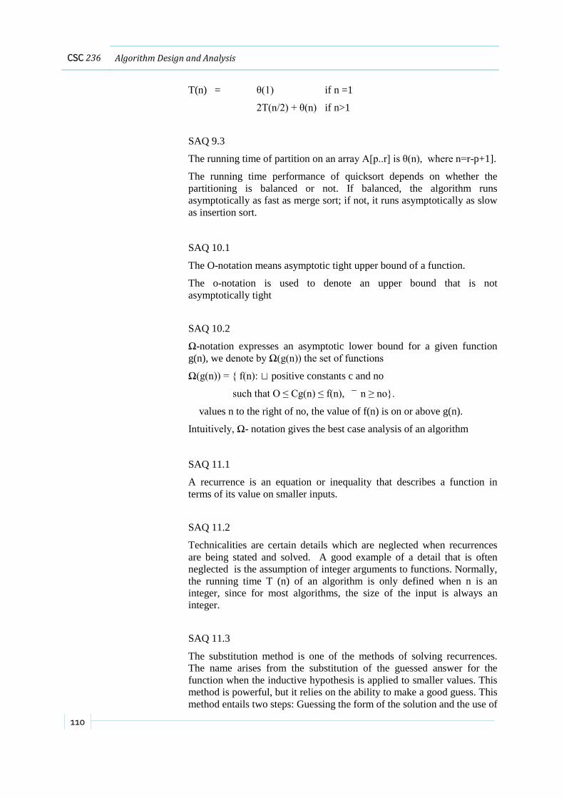
110


T(n) = θ(1) if n =1

2T(n/2) + θ(n) if n>1

SAQ 9.3

The running time of partition on an array A[p..r] is θ(n), where n=r-p+1].

The running time performance of quicksort depends on whether the

partitioning is balanced or not. If balanced, the algorithm runs

asymptotically as fast as merge sort; if not, it runs asymptotically as slow

as insertion sort.

SAQ 10.1

The O-notation means asymptotic tight upper bound of a function.

The o-notation is used to denote an upper bound that is not

asymptotically tight

SAQ 10.2

Ω-notation expresses an asymptotic lower bound for a given function

g(n), we denote by Ω(g(n)) the set of functions

Ω(g(n)) = f(n): positive constants c and no

such that O ≤ Cg(n) ≤ f(n), n ≥ no.

values n to the right of no, the value of f(n) is on or above g(n).

Intuitively, Ω- notation gives the best case analysis of an algorithm

SAQ 11.1

A recurrence is an equation or inequality that describes a function in

terms of its value on smaller inputs.

SAQ 11.2

Technicalities are certain details which are neglected when recurrences

are being stated and solved. A good example of a detail that is often

neglected is the assumption of integer arguments to functions. Normally,

the running time T (n) of an algorithm is only defined when n is an

integer, since for most algorithms, the size of the input is always an

integer.

SAQ 11.3

The substitution method is one of the methods of solving recurrences.

The name arises from the substitution of the guessed answer for the

function when the inductive hypothesis is applied to smaller values. This

method is powerful, but it relies on the ability to make a good guess. This

method entails two steps: Guessing the form of the solution and the use of


111

mathematical induction to find the constants and show that the solution

works.

SAQ 11.4

Making a good guess or guessing a solution takes experience and

sometimes creativity. The use of heuristics and recursion trees helps to

generate good guesses. Another way to make a good guess is to prove

loose upper and lower bounds on the recurrence and then reduce the

range of uncertainty.

SAQ 12.1

A recursion tree is a straightforward way to devise a good guess. In a

recursion tree, each node represents the cost of a single subproblem

somewhere in the set of recursive function invocations. We sum the costs

within each level of the tree to obtain a set of per-level costs, and then we

sum all the per-level costs to determine the total cost of all levels of the

recursion. Recursion trees are particularly useful when the recurrence

describes the running time of a divide-and-conquer algorithm. A

recursion tree is best used to generate a good guess, which is then verified

by the substitution method. You can also use a recursion tree as a direct

proof of a solution to a recurrence.

SAQ 13.1

The master method provides a "cookbook" method for solving

recurrences of the form

T(n) = aT(n/b) + f(n)

where a ≥ 1 and b > 1 are constants and f (n) is an asymptotically

positive function. The recurrence describes the running time of an

algorithm that divides a problem of size n into a subproblems, each of

size n/b, where a and b are positive constants. The a subproblems are

solved recursively, each in time T (n/b). The cost of dividing the problem

and combining the results of the subproblems is described by the function

f (n).

SAQ 13.2

The Master theorem states that let a ≥ 1 and b > 1 be constants, let f (n)

be a function, and let T (n) be defined on the nonnegative integers by the

recurrence

T(n) = aT(n/b) + f(n),

where we interpret n/b to mean either n/b or n/b . Then T (n) can

be bounded asymptotically as follows.

1. If f(n) = O(nlogba - )for some constant > 0, then T(n) =

(nlogba )

2. If f(n) = (nlogba ), then T(n) = (nlogba lgn).

112


If If f(n) = (nlogba + )for some constant > 0, and if a f (n/b) ≤ cf

(n) for some constant c < 1 and all sufficiently large n, then T (n) = Θ(f

(n)).

Documents

Algorithm Design and Analysis - School Drillers