Embed Size (px)
Citation preview

10/4/10 A. Smith; based on slides by E. Demaine, C. Leiserson, S. Raskhodnikova, K. Wayne
Adam Smith
Algorithm Design and Analysis
LECTURE 17 Dynamic Programming
• Shortest paths and
Bellman-Ford

Shortest Paths: Negative Cost Cycles
Negative cost cycle.
Observation. If some path from s to t contains a negative cost cycle,
there does not exist a shortest s-t path; otherwise, there exists one
that is simple.
s t W
c(W) < 0
-6
7
-4

Shortest Paths: Dynamic Programming
Def. OPT(i, v) = length of shortest v-t path P using at most i edges
( if no such path exists)
Case 1: P uses at most i-1 edges.
– OPT(i, v) = OPT(i-1, v)
Case 2: P uses exactly i edges.
– if (v, w) is first edge, then OPT uses (v, w), and then selects best
w-t path using at most i-1 edges
Remark. By previous observation, if no negative cycles, then
OPT(n-1, v) = length of shortest v-t path.
or
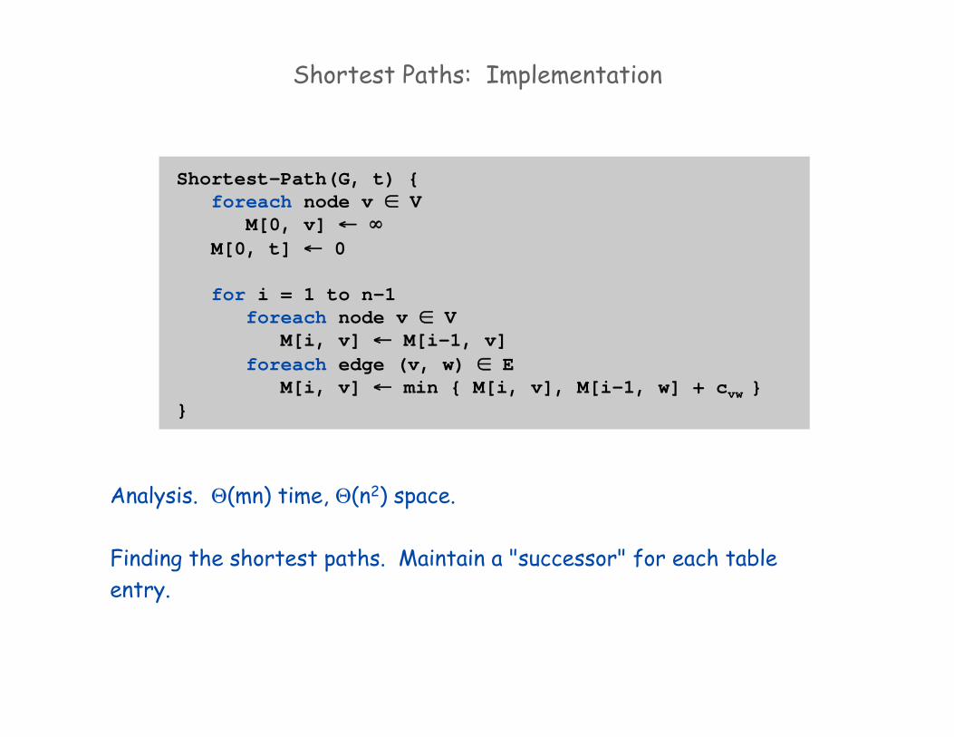
Shortest Paths: Implementation
Analysis. (mn) time, (n2) space.
Finding the shortest paths. Maintain a "successor" for each table
entry.
Shortest-Path(G, t) {
foreach node v V
M[0, v]
M[0, t] 0
for i = 1 to n-1
foreach node v V
M[i, v] M[i-1, v]
foreach edge (v, w) E
M[i, v] min { M[i, v], M[i-1, w] + cvw }
}
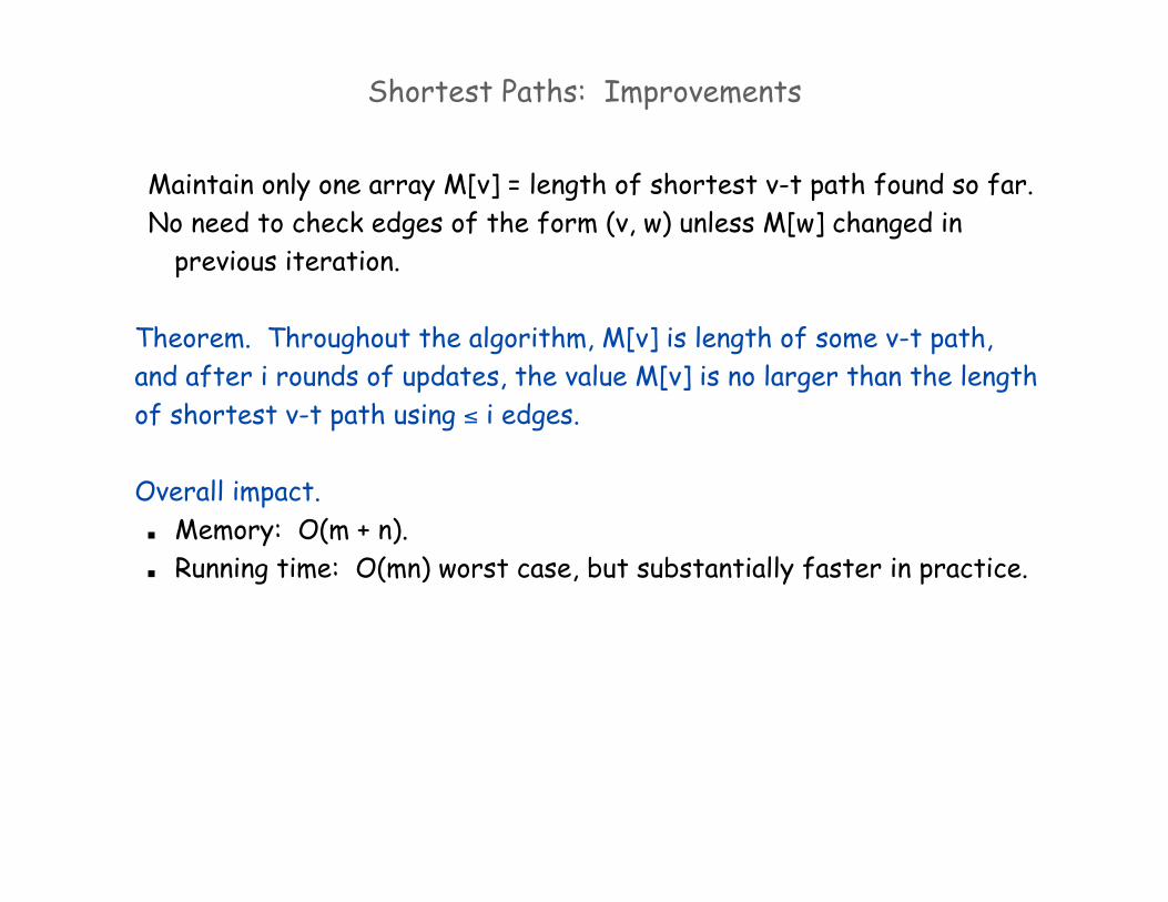
Shortest Paths: Improvements
Maintain only one array M[v] = length of shortest v-t path found so far.
No need to check edges of the form (v, w) unless M[w] changed in
previous iteration.
Theorem. Throughout the algorithm, M[v] is length of some v-t path,
and after i rounds of updates, the value M[v] is no larger than the length
of shortest v-t path using i edges.
Overall impact.
Memory: O(m + n).
Running time: O(mn) worst case, but substantially faster in practice.

Bellman-Ford: Efficient Implementation
Bellman-Ford-Shortest-Path(G, s, t) {
foreach node v V {
M[v]
successor[v]
}
M[t] = 0
for i = 1 to n-1 {
foreach node w V {
if (M[w] has been updated in previous iteration) {
foreach node v such that (v, w) E {
if (M[v] > M[w] + cvw) {
M[v] M[w] + cvw
successor[v] w
}
}
}
If no M[w] value changed in iteration i, stop.
}
}

10/4/10 A. Smith; based on slides by E. Demaine, C. Leiserson, S. Raskhodnikova, K. Wayne
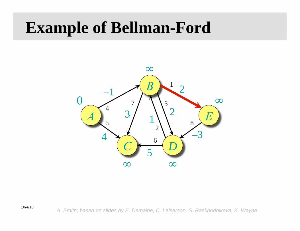
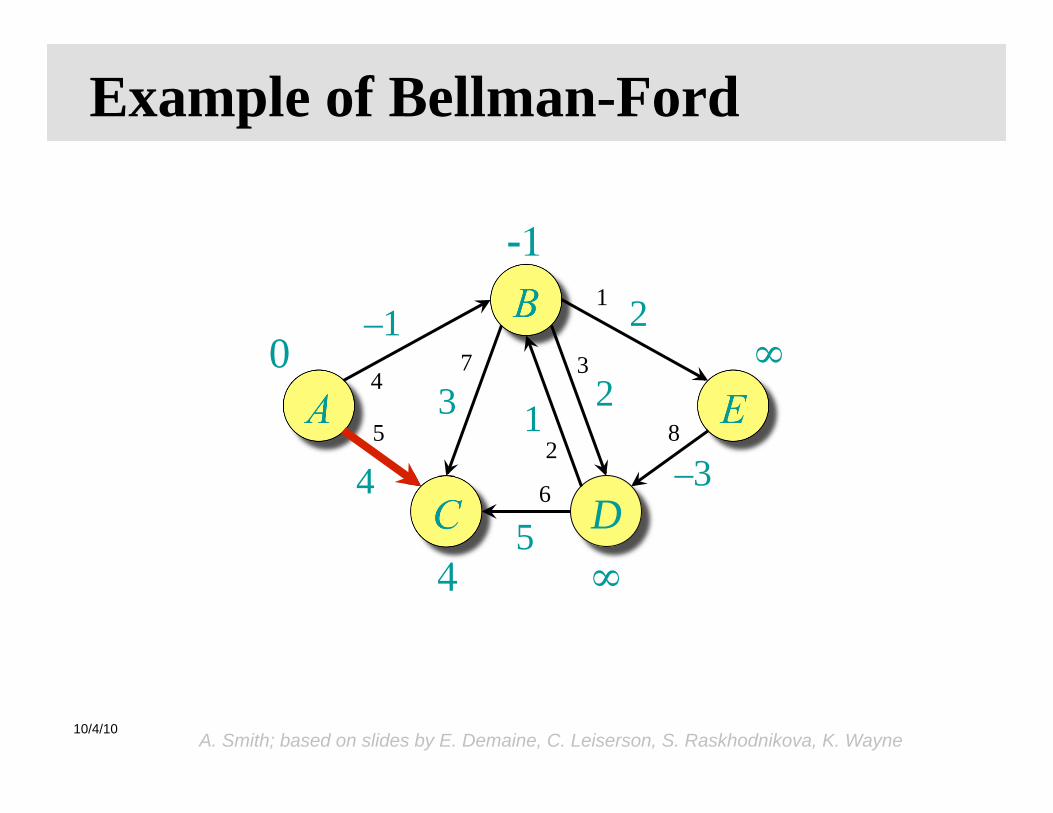
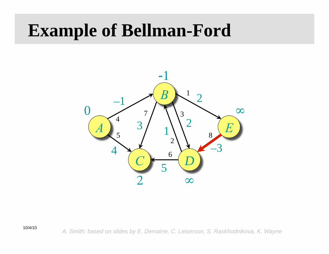
Example of Bellman-Ford
A
B
E
C D
–1
4
1 2
–3
2
5
3
The demonstration is for a sligtly different version of the algorithm (see
CLRS) that computes distances from the sourse node rather than distances to the destination node.

10/4/10 A. Smith; based on slides by E. Demaine, C. Leiserson, S. Raskhodnikova, K. Wayne
Example of Bellman-Ford
A
B
E
C D
–1
4
1 2
–3
2
5
3
0
Initialization.

10/4/10 A. Smith; based on slides by E. Demaine, C. Leiserson, S. Raskhodnikova, K. Wayne
Example of Bellman-Ford
A
B
E
C D
–1
4
1 2
–3
2
5
3
0
1
2
3 4
5
7
8
Order of edge relaxation.
6
10/4/10 A. Smith; based on slides by E. Demaine, C. Leiserson, S. Raskhodnikova, K. Wayne
Example of Bellman-Ford
A
B
E
C D
–1
4
1 2
–3
2
5
3
0
1
2
3 4
5
7
8
6

10/4/10 A. Smith; based on slides by E. Demaine, C. Leiserson, S. Raskhodnikova, K. Wayne
Example of Bellman-Ford
A
B
E
C D
–1
4
1 2
–3
2
5
3
0
1
2
3 4
5
7
8
6

10/4/10 A. Smith; based on slides by E. Demaine, C. Leiserson, S. Raskhodnikova, K. Wayne
Example of Bellman-Ford
A
B
E
C D
–1
4
1 2
–3
2
5
3
0
1
2
3 4
5
7
8
6

10/4/10 A. Smith; based on slides by E. Demaine, C. Leiserson, S. Raskhodnikova, K. Wayne
1
Example of Bellman-Ford
A
B
E
C D
–1
4
1 2
–3
2
5
3
0
1
2
3 4
5
7
8
6
10/4/10 A. Smith; based on slides by E. Demaine, C. Leiserson, S. Raskhodnikova, K. Wayne
4
1
Example of Bellman-Ford
A
B
E
C D
–1
4
1 2
–3
2
5
3
0
1
2
3 4
5
7
8
6

10/4/10 A. Smith; based on slides by E. Demaine, C. Leiserson, S. Raskhodnikova, K. Wayne
4
1
Example of Bellman-Ford
A
B
E
C D
–1
4
1 2
–3
2
5
3
0
1
2
3 4
5
7
8
6

10/4/10 A. Smith; based on slides by E. Demaine, C. Leiserson, S. Raskhodnikova, K. Wayne
42
1
Example of Bellman-Ford
A
B
E
C D
–1
4
1 2
–3
2
5
3
0
1
2
3 4
5
7
8
6
10/4/10 A. Smith; based on slides by E. Demaine, C. Leiserson, S. Raskhodnikova, K. Wayne
2
1
Example of Bellman-Ford
A
B
E
C D
–1
4
1 2
–3
2
5
3
0
1
2
3 4
5
7
8
6

10/4/10 A. Smith; based on slides by E. Demaine, C. Leiserson, S. Raskhodnikova, K. Wayne
2
1
Example of Bellman-Ford
A
B
E
C D
–1
4
1 2
–3
2
5
3
0
1
2
3 4
5
7
8
End of pass 1.
6

10/4/10 A. Smith; based on slides by E. Demaine, C. Leiserson, S. Raskhodnikova, K. Wayne
1
2
1
Example of Bellman-Ford
A
B
E
C D
–1
4
1 2
–3
2
5
3
0
1
2
3 4
5
7
8
6

10/4/10 A. Smith; based on slides by E. Demaine, C. Leiserson, S. Raskhodnikova, K. Wayne
1
2
1
Example of Bellman-Ford
A
B
E
C D
–1
4
1 2
–3
2
5
3
0
1
2
3 4
5
7
8
6

10/4/10 A. Smith; based on slides by E. Demaine, C. Leiserson, S. Raskhodnikova, K. Wayne
1
1
2
1
Example of Bellman-Ford
A
B
E
C D
–1
4
1 2
–3
2
5
3
0
1
2
3 4
5
7
8
6

10/4/10 A. Smith; based on slides by E. Demaine, C. Leiserson, S. Raskhodnikova, K. Wayne
1
1
2
1
Example of Bellman-Ford
A
B
E
C D
–1
4
1 2
–3
2
5
3
0
1
2
3 4
5
7
8
6

10/4/10 A. Smith; based on slides by E. Demaine, C. Leiserson, S. Raskhodnikova, K. Wayne
1
1
2
1
Example of Bellman-Ford
A
B
E
C D
–1
4
1 2
–3
2
5
3
0
1
2
3 4
5
7
8
6

10/4/10 A. Smith; based on slides by E. Demaine, C. Leiserson, S. Raskhodnikova, K. Wayne
1
1
2
1
Example of Bellman-Ford
A
B
E
C D
–1
4
1 2
–3
2
5
3
0
1
2
3 4
5
7
8
6

10/4/10 A. Smith; based on slides by E. Demaine, C. Leiserson, S. Raskhodnikova, K. Wayne
1
1
2
1
Example of Bellman-Ford
A
B
E
C D
–1
4
1 2
–3
2
5
3
0
1
2
3 4
5
7
8
6

10/4/10 A. Smith; based on slides by E. Demaine, C. Leiserson, S. Raskhodnikova, K. Wayne
12
1
2
1
Example of Bellman-Ford
A
B
E
C D
–1
4
1 2
–3
2
5
3
0
1
2
3 4
5
7
8
6
10/4/10 A. Smith; based on slides by E. Demaine, C. Leiserson, S. Raskhodnikova, K. Wayne
2
1
2
1
Example of Bellman-Ford
A
B
E
C D
–1
4
1 2
–3
2
5
3
0
1
2
3 4
5
7
8
6
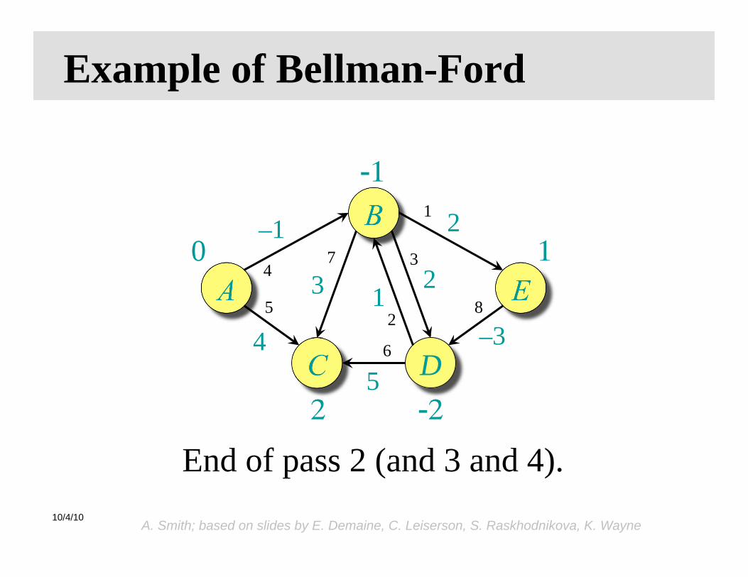
End of pass 2 (and 3 and 4).
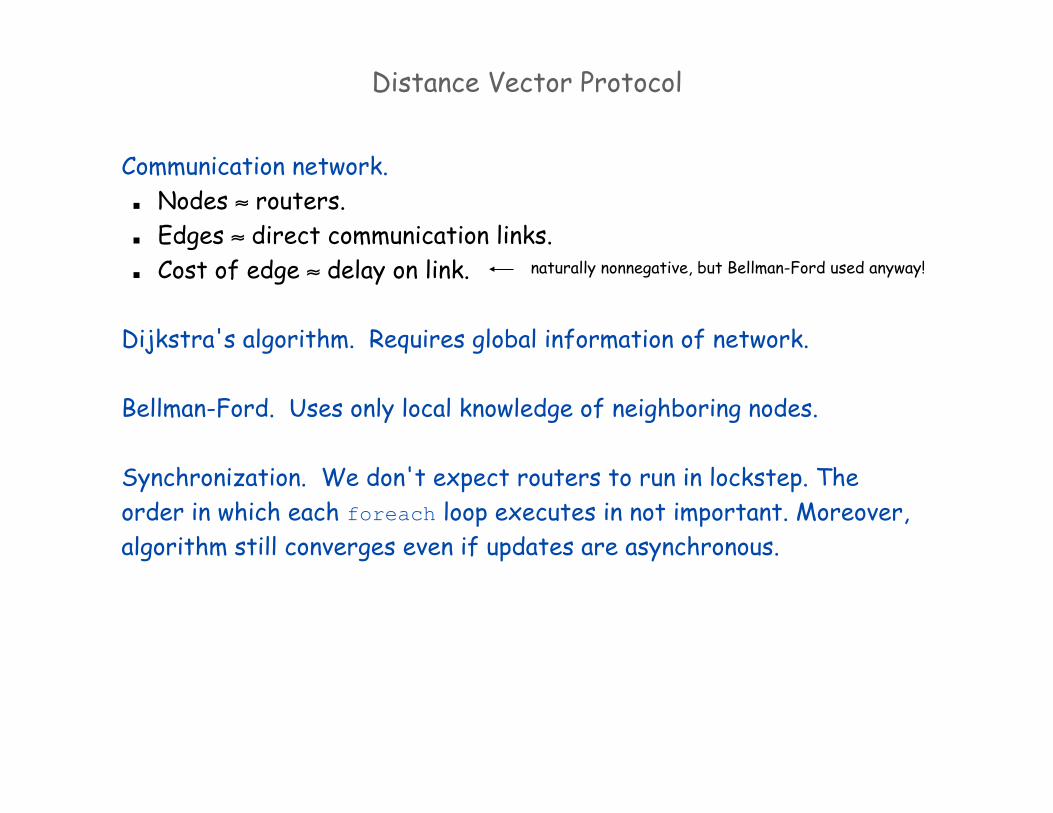
Distance Vector Protocol
Communication network.
Nodes routers.
Edges direct communication links.
Cost of edge delay on link.
Dijkstra's algorithm. Requires global information of network.
Bellman-Ford. Uses only local knowledge of neighboring nodes.
Synchronization. We don't expect routers to run in lockstep. The
order in which each foreach loop executes in not important. Moreover,
algorithm still converges even if updates are asynchronous.
naturally nonnegative, but Bellman-Ford used anyway!

Distance Vector Protocol
Distance vector protocol.
Each router maintains a vector of shortest path lengths to every
other node (distances) and the first hop on each path (directions).
Algorithm: each router performs n separate computations, one for
each potential destination node.
"Routing by rumor."
Ex. RIP, Xerox XNS RIP, Novell's IPX RIP, Cisco's IGRP, DEC's DNA
Phase IV, AppleTalk's RTMP.
Caveat. Edge costs may change during algorithm (or fail completely).
t v 1 s 1
1
deleted
"counting to infinity"
2 1

Path Vector Protocols
Link state routing.
Each router also stores the entire path.
Based on Dijkstra's algorithm.
Avoids "counting-to-infinity" problem and related difficulties.
Requires significantly more storage.
Ex. Border Gateway Protocol (BGP), Open Shortest Path First (OSPF).
not just the distance and first hop
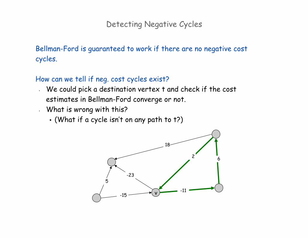
Detecting Negative Cycles
Bellman-Ford is guaranteed to work if there are no negative cost
cycles.
How can we tell if neg. cost cycles exist?
• We could pick a destination vertex t and check if the cost
estimates in Bellman-Ford converge or not.
• What is wrong with this?
• (What if a cycle isn’t on any path to t?)
v
18
2
5 -23
-15 -11
6

Detecting Negative Cycles
Theorem. Can find negative cost cycle in O(mn) time.
Add new node t and connect all nodes to t with 0-cost edge.
Check if OPT(n, v) = OPT(n-1, v) for all nodes v.
– if yes, then no negative cycles
– if no, then extract cycle from shortest path from v to t
v
18
2
5 -23
-15 -11
6
t
0
0
0 0
0
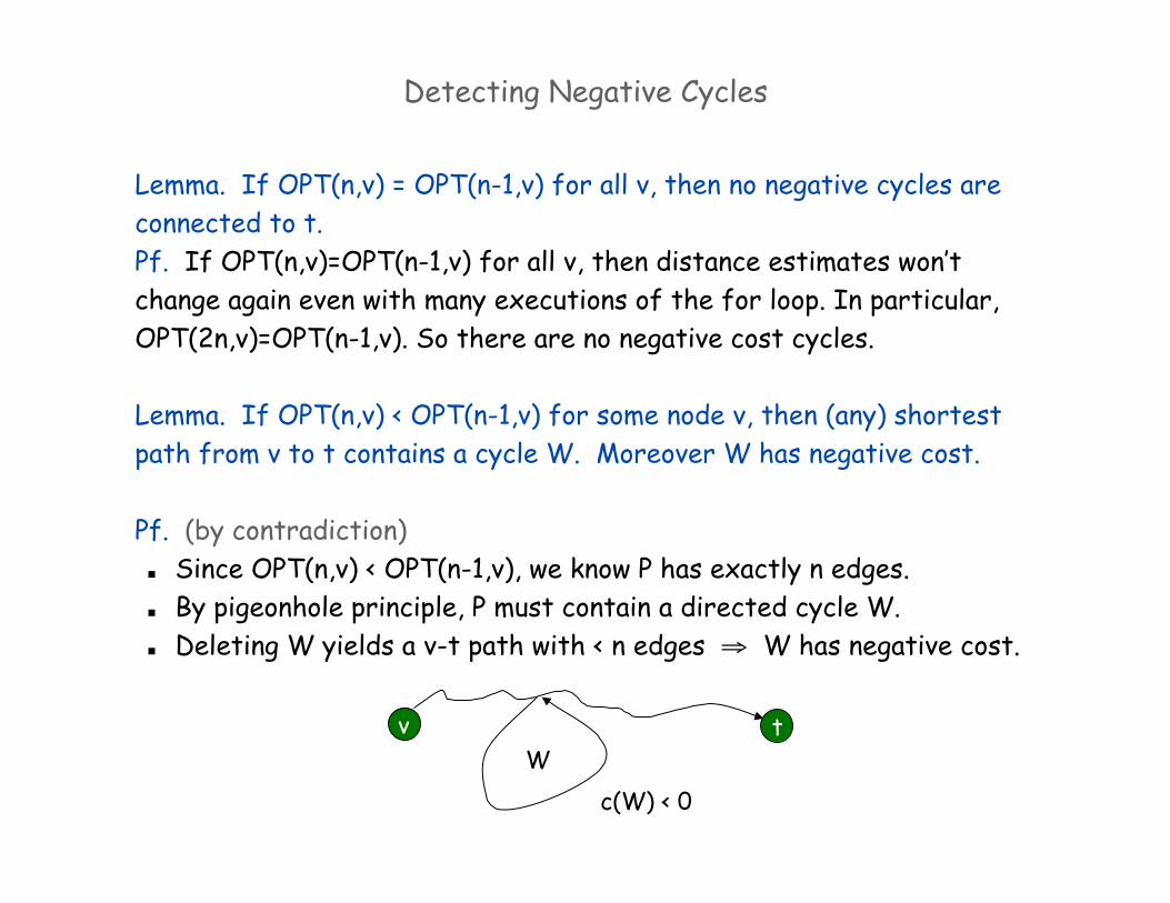
Detecting Negative Cycles
Lemma. If OPT(n,v) = OPT(n-1,v) for all v, then no negative cycles are
connected to t.
Pf. If OPT(n,v)=OPT(n-1,v) for all v, then distance estimates won’t
change again even with many executions of the for loop. In particular,
OPT(2n,v)=OPT(n-1,v). So there are no negative cost cycles.
Lemma. If OPT(n,v) < OPT(n-1,v) for some node v, then (any) shortest
path from v to t contains a cycle W. Moreover W has negative cost.
Pf. (by contradiction)
Since OPT(n,v) < OPT(n-1,v), we know P has exactly n edges.
By pigeonhole principle, P must contain a directed cycle W.
Deleting W yields a v-t path with < n edges W has negative cost.
v t W
c(W) < 0

Detecting Negative Cycles: Application
Currency conversion. Given n currencies and exchange rates between
pairs of currencies, is there an arbitrage opportunity?
Remark. Fastest algorithm very valuable!
F $
£ ¥ DM
1/7
3/10 2/3 2
170 56
3/50 4/3
8
IBM
1/10000
800

Detecting Negative Cycles: Summary
Bellman-Ford. O(mn) time, O(m + n) space.
Run Bellman-Ford for n iterations (instead of n-1).
Upon termination, Bellman-Ford successor variables trace a negative
cycle if one exists.
See p. 304 for improved version and early termination rule.