Embed Size (px)
Citation preview
Alireza Salehi Golsefidy
Algebra: ring and field theory


Contents
Contents 3
1 Lecture 1 91.1 Introduction: a pseudo-historical note . . . . . . . . . . . . . . . . . 91.2 Rings: definition and basic examples. . . . . . . . . . . . . . . . . . 101.3 Basic properties of operations in a ring. . . . . . . . . . . . . . . . . 121.4 Subring and homomorphism. . . . . . . . . . . . . . . . . . . . . . . 13
2 Lecture 2 152.1 More on subrings and ring homomorphisms. . . . . . . . . . . . . . . 152.2 Kernel and image of a ring homomorphism. . . . . . . . . . . . . . . 162.3 A special ring homomorphism . . . . . . . . . . . . . . . . . . . . . 172.4 The evaluation or the substitution map . . . . . . . . . . . . . . . . . 19
3 Lecture 3 213.1 The evaluation or the substitution map . . . . . . . . . . . . . . . . . 213.2 Units and fields . . . . . . . . . . . . . . . . . . . . . . . . . . . . . 223.3 Zero-divisors and integral domains . . . . . . . . . . . . . . . . . . . 243.4 Characteristic of a unital ring . . . . . . . . . . . . . . . . . . . . . . 25
4 Lecture 4 274.1 Defining fractions . . . . . . . . . . . . . . . . . . . . . . . . . . . . 274.2 Defining addition and multiplication of fractions . . . . . . . . . . . . 284.3 Fractions form a field . . . . . . . . . . . . . . . . . . . . . . . . . . 294.4 The universal property of the field of fractions . . . . . . . . . . . . . 29
5 Lecture 5 335.1 Using the universal property of the field of fractions. . . . . . . . . . 335.2 Ideals . . . . . . . . . . . . . . . . . . . . . . . . . . . . . . . . . . 345.3 Quotient rings . . . . . . . . . . . . . . . . . . . . . . . . . . . . . . 355.4 The first isomorphism theorem for rings . . . . . . . . . . . . . . . . 37
6 Lecture 6 396.1 An application of the first isomorphism theorem. . . . . . . . . . . . 396.2 Degree of polynomials . . . . . . . . . . . . . . . . . . . . . . . . . 40
3

4 CONTENTS
6.3 Zero-divisors and units of ring of polynomials . . . . . . . . . . . . . 416.4 Long division . . . . . . . . . . . . . . . . . . . . . . . . . . . . . . 42
7 Lecture 7 457.1 The factor theorem and the generalized factor theorems . . . . . . . . 457.2 An application of the generalized factor theorem . . . . . . . . . . . . 477.3 Ideals of ring of polynomials over a field . . . . . . . . . . . . . . . . 487.4 Euclidean Domain . . . . . . . . . . . . . . . . . . . . . . . . . . . 49
8 Lecture 8 518.1 Gaussian integers . . . . . . . . . . . . . . . . . . . . . . . . . . . . 518.2 Algebraic elements and minimal polynomials . . . . . . . . . . . . . 528.3 Elements of quotients of ring of polynomials . . . . . . . . . . . . . . 54
9 Lecture 9 579.1 Elements of F [α] . . . . . . . . . . . . . . . . . . . . . . . . . . . . 579.2 Irreducible elements . . . . . . . . . . . . . . . . . . . . . . . . . . 589.3 Maximal ideals and their quotient rings . . . . . . . . . . . . . . . . 619.4 F [α] is a field! . . . . . . . . . . . . . . . . . . . . . . . . . . . . . 62
10 Lecture 10 6310.1 Irreducibility and zeros of polynomials . . . . . . . . . . . . . . . . . 6310.2 Rational root criterion . . . . . . . . . . . . . . . . . . . . . . . . . . 6410.3 Mod criterion: zeros . . . . . . . . . . . . . . . . . . . . . . . . . . 65
11 Lecture 11 6711.1 Content of a polynomial with rational coefficients. . . . . . . . . . . . 6711.2 Gauss’s lemma . . . . . . . . . . . . . . . . . . . . . . . . . . . . . 6911.3 Factorization: going from rationals to integers. . . . . . . . . . . . . 7011.4 Mod criterion: irreducibility . . . . . . . . . . . . . . . . . . . . . . 71
12 Lecture 12 7312.1 An example on the mod irreducibility criterion. . . . . . . . . . . . . 7312.2 Eisenstein’s irreducibility criterion . . . . . . . . . . . . . . . . . . . 7412.3 Factorization: existence, and a chain condition . . . . . . . . . . . . . 76
13 Lecture 13 7913.1 Factorization: uniqueness, and prime elements. . . . . . . . . . . . . 7913.2 Prime elements and prime ideals . . . . . . . . . . . . . . . . . . . . 8113.3 Prime vs irreducible . . . . . . . . . . . . . . . . . . . . . . . . . . . 8213.4 Some integral domains that are not UFD. . . . . . . . . . . . . . . . 83
14 Lecture 14 8514.1 Ring of integer polynomials is a UFD. . . . . . . . . . . . . . . . . . 85
15 Lecture 15 8915.1 Valuations and greatest common divisors in a UFD . . . . . . . . . . 89
CONTENTS 5
15.2 Greatest common divisor for UFDs . . . . . . . . . . . . . . . . . . . 9315.3 Content of polynomials: UFD case . . . . . . . . . . . . . . . . . . . 9315.4 Gauss’s lemma for UFDs. . . . . . . . . . . . . . . . . . . . . . . . . 95
16 Lecture 16 9716.1 Existence of a splitting field. . . . . . . . . . . . . . . . . . . . . . . 9716.2 Towards uniqueness of a splitting field. . . . . . . . . . . . . . . . . . 100
17 Lecture 17 10317.1 Extension of isomorphisms to splitting fields. . . . . . . . . . . . . . 10317.2 Two examples . . . . . . . . . . . . . . . . . . . . . . . . . . . . . . 106
18 Lecture 18 10718.1 Finite fields: uniqueness . . . . . . . . . . . . . . . . . . . . . . . . 10818.2 Finite fields: towards existence . . . . . . . . . . . . . . . . . . . . . 10918.3 Separability: having distinct zeros in a splitting field. . . . . . . . . . 11018.4 Finite field: existence . . . . . . . . . . . . . . . . . . . . . . . . . . 112
19 Lecture 19 11319.1 Vector spaces over a field . . . . . . . . . . . . . . . . . . . . . . . . 11319.2 Subspace and linear map . . . . . . . . . . . . . . . . . . . . . . . . 11519.3 Dimension of a vector space . . . . . . . . . . . . . . . . . . . . . . 11719.4 Quotient spaces . . . . . . . . . . . . . . . . . . . . . . . . . . . . . 11819.5 The first isomorphism theorem for vector spaces . . . . . . . . . . . . 121
20 Lecture 20 12320.1 Previous results in the language of linear algebra . . . . . . . . . . . . 12320.2 Finite fields and vector spaces . . . . . . . . . . . . . . . . . . . . . 12420.3 Tower rule for field extensions . . . . . . . . . . . . . . . . . . . . . 12420.4 Some applications of the Tower Rule for field extensions . . . . . . . 12620.5 Algebraic closure in a field extension . . . . . . . . . . . . . . . . . . 12820.6 Tower of algebraic extensions . . . . . . . . . . . . . . . . . . . . . . 12820.7 Geometric constructions by ruler and compass . . . . . . . . . . . . . 129
21 Lecture 21 13121.1 Cyclotomic polynomials . . . . . . . . . . . . . . . . . . . . . . . . 13121.2 Cyclotomic polynomials are integer polynomials . . . . . . . . . . . . 13221.3 Cyclotomic polynomials are irreducible . . . . . . . . . . . . . . . . 13421.4 The degree of cyclotomic extensions . . . . . . . . . . . . . . . . . . 135
22 Lecture 22 13722.1 The group of automorphism of a field extension. . . . . . . . . . . . . 13722.2 Normal extensions . . . . . . . . . . . . . . . . . . . . . . . . . . . 138
23 Lecture 23 14323.1 The group of automorphism of normal field extensions. . . . . . . . . 14323.2 Normal extensions and tower of fields . . . . . . . . . . . . . . . . . 144
6 CONTENTS
23.3 Normal closure of a field extension . . . . . . . . . . . . . . . . . . . 14523.4 Normal extension and extending embeddings . . . . . . . . . . . . . 14623.5 Group of automorphisms of a field extension . . . . . . . . . . . . . . 146
24 Lecture 24 14924.1 Separable polynomials . . . . . . . . . . . . . . . . . . . . . . . . . 14924.2 Separable and Galois extensions . . . . . . . . . . . . . . . . . . . . 150
25 Lecture 1 15325.1 Review . . . . . . . . . . . . . . . . . . . . . . . . . . . . . . . . . 15325.2 Symmetries and field extensions . . . . . . . . . . . . . . . . . . . . 15525.3 Finite Galois extensions and orbits of their symmetries . . . . . . . . 15725.4 Subgroups and intermediate subfields . . . . . . . . . . . . . . . . . 158
26 Lecture 2 16126.1 Fixed points of a subgroup. . . . . . . . . . . . . . . . . . . . . . . . 16126.2 Fundamental Theorem of Galois Theory . . . . . . . . . . . . . . . . 164
27 Lecture 3 16927.1 Fundamental theorem of algebra . . . . . . . . . . . . . . . . . . . . 16927.2 Primitive Element Theorem . . . . . . . . . . . . . . . . . . . . . . . 17027.3 Separable closure of the base field of an algebraic extension . . . . . . 172
28 Lecture 4 17728.1 Purely inseparable extensions . . . . . . . . . . . . . . . . . . . . . . 17728.2 Block-Tower Phenomena for separable extensions . . . . . . . . . . . 17828.3 Solvability by radicals . . . . . . . . . . . . . . . . . . . . . . . . . . 179
29 Lecture 5 18329.1 Radical extensions . . . . . . . . . . . . . . . . . . . . . . . . . . . 18329.2 Solvable by radicals . . . . . . . . . . . . . . . . . . . . . . . . . . . 185
30 Lecture 6 18930.1 Basics of solvable groups . . . . . . . . . . . . . . . . . . . . . . . . 18930.2 Galois groups and permutations . . . . . . . . . . . . . . . . . . . . 19130.3 Examples of polynomials that are not solvable by radicals . . . . . . . 19230.4 Finite solvable groups and prime order factors . . . . . . . . . . . . . 193
31 Lecture 7 19731.1 A tower of cyclic Galois extensions with roots of unity . . . . . . . . 19731.2 Hilbert’s theorem 90 . . . . . . . . . . . . . . . . . . . . . . . . . . 19831.3 Cyclic extensions with enough roots of unity . . . . . . . . . . . . . . 20231.4 Completing proof of Galois’s solvability theorem . . . . . . . . . . . 203
32 Lecture 8 20532.1 Algebraically closed fields . . . . . . . . . . . . . . . . . . . . . . . 20532.2 Zorn’s lemma . . . . . . . . . . . . . . . . . . . . . . . . . . . . . . 206
CONTENTS 7
32.3 Maximal ideals . . . . . . . . . . . . . . . . . . . . . . . . . . . . . 20832.4 Existence of algebraic closure: one zero of every polynomial . . . . . 209
33 Lecture 9 21133.1 Existence of an algebraic closure . . . . . . . . . . . . . . . . . . . . 21133.2 Isomorphism extension theorem for algebraic closures. . . . . . . . . 21233.3 Basic properties of algebraic closures . . . . . . . . . . . . . . . . . 21433.4 Group of automorphisms of algebraic closures . . . . . . . . . . . . . 216
34 Lecture 10 21934.1 Galois correspondence for algebraic closures . . . . . . . . . . . . . 21934.2 Statement of the cyclic case of Kummer theory and pairing . . . . . . 22134.3 Functions in the cyclic case of Kummer theory . . . . . . . . . . . . 223
35 Lecture 11 22535.1 Kummer theory: the cyclic case . . . . . . . . . . . . . . . . . . . . 22535.2 Dual of abelian groups . . . . . . . . . . . . . . . . . . . . . . . . . 226
36 Lecture 12 23136.1 Dual of abelian groups . . . . . . . . . . . . . . . . . . . . . . . . . 23136.2 Statement of finite abelian case of Kummer theory . . . . . . . . . . . 23336.3 Kummer pairing is a perfect pairing . . . . . . . . . . . . . . . . . . 23536.4 Perfect pairings . . . . . . . . . . . . . . . . . . . . . . . . . . . . . 23736.5 Proof of Kummer theory: abelian case . . . . . . . . . . . . . . . . . 238
37 Lecture 13 23937.1 Module theory: basic examples . . . . . . . . . . . . . . . . . . . . . 23937.2 The first isomorphism theorem . . . . . . . . . . . . . . . . . . . . . 24137.3 Noetherian modules . . . . . . . . . . . . . . . . . . . . . . . . . . . 243
38 Lecture 14 24738.1 Noetherian modules . . . . . . . . . . . . . . . . . . . . . . . . . . . 24738.2 Finitely generated modules and cokernel of matrices . . . . . . . . . 25138.3 Reduced row/column operations, Smith normal form. . . . . . . . . . 252
39 Lecture 15 25939.1 Finitely generated modules over a Euclidean Domain . . . . . . . . . 25939.2 Finitely generated abelian groups . . . . . . . . . . . . . . . . . . . . 26039.3 Linear transformations and matrices . . . . . . . . . . . . . . . . . . 26139.4 Linear maps, evaluation map, and minimal polynomial . . . . . . . . 264
40 Lecture 16 26740.1 Linear maps, evaluation map, module structure . . . . . . . . . . . . 26740.2 Reduction to the cyclic case. . . . . . . . . . . . . . . . . . . . . . . 26840.3 Cyclic case, companion matrix, and rational canonical form . . . . . . 26940.4 The Cayley-Hamilton Theorem . . . . . . . . . . . . . . . . . . . . . 271
8 CONTENTS
41 Lecture 17 27541.1 Generalized long division . . . . . . . . . . . . . . . . . . . . . . . . 27641.2 Hilbert’s basis theorem . . . . . . . . . . . . . . . . . . . . . . . . . 27941.3 Finitely generated rings and algebras . . . . . . . . . . . . . . . . . . 280
42 Lectures 18 and 19 28342.1 Set of common zeros and vanishing polynomials . . . . . . . . . . . . 28342.2 Our general approach for finding a solution . . . . . . . . . . . . . . 28442.3 Resultant of two polynomials . . . . . . . . . . . . . . . . . . . . . . 28642.4 What happens if π is not surjective . . . . . . . . . . . . . . . . . . . 28842.5 Finding a suitable linear change of coordinates . . . . . . . . . . . . . 28942.6 Hilbert’s Nullstellensatz . . . . . . . . . . . . . . . . . . . . . . . . . 29142.7 Final remarks . . . . . . . . . . . . . . . . . . . . . . . . . . . . . . 295

Chapter 1
Lecture 1
In this lecture, we start with a pseudo-historical note on algebra. Next ring is definedand some examples are briefly mentioned. Ring of polynomials and direct product ofrings are discussed. Then basic properties of ring operations are discussed. At the end,we define subrings, ring homomorphism, and ring isomorphism
1.1 Introduction: a pseudo-historical note
A large part of algebra has been developed to systematically study zeros of polyno-mials. The word algebra comes from the name of a book by al-Khwarizmi, a Persianmathematician, 1 where al-Khwarizmi essentially gave algorithms to find zeros oflinear and quadratic equations. Khayyam, another Persian mathematician, made majoradvances in understanding of zeros of cubic equations. In the 16th century, Italianmathematicians came up with formulas for zeros of general cubic and quartic equations.The cubic case was solved by del Ferro, and Ferrari solved the quartic case.2 In 1824,Abel proved that there is no solutions in radicals to a general polynomial equation ofdegree at least 5. In 1832, Galois used symmetries (group theory) of system of numbersof zeros of a polynomial to systematically study them, and he gave the precise conditionunder which solutions can be written using radicals (and the usual operations +,−, ·, /).
Another problem which had a great deal of influence on shaping modern algebra isFermat’s last conjecture: there are no positive integers x, y, z such that xn + yn = zn
if n is an integer more than 2. As you can see this problem has two new directions:
1. it is a multi-variable equation,
2. it is a Diophantine equation. This means we are looking for integer solutionsinstead of complex or real solutions.
The first direction was important in the development of the algebraic geometry, and thesecond one was played a crucial role in the development of algebraic number theory.
1I am Persian, and so I have to start with this!2In the book A History of Algebra; from al-Khwarizmi to Emmy Noether, by van der Waerden, you can
read about the very interesting history of the solution of cubic equations by del Ferro, Tartaglia, and Cardano.
9

10 CHAPTER 1. LECTURE 1
In this course, I often try to put what we learn in the perspective of these pseudo-historical remarks.
1.2 Rings: definition and basic examples.
As we mentioned earlier, our hidden agenda is to understand zeros of a polynomial.Say p(x) is a polynomial with rational coefficients. We would like to understandproperties of a zero α ∈ C of p(x). What exactly does understanding mean here?Whatever it means, we would expect to be able to do basic arithmetic with α: add andmultiply, and find out if we are getting the same values or not. As we see later, thismeans we want to understand various properties of the subring of C that is generatedby α.
Definition 1.2.1. 1. A ring (R,+, ·) is a set R with two binary operations: +(addition) and · (multiplication) such that the following holds:
(i) (R,+) is an abelian group.
(ii) (Associative) For every a, b, c ∈ R, a · (b · c) = (a · b) · c.
(iii) (Distributive) For every a, b, c ∈ R,
a · (b+ c) = a · b+ a · c and (b+ c) · a = b · a+ c · a.
2. We say R is a unital ring if there is 1 ∈ R such that 1 · a = a · 1 for every a ∈ R.
3. We say R is a commutative ring if a · b = b · a for every a, b ∈ R.
Basic examples.The set Z of integers, the set Q of rational numbers, the set R of real numbers, and
the set C of complex numbers are unital commutative rings.Some non-examples.The set of non-negative integers Z≥0 is not a ring as (Z≥0,+) is not an abelian
group.The set of even integers 2Z is a commutative ring, but it is not unital.For an integer n more than 1, the set Mn(R) of n-by-n matrices with real entries is
a unital ring, but it is not commutative. In fact, for every ring R and positive integer n,the set Mn(R) of n-by-n matrices with entries in R with the usual matrix addition andmultiplication forms a ring. Moreover, if R is unital, then Mn(R) is also unital.
Ring of integers modulo n.
The set Zn of integers modulo n is another important ring. Let us recall that theresidue class [a]n of a modulo n consists all the integers of the form nk + a where kis an integer. In group theory, you have learned that Zn = {[0]n, . . . , [n − 1]n} canbe identified with the quotient group Z/nZ, and the residue class [a]n of a modulo n

1.2. RINGS: DEFINITION AND BASIC EXAMPLES. 11
is precisely the coset a+ nZ of the (normal) subgroup nZ. Let us also recall that forevery a, a′, b, b′ ∈ Z and positive integer n the following holds:
a ≡ a′ (mod n)b ≡ b′ (mod n)
}⇒ aa′ ≡ bb′ (mod n).
This implies that the following is a well-defined binary operator on Zn:
[a]n · [b]n := [ab]n
for every a and b in Z. It is easy to check that (Zn,+, ·) is a unital commutative ring.
Exercise 1.2.2. Work out the details of why Zn is a ring.
Ring of Polynomials.
As we have mentioned earlier, polynomials play an indispensable role in algebra.Notice that we can and will work with polynomials with coefficients in an arbitraryring R. The set of all polynomials with coefficients in a ring R and an indeterminant xis denoted by R[x]. Therefore
R[x] := {anxn + · · ·+ a0| n ∈ Z≥0, a0, . . . , an ∈ R}.
We sometimes write∑ni=0 aix
i instead of anxn+· · ·+a0. In some arguments it is moreconvenient to write a polynomial as an infinite sum
∑∞i=0 aix
i with an understandingthat an+1 = an+2 = · · · = 0 for some non-negative integer n. Based on our experienceof working with polynomials with real or complex coefficients, we define the followingoperations:( ∞∑
i=0
aixi)
+( ∞∑i=0
bixi)
:=
∞∑i=0
(ai + bi)xi (addition)
( ∞∑i=0
aixi)( ∞∑
i=0
bixi)
:=
∞∑n=0
( n∑i=0
aibn−i)xn (multiplication)
for every∑∞i=0 aix
i,∑∞i=0 bix
i ∈ R[x]. It is easy to see that (R[x],+, ·) is a ring.
Example 1.2.3. Compute ([2]4x+ [1]4)([2]4x2 + [3]4x+ [1]4) in Z4[x].
Solution. We start the computation as if the coefficients were real numbers and use thedistribution law. Moreover to simplify our notation, we drop the decoration [ ]4, but weremember that computation of coefficients should be done in Z4. Hence:
([2]4x+ [1]4)([2]4x2 + [3]4x+ [1]4)
= (2 · 2)x3 + (2 · 3 + 1 · 2)x2 + (2 · 1 + 1 · 3)x+ (1 · 1)
= x+ 1.
12 CHAPTER 1. LECTURE 1
Exercise 1.2.4. 1. Compute (x+ 1)3 in Z3[x].
2. Suppose p is prime. Compute (x+ 1)p in Zp[x].
(Hint. By the binomial expansion the coefficient of xi in (x+ 1)p is(pi
). Argue
why(pi
)is zero in Zp if 1 ≤ i ≤ p− 1.)
Warning. Prior to this course, you have viewed a polynomial f ∈ R[x] as a functionfrom R to R. There is, however, a subtle difference between polynomials and functions.For instance, x, x2, . . . are distinct elements of Z2[x], but all of them are the samefunctions from Z2 to Z2. Notice that two polynomials
∑∞i=0 aix
i and∑∞i=0 bix
i areequal if and only if ai = bi for every non-negative integer i.
Nevertheless, later we will see that viewing polynomials as functions is extremelyuseful.
Direct product of rings
Suppose R1, . . . , Rn are rings. Then the set
R1 × · · · ×Rn := {(r1, . . . , rn)| r1 ∈ R1, . . . , rn ∈ Rn}
with operations
(r1, . . . , rn) + (r′1, . . . , r′n) :=(r1 + r′1, . . . , rn + r′n)
(r1, . . . , rn) · (r′1, . . . , r′n) :=(r1 · r′1, . . . , rn · r′n)
is a ring, and it is called the direct product of Ri’s. Notice the operations in the i-thcomponent are done in Ri.
Example 1.2.5. Compute (2, 2) · (3, 3) in Z5 × Z6.
Solution. We notice that 2 · 3 = 1 in Z5 and 2 · 3 = 0 in Z6. Hence we have(2, 2) · (3, 3) = (1, 0) in Z5 × Z6.
1.3 Basic properties of operations in a ring.
Here we see that some basic computations hold in every ring, and a unital ring Rhas a unique identity, which is sometimes denoted by 1R.
Lemma 1.3.1. Suppose R is a ring and 0 is the neutral element of the abelian group(R,+). Then for every a, b ∈ R, the following hold:
1. 0 · a = a · 0 = 0.
2. (−a) · b = −(a · b) = a · (−b).
3. (−a) · (−b) = a · b.

1.4. SUBRING AND HOMOMORPHISM. 13
Proof. (1) Since 0 = 0 + 0, we have 0 · a = (0 + 0) · a for every a ∈ R. Hence by thedistribution law, we have
0 · a = (0 · a) + (0 · a).
As (R,+) is a group, we deduce that 0 = 0 · a. Similarly we have
a · 0 = a · (0 + 0) = (a · 0) + (a · 0), which implies that 0 = a · 0.
(2) To show (−a) · b = −(a · b), we need to argue why (a · b) + ((−a) · b) = 0 :
(a · b) + ((−a) · b) =(a+ (−a)) · b (distribution law)=0 · b=0 (by the first part).
By a similar argument, we can deduce that a · (−b) = −(a · b).(3) Using the second part twice, we obtain the last part as follows:
(−a) · (−b) = −(a · (−b)) = −(−(a · b)) = a · b.
This finishes the proof.
Lemma 1.3.2. Suppose R is a unital ring. Then there is a unique element 1R ∈ Rsuch that
1R · a = a · 1R = a (1.1)
for every a ∈ R.
Proof. Suppose both 1 and 1′ satisfy (1.1). Then
1 =1 · 1′ (as 1′ satisfies (1.1))=1′ (as 1 satisfies (1.1)),
and the claim follows.
Exercise 1.3.3. SupposeR1, . . . , Rn are unital rings. Show that (1R1 , . . . , 1Rn) is theidentity of R1 × · · · ×Rn.
1.4 Subring and homomorphism.
Whenever you learn a new structure, you should look for subsets that share the sameproperties (they are often called sub-), and more importantly maps that preserves thoseproperties (they are often called homomorphisms).
Definition 1.4.1. Suppose (R,+, 0) is a ring. A subset S of R is called a subring of Rif
1. (S,+) is a subgroup of (R,+).
2. S is closed under multiplication. This means that for every a, b ∈ S, we haveab ∈ S.

14 CHAPTER 1. LECTURE 1
Warning In your book, having an identity is part of the definition of a ring. As aresult a subring of a ring R should contain the identity of R. In our course, we do notmake that assumption for subrings.
Example 1.4.2. Z is a subring of Q. Q is a subring of R. R is a subring of C.
Exercise 1.4.3. 1. What is the smallest subring of C that contains Q and i?
2. What is the smallest subring of C that contains Q and√
2?
3. What is the smallest subring of C that contains Q and 3√
2?
Definition 1.4.4. Suppose R1 and R2 are two rings. Then a function f : R1 → R2 iscalled a ring homomorphism if for every a, b ∈ R1
1. f(a+ b) = f(a) + f(b),
2. f(a · b) = f(a) · f(b).
Warning As it has been mentioned earlier, in your book, having an identity is partof the definition of a ring. As a result a ring homomorphism between two rings A andB should send 1A to 1B . In this course, we refer to the ring homomorphisms that send1A to 1B as unital ring homomorphisms.
Example 1.4.5. For every positive integer n, cn : Z → Zn, cn(a) := [a]n is a ringhomomorphism.

Chapter 2
Lecture 2
In this lecture, first we show the subring criterion and present important ringhomomorphisms. Next we define the kernel and the image of a ring homomorphism.The third topic is on the group of units of a ring, and the definition of a field. As animportant example, we find the group of units of the ring of integers modulo n. Finallywe define zero-divisors and integral domains.
2.1 More on subrings and ring homomorphisms.
We start by defining a ring isomorphism.
Lemma 2.1.1. Suppose f : R1 → R2 is a bijective ring homomorphism. Thenf−1 : R2 → R1 is a ring homomorphism.
Proof. Since f is a bijection, it is invertible and there is the function f−1 : R2 → R1.For every a, b ∈ R2, we have
f(f−1(a) + f−1(b)) =f(f−1(a)) + f(f−1(b))
=a+ b.
Hence f−1(a+ b) = f−1(a) + f−1(b). Similarly we have
f(f−1(a) · f−1(b)) =f(f−1(a)) · f(f−1(b))
=a · b.
Hence f−1(a · b) = f−1(a) · f−1(b). The claim follows.
Definition 2.1.2. A bijective ring homomorphism is called a ring isomorphism. Wesay two rings are isomorphic if there is a ring isomorphism between them.
As in group theory, two isomorphic rings are essentially the same with differentlabelling!
Let us start with subgroup criterion from group theory.
15

16 CHAPTER 2. LECTURE 2
Lemma 2.1.3 (Subgroup criterion). Suppose (G, ·) is a group and H is a non-emptysubset. If for every h, h′ ∈ H , we have hh′−1 ∈ H , then H is a subgroup.
We can use the subgroup criterion in order to show the subring criterion.
Lemma 2.1.4 (Subring criterion). Suppose R is a ring and S is a non-empty subset ofR. If for every a, b ∈ S, we have
1. a− b ∈ S, and
2. a · b ∈ S,
then S is a subring.
Proof. By the subgroup criterion, we deduce that (S,+) is a subgroup of (R,+). SinceS is also closed under multiplication, we deduce that S is a subring.
2.2 Kernel and image of a ring homomorphism.
A good application of the subring criterion is to show that the kernel of a ringhomomorphism and its image are subrings. Let us recall from group theory that thekernel of a group homomorphism f between two abelian groups A1 and A2 is
ker f := {a ∈ A1| f(a1) = 0},
and ker f is a subgroup of A1. We also have that the image of f is
Im f := {f(a)| a ∈ A1},
and it is a subgroup of A2. Since a ring homomorphism f is also an additive grouphomomorphism, we deduce that ker f and Im f are subgroups of the domain of f andthe codomain of f , respectively.
Lemma 2.2.1. Suppose f : R1 → R2 is a ring homomorphism. Then the kernel ker fof f is a subring of R1 and the image Im f of is a subring of R2. Moreover for everya ∈ A and x ∈ ker f , we have that ax and xa are in ker f .
Remark 2.2.2. Notice that the moreover part of Lemma 2.2.1 is much stronger thansaying ker f is closed under under multiplication. Later, when we are studying idealswe will come back to this extra property of kernels.
Proof of Lemma 2.2.1. From group theory, we know that ker f and Im f are additivesubgroups. It is enough to show that they are closed under multiplication. We showa stronger result for ker f , and we will come back to this property when we define anideal of a ring. For every a ∈ ker f and every a′ ∈ R1, we have
f(a · a′) = f(a) · f(a′) = 0 · f(a′) = 0, and so a · a′ ∈ ker f.
For every b, b′ ∈ Im f , there are a, a′ ∈ R1 such that b = f(a) and b′ = f(a′).Therefore
b · b′ = f(a) · f(a′) = f(a · a′) ∈ Im f.
This completes the proof.
2.3. A SPECIAL RING HOMOMORPHISM 17
Example 2.2.3. Find the kernel of cn : Z→ Zn, cn(a) := [a]n.
Solution. You have seen this in group theory: a ∈ ker cn if and only if cn(a) = 0.This means a ∈ ker cn if and only if [a]n = [0]n. Hence a ∈ ker f if and only if a is amultiple of n. Therefore ker cn = nZ.
Example 2.2.4. Notice that cn : Z[x]→ Zn[x], cn(∑∞i=0 aix
i) :=∑∞i=0 cn(ai)x
i isa ring homomorphism. Find the kernel of cn.
Proof. Before we describe the kernel of cn, let us point out that every ring homomor-phism f : A → B can be extended to a ring homomorphism, which by the abuse ofnotation is also denoted by f , between A[x] and B[x]: f : A[x] → B[x] such thatf(∑∞i=0 aix
i) :=∑∞i=0 f(ai)x
i (Justify for yourself why this is the case).Now notice that
∑∞i=0 is in the kernel of cn if and only if for every i, ai is in the
kernel of cn. Hence ker cn = nZ[x], which means it consists of polynomials that aremultiple of n.
2.3 A special ring homomorphism
Let’s recall a notation from group theory before going back to ring theory. In grouptheory, you have learned that if (G, ·) is a group and g ∈ G, then the cyclic groupgenerated by g is
{gn| n ∈ Z},
andeg : Z→ G, eg(n) := gn (2.1)
is a group homomorphism. You have also learned that when we have an abelian groupA, we often use the additive notation. The cyclic (additive) subgroup generated bya ∈ A is
{na| a ∈ Z},
where na is defined as follows: for a positive integer n we set
na := a+ · · ·+ a︸ ︷︷ ︸n-times
,
for a negative integer n, we set
na := (−a) + · · ·+ (−a)︸ ︷︷ ︸(−n)-times
,
and for n = 0, na = 0. In the additive setting the group homomorphism eg which isgiven in (2.1) is as follows:
ea : Z→ A, ea(n) := na. (2.2)
Since a ring (R,+, ·) with addition + is an abelian group, we can use the same notationas in group theory. This means for n ∈ Z and a ∈ R, we can talk about na ∈ R.
18 CHAPTER 2. LECTURE 2
Warning. For a ring R, an integer n, and a ∈ R, na should not be confused with aring multiplication n · a. As it is explained above, this concept is borrowed from grouptheory. Notice that the ring multiplication is only defined for two elements of R, and itis not defined for an integer and an element of R.
Lemma 2.3.1. Suppose R is a unital ring with the identity element 1R. Then
e : Z→ R, e(n) := n1R
is a ring homomorphism.
Proof. From group theory, we know that e is an abelian group homomorphism. So itis enough to show that for every integers m and n we have e(mn) = e(m) · e(n). Thisis done by a case-by-case consideration, and is not particularly interesting!
Case 1. m = 0 or n = 0.Proof of Case 1. By definition, e(0) = 0 (the first 0 is in Z and the second 0 is inR).
By basics properties of ring operations (see Lemma 1.3.1), we have that 0 ·a = a ·0 = 0for every a ∈ R. Therefore for m = 0, we have
e(mn) = e(0) = 0, and e(m) · e(n) = e(0) · e(n) = 0 · e(n) = 0,
and similarly for n = 0, we have
e(mn) = e(0) = 0, and e(m) · e(n) = e(m) · e(0) = e(m) · 0 = 0,
and the claim follows.Case 2. m,n > 0.Proof of Case 2. By definition, e(mn) = 1R + · · ·+ 1R where there are mn-many
1Rs. On the other hand,
e(m) · e(n) =(1R + · · ·+ 1R︸ ︷︷ ︸m-times
) · (1R + · · ·+ 1R︸ ︷︷ ︸n-times
)
= 1R · 1R + · · ·+ 1R · 1R︸ ︷︷ ︸mn-times
(by the distribution law)
= 1R + · · ·+ 1R︸ ︷︷ ︸mn-times
=e(mn).
This shows the claim in Case 2.Case 3. m > 0 and n < 0.Proof of Case 3. Since m is positive and n is negative, mn is negative. Hence
e(mn) = (−1R) + · · · + (−1R) where there are (−mn)-many −1Rs. On the other

2.4. THE EVALUATION OR THE SUBSTITUTION MAP 19
hand,
e(m) · e(n) =(1R + · · ·+ 1R︸ ︷︷ ︸m-times
) · ((−1R) + · · ·+ (−1R)︸ ︷︷ ︸(−n)-times
)
= 1R · (−1R) + · · ·+ 1R · (−1R)︸ ︷︷ ︸(−mn)-times
(by the distribution law)
=−(1R · 1R) + · · ·+−(1R · 1R)︸ ︷︷ ︸(−mn)-times
(Lemma 1.3.1)
= (−1R) + · · ·+ (−1R)︸ ︷︷ ︸(−mn)-times
=e(mn).
This shows the claim in Case 3.Case 4. m < 0 and n > 0.This case is almost identical to Case 3.Case 5. m < 0 and n < 0.We leave this case as an exercise.
2.4 The evaluation or the substitution map
As it has been already hinted to, polynomials can be viewed as functions. Thismeans we can evaluate a polynomial. Next we make it more formal.
Proposition 2.4.1. SupposeB is a commutative ring andA is a subring ofB. Supposeb ∈ B. Then the evaluation map
φb : A[x]→ B, φb(f(x)) := f(b)
is a ring homomorphism.
Proof. We need to show that for every f1, f2 ∈ A[x] we have
φb(f1(x) + f2(x)) =φb(f1(x)) + φb(f2(x)) andφb(f1(x)f2(x)) =φb(f1(x))φb(f2(x)).
Both are easy to be checked and we leave it as an exercise.
Let’s describe the image and the kernel of φb.By the definition of kernel, the kernel of the evaluation map φb : A[x]→ B consists
of polynomials that have b as a zero:
kerφb = {p(x) ∈ A[x]| p(b) = 0}.
This is an indication of how ring theory can help us to study zeros of polynomials.
20 CHAPTER 2. LECTURE 2
The image of φb is
Imφb = {p(b)| p(x) ∈ A[x]} ={ n∑i=0
aibi | n ∈ Z+, a0, . . . , an ∈ A
}.
In the next lecture we will show that the image of φb is the smallest subring of Bthat contains both A and b.
Chapter 3
Lecture 3
3.1 The evaluation or the substitution map
In the previous lecture we defined the evaluation map
φb : A[x]→ B, φb(f(x)) := f(b)
where A is a subring of B and b ∈ B. We observed that
kerφb = {p(x) ∈ A[x] | p(b) = 0}.
Next we describe the image of φb.
Lemma 3.1.1. Suppose A is a subring of a unital commutative ring B, and b ∈ B.Then the image of the evaluation map φb is the smallest subring of B that contains bothA and b.
Proof. Since φb is a ring homomorphism, its image is a subring. For every a ∈ A,φb(a) = a, where a is viewed as the constant polynomial, and φb(x) = b. Hence Imφbis a subring of B which contains A and b.
SupposeC is a subring ofB which containsA and b. Then for every a0, . . . , an ∈ A,we have
a0 + a1b+ · · ·+ anbn ∈ C
as C is closed under addition and multiplication. This implies that Imφb is a subset ofC. The claim follows.
Definition 3.1.2. Suppose A is a subring of a unital commutative ring B, and b ∈ B.The smallest subring of B which contains A and b is denoted by A[b].
Warning. The notation A[b] can be confusing because of its similarity with thering of polynomials A[x]. You have to notice that b ∈ B is not an indeterminant.
By Lemma 3.1.1, we have that Imφb = A[b].
Exercise 3.1.3. Earlier you have seen that the image Q[i] of φi : Q[x] → C and theimage Q[
√2] of φ√2 : Q[x]→ C are given only using polynomials of degree at most 1.
You have also observed that to get the entire Q[ 3√
2], one can only use polynomials ofdegree at most 3. What do you think is the general rule?
21

22 CHAPTER 3. LECTURE 3
3.2 Units and fields
As it has been pointed out earlier, Khwarizmi was interested in solving degree 1equations. Now we try to do same in a ring: suppose R is a ring and a, b ∈ R. Doesthe equation ax = b have a solution in R? Over real numbers, such an equation has asolution as long as a 6= 0. In fact, if a 6= 0, then x = a−1b is the unique solution ofax = b. So the question is whether or not a has a multiplicative inverse.
Definition 3.2.1. Suppose R is a unital ring. We say a ∈ R is a unit if there is a′ ∈ Rsuch that a · a′ = a′ · a = 1R. The set of all units of R is denoted by R×.
Lemma 3.2.2. SupposeR is a unital commutative ring and a ∈ R is a unit. Then thereis a unique a′ ∈ R such that a · a′ = 1R. (We call such an a′ the multiplicative inverse(or simply the inverse) of a. The multiplicative inverse of a is denoted by a−1.)
Proof. Suppose a · a′ = a · a′′ = 1R. We have to show that a′ = a′′. We have
a′ =a′ · 1R = a′ · (a · a′′)=(a′ · a) · a′′ (by the associativity)=(a · a′) · a′′ (by the commutativity)=1R · a′′ = a′′.
Lemma 3.2.3. Suppose R is a unital ring. Then (R×, ·) is a group.
Proof. We start by showing thatR× is closed under multiplication. Suppose a, b ∈ R×;then
(a · b) · (b−1 · a−1) = (b−1 · a−1) · (a · b) = 1R. (justify this!)
Hence a · b ∈ R×.Next we show that (R×, ·) has an identity. Notice since 1R · 1R = 1R, 1R ∈ R×.
As 1R · a = a · 1R = a for every a ∈ R×, we deduce that 1R is the identity of R×.Observe that we have the associativity of · for free as R is a ring.Finally we show that every element of R× has an inverse. Suppose a ∈ R×. Then
a · a−1 = a−1 · a = 1R. This implies that a−1 ∈ R×, which completes the proof.
Example 3.2.4. Q× = Q \ {0}, R× = R \ {0}, and C× = C \ {0}.
Example 3.2.5. Find Z×.
Proof. By the definition, a ∈ Z× if and only if aa′ = 1 for some a′ ∈ Z. If aa′ = 1,then |a||a′| = 1 and |a| and |a′| are two positive integers. Hence |a|, |a′| ≥ 1 and|a||a′| = 1. This implies that |a| = |a′| = 1. Therefore a = ±1. As (−1)(−1) = 1and (1)(1) = 1, we deduce that Z× = {1,−1}.
Example 3.2.6. Find 2−1 in Z3.

3.2. UNITS AND FIELDS 23
Proof. Notice that [2]3 · [2]3 = [1]3, and so 2−1 = 2 in Z3.
Warning. When we know that we are working with elements of Zn, we often writea instead of [a]n. When we are asked to find the inverse of an apparently integer numbera in Zn, we should not write 1
a . We should find an integer a′ such that
aa′ ≡ 1 (mod n).
Exercise 3.2.7. Review your notes from either math 109 or math 100 a where thefollowing property of the greatest common divisor of two integers is discussed. Supposea and b are two non-zero integers. Then
the equation ax+ by = c has an integer solution if and only if gcd(a, b) divides c.
This fact can be written in a compact form as aZ + bZ = gcd(a, b)Z. (See proposition2.3.5 of your book.)
Using the above exercise, we can describe the group Z×n of units of Zn.
Proposition 3.2.8. Suppose n is a positive integer. Then
Z×n = {[a]n| gcd(a, n) = 1}.
Proof. Notice that [a]n is a unit in Zn if and only if for some [x]n ∈ Zn we have[a]n[x]n = [1]n. This means the congruence equation ax ≡ 1 (mod n) has a solution.This in turn means for some integers x and y we have ax− 1 = ny. So we are lookingfor as such that the following equation has an integer solution:
ax− ny = 1.
By the above exercise, this happens exactly when gcd(a, n) = 1. The claim follows.
Euler’s phi function φ(n) is
|{a ∈ Z | 1 ≤ a ≤ n, gcd(a, n) = 1}|.
Hence by Proposition 3.2.8, we have that
|Z×n | = φ(n).
As a corollary of this equation, we can deduce Euler’s theorem.
Theorem 3.2.9 (Euler’s theorem). Suppose n is a positive integer, and gcd(a, n) = 1.Then
aφ(n) ≡ 1 (mod n).
Proof. In group theory, you have learned that if (G, ·) is a finite group, then for everyg ∈ G we have
g|G| = 1.

24 CHAPTER 3. LECTURE 3
We apply this result for the group Z×n . When gcd(a, n) = 1, [a]n ∈ Z×n . Therefore bythe above discussion we have
[a]|Z×n |n = [a]φ(n)
n = [1]n.
Henceaφ(n) ≡ 1 (mod n).
Definition 3.2.10. A unital commutative ring F is called a field if F× = F \ {0}.
Example 3.2.11. Q, R, and C are fields, and Z is not a field.
Corollary 3.2.12. Suppose n is a positive integer. Then Zn is a field if and only if n isprime.
Proof. By Proposition 3.2.8, we have that Zn is a field if and only if
Zn \ {[0]n} = {[a]n| gcd(a, n) = 1}.
This means 1 < n and every positive integer less than n is coprime with n. The claimfollows.
3.3 Zero-divisors and integral domains
Let’s go back to a special case of linear equations: ax = 0. We know that over C,0 is the unique solution of this equation if a 6= 0. On the other hand, in Z6, we have[2]6[3]6 = [0]6, which means 2x = 0 has a non-zero solution in Z6. This brings us tothe following definition.
Definition 3.3.1. Suppose R is a commutative ring. We say a ∈ R is a zero-divisor ifa 6= 0 and ab = 0 for some non-zero b ∈ R. The set of zero divisors of R is denoted byD(R).
Definition 3.3.2. A unital commutative ring D is called an integral domain if D hasmore than one element (alternatively we can say 0D 6= 1D (why?)) and D has nozero-divisors.
Example 3.3.3. Z, Q, R, and C are integral domains, and Z6 is not an integral domain.
Lemma 3.3.4. Suppose R is a unital commutative ring. Then R× ∩D(R) = ∅.
Proof. Suppose to the contrary that a ∈ R× ∩D(R). Then for some a′ ∈ R \ {0} wehave a · a′ = 0. Then
a−1 · (a · a′) = a−1 · 0 = 0.
On the other hand, we have
a−1 · (a · a′) = (a−1 · a) · a′ = 1R · a′ = a′.
Hence a′ = 0, which is a contradiction.
3.4. CHARACTERISTIC OF A UNITAL RING 25
Corollary 3.3.5. Every field F is an integral domain.
Proof. Since F is a field, 1F ∈ F× = F \ {0F }. Hence 1F 6= 0F . Next we wantto show that F has no zero-divisors; that means we want to show D(F ) = ∅. ByLemma 3.3.4, we have that D(F ) ∩ F× = ∅. Since F is a field, F× = F \ {0}.Altogether we deduce that D(F ) = ∅, and the claim follows.
Notice that the converse of Corollary 3.3.5 is not correct; for instance Z is anintegral domain, but it is not a field. The converse statement, however, holds for finiteintegral domains. Before proving this result, let’s show the cancellation law for integraldomains.
Lemma 3.3.6 (Cancellation law). Suppose D is an integral domain. Then for everynon-zero a ∈ D and b, c ∈ D,
ab = ac implies b = c.
Proof. Since ab = ac, we have a(b − c) = 0. Since a 6= 0 and D does not havea zero-divisor, we deduce that b − c = 0, which means b = c. This completes theproof.
Proposition 3.3.7. Suppose D is a finite integral domain. Then D is a field.
Proof. Since D is an integral domain, it is a unital commutative ring and 0D 6= 1D.So it is enough to show that every non-zero element a ∈ D is a unit. This means wehave to show that for some x ∈ D we have ax = 1. Let `a : D → D, `a(x) := ax.With this choice of `a, it is enough to show that 1 is in the image of `a. We will showthat `a is surjective. Notice that since D is a finite set, `a : D → D is surjective if andonly if it is injective. Therefore it is enough to prove that `a is injective. Notice that
`a(b) = `a(c)⇒ab = ac (By the cancellation law)⇒b = c.
Therefore `a is injective which finishes the proof.
3.4 Characteristic of a unital ring
Definition 3.4.1. Suppose R is a ring. Let
N+(R) := {n ∈ Z+| for every a ∈ R,na = 0}. (3.1)
If N+(R) is empty, we say that the characteristic of R is zero. If N+(R) is not empty,the characteristic of R is the minimum of N+(R). The characteristic of R is denotedby char(R).
Notice that for every ring R we have that char(R)a = 0 for every a ∈ R.Let us recall that by Lemma 2.3.1 we have that
e : Z→ R, e(n) := n1R
is a ring homomorphism. The next lemma gives us a clear connection between the ringhomomorphism e and the characteristic of R.

26 CHAPTER 3. LECTURE 3
Lemma 3.4.2. Let R be a unital ring and e : Z→ R, e(n) := n1R. For every unitalring R, we have ker e = char(R)Z.
Proof. From group theory, we know that every subgroup of Z is of the form mZ forsome non-negative integer m. Since ker e is a subgroup of Z, for some non-negativeinteger n0 we have that ker e = n0Z.
If n0 = 0, then there is no positive integer n such that n1R = 0. Hence N+(R) isempty where N+(R) is as in (3.1). Therefore char(R) = 0. Thus in this case we haveker e = char(R)Z.
Now suppose n0 6= 0. For every n ∈ N+(R), we have n1R = 0 which impliesthat n is in ker e = n0Z. Therefore
n ≥ n0 if n ∈ N+(R). (3.2)
On the other hand, for every a ∈ R, we have
n0a = a+ · · ·+ a︸ ︷︷ ︸n0-times
= (1R · a) + · · ·+ (1R · a)︸ ︷︷ ︸n0-times
=(1R + · · ·+ 1R︸ ︷︷ ︸n0-times
) · a = (n01R) · a (distribution)
=0 · a = 0 (3.3)
By (3.3), we deduce thatn0 ∈ N(R). (3.4)
By (3.2) and (3.4), we deduce that n0 = minN+(R) = char(R), and the claimfollows.
Proposition 3.4.3. Suppose D is an integral domain. Then char(D) is either 0 or aprime number.
Proof. Suppose to the contrary that char(D) is neither 0 nor prime. Then eitherchar(D) is either 1 or of the form ab where a and b are two integers more than 1.
If char(D) = 1, then 1D = 0D which is a contradiction asD is an integral domain.If char(D) = ab and a, b are integers more than 1, then by Lemma 3.4.2 we have
ker e = abZ. Hence e(ab) = 0, which implies that
e(a) · e(b) = 0. (3.5)
AsD is an integral domain, by (3.5) we deduce that either e(a) = 0 or e(b) = 0. Henceeither a ∈ ker e or b ∈ ker e. Since ker e = abZ and a and b are integers more than 1,we get a contradiction.

Chapter 4
Lecture 4
4.1 Defining fractions
In the previous lecture, we showed that every field is an integral domain, and wenoticed that the converse does not hold in general: for instance Z is an integral domainbut it is not a field. Today we will show every integral domain can be embedded intoa field. Let’s discuss this from the point of view of solving equations. Notice that ina field every linear equation of the form ax = b has a (unique) solution if a is notzero. This property does not hold in an arbitrary integral domain. Let’s say we startwith an integral domain D and “add” all the zeros of the equations of the form bx = awith b 6= 0 to D. What do we get? Let’s look at the ring of integers Z. In this case,we get {ab | a,∈ Z, b ∈ Z \ {0}}, which is the field Q of rational numbers. We useour understanding of rational numbers as our guide to create fractions for an arbitraryintegral integral domain D. Every fraction is of the form a
b ; so it is given by a pair ofelements the numerator a and the denominator b. The numerator is arbitrary and thedenominator is every non-zero element. The subtlety is that two different pairs mightgive us the same fractions. In the field of rational numbers we know that ab = c
d ifand only if ad = bc. We use this to identify two different pairs together. Formally, wedefine a relation between the pairs, show that this is an equivalence relation, and usethe corresponding equivalence relations to define fractions.
Suppose D is an integral domain. For (a, b) and (c, d) in D × (D \ {0}), we say(a, b) ∼ (c, d) if ad = bc. Next we check that ∼ is an equivalence relation. Recall thata relation is an equivalence relation if it is reflexive (every element is “equal” to itself!),symmetric (if x is “equal” to y, then y is “equal” to x), and transitive (if x is “equal”to y and y is “equal” to z, then x is “equal” to z). This means we have to check thefollowing:
1. For every (a, b) ∈ D×(D\{0}), we have (a, b) ∼ (a, b). This holds as ab = ba.
2. For every (a, b), (c, d) ∈ D × (D \ {0}), if (a, b) ∼ (c, d), then (c, d) ∼ (a, b).This holds as ad = bc implies that cb = da.
3. For every (a, b), (c, d), (e, f) ∈ D × (D \ {0}), if (a, b) ∼ (c, d) and (c, d) ∼(e, f), then (a, b) ∼ (e, f). The proof of this part is a bit more involved. Since
27
28 CHAPTER 4. LECTURE 4
(a, b) ∼ (c, d), we have ad = bc, and (c, d) ∼ (e, f) implies that cf = de.Multiplying both sides of ad = bc by f , and multiplying both sides of cf = deby b, we obtain the following
adf = bcf, and cfb = deb.
Hence adf = deb. As d 6= 0 and D is an integral domain, by the cancellationlaw, we have af = eb. Therefore
(a, b) ∼ (e, f).
Notice that in the last item, we used the condition that D is an integral domain in acrucial way.
We let ab be the the equivalence class [(a, b)], and let
Q(D) :={ab
∣∣∣ (a, b) ∈ D × (D \ {0})}.
4.2 Defining addition and multiplication of fractions
Next we will make define two binary operations onQ(D). Again we imitate rationalnumbers, and we define
a
b+c
d:=
ad+ bc
bdand
a
b· cd
:=ac
bd.
Whenever we are working with equivalence classes, we have to be extra careful.We need to check whether or not our definitions are independent of the choice of arepresentative from equivalence classes.
Let’s make it more concrete by working with fractions. We are defining additionand multiplication of fractions in terms of their given numerator and denominator. Apriori, it is not clear, why we end up getting the same result if we represent the samefractions with different numerators and denominators. That means we have to showthat a1b1 = a2
b2and c1
d1= c2
d2imply that
a1d1 + b1c1b1d1
=a2d2 + b2c2
b2d2and
a1c1b1d1
=a2c2b2d2
.
We only discuss why the addition is well-defined. The well-definedness of the multipli-cation is much easier.
We have that a1d1+b1c1b1d1
= a2d2+b2c2b2d2
if and only if
(a1d1 + b1c1)(b2d2) = (a2d2 + b2c2)(b1d1) ⇔ (4.1)
(a1b2)(d1d2) + (c1d2)(b1b2) = (a2b1)(d1d2) + (c2d1)(b1b2).
The second equality in (4.1) holds as we have a1b2 = a2b1 and c2d1 = c1d2 becauseof a1b1 = a2
b2and c1
d1= c2
d2.

4.3. FRACTIONS FORM A FIELD 29
4.3 Fractions form a field
I leave it to you to check that (Q(D),+, ·) is a ring. Next we show that Q(D) isa field by checking that every non-zero element of Q(D) is a multiplicative inverse.Before showing this, let us show that 0
1 is the zero of Q(D) and 11 is the identity of
Q(D): for every ab ∈ Q(D) we have
0
1+a
b=
0 · b+ 1 · a1 · b
=a
b, and
1
1· ab
=1 · a1 · b
=a
b.
We also notice that for every non-zero a in D, we have
0
1=
0
a, and
1
1=a
a.
The first one holds as 0 · a = 0 · 1 and the second one holds as 1 · a = a · 1.Suppose a
b is not zero. Then a 6= 0. Hence ba is an element of Q(D). We have that
a
b· ba
=a · bb · a
=1
1,
which means that ab is a unit in Q(D). Therefore Q(D) is a field.
4.4 The universal property of the field of fractions
In this section, we show that Q(D) is the smallest field that contains a copy of D.We have formulate this carefully. First we start by showing that Q(D) has a copy ofD; this means there is an injective ring homomorphism from D to Q(D). This will bedone similar to the way we view integers as fractions with denominator 1.
Lemma 4.4.1. Suppose D is an integral domain. Let i : D → Q(D), i(a) := a1 .
Then i is an injective ring homomorphism.
Remark 4.4.2. Suppose A and B are rings. We say A can be embedded in B or wesay B has a copy of A if there is an injective ring homomorphism from A to B.
Proof of Lemma 4.4.1. We have to show that i(a) + i(b) = i(a+ b) and i(a) · i(b) =i(a · b) for every a, b ∈ D:
i(a) + i(b) =a
1+b
1=a · 1 + 1 · b
1 · 1=a+ b
1= i(a+ b),
andi(a) · i(b) =
a
1· b
1=a · b1 · 1
= i(a · b).
Next we show that i is injective:
i(a) = i(b) ⇒ a
1=b
1⇒ a · 1 = 1 · b⇒ a = b.

30 CHAPTER 4. LECTURE 4
Next we show that if F is a field which contains a copy of D, then F contains acopy of Q(D). In this sense, Q(D) is the smallest field which contains a copy of D.
Theorem 4.4.3. SupposeD is an integral domain andF is a field. Suppose f : D → Fis an injective ring homomorphism. Then
f : Q(D)→ F, f(ab
):= f(a)f(b)−1
is a well-defined injective ring homomorphism. Moreover the following is a commutingdiagram
D Q(D)
F
i
ff
that means we have f ◦ i = f .
Proof. We start by showing that f is well-defined. Suppose a1b1
= a2b2
. Then a1b2 =a2b1 which implies that f(a1b2) = f(a2b1). Since f is a ring homomorphism, wehave
f(a1)f(b2) = f(a2)f(b1). (4.2)
As f is injective and bi’s are not zero, we deduce that f(bi)’s are not zero. AsF is a field,f(bi)’s are units in F . Therefore by (4.2), we have f(a1)f(b1)−1 = f(a2)f(b2)−1.This implies that f is well-defined.
I leave it to you to check that f is a ring homomorphism. Next we show that f isinjective. Let us recall an important result from group theory:
A group homomorphism is injective if and only if its kernel is trivial.
Based on the above mentioned result, to show that f is injective, it is enough toprove that the kernel of f is trivial:
0 = f(ab
)= f(a)f(b)−1 ⇒ f(a) = 0 ⇒ a = 0
where the last implication holds because f is injective.Finally we prove that the given diagram is commutative. This means we have to
show for every a ∈ D, we have f(i(a)) = f(a). By the definition of f , we haveto show f(a)f(1)−1 = f(a). Hence we need to show that f(1) = 1. Notice thatf(1) = f(1 · 1) = f(1) · f(1). Since f is injective, f(1) 6= 0. As F is a field, f(1) is aunit. Therefore f(1) = f(1) ·f(1) implies that f(1) = 1, which finishes the proof.
How can we use the Universal Property of Field of Fractions?The universal property can be used to show that Q(D) is isomorphic to a given
ring F . We can use the following strategy to show Q(D) ' F :
1. Prove that F is a field.
4.4. THE UNIVERSAL PROPERTY OF THE FIELD OF FRACTIONS 31
2. Find an injective ring homomorphism f : D → F .
3. Use the universal property of field of fractions to get the injective ring homomor-phism
f : Q(D)→ F, f(ab
)= f(a)f(b)−1.
4. Show that every element of F is of the form f(a)f(b)−1 for some a, b ∈ D.
The last step implies that f is surjective. By the third item, we know that f isinjective. Hence f is a bijective ring homomorphism. This implies that Q(D) ' F .
In the next lecture, we use this strategy to show that Q(Z[i]) ' Q[i].


Chapter 5
Lecture 5
5.1 Using the universal property of the field of fractions.
In the previous lecture we defined the field of fractions of an integral domain andproved its universal property. We also discussed a four step strategy of proving that thefield of fractions of an integral domain is isomorphic to a given ring.
Example 5.1.1. Prove that Q(Z[i]) ' Q[i].
Solution. Step 1. Q[i] is a field.We have already seen how to show Q[i] is a subring of C. So to show it is a field, it
is enough to prove that every non-zero element of Q[i] is a unit. Let a+ bi ∈ Q[i] be anon-zero element. Then we have
1
a+ bi=
a− bi(a+ bi)(a− bi)
=a− bia2 + b2
=a
a2 + b2− b
a2 + b2i.
Since a, b ∈ Q, we have aa2+b2 ,
−ba2+b2 ∈ Q. Hence (a + bi)−1 ∈ Q[i]. Notice that
a+bi 6= 0, a−bi 6= 0 and we are allowed to multiply the numerator and the denominatorby a− bi.
Step 2. f : Z[i]→ Q[i], f(z) := z.Then clearly f is an injective ring homomorphism.Step 3. By the Universal Property of Field of Fractions,
f : Q(Z[i])→ Q[i], f(z1
z2
)= f(z1)f(z2)−1
is a well-defined injective ring homomorphism.Step 4. f is surjective.Suppose a+ bi ∈ Q[i]. Then by taking a common denominator for a and b we have
that there are integers r, s and t such that
a+ bi =r + si
t= f(r + si)f(t)−1.
Therefore f is surjective.By Steps 3 and 4, we have that f is an isomorphism.
33
34 CHAPTER 5. LECTURE 5
5.2 Ideals
In group theory (and linear algebra), you have seen the importance of kernel ofhomomorphisms. Next we find out exactly what subsets of a ringA can be the kernel of aring homomorphism fromA to another ring. We have already proved that if f : A→ Bis a ring homomorphism, then the kernel of f have the following properties:
1. For every x, y ∈ ker f , x− y ∈ ker f , and
2. For every x ∈ ker f and a ∈ A, then ax ∈ ker f and xa ∈ ker f .
We will show that these conditions are enough to be the kernel of a ring homomorphism.This brings us to the definition of ideals.
It should be pointed out that this is not the historical route to the theory of ideals.The theory of ideals started in order to get the factorization property for more generalrings than ring of integers. We will come back to this historical note later when wedefine prime ideals.
Definition 5.2.1. Suppose A is a ring, and I is a non-empty subset. We say I is anideal of A if
1. For every x, y ∈ I , x− y ∈ I , and
2. For every x ∈ I and a ∈ A, then ax ∈ I and xa ∈ I .
When I is an ideal of A, we write I EA or I CA.
So we have
Lemma 5.2.2. For every ring homomorphism f : A → B, we have that ker f is anideal.
Next we construct some ideals.
Lemma 5.2.3. Suppose A is a unital commutative ring, and x1, . . . , xn ∈ A. Thenthe smallest ideal of A which contains x1, . . . , xn is
{a1x1 + · · ·+ anxn | a1, . . . , an ∈ A}. (5.1)
We denote this ideal by 〈x1, . . . , xn〉 and we call it the ideal generated by x1, . . . , xn.
Proof. We start by showing that the set I given in (5.1) is an ideal and it contains xi’s.Suppose y, y′ ∈ I; then
y =
n∑i=1
aixi and y′ =
n∑i=1
a′ixi
for some ai’s and a′i’s in A. Hence
y − y′ = (
n∑i=1
aixi)− (
n∑i=1
a′ixi) =
n∑i=1
(ai − a′i)xi ∈ I.

5.3. QUOTIENT RINGS 35
For every a ∈ A, we have
ay = a(
n∑i=1
aixi) =
n∑i=1
(aai)xi ∈ I.
This shows that I is an ideal of A. For every i0, we have
xi0 = 0Ax1 + · · ·+ 0Axi0−1 + 1Axi0 + 0Axi0+1 + · · ·+ 0Axn ∈ I,
which implies that xi’s are in I .Next suppose J is an ideal of A which contains xi’s. Then for every ai ∈ A we
have aixi ∈ A, which in turn implies that
a1x1 + · · ·+ anxn ∈ J.
Therefore I ⊆ J . This finishes the proof.
We say an ideal I is a principal ideal if it is generated by one element. ByLemma 5.2.3, we have that in a unital commutative ring A the principal ideal generatedby x is
〈x〉 = {ax | a ∈ A}.
We sometimes denote 〈x〉 by xA.As in group theory, we will prove the isomorphism theorems. To get to that, we
start by defining the quotient ring.
5.3 Quotient rings
Suppose I is an ideal of a ring A. Then for every x, y ∈ I , we have x − y ∈ I .Hence by the subgroup criterion, I is a subgroup of A. As A is abelian, I is a normalsubgroup ofA. Therefore the setA/I of all the cosets of I form an abelian group underthe following operation
(x+ I) + (y + I) := (x+ y) + I.
Next we define a multiplication on A/I .
Lemma 5.3.1. Suppose I EA. The following is a well-defined operation on A/I
(x+ I) · (y + I) := xy + I
for x+ I, y + I ∈ A/I .
Proof. Suppose x1 + I = x2 + I and y1 + I = y2 + I . Then x1 − x2 ∈ I andy1 − y2 ∈ I . Here we are using a result from group theory which states that for twocosets a+H and a′ +H we have
a+H = a′ +H if and only if a− a′ ∈ H. (5.2)

36 CHAPTER 5. LECTURE 5
By (5.2), to show x1y1 + I = x2y2 + I it is necessary and sufficient to show that
x1y1 − x2y2 ∈ I. (5.3)
We show this by adding and subtracting a new term (this method is similar to how wefind the formula for the derivative of product of two functions):
x1y1 − x2y2 =(x1y1 − x1y2) + (x1y2 − x2y2)
=x1(y1 − y2) + (x1 − x2)y2. (5.4)
Since y1 − y2 ∈ I and x1 − x2 ∈ I , we have
x1(y1 − y2), (x1 − x2)y2 ∈ I. (5.5)
By (5.4), (5.5), and the fact that I is closed under addition we deduce that x1y1−x2y2 ∈I . Hence x1y1 + I = x2y2 + I which finishes the proof.
Notice that Lemma 5.3.1 holds for non-commutative rings as well.
Proposition 5.3.2. Suppose A is a ring and I CA. Then
1. (A/I,+, ·) is a ring where for every x+ I, y + I ∈ A/I we have
(x+ I) + (y + I) := (x+ y) + I and (x+ I) · (y + I) := xy + I.
2. pI : A→ A/I, pI(x) := x+ I is a surjective ring homomorphism.
3. ker pI = I .
Remark 5.3.3. The ring A/I is called a quotient ring of A and pI is called the naturalquotient map.
Proof of Proposition 5.3.2. Since all the operations are defined in terms of coset repre-sentatives, it is straightforward to check all the properties of rings and show that A/I isa ring. I leave this as an exercise.
Let’s prove the second item:
pI(x) + pI(y) = (x+ I) + (y + I) = (x+ y) + I = pI(x+ y),
andpI(x) · pI(y) = (x+ I) · (y + I) = xy + I = pI(xy).
Every element of A/I is of the form x+ I = pI(x), which means that pI is surjective.Finally notice that
x ∈ ker pI ⇔ pI(x) = 0 + I ⇔ x+ I = 0 + I ⇔ x ∈ I,
and the claim follows.
The following is a consequence of Proposition 5.3.2 and Lemma 5.2.2:
Corollary 5.3.4. Suppose A is a ring and I is a subset of A. Then I is the kernel of aring homomorphism from A to another ring if and only if I is an ideal.

5.4. THE FIRST ISOMORPHISM THEOREM FOR RINGS 37
5.4 The first isomorphism theorem for rings
In this section, we prove the first isomorphism theorem for rings. Let’s recall thegroup theoretic version of this theorem:
Theorem 5.4.1 (The 1st Isomorphism Theorem for Groups). Suppose f : G→ G′ isa group homomorphism. Then
f : G/ ker f → Im f, f(g ker f) := f(g)
is a well-defined group isomorphism.
We use Theorem 5.4.1 to show the following:
Theorem 5.4.2. Suppose f : A→ A′ is a ring homomorphism. Then
f : A/ ker f → Im f, f(a+ ker f) := f(a)
is a ring isomorphism.
Proof. Since f is an additive group homomorphism, by the first isomorphism theoremfor groups we have that f is a well-defined group isomorphism. To finish the proof, itis enough to show that f preserves the multiplication:
f(xy + ker f) = f(xy) = f(x)f(y) = f(x+ ker f)f(y + ker f),
for every x, y ∈ A. This finishes the proof.
Example 5.4.3. Suppose n is a positive integer. Then Z/nZ ' Zn.
Proof. Let cn : Z→ Zn be the residue map cn(x) := [x]n. Then cn is surjective and
x ∈ ker cn ⇔ [x]n = [0]n ⇔ n|x ⇔ x ∈ nZ.
By the first isomorphism theorem for rings, we have that
cn : Z/nZ→ Zn, cn(x+ nZ) = cn(x)
is a ring isomorphism.
A general strategy of using the first isomorphism theorem to show that a quotientring A/I is isomorphic to a ring B is to start with a ring homomorphism f : A→ Cwhere B is a subring of C, and show that Im f = B and ker f = I . This is what wedid in the previous example and what we will do in the next example as well.
Example 5.4.4. We have
Q[x]/〈x2 − 2〉 ' Q[√
2],
andQ[√
2] = {a+ b√
2 | a, b ∈ Q}.

38 CHAPTER 5. LECTURE 5
Proof. Let φ√2 : Q[x]→ C be the evaluation map φ√2(f(x)) = f(√
2). Then by thefirst theorem for rings we have
Q[x]/ kerφ√2 ' Imφ√2.
Recall that we have defined Q[√
2] to be the image Imφ√2 of φ√2.Next we find the kernel kerφ√2. Notice that
√2 is a zero of x2−2, and so x2−2 is
in kerφ√2. Suppose f(x) ∈ kerφ√2. By the long division, there are q(x), r(x) ∈ Q[x]such that
1. f(x) = q(x)(x2 − 2) + r(x), and
2. deg r < deg(x2 − 2).
Since deg r < 2, there are a, b ∈ Q such that r(x) = ax + b. As f(√
2) = 0, wededuce that
0 = f(√
2) = q(√
2) (√
2)2 − 2)︸ ︷︷ ︸is 0
+(a√
2 + b).
Hence a√
2 + b = 0. If a 6= 0, then√
2 = −b/a ∈ Q which is a contradiction as√
2is irrational. Thus a = 0, which in turn implies that b = 0. This means r(x) = 0, andso f(x) = q(x)(x2 − 2) ∈ I . Therefore kerφ√2 = I .
(We will continue in the next lecture.)

Chapter 6
Lecture 6
6.1 An application of the first isomorphism theorem.
In the previous lecture, we were in the middle of the proof of the following result. Wewill be generalizing this result later in the course. We will be using similar techniquesto describe the structure of Q[α] where α is a zero of a polynomial.
Example 6.1.1. We have
Q[x]/〈x2 − 2〉 ' Q[√
2],
andQ[√
2] = {a+ b√
2 | a, b ∈ Q}.
Proof. We have already considered the evaluation map φ√2, used the first isomorphismtheorem to show that
Q[x]/ kerφ√2 ' Imφ√2.
Next we used the long division and proved that kerφ√2 = 〈x2 − 2〉.Next we want to show that Q[
√2] = {a0 + a1
√2 | a0, a1 ∈ Q}. To show this we
again use the long division.Elements of Q[
√2] are of the form p(
√2) for some p(x) ∈ Q[x]. By the long
division, there are q(x), r(x) ∈ Q[x] such that
1. p(x) = q(x)(x2 − 2) + r(x), and
2. deg r < deg(x2 − 2).
Hence there are a0, a1 ∈ Q such that r(x) = a0 + a1x. Therefore
p(√
2) = q(√
2)(√
22− 2) + (a0 + a1
√2) = a0 + a1
√2.
This implies that Q[√
2] = {a0 + a1
√2 | a0, a1 ∈ Q}, and the claim follows.
As you can see in this examples, the long division plays an important role inunderstanding of polynomials. Next we want to see in what generality the long divisionholds.
39

40 CHAPTER 6. LECTURE 6
6.2 Degree of polynomials
Suppose A is a unital commutative ring and
f(x) = a0 + a1x+ · · ·+ anxn ∈ A[x] and an 6= 0.
Then we say anxn is the leading term of f , and we write Ld(f) := anxn. The leading
term contains two information: the leading coefficient an and the exponent n of xwhichis called the degree of f , and we write deg f = n. We use the following convention forthe zero polynomial:
deg 0 = −∞, and Ld(0) := 0.
Example 6.2.1. Find deg((2x+ 1)(3x2 + 1)) in Z6[x].
Solution. By the distribution property we have
(2x+ 1)(3x2 + 1) = (2 · 3)︸ ︷︷ ︸0 in Z6
x3 + 3x2 + 2x+ 1 = 3x2 + 2x+ 1.
Hence deg((2x+ 1)(3x2 + 1)) = 2.
Notice that in the above example, deg(2x+ 1) = 1 and deg(3x2 + 1) = 2. Hencesometimes,
deg f · g 6= deg f + deg g.
A closer examination of the above example reveals that existence of zero-divisors isresponsible for the failure of the degree of the product formula. In fact, if at least oneof the leading coefficients of f or g is not a zero-divisor, then we have
deg f · g = deg f + deg g.
Let’s see the details.
Lemma 6.2.2. Suppose A is a unital commutative ring, and f(x), g(x) ∈ A[x].
1. Suppose the leading coefficient of f is a and the leading coefficient of g is b. Ifab 6= 0, then Ld(fg) = Ld(f) Ld(g) and deg fg = deg f + deg g.
2. Suppose that the leading coefficient of f is not a zero-divisor. Then
Ld(fg) = Ld(f) Ld(g) and deg fg = deg f + deg g; (6.1)
in particular, if D is an integral domain, then (6.1) holds.
Proof. (1) Suppose
f(x) = a0 + a1x+ · · ·+ anxn, g(x) = b0 + b1x+ · · ·+ bmx
m,
an = a, and bm = b. Then
f(x)g(x) = anbmxn+m + terms of degree less than m+ n.

6.3. ZERO-DIVISORS AND UNITS OF RING OF POLYNOMIALS 41
Hence if anbm is not zero, then Ld(fg) = anbmxn+m. Notice that by the assumption
we have anbm = ab 6= 0. Therefore the claim follows as Ld(f) = axn and Ld(g) =bxm.
(2) Suppose g is not zero and its leading coefficient is b. Since the leading coefficienta of f is not a zero divisor, ab 6= 0. Therefore by part (1), the claim follows. If g = 0,then fg = 0. Hence deg fg = deg g = −∞. As we are using the convention that−∞+ n = −∞ for every n ∈ Z, the claim follows in this case as well.
When D is an integral domain, the leading coefficient of a non-zero f(x) is not azero-divisor. Hence we get the claim. If f = 0, then fg = 0. Thus Ld(fg) = 0 =Ld(f) Ld(g) and deg fg = −∞ = −∞+ deg g = deg f + deg g, which finishes theproof.
6.3 Zero-divisors and units of ring of polynomials
In this section, we use Lemma 6.2.2 to study the ring of polynomials of integraldomains.
Lemma 6.3.1. Suppose D is an integral domain. Then D[x] is an integral domain.
Proof. Since D is an integral domain, it is a unital commutative ring. Therefore D[x]is a unital commutative ring. Since D is an integral domain, it is a non-trivial ring.As D[x] has a copy of D (constant polynomials), D[x] is a non-trivial ring. So itremains to show that D[x] does not have a zero-divisor. Suppose f(x)g(x) = 0 forsome f, g ∈ D[x]. Then deg fg = −∞, and so by Lemma 6.2.2 we have
−∞ = deg f + deg g.
Therefore not both of deg f and deg g can be integers, and at least one of them is −∞.This means either f = 0 or g = 0. This means D[x] does not have a zero-divisors.
Lemma 6.3.2. Suppose D is an integral domain. Then
D[x]× = D×.
Proof. Suppose u ∈ D×. Therefore u−1 ∈ D exists. Since D[x] has a copy of D asthe set of constant polynomials, we deduce that u−1 ∈ D[x] (notice that D[x] and Dhave the same identity). Hence u ∈ D×. This means D× ⊆ D[x]×.
Let’s go to the more interesting part where the assumption that D is an integraldomain is actually needed.
Suppose f(x) ∈ D[x]×. This means there is g(x) ∈ D[x] such that f(x)g(x) = 1.By Lemma 6.2.2, we have that
deg f + deg g = deg fg = deg 1 = 0.
This, in particular, implies that f and g are not zero, and so their degrees are at least 0.Therefore deg f and deg g are two non-negative integers that add up to 0. Hence bothof them are zeros. That means f(x) = a ∈ D, g(x) = b ∈ D, and f(x)g(x) = ab is 1.This implies that f(x) = a ∈ D×, which finishes the proof.

42 CHAPTER 6. LECTURE 6
6.4 Long division
In this section, we will show the most general form of the long division for polyno-mials. Let’s start with a quick overview of the long division for polynomials. Say wewant to divide
f(x) = anxn + · · ·+ a1x+ a0
byg(x) = bmx
m + · · ·+ b1x+ b0.
In the long division algorithm, first we look at the degrees. If deg f = n is smallerthan deg g = m, then we are done! In this case, the quotient is 0 and the remainderis f(x). If deg f ≥ deg g, then we look for a monomial cxk to multiply by Ld(g) andend up getting Ld(f); that means (cxk)(bmx
m) = anxn:
cxk
bmxm + · · ·+ b0 ) anx
n + · · ·+ a0
This means that k + m = n and bma = an. Since we assumed n ≥ m, n −m ≥ 0,and we can let k := n −m. The equation bmc = an, however, does not necessarilyhave a solution in A. This equation has a solution in A if bm is a unit. In this case,we see that the desired monomial is (b−1
m an)xn−m. After finding this monomial, wesubtract (b−1
m anxn−m)g(x) from f(x), get a smaller degree polynomial and continue
this process. This leads us to the following theorem.
Theorem 6.4.1 (Long Division For Polynomials). Suppose A is a unital commutativering, f(x), g(x) ∈ A[x] and the leading coefficient of g(x) is a unit inA. Then there areunique q(x) ∈ A[x] (quotient) and r(x) ∈ A[x] (remainder) that satisfy the followingproperties:
f(x) = g(x)q(x) + r(x) and deg r < deg g. (6.2)
(Whenever you see the phrase and we continue this process, it means that there isan induction argument in the formal proof.)
Proof. (The existence part) We proceed by the strong induction on deg f . If deg f <deg g, then q(x) = 0 and r(x) = f(x) satisfy (6.2). So we prove the strong inductionstep under the extra condition that deg f ≥ deg g. Suppose f(x) =
∑ni=0 aix
i,g(x) =
∑mi=0 bix
i, an 6= 0, and bm 6= 0. Then by the assumption bm is a unit in A.Let
f(x) := f(x)− (b−1m an)xn−mg(x). (6.3)
Then one can see that deg f < deg f . Hence by the strong induction hypothesis, wecan divide f by g and get a quotient q and a remainder r; this means we have
f(x) = q(x)g(x) + r(x) and deg r < deg g. (6.4)
By (6.4) and (6.3), we obtain
f(x) = ((b−1m an)xn−m + q(x))g(x) + r(x) and deg r < deg g.

6.4. LONG DIVISION 43
Hence q(x) := (b−1m an)xn−m + q(x) and r(x) satisfy (6.2). This completes the proof
of the existence part.(The uniqueness part) Suppose q1, r1 and q2, r2 both satisfy (6.2). We have to prove
that q1 = q2 and r1 = r2. As qi, ri satisfy (6.2). This means
f(x) = q1(x)g(x) + r1(x) = q2(x)g(x) + r2(x),
deg r1 < deg g, and deg r2 < deg g.
Hence we have
(q1(x)− q2(x))g(x) = r2(x)− r1(x) and deg(r2 − r1) < deg g. (6.5)
Since the leading coefficient of g is a unit, it is not a zero-divisor (see Lemma 3.3.4).Therefore by Lemma 6.2.2 and (6.5), we have
deg(r1 − r2) = deg((q1 − q2)g) = deg(q1 − q2) + deg g < deg g.
Hence deg(q1 − q2) < 0, which implies that q1 − q2 = 0. Thus by (6.5), we deducethat r1 = r2. Overall we showed that q1 = q2 and r1 = r2, which finishes the proofthe uniqueness.

Chapter 7
Lecture 7
7.1 The factor theorem and the generalized factor theorems
In the previous lecture we proved a general form of the long division for polynomials.We proved that if A is a unital commutative ring, we can divide f(x) by g(x) forf, g ∈ A[x] and a quotient and a remainder if the leading coefficient of g is a unit in A.In particular, if A is a field, then the leading coefficient of every non-zero polynomialis a unit. Hence we can divide every polynomial by every non-zero polynomial.
The Factor Theorem is an important application of the long division for polynomials.
Theorem 7.1.1. Suppose A is a unital commutative ring and f(x) ∈ A[x]. Then
1. for every a ∈ A, there is a unique q(x) ∈ A[x] such that
f(x) = (x− a)q(x) + f(a).
2. (The Factor Theorem) We have that a is a zero of f(x) if and only if there isq(x) ∈ A[x] such that
f(x) = (x− a)q(x).
Proof. (1) By the long division for polynomials, there are unique q(x) and r(x) withthe following properties:
f(x) = (x− a)q(x) + r(x) and deg r < deg(x− a).
The second property implies that r(x) is a constant, say r(x) = c ∈ A. Then we havef(x) = (x − a)q(x) + c. Evaluating both sides at x = a, we deduce that c = f(a).Altogether, we obtain that f(x) = (x− a)q(x) + f(a), which finishes the proof of thefirst part.
(2) Suppose a is a zero of f ; then f(a) = 0. Therefore by part (1), we have thatf(x) = (x− a)q(x) for some q(x) ∈ A[x].
To show the converse, we can evaluate both sides of f(x) = (x− a)q(x) at x = a,and deduce that f(a) = 0. This finishes the proof.
45

46 CHAPTER 7. LECTURE 7
The factor theorem can be interpreted in terms of the evaluation map: for everya ∈ A we have
kerφa = 〈x− a〉,where φa : A[x]→ A, φa(f(x)) := f(a).
Theorem 7.1.2. Suppose D is an integral domain, f(x) ∈ D[x], and a1, . . . , anare distinct elements of D. Then a1, . . . , an are zeros of f(x) if and only if there isq(x) ∈ D[x] such that
f(x) = (x− a1) · · · (x− an)q(x).
Proof. We proceed by the induction on n. The base of induction n = 1 follows fromthe Factor Theorem. So we focus on the induction step. Suppose a1, . . . , an+1 aredistinct zeros of f(x). Then by the induction hypothesis, there is q(x) ∈ D[x] such that
f(x) = (x− a1) · · · (x− an)q(x). (7.1)
Since an+1 is a zero of f(x), by (7.1) we deduce that
0 = (an+1 − a1) · · · (an+1 − an)q(an+1). (7.2)
Since aj’s are distinct, an+1 − ai’s are not zero. As D is an integral domain, it has nozero-divisor. Therefore by (7.2), we obtain that
q(an+1) = 0.
Hence by the Factor Theorem, there is q(x) ∈ D[x] such that
q(x) = (x− an+1)q(x). (7.3)
By (7.2) and (7.3), we obtain that
f(x) = (x− a1) · · · (x− an)(x− an+1)q(x).
This finishes the claim.
Remark 7.1.3. The Factor Theorem holds for every unital commutative ring, but theGeneralized Factor Theorem is true only for integral domains.
Exercise 7.1.4. Give an example where the Generalized Factor Theorem fails.
Corollary 7.1.5. Suppose D is an integral domain and f(x) ∈ D[x] \ {0}. Then fdoes not have more than deg f distinct zeros in D.
Proof. Suppose a1, . . . , am are distinct zeros of f(x). Then by the generalized factortheorem there is q(x) ∈ D[x] such that
f(x) = (x− a1) · · · (x− am)q(x). (7.4)
Comparing the degrees of both sides of (7.4), we get
deg f = m+ deg q.
Notice that since f is not zero, neither is q. Thus deg q ≥ 0. Hence deg f ≥ m, whichfinishes the proof.
7.2. AN APPLICATION OF THE GENERALIZED FACTOR THEOREM 47
7.2 An application of the generalized factor theorem
In this section, we prove an interesting result in congruence arithmetic with the helpof the generalized factor theorem. Later, we will prove a generalization of this resultfor all finite fields.
Theorem 7.2.1. Suppose p is a prime number. Then
xp − x = x(x− 1) · · · (x− (p− 1))
in Zp[x].
Proof. By the Fermat’s little theorem, for every a ∈ Zp, we have ap − a = 0. Thismeans 0, 1, . . . , p−1 are distinct zeros of xp−x in Zp. Since Zp is an integral domain,we can employ the generalized factor theorem and deduce that there is q(x) ∈ Zp[x]such that
xp − x = x(x− 1) · · · (x− (p− 1))q(x). (7.5)
Comparing the degree of the both sides of (7.5), we obtain that p = p+ deg q. Henceq(x) = c is a non-zero constant. Therefore
xp − x = cx(x− 1) · · · (x− (p− 1)). (7.6)
Comparing the leading coefficients of (7.6), we deduce that c = 1. This implies that
xp − x = x(x− 1) · · · (x− (p− 1)),
and the claim follows.
As a corollary of Theorem 7.2.1, we deduce Wilson’s theorem.
Corollary 7.2.2. Suppose p is prime. Then (p− 1)! ≡ −1 (mod p).
Proof. By Theorem 7.2.1, we have
xp − x = x(x− 1) · · · (x− (p− 1)) (7.7)
in Zp[x]. This means that all the coefficients of these polynomials are congruent modulop. Let’s compare the coefficients of x. The coefficient of x on the left hand side of (7.7)is -1, and the coefficient of x on the right hand side of (7.7) is (−1)(−2) · · · (−(p−1)).Therefore
(−1)p−1(p− 1)! ≡ −1 (mod p). (7.8)
For p = 2, we have (2− 1)! ≡ −1 (mod 2). So we can and will assume that p 6= 2.Therefore p is odd, which implies that (−1)p−1 = 1. By (7.8) and (−1)p−1 = 1, weobtain that
(p− 1)! ≡ −1 (mod p),
which finishes the proof of Wilson’s theorem.
We can use polynomial equations to deduce many interesting congruence relations.The next exercise is another such example.

48 CHAPTER 7. LECTURE 7
Exercise 7.2.3. Suppose p is an odd prime number. Use (x− 1)p = xp − 1 in Zp[x]and the cancellation law in Zp[x], to deduce that(
p− 1
i
)≡ (−1)i (mod p)
for every 0 ≤ i ≤ p− 1.
7.3 Ideals of ring of polynomials over a field
Let’s go back to the zeros of polynomials. Suppose α ∈ C is a zero of a polynomial.We would like to understand the ring structure of Q[α]. By the first isomorphismtheorem, we have
Q[x]/ kerφα ' Q[α]
where φα : Q[x]→ C is the evaluation at α. To understand the ring structure of Q[α],we need to study the ideals of Q[x].
Theorem 7.3.1. Suppose F is a field. Then every ideal of F [x] is principal.
Proof. Suppose I is an ideal of F [x]. If I is the zero ideal, we are done. Suppose I isnot zero, and choose p0(x) ∈ I such that
deg p0 = min{deg p | p ∈ I \ {0}};
deg p0 is the smallest among the degrees of non-zero polynomials of I . The next claimfinishes the proof.
Claim. I = 〈p0〉.Proof of Claim. Since p0 is in I , 〈p0〉 ⊆ I . Next we want to show that every element
of I is in 〈p0〉. Suppose f(x) ∈ I . We have to show that f(x) is a multiple of p0(x).Since F is a field every non-zero element of F is a unit. This implies that the leadingcoefficient of p0 is a unit in F , and so we can use the long division and divide f(x) byp0(x). Let q(x) be the quotient and r(x) be the remainder of f(x) divided by p0(x):this means
f(x) = p0(x)q(x) + r(x) and deg r < deg p0. (7.9)Since f(x), p0(x) ∈ I , r(x) = f(x)− p0(x)q(x) ∈ I . As r ∈ I , deg r < deg p0 anddeg p0 is the smallest degree of non-zero polynomials of I , we obtain that r(x) = 0.Therefore f(x) = p0(x)q(x) ∈ 〈p0(x)〉. This completes the proof of the Claim.
Definition 7.3.2. Suppose D is an integral domain. We say D is a Principal IdealDomain (PID) if every ideal of D is principal.
Example 7.3.3. The ring Z of integers and the ring F [x] of polynomials over a field Fare PIDs.
Let’s recall that the way we proved Z is a PID is by using a result from group theorywhich asserts that every subgroup of Z is of the form nZ for some integer n. This result,in part, was proved using the long division for integers. As we see, there is a commontechnique of using a long division to prove that Z and F [x] are PIDs. This brings us tothe definition of Euclidean Domain.

7.4. EUCLIDEAN DOMAIN 49
7.4 Euclidean Domain
In mathematics, we often find a common pattern, extract the essence of variousproofs, and introduce a new object that has only the needed properties. The advantageof this process is that for new examples we can focus on only the needed properties.
Definition 7.4.1. An integral domainD is called a Euclidean domain if there is a normfunction N : D → Z≥0 with the following properties:
1. N(d) = 0 if and only if d = 0.
2. For every a ∈ D and b ∈ D \ {0}, there are q, r ∈ D such that
(i) a = bq + r, and
(ii) N(r) < N(b).
In a Euclidean Domain, we have a form of a long division, and this help us provethat every Euclidean Domain is a PID.
Theorem 7.4.2. Suppose D is a Euclidean Domain. Then D is a PID.
Proof. Suppose I is an ideal of D. If I is zero, we are done. Suppose I is not zero.Choose a0 ∈ I such thatN(a0) is the smallest among the norm of the non-zero elementsof I:
N(a0) = min{N(a) | a ∈ I \ {0}}.
The following Claim finishes the proof.Claim. I = 〈a0〉.Proof of Claim. Since a0 ∈ I , we have 〈a0〉 ⊆ I . Next we show that every element
of I is a multiple of a0. For a ∈ I , by the main property of Euclidean Domains, thereare q, r ∈ D such that
a = a0q + r, and N(r) < N(a0). (7.10)
Since a, a0 ∈ I , we have r = a − a0q ∈ I . As r ∈ I , N(r) < N(a0), and N(a0)is the smallest norm of non-zero elements of I , we obtain that r = 0. Thereforea = a0q ∈ 〈a0〉. This completes the proof of the Claim.
Notice that because of the long division for integers, the function N : Z →Z≥0, N(a) := |a| makes Z a Euclidean domain. Similarly the long division for poly-nomials and the function N : F [x]→ Z≥0, N(f(x)) := 2deg f (with the conventionthat 2−∞ = 0) makes F [x] a Euclidean domain when F is a field.
Next we use the concept of Euclidean Domain to prove that the Gaussian integersZ[i] is a PID. In the next lecture, we will prove:
Theorem 7.4.3. The ring Z[i] of Gaussian integers is a Euclidean domain. ThereforeZ[i] is a PID.


Chapter 8
Lecture 8
8.1 Gaussian integers
In the other lecture, we defined Euclidean Domain and proved that every Euclideandomain is a PID. We have also pointed out that Z and F [x], where F is a field, areEuclidean domains. Next we want to prove that the ring Z[i] of Gaussian integers is aEuclidean domain, and so it is a PID.
Theorem 8.1.1. Z[i] is a Euclidean domain and a PID.
Proof. To show Z[i] is a Euclidean domain, we have to find a norm function with thedesired properties. Let
N : Z[i]→ Z≥0, N(z) := |z|2,
where |z| is the complex norm. Notice that for every integers a and b, we have N(a+bi) = a2 + b2 ∈ Z≥0. Next notice that for every complex number z, we have
N(z) = 0⇔ |z| = 0⇔ z = 0.
It is remained to show a type of division property for Z[i] with respect to the functionN .
We start with the division in C: for every z ∈ Z[i] andw ∈ Z[i]\{0}, consider z
w ∈ C. Notice that the square tilingin the given figure implies that there is q ∈ Z[i] such thatzw − q is in the central square. Therefore
∣∣∣ zw − q∣∣∣ ≤ √22 , and
so the complex norm of r := z − wq is at most√
22 |q| < |q|.
Since z, w, q are in Z[i], so is r. Altogether we obtain the existence of q, r ∈ Z[i] suchthat
z = qw + r, and N(r) < N(q).
This shows that the ring of Gaussian integers is a Euclidean domain. Earlier we haveseen that every Euclidean domain is a PID, which finishes the proof.
51

52 CHAPTER 8. LECTURE 8
Exercise 8.1.2. Let ω := −12 +
√3
2 i, and Z[ω] := {a+ bω | a, b ∈ Z}. Use a similarmethod as in the proof of Theorem 8.1.1 to show that Z[ω] is a PID.
8.2 Algebraic elements and minimal polynomials
Let’s go back to zeros of polynomials.
Definition 8.2.1. 1. We say α ∈ C is an algebraic number if it is a zero of apolynomial f(x) ∈ Q[x].
2. More generally, when F is a subfield of another field E1, we say α ∈ E isalgebraic over F if α is a zero of a polynomial f(x) ∈ F [x].
3. A complex number α is called transcendental if it is not algebraic.
4. Assuming E is a field extension of F , we say α ∈ E is transcendental over F if itis not algebraic over F .
Example 8.2.2. 3√
2 is an algebraic number, and there are interesting and not so easyresults that the Euler number e and π are transcendental.
One can easily see that, for E is a field extension of F , α ∈ E is algebraic over Fif and only if the kernel kerφα of the evaluation map
φα : F [x]→ E, φα(f(x)) := f(α)
is non-zero. In this setting, our goal is to understand the structure of the ring F [α].So far we have seen many such examples: Q[i], Q[
√2], etc. In the examples we have
discussed, we described the elements of these rings as certain linear combinations, andproved that all of these rings are fields. We want to generalize these results.
Notice that by the first isomorphism theorem we have
F [x]/ kerφα ' F [α]. (8.1)
This means we need to investigate kerφα. For instance we immediately deduce thefollowing:
Corollary 8.2.3. Suppose E is a field extension of F , and α ∈ E is transcendentalover F . Then F [α] ' F [x].
Proof. Since α is transcendental over F , kerφα = 0. Therefore by (8.1), the claimfollows.
Next we use the fact that F [x] is a PID to describe kerφα when α ∈ E is algebraicover F .
Theorem 8.2.4 (The minimal polynomial). Suppose E is a field extension of F , andα ∈ E is algebraic over F . Then the following statements hold.
1In this case we say E is a field extension of F .
8.2. ALGEBRAIC ELEMENTS AND MINIMAL POLYNOMIALS 53
1. There is a unique non-constant monic polynomial mα(x) ∈ F [x] such thatkerφα = 〈mα(x)〉. (mα(x) ∈ F [x] is called the minimal polynomial of α overF .
2. The minimal polynomial mα(x) ∈ F [x] is a non-constant monic polynomialwhich cannot be written as a product of smaller degree polynomials in F [x].
Proof. (1) Since F [x] is a PID, there is f(x) ∈ F [x] which generates kerφα. Since αis algebraic over F , f(x) is not zero. We also know that non-zero constant functionsare not in the kernel of φα. Hence f(x) is not a constant polynomial. Suppose
f(x) = anxn + · · ·+ a0
and an 6= 0. Then an is a unit in F (as F is a field). Let
f(x) := a−1n f(x) = xn + (a−1
n an−1)xn−1 + · · ·+ (a−1n a0).
Since f(x) = a−1n f(x) ∈ 〈f(x)〉 and f(x) = anf(x) ∈ 〈f〉, we deduce that
〈f〉 = 〈f〉 = kerφα.
This shows the existence of a monic non-constant polynomial which generates kerφα.Next we show the uniqueness of such a polynomial. It is clear that uniqueness is aspecial case of the following Claim.
Claim. Suppose f1 and f2 are non-constant monic polynomials in F [x], and〈f1〉 = 〈f2〉. Then f1 = f2.
Proof of Claim. Since 〈f1〉 = 〈f2〉, there are polynomials q1, q2 ∈ F [x] such thatf1q1 = f2 and f2q2 = f1. Comparing the degrees of the sides, we deduce that
deg f1 + deg q1 = deg f2 and deg f2 + deg q2 = deg f1. (8.2)
Notice that since fi 6= 0, so are qi’s. Therefore deg qi ≥ 0. Hence by (8.2), we havedeg f1 ≤ deg f2 and deg f2 ≤ deg f1. This implies that deg f1 = deg f2, and soqi’s are non-zero constants. Suppose q1(x) = c ∈ F×. Then we have cf1 = f2.Comparing the leading coefficients of both sides, we obtain that c = 1. Thereforef1 = f2, and the claim follows.
(2) Suppose to the contrary that mα(x) = g(x)h(x) for some g(x), h(x) ∈ F [x]with deg g,deg h < degmα. Then
φα(g)φα(h) = φα(mα) = 0
implies that either g ∈ kerφα or h ∈ kerφα (notice that F has no zero-divisors). Askerφα is generated by mα(x), either mα(x)|g(x) or mα(x)|h(x). Since g and h arenot zero, we deduce that either degmα ≤ deg g or degmα ≤ deg h. This contradictsthat deg g,deg h < degmα.
Next we prove the converse of the second part of Theorem 8.2.4. This result willhelp us to actually find the minimal polynomial mα(x) for some algebraic elements.
54 CHAPTER 8. LECTURE 8
Theorem 8.2.5 (Characterization of minimal polynomials). Suppose E is a field ex-tension of F , and α ∈ E is algebraic over F . Then a monic non-constant polynomialp(x) in F [x] is the minimal polynomial of α if and only if p(α) = 0 and p(x) cannotbe written as a product of smaller degree polynomials in F [x].
Proof. Part (2) of Theorem 8.2.4 gives us (⇒), and so we focus on (⇐).Since p(α) = 0, p(x) is in kerφα. As kerφα is generated by the minimal poly-
nomial mα, we obtain that p(x) = mα(x)q(x) for some q(x) ∈ F [x]. Since p(x)cannot be written as a product of smaller degree polynomials in F [x], we deduce thatdegmα = deg p and q(x) is a non-zero constant polynomial. Suppose q(x) = c ∈ F .Then comparing the leading coefficients of both sides of cmα(x) = p(x), it followsthat c = 1. Thus mα(x) = p(x), and the claim follows.
It is useful to notice thatmα(x) has the smallest degree among non-zero polynomialsin F [x] that have α as a zero.
Proposition 8.2.6. Suppose E is a field extension of F , and α ∈ E is algebraic overF . Then the following statements hold.
1. For f(x) ∈ F [x], f(α) = 0 if and only if mα(x)|f(x) in F [x].
2. Suppose α is a zero of a non-zero polynomial p(x) ∈ F [x]. If deg p ≤ degmα,then there is a non-zero constant c such that p(x) = cmα(x).
Proof. (1) We have f(α) = 0⇔ f ∈ kerφα = 〈mα(x)〉 ⇔ mα(x)|f(x).(2) Since p(α) = 0, by the first part we have that p(x) is a (non-zero) multiple
of mα(x); that means there is a non-zero polynomial q(x) ∈ F [x] such that p(x) =q(x)mα(x). As deg p ≤ degmα, we deduce that
degmα ≥ deg p = degmα + deg q, which implies that deg q = 0.
This means q is a non-zero constant, and the claim follows.
8.3 Elements of quotients of ring of polynomials
Let’s recall that one of our goals is to understand the ring structure of F [α] anddescribe its elements. By the discussions in the previous section, we have F [α] 'F [x]/〈mα(x)〉. The next result, which is based on the long division for polynomials,gives us a description of elements of the quotient ring of a ring of polynomials by amonic polynomial.
Proposition 8.3.1. Suppose A is a unital commutative ring, and p(x) ∈ A[x] is amonic polynomial of degree n ≥ 1. Then every element ofA[x] can be uniquely writtenas
a0 + a1x+ · · ·+ an−1xn−1 + 〈p(x)〉
for some a0, . . . , an−1 ∈ A.

8.3. ELEMENTS OF QUOTIENTS OF RING OF POLYNOMIALS 55
Proof. Existence. For every f(x) ∈ A[x], by the long division for polynomials thereare unique q(x) ∈ A[x] (the quotient) and r(x) ∈ A[x] (the remainder) such that
1. f(x) = q(x)p(x) + r(x), and
2. deg r < deg p.
The second item means that r(x) =∑n−1i=0 aix
i for some ai ∈ A. The first item impliesthat f(x)− r(x) ∈ 〈p(x)〉. Altogether we have
f(x) + 〈p(x)〉 =
n−1∑i=0
aixi + 〈p(x)〉.
Uniqueness. Suppose∑n−1i=0 aix
i + 〈p(x)〉 =∑n−1i=0 a
′ixi + 〈p(x)〉. Then h(x) :=∑n−1
i=0 aixi −
∑n−1i=0 a
′ixi is a multiple of p(x) and has degree at most n − 1. As
deg p = n and p(x) is monic, the only multiple of p(x) that has degree less than n is 0.Hence
∑n−1i=0 aix
i =∑n−1i=0 a
′ixi, which implies the uniqueness part.


Chapter 9
Lecture 9
9.1 Elements of F [α]
One of our main goals is to understand the ring structure of Q[α] for an algebraicnumber α. In the previous lecture we showed that for a field extension E of F andα ∈ E that is algebraic over F , there is a unique monic non-constant polynomialmα(x) ∈ F [x] such that
1. For every f(x) ∈ F [x], f(α) = 0 if and only if mα(x)|f(x).
2. For a monic polynomial p(x) ∈ F [x], we have that p(x) = mα(x) if and only ifp(α) = 0 and p(x) cannot be written as a product of smaller degree polynomialsin F [x].
3. F [α] ' F [x]/〈mα(x)〉.
The polynomialmα(x) ∈ F [x] is called the minimal polynomial ofα overF . 1 Becauseof the third property, we described elements of the quotient ring F [x]/〈p(x)〉 wherep(x) is a polynomial of degree n ≥ 1. Using the long division for polynomials, weproved that every element of this quotient ring can be uniquely written as r(x) + 〈p(x)〉for some r(x) ∈ F [x] with deg r ≤ n− 1. Base on these results, we immediately get afairly good description of elements of F [α].
Theorem 9.1.1. Suppose E is a field extension of F , and α ∈ E is algebraic over F .Suppose the degree of the minimal polynomial mα(x) of α over F is n. Then everyelement of F [α] can be uniquely written as
a0 + a1α+ · · ·+ an−1αn−1
for some ai’s in F .
1A better notation for mα(x) should include F as well, as the minimal polynomial of α only makessense after we specify F . That is why in some texts mα(x) is denoted by mα,F (x). Here we assume thatwe know what F is from the context in which α is discussed.
57

58 CHAPTER 9. LECTURE 9
Proof. By the first isomorphism theorem for rings, we know that
φα : F [x]/〈mα(x)〉 → F [α], φα(f(x) + 〈mα(x)〉) := f(α) (9.1)
is an isomorphism. By Proposition 8.3.1, every element of F [x]/〈mα(x)〉 can beuniquely written as (
∑n−1i=0 aix
i) + 〈mα(x)〉 for some ai’s in F . Hence by (9.1), weobtain that every element of F [α] can be uniquely written as
φα
( n−1∑i=0
aixi) + 〈mα(x)〉
)=
n−1∑i=0
aiαi.
This completes the proof.
Note that Theorem 9.1.1 is a generalization of many examples that we have discussedso far, e.g.
Q[i] = {a+ bi | a, b ∈ Q} because mi,Q(x) = x2 + 1,
and
Q[3√
2] = {a0 + a13√
2 + a23√
4 | a0, a1, a2 ∈ Q} because m 3√2,Q(x) = x3 − 2.
9.2 Irreducible elements
By now it is clear that in order to understand the ring structure of F [α] for a given αwhich is algebraic over F , we have to figure out a way to find the minimal polynomialmα(x) ∈ F [x]. Theorem 8.2.5 gives us a key characterization of mα(x) which bringsus to the definition of irreducible elements.
Definition 9.2.1. Suppose D is an integral domain. We say d ∈ D is irreducible if
1. d 6∈ D× ∪ {0}, and
2. If d = ab for some a, b ∈ D, then either a ∈ D× or b ∈ D×.
For instance an integer n is irreducible in Z if n = ±p for some prime number p.Let me warn you that later we will define prime elements of an integral domain, andirreducible and prime elements do not always coincide!
Lemma 9.2.2. Suppose F is a field. Then p(x) ∈ F [x] is irreducible if and only if p(x)is not constant and it cannot be written as a product of smaller degree polynomials inF [x].
Proof. (⇒) Since f(x) is irreducible, f(x) 6∈ F [x]× ∪ {0}. As F [x]× = F× =F \ {0}, we obtain that f(x) is not constant. Now suppose to the contrary that f(x) =g(x)h(x) and deg g,deg h < deg f . This implies that g(x) and h(x) are not constantpolynomials. On the other hand, since f(x) is irreducible, f(x) = g(x)h(x) impliesthat either g ∈ F [x]× or h ∈ F [x]×. As F [x]× = F×, we deduce that either deg g = 0or deg h = 0, which is a contradiction.

9.2. IRREDUCIBLE ELEMENTS 59
(⇐) Suppose f(x) = g(x)h(x). Since f cannot be written as a product of smallerdegree polynomials in F [x], we have that either deg g ≥ deg f or deg h ≥ deg f .As deg f = deg g + deg h, we deduce that either deg g = 0 or deg h = 0. Thatmeans either g ∈ F \ {0} or h ∈ F \ {0}. Since F is a field, we obtain that eitherg ∈ F× = F [x]× or h ∈ F× = F [x]×. This completes the proof.
Now, some of the properties of minimal polynomials can be phrased in a morecompact form.
Corollary 9.2.3 (Minimal polynomials and irreducibility). Suppose E is a field exten-sion of F , α ∈ E is algebraic over F , and p(x) ∈ F [x] is a monic polynomial. Thenp(x) = mα(x) if and only if p(α) = 0 and p(x) is irreducible.
Proof. This is an immediate consequence of Theorem 8.2.5 and Lemma 9.2.2.
This motivates us to answer the following questions:
1. Assuming that D is an integral domain or a PID, what can we say about idealsthat are generated by irreducible elements and their quotient rings?
2. Can we come up with certain mechanisms to find out whether a given monicpolynomial is irreducible?
We start by answering the first question. We have already pointed out that irre-ducible elements of the ring of integers are essentially prime numbers. Therefore for anirreducible element p of Z we have that Z/〈p〉 is a field. We will show that this resultholds for every PID.
Let’s begin by understanding when exactly two principal ideals are equal.
Lemma 9.2.4. Suppose D is an integral domain, and a, b ∈ D. Then 〈a〉 = 〈b〉 if andonly if a = bu for some unit u.
Proof. We notice that 〈a〉 = 〈b〉 if and only if a ∈ 〈b〉 and b ∈ 〈a〉. This means
〈a〉 = 〈b〉 ⇔ ∃x, y ∈ D, a = bx and b = ay. (9.2)
(⇐) If a = bu for some unit u, then b = au−1. Therefore by (9.2), we have〈a〉 = 〈b〉.
(⇒) If a = 0, then b ∈ 〈a〉 implies that b = 0. Therefore a = 1 · b and there isnothing to prove.
Suppose a 6= 0, and x, y ∈ D are as in (9.2). Then
a = bx = (ay)x = a(yx).
By the cancellation law, we deduce that yx = 1 (notice that D is an integral domainand a 6= 0, and so we are allowed to use the cancellation law). Hence x is a unit, whichfinishes the proof.
Lemma 9.2.4 immediately gives us a description for units in terms of ideals.

60 CHAPTER 9. LECTURE 9
Lemma 9.2.5. Suppose A is a unital commutative ring, and a ∈ A. Then a is a unit ifand only if 〈a〉 = A.
Proof. (⇒) Assuming that a is a unit, we have that a′ = (a′a−1)a ∈ 〈a〉 for everya′ ∈ A. This means that A = 〈a〉.
(⇐) If 〈a〉 = A, then 1 ∈ 〈a〉, which implies that 1 = aa′ for some a′ ∈ A.Therefore a is a unit.
Lemma 9.2.5 help us to describe fields in terms of their ideals.
Lemma 9.2.6. Suppose F is a unital commutative ring. Then F is a field if and only ifF has exactly two distinct ideals {0} and F .
Proof. (⇒) Since F is a field, F and {0} are distinct. Now suppose I is a non-zeroideal of F . Then there is a non-zero element a in I . Since F is a field, a is a unit in F .Hence by Lemma 9.2.5
F = 〈a〉 ⊆ I.
This means I = F .(⇐) Since F and {0} are distinct, 0 6∈ F×. So it is enough to show that every
non-zero element of F is a unit. Suppose a ∈ F \ {0}, and consider 〈a〉. As F is theonly non-zero ideal of F , we have F = 〈a〉 = aF . Hence by Lemma 9.2.5, a is a unitin F . This finishes the proof.
We also notice that in a field F , there is no irreducible element as F = F× ∪ {0}.So when we are studying irreducible elements, we can and will assume that the givenintegral domain is not a field.
Lemma 9.2.7. Suppose D is an integral domain which is not a field. Then a ∈ D isirreducible if and only if 〈a〉 is a maximal ideal among proper principal ideals.
Let’s begin by explaining various phrases in the statement of Lemma 9.2.7. SupposeΣ is a collection of subsets of a given set X , Then we say A ∈ Σ is a maximal elementof Σ if there is no element B ∈ Σ that contains A as a proper subset. In mathematicallanguage, it means
A ∈ Σ is maximal if and only if ∀B ∈ Σ, A ⊆ B ⇒ B = A.
In Lemma 9.2.7, the collection Σ is {I ED | I is principal, I 6= D}. Altogether, wecan rewrite Lemma 9.2.7 as follows.
Suppose D is an integral domain which is not a field, and a ∈ D. Then a isirreducible in D if and only if 〈a〉 6= D and for every b ∈ D,
〈a〉 ⊆ 〈b〉 ⇒ either 〈a〉 = 〈b〉 or 〈b〉 = D.

9.3. MAXIMAL IDEALS AND THEIR QUOTIENT RINGS 61
Proof of Lemma 9.2.7. (⇐) Suppose a is irreducible in D and 〈a〉 ⊆ 〈b〉. As a isirreducible, it is not a unit. Therefore by Lemma 9.2.5, 〈a〉 is a proper ideal.
As a ∈ 〈b〉, a = bc for some c ∈ D. Since a is irreducible, either b ∈ D× orc ∈ D×. If b ∈ D×, then by Lemma 9.2.5 we have 〈b〉 = D. If c ∈ D×, then byLemma 9.2.4, 〈a〉 = 〈b〉.
(⇐) Since 〈a〉 is a proper ideal, by Lemma 9.2.5 a is not a unit. Next we argue whya 6= 0.
Suppose to the contrary that a = 0. Then for every non-zero element b ∈ D, wehave 〈a〉 ( 〈b〉. Hence by the assumption 〈b〉 = D. This together with Lemma 9.2.5implies that b is a unit. This means every non-zero element ofD is a unit, which impliesthat D is a field. This is a contradiction.
Next let’s assume that a = bc for some b, c ∈ D. Then 〈a〉 ⊆ 〈b〉. By theassumption, we deduce that either 〈a〉 = 〈b〉 or 〈b〉 = D. Therefore by Lemma 9.2.4and Lemma 9.2.5, we deduce that either there is u ∈ D× such that a = bu or b ∈ D×.In the former case, by the cancellation law, we have c = u ∈ D× and in the latter case,b ∈ D×. This means a is irreducible.
9.3 Maximal ideals and their quotient rings
Based on Lemma 9.2.7, we know that irreducibility is an information about principalideals, and so we gain more information when D is a PID. If D is a PID and a ∈ D isirreducible, then 〈a〉 is maximal among all proper ideals. This brings us to the definitionof maximal ideals.
Definition 9.3.1. Suppose A is a unital commutative ring and I E A. We say I is amaximal ideal if it is maximal among proper ideals; that means
∀J EA, I ⊆ J ⇒ either J = I or J = A.
So by Lemma 9.2.7 and Lemma 9.2.6, we immediately obtain the following:
Lemma 9.3.2. Suppose D is a PID, and a ∈ D. Then
1. for a 6= 0, we have that 〈a〉 is a maximal ideal if and only if a is irreducible.
2. {0} is a maximal ideal if and only if D is a field.
The next Proposition gives us the key property of maximal ideals.
Proposition 9.3.3. Suppose A is a unital commutative ring and I E A. Then I is amaximal ideal if and only if A/I is a field.
We start with the corresponding lemma which describes ideals of a quotient ring.
Lemma 9.3.4. Suppose A is a unital commutative ring and I EA. Then J is an idealof A/I if and only if J = J/I for some J EA which contains I .

62 CHAPTER 9. LECTURE 9
Proof. (⇒) Suppose J is an ideal of A/I , and let
J := {a ∈ A | a+ I ∈ J}.
Then for every a ∈ I , we have a + I = 0 + I ∈ J , and so a ∈ J . Therefore I ⊆ J .Next we show that J is an ideal of A. Suppose a, a′ ∈ J . Then a+ I, a′ + I ∈ J . AsJ is an ideal, we have (a+ I)− (a′ + I) ∈ J . This implies that (a− a′) + I ∈ J , andso a − a′ ∈ J . For a ∈ J , we have that a + I ∈ J . Since J is an ideal of A/I , forevery b ∈ A, we have that (b+ I)(a+ I) ∈ J . Therefore ba+ I ∈ J . Hence ba ∈ J .Altogether we have that J is an ideal, it contains I , and
J = {a+ I | a ∈ J} = J/I.
(⇐) From group theory we know that J/I is a subgroup of A/I . Now supposea+I ∈ J/I and b+I ∈ A/I . Since J is an ideal ofA and a ∈ J , we have that ab ∈ J .Hence (a+ I)(b+ I) ∈ J/I . Thus J/I is an ideal of A/I .
Proof of Proposition 9.3.3. By Lemma 9.2.6, A/I is a field if and only if it has exactlytwo ideals I/I andA/I . By Lemma 9.3.4, every ideal ofA/I is of the form J/I whereJ is an ideal of A which contains I . Hence A/I has exactly two ideals if and only if Iand A are the only ideals of A which contain I and I 6= A. The latter happens exactlywhen I is a maximal ideal. This completes the proof.
We immediately get the following corollary for PIDs.
Corollary 9.3.5. Suppose that D is a PID and not a field, and a ∈ D. Then D/〈a〉 isa field if and only if a is irreducible in D.
Proof. By Proposition 9.3.3, D/〈a〉 is a field if and only if 〈a〉 is a maximal ideal. ByLemma 9.3.2 and the assumption that D is not a field, 〈a〉 is a maximal ideal if andonly if a is irreducible. This completes the proof.
9.4 F [α] is a field!
Now we are well-prepared to prove the following:
Theorem 9.4.1. Suppose E is a field extension of F , and α ∈ E is algebraic over F .Then F [α] is a field.
Proof. We have already proved that F [α] ' F [x]/〈mα,F (x)〉 where mα,F (x) is theminimal polynomial of α over F (see (9.1) and Theorem 8.2.4). We further showedthat mα,F (x) is irreducible in F [x] (see Corollary 9.2.3), and F [x] is a PID (seeTheorem 7.3.1) which is not a field (see Lemma 6.3.2). Then by Corollary 9.3.5, wededuce that F [x]/〈mα,F (x)〉 is a field. Thus F [α] is a field.
As you can see in this proof, we do not show the existence of the multiplicativeinverse of an element in a direct way. So for a given algebraic number α sometimes it istricky to express the inverse of p(α) in terms of a linear combination of 1, α, α2, · · · .
Exercise 9.4.2. Suppose α ∈ C is a zero of x3 − x+ 1. Express α−1, (α+ 1)−1, and(α2 + 1)−1 in the form a0 + a1α+ a2α
2 for some a0, a1, a2 ∈ Q.

Chapter 10
Lecture 10
We have seen that many properties of F [α] where α is algebraic over F dependson the minimal polynomial mα,F (x) of α over F . So it is crucial to have a method offinding mα,F (x). Let’s recall that the key property of the minimal polynomial is thefollowing:
p(x) = mα,F (x) if and only if p(α) = 0, p(x) is monic and irreducible in F [x].We will prove a series of irreducibility criteria which help us find minimal polyno-
mials of certain algebraic elements.
10.1 Irreducibility and zeros of polynomials
We start with pointing out a consequence of the factor theorem.
Lemma 10.1.1. Suppose F is a field, and f(x) ∈ F [x].
1. If deg f = 1, then f is irreducible.
2. If deg f ≥ 2 and f has a zero in F , then f is not irreducible.
3. Suppose deg f = 2 or 3. Then f is irreducible in F [x] if and only if f does nothave a zero in F .
Proof. (1) Suppose deg f = 1. Then clearly it is not constant. If f = gh, then1 = deg g + deg h, which implies that we cannot have deg g,deg h < 1. Therefore fis irreducible.
(2) Suppose deg f ≥ 2 and f(a) = 0 for some a ∈ F . Then by the factor theorem,there is g(x) ∈ F [x] such that f(x) = (x−a)g(x). Hence deg g = deg f−1 < deg fand deg(x− a) < deg f . Therefore f(x) is not irreducible in F [x].
(3) Suppose deg f = 2 or 3 and f(x) is not irreducible. Then there are g, h ∈F [x] such that f(x) = g(x)h(x) and deg g,deg h < deg f ≤ 3. These imply thatdeg g,deg h ≥ 1 and deg f = deg g + deg h ≤ 3. Hence either deg g = 1 ordeg h = 1. Without loss of generality, we can and will assume that deg g = 1. Thusg(x) = a0 + a1x for some a0, a1 ∈ F and a1 6= 0. Then −a0a
−11 ∈ F is a zero of
g(x), which implies that f(x) has a zero in F .
63
64 CHAPTER 10. LECTURE 10
Example 10.1.2. 1. f(x) := x3 − x+ 1 is irreducible in Z3[x].
2. Z3[x]/〈f(x)〉 is a field of order 27.
Proof. (1) Since deg f = 3, f is irreducible in Z3[x] if and only if it does not have azero in Z3. As we have seen earlier, by the Fermat’s little theorem, x3 − x+ 1 doesnot have a zero in Z3, which finishes the proof of part one.
(2) Since f(x) is irreducible and Z3[x] is a PID, 〈f(x)〉 is a maximal ideal of Z3[x](see Lemma 9.3.2). Therefore Z3[x]/〈f(x)〉 is a field (see Proposition 9.3.3). We haveproved that every element of Z3[x]/〈f(x)〉 can be uniquely written as r(x)+〈f(x)〉 fora polynomial r(x) ∈ Z3[x] with degree at most 2. Notice that there are 27 polynomialsof degree at most 2 in Z3[x]. (see Proposition 8.3.1).
Exercise 10.1.3. Every odd degree polynomial in R[x] is not irreducible.
10.2 Rational root criterion
Next we give an effective criterion for finding out whether or not a polynomial inZ[x] has a zero in Q.
Proposition 10.2.1 (Rational root criterion). Suppose
f(x) = anxn + an−1x
n−1 + · · ·+ a0 ∈ Z[x],
a0 6= 0, and an 6= 0. If f( bc ) = 0 for some b, c ∈ Z with c 6= 0 and gcd(b, c) = 1, then
b|a0 and c|an.
(The denominator divides the leading coefficient and the numerator divides theconstant term.)
Proof. Since f( bc ) = 0, multiplying both sides by cn, we have
anbn + an−1b
n−1c+ · · ·+ a1bcn−1 + a0c
n = 0. (10.1)
This implies that
anbn = −c(an−1b
n−1 + · · ·+ a1bcn−2 + a0c
n−1) is a multiple of c.
Since gcd(b, c) = 1 and c|anbn, by Euclid’s lemma, c|an. Similarly (10.1) implies that
a0cn = −b(anbn−1 + an−1b
n−2c+ · · ·+ a1cn−1) is a multiple of b.
Therefore again by Euclid’s lemma we deduce b|a0. This finishes the proof.
The rational root criterion has many implications. Here is one of them:
Corollary 10.2.2. Suppose f(x) ∈ Z[x] is a monic polynomial. Then every rationalzero of f is an integer which is the divisor of the constant term f(0).
10.3. MOD CRITERION: ZEROS 65
Proof. Suppose bc is a zero of f and gcd(b, c) = 1. Then by the rational root criterion, c
divides the leading coefficient which is 1. Hence c = ±1. This implies that bc = ±b ∈ Z.Another application of the rational root criterion implies that b divides the constantterm. This completes the proof.
Example 10.2.3. Suppose f(x) = xn + an−1xn−1 + · · · + a1x + 1 ∈ Z[x]. Prove
that f has a rational zero if and only if either f(1) = 0 or f(−1) = 0.
Proof. By Corollary 10.2.2, since f is a monic integer polynomial, every rational zeroof f is integer and it is a divisor of the constant term which is 1. Hence a rational zeroof f is either 1 or −1. This finishes the proof.
10.3 Mod criterion: zeros
Though Corollary 10.2.2 theoretically gives us a relatively good algorithm forfinding out the rational zeros of a monic integer polynomial, but from computationalpoint of view it might be a daunting task to evaluate a polynomial of degree 20 at2. On the other hand, finding what 2n modulo 5 is actually easy! This means fromcomputational point of view it is better to work with integers modulo a small positiveinteger. The following lemma shows us how we can employ this technique.
Lemma 10.3.1. Suppose A and B are unital commutative rings, and c : A→ B is aring homomorphism. Then
1. c : A[x]→ B[x], c(∑n
i=0 aixi)
:=∑i=0 c(ai)x
i is a ring homomorphism.
2. For a ∈ A and b ∈ B, let
φa : A[x]→ A, φa(f(x)) := f(a) and φb : B[x]→ B,φb(g(x)) := g(b)
be the corresponding evaluation maps. Then for every a ∈ A we have
c(φa(f(x))) = φc(a)(c(f(x))).
Proof. Both parts are easy to check and I leave the task of writing the details as anexercise.
Lemma 10.3.1 immediately implies that if f(x) ∈ A[x] has a zero in A, then c(f)has a zero in B. The contrapositive of this statement is often used.
Suppose c : A→ B is a ring homomorphism, and f(x) ∈ A[x]. If c(f(x)) doesnot have a zero in B, then f(x) does not have a zero in A.
Here is one important example.
Lemma 10.3.2. Suppose f(x) ∈ Z[x] is a monic polynomial. If f(x) does not have azero in Zn for some positive integer n, then f(x) does not have a zero in Q.
The common steps for proving statements of this type where we want to showcertain property P passes from Zn to Q are:
66 CHAPTER 10. LECTURE 10
0. Look at the contrapositive, and start with Q.
1. Show that we can pass to Z.
2. Use the residue maps and pass to Zn.
Usually Step 1 is the hard step where we want to go from Q to Z.
Proof of Lemma 10.3.2. Suppose f(x) has a zero in Q. Since f(x) ∈ Z[x] is monic,by Corollary 10.2.2 f(x) has a zero a ∈ Z. Then by Lemma 10.3.1, cn(a) := [a]n isa zero of cn(f) where cn : Z → Zn. (We simply say that a is a zero of f(x) in Zn).This shows that the contrapositive of the claim holds, which finishes the proof.
Lemma 10.3.2 in conjunction with Fermat’s little theorem can become a very strongtool. Let’s recall that Fermat’s little theorem states
ap = a for every a ∈ Zp.
Hence ap2 = (ap)p = ap = a for every a ∈ Zp. Therefore inductively we can showthat the following holds:
For every positive integer n, prime p, and a ∈ Zp,
apn
= a. (10.2)
By (10.2), we have that for non-negative integers c0, . . . , cn, prime p, and a ∈ Zp thefollowing holds:
acnpn+cn−1p
n−1+···+c0 = acn+···+c0 .
This gives us a fast algorithm for finding large powers of elements in Zp. This makes iteasier to evaluate (large degree) polynomials in Zp.
Example 10.3.3. Suppose p is prime. Prove that f(x) := xp2
+pxp2−p−x+(2p+1)
does not have a rational zero.
Proof. We will show that f(x) does not have a zero in Zp. Notice that f(x) modulo pis xp2 − x+ 1. Hence for every a ∈ Zp, we have
f(a) = ap2
− a+ 1 = 1, (10.3)
where the last equality holds because of (10.2). By (10.3), f(x) does not have a zeroin Zp. By Lemma 10.3.2, we deduce that f(x) does not have a zero in Q. This finishesthe proof.

Chapter 11
Lecture 11
In the previous lecture, we showed that if F is a field, f(x) ∈ F [x] is a polynomialwith degree at least 2, and f(x) has a zero in F , then f is not irreducible. We furthershowed that the converse holds if the degree of f is either 2 or 3. Then we proved therational root criterion and use it to show that if f(x) ∈ Z[x] is a monic polynomialwhich does not have a zero in Zn for some positive integer n, then f does not have azero in Q. We proved the the contrapositive by first passing from Q to Z, and then fromZ to Zn.
We can use the residue maps to find out if a polynomial f(x) ∈ Z[x] is irreducibleor not.
Theorem 11.0.1 (mod-p criterion). Suppose f(x) ∈ Z[x] is a monic polynomial andp is a prime number. If f(x) is irreducible in Zp[x], then f(x) is irreducible in Q[x].
The proof of this theorem has many steps. The general strategy is the same as theone explained in Section 10.3. We prove the contrapositive statement, and it will bedone by (1) going from Q to Z and (2) going from Z to Zp. The main difficulty is inthe first step, where we need Gauss’s Lemma.
11.1 Content of a polynomial with rational coefficients.
Before we go to the proof, we point out an important difference between beingirreducible in Q[x] and being irreducible in Z[x].
Example 11.1.1. 2x is irreducible in Q[x], but it is not irreducible in Z[x].
Proof. By Lemma 10.1.1, we know that every degree 1 polynomial with coefficients ina field is irreducible. Therefore 2x is irreducible in Q[x]. On the other hand, 2x is 2times x and neither 2 nor x is a unit in Z[x] as Z[x]× = Z× = {1,−1}.
In fact in general if the greatest common divisor of the coefficients of a non-constantinteger polynomial f(x) is not 1, then f(x) cannot be irreducible in Z[x]. This is thecase as we can simply factor out the greatest common divisor of the coefficients of f
67

68 CHAPTER 11. LECTURE 11
and write f(x) as a product of two non-unit elements of Z[x]. This brings us to thedefinition of the content of an integer polynomial.
Definition 11.1.2. Suppose f(x) := anxn+ · · ·+a0 ∈ Z[x] is a non-zero polynomial.
The content of f is the greatest common divisor of the coefficients a0, . . . , an, and wedenote it by α(f). 1
Example 11.1.3. 1. α(2x2 − 6) = 2 and α(2x3 − 6x+ 3) = 1.
2. The content of a monic integer polynomial is 1.
Using properties of the greatest common divisors, one can prove the following basicproperties of content of polynomials.
Lemma 11.1.4. Let n be a positive integer, cn : Z[x]→ Zn[x] be the modulo n residuemap, a ∈ Z \ {0}, and suppose f(x), g(x) ∈ Z[x] are two non-zero polynomials. Then
1. α(af(x)) = |a|α(f).
2. If α(f) = d, then 1df(x) ∈ Z[x] and α( 1
df(x)) = 1.
3. n|α(f) if and only if f ∈ ker cn.
Proof. Part one follows from the fact that
gcd(aa0, . . . , aam) = |a| gcd(a0, . . . , am).
The second part is equivalent to the following property of the greatest common divisor:
gcd(a0, . . . , am) = d implies gcd(a0
d, . . . ,
amd
)= 1.
The last part is a consequence of the following statement:
n|a0, . . . , n|am if and only if n| gcd(a0, . . . , am).
Definition 11.1.5. We say f(x) ∈ Z[x] is a primitive polynomial if α(f) = 1.
Lemma 11.1.6. For every f ∈ Z[x], there is a primitive polynomial f such that
f(x) = α(f)f(x).
Proof. This is equivalent to part (2) of Lemma 11.1.4.
Next, we extend the definition of content to polynomials in Q[x].
Lemma 11.1.7. For every non-zero polynomial f(x) ∈ Q[x], there are unique positiverational number q and primitive polynomial f such that f(x) = qf(x). Moreover forf(x) ∈ Z[x], q = α(f).
1The content of f is often denoted by c(f), but we use the notation cn for the residue map modulo n.So to avoid the possible confusion, we write α(f) for the content of f .
11.2. GAUSS’S LEMMA 69
Proof. (Existence) After multiplying by the common denominator n of the coefficientsof f , we get an integer polynomial f(x); that means f(x) := nf(x) ∈ Z[x]. ByLemma 11.1.6, there is a primitive polynomial f(x) such that f(x) = α(f)f(x).Overall we get
α(f)f(x) = nf(x) which implies that f(x) =α(f)
nf(x).
This completes proof of existence.Lemma 11.1.6 implies that for f(x) ∈ Z[x], we have that q = α(x) satisfies the
desired result.(Uniqueness) Suppose q1, q2 ∈ Q are positive and q1f1(x) = q2f2(x) for some
primitive polynomials f1(x) and f2(x). Suppose qi = min for some positive integers
m1,m2 and n. Then m1f1 = m2f2, which implies that
m1 = α(m1f1) = α(m2f2) = m2.
Hence q1 = q2. This in turn implies that f1(x) = f2(x). The existence follows.
Definition 11.1.8. The unique rational number given in Lemma 11.1.7 is called thecontent of f , and it is denoted by α(f).
Let’s point out the Part (1) of Lemma 11.1.4 holds for polynomials in Q[x].
Lemma 11.1.9. For every non-zero f(x) ∈ Q[x] and a ∈ Q \ {0}, we have
α(af(x)) = |a|α(f(x)).
Proof. By the definition of the content, there is a primitive polynomial f(x) such thatf(x) = α(f)f(x). Hence af(x) = (aα(f))f(x). As ±f(x) are primitive, we deducethat α(af(x)) = |a|α(f), which finishes the proof.
11.2 Gauss’s lemma
Gauss’s lemma is the critical result that help us pass from Q to Z.
Lemma 11.2.1 (Gauss’s lemma, version 1). If f and g are two primitive polynomials,then fg is also primitive.
Proof. Suppose to the contrary that α(fg) 6= 1. Then there is a prime p which dividesα(fg). Hence cp(fg) = 0 (by Part (3) of Lemma 11.1.4). Therefore cp(f)cp(g) = 0.Notice that as Zp is an integral domain, so is Zp[x]. Therefore cp(f)cp(g) = 0 impliesthat either cp(f) = 0 or cp(g) = 0. Another application of Part (3) of Lemma 11.1.4gives us that either p|α(f) or p|α(g). This contradicts the assumption that both f andg are primitive.
Lemma 11.2.2 (Gauss’s lemma, version 2). Suppose f and g are two non-zero polyno-mials in Q[x]. Then
α(fg) = α(f)α(g).

70 CHAPTER 11. LECTURE 11
Proof. By Lemma 11.1.7, there are primitive polynomials f and g such that
f(x) = α(f)f(x) and g(x) = α(g)g(x). (11.1)
By (11.1), we have thatf(x)g(x) = α(f)α(g)fg. (11.2)
Lemma 11.1.9 implies that
α(f(x)g(x)) =α(α(f)α(g)f(x)g(x))
=α(f)α(g)α(f(x)g(x)). (11.3)
By the first version of Gauss’s lemma, α(f(x)g(x)) = 1. Hence (11.3) implies that
α(fg) = α(f)α(g).
This completes the proof.
11.3 Factorization: going from rationals to integers.
The following is the main result of this section, which gives us Step 1 of proof ofTheorem 11.0.1. This result says that having a non-trivial decomposition in over Q, wecan get a non-trivial decomposition over Z.
Theorem 11.3.1. Suppose f(x) is a primitive polynomial and f(x) =∏ni=1 gi(x) for
some gi ∈ Q[x]. Then there are primitive polynomials gi(x) such that
gi(x) = α(gi)gi(x),
n∏i=1
α(gi) = 1, and f(x) =
n∏i=1
gi(x).
Proof. By the second version of Gauss’s lemma, we have
α(f) = α( n∏i=1
gi
)=
n∏i=1
α(gi) which implies thatn∏i=1
α(gi) = 1. (11.4)
The last implication holds as α(f) = 1. Next notice that by the definition of the content,there are primitive polynomials gi(x) such that gi(x) = α(gi)gi(x), and so
n∏i=1
gi(x) =
n∏i=1
(α(gi)
−1gi(x))
=( n∏i=1
α(gi))−1 n∏
i=1
gi(x) = f(x).
This finishes the proof.
We have already pointed out that a subtle difference between being irreducible inQ[x] and being irreducible in Z[x] is having a non-trivial content. By Theorem 11.3.1,we can show that this is the only thing that one needs to be worried about:
Corollary 11.3.2. Suppose f(x) is primitive and deg f ≥ 1. Then f(x) is irreduciblein Z[x] if and only if it is irreducible in Q[x].

11.4. MOD CRITERION: IRREDUCIBILITY 71
Proof. We prove the contrapositive of this statement. Suppose f(x) is not irreduciblein Q[x]. As deg f ≥ 1, not being irreducible implies that f(x) = g1(x)g2(x) for somesmaller degree polynomials g1, g2 ∈ Q[x]. By Theorem 11.3.1, there are primitivepolynomials gi such that
f(x) = g1(x)g2(x) and deg gi = deg gi ≥ 1. (11.5)
By (11.5), we deduce that f(x) is not irreducible in Z[x].Now let’s assume that f(x) is not irreducible in Z[x]. Since deg f ≥ 1, it is
not a unit. Hence not being irreducible implies that there are non-unit polynomialsh1, h2 ∈ Z[x] such that f(x) = h1(x)h2(x). We claim that deg hi ≥ 1. Suppose tothe contrary that deg hi = 0. This means that hi(x) = c ∈ Z and c 6= ±1 (as hi is nota unit). This implies that c|α(f) which contradicts the assumption that f is primitive.Hence deg hi ≥ 1, and so f(x) is not irreducible in Q[x].
11.4 Mod criterion: irreducibility
Now we are ready to prove the mod-p irreducibility criterion (Theorem 11.0.1). Weshow the following slightly stronger result.
Theorem 11.4.1. Suppose f(x) ∈ Q[x] is primitive, p is prime which does not dividethe leading coefficient of f(x), and cp : Z[x]→ Zp[x] is the modulo p residue map. Ifcp(f(x)) is irreducible in Zp[x], then f(x) is irreducible in Q[x].
Proof. As it has been mentioned earlier, we show the contrapositive of this statement. Sosuppose f(x) is not irreducible in Q[x]. Hence f(x) is either a constant polynomial or itcan be written as product of two smaller degree polynomials. Since cp(f) is irreduciblein Zp[x], cp(f) is not constant. Hence f(x) cannot be constant either. Therefore thereare non-constant polynomials gi(x) ∈ Q[x] such that f(x) = g1(x)g2(x). As f(x) isprimitive, by Theorem 11.3.1 there are non-constant primitive polynomials gi such that
f(x) = g1(x)g2(x). (11.6)
This equality implies that the leading coefficient of f is the product of the leadingcoefficients of gi’s. Since p does not divide the leading coefficient of f , we obtain thatp does not divide the leading coefficient of gi’s. Hence
deg cp(gi) = deg gi = deg gi ≥ 1.
Another application of (11.6) implies that
cp(f) = cp(g1)cp(g2),
which means that cp(f) can be written as a product of two smaller degree polynomials.As Zp is a field, we deduce that cp(f) is not irreducible in Zp[x]. This completes theproof of the contrapositive statement.


Chapter 12
Lecture 12
In the previous lecture, we proved many important results on irreducibility of integerpolynomials in Q[x]. We proved Gauss’s lemma and used to show that a monic non-constant integer polynomial can be written as a product of two non-constant primitivepolynomials if and only if it is not irreducible in Q[x]. We used this result to show themod-p irreducibility criterion.
12.1 An example on the mod irreducibility criterion.
Later we will show that for every prime p and a ∈ Z×p , xp − x+ a is irreducible inZp. This result in combination with the mod p irreducibility criteria can be quit helpful.
Example 12.1.1. Prove that f(x) := x7−7x5 +21x3 +14x2−8x+11 is irreduciblein Q[x].
Proof. Notice that f(x) modulo 7 is x7−x+4. By the mentioned result, this polynomialis irreducible in Z7[x]. We also notice that f(x) is monic, it is primitive, and the leadingcoefficient is not a multiple of 7. Therefore by the mod-p irreducibility criteria, f(x) isirreducible in Q[x].
For small degree and small primes p, one can go over all the polynomials and crossout all the multiples of smaller degree polynomials. This way we can get the list of allthe irreducible polynomials of small degree in Zp[x]. Based on the mod-p irreducibilitycriteria and using the list of small degree irreducible polynomials of Zp[x], we can findlots of irreducible polynomials in Q[x].
Example 12.1.2. 1. Prove that x4 + x+ 1 is irreducible in Z2[x].
2. Prove that f(x) := 5x4 + 2x3 − 2020x2 + 2021x+ 1 is irreducible in Q[x].
Proof. (1) For every a ∈ Z2 and every positive integer n, we have that an = a.Hence a4 + a + 1 = 1 for every a ∈ Z2. This means this polynomial does nothave a degree one factor. Hence it is enough to show that it does not have a degree2 factor. There are exactly 22 degree 2 polynomials in Z2[x]. Let’s the list of them:
73
74 CHAPTER 12. LECTURE 12
x2, x2 + 1, x2 + x, x2 + x+ 1. Notice that the first three have zeros in Z2, and so theycannot possibly be a factor of x4 + x+ 1. Next we use the long division and dividex4 + x+ 1 by x2 + x+ 1. We deduce that x4 + x+ 1 = (x2 + x+ 1)(x2 + x) + 1,and so the remainder is 1 6= 0. Hence x4 + x+ 1 does not have degree 1 or 2 factors.If x4 + x + 1 is not irreducible in Z2[x], then it can be written as a product of twonon-constant polynomials. Since the degree of these factors should add up to 4, weget deduce that one of the factors should be of degree 1 or 2. This is a contradiction.Hence x4 + x+ 1 is irreducible in Z2[x].
(2) Notice that f(x) is primitive, the leading coefficient is odd, and f(x) modulo 2is x4 +x+ 1 which is irreducible in Z2[x]. Hence by the mod-p irreducibility criterion,f(x) is irreducible in Q[x].
12.2 Eisenstein’s irreducibility criterion
One of the most elegant irreducibility criteria is due to Eisenstein.
Theorem 12.2.1. Let f(x) = anxn + · · ·+a1x+a0 ∈ Z[x] and p be prime. Suppose
p - an, p|an−1, . . . , p|a0, and p2 - a0.
Then f(x) is irreducible in Q[x].
Here we start our proof in a systematic manner, but we finish it by showing anad-hoc result. One gets a better understanding of the final stage using the UniqueFactorization property of the ring of polynomials with coefficients in a field. TheUnique Factorization property will be proved later in the course.
Proof of Theorem 12.2.1. Suppose to the contrary that there are non-constant polynomi-als g1, g2 ∈ Q[x] such that f(x) = g1(x)g2(x). Then there are primitive polynomialsgi(x) such that gi(x) = α(gi)gi(x) (see Lemma 11.1.7), and by the second version ofGauss’s lemma α(f) = α(g1g2) = α(g1)α(g2). Altogether we obtain that
f(x) = α(f) g1(x)g2(x). (12.1)
Notice that ld(f) = α(f) ld(g1) ld(g2) together with the assumption that p does notdivide the leading coefficient an imply the p does not divide ld(g1) and ld(g2). Nextwe look at the equation 12.1 modulo p to obtain that cp(f) = cp(α(f))cp(g1)cp(g2).By the assumption on the divisibility of all the non-leading coefficients by p, we deducethat
cp(an)xn = cp(α(f)) cp(g1)cp(g2). (12.2)
Since p does not divide ld(gi), we have that deg(cp(gi)) = deg(gi) > 0. Equation 12.2takes us to the following lemma:
Lemma 12.2.2. Suppose F is a field and g1, g2 ∈ F [x] are two non-constant polyno-mials such that g1(x)g2(x) = cxn for some c ∈ F×. Then g1(0) = g2(0) = 0.

12.2. EISENSTEIN’S IRREDUCIBILITY CRITERION 75
Proof. Suppose to the contrary that g1(0) 6= 0. Set
g1(x) = brxr + · · ·+ b1x+ b0 and g2(x) = csx
s + · · ·+ c1x+ c0,
where bi, cj ∈ F , br, cs ∈ F×. The contrary assumption g1(0) 6= 0 implies thatb0 ∈ F×. Suppose s′ is the smallest non-negative integer such that cs′ 6= 0. Thismeans
cs′ ∈ F× and g2(x) = csxs + · · ·+ cs′x
s′ .
Consider the coefficient of xs′ in g1(x)g2(x). Since every term of g2(x) is of degreeat least s′, we deduce that the coefficient of xs′ in g1(x)g2(x) is b0cs′ 6= 0. We alsonotice that s′ ≤ s < s+ r = n; this implies that g1(x)g2(x) has at least two non-zeroterms and it cannot be equal cxn. This is a contradiction. By symmetry, we obtain thatg2(0) = 0, which completes proof of Lemma.
By Lemma 12.2.2 and (12.2), we deduce that
cp(g1)(0) = cp(g2)(0) = 0.
This means p|g1(0) and p|g2(0). Hence
p2|g1(0)g2(0).
On the other hand, a0 = f(0) = α(f)g1(0)g2(0) is a multiple of g1(0)g2(0). Hencep2|a0, which is a contradiction. This completes proof of Eisenstein’s irreducibilitycriterion.
Example 12.2.3. Prove that f(x) := 52x
6 − 43x
3 + 7x− 311 is irreducible in Q[x].
Proof. First we find the content α(f) and the primitive form f of f . To find the contentof a polynomial first we factor out a common denominator of the coefficients, and takethe greatest common divisor of the numerators of the coefficients:
5
2x6 − 4
3x3 + 7x− 3
11=
1
66((33× 5)x6 − (22× 4)x3 + (66× 7)x− (6× 3))
So the primitive form of f(x) is
f(x) = (33× 5)x6 − (22× 4)x3 + (66× 7)x− (6× 3)
Notice that since α(f) is a unit in Q, f(x) is irreducible in Q[x] if and only if f(x) isirreducible in Q[x]. Next we check that we can apply Eisenstein’s irreduciblity criterionfor p = 2, and deduce that f is irreducible in Q[x]:
2 - (33× 5), 2|(22× 4), 2|(66× 7), 2|(6× 3), and 22 - (6× 3),
and the claim follows.
Next we discuss a tricky application of Eisenstein’s irreducibility criterion. As youwill see, the polynomial given in the next example at the first glance has nothing to dowith Eisenstein’s irreducibility criterion. After applying a useful trick, however, wewill get a polynomial where the hypothesis of Eisenstein’s criterion clearly hold.
76 CHAPTER 12. LECTURE 12
Example 12.2.4. Suppose p is prime. Then f(x) := xp−1+xp−2+· · ·+1 is irreduciblein Q[x].
Proof. Notice that
f(x)(x− 1) = (xp + xp−1 + · · ·+ x)− (xp−1 + xp−2 + · · ·+ 1) = xp − 1,
and so f(x) = xp−1x−1 . Let g(y) := f(y + 1). Then
g(y) =(y + 1)p − 1
y= yp−1 +
(p
p− 1
)yp−2 + · · ·+
(p
1
).
Notice that p - 1, p|(pi
)for every integer i ∈ [1, p− 1], and p2 -
(p1
). Hence by Eisen-
stein’s irreducibility criterion, we have that g(y) is irreducible in Q[y]. Finally noticethat if f(x) = f1(x)f2(x) for two non-constant polynomials f1 and f2 in Q[x], thenf(y + 1) = f1(y + 1)f2(y + 1), which implies that g(y) can be written as a productof two non-constant polynomials in Q[y]. This contradicts the irreducibility of g(y) inQ[y].
12.3 Factorization: existence, and a chain condition
Let’s go back to Lemma 12.2.2, and see what really we can say about the factors ofxn. Notice that x is an irreducible element of F [x], and so all the irreducible factors ofxn are x. If F [x] has the Unique Factorization property, then all the irreducible factorsof gi(x)’s are x as well. This means gi = cix
ni for some ci ∈ F× and positive integerni.
Definition 12.3.1. An integral domain D is called a Unique Factorization Domain(UFD) if every non-zero non-unit element ofD can be written as a product of irreducibleelements (the existence part), and the irreducible factors are unique up to reorderingand multiplying by a unit (the uniqueness part).
Example 12.3.2. The ring of integers is a UFD. Let’s understand that the flexibilitygiven in the uniqueness part are needed. In Z, 2, 3,−2, and −3 are irreducible and2× 3 = (−3)× (−2). Hence for the uniqueness we have to allow a reordering of thefactors and a possible multiplication by units.
We start with investigating the existence part for an arbitrary integral domain D.Suppose d ∈ D is a non-zero non-unit element. We would like to write d as a productof irreducible elements. We go through the following pseudo-algorithm:
1. If d is irreducible, we are done.
2. If d is not irreducible, then there are non-zero non-unit elements d1, d′1 ∈ D such
that d = d1d′1.
3. Repeat this process for each one of the factors.

12.3. FACTORIZATION: EXISTENCE, AND A CHAIN CONDITION 77
If this process terminates, we end up writing d as a product of irreducible elements.Let’s see what it means for this process to not terminate. We can visualize this processwith a binary rooted tree, where all the vertices are labeled by non-zero non-units andlabel of each vertex is the product of its children.
d
d′1 d1
d′2 d2
d′3 . . .
Let’s translate this to the language of ideals. Saying that d is a multiple of d1 isequivalent to 〈d〉 ⊆ 〈d1〉. Recall that 〈d〉 = 〈d1〉 if and only if d = ud1 for someu ∈ D× (see Lemma 9.2.4). Hence 〈d〉 = 〈d1〉 if and only if d1u = d1d
′1. By the
cancellation law and d′1 not being a unit, we deduce that we have an infinite ascendingchain of (principal) ideals:
〈d〉 ( 〈d1〉 ( 〈d2〉 · · · .
This takes us to the definition of Noetherian rings.
Definition 12.3.3. A ring A is called Noetherian if there is no infinite ascending chainof ideals. That means if I1 ⊆ I2 ⊆ · · · is an ascending chain of ideals of A, then forsome positive integer n0 we have In0
= In0+1 = · · · .
The above discussion on the existence of a factorization into irreducible elementsimmediately gives us the following result.
Proposition 12.3.4. Suppose D is a Noetherian integral domain. Then every non-zeronon-unit element of D can be written as a product of irreducible elements of D.
Proposition 12.3.4 would not be a satisfactory result unless we have an effect wayof determining whether or not an integral domain is Noetherian.
Lemma 12.3.5. Suppose A is a unital commutative ring. Then A is Noetherian ring ifand only if every ideal of A is finitely generated.
(An ideal I is called finitely generated if there is a finite set {a1, . . . , an} such thatI = 〈a1, . . . , an〉 (see Lemma 5.2.3).)
Proof. (⇒) Suppose to the contrary that there is an ideal I which is not finitely generated.Inductively we define a sequence of elements {ai}∞i=1 of I such that
〈a1〉 ( 〈a1, a2〉 ( · · · ,

78 CHAPTER 12. LECTURE 12
which contradicts the assumption thatA is Noetherian. Let a1 be an element of I . SinceI is not finitely generated, 〈a1〉 is a proper subset of I . Hence there is a2 ∈ I \ 〈a1〉.Again, as I is not finitely generate, 〈a1, a2〉 is a proper ideal of I . Therefore there isa3 ∈ I \ 〈a1, a2〉. We continue this process inductively, and the proof can be completedas it is explained above.
(⇐) Suppose I1 ⊆ I2 ⊆ · · · is an ascending chain of ideals of A. ConsiderI :=
⋃∞i=1 Ii. Next we prove that I is an ideal of A.
For every a, a′ ∈ I , there are positive integers i and i′ such that a ∈ Ii and a′ ∈ Ii′ .Without loss of generality we can and will assume that i ≤ i′, and so Ii ⊆ Ii′ . Thereforea, a′ ∈ Ii′ . Hence a− a′ ∈ Ii′ , which implies that a− a′ ∈ I .
For every a ∈ I , there is a positive integer i such that a ∈ Ii. Hence for everyr ∈ A, we have that ra ∈ Ii, which implies that ra ∈ I . This completes the proof ofthe claim that I is an ideal.
Since I is an ideal, it is finitely generated. Hence there are a1, . . . , an ∈ I such thatI = 〈a1, . . . , an〉. Notice that ai ∈ I implies that ai ∈ Iki for some positive integerni. Suppose m := max{k1, . . . , kn}. Then Im contains Iki for every i. Thereforea1, . . . , an ∈ Im. This implies that
〈a1, . . . , an〉 ⊆ Im.
Hence for every j ≥ m, we have
Ij ⊆∞⋃i=1
Ii = 〈a1, . . . , an〉 ⊆ Im ⊆ Ij . (12.3)
By (12.3), we obtain that Im = Ij for every j ≥ m. This means that A is Noetherian.
We immediately deduce that a PID is Noetherian, and so every non-zero non-unitelement can be factored into irreducible elements.
Corollary 12.3.6. Suppose D is a PID. Then D is Noetherian and every non-zeronon-unit element of D can be written as a product of irreducible elements.
Proof. SinceD is a PID, every ideal is principal. Hence every ideal is finitely generated.Therefore by Lemma 12.3.5, D is Noetherian. By Proposition 12.3.4, we obtain thatevery non-zero non-unit element of D can be written as a product of irreducibleelements.
Chapter 13
Lecture 13
In the previous lecture we said an integral domain is called a unique factorizationdomain if every non-zero non-unit element can written as a product of irreducibleelements (the existence part) and the irreducible factors are unique up to reordering andmultiplying by units (the uniqueness part). We showed that the existence part holdsin a Noetherian integral domain (see Proposition 12.3.4 together with Lemma 12.3.5).Today we will investigate the uniqueness part.
13.1 Factorization: uniqueness, and prime elements.
Let’s first formulate what the uniqueness precisely means: suppose p1, . . . , pm andq1, . . . , qn are irreducible elements of D. If
p1 · · · pm = q1 · · · qn, (13.1)
then p1 = u1qi1 , p2 = u2qi2 , and so on, for some ui ∈ D× and a permutation1 7→ i1, . . . ,m 7→ im of 1, 2, . . . , n; in particularm = n. This means we need to showif an irreducible element p divides a product of irreducible elements qi’s, then p = uqjfor some unit u and some index j. This takes us to the definition of prime elements.
Definition 13.1.1. Suppose D is an integral domain.
1. For a, b ∈ D, we say a divides b and write a|b if there is d ∈ D such that b = ad
2. A non-zero non-unit element p of D is called prime when for every a, b ∈ D, ifp|ab, then either p|a or p|b.
Base on the above discussion, for uniqueness to hold, we need to have that everyirreducible element is prime. Next we show this statement and its converse hold.
Proposition 13.1.2. Let D be an integral domain. Suppose every non-zero non-unitelement of D can be written as a product of irreducible elements. Then D is a UFD ifand only if every irreducible element is prime.
79

80 CHAPTER 13. LECTURE 13
The formal proof has many little details that make the proof a bit hard to digest.The idea of proof, however, is rather simple. For that reason first I write an outline ofthe proof:
Outline of proof. (⇒) Suppose p is irreducible and p|ab. Then ab = pd for somed ∈ D. We decompose a, b, and d into irreducible factors. We notice that p is anirreducible factor of the left hand side, and so by the uniqueness of irreducible factors,it should be an irreducible factor of either a or b. This means that either p|a or p|b.
(⇐) The existence part is given as an assumption. So we focus on the uniquenesspart. Starting with p1 · · · pm = q1 · · · qn, using the assumption that p1 is prime, wecan find an index i1 such that p1|qi1 . As qi1 is irreducible, we can deduce that p1 is qi1upto multiplying by a unit. Now we cancel out p1 and continue by induction on thenumber of involved irreducible factors.
Proof. (⇒) Suppose p is an irreducible element. We have to show that p is prime. Sincep is irreducible, it is not either zero or unit. Now suppose for a, b ∈ D, p|ab. Noticethat if either a = 0 or b = 0, we are done as p|0. So without loss of generality we canand will assume that a and b are non-zero. By the assumption either a is a unit or it canbe written as product of irreducible elements. A similar statement holds for b. Supposea = uq1 · · · qm and b = u′qm+1 · · · qn for irreducible elements q1, . . . , qn and unitsu, u′. Then p|(uu′
∏ni=1 qi). This means there is d ∈ D such that pd = uu′
∏ni=1 qi.
Notice that the right hand side of this equation cannot be zero, and so d 6= 0. Therefored = u′′`1 · · · `k for some irreducible elements `1, . . . , `k and a unit u′′. Hence
u′′p`1 · · · `k = uu′q1 · · · qn. (13.2)
Since p is not a unit, the right hand side of Equation 13.2 cannot be a unit. Thereforen ≥ 1. As p and q1 are irreducible, so are u′′p and uu′q1. By the assumption theirreducible elements u′′p, `1, · · · , `k are the same as uu′q1, . . . , qn upto reordering andmultiplying by units. Hence there is a unit u and an index j such that
p = uqj . (13.3)
Notice that, if j ≤ m, then uqj |a, and if j > m, then uqj |b. Therefore by (13.3), weobtain that either p|a or p|b. This shows that p is prime.
(⇐) By the assumption every non-zero non-unit element can be written as a productof irreducible elements. So we focus on the uniqueness part. Suppose p1, . . . , pm andq1, . . . , qn are irreducible elements and
p1 · · · pm = q1 · · · qn. (13.4)
We have to show that m = n, there is a reordering i1, . . . , im of 1, . . . ,m, and unitsuj such that pj = ujqij for every j.
We proceed by induction on n. By (13.4), we have that p1 divides q1 · · · qn. Sinceevery irreducible element is prime, p1 is prime. Whenever a prime element dividesproduct of certain elements, it should divide one of them. Hence there is an index i1such that p1|qi1 . This means qi1 = p1u1 for some u1 ∈ D. Since qi1 is irreducible,either p1 is a unit or u1 is a unit. As p1 is irreducible, it is not a unit. Hence u1 is a

13.2. PRIME ELEMENTS AND PRIME IDEALS 81
unit. Overall we showed that there are an index i1 and a unit u1 such that qi1 = u1p1.This implies that
p1 · · · pm = u1p1q1 · · · qi1−1qi1+1 · · · qn,
and so by the cancellation law, we obtain
p2 · · · pm = u1q1 · · · qi1−1qi1+1 · · · qn. (13.5)
If m = 1, the left hand side is 1. Hence all the terms in the right hand side are units.This means n = 1, and we are done. For m ≥ 2, the left hand side is not a unit, and son 6= 1. Hence there is qj0 factor in the right hand side of (13.5). Then u1qj0 is alsoirreducible. By the induction hypothesis, we deduce that m− 1 = n− 1, and there area reordering i2, . . . , im of 1, . . . , i1 − 1, i1 + 1, . . . ,m, and units uj for every indexj ∈ [2,m] such that qij = ujpj . This finishes the proof.
13.2 Prime elements and prime ideals
In this section we investigate prime elements. We have seen that in an integraldomain an element p is irreducible if and only if the ideal generated by p is maximalamong proper principal ideals (see Lemma 9.2.7). As we want to understand theconnection between prime and irreducible elements, we study properties of the principalideals that generated by prime elements. By the definition, p is a prime element ofan integral domain D if (1) p is not either zero or unit, and (2) for every a, b ∈ D, ifp|ab, then either p|a or p|b. We start with translating the concept of divisibility to thelanguage of ideals.
Lemma 13.2.1. Suppose D is an integral domain, and a, b ∈ D.
1. a|b if and only if b ∈ 〈a〉 if and only if 〈b〉 ⊆ 〈a〉.
2. a|b and b|a if and only if a = bu for some unit u.
Proof. We have that a|b if and only if b = ac for some c ∈ D. Since
〈a〉 = {ar | r ∈ D}
(see Lemma 5.2.3), the claim follows.By the first part, we have a|b and b|a if and only if 〈a〉 = 〈b〉. The latter happens if
and only if a = bu for some unit u (see Lemma 9.2.4).
By Lemma 13.2.1, we have that p ∈ D is prime if and only if (1) 〈p〉 is a non-zeroproper ideal (see Lemma 9.2.5) and (2) if ab ∈ 〈p〉, then either a ∈ 〈p〉 or b ∈ 〈p〉. Thistakes us to the definition of prime ideals.
Definition 13.2.2. Suppose A is a unital commutative ring and I is an ideal of A. wesay I is a prime ideal if (1) I is proper (that means I 6= A), and (2) if ab ∈ I for somea, b ∈ D, then either a ∈ I or b ∈ I .
Hence we immediately deduce the following interpretation of prime elements inthe language of principal ideals:
82 CHAPTER 13. LECTURE 13
Lemma 13.2.3. Suppose D is an integral domain and p ∈ D. Then p is a primeelement if and only if p 6= 0 and 〈p〉 is a prime ideal.
We have seen that an ideal I in a unital commutative ring is maximal if and only ifthe quotient ring A/I is a field (see Proposition9.3.3). Next we understand when anideal is prime in terms of the corresponding quotient ring.
Lemma 13.2.4. Suppose A is a unital commutative ring and I is an ideal of A. ThenI is a prime ideal if and only if A/I is an integral domain.
Proof. (⇒) Since I is a proper ideal, A/I is a non-trivial ring. Next we show that A/Idoes not have a zero-divisor. Suppose (a+ I)(b+ I) = 0 + I for some a, b ∈ A. Thismeans that ab ∈ I . As I is a prime ideal, either a ∈ I or b ∈ I . From this we deducethat either a+ I = 0 + I or b+ I = 0 + I . Hence A/I is an integral domain.
(⇐) Since A/I is an integral domain, A/I is a non-trivial ring. Therefore I is aproper ideal. Now suppose ab ∈ I . Then (a + I)(b + I) = 0 + I . Since A/I is anintegral domain, we have that either a + I = 0 + I or b + I = 0 + I . Hence eithera ∈ I or b ∈ I . Altogether, we deduce that I is a prime ideal.
We immediately obtain that every maximal ideal is prime.
Corollary 13.2.5. Suppose A is a unital commutative ring and I is an ideal of A. If Iis a maximal ideal, then I is a prime ideal.
Proof. Suppose I is a maximal ideal. ThenA/I is a field (see Proposition 9.3.3). HenceA/I is an integral domain, which implies that I is a prime ideal (by Lemma 13.2.4).
13.3 Prime vs irreducible
Next we investigate the connections between prime and irreducible elements. Inview of Proposition 13.1.2, such a connection can help us prove that certain integraldomains are UFD.
Lemma 13.3.1. Suppose D is a PID. Then every irreducible element of D is prime.
Proof. Suppose p is irreducible in D. Then by Lemma 9.3.2, 〈p〉 is a maximal ideal ofD. Therefore by Corollary 13.2.5, 〈p〉 is a prime ideal. Since p 6= 0 (as p is irreducible)and 〈p〉 is a prime ideal, by Lemma 13.2.3 we deduce that p is a prime element.
The converse of Lemma 13.3.1 is true in every integral domain.
Lemma 13.3.2. Suppose D is an integral domain and p ∈ D. If p is a prime element,then p is irreducible.
Proof. Since p is prime, it is not either zero or unit. Hence to show it is irreducible, wehave to argue why p = ab implies that either a is a unit or b is a unit.

13.4. SOME INTEGRAL DOMAINS THAT ARE NOT UFD. 83
For a, b ∈ D suppose p = ab. Since p is prime and p|ab, we deduce that either p|aor p|b. This means that either a = pa′ for some a′ ∈ D or b = pb′ for some b′ ∈ D. Inthe former case, we have
a = pa′ = aba′ which implies that ba′ = 1. (13.6)
(Notice that since p is prime, it is not zero. Hence a and b are not zero, and so we areallowed to use the cancellation law.) By (13.6), we obtain that b is a unit. Similarly wecan show that b = pb′ implies that a is a unit. Altogether we have that p = ab impliesthat either a is a unit or b is unit. This completes this proof.
An immediate consequence of the above lemmas is the following theorem.
Theorem 13.3.3. Suppose D is a PID. Then
1. An element d ∈ D is irreducible if and only if it is prime.
2. D is a UFD.
Proof. Since D is an integral domain, by Lemma 13.3.2 every prime is irreducible.Since D is a PID, by Lemma 13.3.1 every irreducible is prime.
The existence part of being a UFD follows from Corollary 12.3.6. The Uniquenesspart of being a UFD follows from the first part and Proposition 13.1.2.
As a corollary we deduce the following:
Theorem 13.3.4. The following rings are UFD: Z, F [x] where F is a field, Z[i], andZ[ω] where ω := −1+
√−3
2 .
Proof. We have proved that all of these rings are Euclidean domains. This implies thatthey are PIDs. Hence they are UFDs.
13.4 Some integral domains that are not UFD.
We have seen some interesting examples that are UFDs. Now we want to see thatthere are many interesting integral domains that are not UFDs.
Example 13.4.1. The ring Z[√−6] := {a+ b
√−6 | a, b ∈ Z} is not a UFD.
Proof. By Proposition 13.1.2, it is enough to find an irreducible element which is not aprime element. To show an element is irreducible, first we have to prove it is not a unit.Therefore we have to describe units of this ring. Let
N : Z[√−6]→ Z, N(z) := |z|2.
Notice that N(z1z2) = N(z1)N(z2) for every z1, z2 ∈ Z[√−6].
Claim 1. z ∈ Z[√−6] is a unit if and only if N(z) = 1.
84 CHAPTER 13. LECTURE 13
Proof of Claim 1. (⇒) Since z ∈ Z[√−6]×, there is z′ ∈ Z[
√−6] such that
zz′ = 1. Hence
N(zz′) = 1 which implies that N(z)N(z′) = 1.
ThereforeN(z) ∈ Z× = {±1}. SinceN(z) is non-negative, we deduce thatN(z) = 1.(⇐) Suppose N(z) = 1. and x = a+ b
√−6. Then
(a+ b√
6)(a− b√
6) = 1,
which implies that x = a + b√−6 ∈ Z[
√−6]× as a − b
√−6 ∈ Z[
√−6]. This
completes the proof of Claim 1.Claim 2.
√−6 is irreducible in Z[
√−6].
Proof of Claim 2. Since N(√−6) = 6 6= 1, by Claim 1,
√−6 is not a unit. Now
suppose√−6 = xy for some x, y ∈ Z[
√−6]. Then
N(√−6) = N(xy) which implies that 6 = N(x)N(y). (13.7)
If neither x nor y are units, by Claim 1 and (13.7) we have that either N(x) = 2 orN(y) = 2. This means the next claim completes the proof of Claim 2.
Claim 3. There is no x ∈ Z[√−6] such that N(x) = 2.
Proof of Claim 3. Suppose N(a+ b√−6) = 2 for some a, b ∈ Z. Then
a2 + 6b2 = 2. (13.8)
If b 6= 0, then 6b2 ≥ 6. This implies that a2 + 6b2 ≥ 6, which means (13.8) cannothold. Hence b = 0, in which case (13.8) implies that b2 = 2, which is not possible as√
2 is irrational.Claim 4.
√−6 is not prime in Z[
√−6].
Proof of Claim 4. Suppose to the contrary that√−6 is prime. Then
√−6|2 × 3
implies that either√−6|2 or
√−6|3. This means there is z ∈ Z[
√−6] such that either
z√−6 = 2 or z
√−6 = 3. Comparing the norms of both sides, we obtain that either
6N(z) = 4 or 6N(z) = 9. This is a contradiction as 6 - 4 and 6 - 9.Altogether, we found an irreducible element which is not prime, and so Z[
√−6] is
not a UFD.

Chapter 14
Lecture 14
We have proved that
Euclidean Domain ⇒ PID ⇒ UFD.
We have also showed a method to works with rings of the form Z[α] where α is azero of a monic integer quadratic polynomial. We argued how using a norm functionsometimes we can find elements that are irreducible but not prime, and deduce that thegiven integral domain is not a UFD.
14.1 Ring of integer polynomials is a UFD.
Next we show that Z[x] is a UFD. Remember that this is not a PID as the ideal〈2, x〉 is not a principal ideal of Z[x].
Theorem 14.1.1. The ring Z[x] is a UFD.
There are three main ingredients in the proof:
1. Z is a UFD,
2. Q[x] is a UFD, and
3. Irreducibility of a polynomial in Q[x] is equivalent to the irreducibility of theprimitive form the polynomial in Z[x] (Gauss’s lemma).
Lemma 14.1.2. Suppose c ∈ Z. Then we have that
1. c is irreducible in Z if and only if it is irreducible in Z[x].
2. c is prime in Z if and only if it is prime in Z[x].
Proof. (1) (⇒) Since c is irreducible in Z, it is not 0 or ±1. As Z[x]× = {±1}, wededuce that c is not zero or a unit in Z[x]. Now suppose c = f(x)g(x). Comparingthe degrees of both sides, we deduce that f(x) = a ∈ Z and g(x) = b ∈ Z. As c is
85

86 CHAPTER 14. LECTURE 14
irreducible in Z, c = ab implies that either a = ±1 or b = ±1. Therefore either f(x)is a unit or g(x) is a unit. This means c is irreducible in Z[x].
(⇐) As c is irreducible in Z[x], c is not zero or ±1. Hence c is a non-zero non-unitelement of Z. Suppose c = ab for some a, b ∈ Z. Then either a ∈ Z[x]× or b ∈ Z[x]×.Since Z[x]× = Z×, we deduce that either a ∈ Z× or b ∈ Z×. Hence c is irreducible inZ.
(2) (⇒) Suppose c|f(x)g(x) for some f, g ∈ Z[x]. Then there is q(x) ∈ Z[x] suchthat cq(x) = f(x)g(x). Hence |c|α(q) = α(f)α(g), which implies that c|α(f)α(g).Since c is prime inZ, we have that either c|α(f) or c|α(g). Asα(f)|f(x) andα(g)|g(x)in Z[x], we deduce that either c|f(x) or c|g(x).
(⇐) Suppose c|ab for some integers a and b. Viewing a and b as constant polynomi-als, as c is prime in Z[x], we deduce that either c|a or c|b in Z[x]. This means for somef(x) ∈ Z[x] we have that either cf(x) = a or cf(x) = b. Comparing the degrees, wededuce that f(x) ∈ Z. Hence c|a or c|b in Z. This means c is prime in Z.
Next we show that the primitive form f(x) of a polynomial f(x) in Q[x] capturesthe divisibility properties of f(x) in Q[x].
Let’s recall that for every non-zero polynomial f(x) ∈ Q[x], there is a uniqueprimitive polynomial f(x) ∈ Z[x] such that f(x) = α(f)f(x) where α(f) ∈ Q× isthe content of f .
Proposition 14.1.3. Suppose f, g ∈ Q[x] are two non-zero polynomials, and f(x), g(x) ∈Z[x] are their primitive forms, respectively.
1. We have that f ∈ Q[x]× if and only if f(x) ∈ Z[x]×.
2. We have that f |g in Q[x] if and only if f |g in Z[x].
3. We have that f is irreducible in Q[x] if and only if f is irreducible in Z[x].
4. We have that f is prime in Q[x] if and only if f is prime in Z[x].
Proof. (1) f(x) ∈ Q[x]× if and only if f(x) = c ∈ Q×. The latter occurs if and onlyif f(x) = ±α(f). Notice that f(x) = ±α(f) precisely when f(x) = ±1. Altogetherwe have that f(x) ∈ Q[x]× if and only if f(x) ∈ Z[x]×.
(2) (⇒) Since f(x)|g(x) in Q[x], there is a polynomial q(x) ∈ Q[x] such thatg(x) = f(x)q(x). Let q(x) be the primitive form of q(x). Then
α(g)g(x) = α(f)f(x)α(q)q(x). (14.1)
By Gauss’s lemma, we have
α(g) = α(f)α(q) = α(q). (14.2)
By (14.1) and (14.2), we deduce that g(x) = f(x)q(x), which implies that f |g in Z[x].(⇐) Since f |g in Z[x], there is a polynomial h(x) ∈ Z[x] such that g(x) =
f(x)h(x). Hence
g(x) = α(g)g(x) = α(g)f(x)h(x) = (α(g)α(f)−1h(x))︸ ︷︷ ︸is in Q[x]
f(x),
14.1. RING OF INTEGER POLYNOMIALS IS A UFD. 87
which implies that f(x)|g(x) in Q[x].(3) Since f(x) = α(f)f(x) and α(f) ∈ Q[x]×, f(x) is irreducible in Q[x] if
and only if f(x) is irreducible in Q[x]. By part (1) we can assume that deg f ≥ 1.By Corollary 11.3.2, we have that f(x) is irreducible in Q[x] precisely when it isirreducible in Z[x]. This finishes the proof.
(4) (⇒) Suppose f |h1(x)h2(x) for some h1, h2 ∈ Z[x]. This means that thereis q(x) ∈ Z[x] such that h1(x)h2(x) = f(x)q(x) = (α(f)−1q(x))f(x). Hencef(x)|h1(x)h2(x) in Q[x]. Since f is prime in Q[x], we deduce that either f(x)|h1(x)in Q[x] or f(x)|h2(x) in Q[x]. By part (2), we have that either f |h1 in Z[x] or f |h2 inZ[x]. Notice that hi|hi in Z[x]. Altogether we obtain that either f |h1 in Z[x] or f |h2.This means that f is prime in Z[x].
(⇐) Suppose f |g1g2 for some g1, g2 ∈ Q[x]. By part (2), we deduce that f dividesthe primitive form of g1g2 in Z[x]. By Gauss’s lemma, we have that the primitive formof g1g2 is the product of the primitive forms of g1 and g2. Hence f |g1g2 in Z[x]. Sincef is prime in Z[x], either f |g1 in Z[x] or f |g2 in Z[x]. Another application of part(2) implies that either f |g1 in Q[x] or f |g2 in Q[x]. This means that f is prime inQ[x].
Proof of Theorem 14.1.1. Existence part. Suppose f(x) ∈ Z[x] is a non-zero non-unit polynomial. We have to show that we can write f(x) as a product of irreducibleelements. If f(x) is a constant function, then f(x) = a ∈ Z. As Z is a UFD, a canbe written as a product of irreducible elements of Z. By Lemma 14.1.2, irreducibleelements of Z are also irreducible in Z[x]. Hence f(x) can be written as a product ofirreducible elements of Z[x].
Next we assume that f(x) is not a constant polynomial and consider its primitiveform f(x). Hence f(x) = α(f)f(x), where α(f) is the content of f . Notice thatα(f) ∈ Z can be viewed as a constant polynomial, and so it can be written as a productof irreducible elements of Z[x] (unless it is 1). Next we view f(x) as a non-constantpolynomial inQ[x]. SinceQ[x] is a UFD, f(x) can be written as a product of irreducibleelements of Q[x]. Say pi(x) ∈ Q[x] are irreducible and f(x) =
∏ni=1 pi(x). Suppose
pi(x) is the primitive form of pi(x). By Theorem 11.3.1, we have
f(x) =
n∏i=1
pi(x). (14.3)
By Proposition 14.1.3, part (3), we have that pi’s are irreducible in Z[x].Altogether we end up getting a factorization of f(x) into irreducible elements of
Z[x].Uniqueness part. By Proposition 13.1.2, it is sufficient to show that every irre-
ducible element of Z[x] is prime. Suppose f(x) ∈ Z[x] is irreducible. The decom-position f(x) = α(f)f(x) implies that either f(x) is a constant polynomial or it isprimitive and f(x) = f(x).
Case 1. f(x) = a is constant.By Lemma 14.1.2, part (1), a is irreducible in Z. Since Z is a UFD, a is prime in Z.
Hence by Lemma 14.1.2, part (2), f(x) = a is prime in Z[x].Case 2. f(x) = f(x) is primitive.

88 CHAPTER 14. LECTURE 14
Since f(x) is irreducible in Z[x], by Proposition 14.1.3 part (3), f(x) is irreduciblein Q[x]. Since Q[x] is a UFD and f(x) is irreducible in Q[x], f(x) is prime in Q[x].By Proposition 14.1.3 part (4), f is prime in Z[x]. This means f(x) = f(x) is primein Z[x], which finishes the proof.
Theorem 14.1.1 is a special case of the following theorem:
Theorem 14.1.4. Suppose D is a UFD. Then D[x] is a UFD.
Going through the main ingredients of the above proof, we notice that we have touse the field of fractions F := Q(D) of D. As F [x] is a PID, we know that it is a UFD.So if we manage to define a primitive form of a non-zero polynomial Q(D)[x] withproperties as in Proposition 14.1.3, we can go through the above proof and show thatTheorem 14.1.4 holds.
To define a primitive form of polynomials inQ(D)[x], following the case of integerpolynomials, we need to define the greatest common divisor of finitely many elementsof a UFD D.
Proposition 14.1.5. SupposeD is a UFD. Then for non-zero elements a1, . . . , an thereis d ∈ D with the following properties:
1. d|a1, . . . , d|an.
2. If d′|a1, . . . , d′|an, then d′|d.
If d1 and d2 satisfy the above properties, then d1 = ud2 for some u ∈ D×.An element d ∈ D which satisfies the above properties is called a greatest common
divisor of a1, . . . , an.

Chapter 15
Lecture 15
In the previous lecture we proved that Z[x] is a UFD, and mentioned that in generalD[x] is a UFD if D is a UFD. We pointed out the missing ingredient in proving thisgeneral statement is a generalization of Gauss’s lemma in the context of UFDs. In orderto formulate this general form, we need to know what greatest common divisor mean ina UFD.
15.1 Valuations and greatest common divisors in a UFD
We prove the following result and use it to define a greatest common divisor offinitely many elements of a UFD.
Proposition 15.1.1. SupposeD is a UFD. Then for non-zero elements a1, . . . , an thereis d ∈ D with the following properties:
1. d|a1, . . . , d|an.
2. If d′|a1, . . . , d′|an, then d′|d.
If d1 and d2 satisfy the above properties, then d1 = ud2 for some u ∈ D×.An element d ∈ D which satisfies the above properties is called a greatest common
divisor of a1, . . . , an.
We start by recalling that in a UFD every non-zero non-unit element can be writtenas a product of irreducible factors and these irreducible factors are unique up to amultiplication by a unit. In order to avoid the need for multiplication by a unit, we fix asubset PD of irreducible elements of D with the following properties:
1. Every element of PD is irreducible.
2. For every irreducible element p of D, there is a unique element p ∈PD suchthat p = up for some unit u.
Let’s recall that p = up for some unit u precisely when 〈p〉 = 〈p〉. We also notice thatin a UFD and element p is irreducible if and only if it is prime. The latter holds exactly
89
90 CHAPTER 15. LECTURE 15
when p is prime. An element p is prime if and only if 〈p〉 is a prime ideal. Altogether,we obtain that there is a bijection between PD and the set of non-zero principal primeideals of D. Notice that there are many choices for such a set. Here we fix one such setand many of the functions that will be defined later depend on this choice.
Since D is a UFD, for every a ∈ D \ {0}, there are unique ua ∈ D× and non-negative integers np such that
a = ua∏
p∈PD
pnp .
We use the following functions to refer these values. Let σ : D \ {0} → D× andvp : D \ {0} → Z≥0 be such that for every a ∈ D \ {0} the following holds
a = σ(a)∏
p∈PD
pvp(a).
This means vp(a) is the power of p in the factorization of a with respect to the primefactors PD. Notice that every a ∈ D \ {0} has only finitely many irreducible factors.This means only finitely many vp(a)’s are non-zero for p ∈PD. Therefore this producthas finitely many terms (the rest are 1).
To understand the function σ better, let’s go over the case of ring of integers. Theclassical convention in the definition of a prime number is slightly different from theway we have defined prime elements of Z. The subtle difference is that in the classicalsetting a prime number must be positive, but in the modern language, say, −2 is alsoconsidered a prime element of the ring of integers. In a sense the classical conventionfactors integers with respect to
PZ = {p ∈ Z | p is a positive prime element of the ring Z}.
With this choice, σ(a) is precisely the sign of a; that means it is 1 when a is positive,and it is −1 when a is negative. Because of this, even for an arbitrary UFD, we callσ(a) the sign of a. Inspired with the case of D = Z, we let
|a| := σ(a)−1a =∏
p∈PD
pvp(a).
For every a ∈ D \ {0}, vp(a) is called the p-valuation of a. Here are basic propertiesof these functions.
Proposition 15.1.2. Suppose D is a UFD, a, b ∈ D \ {0}. Then
1. a) σ(ab) = σ(a)σ(b).b) |ab| = |a||b|.c) vp(ab) = vp(a) + vp(b) for every p ∈PD.
2. a|b if and only if vp(a) ≤ vp(b) for every p ∈PD.
3. There is u ∈ D× such that a = ub if and only if vp(a) = vp(b) for everyp ∈PD.

15.1. VALUATIONS AND GREATEST COMMON DIVISORS IN A UFD 91
Proof. (1) By the factorization of a and b with respect to PD, we have
a = σ(a)∏
p∈PD
pvp(a), and b = σ(b)∏
p∈PD
pvp(b). (15.1)
Multiplying equations given in (15.1), we deduce that
ab = (σ(a)σ(b))∏
p∈PD
pvp(a)+vp(b).
Notice that since σ(a) and σ(b) are units, so is σ(a)σ(b). Hence by the uniqueness ofthis factorization, we obtain that
σ(ab) = σ(a)σ(b) and vp(ab) = vp(a) + vp(b) (15.2)
for every p ∈PD. Hence
|ab| = σ(ab)−1(ab) = (σ(a)−1a)(σ(b)−1b) = |a||b|.
(2) (⇒) Suppose a|b. Then for d ∈ D, we have b = ad. Hence for every p ∈PD wehave
vp(b) = vp(ad) = vp(a) + vp(d) ≥ vp(a).
(⇐) We start with the prime factorizations of a and b (with respect to PD) a =σ(a)
∏p∈PD
pvp(a) and b = σ(b)∏p∈PD
pvp(b). We want to write b as a multiple ofa. This makes us to consider
d :=∏
p∈PD
pvp(b)−vp(a),
and notice that d ∈ D as vp(b) ≥ vp(a) and vp(b) = vp(a) = 0 except for finitelymany p’s. Hence
b =σ(b)∏
p∈PD
pvp(b)
=σ(b)∏
p∈PD
pvp(b)−vp(a)∏
p∈PD
pvp(a)
=(σ(b)dσ(a)−1)a.
This implies that a|b as σ(a) is a unit.(3) By part (2) we have that vp(a) = vp(b) for every p ∈PD exactly when a|b and
b|a. By Lemma 13.2.1, we have that a|b and b|a holds if and only if a = bu for someunit u. This completes the proof.
Next we extend these functions to the groupQ(D)× of units of the field of fractionsofD. This is needed as we have to work with the ring of polynomialsQ(D)[x] in orderto show that D[x] is a UFD.
Proposition 15.1.3 (Basic properties of valuations and the sign function). Suppose Dis a UFD and Q(D) is the field of fractions of D. Then

92 CHAPTER 15. LECTURE 15
1. The following functions are well-defined group homomorphisms:
σ :Q(D)× → D×, σ(ab
):= σ(a)σ(b)−1.
vp :F× → Z, vp
(ab
):= vp(a)− vp(b).
| · | :Q(D)× → Q(D)×,∣∣∣ab
∣∣∣ :=|a||b|.
2. ker | · | = D× and ||q|| = |q| for every q ∈ Q(D)×.
3. LetG(D) be the image of |·|. Thenm : D××G(D)→ Q(D)×, m(u, q) := uqis a group isomorphism.
Proof. (1) Here we just check why these functions are well-defined. I leave to you tocheck why these maps are group homomorphisms.
Suppose ab = c
d for some a, b, c, d ∈ D \ {0}. Then ad = bc. Applying thefunctions σ, vp and σ to the both sides of this equality, by Proposition 15.1.2, we obtainthat
σ(a)σ(d) = σ(b)σ(c), vp(a) + vp(d) = vp(b) + vp(c), and |a||d| = |b||c|
Therefore
σ(a)σ(b)−1 = σ(c)σ(d)−1, vp(a)− vp(b) = vp(c)− vp(d), and|a||b|
=|b||c|.
This shows that the given functions are well-defined.(2) a
b is in the kernel of | · | if and only if |ab | = 1. By part (1), the latter holdsexactly when |a||b| = 1. This is equivalent to having |a| = |b|. By Proposition 15.1.2,|a| = |b| holds if and only if a = bu for some unit u. Altogether we have that
a
b∈ ker | · | ⇔ a
b=u
1
for some u ∈ D×. Hence ker | · | = D×.The other claim of Part (2) follows from the definition of | · |.(3) Since Q(D)× is abelian, m is a group homomorphism. For every q ∈ Q(D)×,
we haveq = σ(q)|q| = m(σ(q), |q|)
which implies that m is surjective.Now suppose (u, q) ∈ kerm. Then q = u−1 ∈ D× ∩G(D). Then by Part (2), we
have q = |q| = |u−1| = 1. This means that kerm is trivial, and so m is injective. Thisfinishes the proof.
15.2. GREATEST COMMON DIVISOR FOR UFDS 93
15.2 Greatest common divisor for UFDs
Using valuations, we can study common divisors of a finite set of non-zero elementsof a UFD and prove Proposition 15.1.1.
Proof of Proposition 15.1.1. Suppose a1, . . . , an are non-zero elements of a UFD D.By Proposition 15.1.2, b ∈ D \ {0} is a common divisor of ai’s exactly when vp(b) ≤vp(ai) for every index i and every p ∈PD. Hence we have
b|a1, . . . , b|an ⇔ vp(b) ≤ min{vp(a1), . . . , vp(an)} for every p ∈PD. (15.3)
Notice that min{vp(a1), . . . , vp(an)} = 0 except for finitely many p’s, and so
d :=∏
p∈PD
pmin{vp(a1),...,vp(an)}
is an element of G(D) ∩D. By (15.3), we deduce that
b|a1, . . . , b|an ⇔ b|d.
This shows the existence part of Proposition 15.1.1.Now suppose d1 and d2 satisfy the mentioned properties in Proposition 15.1.1. This
means di’s are common divisors of a1, . . . , an, and every common divisor of a1, . . . , anis a divisor of di’s. Therefore d1|d2 and d2|d1. Hence by Lemma 13.2.1, there is a unitu such that d2 = ud1. As di’s are inG(D), we obtain thatm(1, d2) = m(u, d1) wherem is the group isomorphism given in Part (3) of Proposition 15.1.2. Thus d1 = d2.This completes the proof.
The greatest common divisor of a1, . . . , an ∈ D \ {0} is the unique d ∈ G(D)which is given by Proposition 15.1.1, and from the proof it is clear that
gcd(a1, . . . , an) :=∏
p∈PD
pmin(vp(a1),...,vp(an)). (15.4)
Notice that gcd depends on the choice of PD, but its value up to a multiplication bya unit is independent of the choice of PD. Now it is easy to get the following basicproperties of the gcd function, and we leave it as an exercise.
Proposition 15.2.1. In the above setting, suppose a1, . . . , an ∈ D \ {0}. Then
1. For every c ∈ D \ {0}, gcd(ca1, . . . , can) = |c| gcd(a1, . . . , an).
2. If gcd(a1, . . . , an) = d, then aid ∈ D and gcd(a1d , . . . ,
and ) = 1.
15.3 Content of polynomials: UFD case
Now we are ready to define the content of f(x) ∈ D[x] where D is a UFD.

94 CHAPTER 15. LECTURE 15
Definition 15.3.1. Suppose D is a UFD and f(x) := anxn + · · ·+ a1x+ a0 ∈ D[x]
is a non-zero polynomial. The content of f is
α(f) := gcd(an, an−1, . . . , a0),
where gcd is defined as in (15.4). We say f(x) ∈ D[x] is primitive if α(f) = 1.
By Proposition 15.2.1, we deduce the following properties of the content function.
Lemma 15.3.2. Suppose D is a UFD, f, g ∈ D[x] are non-zero polynomials, anda ∈ D \ {0}. Then
1. α(af) = |a|α(f).
2. If α(f) = d, then 1df(x) ∈ D[x] and α( 1
df(x)) = 1.
3. For d ∈ D\{0}, d|α(f) if and only if cd(f) = 0 where cd : D[x]→ (D/〈d〉)[x]is the natural quotient map.
By Part (2) of Lemma 15.3.2, every f(x) ∈ D[x] \ {0} can be written as α(f)f(x)and f(x) is a primitive polynomial.
Next we define the content of a non-zero polynomial f(x) ∈ Q(D)[x] where Q(D)is the field of fractions of D.
Lemma 15.3.3. Suppose D is a UFD and Q(D) is the field of fractions D. Then forevery non-zero polynomial f ∈ Q(D)[x] there are unique q ∈ G(D) and primitivepolynomial f ∈ D[x] such that f(x) = qf(x).
Proof. (Existence) Suppose f(x) =∑ni=0
aibixi for some ai, bi ∈ D. Let d :=∏n
i=0 |bi|. Then f(x) := d f(x) ∈ D[x]. Then by Lemma 15.3.2, f(x) = α(f)f(x)and f(x) is primitive. Hence we have that
f(x) =1
df(x) =
α(f)
df(x).
Notice that since α(f) and d are in the image of | · |, α(f)d ∈ G(D). This shows the
existence part.(Uniqueness) Suppose q1, q2 ∈ G(D), f1, f2 ∈ D[x] are primitive polynomials,
and q1f1(x) = q2f2(x). Suppose qi := cidi
for i = 1, 2. Let d := |d1||d2|; thendqi ∈ D. Hence (dq1)f1(x) = (dq2)f2(x), which implies that
α((dq1)f1(x)) = α((dq2)f2(x)).
Therefore by Part (1) of Lemma 15.3.2, we have |dq1| = |dq2|. Since d, qi ∈ G(D), byPart (2) of Proposition 15.1.2 we have that |dqi| = dqi. Thus dq1 = dq2, which impliesthat q1 = q2. This in turn gives us that f1 = f2, and the uniqueness follows.
The unique element q ∈ G(D) given in Lemma 15.3.3 is called the content of f(x)and it is denoted by α(f), and the primitive polynomial f(x) given in Lemma 15.3.3 iscalled the primitive form of f(x).

15.4. GAUSS’S LEMMA FOR UFDS. 95
15.4 Gauss’s lemma for UFDs.
Having the definition of the content of a polynomial in Q(D)[x], we can formulateand prove Gauss’s lemma for UFDs.
Lemma 15.4.1. Suppose D is a UFD, and f, g ∈ D[x] are primitive. Then fg isprimitive.
Proof. Suppose to the contrary that fg is not primitive. Then there is p ∈PD whichdivides α(fg). This means all the coefficients of fg are in 〈p〉. Therefore cp(fg) = 0where cp : D[x] → (D/〈p〉)[x] is the natural quotient map. Notice that since D isa UFD and p is irreducible, p is a prime element of D. Hence 〈p〉 is a prime ideal.This implies that D/〈p〉 is an integral domain. Thus (D/〈p〉)[x] is also an integraldomain. Knowing that cp(f)cp(g) = 0 and (D/〈p〉)[x] is an integral domain, weobtain that either cp(f) = 0 or cp(g) = 0. This means either p|α(f) or p|α(g), whichis a contradiction as α(f) = α(g) = 1.
Lemma 15.4.2. Suppose D is a UFD. Then for every f, g ∈ Q(D)[x] \ {0} we haveα(fg) = α(f)α(g).
Proof. By the definition of the content, we have
f(x) = α(f)f(x) and g(x) = α(g)g(x) (15.5)
and f(x) and g(x) are primitive polynomials. By (15.5), we obtain that
f(x)g(x) = (α(f)α(g))f(x)g(x). (15.6)
By the first version of Gauss’s lemma for UFDs, we have that f(x)g(x) is primitive.Sinceα(f), α(g) ∈ G(D), we haveα(f)α(g) ∈ G(D). By (15.6),α(f)α(g) ∈ G(D),f(x)g(x) being a primitive polynomial, and the definition of content of a polynomial,we have that α(fg) = α(f)α(g). This completes the proof.
The following is an immediate consequence of the second version of Gauss’s lemmafor UFDs.
Corollary 15.4.3. Let prim : Q(D)[x] \ {0} → D[x] \ {0},prim(f) be the primitiveform of f . Then
prim(fg) = prim(f) prim(g)
for every f, g ∈ Q(D)[x] \ {0}.
Proof. We have f = α(f) prim(f), g = α(g) prim(g), and fg = α(fg) prim(fg).Hence by the second version of Gauss’s lemma for UFDs, we obtain that
prim(fg) = prim(f) prim(g).
This completes the proof.
96 CHAPTER 15. LECTURE 15
Now we have all the needed tools to redo the proof of why Z[x] is a UFD and obtainits generalization. I leave it to you to go over the proof and make sure all the argumentsgo through to prove the following theorem.
Theorem 15.4.4. If D is a UFD, then D[x] is a UFD.
By induction, one can easily show the following.
Corollary 15.4.5. If D is a UFD, then D[x1, . . . , xn] is a UFD.
In particular, we have that Z[x1, . . . , xn] and F [x1, . . . , xn] where F is a field, areUFDs.
Chapter 16
Lecture 16
We have used the central problem of understanding zeros of polynomials as ourpoint of reference in exploring algebra. So far we have worked under the assumptionthat we are given a field extension E of F that contains a zero α of f(x) ∈ F [x] andamong other things proved:
1. There is a unique polynomial mα,F (x) ∈ F [x] with the following properties:
a) α is a zero of g(x) ∈ F [x] if and only if mα,F (x)|g(x).b) p(x) = mα,F (x) if and only if p(x) is a monic irreducible element of F [x]
and p(α) = 0.
2. F [α] ' F [x]/〈mα,F (x)〉.
3. F [α] is a field.
4. Every element of F [α] can be uniquely written as an F -linear combination of1, α, . . . , αn−1 where n := degmα,F (x).
Next we want to answer the following questions:
1. For f(x) ∈ F [x], can we find a field extension E of F that contains a zero of f?Is there a field extension that contains all the zeros of f?
2. Do we have a canonical choice for such a field extension? Can we talk about thesmallest field extension that contains all the zeros of f?
16.1 Existence of a splitting field.
In this section we prove that every polynomial f(x) ∈ F [x] can be decomposed tolinear factors over a field extension.
Proposition 16.1.1. SupposeF is a field and f(x) ∈ F [x] is a non-constant polynomial.Then there are a field extension E of F and α1, . . . , αn such that
97

98 CHAPTER 16. LECTURE 16
1. f(x) = a(x− α1) · · · (x− αn), where a = ld(f) is the leading coefficient of f ,and
2. E = F [α1, . . . , αn].
Here F [α1, . . . , αn] is the subring of E that is generated by F and αi’s. By addingαi’s one-by-one, we see that
F [α1, . . . , αn] = (F [α1, . . . , αn−1])[αn],
and so
F [α1, . . . , αn] ={∑
i
ciαi11 · · ·αinn | ci ∈ F, i = (i1, . . . , in)
}.
A field extension E of F which satisfies the properties of Proposition 16.1.1 is called asplitting field of f(x) over F .
To prove this result, we start with finding a single linear factor in a field extensionwhen f is irreducible.
Lemma 16.1.2. Suppose F is a field and f(x) ∈ F [x] is an irreducible polynomial.Then there are a field extension E of F and α ∈ E such that f(α) = 0 and E = F [α].
To find such a field extension, we make a backward argument. If E = F [α], thenwe have that
θ : F [x]/〈mα,F (x)〉 → E, θ(g(x) + 〈mα,F (x)〉) := g(α)
is an isomorphism. Notice that since f(α) = 0, mα,F (x)|f(x). As f(x) is irreduciblein F [x] and mα,F (x)|f(x), there is c ∈ F× such that f(x) = cmα,F (x). This impliesthat 〈mα,F (x)〉 = 〈f(x)〉. Hence there is an isomorphism from F [x]/〈f(x)〉 to Ewhich sends x+ 〈f(x)〉 to α. This shows us what we should choose for E and α.
Proof. Let E := F [x]/〈f〉. Since F is a field, F [x] is a PID. As F [x] is a PID andf ∈ F [x] is irreducible, 〈f〉 is a maximal ideal of F [x]. Therefore F [x]/〈f〉 is a field.
Next we show thatE is a field extension ofF . Let I := 〈f〉, and i : F → E, i(c) :=c + I . It is easy to see that i is a ring homomorphism which sends 1F to 1E . Thusker i is a proper ideal of F . Since 0 is the only proper ideal of a field, we obtain thatker i = 0. This implies that i is injective. Hence E is a field extension of F .
Now we show that α := x+ I ∈ E is a zero of f . In order to evaluate f at α, wehave to view the coefficients of F as elements of E. This means we have to work withthe copy of F in E. Suppose
f(x) = anxn + · · ·+ a0.
Then
f(α) =i(an)αn + · · ·+ i(a0)
=(an + I)(x+ I)n + · · ·+ (a0 + I)
=(anxn + · · ·+ a0) + I
=f(x) + I = 0 + I.
16.1. EXISTENCE OF A SPLITTING FIELD. 99
The last equality holds because f(x) ∈ I . Notice that 0 + I is the zero of E. Hencef(α) = 0.
Finally every element of E is of the form
( m∑j=0
bjxj)
+ I =
m∑j=0
i(bj)αj ∈ F [α].
Hence E = F [α]. This completes the proof.
Proof of Proposition 16.1.1. We proceed by the strong induction on deg f . We startwith the base of induction. Suppose deg f = 1. Then f(x) = ax+ b = a(x+ b/a).Then α := −b/a ∈ F is a zero of f(x). ThenE := F and α ∈ E satisfy the propertiesmentioned in the statement of Proposition 16.1.1. This completes the proof of the basecase.
To prove the strong induction step, we consider two cases.Case 1. f is not irreducible in F [x].In this case, there are non-constant g, h ∈ F [x] such that f(x) = g(x)h(x). So
deg g,deg h < deg f . By the strong induction hypothesis, there are a field extensionE1 of F and α1, . . . , αm ∈ E1 such that
g(x) = b(x− α1) · · · (x− αm) (16.1)
where b = ld(g) andE1 = F [α1, . . . , αm]. (16.2)
Another application of the strong induction hypothesis implies that there are a fieldextension E of E1 and β1, . . . , βk ∈ E such that
h(x) = c(x− β1) · · · (x− βk) (16.3)
where c = ld(h) andE = E1[β1, . . . , βk]. (16.4)
Altogether we obtain that
f(x) = g(x)h(x) = (bc)(x− α1) · · · (x− αm)(x− β1) · · · (x− βk),
andE = (F [α1, . . . , αm])[β1, . . . , βk] = F [α1, . . . , αm, β1, . . . , βk].
And the claim follows in this case.Case 2. f(x) ∈ F [x] is irreducible.In this case, by Lemma 16.1.2, there are a field extension E1 of F and α ∈ E1 such
thatf(α) = 0 and E1 = F [α].
By the factor theorem, there is g(x) ∈ E1[x] such that
f(x) = (x− α)g(x).

100 CHAPTER 16. LECTURE 16
Notice that deg g < deg f , and so by the strong induction hypothesis, there are a fieldextension E of E1 and α1, . . . , αn ∈ E such that
g(x) = b(x− α1) · · · (x− αn) (16.5)
where b = ld(g) andE1 = F [α1, . . . , αn]. (16.6)
Altogether we have that
f(x) = (x− α)g(x) = b(x− α)(a− α1) · · · (x− αn),
andE = (F [α])[α1, . . . , αn] = F [α, α1, . . . , αn].
This completes the proof.
16.2 Towards uniqueness of a splitting field.
In this section among other things we show that two splitting fields of f(x) over Fare isomorphic. The results of this section play an important role in Galois theory.
Similar to the proof of the existence part, we start with adding one zero of anirreducible factor. We formulate a result which is essentially proved in the discussionprior to the proof of Lemma 16.1.2.
Lemma 16.2.1. Suppose F is a field and f(x) ∈ F [x] is irreducible. Assume E is afield extension of E and α ∈ E such that
f(α) = 0 and E = F [α].
Thenφα : F [x]/〈f〉 → E, φα(g(x) + 〈f〉) := g(α)
is an isomorphism.
Proof. we have that
φα : F [x]/〈mα,F (x)〉 → E, φα(g(x) + 〈mα,F (x)〉) := g(α) (16.7)
is an isomorphism. Notice that since f(α) = 0, mα,F (x)|f(x). As f(x) is irreduciblein F [x] and mα,F (x)|f(x), there is c ∈ F× such that f(x) = cmα,F (x). This impliesthat 〈mα,F (x)〉 = 〈f(x)〉. Therefore the claim follows form (16.7).
Lemma 16.2.1 can be viewed as a type of uniqueness result for such a field. In thenext lemma, we strengthen this uniqueness result in a way which makes it more suitablefor a later use in an inductive argument.
Roughly the next lemma says that if we have two copies of a field, let’s call them F1
and F2, and an irreducible polynomial f1 ∈ F1[x], then the copy of f1 in F2[x], let’scall it f2, is irreducible, and after adding a zero α1 of f1 to F1 and adding a zero α2 off2 to F2, we end up getting isomorphic fields.

16.2. TOWARDS UNIQUENESS OF A SPLITTING FIELD. 101
Lemma 16.2.2. Suppose F and F ′ are fields and θ : F → F ′ is an isomorphism. Letf(x) ∈ F [x] be an irreducible polynomial. Suppose E is a field extension of F , α ∈ E,E′ is a field extension of F ′, and α′ ∈ E satisfy the following properties:
1. f(α) = 0 and E = F [α].
2. θ(f)(α′) = 0 and E′ = F ′[α′].
Then there is a unique isomorphism θ : E → E′ such that for every a ∈ F , θ(a) = θ(a)
and θ(α) = α′.
Notice that the ring isomorphism θ : F → F ′ can be extended to a ring isomorphismfrom F [x] to F ′[x] that is also denoted by θ:
θ( n∑i=0
aixi)
:=
n∑i=0
θ(ai)xi.
Roughly for f ∈ F [x], θ(f) is the copy of f in F ′[x].The conclusion of Lemma 16.2.2 is often captured in the following diagram as it is
often better to see what we can prove. We say the following is a commutative diagram:
E E′
F F ′
θ
θ
This means all directed paths in the diagram with the same start and endpoints lead tothe same result.
Our proof can be summarized in the following diagram:
E F [x]/〈f〉 F ′[x]/〈θ(f)〉 E′
F F F ′ F ′
φα−1
θ
θ
φα′
θ
θ
(16.8)
Going though the above diagram, we give the details of the proof.
Proof of Lemma 16.2.2. Lemma 16.2.1 gives us the first block in the diagram in (16.8).To understand the second block, we start with a ring homomorphism from the numeratorof the left hand side to the right hand side. Let
θ : F [x]→ F ′[x]/〈θ(f)〉, θ(g) := θ(g) + 〈θ(f)〉.

102 CHAPTER 16. LECTURE 16
Notice that θ is the composite of θ with the quotient map
p : F ′[x]→ F ′[x]/〈θ(f)〉,
and so θ is a surjective ring homomorphism. By the first ring isomorphism we havethat
θ : F [x]/ ker θ → F ′[x]/〈θ(f)〉, θ(g + ker θ) := θ(g) + 〈θ(f)〉 (16.9)
is a ring isomorphism. We also have that g ∈ ker θ if and only if
θ(g) ∈ 〈θ(f)〉 = θ(〈f〉),
and the latter holds precisely when g ∈ 〈f〉. This implies that ker θ = 〈f〉. Hence by(16.9), we have that θ is an isomorphism from F [x]/〈f〉 to F ′[x]/〈θ(f)〉. This givesus the middle block in the diagram given in (16.8). We also notice that since θ is anisomorphism and f ∈ F [x] is irreducible, θ(f) is irreducible in F ′[x]. As α′ ∈ E′is a zero of θ(f), another application of Lemma 16.2.1 gives us the last block in thediagram given in (16.8). The composite of the ring isomorphisms in the first row giveus an isomorphism θ : E → E′ and because the diagram in (16.8) is a commutativediagram, the claim follows.
Lemma 16.2.2 will be used to show that splitting fields of f(x) ∈ F [x] are isomor-phic.

Chapter 17
Lecture 17
In the previous lecture we proved the existence of a splitting field (see Proposi-tion 16.1.1), and to work towards the uniqueness of splitting fields, we proved thatadding zeros of an irreducible polynomial and its twin in another copy of the base fieldgive us isomorphic fields (see Lemma 16.2.1).
From Lemma 16.2.1, we immediately obtain that adding two zeros of an irreduciblepolynomial to the base field give us two isomorphic fields.
Corollary 17.0.1. Suppose F is a field and f(x) ∈ F [x] is irreducible. Suppose Eand E′ are field extensions of F , α ∈ E and α′ ∈ E′ are zeros of f(x). Then there isa ring isomorphism θ : F [α]→ F ′[α′] such that
θ(g(α)) := g(α′)
for every g(x) ∈ F [x].
Proof. By Lemma 16.2.2, there is a ring isomorphism θ : F [α] → F [α′] such thatθ(c) = c for every c ∈ F , and θ(α) = α′. Then, for every g(x) =
∑ni=0 cix
i ∈ F [x]we have
θ(g(α)) = θ(
n∑i=0
ciαi) =
n∑i=0
θ(ci)θ(α)i =
n∑i=0
ciα′i = g(α′).
This completes the proof.
Exercise 17.0.2. Suppose E is a field extension of F and α, α′ ∈ E are algebraicover F . Suppose g(α) 7→ g(α′) for every g(x) ∈ F [x] is a well-defined map. Thenmα,F (x) = mα′,F (x), and so they are zeros of a single irreducible polynomial inF [x].
17.1 Extension of isomorphisms to splitting fields.
Now we are ready to prove the uniqueness of splitting fields. The following theoremplays an important role in Galois theory and understanding symmetries of splittingfields.
103
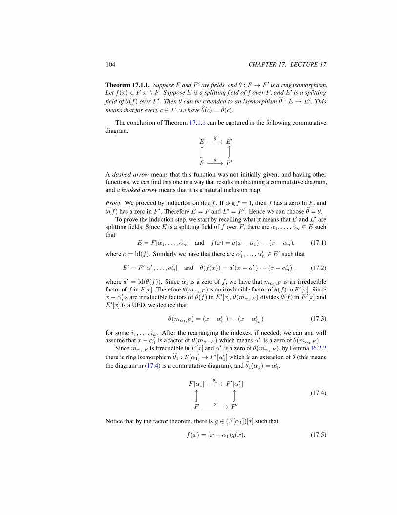
104 CHAPTER 17. LECTURE 17
Theorem 17.1.1. Suppose F and F ′ are fields, and θ : F → F ′ is a ring isomorphism.Let f(x) ∈ F [x] \ F . Suppose E is a splitting field of f over F , and E′ is a splittingfield of θ(f) over F ′. Then θ can be extended to an isomorphism θ : E → E′. Thismeans that for every c ∈ F , we have θ(c) = θ(c).
The conclusion of Theorem 17.1.1 can be captured in the following commutativediagram.
E E′
F F ′
θ
θ
A dashed arrow means that this function was not initially given, and having otherfunctions, we can find this one in a way that results in obtaining a commutative diagram,and a hooked arrow means that it is a natural inclusion map.
Proof. We proceed by induction on deg f . If deg f = 1, then f has a zero in F , andθ(f) has a zero in F ′. Therefore E = F and E′ = F ′. Hence we can choose θ = θ.
To prove the induction step, we start by recalling what it means that E and E′ aresplitting fields. Since E is a splitting field of f over F , there are α1, . . . , αn ∈ E suchthat
E = F [α1, . . . , αn] and f(x) = a(x− α1) · · · (x− αn), (17.1)
where a = ld(f). Similarly we have that there are α′1, . . . , α′n ∈ E′ such that
E′ = F ′[α′1, . . . , α′n] and θ(f(x)) = a′(x− α′1) · · · (x− α′n), (17.2)
where a′ = ld(θ(f)). Since α1 is a zero of f , we have that mα1,F is an irreduciblefactor of f in F [x]. Therefore θ(mα1,F ) is an irreducible factor of θ(f) in F ′[x]. Sincex− α′i’s are irreducible factors of θ(f) in E′[x], θ(mα1,F ) divides θ(f) in E′[x] andE′[x] is a UFD, we deduce that
θ(mα1,F ) = (x− α′i1) · · · (x− α′ik) (17.3)
for some i1, . . . , ik. After the rearranging the indexes, if needed, we can and willassume that x− α′1 is a factor of θ(mα1,F ) which means α′1 is a zero of θ(mα1,F ).
Sincemα1,F is irreducible in F [x] and α′1 is a zero of θ(mα1,F ), by Lemma 16.2.2there is ring isomorphism θ1 : F [α1]→ F ′[α′1] which is an extension of θ (this meansthe diagram in (17.4) is a commutative diagram), and θ1(α1) = α′1.
F [α1] F ′[α′1]
F F ′
θ1
θ
(17.4)
Notice that by the factor theorem, there is g ∈ (F [α1])[x] such that
f(x) = (x− α1)g(x). (17.5)

17.1. EXTENSION OF ISOMORPHISMS TO SPLITTING FIELDS. 105
By (17.5) and (17.1), we deduce that
g(x) = a(x− α2) · · · (x− αn). (17.6)
Applying θ1 to the both sides of (17.5), we obtain that
θ1(f) = (x− θ1(α1))θ1(g). (17.7)
Since θ1(α1) = α′1, by (17.2), it follows that
θ1(g) = a′(x− α′2) · · · (x− α′n). (17.8)
By (17.6), after adding zeros of g to F [α1]
(F [α1])[α2, . . . , αn] = F [α1, . . . , αn]
we getE. HenceE is a splitting field of g over F [α1]. Similarly, by (17.8), after addingzeros of θ1(g) to F ′[α′1] we getE′. ThereforeE′ is a splitting field of θ1(g) over F ′[α′1].Since deg g < deg f , we can and will apply the induction hypothesis. By the inductionhypothesis, we obtain a ring isomorphism θ : E → E′ which is an extension of θ1 (seethe commutative diagram given in (17.9)).
E E′
F [α1] F ′[α′1]
θ
θ1
(17.9)
By (17.4) and (17.9) (see the diagram in (17.10)),
E E′
F [α1] F ′[α′1]
F F ′
θ
θ1
θ
(17.10)
we deduce that θ is an extension of θ, which completes the proof.
The idea of the above proof is easy:
1. Find an irreducible factor of f in F [x], say h(x).
2. Add a zero of h to F and a zero of θ(h) to F ′, and find θ1 : F [α1]→ F ′[α′1].
3. View E as a splitting field of g and E′ as a splitting field of θ1(g). Use inductionhypothesis.

106 CHAPTER 17. LECTURE 17
Based on Theorem 17.1.1, we can prove the uniqueness of splitting fields up to anisomorphism.
Theorem 17.1.2. Suppose F is a field, f(x) ∈ F [x] \F , and E,E′ are splitting fieldsof f(x) over F . Then there is a ring isomorphism θ : E → E′ such that θ|F = idF ;that means for every c ∈ F we have that θ(c) = c.
Proof. Notice that idF : F → F is an isomorphism, and so by Theorem 17.1.1, thereis a ring isomorphism θ : E → E′ which is an extension of idF . This completes theproof.
17.2 Two examples
In general giving a precise description of a splitting field of a polynomial is a veryhard task. In this section, we learn two examples where to some extend we can describea splitting of the given polynomial.
Example 17.2.1. Let ζn := e2πi/n. Then Q[ζn] is a splitting field of xn − 1 over Q.
Proof. Notice that the multiplicative order of ζn is n. Hence (ζjn)n = 1 for everyinteger j in [0, n), and 1, ζn, . . . , ζ
n−1n are distinct. Therefore these are distinct zeros
of xn − 1. Thus by the generalized factor theorem, comparing the degrees and theleading coefficients, we obtain that
xn − 1 = (x− 1)(x− ζn) · · · (x− ζn−1n ).
Hence E := Q[1, ζn, . . . , ζn−1n ] is a splitting field of xn − 1 over Q. Notice that
Q[ζn] ⊆ E. Since ζjn ∈ Q[ζn] for every integer j, we have that E ⊆ Q[ζn]. The claimfollows.
Example 17.2.2. Let ζn := e2πi/n. Then Q[ζn,n√
2] is a splitting field of xn − 2 overQ.
Proof. Notice that (ζjnn√
2)n = 2 for every integer j. Hence n√
2, ζnn√
2, . . . , ζn−1n
n√
2are distinct zeros of xn − 2. Therefore by the generalized factor theorem, comparingdegrees and leading coefficients, we obtain that
xn − 2 = (x− n√
2)(x− ζn n√
2) · · · (x− ζn n√
2n−1
).
Therefore E := Q[ n√
2, ζnn√
2, . . . , ζn−1n
n√
2] is a splitting field of xn − 2 over Q.Notice that ζn := (ζn
n√
2)( n√
2)−1 ∈ E. Hence Q[ n√
2, ζn] ⊆ E. We also have thatζjn
n√
2 ∈ Q[ζn,n√
2] for every integer j. This implies that E ⊆ Q[ n√
2, ζn], and theclaim follows.
Next we use splitting fields to study finite fields.
Chapter 18
Lecture 18
In the previous couple of lectures we proved the following results about splittingfields.
Theorem (Existence (See Proposition 16.1.1)). Suppose F is a field and f ∈ F [x] \F .Then there is a s splitting field E of f over F .
Let’s recall that E is called a splitting field of f over F if there are α1, . . . , αn ∈ Esuch that f(x) = a(x− α1) · · · (x− αn), for some a ∈ F , and E = F [α1, . . . , αn].
Theorem (Uniqueness (See Theorem 17.1.2)). Suppose F is a field and f ∈ F [x] \ F ,E,E′ are splitting fields of f over F . Then there is θ : E → E′ such that for everyc ∈ F , θ(c) = c.
For field extensions E and E′ of F , we say a ring isomorphism θ : E → E′ is anF -isomorphism if θ(c) = c for every c ∈ F .
The Uniqueness result was proved using the following isomorphism extensiontheorem.
Theorem (Isomorphism extension (See Theorem 17.1.1)). Suppose F and F ′ are fields,θ : F → F ′ is an isomorphism, and f(x) ∈ F [x] \ F . Suppose E is a splitting fieldof f over F , and E′ is a splitting field of θ(f) over F ′. Then there is an isomorphismθ : E → E′ which is an extension of θ.
Prove of Isomorphism Extension Theorem is based on the following result onsending a zero of an irreducible polynomial to another zero.
Theorem (Sending a zero to another (See Lemma 16.2.2)). Suppose F and F ′ arefields, f is irreducible in F [x]. Suppose E is a field extension of which contains a zeroα of f , and E′ is a field extension of F ′ which contains a zero of θ(f). Then there isθ : F [α]→ F ′[α′] which is an extension of θ and θ(α) = α′.
Now we use these results to study finite fields.
107
108 CHAPTER 18. LECTURE 18
18.1 Finite fields: uniqueness
Suppose F is a finite field. Then its characteristic is a prime number p.
Lemma 18.1.1 (Order of a finite field). Suppose F is a finite of characteristic p. Then|F | = pn for some positive integer n.
Proof. Since F is a finite integral domain, p is prime. Suppose ` is a prime factor of|F |. Then by Cauchy’s theorem from group theory, there is a ∈ F such that the additiveorder of a is `. Since char(F ) = p, pa = 0. This implies that the additive order ` of adivides p. As ` and p primes, we deduce that ` = p. Hence the only prime factor of|F | is p, which implies that |F | is a power of p. This completes the proof.
We have seen that xp − x =∏a∈Zp(x− a). Next we generalize this to any finite
field. We start with the following lemma, which can be viewed as a generalization ofFermat’s little theorem.
Lemma 18.1.2. Suppose F is a finite field of order q. Then aq = a for every a ∈ F .
Proof. If a = 0, then clearly we have that aq = a. If a 6= 0, then a is a unit. Hencea|F
×| = 1 as we know that in every (multiplicative) group G we have g|G| = e. SinceF is a field, we have |F×| = |F | − 1 = q− 1. Therefore aq−1 = 1, which implies thataq = a. This completes the proof.
Theorem 18.1.3. Suppose F is finite field of order q. Then
xq − x =∏α∈F
(x− α)
in F [x].
Proof. By Lemma 18.1.2, every α ∈ F is a zero of xq − x. Hence by the generalizedfactor theorem, there is g(x) ∈ F [x] such that
xq − x = g(x)∏α∈F
(x− α). (18.1)
Comparing the degrees of both sides, we deduce that g is a non-zero constant. Sub-sequently comparing the leading coefficients of both sides of (18.1), we obtain thatg = 1. The claim follows.
Theorem 18.1.4 (Uniqueness). Suppose F is a finite field of order q = pn where p isa prime number. Then F is a splitting field of xq − x over Zp. In particular, if F andF ′ are two fields of order q, then they are isomorphic.
Proof. By Lemma 18.1.1, we obtain that the characteristic of F is p. Hence Zp can beviewed as a subfield of F . By Theorem 18.1.3, we have that xq − x can be factored asa product of degree one polynomials over F , and adding zeros of xq − x to Zp, we getthe entire F . Hence F is a splitting field of xq − x over Zp.
If F and F ′ are fields of order q, then both of them are splitting fields of xq − xover Zp. Hence by Theorem 17.1.2, F and F ′ are isomorphic. This completes theproof.

18.2. FINITE FIELDS: TOWARDS EXISTENCE 109
18.2 Finite fields: towards existence
We want to show the existence of a finite field of order q = pn where p is primeand n is a positive integer. By Theorem 18.1.4, we have to consider a splitting field Eof xq − x over Zp and show that it has q elements. So in this section, we let E be asplitting field of xq − x over Zp and
F := {α ∈ E | αq = α}.
Lemma 18.2.1. In the above setting, F is a field.
Proof. To show F is a field, we prove that is closed under addition, multiplication,negation, and inversion.
Notice that since the characteristic of F is a prime number p, the Frobenius mapσ : E → E, σ(a) := ap is a ring homomorphism (see Problem 4 in Week 1 assignment).Therefore
σ(n) : E → E, σ(n)(a) = apn
is also a ring homomorphism. Notice that F is the set of fixed points of σ(n); thatmeans that
F = {a ∈ E | σ(n)(a) = a}.For every α, β ∈ F , we have
σ(n)(α+β) = σ(n)(α)+σ(n)(β) = α+β and σ(n)(α·β) = σ(n)(α)·σ(n)(β) = α·β.
So α+ β and α · β are in F . Therefore F is closed under addition and multiplication.For α ∈ F we also have that
σ(n)(−α) = −σ(n)(α) = −α,
and so −α ∈ F . Suppose α ∈ F \ {0}. Then α−1 ∈ E, and
σ(n)(α−1) = (α−1)q = (αq)−1 = α−1,
which implies that α−1 ∈ F . This completes the proof.
Next we want to show that |F | = q, which completes the proof of the existence of afield of order q.
Corollary 18.2.2. In the above setting, the order of F is the same of the number ofdistinct zeros of xq − x in E.
Proof. Since E is a splitting field of xq − x over Zp, there are α1, . . . , αq ∈ E suchthat
xq − x =
q∏i=1
(x− αi).
Notice that α ∈ F if and only if α is a zero of xq − x. Since E is an integral domain,we obtain that
F = {α1, . . . , αn}.The claim follows.
110 CHAPTER 18. LECTURE 18
By Corollary 18.2.2, we have that |F | = q if and only if zeros of xq − x in itssplitting field are distinct. So we need to find a mechanism to determine whether zerosof a polynomial in its splitting field are distinct.
18.3 Separability: having distinct zeros in a splitting field.
We need to come up with a technique of finding out whether or not f(x) has amultiple zero. Recall that we say a ∈ A is a multiple zero of f if f(x) = (x− a)2g(x)for some g(x) ∈ A[x]. We use an idea from calculus: a polynomial f(x) ∈ C[x] has amultiple zero at z if and only if f(z) = f ′(z) = 0. This means we need to define thederivative of a polynomial in A[x] for an arbitrary unital commutative ring A.
Definition 18.3.1. Suppose f(x) :=∑∞i=0 aix
i ∈ A[x] where A is a unital commuta-tive ring. We let
f ′(x) :=
∞∑i=1
iaixi−1, (18.2)
and call it the derivative of f .
Sometimes it is useful to write the sum in (18.2) starting from 0
f ′(x) =
∞∑i=0
iaixi−1.
One can check that the following properties of ordinary derivatives still hold forpolynomials in a general setting.
Lemma 18.3.2. Suppose A is a unital commutative ring, f, g ∈ A[x], and a, b ∈ A.Then the derivative of af(x) + bg(x) is af ′(x) + bg′(x) and the product rule
(fg)′ = f ′g + fg′
holds.
Proof. It is easy to check that (af+bg)′ = af ′+bg′. Here we only discuss the productrule. Suppose f(x) =
∑∞i=0 aix
i and g(x) =∑∞j=0 bjx
j . Then the coefficient of xkin fg is
ck :=∑
i+j=k,i,j≥0
aibj .
Thus (fg)′ =∑∞k=0 kckx
k−1. Since f ′(x) =∑∞i=0 iaix
i−1 and g′(x) =∑∞j=0 jbjx
j−1,
the coefficient of xk−1 in f ′g is ∑i+j=k,i,j≥0
iaibj
and the coefficient of xk−1 in fg′ is ∑i+j=k,i,j≥0
jajbj .

18.3. SEPARABILITY: HAVING DISTINCT ZEROS IN A SPLITTING FIELD. 111
Hence
f ′g + fg′ =
∞∑k=0
( ∑i+j=k,i,j≥0
(i+ j)aibj
)xk−1 =
∞∑k=0
kckxk−1.
The claim follows.
Lemma 18.3.3. SupposeA is a unital commutative ring and for a ∈ A and f, g ∈ A[x],we have f(x) = (x− a)2g(x). Then f(a) = f ′(a) = 0.
Proof. Clearly f(a) = 0. By the product rule, we have that
f ′(x) = (x− a)2g(x) + 2(x− a)g(x) = (x− a)((x− a)g′(x) + 2g(x)).
Hence f ′(a) = 0. The claim follows.
Proposition 18.3.4. Suppose F is a field, f(x) ∈ F [x] \ F , and E is a splitting fieldof f over F . Then f(x) does not have multiple zeros in E if and only if gcd(f, f ′) = 1in F [x]1.
Proof. (⇒) Suppose gcd(f, f ′) 6= 1. Then there is a non-constant monic polynomialq(x) ∈ F [x] which divides both f(x) and f ′(x). Since E is a splitting field of f overF , there are α1, . . . , αn ∈ E such that
f(x) = a(x− α1) · · · (x− αn),
for some a ∈ F . As q(x)|f(x), x− αi’s are irreducible in E[x], and E[x] is a UFD,we have that
q(x) = (x− αi1) · · · (x− αik)
for some i1, . . . , ik. Since q(x)|f ′(x), we have that f ′(αi1) = 0. After rearranging theindexes, if necessary, we can and will assume that i1 = 1. Thus f ′(α1) = 0. By theproduct rule, we have that f ′(x) is equal to
a((x−α2) · · · (x−αn)+(x−α1)(x−α3) · · · (x−αn)+· · ·+(x−α1) · · · (x−αn−1)).
Hencef ′(α1) = a(α1 − α2) · · · (α1 − αn).
Therefore f ′(α1) = 0 implies that α1 = αj for some index j ≥ 2. This means f hasmultiple zeros.
(⇐) Suppose f(x) = (x − α)2g(x). Then by Lemma 18.3.3, f ′(α) = 0. Asf ′(x) ∈ F [x], we deduce that mα,F (x)|f ′(x) in F [x]. Similarly, since f(α) = 0 andf(x) ∈ F [x], we have mα,F (x)|f(x). Therefore mα,F (x) is a common divisor of fand f ′ in F [x], which implies that gcd(f, f ′) 6= 1. This completes the proof.
1Here we are using the convention that the greatest common divisor of polynomials with coefficients ina field are monic.

112 CHAPTER 18. LECTURE 18
18.4 Finite field: existence
Let’s recall some of the notation and results from Section 18.2. Let q = pn where pis a prime and n is a positive integer. Let E be a splitting field of xq − x over Zp. Let
F := {α ∈ E | αq = α}.
By Lemma 18.2.1, F is a field, and by Corollary 18.2.2, the order of F is the numberof distinct zeros of xq − x in E.
Lemma 18.4.1. In the above setting, |F | = q.
Proof. Since |F | is the number of distinct zeros of xq − x in its splitting field, it isenough to show that xq − x does not have multiple zeros in its splitting fields. ByProposition 18.3.4, f(x) := xq − x does not have multiple zeros in E if and only ifgcd(f, f ′) = 1 in F [x]. Notice that f ′(x) = qxq−1−1 = −1 in F [x] as char(F ) = p.Hence gcd(f, f ′) = 1, and the claim follows.
Altogether, we have proved:
Theorem 18.4.2 (Existence). Suppose p is prime and n is positive integer. Then thereis a finite field of order pn.
Theorem 18.4.3 (Construction). Finite field of order pn is a splitting field of xpn − x
over Zp.
We let Fpn denote a finite field of order pn. Notice that by Theorem 18.4.2, there issuch a finite field, and by Theorem 18.1.4, Fpn is unique up to an isomorphism.

Chapter 19
Lecture 19
19.1 Vector spaces over a field
Let’s recall a couple of results that we have proved a while ago.
Proposition. (See Proposition 8.3.1) Suppose F is a field and f(x) ∈ F [x] is apolynomial of degree n. Then every element of F [x]/〈f〉 can be uniquely written as
c01 + c1x+ · · ·+ cn−1xn−1
for some c0, . . . , cn−1 ∈ F where 1 := 1 + 〈f〉 and x := x+ 〈f〉.
Proposition. (See Theorem 9.1.1) Suppose E is a field extension oof F , and α ∈ E isalgebraic over F . Suppose degmα,F = n. Then every element of F [α] can be uniquelywritten as
c0 + c1α+ · · ·+ cn−1αn−1
for some c0, · · · , cn−1 ∈ F .
In both of these statements, elements are uniquely written as an F -linear combi-nation of certain elements. This is similar to the main property of a basis in a vectorspace. It brings us to the definition of a vector space over a field F .
Definition 19.1.1. Suppose F is a field. We say V is a vector space over F if:
(1) (V,+) is an abelian group.
(2) There is a scalar multiplication F × V → V and for every c ∈ F and v ∈ V ,the scalar multiplication of c by v is denoted by c · v (or simply cv). This scalarmultiplication is supposed to have the following properties.
a) For every c1, c2 ∈ F and v ∈ V ,
(c1 + c2) · v = c1 · v + c2 · v.
b) For every c ∈ F and v1, v2 ∈ V ,
c · (v1 + v2) = c · v1 + c · v2.
113

114 CHAPTER 19. LECTURE 19
c) For every v ∈ V , 1 · v = v.
Example 19.1.2. Suppose F is a field and n is a positive integer. Then
Fn := F × · · · × F︸ ︷︷ ︸n times
is a vector space with respect to the following scalar multiplication
c · (a1, . . . , an) := (ca1, . . . , can).
Another example which plays an important role in this course is the following.
Example 19.1.3. Suppose A is a unital ring, F is a subfield of A, and 1A = 1F . ThenA is a vector space over F with respect to the following scalar multiplication:
∀c ∈ F, a ∈ A, c · a := ca
where ca is the multiplication in A.
Let’s recall some basic terminologies in linear algebra.
Definition 19.1.4. Suppose V is a vector space over a field F .
1. We say v1, · · · , vn ∈ V are F -linearly independent if, for c1, . . . , cn ∈ F ,
c1 · v1 + · · ·+ cnvn = 0 implies that c1 = · · · = cn = 0.
2. If v1, . . . , vn ∈ V are not F -linearly independent, we say they are F -linearlydependent.
3. We say {v1, . . . , vn} ⊆ V is an F -spanning set if every element of V can bewritten as an F -linear combination of v1, . . . , vn; that means for every v ∈ Vthere are c1, . . . , cn ∈ F such that
v = c1 · v1 + · · ·+ cn · vn.
When {v1, . . . , vn} is an F -spanning set, we say v1, . . . , vn span V .
4. We say (v1, . . . , vn) is an F -basis of V if v1, . . . , vn are F -linearly independentand {v1, . . . , vn} is an F -spanning set.
Though a basis is formally an ordered set, we sometimes refer to a set as a basis ifit is an F -spanning set and consists of F -linearly independent vectors.

19.2. SUBSPACE AND LINEAR MAP 115
19.2 Subspace and linear map
As always, when we learn a new math object, we should talk about its substructuresand the maps that preserves its structure.
Definition 19.2.1. Suppose V is vector space over a field F . We say W ⊆ V is asubspace of V if W is closed under addition and scalar multiplication.
Definition 19.2.2. Suppose V1 and V2 are two vector spaces over a field F .
1. We say f : V1 → V2 is F -linear if
f(v + v′) = f(v) + f(v′) and f(c · v) = c · f(v)
for every c ∈ F and v, v′ ∈ V ; alternatively we can write f(cv + v′) =cf(v) + f(v′).
2. We say f : V1 → V2 is an isomorphism of F -vector spaces if
a) f is F -linear,b) f is bijective, andc) f−1 is F -linear.
It is a good exercise to show that if f is F -linear and it is bijective, then f−1 isF -linear. So the last condition for being an F -vector space isomorphism is redundant.
Let’s also point out that similar to Lemma 1.3.1, one can use the distributionproperties and show that
0F · v = 0V and c · 0V = 0V
for every v ∈ V and c ∈ F .
Lemma 19.2.3. Suppose V is a vector space over a field F , and v1, . . . , vn ∈ V . Thenthe smallest subspace of V which contains vi’s is{ n∑
i=1
civi | ci ∈ F}.
(This is denoted by SpanF {v1, . . . , vn} or SpanF (v1, . . . , vn), and it is called eitherthe F -span of vi’s, or the subspace spanned by v1, . . . , vn).
Proof. Suppose W is a subspace of V which contains vi’s. Since W is closed underscalar multiplication, we have civi ∈ W for every ci ∈ F . Since W is closed underaddition, we deduce that
∑ni=1 civi ∈W . Hence SpanF (v1, . . . , vn) ⊆W .
Next we show that Span(v1, . . . , vn) is a subspace. Suppose c ∈ F and w,w′ arein SpanF (v1, . . . , vn). Then w =
∑ni=1 civi and w′ =
∑ni=1 c
′ivi for some ci, c′i ∈ F .
Hence
cw + w′ = c
n∑i=1
civi +
n∑i=1
c′ivi =
n∑i=1
(cci + c′i)vi ∈ SpanF (v1, . . . , vn).

116 CHAPTER 19. LECTURE 19
Therefore SpanF (v1, . . . , vn) is a subspace.Finally we notice that
vi = 0 · v1 + · · ·+ 0 · vi−1 + 1 · vi + 0 · vi+1 + · · ·+ 0 · vn ∈ SpanF (v1, . . . , vn).
Altogether, we proved that SpanF (v1, . . . , vn) is a subspace which contains vi’s andevery other subspace that contains vi’ contains SpanF (v1, . . . , vn) as a subset. Thiscompletes the proof.
Next lemma shows the importance of Example 19.1.2.
Lemma 19.2.4. Suppose V is a vector space over a field F , and B := (v1, . . . , vn) isan F -basis of V . Then
1. for every v ∈ V , there is a unique
(c1, . . . , cn) ∈ Fn
such that v = c1v1 + · · ·+ cnvn. We let [v]B := (c1, . . . , cn).
2. The map V → Fn, v 7→ [v]B is a vector space isomorphism.
Proof. (1) Since B spans V , every v ∈ V can be written as an F -linear combinationof vi’s; that means that there are ci’s in F such that
v = c1v1 + · · ·+ cnvn.
Now we want to show the uniqueness. So suppose∑ni=1 civi =
∑ni=1 c
′ivi for some
ci, c′i ∈ F . Then
(c1 − c′1)v1 + · · ·+ (cn − c′n)vn = 0. (19.1)
As vi’s are F -linearly independent and ci − c′i ∈ F , by (19.1) we have that ci − c′i = 0for every i. Hence
(c1, . . . , cn) = (c′1, . . . , c′n).
(2) By part (1), v 7→ [v]B is well-defined and it is the inverse function of
Fn → V, (c1, . . . , cn) 7→n∑i=1
civi.
Hence v 7→ [v]B is a bijection. Let [v]B = (a1, . . . , an) and [v′]B = (a′1, . . . , a′n).
Then v =∑ni=1 aivi and v′ =
∑ni=1 a
′ivi. Therefore for every c, c′ ∈ F , we have
cv + cv′ =∑ni=1(cai + a′a′i)vi, which implies that
[cv + cv′]B =(ca1 + c′a′1, . . . , can + c′a′n)
=c(a1, . . . , an) + c′(a′1, . . . , a′n)
=c[v]B + c′[v′]B,
this completes the proof.

19.3. DIMENSION OF A VECTOR SPACE 117
19.3 Dimension of a vector space
The following theorem plays helps us define the dimension of a vector space andmore.
Theorem 19.3.1. Suppose V is a vector space over a field F . Suppose {v1, . . . , vn}is an F -spanning set, and w1, . . . , wm are F -linearly independent. Then n ≥ m.
Proof. Inductively we will find distinct indexes i1, . . . , im such that for every integer kin [0,m],
({v1, . . . , vn} \ {vi1 , . . . , vik}) ∪ {w1, . . . , wk}
is an F -spanning set. We are substituting wj for vij in {v1, . . . , vn} and still spanningV .
Notice that finding these distinct indexes
1 ≤ i1, . . . , im ≤ n
implies that m ≤ n, and the claim follows.The base of induction (k = 0) follows from the assumption that {v1, . . . , vn} is
an F -spanning set. Now we show the induction step. Suppose we have already foundi1, . . . , ik such that
({v1, . . . , vn} \ {vi1 , . . . , vik}) ∪ {w1, . . . , wk}
is an F -spanning set. To simplify our notation, after rearranging vi’s, we can and willassume that i1 = 1, . . . , ik = k; and so
SpanF (w1, . . . , wk, vk+1, . . . , vn) = V. (19.2)
In particular,wk+1 can be written as anF -linear combination ofw1, . . . , wk, vk+1, . . . , vn.Hence there are ci’s in F such that
wk+1 = c1w1 + · · ·+ ckwk + ck+1vk+1 + · · ·+ cnvn. (19.3)
Claim. There exists j ≥ k + 1 such that cj 6= 0.Proof of Claim. If not, wk+1 =
∑ki=1 ciwi. This contradicts the assumption that wi’s
are F -linearly independent.Without loss of generality, after rearranging vl’s, we can and will assume that
ck+1 6= 0.
Claim. SpanF (w1, . . . , wk+1, vk+2, . . . , vn) = V .Proof of Claim. Because of (19.2), to show the Claim it is sufficient to prove that vk+1
is in the F -span of w1, . . . , wk+1, vk+2, . . . , vn. By (19.3),
ck+1vk+1 = −k∑i=1
ciwi + wk+1 −n∑
i=k+2
civi.
118 CHAPTER 19. LECTURE 19
Notice that since ck+1 6= 0 and F is a field, c−1k+1 exists. Hence
vk+1 =−k∑i=1
(c−1k+1ci)wi + c−1
k+1wk+1 −n∑
i=k+2
(c−1k+1ci)vi
∈SpanF (w1, . . . , wk+1, vk+2, . . . , vn),
and the claim follows.
Theorem 19.3.2. Suppose V is a vector space over a field F . Suppose V is the F -spanof a finite set {v1, . . . , vn}. Then
1. V has an F -basis which is a subset of {v1, . . . , vn}.
2. If B := (w1, . . . , wm) and B′ := (w′1, . . . , w′k) are two F -bases, then m = k.
The size of a basis of V is called the dimension of V over F and we denote it bydimF V .
Proof of Theorem 19.3.2. (1) Suppose {vi1 , . . . , vim} is a maximal subset of {v1, . . . , vn}that consists of F -linearly independent vectors. Then for every j 6∈ {i1, . . . , im}, thevectors vi1 , . . . , vim , vj are F -linearly dependent. This means there are c1, . . . , cm+1 ∈F that are not all zero and
c1vi1 + · · ·+ cmvim + cm+1vj = 0.
Since vi1 , . . . , vim are F -linearly independent, cm+1 6= 0. Hence c−1m+1 exists (as F is
a field). Therefore
vj =− (c−1m+1c1)vi1 − · · · − (c−1
m+1cm)vim
∈SpanF (vi1 , . . . , vim). (19.4)
Since (19.4) holds for every j not in {i1, . . . , im}, we deduce that
SpanF (vi1 , . . . , vim) = SpanF (v1, . . . , vn) = V.
Hence (vi1 , . . . , vim) is an F -basis as it consists of F -linearly independent vectors andit is an F -spanning set.
(2) Since {w1, . . . , wm} is an F -spanning set and w′1, . . . , w′k are F -linearly in-dependent, by Theorem 19.3.1 we have k ≤ m. Similarly, since {w′1, . . . , w′k} is anF -spanning set and w1, . . . , wm are F -linearly independent, by Theorem 19.3.1 wehave m ≤ k. Altogether we get m = k, and this completes the proof.
19.4 Quotient spaces
Similar to groups and rings, we want to define the quotient of a vector space.Suppose V is a vector space over a field F , and W is a subspace of V . Then inparticular W is a (normal) subgroup of V . Hence we can consider the abelian groupV/W .
19.4. QUOTIENT SPACES 119
Proposition 19.4.1. Suppose V is a vector space over a field F , and W is a subspaceof V . Then the following is a well-defined scalar multiplication
F × V/W → V/W, (c, v +W ) 7→ c · (v +W ) := cv +W.
Moreover V/W with its quotient abelian group structure and the above given scalarproduct is an F -vector space.
Proof. Let’s start with arguing why · is a well-defined operation. So assuming v1+W =v2 + W , we have to show that cv1 + W = cv2 + W for every c ∈ F . Notice thatv1+W = v2+W implies that v1−v2 ∈W . AsW is closed under scalar multiplication,we have that c(v1 − v2) ∈W for every c in F . Therefore cv1 − cv2 ∈W , from whichwe deduce that cv1 +W = cv2 +W . This shows that · is a well-defined operation.
Next, we check why V/W is an F -vector space. For every c ∈ F and v1, v2 ∈ V ,we have
c · ((v1 +W ) + (v2 +W )) =c · ((v1 + v2) +W )
=c(v1 + v2) +W
=(cv1 + cv2) +W
=(cv1 +W ) + (cv2 +W )
=c · (v1 +W ) + c · (v2 +W ).
Similarly we can check that
(c1 + c2) · (v +W ) = c1 · (v +W ) + c2 · (v +W )
for every c1, c2 ∈ F and v ∈ V .Finally we observe that
1 · (v +W ) = (1 v) +W = v +W
for every v ∈ V . This completes the proof.
Notice that the natural quotient map
pW : V → V/W, pW (v) := v +W
is F -linear and ker pW = W .Since by Lemma 19.2.4 an F -vector space of a given dimension is unique up to an
isomorphism, we want to understand the dimension of V/W .
Proposition 19.4.2. Suppose V is a vector space over F and W is a subspace of V .Then
dimF W + dimF V/W = dimF V ;
in particular if one of the sides is finite, then the other side is finite as well.

120 CHAPTER 19. LECTURE 19
Proof. First notice that if dimF V <∞, then there is a finiteF -spanning set {v1, . . . , vn}.Then by Theorem 19.3.1, every subset of W that consists of F -linearly independentvectors has cardinality at most n; in particular, dimF W <∞. We also observe that{v1 +W, . . . , vn + W} is an F -spanning subset of V/W , and so by the first part ofTheorem 19.3.2, we have dimF V/W <∞. Hence from this point on, we can and willassume that
dimF W = m <∞ and dimF V/W = k <∞.
Suppose (w1, . . . , wm) is an F -basis of W , and (v1 +W, . . . , vk +W ) is an F -basisof V/W . We show that (w1, . . . , wm, v1, · · · , vk) is an F -basis of V . We prove this intwo steps. First we show this is an F -spanning set, and second we show that it consistsof F -linearly independent vectors.
Step 1. SpanF (w1, . . . , wm, v1, · · · , vk) = V .Proof of Step 1. Let W ′ := SpanF (w1, . . . , wm, v1, · · · , vk). Then W ⊆ W ′ as
wi’s spanW and they are inW ′. HenceW ′/W is a subspace of V/W . Since vi+W ’sare in W ′/W and they span V/W , we deduce that W ′/W = V/W . Therefore by thecorrespondence theorem for the subgroups of a quotient group, we have that V = W ′.(We can avoid using the correspondence theorem and use the following argument: forevery v ∈ V , knowing that v+W ∈W ′/W , we can deduce that there is w′ ∈W suchthat v +W = w′ +W . This means v − w′ = w for some w ∈W ⊆W ′. Hence
v = w′ + w ∈W ′.
Altogether we proved that every element v of V is in W . Therefore V = W ′.)Step 2. w1, . . . , wm, v1, · · · , vk are F -linearly independent.Proof of Step 2. Suppose
m∑i=1
ciwi +
k∑j=1
cm+jvj = 0 (19.5)
for some ci’s in F . Then
pW
( m∑i=1
ciwi +
k∑j=1
cm+jvj
)= 0,
where pW : V → V/W, pW (v) := v + W is the natural quotient map. SinceW = ker pW , we obtain that
k∑j=1
cm+j · pW (vj) = 0,
and socm+1 · (v1 +W ) + · · ·+ cm+k · (vk +W ) = 0. (19.6)
As vj + W ’s are F -linearly independent, we deduce that cm+1 = · · · = cm+k = 0.Hence by (19.5), we obtain that
m∑i=1
ciwi = 0.

19.5. THE FIRST ISOMORPHISM THEOREM FOR VECTOR SPACES 121
Aswi’s are F -linearly independent, we have c1 = · · · = cm = 0. Altogether we deducethat all the coefficients in (19.6) are zero. This completes the proof of the second step.
By Steps 1 and 2, we obtain that
(w1, . . . , wm, v1, . . . , vk)
is an F -basis. Hence
dimF V = m+ k = dimF W + dimF V/W,
which completes the proof.
19.5 The first isomorphism theorem for vector spaces
Similar to groups and rings, next we prove the first isomorphism theorem. Then weuse this result to show the kernel-image theorem.
Theorem 19.5.1. Suppose V1 and V2 are two F -vector spaces, and f : V1 → V2 is anF -linear map. Then
1. Im(f) is a subspace of V2, and ker f is a subspace of V1.
2. f : V1/ ker f → Im f, f(v1 + ker f) := f(v1) is an isomorphism of F -vectorspaces.
3. dimF (ker f) + dimF (Im f) = dimF V1.
Proof. (1) Since f is an additive group homomorphism, Im f is a subgroup of V2 andker f is a subgroup of V1. So it is sufficient to prove that Im f and ker f are closedunder scalar multiplication. Suppose v2 ∈ Im f . Then v2 = f(v1) for some v1 ∈ V1.Hence for every c ∈ F , we have
cv2 = cf(v1) = f(cv1) ∈ Im f.
This shows that Im f is closed under scalar multiplication, and so it is a subspace of V2.Suppose v1 ∈ ker f and c ∈ F . Then
f(cv1) = cf(v1) = c0 = 0,
which implies that cv1 ∈ ker f . Hence ker f is closed under scalar multiplication,which implies that ker f is a subspace of V1.
(2) By the first isomorphism theorem for groups, we have that
f : V1/ ker f → Im f, f(v1 + ker f) := f(v1)
is a well-defined group isomorphism. So to show that f is an F -vector space isomor-phism, it suffices to argue why f preserves the scalar multiplication. For every c ∈ F

122 CHAPTER 19. LECTURE 19
and v1 ∈ V1, we have
f(c · (v1 + ker f)) =f(cv1 + ker f)
=f(cv1)
=cf(v1)
=c · f(v1 + ker f),
and part (2) follows.(3) By Proposition 19.4.2 and the second part, we have
dimF (Im f) = dimF (V1/ ker f) = dimF V1 − dimF (ker f),
and the claim follows.

Chapter 20
Lecture 20
We have proved basic properties of vector spaces over a field F . Here we willexplore their implications in field theory.
20.1 Previous results in the language of linear algebra
We have motivated our digression to vector spaces over fields by considering theconclusions of Proposition 8.3.1 and Theorem 9.1.1. Here we rephrase those conclusionsusing terminologies from linear algebra.
Proposition 20.1.1. Suppose F is a field and f(x) ∈ F [x] is a polynomial of degree n,where n is a positive integer. Then (1, x, . . . , xn−1) is an F -basis of F [x]/〈f〉, wherexi := xi + 〈f〉 for every integer i in [0, n− 1]. In particular, dimF F [x]/〈f〉 = deg f .
Proof. By Proposition 8.3.1, every element of F [x]/〈f〉 can be uniquely written as
(c0 + c1x+ · · ·+ cn−1xn−1) + 〈f〉 =
n−1∑i=0
cixi.
Hence the F -span of {1, x, . . . , xn−1} is F [x]/〈f〉. Moreover if∑n−1i=0 cix
i = 0, thenbecause of the uniqueness the above expression we obtain that ci’s are 0. This impliesthat 1, x, . . . , xn−1 are F -linearly independent. The claim follows.
Proposition 20.1.2. Suppose E is a field extension of F , and α ∈ E is algebraic overF . Then (1, α, . . . , αn−1) is an F -basis of F [α] where n = degmα,F . In particular,dimF F [α] = degmα,F .
Proof. By Theorem 9.1.1, every element of F [α] can be uniquely written as
c0 + c1α+ · · ·+ cn−1αn−1
for some c0, . . . , cn−1 ∈ F wheren = degmα,F . Hence theF -span of {1, α, . . . , αn−1}is F [α]. Moreover if
∑n−1i=0 ciα
i = 0, then because of the uniqueness the above ex-pression we obtain that ci’s are 0. This implies that 1, α, . . . , αn−1 are F -linearlyindependent. The claim follows.
123

124 CHAPTER 20. LECTURE 20
20.2 Finite fields and vector spaces
Suppose F is a finite field and V is a vector space over F . If dimF V = n, then byLemma 19.2.4, we have that V ' Fn, and so
|V | = |F |dimF V . (20.1)
This helps us get a strong condition for the tower of finite fields.
Proposition 20.2.1. If Fpm can be embedded into Fpn , then m|n.
Proof. If Fpm can be embedded into Fpn , we can view Fpn as a vector space over Fpm .Since these are finite sets, dimFpm Fpn = d <∞. Hence by (20.1), we have
|Fpn | = |Fpm |d, which implies that n = md.
This completes the proof.
One can use the cardinality of the group of units of finite fields to prove the sameresult. Assuming that Fpm can be embedded in Fpn , we deduce that the group of unitsof Fpm can be embedded into the group of units of Fpn . Hence pm − 1|pn − 1. Fromthis one can show that m|n. As you can see the presented proof, which is based onlinear algebra, is much more natural.
Exercise 20.2.2. Suppose m and n are positive integers and m|n. Prove that Fpm canbe embedded into Fpn .
20.3 Tower rule for field extensions
We have already seen in Proposition 20.2.1 how useful it is to think about a fieldextension E of F as an F -vector space.
Definition 20.3.1. Suppose E is a field extension of F . Then we can view E as anF -vector space (see Example 19.1.3). The dimension dimF E of E as an F -vectorspace is denoted by [E : F ] and it is called the degree of this field extension.
Theorem 20.3.2 (Tower rule). Suppose L is a field extension of E,and E is a field extension of F . Then
[L : F ] = [L : E][E : F ];
in particular, if one of the sides is finite, then the other side is finite aswell.
L
E
F
(20.2)
We often use a diagram as in (20.2) to show field extensions. In this type of diagram,we connect two fields if one is a subfield of the other. The subfield is located lower thanthe larger field.

20.3. TOWER RULE FOR FIELD EXTENSIONS 125
Proof of Theorem 20.3.2. If [L : F ] = n < ∞, then there is a finite F -spanning set{v1, . . . , vn}. Hence the L-span of {v1, . . . , vn} is also L, and so by Theorem 19.3.2,[L : E] ≤ n. And also, by Proposition 19.4.2, we have
[E : F ] = dimF E ≤ dimF L <∞.
Therefore from this point on, we can and will assume that
[L : E] = m <∞ and [E : F ] = n <∞.
Suppose (`1, . . . , `m) is an E-basis of L, and (e1, . . . , en) is an F -basis of E. Weprove that
{`iej | 1 ≤ i ≤ m, 1 ≤ j ≤ n}(with respect to some ordering) is an F -basis of L. We do this in two steps.
Step 1. SpanF (`iej | 1 ≤ i ≤ m, 1 ≤ j ≤ n) = L.Proof of Step 1. Every ` ∈ L can be written as an E-linear combination of `i’s.
This means there are xi ∈ E such that
` = x1`1 + · · ·+ xm`m. (20.3)
Every element of E can be written as an F -linear combination of ej’s. Hence for everyi, there are yij ∈ F such that
xi = yi1e1 + · · ·+ yinen. (20.4)
By (20.3) and (20.4), we deduce that
` =
m∑i=1
xi`i =
m∑i=1
( n∑j=1
yijej
)`i
=∑
1≤i≤m,1≤j≤n
yij `iej .
This means ` can be written as an F -linear combination of `iej’s. This completes theproof of Step 1.
Step 2. `iej’s are F -linearly independent.Proof of Step 2. Suppose ∑
1≤i≤m,1≤j≤n
yij `iej = 0 (20.5)
for some yij’s in F . Then by (20.5), we havem∑i=1
( n∑j=1
yijej
)`i = 0. (20.6)
Notice that for every i, xi :=∑nj=1
∑nj=1 yijej is in E. Since `i’s are E-linearly
independent, by (20.6) we deduce that xi = 0 for every i. Hence we haven∑j=1
n∑j=1
yijej = 0 (20.7)

126 CHAPTER 20. LECTURE 20
for every index i. Since ej’s are F -linearly independent, by (20.7) we obtain thatyij = 0 for every pair of indexes i and j. This completes the proof of the second step.
By Steps 1 and 2, we deduce that
[L : F ] = |{`iej | 1 ≤ i ≤ m, 1 ≤ j ≤ n}| = mn = [L : E][E : F ],
which completes the proof.
20.4 Some applications of the Tower Rule for field extensions
Here we mention some examples on how one can use the Tower Rule.
Example 20.4.1. Suppose E is a field extension of Q such that [E : Q] = 2n for somepositive integer n. Then x3 − 2 is irreducible in E[x].
Proof. Suppose to the contrary that x3 − 2 is not irreducible in E[x].Then by the irreducibility criterion for degree 2 and 3 polynomials(see 10.1.1), we deduce that there is α ∈ E which is a zero of x3 − 2.Then Q[α] is an intermediate field; that means we have the towerof field extensions given in (20.9). Hence by the Tower Rule (seeTheorem 20.3.2), we have [E : Q] = [E : Q[α]][Q[α] : Q]. Thereforeby Proposition 20.1.2 and our hypothesis, we obtain that
2n = [E : Q[α]] degmα,Q. (20.8)
E
Q[α]
Q
(20.9)
So we it is useful to find the minimal polynomial mα,Q of α over Q. Notice that α is azero of x3 − 2, x3 − 2 is monic, and by Eisenstein’s irreducibility criterion (see Theo-rem 12.2.1), x3−2 is irreducible in Q[x]. Hence by Theorem 8.2.5,mα,Q(x) = x3−2.Thus by (20.8), 3 is a divisor of 2n which is a contradiction. This completes theproof.
Example 20.4.2. Suppose E is a field extension of F and α ∈ E is algebraic over F .Suppose [F [α] : F ] is odd. Then F [α] = F [α2].
Proof. Notice that F [α] is a field extension of F [α2].So we have the tower of field extensions given in (20.11). Henceby the Tower Rule (see Theorem 20.3.2), we have
[F [α] : F ] = [F [α] : F [α2]][F [α2] : F ].
Therefore by Proposition 20.1.2 and our hypothesis, we obtainthat
(degmα,F [α2])[F [α2] : F ] is odd. (20.10)
F [α]
F [α2]
F
(20.11)
By (20.10), we have that degmα,F [α2] is odd. Notice thatα is a zero of x2−α2 ∈ F [α2].Hence degmα,F [α2] ≤ 2. As the only positive odd integer less than or equal to 2 is 1,we have degmα,F [α2] = 1. This implies that α ∈ F [α2], and so F [α] ⊆ F [α2]. Theclaim follows.
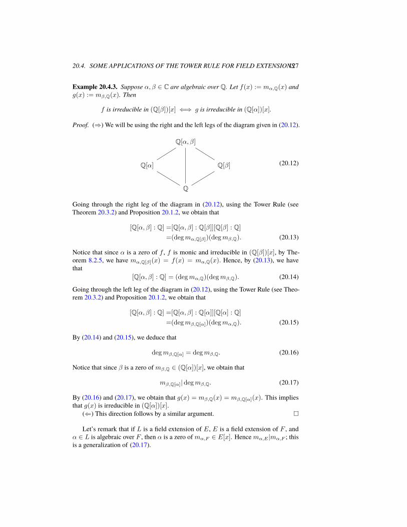
20.4. SOME APPLICATIONS OF THE TOWER RULE FOR FIELD EXTENSIONS127
Example 20.4.3. Suppose α, β ∈ C are algebraic over Q. Let f(x) := mα,Q(x) andg(x) := mβ,Q(x). Then
f is irreducible in (Q[β])[x] ⇐⇒ g is irreducible in (Q[α])[x].
Proof. (⇒) We will be using the right and the left legs of the diagram given in (20.12).
Q[α, β]
Q[α] Q[β]
Q
(20.12)
Going through the right leg of the diagram in (20.12), using the Tower Rule (seeTheorem 20.3.2) and Proposition 20.1.2, we obtain that
[Q[α, β] : Q] =[Q[α, β] : Q[β]][Q[β] : Q]
=(degmα,Q[β])(degmβ,Q). (20.13)
Notice that since α is a zero of f , f is monic and irreducible in (Q[β])[x], by The-orem 8.2.5, we have mα,Q[β](x) = f(x) = mα,Q(x). Hence, by (20.13), we havethat
[Q[α, β] : Q] = (degmα,Q)(degmβ,Q). (20.14)
Going through the left leg of the diagram in (20.12), using the Tower Rule (see Theo-rem 20.3.2) and Proposition 20.1.2, we obtain that
[Q[α, β] : Q] =[Q[α, β] : Q[α]][Q[α] : Q]
=(degmβ,Q[α])(degmα,Q). (20.15)
By (20.14) and (20.15), we deduce that
degmβ,Q[α] = degmβ,Q. (20.16)
Notice that since β is a zero of mβ,Q ∈ (Q[α])[x], we obtain that
mβ,Q[α]|degmβ,Q. (20.17)
By (20.16) and (20.17), we obtain that g(x) = mβ,Q(x) = mβ,Q[α](x). This impliesthat g(x) is irreducible in (Q[α])[x].
(⇐) This direction follows by a similar argument.
Let’s remark that if L is a field extension of E, E is a field extension of F , andα ∈ L is algebraic over F , then α is a zero of mα,F ∈ E[x]. Hence mα,E |mα,F ; thisis a generalization of (20.17).

128 CHAPTER 20. LECTURE 20
20.5 Algebraic closure in a field extension
Suppose E is a field extension of F . The algebraic closure of F in E is the set ofall the elements of E that are algebraic over F . Here we will prove that the algebraicclosure of F in E is a subfield of E. We start with proving that a field extension offinite degree is an algebraic extension.
Lemma 20.5.1. SupposeE is a field extension of F of finite degree. Then every α ∈ Eis algebraic over F .
We say a field extensionE of F is an algebraic extension if every α ∈ E is algebraic.So we are proving that a field extension of finite degree is algebraic.
Proof of Lemma 20.5.1. Suppose [E : F ] = n. Then by Theorem 19.3.1, every n+ 1elements of E are F -linearly dependent. Hence 1, α, . . . , αn are F -linearly dependent.Thus there are c0, . . . , cn ∈ F that are not all zero and
c0 + c1α+ · · ·+ cnαn = 0.
This means that α is algebraic over F .
Theorem 20.5.2 (Algebraic closure in a field extension). SupposeE is a field extensionof F . Let
K := {α ∈ E | α is algebraic over F}.
Then K is a field extension of F .
Proof. Suppose α, β ∈ K. Then by Proposition 20.1.2, we have [F [α] : F ] =degmα,F <∞. Moreover as β is algebraic over F [α], we have [F [α, β] : F [α]] <∞.Hence by the Tower Rule (see Theorem 20.3.2) we obtain that
[F [α, β] : F ] = [F [α, β] : F [α]][F [α] : F ] <∞. (20.18)
By Lemma 20.5.1 and (20.18), we deduce that F [α, β] is an algebraic extension of F ;this means that F [α, β] ⊆ K. This implies that F ⊆ K, α± β and αβ are in K, andif β 6= 0, then αβ−1 is in K, as well. Altogether, we deduce that K is field extensionof F . This completes the proof.
20.6 Tower of algebraic extensions
Here we show another application of the tower rule on algebraic extensions.
Proposition 20.6.1. Suppose E is an algebraic extension field of F and L is an alge-braic extension field of E. Then L is an algebraic extension field of F .
Proof. Suppose α ∈ L. Then α is algebraic over E. Suppose
mα,E(x) = xn + en−1xn−1 + · · ·+ e0

20.7. GEOMETRIC CONSTRUCTIONS BY RULER AND COMPASS 129
is the minimal polynomial of α over E. Hence α is algebraic over F [e0, . . . , en−1].Notice that since ei’s are algebraic over F , by the Tower rule by an argument similar to(20.18) inductively we can show that
[F [e0, . . . , en−1] : F ] <∞. (20.19)
As α is algebraic over F [e0, . . . , en−1],
[F [e0, . . . , en−1][α] : F [e0, . . . , en−1]] <∞. (20.20)
Hence by the Tower Rule, (20.19), and (20.20), we have
[F [e0, . . . , en−1, α] : F ] <∞.
Therefore by Lemma 20.5.1, α is algebraic over F . This completes the proof.
20.7 Geometric constructions by ruler and compass
Let’s recall some ancient Euclidean geometry problems. Can we construct 3√
2, π,or angle 20◦ using ruler and compass? Let’s formulate it properly what it means toconstruct a number. We start with a unit segment. The end points are consideredconstructed. If two points are constructed, then the line which passes through them isconsidered constructed. The circles that are centered at one of these points and passthrough the other are called constructed. The points of intersection of constructedcircles and lines are considered constructed points. A number is called constructedif its absolute value is the distance of two constructed points. The following theoremgives us an excellent understanding of constructed points.
Theorem 20.7.1. Suppose the initial points are (0, 0) and (1, 0). If (α, β) is a con-structed point, then [Q[α] : Q] and [Q[β] : Q] are powers of 2.
Here only the main ideas will be presented. To get to the point (α, β), we haveto construct finitely many lines and circles, and consider their intersection points. Tofind the coordinates of intersection points we end up solving degree 1 and degree 2polynomials with coefficients that are in the ring generated by the coordinates of theconstructed points that we have so far. This means there is a tower of field extensions
Q =: F0 ⊆ F1 ⊆ · · · ⊆ Fn
such that [Fi+1 : Fi] = 2 for every i and α ∈ Fn. By the Tower Rule, [Fn : Q] ispower of 2. Since Q[α] is an intermediate subfield, by the Tower Rule we deduce that[Q[α] : Q] divides [Fn : Q]. Hence [Q[α] : Q] is a power of 2.
Corollary 20.7.2. 3√
2 and π cannot be constructed by ruler and compass.
Proof. By Theorem 20.7.1, if α can be constructed by ruler and compass, then [Q[α] :Q] is a power of 2. In particular, α is algebraic. Hence π cannot be constructed (wedo not prove this here, but it can be proved that π is not algebraic over Q). Notice thatdegm 3√2,Q = 3, and so 3
√2 cannot be constructed by ruler and compass.

130 CHAPTER 20. LECTURE 20
Exercise 20.7.3. Show that degmcos 20◦,Q = 3, and use this to deduce the angle 20◦
cannot be constructed by ruler and compass. (Hint: cos 3θ = 4 cos3 θ − 3 cos θ.)
By the above Exercise, we can deduce that there is no general method of dividing agiven angle into three equal parts using only ruler and compass.
Chapter 21
Lecture 21
By now we have a basic understanding of vector spaces over a field and how it canhelp us study field extensions. We go back and further study splitting fields. Here wefocus on the splitting field of xn − 1 over Q. Let us recall that by Example 17.2.1, wehave that Q[ζn] is a splitting field of xn − 1 over Q, where ζn := e2πi/n, and
xn − 1 = (x− 1)(x− ζn) · · · (x− ζn−1n ). (21.1)
This field has a historical significance, because of its role in the initial modern attemptstowards proving Fermat’s last conjecture. We want to answer a very basic questionabout this field: what is [Q[ζn] : Q]? By Proposition 20.1.2, we have
[Q[ζn] : Q] = degmζn,Q.
Hence we need to find the minimal polynomial of ζn over Q.
21.1 Cyclotomic polynomials
In this section, we will arrive at the definition of the n-th cyclotomic polynomial.This will be done as we investigate the minimal polynomial of ζn over Q.
Notice that since ζn is a zero of xn − 1, mζn,Q divides xn − 1. Hence by (21.1)and the fact the C[x] is a UFD, we deduce that
mα,Q(x) = (x− ζi1n ) · · · (x− ζimn )
for some integers ij’s in [1, n]. As ζn is a zero of mζn,Q, without loss of generality, wecan and will assume that i1 = 1.
By Lemma 16.2.2, if E is a field extension of F and α, α′ ∈ E are two zeros ofan irreducible polynomial f ∈ F [x], then there is an F -isomorphism θ : F [α] →F [α′] such that θ(α) = α′; an F -isomorphism is a ring isomorphism which F -linear.Applying this result for the two zeros ζn and ζijn of the irreducible polynomialmζn,Q ∈Q[x], we obtain a Q-isomorphism θj : Q[ζn]→ Q[ζ
ijn ] such that θj(ζn) = ζ
ijn . Notice
that, since θj is a ring isomorphism, the multiplicative order of ζn and θj(ζn) are
131

132 CHAPTER 21. LECTURE 21
the same. As o(gk) = o(g)gcd(o(g),k) , o(ζn) = n, and θj(ζn) = ζ
ijn , we deduce that
gcd(n, ij) = 1 for every j. This takes us to the definition of the n-th cyclotomicpolynomial.
Definition 21.1.1. The n-th cyclotomic polynomial is
Φn(x) :=∏
1≤i≤n,gcd(i,n)=1
(x− ζin).
In particular, Φn is a monic polynomial of degree φ(n), wherer φ is the Euler-phifunction.
By the above discussion, we have that mζn,Q(x) divides Φn(x) in C[x]. We willprove that mζn,Q(x) = Φn(x).
21.2 Cyclotomic polynomials are integer polynomials
The following is a key property of cyclotomic polynomials that, among other things,help us prove cyclotomic polynomials are integer polynomials.
Theorem 21.2.1. For every positive integer n, we have
xn − 1 =∏d|n
Φd(x). (21.2)
Before we go to the details of the proof of Theorem 21.2.1, let us compare thedegrees of the both sides of (21.2):
n =∑d|n
φ(d). (21.3)
Proof of this formula is based on the partitioning of the set [1..n] := {1, . . . , n} interms of the greatest common divisor of the elements with n. To be more precise, welet
Cd,n := {i ∈ [1..n] | gcd(i, n) = d}. (21.4)Then {Cd,n | d|n} is a partitioning of [1..n]. Moreover
i ∈ Cd,n ⇐⇒ gcd(i, n) = d ⇐⇒ i = dj and gcd(j,n
d
)= 1.
Hence
Cd,n = {dj | j ∈ C1,nd} which imlies that |Cd,n| = |C1,nd
| = φ(nd
). (21.5)
Thereforen = |[1..n]| =
∑d|n
|Cd,n| =∑d|n
φ(nd
).
Finally we notice that as d ranges over all the positive divisors of n, so does nd ; that
means d 7→ nd is a bijection from the set of positive divisors of n to itself. Hence∑
d|n φ(nd ) =∑d|n φ(d), and (21.3) follows. We will be following the same steps to
prove (21.2).

21.2. CYCLOTOMIC POLYNOMIALS ARE INTEGER POLYNOMIALS 133
Proof of Theorem 21.2.1. Since xn − 1 =∏i∈[1..n](x − ζin) and {Cd,n | d|n} is a
partition of [1..n], we have that
xn − 1 =∏d|n
∏i∈Cd,n
(x− ζin). (21.6)
By (21.5), we have that ∏i∈Cd,n
(x− ζin) =∏
j∈C1, nd
(x− ζdjn ). (21.7)
Notice that ζdn = e(2πi/n)d = e2πi/(nd ) = ζnd
. So by (21.7), we deduce that∏i∈Cd,n
(x− ζin) =∏
0≤j<nd ,gcd(j,nd )=1
(x− ζjnd
) = Φnd
(x). (21.8)
By (21.6) and (21.8), we obtain
xn − 1 =∏d|n
Φnd
(x). (21.9)
As it is mentioned earlier, d 7→ nd is a bijection from the set of positive divisors of n to
itself. Hence by (21.9), (21.2) follows.
Using we are ready to prove that cyclotomic polynomials are integer polynomials.
Corollary 21.2.2. For every positive integer n, Φn(x) ∈ Z[x].
Proof. We proceed by strong induction on n. The base case is clear as Φ1(x) = x− 1.Next we prove the strong induction step. By the strong induction hypothesis, for everypositive integer m < n, Φm(x) ∈ Z[x]. Hence
Ψn(x) :=∏
d|n,d 6=n
Φd(x) ∈ Z[x], (21.10)
and as Φd’s are monic, Ψn(x) is monic as well. By Theorem 21.2.1, we have
xn − 1 = Φn(x)Ψn(x). (21.11)
As xn − 1,Ψn(x) ∈ Z[x] and Ψn(x) is monic, by the Long Division for elements inZ[x] (see Theorem 6.4.1) there are unique q(x), r(x) ∈ Z[x] such that
1. xn − 1 = q(x)Ψn(x) + r(x) and
2. deg r < deg Ψn.
Using the Long Division for elements in C[x], we see that the same q and r are thequotient and remainder of xn − 1 divided by Ψn(x) as elements of C[x]. By (21.11),however, we have that the quotient and the remainder of xn − 1 divided by Ψn(x) aselements of C[x] are Φn(x) and 0, respectively. Hence Φn(x) = q(x) ∈ Z[x], and theclaim follows.
134 CHAPTER 21. LECTURE 21
Let us remark that the last part of the above argument implies the following:
Lemma 21.2.3. Suppose A is a subring of a unital commutative ring B and 1B ∈ A.Suppose f, g ∈ A[x] and ld(f) ∈ A×. If f |g in B[x], then f |g in A[x].
Use long division in A[x] and B[x] to prove this Lemma. I leave it to you to fill outthe details.
21.3 Cyclotomic polynomials are irreducible
The main goal of this section is to prove the following:
Theorem 21.3.1. For every integer n, Φn(x) is irreducible in Q[x].
As before the general steps are proceeding by contradiction, going from Q to Z,and using the residue maps modulo primes. The last step, however, will be more subtlethan the other examples that we have done so far.
Proof of Theorem 21.3.1. Suppose to the contrary that Φn(x) is not irreducible in Q[x].Then Φn(x) = f(x)g(x) for some non-constant smaller degree polynomials f and g.Since Φn(x) is a monic integer polynomial, it is a primitive polynomial. By Gauss’slemma (see Corollary 15.4.3), we have Φn(x) = f(x)g(x) where f and g are primitiveforms of f and g, respectively. Notice that ζn is a zero Φn, it is either a zero of f ora zero of g. Without loss of generality, we can and will assume that ζn is a zero of f .Every other zero ζ of f is a zero of Φn(x), and so the multiplicative order of ζ (as anelement of C×) is n.
(Here is where the magic is happening.)If p is a prime which does not divide n and ζ ∈ C× has multiplicative order n, then
the multiplicative order of ζp is also n. Therefore ζp is a zero of Φn(x), and so it is azero of either f or g.
Claim 1. If ζ is a zero of f and p is a prime which does not divide n, then ζp is azero of f as well.
Proof of Claim 1. Suppose to the contrary that f(ζp) 6= 0. Since o(ζp) = n, Φn(ζp) =0. As f(ζp) 6= 0 and Φn(ζp) = f(ζp)g(ζp), we deduce that g(ζp) = 0. This meansζ is a common zero of f(x) and g(xp). Thus mζ,Q(x) is a common divisor of f(x)and g(xp) in Q[x]. Let h(x)Z[x] be the primitive form of mζ,Q(x). By Gauss’s lemma(see Corollary 15.4.3), h(x) is a common divisor of f(x) and g(xp) in Z[x]. As f ismonic, so is h. Therefore cp(h) is a common divisor of cp(f(x)) and cp(g(xp)) wherecp : Z[x]→ Zp[x] is the residue map modulo p. Notice that h is a monic non-constantpolynomial, so is cp(h).
(Here you see why we considered raising to power p at the first place.)Since Zp[x] is of characteristic p, by Fermat’s little theorem we have
cp(h(x))p = cp(h(xp)). (21.12)

21.4. THE DEGREE OF CYCLOTOMIC EXTENSIONS 135
To see this better, notice that in Zp[x] we have
(
∞∑i=0
aixi)p =
∞∑i=0
api (xi)p =
∞∑i=0
ai(xp)i.
So cp(h) is a non-constant common divisor of cp(f) and cp(g)p. Let `(x) be a primefactor of cp(h). Then `(x) divides cp(g)p, and so `(x) divides cp(g) as Zp[x] is a UFD.Therefore `(x)2 divides
cp(f)cp(g) = cp(fg) = cp(Φn). (21.13)
As cp(Φn) divides xn − 1 in Zp[x], `(x)2 divides xn − 1 in Zp[x]. Hence xn − 1has multiple zeros in its splitting field over Zp. By Proposition 18.3.4, we deducethat gcd(xn − 1, nxn−1) 6= 1. This is a contradiction as p - n and x - xn − 1. Thiscompletes the proof of Claim 1.
Claim 2. Suppose i is a positive integer and gcd(i, n) = 1. If ζ is a zero of f , thenζi is a zero of f .
Proof of Claim 2. We proceed by induction on the number k of prime factors of i.In the base case of k = 0, we have i = 1, and there is nothing to prove. Supposei = p1 · · · pk+1, where pj’s are primes that do not divide n. By the induction hypothesisζp1···pk is a zero of f . By Claim 1, we deduce that
(ζp1···pk)pk+1 = ζi
is a zero of f . This completes the proof of Claim 2.
By Claim 2, since ζn is a zero of f , ζin is a zero of f if i is a positive integerand gcd(i, n) = 1. This implies that Φn(x) divides f , which is a contradiction asdeg f < deg Φn. This completes the proof.
21.4 The degree of cyclotomic extensions
Field Q[ζn] is called a cyclotomic extension.
Theorem 21.4.1. Suppose n is a positive integer and ζn := e2πi/n. Then the minimalpolynomial of ζn over Q is mζn,Q(x) = Φn(x) and [Q[ζn] : Q] = φ(n).
Proof. We have that ζn is a zero of Φn(x), Φn(x) is a monic polynomial, and Φn(x)is irreducible in Q[x] (by Theorem 21.3.1). Hence by Theorem 8.2.5, we have thatmζn,Q(x) = Φn(x). By Proposition 20.1.2, we have
[Q[ζn] : Q] = degmζn,Q = deg Φn = φ(n),
which completes the proof.

Chapter 22
Lecture 22
22.1 The group of automorphism of a field extension.
Through out this course one of our main goals has been understanding zeros ofpolynomials. We proved the existence and the uniqueness (up to an isomorphism) ofa smallest field which contains all the zeros of a given polynomial (a splitting field).A better understanding of splitting fields can help us to learn more about the zeros ofpolynomials. One of our main tools of characterizing (intricate) objects is their group ofsymmetries. The group of symmetries of a field extension E of F is defined as follows.
Definition 22.1.1. For a field extension E of F , let
AutF (E) := {θ : E → E | θ is a ring isomorphism, and F -linear}.
An element of AutF (E) is called an F -automorphism. An F -linear, ring homomor-phism is called an F -homomorphism.
One can easily see that AutF (E) is a group under composition. We would like toknow how much AutF (E) tells us about the field extension.
Similar to the proof of the uniqueness of splitting fields, we need to work with two,possibly different, copies of the base field F , and with not necessarily surjective ringhomomorphisms: we proved the isomorphism extension theorem in order to deducethe uniqueness of splitting fields up to an isomorphism. That is why we introduce thefollowing notation.
Definition 22.1.2. Suppose θ : F → F ′ is a field isomorphism, E is a field extensionof F , and L′ is a field extension of F ′. Then
Embθ(E,L′) := {θ : E → L′ | θ injective ring homomorphism and θ|F = θ}
and an element of Embθ(E,L′) is called an θ-embedding. An isomorphism which is
an θ-embedding is called an θ-isomorphism, and the set of θ-isomorphisms is denotedby Isoθ(E,L
′). When F ′ = F and θ = idF , we write EmbF (E,L′) instead ofEmbidF (E,L′). Instead of saying idF -embedding, we say F -embedding.
137

138 CHAPTER 22. LECTURE 22
Notice that θ is in Embθ(E,L′) exactly when the following is a commutative
diagram.
E L′
F F ′
θ
θ
Lemma 22.1.3. If [E : F ] <∞, then EmbF (E,E) = AutF (E).
Proof. Clearly AutF (E) ⊆ EmbF (E,E). Suppose θ ∈ EmbF (E,E). To showthat θ is an F -automorphism, it suffices to argue why θ is surjective. By the firstisomorphism theorem for vector spaces (see Theorem 19.5.1), we have
dimF Im(θ) + dimF ker(θ) = dimF E.
Since θ is a injective, ker θ = 0. Hence dimF Im(θ) = dimF E. Since ImF (θ) is asubspace of E and it has the same dimension as E, by Proposition 19.4.2 Im(θ) = E.This completes the proof.
The following easy lemma is the corner stone of our understanding of the group ofsymmetries of algebraic field extensions.
Lemma 22.1.4. Suppose θ : F → F ′ is a field isomorphism, E is a field extension ofF , and L′ is a field extension of F ′. Suppose f(x) ∈ F [x] and α ∈ E is a zero of f .Then
for every θ ∈ Embθ(E,L′), θ(α) is a zero of θ(f).
In particular, if L is a field extension of F , then
for every F -embedding θ : E → L, θ(α) is a zero of f .
Proof. Suppose f(x) =∑ni=0 cix
i. Then∑ni=0 ciα
i = 0. Therefore
0 = θ( n∑i=0
ciαi)
=n∑i=0
θ(ci)θ(α)i =∑i=0
θ(ci)θ(α)i = θ(f)(θ(α)),
and the claim follows.
22.2 Normal extensions
The following theorem and the ideas involved in its proof play an important role inour understanding of field extensions of finite degree.
Theorem 22.2.1. Suppose E is a field extension of F and [E : F ] < ∞. Then thefollowing statements are equivalent.
1. There is f ∈ F [x] such that E is a splitting field of f over F .

22.2. NORMAL EXTENSIONS 139
2. For every field extension L of E and θ ∈ AutF (L), we have θ(E) = E.
3. For every β ∈ E, mβ,F (x) = (x− β1) · · · (x− βm) for some β1, . . . , βm ∈ E.
Each one of these properties gives us a very different perspective of the given fieldextension.
1. The first property (in terms of splitting fields) is very concrete and one canconstruct many examples with it.
2. The second property gives us a relation between symmetries of field extensionsof E over F and symmetries of E over F . It is quite surprising that a propertyabout E and F tells us something about symmetries of every field extension ofE.
3. In contrast with the second property, the third property is completely internal. Itis all about E and F and no other additional information is involved.
The second and the third properties make sense even if the given field extension isnot of finite degree. The first property, however, implies that the field extension is offinite degree. One can talk about a splitting field of a family of polynomials, replace thestatement with this extended notation, and still get equivalent properties. This is a keyresult for understanding algebraic extensions of infinite degree. Here, however, we donot discuss infinite degree algebraic extensions.
Definition 22.2.2. Suppose E is an algebraic extension of F . We say E is a normalfield extension of F if the third property in Theorem 22.2.1 holds.
Proof of Theorem 22.2.1. (1)⇒ (2) Since E is a splitting field of f over F , there areα1, . . . , αn ∈ E such that
f(x) = ld(f)
n∏i=1
(x− αi) and E = F [α1, . . . , αn].
Suppose L is a field extension of E and θ ∈ AutF (L). Then by Lemma 22.1.4, θ(αi)is a zero of f in L. Since α1, . . . , αn are the only zeros of f in E ⊆ L, we obtain that
θ(αi) ∈ {α1, . . . , αn} (22.1)
for every i. As θ is injective, form (22.1) we deduce that θ permutes elements of{α1, . . . , αn}. Therefore
θ(E) = θ(F [α1, . . . , αn]) = θ(F )[θ(α1), . . . , θ(αn)] = F [α1, . . . , αn] = E.
(2)⇒ (3) This is the most technical part of the proof. For every β ∈ E, we want toshow that there are βi’s inE such thatmβ,F (x) =
∏mi=1(x−βi). The second property
is about the field extensions of E. Hence we need to work with field extensionsof E that contain all the zeros βi of mβ,F , say L is such a field. Since β and βi

140 CHAPTER 22. LECTURE 22
are zeros of the irreducible polynomial mβ,F (x), by Lemma 16.2.2 there is an F -isomorphism θi : F [β]→ F [βi] such that θi(β) = βi. If we manage to extend θi to anF -automorphism θi of L, then by hypothesis, θi(E) = E, which implies that
θi(β) = θi(β) = βi
is in E, and the claim follows. Hence we focus on extending θi to an F -isomorphismfrom L to itself. This reminds of the isomorphism extension theorem (see Theo-rem 17.1.1). By the isomorphism extension theorem, we can extend θi to an F -automorphism θi of L if L is a splitting field of a polynomial over F .
Altogether we have proved that the claim follows if we show the existence of a fieldL with the following properties.
1. L is a field extension of E.
2. There are βi’s in L such that mβ,F (x) =∏mi=1(x− βi).
3. There is f ∈ F [x] such that L is a splitting field of f over F .
Notice that the conditions (2) and (3) are satisfied by a splitting field of mβ,F over F ,but this field does not necessarily contain E as a subfield. The following is a commontechnique that is used to construct a field which is a splitting field of a polynomial overF and contains E as a subfield. 1
Suppose (γ1, . . . , γn) is an F -basis of E, and let
f(x) := mβ,F (x)mγ1,F (x) · · ·mγn,F (x) ∈ F [x].
Suppose L is a splitting field of f over E. Clearly L satisfies the first and the seconddesired properties that are mentioned above. Next we show that L is a splitting field off over F . Since L is a splitting field of f over E, there are βi’s and γi,j’s in L such that
mβ,F (x) =
m∏i=1
(x− βi) and mγi,F (x) =
mi∏j=1
(x− γi,j), (22.2)
andL = E[β1, . . . , βm, γ1,1, . . . , γn,mn ]. (22.3)
Since γi ∈ E ⊆ L is a zero of mγi,F , γi ∈ {γi,1, . . . , γi,mi}. Hence without loss ofgenerality we can and will assume that γi,1 = γi for every i.
Notice that (22.3) means that if a subfield of L contains E, βi’s and γi,j’s, thenit is the entire L. On the other hand, as γi’s form an F -basis of E, if a subfield of Lcontains F and γi’s, then it contains E. Altogether we obtain that a subfield of L whichcontains F , βi’s, and γi,j’s is the entire L. This means
L = F [β1, . . . , βm, γ1,1, . . . , γn,mn ]. (22.4)
By (22.2) and (22.4), we deduce that L is a splitting field of f over F . This gives us afield L with the mentioned desired properties, and the claim follows.
1We will use this method to show the existence of a normal closure of a field extension.

22.2. NORMAL EXTENSIONS 141
(3)⇒ (1) We use the same technique as in the proof of the previous step. Suppose(γ1, . . . , γn) is an F -basis of E, and let
g(x) := mγ1,F (x) · · ·mγn,F (x).
By hypothesis, mγi,F can be written as a product of degree one factors in E[x]. Hencethere are αi’s in E such that
g(x) = (x− α1) · · · (x− αd). (22.5)
We also notice that γi’s are zeros of g in E, and so
γi ∈ {α1, . . . , αd} (22.6)
for every i. Therefore
E = SpanF (γ1, . . . , γn) ⊆F [γ1, . . . , γn]
⊆F [α1, . . . , αd] ⊆ E.
Hence E = F [α1, . . . , αn], which together with (22.5) implies that E is a splittingfield of g over F . This completes the proof.

Chapter 23
Lecture 23
23.1 The group of automorphism of normal field extensions.
Using Theorem 22.2.1, we obtain the following result on the group of automor-phisms.
Proposition 23.1.1. Suppose E is a normal extension of F and [E : F ] <∞. Then
1. For every field extension L of E,
rL,E : AutF (L)→ AutF (E), rL,E(θ) := θ|E
is a well-defined group homomorphism. Moreover ker rL,E = AutE(L); inparticular, AutE(L) is a normal subgroup of AutF (L).
2. For every extension L of E which is a finite normal extension of F , rL,E issurjective and
AutF (L)/AutE(L) ' AutF (E).
Proof. (1) Since E is a finite normal extension of F , by Theorem 22.2.1 for everyfield extension L of E and every θ ∈ AutF (L), θ(E) = E. Hence θ|E is an F -automorphism of E. Therefore rL,E is a well-defined map. It is easy to check that it isa group homomorphism.
Notice that θ ∈ ker rL,E if and only if θ|E = idE . Hence ker rL,E = AutE(L).From group theory, we know that kernel of a group homomorphism is a normal sub-group.
(2) Let’s start by understanding what the surjectivity of rL,E means. It means thatevery θ ∈ AutF (E) can be extended to an F -automorphism of L. By the isomorphismextension theorem, θ can be extended to an F -isomorphism from L to itself if L is asplitting field of a polynomial f ∈ F [x]. Let’s explain why this is the case. If L is asplitting field of f ∈ F [x] over F , then by f = θ(f) and E = θ(E), we observe thatL is also a splitting field of θ(f) over θ(E). Therefore by the isomorphism extensiontheorem (see Theorem 17.1.1) we get the desired extension.
143

144 CHAPTER 23. LECTURE 23
Since L is a finite normal extension of F , by Theorem 22.2.1 there is f ∈ F [x] suchthat L is a splitting field of f over F . Hence as explained above by the isomorphismextension theorem, there is θ ∈ AutF (L) such that θ|E = θ, and so rL,E is surjective.
By the first isomorphism theorem for groups, we have
AutF (L)/ ker rL,E ' Im rL,E ,
and soAutF (L)/AutE(L) ' AutF (E).
This completes the proof.
The following commutative diagram captures the surjectivity ofrL,E when L is a finite normal extension of F . In this diagram,every row is an isomorphism, and the dashed arrow means thatfor a given θ, we can find θ that makes the diagram commutative.
L L
E E
F F
θ
θ
id
23.2 Normal extensions and tower of fields
When we learn about a property of field extensions, we have to ask ourselves how itbehaves in a tower of fields. For instance, by the Tower Rule, we know that for a towerof fields F ⊆ E ⊆ L, L is a finite extension of F if and only if L is a finite extensionof E and E is a finite extension of F . We will see that normal extensions do not havesuch a nice behavior. We, however, start with a positive result.
Lemma 23.2.1. Suppose F ⊆ E ⊆ L is a tower of field extensions. Then the followingholds.
1. For every β ∈ L, mβ,E |mβ,F in E[x].
2. If L is a normal extension of F , then L is a normal extension of E.
Proof. (1) Since β is a zero of mβ,F (x) ∈ E[x], by Proposition 8.2.6 we have thatmβ,E divides mβ,F in E[x].
(2) Since L is a normal extension of F , for every β, mβ,F (x) can be written asa product of degree one factors in L[x]. By part one, mβ,E divides mβ,F in E[x],and so mβ,E divides mβ,F in L[x]. Since L[x] is a UFD, degree one polynomialsare irreducible in L[x], mβ,F can be written as a product of degree one factors, andmβ,E |mβ,F inL[x], we obtain thatmβ,E can be written as product of degree one factorsin L[x]. This means L is a normal extension of E, which completes the proof.
The following examples show us that the normal extension property cannot bededuced for other parts of a tower.
By Example 17.2.2 and Theorem 22.2.1, Q[ζn,n√
2] is a normal extension of Q.We, however, claim that the intermediate field Q[ n
√2] is not a normal extension of Q

23.3. NORMAL CLOSURE OF A FIELD EXTENSION 145
if n > 2. By Eisenstein’s criterion, xn − 2 is irreducible in Q[x]. As n√
2 is a zeroof xn − 2, by Theorem 8.2.5 m n√2,Q(x) = xn − 2. This polynomial has at most tworeal zeros, and so not all of its zeros are in Q[ n
√2]. Therefore Q[ n
√2] is not a normal
extension of Q. Notice that if [E : F ] = 2, then for every α ∈ E \ F we have
1 < degmα,F = [F [α] : F ] ≤ [E : F ] = 2.
Hence for every α ∈ E, we have 1 ≤ degmα,F ≤ 2,and so all the zeros of mα,F are in E. Therefore E isa normal extension of F . This implies that Q[ 4
√2] is
a normal extension of Q[√
2] and Q[√
2] is a normalextension of Q, but as we showed above Q[ 4
√2] is not a
normal extension of Q.
L
F
⇒
L
E
F
,
Q[ζ3,3√
2]
Q[ 3√
2]
Q
,
Q[ 4√
2]
Q[√
2]
Q
23.3 Normal closure of a field extension
Suppose E is a finite field extension of F . We prove the existence of a smallestfield extension of E which is a normal extension of F .
Proposition 23.3.1. Suppose E is a finite field extension of F . Then there is a fieldextension L of E such that the following holds:
1. L is a normal extension of F .
2. If L′ is a field extension of E and L′ is a normal extension of F , then there is anE-embedding θ : L→ L′.
In particular, if L1 and L2 satisfy the above properties, then there is an E-isomorphismθ : L1 → L2.
A field L which satisfies the properties mentioned in Proposition 23.3.1 is called anormal closure of the field extension E of F .
Proof. We use an identical technique as in the proof of Theorem 22.2.1 (going from(2) to (3)). Suppose (γ1, . . . , γd) is an F -basis of E. Let L be a splitting field of
f(x) := mγ1,F (x) · · ·mγd,F (x)
over E. Then there are γi,j’s in L such that for every i
mγi,F (x) =
ni∏j=1
(x− γi,j) and L = E[γ1,1, . . . , γd,nd ]. (23.1)
Since γi ∈ E is a zero of mγi,F (x) and E ⊆ L, we can and will assume that γi,1 = γifor every i. Therefore
E = SpanF (γ1, . . . , γd) ⊆ F [γ1, . . . , γn] ⊆ F [γ1,1, . . . , γd,nd ]. (23.2)

146 CHAPTER 23. LECTURE 23
By (23.2), we obtain that
L = E[γ1,1, . . . , γd,nd ] ⊆ F [γ1,1, . . . , γd,nd ] ⊆ L.
Hence L = F [γ1,1, . . . , γd,nd ], and so by (17.2) we deduce that L is a splitting field off over F . Hence by Theorem 22.2.1, L is a normal field extension of F .
Suppose L′ is a field extension of E and L′ is a normal extension of F . Then forevery i, γi ∈ L′. Since L′ is a normal extension of F , there are γ′i,j’s in L′ such that
mγi,F (x) =
ni∏j=1
(x− γ′i,j). (23.3)
Then L′′ := E[γ′1,1, . . . , γ′d,nd
] ⊆ L′ is a splitting field of f(x) over E. Thereforeby the uniqueness of splitting fields (see Theorem 17.1.2) there is an E-isomorphismθ : L→ L′′. As L′′ is a subfield of L′, θ can be viewed as an element in EmbE(L,L′).
If L1 and L2 satisfy these conditions, then there are θ1 ∈ EmbE(L1, L2) andθ2 ∈ EmbE(L2, L1). As Li’s are finite field extensions of E, we deduce that θi’s areisomorphisms. This completes the proof.
23.4 Normal extension and extending embeddings
The following result on extending embeddings is a variant of the isomorphismextension theorem.
Proposition 23.4.1. Suppose F ⊆ E ⊆ L is a tower of fields, and L is a finite normalextension of F . Suppose θ ∈ EmbF (E,L). Then there is θ ∈ AutF (L) such thatθ|E = θ.
Proof. Since L is a finite normal extension of F , there is f ∈ F [x] such that L is asplitting field of f over F . So there are αi’s in L such that
f(x) = ld(f)n∏i=1
(x− αi) and L = F [α1, . . . , αn].
Notice that since E and θ(E) contain F as a subfield, L can be viewed as a splittingfield of f over E and also as a splitting field of θ(f) = f over θ(E). Thus by theisomorphism extension theorem, there is θ : L → L such that θ|E = θ, and thiscompletes the proof.
23.5 Group of automorphisms of a field extension
For every field extensionE ofF , by Lemma 22.1.4 and Lemma 16.2.2, the followingis a bijection
EmbF (F [α], E)→ {α′ ∈ E | mα,F (α′) = 0}, θ 7→ θ(α). (23.4)
23.5. GROUP OF AUTOMORPHISMS OF A FIELD EXTENSION 147
Then by (23.4) we have
|EmbF (F [α], E)| = # of distinct zeros of mα,F in E ≤ degmα,F = [F [α] : F ].
Suppose E is a finite normal extension of F and E = F [α]. Then
|AutF (E)| ≤ [E : F ]
and equality holds if mα,F has distinct zeros in E. This takes us to the followingquestions.
1. What if E is not of the form F [α] for some α?
2. When can we be sure that E = F [α] for some α?
The following theorem addresses the first question (and more!).
Theorem 23.5.1. Suppose θ : F → F ′ is a field isomorphism, and f(x) ∈ F [x].Suppose E is a splitting field of f over F , and E′ is a splitting field of θ(f) over F ′.Then
| Isoθ(E,E′)| ≤ [E : F ].
Moreover the equality holds if irreducible factors of f in F [x] do not have multiplezeros in E.
This is an extremely important result. Proof of this theorem has some similaritieswith the proof of the isomorphism extension theorem (see Theorem 17.1.1).
Proof of Theorem 23.5.1. We proceed by strong induction on [E : F ]. If [E : F ] = 1,then E = F and E′ = F ′, and so Isoθ(E,E
′) = Isoθ(F, F′) = {θ} has exactly 1
element, and equality holds.SupposeE 6= F . Hence f has a zero α ∈ E which is not in F . Notice that for every
θ ∈ Isoθ(E,E′), we have θ|F [α] is in Embθ(F [α], E′). Notice that by Lemma 22.1.4
Embθ(F [α], E′)→ {α′ ∈ E′ | θ(mα,F )(α′) = 0}, θ 7→ θ(α) (23.5)
is a well-defined function. Since a ring homomorphism θ1 : F [α] → E′ is uniquelydetermined by θ1|F and θ1(α), the function given in (23.5) is injective. If α′ is a zeroof θ(mα,F ) in E′, then by Lemma 16.2.2 there is θ1 ∈ Isoθ(F [α], F ′[α′]), and so thefunction given in (23.5) is a bijection. Hence
|Embθ(F [α], E′)| =# of distinct zeros of mα,F in E≤degmα,F = [F [α] : F ]. (23.6)
For every θ1 ∈ Embθ(F [α], E′), notice that E is a splitting field of f over F [α], andE′ is a splitting field of θ(f) = θ1(f) over F ′[θ1(α)]. Since [E : F [α]] < [E : F ], bythe strong induction hypothesis, we have
| Isoθ1(E,E′)| ≤ [E : F [α]]. (23.7)
148 CHAPTER 23. LECTURE 23
Hence
| Isoθ(E,E′)| =∑
θ1∈Embθ(F [α],E′)
| Isoθ1(E,E′)|
≤ [E : F [α]]|Embθ(F [α], E′)| (by (23.7))≤ [E : F [α]][F [α] : F ] = [E : F ]. (by (23.6))
To prove the moreover part, we go back through the above argument and show theequalities hold. If α is a zero of f , then mα,F is an irreducible factor of f in F [x].Then, by hypothesis, mα,F has distinct zeros in E. Hence by Proposition 18.3.4,gcd(mα,F ,m
′α,F ) = 1. Thus gcd(θ(mα,F ), θ(mα,F )′) = 1, and so by Proposi-
tion 18.3.4, θ(mα,F ) has distinct zeros in E′. Therefore by (23.6), we have
|Embθ(F [α], E′)| = [F [α] : F ]. (23.8)
As in the above argument, we want to use the strong induction hypothesis to obtainthat | Isoθ1(E,E′)| = [E : F [α]] for every θ1 ∈ Embθ(F [α], E′). We have alreadypointed out that E is a splitting field of f over F [α] and E′ is a splitting field of θ1(f)over F ′[θ1(α)]. To use the strong induction hypothesis for θ1, E, and E′, it is enoughto show that all the irreducible factors of f in (F [α])[x] do not have multiple zeros inE. Let p(x) be a monic irreducible factor of f . Then there is β ∈ E which is a zero ofp. Hence by Theorem 8.2.5, p(x) = mβ,F [α]. Hence by Lemma 23.2.1, p(x)|mβ,F in(F [α])[x]. Since mβ,F is an irreducible factor of f in F [x], by hypothesis it does nothave multiple zeros in E. Hence its divisor p does not have multiple zeros in E, either.Therefore by the strong induction hypothesis, we have
| Isoθ1(E,E′)| = [E : F [α]]. (23.9)
Hence
| Isoθ(E,E′)| =∑
θ1∈Embθ(F [α],E′)
| Isoθ1(E,E′)|
= [E : F [α]]|Embθ(F [α], E′)| (by (23.9))= [E : F [α]][F [α] : F ] = [E : F ]. (by (23.8))
This completes the proof.

Chapter 24
Lecture 24
24.1 Separable polynomials
To have a simpler formulation of Theorem 23.5.1, we define separable polynomialsas follows.
Definition 24.1.1. Suppose F is a field and f ∈ F [x]. We say f is separable (in F [x])if its irreducible factors in F [x] do not have multiple zeros in a splitting field of f overF .
Let us make two remarks:
1. The way we defined separability of f ∈ F [x] depends on both the polynomialf and the field F . For instance every polynomial f ∈ F [x] is separable as anelement of E[x] where E is a splitting field of f over F (Notice that all theirreducible factors of f in E[x] are of degree 1 and so they do not have multiplezeros). On the other hand, xp − t is irreducible in Fp(t) and it has multiplezeros in its splitting field. To show the latter you can use the fact that either thederivative of this polynomial is zero or xp − t = (x− p
√t)p.
2. If p ∈ F [x] is irreducible, then by Proposition 18.3.4, p is separable in F [x] ifand only if gcd(p, p′) = 1 in F [x]. Notice that if E is a field extension of Fand gcd(p, p′) = 1 in F [x], then gcd(p, p′) = 1 in E[x] as well. Hence for anirreducible polynomial p ∈ F [x], separability only depends on the polynomial.
By the special case of Theorem 23.5.1 for F = F ′ and θ := idF , we obtain thefollowing:
Theorem 24.1.2. If E is a finite normal extension of F , then |AutF (E)| ≤ [E : F ].
Theorem 24.1.3. Suppose E is a splitting field of a separable polynomial f ∈ F [x]over F . Then |AutF (E)| = [E : F ].
149

150 CHAPTER 24. LECTURE 24
24.2 Separable and Galois extensions
We start by defining separable field extensions.
Definition 24.2.1. Suppose E is an algebraic field extension of F . We say E is aseparable extension of F if, for every α ∈ E, mα,F is a separable element of F [x].
Theorem 24.2.2. Suppose E is a finite field extension of F . Then the following state-ments are equivalent.
1. E is a normal separable extension of F .
2. E is a splitting field of a separable f ∈ F [x] over F .
3. |AutF (E)| = [E : F ].
Proof. (1) ⇒ (2). Suppose (γ1, . . . , γm) is an F -basis of E. Since E is a normalextension of F , there are γi,j ∈ E such that mγi,F (x) =
∏nij=1(x− γi,j). Let
f(x) :=
m∏i=1
mγi,F (x) =∏i,j
(x− γi,j).
We notice that γi ∈ E is among {γi,1, . . . , γi,ni}. So
E ⊇ F [γ1,1, . . . , γm,nm ] ⊇ SpanF (γ1, . . . , γm) = E.
Hence E is a splitting field of f over F . Since E is a separable extension of f ,mγi,F ’s do not have multiple zeros in E. Hence f is separable in F [x] (notice that thatmγi,F (x)’s are irreducible in F [x]).
(2)⇒ (3). It follows from Theorem 24.1.3.(3)⇒ (1). For every α ∈ E, we have
|AutF (E)| =∑
θ∈EmbF (F [α],E)
| Isoθ(E,E)|
(By Theorem 23.5.1) ≤[E : F [α]]|EmbF (F [α], E)|(By (23.4)) =[E : F [α]] · (#of distinct zeros of mα,F in E) (24.1)
On the other hand, by hypothesis and the Tower Rule, we have
|AutF (E)| = [E : F ] = [E : F [α]][F [α] : F ]. (24.2)
Hence by (24.2), (24.1), and Proposition 20.1.2, we obtain that
#of distinct zeros of mα,F in E ≥ [F [α] : F ] = degmα,F .
Therefore mα,F has degmα,F distinct zeros in E. Hence the following holds.
1. There are α1, . . . , αm ∈ E such that mα,F (x) =∏mi=1(x− αi).

24.2. SEPARABLE AND GALOIS EXTENSIONS 151
2. mα,F does not have multiple zeros in E. The first assertion implies that E isa normal extension of F , and form the second statement we deduce that E is aseparable extension of F . This completes the proof.
Definition 24.2.3. An algebraic field extension E of F is called a Galois extension ifit is normal and separable.
Galois extensions will be explored more later.

Chapter 25
Lecture 1
25.1 Review
Let us start by recalling some of the important results and terminologies that wehave already mentioned on field theory and zeros of polynomials.
Splitting fields
Suppose F is a field and f ∈ F [x] \ F . Then there is an extension field E of Fsuch that for some α1, . . . , αn ∈ E we have
1. f(x) = ld(f)(x− α1) · · · (x− αn), and
2. E = F [α1, . . . , αn].
Such a field extension is called a splitting field of f over F (See Proposition 16.1.1).We refer to F as the base field.
Field extension
If F is a subfield of E, we say E is called an extension field of F , and the pair offields is called a field extension and it is denoted by E/F . Admittedly this notationmight be a bit confusing. One should understand from the context if E/F denotes afield extension or the quotient of the vector space E by the vector space F . The field Fis called the base of this field extension.
Finite field extension
A field extension E/F is called a finite extension if it has a finite index [E : F ],where [E : F ] := dimF E (See Section 19.1).
153
154 CHAPTER 25. LECTURE 1
Algebraic field extension
A field extension E/F is called an algebraic extension if every α ∈ E is algebraicover the base field F . Recall that α is called algebraic over F if α is a zero of anon-constant polynomial f ∈ F [x].
Normal extension
A field extension E/F is called a normal extension if it is an algebraic extensionand for every α ∈ E the minimal polynomialmα,F of α over F decomposes into linearfactors over E. This is equivalent to saying that E contains a copy of a splitting field ofmα,F over F .
Separable extension
A field extension E/F is called a separable extension if it is an algebraic extensionand for every α ∈ E, the minimal polynomial mα,F of α over F is a separablepolynomial ofF [x]. Recall that an irreducible polynomial f ofF [x] is called a separablepolynomial of F [x] if it does not have multiple zeros in its splitting field over F . ByProposition 18.3.4, a polynomial f ∈ F [x] does not have multiple zeros in its splittingfield if and only if gcd(f, f ′) = 1. A polynomial f ∈ F [x] is called a separablepolynomial of F [x] if it is not constant and all of its irreducible factors are separable inF [x].
Important results about finite normal extensions
Suppose E/F is a finite field extension. Then the following are equivalent state-ments (See Theorem 22.2.1):
1. E/F is a normal extension.
2. E is a splitting field of a polynomial f ∈ F [x] over F .
3. If L/E is a field extension and θ ∈ AutF (L), then θ(E) = E.
If E/F is a finite normal extension, then
rL,E : AutF (L)→ AutF (E), rL,E(θ) := θ|E
is a well-defined group homomorphism and its kernel is AutE(L); in particularAutE(L) is a normal subgroup of AutF (L) and AutF (L)/AutE(L) is isomorphicto a subgroup of AutF (E) (see Proposition 23.1.1).
If E/F is a finite normal extension, L/E is a finite extension, and L/F is a normalextension, then rL,E is surjective; this means every θ ∈ AutF (E) can be extended toan F -automorphism θ ∈ AutF (L). In this case, we have
AutF (L)/AutE(L) ' AutF (E).

25.2. SYMMETRIES AND FIELD EXTENSIONS 155
Important results about splitting fields
Suppose θ : F → F ′ is a field isomorphism and f ∈ F [x]. Suppose E is a splittingfield of f over F and E′ is a splitting field of θ(f) over F ′. Let
Isoθ(E,E′) := {θ : E
∼−→ E′ | θ|F = θ}.
(the set of all possible isomorphisms that are extension of θ). Then
1. (Uniqueness) Isoθ(E,E′) 6= ∅ (see Theorem 17.1.2).
2. (Upper bound) | Isoθ(E,E′)| ≤ [E : F ] (see Theorem 23.5.1).
3. (Separable case) | Isoθ(E,E′)| = [E : F ] if f is a separable polynomial in F [x](see Theorem 23.5.1).
Finite Galois extension
Suppose E/F is a finite field extension. Then the following statements are equiva-lent (see Theorem 24.2.2):
1. E/F is a splitting field of a separable polynomial f of F [x] over F .
2. |AutF (E)| = [E : F ].
3. E/F is a normal and separable extension.
A field extension E/F is called a Galois extension if it is a normal separable extension.
25.2 Symmetries and field extensions
In many parts of mathematics, we can classify objects based on their group ofsymmetries. We do the same in field theory. We will try to answer the followingquestions:
1. How much the group of symmetries of a field extension can tell us about the fieldextension?
2. What are the possible intermediate subfields of a field extension E/F ?
3. How can we understand the group structure of AutF (E)?
To get a better understanding of AutF (E) and answering the above questions, we workwith the natural action of AutF (E) on E.

156 CHAPTER 25. LECTURE 1
Recalling basics of group actions
Let us recall basics of group actions. We say a group G acts on a set X if there is abinary operation
G×X → X, (g, x) 7→ g · x
with the following properties:
1. for every x ∈ X , 1 · x = x.
2. for every x ∈ X , g1, g2 ∈ G, g1 · (g2 · x) = (g1g2) · x.
Two important notion related with an action of a group G on a set X are G-orbit of xand the stabilizer subgroup of G with respect to x. The G-orbit of x is either denotedby Ox or G · x and it is
Ox := {g · x | g ∈ G}.
The stabilizer subgroup of G with respect to x is
Gx := {g ∈ G | g · x = x}.
Orbit-Stabilizer Theorem states that
G/Gx → G · x, gGx 7→ g · x
is a bijection; in particular, if Ox is a finite orbit, then
|Ox| = [G : Gx].
Orbits of symmetries of algebraic extensions
Symmetries of every object X naturally acts on X . Let’s see this for the case of afield extension E/F . The group of symmetries of a field extension E/F is AutF (E).For α ∈ E and θ ∈ AutF (E), we let
θ · α := θ(α).
Then for every α ∈ E, idE ·α = idE(α) = α and for every θ1, θ2 ∈ AutF (E) andα ∈ E we have
θ1 · (θ2 · α) = θ1(θ2(α)) = (θ1 ◦ θ2)(α) = (θ1 ◦ θ2) · α.
Hence AutF (E) acts on E. The next lemma gives us some understanding of the orbitsand the stabilizer subgroups of this group action.
Lemma 25.2.1. Suppose E/F is an algebraic extension. Then for every α ∈ E, thefollowing statements hold.
1. The orbit Oα of α under the action of AutF (E) is a subset of all the zeros ofmα,F (x) in E.

25.3. FINITE GALOIS EXTENSIONS AND ORBITS OF THEIR SYMMETRIES 157
2. The stabilizer subgroup of AutF (E) with respect to α is AutF [α](E). In partic-ular,
[AutF (E) : AutF [α](E)] = |Oα|.
Proof. (1) Suppose mα,F (x) =∑ni=0 aix
i. Then∑ni=0 aiα
i = 0. Hence for everyθ ∈ AutF (E), we have
0 = θ(
n∑i=0
aiαi) =
n∑i=0
aiθ(α)i.
This means that θ(α) ∈ E is a zero of mα,F (x). Hence
AutF (E) · α ⊆ {α′ ∈ E | mα,F (α′) = 0}.
(2) The element θ is in the stabilizer subgroup of AutF (E) with respect to α if andonly if θ(α) = α. Since θ|F = idF , we obtain that θ is in the stabilizer subgroup ofAutF (E) with respect to α exactly when θ|F [α] = idF [α]. The claim follows.
25.3 Finite Galois extensions and orbits of their symmetries
By Lemma 25.2.1, we have that
|AutF (E) · α| ≤ degmα,F .
Next we show that the equality holds precisely when E/F is a Galois extension. Weprove this statement only for finite extensions.
Theorem 25.3.1. Suppose E/F is a finite extension. Then E/F is a Galois extensionif and only if for every α ∈ E,
|AutF (E) · α| = degmα,F .
Moreover, if E/F is a finite Galois extension, then
mα,F (x) =∏
α′∈Oα
(x− α′),
where Oα := AutF (E) · α.
Proof. (⇒) Since E/F is a normal extension, there are α1, . . . , αn ∈ E such that
mα,F (x) = (x− α1) · · · (x− αn). (25.1)
Since α and αi are zeros of an irreducible polynomial mα,F in F [x], by Lemma 16.2.2there is an F -isomorphism θi : F [α] → F [αi] such that θi(α) = αi. Since E/Fis a finite normal extension, by Proposition 23.4.1, there is θi ∈ AutF (E) such thatθi|F [α] = θi.

158 CHAPTER 25. LECTURE 1
In particular, there is θi ∈ AutF (E) such that θi(α) = αi.This implies that {α1, . . . , αn} is a subset of the orbit Oα :=AutF (E) · α. On the other hand, by Lemma 25.2.1 we haveOα is a subset of {α1, . . . , αn}. Altogether we obtain thatOα = {α1, . . . , αn}. Since E/F is separable, mα,F doesnot have multiple zeros in its splitting field. This means thatαi’s are distinct. Therefore |Oα| = n = degmα,F .
E E
F [α] F [αi]
F F
θi
θi
id
(⇐) Let Oα := {α1, . . . , αn}. Inspired by the previous part, we want to show thatmα,F (x) =
∏ni=1(x− αi). Since αi’s are distinct zeros of mα,F , by the generalized
factor theorem (see 7.1.2) there is q(x) ∈ E[x] such that
mα,F (x) = q(x)(x− α1) · · · (x− αn). (25.2)
By hypothesis, n = degmα,F . Therefore comparing the degree and the leadingcoefficients of both sides of (25.2), we obtain that q(x) = 1. Thus
mα,F (x) = (x− α1) · · · (x− αn). (25.3)
By (25.3), we deduce that the minimal polynomialmα,F can be decomposed into linearfactors over E. Hence E/F is a normal extension. From (25.3), we also obtain thatmα,F has distinct zeros in its splitting field. Hence E/F is a separable extension.Altogether, we have E/F is a Galois extension, which completes the proof.
25.4 Subgroups and intermediate subfields
In this section, we show that the set of fixed points Fix(G) of a subgroup G of thegroup of symmetries of a finite field extension E/F gives us an intermediate subfieldandE/Fix(G) is a Galois extension. Later we will see that is indeed gives us a bijectionbetween subgroups of AutF (E) and intermediate subfields if E/F is a finite Galoisextension.
Suppose E/F is a field extension and G is a subgroup of AutF (E). Let
Fix(G) := {α ∈ E | ∀θ ∈ G, θ(α) = α}.
Lemma 25.4.1. Suppose E/F is a field extension and G is a subgroup of AutF (E).Then F ⊆ Fix(G) ⊆ E is a chain of fields.
Proof. Notice that for every a ∈ F and every θ ∈ G ⊆ AutF (E), we have θ(a) = a.Hence F ⊆ Fix(G). Clearly Fix(G) ⊆ E. Next we argue why Fix(G) is a subfield ofE. For every α, β ∈ Fix(G) and θ ∈ G, we have
θ(α− β) = θ(α)− θ(β) = α− β.
Hence α− β ∈ Fix(G). Similarly we have
θ(αβ) = θ(α)θ(β) = αβ,
25.4. SUBGROUPS AND INTERMEDIATE SUBFIELDS 159
and so αβ ∈ Fix(G). Therefore Fix(G) is a subring of E.Suppose α ∈ Fix(G) is a non-zero element. Since E is a field, α−1 ∈ E. For
every θ ∈ G, we haveθ(α−1) = θ(α)−1 = α−1.
Thus α ∈ Fix(G). This shows that Fix(G) is a subfield of E, which completes theproof.
Theorem 25.4.2. Suppose E/F is a finite field extension and G is a finite subgroup ofAutF (E). Then the following statements hold.
1. For every α ∈ E, mα,Fix(G)(x) =∏α′∈G·α(x− α′) where G · α is the G-orbit
of α.
2. The field extension E/Fix(G) is Galois.
The first item is inspired by Theorem 25.3.1, but here we are saying that it isenough to only consider G-orbit instead of AutFix(G)(E)-orbit. Later we will showthat G = AutFix(G)(E).
Proof. Let fα,G(x) :=∏α′∈G·α(x − α′). We have to show that fα,G = mα,Fix(G);
in particular, we need to show that all the coefficients of fα,G are fixed under the actionof G. We extend the action of G to the ring of polynomials E[x], and we need to showthat θ(fα,G) = fα,G for every θ ∈ G. For every θ ∈ G, we have
θ(fα,G) =∏
α′∈G·α(x− θ(α′)). (25.4)
Hence we need to understand what we get as we apply θ ∈ G to the elements of aG-orbit. For every α′ ∈ G · α, there is θ′ ∈ G such that α′ = θ′(α). Hence
θ(α′) = θ(θ′(α)) = (θ ◦ θ′)︸ ︷︷ ︸∈G
(α) ∈ G · α.
Thus α′ 7→ θ(α′) induces a map from G · α to G · α. Similarly α′ 7→ θ−1(α′) inducesa map fromG ·α to itself. As θ−1 is the inverse of θ, we deduce that θ simply permuteselements of the G-orbit G · α. Hence (25.4) implies that
θ(fα,G) =∏
α′′∈G·α(x− α′′) = fα,G
for every θ ∈ G. This means all the coefficients of fα,G are fixed by all the elements ofG. Hence
fα,G ∈ Fix(G)[x]. (25.5)
Next notice that α is in the G-orbit of α as α = idE(α) and idE ∈ G. Hence α is azero of fα,G. Therefore by (25.5), we have that
mα,Fix(G)|fα,G (25.6)

160 CHAPTER 25. LECTURE 1
in Fix(G)[x] (see Proposition 8.2.6); in particular, we obtain
degmα,Fix(G) ≤ deg fα,G = |G · α|. (25.7)
On the other hand, by Lemma 25.2.1, we have
|AutFix(G)(E) · α| ≤ degmα,Fix(G). (25.8)
Notice that for every θ ∈ G, we have θ|Fix(G) = idFix(G), and so
G ⊆ AutFix(G)(E). (25.9)
By (25.7), (25.8), and (25.9), we obtain that
|AutFix(G)(E) · α| ≤ degmα,Fix(G) ≤ |G · α| ≤ |AutFix(G)(E) · α|.
Hence all these quantities are equal. In particular,
degmα,Fix(G) = |AutFix(G)(E) · α| (25.10)
anddegmα,Fix(G) = deg fα,G. (25.11)
By (25.10) and Theorem 25.3.1, we deduce that E/Fix(G) is a Galois extension. By(25.6) and (25.11), we obtain that
mα,Fix(G) = fα,G =∏
α′∈G·α(x− α′)
which completes the proof.
Chapter 26
Lecture 2
So far we have proved that if E/F is a finite field extension and G is a subgroup ofAutF (E), then
Fix(G) := {α ∈ E | ∀θ ∈ G, θ(α) = α}
is an intermediate subfield of E/F and E/Fix(G) is a Galois extension.
26.1 Fixed points of a subgroup.
We want to show that [E : Fix(G)] = |G| and deduce that AutFix(G)(E) = G. Toshow this, we start with the following lemma.
Lemma 26.1.1. Suppose E is a field and G is a subgroup of Aut(E). For θ ∈ G andc := (c1, . . . , cn) ∈ En, let θ(c) := (θ(c1), . . . , θ(cn)). Suppose V is a subspace ofEn which satisfies the following properties:
1. V 6= {0} and
2. V is G-invariant; that mean for every θ ∈ G and c ∈ V , θ(c) ∈ V .
Then V has a non-zero G-fixed point; that means V ∩ (Fix(G))n 6= {0}.
Proof. For c ∈ En, let `(c) be the number of non-zero components of c. Let
m := min{`(c) | c ∈ V \ {0}}.
Notice that since V 6= {0}, m is a positive integer. Suppose c0 ∈ V is such that`(c0) = m.
Notice that in this setting, if x ∈ V and `(x) < m, then x = 0. In what follows,we start with c0 and apply a series of algebraic manipulation which does not eitherincrease the number of non-zero components or take us outside of V , and at the end wemake sure that the number of non-zero components decreases at least by one. By theearlier remark, we deduce that the final vector should be zero. This will help us obtainthe desired result. This technique is very useful and common.
161

162 CHAPTER 26. LECTURE 2
After rearranging the components, if needed, we can and will assume that
c = (α1, . . . , αm, 0, · · · , 0).
Since V is closed under scalar multiplication, α−11 c ∈ V . Let c′ := α−1
1 c. Then
c′ := (1, β2, . . . , βm, 0, . . . , 0).
Since V is G-invariant, for every θ ∈ G we have θ(c′) ∈ V . As V is closed undersubtraction, we obtain that c′ − θ(c′) ∈ V . Notice that
c′ − θ(c′) = (0, β2 − θ(β2), . . . , βm − θ(βm), 0, . . . , 0),
and so `(c′ − θ(c′)) < m. Hence every θ ∈ G, we have c′ = θ(c′). Thereforec′ ∈ V ∩ (Fix(G))n, which completes the proof as c′ 6= 0.
Proposition 26.1.2. Suppose E is a field and G is a finite subgroup of Aut(E). Then[E : Fix(G)] ≤ |G|.
Proof. Suppose G = {σ1 = idE , σ2, . . . , σn} and σi’s are distinct. Suppose to thecontrary that [E : Fix(G)] > n. Hence there are e1, . . . , en+1 ∈ E that are Fix(G)-linearly independent. Let
vi := (σ1(ei), . . . , σn(ei)) ∈ En
for i ∈ [1..(n + 1)]. Since dimE En = n, v1, . . . ,vn+1 are E-linearly dependent.
This means
V :={c := (c1, . . . , cn+1) ∈ En+1 |
n+1∑i=1
civi = 0}
has a non-zero element.Claim 1. V is a subspace.
Proof of Claim 1. We need to show that V is closed under subtraction and scalarmultiplication. Suppose c, c′ ∈ V . Then
∑n+1i=1 civi = 0 and
∑n+1i=1 c
′ivi = 0.
Hence∑n+1i=1 (ci − c′i)vi = 0, which implies that c − c′ ∈ V . For e ∈ E, we have
e(∑n+1i=1 civi) =
∑n+1i=1 (eci)vi = 0. This means ec ∈ V . Claim follows.
Claim 2. V is G-invariant.
Proof of Claim 2. Suppose c ∈ V . Then∑n+1i=1 civi = 0. The j-th component of∑n+1
i=1 civi is∑n+1i=1 ciσj(ei). For every σ ∈ G, we have
n+1∑i=1
σ(ci)σ(σj(ei)) = 0. (26.1)
Notice thatG = {σ ◦ σ1, . . . , σ ◦ σn}. (26.2)
By (26.1) and (26.2), we deduce that∑n+1i=1 σ(ci)σj′(ei) = 0 for every j′. This implies
that∑n+1i=1 σ(ci)vi = 0. Thus σ(c) ∈ V , which completes the proof of Claim 2.

26.1. FIXED POINTS OF A SUBGROUP. 163
By Claim 1, Claim 2, and Lemma 26.1.1, there is a non-zero vector
(a1, . . . , an+1) ∈ V ∩ (Fix(G))n. (26.3)
This means that∑n+1i=1 aivi = 0. Since the first component of vi is ei, we obtain
that∑n+1i=1 aiei = 0. As ai’s are in Fix(G), we deduce that ei’s are Fix(G)-linearly
dependent. This is a contradiction, which completes the proof.
The following is an immediate corollary of these results.
Theorem 26.1.3. Suppose E is a field and G is a finite subgroup of Aut(E). ThenE/Fix(G) is a Galois extension, [E : Fix(G)] = |G|, and AutFix(G)(E) = G.
Proof. Let F := Fix(G). Then by Proposition 26.1.2, we have
[E : F ] ≤ |G| <∞. (26.4)
We also notice thatG ⊆ AutFix(G)(E) = AutF (E). (26.5)
By (26.4), (26.5), and Theorem 25.4.2, we deduce thatE/Fix(G) is a Galois extension.Hence by Theorem 24.2.2, we have
[E : Fix(G)] = |AutFix(G)(E)|. (26.6)
By (26.4), (26.5), and (26.6), we obtain
[E : Fix(G)] = |AutFix(G)(E)| ≥ |G| ≥ [E : Fix(G)].
Hence [E : Fix(G)] = |G| and |G| = |AutFix(G)(E)|. The latter together with (26.5)implies that G = AutFix(G)(E), which completes the proof.
Corollary 26.1.4. Suppose E/F is a finite field extension. Then E/F is a Galoisextension if and only if Fix(AutF (E)) = F .
Proof. (⇒) Since E/F is a finite Galois extension, by Theorem 24.2.2
[E : F ] = |AutF (E)|. (26.7)
Applying Theorem 26.1.3 for G := AutF (E), we obtain that
|AutF (E)| = [E : Fix(AutF (E))]. (26.8)
Notice that F ⊆ Fix(AutF (E)), and so by (26.7), (26.8), and the Tower Rule, weobtain that [Fix(AutF (E)) : F ] = 1. Hence Fix(AutF (E)) = F .
(⇐) Since F = Fix(AutF (E)), by Theorem 26.1.3, E/F is a Galois extension.This completes the proof.

164 CHAPTER 26. LECTURE 2
26.2 Fundamental Theorem of Galois Theory
In this section, we prove the Fundamental Theorem of Galois theory. In order toavoid a very long statement, we split this theorem into two parts. The first theoremgives us a concrete correspondence between the set
Int(E/F ) := {K | K is an intermediate subfield of E/F}
of intermediate subfields of E/F and the set
Sub(AutF (E)) := {H | H ≤ AutF (E)}.
of all the subgroups of AutF (E).
Theorem 26.2.1 (Fundamental Theorem of Galois Theory: correspondence). SupposeE/F is a finite Galois extension. Then
Ψ : Int(E/F )→ Sub(AutF (E)), Ψ(K) := AutK(E) , andΦ : Sub(AutF (E))→ Int(E/F ), Φ(G) := Fix(G)
are inverse of each other.
Proof. We need to show that we have Ψ(Φ(G)) = G for every G ≤ AutF (E) andΦ(Ψ(K)) = K for every intermediate subfield K.
Notice that, for a subgroup G, Ψ(Φ(G)) = AutFix(G)(E), and by Theorem 26.1.3the latter is G. Hence Ψ(Φ(G)) = G.
For an intermediate subfield K, Φ(Ψ(K)) = Fix(AutK(E)) and we want to showthat this is K. By Corollary 26.1.4, we have Fix(AutK(E)) = K exactly when E/Kis a Galois extension. Hence the claim follows as soon as we show E/K is Galois forevery intermediate subfield.
To showE/K is a Galois extension, we can argue that for every α ∈ E, the minimalpolynomial mα,K of α over K can be decomposed as a product of degree one factors(normal extension) and all of its zeros are distinct (separable extension).
We start with our hypothesis that E/F is a Galois extension. Since E/F is Galois,the above properties hold for the minimal polynomial mα,F of α over F . This meansthere are distinct elements α1, . . . , αn ∈ E such that
mα,F (x) = (x− α1) · · · (x− αn). (26.9)
Notice that mα,F (x) ∈ F [x] ⊆ K[x] and α is a zero of mα,F (x). Hence by Proposi-tion 8.2.6, mα,K(x) divides mα,F (x) in K[x]. Therefore mα,K(x) divides mα,F (x)in E[x]. By (26.9), x − αi’s are all the irreducible factors of mα,F (x) in E[x]. AsE[x] is a UFD, we obtain that
mα,K(x) = (x− αi1) · · · (x− αim) (26.10)
for some integers 1 ≤ i1 < · · · < im ≤ n. By (26.10), we deduce that mα,K canbe factored as a product of degree one factors in E[x] and all of its zeros are distinct.Claim follows.

26.2. FUNDAMENTAL THEOREM OF GALOIS THEORY 165
Let’s make a few remarks:
1. Properties of field extensions have the tendency to stay at the surface! We haveseen that ifE/F is a normal extension andK is an intermediate subfield ofE/F ,then E/K is normal extension, but the extension over the base field K/F is notnecessarily a normal extension (see Section 23.2). In Theorem 26.2.1, we seethat ifE/F is a finite Galois extension andK is an intermediate subfield ofE/F ,then E/K is a finite Galois extension. In the second part of the FundamentalTheorem of Galois Theory, we give a group theoretic criterion for the extensionof an intermediate subfield over the base field be a Galois extension.
2. Using the Tower Rule, we have seen that E/F is a finite extension if and only ifboth E/K and K/F are finite extensions for every intermediate subfield K ofE/F . We will show that the same property holds for separable extensions.
3. Notice that Int(E/F ) and Sub(AutF (E)) are partially ordered by inclusion,where E/F is a finite Galois extension. From this point of view, Φ and Ψ areorder reversing bijections. That means in the setting of Theorem 26.2.1, ifH1 ≤ H2 are two subgroups of AutF (E), then Φ(H2) ⊆ Φ(H1) (if α is fixedunder the action of H2, then it is also fixed under the action of H1). Similarly,if K1 ⊆ K2 are two intermediate subfields of E/F , then Ψ(K2) ⊆ Ψ(K1) (ifrestriction of an automorphism to K2 is identity, then its restriction to K1 is alsoidentity).
Theorem 26.2.2 (Fundamental Theorem of Galois Theory: index and normal). SupposeE/F is a finite Galois extension. Let
Ψ : Int(E/F )→ Sub(AutF (E)), Ψ(K) := AutK(E) , andΦ : Sub(AutF (E))→ Int(E/F ), Φ(G) := Fix(G).
Then the following holds.
1. For K1 ⊆ K2 in Int(E/F ), [Ψ(K1) : Ψ(K2)] = [K2 : K1]. For G1 ⊆ G2 inSub(AutF (E)), [Φ(G1) : Φ(G2)] = [G2 : G1].
2. For every K ∈ Int(E/F ), K/F is a normal extension if and only if Ψ(K) is anormal subgroup of AutF (E).For every N ∈ Sub(AutF (E)), N is a normal subgroup of AutF (E) if andonly if Φ(N)/F is a normal extension.
3. For an intermediate subfield K of E/F , K/F is a normal extension if and onlyif K/F is a Galois extension.
Proof. 1. As E/K is a Galois extension, by Theorem 24.2.2 we obtain
|Ψ(K)| = |AutK(E)| = [E : K]. (26.11)
By (26.11) and the Tower Rule we deduce that
[Ψ(K1) : Ψ(K2)] =|Ψ(K1)||Ψ(K2)|
=[E : K1]
[E : K2]= [K2 : K1]. (26.12)

166 CHAPTER 26. LECTURE 2
From (26.12) and the correspondence part of the fundamental theorem of Galois theory,we obtain
[Φ(G1) : Φ(G2)] = [Ψ(Φ(G2)) : Ψ(Φ(G1))] = [G2 : G1].
2. SupposeN is a normal subgroup of AutF (E). We want to show that Fix(N)/Fis a normal extension. This means we have to show that, for every α ∈ Fix(N), theminimal polynomial mα,F (x) of α over F can be decomposed as a product of linearfactors in Fix(N)[x].
Since E/F is a finite Galois extension, by Theorem 25.3.1 we have
mα,F (x) =∏
α′∈AutF (E)·α
(x− α′). (26.13)
By (26.13) and the above argument, we obtain that Fix(N)/F is a normal extension assoon as we show
AutF (E) · α ⊆ Fix(N). (26.14)
The assertion of (26.14) holds if and only if σ(θ(α)) = θ(α) for every θ ∈ AutF (E)and σ ∈ N . Notice that θ−1 ◦ σ ◦ θ ∈ N for every θ ∈ AutF (E) and σ ∈ N asN is a normal subgroup of AutF (E). Since α ∈ Fix(N) and σ−1 ◦ θ ◦ σ ∈ N forevery θ ∈ AutF (E) and σ ∈ N , we obtain that (σ−1 ◦ θ ◦ σ)(α) = α. Thereforeσ(θ(α)) = θ(α) for every θ ∈ AutF (E) and σ ∈ N . Altogether we deduce that(26.14) holds, and so by (26.13), all the zeros of mα,F are in Fix(N) and they aredistinct. Hence Fix(N)/F is a Galois extension. This means we have proved that
N E AutF (E)⇒ Φ(N)/F is a Galois extension. (26.15)
Next supposeK/F is a normal extension. Then by Proposition 23.1.1, AutK(E) isa normal subgroup of AutF (E). This means Φ(K) is a normal subgroup of AutF (E).
One can finish the proof of the second step using the correspondence part of thefundamental theorem of Galois theory.
3. If K/F is a normal extension, then Ψ(K) is a normal subgroup of AutF (E).Hence by (26.15), Φ(Ψ(K))/F is a Galois extension. Therefore by the correspondencepart of the fundamental theorem of Galois theory, we obtain that K/F is a Galoisextension. This completes the proof.
Corollary 26.2.3. If E/F is a Galois extension, then Int(E/F ) is finite.
Proof. By the correspondence part of the fundamental theorem of Galois theory, thereis a bijection between Int(E/F ) and Sub(AutF (E)). Since AutF (E) is a finite group,the claim follows.
Next we extend the above corollary.
Proposition 26.2.4. Suppose E/F is a finite separable extension. Then Int(E/F ) isfinite.
Remark 26.2.5. In fact we will prove that, if E/F is a finite separable extension andL/F is a normal closure of E/F , then L/F is a Galois extension.
26.2. FUNDAMENTAL THEOREM OF GALOIS THEORY 167
Proof of Proposition 26.2.4. Suppose (α1, . . . , αn) is an F -basis of E. Let L be asplitting field of f(x) :=
∏ni=1mαi,F (x) overE. As in the proof of Proposition 23.3.1,
L is a splitting field of f over F . For the sake of convenience, we go over the argument.Since L is a splitting field of f over E, there are αij ∈ L such that
mαi,F (x) = (x− αi1) · · · (x− αimi),
andL = E[α11, . . . , αnmn ].
Since E ⊆ L, we can and will assume that αi1 = αi. Then
F [α11, . . . , αnmn ] ⊇ SpanF (α1, . . . , αn) = E.
HenceF [α11, . . . , αnmn ] ⊇ E[α11, . . . , αnmn ] = L.
Therefore L is a splitting field of f over F .Notice that f is a separable polynomial in F [x] as E/F is a separable extension.
Hence L/F is a splitting field of a separable polynomial over F , and so by Theo-rem 24.2.2, L/F is a finite Galois extension. Thus by Corollary 26.2.3, Int(L/F ) isfinite. As Int(E/F ) ⊆ Int(L/F ), we obtain that Int(E/F ) is finite. This completesthe proof.


Chapter 27
Lecture 3
27.1 Fundamental theorem of algebra
In this section, we use easy analysis and the fundamental theorem of Galois theoryto prove the fundamental theorem of algebra.
Theorem 27.1.1. Suppose f ∈ C[x] \ C. Then f has a zero in C.
Proof. Suppose to the contrary that there is f ∈ C[x] \ C with no complex zeros. LetE be a splitting field of f over C. Let L/R be a normal closure of E/R. Notice that ifp(x) ∈ R[x] is irreducible, then p′(x) is a non-constant polynomial of lower degree,and so gcd(p, p′) = 1. Therefore, every non-constant polynomial in R[x] is separable.Hence L/R is a Galois extension. Let G := AutR(L) and P be a Sylow 2-subgroupof G. Let K := Fix(P ). Then by the fundamental theorem of Galois theory we have
[G : P ] = [Fix(P ) : Fix(G)] = [K : R]. (27.1)
By (27.1), we obtain that [K : R] is odd. Notice that for everyα ∈ K, by the Tower Rule[R[α] : R] divides [K : R], and so [R[α] : R] is odd. This implies that degmα,R(x) isodd for every α ∈ K. Notice that if p(x) ∈ R[x] is a monic odd degree polynomial,then limx→∞ p(x) = ∞ and limx→−∞ p(x) = −∞. Hence by the intermediatevalue theorem, p has a real zero. Therefore if p(x) ∈ R[x] is monic, irreducible, andof odd degree, then deg p = 1. Altogether, we obtain that degmα,R = 1 for everyα ∈ K. This means K = R. Therefore Fix(P ) = Fix(G), and so by the fundamentaltheorem of Galois theory, we deduce that G = P . This means G is a finite 2-group. If|G| ≥ 4, then by the first Sylow theorem there are subgroups G2 ⊆ G1 of G such that[G : G1] = 2 and [G : G2] = 4. Thus by the fundamental theorem of Galois theory,[Fix(G1) : R] = 2. Hence for every α ∈ Fix(G1) \ R, we have that Fix(G1) = R[α]and mα,R is a degree 2 irreducible element of R[x]. Notice that such a polynomialhas a complex zero α′. Since [C : R] = 2, C = R[α′]. Hence both C and Fix(G1)are isomorphic to R[x]/〈mα,R〉. Because [G1 : G2], by the fundamental theorem ofGalois theory [Fix(G2) : Fix(G1)] = 2. Since Fix(G1) ' C, we obtain that C has anextension field E such that [E : C] = 2. Hence for every α ∈ E \ C, mα,C is a monic
169

170 CHAPTER 27. LECTURE 3
quadratic irreducible element of C[x]. Next we show that there is no such polynomialand get a contradiction.
For every a, b ∈ C, x2 + ax + b = 0 if and only if (x + a/2)2 = (a2/4) − b.Writing the right hand side in polar coordinates, we get the equation (x+ a/2)2 = reiθ
for some r ∈ R≥0 and θ ∈ R. Clearly ±√reiθ/2 − (a/2) ∈ C satisfy this equation.
Hence every monic degree complex polynomial has a complex zero. This completesthe proof.
Going through the above proof, one can see that the crucial properties of C and Rare the following items:
1. Every non-linear irreducible polynomial in R[x] is of even degree.
2. If [E : R] = 2, then E ' C.
3. Every degree 2 polynomial in C[x] has a zero in C.
It is a good exercise to formulate a more general setting for which a similar statementholds.
27.2 Primitive Element Theorem
In Proposition 26.2.4, we proved that Int(E/F ) is a finite set if E/F is a finiteseparable extension. Here we give a necessary and sufficient condition for Int(E/F )to be a finite set.
Theorem 27.2.1. (Primitive Element Theorem: intermediate subfields) Suppose E/Fis a finite extension. Then Int(E/F ) is finite if and only if E = F [α] for some α ∈ E.
We say α ∈ E is a primitive element of a field extension E/F if the smallestsubfield of E which contains F and α is E. In this case, we write E = F (α), and wesay E/F is a simple extension.
Proof of Theorem 27.2.1. (⇒) We proceed by strong induction on [E : F ]. SinceInt(E/F ) is a finite set, there is an intermediate subfield K of Int(E/F ) such thatthere is no other intermediate subfield that is strictly between K and E. Alternativelywe can say that there isK ∈ Int(E/F ) which is maximal among proper subfields of E.Notice that Int(K/F ) is a subset of Int(E/F ), and so it is finite. As [K : F ] < [E : F ],we can use the induction hypothesis for the extension K/F and deduce that K = F [β]for some β ∈ K. SinceK is maximal among proper subfields ofE, for every γ ∈ E\Kwe have E = K[γ]. Altogether, we obtain that E = F [β, γ].
If F is a finite field, then E is also a finite field as E/F is a finite extension. Sincethe multiplicative group of a finite field is cyclic, there is α ∈ E such that E× = 〈α〉.Therefore E = F [α], and the claim follows. So without loss of generality we can andwill assume that F is infinite.
Claim. There is c ∈ F such that E = F [β + cγ].

27.2. PRIMITIVE ELEMENT THEOREM 171
Proof of Claim. Consider the function
F → Int(E/F ), c 7→ F [β + cγ].
Since F is infinite and Int(E/F ) is finite, there are pairwise distinct elements c1, c2, . . .in F that are mapped to the same L ∈ Int(E/F ). This means for every index i wehave L = F [β + ciγ]. Therefore
β + c1γ and β + c2γ ∈ L (27.2)
By (27.2), we obtain that (β+c1γ)− (β+c2γ) ∈ L. As c1−c2 ∈ F×, we deduce thatγ ∈ L. Because c1 ∈ F ⊆ L and γ ∈ L, by (27.2) we obtain that β ∈ L. Altogether,F [β, γ] is a subset of L, which implies that L = E. This completes the proof ofClaim.
(⇐) Suppose E = F [α]. Consider the following function
g : Int(E/F )→ E[x], g(K) := mα,K(x).
We prove that (1) image of g is finite and (2) g is injective. Then one immediatelyobtains that the domain of g is finite, which is the desired result.
Claim 1. For every K ∈ Int(E/F ), g(K) is a monic divisor of mα,F (x) in E[x].In particular, the image of g is finite.
Proof of Claim 1. For every K ∈ Int(E/F ), mα,F (x) ∈ K[x] and α is a zero ofmα,F (x). Hence by Proposition 8.2.6, mα,K divides mα,F (x) in K[x]. Thereforeg(K) divides mα,F (x) in E[x].
Claim 2. g is injective.
Proof of Claim 2. Before we go to the proof of injectivity, let’s point out that for everyL ∈ Int(E/F ) we have E = L[α], and so
[E : L] = [L[α] : L] = degmα,L = deg g(L). (27.3)
Now suppose g(K1) = g(K2) = xm + em−1xm−1 + · · ·+ e0 for some K1 and K2
in Int(E/F ). By (27.3), we obtain that
[E : Kj ] = m (27.4)
for j = 1, 2. we also notice that ei’s are inK1 andK2 as g(Kj) = mα,Kj (x) ∈ Kj [x].Hence K := F [e0, . . . , em−1] is a subfield of Kj’s and
g(Kj) = xm + em−1xm−1 + · · ·+ e0 ∈ K[x]. (27.5)
Since α is a zero of g(Kj), by (27.5) we obtain that mα,K(x) divides g(Kj) in K[x].Hence by (27.3), we deduce that
[E : K] ≤ m. (27.6)
AsK is a subfield ofKj , by the Tower Rule, (27.4) and (27.6), we obtain thatK = Kj
for j = 1, 2. Hence K1 = K2, and this completes the proof.

172 CHAPTER 27. LECTURE 3
The following is an immediate consequence of Theorem 27.2.1.
Theorem 27.2.2 (Primitive Element Theorem: separable case). Suppose E/F is afinite separable extension. Then E = F [α] for some α ∈ E.
Proof. AsE/F is a finite separable extension, by Proposition 26.2.4 Int(E/F ) is finite.Hence by Theorem 27.2.1, E = F [α] for some α ∈ E. This completes the proof.
27.3 Separable closure of the base field of an algebraic extension
Primitive Element Theorem for finite separable extensions gives us an extra motiva-tion to systematically study separability condition and investigate how it behaves in atower of field extensions.
Let’s recall that an algebraic extension E/F is separable if for every α ∈ E,mα,F (x) does not multiple zeros in its splitting field over F . The next lemma showsus exactly when an irreducible polynomial f(x) ∈ F [x] is separable; in particular, wesee that in certain sense irreducible polynomials are rarely not separable.
Lemma 27.3.1. Suppose F is a field and f(x) ∈ F [x] is irreducible. Then f ∈ F [x]is separable if and only if f ′ 6= 0.
Proof. An irreducible polynomial is separable if and only if it does not multiple zerosin its splitting field. By Lemma 18.3.3, the latter holds exactly when gcd(f, f ′) = 1.Since f is irreducible, it is not divisible by a non-constant polynomial of degree smallerthan deg f . Hence either gcd(f, f ′) is a constant multiple of f or it is 1. Notice thatgcd(f, f ′) is a constant multiple of f precisely when f divides f ′. Since deg f ′ issmaller than deg f , f divides f ′ if and only if f ′ = 0. Let’s summarize what we haveinferred so far:
1. f ∈ F [x] is separable ⇐⇒ gcd(f, f ′) = 1.
2. gcd(f, f ′) = 1 or gcd(f, f ′) ∼ f .
3. gcd(f, f ′) ∼ f ⇐⇒ f |f ′.
4. f |f ′ ⇐⇒ f ′ = 0.
Hence f ∈ F [x] is not separable if and only if f ′ = 0. This completes the proof.
The following is an important corollary of Lemma 27.3.1.
Corollary 27.3.2. Suppose F is a field of characteristic zero. Then for every non-constant polynomial f ∈ F [x], deg f ′ = deg f −1 and every non-constant polynomialin F [x] is separable.
27.3. SEPARABLE CLOSURE OF THE BASE FIELD OF AN ALGEBRAICEXTENSION 173
Proof. Suppose f(x) =∑ni=0 aix
i ∈ F [x] and deg f = n. Then f ′(x) =∑ni=1 iaix
i−1.Notice that since char(F ) = 0, n1F 6= 0. As deg f = n, an 6= 0. Therefore(n1F )(an) = nan 6= 0, which implies that deg f ′ = n− 1.
If p(x) ∈ F [x] is irreducible, then p is not a constant polynomial. Hence deg p′ =deg p− 1; in particular p′ 6= 0. Therefore by Lemma 27.3.1, p ∈ F [x] is separable.
An arbitrary non-constant polynomial f ∈ F [x] is separable if and only if all ofits irreducible factors in F [x] are separable. Since all the irreducible polynomials ofF [x] are separable we conclude that all non-constant polynomials of F [x] are separable.This completes the proof.
Corollary 27.3.3. Suppose F is a field of characteristic zero. Then every algebraicextension E/F is separable.
Proof. This immediately follows form Corollary 27.3.2.
Next we see what happens when char(F ) = p > 0.
Proposition 27.3.4. Suppose F is a field of characteristic p > 0 and g(x) ∈ F [x] isirreducible. Then there are gsep ∈ F [x] and k ∈ Z≥0 with the following properties.
1. gsep is irreducible and separable in F [x].
2. g(x) = gsep(xpk
).
Proof. If g is separable, then let gsep := g and k = 0, and claims hold. If g is notseparable, then by Lemma 27.3.1, g′(x) = 0. Suppose g(x) :=
∑∞i=0 aix
i. Theng′ = 0 implies that for every positive integer i we have iai = 0. If the characteristic pdoes not divide i, then (i1F ) ∈ F×. Hence (i1F )ai = iai = 0 implies that ai = 0.Therefore
g(x) =
∞∑i=0
apixpi. (27.7)
Let g1(x) :=∑∞i=0 apix
i. Thus by (27.7), we conclude that g(x) = g1(xp).Claim. g1 is irreducible in F [x].
Proof of Claim. Suppose to the contrary that there are non-constant polynomials h1
and h2 in F [x] such that g1(x) = h1(x)h2(x). Then g(x) = g1(xp) = h1(xp)h2(xp)and hi(xp)’s are non-constant polynomials. This contradicts the hypothesis that g isirreducible in F [x].
Now we can repeat this argument for g1. Formally we use strong induction on deg g.The base of induction follows from the fact that every degree 1 polynomial in F [x]is separable. So we focus on the strong induction step. We have already discussedthe case where g is separable. Thus we can and will assume that g is not separable inF [x]. In this case, by the above argument, there is an irreducible polynomial g1 suchthat g(x) = g1(xp). In particular, we have deg g1 = deg g
p < deg g. Hence the strong
174 CHAPTER 27. LECTURE 3
induction hypothesis can be applied to g1, and we obtain that there are a separableirreducible polynomial gsep in F [x] and a non-negative integer k such that
g1(x) = gsep(xpk
).
This implies that
g(x) = g1(xp) = gsep((xp)pk
) = gsep(xpk+1
).
This completes the proof of the strong induction step.
The polynomial gsep is called the separable form of g. We use separable forms ofminimal polynomials in an algebraic extension E/F in order to define the separableclosure of the base field F in E.
Theorem 27.3.5. Suppose E/F is an algebraic closure. Let
Esep := {α ∈ E | mα,F (x) is separable in F [x]}.
Then the following statements hold.
1. Esep ∈ Int(E/F ) and Esep/F is separable.
2. If char(F ) = 0, then Esep = E.
3. If char(F ) = p > 0, then for every α ∈ E, αpk ∈ Esep for some non-negative
integer k.
Proof. 1. We need to show that, if α, β ∈ Esep and α 6= 0, then α± β, αβ, and α−1
are in Esep.Since α and β are in Esep, f(x) := mα,F (x)mβ,F (x) is separable in F [x]. Let L
be a splitting field of f over F [α, β]. This means that there are αi’s and βj’s in L suchthat
mα,F (x) = (x− α1) · · · (x− αr), mβ,F (x) = (x− β1) · · · (x− βs),
andL = (F [α, β])[α1, . . . , αr, β1, . . . , βs].
Since α and β are in L, we can and will assume that α1 = α and β1 = β. Hence
L = F [α1, . . . , αr, β1, . . . , βs].
This means L is generated by F and the zeros of f , and so L is a splitting field of f overF . Since f ∈ F [x] is separable, by Theorem 24.2.2 we obtain that L/F is a Galoisextension. Hence
for every γ ∈ L,mγ,F (x) is a separable element of F [x]. (27.8)

27.3. SEPARABLE CLOSURE OF THE BASE FIELD OF AN ALGEBRAICEXTENSION 175
As F [α, β] ⊆ L∩E, by (27.8) we infer that F [α, β] ⊆ Esep. In particular, α± β, αβ,and α−1 are in Esep, and F ⊆ Esep. This implies that Esep is an intermediate subfieldof E/F . Clearly Esep/F is a separable extension.
2. If char(F ) = 0, then by Corollary 27.3.2 every polynomial in F [x] is separable.Hence Esep = E.
3. For every α ∈ E, let sα,F (x) ∈ F [x] be the separable form of mα,F (x)(see Proposition 27.3.4); that means sα,F (x) := (mα,F )sep is a separable irreducibleelement of F [x] and for some non-negative integer k (this integer depends on α) wehave
mα,F (x) = sα,F (xpk
). (27.9)
By (27.9), we conclude that αpk is a zero of sα,F . Since sα,F is a monic irreducibleelement of F [x], by Theorem 8.2.5 we infer that the minimal polynomial m
αpk ,Fof
αpk over F is sα,F . Hence m
αpk ,F(x) is a separable element of F [x]. Therefore αpk
is in Esep. This completes the proof.


Chapter 28
Lecture 4
28.1 Purely inseparable extensions
Motivated by Theorem 27.3.5, we define purely inseparable extensions. An alge-braic extension E/F is called an purely inseparable extension if one (and so all) of thestatements in the following proposition holds.
Proposition 28.1.1. Suppose F is field of characteristic p > 0. Suppose E/F is analgebraic extension. Then the following statements are equivalent.
1. Esep = F ; that means for every α ∈ E \ F , mα,F (x) is not separable in F [x].
2. E×/F× is p-torsion; that means for every α ∈ E, there is a non-negative integerk such that αp
k ∈ F .
3. For every α ∈ E, there are a ∈ F and k ∈ Z≥0 such that mα,F (x) = xpk − a.
Proof. (1)⇒ (2). By Theorem 27.3.5, for every α ∈ E, there is a non-negative integerk such that αpk ∈ Esep. Therefore the claim follows as Esep = F by hypothesis.
(2)⇒ (3). If α = 0, then mα,F (x) = x and there is nothing to prove. So withoutloss of generality we can and will assume that α ∈ E×. Since E×/F× is p-torsion,there is a non-negative integer k such that (αF×)p
k
= F×. Then the order o(αF×) ofαF× in E×/F× divides pk. Hence o(αF×) = pk0 for some non-negative integer k0.Let a := αp
k0 . Notice that a ∈ F and α is a zero of xpk0 − a. Therefore
mα,F (x) divides xpk0 − a in F [x]. (28.1)
Notice that since char(F ) = p, we have
xpk0 − a = xp
k0 − αpk0
= (x− α)pk0. (28.2)
By (28.1), (28.2), and the fact that E[x] is a UFD, we conclude that
mα,F (x) = (x− α)m, (28.3)
177

178 CHAPTER 28. LECTURE 4
for some positive integer m which is at most pk0 . Comparing the constant terms ofboth sides of (28.3) and using the fact that all the coefficients of mα,F (x) are in F , weinfer that αm ∈ F . Hence (αF×)m = F×, and so o(αF×) divides m. Therefore mis a multiple of pk0 . As m is a positive integer, at most pk0 , and a multiple of pk0 , weconclude that m = pk0 . This means
mα,F (x) = (x− α)pk0 = xp
k0 − αpk0
= xpk0 − a,
which completes proof of this part.(3)⇒ (1). For every α ∈ E \F , the minimal polynomialmα,F is of degree at least
2. On the other hand, by hypothesis,mα,F (x) = xpk −a for some non-negative integer
k and a ∈ F . Since degmα,F (x) is more than one, we conclude that k is positive.Hence the derivativem′α,F ofmα,F is zero as the characteristic of F is p. Hencemα,F
is not separable in F [x], which means α 6∈ Esep. This implies that Esep = F , whichcompletes the proof.
Combining Proposition 28.1.1 with Theorem 27.3.5, we conclude the followingtheorem.
Theorem 28.1.2. Suppose E/F is an algebraic extension. Then
1. E/Esep is purely inseparable, and
2. Esep/F is separable.
Based on the definition ofEsep we see that ifK/F is separable andK ∈ Int(E/F ),then K ⊆ Esep.
28.2 Block-Tower Phenomena for separable extensions
As we have mentioned it earlier, properties of field extensions have the tendency ofstaying at the surface. If a property can be easily deduced for the bottom portion of atower, then we often can deduce that this property satisfies a block-tower phenomena!Here are a few examples and non-examples:
1. Finite extensions satisfy a block-tower phenomena: E/F is finite if and only ifE/K and K/F are finite for every K in Int(E/F ).
2. Algebraic extensions satisfy a block-tower phenomena: E/F is algebraic if andonly if E/K and K/F are algebraic for every K in Int(E/F ).
3. Normal extensions do not satisfy a block-tower phenomena: If E/F is a normalextension, then E/K is a normal extension, butK/F is not necessarily a normalextension.
4. Normal extensions do not satisfy a block-tower phenomena: If E/K and K/Fare normal extensions for someK in Int(E/F ),K/F is not necessarily a normalextension.

28.3. SOLVABILITY BY RADICALS 179
5. Galois extensions do not satisfy a block-tower phenomena: If E/F is Galois,E/K is Galois for every K in Int(E/F ), but K/F is not necessarily Galois. Infact, K/F is Galois if and only if AutK(E) is a normal subgroup of AutF (E).
Next we want to show that separable extensions satisfy a block-tower phenomena.
Theorem 28.2.1. Suppose E/F is an algebraic extension and K ∈ Int(E/F ). ThenE/F is separable if and only if E/K and K/F are separable.
Proof. (⇒) (The bottom portion) For every α ∈ K, mα,F (x) is separable in F [x] asα ∈ E and E/F is separable. Hence K/F is separable.
(The top portion) We need to show thatmα,K(x) does not have multiple zeros in itssplitting field, for every α ∈ E. Our hypothesis implies thatmα,F (x) does not multiplezeros in its splitting field as E/F is separable. Similar to the proof of Theorem 27.2.1,we can argue that mα,K(x) divides mα,F (x) in K[x]. To see this, notice that α is azero of mα,F and mα,F is in K[x]. As divisors of a polynomial with distinct linearfactors cannot have multiple zeros, we conclude that mα,K(x) is separable. ThereforeE/K is separable.
(⇐) To show the claim, it is (necessary and) sufficient to show that E = Esep.If char(F ) = 0, then polynomial is separable; so E = Esep. Hence without loss ofgenerality we can and will assume that char(F ) = p > 0.
Since K/F is a separable extension, K ⊆ Esep.Let’s first see a less detailed argument: every α ∈ E is separable over K. Since
K ⊆ Esep, we deduce thatα is separable overEsep. SinceE/Esep is purely inseparable,we conclude that α ∈ Esep. Hence E = Esep.
Now let’s have a more detailed almost identical argument: for every α ∈ E,mα,K(x) does not have multiple zeros in its splitting field over K. Since K ⊆ Esep,by a similar argument as above (see also 27.2.1) we have that mα,Esep
divides mα,K .Hence mα,Esep
does not have multiple zeros in its splitting field over Esep. Henceby Lemma 27.3.1, m′α,Esep
(x) 6= 0. Notice that since E/Esep is purely inseparable,by Proposition 28.1.1 mα,Esep
(x) = xpk − a for some non-negative integer k and
a ∈ Esep. Hence m′α,Esep(x) = pkxp
k−1 which is zero unless k = 0. In this case,mα,Esep(x) = x− a, which implies that
α = a ∈ Esep.
This completes the proof.
28.3 Solvability by radicals
Let’s go back to zeros of polynomials and one of the main motivations of Galois fordeveloping his theory. As it has been mentioning at the beginning of this lecture note,by works of many including Khwarizmi, Khayam, del Ferro, and Ferrari, we know thatzeros of polynomials of degree at most 4 can be described in terms of the coefficientsof the given polynomial using +, −, ·, /, and n
√·. Abel showed that there is no general
180 CHAPTER 28. LECTURE 4
formula f(a0, . . . , a4) in terms of the above operations such that f(a0, . . . , a4) is azero of
x5 + a4x4 + · · ·+ a0.
Using symmetries of splitting fields, Galois gave a group theoretic condition which isnecessary and sufficient for a polynomial f ∈ F [x] to be solvable by radicals (at leastwhen char(F ) = 0 and F has enough roots of unity). Our next goal is to carefullyformulate Galois’s solvability by radicals theorems and prove them.
Definition 28.3.1. Suppose F is a field and f ∈ F [x] \ F .
1. We say E/F is a radical extension if there is a chain of fields
F = F0 ⊆ F1 ⊆ · · · ⊆ Fm = E
such that for every i, Fi+1 = Fi[αi] and αnii ∈ Fi for some positive integer ni(it is customary to write αi = ni
√ai for some ai ∈ Fi).
2. We say f is solvable by radicals if there is a radical extension E/F such that fcan be written as a product of degree 1 factors in E[x]; alternatively we can sayif there is L ∈ Int(E/F ) which is a splitting field of f over F .
The building blocks of a radical extension are of the formK[ n√a]/K. We have seen
this type of extensions in Example 17.2.2. Kummer studied this type of extensions inconnection with Fermat’s last conjecture, and he observed the importance of existenceof n-th roots of unity in the base field. That is why an extension of the form K[ n
√a]/K
where K contains n distinct n-th roots of unity is called a Kummer extension.
Proposition 28.3.2. Suppose F is a field and there is ζ ∈ F that has multiplicativeorder n. Then
1. F [ n√a]/F is Galois, where n
√a is a zero of xn − a.
2. fa : AutF (F [ n√a])→ {1, ζ, . . . , ζn−1}, fa(θ) := θ( n
√a)
n√a
is an injective grouphomomorphism. In particular, AutF (F [ n
√a]) is cyclic.
Proof. Since o(ζ) = n, 1, ζ, . . . , ζn−1 are pairwise distinct, and (ζi)n = 1 for everyinteger i. Hence (ζi n
√a)n = a for every integer i and n
√a, ζ n√a, . . . , ζn−1 n
√a are
pairwise distinct. Hence F [ n√a] is a splitting field of xn − a over F and xn − a is
separable. Therefore by Theorem 24.2.2, F [ n√a]/F is a finite Galois extension. By
Lemma 22.1.4, every θ ∈ AutF (F [ n√a]) permutes zeros of every polynomial in F [x].
Hence θ permutes zeros of xn − a, and so
θ( n√a) ∈ { n
√a, ζ n√a, . . . , ζn−1 n
√a}.
This shows that fa is a well-defined function. Next we show that fa is a group homo-morphism. For θ1, θ2 ∈ AutF (F [ n
√a]), we have
θ1(θ2( n√a)) =θ1(fa(θ2)︸ ︷︷ ︸
∈F
n√a)
=fa(θ2)θ1( n√a)
=fa(θ2)fa(θ1) n√a.
28.3. SOLVABILITY BY RADICALS 181
Hence fa(θ1 ◦ θ2) = fa(θ1)fa(θ2), which means that fa is a group homomorphism.Notice that an element θ of AutF (F [ n
√a]) is uniquely determined by θ( n
√a). If
fa(θ) = 1, then θ( n√a) = n
√a. This implies that θ = id. Hence fa is an injective
group homomorphism.As fa is an injective group homomorphism, the domain of fa is isomorphic to a
subgroup of its codomain. Since the codomain of fa is a cyclic group and subgroups ofcyclic groups are cyclic, we conclude that the domain of fa is cyclic. This completesthe proof.
Suppose E/F is a radical extension. Hence there is a chain of fields
F = F0 ⊆ F1 ⊆ · · · ⊆ Fm = E
such that Fi+1 = Fi[ ni√ai] for some ai ∈ Fi and positive integer ni. In order to get
Kummer extensions as building blocks of this chain, we need to add enough rootsof unity to the base field. For every i, we need to have ni distinct ni-th roots ofunity in Fi. Let n := lcm(n1, . . . , nm). Then for every i, n/ni is a positive integer,a′i := a
n/nii ∈ Fi. and Fi+1 = Fi[
n√a′i]. So without loss of generality we can and
will assume that all ni’s are equal to n.If the base field contains an element ζ of multiplicative order n, then Fi[ n
√ai]/Fi
is a Kummer extension for every index i. By Proposition 18.3.4, xn − 1 has n distinctzeros in its splitting field over F if and only if gcd(xn − 1, nxn−1) = 1. The latterholds exactly when char(F ) - n. Next we show that this condition is enough in orderto get an element of multiplicative order n in a splitting field of xn − 1 over F .
Lemma 28.3.3. Suppose F is a field, n is a positive integer, and char(F ) - n. Let Ebe a splitting field of xn − 1 over F . Then there is ζ ∈ E such that the multiplicativeorder of ζ is n and E = F [ζ].
Proof. Consider the function E× → E×, α 7→ αn. Since E is commutative, this is agroup homomorphism. Let An be the kernel of this group homomorphism. Then Cnis a subgroup of E× and
Cn := {α ∈ E× | αn − 1 = 0}.
Notice that since char(F ) - n, gcd(xn − 1, nxn−1) = 1. Therefore by Proposi-tion 18.3.4 xn − 1 has distinct zeros in E. Hence |Cn| = n. We also notice that forevery positive integer d, there are at most d elements α of the group Cn such thatαd = 1. Therefore by a result from group theory, we conclude that Cn is a cyclic group.Let ζ be a generator of Cn. As |Cn| = n, the multiplicative order of ζ is n. Hence1, ζ, . . . , ζn−1 are distinct zeros of xn−1. Therefore by the generalized factor theorem,comparing degrees, and leading coefficients, we obtain that
xn − 1 = (x− 1)(x− ζ) · · · (x− ζn−1).
This implies that E = F [ζ, . . . , ζn−1] = F [ζ], which completes the proof.

182 CHAPTER 28. LECTURE 4
Starting with a radical extension E/F (with certain assumption on char(F )), wecan use Lemma 28.3.3 and find another radical extension E′/F such that E ⊆ E′ andall the building blocks of E′/F are Kummer extensions except possibly the first one!
Since E/F is a radical extension, there is a positive integer n and a chain of fields
F = F0 ⊆ F1 ⊆ · · · ⊆ Fm = E
such that Fi+1 = Fi[ n√ai] for some ai ∈ Fi. Let E′ be a splitting field of xn − 1
over E. Then by Lemma 28.3.3, there is ζ ∈ E′ that has multiplicative order n. LetEi := Fi[ζ]. Then we have
F ⊆ E0 ⊆ E1 ⊆ · · · ⊆ Em =: E′
andE0 = F [ζ] andEi+1 = Ei[ n√ai] for every index i. Therefore for every i, Ei+1/Ei
is a Kummer extension. It is remained to get a better understanding of the first blockF [ζ]/F .
Proposition 28.3.4. Suppose F is a field, n is a positive integer, and char(F ) - n. LetE be a splitting field of xn − 1 over F . Then
1. Cn := {α ∈ E | αn = 1} is a cyclic group of order n.
2. the restriction map r : AutF (E) → Aut(Cn), r(θ) := θ|Cn is an injectivegroup homomorphism. In particular, AutF (E) can be embedded into Z×n and isabelian.
Proof. The first part follows from Lemma 28.3.3. Every θ ∈ AutF (E) permutes zerosof xn − 1. Hence θ(Cn) = Cn for every θ ∈ AutF (E). Therefore θ|Cn is a groupautomorphism of Cn. This implies that r is a well-defined function. As the restrictionof composite of two automorphisms is the same as the composite of restrictions of theseautomorphisms, we have that r is a group homomorphism. Next we notice that sinceE is generated by F and elements of Cn, an automorphism θ ∈ AutF (E) is uniquelydetermined by its restriction on Cn. This means r is injective.
Finally from group theory we know that the group of automorphisms of a cyclicgroup of order n is isomorphic to Z×n ; this follows from the fact that o(gm) = o(g) ifand only if gcd(o(g),m) = 1.
We would like to relate our information on the symmetries of the building blocksof a radical extension to symmetries of the radical extension itself. As we have learn sofar, the group of symmetries of an extension is richest when the extension is Galois. SoNext we will replace E by an extension field E′ of E such that E′/F is both radicaland Galois. Then using the above chain of fields, we will prove an interesting propertyof AutF (E′).

Chapter 29
Lecture 5
Let’s recall that a field extension E/F is called a radical extension if there is achain of subfields
F = F0 ⊆ F1 ⊆ · · · ⊆ Fm = E
such that Fi+1 = Fi[αi] and αnii = ai for some ni ∈ Z and ai ∈ Fi. We say f ∈ F [x]is solvable by radicals over F if there is a radical extension E/F such that
f(x) = ld(f)(x− α1) · · · (x− αd)
for some α1, . . . , αd ∈ E; alternatively we can say that there is L ∈ Int(E/F ) whichis a splitting field of f over F . Next we investigate radical extensions further.
29.1 Radical extensions
The main goal of this section is to prove the following theorem.
Theorem 29.1.1. Suppose E/F is a radical extension. Then there is L/E such thatL/F is a Galois radical extension.
To prove this theorem we start by proving a few lemmas. In the first one, we showthat radical extensions satisfy a block-tower phenomenon.
Lemma 29.1.2. If L/E and E/F are radical extensions, then L/F is a radical exten-sion.
Proof. Since L/E is a radical extension, there is a chain of subfields
E =: L0 ⊆ L1 ⊆ · · · ⊆ Lm := L
such thatLi+1 = Li[αi] and αni = ai ∈ Li (29.1)
for 0 ≤ i < m. Since E/F is a radical extension, there is a chain of subfields
F =: E0 ⊆ E1 ⊆ · · · ⊆ Er := E
183

184 CHAPTER 29. LECTURE 5
such thatEi+1 = Ei[βi] and βmii = bi ∈ Ei (29.2)
for 0 ≤ i < r. Considering the chain of fields
F = E0 ⊆ E1 ⊆ · · · ⊆ Er = E = L0 ⊆ L1 ⊆ · · · ⊆ Lm = L
by (29.1) and (29.2), we conclude that L/F is a radical extension.
An important example of a radical extension which is also Galois is the following.
Lemma 29.1.3. Suppose a1, . . . , am ∈ F , E is a splitting field of
(xn − a1) · · · (xn − am)
over F , and char(F ) = 0. Then E/F is a Galois radical extension.
Proof. Since E is a splitting field of a polynomial in F [x] over F , E/F is a normal ex-tension (see Theorem 22.2.1). As char(F ) = 0,E/F is separable (see Theorem 27.3.5).Hence E/F is a Galois extension.
SinceE is a splitting field of (xn−a1) · · · (xn−am) over F , there are αi1, . . . , αinin E such that
xn − ai = (x− αi1) · · · (x− αin)
for every 1 ≤ i ≤ m, and E = F [α11, . . . , αmn]. Consider the following chain offields
F ⊆ F [α11] ⊆ F [α11, α12] ⊆ · · · ⊆ F [α11, . . . , αnm] = E.
Notice that at every step we adding a zero of xn − ai for some i. Hence E/F is aradical extension.
The next lemma is of independent interest. We have seen instances of this lemmain other proofs.
Lemma 29.1.4. Suppose E/F is a finite normal extension and f ∈ F [x]. Let L be asplitting field of f over E. Then L/F is a normal extension.
Proof. Since L is a splitting field of f over E, there are α1, . . . , αd ∈ L such that
f(x) = ld(f)(x− α1) · · · (x− αd)
and L = E[α1, . . . , αd].SinceE/F is a finite normal extension,E is a splitting field of some monic g ∈ F [x]
over F (see Theorem 22.2.1). This means there are β1, · · · , βm ∈ E such that
g(x) = (x− β1) · · · (x− βm)
and E = F [β1, . . . , βm]. Hence
f(x)g(x) = ld(f)(x− α1) · · · (x− αd)(x− β1) · · · (x− βm)
and L = F [β1, . . . , βm, α1, . . . , αd]. Therefore L is a splitting field of f(x)g(x) ∈F [x] over F . We conclude that L/F is a finite normal extension (see Theorem 22.2.1).
29.2. SOLVABLE BY RADICALS 185
Now we have all the needed tools to prove Theorem 29.1.1.
Proof of Theorem 29.1.1. We proceed by strong induction on [E : F ]. If [E : F ] = 1,then E = F and L := E satisfies the claim. Since E/F is a radical extension, there isa chain of fields
F = F0 ( F1 ( · · · ( Fm+1 = E
such that Fi+1 = Fi[αi] and αnii = ai ∈ Fi for every i. Therefore Fm/F is a radicalextension and [Fm : F ] < [E : F ]. Hence bu the induction hypothesis, there is a fieldextension K/Fm such that K/F is a Galois radical extension.
Next we would like to find a field extension L/K such that
1. L contains a copy of E = Fm[αm], and
2. L/F is a Galois and radical extension.
Notice that αnmm = am ∈ Fm ⊆ K. So xnm − am should have a zero in L. SinceL/F and K/F are supposed to be Galois extensions, for every θ ∈ AutF (K) there isθ ∈ AutF (L) such that θ|E = θ. Hence if α ∈ L is a zero of xnm − am, then θ(α) isa zero of xnm − θ(am) = xnm − θ(am). This suggests that we need to consider
g(x) :=∏
θ∈AutF (K)
(xnm − θ(am)).
Claim. g(x) is in F [x].
Proof of Claim. Every θ′ ∈ AutF (K) permutes factors of g, and so θ′(g) = g forevery θ′ ∈ AutF (K). This means all the coefficients of g are fixed by AutF (K).Since K/F is a finite Galois extension, by the Fundamental Theorem of Galois TheoryFix(AutF (K)) = F . The claim follows.
Let L be a splitting field of g over K. As θ(am) is in K for every θ ∈ AutF (K),by Lemma 29.1.3 L/K is a radical extension. Since K/F is a radical extension, byLemma 29.1.2 we obtain that L/F is a radical extension. Since g(x) ∈ F [x] (by theabove Claim), K/F is Galois, and L is a splitting field of g over K, by Lemma 29.1.4L/F is a Galois extension.
Finally we need to show that E = Fm[αm] can be embedded into L. Sinceαnmm − am = 0, mαm,Fm divides xnm − am. As xnm − am divides g(x) and g(x)decomposes into linear factors over L, there is α ∈ Lwhich is a zero ofmαm,Fm . Sincemαm,Fm is irreducible in Fm[x], by Corollary 17.0.1 there is an Fm-isomorphismθ : Fm[αm]→ Fm[α′]. Using the facts that E = Fm[αm] and Fm[α′] is a subfield ofL, we obtain an F -embedding of E into L. This completes the proof.
29.2 Solvable by radicals
Suppose F is a field of characteristic 0 and f ∈ F [x] is solvable by radicals. Thenthere is a radical extension E/F and K ∈ Int(E/F ) such that K is a splitting field f
186 CHAPTER 29. LECTURE 5
over F . By Theorem 29.1.1, there is L/E such that L/F is Galois and radical. Hencethere is a chain
F = F0 ⊆ F1 ⊆ · · · ⊆ Fm+1 = L
such that Fi+1 = Fi[αi] and αnii = ai ∈ Fi. To make each block of the above towerof fields into a Kummer extension, we need to add enough roots of unity to the basefield. Let n := lcm(n1, . . . , nm) and let L be a splitting field of xn − 1 over L. Sincexn − 1 ∈ F [x] and L/F is a finite Galois extension, by Lemma 29.1.4 we concludethat L/F is a finite Galois extension. By Lemma 29.1.3, L/L is a radical extension.As L/F is a radical extension as well, by Lemma 29.1.2 L/F is a radical extension.
Since char(F ) = 0, by Proposition 28.3.4 there is ζ ∈ L such that o(ζ) = n,
xn − 1 = (x− 1)(x− ζ) · · · (x− ζn−1),
and L = L[ζ].Let Ei := Fi[ζ]. Then
F ⊆ E0 ⊆ E1 ⊆ · · · ⊆ Em+1 = L, (29.3)
Ei+1 = Ei[αi], αnii = ai ∈ Ei, and E0 = F [ζ]. Hence Ei+1/Ei is a Kummer exten-sion; in particular, by Proposition 28.3.2, AutEi(Ei+1) is cyclic. By Proposition 28.3.4,E0/F is a Galois extension and AutF (E0) is abelian.
Applying Galois’s bijection between intermediate subfields of L/F and subgroupsof AutF (L) to the tower fields given in (29.3) we obtain the following chain of sub-groups:
AutF (L) ≥ AutE0(L) ≥ · · · ≥ AutEm+1(L) = 1. (29.4)
For every i, Ei+1/Ei is a Galois extension. Hence by the Fundamental Theorem of Ga-lois Theory, AutEi+1
(L) is a normal subgroup of AutEi(L), and by Proposition 23.1.1we obtain
AutEi(L)/AutEi+1(L) ' AutEi(Ei+1). (29.5)
Since Ei+1/Ei is a Kummer extension, AutEi(Ei+1) is cyclic. Notice that becauseE0/F is a Galois extension and AutF (E0) is abelian, we have that AutE0
(L) is anormal subgroup of AutF (L), and
AutF (L)/AutE0(L) ' AutF (E0) (29.6)
is abelian. Let G := AutF (L) and Gi := AutEi(L). Then by (29.4), (29.5), and(29.6), we obtain the following chain of subgroups
GDG0 DG1 D · · ·DGm DGm+1 = 1, (29.7)
and G/G0, G0/G1, . . . , Gm/Gm+1 are abelian.All these fields and groups are not intrinsic of the polynomial f . These are all
auxiliary tools to understand K/F where K ∈ Int(L/F ) is a splitting field of f overF . Notice that AutK(L) is a normal subgroup of AutF (L) and
AutF (L)/AutK(L) ' AutF (K). (29.8)

29.2. SOLVABLE BY RADICALS 187
Let N := AutK(L); so by (29.8) N EG and AutF (K) ' G/N . Therefore by (29.4),we obtain the following chain of subgroups of AutF (K)
AutF (K) ' G/N D pN (G0) D pN (G1) D · · ·D pN (Gm) D pN (Gm+1) = 1,
where pN : G→ G/N, pN (g) := gN is the natural quotient map.
Lemma 29.2.1. In the above setting, pN (Gi)/pN (Gi+1) is an abelian group.
Proof. For every g, g′ ∈ Gi, we have to show that
(pN (g)pN (Gi+1))(pN (g′)pN (Gi+1)) = (pN (g′)pN (Gi+1))(pN (g)pN (Gi+1)).
This is equivalent to
pN (g′)−1pN (g)−1pN (g′)pN (g) ∈ pN (Gi+1). (29.9)
Since pN is a group homomorphism, (29.9) holds exactly when pN (g′−1g−1g′g) ∈pN (Gi+1). So it suffices to show that g′−1g−1g′g ∈ Gi+1. Notice that Gi/Gi+1 isabelian, and so gg′Gi+1 = g′gGi+1, which implies that g′−1g−1g′g ∈ Gi+1. Theclaim follows.
This brings us to the definition of solvable groups.
Definition 29.2.2. We say a group G is solvable if there is a chain of subgroups
G := N0 DN1 D · · ·DNm = 1
such that Ni/Ni+1 is abelian for every index i.
Altogether we have proved the following theorem of Galois.
Theorem 29.2.3 (Galois). Suppose F is a field of characteristic zero, and f(x) inF [x] \ F . Let K be a splitting field of f over F . If f is solvable by radicals over F ,then AutF (K) is solvable.
From group theory we know that An is a non-abelian simple group if n ≥ 5.Using this we show that An and Sn are not solvable if n ≥ 5. Hence if AutF (K) isisomorphic to either An or Sn with n ≥ 5 where K is a splitting field of f over F ,then f is not solvable by radicals over F .


Chapter 30
Lecture 6
We proved Galois’s theorem which asserts if F is a field of characteristic zeroand f ∈ F [x] is solvable by radicals over F , then AutF (K) is solvable where K is asplitting field of f over F . Here we go over some of the basic properties of solvablegroups and use them to show that there are degree 5 polynomials in Q[x] that are notsolvable by radicals over Q.
30.1 Basics of solvable groups
In this section, we review some of the basic properties of solvable groups.
Proposition 30.1.1. Suppose G is solvable. Then the following holds.
1. If N EG, then G/N is solvable.
2. If H ≤ G, then H is solvable.
3. Suppose N EG. If N and G/N are solvable, then G is solvable.
Proof. Since G is solvable, there is a chain of subgroups
G =: G0 DG1 D · · ·DGm = 1
such that Gi/Gi+1 is abelian for every integer 0 ≤ i < m.(1) Let pN : G → G/N, pN (g) := gN . Then by the virtue of the proof of
Lemma 29.2.1, we have pN (Gi)/pN (Gi+1) is abelian, and
G/N =: pN (G0) D pN (G1) D · · ·D pN (Gm) = 1.
Hence G/N is solvable.(2) For every i, consider p : H∩Gi → Gi/Gi+1, p(h) := hGi+1. Thenh ∈ H∩Gi
is in the kernel of p if and only if hGi+1 = Gi+1. This holds exactly when h is inGi+1.Hence ker p = (H∩Gi)∩Gi+1 = H∩Gi+1. ThereforeH∩Gi+1 is a normal subgroupofH ∩Gi and by the first isomorphism theorem for groups, (H ∩Gi)/(H ∩Gi+1) can
189

190 CHAPTER 30. LECTURE 6
be embedded intoGi/Gi+1. In particular, (H ∩Gi)/(H ∩Gi+1) is abelian. Thereforeconsidering the following chain of subgroups
H = (H ∩G0) D (H ∩G1) D · · ·D (H ∩Gm) = 1
we deduce that H is solvable.(3) Let’s recall the following result form group theory:
Proposition 30.1.2. Suppose G is a group and N is a normal subgroup of G. The thefollowing is a bijection:
{H | N ≤ H ≤ G} → Sub(G/N), H 7→ H/N.
Moreover H1/N ≤ H2/N if and only if N ≤ H1 ≤ H2, and if N ≤ H1 EH2, thenH1/N EH2/N and H2/N
H1/N' H1
H2.
Since G/N is solvable, by Proposition 30.1.2 there are N ≤ Gi ≤ G such that
G/N = G0/N DG1/N D · · ·DGm/N = 1, (30.1)
and Gi/NGi+1/N
is abelian for every i. Hence by Proposition 30.1.2, we have
G = G0 DG1 D · · ·DGm = N, (30.2)
and GiGi+1
' Gi/NGi+1/N
is abelian.Since N is solvable, there is a chain of subgroups
N = N0 DN1 D · · ·DNk = 1 (30.3)
such that Ni/Ni+1 is abelian. Notice that the chain of subgroups given in (30.2) endwhere the chain of subgroups in (30.3) start. Hence we get the following chain ofsubgroups
G = G0 DG1 D · · ·DGm = N = N0 DN1 D · · ·DNk = 1,
and notice that the quotient of each subgroup by the next one is abelian. Hence G issolvable. This completes the proof.
Next we show that a solvable simple group is a cyclic group of prime order.
Lemma 30.1.3. If G is a solvable simple group, then G is a cyclic group of primeorder.
Proof. SinceG is solvable, it has a proper normal subgroupN such thatG/N is abelian.As G is simple, it does not have a non-trivial normal subgroup. Hence N = 1, whichmeans G is abelian. Therefore every subgroup of G is normal. As G is simple, it doesnot have a normal subgroup. We conclude that G has exactly two subgroups {1} andG; that means
Sub(G) = {{1}, G}. (30.4)

30.2. GALOIS GROUPS AND PERMUTATIONS 191
By (30.4), we deduce that 〈g〉 = G for every g ∈ G \ {1}. If there is g ∈ G that hasinfinite order, then 〈g2〉 6= 〈g〉. This contradicts (30.4). So every element g of G hasfinite order. Suppose p is a prime factor of o(g) where g ∈ G \ {1}. By Cauchy’stheorem, G has an element g0 of order p. By (30.4), G = 〈g0〉. This completes theproof.
Corollary 30.1.4. If n ≥ 5, An and Sn are not solvable.
Proof. If n ≥ 5, An is a non-abelian simple group. Hence by Lemma 30.1.3, An is notsolvable. Since An is a subgroup of Sn and An is not solvable, by Proposition 30.1.1Sn is not solvable. This completes the proof.
30.2 Galois groups and permutations
When E/F is a Galois extension, the group AutF (E) is called the Galois groupof E/F , and it is denoted by Gal(E/F ). For a polynomial f ∈ F [x], the groupof F -automorphism of a splitting field K of f over F is denoted by Gf,F . The nextproposition helps us get a concrete understanding of Gf,F as a subgroup of permutationsof zeros of f in K. When f ∈ F [x] is separable, K/F is a Galois extension and Gf,Fis called the Galois group of f over F .
Proposition 30.2.1. Suppose F is a field, f ∈ F [x] \ F , and K is a splitting field of fover F . Suppose
X := {α1, . . . , αn} ⊆ K
is such that f(x) = ld(f)∏ni=1(x− αi). Let SX be the symmetric group of X . Then
1. The restriction r : AutF (K) → SX , r(θ) := θ|X is a well-defined injectivegroup homomorphism.
2. If K ′ is another splitting field of f over F , then there is an isomorphism
c : AutF (K)→ AutF (K ′).
Proof. For every θ ∈ AutF (K), θ(αi) is a zero of θ(f) (see Lemma 22.1.4). Sincef ∈ F [x], θ(αi) is a zero of f . As X is the set of all the zeros of f in K, we concludethat θ(X) ⊆ X for every θ ∈ AutF (K). As X is a finite set and θ is injective, wededuce that θ|X : X → X is a bijection. Hence r is a well-defined function. Becausethe restriction of composite of two bijections is the composite of restrictions of thosefunctions, we have that r is a group homomorphism. Since K = F [α1, . . . , αn], everyθ ∈ AutF (K) is uniquely determined by its values at α1, . . . , αn. Hence θ|X uniquelydetermines θ, which means that r is injective.
(2) Since K and K ′ are splitting fields of f over F , by Theorem 17.1.2 there is anF -isomorphism σ : K → K ′. Let
c : AutF (K)→ AutF (K ′), c(θ) := σ ◦ θ ◦ σ−1.

192 CHAPTER 30. LECTURE 6
Notice that composite of F -isomorphisms is an F -isomorphism. Hence c(θ) is indeedan element of AutF (K ′). For every θ1, θ2 ∈ AutF (K), we have
c(θ1 ◦ θ2) = σ ◦ (θ1 ◦ θ2) ◦ σ−1 = (σ ◦ θ1 ◦ σ−1) ◦ (σ ◦ θ2 ◦ σ−1) = c(θ1) ◦ c(θ2).
This means that c is a group homomorphism. It is easy to see that
c′ : AutF (K ′)→ AutF (K), c′(θ′) := σ−1 ◦ θ′ ◦ σ
is the inverse of c, and so c is a bijection. This completes the proof.
We let Gf,F be the image of r. By Proposition 30.2.1, Gf,F is a subgroup of thesymmetric group of Sdeg f and it only depends on (f, F ) up to a group isomorphism.By Galois’s theorem (Theorem 29.2.3), for a field of characteristic zero and f ∈ F [x],we have that
f is solvable by radicals over F ⇒ Gf,F is solvable.
30.3 Examples of polynomials that are not solvable by radicals
In this section, we use Corollary 30.1.4 and Galois’s theorem, to find polynomialsf ∈ Q[x] that are not solvable by radicals over Q. This is done based on the followinglemma and a result from group theory.
Lemma 30.3.1. Suppose p is prime, f ∈ Q[x] is irreducible of degree p, and f has 2non-real complex zeros and p− 2 real zeros. Then we can label zeros of f in a waythat Gf,F contains (1, 2, . . . , p) and (1, a) for some integer a ∈ [2, p].
Proof. Suppose f(x) = ld(f)(x−α1) · · · (x−αp) for αi’s in C. We further assumedthat α1 ∈ C \ R. Let
K := Q[α1, . . . , αp].
Then K is a splitting field of f over Q. Let’s recall that Gf,Q is the subgroup ofpermutations of {α1, . . . , αp} that are induced by elements of AutQ(K). We willrearrange the zeros and identify the group of permutations of {α1, . . . , αp} with Sp.Notice that since char(Q) = 0, f is separable. HenceK is a splitting field of a separablepolynomial over Q, which implies thatK/Q is a Galois extension (see Theorem 24.2.2).Therefore
|Gf,Q| = [K : Q]. (30.5)
Since f is irreducible in Q[x] and α1 is a zero of f , f(x) = ld(f)mα,F (x) (seeProposition 8.2.6). Hence
degmα1,Q = p. (30.6)
By the Tower Rule, we obtain that [Q[α1] : Q] divides [K : Q]. Therefore by (30.5),(30.6), and Proposition 20.1.2, we conclude that p divides |Gf,Q|. By Cauchy’s theorem,there is σ ∈ Gf,Q that has order p. Let’s recall from group theory that if the cycle typeof a permutation σ ∈ Sp is (n1, . . . , nk), then the order of σ is lcm(n1, . . . , nk) and

30.4. FINITE SOLVABLE GROUPS AND PRIME ORDER FACTORS 193
n1 + . . .+ nk = p. Hence o(σ) = p for σ ∈ Sp implies that σ is a cycle of length p.So σ is the cycle
(α1, σ(α1), . . . , σp−1(α1)).
We relabel αi’s and let
α2 := σ(α1), α3 := σ(α2), . . . , αp := σ(αp−1).
So σ is represented by (1, 2, . . . , p) in Sp.Let τ : C → C be the complex conjugation. Then τ ∈ AutQ(C). Since K/Q is
a normal extension, by Proposition 23.1.1 τ |K ∈ AutQ(K). Notice that Fix(τ) = R.Hence p− 2 roots are fixed by τ and the other two non-real zeros are swapped by τ .We have already assumed that α1 is one of the non-real zeros. Suppose αa is the othernon-real zero of f . Hence with respect to this labeling of αi’s, τ |K is represented by(1, a). This completes the proof.
Exercise 30.3.2. Suppose p is prime. Then 〈(1, 2, . . . , p), (1, a)〉 = Sp for everyinteger a in [2, p].
By Exercise 30.3.2 and Lemma 30.3.1, we conclude the following.
Theorem 30.3.3. If f ∈ Q[x] is irreducible, deg f = p is prime, f has 2 non-realcomplex zeros and p− 2 real zeros, then Gf,Q ' Sp. In particular, f is not solvable byradicals over Q if p ≥ 5.
Proof. The first part is an immediate consequence of Lemma 30.3.1 and Exercise 30.3.2.The second part can be deduced from the first part, Corollary 30.1.4, and Galois’ssolvability theorem (see Theorem 29.2.3).
Exercise 30.3.4. Show that x5 − 16x+ 2 is not solvable by radicals over Q.
Existence of a degree 5 polynomial which is not solvable by radicals implies thatthere is no general formula in terms of +,−, ·, /, n
√· to solve degree 5 equations.
30.4 Finite solvable groups and prime order factors
Next we want to prove the converse of Galois’s solvability theorem (see Theo-rem 29.2.3).
Theorem 30.4.1 (Galois). Suppose F is a field of characteristic zero and f ∈ F [x].Then f is solvable by radicals over F if and only if Gf,F is solvable.
Theorem 29.2.3 implies (⇒). So we focus on (⇐). We start with the followinggroup theoretic lemma.
Lemma 30.4.2. SupposeG is a finite solvable group. Then there is a chain of subgroups
G =: G0 DG1 D · · ·DGm = 1
such that Gi/Gi+1’s are cyclic groups of prime order.

194 CHAPTER 30. LECTURE 6
Proof. Since G is solvable, there is a chain of a subgroups
G =: G0 D G1 D · · ·D Gd+1 = 1
such that Gi/Gi+1 is abelian. Since G is finite Gi/Gi+1 is a finite abelian group.Claim. If A is a finite abelian group, then there is a chain of subgroups
A =: A0 DA1 D · · ·DAn = 1
such that Ai/Ai+1 is cyclic group of prime order for every i.
Proof of Claim. We proceed by strong induction on |A|. If |A| = 1, there is nothingto prove. If |A| > 1, then |A| has a prime factor p. By Cauchy’s theorem, A has anelement of order p. Since A is abelian, 〈a〉 is a normal subgroup and A/〈a〉 is abelian.As |A/〈a〉| < |A|, by the strong induction hypothesis, there is a chain of subgroups
A
〈a〉=: A0 DA1 D · · ·DAr = 1 (30.7)
such thatAi/Ai+1 is cyclic of prime order. By Proposition 30.1.2, for every i,Ai = Ai〈a〉
for some subgroup Ai of A which contains 〈a〉. Hence by (30.7), we conclude that
A = A0 DA1 D · · ·DAr = 〈a〉. (30.8)
Notice thatAi
Ai+1
=Ai/〈a〉Ai+1/〈a〉
' AiAi+1
.
Therefore Ai/Ai+1 is a cyclic group of prime order for every i. Let Ar+1 = 1 andnotice that Ar/Ar+1 ' 〈a〉 is a cyclic group of a prime order. Hence the chain ofsubgroups
A = A0 DA1 D · · ·DAr+1 = 1
satisfies the desired property. This completes the proof.
By the above claim, for every i, there is a chain of subgroups
Gi
Gi+1
= Ai1 DAi2 D · · ·DAimi = 1
such that AijAi(j+1)
is a cyclic group of prime order for every j. By Proposition 30.1.2,
there are subgroups Gij of Gi which contain Gi+1 and Aij = Gij/Gi+1. Hence
AijAi(j+1)
=Gij/Gi+1
Gi(j+1)/Gi+1
' GijGi(j+1)
are cyclic groups of prime order. Notice that Aimi = 1 implies that Gimi = Gi+1 forevery i. Consider the following chain of subgroups

30.4. FINITE SOLVABLE GROUPS AND PRIME ORDER FACTORS 195
G = G0 =G01 D · · ·DG0m0=
G1 =G11 D · · ·DG1m1 =
· · ·
Gd =Gd1 D · · ·DGdmd = 1,
and the claim follows.
Next we will focus on finite Galois extensions E/F where Gal(E/F ) is cyclic.


Chapter 31
Lecture 7
The main goal of this section is to prove Galois’s solvability theorem (see Theo-rem 30.4.1). We will be working on (⇐).
31.1 A tower of cyclic Galois extensions with roots of unity
Suppose F is a field of characteristic zero and f ∈ F [x]. Then
f is solvable by radicals over F ⇐⇒ Gf,F is solvable.
We have already proved (⇒). Suppose K is a splitting field of f over F and AutF (K)is solvable. Then by Lemma 30.4.2, there is a chain of subgroups
AutF (K) =: G0 DG1 D · · ·DGm+1 := 1,
such that Gi/Gi+1 is a cyclic group of prime order. Let Fi := Fix(Gi) for everyi. Then by the fundamental theorem of Galois theory, K/Fi is a Galois group andAutFi(K) = Gi. Since Gi+1 is a normal subgroup of Gi, by the fundamental theoremof Galois theory Fi+1/Fi is a Galois extension, and by Proposition 23.1.1 we obtainthat
AutFi(Fi+1) ' AutFi(K)
AutFi+1(K)
=GiGi+1
.
Hence AutFi(Fi+1) is a cyclic group of prime order. Following Kummer, we addenough roots of unity to the base field. Let n := [K : F ], and suppose L is asplitting field of xn − 1 over K. Then by Lemma 29.1.4, L/F is a normal extension.Since char(F ) = 0, by Theorem 27.3.5 L/F is a separable extension. Hence L/Fis a Galois extension. By Proposition 28.3.4, there is ζ ∈ L such that o(ζ) = n,xn − 1 =
∏n−1i=0 (x− ζi), and L = K[ζ]. Let Ei := Fi[ζ]. Thus we have
F ⊆ E0 ⊆ E1 ⊆ · · · ⊆ Em+1 = L. (31.1)
Notice that Fi[ζ] is a splitting field of xn−1 over Fi as xn−1 =∏n−1i=0 (x−ζi). Hence
Ei/Fi is a Galois extension (notice that since the characteristic of all these fields arezero, all these field extensions are separable). We also notice that since xn− 1 ∈ Fi[x],
197
198 CHAPTER 31. LECTURE 7
Fi+1/Fi is a Galois extension, and Ei+1 is a splitting fieldof xn − 1 over Fi+1, by Lemma 29.1.4 Ei+1/Fi is a Galoisextension. By Proposition 23.1.1, the restriction map fromAutFi(Ei+1) to AutFi(Fi+1) is surjective and its kernel isAutFi+1
(Ei+1). Notice that
AutFi+1(Ei+1) ∩AutEi(Ei+1) = id .
Hence AutEi(Ei+1) can be embedded into AutFi(Fi+1).As subgroups of cyclic groups are cyclic, we conclude thatAutEi(Ei+1) is cyclic.
Ei+1
Ei
Fi+1
FiMoreover |AutEi(Ei+1)| divides |AutFi(Fi+1)|. As Fi+1/Fi is a Galois group,|AutFi(Fi+1)| = [Fi+1 : Fi]. Hence by the Tower Rule, [Fi+1 : Fi] divides [K : F ].Therefore, we conclude that |AutEi(Ei+1)| divides n. Altogether, we conclude thefollowing lemma.
Lemma 31.1.1. Suppose F is a field of characteristic zero and f ∈ F [x]. SupposeGf,F is a solvable group of order n and K is a splitting field of f over F . Then thereare a tower of fields
F ⊆ E0 ⊆ E1 ⊆ · · · ⊆ Em+1,
and ζ ∈ E0 such that o(ζ) = n, E0 = F [ζ], Em+1 = K[ζ], Ei+1/Ei is a Galoisextension, AutEi(Ei+1) is cyclic, and [Ei+1 : Ei] divides n.
Next we will study the blocks of the tower given in Lemma 31.1.1. This will bedone by proving Hilbert’s theorem 90.
31.2 Hilbert’s theorem 90
To formulate Hilbert’s theorem 90, we need to define the norm function.
Definition 31.2.1. Suppose E/F is finite Galois extension. Then for α ∈ E, we let
NE/F (α) :=∏
θ∈AutF (E)
θ(α),
and we call it the norm of α.
Lemma 31.2.2. Suppose E/F is a finite Galois extension. Then for every α ∈ E, wehave NE/F (α) ∈ F , and NE/F : E× → F× is a group homomorphism.
Proof. For every θ′ ∈ AutF (E), we have
θ′(NE/F (α)) =θ′( ∏θ∈AutF (E)
θ(α))
=∏
θ∈AutF (E)
(θ′ ◦ θ)(α)
=∏
θ∈AutF (E)
θ(α) = NE/F (α).

31.2. HILBERT’S THEOREM 90 199
HenceNE/F (α) ∈ Fix(AutF (E)). AsE/F is a finite Galois extension, Fix(AutF (E)) =F . Therefore NE/F (α) ∈ F .
For α1, α2 ∈ E×, we have
NE/F (α1α2) =∏
θ∈AutF (E)
θ(α1α2)
=∏
θ∈AutF (E)
θ(α1) ·∏
θ∈AutF (E)
θ(α2)
=NE/F (α1)NE/F (α2).
This completes the proof.
Theorem 31.2.3 (Hilbert’s theorem 90). SupposeE/F is a finite Galois extension, andAutF (E) is a cyclic group generated by σ. Then for α ∈ E, we have NE/F (α) = 1 ifand only if α = σ(β)
β for some β ∈ E×.
We start with proof of (⇐). Suppose [E : F ] = n. Then
AutF (E) = {id, σ, · · · , σn−1}.
Hence
NE/F (σ(β)) =σ(β) σ(σ(β)) · · ·σn−2(σ(β)) σn−1(σ(β))
=σ(β) σ2(β) · · ·σn−1(β) β = NE/F (β).
Therefore by Lemma 31.2.2, we have
NE/F
(σ(β)
β
)=NE/F (σ(β))
NE/F (β)=NE/F (β)
NE/F (β)= 1.
To show the other direction, we start with proving Dirichlet’s independence of characters.
Theorem 31.2.4 (Dirichlet’s independence of characters). Suppose E is a field, G is agroup, and
χ1, . . . , χn : G→ E×
are distinct group homomorphisms. Then χi’s are E-linearly independent; that meansif for some ei ∈ E,
e1χ1(g) + · · ·+ enχn(g) = 0 for every g ∈ G,
then e1 = · · · = en = 0.
Proof. Suppose to the contrary that χi’s are E-linearly dependent, and consider
V := {(e1, . . . , en) ∈ En |n∑i=1
eiχi = 0}.
200 CHAPTER 31. LECTURE 7
By∑ni=1 eiχi = 0, we mean
∑ni=1 eiχi(g) = 0 for every g ∈ G. Notice that V is a
subspace of En, and by the contrary assumption V 6= 0.We also notice that, if (e1, . . . , en) ∈ V , then for every g0, g ∈ G, we have
n∑i=1
eiχi(g0g) = 0.
Therefore∑ni=1(eiχi(g0))χi(g) = 0, which means
∑ni=1(eiχi(g0))χi = 0. Alto-
gether, we have that for every g0 ∈ G,
(e1, . . . , en) ∈ V implies (e1χ1(g0), . . . , enχn(g0)) ∈ V. (31.2)
Let ` : En → [0, n], `(e1, . . . , en) := |{i | ei 6= 0}|. Let
m := min{`(v) | v ∈ V \ {0}}. (31.3)
Suppose v0 ∈ V and `(v0) = m. After rearranging the χi’s, we can and will assumethat
v0 = (e1, . . . , em, 0, . . . , 0)
for some ei ∈ E×. Notice that m 6= 1 as otherwise χ1(g) = 0 for every g ∈ G. Thiscontradicts the fact that χ1(g) ∈ E× for every g ∈ G. Since χ1 6= χ2, there is g0 ∈ Gsuch that χ1(g0) 6= χ2(g0). By (31.2), we have
(e1χ1(g0), · · · , emχm(g0), 0, · · · , 0) ∈ V. (31.4)
Since V is a subspace, by (31.4), we deduce that
(e1χ1(g0), · · · , emχm(g0), 0, · · · , 0)− χ1(g0)(e1, . . . , em, 0, . . . , 0) ∈ V.
This means that
w := (0, e2(χ2(g0)− χ1(g0)), . . . , em(χm(g0)− χ1(g0)), 0, . . . , 0) ∈ V. (31.5)
By (31.5), we have `(w) < m. Thus by (31.3) and (31.5), we obtain thatw = 0. Hencee2(χ2(g0) − χ1(g0)) = 0, which is a contradiction as e2 6= 0 and χ1(g0) 6= χ2(g0).This completes the proof.
Proof of Hilbert’s theorem 90. We have already proved (⇒). So we focus on (⇐).Suppose NE/F (α) = 1 for some α ∈ E. We want to show that α = σ(β)
β for someβ ∈ E×. Equivalently, we want to show that α−1σ(β) = β for some β ∈ E×. Let
Tα : E → E, Tα(e) := α−1σ(e).
This part is not needed in the proof, but it explains some hidden logic behind theargument. We notice that Tα is an F -linear function, and we would like to show Tα(β)for some non-zero element β ∈ E. This is equivalent to saying that 1 is eigenvalueof Tα. Later we will discuss that minimal polynomial of a linear map and show thateigenvalues are zeros of minimal polynomial.
31.2. HILBERT’S THEOREM 90 201
We continue with understanding of T iα. Notice that
T 2α(e) = Tα(α−1σ(e)) = α−1σ(α−1σ(e)) = (α−1σ(α)−1) σ2(e).
Hence
T 3α(e) =Tα((α−1σ(α)−1) σ2(e))
=α−1σ((α−1σ(α)−1) σ2(e))
=(ασ(α)σ2(α))−1 σ3(e).
Inductively we can show that
T iα(e) = (ασ(α) · · ·σi−1(α))−1σi(e). (31.6)
Substituting n for i in (31.6), we obtain
Tnα (e) = (ασ(α) · · ·σn−1(α))−1σn(e) = NE/F (α)−1e = e;
this meansTnα = id . (31.7)
Let’s go back to what our goal is. We want to show that Tα has a non-zero fixed point.A common technique of finding a fixed point for a group action is looking at the centerof mass of an orbit. Here {id, Tα, . . . , Tn−1
α } is acting on E. So for every e ∈ E,
1
n(e+ Tα(e) + · · ·+ Tn−1
α (e))
showed be a fixed point of Tα. Since this action is linear, e+ Tα(e) + · · ·+ Tn−1α (e)
should be a fixed point of Tα. After showing this, it would only remain to show thate+ Tα(e) + · · ·+ Tn−1
α (e) 6= 0 for some e ∈ E. For every e ∈ E, we have
Tα(e+ Tα(e) + · · ·+ Tn−1α (e)) =Tα(e) + · · ·+ Tn−1
α (e) + Tnα (e)
=Tα(e) + · · ·+ Tn−1α (e) + e. (31.8)
Notice that by (31.6), we have T iα(e) = eiσi(e) where ei := (ασ(α) · · ·σi−1(α))−1 ∈
E. Hence
e+ Tα(e) + · · ·+ Tn−1α (e) = id(e) + e1σ(e) + · · ·+ en−1σ
n−1(e). (31.9)
Since id, σ, . . . , σn−1 : E× → E× are distinct group homomorphisms, by Dirich-let’s independence of characters theorem (see Theorem 31.2.4) id, σ, . . . , σn−1 areE-linearly independent. Thus for some e ∈ E,
β := id(e) + e1σ(e) + · · ·+ en−1σn−1(e) 6= 0. (31.10)
Then by (31.8), (31.9), and (31.10), we conclude that Tα(β) = β and β 6= 0. Thereforeα−1σ(β) = β, which implies that α = σ(β)
β . This completes the proof.

202 CHAPTER 31. LECTURE 7
31.3 Cyclic extensions with enough roots of unity
The main goal of this section is to understand cyclic extensions that are related withGalois’s solvability theorem (see Lemma 31.1.1).
Theorem 31.3.1. Suppose F is a field of characteristic zero and E/F is a finite Galoisextension such that:
1. AutF (E) is a cyclic group of order n and it is generated by σ.
2. There is ζ ∈ F such that o(ζ) = n.
Then E = F [ n√a] for some a ∈ F , where n
√a is a zero of xn − a. (This means E/F
is a Kummer extension.)
Proof. Notice that
NE/F (ζ) = ζ · σ(ζ) · · ·σn−1(ζ) = ζ · ζ · · · ζ︸ ︷︷ ︸n times
= ζn = 1.
Hence by Hilbert’s theorem 90, ζ = σ)β)β for some β ∈ E×. Therefore σ(β) = ζβ.
This implies that σ2(β) = σ(ζβ) = ζσ(β) = ζ2β. Inductively we can show thatσi(β) = ζiβ for every positive integer i. Hence the AutF (E)-orbit of β is
Oβ := {β, ζβ, . . . , ζn−1β}.
As o(ζ) = n, all these elements are distinct. Since E/F is a Galois extension, byTheorem 25.3.1
mβ,F (x) =∏
β′∈Oβ
(x− β′) =
n−1∏i=0
(x− ζiβ). (31.11)
Notice that
NE/F (β) = β · σ(β) · · ·σn−1(β) = β · ζβ · · · ζn−1β = ζn(n−1)
2 · βn (31.12)
We have (ζn(n−1)
2 )2 = ζn(n−1) = 1. Therefore ζn(n−1)
2 = ±1. Hence by (31.11) and(31.12), we conclude that
βn = ±NE/F (β) ∈ F.
Let a := βn ∈ F . Then for every integer i, we have (ζiβ)n = βn = a. Therefore bythe generalized factor theorem, comparing degrees and leading coefficients, we obtainthat
xn − a = (x− β)(x− ζβ) · · · (x− ζn−1β). (31.13)
By (31.11) and (31.13), we conclude that mβ,F (x) = xn − a. Thus [F [β] : F ] = n,and by the Tower Rule, we conclude that
E = F [β] = F [ n√a],
which completes the proof.

31.4. COMPLETING PROOF OF GALOIS’S SOLVABILITY THEOREM 203
31.4 Completing proof of Galois’s solvability theorem
In this section, we complete the proof of Theorem 30.4.1, which states
f is solvable by radicals over F if and only if Gf,F is solvable
where F is a field of characteristic zero and f ∈ F [x] \ F . We have already proved(⇐) (see Theorem 29.2.3). So we focus on (⇒). Let K be a splitting field of f over Fand [K : F ] = n. Then by Lemma 31.1.1, there are a tower of fields
F ⊆ E0 ⊆ · · · ⊆ Em+1,
and ζ ∈ E0 such that o(ζ) = n, E0 = F [ζ], Em+1 = K[ζ], Ei+1/Ei is a Galoisextension, AutEi(Ei+1) is cyclic, and [Ei+1 : Ei] divides n.
Hence by Theorem 31.3.1, Ei+1 = Ei[ ni√ai] for some ai ∈ Ei and a divisor ni of
n. ThereforeEm+1/F is a radical extension. AsK is a subfield ofEm+1, we concludethat f is solvable by radicals over F . This completes the proof.


Chapter 32
Lecture 8
We have been studying zeros of polynomials extensively. For a given polynomialf ∈ F [x], we proved the existence of an algebraic extension E/F such that f can bedecomposed into linear factors in E[x]. We can roughly say that all the zeros of f arein E. Next we want to see if there is an algebraic extension F/F which contains allthe zeros of all non-constant polynomials over F .
32.1 Algebraically closed fields
By the fundamental theorem of algebra, all the zeros of a non-constant polynomialin C[x] are in C. In this case, we do not need to go to an algebraic extension to find allthe zeros of non-constant polynomials. This brings us to the definition of algebraicallyclosed fields.
Definition 32.1.1. We say a field F is algebraically closed if every f ∈ F [x] \ F hasa zero in F .
Proposition 32.1.2. Suppose F is a field. Then the following statements are equivalent.
1. For every f ∈ F [x], there are α1, . . . , αn ∈ F such that
f(x) = ld(f)(x− α1) · · · (x− αn). (32.1)
2. F is algebraically closed.
3. If E/F is algebraic extension, then E = F .
Similar to many other properties of fields, we have two types of description: internal(based on properties of F [x]) and external (based on extensions of F ).
Proof. (1)⇒ (2). For every non-constant polynomial f ∈ F [x], there are αi’s in Fsuch that (32.1) holds. Evaluating both sides of (32.1) at α1, we conclude that α1 ∈ Fis a zero of F . So every non-constant polynomial in F [x] has a zero in F . This meansF is algebraically closed.
205

206 CHAPTER 32. LECTURE 8
(2)⇒ (3). Suppose E/F is an algebraic extension. To show that E = F , we arguethat every element α ∈ E is in F . For every α ∈ E,mα,F is a non-constant polynomialin F [x]. Hence mα,F has a zero α′ ∈ F as F is algebraically zero. Therefore by thefactor theorem (see Theorem 7.1.1), mα,F (x) = (x− α′)g(x) for some g(x) ∈ F [x].Since mα,F (x) is irreducible in F [x] (see Theorem 8.2.4) and it is monic, we obtainthat mα,F (x) = x− α′. Hence α = α′ ∈ F . Therefore E = F .
(3)⇒ (1). Suppose f ∈ F [x] \ F . Let E be a splitting field of f over F . ThenE/F is an algebraic extension, and so by hypothesis E = F . This means there areα1, . . . , αn ∈ F such that (32.1) holds. This completes the proof.
32.2 Zorn’s lemma
Our next goal is to show the existence of an algebraic extension F/F such that Fis algebraically closed. Such an extension is called an algebraic closure of F . Later weprove that there is a unique algebraic closure of F up to an F -isomorphism. Intuitivelywe order all the monic polynomials in F [x]\F and consider the chain of splitting fieldsof these polynomials each one over the previous one. Finally we take the union of thischain. This way we end up getting an algebraic field extension E/F which containsall the zeros of polynomials in F [x] \ F . One can show that every algebraic extensionof E is E and conclude that E is an algebraic closure of F . We could make the aboveargument formal using induction if there are only countably many polynomials in F [x].When there are uncountably many polynomials in F [x] \ F , it is not clear what wemean by ordering them and what previous can mean.
To have a formal inductive argument beyond countable sets that are naturally ordered,we need to use concepts, axioms, and results from set theory. In set theory, there areresults like transfinite induction and well-ordering theorem that can be viewed as neededextensions for having inductive arguments beyond countable sets. These results arebased on the following rather intuitive axiom from set theory.
Axiom of Choice. Suppose I andX are non-empty sets and {Xi}i∈I is a collectionof non-empty subsets of X; that means i 7→ Xi is a function from I to P (X) \ {∅}where P (X) is the power set 1 of X . Then we can choose one element from each Xi;that means there is a function f : I → X such that f(i) ∈ Xi for every i ∈ I .
Similar to basic number theory, where one often uses the well-ordering principleof positive integers as a replacement for inductive arguments, in algebra we often usea result known as Zorn’s lemma as a replacement for (well-ordering theorem and)transfinite induction. So next we introduce the needed concepts to formulate Zorn’slemma. Later we will provide a pseudo-reasoning on why Zorn’s lemma is well-suitedfor many algebraic arguments.
We say a non-empty set Σ is a partially ordered set with a partial order 4 if 4 is arelation between some of the elements of Σ with the following properties:
1. (Reflexive) For every a ∈ Σ, a 4 a.
2. (Anti-symmetric) For every a, b ∈ Σ, if a 4 b and b 4 a, then a = b.
1The power set of X is the set of all the subsets of X .

32.2. ZORN’S LEMMA 207
3. (Transitive) For every a, b, c ∈ Σ, if a 4 b and b 4 c, then a 4 c.
A partially ordered set will be simply called a poset. The following two examplesare our main sources of constructing many posets.
Example 32.2.1. Suppose X is a set and P (X) is its power set. Then P (X) partiallyordered by inclusion ⊆ is a poset.
Example 32.2.2. Suppose Σ is a poset with partial order 4. Then 4 makes everynon-empty subset of Σ into a poset.
Definition 32.2.3 (Chain). A poset C with a partial order 4 is called a chain (or totallyordered set) if for every a, b ∈ C either a 4 b or b 4 a.
Example 32.2.4. Suppose X is a non-empty set and {Ai}∞i=1 is a sequence of subsetsof X . If
A1 ⊆ A2 ⊆ · · · ,
then {Ai | i ∈ Z+} is a chain with respect to inclusion.
Definition 32.2.5 (Upper bound). Suppose Σ is a poset with a partial order 4 and Ais a non-empty subset of Σ. Then we say u ∈ Σ is an upper bound of A if for everya ∈ A we have a 4 u.
Definition 32.2.6 (Maximal). Suppose Σ is a poset with a partial order 4. We saym ∈ Σ is a maximal element of Σ if the only element a of Σ that satisfies m 4 a is m.
The following is an important example in algebra.
Example 32.2.7. Suppose A is a unital ring, and Σ is the set of all proper ideals of A.A maximal element of the poset Σ with respect to inclusion is a maximal ideal.
Next we see an example of a chain with no maximal element.
Example 32.2.8. Let C := {[0, n] | n ∈ Z+}. Then C is a chain with respect to theinclusion, and C has no maximal elements.
Maximum vs maximal. Let’s remark that maximal elements of a poset Σ are notnecessarily maximum in Σ; that means if m ∈ Σ is maximal, we do not necessarilyhave that a 4 m for every a ∈ A. If Σ is a chain, however, then every maximal elementof Σ is maximum in Σ.
Theorem 32.2.9 (Zorn’s Lemma). Suppose Σ is a poset such that every subchain C ofΣ has an upper bound in Σ. Then Σ has a maximal element.
Assuming all the axioms of set theory besides the axiom of choice, we have that
axiom of choice is equivalent to Zorn’s lemma.
Instead of proving this result, we will see how one can use Zorn’s lemma and why it isso effective in algebra.

208 CHAPTER 32. LECTURE 8
32.3 Maximal ideals
In this section, we use Zorn’s lemma to prove the following important result in ringtheory.
Theorem 32.3.1. Suppose A is a unital commutative ring and I0 is a proper ideal ofA. Then there is M E A such that I0 ⊆M , and M is a maximal ideal of A.
Proof. Let Σ := {J E A | I0 ⊆ J and J 6= A}. Notice that I0 ∈ Σ, and so Σ is aposet with inclusion as its partial order. To see why the poset Σ is helpful, we arguethat the assertion of theorem follows from the existence of a maximal element in Σ. Wedo this by proving the following:
Step 1. A maximal element M of Σ is a maximal ideal of A and I0 ⊆M .Proof of Step 1. Suppose J is a proper ideal of A and M ⊆ J . Then I0 ⊆ J as
I0 ⊆M and M ⊆ J . Hence J ∈ Σ. Since M is a maximal element of Σ, J ∈ Σ andM ⊆ J , we conclude that M = J . Hence M is a maximal ideal of A. As M is in Σ,I0 ⊆M . This completes proof of the Claim.
To show Σ has a maximal element, we employ Zorn’s lemma (see Theorem 32.2.9).Hence it is sufficient to show that every chain C ⊆ Σ has an upper bound.
Here is the key place. The following pseudo-argument shows why we often canfind an upper bound for a chain consisting of algebraic objects, which in part showseffectiveness of Zorn’s lemma in algebraic settings.
Suppose C is a chain consisting of certain algebraic objects. Then⋃I∈C I satisfies
the same algebraic properties. This is the case as the algebraic objects are often definedin terms of properties of operations and algebraic operations involve only finitely manyelements of
⋃I∈C I . Since every finitely many elements in a chain have a maximum,
the given finitely many elements of⋃I∈C I are in a single I ∈ C . As every element of
C has the desired algebraic properties, we obtain the same properties for⋃I∈C I .
The following step is an instance of the above pseudo-argument.Step 2. Suppose C is a chain of ideals of A. Then J :=
⋃I∈C I is an ideal of A.
Proof of Step 2. For every x, x′ ∈ J , there are I, I ′ ∈ C such that x ∈ I andx′ ∈ I ′. Since C is a chain, either I ⊆ I ′ or I ′ ⊆ I . Without loss of generality we canand will assume that I ⊆ I ′. Hence x, x′ ∈ I ′. As I ′ is an ideal of A, for every a ∈ A,we have ax+ x′ ∈ I ′. Therefore ax+ x′ ∈ J as I ′ ⊆ J . Thus J is an ideal of A. Thiscompletes the proof of Step 2.
In the next steps, we show that the ideal J given in Step 2 is an upper bound of Cin Σ if C ⊆ Σ is a chain.
Step 3. Suppose C ⊆ Σ is a chain. Then J :=⋃I∈C I is a proper ideal of A.
Proof of Step 3. By Step 2, we know that J is an ideal of A. So if, on the contrary,J is not a proper ideal, then 1 ∈ J . Hence 1 ∈ I for some I ∈ C . Therefore we obtainthat I = A for some I ∈ C . This contradicts the fact that C consists of proper ideals.
Step 4. Suppose C ⊆ Σ is a chain. Then J :=⋃I∈C I is in Σ.
Proof of Step 4. By Step 3, J is a proper ideal of A. It is remained to show thatI0 ⊆ J . Suppose I ∈ C . Then I0 ⊆ I and I ⊆ J , and so I0 ⊆ I . This completes theproof of Step 4.
Step 5. Suppose C ⊆ Σ is a chain. Then J :=⋃I∈C I is an upper bound of C .

32.4. EXISTENCE OF ALGEBRAIC CLOSURE: ONE ZERO OF EVERYPOLYNOMIAL 209
Proof of Step 5. By Step 4, J ∈ Σ. Notice that for every I ∈ C , we have I ⊆ J .This implies Step 5.
By Step 5 and Zorn’s lemma, we conclude that Σ has a maximal element M . Thiscompletes the proof in view of Step 1.
32.4 Existence of algebraic closure: one zero of every polynomial
The main goal of this section is to show the following Proposition which plays animportant role in proving the existence of an algebraic closure of a field.
Proposition 32.4.1. Suppose F is a field. Then there is an algebraic extension K/Fsuch that every non-constant polynomial in F [x] has a zero in K.
Let’s start by recalling how we can find an extension which contains a zero of agiven non-constant polynomial f . In this case, we take an irreducible factor p of f andconsider E := F [x]/〈p〉. Since p is irreducible, 〈p〉 is a maximal ideal. Hence E is afield and it has a copy of F as a subfield. Moreover αf := x+ 〈p〉 ∈ E is a zero of f(as it is a zero of p and p divides f ) (See Lemma 16.1.2).
To find an extension field which contains a zero of all non-constant polynomials inF [x], we consider a ring of polynomials with infinitely many variables; one for eachf ∈ F [x] \ F . Let
A := F [xf | f ∈ F [x] \ F ].
Similar to the case of one polynomial, we want to find a maximal ideal M of A suchthat xf +M ∈ A/M is a zero of f . If we find such a maximal ideal, then A/M is anextension field of F which contains a zero αf of f for every f ∈ F [x] \ F . Notice thatxf +M is a zero of f if and only if f(xf ) +M = 0 +M . This means αf := xf +Mis a zero of f exactly when f(xf ) ∈M . Therefore we would like to show the existenceof a maximal ideal M of A which contains f(xf ) for every f ∈ F [x] \ F . The latter isequivalent to saying that
I0 ⊆M (32.2)
where I0 is the ideal of A which is generated by f(xf )’s. By Theorem 32.3.1, thereis a maximal ideal M of A which contains I0 as a subset exactly when I0 is a properideal. So next we show that I0 is a proper ideal of A.
Lemma 32.4.2. Suppose F is a field and A := F [xf | f ∈ F [x] \ F ] is the ring ofpolynomials with infinitely many variables; one for each f ∈ F [x] \ F . Let I0 be theideal of A which is generated by {f(xf ) | f ∈ F [x] \ F}. Then I0 is a proper ideal.
Proof. Suppose to the contrary that I0 = A. Then 1 ∈ I0. This implies that there arefi ∈ F [x] \ F and ai ∈ A such that
1 = a1f1(xf1) + a2f2(xf2) + · · ·+ anfn(xfn). (32.3)
Notice that only finitely many terms and variables are needed to express ai’s andEquation (32.3). To simplify our notation, let’s rename the involved variables. Westart by renaming xfi’s to xi’s, and the rest of the involved variables will be named

210 CHAPTER 32. LECTURE 8
xn+1, . . . , xm. This means we can and will view ai’s as polynomials in F [x1, . . . , xm]and (32.3) can be rewritten as
1 = a1(x1, . . . , xm)f1(x1) + · · ·+ an(x1, . . . , xm)fn(xn). (32.4)
We want to show that (32.4) is not possible. Notice that if (32.4) holds, then for everyfield extension E/F and β1, . . . , βm ∈ E we should have
1 = a1(β1, . . . , βm)f1(β1) + · · ·+ an(β1, . . . , βm)fn(βn) (32.5)
because of substituting βi’s for xi’s in both sides of (32.4) (the useful principle ofviewing polynomials as functions). We get a contradiction if fi(βi) = 0 for every i. Tothis end, we let E be a splitting field of
∏ni=1 fi(x) over F , and let βi ∈ E be a zero of
fi for i ∈ [1..n]. The rest of βi’s can be any element in E; say βn+1 = · · · = βm := 0.As we said earlier, by (32.5) we obtain 1 = 0 which is a contradiction. This completesthe proof.
Now we can prove the following lemma.
Lemma 32.4.3. Suppose F is a field. Then there is a field extension L/F such thatevery non-constant polynomial in F [x] has a zero in L.
Proof. Let A := F [xf | f ∈ F [x] \ F ], and I0 := 〈f(xf ) | f ∈ F [x] \ F 〉. Then byLemma 32.4.2, I0 is a proper ideal of A. Hence by Theorem 32.3.1, there is a maximalidealM ofAwhich contains I0. LetL := A/M and αf := xf +M ∈ L. SinceM is amaximal ideal of A, A/M is a field. We also notice that non-zero constant polynomialsare units in A, and so M does not contain any non-zero constant polynomial. Thisimplies that c 7→ c+M is an embedding of F into L. Hence L is an extension field ofF . For every f ∈ F [x] \ F , we have
f(αf ) = f(xf ) +M = 0 +M,
where the last equation holds in view of f(xf ) ∈ I0 ⊆ M . This completes theproof.
Proof of Proposition 32.4.1. By Lemma 32.4.3, there is a field extension L/F whichcontains a zero of every non-constant polynomial of F [x]. This means for everyf ∈ F [x] \ F , there is αf ∈ L such that f(αf ) = 0. Let K ∈ Int(L/F ) be thealgebraic closure of F in L. Notice that for every f ∈ F [x] \ F , αf ∈ L is algebraicover F as it is a zero of f . Hence αf ∈ K for every f ∈ F [x] \ F . Therefore K/Fis an algebraic extension which contains a zero of every non-constant polynomial inF [x].
Chapter 33
Lecture 9
33.1 Existence of an algebraic closure
The main goal of this section is to prove the existence of an algebraic closure of afield. We say F is an algebraic closure of F if F /F is an algebraic extension and F isalgebraically closed.
Theorem 33.1.1. Every field F has an algebraic closure F.
Proof. Let F0 := F . By applying Proposition 32.4.1, we obtain a tower of fields
F0 ⊆ F1 ⊆ F2 ⊆ · · ·
such that for every i
1. Fi+1/Fi is an algebraic extension, and
2. every non-constant polynomial in Fi[x] has a zero in Fi+1.
Let F :=⋃∞i=0. Using the rough principle of union of a chain of algebraic objects
should satisfy similar properties, we expect F to be a fieldStep 1. F is a field.
Proof of Step 1. For every a, b ∈ F, there are i and j such that a ∈ Fi and b ∈ Fj . Letk := max(i, j) and notice that Fi ∪ Fj = Fk. Hence for every a, b ∈ F there is apositive integer k such that a, b ∈ Fk. We define the addition and multiplication of aand b as a+ b and a · b in Fk if a, b ∈ Fk. Notice that if a and b are in Fl as well, theneither a+ b and a · b in Fk and Fl are the same as either Fk is a subfield of Fl or Fl isa subfield of Fk. Hence there are well-defined operations on F. For every a, b, c ∈ F,there are i, j, and k such that a ∈ Fi, b ∈ Fj , and c ∈ Fk. Hence a, b, c ∈ Fr wherer := max(i, j, k). As Fr is a field, we have that a + 0 = 0 + a = a, a · 1 = a,(a+ b) + c = a+ (b+ c), a+ b = b+ a, a · b = b · a, a · (b+ c) = a · b+ a · c, thereis −a ∈ Fr such that a+ (−a) = 0, there is a−1 ∈ Fr if a 6= 0. This completes theproof of Step 1.
Step 2. F /F is an algebraic extension.
211

212 CHAPTER 33. LECTURE 9
Proof of Step 2. Suppose α ∈ F. Then α ∈ Fi for some positive integer i. AsF1/F0, . . . , Fi/Fi−1 are algebraic extensions, Fi/F0 is an algebraic extension (seeProposition 20.6.1). Hence α is algebraic over F0 = F .
Step 3. F is algebraically closed.
Proof of Step 3. We want to show that every non-constant polynomial in F[x] has azero in F. Suppose
g(x) := amxm + · · ·+ a1x+ a0 ∈ F[x] \ F .
As ai ∈ F, ai ∈ Fni for some positive integer ni. Let n be the maximum of n1, . . . , nm.Then g(x) ∈ Fn[x] \ Fn. Hence g has a zero in Fn+1. Hence g has a zero in F. Thiscompletes the proof.
By Step 2 and Step 3, we deduce that F is an algebraic closure of F . The claimfollows.
33.2 Isomorphism extension theorem for algebraic closures.
In this section, we prove an isomorphism extension theorem for algebraic closuresand as a particular case, we obtain the uniqueness of algebraic closures up to anisomorphism.
Theorem 33.2.1 (The isomorphism extension for algebraic closures). Suppose F andF ′ are fields, θ : F → F ′ is an isomorphism, and F,F
′ are algebraically closures ofF and F ′, respectively. Then there is an isomorphism θ : F→ F
′ such that θ|F = θ.
Roughly the isomorphism extension for algebraic closures hold because they can beviewed as the union of a family of splitting fields of polynomials in F [x] \ F over F .We can construct the extension θ by gluing the F -isomorphism extensions for splittingfields. The gluing process, however, needs a set theoretic “permission” as there mightbe uncountably many splitting fields involved. Similar to the proof of the existence ofalgebraic closures, we use Zorn’s lemma to avoid using an inductive argument.
Proof of Theorem 33.2.1. Let
Σ := {(E, φ) | E ∈ Int(F /F ) and φ : E → F′ such that φ|F = θ}.
We say (E1, φ1) 4 (E2, φ2) if E1 ⊆ E2 and φ2|E1= φ1.
Step 1. (Σ,4) is a poset.
Proof of Step 1. (Reflexive) Clearly (E, φ) 4 (E, φ).(Anti-symmetric) Suppose (E1, φ1) 4 (E2, φ2) and (E2, φ2) 4 (E1, φ1). Then
E1 ⊆ E2 and E2 ⊆ E1, and so E1 = E2. As φ2|E1= φ1 and E1 = E2, φ1 = φ2.
(Transitive) Suppose (E1, φ1) 4 (E2, φ2) and (E2, φ2) 4 (E3, φ3). Then E1 ⊆E2 and E2 ⊆ E3, and so E1 ⊆ E3. As φ2 is an extension of φ1 and φ3 is an extensionof φ2, we obtain that φ3 is an extension of φ1. Thus (E1, φ1) 4 (E3, φ3).

33.2. ISOMORPHISM EXTENSION THEOREM FOR ALGEBRAIC CLOSURES.213
Next we use Zorn’s lemma to show that Σ has a maximal element.Step 2. Suppose C := {(Ei, φi) | i ∈ I} ⊆ Σ is a chain. Let E :=
⋃i∈I Ei and
φ : E → F′, φ(e) = φi(e) if e ∈ Ei. Then E ∈ Int(F /F ), φ is well-defined, φ is an
extension of θ, and (Ei, φi) 4 (E, φ) for every i ∈ I .
Proof of Step 2. Suppose a, b ∈ E \ {0}. Then there are i, j ∈ I such that a ∈ Ei andb ∈ Ej . Since C is a chain, either (Ei, φi) 4 (Ej , φj) or (Ej , φj) 4 (Ei, φi). Withoutloss of generality, we can and will assume that (Ei, φi) 4 (Ej , φj). Hence Ei ⊆ Ejand φj is an extension of φi. Therefore a, b ∈ Ej , which implies that a±b, a ·b±1 ∈ Ej .Thus a± b, a · b±1 ∈ E as Ej ⊆ E. Therefore E ∈ Int(F /F ).
Next we show that φ is well-defined. Suppose e ∈ E is in Ei and Ej for i, j ∈ I .Since C is a chain, without loss of generality we can and will assume that (Ei, φi) 4(Ej , φj). Hence Ei ⊆ Ej and φj is an extension of φi. Therefore φi(e) = φj(e). Thisimplies that φ is well-defined.
It remains to show that φ is an embedding which is an extension of θ. Supposea, b ∈ E. As we proved in Step 1, a, b ∈ Ei for some i ∈ I . Then a + b, a · b ∈ Ei,and so
φ(a+ b) =φi(a+ b) = φi(a) + φi(b) = φ(a) + φ(b)
φ(a · b) =φi(a · b) = φi(a) · φi(b) = φ(a) · φ(b).
This means that φ is a ring homomorphism. For every a ∈ F and every i ∈ I , a ∈ Ei,and so φ(a) = φi(a) = θ(a) as φi is an extension of θ. This implies that φ is anextension of θ. Since E is a field and φ 6= 0, φ is injective. Therefore φ : E → F
′ is anembedding and it is an extension of θ. Hence (E, φ) ∈ Σ. For every i ∈ I , Ei ⊆ Eand φ|Ei = φi. This means (Ei, φi) 4 (E, φ), which completes proof of Step 2.
By Zorn’s lemma and Step 2, Σ has a maximal element.Step 3. Suppose (L, θ) is a maximal element of Σ. Then L = F.
Proof of Step 3. Suppose to the contrary that α ∈ F \L. Since F and F′ are alge-
braically closed, there are α1, . . . , αn ∈ F and α′1, . . . , α′n ∈ F′ such that
mα,L(x) = (x−α1) · · · (x−αn) and mθ(α),θ(L)(x) = (x−α′1) · · · (x−α′n). (33.1)
Then L := L[α1, . . . , αn] is a splitting field ofmα,L overL and L′ := θ(L)[α′1, . . . , α′n]
is a splitting field of mθ(α),θ(L) over θ(L). Hence by the isomorphism extension forsplitting fields (see Theorem 17.1.1), θ can be extended to an isomorphism θ : L→ L′.In particular, θ is an extension of θ. Hence (L, θ) ∈ Σ and (L, θ) 4 (L, θ). Since (L, θ)
is a maximal element of Σ, we conclude that (L, θ) = (L, θ). This is a contradictionas α ∈ L \ L.
Step 4. There is an F -isomorphism θ : F→ F′ which is an extension of θ.
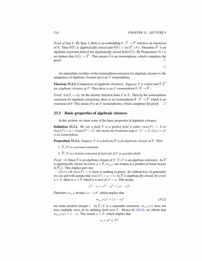
214 CHAPTER 33. LECTURE 9
Proof of Step 4. By Step 3, there is an embedding θ : F→ F′ which is an extension
of θ. Then θ(F) is algebraically closed and θ(F) ∈ Int(F′/F ). Therefore F
′ is analgebraic extension field of the algebraically closed field θ(L). By Proposition 32.1.2,we deduce that θ(L) = F
′. This means θ is an isomorphism, which completes theproof.
An immediate corollary of the isomorphism extension for algebraic closures is theuniqueness of algebraic closures up to an F -isomorphism.
Theorem 33.2.2 (Uniqueness of algebraic closures). Suppose F is a field and F,F′
are algebraic closures of F . Then there is an F -isomorphism θ : F→ F′.
Proof. Let θ := idF be the identity function from F to F . Then by the isomorphismextension for algebraic extensions, there is an isomorphism θ : F → F
′ which is anextension of θ. This means θ is an F -isomorphsims, which completes the proof.
33.3 Basic properties of algebraic closures
In this section, we show some of the basic properties of algebraic closures.
Definition 33.3.1. We say a field F is a perfect field if either char(F ) = 0 orchar(F ) = p > 0 and F p = F ; this means the Frobenius map φ : F → F, φ(a) := ap
is an isomorphism.
Proposition 33.3.2. Suppose F is a field and F is an algebraic closure of F . Then
1. F /F is a normal extension.
2. F /F is a Galois extension if and only if F is a perfect field.
Proof. (1) Since F is an algebraic closure of F , F /F is an algebraic extension. As Fis algebraically closed, for every α ∈ F, mα,F can written as a product of linear factorsin F[x]. This implies part one.
(2) (⇒) If char(F ) = 0, there is nothing to prove. So without loss of generalitywe can and will assume that char(F ) = p > 0. As F is algebraically closed, for everya ∈ F , there is α ∈ F which is a zero of xp − a. This means
xp − a = xp − αp = (x− α)p.
Therefore mα,F divides (x− α)p, which implies that
mα,F (x) = (x− α)i (33.2)
for some positive integer i. As F /F is a separable extension, mα,F (x) does nothave multiple zeros in its splitting field over F . Hence by (33.2), we obtain thatmα,F (x) = x− α. This means α ∈ F , which implies that
a = αp ∈ F p.

33.3. BASIC PROPERTIES OF ALGEBRAIC CLOSURES 215
Since this is true for every a ∈ F , we deduce that F = F p.(⇐) If char(F) = 0, then by Theorem 27.3.5 F /F is a separable extension.
Hence together with part (1), we conclude that F /F is a Galois extension. Supposechar(F ) = p > 0. Every α ∈ F is algebraic over F . By Proposition 27.3.4, there is aseparable irreducible polynomial sα,F (x) ∈ F [x] and a non-negative integer k suchthat mα,F (x) = sα,F (xp
k
). Suppose
sα,F (x) = xm + cm−1xm−1 + · · ·+ c0 ∈ F [x]. (33.3)
Since F p = F , there are di’s in F such that ci = dpi for every i. Therefore by (33.3),we obtain
mα,F (x) =xmpk
+ dpm−1x(m−1)pk + · · ·+ dp0
=(xmpk−1
+ dm−1x(m−1)pk−1
+ · · ·+ d0)p if k > 0. (33.4)
By (33.4), we reach to a contradiction as mα,F (x) ∈ F [x] is irreducible and
xmpk−1
+ dm−1x(m−1)pk−1
+ · · ·+ d0 ∈ F [x].
Hence k = 0, which means mα,F = sα,F . This implies that mα,F ∈ F [x] is separablefor every α ∈ F.
Corollary 33.3.3. A field F is perfect if and only if every algebraic extension E/F isseparable.
Proof. (⇒) Let E be an algebraic closure of E. Then E/F is an algebraic extension asE/E and E/F are algebraic extensions (see Proposition 20.6.1). As E is algebraicallyclosed, we deduce that E is an algebraic closure of F . Therefore by Proposition 33.3.2,E/F is a Galois extension as F is perfect. In particular, E/F is a separable extension.As E ∈ Int(E/F ), we conclude that E/F is a separable extension.
(⇐) Suppose F is an algebraic closure of F . By hypothesis, F /F is separable. Bypart (1) of Proposition 33.3.2, F /F is a normal extension. Hence we conclude thatF /F is a Galois extension. Hence by part (2) of Proposition 33.3.2, we deduce that Fis perfect. This completes the proof.
The next result shows that if add all the zeros of polynomials in F [x] to F , we endup getting an algebraically closed field.
Proposition 33.3.4. Suppose F is a field and F is an algebraic closure of F . Let
Intf,n(F /F ) := {E ∈ Int(F /F ) | E/F is a finite normal extension}.
Then F =⋃E∈Intf,n(F /F )E.
Proof. Every α ∈ F is algebraic over F . Since F is algebraically closed,
mα,F (x) = (x− α1) · · · (x− αn)
for some α1 := α, α2, . . . , αn ∈ F. Let E := F [α1, . . . , αn]. Then E is a splittingfield of mα,F over F . Hence E/F is a finite normal extension (see Proposition 23.1.1).Thus E ∈ Intf,n(F /F ). This completes the proof as α ∈ E.

216 CHAPTER 33. LECTURE 9
33.4 Group of automorphisms of algebraic closures
In this brief section, we briefly outline how AutF (F) looks like where F is analgebraic closure of F .
Lemma 33.4.1. Suppose F is a field, F is an algebraic closure of F , and E ∈Intf,n(F /F ). Let rE : AutF (F) → AutF (E) be the restriction map rE(θ) := θ|E .Then rE is a well-defined surjective group homomorphism and ker rE = AutE(F).
Proof. For every α ∈ E and θ ∈ AutF (F), θ(α) is a zero of mα,F . Since E/F isa normal extension, mα,F decomposes into linear factors in E[x]. Hence θ(α) ∈ E.This implies that rE is well-defined. It is clear that rE is a group homomorphism. Nextwe show that rE is surjective. Suppose θ ∈ AutF (E). Notice that F is algebraicallyclosed and F /E is algebraic, and so F is an algebraic closure of E. Therefore bythe isomorphism extension for algebraically closed (see Theorem 33.2.1), there is anisomorphism θ : F→ F which is an extension of θ. Notice that θ is an F -isomorphism,so is θ. Therefore θ ∈ AutF (F) and θ = rE(θ). This shows that rE is surjective.Finally suppose θ ∈ ker rE . This means θ|E = idE , which implies that θ ∈ AutE(F).This completes the proof.
If E,E′ ∈ Intf,n(F /F ) and E ⊆ E′, then by a similar argument as in the proofof Lemma 33.4.1 we have that
rE′,E : AutF (E′)→ AutF (E), rE′,E(θ) := θ|E
is a well-defined group homomorphism. Notice that
rE = rE′,E ◦ rE′ . (33.5)
Lemma 33.4.2. Suppose F is a field, F is an algebraic closure of F . Let
r : AutF (F)→∏
E∈Intf,n(F /F )
AutF (E), r(θ) := (rE(θ)).
Then r is an injective group homomorphism.
Proof. Since rE’s are group homomorphisms, r is a group homomorphism. Suppose θis in the kernel of r. Then for every E ∈ Intf,n(F /F ), we have θ|E = idE . Thereforeby Proposition 33.3.4, we have θ = id. This completes the proof.
Next we want to understand the image of r. By (33.5), we have that the image of ris a subset of
G(F /F ) := {(θE) | ∀E ⊆ E′, E,E′ ∈ Intf,n(F /F ), rE′,E(θE′) = θE}.
In fact one can show that the image of r isG(F /F ), which implies the following result.
Theorem 33.4.3. Suppose F is a field and F is an algebraic closure of F . Thenr : AutF (F)→ G(F /F ) is an isomorphism.

33.4. GROUP OF AUTOMORPHISMS OF ALGEBRAIC CLOSURES 217
I leave the proof of Theorem 33.4.3 as an exercise. Here are the steps for provingthe surjectivity of r. Suppose (θE) ∈ G(F /F ). Let θ : F→ F be θ(α) := θE(α) ifα ∈ E and E ∈ Intf,n(F /F ).
1. Show that θ is well-defined. To show this notice that if E1, E2 ∈ Intf,n(F /F ),then there is E3 ∈ Intf,n(F /F ) such that E1, E2 ⊆ E3.
2. Show that θ is a homomorphism, and then prove that θ is an F -automorphism.
3. Finally observe that r(θ) = (θE).


Chapter 34
Lecture 10
34.1 Galois correspondence for algebraic closures
Suppose F is a field and F is an algebraic closure of F . By Proposition 33.3.2, wehave that F /F is a Galois extension if and only if F is perfect. So we assume that Fis perfect, and investigate how much Galois’s correspondence between Int(F /F ) andSub(AutF (F)) hold. As in the fundamental theorem of Galois theory, we let
Ψ : Int(F /F )→ Sub(AutF (F)), Ψ(E) := AutE(F), (34.1)
andΦ : Sub(AutF (F))→ Int(F /F ), Φ(H) := Fix(H). (34.2)
Proposition 34.1.1. Suppose F is a field and F is an algebraic closure of F . Then forevery E ∈ Int(F /F ), we have
Fix(AutE(F)) = E.
Proof. ClearlyE ⊆ Fix(AutE(F)). Suppose to the contrary thatα is in Fix(AutE(F))but not in E. Hence degmα,E ≥ 2. Suppose α′ ∈ F is another zero of mα,E . Hencethere is an E-isomorphism θ : E[α]→ E[α′]. Notice that F is an algebraic closure ofE[α] and E[α′]. Therefore by the isomorphism extension for algebraic closures (seeTheorem 33.2.1), there is an isomorphism θ : F→ F which is an extension of θ. Thisimplies that θ ∈ AutE(F) and θ(α) = α′. Therefore α is not in Fix(AutE(F)), whichis a contradiction.
By Proposition 34.1.1, we have Φ ◦Ψ = id. Therefore Ψ and Φ are inverse of eachother from Int(F /F ) to the image of Ψ
{AutE(F) | E ∈ Int(F /F )}.
Later we will see that there are a lot of subgroups of AutF (F) which are not in theimage of Ψ. One can define a topology on AutF (F) called the Krull topology and withrespect to this topology the image of Ψ consists of all closed subgroups of AutF (F).We do not go to the definition of the Krull topology here, but we refer to the image ofΨ as the closed subgroups of AutF (F).
219

220 CHAPTER 34. LECTURE 10
Proposition 34.1.2. Let Ψ and Φ be as in (34.1) and (34.2). Then Ψ and Φ inducebijections between
{E ∈ Int(F /F ) | E/F is a normal extension}, and
{N ∈ Sub(AutF (F)) | N is a normal closed subrgoup}.
Moreover if E/F is a normal extension, then
AutF (F)
AutE(F)' AutF (E).
Proof. Suppose E/F is a normal extension. We want to show that AutE(F) is anormal subgroup of AutF (F). For every θ ∈ AutF (F) and α ∈ E, θ(α) is anotherzero ofmα,F . Since E/F is a normal extension, θ(α) is in E. Therefore the restrictionmap
rE : AutF (F)→ AutF (E), rE(θ) := θ|E
is a well-defined function. It is clear that rE is a group homomorphism. By defini-tion, we have that ker rE = AutE(F). Therefore AutE(F) is a normal subgroup ofAutF (F). Notice that F is an algebraic closure ofE as well. Hence by the isomorphismextension theorem for algebraic closures (see Theorem 33.2.1), every θ ∈ AutF (E)
can be extended to an element θ ∈ AutF (F). This means rE is surjective. Thus by thefirst isomorphism theorem for groups, we have
AutF (F)
AutE(F)' AutF (E).
Next let’s assume that N is a normal subgroup of AutF (F). We want to show thatFix(N)/F is a normal extension. Suppose α ∈ Fix(N). We want to show mα,F canbe decomposed into linear factors in (Fix(N))[x]. As F is algebraically closed, thereare
α1 := α, α2, . . . , αn ∈ F
such thatmα,F (x) = (x− α1) · · · (x− αn).
Hence, for all i, by Lemma 16.2.2, there is an F -isomorphism θi : F [α1]→ F [αi] suchthat θi(α1) = αi. Notice that F is an algebraic closure of F [αj ] for every j. Hence bythe isomorphism extension theorem for algebraic closures (see Theorem 33.2.1), thereare θi : F→ F such that θi|F [α1] = θi. In particular, θi ∈ AutF (F) and θi(α1) = αi.
We want to use θi(α1) = αi, α1 ∈ Fix(N), and N E AutF (F) to show αi ∈Fix(N).
This means we want to show that σ(αi) = αi for every σ ∈ N . The equalityσ(αi) = αi holds if and only if
σ(θi(α1)) = θi(α1). (34.3)
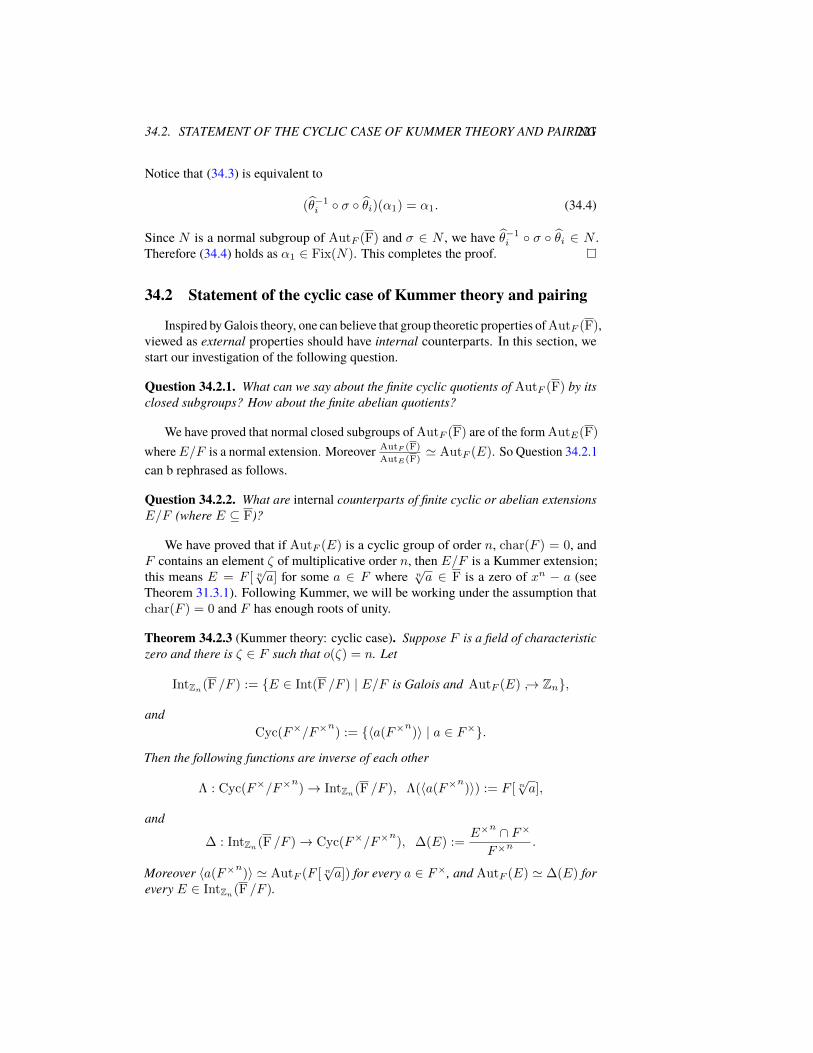
34.2. STATEMENT OF THE CYCLIC CASE OF KUMMER THEORY AND PAIRING221
Notice that (34.3) is equivalent to
(θ−1i ◦ σ ◦ θi)(α1) = α1. (34.4)
Since N is a normal subgroup of AutF (F) and σ ∈ N , we have θ−1i ◦ σ ◦ θi ∈ N .
Therefore (34.4) holds as α1 ∈ Fix(N). This completes the proof.
34.2 Statement of the cyclic case of Kummer theory and pairing
Inspired by Galois theory, one can believe that group theoretic properties of AutF (F),viewed as external properties should have internal counterparts. In this section, westart our investigation of the following question.
Question 34.2.1. What can we say about the finite cyclic quotients of AutF (F) by itsclosed subgroups? How about the finite abelian quotients?
We have proved that normal closed subgroups of AutF (F) are of the form AutE(F)
whereE/F is a normal extension. Moreover AutF (F)
AutE(F)' AutF (E). So Question 34.2.1
can b rephrased as follows.
Question 34.2.2. What are internal counterparts of finite cyclic or abelian extensionsE/F (where E ⊆ F)?
We have proved that if AutF (E) is a cyclic group of order n, char(F ) = 0, andF contains an element ζ of multiplicative order n, then E/F is a Kummer extension;this means E = F [ n
√a] for some a ∈ F where n
√a ∈ F is a zero of xn − a (see
Theorem 31.3.1). Following Kummer, we will be working under the assumption thatchar(F ) = 0 and F has enough roots of unity.
Theorem 34.2.3 (Kummer theory: cyclic case). Suppose F is a field of characteristiczero and there is ζ ∈ F such that o(ζ) = n. Let
IntZn(F /F ) := {E ∈ Int(F /F ) | E/F is Galois and AutF (E) ↪→ Zn},
andCyc(F×/F×
n) := {〈a(F×
n)〉 | a ∈ F×}.
Then the following functions are inverse of each other
Λ : Cyc(F×/F×n)→ IntZn(F /F ), Λ(〈a(F×
n)〉) := F [ n
√a],
and
∆ : IntZn(F /F )→ Cyc(F×/F×n), ∆(E) :=
E×n ∩ F×
F×n.
Moreover 〈a(F×n)〉 ' AutF (F [ n
√a]) for every a ∈ F×, and AutF (E) ' ∆(E) for
every E ∈ IntZn(F /F ).

222 CHAPTER 34. LECTURE 10
Proof of Theorem 34.2.3 is based on the following function which is called aKummer pairing. Let
f : AutF (E)×∆(E)→Mn, f(σ, a) :=σ(α)
α, (34.5)
where a := αn ∈ F× for someα ∈ E× and a := αn(F×n) andMn := {1, ζ, . . . , ζn−1}.
Lemma 34.2.4. Suppose F is a field of characteristic zero which contains an elementζ of order n. Suppose E/F is an algebraic extension and f is the Kummer pairinggiven in (34.5). Then f is well-defined.
Proof. We need to address two issues: why σ(α)α is in Mn and why it only depends
on a := αn(F×n) and it is independent of the choice of α. Notice that α is a zero of
xn − a. Then α, ζα, . . . , ζn−1α are distinct zeros of xn − a. By the generalized factortheorem, comparing degrees and leading coefficients, we obtain that
xn − a = (x− α)(x− ζα) · · · (x− ζn−1α). (34.6)
As xn− a ∈ F [x], every σ ∈ AutF (E) permutes zeros of xn− a. Hence σ(α) = ζiα
for some integer i in [0, n− 1]. This implies that σ(α)α ∈Mn.
If αn1 (F×n) = αn2 (F×
n) for some α1, α2 ∈ E× with αni ∈ F , then there are
a, c ∈ F× such that αn1 = αn2 cn = a ∈ F×. Hence α1 and cα2 are two zeros of
xn − a. By (34.6), we conclude that α1 = ζicα2 for some integer i in [0, n − 1].Therefore
σ(α1)
α1=σ(ζicα2)
ζicα2=ζicσ(α2)
ζicα2=σ(α2)
α2.
This completes the proof.
Lemma 34.2.5. Suppose F is a field of characteristic zero which contains an elementζ of order n. Suppose E/F is an algebraic extension and f is the Kummer pairinggiven in (34.5). Then f is a group homomorphism with respect to each componentseparately.
Proof. First component. Suppose σ1, σ2 ∈ AutF (E) and a := a(F×n) where a = αn
for some α ∈ E×. Suppose
f(σ1, a) = ζi1 and f(σ2, a) = ζi2 . (34.7)
We want to showf(σ1 ◦ σ2, a) = ζi1 · ζi2 = ζi1+i2 . (34.8)
By (34.7), we have σ1(α) = ζi1α and σ2(α) = ζi2α. Hence
σ1 ◦ σ(α) = σ1(ζi2α) = ζi2σ1(α) = ζi2 · ζi1α = ζi1+i2α.
Therefore σ1◦σ2(α)α = ζi1+i2 which implies (34.8), and this shows that f is a group
homomorphism with respect to the first component.

34.3. FUNCTIONS IN THE CYCLIC CASE OF KUMMER THEORY 223
Second component. Suppose σ ∈ AutF (E) and, for i = 1, 2, ai := ai(F×n)
where ai = αni for some αi ∈ E×. Let
f(σ, a1) = ζi1 and f(σ, a2) = ζi2 . (34.9)
We want to showf(σ, a1 · a2) = ζi1+i2 . (34.10)
By (34.9), we have σ(α1) = ζi1α1 and σ(α2) = ζi2α2. Hence
σ(α1α2) = σ(α1)σ(α2) = ζi1α1 · ζi2α2 = ζi1+i2α1α2.
This implies that σ(α1α2)α1α2
= ζi1+i2 and (34.10) follows. This completes the proof.
By Lemma 34.2.5, we conclude that for σ0 ∈ AutF (E) and a0 ∈ ∆(E),
fa0 : AutF (E)→Mn, fa0(σ) := f(σ, a0) (34.11)
andfσ0 : ∆(E)→Mn, fσ0(a) := f(σ0, a) (34.12)
are group homomorphisms.
34.3 Functions in the cyclic case of Kummer theory
In this section, we prove that the functions Λ and ∆ given in Theorem 34.2.3 arewell-defined. To show Λ(〈a(F×
n)〉) := F [ n
√a] is a well-defined function, we need
to address two issues: F [ n√a] ∈ IntZn(F /F ) and F [ n
√a] depends only on the cyclic
group 〈a(F×n)〉 and it is independent of the choice of a. By Proposition 28.3.2, F [ n
√a]
is in IntZn(F /F ). We go over its prove. By (34.6) and having ζ ∈ F , we conclude thatF [ n√a] is a splitting field of xn − a over F . This implies that F [ n
√a]/F is a normal
extension. As char(F ) = 0, F [ n√a]/F is a separable extension. Hence F [ n
√a]/F is
a Galois extension. Let a := a(F×n). By (34.11), fa(σ) := σ( n
√a)
n√a
is a well-definedgroup homomorphism.
Lemma 34.3.1. Suppose F is a field of characteristic zero and it has an element ζ oforder n. Suppose a ∈ F , n
√a is a zero of xn − a and E := F [ n
√a]. Let
fa : AutF (F [ n√a])→Mn, fa(σ) :=
σ( n√a)
n√a
,
where a := a(F×n). Then fa is a well-defined injective group homomorphism. In
particular, F [ n√a] ∈ IntZn(F /F ).
Proof. By Lemma 34.2.4 and (34.11), fa is a well-defined group homomorphism.Suppose fa(σ) = 1 for some σ ∈ AutF (E). Then σ( n
√a) = n
√a, which implies that
σ = id. This completes the proof.
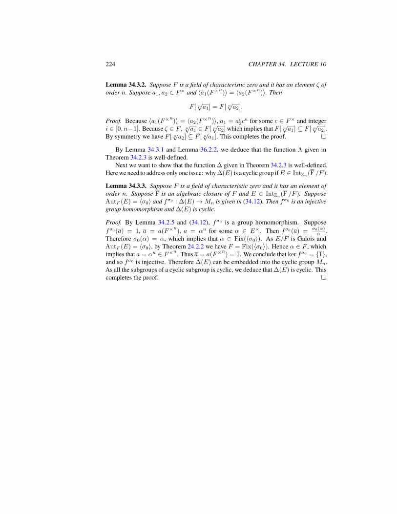
224 CHAPTER 34. LECTURE 10
Lemma 34.3.2. Suppose F is a field of characteristic zero and it has an element ζ oforder n. Suppose a1, a2 ∈ F× and 〈a1(F×
n)〉 = 〈a2(F×
n)〉. Then
F [ n√a1] = F [ n
√a2].
Proof. Because 〈a1(F×n)〉 = 〈a2(F×
n)〉, a1 = ai2c
n for some c ∈ F× and integeri ∈ [0, n−1]. Because ζ ∈ F , n
√a1 ∈ F [ n
√a2] which implies thatF [ n
√a1] ⊆ F [ n
√a2].
By symmetry we have F [ n√a2] ⊆ F [ n
√a1]. This completes the proof.
By Lemma 34.3.1 and Lemma 36.2.2, we deduce that the function Λ given inTheorem 34.2.3 is well-defined.
Next we want to show that the function ∆ given in Theorem 34.2.3 is well-defined.Here we need to address only one issue: why ∆(E) is a cyclic group ifE ∈ IntZn(F /F ).
Lemma 34.3.3. Suppose F is a field of characteristic zero and it has an element oforder n. Suppose F is an algebraic closure of F and E ∈ IntZn(F /F ). SupposeAutF (E) = 〈σ0〉 and fσ0 : ∆(E)→Mn is given in (34.12). Then fσ0 is an injectivegroup homomorphism and ∆(E) is cyclic.
Proof. By Lemma 34.2.5 and (34.12), fσ0 is a group homomorphism. Supposefσ0(a) = 1, a = a(F×
n), a = αn for some α ∈ E×. Then fσ0(a) = σ0(α)
α .Therefore σ0(α) = α, which implies that α ∈ Fix(〈σ0〉). As E/F is Galois andAutF (E) = 〈σ0〉, by Theorem 24.2.2 we have F = Fix(〈σ0〉). Hence α ∈ F , whichimplies that a = αn ∈ F×n. Thus a = a(F×
n) = 1. We conclude that ker fσ0 = {1},
and so fσ0 is injective. Therefore ∆(E) can be embedded into the cyclic group Mn.As all the subgroups of a cyclic subgroup is cyclic, we deduce that ∆(E) is cyclic. Thiscompletes the proof.

Chapter 35
Lecture 11
35.1 Kummer theory: the cyclic case
The main goal of this section is to prove Theorem 34.2.3. In Section 34.3, we haveproved that
Λ : Cyc(F×/F×n)→ IntZn(F /F ), Λ(〈a(F×
n)〉) := F [ n
√a],
and∆ : IntZn(F /F )→ Cyc(F×/F×
n), ∆(E) :=
E×n ∩ F×
F×n
are well-defined. Next we want to prove that ∆ ◦ Λ = id, which is equivalent to
F [ n√a]×
n ∩ F×
F×n= 〈a(F×
n)〉. (35.1)
As ( n√a)n ∈ F××, a(F×
n) is in the left hand side of (35.1). Hence
F [ n√a]×
n ∩ F×
F×n⊇ 〈a(F×
n)〉. (35.2)
Suppose b := b(F×n) ∈ ∆(F [ n
√a]). We want to show that b is in 〈a(F×
n)〉. By
definition of ∆(F [ n√a]), there is β ∈ F [ n
√a]× such that βn(F×
n) = b(F×
n). Hence
by Lemma 36.2.2, F [β] = F [ n√b]. Then F [ n
√b] ∈ Int(F [ n
√a]/F ). Notice that by
Lemma 34.3.1, F [ n√b], F [ n
√a] ∈ IntZn(F /F ) and
fb : AutF (F [n√b])→Mn and fa : AutF (F [ n
√a])→Mn (35.3)
are injective group homomorphisms. On the there hand, by the fundamental theorem ofGalois theory, if σ0 generates AutF (F [ n
√a]), then σ0|F [
n√b] generates AutF (F [ n
√b]).
HenceIm fb = 〈fb(σ0|F [
n√b])〉 and Im fa = 〈fa(σ0)〉, (35.4)
and by (35.3), | Im fb| = |〈σ0|F [n√b]〉| divides | Im fa| = |〈σ0〉|. As Im fb and Im fa
are subgroups of the cyclic groupMn and the order of Im fb divides the order of Im fa,
225

226 CHAPTER 35. LECTURE 11
we conclude that Im fb ⊆ Im fa, which together with (35.4) implies that
fb(σ0|F [n√b]) = fa(σ0)i (35.5)
for some non-negative integer i. By (35.5), we obtain that σ0(n√b)
n√b
=(σ0( n√a)
n√a
)i.
Hence σ0
(n√b
n√ai
)=
n√b
n√ai
, which means thatn√b
n√ai∈ Fix(〈σ0〉). As F [ n
√a]/F is a
Galois,Fix(AutF (F [ n
√a]) = Fix(〈σ0〉) = F.
Altogether, we conclude that n√b = c n
√ai for some c ∈ F×. Therefore
b = b(F×n) = ai(F×
n) ∈ 〈a(F×
n)〉. (35.6)
By (35.6) and (35.2), we obtain that ∆ ◦ Λ = id.Since ∆ ◦ Λ = id, Λ and ∆ induce a bijection between the domain of Λ and the
image of Λ. Hence to show Λ and ∆ are inverse of each other it is enough to show thatΛ is surjective.
For every E ∈ IntZn(F /F ), by Theorem 31.3.1, E = F [ n√a] for some a ∈ F ,
which means E = Λ(〈a(F×n)〉). Therefore Λ is surjective, and so Λ ◦∆ = id.
Next we want to show that AutF (E) ' ∆(E) for every E ∈ IntZn(F /F ).Suppose AutF (E) = 〈σ0〉 and ∆(E) = 〈a0(F×
n)〉. Then by Lemma 34.3.1 and
Lemma 34.3.3,
fa0 : AutF (F [ n√a0])→Mn and fσ0 : ∆(E)→Mn (35.7)
injective group homomorphisms, where a0 := a0(F×n). Therefore
∆(E) '〈fσ0(a0)〉 = 〈f(σ0, a0)〉 andAutF (E) '〈fa0(σ0)〉 = 〈f(σ0, a0)〉. (35.8)
By (35.8), we conclude that ∆(E) ' AutF (E). Finally, we have
AutF (F [ n√a]) ' ∆(F [ n
√a]) = ∆ ◦ Λ(〈a(F×
n)〉) = 〈a(F×
n)〉,
which completes the proof of Theorem 34.2.3.
35.2 Dual of abelian groups
Our next goal is to prove the abelian case of Kummer theory. To prove this result, weneed to study dual of finite abelian groups and show further properties of the Kummerpairing. In this section, we introduce the dual of a finite abelian group, and prove someof its basic properties. It is worth pointing out that some of these properties can beproved using classification of finite abelian groups in a more straightforward fashion.Here, however, we present an approach that avoids using the classification of finiteabelian groups.
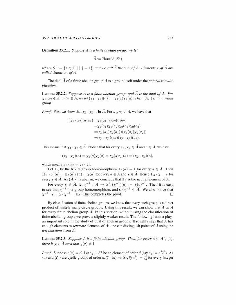
35.2. DUAL OF ABELIAN GROUPS 227
Definition 35.2.1. Suppose A is a finite abelian group. We let
A := Hom(A,S1)
where S1 := {z ∈ C | |z| = 1}, and we call A the dual of A. Elements χ of A arecalled characters of A.
The dual A of a finite abelian group A is a group itself under the pointwise multi-plication.
Lemma 35.2.2. Suppose A is a finite abelian group, and A is the dual of A. Forχ1, χ2 ∈ A and a ∈ A, we let (χ1 · χ2)(a) := χ1(a)χ2(a). Then (A, ·) is an abeliangroup.
Proof. First we show that χ1 · χ2 is in A. For a1, a2 ∈ A, we have that
(χ1 · χ2)(a1a2) =χ1(a1a2)χ2(a1a2)
=χ1(a1)χ1(a2)χ2(a1)χ2(a2)
=(χ1(a1)χ2(a1))(χ1(a2)χ2(a2))
=(χ1 · χ2)(a1)(χ1 · χ2)(a2).
This means that χ1 · χ2 ∈ A. Notice that for every χ1, χ2 ∈ A and a ∈ A, we have
(χ1 · χ2)(a) = χ1(a)χ2(a) = χ2(a)χ1(a) = (χ2 · χ1)(a),
which means χ1 · χ2 = χ2 · χ1.Let 1A be the trivial group homomorphism 1A(a) = 1 for every a ∈ A. Then
(1A · χ)(a) = 1A(a)χ(a) = χ(a) for every a ∈ A and χ ∈ A. Hence 1A · χ = χ forevery χ ∈ A. As (A, ·) is abelian, we conclude that 1A is the neutral element of A.
For every χ ∈ A, let χ−1 : A → S1, (χ−1)(a) := χ(a)−1. Then it is easyto see that χ−1 is a group homomorphism, and so χ−1 ∈ A. We also notice thatχ−1 · χ = χ · χ−1 = 1A. This completes the proof.
By classification of finite abelian groups, we know that every such group is a directproduct of finitely many circle groups. Using this result, we can show that A ' Afor every finite abelian group A. In this section, without using the classification offinite abelian groups, we prove a slightly weaker result. The following lemma playsan important role in the study of dual of abelian groups. It roughly says that A hasenough elements to separate elements of A: one can distinguish points of A using thetest functions from A.
Lemma 35.2.3. Suppose A is a finite abelian group. Then, for every a ∈ A \ {1},there is χ ∈ A such that χ(a) 6= 1.
Proof. Suppose o(a) = d. Let ζd ∈ S1 be an element of order d (say ζd := e2πid ). As
〈a〉 and 〈ζd〉 are cyclic groups of order d, χ : 〈a〉 → S1, χ(ai) := ζid for every integer
228 CHAPTER 35. LECTURE 11
i is an injective group homomorphism (and Imχ) is the cyclic group 〈ζd〉). We willshow that χ has an extension χ ∈ A; in particular, χ(a) = χ(a) = ζd 6= 1. Let
Σ := {(H,χ) | H ≤ A, a ∈ H,χ ∈ H, χ|〈a〉 = χ}.
Notice that (〈a〉, χ) ∈ Σ, and so Σ is non-empty. Let’s also point out that Σ is a finiteset. This is the case because for every χ ∈ A and a′ ∈ A,
χ(a′)|A| = χ(a′|A|) = χ(1) = 1,
and so χ(a′) has at most |A|-many possibilities for every a′ ∈ A. Our goal is to showthat there is (A,χ) in Σ; this means we are looking for a largest possible elementof in Σ. To make sense of this, we introduce the following partial order on Σ. For(H1, χ1), (H2, χ2) ∈ Σ, we say (H1, χ1) 4 (H2, χ2) if H1 ≤ H2 and χ2|H2 . It iseasy to see that Σ is a poset with respect to 4. As Σ is a non-empty finite set, it has amaximal element. Suppose (H,χ) is a maximal element of Σ. We can finish the proofby showing that H = A.
Suppose to the contrary that there is a′ ∈ A \ H . We want to extend χ to anelement χ′ ∈ 〈H, a′〉 where 〈H, a′〉 is the group generated by a and H . Notice that ifwe manage to extend χ to a character of 〈H, a′〉, this would contradict the maximalityof (H,χ) in Σ.
To extend χ to a character of 〈H, a′〉, we start by describing elements of 〈H, a′〉.Since A is abelian, every subgroup is normal. So we can consider the quotient groupA/H . As H is in the kernel of the quotient map pH : A→ A/H , we have that
pH(〈H, a′〉) = 〈pH(a′)〉 = 〈a′H〉 = {a′iH | i = 0, 1, . . . , d− 1} (35.9)
where d is the order of a′H in A/H . Because cosets of H in 〈H, a′〉 is a partitionof 〈H, a′〉, we conclude that every element of 〈H, a′〉 can be written as a′ih for someinteger i in [0, d− 1] and h ∈ H .
Next we notice that to find an extension χ′ of χ in 〈H, a′〉, we only need to finda suitable choice for χ′(a′). Since pH(a′)d = pH(1), a′d = h0 for some h0 ∈ H .Therefore for every possible extension χ′ of χ, we have
χ′(a′)d = χ′(a′d) = χ′(h0) = χ(h0). (35.10)
Hence χ′(a′) should be a zero of xd − χ(h0). Since h0 is of finite order, χ(h0) is aroot of unity and so all the zeros of xd − χ(h0) are also roots of unity; in particularthey are in S1. Suppose ζ 6= 1 is a zero of xd − χ(h0), and let
χ′(aih) := ζiχ(h)
for every integer i and h ∈ H . We want to show that χ′ is a well-defined extension ofχ.
Suppose a′i1h1 = a′i2h2 for some integers i1, i2 and h1, h2 ∈ H . We have toshow that ζi1χ(h1) = ζi2χ(h2). Because a′i1h1 = a′i2h2, we have a′i1−i2 = h2h
−11 .

35.2. DUAL OF ABELIAN GROUPS 229
Therefore pH(a′)i1−i2 = pH(1) as h2h−11 ∈ H . This implies that the order of pH(a′)
divides i1 − i2, and so i1−i2d is an integer. Hence
h2h−11 = a′i1−i2 = (a′d)
i1−i2d = h
i1−i2d
0 . (35.11)
By (35.11), we conclude that
χ(h2h−11 ) = χ(h
i1−i2d
0 ) = χ(h0)i1−i2d = (ζd)
i1−i2d = ζi1−i2 .
Hence ζi1χ(h1) = ζi2χ(h2), which implies that χ′ is well-defined.Next we check that χ′ is a group homomorphism. Suppose g, g′ ∈ 〈a,H〉. Then
g = aih and g′ = ai′h′ for some integers i, i′ and h, h′ ∈ H . Therefore
χ′(gg′) = χ′((aih)(ai′h′)) = χ′(ai+i
′hh′) = ζi+i
′χ(hh′), (35.12)
and
χ′(g)χ′(g′) = χ′(aih)χ′(ai′h′) = (ζiχ(h))(ζi
′χ(h′)) = ζi+i
′χ(h)χ(h′). (35.13)
By (35.12) and (35.13), we conclude thatχ′ is a group homomorphism. Clearlyχ′(h) =χ(h) for every h ∈ H and χ′(a) = ζ 6= 1. Altogether, we have (〈a,H〉, χ′) ∈ Σ,(H,χ) 4 (〈a,H〉, χ′), andH 6= 〈a,H〉. This is a contradiction as (H,χ) is a maximalelement of Σ. This completes the proof.

Chapter 36
Lecture 12
36.1 Dual of abelian groups
Lemma 35.2.3 shows us that A has plenty of elements to separate points of A. Thenext lemma says that the order of A cannot be more than the order of A.
Lemma 36.1.1. Suppose A is a finite abelian group and A is its dual. Then |A| ≤ |A|.
Proof. We proceed by strong induction on |A|. Since A is a finite group, it has amaximal subgroup M . As A is abelian, every subgroup is normal and we can considerthe quotient group A/M . Because of the bijection between subgroups of A/M andsubgroups of A that contain M as a subgroup (see Proposition 30.1.2)and maximalityof M , we deduce that A/M does not have a non-trivial proper subgroup. HenceA/M is a cyclic group of prime order (see Lemma 30.1.3); say |A/M | = p. SupposeA/M = 〈aM〉 and ap = b; then b ∈M . Every χ ∈ A is uniquely determined by χ|Mand χ(a). Notice that χ|M ∈ M . Suppose χ|M = χ ∈ M ; then
χ(a)p = χ(ap) = χ(b) = χ(b).
Hence χ(a) is a zero of xp − χ(b). This means for a given χ, χ(a) has at most ppossibilities. Altogether we conclude that
|A| =∑χ∈A
1 =∑χ∈M
( ∑ζ is a zero of xp−χ(b)
∑χ∈A,χ|M=χ,χ(a)=ζ
1)
≤∑χ∈M
( ∑ζ is a zero of xp−χ(b)
1)≤∑χ∈M
p = p|M |
≤p|M | = |A|,
where the last inequality holds because of the strong induction hypothesis. This com-pletes the proof.
Now we are ready to prove our main result on dual of abelian groups.
231

232 CHAPTER 36. LECTURE 12
Theorem 36.1.2. SupposeA is a finite abelian group and A is its dual. Then |A| = |A|and
` : A→ A, (`(a))(χ) := χ(a)
is an isomorphism.
Recall that A consists of functions on A, and `(a) can be viewed as an evaluationat a map.
Proof. First we start by showing that ` is a well-defined function. For every a ∈ A, let`a : A→ S1 be the evaluation at a map; that means
`a(χ) := χ(a).
We claim that `a is a group homomorphism and so it belongs to the dual of A. Forevery χ1, χ2 ∈ A, we have
`a(χ1 · χ2) = (χ1 · χ2)(a) = χ1(a)χ2(a) = `a(χ1)`a(χ2),
and so `a ∈A. Next we show that a 7→ `a is a group homomorphism from A to A. For
every a1, a2 ∈ A and χ ∈ A, we have
`a1a2(χ) = χ(a1a2) = χ(a1)χ(a2) = `a1(χ)`a2(χ) = (`a1 · `a2)(χ),
and so `a1a2 = `a1 · `a2 for every a1, a2 ∈ A. This implies that
` : A→ A, `(a) := `a
is a group homomorphism. At this step, we show that ` is injective. To show this, it isnecessary and sufficient that `(a) 6= 1A if a 6= 1. For a 6= 1, by Lemma 35.2.3, thereis χ ∈ A such that χ(a) 6= 1. Hence `a(χ) 6= 1, which means (`(a))(χ) 6= 1. Thus`(a) 6= 1A, which implies that ` is injective. In particular, we have
|A| ≤ | A|. (36.1)
On the other hand, by Lemma 36.1.1, we have
| A| ≤ |A| ≤ |A|. (36.2)
By (36.1) and (36.2), we conclude that
|A| = |A| = | A|. (36.3)
As ` : A→ A is an injective group homomorphism and |A| = |A|, we deduce that ` is
an isomorphism. This completes the proof.

36.2. STATEMENT OF FINITE ABELIAN CASE OF KUMMER THEORY 233
We finish our discussion of dual of abelian groups by looking at the characters ofan abelian group of exponent n.
Suppose A is a finite abelian group whose exponent divides n; that means an = 1for every a ∈ A. Then for every χ ∈ A and a ∈ A, we have
χ(a)n = χ(an) = χ(1) = 1,
and so χ(a) = e2πkin for some integer k. This means A is the same as Hom(A, 〈ζn〉)
where ζn := e2πin . Therefore, if F is a field which contains an element ζ of order n,
then for every abelian group A of exponent n the dual A of A can be identified withHom(A,Mn) where Mn := 〈ζ〉.
Let’s also observe that if A is a finite abelian group whose exponent divides n, thenthe exponent of A is also a divisor of n. This holds because
(χn)(a) = χ(a)n = χ(an) = χ(1) = 1
for every a ∈ A.
36.2 Statement of finite abelian case of Kummer theory
In this section, we state the finite abelian case of Kummer theory and prove that theinvolved functions are well-defined. In this section F is a field and F is an algebraicclosure of F . Let Intab,n(F /F ) be the set of all E ∈ Int(F /F ) such that E/F is afinite Galois extension and AutF (E) is an abelian group of exponent n, and
Subf(F×/F×
n) := {A ≤ F×/F×n | A is finite}.
Theorem 36.2.1 (Kummer theory: abelian case). Suppose F is a field of characteristiczero which contains an element of order n. Suppose F is an algebraic closure of F . Let
Λ : Subf(F×/F×
n)→ Intab,n(F /F ), Λ(A) := F [ n
√ai | ai(F×
n) ∈ A]
where n√ai ∈ F is a zero of xn − ai, and
∆ : Intab,n(F /F )→ Subf(F×/F×
n), ∆(E) := (E×
n ∩ F×)/F×n.
Then Λ and ∆ are inverse of each other. Moreover for every E ∈ Intab,n(F /F ),
AutF (E) ' ∆(E).
In the proof, we give a concrete isomorphism between AutF (E) and ∆(E). Westart by showing that Λ and ∆ are well-defined.
Lemma 36.2.2. In the above setting, Λ is well-defined.
Proof. To show Λ is well-defined, we have to show why F [ n√ai | ai(F×
n) ∈ A] is in
Intab,n(F /F ), why it does not depend on the choice of coset representatives ai’s andn√ai.

234 CHAPTER 36. LECTURE 12
SupposeA := {a1(F×n), . . . , am(F×
n)} and n
√ai ∈ F is a zero of xn−ai. Then
g(x) :=∏mi=1(xn − ai) can be written as
g(x) =
m∏i=1
n−1∏j=0
(x− ζj n√ai).
Hence F [ζj n√ai | 1 ≤ i ≤ m, 0 ≤ j < n] is a splitting field of g over F . Notice that
F [ζj n√ai | 1 ≤ i ≤ m, 0 ≤ j < n] = F [ n
√a1, . . . , n
√am]
as ζ ∈ F . Hence F [ n√a1, . . . , n
√am]/F is a finite normal extension. Since char(F ) =
0, every algebraic extension of F is separable. Hence F [ n√a1, . . . , n
√am]/F is a finite
Galois extension. Let E := F [ n√a1, . . . , n
√am] and ai := ai(F
×n). By the Kummerpairing and (34.11),
fA : AutF (E)→Mn × · · · ×Mn, fA(σ) := (fa1(σ), . . . , fam(σ))
is a group homomorphism.Claim. fA is injective.
Proof of Claim. Suppose fA(σ) = (1, . . . , 1). Then, for every i, fai(σ) = 1, whichmeans σ( n
√ai) = n
√ai. Since E = F [ n
√a1, . . . , n
√am], we conclude that σ = id.
The claim follows.
By the above Claim, we deduce that AutF (E) can be embedded inMn×· · ·×Mn,and so AutF (E) is an abelian group of exponent n.
Finally, let’s assume that ai(F×n) = a′i(F
×n) for every i. We have to show that
F [ n√a1, . . . , n
√am] = F [ n
√a′1, . . . ,
n√a′m].
Since ai(F×n) = a′i(F
×n), a′i = aidni for some di ∈ F×. Hence n
√a′i and n
√aidi
are zeros of xn − a′i. As ζ ∈ F , we obtain that n√a′i = ci n
√ai for some ci ∈ F×.
Hence
F [ n√a′i | 1 ≤ i ≤ m] = F [ci n
√ai | 1 ≤ i ≤ m] = F [ n
√ai | 1 ≤ i ≤ m].
This completes the proof.
Lemma 36.2.3. In the above setting ∆ is well-defined.
Proof. We need to show that ∆(E) is a finite group. Suppose
AutF (E) := {σ1, . . . , σk}.
By the Kummer pairing and (34.12),
fE : ∆(E)→Mn × · · · ×Mn, fE(a) := (fσ1(a), . . . , fσk(a)).
Claim. fE is injective.
36.3. KUMMER PAIRING IS A PERFECT PAIRING 235
Proof of Claim. Suppose fE(a) = (1, . . . , 1) where a = a(F×n) and a = αn for
some α ∈ E×. Then, for every i, fσi(a) = 1, which implies that σi(α)α = 1. Therefore
α is in Fix(AutF (E)). Since E/F is a finite Galois extension, Fix(AutF (E)) = F .Hence α ∈ F . Therefore a = (αn)(F×
n) = F×
n= 1 ∈ F×/F×n. This completes
the proof of injectivity of fE .
By the above Claim, ∆(E) can be embedded into Mn × · · · ×Mn, and so it isfinite. This completes the proof.
36.3 Kummer pairing is a perfect pairing
We have proved that Λ and ∆ given in Theorem 36.2.1 are well-defined (seeLemma 36.2.2 and Lemma 36.2.3). The main step to show Λ and ∆ are inverseis the following proposition.
Proposition 36.3.1. Suppose E ∈ Intab,n(F /F ) and let f be the Kummer pairinggiven in (34.5). Then f is a perfect pairing; that means
f : ∆(E)→ AutF (E), (f(a)(σ) := fa(σ) = f(σ, a)
is an isomorphism.
Proof. We start by noticing that by (34.11), fa ∈ AutF (E). For every a1, a2 ∈ ∆(E),(f(a1a2)
)(σ) =f(σ, a1a2)
=f(σ, a1)f(σ, a2)
=(f(a1)
)(σ)(f(a2)
)(σ),
which means f(a1a2) = f(a1) · f(a2). Hence f is a group homomorphism.Next, we show that f is injective. Suppose f(a) = 1. Then for every σ ∈ AutF (E),
(f(a))(σ) = 1, which means f(σ, a) = 1. Notice that f(σ, a) = σ(α)α where α ∈ E×
is a zero of xn − a. Hence σ(α) = α for every σ ∈ AutF (E). Therefore α ∈Fix(AutF (E)), which implies that α ∈ F as E/F is a finite Galois extension. Thusa = αn(F×
n) = 1. This implies that f is injective.
Finally we want to show that f is surjective. Suppose χ ∈ AutF (E). This meansχ : AutF (E) → Mn is a group homomorphism. Let N := kerχ. Then by thefundamental theorem of Galois theory, K := Fix(N) ∈ Int(E/F ), K/F is a Galoisextension, N = AutK(E), and
AutF (K) ' AutF (E)
AutK(E). (36.4)
As AutK(E) = kerχ, by the first isomorphism theorem for groups and (36.4) we have
AutF (K) ' Imχ ≤Mn. (36.5)

236 CHAPTER 36. LECTURE 12
By (36.5), K ∈ IntZn(F /F ). Hence by the surjectivity of Λ from the cyclic case ofKummer theory (see Theorem 34.2.3), we have that K = F [ n
√b]] for some n
√b ∈ E
and b ∈ F . Let b := b(F×n) ∈ ∆(E). Then for every σ ∈ AutF (E), we have
(f(b))(σ) = f(σ, b) = fb(σ|F [n√b]). (36.6)
By (36.6), we conclude that Im f(b) = Im fb, and so it is a cyclic subgroup of Mn.Moreover, by Lemma 34.3.1 and (36.5), we have
| Im f(b)| = | Im fb| = |AutF (F [n√b])| = |AutF (K)| = | Imχ|. (36.7)
As Im f(b) and Imχ are subgroups of the cyclic group Mn and they have the sameorder, we conclude that
Im f(b) = Imχ. (36.8)
Since AutF (K) is cyclic and the restriction map from AutF (E) to AutF (K) is sur-jective, there is σ0 ∈ AutF (E) such that AutF (K) is generated by σ0|K . Hence
Im f(b) = Im fb =⟨σ0( n
√b)
n√b
⟩. (36.9)
We also notice that if σ|K = σ′|K , then (σ−1 ◦ σ ∈ AutK(E). Because kerχ =AutK(E), we conclude that χ(σ) = χ(σ′). Hence
Imχ = 〈χ(σ0)〉. (36.10)
By (36.8), (36.9), and (36.10), we conclude that
χ(σ0) =(σ0( n
√b)
n√b
)i(36.11)
for some integer i such that gcd(i,m) = 1, where m := | Im f(b)|. Hence by (36.11),we obtain that
χ(σ0) = fbi(σ0|K). (36.12)
For every σ ∈ AutF (E), σ|K = σj0|K for some integer j. Therefore σ = σj0τ forsome τ ∈ AutK(E). Notice that kerχ = AutK(E), and so
χ(σ) =χ(σj0τ) = χ(σ0)j
=fbi(σ0|K)j = f
bi(σj0|K)
=fbi(σ|K) =
(f(b
i))
(σ).
This means f(bi) = χ. Therefore f is surjective. This completes the proof that the
Kummer pairing f is a perfect pairing.
36.4. PERFECT PAIRINGS 237
36.4 Perfect pairings
The main goal of this section is to prove the following property of perfect pairings.We formulate this result only for the Kummer pairing.
Proposition 36.4.1. In the setting of Theorem 36.2.1, let A := AutF (E) and B :=∆(E). Let f : A×B → S1 be the Kummer pairing given in (34.5). Let
f : A→ B, (f(a))(b) := f(a, b).
Then f is an isomorphism.
Proof. Notice that by (34.12), f(a) ∈ B. For every a1, a2 ∈ A and b ∈ B, we have
(f(a1a2))(b) =f(a1a2, b) = f(a1, b)f(a2, b)
=(f(a1))(b)(f(a2))(b)
=(f(a1) · f(a2))(b),
and so f(a1a2) = f(a1) · f(a2). This means that f : A → B is a group homomor-phism.
Next we show that f is injective. Suppose to the contrary that there is a 6= 1 suchthat f(a) = 1. Then for every b ∈ B, we have
f(a, b) = 1. (36.13)
Since a 6= 1, by Lemma 35.2.3, there is χ0 ∈ A such that
χ0(a) 6= 1. (36.14)
Since by Proposition 36.3.1 f : B → A is surjective, there is b0 ∈ B such thatf(b0) = χ0. Hence
χ0(a) = (f(b0))(a) = f(a, b0). (36.15)
By (36.13), (36.14), and (36.15), we get a contradiction. This shows that f is injective.Since f : B → A is an isomorphism,
|B| = |A|. (36.16)
By Theorem 36.1.2, we have that
|A| = |A| and |B| = |B|. (36.17)
By (36.16) and (36.17), we deduce that |A| = |B|. As f : A → B is injective and|A| = |B|, we conclude that f is a bijection, and so it is an isomorphism. This completesthe proof.
238 CHAPTER 36. LECTURE 12
36.5 Proof of Kummer theory: abelian case
In this section, we finish the proof of Theorem 36.2.1. We start by proving thatΛ◦∆ = id. Suppose ∆(E) = {a1(F×
n), . . . , am(F×
n)}. We have to show thatE =
F [ n√a1, . . . , n
√am]. Since ai(F×
n) ∈ ∆(E), there is αi ∈ E such that ai(F×
n) =
αni (F×n). Hence ai = αni c
ni for some ci ∈ F×. Therefore n
√ai = (ζjci)αi for some
integer j. Because ζj ∈ F , we conclude that n√ai ∈ E. Therefore
F [ n√a1, . . . , n
√am] ⊆ E. (36.18)
Suppose σ ∈ AutF [ n√a1,..., n
√am](E). Then σ( n
√ai) = n
√ai for every i. This implies
that f(σ, ai) = 1 where ai := ai(F×n). This means f(σ) = 1. By Proposition 36.4.1,
f is an isomorphism, and so σ = id. Hence AutF [ n√a1,..., n
√am](E) = {id}. Therefore
by the fundamental theorem of Galois theory, we have E = F [ n√a1, . . . , n
√am]. This
shows that Λ ◦∆ = id.Next we show that ∆ ◦ Λ = id. Suppose
A := {a1(F×n), . . . , am(F×
n)} ≤ F×/F×n
andE := Λ(A) = F [ n
√a1, . . . , n
√am].
We have to show that ∆(E) = A.For every i, n
√ain ∈ E×n ∩ F×, and so A ⊆ ∆(E).
Suppose to the contrary that A ( ∆(E). Then by Theorem 36.1.2, (∆(E)A ) 6= 1.
So there is a non-trivial group homomorphism χ0 : ∆(E)A → S1. Let
χ0 : ∆(E)→ S1, χ0(x) := χ(xA).
Then A ⊆ kerχ0. Since by Proposition 36.4.1 f : AutF (E) → ∆(E) is an isomor-phism, there is σ0 ∈ AutF (E) such that f(σ0) = χ0. Therefore, for every a ∈ ∆(E),we have
f(σ0, a) = (f(σ0))(a) = χ0(a). (36.19)
By (36.19) and A ⊆ kerχ0, we conclude that f(σ0, ai) = 1. This means
σ0( n√ai) = n
√ai
for every i. AsE = F [ n√a1, . . . , n
√am] and σ0( n
√ai) = n
√ai, we deduce that σ0 = id.
Hence χ0 = f(σ0) = f(id) = 1, which is a contradiction. This completes the proof.

Chapter 37
Lecture 13
The common theme of studying zeros of polynomials has been our main source ofmotivation for introducing and understanding various parts of algebra. So far we havebeen mainly studying zeros of single variable polynomials. Next we want to move to amultivarible polynomials. Clearly the easiest case would be equations of degree one,also know as linear equations:
a11x1 + a12x2 + · · · + a1nxn = b1...
......
...am1x1 + am2x2 + · · · + amnxn = bm.
(37.1)
We have seen this type of equations in linear algebra, at least when aij’s and bi’s arecomplex numbers. In linear algebra, we use vector spaces and linear transformationsto systematically study linear equations, and our main algorithmic source for solving asystem of equations as in (37.1) is the Gauss-Jordan elimination process. Consideringthe elimination process only uses +,−, ·, and /, it is not surprising that the same processworks for a system of linear equations over an arbitrary field. This method, however,does not necessarily work for an arbitrary (unital commutative) ring. For instance,consider the easiest case, where we have only one variable and one equation, over anarbitrary unital commutative ring A. This means we want to solve the equation ax = bfor some a, b ∈ A. We know that this equation has a solution if and only if b is in theideal generated by a. If A is not an integral domain, then this equation might have morethan one solution. So it is only natural to expect that the structure of ideals of A andother ring theoretic properties of A play a vital role in solving (37.1).
37.1 Module theory: basic examples
In this section, we introduce R-modules where R is a unital commutative ring.Modules are natural extensions of vector spaces from fields to rings.
Definition 37.1.1. Suppose R is a unital commutative ring and M is an abelian group.We sayM is anR-module if there is a scalar multiplication r×M →M, (r,m) 7→ r·mwith the following properties:
239

240 CHAPTER 37. LECTURE 13
1. 1 ·m = m for every m ∈M ,
2. r1 · (r2 ·m) = (r1r2) ·m for every r1, r2 ∈ R and m ∈M ,
3. (r1 + r2) ·m = r1 ·m+ r2 ·m, and r · (m1 +m2) = r ·m1 + r ·m2 for everyr, r1, r2 ∈ R and m1,m2,m ∈M .
Here is a list of important examples of modules.
1. (Vector spaces) If F is a field, then V is an F -module exactly when V is anF -vector space.
2. (Free modules) SupposeR is a unital commutative ring. ThenRn := R×· · ·×Ris an R-module with respect to the following scalar multiplication:
r · (r1, . . . , rn) := (rr1, . . . , rrn)
for every r, r1, . . . , rn ∈ R.
3. (Direct product) Suppose M1, . . . ,Mn are R-modules. Then
n∏i=1
Mi := M1 × · · ·Mn
is an R-module with respect to the following scalar multiplication:
r · (m1, . . . ,mn) := (r ·m1, . . . , r ·mn).
4. (Ideals) Suppose R is a unital commutative ring and I is a subgroup of (R,+).Then I is an R-module with respect the ring multiplication of R as its scalarmultiplication if and only if I is an ideal of R.
5. (Ring extensions) Suppose R′ is a unital commutative ring and R is a subringof R′ such that 1R′ = 1R. Then R′ is an R-module with respect to the scalarmultiplication given by the ring multiplication of R′.
6. (Abelian groups) Suppose (A,+) is an abelian group. Then A is a Z-modulewith respect to the following scalar multiplication:
n · a :=
a+ · · ·+ a︸ ︷︷ ︸n times
if n > 0,
(−a) + · · ·+ (−a)︸ ︷︷ ︸−n times
if n < 0,
0 if n = 0.

37.2. THE FIRST ISOMORPHISM THEOREM 241
37.2 The first isomorphism theorem
As always, when we define a new object, we have to define its substructures andhomomorphisms.
Definition 37.2.1. Suppose M is an R-module. We say N ⊆M is a submodule of Mif N is a subgroup of (M,+) and it is closed under scalar multiplication (this meansthat r · n ∈ N for every r ∈ R and n ∈ N ).
Notice that if N is a submodule of an R-module M , then N is an R-module withrespect to the restriction of operations of M to N .
Definition 37.2.2. Suppose M and M ′ are R-modules. Then f : M →M ′ is calledan R-module homomorphism if
f(m1 +m2) = f(m1) + f(m2) and f(r ·m) = r · f(m)
for every r ∈ R and m,m1,m2 ∈M .
Lemma 37.2.3. Suppose f : M →M ′ is an R-module homomorphism. Then Im f issubmodule of M and ker f is a submodule of M ′.
Proof. From group theory, we know that Im f and ker f are subgroups of M and M ′,respectively. So it is sufficient to show that Im f and ker f are closed under scalarmultiplication.
Suppose y ∈ Im f . Then y = f(m) for some m ∈M . Hence for every r ∈ R, wehave
r · y = r · f(m) = f(r ·m) ∈ Im f.
This shows that Im f is closed under scalar multiplication.Next suppose m ∈ ker f . Then f(m) = 0. We have to show that r ·m ∈ ker f .
This means we need to prove f(r ·m) = 0. As f is a module homomorphism, we haveto show r · f(m) = 0. Because f(m) = 0, we obtain the desired result by showingthat r · 0 = 0 for every r ∈ R. Notice that
r · 0 = r · (0 + 0) = r · 0 + r · 0,
and so r · 0 = 0. This completes the proof.
Similar to groups, rings, and vector spaces, we want to prove the first isomorphismtheorem for modules. So we need to define quotient of modules.
Proposition 37.2.4. Suppose M is an R-submodule and N ⊆ M is a submodule.Then
R×M/N →M/N, r · (m+N) := r ·m+N
is a well-defined and abelian group M/N with respect to this scalar multiplicationis an R-module. Moreover pN : M → M/N, pN (m) := m + N is an R-modulehomomorphism, pN is surjective, and ker pN =.

242 CHAPTER 37. LECTURE 13
Proof. We start by showing that r · (m+N) := r ·m+N is well-defined. Supposem1 + N = m2 + N . Then m1 − m2 ∈ N , and so for every r ∈ R, we haver · (m1 −m2) ∈ N as N is a submodule. This implies that
(r ·m1) + (r · (−m2)) ∈ N. (37.2)
Notice that
r · (−m2) + r ·m2 = r · ((−m2) +m2) = r · 0 = 0,
which implies that r · (−m2) = −r ·m2. Therefore by (37.2), we obtain that
r ·m1 − r ·m2 ∈ N.
Hence r ·m1 +N = r ·m2 +N . This shows that · is well-defined.Since all the operations in M/N are defined in terms of coset representatives
and operations of M , one can easily check that these operations satisfy properties ofmodules. Here we just check one of the distribution properties.
For m1,m2 ∈M and r ∈ R, we have
r · ((m1 +N) + (m2 +N)) =r · ((m1 +m2) +N)
=(r · (m1 +m2)) +N
=(r ·m1 + r ·m2) +N
=(r ·m1 +N) + (r ·m2 +N)
=r · (m1 +N) + r · (m2 +N).
From group theory , we know that pN : M →M/N is a surjective group homomor-phism and ker pN = N . So it is enough to argue why pN preserves scalar multiplication.For every r ∈ R and m ∈M , we have
pN (r ·m) = r ·m+N = r · (m+N) = r · pN (m),
which implies that pN is an R-module homomorphism. This completes the proof.
Now we are ready to prove the first isomorphism theorem for modules.
Theorem 37.2.5 (The first isomorphism theorem for modules). Suppose f : M →M ′
is an R-module homomorphism. Then
f : M → Im f, f(m) := f(m) + ker f
is an R-module isomorphism.
Proof. From group theory, we know f is a group isomorphism. So it is enough to showthat f preserves scalar multiplication. For every r ∈ R and m ∈M , we have
f(r · (m+ ker f)) =f(r ·m+ ker f)
=f(r ·m) = r · f(m)
=r · f(m+ ker f).
This completes the proof.
37.3. NOETHERIAN MODULES 243
37.3 Noetherian modules
Let’s recall that if a vector space V over a field F is a span of finitely many vectors,then it is isomorphic to Fn for some integer n and every subspace of V is also finitelygenerated. In this section, we want to understand to what extent we can generalize theseproperties to modules. We start by defining finitely generated modules and proving thatsummation and intersection of two submodules is a submodule.
Lemma 37.3.1. Suppose M is an R-module, N1, N2 ⊆ M are submodules, andm1, . . . ,mn ∈M . Then
1. N1 ∩N2 is a submodule.
2. N1 +N2 := {n1 + n2 | n1 ∈ N1, n2 ∈ N2} is a submodule.
3. {r1 ·m1 + · · · + rn ·mn | r1, . . . , rn ∈ R} is the smallest submodule of Mwhich contains m1, . . . ,mn. We denote this submodule by 〈m1, . . . ,mn〉 orRm1 + · · ·+Rmn.
Proof. From group theory, we know that N1 ∩N2 and N1 +N2 are subgroups of M .So to show they are submodules of M , it is enough to argue why they are close underscalar multiplication.
Suppose m ∈ N1 ∩ N2. Let i = 1 or 2. Then m ∈ Ni. As Ni is a submodule,r ·m ∈ Ni for every r ∈ R. Hence r ·m ∈ N1 ∩N2. This implies that N1 ∩N2 is asubmodule of M .
Next we want to show that N1 +N2 is close under scalar multiplication. Supposem ∈ N1 +N2. Then m = n1 + n2 for some n1 ∈ N1 and n2 ∈ N2. Hence for everyr ∈ R, we have
r ·m = r · (n1 + n2) = r · n1 + r · n2. (37.3)Notice that r · ni ∈ Ni for i = 1, 2 as Ni is a submodule. Therefore by (37.3), weconclude that r ·m ∈ N1 +N2. This implies that N1 +N2 is a submodule.
Let N := {r1 ·m1 + · · ·+ rn ·mn | r1, . . . , rn ∈ R}. Next we show that N is asubmodule of M . To this end, we have to prove that N is close under taking differenceand scalar multiplication. Suppose x, x′ ∈ N . Then there are ri’s and r′i’s in R suchthat
x = r1 ·m1 + · · ·+ rn ·mn and x′ = r′1 ·m1 + · · ·+ r′n ·mn.
Hence
x−x′ = (
n∑i=1
ri ·mi)− (
n∑i=1
r′imi) =
n∑i=1
(ri ·mi−r′i ·mi) =
n∑i=1
(ri−r′i) ·mi ∈ N,
and
r · x = r ·n∑i=1
rimi =
n∑i=1
r · (ri ·mi) =
n∑i=1
(rri) ·mi ∈ N
for every r ∈ R. This shows that N is a submodule. Next we show that mi ∈ N forevery index i. To see this we notice that
mi = 0 ·m1 + · · ·+ 0 ·mi−1 + 1 ·mi + 0 ·mi+1 + · · ·+ 0 ·mn ∈ N.

244 CHAPTER 37. LECTURE 13
To finish the proof, we show that if K is a submodule of M which contains mi’s, thenN ⊆ K. Suppose K is a submodule of M and mi ∈ K for every index i. Since K isclose under scalar multiplication and mi ∈ K, we obtain that ri ·mi ∈ K for everyri ∈ R. As K is close under addition and ri ·mi ∈ K for every index i, we deducethat
∑ni=1 ri ·mi ∈ K. This implies that N is a subset of K, which completes the
proof.
We say a module M is finitely generated if M = 〈m1, . . . ,mn〉 for some mi’s inM . We say M is a cyclic R-module if M = 〈m〉 for some m ∈M .
Lemma 37.3.2. An R-module M is cyclic if and only if M ' R/I for some ideal I .
Proof. (⇒) Suppose M = 〈m〉. This means every element of M is of the form r ·mfor some r ∈ R. Hence the function f : R→M,f(r) := r ·m is a surjective function.Next we show that f is an R-module homomorphism. For r1, r2 ∈ R, we have
f(r1 + r2) = (r1 + r2) ·m = r1 ·m+ r2 ·m = f(r1) + f(r2)
andr1 · f(r2) = r1 · (r2 ·m) = (r1r2) ·m = f(r1r2),
which implies that f is anR-module homomorphism. By the first isomorphism theoremfor modules, we obtain that
M ' R/ ker f.
Notice that ker f is a submodule of R, and so ker f is an ideal of R. The claim follows.(⇐) Suppose I is an ideal of R. Then every element of R/I is of the form r+ I =
r · (1 + I), which implies that R/I is generated by 1 + I as an R-module. This meansR/I is a cyclic R-module. This completes the proof.
Next we show that a cyclic module is rarely a free module. This shows a contrastwith the vector space case.
Lemma 37.3.3. Suppose R is a ring and I is a proper non-trivial ideal of R. ThenR/I 6' Rn for every non-negative integer n.
Proof. Suppose to the contrary that there is anR-module isomorphism f : R/I → Rn.Since I 6= R, R/I 6= 0. Hence n ≥ 1. Suppose r0 ∈ I \ {0}. Then for every r ∈ R
r0 · (r + I) = r0r + I = 0 + I.
Therefore r0 · f(r + I) = f(r0 · (r + I)) = f(0 + I) = 0 for every r ∈ R. Hencer0 · Im f = 0. As f is surjective, r0 · (1, . . . , 1) = (0, . . . , 0), which implies thatr0 = 0. This is a contradiction.
Next we focus on finite generatedness of submodules of a finitely generated module.We considerR as anR-module. We have already pointed out that I ⊆ R is a submoduleif and only if I is an ideal of R. Hence I is generated by x1, . . . , xn as an ideal if andonly if it is generated by xi’s as an R-submodule. Hence all the submodules of R arefinitely generated exactly when every ideal ofR is finitely generated. By Lemma 12.3.5,all ideals of R are finitely generated precisely when R is Noetherian. This brings us totwo points:

37.3. NOETHERIAN MODULES 245
1. If R is not Noetherian, then R is a finitely generated R-module which has sub-modules that are not finitely generated.
2. Finite generatedness of submodules can be related to an ascending chain conditionas it is the case for rings.
Definition 37.3.4. Suppose M is an R-module. We say M is Noetherian if it does nothave an infinite strictly ascending chain of submodules. This means ifM1 ⊆M2 ⊆ · · ·are submodules of M , then Mn0
= Mn0+1 = · · · for some integer n0.
Notice that because R-submodules of R are ideals of R, R is a Noetherian ring if andonly ifR is a NoetherianR-module. Similar to rings, we have the following proposition.
Proposition 37.3.5. Suppose M is an R-module. Then M is Noetherian if and only ifevery submodule of M is finitely generated.
Proof. (⇒) Suppose to the contrary thatM has a submodule which is not finitely gener-ated. Inductively we define a strictly ascending chain of finitely generated submodulesof M . Let N0 := {0}. Since N is not finitely generated, N 6= N0. Hence there ism1 ∈ N \N0. Let N1 := 〈m1〉. Since N is not finitely generated and N1 is finitelygenerated, there is m2 ∈ N \ N1. Let N2 := 〈m1,m2〉. We repeat this argument.Suppose we have already found m1, . . . ,mk ∈ N such that
N1 ( N2 ( · · · ( Nk
whereNi := 〈m1, . . . ,mi〉. SinceN is not finitely generated, there ismk+1 ∈ N \Nk.Let
Nk+1 := 〈m1, . . . ,mk+1〉.
Then Nk ( Nk+1 ( N . Hence by induction there is a strictly ascending chain
N0 ( N1 ( · · ·
of submodules of N . This contradicts the hypothesis that M is Noetherian.


Chapter 38
Lecture 14
In this section, we continue with the study of Noetherian modules.
38.1 Noetherian modules
We continue proof of Proposition 37.3.5.
Proof of Proposition 37.3.5. (⇐) Suppose all submodules of M are finitely generated.Let M0 ⊆M1 ⊆ · · · be an ascending chain of submodules of M . Let N :=
⋃∞i=0Mi.
Claim. N is a submodule of M .
Proof of Claim. Suppose n, n′ ∈ N . Then there are indexes i and j such that n ∈Mi
and n′ ∈ Mj . Without loss of generality we can and will assume that i ≤ j. ThenMi ⊆ Mj , and so n, n′ ∈ Mj . Hence n − n′ ∈ Mj and rn ∈ Mj for every r ∈ R.Therefore n − n′, rn ∈ N , which implies that N is a subgroup and closed undermultiplication. The claim follows.
By hypothesis and the above claim, N = 〈n1, . . . , nk〉. As ni ∈ N and N =⋃∞j=0Mj , there is an index ri such that ni ∈ Mri . Let r := max{r1, . . . , rk}. Then
Mri ⊆Mr for every i. Hence n1, . . . , nr ∈ N . Therefore
〈n1, . . . , nk〉 ⊆Mr. (38.1)
By (38.1), we conclude that⋃∞j=0Mj ⊆ Mr. Thus, for every i ≥ r, we have both
Mi ⊆Mr and Mi ⊆Mr. Therefore
Mr = Mr+1 = · · · ,
which completes the proof.
The following proposition gives us a better understanding of Noetherian modules.
Proposition 38.1.1. Suppose A,B,C are submodules of M and B ⊆ A. Then
1. A is Noetherian if and only if B and A/B are Noetherian.
247

248 CHAPTER 38. LECTURE 14
2. If A and C are Noetherian, then A+ C is Noetherian.
Proof. 1. (⇒) If A is Noetherian, every submodule of A is finitely generated. Henceevery submodule of B is finitely generated as submodules of B are also submodules ofA. Therefore by Proposition 37.3.5, B is Noetherian. To show A/B is Noetherian, westart by proving a correspondence result for submodules of A/B.
Claim. The function f(A′) := A′/B is a bijection between submodules ofA whichcontains B and submodules of A/B.
Proof of Claim. It is easy to see that f is well-defined. Because of the correspondencetheorem for groups (see Theorem 30.1.2), we obtain that f is injective. Finally weargue why this function is surjective. Suppose A′ is a submodule of A/B; in particular,A′ is a subgroup of A/B. Hence by the correspondence theorem for group quotients,
A′
= A′/B for some subgroup A′ of A which contains B. Next we show that A′ isa submodule of A. As A′ is a subgroup, it is enough to show that A′ is closed underscalar multiplication. For a′ ∈ A′, a′ + B ∈ A′. Hence for every r ∈ R, we haver · (a′ +B) ∈ A′. This implies that ra′ +B ∈ A′/B, and so ra′ ∈ A′. Therefore A′is a submodule. This completes proof of Claim.
To show A/B is Noetherian, by Proposition 37.3.5 it is enough to show that everysubmodule A′ of A/B is finitely generated. By the above Claim, A′ = A′/B for somesubmodule A′ of A (which contains B as a submodule). Since A is Noetherian, A′ isfinitely generated. So A′ = {
∑ni=1 ri · a′i | ri ∈ R} for some a′i ∈ A′. Then
A′
= A′/B = {n∑i=1
ri · (a′i +B) | ri ∈ R} = 〈a′1 +B, . . . , a′n +B〉.
Hence A′ is finitely generated. This shows that A/B is Noetherian.(⇐) To show A is Noetherian, it is enough to show every submodule N of A is
finitely generated (see Proposition 37.3.5). Considering our hypothesis is on B andA/B, we use the projection of N to A/B and its intersection with B. Notice that sincepB : A→ A/B is a module homomorphism, the restriction pB |N of pB to N is alsoa module homomorphism. Therefore pB(N) is a submodule of A/B. From grouptheory, we know that pB(N) = (N +B)/B; here is how one can show this equality:
pB(N) ={n+B | ∀n ∈ B}={(n+ b) +B | ∀n ∈ N, ∀b ∈ B} = (N +B)/B. (38.2)
Hence (N+B)/B is a submodule ofA/B andN∩B is a submodule ofB. SinceA/Band B are Noetherian modules, by Proposition 37.3.5 we conclude that (N +B)/Band N ∩ B are finitely generated modules. Hence there are n1, . . . , nk ∈ N andn′1, . . . , n
′` ∈ N such that
pB(N) = 〈n1 +B, . . . , nk +B〉 and N ∩B = 〈n′1, . . . , n′`〉. (38.3)
We want to show that N is generated by n1, . . . , nk, n′1, . . . , n
′`. Let
N ′ := 〈n1, . . . , nk, n′1, . . . , n
′`〉.
38.1. NOETHERIAN MODULES 249
Claim. N = N ′.
Proof of Claim. Since ni’s and n′j’s are elements of N , we have N ′ ⊆ N . Next wewant to show that N is a subset of N ′. Suppose n ∈ N . We have to write n as anR-linear combination of ni’s and n′j’s. First we do this for the projection pB(n) of n.Since pB(N) is generated by ni +B’s, there are ri’s in R such that
n+B = r1 · (n1 +B) + · · ·+ rk · (nk +B) = (
k∑i=1
ri · ni) +B. (38.4)
By (38.4), we conclude that
n−k∑i=1
ri · ni ∈ B. (38.5)
As n and ni’s are in N , we also have that n−∑ki=1 ri · ni ∈ N . Therefore by (38.5),
we deduce that
n−k∑i=1
ri · ni ∈ N ∩B. (38.6)
Because N ∩B is generated by n′j’s, (38.6) implies that there are r′j’s in R such that
n−k∑i=1
ri · ni = r′1 · n′1 + · · ·+ r′` · n′`. (38.7)
By (38.7), we obtain that
n =
k∑i=1
ri · ni +∑j=1
r′j · n′j ∈ N ′,
which completes proof of the claim.
The above claim implies that every submodule of A is finitely generated, and so byProposition 37.3.5, A is Noetherian. This completes proof of the first part.
2. Let pC : M → M/C be the natural quotient map. Then by (38.2), we havepC(A) = (A + C)/C. Hence pC |A : A → (A + C)/C is a surjective modulehomomorphism. Therefore by the first isomorphism theorem, we conclude
A
ker(pC |A)' A+ C
C. (38.8)
Notice that ker(pC |A) = ker pC ∩ A = C ∩ A. Hence by (38.8), we conclude (thesecond isomorphism theorem for modules)
A
A ∩ C' A+ C
C. (38.9)

250 CHAPTER 38. LECTURE 14
As A is Noetherian, by the first part, A/A ∩ C is Noetherian. Hence by (38.9), weconclude that (A+ C)/C is Noetherian.
Since C and (A+C)/C are Noetherian, by the first part, we deduce that A+C isNoetherian. This completes the proof.
The following theorem is an important consequence of Proposition 38.1.1. Roughlyit says a ring can be its own worst enemy! More precisely, ifR is a NoetherianR-module,then every finitely generated R-module is Noetherian.
Theorem 38.1.2. Suppose R is Noetherian. Then every finitely generated R-module isNoetherian.
We start by showing that every finitely generated R-module is a quotient of Rn forsome positive integer n. We will be using this result later as well.
Lemma 38.1.3. Suppose R is a unital commutative ring and M is an R-module. IfM = 〈m1, . . . ,mn〉, then
f : Rn →M, f(r1, . . . , rn) :=
n∑i=1
ri ·mi
is a surjective R-module homomorphism.
Proof. Since M is generated by mi’s, every element of M is an R-linear combinationof mi’s. Hence f is surjective. Next we show that f is an R-module homomorphism.For every ri’s, r′i’s, and r in R, we have
f(r1, . . . , rn) + f(r′1, . . . , r′n) =
n∑i=1
ri ·mi +
n∑i=1
r′i ·mi =
n∑i=1
(ri ·mi + r′i ·mi)
=
n∑i=1
(ri + r′i) ·mi = f(r1 + r′1, . . . , rn + r′n)
=f((r1, . . . , rn) + (r′1, . . . , r′n)),
and
f(r · (r1, . . . , rn)) =f(rr1, . . . , rrn) =
n∑i=1
(rri) ·mi
=
n∑i=1
r · (ri ·mi) = r ·n∑i=1
ri ·mi
=r · f(r1, . . . , rn).
This completes the proof.
Proof of Theorem 38.1.2. Suppose M = 〈m1, . . . ,mn〉, and let
f : Rn →M, f(r1, . . . , rn) :=
n∑i=1
ri ·mi.

38.2. FINITELY GENERATED MODULES AND COKERNEL OF MATRICES 251
Then by Lemma 38.1.3 and the first isomorphism theorem, we obtain that
M ' Rn/ ker f. (38.10)
Hence by Proposition 38.1.1, to prove M is Noetherian, it is sufficient to show that Rnis Noetherian for every positive integer n.
For every integer in [1..n], let
Ni := {0} × · · · × {0} ×R× {0} × · · · × {0},
where the i-th term is R. Notice that Ni ' R as an R-module. Hence Ni’s areNoetherian R-modules. By applying the second part of Proposition 38.1.1 repeatedlywe conclude thatN1 + · · ·+Nn is a NoetherianR-module. SinceRn = N1 + · · ·+Nn,we obtain that Rn is a Noetherian R-module. This completes the proof.
Corollary 38.1.4. Suppose D is a PID. Then every finitely generated D-module isNoetherian.
Proof. Notice that since every ideal of a PID is principal, all ideals of D are finitelygenerated. Hence D is a Noetherian ring. Hence claim follows from Theorem 38.1.2.
38.2 Finitely generated modules and cokernel of matrices
In this section, we use Theorem 38.1.2 to give a concrete connection betweenfinitely generated modules of Noetherian rings and system of linear equations. Toformulate our next result, we start by defining image and cokernel of a rectangularmatrix A ∈ Mn,m(R).
Definition 38.2.1. Suppose R is a ring and A ∈ Mn,m(R). Then the image of A is
ImA := {Ax | x ∈ Rm} ⊆ Rn,
where we view Rn and Rm as the set of column vectors. The cokernel of A is
CokerA :=Rn
ImA.
Notice that x 7→ Ax is an R-module homomorphism from Rm to Rn, and so ImAis a submodule of Rn. Hence it makes sense to consider the quotient of Rn by ImAand CokerA is an R-module.
Proposition 38.2.2. Suppose R is a Noetherian ring and M is a finitely generatedR-module. Then there is AM ∈ Mn,m(R) such that M ' CokerAM .
Proof. Suppose M = 〈m1, . . . ,mn〉, and let
f : Rn →M, f(r1, . . . , rn) :=
n∑i=1
ri ·mi.
252 CHAPTER 38. LECTURE 14
Then by Lemma 38.1.3, f is a surjective R-module homomorphism. Therefore by thefirst isomorphism theorem,M ' Rn/ ker f . SinceR is Noetherian andRn is a finitelygenerated R-module, by Theorem 38.1.2 Rn is a Noetherian R-module. Hence byProposition 37.3.5 all submodules of Rn are finitely generated. Thus ker f is a finitelygenerated R-module. Suppose
ker f = Rv1 + · · ·+Rvm (38.11)
for some vi’s in Rn. Then ker f is the image of
AM := [v1 · · ·vm] ∈ Mn,m(R).
Hence M ' CokerAM , which completes the proof.
38.3 Reduced row/column operations, Smith normal form.
Proposition 38.2.2 indicates the importance of understanding image of a matrix.Notice that F is in the image of A if and only if Ax = F has a solution. This takes usback to solving system of linear equations. As we have mentioned at the beginning ofChapter 37, solving linear equations over a ringR is closely related to structure of idealsofR. From the point of view of structure of ideals, Euclidean domains are the easiest toconsider after fields. For the rest of this section we assume that R = D is a Euclideandomain. In linear algebra, we have learned how to use the Gauss-Jordan eliminationprocess to solve system of linear equations with complex coefficients. In this section,we recall the reduced row and column operations and see how much elimination can beachieved over a Euclidean domain.
Let’s recall that there are two types of row reduction operations. For two distinctintegers i, j ∈ [1..n], a1
...an
Eij(r)7−−−−→
...
ai + raj...
.
This operator multiplies the j-th row by r and adds it to the i-th row; it only changesthe i-th row. The second type of operators, Sij simply swaps the i-th and the j-th rows
a1
...an
Sij7−−→
...i aj
...j ai
...
Similarly there are two types of column reduction operators. For two distinct
integers i, j ∈ [1.m], E′ij(r) multiplies the j-th column by r and adds it to the i-th

38.3. REDUCED ROW/COLUMN OPERATIONS, SMITH NORMAL FORM. 253
column; it only changes the i-th column, and S′ij swaps the i-th and the j-th columns.Notice that
eij(r)
a1
...an
=
...
ai + raj...
, and sij
a1
...an
=
...i aj
...j ai
...
, (38.12)
where
eij(r) :=
i j...
...i · · · 1 · · · r · · ·
......
j · · · 0 · · · 1 · · ·...
...
and sij =
i j...
...i · · · 0 · · · 1 · · ·
......
j · · · 1 · · · 0 · · ·...
...
.
Similarly we have
(a′1 · · · a′m
)eji(r) =
( i
· · · a′i + ra′j · · ·)
and (38.13)
(a′1 · · · a′m
)sij =
( i j
· · · a′j · · · a′i · · ·).
It is worth mentioning that sijsij = I and for every r, r′ ∈ R and indexes i and j wehave
eij(r)eij(r′) = eij(r + r′);
in particular, eij(r)eij(−r) = I for every r ∈ R. Hence sij and eij(r) are invertiblematrices; that means they are units in Mn(R). The group of units of Mn(R) is denotedby GLn(R). The matrices eij(r)’s are called elementary matrices, and the groupgenerated by eij(r)’s is denoted by En(R). The group generated by eij(r)’s and sij’sis denoted by E±n (R). By (38.12) and (38.13), we obtain the following result.
Lemma 38.3.1. Suppose R is a ring and A,A′ ∈ Mn,m(R). We can go from A to A′by applying a series of row or column reduction operators if and only if A′ = UAVfor some U ∈ E±n (R) and V ∈ E±m(R).
This takes us to the defining the following relation between elements of Mn,m(R).For A,A′ ∈ Mn,m(R), we say A ∼ A′ if A′ = UAV for some U ∈ E±n (R) andV ∈ E±m(R). By Lemma 38.3.1, we have that A ∼ A′ exactly when one can go fromA to A′ by applying a series of row and columns reduction operators.

254 CHAPTER 38. LECTURE 14
Lemma 38.3.2. In the above setting, ∼ is an equivalence relation.
Before we get to the proof, let’s point out that we can replace E±n (R) and E±m(R)with any other subgroups of GLn(R) and GLm(R), and still get an equivalence relation.One way of proving this is by showing that (U, V ) ·A := UAV −1 is a group action ofE±n (R)× E±m(R) on Mn,m(R) and observing that A ∼ A′ precisely when A and A′are in the same E±n (R)× E±m(R)-orbit. Here we present a direct argument.
Proof. (Reflexive) Since A = InAIm, A ∼ A.(Symmetric) Suppose A ∼ A′. Then A′ = UAV , which implies that
A = U−1A′V −1. (38.14)
As U ∈ E±n (R) and E±n (R) is a group, we have that U−1 ∈ E±n (R). SimilarlyV −1 ∈ E±m(R). Therefore by (38.14), A ∼ A′.
(Transitive) Suppose A1 ∼ A2 and A2 ∼ A3. Then there are U,U ′ ∈ E±n (R) andV, V ′ ∈ E±m(R) such that
A2 = UA1V and A3 = U ′A2V′. (38.15)
Thus A3 = (U ′U)A1(V V ′). Since E±n (R) and E±m(R) are groups, UU ′ ∈ E±n (R)and V V ′ ∈ E±m(R). Therefore A3 ∼ A1, which completes the proof.
In the reduction process, we are looking for a simple form of A in the same equiva-lence class with respect to ∼ as A. Here by simple we mean as sparse as possible; thatmeans we are looking for a representative of the class of A with respect to ∼ which hasthe maximum possible zero entries.
Let’s recall the elimination process over the field of complex numbers. If A = 0,we are done. If not, after swapping the needed rows and columns, we can and willassume that a11 6= 0. Then a1j’s and ai1’s are multiples of a11, and so after multiplyingthe first row by a suitable element (here it is − ai1
a11) and adding it to the i-th row, we
get a matrix with zeros in its first column except at the (1, 1) position. Similarly aftermultiplying the first column by a suitable element (here it is −a1ja11
) and adding it to thej-th column, we get a matrix of the form
a11 0 · · · 00... B0
(38.16)
Now we can repeat this process for B. Notice that the row and the column operationsfor B can be extended to operations for the entire matrix given in (38.16), and theseoperations do not change the first row and the first column. At the end, we get a matrix of
the form(D 00 0
), whereD = diag(d1, . . . , dr), for some non-zero di’s. In the above
process, we used the fact that in a field if a11 6= 0, then a11x = a1j and a11x = ai1have solutions. In a Euclidean domain, this is false in general, but we can still divideai1’s and a1j’s by a11, and replace them by a remainder of this division. Repeating

38.3. REDUCED ROW/COLUMN OPERATIONS, SMITH NORMAL FORM. 255
this process, by the virtue of the Euclid algorithm, we can get to the greatest commondivisor of all the entries, and after swapping the needed rows and columns, we canassume that a11 divides all the entries of A. Now we can continue as we did for fields.Here is a precise statement and argument.
Proposition 38.3.3. SupposeD is a Euclidean domain andA ∈ Mn,m(D)\{0}. Then
there is A′ ∈ Mn,m(D) such that A′ ∼ A, and A′ =
(d1 00 ∗
)and A′ = d1A
′′ for
some d1 ∈ D and A′′ ∈ Mn,m(D).
Proof. Let’s recall that since D is a Euclidean domain, it has a norm function N :D → Z≥0 such that N(d) = 0 if and only if d = 0, and for every a, b ∈ D \ {0} thereare q and r in D such that a = bq + r and N(r) < N(b). The element q is called aquotient of a divided by b and the element r is called a remainder of a divided by b(see Section 7.4).
Let n0 := min{N(a′11) | [a′ij ] ∼ A and a′11 6= 0}. This means n0 is the smallestnorm of all the non-zero entries of all the matrices that we can reach to starting from Aand using the row and the column reduction operations. Notice that by swapping thei-the row with the first row and the j-th column with the first column, we can move the(i, j)-entry to the (1, 1) position. Hence
n0 := {N(a′rs) | [a′ij ] ∼ A and a′rs 6= 0}.
We will not be using this equation in the proof, but it gives us a better understanding ofn0.
Claim 1. Suppose A′ ∼ A, A′ = [a′ij ], and N(a′11) = n0. Then a′11|a′i1 anda′11|a′1j for every i ∈ [1..n] and j ∈ [1..m].
Proof of Claim 1. Since D is a Euclidean domain, there are qj , rj ∈ D such thata′1j = a′11qj + rj and N(rj) < N(a′11). Then the (1, j)-entry of E′j1(−qj)(A′) isrj . After swapping the j-th column and the first column of this matrix, we end upgetting a matrix A′′ whose (1, 1)-entry is rj and A′′ ∼ A. Therefore either rj = 0 orN(rj) ≥ n0. Since N(rj) < N(a′11) = n0, we conclude that rj = 0. This means thata′11|a′1j . By a similar argument, we can show that a′11|a′i1, and the claim follows.
Now that every entry in the first row and the first column is a multiple of a′11, wecan change them to zero by applying suitable row and column reduction operations.
Claim 2. There is A′′ ∈ Mn,m(D) such that A′′ ∼ A, A′′ =
(d1 00 B
), and
N(d1) = n0.
Proof of Claim 2. By Claim 1, there is A′ ∈ Mn,m(D) such that A′ ∼ A, A′ = [a′ij ],and a′11|a′i1 and a′11|a′1j for every i and j. Hence there are qi1’s and q1j’s in D suchthat a′i1 = a′11qi1 and a′1j = a′11q1j . Hence after applying the row and the columnoperations E′j1(−q1j) and Ei1(−qi1) one after another to A′, we end up with a matrix
A′′ ∈ Mn,m(D) such that A′′ ∼ A and A′′ =
(a′11 00 B
). Notice that
A′′ = E′m1(−q1m) ◦ · · · ◦ E′21(−q12) ◦ En1(−qn1) ◦ · · · ◦ E21(−q21)(A′).
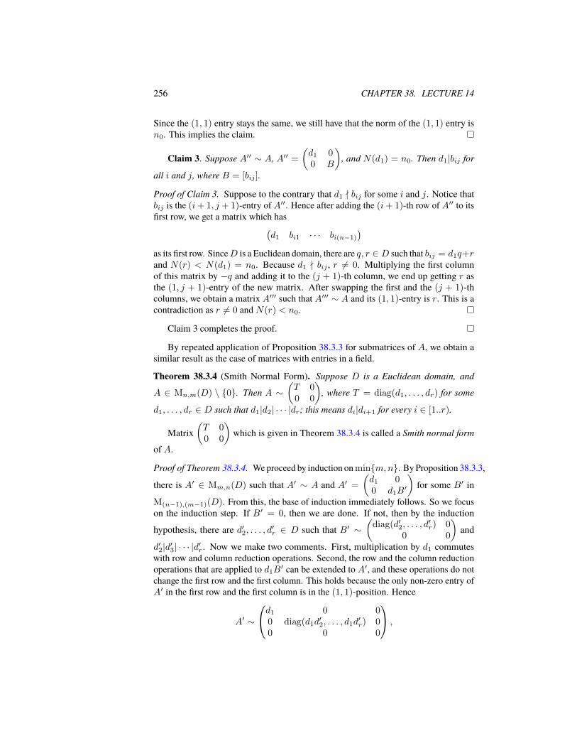
256 CHAPTER 38. LECTURE 14
Since the (1, 1) entry stays the same, we still have that the norm of the (1, 1) entry isn0. This implies the claim.
Claim 3. Suppose A′′ ∼ A, A′′ =
(d1 00 B
), and N(d1) = n0. Then d1|bij for
all i and j, where B = [bij ].
Proof of Claim 3. Suppose to the contrary that d1 - bij for some i and j. Notice thatbij is the (i+ 1, j + 1)-entry of A′′. Hence after adding the (i+ 1)-th row of A′′ to itsfirst row, we get a matrix which has(
d1 bi1 · · · bi(n−1)
)as its first row. SinceD is a Euclidean domain, there are q, r ∈ D such that bij = d1q+rand N(r) < N(d1) = n0. Because d1 - bij , r 6= 0. Multiplying the first columnof this matrix by −q and adding it to the (j + 1)-th column, we end up getting r asthe (1, j + 1)-entry of the new matrix. After swapping the first and the (j + 1)-thcolumns, we obtain a matrix A′′′ such that A′′′ ∼ A and its (1, 1)-entry is r. This is acontradiction as r 6= 0 and N(r) < n0.
Claim 3 completes the proof.
By repeated application of Proposition 38.3.3 for submatrices of A, we obtain asimilar result as the case of matrices with entries in a field.
Theorem 38.3.4 (Smith Normal Form). Suppose D is a Euclidean domain, and
A ∈ Mn,m(D) \ {0}. Then A ∼(T 00 0
), where T = diag(d1, . . . , dr) for some
d1, . . . , dr ∈ D such that d1|d2| · · · |dr; this means di|di+1 for every i ∈ [1..r).
Matrix(T 00 0
)which is given in Theorem 38.3.4 is called a Smith normal form
of A.
Proof of Theorem 38.3.4. We proceed by induction on min{m,n}. By Proposition 38.3.3,
there is A′ ∈ Mm,n(D) such that A′ ∼ A and A′ =
(d1 00 d1B
′
)for some B′ in
M(n−1),(m−1)(D). From this, the base of induction immediately follows. So we focuson the induction step. If B′ = 0, then we are done. If not, then by the induction
hypothesis, there are d′2, . . . , d′r ∈ D such that B′ ∼(
diag(d′2, . . . , d′r) 0
0 0
)and
d′2|d′3| · · · |d′r. Now we make two comments. First, multiplication by d1 commuteswith row and column reduction operations. Second, the row and the column reductionoperations that are applied to d1B
′ can be extended to A′, and these operations do notchange the first row and the first column. This holds because the only non-zero entry ofA′ in the first row and the first column is in the (1, 1)-position. Hence
A′ ∼
d1 0 00 diag(d1d
′2, . . . , d1d
′r) 0
0 0 0
,
38.3. REDUCED ROW/COLUMN OPERATIONS, SMITH NORMAL FORM. 257
and so d1, d2 = d1d′2, . . . , dr := d1d
′r satisfy the desired properties. This completes
the proof.

Chapter 39
Lecture 15
In this section, first we give a classification of finitely generated modules over aEuclidean domain. This will be done using the fact that every finitely generated moduleover a Noetherian ring is isomorphic to the cokernel of a matrix (see Proposition 38.2.2)and existence of a Smith normal form over Euclidean domains (see Theorem 38.3.4).Next using this classification, we obtain a classification of finitely generated and finiteabelian groups. Finally we further study linear transformations (over a field), and pointout their connections with ring and module theory. Later these connections will beexploited to prove the existence of a rational canonical form of a matrix.
39.1 Finitely generated modules over a Euclidean Domain
By Proposition 38.2.2, we know that every finitely generated module over a Noethe-rian ring is isomorphic to the cokernel of a matrix. The next lemma shows that applyingrow and column reduction operations do not change the cokernel of a matrix up toan isomorphism. This result will enable us to use a Smith normal form to study thecokernel of a matrix over a Euclidean domain.
Lemma 39.1.1. Suppose R is a unital commutative ring and A,A′ ∈ Mn,m(R).Suppose there are U ∈ GLn(R) and V ∈ GLm(R) such that A′ = UAV . ThenCoker(A) ' Coker(A′). In particular, if A ∼ A′, then Coker(A) ' Coker(A′)(recall that ∼ means that A′ can be obtained from A by a series of row and columnreduction operations; see Lemma 38.3.2)
Proof. Note that ImA′ = A′Rm = UAV Rm. Since V is invertible, V Rm = Rm.Hence
ImA′ = UARm = U ImA. (39.1)
Because U is invertible, `U : Rn → Rn, `U (x) := Ux is an R-module isomorphism.Let f : Rn → CokerA′, f(x) := `U (x)+ImA′. Since f is the composite of two sur-jectiveR-module homomorphisms `U and the natural quotient mapRn → Rn/ Im(A′),it is surjective. Notice that x ∈ ker f exactly when `U (x) ∈ ImA′. Hence by (39.1),we obtain that the kernel of f is ImA. Therefore by the first isomorphism theorem,Rn/ ImA ' CokerA′. This means CokerA ' CokerA.
259
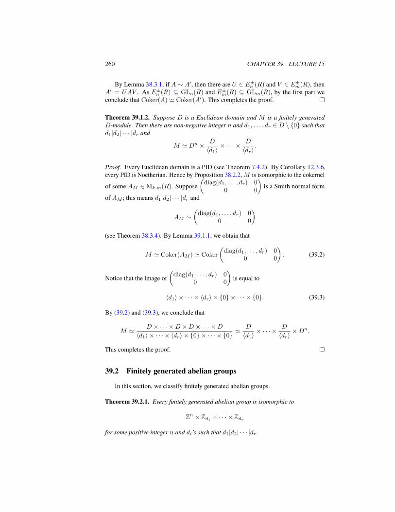
260 CHAPTER 39. LECTURE 15
By Lemma 38.3.1, if A ∼ A′, then there are U ∈ E±n (R) and V ∈ E±m(R), thenA′ = UAV . As E±n (R) ⊆ GLn(R) and E±m(R) ⊆ GLm(R), by the first part weconclude that Coker(A) ' Coker(A′). This completes the proof.
Theorem 39.1.2. Suppose D is a Euclidean domain and M is a finitely generatedD-module. Then there are non-negative integer n and d1, . . . , dr ∈ D \ {0} such thatd1|d2| · · · |dr and
M ' Dn × D
〈d1〉× · · · × D
〈dr〉.
Proof. Every Euclidean domain is a PID (see Theorem 7.4.2). By Corollary 12.3.6,every PID is Noetherian. Hence by Proposition 38.2.2,M is isomorphic to the cokernel
of some AM ∈ Mk,m(R). Suppose(
diag(d1, . . . , dr) 00 0
)is a Smith normal form
of AM ; this means d1|d2| · · · |dr and
AM ∼(
diag(d1, . . . , dr) 00 0
)(see Theorem 38.3.4). By Lemma 39.1.1, we obtain that
M ' Coker(AM ) ' Coker
(diag(d1, . . . , dr) 0
0 0
). (39.2)
Notice that the image of(
diag(d1, . . . , dr) 00 0
)is equal to
〈d1〉 × · · · × 〈dr〉 × {0} × · · · × {0}. (39.3)
By (39.2) and (39.3), we conclude that
M ' D × · · · ×D ×D × · · · ×D〈d1〉 × · · · × 〈dr〉 × {0} × · · · × {0}
' D
〈d1〉× · · · × D
〈dr〉×Dn.
This completes the proof.
39.2 Finitely generated abelian groups
In this section, we classify finitely generated abelian groups.
Theorem 39.2.1. Every finitely generated abelian group is isomorphic to
Zn × Zd1 × · · · × Zdr
for some positive integer n and di’s such that d1|d2| · · · |dr.

39.3. LINEAR TRANSFORMATIONS AND MATRICES 261
Proof. Every finitely generated abelian group A is a finitely generated Z-module.Since Z is a Euclidean domain, by Theorem 39.1.2 there are non-negative integer nand d1, . . . , dr ∈ Z \ {0} such that d1|cdots|dr and
A ' Zn × Z〈d1〉
× · · · × Z〈dr〉
. (39.4)
Since 〈di〉 = 〈−di〉 for every i, without loss of generality we can and will assume thatdi’s are positive integers. Hence A ' Zn × Zd1 × · · · × Zdr as abelian groups. Thiscompletes the proof.
Corollary 39.2.2 (Classification of finite abelian groups). SupposeA is a finite abeliangroup. Then A ' Zd1 × · · · × Zdr for some positive integers di’s such that d1| · · · |dr.
Proof. By Theorem 39.2.1,
A ' Zn × Zd1 × · · · × Zdr
for some positive integer n and di’s such that d1|d2| · · · |dr. Since A is finite, weconclude that n = 0. This completes the proof.
39.3 Linear transformations and matrices
In this section, we discuss the connection between linear transformations andmatrices. Having an arsenal of results from ring and module theory in our disposal,we will prove the existence of a rational canonical from, the Cayley-Hamilton theorem,and further connections between the minimal and the characteristic polynomials of alinear transformation.
Suppose F is a field and V is a finite dimensional vector space over F . For a givenF -basis B := (v1, . . . , vn) of V , we get an F -isomorphism between V and the setMn,1(F ) of column vectors. Hence
`B : Mn,1(F )→ V, `B
c1...cn
:=
n∑i=1
civi
is an F -isomorphism. For every v ∈ V , we let [v]B := `−1B (v). This means
[v]B =
c1...cn
if v = c1v1 + · · ·+ cnvn.
Notice that[vi]B = ei, (39.5)
where ei is an n-by-1 column vector with 1 in its i-th component and zero in everyother. Sometimes we simply write Fn instead of Mn,1(F ).

262 CHAPTER 39. LECTURE 15
Suppose T : V → V is an F -linear transformation. Then T (vi)’s uniquely deter-mine T as we have
T (v) =
n∑i=1
ciT (vi), where
c1...cn
= [v]B.
Hence T is uniquely determined by n column vectors [T (v1)]B, . . . , [T (vn)]B. Weput these column vectors together and get an n-by-nmatrix and denote it by [T ]B. Thismeans
[T ]B = [tij ] if T (vj) = t1jv1 + · · ·+ tnjvj for every j ∈ [1..n].
Since the j-th column of [T ]B is [T (vj)]B, we have [T (vj)]B = [T ]Bej , and so by(39.5), we obtain that
[T (vj)]B = [T ]B[vj ]B. (39.6)
From (39.6), we conclude that for every ci’s in F , we have
[T (
n∑j=1
cjvj)]B =[
n∑j=1
cjT (vj)]B =
n∑j=1
cj [T (vj)]B
=
n∑j=1
cj [T ]B[vj ]B = [T ]B[
n∑j=1
civi]B. (39.7)
By (39.7), we deduce that[T (v)]B = [T ]B[v]B
for every v ∈ V . This is equivalent to saying that the following is a commutativediagram.
V V
Fn Fn
T
[·]B [·]B
[T ]B×
where the bottom row means multiplication by [T ]B, i.e. x 7→ [T ]Bx. We call [T ]Bthe matrix representation of T with respect to the basis B.
From encoding point of view, the more sparse the matrix representation [T ]Bis the better. Here by sparse, we mean having many zero entries. A sparse matrixrepresentation can help us from both computational and theoretical point of view. Laterwe will come back to the problem of finding a sparse matrix representation of a lineartransformation. For now we want to understand the connection between different matrixrepresentations of a given linear transformation.
Suppose B := (v1, . . . , vn) and B′ := (v′1, . . . , v′n) are two F -bases of V . Since
vi’s are linearly independent, there is anF -linear map S : V → V such that S(vi) := v′ifor every i. Because the F -span of v′i’s is V , S is surjective. As v′i’s are F -linearly

39.3. LINEAR TRANSFORMATIONS AND MATRICES 263
independent, S is injective. Hence S : V → V is an isomorphism. Moreover since[vi]B = [v′i]B = ei for every i, we have that the following is a commutative diagram.
V V
Fn Fn
S
[·]B [·]′B
id
This means we have[S(v)]B′ = [v]B (39.8)
for every v ∈ V . Therefore [S]B′ [v]B′ = [v]B for all v ∈ V .For every linear transformation T : V → V , the following is a commutative
diagram.
Fn Fn
V V
Fn Fn
[T ]B′×
[S]B′× [S]B′×T
[·]B
[·]B′
[·]B
[·]B′
[T ]B×
Hence [T ]B′ = [S]−1B′ [T ]B[S]B′ . This means every two matrix representations of a
given linear transformation are conjugate of each other.Conversely, we show that every conjugate of [T ]B is a matrix representation of T .
Suppose S := [sij ] ∈ GLn(F ), and let v′j :=∑ni=1 sijvj . Then B′ := (v′1, . . . , v
′n)
is an F -basis of V , and[v′j ]B = S[v′j ]B′
for every j. Hence [v]B = S[v]B′ for all v ∈ V . Thus by the above discussion,[T ]B′ = S−1[T ]BS, and the converse follows.
Therefore the task of finding a simple matrix representation can be interpreted as asearch for a sparse conjugate of a matrix.
A linear transformation T : V → V is also called an F -endomorphism of V , andthe set of all endormorphisms of V is denoted by EndF (V ). The following lemmashows that EndF (V ) is a ring which is isomorphic to Mn(F ).
Lemma 39.3.1. Suppose F is a field and V is a vector space over F . Suppose B :=(v1, . . . , vn) is an F -basis of V . Then
EndF (V )→ Mn(F ), T 7→ [T ]B
is a bijection, and its inverse is given by
Mn(F )→ EndF (V ), A 7→ λA,
where λA(v) := `B(A[v]B). Moreover, for every T1, T2 ∈ EndF (V ), we have
[T1 + T2]B = [T1]B + [T2]B and [T1 ◦ T2]B = [T1]B[T2]B.
In particular, (EndF (V ),+, ◦) is a ring and it is isomorphic to Mn(F ).

264 CHAPTER 39. LECTURE 15
Proof. Since `B, multiplication byA, and [·]B are F -linear, λA ∈ EndF (V ). Because`B and [·]B are inverse of each other, for all A ∈ Mn(F ) and v ∈ V , we have
[λA]B[v]B = [λA(v)]B = A[v]B.
Hence [λA]B = A.Similarly for all T ∈ EndF (V ) and v ∈ V , we obtain
[λ[T ]B(v)]B = [T ]B[v]B = [T (v)]B,
which implies that λ[T ]B(v) = T (v) for all v ∈ V . Hence λ[T ]B = T . Altogether, weconclude that T 7→ [T ]B is a bijection and A 7→ λA is its inverse.
For every v ∈ V , we have
[T1 + T2]B[v]B =[(T1 + T2)(v)]B = [T1(v) + T2(v)]B
=[T1(v)]B + [T2(v)]B = [T1]B[v]B + [T2]B[v]B
=([T1]B + [T2]B)[v]B,
and so [T1 + T2]B = [T1]B + [T2]B. Similarly we have
[T1 ◦ T2]B[v]B =[(T1 ◦ T2)(v)]B = [T1(T2(v))]B
=[T1]B[T2(v)]B = [T1]B([T2]B[v]B)
=([T1]B[T2]B)[v]B,
which implies that [T1 ◦ T2]B = [T1]B[T2]B.The rest of the claims immediately follow.
39.4 Linear maps, evaluation map, and minimal polynomial
In the study of zeros of polynomials, we saw the importance of evaluation maps. Inthis section, we employ a similar idea to study linear transformations.
Suppose T ∈ EndF (V ), and let φT : F [x]→ EndF (V ), φT (f) := f(T ) be theevaluation at T map. Since scalar transformations are in the center of EndF (V ), thesame argument as in the proof of Lemma 3.1.1 implies that φT is a ring homomorphism.The image of φT is denoted by F [T ]. Notice that F [T ] is a commutative subring ofEndF (V ) which is isomorphic to F [x]/ kerφT .
Notice that by Lemma 39.3.1, we have dimF EndF (V ) = dimF Mn(F ) = n2.Hence dimF F [T ] ≤ n2 < ∞. Therefore dimF ( F [x]
kerφT) < ∞, which implies that
kerφT 6= 0. Because scalar endomorphisms are in F [T ], dimF F [T ] ≥ 1. ThuskerφT is a proper ideal. Since F [x] is a PID and kerφT is a proper non-zero ideal,there is a unique monic non-constant polynomial mT,F ∈ F [x] such that
kerφT = 〈mT,F 〉.
The polynomial mT,F is called the minimal polynomial of T . Altogether we haveproved the following.

39.4. LINEAR MAPS, EVALUATION MAP, AND MINIMAL POLYNOMIAL 265
Lemma 39.4.1. Suppose F is a field and V is a finite dimensional F -vector space.For an F -linear map T : V → V , there is a unique non-constant monic polynomialmT,F ∈ F [x] such that for every p(x) ∈ F [x], we have p(T ) = 0 if and only ifmT,F (x)|p(x).
For a given basis B := (v1, . . . , vn), by Lemma 39.3.1, Mn(F )→ EndF (V )A 7→λA is a ring isomorphism. LetmA,F (x) := mλA,F (x) and call it a minimal polynomialof A. A priori it is not clear why mA,T does not depend on the choice of basis in thedefinition of A 7→ λA. The next lemma, however, shows that mA,F only depends on A.
Lemma 39.4.2. SupposeA ∈ Mn(F ), and let φA : F [x]→ Mn(F ), φA(f) := f(A).Then the following statements hold.
1. The minimal polynomial mA,F is the unique monic generator of kerφA; inparticular, it only depends on A.
2. The image F [A] of φA is isomorphic to F [λA] where λA ∈ EndF (Fn) is givenby λA(x) := Ax.
3. If S ∈ GLn(F ), then mS−1AS,F = mA,F .
Proof. 1. Since Mn(F ) → EndF (Fn), A 7→ λA is a ring isomorphism, for everyf ∈ F [x] we have
λf(A) = f(λA).
Hence f ∈ kerφA if and only if f ∈ kerφλA . Part 1 follows.2. By the first isomorphism theorem, F [A] ' F [x]/ kerφA. By part 1, kerφA =
kerφλA , and so by another application of the first isomorphism theorem we concludethat
F [x]/ kerφA = F [x]/ kerφλA ' F [λA].
This implies the second part.3. Since both A and S−1AS are matrix representations of λA, we deduce that
mA,F = mλA,F = mS−1AS,F ,
which completes the proof.


Chapter 40
Lecture 16
In this section, we use the classification of finitely generated modules over a Eu-clidean domain to find a fairly sparse matrix representation called a rational canonicalform of a linear transformation T : V → V where V is a finite dimensional vectorspace over F . Along the way, we also prove the Cayley-Hamilton theorem and otherproperties of the characteristic and minimal polynomials of T .
40.1 Linear maps, evaluation map, module structure
As we have seen in Section 39.4, for a given linear transformation T : V →V , we can consider the evaluation map φT : F [x] → EndF (V ), and φT is a ringhomomorphism. Via the ring homomorphism φT , we can view V as an F [x]-module.Here is a precise formulation of this result.
Lemma 40.1.1. Suppose F is a field and V is a finite dimensional vector space overF . Let T : V → V is an F -linear map. For f ∈ F [x] and v ∈ V , let
f · v := φT (f)v = f(T )(v). (40.1)
Then V is an F [x]-module with respect to the scalar multiplication given by (40.1)
Proof. It is straightforward to check that the scalar multiplication given in (40.1) sat-isfies all the properties of modules. Here we go through only one of the distributionproperties. Suppose f1, f2 ∈ F [x] and v ∈ V . Then
(f1 + f2) · v =φT (f1 + f2)(v) = (φT (f1) + φT (f2))(v)
=φT (f1)(v) + φT (f2)(v) = f1 · v + f2 · v.
Notice that F [x]-module structure of V and its F -vector space structure are com-patible. This is the case because constant polynomials are sent to scalar linear trans-formations: for every c ∈ F and v ∈ V , we have φT (c)(v) = cv where cv is thescalar product of c by v as an F -vector space. By this remark, we deduce that, if
267
268 CHAPTER 40. LECTURE 16
B = (v1, . . . , vn) is an F -basis of V , then vi’s generate V as an F [x]-module as well.Hence V is a finitely generated F [x]-module. Since F [x] is a Euclidean domain, byTheorem 39.1.2 there are a non-negative integer k and d1, . . . , dr ∈ F [x] \ {0} suchthat
V ' F [x]k × F [x]
〈d1〉× · · · × F [x]
〈dr〉(40.2)
as an F [x]-module and d1| · · · |dr. Since V is a finite dimensional vector space overF and F [x] is an infinite dimensional vector space over F , by (40.2) we conclude thatk = 0. Thus
V ' F [x]
〈d1〉× · · · × F [x]
〈dr〉. (40.3)
Notice that if di is a non-zero constant, then 〈di〉 = F [x] and F [x]〈di〉 = 0, and so such a
factor can be dropped. Let’s also observed that multiplying di’s by a non-zero constantdoes not change the ideals 〈di〉’s. Hence without loss of generality we can and willassume that di’s are monic non-constant polynomials. Let’s summarize what we haveobtained so far.
Lemma 40.1.2. Suppose F is a field and V is a finite dimensional F -vector space.Suppose T : V → V is anF -linear map. Then V can be viewed as anF [x]-module withthe scalar multiplication given in (40.1), and there are non-constant monic polynomialsd1, . . . , dr ∈ F [x] such that d1| · · · |dr and
V ' F [x]
〈d1〉× · · · × F [x]
〈dr〉.
40.2 Reduction to the cyclic case.
In this section, we see how the module structure of V given in Lemma 40.1.2 canhelp us get a matrix representation of T that is of block form and its non-zero blockscan only be on the diagonal. Moreover the associated blocks are related to the casewhere the vector space is isomorphic to F [x]/〈d〉 for some d as an F [x]-module. Noticethat by Lemma 37.3.2, an F [x]-module is isomorphic to F [x]/〈d〉 exactly when it is acyclic F [x]-module. Altogether, we are reducing the problem of finding a sparse matrixrepresentation of T to the case where V is a cyclic F [x]-module.
Suppose di’s are given as in Lemma 40.1.2, and
θ :F [x]
〈d1〉× · · · × F [x]
〈dr〉→ V
is an F [x]-module isomorphism. Let M := F [x]〈d1〉 × · · · ×
F [x]〈dr〉 . Then for all m ∈ M
we haveT (θ(m)) = x · θ(m) = θ(x ·m).

40.3. CYCLIC CASE, COMPANION MATRIX, AND RATIONAL CANONICAL FORM269
This means that the following is a commutative diagram.
M M
V V
x×
θ θ
T
Hence if B := (m1, . . . ,mn) is an F -basis of M , then θ(B) := (θ(m1), . . . , θ(mn))is an F -basis of V and [x×]B = [T ]θ(B). Roughly this diagram implies that afteridentifying M with V , x× gets identified with T . Hence x× and T share matrixrepresentations. Here is a more formal argument of why the last equality holds: suppose[x×]B = [rij ]. Then x · mj =
∑ni=1 rijmi for all j. As θ is an F [x]-module
homomorphism, we obtain that θ(x ·mj) = x · θ(mj) = T (θ(mj)). Therefore
T (θ(mj)) = θ(x ·mj) = θ(
n∑i=1
rijmi) =
n∑i=1
rijθ(mi),
which implies that [T ]θ(B) = [rij ].Since every matrix representation of x× is a matrix representation of T (and vice
versa), we will find a sparse matrix representation of x×.LetMi := 0×· · ·× F [x]
〈di〉 ×· · ·× 0 for all i. Notice thatMi’s are F [x]-submodulesof M , M = M1 + · · ·+Mr, and if vi ∈Mi \ {0}, then vi’s are linearly independent.Hence if Bi is an F -basis of Mi, then B := B1 ∪ · · · ∪Br (with this ordering) isan F -basis of M . Because Mi is an F [x]-submodule, for every m ∈ Bi the elementx ·m is an F -linear combination of elements of Bi. Hence [x×]B is a matrix of thefollowing form:
[x×]B1 0 · 00 [x×]B2
· · · 0...
.... . .
...0 0 · · · [x×]Br
(40.4)
Thus to make this matrix representation more sparse, we should focus on x× for acyclic F [x]-module of the form F [x]/〈d〉 where d is a non-constant monic polynomial.
40.3 Cyclic case, companion matrix, and rational canonical form
In this section, we find a nice matrix representation of x× for a cyclic F [x]-moduleof the form F [x]/〈d(x)〉 where d(x) := xm + am−1x
m−1 + · · · + a0 ∈ F [x]. Wealso find its minimal polynomial.
By Proposition 20.1.1, B := (1, x, . . . , xm−1) is an F -basis of F [x]〈d(x)〉 where xi =
xi + 〈d〉 for every non-negative integer i. Notice that
1x×7−−→ x
x×7−−→ x2 x×7−−→ · · · x×7−−→ xm−1 x×7−−→ xm. (40.5)
For every i ∈ [0..(m− 1)], we have [xi]B = ei+1 where (e1, . . . , em) is the standardbasis of Fm. We also notice that
xm + am−1xm−1 + · · ·+ a0 = 0

270 CHAPTER 40. LECTURE 16
which implies that
[xm]B =[−m−1∑i=0
aixi]B
=
m−1∑i=0
(−ai)ei+1 =
−a0
...−am−1
. (40.6)
By (40.5) and (40.6), we obtain that
[x×]B =
0 0 0 · · · 0 −a0
1 0 0 · · · 0 −a1
0 1 0 · · · 0 −a2
......
......
...0 0 0 · · · 0 −am−2
0 0 0 · · · 1 −am−1
. (40.7)
Let C(d) be the matrix given in (40.7). We call C(d) the companion matrix of themonic polynomial d(x) = xm + am−1x
m−1 + · · ·+ a0.To find the minimal polynomial of x× : F [x]
〈d〉 →F [x]〈d〉 , we need to find the kernel
of the evaluation map φx×. Notice that (x×)i = xi× for every non-negative integer i.Hence for every polynomial f(x) ∈ F [x], we have φx×(f) = f(x)×. This means forevery g + 〈d〉 ∈ F [x]
〈d〉 , we have
φx×(f)(g + 〈d〉) = f(x)g(x) + 〈d〉.
Hence f ∈ kerφx× if and only if d|fg for every g ∈ F [x]. Hence kerφx× = 〈d〉.Because d is a monic polynomial which generates kerφx×, we conclude that theminimal polynomial of x× is d. Therefore we obtain the following result.
Lemma 40.3.1. Suppose d ∈ F [x] is a monic non-constant polynomial. Then theminimal polynomial of the companion matrix C(d) is d(x).
By (40.4) and (40.7), we obtain the following result.
Theorem 40.3.2 (Rational canonical form). Suppose V is a finite dimensional vectorspace over a field F , and T : V → V is an F -linear map. Then T has a matrixrepresentation of the form C(d1) · · · 0
.... . .
...0 · · · C(dr)
(40.8)
for some monic non-constant polynomials di’s in F [x] such that d1| · · · |dr.
The matrix given in (40.8) is called a rational canonical form of T .

40.4. THE CAYLEY-HAMILTON THEOREM 271
40.4 The Cayley-Hamilton Theorem
In this section, we define the characteristic polynomial of a linear map, give aconnection with a rational canonical form of a linear map, and prove the Cayley-Hamilton Theorem.
Definition 40.4.1. Suppose R is a unital commutative ring and A ∈ Mn(R). Thecharacteristic polynomial of A is fA(x) := det(xI −A) where xI −A ∈ Mn(R[x]).Suppose F is a field, V is a finite dimensional vector space over F , and B is an F -basisof V . The characteristic polynomial of an F -linear map T : V → V with respect tothe basis B is f[T ]B(x). 1
Lemma 40.4.2. Suppose R is a unital commutative ring, F is a field and V is a finitedimensional vector space over F .
1. If A,A′ ∈ Mn(R) are conjugate of each other, then fA(x) = fA′(x).
2. If B and B′ are two F -bases of V , then the characteristic polynomials of T withrespect to B and B′ are the same.
Proof. (1) Since A and A′ are conjugate of each other, there is S ∈ GLn(R) such thatA′ = SAS−1. Because determinant is multiplicative we have
det(A′) = det(SAS−1) = det(S) det(A) det(S−1)
= det(S) det(S−1) det(A) = det(SS−1) det(A)
= det(I) det(A) = det(A).
(2) Since [T ]B and [T ]B′ are conjugate of each other, by part (1), f[T ]B = f[T ]B′. This
completes the proof.
By the second part of Lemma 40.4.2, we deduce that the characteristic polynomialof a linear map does not depend on the choice of a basis of the vector space. Thecharacteristic polynomial of a linear map T : V → V is denoted by fT .
Lemma 40.4.3. Suppose d(x) ∈ F [x] is a monic polynomial and C(d) is its thecompanion matrix. Then the characteristic polynomial of C(d) is d.
Proof. We proceed by induction on the degree of d. If deg d = 1, then d(x) = x+ aand C(d) = [−a]. So fC(d)(x) = det([x+ a]) = x+ a. Next we prove the induction
1Look at the HW assignment week 8 for the definition and properties of determinant.

272 CHAPTER 40. LECTURE 16
step. We expand the determinant of xI − C(d) with respect to the first column. Hence
det
x 0 · · · a0
−1 x · · · a1
......
...0 0 · · · x+ am−1
=xdet
x 0 · · · a1
−1 x · · · a2
......
...0 0 · · · x+ am−1
+ det
0 0 · · · a0
−1 x · · · a2
......
...0 0 · · · x+ am−1
We use the induction hypothesis for the first term, and expand the determinant of thesecond term with respect to the first row. We obtain the following.
fC(d)(x) =x(xm−1 + am−1xm−2 + · · ·+ a1)
+(−1)1+(m−1)a0 det
−1 x · · · 00 −1 · · · 0...
......
0 0 · · · −1
=x(xm−1 + am−1x
m−2 + · · ·+ a1) + (−1)m+m−2a0
=xm + am−1xm−1 + · · ·+ a1x+ a0 = d(x).
This completes the proof.
Theorem 40.4.4. Suppose d1, . . . , dr ∈ F [x] are monic polynomials, d1| · · · |dr, anddiag(C(d1), . . . , C(dr)) is a rational canonical form of a linear map T : V → V .Then following statements hold.
1. mT,F (x) = dr(x).
2. fT (x) = d1(x) · · · dr(x).
3. (Caley-Hamilton Theorem) fT (T ) = 0.
4. Suppose p(x) ∈ F [x] is irreducible. Then p(x)|fT (x) if and only if p(x)|mT,F (x).
Proof. Let A := diag(C(d1), . . . , C(dr)). Then
fT (x) = fA(x) and mT,F (x) = mA,F (x).
For every polynomial f ∈ F [x], we have
f(A) = diag(f(C(d1)), . . . , f(C(dr))).
Hence f(A) = 0 if and only if f(C(di)) = 0 for every i. By Lemma 40.3.1,mC(di),F (x) = di(x). Therefore f(A) = 0 exactly when di(x)|f(x) for all i. Since

40.4. THE CAYLEY-HAMILTON THEOREM 273
d1| · · · |dr, we obtain that f(A) = 0 precisely when dr|f . Thus mA,F (x) = dr(x).Next we want to find the characteristic polynomial of A:
fA(x) = det(diag(xI − C(d1), . . . , xI − C(dr)))
=
r∏i=1
det(xI − C(di)) =
r∏i=1
fC(di)(x) (by Lemma 40.4.3)
=
r∏i=1
di(x).
Since mT,F (x) = dr(x) and fT (x) =∏ri=1 di(x), mT,F (x)|fT (x). Hence
fT (T ) = 0.
Suppose p is an irreducible factor of fT (x). Since fT (x) =∏ri=1 di(x), p|fT , and
p is prime, p divides di for some i. Since di|dr for all i, we conclude that p|dr. AsmT,F (x) = dr(x), we obtain that p|mT,f . This completes the proof.


Chapter 41
Lecture 17
In our study of zeros of multivariable polynomials, we investigated system of linearequations over unital commutative rings. We developed module theory and gave analgorithm for solving system of linear equations over a Euclidean domain. In the nextstep, we consider two related directions to extend our exploration:
1. Studying single variable polynomials over an arbitrary unital commutative ring.
2. Studying multivariable polynomials over a field.
Since F [x1, . . . , xn] is essentially (F [x1, . . . , xn−1])[xn], it is not surprising that anyresult related to the first task has implications towards the second one.
Suppose A is a unital commutative ring. We would like to understand ring theoreticproperties of A[x]. Here are some results that we have proved earlier:
1. If D is an integral domain, then D[x] is an integral domain. (See Lemma 6.3.1)
2. If F is a field, then F [x] is a PID. (See Theorem 7.3.1)
3. If D is a UFD, then D[x] is a UFD. (See Theorem 15.4.4)
One of the key results which is instrumental in proving these results is the longdivision (see Theorem 6.4.1). Let’s recall the long division algorithm.
Suppose A is a unital commutative ring and g ∈ A[x] such that 〈ld(g)〉 = A whereld(g) is the leading coefficient of g. Then for every f ∈ A[x] there is a unique r ∈ A[x]such that f + 〈g〉 = r + 〈g〉 and deg r < deg g.
So the long division algorithm gives us a (canonical) simple coset representative off + 〈g〉 if the leading coefficient of g generates the entire ring of coefficients.
The existence part of the long division is derived from the following algorithm.
Step 1. If deg f < deg g, we are done. Return r := f .
Step 2. If deg f ≥ deg g, there is a monomial cxk such that Ld(f) = Ld(g)(cxk). Letfnew ← fold − (cxk)g.
Here are a few comments about the above algorithm:
275

276 CHAPTER 41. LECTURE 17
1. It terminates as deg fnew is less than deg fold.
2. At every step, we do not leave the coset f + 〈g〉 since fnew + 〈g〉 = fold + 〈g〉.
3. the key reason that it actually works is because Ld(f) ∈ 〈Ld(g)〉 unless deg f isless than deg g.
There are a few ways to generalize long division. But the general idea stays the same:considering a grading on the given ring and clearing the leading term in the process.
41.1 Generalized long division
In this section, we present some generalizations of long division.
Lemma 41.1.1. Suppose A is a unital commutative ring and g1, . . . , gn ∈ A[x] suchthat
〈ld(g1), . . . , ld(gn)〉 = A. (41.1)
Then for every f ∈ A[x], there is r ∈ A[x] such that
f + 〈g1, . . . , gn〉 = r + 〈g1, . . . , gn〉 and deg r < max(deg g1, . . . ,deg gn).
Proof. We follow the same algorithm as in the case when n = 1.
Step 1. If deg f < max(deg g1, . . . ,deg gn), we are done. Return r := f .
Step 2. If deg f ≥ max(deg g1, . . . ,deg gn), then
Ld(f) ∈ 〈Ld(g1), . . . ,Ld(gk)〉. (41.2)
Here is why (41.2) holds. By (41.1)
ld(f) = a1 ld(g1) + · · ·+ an ld(gn)
for some ai’s in A. Therefore we obtain that
Ld(f) = (a1xdeg f−deg g1) Ld(g1) + · · ·+ (anx
deg f−deg gn) Ld(gn). (41.3)
Suppose ai’s are as in (41.3), and let
fnew ← fold − ((a1xdeg f−deg g1)g1 + · · ·+ (anx
deg f−deg gn)gn).
Notice that deg fnew < deg fold and
fnew + 〈g1, . . . , gn〉 = fold + 〈g1, . . . , gn〉.
Hence this algorithm terminates and returns a desired r.
41.1. GENERALIZED LONG DIVISION 277
A closer look at the proof of Lemma 41.1.1 shows that the key properties to haveare
ld(f) ∈ 〈ld(g1), . . . , ld(gn)〉 (41.4)
andLd(f) ∈ 〈Ld(g1), . . . ,Ld(gn)〉. (41.5)
The following results are good examples of how one can use the conditions given in(41.4) and (41.5).
Lemma 41.1.2. SupposeA is a untial commutative ring, IEA[x], and g1, . . . , gn ∈ Iare such that
ld(f) ∈ 〈ld(g1), . . . , ld(gn)〉 (41.6)
for all f ∈ I . Then for every f ∈ I , there is r ∈ I such that
f + 〈g1, . . . , gn〉 = r + 〈g1, . . . , gn〉 and deg r < max(deg g1, . . . ,deg gn).
Lemma 41.1.3. SupposeA is a untial commutative ring, IEA[x], and g1, . . . , gn ∈ Iare such that
Ld(f) ∈ 〈Ld(g1), . . . ,Ld(gn)〉. (41.7)
Then I = 〈g1, . . . , gn〉.
Proof of Lemma 41.1.2. We follow an almost identical line of argument as in the proofof Lemma 41.1.1. Consider the following algorithm:
Step 1. If deg f < max(deg g1, . . . ,deg gn), we are done. Return r := f .
Step 2. If deg f ≥ max(deg g1, . . . ,deg gn), then
Ld(f) ∈ 〈Ld(g1), . . . ,Ld(gk)〉. (41.8)
Here is why (41.8) holds. By (41.6)
ld(f) = a1 ld(g1) + · · ·+ an ld(gn)
for some ai’s in A. Therefore we obtain that
Ld(f) = (a1xdeg f−deg g1) Ld(g1) + · · ·+ (anx
deg f−deg gn) Ld(gn). (41.9)
Suppose ai’s are as in (41.9), and let
fnew ← fold − ((a1xdeg f−deg g1)g1 + · · ·+ (anx
deg f−deg gn)gn).
Notice that deg fnew < deg fold and
fnew + 〈g1, . . . , gn〉 = fold + 〈g1, . . . , gn〉.
Moreover, since fold and gi’s are in I , so is fnew. Hence this algorithm terminates andreturns a desired r.
278 CHAPTER 41. LECTURE 17
Proof of Lemma 41.1.3. Since gi’s are in I , 〈g1, . . . , gn〉 ⊆ I . Next by strong inductionon degree, we show that every f ∈ I is in 〈g1, . . . , gn〉. This will be done essentiallyfollowing a similar generalized long division algorithm. By hypothesis, Ld(f) is in theideal generated by Ld(gi)’s. Hence there are qi’s in A[x] such that
Ld(f) = q1 Ld(g1) + · · ·+ qn Ld(gn). (41.10)
Suppose deg f = m, deg gi = mi, and qi(x) = cixm−mi + qi where qi ∈ A[x] does
not have a monomial of degree (m−mi). Notice that if m < mi, then ci = 0. Thennone of the terms of
q1 Ld(g1) + · · ·+ qn Ld(gn)
is of degree m. Therefore by (41.10), we obtain
Ld(f) = (c1xm−m1) Ld(g1) + · · ·+ (cnx
m−mn) Ld(gn). (41.11)
Letf(x) := f(x)− ((c1x
m−m1)g1 + · · ·+ (cnxm−mn)gn). (41.12)
Then because of (41.11), deg f < deg f . Moreover since f and gi’s are in I , so isf . Hence by the strong induction hypothesis, f ∈ 〈g1, . . . , gn〉. Thus by (41.12), weconclude that f ∈ 〈g1, . . . , gn〉. This completes the proof.
By Lemma 41.1.3, we deduce that to generate an ideal I of A[x], it is enough togenerate all the leading terms. Next we focus more on leading coefficients.
Lemma 41.1.4. Suppose A is a unital commutative ring and I is an ideal of A[x]. Let
ld(I) := {ld(f) | f ∈ I \ {0}} ∪ {0},
andldm(I) := {ld(f) | f ∈ I, deg f = m} ∪ {0}
for every non-negative integer m. Then ld(I) and ldm(I) are ideals of A.
Proof. Suppose c1, c2 ∈ ld(I). Then there are f1, f2 ∈ I such that Ld(fi) = cixmi
for some non-negative integersmi’s. Without loss of generality, we can and will assumethat m1 ≤ m2. Then, if c1 + c2 6= 0, then
Ld(xm2−m1f1 + f2) = (c1 + c2)xm2
Hence c1 +c2 is the leading coefficient of xm2−m1f1 +f2. Notice that xm2−m1f1 +f2
is in I as fi’s are in I . Therefore c1 + c2 is either 0 or it is the leading coefficient of anelement of I . Hence in either case c1 + c2 ∈ ld(I).
For every a ∈ A, either ac1 = 0 or ld(af1) = ac1. In either case, ac1 ∈ ld(I).Altogether, we obtain that ld(I) is an ideal of A.
Next we show that ldm(I) is an ideal. We start by discussing why it is closed underaddition. If c1, c2 ∈ ldm(I), then there are f1, f2 ∈ I such that Ld(fi) = cix
m fori = 1, 2. Hence either c1 + c2 = 0 or Ld(f1 + f2) = (c1 + c2)xm. In either case,c1 + c2 ∈ ldm(I). For a ∈ A, either ac1 = 0 or Ld(af1) = ac1x
m. Therefore ineither case, ac1 ∈ ldm(I). Since ldm(I) is closed under addition and multiplication byelements ofA, we conclude that ldm(I) is an ideal ofA. This completes the proof.
41.2. HILBERT’S BASIS THEOREM 279
41.2 Hilbert’s basis theorem
We have proved many results connecting (generating) an ideal of A[x] with idealsof A. So we are well-placed to prove that if every ideal of A is finitely generated, thenall ideals of A[x] are finitely generated. Recall that all ideals of a ring R are finitelygenerated if and only if R is Noetherian.
Theorem 41.2.1 (Hilbert’s basis theorem). Suppose A is a Noetherian unital commu-tative ring. Then A[x] is Noetherian.
Proof. By Lemma 12.3.5, we know that A[x] is Noetherian if and only if every idealof A[x] is finitely generated. Suppose I is an ideal of A[x]. By Lemma 41.1.3, it isenough to show that there are g1, . . . , gn ∈ I such that for all f ∈ I ,
Ld(f) ∈ 〈Ld(g1), . . . ,Ld(gn)〉.
Let Ld(I) be the ideal generated by Ld(f)’s as f ranges in I .Claim. There are g1, . . . , gn ∈ I such that Ld(I) = 〈Ld(g1), . . . ,Ld(gn)〉.
Proof of Claim. Since A is Noetherian, ld(I) is a finitely generated ideal. Hence thereare f1, . . . , fm ∈ I such that
ld(I) = 〈ld(f1), . . . , ld(fm)〉. (41.13)
By (41.9), if f ∈ I and deg f ≥ max(deg f1, . . . ,deg fm), then
Ld(f) ∈ 〈Ld(f1), . . . ,Ld(fm)〉. (41.14)
Next we want to generate all the leading terms Ld(f) of polynomials f ∈ I with deg fless than k := max(deg f1, . . . ,deg fm). By Lemma 41.1.4, ldi(I)’s are ideals of Afor every integer i in [0, k). Since A is Noetherian, ldi(I) is a finitely generated ideal.Hence for every index i, there are fi1, . . . , fini ∈ I such that deg fij = i for everyindex j and
ldi(I) = 〈ld(fi1), . . . , ld(fini)〉. (41.15)
Next we show that if f ∈ I and deg f = i for some non-negative integer i < k, then
Ld(f) ∈ 〈Ld(fi1), . . . ,Ld(fini)〉. (41.16)
Notice that ld(f) ∈ ldi(f), and so by (41.15), there are a1, . . . , ani ∈ A such that
ld(f) = a1 ld(fi1) + · · ·+ ani ld(fini). (41.17)
Because of (41.17), we conclude that
Ld(f) = ld(f)xi = (a1 ld(fi1) + · · ·+ ani ld(fini))xi
=a1 Ld(fi1) + · · ·+ ani Ld(fini). (41.18)
By (41.18), we deduce that (41.16) holds. By (41.14) and (41.16), we obtain that forall f ∈ I ,
Ld(f) ∈ 〈Ld(fr),Ld(fij) | 1 ≤ r ≤ m, 0 ≤ i < k, 1 ≤ j ≤ ni〉.
280 CHAPTER 41. LECTURE 17
This implies that
Ld(I) = 〈Ld(fr),Ld(fij) | 1 ≤ r ≤ m, 0 ≤ i < k, 1 ≤ j ≤ ni〉
as fr’s and fij’s are in I . This completes the proof of Claim.
By above Claim and Lemma 41.1.3, we conclude that I is a finitely generated ideal.This completes the proof of Hilbert’s basis theorem.
41.3 Finitely generated rings and algebras
Hilbert’s basis theorem implies that many of the rings that we have been workingwith are Noetherian. Here is an immediate corollary of Hilbert’s basis theorem.
Corollary 41.3.1. SupposeA is a Noetherian unital commutative ring. ThenA[x1, . . . , xn]is Noetherian.
Proof. We proceed by induction on n. The case of n = 0 follows from the hypothesis.So we focus on the induction step. By the induction hypothesis, A[x1, . . . , xn] isNoetherian. Hence by Hilbert’s basis theorem, (A[x1, . . . , xn])[xn+1] is Noetherian.This completes the proof.
Corollary 41.3.2. The rings Z[x1, . . . , xn] and F [x1, . . . , xn], where F is a field, areNoetherian.
Proof. This follows from Corollary 41.3.1 and the fact that the ring of integers andfields are Noetherian.
Corollary 41.3.2 implies that every finitely generated ring or finitely generatedF -algebra is Noetherian.
Definition 41.3.3. (1) We say a unital commutative ring A is finitely generated if thereare a1, . . . , an ∈ A such that the smallest subring of A which contains ai’s is A.
(2) Suppose F is field. We say a unital commutative ring A is called a finitelygenerated F -algebra if F is a subring of A, 1F = 1A, and there are a1, . . . , an in Asuch that the smallest subring of A which contains F and ai’s is A. In this case wewrite A = F [a1, . . . , an].
The following easy lemma implies that every finitely generated ring is a quotientof the ring of polynomials Z[x1, . . . , xn] for some positive integer n and every finitelygenerated F -algebra is a quotient of the ring of polynomials F [x1, . . . , xn] for somepositive integer n.
Lemma 41.3.4. 1. Suppose A is generated by a1, . . . , an as a ring. Then the fol-lowing is a surjective homomorphism Z[x1, . . . , xn]→ A,∑
i1,...,in
mi1,...,inxi11 · · ·xinn 7→
∑i1,...,in
e(mi1,...,in)ai11 · · · ainn
where e : Z→ A, e(m) := m1A (see Lemma 2.3.1)

41.3. FINITELY GENERATED RINGS AND ALGEBRAS 281
2. Suppose F is a field and A is a finitely generated F -algebra. Suppose A =F [a1, . . . , an]. Then the evaluation map
φa1,...,an : F [x1, . . . , xn]→ A, φa1,...,an(f) := f(a1, . . . , an)
is a surjective ring homomorphism.
Proof. We leave the proof as an exercise.
We obtain the following important consequence of Hilbert’s basis theorem.
Theorem 41.3.5. Suppose A is either a finitely generated ring or a finitely generatedF -algebra, where F is a field. Then A is Noetherian.
Proof. By Lemma 41.3.4,A is isomorphic to eitherZ[x1, . . . , xn]/I orF [x1, . . . , xn]/Ifor some integer n and ideal I . Since a quotient of a Noetherian ring is Noetherian, byCorollary 41.3.2 we obtain that A is Noetherian. This completes the proof.

Chapter 42
Lectures 18 and 19
In this section, we want to study zeros of multivariable polynomials with coefficientsin a field. As we have mentioned in Section 38.3, a system of linear equations can besolved using the GAuss-Jordan elimination process. In the higher degree setting, wewill use an argument inspired by the elimination process to find one solution of thegiven system of polynomial equations if it has a solution.
42.1 Set of common zeros and vanishing polynomials
In the single variable case, we have seen the importance of viewing polynomials asfunctions and exploring the connection between zeros of polynomials and ideals of ringof polynomials. We start by observing a similar connection in a multivariable setting.
For a subset S of F [x1, . . . , xn], let
Z(S) := {a ∈ Fn | f(a) = 0 for all f ∈ S}.
For a subset V of Fn, let
I(V ) := {f ∈ F [x1, . . . , xn] | f(v) = 0 for all v ∈ V }.
Alternatively we can say that f ∈ I(V ) if and only if the restriction f |V of f to V iszero where we are viewing f as a function from Fn to F . For V ⊆ Fn, let Fun(V, F )be the set of functions from V to F . Then it is easy to see that Fun(V, F ) is a ring withrespect to pointwise addition and multiplication; that means (f + g)(x) = f(x) + g(x)and (f ·g)(x) := f(x)g(x) for every x ∈ V . By means of evaluation, we get a function
F [x1, . . . , xn]→ Fun(V, F ), f 7→ f |V . (42.1)
It is easy to see that this is a ring homomorphism. From the definition I(V ), we havethat I(V ) is the kernel of the ring homomorphism given in (42.1). The next lemmagives us basic properties of Z and I .
Lemma 42.1.1. Suppose F is a field.
283
284 CHAPTER 42. LECTURES 18 AND 19
1. Functions I and Z are inclusion-reversing. That means for every V1 ⊆ V2 ⊆ Fn,I(V2) ⊆ I(V1), and for every S1 ⊆ S2 ⊆ F [x1, . . . , xn], Z(S2) ⊆ Z(S1).
2. For every V ⊆ Fn, I(V ) is an ideal of F [x1, . . . , xn], and V ⊆ Z(I(V )).
3. For every S ⊆ F [x1, . . . , xn], 〈D〉 ⊆ I(Z(S)).
4. For every S ⊆ F [x1, . . . , xn], Z(S) = Z(〈S〉) and there are finitely manypolynomials g1, . . . , gm such that
Z(S) = Z({g1, . . . , gm}).
Proof. (1) If f ∈ I(V2), then f |V2 = 0. Since V1 ⊆ V2, we conclude that f |V1 = 0.Therefore f ∈ I(V1). This shows that I(V2) ⊆ I(V1).
Suppose v ∈ Z(S2). Then for every f ∈ S2, f(v) = 0. As S1 ⊆ S2, for everyf ∈ S1 we have f(v) = 0. Hence v ∈ Z(S1). This means Z(S2) ⊆ Z(S2).
(2) For all v ∈ V and f ∈ I(V ), f(v) = 0. Hence v is a common zero of elementsof I(V ). This means v ∈ Z(I(V )). Hence V ⊆ Z(I(V )).
We have already mentioned that I(V ) is the kernel of the ring homomorphism
F [x1, . . . , xn]→ Fun(V, F ), f 7→ f |V .
Hence I(V ) is an ideal.(3) For all f ∈ S and v ∈ Z(S), f(v) = 0. Hence f |Z(S) = 0. Therefore
S ⊆ I(Z(S)). Because I(Z(S)) is an ideal, we obtain that 〈S〉I(Z(S)).(4) Since 〈S〉 ⊆ I(Z(S)), for all v ∈ Z(S) and f ∈ 〈S〉 we have f(v) = 0.
Hence v ∈ Z(〈S〉). Hence Z(S) ⊆ Z(〈S〉). Because Z is an order-reversing map andS ⊆ 〈S〉, we conclude that Z(〈S〉) ⊆ Z(S). Altogether, we obtain that
Z(S) = Z(〈S〉).
Finally by Hilbert’s basis theorem, every ideal of F [x1, . . . , xn] is finitely generated.Therefore there are g1, . . . , gn ∈ F [x1, . . . , xn] such that 〈S〉 = 〈g1, . . . , gn〉. Hence
Z(S) = Z(〈S〉) = Z(〈g1, . . . , gn〉) = Z({g1, . . . , gn}).
This completes the proof.
42.2 Our general approach for finding a solution
Solving a system of polynomial equations
g1(x1, . . . , xn) =0
... (42.2)gm(x1, . . . , xn) =0
is the same as understanding Z(I) where I is the ideal generated by gi’s. As wementioned earlier, we use an approach inspired by the elimination process to find oneelement of Z(I) if possible. Eliminating variable xn roughly means:

42.2. OUR GENERAL APPROACH FOR FINDING A SOLUTION 285
1. Deriving equations from (42.2) where xn does not appear.
2. Finding xn in terms of x1, . . . , xn−1.
Notice that the first item essentially means considering I ∩ F [x1, . . . , xn−1]. Next fora given
(a1, . . . , an−1) ∈ Z(I ∩ F [x1, . . . , xn−1]),
we have to find xn = an which satisfies (42.2). This can be interpreted as follows.Consider the projection
π : Z(I)→ Z(I ∩ F [x1, . . . , xn−1]), π(α1, . . . , αn) := (α1, . . . , αn−1).
The above approach suggests that π is a surjective map; finding a point (a1, . . . , an−1)in the codomain, we look for (a1, . . . , an) in the preimage π−1 of (a1, . . . , an−1). Ingeneral, it is, however, not true that π is surjective. To avoid this problem, instead ofprojecting to a standard (n − 1)-dimensional subspace, we will carefully choose aprojection to an (n− 1)-dimensional subspace. To find out, how the needed projectioncan be chosen, we start with the standard projection π and find out when π is notsurjective. Next we make a linear change of coordinates to avoid the bad cases, andmake sure that π is surjective.
We also notice that one cannot expect that even a single variable polynomial to havea zero in F unless F is algebraically closed. So we will be assuming that the followingholds:
Our standing assumption. Suppose F is an algebraically closed field and I is anideal of F [x1, . . . , xn]. Suppose a := (a1, . . . , an−1) is in Z(I ∩ F [x1, . . . , xn−1])and π−1(a) = ∅ where
π : Z(I)→ Z(I ∩ F [x1, . . . , xn−1]), π(α1, . . . , αn) := (α1, . . . , αn−1).
Notice that π−1(a) = ∅ if and only if Z(φa(I)) = ∅ where
φa(f) = f(a1, . . . , an−1, xn) ∈ F [xn].
Since the map φa of evaluation at a is surjective, φa(I) is an ideal of F [xn]. BecauseF [xn] is a PID, φa(I) = 〈pa(xn)〉 for some polynomial pa(xn) ∈ F [xn]. HenceZ(φa(I)) is the same as the set of zeros of pa(xn) in F . Since F is algebraicallyclosed, every non-unit polynomial F [xn] has a zero in F . Therefore Z(φa(I)) = ∅exactly when pa(xn) is a non-zero constant polynomial. Thus φa(I) = ∅ preciselywhen 1 ∈ φa(I). Hence our standing assumption implies that there is f ∈ I such thatφa(f) = 1. Let A := F [x1, . . . , xn−1], view F [x1, . . . , xn] as A[xn], and write
f := fdxdn + · · ·+ f1xn + f0
for some fi’s in A. Then φa(f) = 1 implies that
1 = fd(a)xdn + · · ·+ f1(a)xn + f0(a).
286 CHAPTER 42. LECTURES 18 AND 19
Hence we obtain
fd(a) = fd−1(a) = · · · = f1(a) = 0, and f0(a) = 1. (42.3)
For every g ∈ I , we will look for elements of the form rf +sg inA where r, s ∈ A[xn].Notice that for every such element, we have rf + sg ∈ I ∩A, and so (rf + sg)(a) = 0.This brings us to the following question.
Question 42.2.1. Suppose R is a unital commutative ring. For f, g ∈ R[x], how canwe find elements in 〈f, g〉 ∩R?
We will be studying Question 42.2.1 in the next section.
42.3 Resultant of two polynomials
Let’s start investigating Question 42.2.1 with the case where R = F is a field. Inthis case, F [x] is a PID and 〈f, g〉 = 〈gcd(f, g)〉. So 〈f, g〉 ∩ F 6= 0 exactly whengcd(f, g) = 1. Using Euclid’s algorithm, we can find r, s ∈ F [x] such that
gcd(f, g) = rf + sg. (42.4)
From computational point of view, we are interested in polynomials r and s that satisfy(42.4) and have small degrees.
Lemma 42.3.1. Suppose F is a field and f, g ∈ F [x]. Then there are r, s ∈ F [x] suchthat
gcd(f, g) = rf + sg, deg r < deg g, and deg s < deg f.
Proof. Since F [x] is a PID, there are r, s ∈ F [x] such that
gcd(f, g) = rf + sg. (42.5)
by the long division for elements of F [x], there are q1, q2, r, s ∈ F [x] such that
r = q1g + r, deg r < deg g, and s = q2f + s, deg s < deg f. (42.6)
By (42.5) and (42.6), we conclude that
gcd(f, g) =(q1g + r)f + (q2f + s)g
=gf(q1 + q2) + rf + sg. (42.7)
By (42.7), we obtain that
gf(q1 + q2) = gcd(f, g)− rf − sg,
which implies that
deg g + deg f + deg(q1 + q2) ≤max(deg(gcd(f, g)),deg r + deg f, deg s+ deg g)
≤deg f + deg g − 1.
Hence deg(q1 + q2) ≤ −1. Therefore q1 + q2 = 0. Thus by (42.7), we obtaingcd(f, g) = rf + sg. This completes the proof as deg r < deg g and deg s < deg fby (42.6).

42.3. RESULTANT OF TWO POLYNOMIALS 287
Inspired by Lemma 42.3.1, we consider only pairs (r, s) in R[x]×R[x] such thatdeg r < deg g and deg s < deg f . Let
Pi := {h ∈ R[x] | deg h ≤ i},
and consider the following map
` : Pm−1 × Pd−1 → Pd+m−1, `(r, s) := rf + sg, (42.8)
where d := deg f and m := deg g. Notice that ` is an R-module homomorphism.Moreover since every element of Pi can be uniquely written as
a0 + a1x+ · · ·+ aixi
for some ai’s in R, ` can be represented by the following matrix:
R(f, g) :=
f0 g0
f1 f0 g1 g0
... f1. . .
... g1. . .
fd−1
.... . . f0 gm−1
.... . . g0
fd fd−1 f1 gm gm−1 g1
fd. . .
... gm. . .
.... . . fd−1
. . . gm−1
fd gm
∈ Md+m(R).
where f = fdxd + · · · + f1x + f0, g = gmx
m + · · · + g1x + g0, fd 6= 0, gm 6= 0,there are m columns of fi’s and d columns of gi’s. Notice that(
1 x · · · xd+m−1)R(f, g) =
(f · · · (xm−1f) g · · · (xd−1g)
). (42.9)
Multiplying both sides of (42.9) by the adjoint adj(R(f, g)) of R(f, g), we obtain that
det(R(f, g))(1 x · · · xd+m−1
)∈ Mm+d,a(〈f, g〉). (42.10)
The determinant det(R(f, g)) of R(f, g) is called the resultant of f and g, and it isdenoted by r(f, g). Altogether we conclude.
Lemma 42.3.2. Suppose R is a unital commutative ring and f, g ∈ R[x]. Then
r(f, g) ∈ 〈f, g〉 ∩R.
Proof. By (42.10), r(f, g) ∈ 〈f, g〉. Since R(f, g) ∈ Md+m(R) and r(f, g) is thedeterminant of det(R(f, g)), we have that r(f, g) ∈ R. This completes the proof.
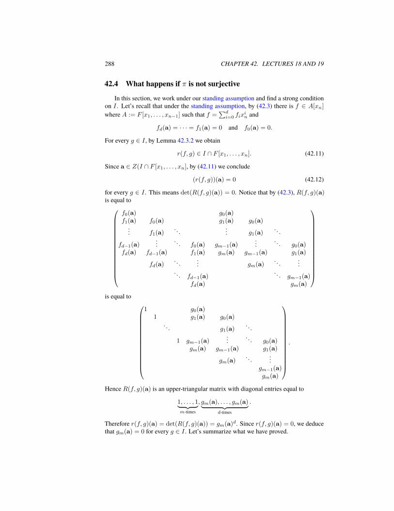
288 CHAPTER 42. LECTURES 18 AND 19
42.4 What happens if π is not surjective
In this section, we work under our standing assumption and find a strong conditionon I . Let’s recall that under the standing assumption, by (42.3) there is f ∈ A[xn]
where A := F [x1, . . . , xn−1] such that f =∑di=0 fix
in and
fd(a) = · · · = f1(a) = 0 and f0(a) = 0.
For every g ∈ I , by Lemma 42.3.2 we obtain
r(f, g) ∈ I ∩ F [x1, . . . , xn]. (42.11)
Since a ∈ Z(I ∩ F [x1, . . . , xn], by (42.11) we conclude
(r(f, g))(a) = 0 (42.12)
for every g ∈ I . This means det(R(f, g)(a)) = 0. Notice that by (42.3), R(f, g)(a)is equal to
f0(a) g0(a)f1(a) f0(a) g1(a) g0(a)
... f1(a). . .
... g1(a). . .
fd−1(a)...
. . . f0(a) gm−1(a)...
. . . g0(a)fd(a) fd−1(a) f1(a) gm(a) gm−1(a) g1(a)
fd(a). . .
... gm(a). . .
.... . . fd−1(a)
. . . gm−1(a)fd(a) gm(a)
is equal to
1 g0(a)1 g1(a) g0(a)
. . . g1(a). . .
1 gm−1(a)...
. . . g0(a)gm(a) gm−1(a) g1(a)
gm(a). . .
...gm−1(a)gm(a)
.
Hence R(f, g)(a) is an upper-triangular matrix with diagonal entries equal to
1, . . . , 1︸ ︷︷ ︸m-times
, gm(a), . . . , gm(a)︸ ︷︷ ︸d-times
.
Therefore r(f, g)(a) = det(R(f, g)(a)) = gm(a)d. Since r(f, g)(a) = 0, we deducethat gm(a) = 0 for every g ∈ I . Let’s summarize what we have proved.

42.5. FINDING A SUITABLE LINEAR CHANGE OF COORDINATES 289
Lemma 42.4.1. SupposeF is an algebraically closed field, I is an ideal ofF [x1, . . . , xn],a ∈ Z(I ∩ F [x1, . . . , xn−1], and π−1(a) = ∅ where
π : Z(I)→ Z(I ∩ F [x1, . . . , xn−1]), π(a1, . . . , an) := (a1, . . . , an−1).
Then for every g =∑mi=0 gix
in ∈ I with gi ∈ F [x1, . . . , xn−1] and gm 6= 0, we have
gm(a) = 0.
42.5 Finding a suitable linear change of coordinates
In this section, we show that after a linear change of coordinates, we can findg = gmx
mn + · · · g1xn + g0 in I such that gm is a non-zero constant. By this result and
Lemma 42.4.1, we conclude that π is surjective. This in turn shows that Z(I) is notempty.
Lemma 42.5.1. Suppose F is an infinite field, and h ∈ F [x1, . . . , xn] \ F .
1. For every ~α := (α1, . . . , αn−1) ∈ Fn−1, θ~α : F [x1, . . . , xn]→ F [x1, . . . , xn],
θ~α(f) := f(x1 + α1xn, . . . , xn−1 + αn−1xn, xn)
is an F -isomorphism.
2. There is ~α ∈ Fn−1 such that
θ~α(f) = cxmn + hm−1xm−1 + · · ·+ h0
for some hi’s in F [x1, . . . , xn−1] and c ∈ F×.
Proof. (1) Notice that for ~α, ~β ∈ Fn−1,
θ~α ◦ θ~β(f) =θ~β(x1 + α1xn, . . . , xn−1 + αn−1xn, xn)
=f(x1 + α1xn + β1xn, . . . , xn−1 + αn−1xn + βn−1xn, xn)
=θ~α+~β(f).
In particular, θ~α ◦ θ−~α = θ−~α ◦ θ~α = id, which implies that θ~α is bijective. It is easyto check that θ~α is an F -linear ring homomorphism.
(2) Since θ~α is an F -linear map and every polynomial is an F -linear combinationof monomials, we start with understanding θ~α(xi) where xi := xi11 · · ·xinn . We have
θ~α(xi) =
n−1∏j=1
(xj + αjxn)ij · xinn
=( n−1∏j=1
(αj)ij)xmn + rm−1x
m−1n + · · ·+ r0, (42.13)
wherem = i1+· · ·+in and ri’s are inF [x1, . . . , xn−1]. The summation i1+· · ·+in iscalled the total degree of the monomial xi and it is denoted by either degxi or ‖i‖1. By
290 CHAPTER 42. LECTURES 18 AND 19
(42.13), the coefficient of x‖i‖1n in θ~α(xi) is φ~α′(xi) where ~α′ := (α1, . . . , αn−1, 1);this means it is xi evaluated at ~α′. Another consequence of (42.13) is that the degreeof θ~α′(xi) as a polynomial in terms of the variable xn is at most ‖i‖1.
Suppose h =∑
i cixi. Then
θ~α(h) =∑i
ciθ~α′(xi)
=∑i
ci(φ~α′(xi)x‖i‖1n + pi(xn)), (42.14)
where pi(xn) ∈ (F [x1, . . . , xn−1])[xn] is a polynomial of degree at most ‖i‖1 − 1.The total degree of h is defined to be
max{‖i‖ | ci 6= 0},
and it is denoted by deg h. Suppose m := deg h, and let
h :=∑‖i‖1=m
cixi;
this means h is the sum of all the monomials of h that have the maximum possible totaldegree. Then by (42.14), we conclude that
θ~α(h) =∑‖i‖1=m
ciφ~α′(xi)xmn + p(xn)
=φ~α′(∑‖i‖1=m
cixi)xmn + p(xn)
=h(~α′)xmn + p(xn), (42.15)
where p(xn) ∈ (F [x1, . . . , xn−1])[xn] is a polynomial of degree at most m− 1. Nextwe will find ~α such that h(~α′) 6= 0. By this result and (42.15), we will finish the proofof Lemma.
Claim. If F is an infinite field and h′ ∈ F [x1, . . . , xk] \ {0}, then h′(~α) 6= 0 forsome ~α ∈ F k.
Proof of Claim. We proceed by induction on the number k of variables. By Corol-lary 7.1.5, a single variable polynomial of degree m in F [x] has at most m distinctzeros in F . Since F is an infinite field, h′(α) 6= 0 for some α ∈ F . Next we show theinduction step. Suppose
h′
= hmxmk + · · ·+ h0
for some hi’s in F [x1, . . . , xk−1] and hm 6= 0. By the induction hypothesis,
hm(α1, . . . , αk−1) 6= 0
for some αi’s in F . Hence
h′(α1, . . . , αk−1, xk) = hm(α1, . . . , αk−1)xmk + · · ·+ h0(α1, . . . , αk−1)

42.6. HILBERT’S NULLSTELLENSATZ 291
is a non-zero single variable polynomial. Therefore by the single variable case,
h′(α1, . . . , αk−1, αk) 6= 0
for some αk ∈ F . This completes proof of the Claim.
To finish proof of Lemma 42.5.1, we let
h′(x1, . . . , xn−1) := h(x1, . . . , xn−1, 1).
Notice that since all the monomials of h have the same total degree, h′ is a non-zeropolynomial. Hence by the above Claim, h′(~α) 6= 0 for some ~α ∈ Fn−1. Thereforeh(~α′) 6= 0. Thus by (42.15), we deduce that θ~α(h) has the desired form. This completesthe proof.
It is worth pointing out that θ~α(f) is evaluating f at1 −α1
. . ....
1 −αn−1
1
x1
...xn−1
xn
This is another hidden relation of our argument for higher degree polynomial equationsand the reduced row-column process.
42.6 Hilbert’s Nullstellensatz
In this section, we prove Hilbert’s Nullstellensatz which gives us the necessaryand sufficient condition for a system of polynomial equations to have a zero over analgebraically closed field.
Theorem 42.6.1 (Hilbert’s Nnullstellensatz, v.1). Suppose F is an algebraically closedfield, and I is an ideal of F [x1, . . . , xn]. Then Z(I) 6= ∅ if and only if 1 6∈ I .
Proof. (⇒) If 1 ∈ I , then Z(I) = ∅.(⇐) We proceed by induction on the number n of variables. For the base of
induction, we notice that F [x1] is a PID. Hence I = 〈p(x1)〉 for some polynomial p.Since 1 6∈ I , p is not a nonn-zero constant polynomial. As F is algebraically closed, phas a zero in F . Therefore Z(I) 6= ∅. Next we prove the induction step. If I = 0, thenZ(I) = Fn, and there is nothing to prove. So we can and will assume that there is anon-constant polynomial h in I . By Lemma 42.5.1, there is ~α ∈ Fn−1 such that
θ~α(h) = cxmn + hm−1xm−1n + · · ·+ h0 (42.16)
for some hi’s in F [x1, . . . , xn−1] and c ∈ F×. Since θ~α is an isomorphism (seeLemma 42.5.1), θ~α(I) is an ideal of F [x1, . . . , xn]. By (42.16) and Lemma 42.5.1,π : Z(θ~α(I))→ Z(θ~α(I) ∩ F [x1, . . . , xn−1]),
π(a1, . . . , an) = (a1, . . . , an−1).
292 CHAPTER 42. LECTURES 18 AND 19
is surjective. Since 1 6∈ I , 1 6∈ θ~α(I). Therefore 1 6∈ θ~α(I ∩ F [x1, . . . , xn−1]). Henceby the induction hypothesis, Z(θ~α(I) ∩ F [x1, . . . , xn−1]) 6= ∅. Since π is surjective,Z(θ~α(I)) 6= ∅. Notice that
(a1, . . . , an) ∈ Z(θ~α(I))⇔∀f ∈ I, θ~α(f)(a1, . . . , an) = 0
⇔∀f ∈ I, f(a1 + α1an, . . . , an−1 + αn−1an, an) = 0
⇔(a1 + α1an, . . . , an−1 + αn−1an, an) ∈ Z(I).
Therefore Z(I) 6= ∅. This completes the proof.
Hilbert’s Nullstellensatz has many implications. For instance we can classify allthe maximal ideals of F [x1, . . . , xn] when F is algebraically closed.
Theorem 42.6.2 (Hilbert’s Nullstellensatz, v.2). Suppose F is an algebraically closedfield. Then the following is a bijection:
Fn → Max(F [x1, . . . , xn]), a 7→ I({a}),
where Max(·) is the set of all the maximal ideals. Moreover
I(a1, . . . , an) = 〈x1 − a1, . . . , xn − an〉.
Proof. For a ∈ Fn, let φa : F [x1, . . . , xn]→ F be the map of evaluation at a. Thenby the first isomorphism theorem,
F [x1, . . . , xn]/ kerφa ' F.
Hence kerφa ∈ Max(F [x1, . . . , xn]). Notice that kerφa = I({a}). Therefore thegiven map is well-defined.
Next we show injectivity. Notice that xi − ai’s are in I({a}) if a = (a1, . . . , an).Hence Z(I({a})) = {a}. Therefore I({a}) = I({a′}) implies that a = a′, and wededuce the injectivity.
Finally we show the surjectivity. Suppose M ∈ Max(F [x1, . . . , xn]). Then byHilbert’s Nullstellensatz, version 1, there is a ∈ Z(M). Hence M ⊆ I({a}). BecauseM is a maximal ideal, M ⊆ I({a}), and I({a}) is a proper ideal, we conclude thatM = I({a}). We obtain the surjectivity.
Since xi − ai’s are in I({a}) where a := (a1, . . . , an), we have that
〈x1 − a1, . . . , xn − an〉 ⊆ I({a}). (42.17)
Notice that Ld(xi − ai) = xi. Hence every non-constant monomial is in the idealgenerated by Ld(xi − ai)’s. Since I({a}) is a proper ideal, for every f ∈ I \ {0},Ld(f) is a non-constant monomial. Therefore
Ld(f) ∈ 〈Ld(x1 − a1), . . . ,Ld(xn − an)〉 (42.18)
for every f ∈ I({a}). By (42.17), (42.18), and Lemma 41.1.3, we deduce that
〈x1 − a1, . . . , xn − an〉 = I({a}).
This completes the proof.
42.6. HILBERT’S NULLSTELLENSATZ 293
Using the second version of Hilbert’s Nullstellensatz, we can understand points ofZ(I) in terms of maximal ideals.
Theorem 42.6.3 (Hilbert’s Nullstellensatz, v.3). Suppose F is an algebraically closedfield and I is an ideal ofF [x] := F [x1, . . . , xn]. Then the following maps are bijections:
Z(I)→ {M ∈ Max(F [x]) | I ⊆M}, a 7→ I({a}), (42.19)
{M ∈ Max(F [x]) | I ⊆M} → Max(F [x]
I
), M 7→ M
I, (42.20)
andZ(I)→ Max
(F [x]
I
), a 7→ I({a})
I. (42.21)
Proof. For every a ∈ Z(I), we have that I ⊆ I(a). By the second version of Hilbert’sNullstellensatz, I({a}) is in Max(F [x]). Therefore the map given in (42.19) is well-defined. By the second version of Hilbert’s Nullstellensatz, a 7→ I({a}) is injective.Next we show surjectivity of the map given in (42.19). Suppose M ∈ Max(F [x]) andI ⊆ M . Then by the second version of Hilbert’s Nullstellensatz, M = I({a}) forsome a ∈ Fn. So I ⊆ I({a}), which means a ∈ Z(I). This shows that the map givenin (42.19) is surjective.
By Lemma 9.3.4, we know that the following is a bijection
{J E F [x] | I ⊆ J} →{J E
F [x]
I
}, J 7→ J
I. (42.22)
Since this bijection preserves inclusion, we deduce that it sends maximal ideals tomaximal ideals. Hence the function given in (42.20) is a bijection.
The map given in (42.21) is the composite of the bijections given in (42.19) and(42.20). Hence it is a bijection. This completes the proof.
Another version of Hilbert’s Nullstellensatz gives us a complete understanding ofI(Z(I)). This means that it answers the following question:
What are the polynomials that vanish on the common zeros of elements of I?Notice that if fn ∈ I for some positive integer n, then fn|Z(I) = 0. Hence
f |Z(I) = 0, which means that
{f ∈ F [x] | fn ∈ Ifor some positive integer n} ⊆ I(Z(I)). (42.23)
The left hand side of the inclusion given in (42.23) is called the radical of I and itis denoted by
√I . Our final version of Hilbert’s Nullstellensatz states the equality in
(42.23) holds.
Theorem 42.6.4 (Hilbert’s Nullstellensatz, v.4). Suppose F is an algebraically closedfield and I is an ideal of F [x1, . . . , xn]. Then I(Z(I)) =
√I .
Proof. By (42.23), we have that√I ⊆ I(Z(I)). Now assume that f 6∈
√I . We want
to show that f 6∈ I(Z(I)). This means we would like to show that there is a ∈ Fn

294 CHAPTER 42. LECTURES 18 AND 19
such that for every g ∈ I , g(a) = 0 and f(a) 6= 0. Since an element of F is non-zeroif and only if it is a unit, we are looking for a ∈ Fn and b ∈ F such that
g(a) = 0 for every g ∈ I and f(a)b = 1. (42.24)
Existence of (a, b) ∈ Fn × F so that (42.24) holds is equivalent saying that thefollowing system of polynomial equations
g(x) = 0 for every g ∈ I and f(x)y − 1 = 0 (42.25)
have a common zero in Fn+1. By the first version of. Hilbert’s Nullstellensatz, thesystem of equations given in (42.25) has a common zero in Fn+1 if and only if theideal J generated by I and f(x)y − 1 in (F [x])[y] is a proper ideal. Suppose to thecontrary that 1 ∈ J . This implies that
1 = f1r1(y) + · · ·+ fkrk(y) + (fy − 1)s(y) (42.26)
for some fi’s inF [x] and r1, . . . , rk, s ∈ (F [x])[y]. Consider 1f in the fieldF (x1, . . . , xn)
of fractions of F [x1, . . . , xn], and evaluate ri’s and s at 1f . This means we consider
the map of evaluation at 1f
φ 1f
: (F [x])[y]→ F (x), φ 1f
(r) := r( 1
f
),
and apply it to the both sides of (42.26). This way, we obtain
1 = f1r1
( 1
f
)+ · · ·+ fkrk
( 1
f
). (42.27)
Notice that ri( 1f ) = pi
fdifor some pi ∈ F [x] and di ∈ Z+. LetN := max(d1, . . . , dk).
Then multiplying both sides of (42.27) by fN , we obtain that
fN = f1q1 + · · ·+ fkqk
for some qi’s in F [x]. Therefore fN is in the ideal generated by fi’s. Hence fN ∈ Ias fi’s are in I . This implies that f ∈
√I , which is a contradiction. This completes the
proof.
Notice that if P is a prime ideal, then√P = P . This is the case as for a prime
ideal P , fn ∈ P for some positive integer n implies that f ∈ P . Hence by the fourthversion of Hilbert’s Nullstellensatz, we have
I(Z(P )) = P
for every prime ideal P of F [x] when F is an algebraically closed field F .Here is an interesting consequence of Hilbert’s Nullstellensatz in ring theory.
Proposition 42.6.5. Suppose F is an algebraically closed field. Then for every primeideal P of F [x1, . . . , xn], we have
P =⋂
M∈Max(F [x]),P⊆M
M.
42.7. FINAL REMARKS 295
Proof. By the fourth version of Hilbert’s Nullstellensatz, we have P = I(Z(P )).Hence
P = I(Z(P )) =⋂
a∈Z(P )
I({a}) =⋂
M∈Max(F [x]),P⊆M
M
where the last equality holds because of the third version of Hilbert’s Nullstellensatz.This completes the proof.
42.7 Final remarks
Let’s finish by mentioning that not surprisingly zeros of multivariable polynomialsare much more complicated than their single variable counterpart. In the single variablecase, Z(I) is either a finite set or F . Many of the interesting surfaces or manifolds thatwe know can be viewed as the set of real or complex zeros certain system of polynomialequations. Here are some examples:
1. Sphere: x2 + y2 + z2 = 1.
2. Special linear group: SLn(C) := {A ∈ Mn(C) | detA = 1}.
3. A curve related to Fermat’s last conjecture: Xn + Y n = 1.
4. Equation related to Markoff triples: x2 + y2 + z2 = 3xyz.
5. Elliptic curves: y2 = x3 + ax+ b.
Thinking about these equations from geometric point of view gives us the neededlanguage to ask many interesting questions, helps us use results and tools from geometryand topology, and brings us many unexpected connections.