Embed Size (px)
Citation preview
ALF User’s Manual
Michael Hanus
Informatik II
RWTH Aachen
D-52056 Aachen, Germany
Andreas Schwab
Informatik V
Universitat Dortmund
D-44221 Dortmund, Germany
August 18, 1995
1
Contents
1 Introduction 4
2 An introductory example 5
3 Syntax of ALF 7
3.1 Context free grammar . . . . . . . . . . . . . . . . . . . . . . . . . . . . . . . . . . . 7
3.2 Syntactic restrictions . . . . . . . . . . . . . . . . . . . . . . . . . . . . . . . . . . . . 9
3.3 Lists and operators . . . . . . . . . . . . . . . . . . . . . . . . . . . . . . . . . . . . . 10
3.4 The type system . . . . . . . . . . . . . . . . . . . . . . . . . . . . . . . . . . . . . . 11
3.5 The module concept . . . . . . . . . . . . . . . . . . . . . . . . . . . . . . . . . . . . 12
3.6 Semantic restrictions . . . . . . . . . . . . . . . . . . . . . . . . . . . . . . . . . . . . 13
4 Semantics 14
5 Examples 18
5.1 Natural numbers . . . . . . . . . . . . . . . . . . . . . . . . . . . . . . . . . . . . . . 18
5.2 Polymorphic lists . . . . . . . . . . . . . . . . . . . . . . . . . . . . . . . . . . . . . . 18
5.3 Stacks . . . . . . . . . . . . . . . . . . . . . . . . . . . . . . . . . . . . . . . . . . . . 19
5.4 A generic sort module . . . . . . . . . . . . . . . . . . . . . . . . . . . . . . . . . . . 19
6 Predefined functions and predicates 20
6.1 The module string . . . . . . . . . . . . . . . . . . . . . . . . . . . . . . . . . . . . 20
6.2 The module term . . . . . . . . . . . . . . . . . . . . . . . . . . . . . . . . . . . . . . 21
6.3 The module operator . . . . . . . . . . . . . . . . . . . . . . . . . . . . . . . . . . . 22
6.4 The module streamio . . . . . . . . . . . . . . . . . . . . . . . . . . . . . . . . . . . 23
6.5 The module system . . . . . . . . . . . . . . . . . . . . . . . . . . . . . . . . . . . . 24
7 How to use the current system 24
7.1 Files . . . . . . . . . . . . . . . . . . . . . . . . . . . . . . . . . . . . . . . . . . . . . 25
7.2 Compiling ALF programs . . . . . . . . . . . . . . . . . . . . . . . . . . . . . . . . . 25
7.3 Executing and debugging ALF programs . . . . . . . . . . . . . . . . . . . . . . . . . 26
8 Restrictions and bugs 29
2
List of Tables
1 Reserved words and symbols . . . . . . . . . . . . . . . . . . . . . . . . . . . . . . . 10
2 List notations in ALF . . . . . . . . . . . . . . . . . . . . . . . . . . . . . . . . . . . 10
3 Predefined operators in ALF clauses . . . . . . . . . . . . . . . . . . . . . . . . . . . 11
List of Figures
1 Operational semantics of ALF . . . . . . . . . . . . . . . . . . . . . . . . . . . . . . . 16
2 Module string . . . . . . . . . . . . . . . . . . . . . . . . . . . . . . . . . . . . . . . 20
3 Module term . . . . . . . . . . . . . . . . . . . . . . . . . . . . . . . . . . . . . . . . 21
4 Module operator . . . . . . . . . . . . . . . . . . . . . . . . . . . . . . . . . . . . . . 22
5 Module streamio . . . . . . . . . . . . . . . . . . . . . . . . . . . . . . . . . . . . . . 23
6 Module system . . . . . . . . . . . . . . . . . . . . . . . . . . . . . . . . . . . . . . . 24
3
1 Introduction
ALF (Algebraic Logic Functional programming language) is a language which combines functional
and logic programming techniques. The foundation of ALF is Horn clause logic with equality which
consists of predicates and Horn clauses for logic programming, and functions and equations for
functional programming. Since ALF is a genuine integration of both programming paradigms, any
functional expression can be used in a goal literal and arbitrary predicates can occur in conditions
of equations. The operational semantics of ALF is based on the resolution rule to solve literals and
narrowing to evaluate functional expressions. In order to reduce the number of possible narrowing
steps, a leftmost-innermost basic narrowing strategy is used which can be efficiently implemented.
Furthermore, terms are simplified by rewriting before a narrowing step is applied and also equations
are rejected if the two sides have different constructors at the top. Rewriting and rejection can
result in a large reduction of the search tree. Therefore this operational semantics is more efficient
than Prolog’s resolution strategy.
The ALF system is an efficient implementation of the combination of resolution, nar-
rowing, rewriting and rejection. Similarly to Prolog, ALF uses a backtracking strategy corre-
sponding to a depth-first search in the derivation tree. ALF programs are compiled into instructions
of an abstract machine. The abstract machine is based on the Warren Abstract Machine (WAM)
with several extensions to implement narrowing and rewriting. In the current implementation
programs of this abstract machine are executed by an emulator written in C.
ALF has also a type and module concept which allows the definition of generic modules. A
preprocessor checks the type consistence of the program and combines all needed modules into one
flat-ALF program which is compiled into a compact bytecode representing an abstract machine
program. The current implementation has the following properties:
• The machine code for pure logic programs without defined functions is identical to the code
of the original WAM [War83], i.e., for logic programs there is no overhead because of the
functional part of the language.
• Functional programs where only ground terms have to be evaluated are executed by determin-
istic rewriting without any dynamic search for subterms positions where the next rewriting
step can be applied. The compiler computes these positions and generates particular machine
instructions. Therefore such programs are also efficiently executed.
• In mixed functional and logic programs argument terms are simplified by rewriting before
narrowing is applied and therefore function calls with ground arguments are automatically
evaluated by rewriting and not by narrowing. This is more efficient because rewriting is
a deterministic process. Hence in most practical cases the combined rewriting/narrowing
implementation is more efficient than an implementation of narrowing by flattening terms
and applying SLD-resolution [Han91, Han92].
This manual describes the syntax and semantics of ALF. Moreover, it contains a detailed description
of the current implementation of the ALF system from a user’s point of view. Details about the
implementation technique (i.e., the abstract machine and compilation of ALF programs into this
machine) can be found in [Han90, Han91]. The current system is available from the first author.
4
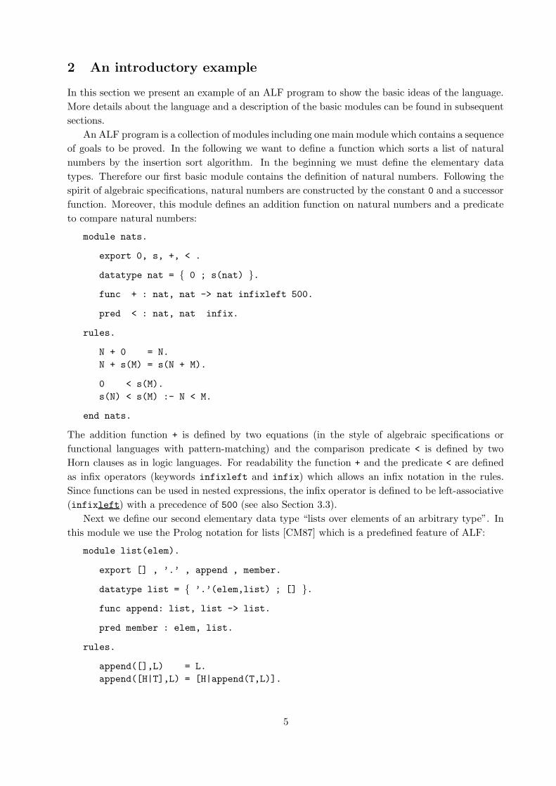
2 An introductory example
In this section we present an example of an ALF program to show the basic ideas of the language.
More details about the language and a description of the basic modules can be found in subsequent
sections.
An ALF program is a collection of modules including one main module which contains a sequence
of goals to be proved. In the following we want to define a function which sorts a list of natural
numbers by the insertion sort algorithm. In the beginning we must define the elementary data
types. Therefore our first basic module contains the definition of natural numbers. Following the
spirit of algebraic specifications, natural numbers are constructed by the constant 0 and a successor
function. Moreover, this module defines an addition function on natural numbers and a predicate
to compare natural numbers:
module nats.
export 0, s, +, < .
datatype nat = { 0 ; s(nat) }.
func + : nat, nat -> nat infixleft 500.
pred < : nat, nat infix.
rules.
N + 0 = N.
N + s(M) = s(N + M).
0 < s(M).
s(N) < s(M) :- N < M.
end nats.
The addition function + is defined by two equations (in the style of algebraic specifications or
functional languages with pattern-matching) and the comparison predicate < is defined by two
Horn clauses as in logic languages. For readability the function + and the predicate < are defined
as infix operators (keywords infixleft and infix) which allows an infix notation in the rules.
Since functions can be used in nested expressions, the infix operator is defined to be left-associative
(infixleft) with a precedence of 500 (see also Section 3.3).
Next we define our second elementary data type “lists over elements of an arbitrary type”. In
this module we use the Prolog notation for lists [CM87] which is a predefined feature of ALF:
module list(elem).
export [] , ’.’ , append , member.
datatype list = { ’.’(elem,list) ; [] }.
func append: list, list -> list.
pred member : elem, list.
rules.
append([],L) = L.
append([H|T],L) = [H|append(T,L)].
5
member(E,[E|_]).
member(E,[_|L]) :- member(E,L).
end list.
The type of the list elements is a parameter to this module, i.e., list is a generic module. It exports
the list contructors [] and ’.’, a function to concatenate two lists and a member predicate on
lists.
Now it would be possible to define our sort function on lists but for convenience we define a
further module which extends the module nats by defining some additional predicates to compare
natural numbers:
module natord.
export 0 , s , + , < , > , =/= , =< , >= .
use nats.
pred > : nat, nat infix;
=/= : nat, nat infix;
=< : nat, nat infix;
>= : nat, nat infix.
rules.
N > M :- M < N.
N =/= M :- N < M.
N =/= M :- N > M.
N =< N.
N =< M :- N < M.
N >= N.
N >= M :- N > M.
end natord.
This module imports the module nats by the declaration “use nats” and exports all objects
defined in module nats and the additional predicates defined in this module. Now we declare our
main module containing the definition of the sort function on lists of naturals:
module isort.
export isort.
use natord;
list(nat).
func isort : list -> list;
insert: nat, list -> list.
rules.
isort([]) = [].
isort([E|L]) = insert(E,isort(L)).
insert(E,[]) = [E].
insert(E,[F|L]) = [E,F|L] :- E =< F.
insert(E,[F|L]) = [F|insert(E,L)] :- E > F.
6
end isort.
?- isort([3,1,5,4,1,3,2]) = L.
This module imports the modules natord and list where the generic list module is used with
the actual sort parameter nat (imported from natord). The sort function isort is specified by
two equations where the second equation uses the function insert to insert an element at the
appropriate position in an ordered list. The definition of insert uses conditional equations which
is a standard feature of ALF since ALF is a genuine integration of functional and logic languages.
At the end of this main module the goal to be proved by the ALF system is appended. Note that
natural numbers need not be written down as s-terms since ALF translates natural numbers like
3 into equivalent s-terms like s(s(s(0))).
If the main module and all imported modules are translated by the ALF system and the compiled
program is executed, we get the answer
isort([3,1,5,4,1,3,2]) = [1,1,2,3,3,4,5]
which is a logical consequence of our program (see Section 4 for the operational semantics of ALF).
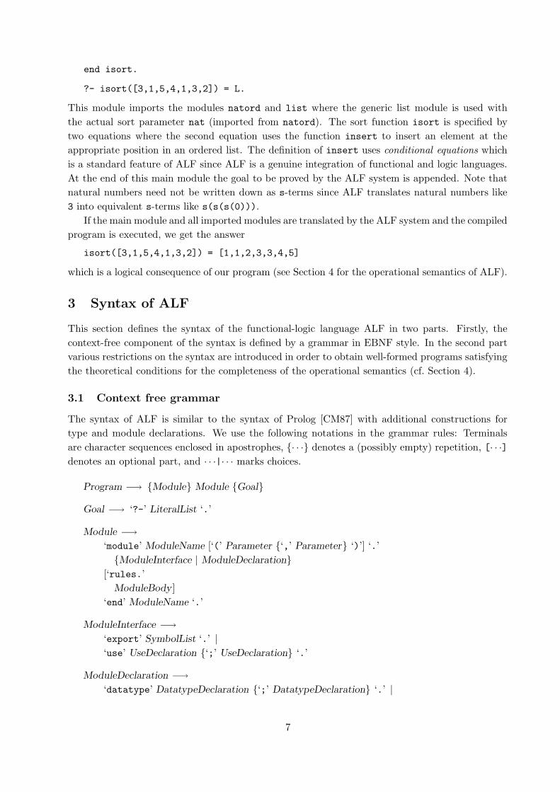
3 Syntax of ALF
This section defines the syntax of the functional-logic language ALF in two parts. Firstly, the
context-free component of the syntax is defined by a grammar in EBNF style. In the second part
various restrictions on the syntax are introduced in order to obtain well-formed programs satisfying
the theoretical conditions for the completeness of the operational semantics (cf. Section 4).
3.1 Context free grammar
The syntax of ALF is similar to the syntax of Prolog [CM87] with additional constructions for
type and module declarations. We use the following notations in the grammar rules: Terminals
are character sequences enclosed in apostrophes, {· · ·} denotes a (possibly empty) repetition, [· · ·]
denotes an optional part, and · · ·|· · · marks choices.
Program −→ {Module} Module {Goal}
Goal −→ ‘?-’ LiteralList ‘.’
Module −→
‘module’ ModuleName [‘(’ Parameter {‘,’ Parameter} ‘)’] ‘.’
{ModuleInterface | ModuleDeclaration}
[‘rules.’
ModuleBody ]
‘end’ ModuleName ‘.’
ModuleInterface −→
‘export’ SymbolList ‘.’ |
‘use’ UseDeclaration {‘;’ UseDeclaration} ‘.’
ModuleDeclaration −→
‘datatype’ DatatypeDeclaration {‘;’ DatatypeDeclaration} ‘.’ |
7
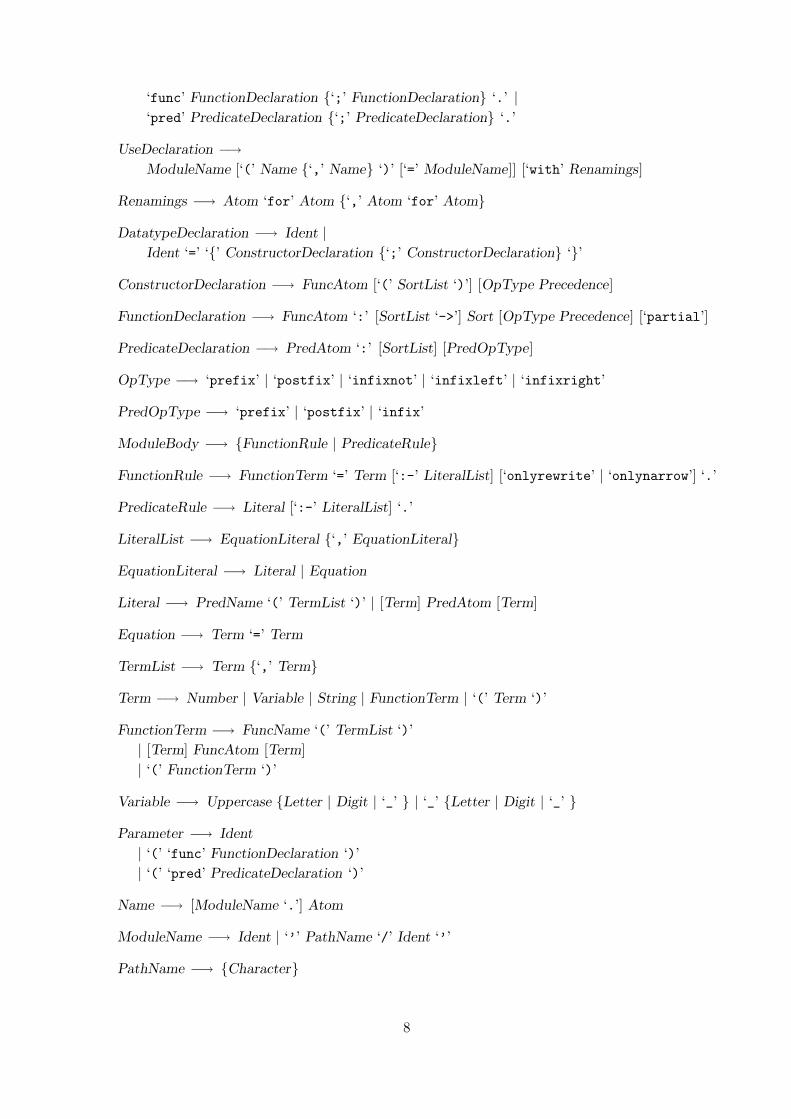
‘func’ FunctionDeclaration {‘;’ FunctionDeclaration} ‘.’ |
‘pred’ PredicateDeclaration {‘;’ PredicateDeclaration} ‘.’
UseDeclaration −→
ModuleName [‘(’ Name {‘,’ Name} ‘)’ [‘=’ ModuleName]] [‘with’ Renamings]
Renamings −→ Atom ‘for’ Atom {‘,’ Atom ‘for’ Atom}
DatatypeDeclaration −→ Ident |
Ident ‘=’ ‘{’ ConstructorDeclaration {‘;’ ConstructorDeclaration} ‘}’
ConstructorDeclaration −→ FuncAtom [‘(’ SortList ‘)’] [OpType Precedence]
FunctionDeclaration −→ FuncAtom ‘:’ [SortList ‘->’] Sort [OpType Precedence] [‘partial’]
PredicateDeclaration −→ PredAtom ‘:’ [SortList] [PredOpType]
OpType −→ ‘prefix’ | ‘postfix’ | ‘infixnot’ | ‘infixleft’ | ‘infixright’
PredOpType −→ ‘prefix’ | ‘postfix’ | ‘infix’
ModuleBody −→ {FunctionRule | PredicateRule}
FunctionRule −→ FunctionTerm ‘=’ Term [‘:-’ LiteralList] [‘onlyrewrite’ | ‘onlynarrow’] ‘.’
PredicateRule −→ Literal [‘:-’ LiteralList] ‘.’
LiteralList −→ EquationLiteral {‘,’ EquationLiteral}
EquationLiteral −→ Literal | Equation
Literal −→ PredName ‘(’ TermList ‘)’ | [Term] PredAtom [Term]
Equation −→ Term ‘=’ Term
TermList −→ Term {‘,’ Term}
Term −→ Number | Variable | String | FunctionTerm | ‘(’ Term ‘)’
FunctionTerm −→ FuncName ‘(’ TermList ‘)’
| [Term] FuncAtom [Term]
| ‘(’ FunctionTerm ‘)’
Variable −→ Uppercase {Letter | Digit | ‘_’ } | ‘_’ {Letter | Digit | ‘_’ }
Parameter −→ Ident
| ‘(’ ‘func’ FunctionDeclaration ‘)’
| ‘(’ ‘pred’ PredicateDeclaration ‘)’
Name −→ [ModuleName ‘.’] Atom
ModuleName −→ Ident | ‘’’ PathName ‘/’ Ident ‘’’
PathName −→ {Character}
8
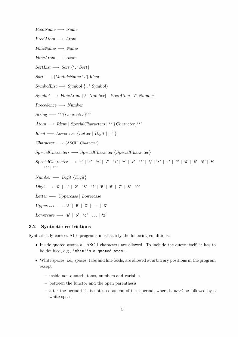
PredName −→ Name
PredAtom −→ Atom
FuncName −→ Name
FuncAtom −→ Atom
SortList −→ Sort {‘,’ Sort}
Sort −→ [ModuleName ‘.’] Ident
SymbolList −→ Symbol {‘,’ Symbol}
Symbol −→ FuncAtom [‘/’ Number] | PredAtom [‘/’ Number]
Precedence −→ Number
String −→ ‘"’{Character}‘"’
Atom −→ Ident | SpecialCharacters | ‘’’{Character}‘’’
Ident −→ Lowercase {Letter | Digit | ‘_’ }
Character −→ 〈ASCII–Character〉
SpecialCharacters −→ SpecialCharacter {SpecialCharacter}
SpecialCharacter −→ ‘+’ | ‘-’ | ‘*’ | ‘/’ | ‘<’ | ‘=’ | ‘>’ | ‘‘’ | ‘\’ | ‘:’ | ‘.’ | ‘?’ | ‘@’ | ‘#’ | ‘$’ | ‘&’
| ‘^’ | ‘~’
Number −→ Digit {Digit}
Digit −→ ‘0’ | ‘1’ | ‘2’ | ‘3’ | ‘4’ | ‘5’ | ‘6’ | ‘7’ | ‘8’ | ‘9’
Letter −→ Uppercase | Lowercase
Uppercase −→ ‘A’ | ‘B’ | ‘C’ | . . . | ‘Z’
Lowercase −→ ‘a’ | ‘b’ | ‘c’ | . . . | ‘z’
3.2 Syntactic restrictions
Syntactically correct ALF programs must satisfy the following conditions:
• Inside quoted atoms all ASCII characters are allowed. To include the quote itself, it has to
be doubled, e.g., ’that’’s a quoted atom’.
• White spaces, i.e., spaces, tabs and line feeds, are allowed at arbitrary positions in the program
except
– inside non-quoted atoms, numbers and variables
– between the functor and the open parenthesis
– after the period if it is not used as end-of-term period, where it must be followed by a
white space
9
• Comments are marked with the character %. All text between % and the end of the line is
ignored. Another way to mark a comment is to enclose it with /* and */. Inside atoms these
characters are not interpreted as comment characters.
• The following restrictions must hold for any ALF program and are checked by the ALF
system:
– The names after module at the beginning of a module and after end at the end must be
the same.
– In an application of a function, a predicate, or a constructor to terms the arity and the
types of the terms must coincide with the declaration (cf. Section 3.4).
– The identifiers in an export list must be distinct from each other and declared or im-
ported in this module.
– Every sort, constructor, function and predicate must be declared before its use.
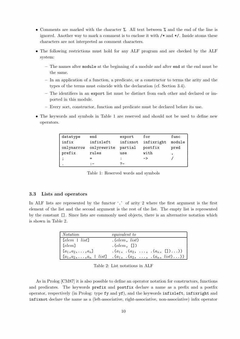
• The keywords and symbols in Table 1 are reserved and should not be used to define new
operators.
datatype end export for func
infix infixleft infixnot infixright module
onlynarrow onlyrewrite partial postfix pred
prefix rules use with ,
; = : -> /
. :- ?-
Table 1: Reserved words and symbols
3.3 Lists and operators
In ALF lists are represented by the functor ‘.’ of arity 2 where the first argument is the first
element of the list and the second argument is the rest of the list. The empty list is represented
by the constant []. Since lists are commonly used objects, there is an alternative notation which
is shown in Table 2.
Notation equivalent to
[elem | list] .(elem, list)[elem] .(elem, [])
[a1,a2,...,an] .(a1, .(a2, ..., .(an, [])...))
[a1,a2,...,an | list] .(a1, .(a2, ..., .(an, list)...))
Table 2: List notations in ALF
As in Prolog [CM87] it is also possible to define an operator notation for constructors, functions
and predicates. The keywords prefix and postfix declare a name as a prefix and a postfix
operator, respectively (in Prolog: type fy and yf), and the keywords infixleft, infixright and
infixnot declare the name as a (left-associative, right-associative, non-associative) infix operator
10
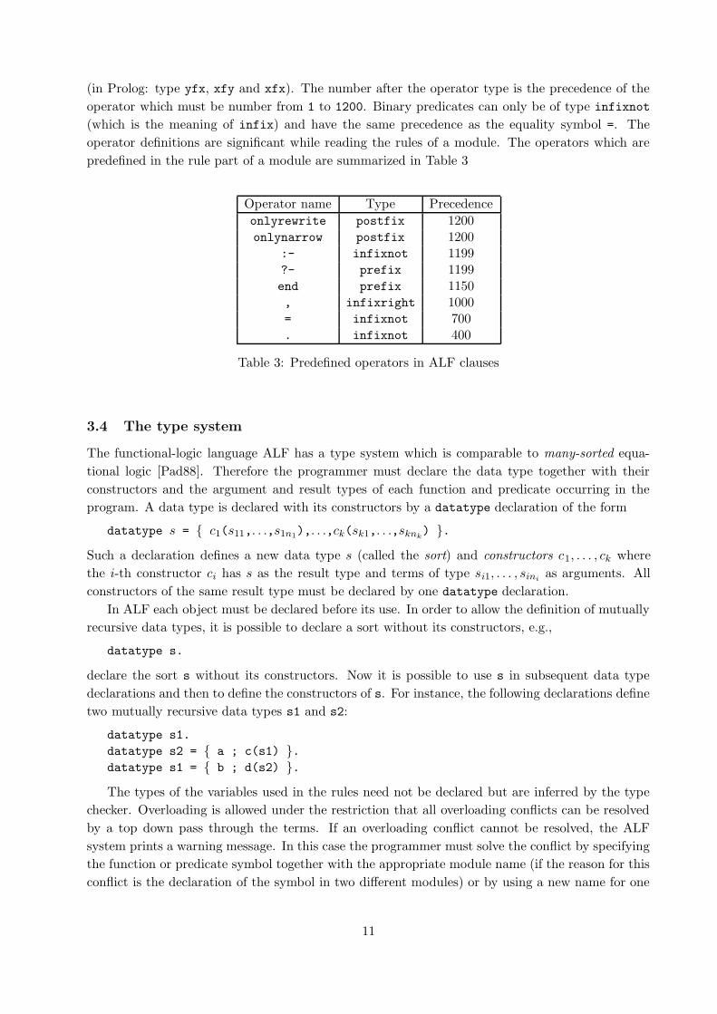
(in Prolog: type yfx, xfy and xfx). The number after the operator type is the precedence of the
operator which must be number from 1 to 1200. Binary predicates can only be of type infixnot
(which is the meaning of infix) and have the same precedence as the equality symbol =. The
operator definitions are significant while reading the rules of a module. The operators which are
predefined in the rule part of a module are summarized in Table 3
Operator name Type Precedence
onlyrewrite postfix 1200onlynarrow postfix 1200
:- infixnot 1199?- prefix 1199end prefix 1150, infixright 1000= infixnot 700. infixnot 400
Table 3: Predefined operators in ALF clauses
3.4 The type system
The functional-logic language ALF has a type system which is comparable to many-sorted equa-
tional logic [Pad88]. Therefore the programmer must declare the data type together with their
constructors and the argument and result types of each function and predicate occurring in the
program. A data type is declared with its constructors by a datatype declaration of the form
datatype s = { c1(s11,. . .,s1n1),. . .,ck(sk1,. . .,sknk
) }.
Such a declaration defines a new data type s (called the sort) and constructors c1, . . . , ck where
the i-th constructor ci has s as the result type and terms of type si1, . . . , sinias arguments. All
constructors of the same result type must be declared by one datatype declaration.
In ALF each object must be declared before its use. In order to allow the definition of mutually
recursive data types, it is possible to declare a sort without its constructors, e.g.,
datatype s.
declare the sort s without its constructors. Now it is possible to use s in subsequent data type
declarations and then to define the constructors of s. For instance, the following declarations define
two mutually recursive data types s1 and s2:
datatype s1.
datatype s2 = { a ; c(s1) }.datatype s1 = { b ; d(s2) }.
The types of the variables used in the rules need not be declared but are inferred by the type
checker. Overloading is allowed under the restriction that all overloading conflicts can be resolved
by a top down pass through the terms. If an overloading conflict cannot be resolved, the ALF
system prints a warning message. In this case the programmer must solve the conflict by specifying
the function or predicate symbol together with the appropriate module name (if the reason for this
conflict is the declaration of the symbol in two different modules) or by using a new name for one
11
of the symbols. Qualification is done by prefixing the function or predicate name with the module
name and a period: For instance, if the function f is defined in the modules m1 and m2 which
are imported into the main module, we can refer to the function f of module m2 by the notation
“m2.f”.
The language ALF offers also a kind of parametric polymorphism by allowing parameterized
modules. For instance, a module containing a definition of lists may be parameterized by the sort
of the elements (see Section 5.2). It is also allowed to have functions or predicates as module
parameters. E.g., a generic module for sorting lists of element have two parameters: the sort of
the elements and a binary predicate to compare two elements of this sort (see also Section 5.4).
But note that this concept of generic modules has nothing to do with parametric polymorphism:
it is a purely syntactic feature, i.e., if a parameterized module is used in another module, the text
of the parameterized module is copied with the actual parameters (however, ALF performs some
optimizations that avoids text copying if it is unnecessary).
3.5 The module concept
In order to implement large applications, ALF has a module concept to structure large programs. A
module is a collection of data type, function and predicate definitions together with a list of clauses
specifying the semantics of functions and predicates. If the module does not contain an export
declaration, all objects defined in this module are exported, otherwise only those constructors,
functions and predicates are exported which are listed in an export declaration. Sorts are implicitly
exported if an argument or result type of an exported object contains these sorts.
A module can be imported into another module by a use declaration. In this case all exported
objects of the imported module are visible inside the module. Note that if the module should
export some of the imported objects, it is necessary to list these imported objects in the export
declaration of the module, otherwise they are not visible outside this module. Example:
module m1.
export f.
datatype s = { · · · }.func f: s -> s;
g: s -> s.
rules.
% equations for f and g
end m1.
module m2.
export f, p.
use m1.
pred p: s, s.
rules.
% clauses for p
end m2.
Module m1 exports the function f and sort s, i.e., function g is invisible outside m1. Module m2
exports the imported function f, the imported sort s and the predicate p.
In order to have the complete specification of a function or predicate available in one module,
all defining clauses of a function or predicate must be stored in one module. Hence it is not allowed
to distribute the defining clauses of one function or predicate over several modules. Therefore the
12
ALF system outputs an error message if a module contains a clause where the function or predicate
in the left-hand side is a parameter (see below) or imported from other modules. For instance, it
is not allowed to write a clause “f(· · ·) = · · ·” inside module m2 in the example above.
If a module m imports two other modules ma and mb, it is possible that name conflicts occur
because ma and mb exports objects with identical names. In order to avoid such name conflicts,
ALF allows a renaming of objects when modules are imported. For instance, if both ma and mb
exports a function f, then we can rename these functions in the import declaration:
module m.
· · ·use ma with fma for f.
use mb with fmb for f.
· · ·
Now the function f of module ma is identified by the name fma in the body of module m. Another
solution to avoid name conflicts is to qualify names by the dot notation (cf. Section 3.4): If the
function f is not renamed in the use declaration, then we can refer by the notation “ma.f” to the
function f of module ma.
ALF modules can be parameterized by sorts, functions and predicates (see Section 3.4). Ex-
amples for such generic modules can be found in Sections 5.2, 5.3 and 5.4. If a generic module is
imported and instantiated with actual parameters and we want to refer to this instantiated module
(e.g., to avoid name conflicts using the dot notation), it is necessary to have a unique identifier for
this module. Therefore it is allowed to specify a new name for this instantiated module inside the
use declaration. For instance, if we import the generic list module (Section 5.2) with the actual
sort parameter nat, we can write
use list(nat) = natList.
and refer to the function append for lists of naturals by the notation “natList.append”. An
alternative solution is to rename the function append in the use declaration:
use list(nat) with natListAppend for append.
(it is also allowed to combine the renaming of a generic module with the renaming of some objects
of this module). Note that this renaming is only necessary if the type checker of ALF cannot resolve
name conflicts in subsequent clauses.
An important requirement to ALF modules is the persistency condition: all objects which are
imported in a module (where parameters are also considered as imported objects) are not modified
inside this module. In order to ensure this, it is not allowed to redefine imported sorts or to specify
equations or clauses for imported functions or predicates inside the module. These conditions are
checked by the ALF system.
Usually all modules are stored in one directory in the file system, but it is also possible to
distribute the modules in several directories. For details see remarks at beginning of Section 7.2.
3.6 Semantic restrictions
The following restrictions are necessary in order to ensure the completeness of the operational
semantics (cf. Section 4) (however, the implemented operational semantics is incomplete because
a depth-first search strategy is used instead of a breadth-first one). Some of these restrictions are
checked by the ALF system, but some restrictions cannot be automatically checked and therefore
13

the programmer is responsible for these conditions. Fortunately, there are other tools for checking
these conditions (completion procedures) and a connection of the ALF system with one of these
tools is under development.
• The top symbol of the left-hand side of a (conditional) equation (program rule) has to be
a function symbol and not a constructor (checked by the ALF system). Hence equations
between constructors are not allowed. This ensures that two constructor terms are equal
w.r.t. the defined equational theory if they are identical. This property is useful for an early
detection of a failure if the two sides of a goal equation are not unifiable.
• The term rewriting relation generated by the equational rules must be canonical, i.e., confluent
and terminating. Confluence is necessary for the completeness of the narrowing procedure and
termination is required in order to perform the simplification of the goal before a narrowing
step in finite time. Moreover, all conditional equations must be reductive, i.e., the conditions
must be smaller than the left-hand side w.r.t. some termination ordering (otherwise basic
conditional narrowing may be incomplete as Middeldorp and Hamoen [MH92] have pointed
out).
• Occurrences of function symbols are not allowed in the head of a relational clause for a predi-
cate, i.e., the argument terms should only contain variables and constructors (checked by the
ALF system). This is necessary to ensure completeness of the combined resolution/narrowing
procedure.
• No extra-variables are allowed in equational rules, i.e., all variables in the right-hand side
of a defining equation and the condition must also occur in the left-hand side. Otherwise
narrowing may be incomplete [GM86]. However, there are a lot of interesting programs with
extra-variables where ALF’s operational semantics is complete [Han91]. Therefore the ALF
system allows extra-variables in conditions as well as in right-hand side. In this case the
programmer must be aware of the potential incompleteness due to the extra-variables.
• A function must be reducible on all ground constructor terms if it is not declared as partial.
If the function is declared as partial, then the innermost reflection rule (cf. Section 4) can
be applied to this function. This is necessary because of ALF’s innermost strategy: E.g., if
the function pop is not reducible on the constructor empty, then the equation pop(empty)
= X has the only solution X/pop(empty). This solution is only computable by an innermost
strategy if the term pop(empty) is not evaluated but considered as an irreducible term. This is
done by the innermost reflection rule which is only generated for partially defined functions.
If the function is totally defined, i.e., reducible on all ground constructor terms, then the
innermost reflection rule is unnecessary and therefore the function can be compiled in a more
efficient way. Hence all functions are assumed to be totally defined (because this is the normal
case). If the definition of a function is not complete for all constructor argument terms (which
cannot be checked by the ALF system), then the user must declare it as partial. As a special
case a constant function c must be declared as partial if c is an irreducible term.
4 Semantics
The declarative semantics of ALF is the well-known Horn clause logic with equality as to be found
in [Pad88]. The operational semantics of ALF is based on resolution for predicates and rewriting
14
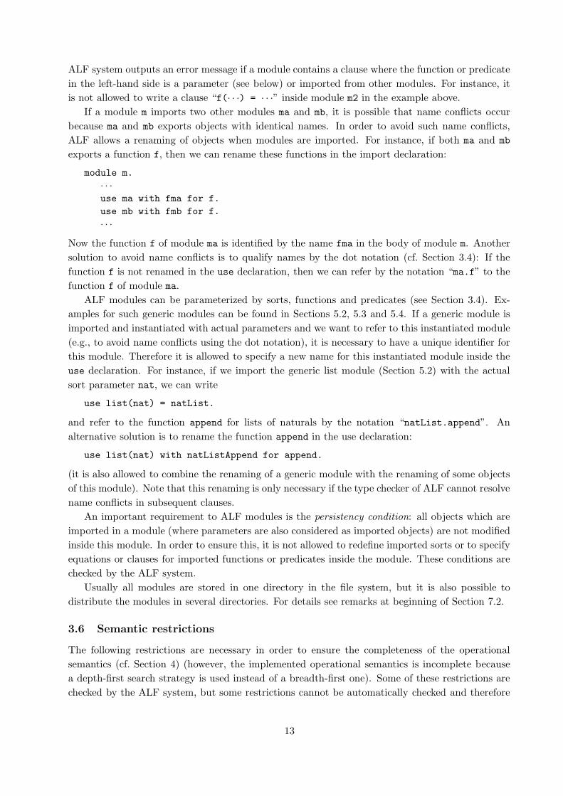
and innermost basic narrowing for functions. In order to give a precise definition of the operational
semantics, we represent a goal by a skeleton and an environment part [Hol88]: the skeleton is a
goal composed of terms and literals occurring in the original program, and the environment is a
substitution which has to be applied to the goal in order to obtain the current goal. The initial
goal G is represented by the pair < G; id > where id is the identity substitution. We define the
following inference rules to derive a new goal from a given one (if π is a position in a term t, then
t/π denotes the subterm of t at position π and t[π ← s] denotes the term obtained by replacing
the subterm t/π by s in t): Let < L1, . . . , Ln ; σ > be a given goal (L1, . . . , Ln are the skeleton
literals and σ is the environment).
1. If L1 is an equation s = t and there is a mgu σ ′ for σ(s) and σ(t), then the goal
< L2, . . . , Ln ; σ′ ◦ σ >
is derived by reflection.
2. If L1 is not an equation and there is a new variant L ← C of a program clause and σ ′ is a
mgu for σ(L1) and L, then the goal
< C,L2, . . . , Ln ; σ′ ◦ σ >
is derived by resolution.
3. Let π be a leftmost-innermost position in the first skeleton literal L1, i.e., the subterm L1/π
has a defined function symbol at the top and all argument terms consist of variables and
constructors (cf. [Fri85]).
(a) If there is a new variant l = r ← C of a program clause and σ(L1/π) and l are unifiable
with mgu σ′, then the goal
< C,L1[π ← r], L2, . . . , Ln ; σ′ ◦ σ >
is derived by innermost basic narrowing,
(b) If x is a new variable and σ′ is the substitution {x← σ(L1/π)}, then the goal
< L1[π ← x], L2, . . . , Ln ; σ′ ◦ σ >
is derived by innermost reflection (this corresponds to the elimination of an innermost
redex [Hol88]).
4. If π is a non-variable position in L1, l = r ← C is a new variant of a program clause and σ ′
is a substitution with σ(L1/π) = σ′(l) and the goal < C ; σ′ > can be derived to the empty
goal without instantiating any variables from σ(L1), then the goal
< L1[π ← σ′(r)], L2, . . . , Ln ; σ >
is derived by rewriting (thus rewriting is only applied to the first literal, but this
is no restriction since a conjunction like L1, L2, L3 can also be written as an equation
and(L1, and(L2, L3)) = true).
15
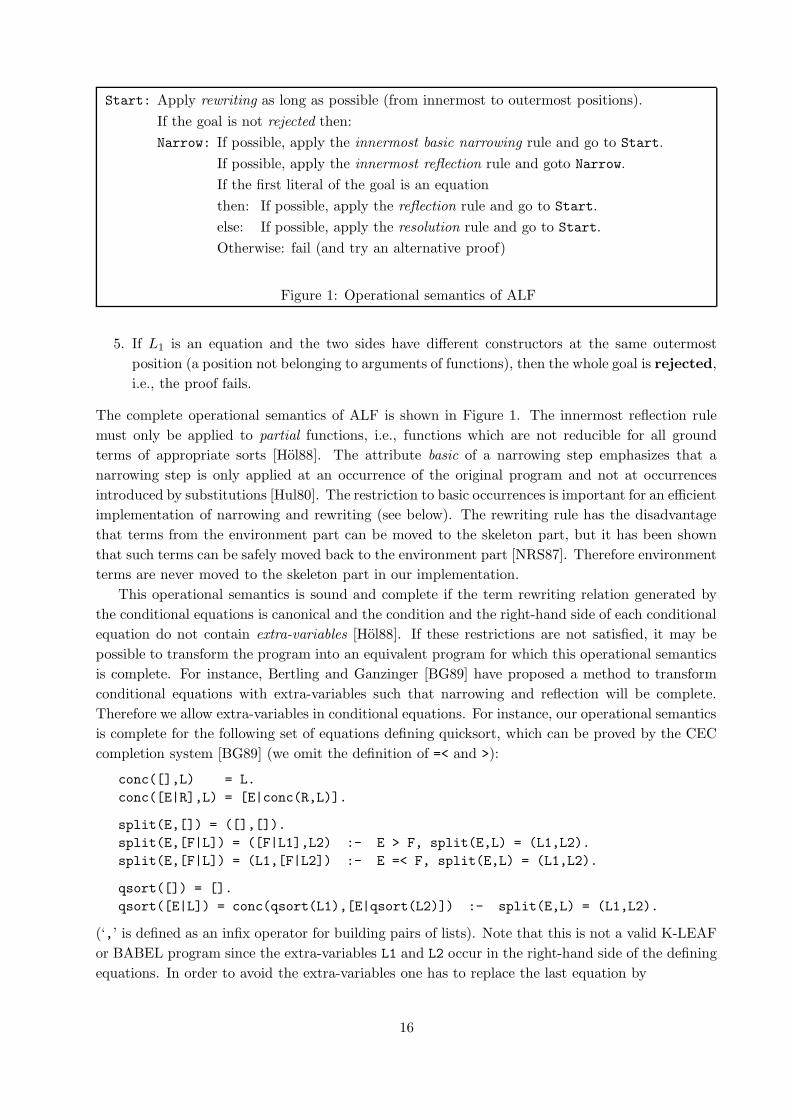
Start: Apply rewriting as long as possible (from innermost to outermost positions).
If the goal is not rejected then:
Narrow: If possible, apply the innermost basic narrowing rule and go to Start.
If possible, apply the innermost reflection rule and goto Narrow.
If the first literal of the goal is an equation
then: If possible, apply the reflection rule and go to Start.
else: If possible, apply the resolution rule and go to Start.
Otherwise: fail (and try an alternative proof)
Figure 1: Operational semantics of ALF
5. If L1 is an equation and the two sides have different constructors at the same outermost
position (a position not belonging to arguments of functions), then the whole goal is rejected,
i.e., the proof fails.
The complete operational semantics of ALF is shown in Figure 1. The innermost reflection rule
must only be applied to partial functions, i.e., functions which are not reducible for all ground
terms of appropriate sorts [Hol88]. The attribute basic of a narrowing step emphasizes that a
narrowing step is only applied at an occurrence of the original program and not at occurrences
introduced by substitutions [Hul80]. The restriction to basic occurrences is important for an efficient
implementation of narrowing and rewriting (see below). The rewriting rule has the disadvantage
that terms from the environment part can be moved to the skeleton part, but it has been shown
that such terms can be safely moved back to the environment part [NRS87]. Therefore environment
terms are never moved to the skeleton part in our implementation.
This operational semantics is sound and complete if the term rewriting relation generated by
the conditional equations is canonical and the condition and the right-hand side of each conditional
equation do not contain extra-variables [Hol88]. If these restrictions are not satisfied, it may be
possible to transform the program into an equivalent program for which this operational semantics
is complete. For instance, Bertling and Ganzinger [BG89] have proposed a method to transform
conditional equations with extra-variables such that narrowing and reflection will be complete.
Therefore we allow extra-variables in conditional equations. For instance, our operational semantics
is complete for the following set of equations defining quicksort, which can be proved by the CEC
completion system [BG89] (we omit the definition of =< and >):
conc([],L) = L.
conc([E|R],L) = [E|conc(R,L)].
split(E,[]) = ([],[]).
split(E,[F|L]) = ([F|L1],L2) :- E > F, split(E,L) = (L1,L2).
split(E,[F|L]) = (L1,[F|L2]) :- E =< F, split(E,L) = (L1,L2).
qsort([]) = [].
qsort([E|L]) = conc(qsort(L1),[E|qsort(L2)]) :- split(E,L) = (L1,L2).
(‘,’ is defined as an infix operator for building pairs of lists). Note that this is not a valid K-LEAF
or BABEL program since the extra-variables L1 and L2 occur in the right-hand side of the defining
equations. In order to avoid the extra-variables one has to replace the last equation by
16
qsort([E|L]) = conc(qsort(split1(E,L)),[E|qsort(split2(E,L))])
and redefine the split function. This solution is less efficient (because the list L must be processed
twice) and simplification orderings fail to prove the termination of the rewrite relation [BG89].
These drawbacks may be accepted, but there are other examples where the use of extra-variables
cannot be avoided with simple transformations. The function last computes the last element of
a given list. It can be explicitly defined or, if conc is defined as above, by the simple conditional
equation
last(L) = E :- conc(L1,[E]) = L.
In this case last(L) is evaluated by searching the right instantiations of L1 and E (note that there
is at most one solution if L is given). The use of extra-variables gives us the full power of logic
programming inside functional programming. Hence ALF allows extra-variables in conditional
equations. If such a conditional equation is applied in a rewrite step, only the first solution to the
extra-variables is considered. This is sufficient because all equations are required to be confluent.
It is also possible to specify additional equational clauses which are only used for rewriting. For
instance, Fribourg [Fri85] has shown that the addition of inductive axioms for rewriting is useful to
reduce the search space. In this case the proved goals are valid with respect to the least Herbrand
model but may be invalid in the class of all models. Therefore an ALF-program consists of three
groups of clauses:
1. Relational clauses which define all predicates except “=”.
2. Conditional equations used for narrowing.
3. Conditional equations used for rewriting.
Usually, all conditional equations in an ALF-program are used for narrowing and rewriting, but
the programmer can specify that some equations should only be applied for narrowing or rewriting,
respectively (this is the meaning of the suffix onlynarrow and onlyrewrite in equational rules).
For instance, the inductive axiom rev(rev(L)) = L can be used for rewriting to reduce the search
space (the function rev reverses all elements in a list). To use it as a narrowing rule makes no
sense since this would expand the search space.
Similarly to Prolog, the program clauses in ALF are ordered and the different choices for clauses
in a computation step are implemented by a backtracking strategy. Note that backtracking is only
necessary in the resolution and narrowing rule but not in rewriting since simplification by rewriting
produces unique terms independently of the chosen clauses (because of the confluence of the term
rewriting relation).
In order to demonstrate the improved efficiency of this operational semantics in comparison to
Prolog’s computation strategy, consider the following equations for the concatenation function on
lists:
conc([],L) = L
conc([E|R],L) = [E|conc(R,L)]
If a and b are constructors, then the goal
conc(conc([a|V],W),Y) = [b|Z]
is simplified by rewriting to the goal
[a|conc(conc(V,W),Y)] = [b|Z]
17
which is immediately rejected since a and b are different constructors. The equivalent Prolog goal
append([a|V],W,L), append(L,Y,[b|Z])
causes an infinite loop for any order of literals and clauses [Nai87]. More details about the ad-
vantages of rewriting and rejection in combination with narrowing can be found in [Fri85] and
[Han92].
5 Examples
In this section we present several examples for ALF programs and ALF modules defining basic
data types.
5.1 Natural numbers
Our first example is the definition of the basic ALF module nats defining natural numbers and
two functions and a predicate on naturals:
module nats.
export 0, s, + , *, < .
datatype nat = { 0 ; s(nat) }.
func + : nat, nat -> nat infixleft 500;
* : nat, nat -> nat infixleft 400.
pred < : nat, nat infix.
rules.
N + 0 = N.
0 + N = N onlyrewrite.
N + s(M) = s(N + M).
s(N) + M = s(N + M) onlyrewrite.
N * 0 = 0.
0 * N = 0 onlyrewrite.
N * s(M) = N + N * M.
s(M) * N = N + N * M onlyrewrite.
0 < s(_).
s(N) < s(M) :- N < M.
end nats.
Note that the commutative laws for addition and multiplication are only used for rewriting. Using
these rules also for narrowing would expand the search space. Since the onlyrewrite rules are
inductive consequences of the other rules, it is allowed to use such rules for rewriting if we are inter-
ested in answers valid w.r.t. the initial model (least Herbrand model). See [Fri85] for a discussion
of the use of additional rewrite rules.
5.2 Polymorphic lists
The next example is the basic module list which contains the definition of lists of elements of an
arbitrary type:
18
module list(elem).
export [] , ’.’ , append , length , member .
use nats.
datatype list = { ’.’(elem,list) ; [] }.
func append: list, list -> list;
length: list -> nat.
pred member : elem, list.
rules.
append([],L) = L.
append([H|T],L) = [H|append(T,L)].
length([]) = 0.
length([_|L]) = s(length(L)).
member(E,[E|_]).
member(E,[_|L]) :- member(E,L).
end list.
5.3 Stacks
The following module defines stacks of an arbitrary type. Note that the functions pop and top are
partial since they are not reducible on the argument term empty (cf. page 3.6):
module stackmod(elem).
export empty, push, top, pop, isEmpty, isNotEmpty.
datatype stack = { empty ; push(elem,stack) }.
func pop : stack -> stack partial;
top : stack -> elem partial.
pred isEmpty : stack;
isNotEmpty: stack.
rules.
pop(push(X,S)) = S.
top(push(X,S)) = X.
isEmpty(empty).
isNotEmpty(push(X,S)).
end stackmod.
5.4 A generic sort module
The following module contains a sort function on lists which is defined by the quicksort algorithm.
It is a generic module which has the sort of the list elements and a comparison predicate on these
elements as parameters:
module qsortpoly(elem, (pred lesseq: elem, elem)).
19

use list(elem).
func qsort : list -> list.
pred split : elem, list, list, list.
rules.
qsort([]) = [].
qsort([E|L]) = append(qsort(L1),[E|qsort(L2)]) :- split(E,L,L1,L2).
split(E,[],[],[]).
split(E,[E1|L],[E1|L1],L2) :- lesseq(E1,E), split(E,L,L1,L2).
split(E,[E2|L],L1,[E2|L2]) :- lesseq(E,E2), split(E,L,L1,L2).
end qsortpoly.
Note that the equations use the feature of extra variables of ALF (compare Section 4).
6 Predefined functions and predicates
The current implementation of ALF has several functions and predicates which cannot be defined
by Horn clauses but have a fixed interpretation with some side effects during the evaluation. Such
functions and predicates are called predefined. The type definitions of these objects are contained
in the modules string, term, operator, streamio and system. This section shows the declaration
part of these modules (without export and use declarations) and gives an informal description of
the definitions.
If the predefined functions and predicates require some arguments, then these arguments must
be bound to ground terms when the function or predicate is evaluated. Otherwise an error will be
reported.
6.1 The module string
module string.
datatype string.
use list(string) with stringList for list.
func conc_string : string, string -> string.
pred string_nat : string, nat;
string_chars : string, stringList;
compare_string: string, string.
...
Figure 2: Module string
The module string (Figure 2) contains the necessary definitions to use string constants in ALF
programs. A sequence of characters enclosed in double quotes is a term (constant) of type string.
This module defines the sort string and operations on this builtin type.
The function conc_string returns the concatenation of the argument strings. E.g.,
conc_string("ab","cd") will be evaluated to the constant term "abcd".
20
The predicate string_nat compares a natural number with its string representation and is
used to convert a string into a natural number and vice versa. If the first argument of a call to
string_nat is a string representation of a natural number, then the value of the natural number
(represented in ALF by an s-term, cf. Section 5.1) is unified with the second argument. If the first
argument is a string which is not a valid representation of a natural number, then the predicate
call fails. If the second argument is the ALF representation of a natural number (cf. Section 5.1),
then a string representing this number is generated and unified with the first argument. E.g.,
string_nat("3",s(s(s(0)))) is provable, but string_nat("ab",N) fails.
The predicate string_chars can be used to decompose a string into its characters or to con-
catenate a list of strings into a single string. If the second argument of a call to string_chars
is a list of strings, then these strings are concatenated and the resulting string is unified with
the first argument. If the second argument is an unbound variable, then the first argument must
be a string which will be decomposed into its list of characters (where each character is repre-
sented by a string of length 1) and then the second argument will be bound to this list. For
instance, a call of string_chars(S,["ab","cde"]) binds S to the string "abcde", and a call of
string_chars("abc",L) binds L to the list ["a","b","c"]. Note that if the second argument
is not an unbound variable when calling string_chars, then it must be a list of strings (without
variables), otherwise a run-time error will occur.
The predicate compare_string compares two strings. The literal compare_string(S,T)
is provable iff string S is less than string T in lexicographic order. For instance,
compare_string("alf","alfcompile") is provable while compare_string("beta","alpha")
fails.
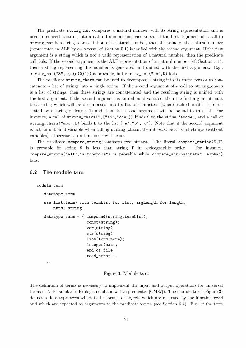
6.2 The module term
module term.
datatype term.
use list(term) with termList for list, argLength for length;
nats; string.
datatype term = { compound(string,termList);
const(string);
var(string);
str(string);
list(term,term);
integer(nat);
end_of_file;
read_error }....
Figure 3: Module term
The definition of terms is necessary to implement the input and output operations for universal
terms in ALF (similar to Prolog’s read and write predicates [CM87]). The module term (Figure 3)
defines a data type term which is the format of objects which are returned by the function read
and which are expected as arguments to the predicate write (see Section 6.4). E.g., if the term
21

“f(g(X),1).” is on the input stream, the function read returns the ALF term
compound("f",[compound("g",[var("X")]),integer(s(0))])
The meaning of the individual constructors of sort term are:
compound represents a structured term where the first argument is the functor of the term
and the second argument is the list of arguments of the structure. For instance,
compound("f",[const("a"),const("b")]) represents the term “f(a,b)”.
const represents an atomic constant where the argument is the name of the atom. For instance,
const("alf") and const("ALF") represent the atoms “alf” and “’ALF’”, respectively. Note
that atoms beginning with an upper-case character must always be quoted, otherwise they
will be interpreted as a variable.
var represents a variable where the argument is the name of the variable. For instance, the variable
“List” is represented by the term var("List").
str represents a string which is a sequence of characters enclosed in double quotes (cf. Section 6.1).
For instance, the string constant “"a string"” is represented by str("a string").
list represents a list which is written using the list notation (see Section 3.3). The first argument
is the first element of the list and the second argument is the rest of the list. For instance, the
list “[a]” is represented by list(const("a"),const("[]")). Note that a binary structure
with the functor “.” is not represented as a list, i.e., the term “.(a,b)” is represented by
compound(".",[const("a"),const("b")]).
integer is the represenation of an integer constant where the argument is the value of the constant.
For instance, “2” is represented by integer(s(s(0))).
end_of_file is a special object which is returned by read if the input stream has ended.
read_error is another special object which is returned by read if a syntax error has occurred
while reading the input stream.
6.3 The module operator
module operator.
datatype operator = { (infixleft(string,nat) infixnot 650) ;
(infixright(string,nat) infixnot 650) ;
(infixnot(string,nat) infixnot 650) ;
(prefix(string,nat) infixnot 650) ;
(postfix(string,nat) infixnot 650) ;
nonop }.
use list(operator) with operatorList for list, opListMember for member.
...
Figure 4: Module operator
In order to allow a flexible syntax with operator definitions (similar to Prolog [CM87]) as input
to the predefined function read, it is necessary to declare operator tables which are parameters
22
to read. Hence the read function assumes that one parameter is a list of operator declarations
which are terms of type operator w.r.t. module operator (Figure 4). The constructors infixleft,
infixright, infixnot, prefix and postfix are infix operators which construct the elements of a
list of type operatorList. For instance,
["+" infixleft 500, "+" prefix 500, "*" infixleft 400]
is an operator table where the atom + is an infix and a prefix operator and * is an infix operator.
The precedence of * is lower than the precedence of + which means that a term of the form 1+2*3
is interpreted as 1+(2*3).
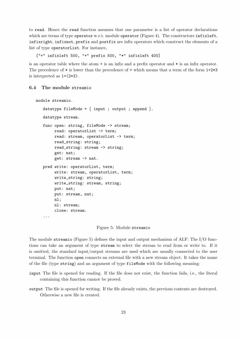
6.4 The module streamio
module streamio.
datatype fileMode = { input ; output ; append }.
datatype stream.
func open: string, fileMode -> stream;
read: operatorList -> term;
read: stream, operatorList -> term;
read_string: string;
read_string: stream -> string;
get: nat;
get: stream -> nat.
pred write: operatorList, term;
write: stream, operatorList, term;
write_string: string;
write_string: stream, string;
put: nat;
put: stream, nat;
nl;
nl: stream;
close: stream.
...
Figure 5: Module streamio
The module streamio (Figure 5) defines the input and output mechanism of ALF: The I/O func-
tions can take an argument of type stream to select the stream to read from or write to. If it
is omitted, the standard input/output streams are used which are usually connected to the user
terminal. The function open connects an external file with a new stream object. It takes the name
of the file (type string) and an argument of type fileMode with the following meaning:
input The file is opened for reading. If the file does not exist, the function fails, i.e., the literal
containing this function cannot be proved.
output The file is opened for writing. If the file already exists, the previous contents are destroyed.
Otherwise a new file is created.
23
append The file is opened for writing. The previous contents of an existing file are not destroyed,
but the new items are appended to the file. If the file does not exist, a new file is created.
A call to the predicate close closes the stream.
The argument of read and write of type operatorList is a list of operator definitions (see
Section 6.3). The function read reads a term according to these operator definitions from the
input stream and returns the corresponding object of type term (see Section 6.2) as the result.
The predicate write prints an object of type term according to the operator list parameter on the
output stream.
read_string and write_string are used to read and write precisely one string. The func-
tion read_string reads a line from the input stream and returns this line (without the line feed
character) as a string. The predicate write_string prints a single string on the output stream.
It is also possible to get and put single characters. The function get reads the next character
from the input stream and returns the corresponding ASCII value of this character. The predicate
put writes the character with the ASCII value of the argument to the output stream. nl is
equivalent to put(10), i.e., nl puts a newline character on the output stream.
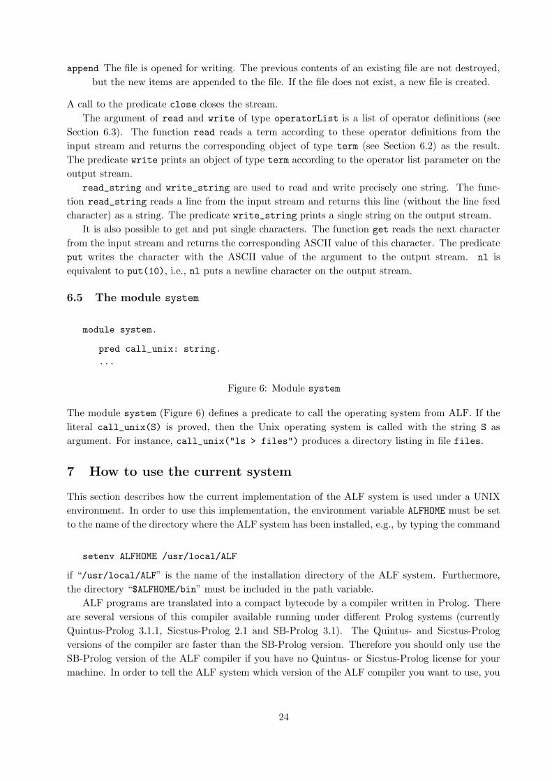
6.5 The module system
module system.
pred call_unix: string.
...
Figure 6: Module system
The module system (Figure 6) defines a predicate to call the operating system from ALF. If the
literal call_unix(S) is proved, then the Unix operating system is called with the string S as
argument. For instance, call_unix("ls > files") produces a directory listing in file files.
7 How to use the current system
This section describes how the current implementation of the ALF system is used under a UNIX
environment. In order to use this implementation, the environment variable ALFHOME must be set
to the name of the directory where the ALF system has been installed, e.g., by typing the command
setenv ALFHOME /usr/local/ALF
if “/usr/local/ALF” is the name of the installation directory of the ALF system. Furthermore,
the directory “$ALFHOME/bin” must be included in the path variable.
ALF programs are translated into a compact bytecode by a compiler written in Prolog. There
are several versions of this compiler available running under different Prolog systems (currently
Quintus-Prolog 3.1.1, Sicstus-Prolog 2.1 and SB-Prolog 3.1). The Quintus- and Sicstus-Prolog
versions of the compiler are faster than the SB-Prolog version. Therefore you should only use the
SB-Prolog version of the ALF compiler if you have no Quintus- or Sicstus-Prolog license for your
machine. In order to tell the ALF system which version of the ALF compiler you want to use, you
24
must set the environment variable ALFPROLOG to an appropriate value i.e., you have to include one
of the commands
setenv ALFPROLOG quintus # for the Quintus-Prolog version
setenv ALFPROLOG sicstus # for the Sicstus-Prolog version
setenv ALFPROLOG sbprolog # for the SB-Prolog version
in your .cshrc-file. Ask the person who has installed the ALF system at your site for the ALF
compiler versions which are available on your machine.
7.1 Files
An ALF program is a collection of modules. Each module must be stored in a separate file. The
file with the main module contains also one or more goals at the end which should be proved by
the ALF system. Usually, the main module together with the goal and all imported modules is
compiled by the ALF system into a compact bytecode which will be executed by an emulator. The
compilation is divided into the following steps:
1. In the first step the main module and all imported modules are checked for syntactic errors
and type consistence. The result of the first step is a program where all types are deleted
and all modules are copied into one large program, the so-called “flat-ALF” program.
2. In the second step the flat-ALF program is translated into a sequence of instructions of
an abstract machine tailored for executing such programs very efficiently. The machine is
called A-WAM (since it is an extension of the Warren Abstract Machine for executing ALF
programs).
3. In the last step the A-WAM instructions are translated into a compact bytecode representing
the compiled ALF program. This bytecode is the input to the A-WAM emulator.
It is possible to compile ALF programs in one step into the bytecode or also in several separate
steps. Therefore the different versions of a program are distinguished by the following file name
suffixes:
.alf Files containing ALF modules. Module m must be stored in the file “m.alf”. At the end of
the main module the goals to be proved are appended.
.fal Files containing flat-ALF programs. The flat-ALF program corresponding to the main module
m (and all imported modules) is stored in the file “m.fal”.
.sow Files containing A-WAM programs. Hence “m.sow” contains a compiled version of the flat-
ALF program in “m.fal”.
.byt Files containing bytecodes of A-WAM programs. Thus the ALF program with main module
m is compiled into the bytecode stored in “m.byt”.
7.2 Compiling ALF programs
All modules modules of an ALF program must be stored in the directory where the ALF system is
called (the current directory) or in the global module directory “$ALFHOME/modules”. If a module
is imported, the corresponding file is searched in the current directory and then, if not found,
in the global module directory. Usually, the global module directory contains frequently used
25
and predefined modules like nats (page 18), list (page 18), string (page 20), term (page 21),
operator (page 22), streamio (page 23), and system (page 24).
It is also possible to import a module which is stored in another directory. In this case the
module name must be prefixed by the path name. Note that a module name in a use declaration
must always be an atom. Therefore the module name must be quoted if it is prefixed by the
path name. For instance, the module defaults in the directory /usr/lib/ALF is imported by the
following use declaration:
use ’/usr/lib/ALF/defaults’.
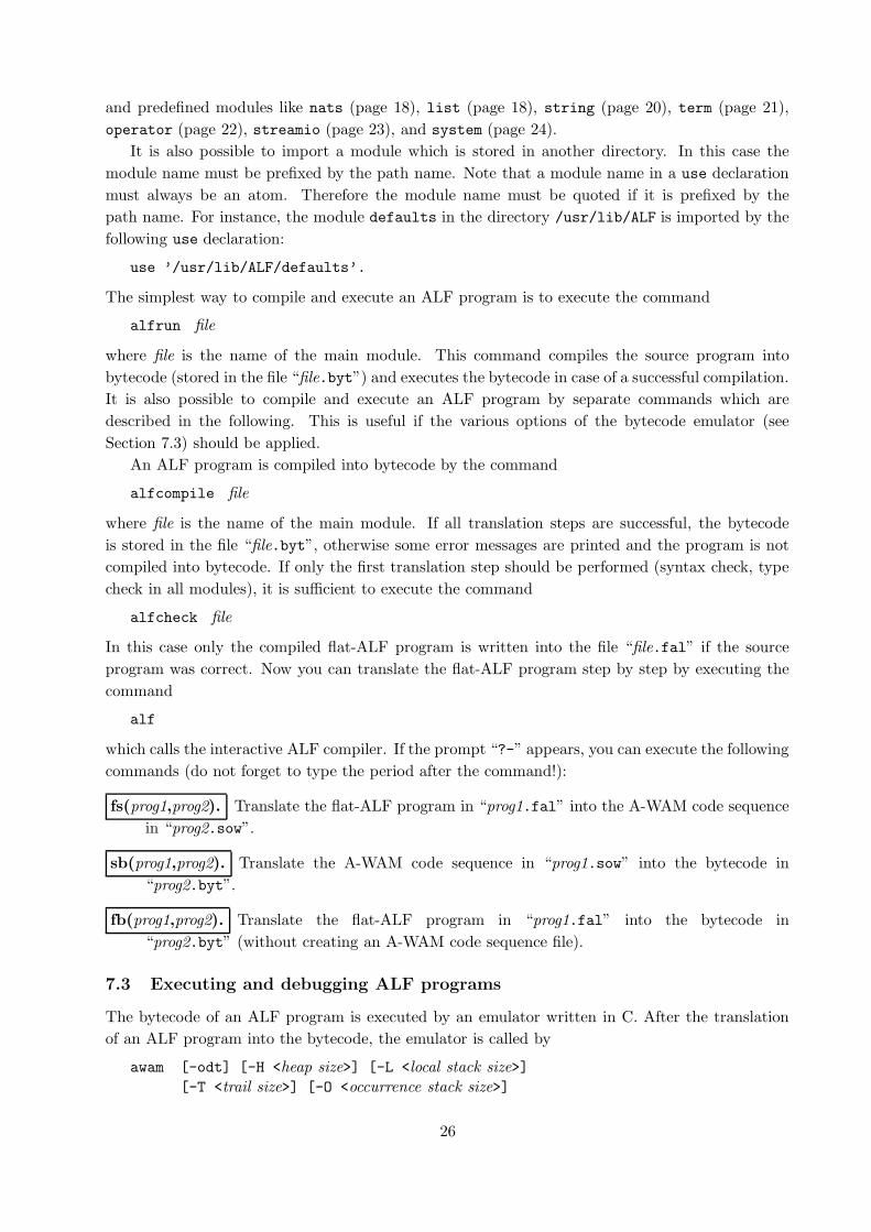
The simplest way to compile and execute an ALF program is to execute the command
alfrun file
where file is the name of the main module. This command compiles the source program into
bytecode (stored in the file “file.byt”) and executes the bytecode in case of a successful compilation.
It is also possible to compile and execute an ALF program by separate commands which are
described in the following. This is useful if the various options of the bytecode emulator (see
Section 7.3) should be applied.
An ALF program is compiled into bytecode by the command
alfcompile file
where file is the name of the main module. If all translation steps are successful, the bytecode
is stored in the file “file.byt”, otherwise some error messages are printed and the program is not
compiled into bytecode. If only the first translation step should be performed (syntax check, type
check in all modules), it is sufficient to execute the command
alfcheck file
In this case only the compiled flat-ALF program is written into the file “file.fal” if the source
program was correct. Now you can translate the flat-ALF program step by step by executing the
command
alf
which calls the interactive ALF compiler. If the prompt “?-” appears, you can execute the following
commands (do not forget to type the period after the command!):
fs(prog1,prog2). Translate the flat-ALF program in “prog1.fal” into the A-WAM code sequence
in “prog2.sow”.
sb(prog1,prog2). Translate the A-WAM code sequence in “prog1.sow” into the bytecode in
“prog2.byt”.
fb(prog1,prog2). Translate the flat-ALF program in “prog1.fal” into the bytecode in
“prog2.byt” (without creating an A-WAM code sequence file).
7.3 Executing and debugging ALF programs
The bytecode of an ALF program is executed by an emulator written in C. After the translation
of an ALF program into the bytecode, the emulator is called by
awam [-odt] [-H <heap size>] [-L <local stack size>][-T <trail size>] [-O <occurrence stack size>]
26

[--occur-check] [--debug] [--trace]
[--heap-size=<heap size>] [--ls-size=<local stack size>][--trail-size=<trail size>][--occ-size=<occurrence stack size>]filename[.byt]
where the following options are equivalent:
-o = --occur-check
-d = --debug
-t = --trace
There is also a statistical version of the A-WAM emulator which is executed by calling awamS instead
of awam. If the awamS emulator is terminated, statistics about the used memory are printed.
The options have the following meaning (the last argument is always the name of the bytecode
file):
occur-check Unification is performed with occur check. Without this option the A-WAM does
not perform an occur check.
debug The emulator executes the bytecode in debug mode (see below).
trace The emulator executes the bytecode in trace mode, i.e., all executed A-WAM instructions
are printed on the standard output stream.
heap-size Set the heap size to the given number of bytes (default: 2 Mbytes). If an execution
stops with the error message “Heap overflow”, restart the emulator with a larger heap size.
ls-size Set the local stack size to the given number of bytes (default: 2 Mbytes). If an execution
stops with the error message “Local-Stack overflow”, restart the emulator with a larger local
stack size.
trail-size Set the trail size to the given number of bytes (default: 400 Kbytes). If an execution
stops with the error message “Trail overflow”, restart the emulator with a larger trail size.
occ-size Set the occurrence stack size to the given number of bytes (default: 200 Kbytes). If an
execution stops with the error message “Occurrence-Stack overflow”, restart the emulator
with a larger occurrence stack size.
In the standard mode the emulator computes a solution to the first given goal by interpreting the
A-WAM instructions. If a solution is found, the instantiated goal is written on the standard output
and the emulator waits for an input. If the input is empty, the emulator is terminated. If the input
is “;”, the next solution is computed or the next goal is solved (if there is no alternative solution
to the current goal).
In the trace mode the emulator prints all executed A-WAM instructions on the standard output
stream.
In the debug mode the emulator stops at particular A-WAM instructions which corresponds
to the evaluation of a function or predicate. Hence a behaviour similarly to the common Prolog
debuggers is obtained. If a predicate is called, the emulator prints the string CALL together with the
currently called predicate (with instantiated argument terms). If a function should be evaluated
by rewriting, the emulator prints the string REWRITE together with the current function call. If a
27
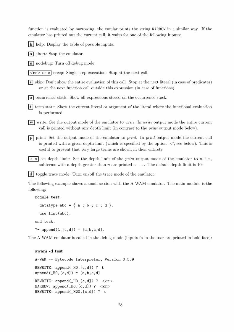
function is evaluated by narrowing, the emular prints the string NARROW in a similar way. If the
emulator has printed out the current call, it waits for one of the following inputs:
h help: Display the table of possible inputs.
a abort: Stop the emulator.
n nodebug: Turn off debug mode.
<cr> or c creep: Single-step execution: Stop at the next call.
s skip: Don’t show the entire evaluation of this call. Stop at the next literal (in case of predicates)
or at the next function call outside this expression (in case of functions).
o occurrence stack: Show all expressions stored on the occurrence stack.
t term start: Show the current literal or argument of the literal where the functional evaluation
is performed.
w write: Set the output mode of the emulator to write. In write output mode the entire current
call is printed without any depth limit (in contrast to the print output mode below).
p print: Set the output mode of the emulator to print. In print output mode the current call
is printed with a given depth limit (which is specified by the option ’<’, see below). This is
useful to prevent that very large terms are shown in their entirety.
< n set depth limit: Set the depth limit of the print output mode of the emulator to n, i.e.,
subterms with a depth greater than n are printed as ... The default depth limit is 10.
d toggle trace mode: Turn on/off the trace mode of the emulator.
The following example shows a small session with the A-WAM emulator. The main module is the
following:
module test.
datatype abc = { a ; b ; c ; d }.
use list(abc).
end test.
?- append(L,[c,d]) = [a,b,c,d].
The A-WAM emulator is called in the debug mode (inputs from the user are printed in bold face):
awam -d test
A-WAM -- Bytecode Interpreter, Version 0.5.9
REWRITE: append(_H0,[c,d]) ? tappend(_H0,[c,d]) = [a,b,c,d]
REWRITE: append(_H0,[c,d]) ? <cr>NARROW: append(_H0,[c,d]) ? <cr>REWRITE: append(_H20,[c,d]) ? t
28
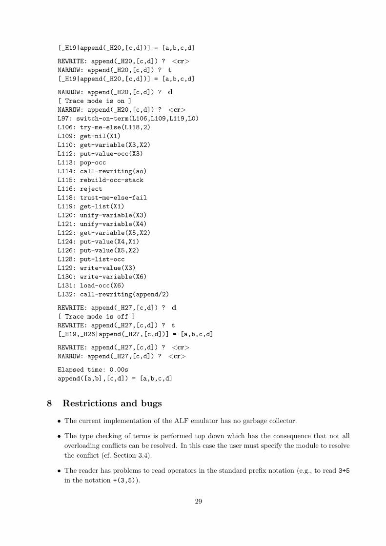
[_H19|append(_H20,[c,d])] = [a,b,c,d]
REWRITE: append(_H20,[c,d]) ? <cr>NARROW: append(_H20,[c,d]) ? t[_H19|append(_H20,[c,d])] = [a,b,c,d]
NARROW: append(_H20,[c,d]) ? d[ Trace mode is on ]
NARROW: append(_H20,[c,d]) ? <cr>L97: switch-on-term(L106,L109,L119,L0)
L106: try-me-else(L118,2)
L109: get-nil(X1)
L110: get-variable(X3,X2)
L112: put-value-occ(X3)
L113: pop-occ
L114: call-rewriting(ao)
L115: rebuild-occ-stack
L116: reject
L118: trust-me-else-fail
L119: get-list(X1)
L120: unify-variable(X3)
L121: unify-variable(X4)
L122: get-variable(X5,X2)
L124: put-value(X4,X1)
L126: put-value(X5,X2)
L128: put-list-occ
L129: write-value(X3)
L130: write-variable(X6)
L131: load-occ(X6)
L132: call-rewriting(append/2)
REWRITE: append(_H27,[c,d]) ? d[ Trace mode is off ]
REWRITE: append(_H27,[c,d]) ? t[_H19,_H26|append(_H27,[c,d])] = [a,b,c,d]
REWRITE: append(_H27,[c,d]) ? <cr>NARROW: append(_H27,[c,d]) ? <cr>
Elapsed time: 0.00s
append([a,b],[c,d]) = [a,b,c,d]
8 Restrictions and bugs
• The current implementation of the ALF emulator has no garbage collector.
• The type checking of terms is performed top down which has the consequence that not all
overloading conflicts can be resolved. In this case the user must specify the module to resolve
the conflict (cf. Section 3.4).
• The reader has problems to read operators in the standard prefix notation (e.g., to read 3+5
in the notation +(3,5)).
29
References
[BG89] H. Bertling and H. Ganzinger. Completion-Time Optimization of Rewrite-Time GoalSolving. In Proc. of the Conference on Rewriting Techniques and Applications, pp. 45–58.Springer LNCS 355, 1989.
[CM87] W.F. Clocksin and C.S. Mellish. Programming in Prolog. Springer, third rev. and ext.edition, 1987.
[Fri85] L. Fribourg. SLOG: A Logic Programming Language Interpreter Based on Clausal Su-perposition and Rewriting. In Proc. IEEE Internat. Symposium on Logic Programming,pp. 172–184, Boston, 1985.
[GM86] E. Giovannetti and C. Moiso. A completeness result for E-unification algorithms basedon conditional narrowing. In Proc. Workshop on Foundations of Logic and FunctionalProgramming, pp. 157–167. Springer LNCS 306, 1986.
[Han90] M. Hanus. Compiling Logic Programs with Equality. In Proc. of the 2nd Int. Workshop onProgramming Language Implementation and Logic Programming, pp. 387–401. SpringerLNCS 456, 1990.
[Han91] M. Hanus. Efficient Implementation of Narrowing and Rewriting. In Proc. Int. Workshopon Processing Declarative Knowledge, pp. 344–365. Springer LNAI 567, 1991.
[Han92] M. Hanus. Improving Control of Logic Programs by Using Functional Logic Languages.In Proc. of the 4th International Symposium on Programming Language Implementationand Logic Programming, pp. 1–23. Springer LNCS 631, 1992.
[Hol88] S. Holldobler. From Paramodulation to Narrowing. In Proc. 5th Conference on LogicProgramming & 5th Symposium on Logic Programming (Seattle), pp. 327–342, 1988.
[Hul80] J.-M. Hullot. Canonical Forms and Unification. In Proc. 5th Conference on AutomatedDeduction, pp. 318–334. Springer LNCS 87, 1980.
[MH92] A. Middeldorp and E. Hamoen. Counterexamples to Completeness Results for Basic Nar-rowing. In Proc. of the 3rd International Conference on Algebraic and Logic Programming,pp. 244–258. Springer LNCS 632, 1992.
[Nai87] L. Naish. Negation and Control in Prolog. Springer LNCS 238, 1987.
[NRS87] W. Nutt, P. Rety, and G. Smolka. Basic Narrowing Revisited. SEKI Report SR-87-07,FB Informatik, Univ. Kaiserslautern, 1987.
[Pad88] P. Padawitz. Computing in Horn Clause Theories, volume 16 of EATCS Monographs onTheoretical Computer Science. Springer, 1988.
[War83] D.H.D. Warren. An Abstract Prolog Instruction Set. Technical Note 309, SRI Interna-tional, Stanford, 1983.
30


![Curry: An Integrated Functional Logic Languageantoy/Courses/TPFLP/report.pdf · Curry An Integrated Functional Logic Language Version 0.9.0 January 13, 2016 Michael Hanus1 [editor]](https://img.dokumen.tips/doc/110x75/608871a801c345296e5cc855/curry-an-integrated-functional-logic-language-antoycoursestpflp-curry-an.jpg)