ALEX CE ZHANG 1 YU-HWA LO1*

Non-invasive optical measurement of arterialblood flow speed

ALEX CE ZHANG,1 YU-HWA LO1*

1Department of Electrical and Computer Engineering, University of California San Diego, 9500 GilmanDriver, La Jolla ,CA, 92092, USA*[email protected]

Abstract: Non-invasive measurement of the arterial blood speed gives rise to important healthinformation such as cardio output and blood supplies to vital organs. The magnitude andchange in arterial blood speed are key indicators of the health conditions and development andprogression of diseases. We demonstrated a simple technique to directly measure the blood flowspeed in main arteries based on the diffused light model. The concept is demonstrated with aphantom that uses intralipid hydrogel to model the biological tissue and an embedded glass tubewith flowing human blood to model the blood vessel. The correlation function of the measuredphotocurrent was used to find the electrical field correlation function via the Siegert relation.We have shown that the characteristic decorrelation rate (i.e. the inverse of the decoherent time)is linearly proportional to the blood speed and independent of the tube diameter. This strikingproperty can be explained by an approximate analytic solution for the diffused light equation inthe regime where the convective flow is the dominating factor for decorrelation. As a result, wehave demonstrated a non-invasive method of measuring arterial blood speed without any priorknowledge or assumption about the geometric or mechanic properties of the blood vessels.

1. Introduction

Oxygenated red blood cells in the blood flow deliver essential nutrients and oxygen to organs andlimbs to maintain their homeostatic conditions and proper functions. Oximeter detects the oxygensaturation level of red blood cells by using wavelength dependent absorption for oxygenated anddeoxygenated blood [1]. Such measurements can be done with wearable devices such as smartwatches. On the other hand, there has been no convenient and non-invasive method to measurethe amount of blood supply or blood speed in major arteries.

Reduced blood supply is usually a sign of diseases and medical conditions. Dehydration,thromboses formation, and other physiological and pathological conditions can cause short termor long term changes in the blood speed at a given location of the artery [2]. The informationhelps early diagnosis and monitoring of diseases with impaired blood flow [3–5]. Therefore, it isdesirable to directly measure the travelling velocity of red blood cells at well-defined locationssuch as the carotidal artery to the head, femoral artery to the lower limb, brachial artery to theupper arm, spinal arteries to the spinal cord, renal arteries to the kidneys, hepatic artery to theliver, and pulmonary artery to the lungs, etc. Since the arterial blood speed at the well-definedpositions provide direct and unambiguous information about blood supply to the sites of healthconcerns.

Doppler frequency shift of ultrasonic waves offers a non-invasive measurement of the bloodflow speed at the well-defined position. However, acoustic measurements require close physicalcontacts of the ultrasound transducers with the tissue to allow efficient coupling of the acousticwave, and gel is needed to assure the quality and reliability of the contact. Furthermore, themeasured signal is highly dependent on the angle between the probe and the blood flow direction.The most convenient and ergonomic direction is to have the transducer perpendicular to theblood vessel. However, this arrangement will produce no Doppler shift signal, thus makingthe measurement less convenient in a homecare or nursing home setting for self-administeredoperation [6]. In this regard, an optical method is potentially more desirable because a light wave

arX

iv:2

110.

1040

8v1

[ph

ysic

s.m

ed-p

h] 2

0 O

ct 2

021

can enter the tissue via free space coupling and once entering the tissue, as we will discuss later,it travels diffusively. In addition, the optical hardware including semiconductor light sourcesand detectors are more compact than acoustic transmitters and receivers. People have useddynamic scattering of laser light by red blood cells to measure the speed for blood vessels nearthe tissue surface [7, 8]. Similar to the Doppler effect of sound propagation, the frequency of thescattered light by moving particles is also shifted. Although the operation principle seems to bestraightforward, the physical model of the “optical Doppler device” is based on a key assumptionthat the light is only scattered once by a moving object (e.g. a traveling red blood cell) and the restof the scatterings is produced by quasi static objects such as skin and fat. This assumption may bereasonable for probing near surface tissue blood flow, but not for major arteries where around 40%of the volume of the blood vessel with a diameter of a few millimeters is occupied by traveling redblood cells. Under the approximation of single light scattering by moving particles, the detectedscattered light will display a frequency shift proportional to the velocity of the particle and theamount of frequency shift can be detected using the homodyne coherent detection technique.However, the above technique cannot be applied to multiple scatterings by a large number ofmoving particles. In such situations, the frequency spectrum of the light wave is broadened,making the interpretation of signal difficult. Because of this limit, the current technique ofoptical Doppler shift has been limited to measuring the blood flow in microflow channels nearthe skin although the blood supply by major arteries produces more valuable information forhealth and disease conditions. In addition, the laser Doppler flowmetry can only measure relativespeed. [9]. To measure the blood flow speed in major arteries, we extend the technique of opticalscattering method by taking into account the effect of multiple scattering by red blood cells.Instead of measuring the Doppler shift in the optical frequency, we measure the decorrelationtime of the reflected light. The key results of our work are (a) we have shown experimentally andtheoretically that one can measure the arterial blood flow velocity using a simple optical setupcomprised of a single semiconductor laser and a single detector, both coupled to a multi-modefiber bundle, and (b) we discovered that for main arteries where the diffused light model applies,the decorrelation time is inversely proportional to the RBC speed and we can measure its valuewithout any prior knowledge about the anatomy and tissue mechanic properties of the artery.Once entering the tissue, light has a very short scattering mean free path and the light becomesdiffusive. Modelling of light propagation in this regime has led to the development of oximeterback in 70s [10] and many researchers have utilized the diffused light to construct images throughhighly diffusive biological media, such as reconstructed breast cancer images [11]. The standardconfiguration for diffused light correlation spectroscopy includes a point source and a pointdetector, and the measured correlation function depends on the relative position between thesource and the detector [12–14]. The method of diffused light correlation spectroscopy has beenused in blood perfusion measurement [15], including brain circulations [16–18]. The setup usesa single-mode fiber coupled detector to allow single-mode transmission of two orthogonal lightpolarizations [19]. The single spatial mode yields the best signal-to-noise ratio since it detectsone speckle. However, this setup produces very low light intensity and requires a single photondetector (e.g. a single-photon avalanche detector (SPAD) or a photomultiplier tube (PMT)),making the setup quite sophisticated and subject to interference and stray light.

To make the system robust and easy to operate, in this paper we use multimode fiber and aregular photodetector to detect temporal fluctuations of the light intensity. In the following wefirst present our experimental setup and measurement results, and then describe the physicalmodel to show how the measured results can be used to find the red blood cell velocity. Wewill show that in a simple and robust setup that is relatively insensitive to the optical alignmentbetween the fiber bundle and the tissue, where we can reliably measure the absolute value of thetraveling speed of red blood cells in a blood vessel that has a millimeter diameter embedded in alayer of tissue. The results offer a promising solution for non-invasive measurement of the blood

supply into organs and limbs.

2. Experimental Setup

The experimental setup and measured results are first presented here, followed by the theoreticalanalysis in the later sections.

Fig. 1. . Experimental Setup. The laser light illuminates the tissue phantom surface ata 45-degree angle and the scattered diffused light is collected through the reflectionprobe fiber bundle which is coupled to a photoreceiver. The glass tube that emulates ablood vessel is embedded in the tissue phantom 5mm below the surface.

2.1. Tissue Phantom Fabrication

Wwe used intralipid as the scattering agent to reproduce keymimic the tissue by making its opticalproperties of tissue to make the scattering coefficient `𝑠 and anisotropy factor 𝑔 similar to the thevalues of real tissue. Because of its similar optical properties to the bilipid membrane of cells,intralipid is commonly used to simulate tissue scattering [20–22]. In addition, the absorptioncoefficient of intralipid is low and its refractive index is close to that of soft tissue [23]. Thetissue phantom is created using intralipid (Sigma-Aldrich 20%) in gelatin gel. One percentconcentration of intralipid was chosen to achieve a scattering coefficient of around 10𝑐𝑚−1 at784 𝑛𝑚. The phantom was initially prepared at 90◦𝐶, and then poured into a mold where a glasstube was pre-inserted at a depth of 5mm from the phantom surface (measured from the center ofthe tube).The liquid phantom was immediately placed into a freezer at -18 ◦𝐶 for 30 minutes forrapid solidification to prevent sedimentation of intralipid to achieve a uniform scattering property.Then the sample was placed in a refrigerator at 6 ◦𝐶 for 30 minutes to further solidify. Thesubsequent experiment was usually completed within 30 minutes after the phantom fabrication toprevent evaporation induced dehydration of the phantom, which could reduce the surface height.Glass tubes of three different inner diameters were used to mimic the arteries. Tygon tubing wasconnected to both ends of the glass tube, with one end connected to a 10𝑚𝐿 syringe mounted ona syringe pump and the other end connected to a reservoir (See figure 1).

2.2. Blood Preparation

12 𝑚𝐿 of human whole blood collected on the same day of the experiment was purchased fromthe San Diego Blood Bank. EDTA was added to the blood sample to prevent coagulation.

2.3. Optical and electronics setup

We used an off-the-shelf multi-core reflection fiber bundle probe (Model:RP21 from Thorlabs)that consists of one center core surrounded by 6 peripheral cores to couple the input and reflectedlight. The center core was used to deliver the laser light to the blood vessel and the 6 peripheralcores that are merged into a single output are coupled to the photodetector (see Fig. 1). The fiberbundle was mounted about 45 degrees relative to the surface of the tissue phantom to preventspecular refection from the tissue surface. The fiber bundle was coarsely aligned to the positionof the glass tube in the tissue phantom. The laser used in the experiment was an off-the-shelf fibercoupled laser diode at 785nm, biased slightly above its threshold current to produce an outputof 5 mW. The output of the detection fiber was coupled to a silicon APD with an integratedtransimpedance amplifier (Thorlabs APD410A) to achieve a transimpedance gain of 500 kV/Aat 10MHz bandwidth. The APD multiplication gain was set to be the lowest (𝑀 ∼ 10). Theoutput signal from the APD photoreceiver entered a data acquisition board (Advantech PCI-E1840) at a sampling rate of 20 Msps, yielding a Nyquist bandwidth of 10 MHz. The total dataacquisition time for the measurement was 25 seconds. We treated each 5ms duration as onerecording section, so 25 seconds of measurement produced 5,000 sections for analysis and noisecancellation. In all the data presented next, we used the average data over 25 seconds for themean and over 1 second to determine the variations shown in error bars.

We tested blood flows with three tube inner diameters: 0.93mm, 1.14mm, and 1.68mm. Thetube diameters were measured by a digital microscope to assure high accuracy. For each tubediameter, we flow the blood at different speeds.

2.4. Experimental Results

We have used the setup in Figure 1 to measure the photocurrent correlation defined as〈𝑖 (𝑡)𝑖 (𝑡+𝜏) 〉

〈𝑖 (𝑡) 〉2 where i(t) is the photocurrent at time“t” and 〈〉 is the ensemble average. For a25 second measurement that can be divided into 5,000 5ms sections, the ensemble average is theaverage of these 5,000 sections. 𝜏 is the time delay between the instantaneous photocurrents, andis the variable for the correlation function.

One important relation is to convert the photocurrent correlation into the normalized electricalfield correlation function 𝑔1 represented by Eq. (1):

𝑔1 (𝜏) =〈𝐸 (𝑡)𝐸∗ (𝑡 + 𝜏)〉〈𝐸 (𝑡)𝐸∗ (𝑡)〉 (1)

Using the Siegert Relation [24], we can obtain a relation between the magnitude of 𝑔1 (𝜏) and thephotocurrent correlation as shown in Eq. (2):

〈𝑖(𝑡)𝑖(𝑡 + 𝜏)〉〈𝑖(𝑡)〉2 = 1 + 1

𝑁|𝑔1 (𝜏) |2 +

𝑒𝛿(𝑡)〈𝑖(𝑡)〉 (2)

where 𝑖(𝑡) is the measured photocurrent, N is the number of spatial modes coupled into thedetection fiber bundle and collected by the detector, 𝛿(𝑡) is a delta function, and 𝑒 is the electroncharge. The last term in Eq. (2) represents the shot noise.

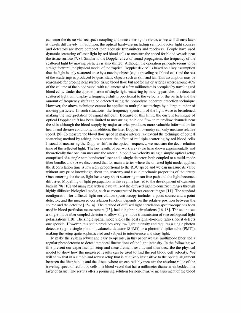
The magnitude of electrical field correlation 𝑔1 under different flow speeds of blood is shownin semi-log plots in Figure 2-4(a), where each figure shows measurements performed with adifferent tube diameter. The x-axis of each plot is the logarithmic of 𝜏 in the correlation function.From these plots we made two interesting observations: (a) At relatively low blood flow speed,the curve shows a characteristic analogous to the “Fermi-Dirac distribution function” if wetreat ln(𝜏) as “energy”; (b) at high blood speed, the curve behaves like a superposition of twoFermi-Dirac distribution functions, one at lower “energy” and another at higher “energy”. These

characteristics become more apparent if we take the derivative of 𝑔1 with ln(𝜏), showing that the“Fermi level”, ln(𝑇𝐹 ), occurs at the inflection point where the magnitude of slope reaches themaximum.

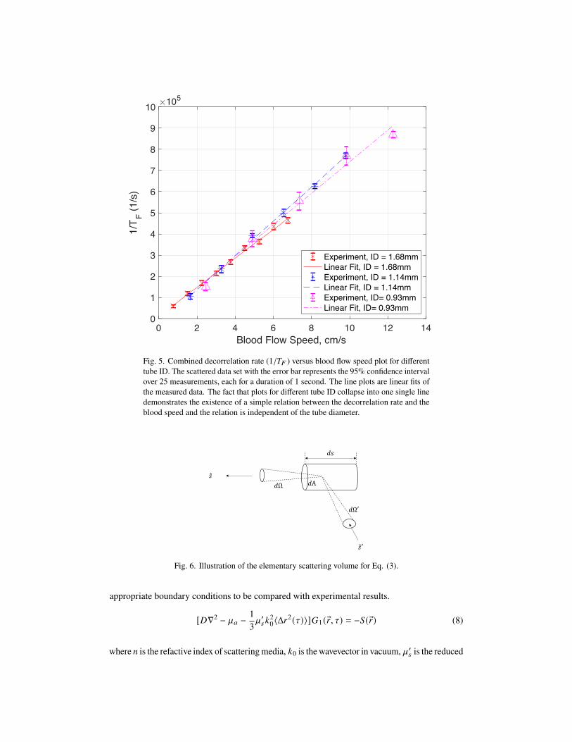
We will discuss the physics of such characteristics in the later section. By examining theinteresting features of the measured electrical field correlation 𝑔1, we can extract the “Fermienergy, 𝜖𝐹” or ln(𝑇𝐹 ). In the low blood speed regime where the|𝑔1 | plot shows two superimposedFermi-like functions, we chose the inflection point of the lower energy function (i.e. in the regimeof smaller ln(𝜏) values). We will elucidate the reasons for such a choice in the next section.Essentially each of the two superimposed Fermi-like functions represents a corresponding regimeof light scattering mechanisms. Figures 2-4(b) show the plot of 1/𝑇𝐹 (which is equivalent to𝑒−𝜖𝐹 ) versus the blood flow velocity with different tube diameters. Amazingly, we obtain asimple linear relation between 1/𝑇𝐹 and the blood speed. More interestingly, we have foundthat the 1/𝑇𝐹 versus speed curve is independent of the tube diameter. As shown in Fig. 5, thethree curves of 1/𝑇𝐹versus speed measured from different tube diameters completely overlapand can be represented by one simple relation independent of the tube diameter. This resultsuggests that our measurement setup can potentially measure the blood speed in different arterysizes without having to know the exact dimension of the blood vessel diameter. This discovery isvery important in practical applications because it shows that from the 𝑔1 (𝜏) curve, which can beobtained from the correlation of the photocurrent, we can obtain the speed of the blood directlyfor different arteries at a given position without any prior knowledge of the anatomy of the bloodvessel. The discovery of this important relation requires a sound physical foundation, to rule outthe possibility for being simply coincidental. The physical model and mathematical analysis willbe discussed next.

3. Physical Models

3.1. Diffused Light Equation for Moving Scatters:

In order to understand the underlining physics of the relation between the inverse of characteristicdecorrelation time, 1/𝑇𝐹 , and the flow speed of the blood, we describe the physical modeland mathematical formulation for our experiment in this section. We will outline the keysteps and, through approximations, produce an analytical relation between the blood speedand the decorrelation time. The detailed numerical results for more general analyses withoutapproximations will be presented in a separate paper.

People usually take two approaches to model light propagation in a strongly scattered biologicalmedium. In one approach, we start with the wave equation and introduce the scatteringand absorption characteristics along the optical path. Despite its rigor in the mathematicalformulation, to make the result useful, approximations have to be made to make the problemsolvable. Twersky’s theory and Dyson’s equation fall into this category [10]. In another approach,we can formulate the problem in a transport equation that deals with photon energy transport.These two methods eventually give rise to the same result. In this paper we take the secondapproach because of its relative simplicity.

The governing equation is a radiative transfer equation (RTE) in the following form:

𝑑𝐼 (®𝑟, 𝑠)𝑑𝑠

= −𝜌 𝜎𝑡 𝐼 (®𝑟, 𝑠) + 𝜌𝜎𝑠

∫4𝜋

𝑝(𝑠, 𝑠′)𝐼 (®𝑟, 𝑠′) 𝑑Ω′ + 𝑆(®𝑟, 𝑠) (3)

in which 𝐼 is the light specific intensity with a unit 𝑊𝑚−2𝑠𝑟−1 ,𝜌 is the particle concentration,𝜎𝑠 is the scattering cross section, 𝜎𝑡 is the total scattering cross section which is the summationof scattering cross section and absorption cross section. 𝑝(𝑠, 𝑠′) is the normalized differentialscattering cross section which is sometimes called the phase function and it’s unitless, and 𝑆(®𝑟, 𝑠)is the source intensity which has a unit of 𝑊𝑚−3𝑠𝑟−1. Figure 6 illustrates the orientations and

10-6 10-5 10-4 10-3

Correlation Time, (s)

0.4

0.6

0.8

1

g 1

(a)0.8 cm/s1.5 cm/s2.3 cm/s2.3 cm/s3.8 cm/s4.5 cm/s5.3 cm/s6.0 cm/s6.8 cm/s

0 1 2 3 4 5 6 7Blood Flow Speed, cm/s

0

2

4

1/T F (1

/s)

105 (b)

ExperimentLinear Fit

Fig. 2. (a) Measured E-field correlation function (𝑔1) versus flow speed of whole bloodfor a tube diameter of 1.68mm. (b) By taking the inverse of the correlation time atthe first inflection point in (a), the decorrelation rate (1/𝑇𝐹 ) is plotted versus the flowspeed. The scattered data set with error bars represents the 95% confidence intervalover 25 measurements, each for a duration of 1 second. The dashed line is a linear fit ofthe measured data.

coordinates for an infinitesimal scattering volume. Eq. (3) contains 5 coordinates: 𝑥, 𝑦, 𝑧, \, 𝜙where 𝑥, 𝑦, 𝑧 define the position vector ®𝑟 of the light intensity, and \, 𝜙 represent the beam’spropagation direction. The unit vectors 𝑠′ and 𝑠 represent the direction of the incident light andthe propagation direction after scattering.

Solving Eq. (3) would produce the full solution for the light scattering problem for any scatterconcentration. However, Eq. (3) is very complicated to solve. Fortunately, in most biologicalsamples, the scatter density is so high that photons quickly lose the memory of their path historiesafter multiple scatterings and it can be justified to assume the light intensity depends on itsposition (𝑥, 𝑦, 𝑧) with a slight flux flow in the direction of propagation (\, 𝜙). This would lead toa simplification of the problem, and the average intensity could be described by the diffusionequation which is only dependent on the position (𝑥, 𝑦, 𝑧). Mathematically, it means that we canexpand the light intensity in spherical harmonics by keeping the zero order and first order term.

𝐼 (®𝑟, 𝑠) ' 14𝜋

𝑈 (®𝑟) + 34𝜋

®𝐹 (®𝑟) · 𝑠 (4)

where the first term is the average intensity and the second term is the small photon flux in thedirection of propagation. Applying the diffusion approximation to the RTE, we can obtain asteady state diffusion Eq. (5) to model light propagation in a diffusive medium when the scattersare not moving. As light needs to be scattered multiple times to become diffusive, an important

10-6 10-5 10-4 10-3


0.4

0.6

0.8

1

g 1

(a)4.5 cm/s5.3 cm/s6 cm/s6.8 cm/s8.2 cm/s9.8 cm/s

2 4 6 8 10Blood Flow Speed, cm/s

0

2

4

6

8

1/T F (1

/s)

105 (b)



requirement for the diffusion approximation is that the cross section for light scattering is muchstronger than the cross section for light absorption. A problem would arise when dealing withlight intensity close to the boundary since the light is highly directional at the boundary, violatingthe diffusive condition. Different boundary conditions have been explored to resolve this problem,including adoption of an extended boundary condition which uses Taylor expansion to convertthe Robin boundary condition into a Dirichlet type boundary condition to simplify the solutionfor Eq. (5) [25].

[𝐷∇2 − `𝑎]𝑈 (®𝑟) = −𝑆(®𝑟) (5)

where 𝐷 = 1/3`′𝑠 is the photon diffusivity with a unit of meter and `′

𝑠 is the reduced scatteringcoefficient. `𝑎 is the absorption coefficient with a unit 𝑚−1. 𝑆(®𝑟) is the source (unit of 𝑊𝑚−3)that depends only on the location but not on the propagation direction, different from 𝑆(®𝑟, 𝑠)in Eq. (3).When the scatters exhibit motions, the scattered intensity would include time as aparameter. For statistical optics, it is natural to use field correlation function to capture thisdynamic process. Here, we are still talking about the steady state response of the system so thatthe time dependence can be represented as a parameter in the differential equation.

We start with the case of single scattering event by a moving object. The normalized single

10-6 10-5 10-4 10-3


0.4

0.6

0.8

1

g 1

(a)2.5 cm/s4.9 cm/s7.4 cm/s9.8 cm/s12.3 cm/s

2 4 6 8 10 12Blood Flow Speed, cm/s

0

5

10

1/T F (1

/s)

105 (b)



scattering function can be written as:

𝑔𝑠1 (𝜏) =〈𝐸 (𝑡)𝐸∗ (𝑡 + 𝜏)〉〈𝐸 (𝑡)𝐸∗ (𝑡)〉 = exp

(− 1

6𝑞2〈Δ𝑟2

𝑖 (𝜏)〉)

(6)

where 𝑔𝑠1 is the single scattering normalized correlation function, 𝐸 is the scalar electrical field oflight, 𝑞 is the photon momentum transfer by each scattering, 〈Δ𝑟2

𝑖(𝜏)〉 is the RMS displacement

of the scatters in a duration of 𝜏. The above equation describes the electrical field correlationfunction due to single scattering. This single scattering function can be incorporated into theradiative transfer equation, yielding the so-called correlation transfer equation which is thedynamic counter part of the static radiative transfer equation [26]:

𝑑𝐺1 (®𝑟, 𝑠, 𝜏)𝑑𝑠

= −𝜌𝜎𝑡𝐺1 (®𝑟, 𝑠, 𝜏) + 𝜌𝜎𝑠

∫4𝜋

𝑝(𝑠, 𝑠′) 𝑔𝑠1 (𝑠, 𝑠′, 𝜏)𝐺1 (®𝑟, 𝑠, 𝜏) 𝑑Ω′ + 𝑆(®𝑟, 𝑠) (7)

Similarly, the diffusion approximation can also be applied to obtain the correlation diffusionequation which is again the counterpart of the static diffusion equation described previously.Eq. (8) is the correlation diffusion equation. The diffusion equation can then be solved with


0

1

2

3

4

5

6

7

8

9

10

1/T F (1

/s)

105

Experiment, ID = 1.68mmLinear Fit, ID = 1.68mmExperiment, ID = 1.14mmLinear Fit, ID = 1.14mmExperiment, ID= 0.93mmLinear Fit, ID= 0.93mm

Fig. 5. Combined decorrelation rate (1/𝑇𝐹 ) versus blood flow speed plot for differenttube ID. The scattered data set with the error bar represents the 95% confidence intervalover 25 measurements, each for a duration of 1 second. The line plots are linear fits ofthe measured data. The fact that plots for different tube ID collapse into one single linedemonstrates the existence of a simple relation between the decorrelation rate and theblood speed and the relation is independent of the tube diameter.

!"

"̂

"̂′

!Ω

!Ω′

!A

Fig. 6. Illustration of the elementary scattering volume for Eq. (3).

appropriate boundary conditions to be compared with experimental results.

[𝐷∇2 − `𝑎 −13`′𝑠𝑘

20〈Δ𝑟

2 (𝜏)〉]𝐺1 (®𝑟, 𝜏) = −𝑆(®𝑟) (8)

where 𝑛 is the refactive index of scattering media, 𝑘0 is the wavevector in vacuum, `′𝑠 is the reduced

scattering coefficient which is the scattering coefficient modified due to scattering anisotropy. Forisotropic scattering, the scattering coefficient would be the same reduced scattering coefficient.

3.2. Analytic Relation Between Decorrelation Time and RBC Flow Speed

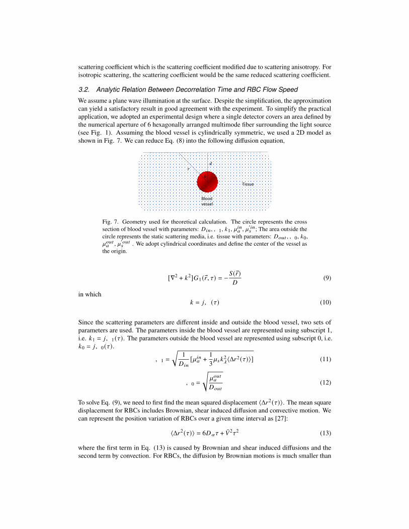
We assume a plane wave illumination at the surface. Despite the simplification, the approximationcan yield a satisfactory result in good agreement with the experiment. To simplify the practicalapplication, we adopted an experimental design where a single detector covers an area defined bythe numerical aperture of 6 hexagonally arranged multimode fiber surrounding the light source(see Fig. 1). Assuming the blood vessel is cylindrically symmetric, we used a 2D model asshown in Fig. 7. We can reduce Eq. (8) into the following diffusion equation,

Tissue

!"

#

Blood vessel

Fig. 7. Geometry used for theoretical calculation. The circle represents the crosssection of blood vessel with parameters: 𝐷𝑖𝑛, 𝑊1, 𝑘1, `𝑖𝑛𝑎 , `′𝑖𝑛

𝑠 ; The area outside thecircle represents the static scattering media, i.e. tissue with parameters: 𝐷𝑜𝑢𝑡 , 𝑊0, 𝑘0,`𝑜𝑢𝑡𝑎 , `′𝑜𝑢𝑡

𝑠 . We adopt cylindrical coordinates and define the center of the vessel asthe origin.

[∇2 + 𝑘2]𝐺1 (®𝑟, 𝜏) = −𝑆(®𝑟)𝐷

(9)

in which𝑘 = 𝑗𝑊 (𝜏) (10)

Since the scattering parameters are different inside and outside the blood vessel, two sets ofparameters are used. The parameters inside the blood vessel are represented using subscript 1,i.e. 𝑘1 = 𝑗𝑊1 (𝜏). The parameters outside the blood vessel are represented using subscript 0, i.e.𝑘0 = 𝑗𝑊0 (𝜏).

𝑊1 =

√︂1𝐷𝑖𝑛

[`𝑖𝑛𝑎 + 13`𝑠𝑘

2_〈Δ𝑟2 (𝜏)〉] (11)

𝑊0 =

√︄`𝑜𝑢𝑡𝑎

𝐷𝑜𝑢𝑡

(12)

To solve Eq. (9), we need to first find the mean squared displacement 〈Δ𝑟2 (𝜏)〉. The mean squaredisplacement for RBCs includes Brownian, shear induced diffusion and convective motion. Wecan represent the position variation of RBCs over a given time interval as [27]:

〈Δ𝑟2 (𝜏)〉 = 6𝐷𝛼𝜏 + �̄�2𝜏2 (13)

where the first term in Eq. (13) is caused by Brownian and shear induced diffusions and thesecond term by convection. For RBCs, the diffusion by Brownian motions is much smaller than

the shear induced diffusion [28]. The flow of RBCs inside arteries can be modeled by a laminarflow and the diffusion coefficient can be represented as [29]

𝐷𝛼 = 𝛼𝑠

��𝜕𝑣𝑅𝐵𝐶

𝜕𝑟

�� = 43𝛼𝑠

𝑉𝑚𝑎𝑥

𝑎(14)

𝛼𝑠 is a parameter describing the interaction strength among blood cells due to shear and itsvalue has been measured experimentally [30–36].The radial dependent shear rate is usuallyreplaced by its average value due to the fact that multiple scattering will lead to an ensembleaveraging across all radial locations . For tissue blood perfusion, the slow flow speed and smallblood vessel diameter make the diffusive motion the dominant effect compared to the convectivemotion [37]. The situation is reversed, however, for main arteries and our phantom model wherethe vessel inner diameter is of millimeter size and the blood flow speed is several centimetersper second [38]. In such cases, the convective motion becomes the dominant effect. Hence inour analysis, we have ignored the diffusion contribution and included only the convective flowcontribution in Eq. (13).

We can then write the general solution of the correlation function in Eq. (9) as follows,

𝐺1 (®𝑟, 𝜏) = 𝐺𝑖𝑛1 (®𝑟, 𝜏) + 𝐺𝑠𝑐

1 (®𝑟, 𝜏) (15)

The first term is the inhomogeneous solution and the second term is the homogeneous solutionfor Eq. (9) in the absence of the source. The diffusion equation under a given boundarycondition can be solved in polar coordinates and the method of separation of variables. For anapproximate analytic solution, we kept only the zeroth order term since all higher order terms areinsignificant compared with the zeroth order term. A continuity boundary condition is appliedat the cylinder interface between the blood vessel and the surrounding tissue. The air-tissuesurface is ignored for simplicity in the solution. After solving the differential equation withsome approximations based on the numerical value of actual tissue and blood cell scatteringproperties, the normalized correlation function 𝑔1 can be written in the form of Eq. (16), inspiredfrom the Fermi-Dirac function in semiconductor physics (i.e. by performing the transformations:ln(𝜏) = 𝜖, ln(𝑇𝐹 ) = 𝐸𝐹 ,Eq. (16) is similar to the Fermi-Dirac function).

𝑔1 (𝑟, 𝑎, \, 𝜏) =1 − 𝑔1 (𝑟, 𝑎, \,∞)

1 + 𝜏𝑇𝐹

+ 𝑔1 (𝑟, 𝑎, \,∞) (16)

1𝑇𝐹

≈ 𝑉𝑛𝑘0

√︄`′𝑖𝑛𝑠

3`𝑖𝑛𝑎(17)

where V is the flow velocity of blood, n is the refractive index of blood, 𝑘0 is the wavevector of784 𝑛𝑚 light in vacuum, `′𝑖𝑛

𝑠 is the reduced scattering coefficient of blood (𝑚−1), and `𝑖𝑛𝑎 is theabsorption coefficient of blood (𝑚−1). If we define 𝑇𝐹 as the characteristic decorrelation time,and 1/𝑇𝐹 as the characteristic decorrelation rate, we obtain the key relation that the characteristicdecorrelation rate is only a function of flow speed and blood optical parameters, as shown in Eq.(17). In Eq. (16), 𝑔1 (𝑟, 𝑎, \,∞) is the asymptotic value of 𝑔1 when 𝜏 approaches infinity, and itsvalue is a function of detector position and blood vessel diameter. In a separate study that solvesEq. (9) numerically, we have validated the approximations that led to the analytic solution for 𝑔1in Eq. (16) and most importantly, the linear relation between 1/𝑇𝐹 and the blood flow velocity.We have also shown that the decorrelation time for 2D and 3D analyses is nearly the same. Thedetailed mathematical derivations as well as the numerical computations for the diffused lightmodel will be described in a separate publication.

From the approximated relation in Eq. (17), we find that the characteristic decorrelation rateis proportional to the flow speed. The proportional constant has a square root dependence onthe ratio between the scattering coefficient and the absorption coefficient. This is intuitive sincescattering events cause dephasing, and light absorption would terminate the scattering process.

4. Discussions

The measured characteristic decorrelation rate (1/𝑇𝐹 ) is obtained by calculating the first inflectionpoint of the curves in Figure 2-4. The behavior of the curves at longer time is more complicated,and can be explained by other slower decorrelation processes than convection such as shearinduced diffusion, thus yielding two superimposed Fermi-like functions as shown in Figure 2-4.To use the model described in the previous section, we need to focus on the short time behaviordriven by convection. Figure 8 shows the calculated and measured characteristic decorrelationrate under different flow speeds and tube diameters. An excellent agreement between theory andexperiment was achieved, confirming that in the regime where convective flow is the dominatingfactor for decorrelation, the characteristic decorrelation rate is proportional to the blood speedand independent of the vessel diameter.


0

1

2

3

4

5

6

7

8

9

10

1/T F (1

/s)

105

Experiment, ID = 1.68mmExperiment, ID = 1.14mmExperiment, ID= 0.93mmTheory

Fig. 8. Comparison between theoretical calculations (from Eq. 17) and experimentallymeasured decorrelation rates under different blood flow speeds and tube diameters.The scattered data set with the error bar represents the 95% confidence interval over 25measurements. Each measurement took 1 second. The following parameters are usedin the calculations: 𝑛 = 1.36, `′𝑖𝑛

𝑠 = 1600𝑚−1and `𝑖𝑛𝑎 = 1000𝑚−1 for deoxygenatedblood [39–42].

5. Conclusion

In this work, we demonstrated a simple technique to directly measure the blood flow speed inmain arteries based on the diffused light model. The device uses a single fiber bundle, a diode

laser, and a photoreceiver. The concept is demonstrated with a phantom that uses intralipidhydrogel to model the biological tissue and an embedded glass tube with flowing human bloodto model the blood vessel. The correlation function of the measured photocurrent was used tofind the electrical field correlation function via the Siegert Relation. Interestingly the measuredelectric field correlation function 𝑔1 (𝜏) and ln(𝑇𝐹 ) shows a relation similar to the Fermi-Diracfunction, allowing us to define the 𝑙𝑛(𝜏), equivalent to the “Fermi energy” occurring at the firstinflection point of 𝑔1 (𝜏). Surprisingly, the value 1/𝑇𝐹 , which we call characteristic decorrelationrate, is found to be linearly proportional to the blood speed and is independent of the diameter ofthe tube diameter over the size and speed ranges for major arteries. This striking property canbe explained by an approximate analytic solution for the diffused light equation in the regimewhere the convective flow would dominate the decorrelation. This discovery is highly significantbecause, for the first time, we can use a simple device to directly measure the blood speed inmajor arteries without any prior knowledge or assumption about the geometry or mechanicalproperties of the blood vessels. A non-invasive method of measuring arterial blood speedproduces important information about health conditions. Although the device and setup canbe further optimized (e.g. adding different light wavelengths) and the physical model can beexpanded to acquire more information from the measurements, the work has paved its way to anew promising modality for measurements of blood supplies to vital organs.

References1. C. Wang, X. Li, H. Hu, L. Zhang, Z. Huang, M. Lin, Z. Zhang, Z. Yin, B. Huang, H. Gong et al., “Monitoring of the

central blood pressure waveform via a conformal ultrasonic device,” Nat. biomedical engineering 2, 687 (2018).2. K. Stewart, S. Dangelmaier, P. Pott, and J. Anders, “Investigation of a non-invasive venous blood flow measurement

device: Using thermal mass measurement principles,” Curr. Dir. Biomed. Eng. 5, 179–182 (2019).3. A. Jayanthy, N. Sujatha, and M. R. Reddy, “Measuring blood flow: techniques and applications–a review,” Int. J. Res.

Rev. Appl. Sci 6, 203–216 (2011).4. C. Poelma, A. Kloosterman, B. P. Hierck, and J. Westerweel, “Accurate blood flow measurements: are artificial

tracers necessary?” PloS one 7 (2012).5. H. L. Blumgart and O. C. Yens, “Studies on the velocity of blood flow: I. the method utilized,” The J. clinical

investigation 4, 1–13 (1927).6. S. J. Pietrangelo, H.-S. Lee, and C. G. Sodini, “A wearable transcranial doppler ultrasound phased array system,” inIntracranial Pressure & Neuromonitoring XVI, (Springer, 2018), pp. 111–114.

7. S. Kashima, M. Nishihara, T. Kondo, and T. Ohsawa, “Model for measurement of tissue oxygenated blood volume bythe dynamic light scattering method,” Jpn. journal applied physics 31, 4097 (1992).

8. S. Kashima, A. Sohda, H. Takeuchi, and T. Ohsawa, “Study of measuring the velocity of erythrocytes in tissue by thedynamic light scattering method,” Jpn. journal applied physics 32, 2177 (1993).

9. V. Rajan, B. Varghese, T. G. van Leeuwen, and W. Steenbergen, “Review of methodological developments in laserdoppler flowmetry,” Lasers medical science 24, 269–283 (2009).

10. A. Ishimaru, Wave propagation and scattering in random media, vol. 2 (Academic press New York, 1978).11. L. V. Wang and H.-i. Wu, Biomedical optics: principles and imaging (John Wiley & Sons, 2012).12. T. Durduran, R. Choe, W. B. Baker, and A. G. Yodh, “Diffuse optics for tissue monitoring and tomography,” Reports

on Prog. Phys. 73, 076701 (2010).13. K. Vishwanath and S. Zanfardino, “Diffuse correlation spectroscopy at short source-detector separations: Simulations,

experiments and theoretical modeling,” Appl. Sci. 9, 3047 (2019).14. S. Zanfardino and K. Vishwanath, “Sensitivity of diffuse correlation spectroscopy to flow rates: a study with tissue

simulating optical phantoms,” in Medical Imaging 2018: Physics of Medical Imaging, vol. 10573 (InternationalSociety for Optics and Photonics, 2018), p. 105732K.

15. D. A. Boas, S. Sakadžić, J. J. Selb, P. Farzam, M. A. Franceschini, and S. A. Carp, “Establishing the diffuse correlationspectroscopy signal relationship with blood flow,” Neurophotonics 3, 031412 (2016).

16. T. Durduran and A. G. Yodh, “Diffuse correlation spectroscopy for non-invasive, micro-vascular cerebral blood flowmeasurement,” Neuroimage 85, 51–63 (2014).

17. A. Torricelli, D. Contini, A. Dalla Mora, A. Pifferi, R. Re, L. Zucchelli, M. Caffini, A. Farina, and L. Spinelli,“Neurophotonics: non-invasive optical techniques for monitoring brain functions,” Funct. neurology 29, 223 (2014).

18. K. Verdecchia, M. Diop, L. B. Morrison, T.-Y. Lee, and K. S. Lawrence, “Assessment of the best flow modelto characterize diffuse correlation spectroscopy data acquired directly on the brain,” Biomed. optics express 6,4288–4301 (2015).

19. J. Rička, “Dynamic light scattering with single-mode and multimode receivers,” Appl. optics 32, 2860–2875 (1993).

20. P. Lai, X. Xu, and L. V. Wang, “Dependence of optical scattering from intralipid in gelatin-gel based tissue-mimickingphantoms on mixing temperature and time,” J. biomedical optics 19, 035002 (2014).

21. B. W. Pogue and M. S. Patterson, “Review of tissue simulating phantoms for optical spectroscopy, imaging anddosimetry,” J. biomedical optics 11, 041102 (2006).

22. S. T. Flock, S. L. Jacques, B. C. Wilson, W. M. Star, and M. J. van Gemert, “Optical properties of intralipid: aphantom medium for light propagation studies,” Lasers surgery medicine 12, 510–519 (1992).

23. H. Ding, J. Q. Lu, K. M. Jacobs, and X.-H. Hu, “Determination of refractive indices of porcine skin tissues andintralipid at eight wavelengths between 325 and 1557 nm,” JOSA A 22, 1151–1157 (2005).

24. H. Z. Cummins and H. L. Swinney, “Iii light beating spectroscopy,” in Progress in optics, vol. 8 (Elsevier, 1970), pp.133–200.

25. R. C. Haskell, L. O. Svaasand, T.-T. Tsay, T.-C. Feng, M. S. McAdams, and B. J. Tromberg, “Boundary conditions forthe diffusion equation in radiative transfer,” JOSA A 11, 2727–2741 (1994).

26. D. A. Boas and A. G. Yodh, “Spatially varying dynamical properties of turbid media probed with diffusing temporallight correlation,” JOSA A 14, 192–215 (1997).

27. M. Belau, W. Scheffer, and G. Maret, “Pulse wave analysis with diffusing-wave spectroscopy,” Biomed. optics express8, 3493–3500 (2017).

28. X. Wu, D. Pine, P. Chaikin, J. Huang, and D. Weitz, “Diffusing-wave spectroscopy in a shear flow,” JOSA B 7, 15–20(1990).

29. C. A. Owen and M. Roberts, “Arterial vascular hemodynamics,” J. Diagn. Med. Sonogr. 23, 129–140 (2007).30. H. Goldsmith and J. Marlow, “Flow behavior of erythrocytes. ii. particle motions in concentrated suspensions of

ghost cells,” J. Colloid Interface Sci. 71, 383–407 (1979).31. C. Funck, F. B. Laun, and A. Wetscherek, “Characterization of the diffusion coefficient of blood,” Magn. resonance

medicine 79, 2752–2758 (2018).32. E. E. Nanne, C. P. Aucoin, and E. F. Leonard, “Shear rate and hematocrit effects on the apparent diffusivity of urea in

suspensions of bovine erythrocytes,” ASAIO journal (American Soc. for Artif. Intern. Organs: 1992) 56, 151 (2010).33. J. M. Higgins, D. T. Eddington, S. N. Bhatia, and L. Mahadevan, “Statistical dynamics of flowing red blood cells by

morphological image processing,” PLoS computational biology 5 (2009).34. J. Biasetti, P. G. Spazzini, U. Hedin, and T. C. Gasser, “Synergy between shear-induced migration and secondary flows

on red blood cells transport in arteries: considerations on oxygen transport,” J. Royal Soc. Interface 11, 20140403(2014).

35. W. Cha and R. L. Beissinger, “Evaluation of shear-induced particle diffusivity in red cell ghosts suspensions,” KoreanJ. Chem. Eng. 18, 479–485 (2001).

36. J. Tang, S. E. Erdener, B. Li, B. Fu, S. Sakadzic, S. A. Carp, J. Lee, and D. A. Boas, “Shear-induced diffusion of redblood cells measured with dynamic light scattering-optical coherence tomography,” J. biophotonics 11, e201700070(2018).

37. S. Sakadžić, D. A. Boas, and S. A. Carp, “Theoretical model of blood flow measurement by diffuse correlationspectroscopy,” J. biomedical optics 22, 027006 (2017).

38. I. T. Gabe, J. H. GAULT, J. ROSS JR, D. T. MASON, C. J. MILLS, J. P. SCHILLINGFORD, and E. Braunwald,“Measurement of instantaneous blood flow velocity and pressure in conscious man with a catheter-tip velocity probe,”Circulation 40, 603–614 (1969).

39. E. N. Lazareva and V. V. Tuchin, “Blood refractive index modelling in the visible and near infrared spectral regions,”J. Biomed. Photonics & Eng. 4 (2018).

40. H. Li, L. Lin, and S. Xie, “Refractive index of human whole blood with different types in the visible and near-infraredranges,” in Laser-Tissue Interaction XI: Photochemical, Photothermal, and Photomechanical, vol. 3914 (InternationalSociety for Optics and Photonics, 2000), pp. 517–521.

41. N. Bosschaart, G. J. Edelman, M. C. Aalders, T. G. van Leeuwen, and D. J. Faber, “A literature review and noveltheoretical approach on the optical properties of whole blood,” Lasers medical science 29, 453–479 (2014).

42. S. L. Jacques, “Optical properties of biological tissues: a review,” Phys. Medicine & Biol. 58, R37 (2013).

Documents

ALEX CE ZHANG 1 YU-HWA LO1*