Working Paper 09-68 Departamento de Economía de la Empresa Business Economics Series 08 Universidad Carlos III de Madrid October, 2009 Calle Madrid, 126 28903 Getafe (Spain) Fax (34-91) 6249607

OPTIMAL RISK IN MARKETING RESOURCE ALLOCATION∗

Alejandro Balbás1, Mercedes Esteban-Bravo2 and José M. Vidal-Sanz 3

Abstract Marketing resource allocation is increasingly based on the optimization of expected returns on investment. If the investment is implemented in a large number of repetitive and relatively independent simple decisions, it is an acceptable method, but risk must be considered otherwise. The Markowitz classical mean-deviation approach to value marketing activities is of limited use when the probability distributions of the returns are asymmetric (a common case in marketing). In this paper we consider a unifying treatment for optimal marketing resource allocation and valuation of marketing investments in risky markets where returns can be asymmetric, using coherent risk measures recently developed in finance. We propose a set of first order conditions for the solution, and present a numerical algorithm for the computation of the optimal plan. We use this approach to design optimal advertisement investments in sales response management. Keywords: Resource allocation, coherent risk measures, optimization, sales response models.

∗ This research has been partly supported by the Ministerio de Educación y Ciencia of Spain, through the projects SEJ2007-65897/ECON and SEJ2006-15401-C04, and Comunidad Autónoma de Madrid, through the project S-0505/TIC/000230. 1 Alejandro Balbas, Department of Business Administration, University Carlos III de Madrid, C/ Madrid 126, 28903 Getafe (Madrid), Spain; e-mail: balbas@emp.uc3m.es 2 Mercedes Esteban-Bravo, Department of Business Administration, University Carlos III de Madrid, C/ Madrid 126, 28903 Getafe (Madrid), Spain; e-mail: mesteban@emp.uc3m.es 3 Jose M. Vidal-Sanz, Department of Business Administration, University Carlos III de Madrid, C/ Madrid 126, 28903 Getafe (Madrid), Spain; e-mail: jvidal@emp.uc3m.es

1 Introduction

Firms spend billions of dollars on management strategic and tactic investments,ranging from new product development, to logistics and supply chain decisions,sales force scheduling, market research, communication, sales promotion, andother marketing expenditures. In uncertain markets firm stakeholders increas-ingly want proof of their marketing investment payback. Traditionally, manycompanies allocate resources using widespread rules-of-thumb. For example,funding advertising or sales-forces with a “percentage-of-sales”, or a “bottom-up” rule investing until some output-measurement level is achieved, or justimitating the decisions taken by strong competitors or industry-benchmarks.The caveat with these practices is that they are not based on controlled studies.Just because the company is doing well, does not mean that the investment iscause for it, and even so, it does not mean that the same strategy will work inthe future or for a different company.The economic value of any investment is the return on investment (ROI); i.e.,

the net present value or sum of discounted future returns minus the discountedvalue of the expenditure (including all variable costs and the amortization ofthe proportional part of any fixed costs). If this value is computed at customerlevel, it is known as the Customer Lifetime Value (CLV) for the firm. Thereturn on investment, at firm/specific customers level, should be maximized todetermine the resource allocation, and the optimal value must be positive orthe investment should not be undertaken. Under perfect certainty, a marketingaction will have only one possible return and marketing decisions can be easilyplanned. However the assumption of perfect foresight is unrealistic and can givemisleading insights — the actual ROI and CLV fluctuates randomly.In an uncertain context, the optimal marketing plan involves choosing be-

tween alternative projects assessing their random values. The marketing lit-erature essentially focuses on expected returns maximization. Following theseminal works by Little (1970, 1975), the developments in statistics & econo-metric theory, OR, and computational capacity for storing and processing data,have spurred the development of management science decision methods for re-source allocation (see e.g., Little and Lodish 1969, Lodish 1971, Little 1975,Blattberg and Hoch 1990, Wierenga et al. 1999, Wierenga 2008, Eisenstein andLodish 2002, Divakar et al. 2005, Natter et al. 2007, Tirenni et al. 2007).The management science procedures essentially consist of two stages. In stageone, the available information (e.g., market data, experiments, and manager-ial expertise) is used to estimate the firm expected return conditionally on theinvestment decision and other exogenous variables, and in the second one theoptimal decision is made by maximizing the expected economic outcome. Ifthe model includes exogenous variables, then what-if optimal decisions can beconsidered for different scenarios. Nowadays, these tasks are increasingly im-plemented by firms using computerized platforms known as Decision SupportSystems (DSS) integrating statistical data and managerial judgment to estimatedemands and then to apply optimization tools, see e.g. Divakar et al. (2005).For a literature review see Little, (2004a, 2004b), Gupta and Steenburgh (2008),

1

Shankar (2008) and Wierenga (2008).Expected value is the most basic form of risk analysis. If the investment is

implemented in a large number of repetitive and relatively independent simpledecisions, it is an acceptable method. But for distinctive decisions it is not soconvenient, since maximizing expected value of investments managers do nottake into account the returns’ fluctuations and can, therefore, expose compa-nies to considerable risks. Good investment is not just a matter of “pocketingmoney” on a short-term horizon, and we observe that after some time a pro-portion of companies fail with little control about the dimension of failure. Therecent world-wide financial crisis shows how badly an investor may be positionedwithout notice due to the emphasis on average returns. In an uncertain market,risk adverse executives must optimize the expected payback on their investmentswhilst penalize the intrinsic risks. Additionally, if the model includes exogenousvariables, then the optimal resource allocation should anticipate the impact onthe plan of exogenous scenario changes.The idea is to invest in projects that have the minimum level of risk with

the highest possible return. However, most of the customer relationships andmarketing valuation literature use the expected ROI and the balance betweenreturn and risk is not considered. As Hogan et al. (2002) point out, an un-resolved challenge for marketers is how to adjust for the differential of risk ofdifferent customers. Even if risk is taken into account, the decision is based onthe variance (see, e.g., Holthausen and Assmus 1982, Zhou and Pham, 2004,and Prakhya, Rajiv and Srinivasan, 2006), giving misleading results when thereturns have asymmetric probability distributions.In the financial context, Markowitz (1952) lays the basis for valuing a portfo-

lio of investments in terms of expected returns and standard-deviations. How-ever, financial and marketing investments usually have asymmetric probabil-ity distributions. In this case, the variance is not an accurate measure of theinvestor risk preferences if a downside risk is more weighted than an upsiderisk. Markowitz (1991) acknowledges this shortcoming. Since returns are usu-ally asymmetric, the use of mean-variance methods often provide misleadingresults. This fact is nowadays widespread in finance theory, where a set of alter-native valuation methods such as Value at Risk, and Conditional Value at Riskare usually considered. This leads to the notions of coherent risk and deviationmeasures developed by Artzner et al. (1997, 1999) and Rockafellar et al. (2006).In this paper we present a procedure for marketing resource allocation, ac-

counting for associated risk. In particular we consider coherent risk measures,and present a numerical procedure for the computation of this problem in re-source allocation.The rest of the paper is structured as follows. In Section 2 we review the

literature about optimal planning under uncertainty and coherent risk measures.Section 3 presents the general method for resource allocation. In Section 4, wepresent an application to illustrate the behavior of the method for sales responsemanagement. In the concluding remarks section we summarize the findings.

2

2 Optimal resource investment strategies

In this section we consider the problem of optimal investment in a managementcontext, using coherent risk measures. Consider a probabilistic space (Ω,A, P ),where ω belongs to a set Ω representing states of nature with probability P . Thespace of feasible investment decisions is X ⊂ Rn. Often X is a compact set, forexample a budget set. We assume that the uncertain return outcome associatedto each decision x ∈ X is a random variable Yx = Y (x, ω) with finite variance,and denote by Y = Yx : x ∈ X. Each random variable Yx ∈ Y induces a Borelprobability measure πx = P Y −1x on R, describing the uncertainty associatedto the decision x. We will denote the cumulative distribution by FYx (y) =πx (−∞, y] . Usually, some preliminary statistical analysis allows the decisionmaker to study the distribution πx. This setup can be applied to the majority ofthe management decision problems, where company returns to decisions x ∈ Xis given by the random variables Yx.The central investment decision making problem consists of choosing x ∈ X

so as to minimize risks in Yx. Risk is an ambiguous word. It has been associatedwith statistical variances and volatility, but in the investment literature risk isgenerally considered as an overall assessment of potential losses. Henceforth, wewill use the expression “deviation measure” when considering generalizations ofstandard deviation designed to assess variability around the mean, whereas theexpression “risk measures” will be used in the assessment of losing scenarios(Yx < 0). The manager must select the investment x∗ solving

minx∈X

ρ (Yx) (1)

where ρ is a risk measure penalizing losses. Classical risk functions are theminus expected return ρM (Yx) = E [−Yx] which is insensitive to risks, and evenfor investments with E [−Yx] = 0 investors are exposed to large losses for tail-outcomes −Yx > 0. Expectations are suitable for some long-range strategieswhere stochastic ups and downs tend to safely average out, but not in a short-range operation. Markowitz’s (1952) criteria

ρMD (Yx) = E [−Yx] + γpV ar [Yx] (2)

where γ > 0 is a “safety” scaling, is a widespread method to introduce safetymargins using standard deviations. It enhances solutions x∗ with expected lossE [−Yx∗ ] not just zero but reassuringly negative. This is due to the fact thatlosses −Yx > 0 will occur only in states associated to the high end of thedistribution of −Yx lying more than γ

pV ar [Yx] units above the mean loss.

Unfortunately, the mean-deviation risk penalizes investments with high re-turns fluctuations around the mean. As the distribution πx is generally asym-metric (a distributional asymmetry is found in the returns of almost any man-agerial investment), the use of mean-variance methods often provides misleadingresults. One of the difficulties is to construct a proper measure of risk ρ (Yx)allowing a higher weight for downside risks than for upside ones.

3

Over the past decades, the important limitations of the mean-variance andexpected utility approaches have led banks and financial regulators to developa variety of alternative risk measures for the purpose of better quantifying thefinancial risks that they face. Most of these methods can be extended to themanagement and marketing context. A popular risk measure is the Value atRisk (VaR) with confidence level α ∈ (0, 1) , defined as a distributional percentileof losses,

V aRα (Yx) = −F−1Yx(α) = − inf z : P (Yx ≤ z) > α ,

which use was proposed by the Global Derivatives Study Group (GDSG, 1993).This criterion has been already used to measure risk in marketing investments,by Dickson and Giglierano (1986) who call it sinking-the-boat-risk. If Yx is nor-mally distributed, the minimization of VaR is almost equivalent to the Markowitzmean-deviation model, as V aRα (Yx) = E [−Yx] + Φ−1 (α)

pV ar [Yx], where

Φ−1 (α) is the α-quantile of a standard normal distribution. But for asymmet-ric distributions it has a better performance.A major problem of the VaR is that it does not inform about the likely

size of the loss that we can have when that value is achieved, as a consequencethe Conditional Value-at-Risk (CVaR) risk measure with confidence level α hasbeen proposed in the finance literature, given by

CV aRα (Y ) = − 1α

Z α

0

F−1Y ( ) d =1

α

Z α

0

V aR (Y ) d .

If Y has an absolutely continuous probability distribution, then

CV aRα (Y ) = −E£Y |Y ≤ F−1Y (α)

¤= −E [Y |Y ≤ −V aRα (Y )] .

and we can interpret the CV aR as the expected shortfall or expected loss for aninvestment whose return does not exceed a predetermined quantile threshold.This risk measure has been recognized and encouraged by the Basel Committeeon Banking Supervision of the Bank for International Settlement (BIS, 2006).Once again, if Y is normally distributed, the minimization of CVaR is almostequivalent to the Markowitz mean-deviation model1 .There exists an alternative approach for measuring risk, based on von Neu-

mann and Morgernstern’s (1944) expected utility theory, which stems fromBernoulli’s work (1738). Regular preferences on losses (satisfying the complete-ness, transitiveness, continuity and independence axioms) can be expressed by

ρ (Y ) = −Z

u (y) dFY (y) = −Z 1

0

u¡F−1Y (y)

¢dy,

1For normally distributed returns,

CV aRα (Y ) = −E [Yx] +φ¡Φ−1 (α)

¢α

pV ar [Yx]

where φ is the density of a standard normal distribution.

4

where u is a non-negative function of the returns. A concave function u wasconsidered to introduce risk-aversion. The expected utility theory is refuted inexperiments showing that this approach is not compatible with the decision-makers behavior (e.g., Tversky and Kahneman, 1979). Wang (2000) proposedan alternative procedure, applying weights ν (·) on FY as in

Ru (y) d (ν FY ) ,

and considering also u (y) = y, leading to a more realistic risk-measure

ρ (Y ) = −Z

y d (ν FY ) (y) = −Z 1

0

F−1Y (y) dν (y) .

This family can be found in the statistical literature as L-statistics. In risk-analysis context, the weight measure ν is usually asymmetric around some an-chor point. The VaR is a particular case with

ν (y) =

½0 y ≤ α1 y > α,

and the CVaR with

ν (y) =

½y/α−1 y ≤ α1 y > α.

A variety of measures ν can be considered alike.Fueled by these developments, all the classical financial problems are be-

ing revisited by the researchers, and the new risk measures are being infusedinto insurance and finance daily practice. But not all these risk measures areequally popular, and some seem less useful for investment decision planning. Toclarify these issues, finance scholars have developed a conceptual theory of riskmeasurement.

2.1 Coherent risk measures

To successfully incorporate the new risk measures into decision models, theymust be compatible with the axiomatic required for decision making problems.Artzner et al. (1997, 1999) first present and justify a set of risk-measure ax-ioms — the axioms of coherency — and this axiomatic has become one of themost important recent achievements in the financial risk area, and they werereformulated later by Rockafellar et al. (2006). Consider the class L2 of random

variables Y with Eh|Y |2

i<∞. Having Y ∈ L2 ensures that both the mean and

the standard deviation of Y are well defined and finite. According to Rockafellaret al. (2006),

Definition 1 A function ρ defined over L2 is said to be a coherent measure (inthe basic sense) if it satisfies:(R1) ρ (c) = −c for all c ∈ R.(R2) Convexity: ρ ((1− λ)Y + λY 0) ≤ (1− λ) ρ (Y )+λρ (Y 0) for all Y, Y 0 ∈

L2 and λ ∈ (0, 1)(R3) Monotonicity: ρ (Y ) ≤ ρ (Y 0) for all Y, Y 0 ∈ L2 s.t. Pr (Y ≥ Y 0) = 1

5

(R4) Closedness: for all Yn, Y ∈ L2, if Eh|Yn − Y |2

i→ 0 and ρ (Yn) ≤ c,

then ρ (Y ) ≤ c(R5) Positive homogeneity: ρ (λY ) = λρ (Y ) for all Y ∈ L2, λ > 0ρ is a coherent measure in the extended sense if it satisfies (R1)− (R4) but

not necessarily (R5).

Note that R1 with R2 imply that ρ (Y + c) = ρ (Y ) − c for all Y ∈ L2,c ∈ R, and R1 with R5 imply that ρ (Y + Y 0) ≤ ρ (Y ) + ρ (Y 0) for all Y, Y 0 ∈L2, furthermore this subadditive property with R5 implies R2. The originaldefinition of coherency in Artzner et al. (1999) requires (R5), but some authorshave questioned it and that is why the “extended sense” concept is sometimesused.For example, for any weight γ ≥ 0 the following risk measures

Least absolute deviation ρ (Y ) = E [−Y ] + γ ·pE [|Y −E [Y ]|],Semideviation ρ (Y ) = E [−Y ] + γ ·

rEh(max Y −E [Y ] , 0)2

i,

CVaR with α ∈ (0, 1) ρ (Y ) = E [−Y ] + γ ·CV aRα (Y −E [Y ]) ,

are coherent risk measures in the basic sense. The mean-deviation measureρ (Y ) = E [−Y ]+γ ·pV ar [Y ] is not coherent since the monotonicity conditionis not satisfied. The value at risk ρ (Y ) = V aRαY is not coherent either (thesubadditivity is not satisfied, and convexity fails), and for that reason is lesscommonly used than the CVaR. We will emphasize the CVaR, which satisfies

ρ (Y ) = E [−Y ] + γ · CV aRα (Y −E [Y ]) = (γ − 1)E [Y ] + γ · CV aRα (Y ) .

In particular, for γ = 1 we obtain ρ (Y ) = CV aRα (Y ) . The worst-case riskmeasure ρ (Y ) = supω∈Ω Y (ω) is also coherent, but very conservative. Notethat when α % 1 the CV aRα (Y ) & E [Y ] (risk insensitive), and when α & 0the CV aRα (Y )% supY (conservative assessment), and typically a significancelevel of 0.05 is used.A quite general way to define coherent risk measures is to correct the mean-

deviation measure by replacing the element γpV ar [Yx] in (2) by a more general

measure of deviation with respect to the mean, D (Y ). Rockafellar et al. (2006)introduce an axiomatic approach to deviation measures of financial outcomesaround its mean, inspired by the work of Artzner et al. (1999). A coherent riskmeasure ρ in the basic sense is “risk averse” if it satisfies the lower bound (R6) :ρ (Y ) > E [−Y ] for all nonconstant Y (aversity). Rockafellar et al. (2006) provea one-to-one match between deviation and risk averse measures, considering

ρ (Y ) = E [−Y ] +D (Y ) ,

D (Y ) = ρ (Y −E [Y ]) .

There is a useful characterization for coherent risk measures in the basicsense. Any coherent risk measure ρ (Y ) defined in L2 can be written as

ρ (Y ) = maxq∈Q

E [−Y q]

6

whereQ is a uniquely defined2 convex and weakly compact set of functions in L2.The set Q can be characterized as Q =

©q ∈ L2 : E [−Y q] ≤ ρ (Y ) ,∀Y ∈ L2

ª. There are also extensions of this result for coherent measures in the ex-tended case, see Rockafellar (2007, Theorem 4). The set Q has been com-puted for the many coherent risk measures (see, e.g., Rockafellar et al. 2006).For example, if ρ (Y ) = E [−Y ] then Q = 1 . If ρ (Y ) = supY , then Q =©q ∈ L2 : q ≥ 0, E [q] = 1ª . For the CV aRα with α ∈ (0, 1) , the set Q is givenby

Q =©q ∈ L2 : 0 ≤ q ≤ α−1, E [q] = 1

ª. (3)

Unfortunately, in most cases ρ (Y ) is not differentiable, and specific algorithmsare required to minimize this measure. In the next section we present a numer-ical method for risk minimization based on this characterization.

3 A scenario planning approach for optimal-riskmanagerial investment

In most practical stochastic decision problems, the probability distribution isapproximated by discrete distributions with a countable number of outcomescalled scenarios. Optimal investment planning based on coherent risk measurescan be easily handled with scenarios. In this section we present an algorithmfor coherent risk optimization based on “scenario planning.” In particular, weconsider that x is an investment in monetary units, X is the budget set, andY = Yx : x ∈ X are the possible financial return outcomes.Minimizing ρ (Yx) in x ∈ X is not trivial, since the functional ρ (Yx) is not

differentiable. In this paper we present a scenario-based algorithm to minimizeρ (Yx) in x ∈ X which can be used for any coherent risk measure. We assumehenceforth that

ρ (Yx) = E [−Yx] + γ ·CV aRα (Yx −E [Yx]) , (4)

being 0 < α < 1 the level of confidence, and γ ≥ 0. Furthermore, we willassume that all the random variables in Yx ∈ Y take discrete values on thescenario revenues set y0, y1, y2, y3, ..., with probability

πx (n) = Pr Yx = yn

for n = 0, 1, 2, 3, ... In many cases the scenario set is infinite, but sometimes a fi-nite discretization y0, y1, y2, , .., yK suffices to obtain a good insight. Note thatfirm managers tend to do a softer version of “scenario planning,” consideringone or at most two alternatives to a “most likely” base case. The consequence ofthis simplification an extrapolative image of the future in which business risks

2Alternative notations can be found. Define Π = π = qP : q ∈ Q . Since R qdP = 1,then Π is a family of probability distributions and ρ (Y ) = max Eπ [−Y ] : π ∈ Π can beinterpreted as a type of preferences under ambiguity of probabilities (see Ellsberg 1961, Gilboaand Schmeidler 1989).

7

and opportunities are more or less similar to the present average. To avoid theselimitations, we will discuss a general algorithm that works for large scenario sets,and can be applied even in some infinite scenario cases, as we illustrate in thenext subsections.For all variables in Yx ∈ L2 with probability πx (n) , the risk of the return

Yx, is given by:

ρ (Yx) = (γ − 1)E [Yx ] + γ ·maxq∈Q

E [−Yx q]

= (γ − 1)E [Yx ]− γ · minqn∈Q

∞Xn=0

yn qn πx (n) , (5)

Q =

(qn ∈ L2 :

∞Xn=0

qnπx (n) = 1, 0 ≤ qn ≤ α−1)

using that E [q] = 1. Since we consider sequences qn which are bounded,we are actually optimizing in the space of bounded sequences L∞. The riskmeasure can be addressed solving the linear minimization problem in q ∈ Q, asthe solution to the Lagrangian saddle point in L2 ∩ L∞, with

L³n

qn, λLn , λ

Un

o, λo, x

´=

∞Xn=0

yn qn πx (n) + λoà ∞Xn=0

qnπx (n)− 1!

−∞Xn=0

λUn¡α−1 − qn

¢− ∞Xn=0

λLnqn.

The Karush-Kuhn-Tucker (KKT) first order conditions (necessary and suffi-cient) for a solution are:

yn πx (n) = λoπx (n) + λUn − λLn , n = 0, 1, 2, ...P∞n=0 qnπx (n)− 1 = 0,

λLnqn = 0, n = 0, 1, 2, ...

λUn¡α−1 − qn

¢= 0, n = 0, 1, 2, ...

λLn , λUn ≤ 0, n = 0, 1, 2, ...

(6)

The optimal solution q∗n (x) ∈ Q depends on x ∈ X .Theorem 2 Whenever k ≤ λo < k+1, with k ∈ N, the solution of problem (5)is defined as:

q∗n (x) =1

α, for n = 0, 1, 2, ..., k − 1,

q∗k (x) =

Ã1− 1

α

k−1Xn=0

πx (n)

!1

πx (k),

q∗n (x) = 0, for n = k + 1, k + 2, ...

8

Proof.First, note that λL0 = 0.Assume that λ

L0 6= 0, then q0 = 0, and

P∞n=1 qnπx (n) =

1, implying that there are infinite solutions for problem (5).Assume that λo = 0, then λU0 = 0, and q∗0 ≤ 1/α, q∗0 6= 0. Furthermore, for

all n = 1, 2, ..., λUn = yn πx (n) or λLn = −yn πx (n) , since at least one of them is

not equal to zero. As, λUn ≤ 0, necessarily λUn = 0, λLn = −yn πx (n) and q∗n = 0for all n = 1, 2, ... Then, q∗0 =

1πx(0)

.

Assume that k ≤ λo < k + 1. If λLn = 0, for n = k + 1, k + 2, ..., thenλUn = (yn − λo) πx (n) ≤ 0, implying yn ≤ λo which is a contradiction, andtherefore, λLn 6= 0 for n = k + 1, k + 2, ... and q∗n = 0 for n = k + 1, k + 2, ...;as a consequence λUn = 0 for n = k + 1, k + 2, ... Therefore, problem (5) can berewritten as:

min

(kX

n=1

qn yn πx (n) :kX

n=0

qn πx (n) = 1, 0 ≤ qn ≤ α−1).

SincekX

n=1

qn yn πx (n) = λo +kX

n=1

qn³λUn − λLn

´,

and λLn , λUn ≤ 0, the optimal solution of problem (5) is λUn = 0, λLn 6= 0, for

all n = 0, 1, ..., k − 1, therefore, q∗n = 1/α , for all n = 0, 1, ..., k − 1, and theconstraint

P∞n=0 qnπx (n)− 1 = 0, define the optimal solution of qk as

q∗k =1

πx (k)

Ã1− 1

α

k−1Xn=0

πx (n)

!≤ 1

α.

¤

Corollary 3 Under the conditions of Theorem 2, the risk function is given by

ρ (Yx) = (γ − 1)E [Yx ] + γ

α

k−1Xn=0

(yk − yn)πx (n)− γyk.

Proof.

9

It follows directly from Theorem 2, using that

ρ (Yx) = (γ − 1)E [Yx ]− γ · minqn∈Q

∞Xn=0

yn qn πx (n) =

= (γ − 1)E [Yx ]− γ

α

k−1Xn=0

ynπx (n)− γ

πx (k)

Ã1− 1

α

k−1Xn=0

πx (n)

!ykπx (k) =

= (γ − 1)E [Yx ] + γ

α

k−1Xn=0

(yk − yn)πx (n)− γyk.

¤

Corollary 4 k is the solution of problem

min

(k :

kXn=0

πx (n) ≥ α

).

Proof.It follows directly from Theorem 2, using that:

1

πx (k)

Ã1− 1

α

k−1Xn=0

πx (n)

!≤ 1

α, for all x;

i.e.,kX

n=0

πx (n) ≥ α, for all x.

Then, we should consider the minimum k such thatPk

n=0 πx (n) ≥ α. ¤The previous results can be used to compute ρ (Yx) . However, it is not

immediate how to solve Problem (1) since changes in x often imply changes ink. Since a grid evaluation procedure is particularly inefficient in high dimensions,we propose a two-step algorithm to solve minx∈X ρ (Yx) using Theorem 2 andCorollary 4. A summary of the proposed algorithm is:

Algorithm 5

Step 1. Select the final stop tolerance TOL. Initialize variables x ∈X.

Step 2. Find k = k (x) as the solution of problem

min

(k :

kXn=0

πx (n) ≥ α

). (7)

10

Step 2.1. Compute q = q (k, x) as follows:

qn =1

α, for n = 0, 1, 2, ..., k − 1,

qk =1

πx (k)

Ã1− 1

α

k−1Xn=0

πx (n)

!,

qn = 0, for n = k + 1, k + 2, ...

Step 2.2. Solve the problem

minx∈X

((γ − 1)E [Yx ] + γ

α

k−1Xn=0

(yk − yn)πx (n)− γyk.

). (8)

Denote by x the solution of this problem.

Step 2.3. Update new point x← x. Repeat until

|x− x| ≤ TOL.

Next let us show that the convergence of sequences (xj)∞j=1 ⊂ X and (qj)∞j=1 ⊂

Q, as constructed in Algorithm (5), implies that the limit of (xj)∞j=1 solves Prob-

lem (1). Actually we can prove a more general result.

Lemma 6 Lemma. Consider two topological spaces A and B and a continuousfunction V : A×B → R∪+∞. Consider also two sequences (aj)∞j=1 ⊂ A and(bj)

∞j=1 ⊂ B such that

V (aj , bj) =Max V (aj , b) ; b ∈ B (9)

andV (aj+1, bj) =Min V (a, bj) ; b ∈ B (10)

for every j ∈ N. Suppose that there exists(a0, b0) = lim

j→∞(aj , bj) .

Then,i) (a0, b0) is a saddle point of V , i.e.,

V (a0, b) ≤ V (a0, b0) ≤ V (a, b0) (11)

holds for every a ∈ A and every b ∈ B.ii) a0 solves the optimization problem½

Min (Sup V (a, b) ; b ∈ B)a ∈ A

11

Proof.i) If a ∈ A we have that (10) implies the inequality

V (a, b0) = limj→∞

V (a, bj) ≥ limj→∞

V (aj+1, bj) = V (a0, b0) .

Besides, if b ∈ B (9) leads to

V (a0, b) = limj→∞

V (aj , b) ≤ limj→∞

V (aj , bj) = V (a0, b0) .

ii) We must prove the expression

Sup V (a0, b) ; b ∈ B ≤ Sup V (a, b) ; b ∈ Bfor every a ∈ A. The first inequality of (11) leads to

Sup V (a0, b) ; b ∈ B = V (a0, b0) .

On the other hand, it is obvious that

Sup V (a, b) ; b ∈ B ≥ V (a, b0)

for every a ∈ A, and bearing in mind the second inequality in (11) we have that

Sup V (a, b) ; b ∈ B ≥ V (a0, b0)

for every a ∈ A. ¤

4 Risk minimization in sales response manage-ment

Successful marketing budget allocation requires an optimal use of sales responsemodels. To get firm money’s worth from any marketing campaign, managersmust control the risk of the expected loss. We will consider a firm planning themarketing expenditure x, where the range of feasible decisions is the budget setX = x ∈ Rn : 0 ≤ x ≤M and Yx : x ∈ X are the associated outcomes. Notethat the returns are given by Yx = mSx−x where m > 0 is the the unit marginand Sx is the sales response associated with the decision x. In particular Sx is arandom variable taking discrete values 0, 1, 2, ... , and following a probabilitydistribution πx. We consider that the firm considers the risk of loss as given by(4).To illustrate the proposed approach, we will assume that sales response

Sx follows: (case 1) Poisson distribution with parameter µx > 0, and (case2) Negative Binomial distribution with parameter px = r/ (r + µx) , where r,µx > 0. Furthermore, we assume that µx follows an ADBUG function

µ (x) = β0 + (β1 − β0)xγ

(β2 + x)γ∈ (β0, β1)

12

If x = 0, then the mean of sales is equal to the floor µ (x) = β0. When xgrows it tends to the maximum level µ (x) = β1 > β0. If γ > 1, the curve isS-shaped, whereas for 0 < γ ≤ 1, we obtain a concave function, (see e.g., Little,2004a). We have implemented the algorithm 5 usingMATLAB 7.6 on a MobileWorkstation Intel R° Centrino R° ProTM with machine precision 10−16.

4.1 Case 1. The Poisson distribution

Assume that the sales response Sx follows a Poisson distribution,

πn (x) = π (Sx = n) =µnxn!exp (−µx) , n = 0, 1, 2, ...

where the expected sales response µx follows the ADBUG model with β0 = 0.1,β1 = 50, β2 = 2 and γ = 3. We consider a unit margin m = 100. The budgetconstraint is X = x ∈ R : 0 ≤ x ≤M with M = 1000.Using Theorem 2, whenever k ≤ λo ≤ k + 1, with k ∈ N, the solution of

problem is defined by:

q∗n (x) =1

α, for n = 0, 1, 2, ..., k − 1,

q∗k (x) =

Ãeµx − 1

α

k−1Xn=0

µnxn!

!k!

µkx,

q∗n (x) = 0, for n = k + 1, k + 2, ...

and using Corollary 4, k is the solution of problem

min

(k : α ≤ e−µx

ÃkX

n=1

µnxn!

!).

Table 1 summarizes the optimal decision x∗ for the (4) risk measure withdifferent weights γ ≥ 0, and significance level α = 0.05.We compare the resultswith the ones obtained from the mean-deviation criteria,

ρMD (Yx) = E [−Yx] + γpV ar [Yx] = E [x−m Sx] + γ m

pV ar [Sx]

= x−m µ (x) + γ mpµ (x).

For γ = 0 we obtain ρCV aR = ρMD = E [−Yx] the expected loss criteria.Table 1: Optimal decisions for (4), and different mean-deviation measures

γ = 0 γ = 0.1 γ = 0.4 γ = 1

Risk measure ρCV aR = ρMD ρCV aR ρMD ρCV aR ρMD ρCV aR ρMD

x∗ 169.00 169.21 168.38 169.61 166.49 170.02 162.66E [−Yx∗ ] -4657.95 -4657.95 -4657.94 -4657.94 -4657.91 -4657.94 -4657.71pV ar [−Yx∗ ] 694.76 694.77 694.71 694.80 694.57 694.83 694.28

13

When γ increases the CVaR tends to invest more than the mean-deviationcriteria. The mean and variance of the optimal investments shows little differ-ence, with gaps increasing with the weight γ. Note that the loss −Yx∗ associatedto the optimal decision is generally an asymmetric random variable. The thirdorder moment is an indicator of tail-asymmetry of losses distribution from theorigin,

Eh(−Yx)3

i= E

h(x−mSx)

3i= x3 − 3mx2E [Sx]−m3E

£S3x¤+ 3m2xE

£S2x¤,

which will be negative when higher profits (negative losses tail) are more likelythan losses (positive losses tail). The more negative this value is, the better thefinancial outcomes of the investment tend to be.

0 0.1 0.2 0.3 0.4 0.5 0.6 0.7 0.8 0.9 1-1.0786

-1.0785

-1.0785

-1.0784

-1.0784

-1.0783

-1.0783

-1.0782x 1011

Gammas

3er o

rder

mom

ent o

f los

ses

CVaRMD

Figure 1. Third order moment for optimal losses using (4) andmean-deviation, using different weights γ ≥ 0.

Figure 1 shows the Eh(−Yx)3

ifor the optimal decisions based on (4) with

α = 0.05, and different mean-deviation measures when γ increases. The resultsshow a clear advantage for the CVaR. In all the cases, as the returns haveasymmetric probability distributions, the optimal decision based on the CVaRrisk measure has higher asymmetry coefficient,which suggests lower losses.

4.2 Case 2. The Negative Binomial

For a Poisson distribution, the mean is equal to the variance. Empirical re-searchers often find this assumption unrealistic, as conditional variance of dataexceeds the conditional mean, which is usually referred to as “overdispersion”(relative to the Poisson model). The standard model for count data modelwith overdispersion is the negative binomial. Assume that the sales Sx have a

14

negative Binomial distribution, so that

πn (x) = π (Sx = n) =Γ (n+ r)

Γ (n+ 1)Γ (r)

³1 +

µxr

´−r µ µxr + µx

¶n, n = 0, 1, 2, ...

with r, µx > 0, and Γ (x) =R∞0 ux−1e−udu the Gamma function, with Γ (n+ 1) =

n! When r → ∞ the negative Binomial tends to the Poisson distribution withparameter µx > 0. We assume that µx has an ADBUG model with β0 = 1,β1 = 1000, β2 = 2 and γ = 3.We consider a unit margin m = 20, and a budgetconstraint X = x ∈ R : 0 ≤ x ≤M with M = 1000.Using Theorem 2, whenever k ≤ λo ≤ k + 1, with k ∈ N:

q∗n (x) =1

α, for n = 0, 1, 2, ..., k − 1,

q∗k (x) =

Ã1− 1

α

Γ (k + 1)

Γ (k + r) (1− px)k

k−1Xn=0

Γ (n+ r)

Γ (n+ 1)(1− px)

n

!,

q∗n (x) = 0, for n = k + 1, k + 2, ...

Using Corollary 4, k is the solution of problem

min

(k :

prxΓ (r)

kXn=0

Γ (n+ r)

Γ (n+ 1)(1− px)

n ≥ α

).

We consider two cases for the Binomial negative: r = 1 (we obtain rel-atively symmetric distributions ), and r = 0.1 (where we obtain asymmetricdistributions).

Table 2: Optimal decisions for (4), and mean-deviation measures for r = 1(relatively symmetric distributions)

γ = 0 γ = 0.1 γ = 0.4 γ = 1

Risk measure ρCV aR = ρMD ρCV aR ρMD ρCV aR ρMD ρCV aR ρMD

x∗ 342.22 342.16 324.45 342.03 264.17 341.90 0E [−Yx∗ ] -19311.53 -19311.53 -19310.57 -19311.53 -19288.82 -19311.53 -19.99pV ar [−Yx∗ ] 19663.75 19663.69 19645.02 19663.57 19562.99 19663.43 28.28

As we can observe, even with r = 1 where the Binomial negative is a rel-atively symmetric distribution, when γ increases to one the Mean-Deviationcriteria stops the investment, whereas the CVaR varies more smoothly whenthe penalty γ is increased.Figure 2 shows a clear advantage of the CVaR in terms of third order moment

Eh(−Yx∗)3

ifrom the origin, as the negative loss tail is heavier for optimal

15

investments based on the CVaR than for the optimal decisions using Mean-Deviation risk measures.

0 0.1 0.2 0.3 0.4 0.5 0.6 0.7 0.8 0.9 1-1.5

-1.4

-1.3

-1.2

-1.1

-1

-0.9

-0.8x 1013

Gammas

3er o

rder

mom

ent o

f los

ses

CVaRMD

Figure 2. Third order moment for optimal losses using (4) and mean-deviation,using different weights γ ≥ 0, for a Negative Binomial with r = 1.

We have computed the experiment for relatively more asymmetric distribu-tions. Table 3 summarizes the findings.

Table 3: Optimal decisions for (4), and mean-deviation measures for r = 0.1(asymmetric distributions)

γ = 0 γ = 0.1 γ = 0.4 γ = 1

Risk measure ρCV aR = ρMD ρCV aR ρMD ρCV aR ρMD ρCV aR ρMD

x∗ 342.22 326.37 282.29 289.55 0 242.79 0E [−Yx∗ ] -19311.53 -19310.77 -19298.98 -19302.08 -19.99 -19271.47 -19.99pV ar [−Yx∗ ] 62153.80 62101.28 61924.60 61957.37 66.33 61712.7 66.33

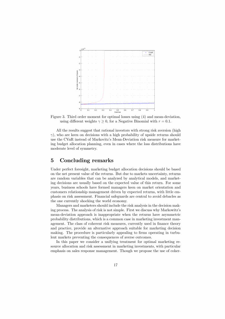
For r = 0.1 the results are even more advantageous for the CVaR than in therelatively more symmetric case considered in Table 2. Figure 3 shows a clearadvantage of the CVaR in terms of third order moment E

h(−Yx∗)3

ifrom the

origin.

16

0 0.1 0.2 0.3 0.4 0.5 0.6 0.7 0.8 0.9 1-9

-8

-7

-6

-5

-4

-3

-2

-1

0x 1014

Gammas

3er o

rder

mom

ent o

f los

ses

CVaRMD

Figure 3. Third order moment for optimal losses using (4) and mean-deviation,using different weights γ ≥ 0, for a Negative Binomial with r = 0.1.

All the results suggest that rational investors with strong risk aversion (highγ), who are keen on decisions with a high probability of upside returns shoulduse the CVaR instead of Markovitz’s Mean-Deviation risk measure for market-ing budget allocation planning, even in cases where the loss distributions havemoderate level of symmetry.

5 Concluding remarksUnder perfect foresight, marketing budget allocation decisions should be basedon the net present value of the returns. But due to markets uncertainty, returnsare random variables that can be analyzed by analytical models, and market-ing decisions are usually based on the expected value of this return. For someyears, business schools have formed managers keen on market orientation andcustomers relationship management driven by expected returns, with little em-phasis on risk assessment. Financial safeguards are central to avoid debacles asthe one currently shocking the world economy.Managers and marketers should include the risk analysis in the decision mak-

ing process. The analysis of risk is not simple. First we discuss why Markowitz’smean-deviation approach is inappropriate when the returns have asymmetricprobability distributions, which is a common case in marketing investment man-agement. The class of coherent risk measures, currently used in finance theoryand practice, provide an alternative approach suitable for marketing decisionmaking. The procedure is particularly appealing to firms operating in turbu-lent markets preventing the consequences of averse outcomes.In this paper we consider a unifying treatment for optimal marketing re-

source allocation and risk assessment in marketing investments, with particularemphasis on sales response management. Though we propose the use of coher-

17

ent risk measures for marketing planning and risk valuation under uncertainty,computing the optimal decision is not simple. Finance theory does not havedeveloped computational methods for solving these problems in general. In thispaper we present a set of first order conditions for the solution, and provide analgorithm for the numerical computation of the optimal decision. We show howthis method can be applied for planning the marketing expenditure with theADBUG sales response model. The results are useful for both marketing andfinance managers, and can be used in a variety of marketing strategic decisions.We have discussed the application of these techniques for budget allocation,

emphasizing sales response to marketing expenditures. But this approach hasa variety of applications, for example firm valuation.Valuations based on expected returns overestimate the actual brand value

compared to the coherent risk measure. For example, brand value can be com-puted as

−ρÃ

nXi=1

Yi

!= E

"nXi=1

Yi

#−D

ÃnXi=1

Yi

!where Yi are net returns from different customers, and n the number of cus-tomers. Firms with high risk levels could have significantly lower brand valuesthan suggested by estimations derived from the expected ROI-CLV, as the rep-resentativeness of the mean can be overstated. Coherence is essential as itguaranties that ρ (

Pni=1 Yi) ≤

Pni=1 ρ (Yi) introducing the classical risk mea-

sure requirement that risk is reduced by increasing our assets, i.e. our customerbase.Finally note that the algorithm covers dynamic problems by using a sce-

nario tree if a "here-and-now" decision is addressed. These ideas can be ex-tended to the case of adaptive decision problems where sequential investmentsare decided with increasing information. In particular, we can consider thatx = (x1, ..., xT ) ∈ X is a sequence of investments in monetary units and in-

troduce the notation xts = (xs, ..., xt) for s ≤ t, andnYx1 , Yx21 , ..., YxT1

ois

the cash-flow of financial returns associated with x (in present values at timezero). If we assume that at time t we have observed the previous outcomesYx1 , Yx21 , ..., Yxt−11

, then we can update the probability function of the invest-

ment value Yx =PT

t=1 Yxt−11. In particular, the multistage investment considers

at each period t the previous decisions xt−11 given, and solves

minxTt ∈Xt(xt−11 )

ρt

ÃTXτ=t

Yxτ−11

!where Xt

¡xt−11

¢=©xTt :

¡xt−11 , xTt

¢ ∈ X :ª , and the conditional CVaR risk mea-sure ρt is defined as

ρt (Y ) = (γ − 1)Et [Y ] + γ ·maxq∈Qt

Et [−Y q]

where Qt =©q ∈ L2 : 0 ≤ q ≤ α−1, Et [q] = 1

ª, and Et [·] denotes the condi-

tional expectation. A discrete scenario tree can be used to adapt the proposed

18

algorithm to this context. Under Markovian assumptions, the conditional ex-pectation can be specified using transition probabilities. Note also that we canexpress the present value of the project as:

V0 = minxTt ∈X

ρ1

ÃYx1 + min

xT2 ∈Xt(x1)ρ2

ÃYx21 + ....+ min

xTT−2∈Xt(xT−21 )ρT

ÃYxT−11

+ minxT∈Xt(xT−11 )

ρT

³YxT1

´!!!.

The project value can be also reconsidered as a variation of the Bellman DynamicPrograming equation, see Ruszynski and Shapiro (2006). We leave the detailsto future research.Summarizing, budget allocation decisions must balance between the ex-

pected profitability and the degree of risk to undertake. Measuring risk isthe first dilemma of a company manager. The CVaR and some other coher-ent risk measures have the ability to differentiate between different sides of riskasymmetries. However, they are not always easy to handle due to the lackof differentiability. By choosing the appropriate risk framework, the presentedalgorithm lead to profitable marketing decision plans with mitigated downsiderisk.

6 References

Artzner, P., F. Delbaen, J. M. Eber, and D. Heath. 1997. Thinking coherently.Risk 10 (November) 68-71.Artzner, P., F. Delbaen, J. M. Eber, and D. Heath. 1999. Coherent measures

of risk. Mathematical Finance 9 (November) 203-228.Bank for International Settlemen. 2006. The new Basel Accord. Basel

Committee on Banking Supervision (http://www.bis.org/publ/bcbs128.htm).Bernoulli, D. 1738. Exposition of a New Theory on the Measurement of Risk.

Comentarii Academiae Scientiarum Imperialis Petropolitanae, as translated andreprinted in 1954, Econometrica, 22 23-36.Blattberg, Robert C. and Stephen J. Hoch. 1990. Database Models and

Managerial Intuition, 50% Model + 50% Manager. Management Science 36(8)887-899.Dickson, P., Giglierano, J.J. 1986. Missing the boat and sinking the boat: a

conceptual model of entrepreneurial risk. Journal of Marketing 50(3) 43-51.Divakar, Suresh, Brian T. Ratchford, and Venkatesh Shankar. 2005. CHAN4CAST:

A Multichannel Multiregion Forecasting Model for Consumer Packaged Goods.Marketing Science 24(3) 333-350.Eisenstein, Eric M. and Leonard M. Lodish. 2002. Precisely Worthwhile or

Vaguely Worthless: Are Marketing Decision Support and Intelligent Systems’Worth It’? Handbook of Marketing, Barton Weitz and Robin Wensley, eds.Sage Publications, London.Global Derivatives Study Group. 1993. Derivatives: Practices and Princi-

ples. Washington D.C.Gupta, Sunil and Thomas J. Steenburgh. 2008. Allocating Marketing Re-

sources, Working Paper 08-069, Harvard Business Review.

19

Hogan, John E., Donald R. Lehmann, Maria Merino, Rajendra K. Srivas-tava, Jacquelyn S. Thomas and Peter C. Verhoef. 2002. Linking customer assetsto financial performance. Journal of Service Research 5(1) 26-38.Holthausen, Duncan M. Gert Assmus. 1982. Advertising Budget Allocation

Under Uncertainty, Management Science, 28, (5), 487-499.Leeflang, Peter S. H., Dick R. Wittink. 2000. Building models for marketing

decisions: Past, present and future. Internat. J. Res. Marketing 17(2—3) 105—126.Little, John D.C. and Leonard M. Lodish. 1969. AMedia Planning Calculus.

Operations Research 17(1) 1-35.Little, John D.C. 1970. Models and Managers: The Concept of Decision

Calculus. Management Science 16(8) B466-B485.Little, John D.C. 1975. BRANDAID: A marketing-mix model: Part 1:

Structure; and Part 2: Implementation, calibration, and case study. OperationsResearch 23(4) 628—673.Little, John D.C. 2004a. Models and Managers: The Concept of a Decision

Calculus. Management Science 50(12) 1841-1853.Little, John D.C. 2004b. Comments on “Models and Managers: The Con-

cept of Decision Calculus. Management Science 50(12) 1854-1860.Lodish, Leonard M. 1971. CALLPLAN: An Interactive Salesman’s Call

Planning System. Management Science 18(4) Part II 25-40.Markowitz, Harry. 1952. Portfolio Selection. The Journal of Finance 7(1)

77—91.Markowitz, Harry M. 1991. Foundations of Portfolio Theory, Journal of

Finance, American Finance Association, vol. 46(2), pages 469-77, June.Natter, Martin, Thomas Reutterer, Andreas Mild, and Alfred Taudes. 2007.

An Assortmentwide Decision-Support System for Dynamic Pricing and Promo-tion Planning in DIY Retailing. Marketing Science 26(4) 576-583.Prakhya, Srinivas, Surendra Rajiv and Kannan Srinivasan. 2006. Risk Aver-

sion and Dynamic Brand Choice. Proceedings of the EMAC, 2006.Rockafellar, R.T.; Uryasev, S. and Zabarankin, M. 2006. Generalized devi-

ation measures in risk analysis. Finance and Stochastics 10 51-74.Rockafellar, R.T. 2007. Coherent approaches to risk in optimization under

uncertainty. Tutorials in Operations Research INFORMS 38-61.Ruszynski, A. and A. Shapiro. 2006. Conditional Risk Mappings. Math.

Oper. Research 31 544-561.Shankar, Venkatesh. 2008. Strategic Allocation of Marketing Resources:

Methods and Managerial Insights. Marketing Science Institute (MSI), Report,08-107.Tirenni, Giuliano, Abderrahim Labbi, Cesar Berrospi, Andre Elisseeff, Timir

Bhose, Kari Pauro, and Seppo Poyhonen. 2007. Customer Equity and LifetimeManagement (CELM) Finnair Case Study. Marketing Science 26(4) 553-565.Tversky, A. and D. Kahneman. 1979. Prospect Theory: An Analysis of

Decisions under Risk. Econometrica 47(2) 263-292von Neumann, J., and Morgenstern, O. 1944. Theory of Games and Eco-

nomic Behavior Harvard University Press, Princeton, N.J.

20

Wang, S. 2000. A class of distortion operators for pricing financial and in-surance risks. Journal of Risk and Insurance 67(1) 15-36.Wierenga, Berend, Gerrit H. Van Bruggen, and Richard Staelin. 1999. The

Success of Marketing Management Support Systems. Marketing Science 18(3)196-207.Wierenga, Berend (ed.). 2008. Handbook of Marketing Decision Models.

Springer, New York.Zhou, Rongrong and Pham, Michel T. 2004. Promotion and prevention

across mental across: When financial products dictate consumer’s investmentgoals. Journal of Consumer Research 31 125-135.

21