Embed Size (px)
DESCRIPTION
Technical Report
Citation preview

ARTIFICIAL IMMUNE SYSTEMS:PART I – BASIC THEORY AND APPLICATIONS
Leandro Nunes de [email protected]
http://www.dca.fee.unicamp.br/~lnunes
Fernando José Von [email protected]
http://www.dca.fee.unicamp.br/~vonzuben
Technical Report
TR – DCA 01/99
December, 1999
Summary
1. INTRODUCTION ...................................................................................................................................................1
1.1 STRUCTURE OF THIS REPORT .................................................................................................................................2
2. THE IMMUNE SYSTEM.......................................................................................................................................3
2.1 A BRIEF HISTORY..................................................................................................................................................4
2.2 ANATOMY OF THE IMMUNE SYSTEM......................................................................................................................6
2.3 THE IMMUNE CELLS ..............................................................................................................................................8
2.3.1 Lymphocytes ................................................................................................................................................9
2.3.2 Phagocytes, Granulocytes and their Relatives ............................................................................................10
2.3.3 The Complement System............................................................................................................................11
2.4 HOW THE IMMUNE SYSTEM PROTECTS THE BODY...............................................................................................11
2.5 THE ANTIBODY MOLECULE.................................................................................................................................13
3. IMMUNE ENGINEERING..................................................................................................................................14
4. AN OVERVIEW OF THE CLONAL SELECTION PRINCIPLE...................................................................16
4.1 REINFORCEMENT LEARNING AND IMMUNE MEMORY..........................................................................................17
4.2 SOMATIC HYPERMUTATION, RECEPTOR EDITING AND REPERTOIRE DIVERSITY..................................................20
4.2.1 The Regulation of the Hypermutation Mechanism............................................................................. ........22
5. REPERTOIRES OF CELLS ................................................................................................................................23
6. PATTERN RECOGNITION................................................................................................................................23
6.1 THE MHC COMPLEX............................................................................................................................................24
6.2 SHAPE-SPACE MODEL .........................................................................................................................................25
6.2.1 Ag-Ab Representations and Affinities........................................................................................................26
7. COGNITIVE ASPECTS OF THE IMMUNE SYSTEM ...................................................................................30
8. IMMUNOLOGIC SELF/NONSELF DISCRIMINATION ...............................................................................32
8.1 NEGATIVE SELECTION .........................................................................................................................................33
8.1.1 Negative T cell Selection............................................................................................................................33
8.1.2 Negative B cell Selection............................................................................................................................34
8.2 POSITIVE SELECTION ............................................................................................................................... ............34
9. IMMUNE NETWORK THEORY ........................................................................................................ ...............35
9.1 IMMUNE NETWORK × NEURAL NETWORKS .........................................................................................................38
9.1.1 Neural Network Approaches to the Immune System and Vice-Versa........................................................39

10. AN EVOLUTIONARY SYSTEM ........................................................................................................................40
11. IMMUNE ENGINEERING TOOLS AND APPLICATIONS...........................................................................41
11.1 DIVERSITY...........................................................................................................................................................41
11.1.1 The Simulated Annealing Approach to Diversity (SAND) ........................................................................42
11.1.2 Related Works ............................................................................................................................................44
11.1.3 Strategy Evaluation.....................................................................................................................................45
11.1.4 Extension to Euclidean Shape-Spaces ........................................................................................................48
11.1.5 Machine-Learning Applications .................................................................................................................50
11.1.6 Discussion...................................................................................................................................................55
11.2 THE ANTIBODY NETWORK (ABNET)..................................................................................................................56
11.2.1 Describing the Network..............................................................................................................................57
11.2.2 Related Networks: Competitive, Hamming, Boolean and Others ..............................................................63
11.2.3 Performance Evaluation..............................................................................................................................66
11.2.4 Discussion...................................................................................................................................................74
11.2.5 Concluding Remarks ..................................................................................................................................75
11.3 AN IMPLEMENTATION OF THE CLONAL SELECTION ALGORITHM.........................................................................76
11.3.1 Model Description ......................................................................................................................................77
11.3.2 Examples of Applications...........................................................................................................................78
11.3.3 Genetic Algorithms × the Clonal Selection Algorithm...............................................................................84
11.3.4 Discussion...................................................................................................................................................85
12. CONCLUDING REMARKS AND FUTURE DIRECTIONS ...........................................................................85
REFERENCES................................................................................................................................................................81
GLOSSARY.....................................................................................................................................................................87
1
ARTIFICIAL IMMUNE SYSTEMS:PART I – BASIC THEORY AND APPLICATIONS
Leandro Nunes de [email protected]
Fernando José Von [email protected]
Technical ReportRT – DCA 01/99December, 1999
AbstractIn the last few years we could perceive a great increase in interest in studying biologically inspired
systems. Among these, we can emphasize artificial neural networks, evolutionary computation,
DNA computation, and now artificial immune systems. The immune system is a complex of cells,
molecules and organs which has proven to be capable of performing several tasks, like pattern
recognition, learning, memory acquisition, generation of diversity, noise tolerance, generalization,
distributed detection and optimization. Based on immunological principles, new computational
techniques are being developed, aiming not only at a better understanding of the system, but also at
solving engineering problems. In this report, after a brief introduction to the immune system,
attaining a relevant level of details when necessary, we discuss the main strategies used by the
immune system to problem solving, and introduce the concept of immune engineering. The immune
engineering makes use of immunological concepts in order to create tools for solving demanding
machine-learning problems using information extracted from the problems themselves. The text is
concluded with the development of several immune engineering algorithms. These tools are
extensively discussed and examples of their applications to artificial and real-world problems are
presented.
1. Introduction
The interest in studying the immune system is increasing over the last few years. Computer
scientists, engineers, mathematicians, philosophers and other researchers are particularly interested
in the capabilities of this system, whose complexity is comparable to that of the brain. A new field
of research called Artificial Immune Systems has arisen (Hunt & Cooke, 1996; Dasgupta, 1997;
McCoy & Devarajan, 1997; Dasgupta, 1999; Hofmeyr & Forrest, 1999; Hofmeyr, 2000), but no
formal general framework was presented yet.

2
Many properties of the immune system (IS) are of great interest for computer scientists and
engineers:
• uniqueness: each individual possesses its own immune system, with its particular
vulnerabilities and capabilities;
• recognition of foreigners: the (harmful) molecules that are not native to the body are
recognized and eliminated by the immune system;
• anomaly detection: the immune system can detect and react to pathogens that the body has
never encountered before;
• distributed detection: the cells of the system are distributed all over the body and, most
importantly, are not subject to any centralized control;
• imperfect detection (noise tolerance): an absolute recognition of the pathogens is not
required, hence the system is flexible;
• reinforcement learning and memory: the system can “learn” the structures of pathogens, so
that future responses to the same pathogens are faster and stronger.
This text is supposed to be a comprehensive overview, keeping a certain level of details, and might
stand for an introductory text to the artificial immune systems and their applications. It presents a
formalism to model receptor molecules and examples of how to use immunological phenomena to
develop engineering and computing tools. The emphasis is on a systemic view of the immune
system, with a focus on the clonal selection principle, the affinity maturation of the immune
response, and the immune network theory.
It is not a matter of concern to us if any mechanism presented here has already been validated
or not, but to discuss how to use these immune mechanisms as powerful sources of inspiration for
the development of computational tools.
A brief introduction to the immune system is followed by the presentation of the concept of
immune engineering, and then a more systemic view of the system is given. This work is concluded
with the development and application of several immune engineering tools.
1.1 Structure of this Report
This report is divided into twelve sections. Section 1 introduces the aims and scope of the report,
and also depicts its structure. In Section 2, a general overview of the immune system is presented,
considering its anatomy and the main cells. Section 3 introduces the immune engineering concept
along with its potential applications. In Section 4, we discuss the clonal selection principle, which
might constitute one of the most important features of the immune response to an antigenic
3
stimulus. A conceptual division of the repertoires of cells is presented in Section 5, and Section 6
addresses the issue of pattern recognition within the immune system. Section 7 discusses some
aspects of the immune cognition, while Section 8 discourses about the self/nonself discrimination
problem and Section 9 reviews the immune network theory. Section 10 poses the immune system as
an evolutionary system and relates the evolution within the immune environment with Darwinian
evolution. Section 11 presents a few immune engineering tools with their machine-learning
applications. This report is concluded, in Section 12, with the final remarks and future directions. A
glossary of biological terms and expressions is also provided, at the end of the report.
2. The Immune System
The immune system (IS) is a complex of cells, molecules and organs that represent an identification
mechanism capable of perceiving and combating dysfunction from our own cells (infectious self)
and the action of exogenous infectious microorganisms (infectious nonself). The interaction among
the IS and several other systems and organs allows the regulation of the body, guaranteeing its
stable functioning (Jerne, 1973; Janeway Jr., 1992).
Without the immune system, death from infection would be inevitable. Its cells and molecules
maintain constant surveillance for infecting organisms. They recognize an almost limitless variety
of infectious foreign cells and substances, known as nonself elements, distinguishing them from
those native noninfectious cells, known as self molecules (Janeway Jr., 1992; Marrack & Kappler,
1993, Mannie, 1999). When a pathogen (infectious foreign element) enters the body, it is detected
and mobilized for elimination. The system is capable of “remembering” each infection, so that a
second exposure to the same pathogen is dealt with more efficiently.
There are two inter-related systems by which the body identifies foreign material: the innate
immune system and the adaptive immune system (Janeway Jr., 1992,1993; Fearon & Locksley,
1996; Janeway Jr. & Travers, 1997; Parish & O’Neill, 1997; Carol & Prodeus, 1998; Colaco, 1998;
Medzhitov & Janeway Jr., 1997a,b,1998).
The innate immune system is so called because the body is born with the ability to recognize
certain microbes and immediately destroy them. Our innate immune system can destroy many
pathogens on first encounter. An important component of the innate immune response is a class of
blood proteins known as complement, which has the ability to assist, or complement, the activity of
antibodies (see Section 2.3.3). The innate immunity is based on a set of receptors encoded in the
germinal centers and known as pattern recognition receptors (PRRs), to recognize molecular
patterns associated with microbial pathogens, called pathogen associated molecular patterns

4
(PAMPs). The PAMPs are only produced by microbes and never by the host organism, hence their
recognition by the PRRs may result in signals indicating the presence of pathogenic agents. This
way, the structures related to the immune recognition must be absolutely distinct from our own cells
and molecules in order to avoid damage to tissues of the host. The consequence of this mechanism
is that the innate immunity is also capable of distinguishing between self and nonself, participating
in the self/nonself discrimination issue, and plays a leading role in the boost of adaptive immunity.
The most important aspect of innate immune recognition is the fact that it induces the
expression of co-stimulatory signals in antigen presenting cells (APCs) that will lead to T cell
activation, promoting the start of the adaptive immune response. This way, adaptive immune
recognition without innate immune recognition may result in the negative selection of lymphocytes
that express receptors involved in the adaptive recognition.
The adaptive immune system uses somatically generated antigen receptors which are clonally
distributed on the two types of lymphocytes: B cells and T cells. These antigen receptors are
generated by random processes and, as a consequence, the general design of the adaptive immune
response is based upon the clonal selection of lymphocytes expressing receptors with particular
specificities (Burnet, 1959-1978). The antibody molecules (Ab) play a leading role in the adaptive
immune system. The receptors used in the adaptive immune response are formed by piecing together
gene segments. Each cell uses the available pieces differently to make a unique receptor, enabling
the cells to collectively recognize the infectious organisms confronted during a lifetime (Tonegawa,
1983). Adaptive immunity enables the body to recognize and respond to any microbe, even if it has
never faced the invader before.
2.1 A Brief History
Immunology is a relatively new science. Its origin is addressed to Edward Jenner, who discovered,
approximately 200 years ago, in 1796, that the vaccinia, or cowpox, induced protection against
human smallpox, a frequently lethal disease (Janeway Jr. & Travers, 1997). Jenner baptized his
process vaccination, an expression that still describes the inoculation of healthy individuals with
weakened, or attenuated samples of agents that cause diseases, aiming at obtaining protection
against these diseases.
When Jenner introduced the vaccination, nothing was known about the ethnological agent of
immunology. In the nineteenth century, Robert Koch proved that infectious diseases were caused by
pathogenic microorganisms, each of which was responsible for a certain pathology.
5
In the 1880 decade, Louis Pasteur designed a vaccine against the chicken-pox and developed
an anti-rage, which was very successful in its first inoculation of a child bitten by a mad dog. So,
many practical triumphs yielded the search for immune protection mechanisms. At that same time,
Elie Metchnikoff discovered phagocytosis and emphasized cellular aspects.
In 1890, Emil von Behring and Shibasaburo Kitasato found that the serum of inoculated
individuals contained substances, called antibodies, that bind specifically to the infectious agents.
Paul Ehrlich was intrigued by the explosive increase in antibody production after exposure to
antigen and attempted to account for this phenomenon by formulating his side-chain theory.
In the early 1900, Jules Bordet and Karl Landsteiner brought to discussion the notion of
immunological specificity. It was shown that the immune system was capable of producing specific
antibodies against artificially synthesized chemicals that had never existed in the world.
The theoretical proposals originated during the period 1930-1950, were mainly sub-cellular. It
was focused the biosynthesis of antibody molecules, made by cells. The conclusion was that the
antigen must bring into the cell information concerning the complementary structure of the antibody
molecule, introducing a theory called template instruction theory. The first well-known works on
the template theory were performed by Breinl and Haurowitz, and further developed and advocated
by the Nobel prize winner Linus Pauling.
The following twenty years, 1950-1970, saw the decline of these early antigen-template
(instructive) theories of antibody formation, in favor of selective theories. The prototype of these
theories was the clonal selection theory, proposed by McFarlane Burnet (1959).
Other Nobel prize winners performed striking theoretical studies, in the period of 1970-1990:
Niels K. Jerne (1974), with his network idea, and Susumu Tonegawa (1983), studying the structure
and diversity of receptors.
In the last few years, most of the work in immunology is focusing on: apoptosis, antigen
presentation, cytokines, immune regulation, memory, autoimmune diseases, DNA vaccines,
intracellular and intercellular signaling, and maturation of the immune response.
Table 1 summarizes the main ideas and researchers in the immunology field. A reader
interested in the history of immunology might refer to Jerne (1974), Bell & Perelson (1978), and
Cziko (1995).

6
Table 1: History of immunology (adapted from Jerne, 1974).
Aims Period Pioneers Notions
1796-1870 JennerKoch
ImmunizationPathology
Application1870-1890 Pasteur
MetchinikoffImmunizationPhagocytosis
1890-1910 von Behring & KitasatoEhrlich
AntibodiesCell receptors
Description1910-1930 Bordet
LandsteinerSpecificityHaptens
1930-1950 Breinl & HaurowitzLinus Pauling
Antibody synthesisAntigen templateMechanisms
(System) 1950-1980 BurnetNiels Jerne
Clonal selectionNetwork and Cooperation
Molecular 1980-1990 Susumu Tonegawa Structure and diversity of receptors
2.2 Anatomy of the Immune System
The tissues and organs that compose the immune system are distributed throughout the body. They
are known as lymphoid organs, once they are related to the production, growing and development
of lymphocytes, the leukocytes that compose the main operative part of the immune system. In the
lymphoid organs, the lymphocytes interact with important non-lymphoid cells, either during their
maturation process or during the start of the immune response. The lymphoid organs can be divided
into primary (or central), responsible for the production of new lymphocytes, and secondary (or
peripheral) where the lymphocyte repertoires meet the antigenic universe.
The lymphoid organs, and their main functions, include (see Figure 1):
• tonsils and adenoids: specialized lymph nodes containing immune cells that protect the body
against invaders of the respiratory system;
• lymphatic vessels: constitute a network of channels that transport the lymph (fluid that
carries lymphatic cells and exogenous antigens) to the immune organs and blood;
• bone marrow: soft tissue contained in the inside part of the longest bones, responsible for
the generation of the immune cells;
7
Lymphatic vessels
Lymphnodes
Thymus
Spleen
Tonsils andadenoids
Bone marrow
Appendix
Peyer’s patches
Figure 1: Anatomy of the immune system (lymphoid organs)
• lymph nodes: act as convergence sites of the lymphatic vessels, where each node stores
immune cells, including B and T cells (site where the adaptive immune response takes
place);
• thymus: a few cells migrate into the thymus, from the bone marrow, where they multiply and
mature, transforming themselves into T cells, capable of producing an immune response;
• spleen: site where the leukocytes destroy the organisms that invaded the blood stream;
• appendix and Peyer’s patches: specialized lymph nodes containing the immune cells
destined to protect the digestive system.
The immune system’s architecture is intrinsically multi-layered, with defenses spread about several
levels (see Figure 2). The protection layers can be divided as follows (Janeway Jr. & Travers, 1997;
URL 1; Rensberger, 1996; Hofmeyr, 1997,2000):
• physical barriers: our skin works as a shield to the body’s protection against invaders, either
malefic or not. The respiratory system also helps in keeping the antigens away. Its defenses
include the trapping irritants in nasal hairs and mucus, carrying mucus upward and outward
on cilia, coughing and sneezing. The skin and the mucous membranes lining the respiratory
and digestive tracts also contain macrophages and antibodies.
• physiologic barriers: fluids such as saliva, sweat and tears contain destructive enzymes.
Stomach acids kill most microorganisms ingested in food and water. The pH and
temperature of the body present unfavorable life conditions for some invaders.

8
Phagocyte
Adaptiveimmune
response
Lymphocyte
Innateimmune
response
Physiologicalconditions
Skin
Pathogens
Figure 2: Multi-layer structure of the immune system
• innate immune system and adaptive immune system: see previous section for brief
descriptions.
2.3 The Immune Cells
The immune system is composed of a great variety of cells that are originated in the bone marrow,
where plenty of them mature. From the bone marrow, they migrate to patrolling tissues, circulating
in the blood and lymphatic vessels. Some of them are responsible for the general defense, whereas
others are “trained” to combat highly specific pathogens. For an efficient functioning, it is necessary
a continuous cooperation among the agents (cells). Figure 3 presents a structural division among the
cells and secretions produced by the immune system.
B ce lls an dA n tib od ies
T ce lls an dL ym p h ok in es
N atu ra l K ille r C e lls(N K )
L ym p h oc ytes P h ag ocytes , g ran u loc ytes an dth eir re la tives
C om p lem en t
C e lls an d S ecret ion s
Figure 3: Structural division of the cells and secretions of the immune system
9
2.3.1 Lymphocytes
Lymphocytes are small leukocytes that possess a major responsibility in the immune system. There
are two main types of lymphocytes: B lymphocyte (or B cell), which, upon activation, differentiate
into plasmocyte (or plasma cells) capable of secreting antibodies; and T lymphocyte (or T cell).
Most of the lymphocytes is formed by small resting cells, which only exhibit functional
activities after some kind of interaction with the respective antigens, necessary for proliferation an
specific activation. The B and T lymphocytes express, on their surfaces, receptors highly specific
for a given antigenic determinant. The B cell receptor is a form of the antibody molecule bound to
the membrane, and which will be secreted after the cell is appropriately activated.
B cells and antibodies
The main functions of the B cells include the production and secretion of antibodies (Ab) as a
response to exogenous proteins like bacteria, viruses and tumor cells. Each B cell is programmed to
produce a specific antibody. The antibodies are specific proteins that recognize and bind to another
particular protein. The production and binding of antibodies is usually a way of signaling other cells
to kill, ingest or remove the bound substance.
As the antibody molecule represents one of the most important recognition devices of the
immune system, it will be discussed separately in Section 2.5.
T cells and lymphokines
The T cells are so called because they mature within the thymus (Dreher, 1995). Their function
include the regulation of other cells’ actions and directly attack the host infected cells. The T
lymphocytes can be subdivided into three major subclasses: T helper cells (Th), cytotoxic (killer) T
cells and suppressor T cells.
The T helper cells, or simply Th cells, are essential to the activation of the B cells, other T
cells, macrophages and natural killer (NK) cells. They are also known as CD4 or T4 cells.
The killer T cells, or cytotoxic T cells, are capable of eliminating microbial invaders, viruses or
cancerous cells. Once activated and bound to their ligands, they inject noxious chemicals into the
other cells, perforating their surface membrane and causing their destruction.
The suppressor T lymphocytes are vital for the maintenance of the immune response. They are
sometimes called CD8 cells, and inhibit the action of other immune cells. Without their activity,
immunity would certainly loose control resulting in allergic reactions and autoimmune diseases
(Janeway Jr. & Travers, 1997).

10
The T cells work, primarily, by secreting substances, known as cytokines or, more specifically,
lymphokines and their relatives, the monokines produced by monocytes and macrophages. These
substances constitute powerful chemical messengers. The lymphokines promote cellular growth,
activation and regulation. In addition, lymphokines can also kill target cells and stimulate
macrophages.
Natural killer cells
The natural killer cells (NK) constitute another kind of lethal lymphocytes. Like the killer T cells,
they contain granules filled with powerful chemicals. They are designated natural killers because,
unlike the killer T cells, they do not need to recognize a specific antigen before they start acting.
They attack mainly tumors and protect against a great variety of infectious microbes. These cells
also contribute to the immune regulation, secreting large amounts of lymphokines.
2.3.2 Phagocytes, Granulocytes and their Relatives
The phagocytes (literally “cell eaters”) are white blood cells capable of ingesting and digesting
microorganisms and antigenic particles. Some phagocytes also have the ability to present antigens
to lymphocytes, thus being called antigen presenting cells (APCs).
Important phagocytes are the monocytes and the macrophages. The monocytes circulate
through the blood and migrate into the tissues, where they become macrophages (“big eaters”). The
macrophages are versatile cells that perform several functions. They present antigens to T
lymphocytes, after ingesting and digesting them. They play an important role at the beginning of the
immune response.
The neutrophils and eusinophils are also phagocytes with functions similar to those of the
macrophages. The basophils are found in the blood stream and are similar to the mast cells, though
they derive from a separate lineage. They are important to allergic responses and contain granules
filled with powerful chemicals. These chemicals destroy microorganisms, contributing to the
inflammatory reaction. Figure 4 illustrates the most important phagocytes.
Monocyte
MacrophageNeutrophil
EusinophilMast cell
Basophil
Figure 4: Phagocytic cells
11
2.3.3 The Complement System
The complement system constitutes a complex formed by a set of circulating plasma proteins that
complement the function of the antibodies. When the complement detects an invader organism, each
of its components promotes a chain reaction (complement cascade). The result is a complex of
proteins that bind to the surface of the invader causing lesions on its protecting membrane or
facilitating the operation of phagocytes. It is formed by approximately 25 proteins that circulate
inactively all over the body. Figure 5 illustrates the complement chain reaction.
AntigenAntibody (Ig)
Cellswells
andbursts
Complexinserted in cellwall
Complement(cascade)
Firstcomplementprotein
Figure 5: Complement activation (cascade reaction)
2.4 How the Immune System Protects the Body
As discussed previously, our body is protected by a diverse army of cells and molecules that work
in concert, where the ultimate target of all immune responses is an antigen (Ag), which is usually a
foreign molecule from a bacterium or other invader. Figure 6 presents a simplified version of the
basic immune mechanisms of defense.
Specialized antigen presenting cells (APCs), such as macrophages, roam the body, ingesting
and digesting the antigens they find and fragmenting them into antigenic peptides (Nossal, 1993)
(I). Pieces of these peptides are joined to major histocompatibility complex (MHC) molecules and
are displayed on the surface of the cell. Other white blood cells, called T cells or T lymphocytes,
have receptor molecules that enable each of them to recognize a different peptide-MHC
combination (II). T cells activated by that recognition divide and secrete lymphokines, or chemical
signals, that mobilize other components of the immune system (III). The B lymphocytes, which also

12
have receptor molecules of a single specificity on their surface, respond to those signals. Unlike the
receptors of T cells, however, those of B cells can recognize parts of antigens free in solution,
without MHC molecules (IV). When activated, the B cells divide and differentiate into plasma cells
that secrete antibody proteins, which are soluble forms of their receptors (V). By binding to the
antigens they find, antibodies can neutralize them (VI) or precipitate their destruction by
complement enzymes or by scavenging cells. Some T and B cells become memory cells that persist
in the circulation and boost the immune system’s readiness to eliminate the same antigen if it
presents itself in the future. Because the genes for antibodies in B cells frequently suffer mutation
and editing, the antibody response improves after repeated immunizations, this phenomenon is
called affinity maturation and will be discussed further in the text.
APC
MHC protein Antigen
Peptide
T cell
Activated T cell
B cell
Lymphokines
Activated B cell(Plasma cell)
( I )
( II )
( III )
( IV )
( V )
( VI )
Figure 6: How the immune system defends the body
13
2.5 The Antibody Molecule
Through the recognition and distinction of specific molecular patterns, the antibodies play a central
role in the immune system. Antigens are diverse in structure, forcing the antibody repertoire to be
large (Tonegawa, 1983). The genetic information necessary to code for this exceedingly large
number of different, but related, proteins is stored in the genome of a germ-line cell and transmitted
through generations.
The basic unit of an antibody (Ab), or immunoglobulin (Ig), molecule is composed of two
identical light (L) chains and two identical heavy (H) chains (Tonegawa, 1983,1985; Janeway Jr. &
Travers, 1997, Perelson & Weisbuch, 1997). The variable region, or V-region, is primarily
responsible for antigen recognition and contains particularly variable subregions whose residues
have been implicated in actual antigen contact. These subregions are referred to as
complementarity-determining regions (CDRs). The constant regions (C) are responsible for a
variety of effector functions, such as complement fixation (see Figure 7(a)). It was found that an
immunoglobulin polypeptide chain is encoded in multiple gene segments scattered along a
chromosome of the germ-line genome. These gene segments must be brought together to form a
complete immunoglobulin gene active in B lymphocytes. In addition, mutations are introduced
somatically into an immunoglobulin gene at a high rate (hypermutation). Both, the recombination
and mutation increase greatly the diversity of the genetic information carried in the germ-line
genome.
Antigen binding sitesVH
VL
CH CH
VL
CL
CH
VH
CH
CL
... ... ... V V
V library
D D
D library
J J
J library
Gene rearrangement
V D J Rearranged DNA
(a) (b)Figure 7: Antibody molecule and its genome. (a) Variable region (V-region) responsible for antigenrecognition and constant region (C-region) responsible for a variety of effector functions, like complementfixation. (b) The rearrangement processes that leads to the formation of the variable region of the heavychain (VH) of an antibody molecule: the gene fragments (exactly one from each gene library) areconcatenated in an orderly manner. The resulting product is then translated into the functional antibodymolecule. V, D, J are individual libraries that contribute to the production of the immune receptors.

14
The presence of both combinatorial recombination and somatic mutation as mechanisms for the
diversification of antibody genes is intriguing (Tonegawa, 1985). Why have two systems evolved to
accomplish the same task? Both mechanisms are under strict control during the development of B
cells. The recombination of the immunoglobulin gene segments is performed first, and it is
complete by the time the cells are first exposed to antigens. It creates a population of cells that vary
widely in their specificity, from which a few cells are compatible with some given antigen. The
mutational mechanism is then called into action during the proliferation of the selected B cell
clones. By altering individual nucleotide bases, the mutations fine-tune the immune response,
creating immunoglobulin genes whose products better match the antigen. In Section 4.2, it will be
discussed the somatic hypermutation and receptor editing (or V(D)J recombination) mechanisms,
responsible for fine-tuning lymphocyte receptors during an immune response.
Receptor diversity is generated during lymphocyte development by random combinatorial
joining of antigen receptor gene fragments (Tonegawa, 1983). B and T lymphocytes somatically
rearrange the V, D and J elements of their immunoglobulin and T cell receptor (TCR) genes to
create a vast array of different clones of B and T lymphocytes that express distinct antigen receptors
(see Figure 7(b) for illustration).
3. Immune Engineering
In this section, we intend to introduce the concept of immune engineering and briefly discuss its
relation with the artificial immune systems.
Nowadays, most of the technological solutions available are based upon a strict set of plans, or
rules, which specify a detailed group of steps to be followed by each of their component parts. The
overall behavior is usually simple enough to be predicted and studied. In other words, the problem
of engineering consists in designing a basic system to perform a particular task, whereas the
conventional approaches systematically devise detailed step-by-step procedures. This approach can
not provide the most efficient treatment for complex engineering problems, demanding the
emergence of new paradigms.
The capabilities of natural systems go far beyond those of any conventional technological
means. The elucidation and application of a set of general principles that govern the overall
behavior of these natural systems may lead to new forms of engineering (Wolfram, 1986). Nature
provides many examples of systems with simple basic components, in which a collective
competition and cooperation turns out to an extremely complex overall behavior, e.g., insects
colonies (like ants), the immune system, etc. One of the most striking characteristics of such
15
systems is their robustness, expressed as a high tolerance to small perturbations to individual
components. This robustness underlies the principles of distribution, where small pieces by
themselves are not “deadly” significant to the whole, but when these pieces are put together as an
ensemble of individuals (or agents), very complex behaviors can emerge.
Ideas gleaned from natural systems, like immunology or neurobiology, can and are being used
to engineer (or design) systems whose complex behavior can be controlled and dedicated to
particular tasks. The immune system, in its potentiality to solve pattern recognition tasks, is robust,
once small changes in the form of a pattern (pathogen) may still lead to a particular response (cross-
reactivity).
Conventional engineering techniques usually require detailed specification of the precise
behavior of each of the components of the systems. On the other hand, the new engineering
paradigm (immune engineering) demands only general, or approximate, specification of some
aspects of the overall behavior of the system, like a performance measure or a fitness function.
As discussed in the introduction, another emerging field is the so called Artificial Immune
System (AIS). We suggest that the AIS might represent those strategies that try to model somehow
any specific immunological mechanism aiming at providing a better understanding of the biological
phenomenon. On the other hand, immune engineering (IE) represents all approaches that use
immune inspiration to develop engineering or computational tools. The idea is to use information
contained in the problem itself in order to solve it. Nevertheless, it is not our intention to pose a
strict limit between the AIS and the IE. Instead, we intend to make use of all immunologically
inspired phenomena and algorithm in order to solve complex problems. The topics involved in the
definition and development of the immune engineering cover mainly:
• hybrid structures and algorithms that take into account immune-like mechanisms;
• computational algorithms based on immunological principles, like distributed processing,
clonal selection algorithms, and immune network theory;
• immunity-based optimization, learning, self-organization, artificial life, cognitive models,
multi-agent systems, design and scheduling, pattern recognition and anomaly detection; and
• artificial immune systems and their applications.
Potential applications of the immune engineering can be listed (but are not limited to): pattern
recognition, function approximation and optimization, anomaly detection, computer and network
security, generation of diversity and noise tolerance.

16
4. An Overview of the Clonal Selection Principle
The clonal selection principle, or theory, is the algorithm used by the immune system to describe
the basic features of an immune response to an antigenic stimulus. It establishes the idea that only
those cells that recognize the antigens proliferate, thus being selected against those which do not.
Clonal selection operates on both T cells and B cells.
The immune response occurs inside the lymph nodes (Weissman & Cooper, 1993) and the
clonal expansion of the lymphocytes occurs within the germinal centers (GCs), in the follicular
region of the white pulp, which is rich in antigen presenting cells (Tarlinton, 1998).
When an animal is exposed to an antigen, some subpopulation of its bone marrow’s derived
cells (B lymphocytes) respond by producing antibodies. Each cell secretes only one kind of
antibody, which is relatively specific for the antigen. By binding to these immunoglobulin
receptors, with a second signal from accessory cells, such as the T-helper cell, an antigen stimulates
the B cell to proliferate (divide1) and mature into terminal (non-dividing) antibody secreting cells,
called plasma cells. While plasma cells are the most active antibody secretors, large B lymphocytes,
which divide rapidly, also secrete Ab, albeit at a lower rate. While B cells secrete Ab, T cells do not
secrete antibodies, but play a central role in the regulation of the B cell response and are preeminent
in cell mediated immune responses (see Figure 6 – Section 2.4). Lymphocytes, in addition to
proliferating or differentiating into plasma cells, can differentiate into long-lived B memory cells.
Memory cells circulate through the blood, lymph and tissues, probably not manufacturing
antibodies (Perelson et al., 1978), but when exposed to a second antigenic stimulus commence
differentiating into large lymphocytes capable of producing high affinity antibody, preselected for
the specific antigen that had stimulated the primary response. Figure 8 depicts the clonal selection
principle.
The main features of the clonal selection theory are (Burnet, 1978):
• the new cells are copies of their parents (clone) subjected to a mutation mechanism with
high rates (somatic hypermutation);
• elimination of newly differentiated lymphocytes carrying self-reactive receptors;
• proliferation and differentiation on contact of mature cells with antigens; and
• the persistence of forbidden clones, resistant to early elimination by self-antigens, as the
basis of autoimmune diseases.
1 The various cell divisions (mitosis) generate a clone, i.e., a set of cells that are the progeny of a single cell.
17
Proliferation(Cloning)
Differentiation
Plasma cells
Memory cellsSelection
Antigens
M
M
Figure 8: The clonal selection principle. Small resting B cells created in the bone marrow each carry adifferent receptor type defined by their VH and VL regions (see Figure 7 – Section 2.5). Those cells carryingreceptors specific for the antigen, proliferate and differentiate into plasma and memory cells.
The analogy with natural selection (Holland, 1995) should be obvious, the fittest clones being the
ones that best recognize antigen or, more precisely, the ones that are triggered best. For this
algorithm to work, the receptor population or repertoire, has to be diverse enough to recognize any
foreign shape. A mammalian immune system contains an heterogeneous repertoire of
approximately 1012 lymphocytes in human (Perelson et al., 1976), and a resting (unstimulated) B
cell may display around 105–107 identical antibody-like receptors (Jerne, 1984). The repertoire is
believed to be complete, which means that it can recognize any shape. We will discuss a few
classifications for the repertoire of cells, along with their completeness, in Section 5.
4.1 Reinforcement Learning and Immune Memory
In order to be protective, antigen recognition is not enough, the immune system must also have
sufficient resources to mount an effective response against pathogens. As in typical predator-prey
situations, the size of the lymphocyte subpopulation specific for the pathogen (clone), with relation
to the size of the pathogen population, is crucial to determining the outcome of infection. Learning
in the immune system involves raising the population size and affinity of those lymphocytes that
have proven themselves to be valuable by having recognized some antigen. Because the total
number of lymphocytes in the immune system is regulated, increases in the sizes of some clones
mean that other clones may have to decrease in size. However, the total number of lymphocytes is
not kept absolutely constant. If the immune system learns only by increasing the population sizes of
specific lymphocytes, it must either “forget” previously learned antigens, increase in size, or

18
constantly decrease the portion of its repertoire that is generated at random and responsible for
responding to novel antigens (Perelson & Weisbuch, 1997).
In the normal course of the evolution of the immune system, an organism would be expected to
encounter a given antigen repeatedly during its life time. The initial exposure to an antigen that
stimulates an adaptive immune response (an immunogen) is handled by a spectrum of small clones
of B cells, each producing antibodies of different affinity. The effectiveness of the immune response
to secondary encounters could be considerably enhanced by storing some high affinity antibody
producing cells from the first infection (memory cells), so as to form a large initial clone for
subsequent encounters (Ada & Nossal, 1987). Rather than ‘starting from scratch’ every time, such a
strategy would ensure that both the speed and accuracy of the immune response becomes
successively greater after each infection (Perelson et al., 1978, Farmer et al., 1986). This scheme is
intrinsic of a reinforcement learning strategy (Sutton & Barto, 1998), where the system is
continuously improving its capability to perform its task. In the next section, it will be introduced
some mechanisms through which the B cells become increasingly more specialized. Meanwhile, we
will continue discussing the outcomes of these mechanisms.
To illustrate the immune response (memory), consider that an antigen A is introduced at time
zero and it finds a few specific antibodies inside the animal. After a lag phase, the Ab against
antigen A appears and its concentration rises up to a certain level, and then starts to decline
(primary response). When another antigen B is introduced, no antibody is present, showing the
specificity of the antibody response (Janeway Jr. & Travers, 1997). On the other hand, one
important characteristic of the immune memory is that it is associative: B cells adapted to a certain
type of antigen A presents a faster and more efficient secondary response not only to A, but also to
any structurally related antigen B. This phenomenon is called immunological cross-reaction, or
cross-reactive response (Hoffman, 1986; Ada & Nossal, 1987; Sprent, 1994; Smith et al., 1997;
Hodgkin, 1998; Mason, 1998). This associative memory is contained in the process of vaccination
and is called generalization capability, or simply generalization, in other artificial intelligence
fields, like neural networks (Haykin, 1999). Figure 9 illustrates primary, secondary and cross-
reactive responses.
Some characteristics of the associative memories are particularly interesting in the immune
engineering context:
• the data stored is recovered through the reading of the same or related data;
• they are usually robust, not only to noise in the data, but also to failures in the components
of the memory.
19
By comparison with the primary response, the secondary response is characterized by a shorter
lag phase, a higher rate, and longer persistence of antibody synthesis. Moreover, a dose of antigen
substantially lower than that required to initiate a primary response can cause a secondary response.
Some authors (Allen et al., 1987; Countinho, 1989) suggested that long-lived B cells which
have responded to an antigenic previous exposure remain in a small, resting state and will play an
important role in secondary antibody responses. These memory cells are disconnected, at least
functionally, from the other cells, and memory is a clonal property, at least in the context of
secondary responses. Sprent (1994) argued that whether memory cells are truly resting cells is a
debatable issue and suggested that typical memory cells are semi-activated cells engaged in low-
grade responses to persisting antigens.
It is important to remark that, under an engineering perspective, the cells with highest affinity
must be preserved somehow as high quality candidate solutions, and shall only be replaced by
improved candidates, based on statistical evidences.
As a summary, immune learning and memory are acquired through (Ahmed & Sprent, 1999):
• repeated exposure to a pathogen;
• affinity maturation of the receptor molecules (see next section);
• low-grade chronic infection;
• cross-reactivity to endogenous and exogenous pathogens; and
• idiotypic networks (see Section 8).
Antigen A AntigensA + B
Primary Response SecondaryResponse
lag
Response toantigen A
Responseto antigen B
Antib
ody
conc
entra
tion
Days
lag
Figure 9: Primary, secondary and cross-reactive immune responses. After an antigen has been seen once(primary response), subsequent encounters with the same antigen, or a related one (cross-reaction), will leadto a faster and stronger response (secondary response).

20
4.2 Somatic Hypermutation, Receptor Editing and Repertoire Diversity
In a T cell dependent immune response, the repertoire of antigen-activated B cells is diversified
basically by two mechanisms: hypermutation and receptor editing (Tonegawa, 1983, 1985; Berek &
Ziegner, 1993; Nussenzweig, 1998; George & Gray, 1999). Only high-affinity variants are selected
into the pool of memory cells. This maturation process takes place in a special micro environment
called germinal center (GC) (Nossal, 1992; Tarlinton, 1998).
Antibodies present in a memory response have, on average, a higher affinity than those of the
early primary response. This phenomenon, which is restricted to T-cell dependent responses, is
referred to as the maturation of the immune response. This maturation requires that the antigen-
binding sites of the antibody molecules in the matured response be structurally different from those
present in the primary response. Three different kinds of mutational events have been observed in
the antibody V-region (Allen et al., 1987):
• point mutations;
• short deletions; and
• non-reciprocal exchange of sequence following gene conversion (repertoire shift).
Random changes are introduced into the variable region genes and occasionally one such change
will lead to an increase in the affinity of the antibody. It is these higher-affinity variants which are
then selected to enter the pool of memory cells. Not only the repertoire is diversified through a
hypermutation mechanism but, in addition, mechanisms must exist such that rare B cells with high
affinity mutant receptors can be selected to dominate the response. Due to the random nature of the
somatic mutation process, a large proportion of mutating genes become non-functional or develop
harmful anti-self specificities (Storb, 1998). Those cells with low affinity receptors, or the self-
reactive cells, must be efficiently eliminated (or become anergic) so that they do not significantly
contribute to the pool of memory cells (Berek & Ziegner, 1993; Adams, 1996; Nussensweig, 1998;
George & Gray, 1999). How B cells with compromised antigen binding abilities are eliminated is
not fully understood. Apoptosis in the germinal centers is likely (Coutinho, 1989; Nossal, 1992).
Apoptosis is a subtle cell death process, often equated with programmed cell death (McConkey et
al., 1990; Cohen, 1993).
The analysis of the development of the antibody repertoire expressed on B cells in the germinal
center has clearly demonstrated the key role that these structures play in the maturation of the
immune response. Both processes are of vital importance for the maturation – hypermutation of the
variable region and selection of higher-affinity variants. The increase in antibody affinity from the
21
primary to the secondary response, and so on, shows that maturation of the immune response is a
continuous process (reinforcement learning – see previous section).
There are three essential features of adaptive immune responses: sufficient diversity to deal
with a universe of antigens, discrimination of self from non-self, and long lasting immunologic
memory. In the original clonal selection theory, proposed by Burnet (1959), memory would be
provided by expanding the size of an antigen-specific clone, and random mutation would be
allowed to enhance affinity. Furthermore, self-reactive cells would be clonally deleted during
development. Recent results suggest that the immune system practices molecular selection of
receptors in addition to clonal selection of lymphocytes (Nussenzweig, 1998). Instead of the
expected clonal deletion of all self-reactive cells, occasionally B lymphocytes were found that had
undergone receptor editing: these B cells had deleted their self-reactive receptors and developed
entirely new receptors by V(D)J recombination (see Figure 7, p. 13). Although editing and receptor
selection were not part of Burnet’s model, the clonal selection theory could certainly accommodate
receptor editing if receptor selection occurred before cellular selection (see Section 4). Any high
affinity clone developed by somatic hypermutation or editing, would be expected to be
preferentially expanded, but a few low affinity cells are also allowed to enter the repertoire,
maintaining the population diversity.
In Section 4, we presented Tonegawa’s (1985) point of view for the necessity of the use of two
different mechanisms to introduce diversity during an immune response. George & Gray (1999)
argued why should there be an additional diversity introducing mechanism during the process of
affinity maturation, and suggested that receptor editing offers the ability to escape from local
optima on an affinity landscape. Figure 10 illustrates this idea by considering all possible antigen-
binding sites depicted in the x-axis, with the most similar ones adjacent to each other. The Ag-Abaffinity is shown on the y-axis. If it is taken a particular antibody (A) selected during a primary
response, then point mutations allow the immune system to explore local areas around A by making
small steps towards an antibody with higher affinity, leading to a local optima (A1). Because
mutations with lower affinity are lost, the Ab can not go down the hill. Receptor editing allows an
antibody to take large steps through the landscape, landing in a locale where the affinity might be
lower (B). However, occasionally the leap will lead to an antibody on the side of a hill where the
climbing region is more promising (C), reaching the global optimum. From this locale, point
mutations can drive the Ab to the top of the hill (C1). In conclusion, point mutations are good for
exploring local regions, while editing may rescue immune responses stuck on unsatisfactory local
optima.

22
Antigen-binding sites
Affin
ity A
A1
C1
C
B
B1
Figure 10: Schematic representation of shape-space for antigen-binding sites. Somatic mutations allow thereach of local optima, while receptor editing introduces diversity, leading to possible new candidatereceptors.
Receptor editing and point mutations play complementary roles in the affinity maturation process.
In addition to somatic hypermutation and receptor editing, a fraction of newcomer cells from the
bone marrow is added to the lymphocyte pool in order to maintain the diversity of the population.
According to Jerne (1984), from 5-8% of the least stimulated lymphocytes are replaced per cell
generation, joining the pool of available antigen recognizing cells. This may yield the same result as
the process of receptor editing, i.e., a broader search for the global optimum.
4.2.1 The Regulation of the Hypermutation Mechanism
A hypermutation mechanism with a rate close to 1 × 10⁻³ per base pair (bp) of the variable regions,
per generation, operates selectively during the cell differentiation process. Since the combined
length of these variable regions is around 700bp, on average one mutation per cell division will be
introduced (Allen et al., 1987; Berek & Ziegner, 1993; Perelson & Weigel, 1998).
A rapid accumulation of mutations is necessary for a fast maturation of the immune response,
but the majority of the changes will lead to poorer or non-functional antibodies. If a cell that has
just picked up a useful mutation continues to be mutated at the same rate during the next immune
responses, then the accumulation of deleterious changes may cause the loss of the advantageous
mutation. Thus, a short burst of somatic hypermutation, followed by a breathing space to allow for
selection and clonal expansion, may form the basis of the maturation process. The selection
mechanism may provide a means by which the regulation of the hypermutation process is made
dependent on receptor affinity. Cells with low affinity receptors may be further mutated and, as a
rule, die through apoptosis. In cells with high-affinity antibody receptors however, hypermutation
may be inactivated (Kepler & Perelson, 1993a,b).
23
5. Repertoires of Cells
For each of the two main types of cellular components in the lymphoid system (B and T cells) we
can consider three classes of repertoires (Jerne, 1974; Coutinho et al., 1984; DeBoer &
Perelson, 1991; Perelson & Weisbuch, 1997; Storb, 1998):
• the potential repertoire, determined by the number, structure and mechanisms of expression
of germ-line collections of genes encoding antibodies or T cell receptors, plus the possible
somatic variants derived from these (errors introduced during gene segment joining);
• the available (or expressed) repertoire defined as the set of diverse molecules that are used
as lymphocyte receptors, that is, what can be (but is not at present being) used;
• the actual repertoire, that set of antibodies and receptors produced by effector lymphocytes
activated in the internal environment which actually participate in the interactions defining
the autonomous activity in any given state.
The immune system in its ability to recognize antigens is complete. The antibody molecules and
T cell receptors produced by the lymphocytes of an animal can recognize any foreign (or self)
molecule, even those artificially synthesized. Antibody molecules have immunogenic idiotopes. It
follows from the completeness axiom that these will be recognized by other antibody molecules.
This argument leads to the concept of idiotypic networks that will be discussed later. The main
factors that result in the repertoire completeness are its diversity (obtained by mutation, editing and
gene rearrangement) its cross-reactivity and its multi-specificity (Inman, 1978; Perelson & Oster,
1979; Tonegawa, 1983; Coutinho et al., 1984; Jerne, 1985; Varela et al., 1988). Cross-reactivity
along with multi-specificity are the main reasons why a lymphocyte repertoire smaller than the
possible antigen set to be recognized can succeed on its task: pathogen recognition and elimination
(Inman, 1978; Hodgkin, 1998; Mason, 1998). The difference between cross-reactivity and multi-
specificity is that the former indicates the recognition of related antigenic patterns (or epitopes),
while the latter refers to the recognition of very different chemical structures (Perelson &
Weisbuch, 1997).
6. Pattern Recognition
From the point of view of pattern recognition in the immune system, the most important feature of
both B and T cells is that they have receptor molecules on their surfaces that can recognize antigens
(either free or bound to an MHC molecule). In the B cells case, the receptor is an immunoglobulin,
or antibody, molecule (see Section 2.5) embedded in the membrane of the cell.
24
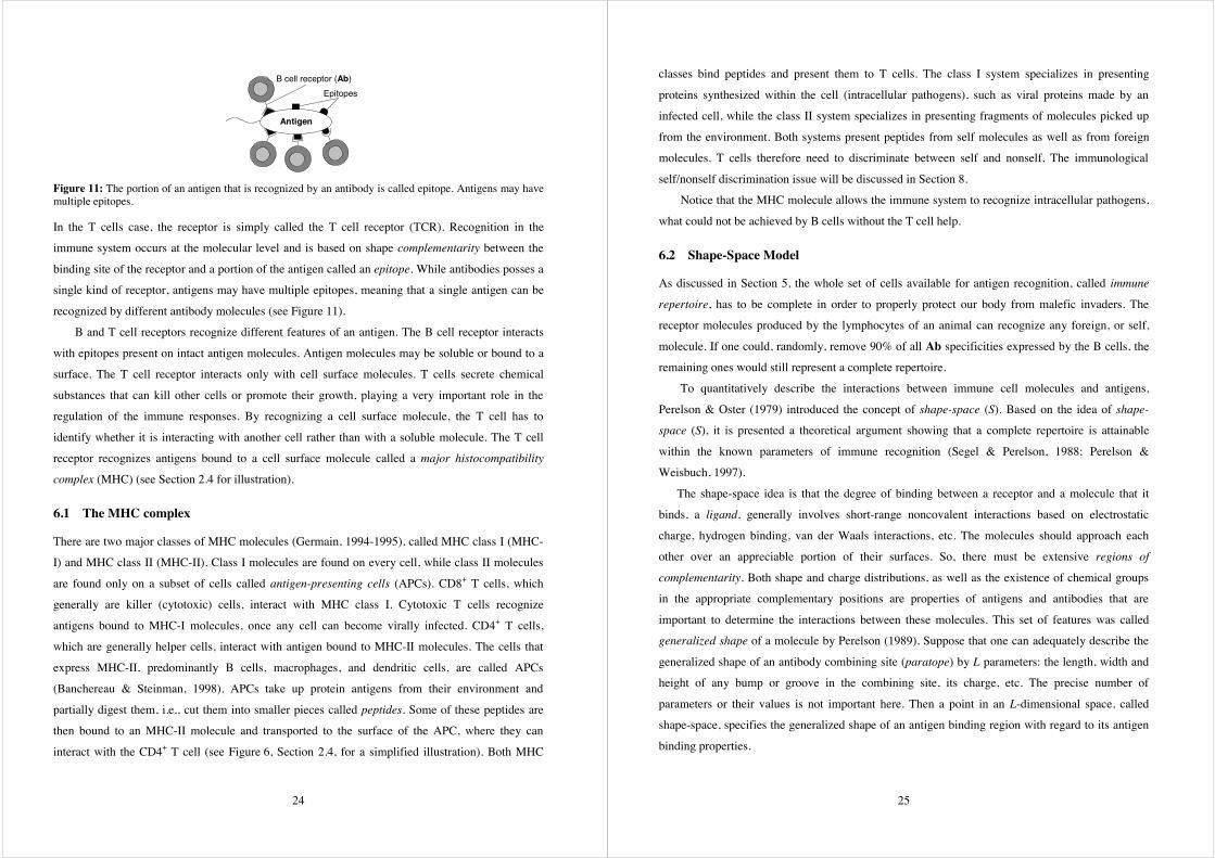
EpitopesB cell receptor (Ab)
Antigen
Figure 11: The portion of an antigen that is recognized by an antibody is called epitope. Antigens may havemultiple epitopes.
In the T cells case, the receptor is simply called the T cell receptor (TCR). Recognition in the
immune system occurs at the molecular level and is based on shape complementarity between the
binding site of the receptor and a portion of the antigen called an epitope. While antibodies posses a
single kind of receptor, antigens may have multiple epitopes, meaning that a single antigen can be
recognized by different antibody molecules (see Figure 11).
B and T cell receptors recognize different features of an antigen. The B cell receptor interacts
with epitopes present on intact antigen molecules. Antigen molecules may be soluble or bound to a
surface. The T cell receptor interacts only with cell surface molecules. T cells secrete chemical
substances that can kill other cells or promote their growth, playing a very important role in the
regulation of the immune responses. By recognizing a cell surface molecule, the T cell has to
identify whether it is interacting with another cell rather than with a soluble molecule. The T cell
receptor recognizes antigens bound to a cell surface molecule called a major histocompatibility
complex (MHC) (see Section 2.4 for illustration).
6.1 The MHC complex
There are two major classes of MHC molecules (Germain, 1994-1995), called MHC class I (MHC-
I) and MHC class II (MHC-II). Class I molecules are found on every cell, while class II molecules
are found only on a subset of cells called antigen-presenting cells (APCs). CD8+ T cells, which
generally are killer (cytotoxic) cells, interact with MHC class I. Cytotoxic T cells recognize
antigens bound to MHC-I molecules, once any cell can become virally infected. CD4+ T cells,
which are generally helper cells, interact with antigen bound to MHC-II molecules. The cells that
express MHC-II, predominantly B cells, macrophages, and dendritic cells, are called APCs
(Banchereau & Steinman, 1998). APCs take up protein antigens from their environment and
partially digest them, i.e., cut them into smaller pieces called peptides. Some of these peptides are
then bound to an MHC-II molecule and transported to the surface of the APC, where they can
interact with the CD4+ T cell (see Figure 6, Section 2.4, for a simplified illustration). Both MHC
25
classes bind peptides and present them to T cells. The class I system specializes in presenting
proteins synthesized within the cell (intracellular pathogens), such as viral proteins made by an
infected cell, while the class II system specializes in presenting fragments of molecules picked up
from the environment. Both systems present peptides from self molecules as well as from foreign
molecules. T cells therefore need to discriminate between self and nonself. The immunological
self/nonself discrimination issue will be discussed in Section 8.
Notice that the MHC molecule allows the immune system to recognize intracellular pathogens,
what could not be achieved by B cells without the T cell help.
6.2 Shape-Space Model
As discussed in Section 5, the whole set of cells available for antigen recognition, called immune
repertoire, has to be complete in order to properly protect our body from malefic invaders. The
receptor molecules produced by the lymphocytes of an animal can recognize any foreign, or self,
molecule. If one could, randomly, remove 90% of all Ab specificities expressed by the B cells, the
remaining ones would still represent a complete repertoire.
To quantitatively describe the interactions between immune cell molecules and antigens,
Perelson & Oster (1979) introduced the concept of shape-space (S). Based on the idea of shape-
space (S), it is presented a theoretical argument showing that a complete repertoire is attainable
within the known parameters of immune recognition (Segel & Perelson, 1988; Perelson &
Weisbuch, 1997).
The shape-space idea is that the degree of binding between a receptor and a molecule that it
binds, a ligand, generally involves short-range noncovalent interactions based on electrostatic
charge, hydrogen binding, van der Waals interactions, etc. The molecules should approach each
other over an appreciable portion of their surfaces. So, there must be extensive regions of
complementarity. Both shape and charge distributions, as well as the existence of chemical groups
in the appropriate complementary positions are properties of antigens and antibodies that are
important to determine the interactions between these molecules. This set of features was called
generalized shape of a molecule by Perelson (1989). Suppose that one can adequately describe the
generalized shape of an antibody combining site (paratope) by L parameters: the length, width and
height of any bump or groove in the combining site, its charge, etc. The precise number of
parameters or their values is not important here. Then a point in an L-dimensional space, called
shape-space, specifies the generalized shape of an antigen binding region with regard to its antigen
binding properties.

26
εVε
εVε
εVε
V
××
×
×
×
×
×
Figure 12: Within the shape-space S, there is a volume V in which paratope (•) and the complement of theepitope (×) shapes are located. An antibody is assumed to recognize all epitopes whose complements liewithin a volume Vε surrounding it. (Adapted from Perelson, 1989).
If an animal has a repertoire of size N, then the shape-space for that animal would contain N points.
One would expect these points to lie in some finite volume V of the space since there is only a
restricted range of widths, lengths, charges, etc. that an antibody combining site can assume. As the
Ag-Ab interactions are measured via regions of complementarity, antigenic determinants (epitopes
or idiotopes) are also characterized by generalized shapes whose complements should lie within the
same volume V. If the paratope and epitope shapes are not quite complementary, then the two
molecules may still bind, but with lower affinity. It is assumed that each paratope specifically
interacts with all epitopes that are within a small surrounding region, characterized by the parameter
ε, and called a recognition region, of volume Vε. Because each antibody can recognize all epitopes
within a recognition region and an antigen might present some different kinds of epitopes, a finite
number of antibodies can recognize an almost infinite number of points into the volume Vε. This is
related to cross-reactivity discussed previously, where similar patterns occupy neighboring regions
of the shape-space, and might be recognized by the same antibody shape, as far as an adequate ε is
provided.
6.2.1 Ag-Ab Representations and Affinities
The Ag-Ab representation will partially determine which distance measure shall be used to
calculate their degree of interaction (complementarity). Mathematically, the generalized shape of a
molecule (m), either an antibody (Ab) or an antigen (Ag), can be represented by a set of real-valued
coordinates m = <m1, m2, ..., mL>, which can be regarded as a point in an L-dimensional real-valued
space (m ∈ SL ⊆ ℜL, where S represents the shape-space and L its dimension).
27
The affinity between an antigen and an antibody is related to their distance, that can be
estimated via any distance measure between two strings (or vectors), for example the Euclidean or
the Manhattan distance. In the case of Euclidean distance, if the coordinates of an antibody are
given by <ab1, ab2, ..., abL> and the coordinates of an antigen are given by <ag1, ag2, ..., agL>, then
the distance (D) between them is presented in Equation (1). Equation (2) depicts the Manhattan’s
distance case.
∑=
−=L
iii agabD
1
2)( . (1)
∑=
−=L
iii agabD
1. (2)
Shape-spaces that use real-valued coordinates and that measure distance in the form of Equation (1)
are called Euclidean shape-spaces (Segel & Perelson, 1988; DeBoer et al., 1992; Smith et al.,
1997). Shape-spaces that use real-valued coordinates, but Manhattan instead of Euclidean distance
are called Manhattan shape-spaces. Although no report of the latter has yet been found in the
literature, the Manhattan distance constitutes an interesting alternative to Euclidean distance, mainly
for parallel (hardware) implementation of algorithms based on the shape-space formalism.
Another alternative to Euclidean shape-space is the so called Hamming shape-space, in which
antigens and antibodies are represented as sequences of symbols (over an alphabet of size k)
(Farmer et al., 1986; DeBoer & Perelson, 1991; Seiden & Celada, 1992a,b; Hightower et al., 1995-
1996; Perelson et al., 1996; Detours et al., 1996; Smith et al., 1997; Oprea & Forrest, 1998-1999).
Such sequences can be loosely interpreted as peptides and the different symbols as properties of
either the amino acids or of equivalence classes of amino acids of similar charge or hydrophobicity.
The mapping between sequence and shape is not fully understood, but in the context of artificial
immune systems, they are assumed to be equivalent. Equation (3) depicts the Hamming distance
measure.
∑= ⎩
⎨⎧ ≠
==L
i
ii agabD
1 otherwise0 if1
where . (3)
Equations (1) to (3) show how to determine the affinities between molecules in Euclidean,
Manhattan and Hamming shape-spaces, respectively. In order to study cross-reactivity, it is still
necessary to define the relation between the distance, D, and the recognition region, or affinity
threshold, ε.

28
When the distance between two sequences is maximal, the molecules constitute a perfect
complement of each other and their affinity is maximal. On the other hand, if the molecules’ affinity
is not maximal, it will be necessary to consider real-valued spaces differently from Hamming
spaces in order to measure Ag-Ab interactions. In the former case, i.e., Euclidean and Manhattan
spaces, a limit on the magnitude of each shape-space parameter can be employed. In addition, the
distance can be normalized, for example, over the interval [0,1], so that the affinity threshold (ε)
also lies in the same range.
If we assume, for illustration, that binary strings represent the molecules in the Hamming
shape-space, then the Ag−Ab graphical interpretation is straightforward, as depicted in Figure 13.
In this bitstring universe, molecular binding takes place when antibody and antigen bitstrings match
each other in a complementary fashion. The affinity between an antibody bitstring and an antigen
bitstring is the number of complementary bits, as depicted in Figure 13. As shown in this picture,
the affinity can be computed by applying the exclusive-or operator (XOR). The expected affinity
between two randomly chosen bitstrings is equal to half of their length (if they are the same length).
Shape-spaces that measure contiguous complementary symbols are more biologically appealing and
can also be used. Other rules for complementarity are available in Detours et al., 1996 and Oprea &
Forrest, 1998.
A binding value indicates if the molecules are bound or not, i.e., if the antibody recognized or
not the antigen. To define the binding value between two molecules, proportionally to their
distance, several activation functions can be adopted. For example, a sigmoid matching function
(Hightower et al., 1996) or a simple threshold function (see Figure 14). In the threshold activation, a
bond is established only when the value of the match score is superior to L − ε (see Figure 14(a)). In
the continuous case, a sigmoid activation function can be used, where ε relies in the inflexion point
of the curve (see Figure 14(b)). Figure 14(b) implies that a match score greater than 5 will produce
a high binding value, while a match score of 3 corresponds to a binding value of approximately
zero.
0 0 1 1 0 0 1 1
1 1 1 0 1 1 0 1
Ab:
Ag:
1 1 0 1 1 1 1 0XOR :
Affinity (distance): 6
Figure 13: Graphical interpretation of the interaction between two binary molecules of length L = 8.
29
0 1 2 3 4 5 6 7
0.0
0.2
0.4
0.6
0.8
1.0
Distance
Bin
ding
Val
ue
(L − ε)
0 1 2 3 4 5 6 7
0.2
0.4
0.6
0.8
1.0
Distance
Bind
ing
Val
ue
0.0
(L − ε)
(a) (b)
Figure 14: Relation between binding value and match score (Hamming distance) for a bitstring of lengthL = 7 and affinity threshold ε = 2. (a) Threshold binding function. (b) Sigmoid binding function.
In the Hamming shape-space the set of all possible antigens is considered as a space of points,
where antigenic molecules with similar shapes occupy neighboring points in the space. The total
number of unique antigens and antibodies is given by kL, where k is the size of the alphabet and L
the bitstring length. A given antibody molecule recognizes some set of antigens and therefore
covers some portion of the shape-space (see Figure 12). The affinity threshold (ε) determines the
coverage provided by a single antibody. If ε = 0, i.e., a perfect match is required: an antibody can
only recognize the antigen that is its exact complement. The number of antigens covered by one
antibody within a region of stimulation ε is given by:
∑∑== −
=⎟⎟⎠
⎞⎜⎜⎝
⎛=
00 ! )(! !
ii iLiL
iL
C , (4)
where C is the coverage of the antibody, L the length of the bitstring and ε the affinity threshold.
Based on Equation (4), a given bitstring of length L and an affinity threshold ε, the minimum
number of antibody molecules (N) necessary to the complete shape-space coverage can be defined
as
⎟⎟⎠
⎞⎜⎜⎝
⎛=
CkceilN
L, (5)
where C is the coverage of each antibody and ceil the operator that rounds the value in parenthesis
towards its upper nearest integer. Table 34 exemplifies the shape-space coverage for binary strings
of variable lengths as a function of their coverage and affinity threshold.

30
Table 2: Coverage of antigen space (C) and minimal repertoire size (N) for different bitstring lengths L andaffinity threshold ε. The size of the alphabet is k = 2.
ε = 0 ε = 1 ε = 2 ε = 3
L 2L C N C N C N C N
2 4 1 4 3 2 4 1 ----- -----
3 8 1 8 4 2 7 2 8 1
4 16 1 16 5 4 11 2 15 2
6 64 1 64 7 10 22 3 42 2
8 256 1 256 9 29 37 7 93 3
16 65536 1 65536 17 3856 137 479 697 95
32 4.30×10⁹ 1 4.30×10⁹ 33 1.30×10⁸ 529 8.12×10⁶ 5489 7.82×10⁵
64 1.84×10¹⁹ 1 1.84×10¹⁹ 61 2.84×10¹⁷ 2081 8.86×10¹⁶ 43745 4.22×10¹⁴
The shape-space approach was presented as a formal description of Ag-Ab interactions. However, it
can also be used to study the binding between T cell receptors and peptides presented by MHC
molecules.
7. Cognitive Aspects of the Immune System
The term “cognitive” has its meaning associated with psychology affairs, where it refers to the
higher functions of the mind, including recognition of objects, self-recognition, and intention. The
use of this term in immunology has the primary purpose of emphasizing the hypothesis that the
immune system would know what it is looking for when confronted with an antigen – that its
internal organization would endow it with a kind of intentionality (Mitchison, 1994). Over the last
few years, many authors have been advocating that the immune system acts as a cognitive device
(Coutinho et al., 1984; Piattelli-Palmarini, 1986; Varela et al., 1988; Coutinho, 1989; Cohen,
1992a,b), such as the nervous system.
Although Jerne’s (1973, 1974) network idea did not use the term “cognitive” explicitly, it
postulated the actual presence in each organism of an internal image of any molecular pattern.
Antibodies against other antibodies do constitute an idiotypic network, a huge repertoire wherein
copies of the outside molecular world are present. Any pattern is already in the repertoire of an
organism. The demarcation between self and nonself is now conceived in terms of a very subtle
statistical imbalance within the network. His new outlook posed the immune system as a self-
31
regulating generator of cellular and molecular diversity, subject to endogenous and exogenous
imbalances, where the immuno-defensive reaction is a byproduct of such internal regulations.
Piatteli-Palmarini (1986) discoursed about the mandatory compatibility between the cognitive
science and the biological selective outlook. He suggested the innateness of very complex, highly
diversified, and quite specific mental setups, by taking into account immunological facts like the B
and T cell mostly diverse repertoires and the clonal selection theory (see Section 4). Jerne’s network
idea was also used as a lesson that could be drawn by the cognitive sciences from the history of
immunology.
Coutinho (1989) argued that we must move from a molecular and cellular immunology into a
systemic immunology, once the main properties of the system, like tolerance and self-nonself
discrimination cannot be reduced to isolated components. He proposed that essential immune
network properties, like structure (connectivity) and dynamics, together with the clonal selection
theory, provide a powerful framework for studying some cognitive aspects of the immune system.
Memory is a clonal property (at least in the context of secondary responses) and he stated that
recognition (directly related to memory) is perhaps the immune property that most strongly involves
cognition and, therefore, can be seen as a network-dependent behavior (Coutinho et al., 1984).
Varela et al. (1988) pointed out the strong intuitive sense that the immune system is cognitive,
once it is capable of recognizing molecular shapes, remembering the history of encounters of an
individual organism, defining the boundaries of a molecular self, and making inferences about
molecular species likely to be encountered. Like the above mentioned works, they also concentrated
on a systemic view, instead of molecularly detailing the system. Their paper was based upon the
shape-space approach along with the immune network theory, which will be detailed in Section 9,
and functional comparisons with artificial neural networks were performed.
Cohen (1992a,b) pointed out the incompleteness of the clonal selection paradigm and
introduced a cognitive approach stating that the immune system must know how to focus on
particular antigens and how to evaluate their context, before it actually encounters them. He
introduced the immunological homunculus concept, to represent the internal images of infection and
of the self.
Based upon a conceptually different point of view, Blalock (1994) suggested that the immune
system can be regarded as sensory, like the nervous system, but cognition was only attributed to
stimuli like physical, emotional, chemical, etc. It was stressed that the immune system senses
stimuli that are not recognized by the central and peripheral nervous system, thus being named
sensory instead of cognitive. This way, the sensory aspect of the immune system shall complement

32
the cognitive capability of the brain through the recognition of objects that can not be smelt, seen,
tasted or touched to cause a physiologic response. These stimuli (like virus, bacteria, protozoa, etc.)
are recognized by the immune system that will signal the nervous system through hormones and
lymphokines.
We can make an overall summary by stating that the most appealing characteristics, existing in
the immune system, that can be regarded as cognitive are: its repertoire completeness carrying an
internal image of all possible antigens (including self-antigens), its clonal selection capability, its
pattern recognition, learning and memory, and finally, its potential to complement/regulate neural
cognition through the perception of stimuli that can not be detected physiologically.
8. Immunologic Self/Nonself Discrimination
As discussed in Section 5, the repertoire of cells, in its capability to recognize pathogens, is said to
be complete and there is a large stochastic nature of antigen-receptor formation. This represents a
fundamental paradox, because all molecules (shapes) can be recognized including our own cells,
which are also seen as antigens, or self-antigens. For the immune system to function properly, it
needs to be able to distinguish between the molecules of our own cells (self) and foreign molecules
(nonself), which are a priori indistinguishable (Perelson & Weisbuch, 1997). If the immune system
is not capable of performing this distinction, then an immune response will be triggered against the
self-antigens, causing autoimmune diseases. Not responding against a self-antigen is a phenomenon
called self-tolerance, or simply tolerance (Kruisbeek, 1995; Schwartz & Banchereau, 1996).
Understanding how this is accomplished by the immune system is called the self/nonself
discrimination problem. Accordingly, the possible results of a meeting between a lymphocyte and
an antigen, including self-antigens, are summarized in Figure 15.
Beyond the large stochastic element in the construction of lymphocyte receptors, an encounter
between a lymphocyte receptor and an antigenic determinant does not inevitably result in activation
of the lymphocyte, but may actually cause its death or inactivation (anergy). Therefore, there must
be some form of negative selection that prevents self-specific lymphocytes from becoming
autoaggressive. In contrast, a smaller percentage of cells undergo positive selection and mature into
immunocompetent cells to constitute the individuals’ available repertoire (Manni, 1999).
33
Clonaldeletion
ClonalAnergy
Unaffectedcell
Clonal Selection Negative Selection Clonal Ignorance
Effector clone
Lymphocyterepertoire
Antigen
OR Receptor editing
Figure 15: Antigen interactions with lymphocytes. A minority of cells from the repertoire will be recognizedby the antigen, which will be activated by clonal selection. Self-specific antigens may also silence thelymphocyte in question through apoptosis or anergy. If the Ag concentration or its lymphocyte affinity islow, the cell may remain unaffected.
8.1 Negative Selection
The concept of a negative or down-regulatory signal following certain lymphocyte-antigen
interactions, permits the control of those lymphocytes bearing anti-self receptors. Negative selection
of a lymphocyte describes the process whereby a lymphocyte-antigen interaction results in the death
(or anergy) of that lymphocyte. The T or B cell is simply purged from the repertoire (Nossal, 1994).
Geography plays a role in negative selection: the primary lymphoid organs are designed to largely
exclude foreign antigens and to preserve the self-antigens, whereas the secondary lymphoid organs
are designed to filter out and concentrate foreign material, and to promote co-stimulatory
intercellular immune reactions (Zinkernagel & Kelly, 1997).
In Section 2.4, we briefly discussed the mechanisms through which B and T cells recognize
antigens. In short, the TCRs are designed to fit a short linear peptide anchored within the peptide-
binding groove of a MHC molecule present at the surface of a cell, while the Ab molecule
recognizes a three dimensional shape either in free solution or on a cell surface.
8.1.1 Negative T cell Selection
The negative T cell selection can occur within the thymus or on the periphery.

34
Negative thymic selection is based on the following considerations. The thymus is comprised
of a myriad of class I and class II MHC-bearing APCs, including macrophages, dendritic cells, and
specialized epithelial cells. Because the thymus is protected by the maternal immune system and by
a blood-thymic barrier, these APCs primarily present self-peptide/MHC complexes (self-MHC
ligands) to the emerging T cell repertoire. Negative thymic selection stems from interactions of
immature self-reactive thymocytes with self-MHC ligands on thymic APC, and results in activation
dependent cell’s death to purge potentially autoreactive T cells from the repertoire. T cells bearing
“useless” TCRs that do not exhibit significant interactions with any self-MHC ligand are also lost
from the repertoire. Negative thymic selection, however, is not perfect, and some self-reactive T
cells escape into the periphery as fully immunocompetent cells, posing the threat of autoimmune
diseases.
The inductive signal for T cell activation requires more than TCR cross-linking. For the T cells
on the periphery, several adjunct processes such as the binding of a variety of cell adhesion
molecules are necessary for T cell activation. In the absence of co-stimulatory activity, union of
TCR and MHC-T cell epitope may deliver a down-regulatory signal to the T cell. The innate
immunity is responsible for delivering a great amount of co-stimulatory signals (like B7.1 and B7.2)
for the adaptive immunity (see Section 2).
8.1.2 Negative B cell Selection
T cell tolerance alone would be insufficient protection against autoimmunity. Immature B cells
within the bone marrow are specially sensitive to tolerance induction, and mature B cells can also
be rendered tolerant if they encounter antigen in the absence of T cell help and co-stimulatory
influences, but only at higher antigen concentrations.
8.2 Positive Selection
Lymphocytes that are specially effective in recognizing foreign peptides presented by self-MHC
molecules suffer positive selection, a process which is responsible for controlling survival and
differentiation of the repertoires (Anderson et al., 1999).
In several cases, positive selection initiated by receptor ligation involves rescue from cell death.
Rescue of pre-T and pre-B lymphocytes appears similar in that, in each case, the receptor consists
of the first produced chain of the antigen receptor, expressed by mature cells, plus other
developmentally regulated proteins. These receptors are coupled to signal-transducing molecules
and perhaps exert their function by binding to ligands thus far unknown (von Boehmer, 1994). The
35
generated signals result in rescue from cell death and maturation that are associated with
suppression of rearrangement of TCR heavy chain and immunoglobulin light chain. In certain
aspects, positive selection of immature T cell and positive selection of mature B cells by the
immunoglobulin receptor in germinal centers appear rather similar. In the former, cells are rescued
from cell death, and further receptor gene rearrangement ceases following ligation of the TCR by
self-ligands on thymic epithelium. In the latter, cells are rescued from cell death, and somatic
hypermutation (see Section 4.2) ceases following immunoglobulin receptor binding to foreign
proteins presented by APCs in germinal centers.
Positive thymic selection also enables exclusive expression of either CD4 or CD8 on T cells
that bear TCR with a predilection to interact with peptides on either class II or class I MHC
proteins, respectively.
9. Immune Network Theory
In this section, we intend to present the basic concepts of the immune network theory as we judge
useful for the development of artificial immune networks and machine-learning tools, but we will
not focus on any specific model. Some references on the concepts and models of immune networks
are presented in the works of Hoffmann (1975); Richter (1975, 1978); Bonna & Kohler (1983);
Coutinho et al. (1984); Jerne (1984); Langman & Cohn (1986); Farmer et al. (1986); Segel &
Perelson (1988); Perelson (1988, 1989); Coutinho (1989, 1995); Varela & Stewart (1990a,b);
Stewart & Varela (1991); De Boer & Perelson (1991); Calenbur et al. (1995); Detours et al. (1996);
Bernardes & dos Santos (1997); Perelson & Weisbuch (1997).
When the immune network theory was originally proposed (Jerne, 1974), it did not aim at
explaining cell signaling, neither the mechanisms of interaction between antibody molecules and
cells, nor to deal with the effector mechanisms that may become operative as a result of this
interaction. Instead, it hypothesized a novel viewpoint of lymphocyte activities, natural antibody
production, pre-immune repertoire selection, tolerance and self/nonself discrimination, memory and
the evolution of the immune system (Varela & Coutinho, 1991). It was suggested that the immune
system is composed of a regulated network of molecules and cells that recognize one another even
in the absence of antigens. This viewpoint was in conflict with the selective theory already existing
at that time, which assumed the immune system as a set of discrete clones that are originally at rest
and only respond when triggered by antigens.
In Sections 2 and 4, we discussed the randomness in antibody production processes. This
randomness, lead to the idea that novel molecules (antibodies) must be seen as foreigners to the
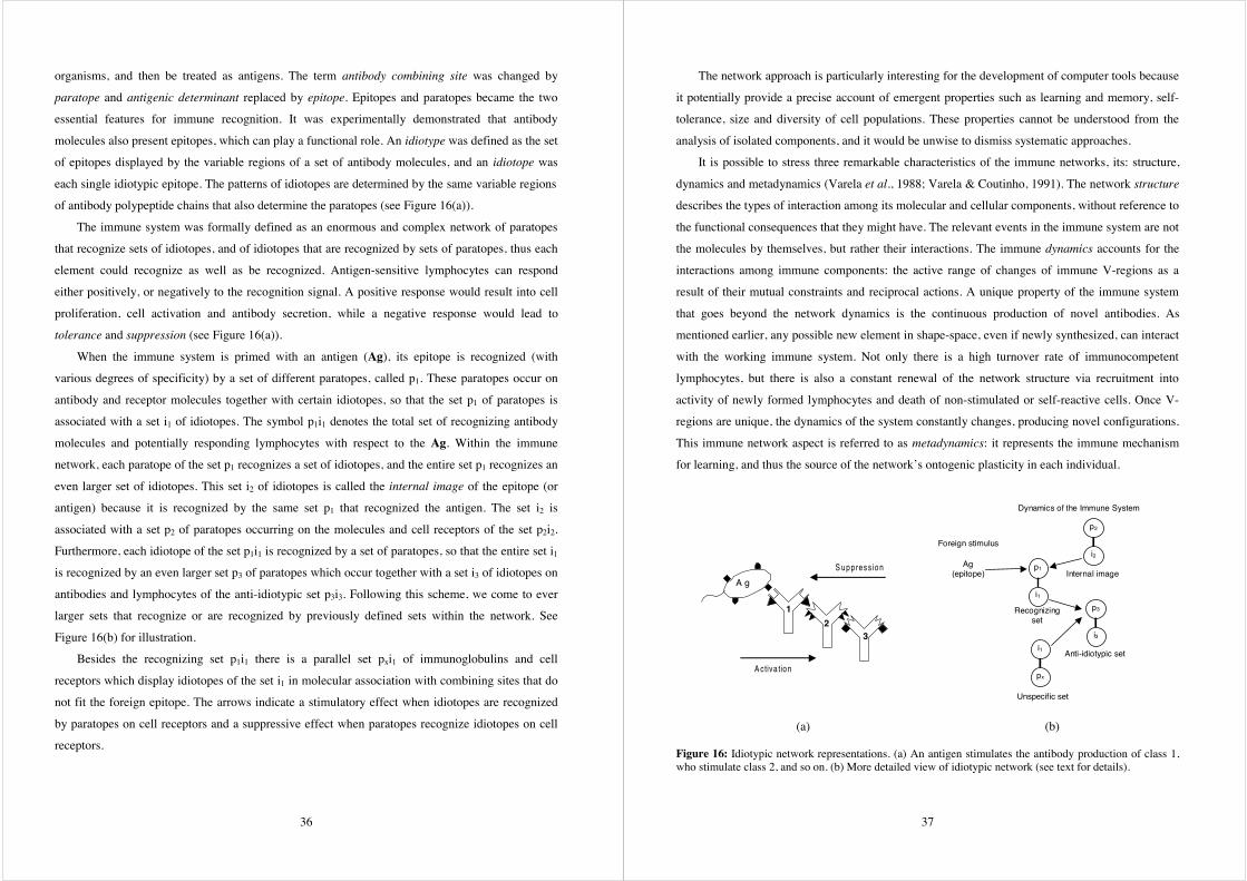
36
organisms, and then be treated as antigens. The term antibody combining site was changed by
paratope and antigenic determinant replaced by epitope. Epitopes and paratopes became the two
essential features for immune recognition. It was experimentally demonstrated that antibody
molecules also present epitopes, which can play a functional role. An idiotype was defined as the set
of epitopes displayed by the variable regions of a set of antibody molecules, and an idiotope was
each single idiotypic epitope. The patterns of idiotopes are determined by the same variable regions
of antibody polypeptide chains that also determine the paratopes (see Figure 16(a)).
The immune system was formally defined as an enormous and complex network of paratopes
that recognize sets of idiotopes, and of idiotopes that are recognized by sets of paratopes, thus each
element could recognize as well as be recognized. Antigen-sensitive lymphocytes can respond
either positively, or negatively to the recognition signal. A positive response would result into cell
proliferation, cell activation and antibody secretion, while a negative response would lead to
tolerance and suppression (see Figure 16(a)).
When the immune system is primed with an antigen (Ag), its epitope is recognized (with
various degrees of specificity) by a set of different paratopes, called p1. These paratopes occur on
antibody and receptor molecules together with certain idiotopes, so that the set p1 of paratopes is
associated with a set i1 of idiotopes. The symbol p1i1 denotes the total set of recognizing antibody
molecules and potentially responding lymphocytes with respect to the Ag. Within the immune
network, each paratope of the set p1 recognizes a set of idiotopes, and the entire set p1 recognizes an
even larger set of idiotopes. This set i2 of idiotopes is called the internal image of the epitope (or
antigen) because it is recognized by the same set p1 that recognized the antigen. The set i2 is
associated with a set p2 of paratopes occurring on the molecules and cell receptors of the set p2i2.
Furthermore, each idiotope of the set p1i1 is recognized by a set of paratopes, so that the entire set i1
is recognized by an even larger set p3 of paratopes which occur together with a set i3 of idiotopes on
antibodies and lymphocytes of the anti-idiotypic set p3i3. Following this scheme, we come to ever
larger sets that recognize or are recognized by previously defined sets within the network. See
Figure 16(b) for illustration.
Besides the recognizing set p1i1 there is a parallel set pxi1 of immunoglobulins and cell
receptors which display idiotopes of the set i1 in molecular association with combining sites that do
not fit the foreign epitope. The arrows indicate a stimulatory effect when idiotopes are recognized
by paratopes on cell receptors and a suppressive effect when paratopes recognize idiotopes on cell
receptors.
37
The network approach is particularly interesting for the development of computer tools because
it potentially provide a precise account of emergent properties such as learning and memory, self-
tolerance, size and diversity of cell populations. These properties cannot be understood from the
analysis of isolated components, and it would be unwise to dismiss systematic approaches.
It is possible to stress three remarkable characteristics of the immune networks, its: structure,
dynamics and metadynamics (Varela et al., 1988; Varela & Coutinho, 1991). The network structure
describes the types of interaction among its molecular and cellular components, without reference to
the functional consequences that they might have. The relevant events in the immune system are not
the molecules by themselves, but rather their interactions. The immune dynamics accounts for the
interactions among immune components: the active range of changes of immune V-regions as a
result of their mutual constraints and reciprocal actions. A unique property of the immune system
that goes beyond the network dynamics is the continuous production of novel antibodies. As
mentioned earlier, any possible new element in shape-space, even if newly synthesized, can interact
with the working immune system. Not only there is a high turnover rate of immunocompetent
lymphocytes, but there is also a constant renewal of the network structure via recruitment into
activity of newly formed lymphocytes and death of non-stimulated or self-reactive cells. Once V-
regions are unique, the dynamics of the system constantly changes, producing novel configurations.
This immune network aspect is referred to as metadynamics: it represents the immune mechanism
for learning, and thus the source of the network’s ontogenic plasticity in each individual.
12
3
A g
A ctiva tion
S up pres s io n p1
i1
p2
i2
i1
px
p3
i3
Ag(epitope)
Dynamics of the Immune System
Foreign stimulus
Internal image
Anti-idiotypic set
Recognizingset
Unspecific set
(a) (b)
Figure 16: Idiotypic network representations. (a) An antigen stimulates the antibody production of class 1,who stimulate class 2, and so on. (b) More detailed view of idiotypic network (see text for details).

38
As a summary, the central characteristic of the immune network theory is the definition of the
individual’s molecular identity, because natural tolerance is a global property that cannot be
reduced to the existence or activity of single clones. It emerges from a germ-line encoded network
organization expressed early in the development, followed by the ontogenic learning of the
molecular composition of the environment where the system develops, by metadynamic recruitment
of the respective clones. The network organization imposes a dynamic pattern for natural antibodies
that is distinct from the immune responses to external antigens. Actually, such dynamic patterns are
perfectly compatible with the maintenance of memory that is not localized in memory cells, but
distributed as a pattern.
9.1 Immune Network × Neural Networks
The nervous system is commonly decomposed into sensory and motor parts. An analogous
separation into recognition and effector functions can be made in the immune system, where
effector mechanisms lead to the elimination of the antigens. In neural systems, assimilation of
memories appears to be achieved by alteration of the strengths of connections between neurons,
rather than changes within the neurons themselves. Further, the brain allows memories to be
addressable by content, so that the frequent death of individual neurons does not drastically affect
the performance of the brain as a whole. The immune system possess a cross-reactive memory that
is observed when an individual develops a memory to one antigen and is challenged with a related,
but different one (Hoffmann, 1986; Ada & Nossal, 1987; Smith et al., 1997). The cross-reactive
memory, clonal expansion and programmed cell death rates allow the immune system to
dynamically allocate resources as needed in a distributed environment (Dasgupta, 1999).
Some important common features, as basic cognitive mechanisms (see Section 6.3), shared by the
neural networks and the immune system, are of great interest in this study, and can be described as
follows (Jerne, 1974; Hoffman, 1986; Vertosick & Kelly, 1989, 1991; Dasgupta, 1997, 1999):
• both systems consist of an enormous number and diversity of cells. In humans, the immune
system consists of roughly 1012 lymphocytes (B and T cells), and the central nervous system
consists of about 1010 neurons;
• the individual cells are highly specialized in their functions and present great diversity of
receptors;
• the immune system recognizes and responds to complementary shapes of a great variety of
large molecules. The nervous system recognizes and responds to different kinds of patterns,
like visual, auditory and sensory stimuli;
39
• the synaptic strengths between neurons can be excitatory (stimulating) or inhibitory
(depressing), giving rise to many different activity patterns. The inter-lymphocyte interactions
via cell-cell contact, or via chemical mediators have varying strengths which can be helping
or suppressing;
• both systems exhibit memory, early impressions leave a particularly deep and lasting imprint
into the network. Patterns of synaptic strengths constitute a memory that is auto-associative
and non-hereditary. Some activated lymphocytes become special memory cells that are
content-addressable, and non-hereditary;
• in the nervous system, a combination of global/local learning rules occurs, while changes in
lymphocyte concentration and constitution of receptors compose the mechanisms for learning
within the immune system; and
• definite recognition can be achieved with a threshold affinity. The immune and nervous
systems share this property.
9.1.1 Neural Network Approaches to the Immune System and Vice-Versa
Hoffman (1986) introduced a particular neural network model based on the analogy between
immune and neural networks. He presented a remarkable catalogue of similarities between the
immune system and the central nervous system, and stated that these similarities are strong at the
system level, but weak at the level of the components. His model of a neuron exhibits hysteresis,
and a network of N such neurons is modeled by an N-dimensional system of ordinary differential
equations, which exhibits almost 2N attractors.
Vertosick & Kelly (1989) suggested that the immune network theory would represent a role for
parallel distributed processing. In a later work (Vertosick & Kelly, 1991), they stated that the
immune system might represent an alternative system in which to search for neural network
architectures. They proposed that the network stores and retrieves large, complex antigenic patterns.
Their paper is concluded by remarking that the immune system is an ideal biological example of a
parallel distributed processing (PDP) network, with no need for symbolic logic, mathematical
operations or rule-based reasoning.
Abbattista et al. (1996) presented an associative memory model for storing and retrieving noisy
patterns based on the immune network. They tried to increase the memory capacity and retrieval
performance, of a variation of the discrete Hopfield network (Hopfield, 1984) by exploring the
meta-dynamical characteristics of the immune system.

40
10. An Evolutionary System
The clonal selection functioning of the immune system reveals it to be a remarkable microcosm of
Charles Darwin’s law of evolution (Perelson et al., 1978; Cziko, 1995; Adams, 1996), with the
three major principles of repertoire diversity, variation and natural selection, each playing an
essential role. Repertoire diversity is evident in that the immune system produces far more
antibodies than will be effectively used in binding with an antigen. In fact, it appears that the
majority of antibodies produced do not play any active role whatsoever in the immune response. As
previously discussed, natural variation is provided by the variable gene regions responsible for the
production of highly diverse population of antibodies, and selection occurs, such that only
antibodies able to successfully bind with an antigen will reproduce and maintained as memory cells.
The similarity between adaptive biological evolution and the production of antibodies is even
more striking when one considers that the two central processes involved in the production of
antibodies, genetic recombination and mutation, are the same ones responsible for the biological
evolution of sexually reproducing species. The recombination and editing of immunoglobulin genes
underlies the large diversity of the antibody population, and the mutation of these genes serves as a
fine-tuning mechanism (see Section 4). In sexually reproducing species, the same two processes are
involved in providing the variations on which natural selection can work to fit the organism to the
environment (Holland, 1995). Thus, cumulative blind variation and natural selection, which over
many millions of years resulted in the emergence of mammalian species, remain crucial in the day-
by-day ceaseless battle to survival of these species. It should also be noted that recombination of
immunoglobulin genes involved in the production of antibodies differs somewhat from the
recombination of parental genes in sexual reproduction. In the former, nucleotides can be inserted
and deleted at random from recombined immunoglobulin gene segments and the latter involves the
crossing-over of parental genetic material, generating an offspring that is a genetic mixture of the
chromosomes of its parents.
Whereas adaptive biological evolution proceeds by cumulative natural selection among
organisms, research on the immune system has now provided the first clear evidence that
ontogenetic adaptive change can be achieved by cumulative blind variation and selection within
organisms. The natural selection can be seen to act on the immune system at two levels. First, on
multiplying lymphocytes for selection of higher affinity clones for reaction with pathogenic
microbes. Second, on multiplying people for selection of the germ-line genes that are most able to
provide maximal defense against infectious diseases coupled with minimal risk of autoimmune
disease.
41
11. Immune Engineering Tools and Applications
In this section, we are going to present three algorithms, developed using ideas from immunology,
aiming at solving machine-learning tasks. We intend to study problems like search-space coverage,
knowledge acquisition, pattern recognition and classification, function approximation, multi-modal
optimization and parity problems of various sizes.
In Section 11.1, it is presented a Simulated Annealing approach to increase diversity (SAND)
in a binary model of the antibody repertoire. Its extension to real-valued shape-spaces is also
discussed. Section 11.2 introduces an Antibody Network (ABNET) that hybridize immunological
concepts with the neural network paradigm. The outcome is a boolean constructive neural network
model of cognition in the immune system, capable of performing pattern recognition and
classification with high levels of generalization. Finally, in Section 11.3, it is described an
implementation of the clonal selection algorithm, considering the affinity maturation of the
repertoire. It is shown that the proposed algorithm, called CSA for clonal selection algorithm,
performs learning and multi-modal optimization.
The performance of all the algorithms is illustrated through their application to engineering
tasks with various levels of complexity.
11.1 Diversity
The natural immune system is a complex pattern recognition device with the main goal of
protecting our body from malefic external invaders, called antigens. The primary elements are the
antibodies, which bind to antigens for their posterior destruction by other cells. The number of
antibodies contained in our immune system is known to be much inferior to the number of possible
antigens, making the diversity and individual binding capability the most important properties to be
exhibited by the antibody repertoire. In this paper, we present a simulated annealing approach that
aims at generating a dedicated pool of candidate solutions that best covers the search-space. The
strategy assumes no a priori knowledge about the problem and produces a fixed-size set of potential
candidates. The algorithm induces diversity in a population by maximizing an energy function that
takes into account the Hamming distance between binary strings. Our model compares favorably
with randomly generated antibody populations, and the results demonstrated its improved binding
characteristics without the use of a referential antigen population during the repertoire definition. Its
extension to Euclidean spaces and its potential to machine-learning applications are also discussed.

42
11.1.1 The Simulated Annealing Approach to Diversity (SAND)
In typical applications of genetic algorithms, the evolutionary strategy produces increasingly fit
organisms among an explosive number of candidates in highly uncertain environments. The
algorithm is used to evolve a population of potential candidate solutions, where a single member is
going to specify the best solution, i.e., a fitness peak. The selection and genetic operators
(crossover, mutation and inversion) used in the GAs guide the average population towards its fittest
member (Mitchel, 1998). In our application, we are searching for a cooperative population, which,
as an ensemble of individuals, is able to perform a specific computational task: maximizing the
coverage of the search-space, based on a fixed-size population. Under this point of view, there is no
single individual to be considered as the fittest one, but the whole population will represent the
solution, hence multiple fitness peaks will be desirable. This objective suggests that the standard
GA might not produce the desired result, and instead of developing a GA strategy capable of
maintaining the diversity of the population (Forrest et al., 1993; Matsui, 1999; Smith et al., 1993),
we chose to use a Simulated Annealing (SA) approach, which also has the advantage of being less
computationally intensive, in general.
Notice that the strategy we are proposing has the same essence as the Michigan approach
employed by the Classifier Systems (CS) introduced by Holland (1975). The Michigan approach
can be perceived as a computational model of cognition, where the knowledge of the entity is
expressed as a collection of rules that interacts with the environment and undergoes modifications.
Like in our Simulated Annealing method, the whole set of rules (i.e., population) represents a single
candidate solution.
The SA algorithm makes a connection between statistical mechanics and multivariate or
combinatorial optimization (Haykin, 1999; Kirkpatrick et al., 1987). The origin of the method is
associated with aggregate properties of a large numbers of atoms to be found in samples of liquids
or solid matters. The behavior of the system in thermal equilibrium, at a given temperature, can be
characterized experimentally by small fluctuations around the average behavior. Each atomic
position is weighted by a probability factor
)/exp()( TEEP Δ−=Δ , (6)
where E is the energy of the configuration, T the temperature and ΔE a small deviation in the energy
measured.
At each step of this algorithm, an atom is given a small random displacement and the resulting
change, ΔE, in the energy of the system is computed. If ΔE ≤ 0, the displacement is accepted, and
43
the configuration with the displaced atom is used as the starting point of the next step. The case
ΔE > 0 is treated probabilistically: the probability that the configuration is accepted is given by
Equation (6).
The temperature is simply a control parameter in the same unit as the cost (energy) function.
The simulated annealing process consists of first “melting” the system being optimized at a high
effective temperature, then lowering the temperature by slow stages until the system “freezes” and
no further change occurs. At each temperature, the simulation must proceed long enough for the
system to reach a steady state. Notice that, transitions out of a local optimum are always possible at
nonzero temperatures (steps of increasing temperature can also be incorporated). The sequence of
temperatures and the size of the ΔE variation attempted to reach equilibrium at each temperature are
considered an annealing schedule.
Now, we propose a cost (energy) function for our model, named SAND (simulated annealing to
diversity), that allows the detection of self-recognizing individuals (Equation (7)) and also the
maximization of the Hamming distance (HD) among them (Equation (8)). Let
⎩⎨⎧ ≠
=otherwise,0
,1),( ji xx
jiS , (7)
),(2),( 2 jiHDNl
jiF×
= , (8)
( )∑ ∑= +=
+×=N
i
N
jjiFjiSE
1 1),(),(
2100
. (9)
D(i,j) is a square, symmetric matrix responsible for the self/nonself discrimination, and xi, i = 1,...,
N, represents the members of the antibody population. It is composed of ones or zeros only, where a
1 indicates self-recognizing individuals and a 0 represents unique members (see Equation (7)).
Matrix F(i,j) is also a square, symmetric matrix that contains the Hamming Distance (HD) among
all individuals in the population (see Equation (8)). Equation (9) is the percentile energy of the
whole Ab repertoire, and is equal to 100% when there are no self-recognizing individuals in the
population and their distance is maximal.
Notice that, if the number of individuals in the population is less than the total number of
different individuals that can be generated for a string of length L (2L - for binary strings), then
different populations may give rise to the same maximal energy (100%) and the “optimal”
repertoire is not unique. This limited-size population may never reach the total coverage of the

44
search space, for ε = 0, but certainly it will reach some state close to the maximum possible
coverage, based on its restricted size and the pre-defined value of ε.
11.1.2 Related Works
Many authors have already addressed the problem of studying diversity and self/nonself
discrimination in the immune system under the machine-learning perspective. The algorithm
proposed can be seen as a model to increase diversity in a binary set of patterns or as a model to
perform self/nonself discrimination, where the self-recognizing members of the population are
avoided. In this work, we only explore the former idea, and the algorithm was studied as a tool for
generating populations with high levels of diversity. For good surveys on the self/nonself
discrimination issue (or negative selection) under the machine-learning context, refer to Dasgupta
(1999b) and Ishida (1996).
In Smith et al. (1993), the problem of using a genetic algorithm (GA) to search for a population
of cooperative structures was considered, where the GA had to discover a set of pattern matching
antibodies that effectively match a set of antigen patterns. Their strategy employed an immune
system model based on binary strings and demonstrated to perform multi-modal GA optimization
with various degrees of generalization. Using the same model, Forrest et al. (1993) studied the
pattern recognition processes and learning that takes place at both the individual and species level in
the immune system.
In Hightower et al. (1995), a binary model of the immune system was proposed to study the
effects of evolution on the genetic encoding used to represent antibody molecules. One feature of
the encoding used in this approach is that, unlike typical genetic algorithms, not all genes found in
the genotype are expressed in the phenotype. They studied the coverage of the antigens space and
their genetic organizations, concluding that the GA can optimize complex genetic information.
Oprea & Forrest (1998, 1999) used genetic algorithms to study the survival probability of an
individual with relation to the size of its germline-encoded antibody repertoire, in the context of a
shape-space model. As in all previous strategies, their antibody population was evolved based on
the recognition of a given antigen set. They concluded that for their Ag-Ab matching rules, there
was a scaling relation between the fitness and the size of the evolved library, which is only a shifted
variant of the scaling relation obtained with random libraries of same size. These works (Oprea &
Forrest, 1998-1999), like the one presented in Hightower et al. (1995), used libraries of genes, from
which gene fragments are orderly concatenated to lead to the formation of functional antibodies.
45
In all these models, the diversity of the antibody repertoire was a function of the intrinsic nature
of the antigen population to be recognized, i.e., an individual fitness was evaluated according to the
success of the antibody repertoire in recognizing randomly generated and selected antigens. Our
proposed strategy is not directly comparable to the previous ones, once we search for an antibody
population independently of any specific set of antigens. This method can be viewed as a blind
strategy, where no specific knowledge about the problem is assumed a priori, and the antibody
population is not developed based on a comparison between the response of some individuals of
this population and a desired response.
11.1.3 Strategy Evaluation
In order to evaluate the performance of the proposed method, we studied its ability to increase
diversity in randomly generated populations of various sizes and compared the binding affinity
(Ag−Ab) of the populations evolved (optimized) with that of populations uniformly generated. The
results achieved by the proposed algorithm and its potential applicability to solve machine-learning
tasks are discussed. In our implementation, both the temperature T and the disturbance introduced in
the energy of the system follow a geometric decreasing schedule, where the multiplying parameter
belongs to the interval (0.8, 0.99). The populations to be evolved by the SAND approach do not
take into account any antigen population, which are used only for evaluation.
11.1.3.1 Diversity
Table 3 presents a comparison of the energy (fitness) of the population (Equation (9)), taken over
twenty runs, for randomly generated populations (RP) and the ones evolved by the proposed
method. It can be seen that the SAND is able to maximize the energy of randomly generated
populations, i.e., it is able to maximize the search-space coverage, or population diversity.
From Table 3, we conclude that if we randomly generated an antigen population (Ag) with
strings of length L = 3, 4, 5, 6 or 7, the evolved populations of antibodies would be able to bind any
of these antigens for any size of the affinity threshold (ε), indicating a perfect binding Ag−Ab (see
Figure 17(a)). In this case, a value of ε > 1 implies that there will be cells in the intersection of the
sets defined by some antibodies, generating cross-reactive antibodies that can bind with both
antigens, initiating a cross-reactive response (see Figure 17(b) and the next section). If the antibody
repertoire (Ab) was generated randomly, it would be necessary an affinity threshold ε > 0 for some
antigens to be bound, meaning that the random population does not possess any possibility of
presenting a maximum shape-space coverage (see Figure 17(c)).

46
Table 3: Energy measure (fitness) of randomly generated populations (RP) versus fitness ofevolved populations (SAND). N is the size of the population and L the length of the bitstrings.The results are the maximum, minimum, mean and standard deviation of both algorithms takenover twenty runs.
RP (%) SAND (%)L 2L N Max Min Mean std Max Min Mean std3 8 8 81.25 50.00 68.12 9.06 100 100 100 04 16 16 78.12 62.50 69.06 4.76 100 100 100 05 32 32 73.44 62.50 68.28 3.61 100 100 100 06 64 64 73.44 64.06 69.45 2.91 100 100 100 07 128 128 71.48 66.80 68.32 1.46 100 100 100 08 256 128 71.68 66.21 69.30 1.62 100 100 100 09 512 256 68.18 63.48 65.38 1.26 100 100 100 0
ε = 1
ε = 1
(a) (b) (c)
Figure 17: Search-space coverage, (×) correspond to the antigens that represent the whole search-space, and(•) are the antibodies. (a) There are enough antibodies for covering all the universe of antigens. The SAevolved a population capable of maximum coverage of its space, avoiding self-recognizing states (ε < 1);there is a superposition among all the possible antigens and the evolved antibodies. (b) Beyond thesuperposition Ag−Ab, for ε > 1, intersections of the sets of cells stimulated by the antigen will occur. (c) Therandomly generated population may contain enough antibodies for covering the whole shape-space (N = 16),but there is a superposition of some of them (which is represented by the circles around the dots and crosses).
11.1.3.2 Cross-reactivity
For a given string length L, in order to measure the cross-reactivity (generalization capability, or
antigen coverage) of the evolved antibody repertoire, we generated the population of all possible
antigens. A number Nind of individuals were randomly chosen from this population for evaluation.
The results presented in Table 4 are the maximum, minimum, mean and standard deviation,
obtained over 10 runs, of the percentage of correctly recognized antigens.
To define the match score of a population, we adopted a fuzzy (non-linear) matching function
and a simple threshold function. In the threshold activation, a bond is established only when the
value of the match score is superior to L − ε (see Figure 14(a)). In the non-linear case a sigmoid
activation function was used, where ε relies on the inflexion point of the curve (see Figure 14(b)).
47
Figure 14(b) implies that a match score greater than 5 will produce a high binding value, while a
match score of 3 corresponds to a binding value of approximately zero. In the sigmoidal activation
case, binding values equal to, or greater than, 0.5 indicate that the molecules are successfully
recognized.
Table 4 compares the recognition percentage of the evolved population of antibodies with
relation to randomly generated populations. For the threshold binding activation, Equation (4) holds
and the boundary defined by the affinity threshold is a well-defined frontier. In the non-linear case,
this frontier is fuzzy, meaning that the coverage now is only approximate, but not equal to, Equation
(4). It can be seen that the evolved populations posses improved recognizing capabilities.
0 1 2 3 4 50
10
20
30
40
50
60
70
80
90
100
ε
Rec
ogni
tion
(%)
RP x SAND
60
65
70
75
80
85
90
95
100
3 4ε
Rec
ogni
tion
(%)
RP x SAND
(a) (b)
Figure 18: Trade-off between the recognition capability and the affinity threshold ε. The dashed linecorresponds to the proposed method and the solid line corresponds to randomly generated populations,L = 12, N = 100, Nind = 14. (a) ε ∈ [0, 5]. (b) Zoom in the circled region of (a), ε ∈ [3, 4].
Table 4: Recognition percentage, where L is the string length, N the Ab cardinality, C the coverage of eachantibody (for a threshold activation) and Nind is the number of individuals randomly taken from the Agpopulation. ε = 1 in all cases.
Threshold Activation Sigmoidal ActivationRP (%) SAND (%) RP (%) SAND (%)
L N C Nind Max Min Mean Std Max Min Mean Std Max Min Mean Std Max Min Mean std3 4 4 8 100 75.0 94.4 7.6 100 100 100 0 100 75.0 93.1 9.5 100 100 100 06 32 7 64 100 93.8 98.1 1.9 100 100 100 0 100 92.2 97.3 2.5 100 100 100 09 256 10 512 100 98.6 99.5 0.4 100 99.4 99.9 0.2 100 98.8 99.4 0.3 100 99.6 99.9 0.2

48
Figure 18 presents the scaling of the recognition capability with relation to the threshold affinity for
a randomly generated population (RP – solid line) and the evolved one (SAND – dashed line), for a
string of length l = 12. In this case, out of a universe of 212 = 4096 possible different molecules,
only 14 individuals compose the antibody population, which was tested against Nind = 100
independent individuals randomly taken from the whole pool of cells. The idea here is to test the
SAND capability to optimize very small populations, when compared to the universe of possible
individuals to be generated. This aspect of the SAND approach will become more evident when we
use it, in Section 11.1.5, to define the initial set of candidate solutions (population) for a genetic
search.
11.1.4 Extension to Euclidean Shape-Spaces
In order to apply the proposed method to real-valued spaces, a new energy function (see Equation
(9)) has to be defined. As we are dealing with real-valued vectors, instead of bitstrings, the
Euclidean shape-space might be taken as an alternative to the Hamming shape-space. Other real-
valued shape-spaces could also be adopted, like the Manhattan shape-space. The Euclidean and
Manhattan shape-spaces differ from the Hamming shape-space in that, instead of using a Hamming
distance as the measure of affinity between the molecules, they use the Euclidean and Manhattan
distances, respectively (see Equations (10) and (11)).
∑=
−=L
iii yxED
1
2)( , (10)
∑=
−=L
iii yxMD
1,
(11)
where xi and yi represent independent vectors of length L.
The new energy measure to be optimized can be simply defined as the sum of the Euclidean
distance among all vectors
∑ ∑= +=
=N
i
N
ijjiEDE
1 1),( (12)
where ED(i,j) is a square, symmetric matrix that contains the Euclidean distance (ED) among all
individuals in the population, according to Equation (10).
While dealing with the Hamming shape-space, the stopping criterion (convergence measure) of
the SA algorithm was directly established as E = 100%. In the Euclidean shape-space approach, the
49
energy measure E is not a percentile value, and another stopping criterion, which takes into account
the diversity among the vectors, has to be defined.
The approach to be proposed here, involves the analysis of directional data. Given the vectors
xi, i = 1,..., N, it is initially necessary to transform them into unit vectors, i.e., to normalize them,
resulting in a set Ii of N unit vectors of length L (Ii ∈ ℜL, i = 1,..., N). The average vector is
∑=
=N
iiN 1
1 II . (13)
Considering the Euclidean distance case (Equation (10)), a metric to determine the maximum
distance among a set of unit vectors can be simply given by
( ) 2/1 IITR = , (14)
where T represents the matrix transpose operation, and R corresponds to the distance of the average
vector from the origin of the coordinate system. Equation (14) represents the amplitude of the
resultant vector, but nothing can be inferred about the distance among the individual vectors, which
is measured via the Euclidean distance, as given by Equation (10).
The stopping criterion (SC) to be used is
)1(100 RSC −×= . (15)
Equation (15) is the percentile norm of the resultant vector R , and is equal to 100% when this norm
is zero. In practical terms, a value close to 100% for the stopping criterion (SC) is a reasonable
choice.
Like in the Hamming shape-space case, if the number of individuals in the population is less
than the total number of different individuals that can be generated for a vector of length L, then
different populations may give rise to the same maximal stopping criterion (100%) and the
“optimal” repertoire is not unique. Notice that, the normalization operation will only be necessary
for evaluating the quality of the solution, and the original vectors can be kept within any interval
during the iterative process.
Generating the most diverse population of antibodies in ℜL corresponds to producing a set of
directions which is mostly spread over the space. To illustrate the performance of the algorithm,
consider the case of generating a set of vectors in ℜ2 that best covers the search-space (ℜ2). Figure
19(a) and (b) depicts the evolved populations for N = 3 and N = 9, respectively. Notice that the
algorithm was capable of generating directions with maximal coverage of the ℜ2 search-space.
Similar results can be achieved for any value of N and L, where L represents the dimension of the
Euclidean space (ℜL).

50
-1 -0.8 -0.6 -0.4 -0.2 0 0.2 0.4 0.6 0.8 1
-1
-0.8
-0.6
-0.4
-0.2
0
0.2
0.4
0.6
0.8
1
x
yInitial unit directions
-1 -0.8 -0.6 -0.4 -0.2 0 0.2 0.4 0.6 0.8 1
-1
-0.8
-0.6
-0.4
-0.2
0
0.2
0.4
0.6
0.8
1
x
y
Initial unit directions
(a-1) (a-2)
-1 -0.8 -0.6 -0.4 -0.2 0 0.2 0.4 0.6 0.8 1
-1
-0.8
-0.6
-0.4
-0.2
0
0.2
0.4
0.6
0.8
1
x
y
Final unit directions
-1 -0.8 -0.6 -0.4 -0.2 0 0.2 0.4 0.6 0.8 1
-1
-0.8
-0.6
-0.4
-0.2
0
0.2
0.4
0.6
0.8
1
x
yFinal unit directions
(b-1) (b-2)
Figure 19: Generation of unit directions using the SA approach applied to Euclidean shape-spaces. Thedashed arrows indicate the initial set of vectors (a), and the solid arrows represent the optimized vectors (b).(a-1, b-1) Three vectors (N = 3). (a-2, b-2) Nine vectors (N = 9).
11.1.5 Machine-Learning Applications
Several machine-learning strategies are being used to solve problems like function approximation
and optimization. Among these, we can stress the application of genetic algorithms (Holland, 1975)
to search for the optimum (maximum or minimum) of a function, and the use of artificial neural
networks (ANN) (Rumelhart et al., 1986) to perform non-linear function approximation. Both
strategies (GA and ANN) require the definition of an initial set of candidate solutions (for the GA)
or initial weight vectors (in the ANN case). While employing these strategies, the initial sets are
usually defined randomly (or by using a uniform distribution). In order to illustrate the applicability
of the proposed method to other areas of research, we are going to use the SAND approach to
51
define an initial population set for a genetic search and to define the initial weight vectors for the
training of a multi-layer perceptron (MLP) neural network.
11.1.5.1 Genetic Search
Suppose we intend to maximize the following functions of a single variable: f1(x) = sin(x) + 1 and
f2(x) = sin(x) + 2 – 0⋅1 x. If we are going to employ an exploratory strategy, like a genetic algorithm,
or a gradient-based strategy, an set of initial conditions must be established. In these cases, the more
appropriate this initial set of conditions, the easier the search for the global optimum.
Figure 20 illustrates the above-mentioned functions (dashed curve) and two different sets of
initial conditions, where the crosses represent the optimized sets of initial conditions and the small
circles correspond to randomly generated initial conditions. Notice that the algorithm is capable of
diversifying the repertoire. Figure 20(a) illustrates 12 initial conditions for function f1 and Figure
20(b) depicts an initial condition composed of 10 values for function f2. The presence of very
similar individuals, composing a cluster, can be easily detected in the randomly specified sets (large
dashed circles). The SAND approach guides to a condition less susceptible to these situations. As
the set of individuals evolved by the proposed SAND algorithm are more spread over the universe
of the function, any local (or global) optimization strategy would reach a greater number of local
optima, increasing the likelihood of achieving the global optimum.
-10 -5 0 5 10
0
0.5
1
1.5
2
-10 -5 0 5 10
0
0.5
1
1.5
2
2.5
3
3.5
4
(a) (b)
Figure 20: The dashed line represents the mono-variable functions to be optimized, where the crossesrepresent the optimized populations (SAND) and the small circles correspond to randomly generatedpopulations (RP). (a) f1(x) = sin(x) + 1, population of size 12. (b) f2(x) = sin(x) + 2 – 0⋅1x, population of size10.

52
It is important to stress that the proposed algorithm also requires an initial set of conditions, but
independently of this set, it will reach a mostly diverse repertoire. If we consider the case where we
initially set the whole population with the same value, say x = −1, for example, the SAND approach
will still be able to diversify the population. Thus, no concern is needed about the start of the
iterative process employed by SAND method. In the examples depicted in Figure 20, the SAND
algorithm started from the initial conditions composed of the small circles and evolved them into
the crosses.
We employed the Hamming shape-space, with binary strings representing real values for the
variable x. The chosen bitstring length was l = 22, corresponding to a precision of six decimal
places. The variable x is defined over the range [−4π, 4π], and the mapping from a binary string
m = <ml,..., m2, m1> into a real number x is completed in two steps:
• convert the binary string m = <ml,..., m2, m1> from base 2 to base 10:
( ) ( ) '2.,,...,10
210212 xmmmm i
iiL ==>< ∑ =
• find the corresponding real value for x: 12
8 '4 22 −+−= xx , where −4π is the left boundary
of the domain, and 8π its length.
The affinity measures correspond to the evaluation of the functions f1,2(x) after decoding x, as
described above.
The SAND approach in the Hamming shape-space was used to define the initial population of a
standard genetic algorithm to maximize functions f1 and f2. Its performance was compared to that of
randomly generated populations. The parameters for the GA are: bi-classist selection (50% of the
best and 10% of the worst individuals are selected for reproduction), crossover probability pc = 0⋅6,
and mutation probability pm = 0⋅1. The stopping criteria were f1(x) = 2 and f2(x) = 4⋅1, respectively.
Table 5 shows the performance comparison for an initial population randomly generated (RP)
and an initial population evolved by the SAND method. The results presented were taken over ten
runs, where in each run, the population randomly generated was first applied to the GA and then
evolved by the SAND algorithm and re-applied to the GA. Different sizes (N) of the population
were tested. Figure 21 depicts the trade-off between the average number of generations for
convergence, for functions f1 and f2, for randomly generated populations (RP) and evolved
populations (SAND), as a function of N. These values were taken from column Mean of Table 5.
As discussed in Section 6.2, in most cases the SAND approach yielded very fast convergence rates
even when the population size is small, N < 10.
53
Table 5: Number of GA generations for convergence when the initial population is defined randomly (RP)or evolved by the SAND approach (results taken over ten runs).
f1 = sin(x) + 1 f2 = sin(x) + 2 – 0.1xRP SAND RP SAND
N Max Min Mean Std Max Min Mean Std Max Min Mean Std Max Min Mean std
4 27 1 11.3 7.7 25 1 9.8 8.5 335 17 109.3 120.8 90 2 39.7 29.1
6 22 1 11.9 8.9 9 1 3.6 2.7 141 5 49.3 42.6 105 1 27.7 32.9
8 14 1 3.3 3.9 6 1 2.1 2.1 171 5 42.3 61.6 94 1 26.2 31.4
10 14 1 5 4.74 10 1 3 1.1 35 1 15 13.6 21 3 9.8 5.5
20 3 1 1.4 0.7 1 1 1 0 43 1 9.9 12.6 19 1 6.7 5.7
30 2 1 1.1 0.3 1 1 1 0 54 1 11.6 16.8 10 1 3.8 2.9
0 5 10 15 20 25 300
2
4
6
8
10
12f1: RP (solid), SAND (dashed)
N
Gen
erat
ions
for c
onve
rgen
ce
0 5 10 15 20 25 300
20
40
60
80
100
120f2: RP (solid), SAND (dashed)
N
Gen
erat
ions
for c
onve
rgen
ce
(a) (b)Figure 21: Average, over ten runs, of the number of generations for the GA convergence for randomlygenerated populations (RP) and populations diversified by the SAND algorithm with relation to the size ofthe initial set. (a) Function f1. (a) Function f2.
11.1.5.2 Neural Network Initialization
As briefly discussed at the beggining of this section, the neural network training usually requires the
definition of an initial weight vector. It is required for networks like the multi-layer perceptron
(MLP) trained with the backpropagation algorithm (Rumelhart et al., 1986). This initial set of
weights, to be used in the MLP networks, has a strong influence in the learning speed and in the
quality of the solution obtained after convergence. The importance of a good choice for the initial
set of weights is stressed by Kolen and Pollak, 1990.
In this section, we are going to show empirically that the SAND approach is capable of
defining an initial set of weights for the MLP backpropagation training such that the convergence

54
speed of the algorithm is increased. To do so, we will use a variant of the backpropagation
algorithm, derived from the non-linear programming theory, called scaled conjugate gradient
(SCG) algorithm (Moller, 1993). This algorithm has the advantage that its rates of convergence are
higher than the standard backpropagation rates, but has the drawback that it converges to the closest
(from the initial condition) local optima. Hence, an appropriate definition of the initial set of
weights is crucial for its performance. Two neural network benchmark tasks and a real world
problem will be used for evaluation.
As the network weights are real-valued, the Euclidean shape-space must be employed. The
networks used posses a single hidden layer and are represented by net: [ni-nh-no], where ni is the
number of network input units, nh the number of hidden units and no the number of network outputs.
The sizes of the weight matrices are defined according to these parameters, i.e., w1 has dimension
ni × nh, and w2 has dimension nh × no. Let SSE be the sum of squared errors used as the stopping
criterion for the network training, and ns be the amount of available samples. The problems to be
tested are:
• XOR (exclusive-OR): ns = 4, net: [2-10-1], SSE = 0.1, w1 ∈ ℜ2×10, and w2 ∈ ℜ10×1;
• parity 4 problem: ns = 8, net: [4-15-1], SSE = 0.1, w1 ∈ ℜ4×15, and w2 ∈ ℜ15×1; and
• SOYA: a real world problem used by De Castro et al., 1998; ns = 116, net: [36-15-1], SSE =
0.1, w1 ∈ ℜ36×15, and w2 ∈ ℜ15×1.
For the matrices whose all dimensions are greater than 1, we can apply the SAND strategy to
increase the diversity of the initial weight vectors. In all these examples, the output weight vector,
w2, has dimension one and will be simply defined using a uniform distribution over the [−1, 1]
interval. Note that the problems are described in order of complexity. In the first case, XOR, the
SAND goal is to spread two vectors in ℜ10, and in the last case it has to increase the diversity of 36
vectors in ℜ15.
Table 6 shows the maximum, minimum, mean and standard deviations, over ten runs, for the
three problems tested. The SAND approach improved the convergence speed rates in all cases. The
results are compared to randomly initialized weight vectors. Like in the GA application, the weights
randomly initialized (RP) were optimized by the SAND and re-applied to the network training.
As in the GA applications, the SAND method demonstrated improved MLP rates of
convergence, when used to define the initial network weight vectors.
55
Table 6: MLP convergence speed (number of training epochs) for randomly initialized weight vectors (RP)and the optimized ones (SAND).
RP SAND
Problem Max Min Mean Std Max Min Mean Std
XOR 110 13 41.4 43.3 13 4 8.6 2.5
Parity 4 603 27 274.3 217.6 30 20 23.5 3.24
SOYA 244 196 218.9 16.4 185 125 147.2 17.5
11.1.6 Discussion
In this section we studied the advantages of diversifying a population through a simulated annealing
algorithm (SA). In order to do so, our model was inspired by the problem of pattern recognition (or
antigen coverage), intrinsic to the immune systems.
The developed algorithm constitutes a simple variant of the standard SA, but showed to be
useful in tackling the problem of pattern recognition in the immune system. Instead of evolving the
whole population in the search for one “optimal” individual, this search process is performed in a
competitive and cooperative manner, in the sense that new generation of individuals (a large
amount of individuals) are treated so that the more diverse individuals have a high probability of
being accepted into the pool of cells (a fixed-size small amount of individuals). At the end of the
learning process, the SA was able to find a solution that is mostly diverse and spread along the
solution space.
This method is particularly interesting if we are looking for a pool of candidate solutions (or
conditions) in an environment that contains restricted resources (candidates) and no knowledge
about the problem is assumed a priori. It might be used as a starting point for other optimization
strategies and will probably present poor results if the objective function to be optimized (energy or
fitness function) is well known and the search can be straightly directed toward this solution. In
addition, the results suggest that if we are searching for a single individual capable of best matching
a randomly chosen antigen, then our approach seems not to be competitive, once the cooperation-
based energy function will guide all members of the population to evolve together, not privileging
any of them in particular.
Our strategy is directly applicable to the problem of maximal coverage of the search-space and
self-recognition (redundancy avoidance) of generic Hamming-spaces by fixed-size populations.
Although it was introduced assuming a Hamming shape-space, the method was further extended to
deal with Euclidean shape-spaces and its potential applicability to machine-learning tasks was
discussed.

56
11.2 The Antibody Network (ABNET)
As discussed in Section 7, the human capability of solving problems like pattern recognition and
classification are usually addressed to the brain. Nevertheless, the immune system is capable of
recognizing and responding to micro-cells and molecules (like viruses, bacteria, funguses, etc.) that
can not be perceived by our sensory mechanisms that send stimuli to the brain. This way, it
performs an accessory role for nervous cognition. A great advantage of the immune system over the
nervous system, is the existence of several well-established theories that reasonably explain
immune functions, allowing us to develop more accurate models. In this work we show that some
immune theories can be successfully applied in the development of neural network architectures. A
novel neural network is presented, with the main features of competitive learning, automatic
generation of the network structure and binary representation of the connection strengths (weights).
The proposed network was applied to two simple real-world problems and a binary character
recognition task. The results show that the developed network, called ABNET, is a promising tool
for solving problems that are inherently binary and also, that the immune system provides a new
paradigm in which to search for neural architectures.
Some important cognitive aspects of the immune response to an antigenic stimulus can be
listed: recognition of the antigen, maturation of the response (learning) and memory acquisition and
maintenance. Artificial connectionist devices have been successfully and widely used to model
systems with similar capabilities (Rumelhart et al., 1986; Hopfield, 1982). In this work, we propose
a constructive algorithm to generate a Boolean competitive neural network model, based upon
properties of the clonal selection paradigm of the immune system. The antibody repertoire is
modeled using a connectionist approach, with an antibody network being generated, where the
connection strengths of the network represent the molecules, and the recognition is performed in a
systemic level, rather than by single individuals. Several characteristics of the immune response are
taken into account, such as: the clonal expansion of the most stimulated cells, the programmed cell
death (apoptosis) of non-stimulated cells and the affinity maturation of the repertoire.
A splitting algorithm embodies the cloning of the most stimulated cells, while the cell death is
performed by a pruning mechanism. A hypermutation strategy is used to increase the affinity of the
network cells during the construction process and to fine-tune the grown network. In terms of
codification, a binary model of the ABNET, based on the shape-space formalism (Perelson & Oster,
1979), is used to build a minimal antibody repertoire capable of binding any antigen represented in
this same shape-space. The antigen receptor and the B cell receptor are assumed to interact to the
extent that their shapes are complementary (DeBoer et al., 1992). This is modeled by assuming that
57
the cells interact maximally whenever their coordinates in the shape-space have a maximum
distance, and that the strength of interaction falls off for less complementary shapes in a manner
described by a threshold function of the Hamming distance between the pair of interacting shapes.
The development of the immune repertoire during neonatal life involves a strong selection
process among different antibodies. The natural immune system is genetically capable of producing
a much more diverse set of lymphocyte receptors than are expressed in the actual repertoire
(Coutinho et al., 1984; DeBoer & Perelson, 1991). Hence, in this work, the artificial networks we
model do not have a predetermined size or topology. Rather, the pre-existing antigens will represent
the guiding force responsible for selecting the available antibodies for expansion. These expanded
cells (clone) can either be incorporated into the network or be discarded. Antibodies (Ab) are
removed from the network (network pruning) if they fail to expand, which means that they do not
match any of the elements contained in the antigen (Ag) population. The network grows if it still
did not reach the minimal size necessary to bind every antigen available in the Ag population, given
an affinity threshold (ε). In some cases, e.g. when there is redundant Ag, the network may not even
reach the minimal pre-defined architecture, remaining still smaller. Hence, this process is composed
of a growing phase and a pruning phase.
As the network evolves, it develops a number of self-regulatory features. Most importantly, the
network attains a specific equilibrium size and generates a characteristic amount of antibodies.
Once the ABNET reaches an equilibrium size, the new candidate antibodies must compete with the
established ones to enter the repertoire.
Under the point of view of an immunologist, the task performed by the algorithm to be
proposed is equivalent to generating the antibody repertoire of minimal size for recognizing any
antigen within a given population. Under the machine learning perspective, the algorithm presents a
constructive, unsupervised learning strategy for a Boolean competitive network. Moreover, the
model can be used to study cross-reactive responses, which is a process that involves the concept of
generalization capability, much studied in the neural network community.
11.2.1 Describing the Network
Primarily, it will be assumed the existence of an antigen (Ag) population to be recognized by the
antibody repertoire, i.e., a problem to be solved. We assume that the antibody repertoire contains a
single individual at the beginning of the learning process, so that the repertoire will have to be
constructed while submitted to the Ag population (nevertheless, the network can start with any pre-
determined size). For the sake of simplicity, the cells will be uniquely represented by their receptors

58
(Ab), which are assumed to be of same length as the antigens. The antibody repertoire will be
modeled as a Boolean competitive network, called “antibody network” (ABNET).
The main features of the antibody network to be developed, are as follows:
• growing architecture, based on the clonal selection principle;
• network pruning, representing the death of non-stimulated cells (apoptosis);
• boolean connection strengths; and
• competitive network, with unsupervised learning based on a mutation mechanism.
In our cognitive paradigm (antigen recognition, learning and memory), it is desired to build an
antibody network for maximal coverage of the antigen space. In order to do so, we will take the
shape-space notation and the notation used to describe some classes of neural network models (see
next Section for a description of related neural networks).
Under the neural network paradigm, the patterns we want to recognize are usually called
learning samples (or training patterns) and the units composing the network are called neurons (see
Sections 2 and 3). In the shape-space domain, the input patterns are the antigens (Ag), and the
neurons are simply called cells. An antibody k (Abk) will be represented by the weight vector wk
connecting the network inputs to a single output unit k. All these units are linear processing
elements, i.e., they compute the weighted sum of their inputs (a linear combination between the
input and weight vectors). One distinct characteristic of this network is that its weights are binary
(Hamming shape-space), i.e., 0’s or 1’s, instead of real-valued, like in the majority types of neural
networks.
Ab population
Ab re-selection
Clone Death
Affinity maturation
Most stimulated cell Non-stimulated cell
Ab selection
Antigenic stimuli
Neurons (k)
Competition
Split Prune
Weightupdate
Winner Inactive neuron
Input patterns
(a) (b)Figure 22: Main steps of the algorithm. (a) Immune system perspective. (b) Neural network paradigm.
59
The initial architecture might be composed of a single output unit whose weights represent a
hypothetical single antibody in the antibody network. A concentration level τj, determines the
concentration of antigens for each antibody ( j ) in the network, and together with the antibody with
highest affinity to the antigen, select an individual for cloning.
The competitive learning algorithm (Haykin, 1999) had to be adapted to support some features
of our modeled ABNET. Primarily, as both the input patterns Ag and the weight vectors w are
binary, the distance between Ag and w (Ab) is given by the Hamming distance (affinity, see Figure
14 – Section 6.2).
The cell k of the antibody repertoire, with the highest affinity to a given antigen Ag, is
considered to be the one whose weight vector Abk presents the largest Hamming distance to this
antigen:
kkk AbAg −= maxarg . (16)
The construction of the model requires one last parameter to be defined, va, which is a labeling
vector of the molecules with highest affinity, e.g. if Ab7 is the highest affinity antibody for Ag9,
then v9 = 7.
The main loop of the competitive algorithm can be summarized as follows:
1. Choose an antigen (input pattern) Aga according to its probability density distribution
P(Ag).
2. Determine the highest affinity cell Abk, according to Equation (16).
3. Update the weight vector wk of the most stimulated cell (see Section Weights Updating).
4. Increment the concentration level τj for the selected cell (j = k).
5. Attribute va = k.
Figure 22 presents a diagram with the main steps of the developed algorithm, where Figure 22(a)
stresses the algorithm under the immune system perspective and Figure 22(b) represents the neural
network paradigm. The processes of affinity maturation in the immune system and of weights
updating in the neural network are equivalent, both aim at increasing the quality of the response to
the pattern to be recognized. The cloning of the most stimulated cell (splitting), together with the
death of non-stimulated cells (pruning), are always verified and performed after a certain number of
adaptation steps (cell generations). Our goal is to reach a minimal antibody network, as a function
of P(Ag) and the affinity threshold ε. This is achieved when every unit has the same probability of
being the highest affinity cell for the current input vector and for a given ε. As we do not know
P(Ag) explicitly, we use the concentration level (τj) to estimate its value.

60
11.2.1.1 Network Growing
This process mimics the selection and reproduction of the most stimulated cell, according to the
clonal selection principle. In our model, the most stimulated cell to be selected is the one with
highest affinity with the antigen and that is confronted with the highest concentration of antigens.
As we want to generate a parsimonious ABNET, each selected cell will suffer a single mitosis, and
the two generated cells will turn into memory cells after their maturation.
The growing procedure we adopted is based upon two parameters: the concentration level τj
and the affinity threshold ε. All cells whose τj > 1 are potential candidates to be split, and cell s
which is subject to the highest concentration of antigens is chosen as the single candidate. This
process is described in Equation (17), and if no cell j satisfies this criterion, then the network
architecture remains frozen.
}1|{ where, maxarg >==∈
jjjOj
Os AbAb . (17)
If the affinity of cell s, with relation to the antigen that best matches it, is larger than the affinity
threshold ε, then the candidate cell s is the most stimulated cell and will be cloned; else the network
architecture remains with the same size. The more antigens a cell has an affinity with, the more
stimulation it will receive from the environment. The network promotes the reinforcement of the
units that are very stimulated, favoring the cloning of these cells.
The weights of the new clone are the exact complement of the worst matching antigen of cell s.
This is not in perfectly accordance with the original clonal selection principle, but it generates an
antibody network such that it perfectly matches all the given antigens, and the described growing
procedure guides the network straight to this final configuration, reducing the number of iteration
steps required for convergence.
On the other hand, if the network was used to automatically generate clusters, the new clone
should have been be inserted as a neighbor of s. This idea mimics the neighborhood preservation
addressed in the Kohonen self-organizing networks (Kohonen, 1982), contrasting with our
approach.
As an illustrative example, suppose there is an antigen population to be recognized composed
of the following three individuals: Ag1=[0,0,0], Ag2=[1,1,1], Ag3=[1,0,0]. The initial network
configuration contains a single antibody molecule represented by the weight vector w=[1,1,1]. As
there is a single antibody in the network, the labeling parameters vi, i = 1,...,3, contain the same
value 1, i.e., cell 1 recognizes all antigens (see Figure 23(a)).
61
Ag3
1
0
0
Ag1
0
0
0
Ag2
1
1
1
1
1
1
1
v1=1 v2=1 v3=1
τj =3
Ag3
1
0
0
Ag1
0
0
0
Ag2
1
1
1
11
1
1 2
00
0
(a) (b)
Figure 23: (a) Assignment of the parameters τj and va, where τj defines the concentration level of eachantibody, and va labels the cells with the highest affinity with each given antigen. Agi, i = 1,...,3, are theantigens (input patterns); w1 = [1,1,1] represents Ab1. (b) Cloning and defining the weights of the new cell,w2 = [0,0,0].
The antigen with highest affinity (most complementary) with this antibody is Ag1, and the lowest
affinity antigen is Ag2 (see Equation (16)). This cell will be selected for cloning and its progeny will
have weights complementary to its worst matching antigen, Ag2, w=[0,0,0]. Figure 23(b) depicts
the generation of the new cell and the definition of its weights. Notice that this procedure
guarantees a broader and faster coverage of the antigen space.
11.2.1.2 Network Pruning
Kepler & Perelson (1993a,b) suggested that a short burst of somatic hypermutation, followed by a
“breathing interval” to allow for selection and clonal expansion, might form the basis of the
maturation process. The selection mechanism may provide a means by which the regulation of the
hypermutation process is made dependent on receptor affinity. Cells with low affinity receptors may
be further mutated and, as a rule, die through apoptosis. In cells with high-affinity antibody
receptors, however, hypermutation may be turned off (see Section 4.2).
The pruning policy (mimicking apoptosis) is as follows: if a cell p has its concentration level
equals to zero (τp = 0) longer than a specified length of time, then it can be deleted from the
network. As proposed by De Castro & Von Zuben (1999) in another context, after pruning a
competitive network, the value of the learning rate (that corresponds, in this case, to the
hypermutation rate to be described in the next section) might be restored to its initial value. This
restarting procedure is supposed to allow the pruned network to properly redefine its connection
scheme. Restoring and controlling the hypermutation rate may simulate the burst and breathing
suggested by Kepler & Perelson (1993a,b).
To illustrate the network pruning, consider the same previous example: an antigen population
composed of Ag1=[0,0,0], Ag2=[1,1,1] and Ag3=[1,0,0]. Assume, either that a network with three
units (w1=[1,1,1], w2=[0,0,0], w3=[1,0,0]) has been constructed, according to Figure 24(a). In this

62
case, the vectors v = [1,2,1], and τ = [2,1,0], indicating that cell three (3) will be selected for
pruning, once it is not stimulated by any antigen (notice that this procedure is usually applied after a
certain number of iterations). After pruning unit 3, the remaining network is depicted in Figure
24(b). This pruning policy aims at keeping the specificity of the antibodies, due to the fact that only
those antibodies that do not recognize any antigen, after a certain period of time, will be excluded
from the network.
Figure 25 depicts a hypothetical growing network. The black dots represent the remaining cells
(after growth and pruning), the circles represent the cloned cells and the dashed circle represent the
cell that was pruned back the network during the learning/growing process. The input units and its
connections are only depicted in the initial (a) and final (c) networks.
Ag3
1
0
0
Ag1
0
0
0
Ag2
1
1
1
1
2
3
w1=[1,1,1], τ1=2
w2=[0,0,0], τ2=1
w3=[1,0,0], τ3=0v1=1 v2=2 v3=1
Ag3
1
0
0
Ag1
0
0
0
Ag2
1
1
1
1
2
w1=[1,1,1]
w2=[0,0,0]
(a) (b)
Figure 24: Pruning of non-stimulated cells. (a) Cell three (3) is not being stimulated by any antigen (τ3 = 0)for a period of time longer than a pre-defined number of cell generations. Agi, i = 1,...,3, are the antigens(input patterns); w1 = [1,1,1] represents Ab1, w2 = [0,0,0] represents Ab2 and w3 = [0,0,0] corresponds toAb3, ε = 1. (b) Resultant network, with only two cells.
1 1
2
3
4
5
6
7
8
9
10
11
8
9
10
11
7
(a) (b) (c)Figure 25: Constructing the network. Squares: input units; black circles: remaining cells; circles: clonedcells; dashed circle: pruned cell. (a) The initial network. (b) Network growing and pruning (inputconnections are omitted). (c) Resultant network architecture with its labeled cells.
63
11.2.1.3 Weights Updating
Another important aspect of the adaptive immune response is the affinity maturation of the antibody
repertoire through a hypermutation mechanism. Antibodies present in a memory response have, on
average, a higher affinity to the antigens than those of the early primary responses (Berek &
Ziegner, 1993). This is achieved mainly through a mutation mechanism with high rates, followed by
a strong selective strategy.
The weight updating process used in our antibody network is similar to a multi-point mutation
(Holland, 1995; Mitchel, 1998) with variable rates. The hypermutation rate α determines how many
points of the bitstring will be mutated. The only states allowed are 0 or 1, for binary strings, and the
non-complementary positions are candidates to be changed, resulting in a directed search through
the shape-space. The weights updating is a guided search, such that the weights become a more
perfect complement of the antigens (see Figure 26), inducing a controlled affinity maturation of the
antibody combining sites. If the weight vector is the exact complement of the antigen (Ag), then no
updating takes place.
Berek and Ziegner (1993) also suggested that the mutation rate is proportional to the antibody
affinity with the antigen, implying that higher affinity antibodies suffer lower mutation rates. In the
binary network, the mutation rate α ∈ +}0{Z , where +
}0{Z is the set of nonnegative integers, possesses
an integer decreasing scheme, and after a pre-specified number of iterations, the α value is
decreased by one, until it reaches α = 0, what represents no updating at all. This is usually achieved
when the antibody molecule has maximal affinity with the antigen it recognizes.
1 0 0 0 1 0 1 1
0 0 1 1 1 1 1 0
0 1 1 1 1 1 1 0
Ag
Abk (Affinity: 5)
Ag
Abk (Affinity: 6)
1 0 0 0 1 0 1 1
Updating (α = 1)
1 0 0 0 1 0 1 1
0 0 1 1 1 1 1 0
0 1 1 1 0 1 1 0
Ag
Abk (Affinity: 5)
Ag
Abk (Affinity: 7)
1 0 0 0 1 0 1 1
Updating (α = 2)
(a) (b)Figure 26: Updating procedure for antigens of length l = 8, where the mutation positions are chosenrandomly among the non-complementary ones. (a) α = 1. (b) α = 2.
11.2.2 Related Networks: Competitive, Hamming, Boolean and Others
In this section, we intend to briefly discuss several neural network architectures that are somehow
related to the presented algorithm. The main characteristics of the proposed network are the use of a

64
binary (Boolean) weight vector and a competitive growing learning scheme based on the Hamming
distance between the weight set and the input patterns. These characteristics make the algorithm
very suitable for digital (VLSI) implementation, and, then a few comments about hardware neural
implementation will also be presented.
In competitive learning, the output units of a neural network compete among themselves to
become active (fired), and only a single unit is active for each input vector (pattern). There are two
basic elements in a competitive learning: a set of neurons with the same input-output behavior,
except for their weight vectors, and a mechanism for competition among neurons (Haykin, 1999).
The one that wins the competition is called a winner takes all neuron. The individual neurons learn
to specialize on ensembles of similar patterns. By doing so, they become feature detectors for
different classes of input signals. The Kohonen Self-Organizing Map (SOM) describes a map ΨX→O
which projects data points x ∈ ℜd, to a neuron k in some output space O (Kohonen, 1982). The
mapping prescription is competitive, and follows the winner takes all rule, i.e. x is mapped onto that
neuron k ∈ O whose weight vector wk ∈ ℜd is closest to x,
kkOX k wxx −=Ψ → minarg: . (18)
The adaptation procedure of the SOM, is like the adaptation in the competitive learning
mentioned above, with the difference that not only the connections of the winner neuron are
updated, but the connections of Nc neighbors are also shifted toward x. Other important
characteristics of the SOM are the application of decaying adaptation parameters, like the learning
rate (α) and Nc, and the possibility of implementing growing (Fritzke, 1994; Cho, 1997; Bauer &
Villmann, 1997) and pruning (Castro & Von Zuben, 1999) procedures in order to properly define
the network architecture. The competitive scheme used by the ABNET, can be seen as the dual of
the competitive scheme applied to the ordinary competitive networks (compare Equations (2) and
(4)). In addition, the ABNET is also capable of controlling its size (through growing and pruning
procedures) like some classes of self-organizing networks, and it also possesses a variable learning
rate, as in the SOM case. The pruning self-organizing map (PSOM) proposed by Castro & Von
Zuben (1999), suggests that all those units that do not classify ξ% of the data, are not relevant and
shall be pruned. They also suggested that, after pruning, restoring parameters α and Nc may lead to
improved input-output mappings. Parameter ξ is called pruning threshold.
The Hamming network (Lippman, 1987) is similar to the proposed method in the sense that
both networks are competitive and perform the Hamming distance between a set of connection
strengths and the input patterns, but differ completely with relation to the learning algorithm. In the
65
Hamming network, the architecture is two-layered and of fixed-size, the weights are assigned
(instead of trained) according to the data set and the units of the lower layer posses biases. On the
other hand, the ABNET is constructed during learning, has a single layer of connection strengths
and does not have biases to the output units, resulting in a more parsimonious architecture. Both
networks are designed to deal effectively with binary data sets and are very suitable for hardware
implementation, mainly due to their intrinsic binary operations. Examples of hardware
implementation of the Hamming networks can be found in the works of Robinson et al. (1992),
Çilingiroglu (1993) and Schimid et al. (1998).
The class of networks where the input and output vectors are strings of binary bits (0 or 1) are
usually called Boolean or binary networks. In this group of networks, the representation obtained by
the training algorithm becomes a logic circuit implemented by threshold gates working as hidden
and output units. Examples of algorithms derived from original principles of Boolean algebra can
be found in Biswas & Kumar (1990) and Gray & Michel (1992). In this case, the learning scheme is
completely different from the ABNET and takes into account Boolean algebra operations, instead of
biological inspiration. A general neural unit (GNU) has been introduced as a building block for
neural systems (Aleksander & Morton, 1991; Browne & Aleksander, 1996). The GNU is capable of
retrieving learned prototype images at internal connections when stimulated by distorted versions of
the prototypes at the external terminals. The network connections can only assume the values 0,1 or
u, for an undetermined connection.
Within the class of networks designed to deal effectively with binary input data, we can also
consider one version of the original Hopfield network (Hopfield, 1982-1984), which can be used as
a content addressable memory. This network contains N threshold logic units, and binary inputs are
used for learning. The output of each unit is fed back to all other nodes via weights. As in the
Hamming networks case, the weights of the Hopfield network are assigned, instead of trained like
in the ABNET. The "trained" network is iterated until it converges to a steady-state, when a new
pattern is presented. The output, after convergence, must be compared with the original input
patterns in order to determine if it exactly matches an exemplar. Sometimes this network might
converge to spurious states, i.e., states different from the stored fundamental memories. The weights
of the discrete Hopfield network can be assigned using the Moore Penrose Pseudo-Inverse method
(Denker, 1986), according to the following expression:
w = P(P×P+)-1PT , (19)
where w is the weight matrix, P the data matrix, -1 the inverse operator and T the transpose operator.

66
Implementing a real-valued neural network on a digital or mixed analog and digital chip yields
the quantization of the synaptic weights dynamics (Thiran et al., 1994). The use of a network that is
inherently Boolean, in the sense that its weights and updating learning rule deal with binary values,
makes the proposed algorithm a strong candidate for hardware (or digital) implementation without
concerning with the quantization effects on the weights and network parameters. Several works
addressing the problem of implementing neural networks on dedicated hardware can be listed
(Hochet et al., 1991; Gioiello et al., 1991; IEEE, 1992; Ienne & Kuhn, 1995).
Although the ABNET is not directly comparable to any of the networks presented, some of
them were implemented for comparison, and the results will be discussed in the next section.
11.2.3 Performance Evaluation
The ABNET performance was verified against three different problems and compared with the
results presented by other network architectures. The examples are of different nature, and each of
them aim at testing a particular capability of the network under evaluation. Let N be the number of
training samples of size ni, and no the number of outputs. To reduce the deviation in the
comparisons, all the results presented are the average over ten runs. The tasks can be described as
follows.
11.2.3.1 Fitting Contact Lenses (LENSES)
This pattern recognition (classification) problem was used by Witten & MacDonald (1988) to study
knowledge acquisition. This dataset is available for download in the repository of machine learning
databases of the University of California (URL 1). Nine rules cover the training set and the
examples are complete and noise free, but constitute a high simplification of the problem. There are
24 instances (N = 24), mapped into three classes, and the number of attributes (inputs) is 4 (ni = 4).
This is a simple classification problem and we intend to test the network capability to learn the
input samples. It is important to notice that this task is not binary, requiring a binary modeling of
the dataset for the application of the ABNET. The original inputs assume only the values 1, 2 or 3
that will be represented by 1: [1 1 1]; 2: [0 1 0] and 3: [0 0 1], implying a total number of 12 bits to
represent the 4 inputs. The numbers 1, 2 and 3 could have been modeled using only two bits,
instead of three, as was done, but this would result in numbers with different Hamming distances
(HD) to the others, e.g., if 1: [1 1]; 2: [0 1] and 3: [0 0], the HD between numbers 1 and 2 is one,
but between numbers 1 and 3 is two. The chosen modeling keeps a symmetric HD among the three
values.
67
Table 7: Results produced by the application of four methods to the problem LENSES. PCC is the percentileof correct classification, no is the network number of outputs, ε is the affinity threshold and ξ is the pruningthreshold. The results are the average and standard deviation taken over ten runs. In the CL and SOM cases,we arbitrarily chose different number of outputs to present, though other values were tested.
CL SOM ABNET PSOMno PCC (%) no PCC (%) ε no PCC (%) ξ no PCC (%)24 92.50 ± 1.75 24 97.08 ± 3.43 0 24 ± 0.00 100 ± 0.00 0.001 13.7 ± 1.30 95.00 ± 4.3019 92.50 ± 1.75 19 96.67 ± 2.64 1 24 ± 0.00 100 ± 0.00 0.005 12.7 ± 1.06 92.08 ± 4.9914 92.92 ± 2.01 14 96.25 ± 3.07 2 21.9 ± 0.88 97.08 ± 3.43 0.01 13.2 ± 1.81 92.92 ± 4.839 92.09 ± 1.32 9 92.09 ± 1.32 3 21 ± 1.41 95.83 ± 3.93 0.05 8 ± 0.00 91.67 ± 0.00
LENSES 4 75.00 ± 4.81 4 77.50 ± 8.83 4 18.2 ± 1.23 93.75 ± 4.05 0.1 8 ± 0.00 91.67 ± 0.00
The ABNET was compared with the competitive learning approach (CL), the standard one-
dimensional self-organizing map (SOM) and the pruning self-organizing map (PSOM) (see Section
5 for a brief description and references). The CL network possesses a fixed number of outputs no,
pre-specified before training, and its average percentile of correct classification (PCC) is presented,
along with its standard deviation taken over ten runs. The same measures were taken for the
standard SOM algorithm. The results for the ABNET takes into account the affinity threshold (ε)
and a variable number of outputs. The PSOM algorithm requires the specification of the pruning
threshold (ξ) and the final number of outputs is also variable. As the CL, SOM and PSOM are real-
valued networks, the inputs were taken as originally presented, but normalized over the interval
[-1, 1].
Table 7 depicts the results of the application of the CL, SOM, ABNET and PSOM algorithms
to the problem LENSES. It can be observed that, due to the use of a binary representation to model
a real-valued problem, the ABNET reached final architectures that are the least parsimonious ones,
when compared with the PSOM algorithm, for example. On the other hand, the ABNET
demonstrated to be very powerful for knowledge acquisition, being able to classify the patterns with
100% accuracy, when an affinity threshold of 0 or 1 is used. In these cases, the networks evolved
contain antibodies (weight vectors) highly specific for the antigen population.
11.2.3.2 Binary Character Recognition (CHAR)
This problem aims at evaluating the noise tolerance and generalization capability of the ABNET,
when presented to binary input patterns. In this case, the ABNET was compared with the discrete
Hopfield network described in the previous section. The storage scheme for the Hopfield net, was
the Moore Penrose Pseudo-Inverse.

68
Figure 27: Ten 7×5 artificial binary characters to test the network noise tolerance.
The input patterns used to test the network noise tolerance were artificially generated and are
depicted in Figure 27. Random noise was inserted into the learning samples by simply reverting a
bit 0 into a 1, or vice-versa. We tested four different noise levels: 5.7% corresponding to the shift of
2 bits, 11.4% corresponding to a 4 bits shift, 20% corresponding to the shift of 7 bits and, finally,
40% corresponding to the shift of 14 bits. The ABNET was tested for different values of the affinity
threshold (ε = 0, 1, 2, 3, 4 and 5) and a correct classification is assumed when the network maps the
corrupted pattern (pattern with noise) into the same node as the original pattern (pattern without
noise). In the Hopfield network case, a correct classification is considered, when the Hamming
distance between the restored pattern and the stored one is smaller than a value δ, where (δ = 0, 1, 2,
3, 4 and 5).
Figure 28 depicts the results for both strategies. It can be seen, from this figure, that if it is
required a perfect recovering by the Hopfield network, i.e. HD = 0 between the restored pattern and
the corrupted one, then its performance shows a strong degradation with the noise level. The
ABNET demonstrated to be less sensitive to the noise level than the Hopfield network. It is
important to remark that parameters δ and ε are not directly comparable. While δ represents the
accuracy of the steady-state achieved by the Hopfield network at the end of the iterative process
(measuring the existence of spurious states), ε indicates the affinity threshold necessary for the
ABNET learning. However, for practical purposes, the role of both parameters is rather equivalent.
In order to evaluate the generalization capability of the proposed network, it was used a
different set of characters (see Figure 29(a) for illustration). This dataset is composed of twenty-
nine 20×20 characters, where six of them are different patterns for the letter A, and the others
represent other letters of the alphabet. The idea here is to train the network with this dataset and to
see if it can recognize the characters presented in Figure 29(b), which are different patterns for the
letter A, assumed to be samples of the same class as the learned A characters.
69
54
32
10
0.40.3
0.20.1
00
20
40
60
80
100
δ
Noise Tolerance - Hopfield
Noise level
Cla
ssifi
catio
n (%
)
01
23
45
0.40.3
0.20.1
020
40
60
80
100
ε
Noise Tolerance - ABNET
Noise level
Cla
ssifi
catio
n (%
)
(a) (b)
Figure 28: Noise tolerance of the Hopfield and ABNET. δ is the allowed HD between the pattern recoveredby the Hopfield network (a) and the stored pattern, and ε is the affinity threshold of the ABNET (b).
(a)
(b)Figure 29: Characters to test the generalization capability. (a) Samples of the alphabet, with six differentletters A. (b) Independent test set.
Figure 30 shows the patterns recovered by the Hopfield network and the pattern association
performed by the ABNET. It can be seen that the Hopfield network could not recover one character,
ending in a spurious state. The ABNET grouped together different kinds of A into two groups,
leading to a correct classification.

70
Hopfield ABNET (ε ≥ 55)
Test
Retrieved patterns
Test
Associated patterns
Test
Associated patterns
(a) (b)
Figure 30: Results obtained for the Hopfield and ABNET algorithms. (a) The Hopfield network could notassociate one of the independent patterns with its stored fundamental memories. (b) For ε ≥ 55, the ABNETassociated and grouped together two sets of the independent A patterns.
Figure 31 shows how the ABNET generalization capability varies with relation to the parameter ε.
This picture shows that the classification for the training patterns is degraded with ε, but the
generalization capability for the A class does not suffer too much degradation, keeping itself around
92%. This phenomena leads to the conclusion that the ABNET is maintaining, at least, one class for
the A patterns, and is mixing up the other characters (see Figure 30). This is justifiable, once the A
class is predominant in the given dataset.
0 10 20 30 40 50 60 70 80 90 100
40
50
60
70
80
90
100
ε
Correct C lassificationTest: Train:
Figure 31: Generalization capability versus affinity threshold (ε) (Train and Test patterns presented inFigure 29).
71
11.2.3.3 Major Logic Decision (MLD)2
In order to evaluate the network behavior in real world applications, we applied the proposed
algorithm to the major logic decision (MLD) problem. It will initially be made a brief description of
the MLD problem and then the ABNET performance will be compared to that of other neural
architectures.
Problem Description
A possible application of the digital communication service is the investigation of spread spectrum
modulation using the FH-FSK (Frequency Hopping – Frequency Shift Keying) non-coherent
detector, as proposed by the Bell laboratories (Goodman et al., 1980; Einarson, 1980).
The block diagram for the FH-CDMA multi-level transmitter is shown in Figure 32(a). All
binary operations considered are taken over the Galois field GF(Q). The resulting codeword sent
through the channel by a sequence of L FSK signals is given by
xay += (20)
where x represents a Q-ary message generated by the m-th user, and a its address, both of length L
(L < Q). a is added componentwise to the user message.
These FSK sequences can be represented as inputs to a matrix of Q rows and L columns
(Einarson, 1980). The duration of each of these sequences is called the chip time. As an example,
consider a system with Q = 7 and L = 5 (see Figure 32(b)).
Message Address Codeword
Message FSK Modulator
Address
x
a
y
(a)
(b)
Figure 32: (a) Block diagram for the FH-CDMA multi-level transmitter. (b) Example with Q = 7 and L = 5:)1 ,1 ,1 ,1 ,1(=x , )4 ,1 ,6 ,0 ,3(=a and ).5 ,2 ,0 ,1 ,4(=y
2 This section was performed in collaboration with Getúlio A. de Deus Jr., from the Department of Communication(DECOM/FEE/Unicamp).

72
The transmission matrix corresponds to the message of the user )1 ,1 ,1 ,1 ,1(=x added to its address
),4 ,1 ,6 ,0 ,3(=a resulting in a codeword ).5 ,2 ,0 ,1 ,4(=y Notice that, in this case, the codeword address
was cyclically moved of one step (module 7 addition). The FSK sequence can be affected by the
sequences of other users and, also, by fading and noise. In this work, we did not considered the
fading and noise effects, hence only other users could interfere in the data transmission and
reception.
The receiver is composed of a frequency-dehopper, which extracts the address of the received
FSK sequence, and Q energy detectors. During the L chip intervals, the outputs of the detectors are
compared with a threshold and a decision is made about whether the corresponding frequency is
present or not. A maximum likelihood majority rule receiver, for the message m, is given by the
following rule
1 , ,2 1, 0,),|(max −= Qmyrp mm(21)
where r is the receiver matrix, my is one of the possible matrixes (transmitted by the user m) that is
being decoded, and p(⋅ | ⋅) is the conditional probability.
Thus, a maximum likelihood receiver that minimizes the error probability for messages with
equal a priori probabilities, can be implemented by a majority rule receiver that selects the message
y as the transmitted codeword (matrix) with more entries in the received matrix.
Neural Receivers for the MLD Problem
Several neural network approaches have been proposed and tested to tackle the major logic decision
problem. In De Deus Jr. et al. (1999a) a neural network architecture and learning algorithm,
specially designed to solve the major logic decision problem, was introduced. This network, called
NTNET (non-trainable neural network), is composed of two modules, where the first module
performs the sum of the rows of the matrix, and the second module is competitive, being
responsible for the determination of the decodified message. The NTNET allows the design of a
major logic receiver with a set of Q threshold-logic neurons. Other neural network architectures
were also used for comparison (De Deus Jr. et al., 1999a,b): the multi-layer perceptron (MLP),
trained with the standard backpropagation algorithm, and the pruning self-organizing map (PSOM),
as described in Section 5. Notice that, these latter networks have real-valued weight vectors, while
the ABNET and the NTNET posses binary connection strengths. To apply the MLP network to this
task, we simply adopted one output to each training pattern and performed the supervised learning.
73
10
Q
...10
10
1 2 L 1 2 L 1 2 L
Figure 33: Matrix representation of the training patterns for the MLD problem.
In order to compare the behavior of the above-mentioned networks, consider a system with Q = 7
and L = 3. In this case, solving the major logic decision problem implies in designing a receptor
with a performance, in terms of word error probability, as given in Figure 34. The word error
probability describes the probability of correct decoding the sent message.
1 2 3 4 5 6 710-2
10-1
100
Number of Users
Wor
d Er
ror P
roba
bility
Figure 34: Major logic decision performance for a system with Q = 7 and L = 3. The word error probabilityrepresents the probability of correctly decoding the sent messages, and is equal to 0 for a number of usersless than 4.
Table 8: Network complexity to solve the MLD problem. MLP is the multi-layer perceptron, NTNET thenon-trainable network, PSOM the pruning SOM and ABNET the proposed algorithm. The final number ofconnections presented is taken after the elimination of the zero-valued weights.
NeuralNetwork
Number ofConnections
ArchitectureComplexity
BinaryRepresentation
MLP 181 High NoNTNET 21 Low YesPSOM 21 Low No
ABNET 21 Low Yes

74
All networks were capable of solving the problem (i.e., achieving the desired word error
probability). Nevertheless, their training algorithms are completely different, making their
performance comparison, in terms of number of iterations for convergence and accuracy, difficult.
Hence the networks were compared with relation to their architecture complexity, i.e., the number
of connection strengths (weights and biases) at the end of the training process. The smallest MLP
network capable of solving the problem contained 181 connections, with 21 inputs, 6 hidden units
and 7 outputs. The NTNET required only 21 connections. If we discard the zero-valued connections
of the ABNET, its resulting architecture also contained 21 connections. The PSOM algorithm
resulted in a network with 147 real-valued connections (21×7). However, the PSOM weights’ can
be quantized (decoded) to assume the values of 0 or 1 and, if we discard these zero-valued
connections, the remaining network will also have only 21 connection strengths. Table 8
summarizes the performance comparison of the algorithms with relation to their architecture
complexity. This table also indicates that the intrinsic binary representation of the weights, make the
NTNET and the ABNET particularly suitable for solving the MLD problem.
11.2.4 Discussion
For the MLD problem, the main advantage of the ABNET over the other networks tested, is that it
represents a general architecture, with a learning strategy of Boolean kind, which can be applied to
different settings. The other network that demonstrated to be competitive (NTNET) was specially
designed to solve the MLD problem, and shall be adapted before being applied to other tasks.
In the example described in Section 11.2.3.1, the proposed network was capable of performing
knowledge acquisition with high rates of pattern recognition. It could also be noticed that, as
proposed in the theory, for very small values of ε (e.g. ε = 0 or ε = 1), the resultant ABNET is
highly specific for the antigenic patterns and many units are inserted in order to perfectly represent
the antigens. The more generalist the network is required to be (ε ≥ 2), the fewer units are added,
and the more parsimonious the solution. The user shall define the desired trade off between the
quality of recognition and the complexity of the resultant net.
The ABNET has some advantages over the Hopfield network, as originally proposed (Hopfield,
1984), to solve binary character recognition problems. It implements a kind of optimum minimum
error classifier when bit errors are randomly and independently assigned to the input patterns, and
thus the performance of the Hopfield net must either be worse than or equivalent to that of the
ABNET in such situations. The ABNET also required many fewer connections than the Hopfield
net for the problem tested: e.g., to test the generalization capability, the Hopfield network required a
75
weight matrix of size 400×400 (160,000 connections) while the ABNET required a 400×29 (11,600
connections) weight matrix, for ε = 0. The ABNET can also be modified to be a minimum error
classifier when the input patterns are bipolar, and errors are generated by reversing input elements
from +1 to −1 and from −1 to +1 asymmetrically with different probabilities. Finally, the ABNET
does not suffer from spurious states that can produce no-match results.
While exposing the backpropagation algorithm, Rumelhart et al. (1986) discussed seven
problems, among which we can name, for convenience, six of them: XOR, parity, encoding,
symmetry, addition and negation. In all these examples, the learning network can be
straightforwardly classified as Boolean, where the information from the outside world are encoded
into binary bits by the input units of the learning network. Due to its pattern of connection and
learning scheme, the ABNET is capable of solving problems like these in a straightforward way,
while some real-valued networks, like the perceptron trained via the backpropagation algorithm
might have difficulties and, also, demand a great computational effort for convergence. In addition,
the ABNET hardware implementation is more straightforward than in the ordinary networks case
and it is not subject to the quantization effects, once its weights and learning algorithm are of
Boolean kind.
11.2.5 Concluding Remarks
The complexity of the immune system is sometimes compared to that of the brain, however the
human has much more knowledge about the immune system than it has about the nervous behavior.
Most of the neural network models developed in the literature, are based upon observations and
abstractions of many neural activities, like pattern classification (perceptron), vision (Grossberg and
ART networks), associative memory (Hopfield net), etc. In this work, we pointed out many existing
similarities and differences between the nervous and immune systems. One of the most important
roles of immunity is its capability to recognize patterns that can not be perceived by the nervous
system, like viruses, bacteria and microbes, i.e. micro-invaders, called antigens. This way, the
immune function might complement neural perception, acting as a cognitive device.
The mechanisms by which the immune system recognizes and responds to an antigenic pattern
are believed to be well understood and were discussed in this paper. A mathematical formalism,
named shape-space, was used to quantify the interactions between the immune molecules and the
external invaders. In this work, we showed that these immune mechanisms are very appealing from
the computational perspective and the immune cognition might not only complement nervous
cognition, but also lead to the development of new neural network algorithmic models.

76
As a novel neural network model, the ABNET has the following features: competitive learning,
automatic generation (growing and pruning) of the network structure and binary representation of
the connection strengths (weights).
In order to properly evaluate the proposed ABNET, it was applied to a simple real-world binary
problem from the telecommunications field, a binary character recognition task and a non-Boolean
classification problem. The results demonstrated that the ABNET is a promising tool for application
in real-world and benchmark binary tasks, and its hardware implementation is straightforward, not
presenting the undesired quantization effects of some real-valued networks. Although the ABNET
can be classified as a Boolean network, its applicability to real-valued problems was also discussed
and illustrated.
Under the point of view of an immunologist, the task performed by the proposed algorithm is
equivalent to generating an antibody repertoire of minimal size, modeled as a network, to recognize
any antigen within a given population. Under the machine-learning perspective, the algorithm
represents a growing Boolean competitive network capable of solving complex machine-learning
problems, like knowledge acquisition, pattern recognition and classification.
The constructive characteristic of the proposed algorithm enables it to detect redundant patterns
and, in these cases, even though more units are allowed to be inserted into the network, it will not
happen. The redundant patterns will be recognized by the same unit, which represents a specific
class of patterns. This building strategy yields parsimonious network architectures, adaptable
according to the learning task under study.
11.3 An Implementation of the Clonal Selection Algorithm
The clonal selection principle is used by the immune system to describe the basic features of an
immune response to an antigenic stimulus. It establishes the idea that only those cells that recognize
the antigens proliferate, thus being selected against those which do not. The selected cells are
subject to an affinity maturation process, which improves their affinity to the selective antigens (see
Section 4). In this section, we propose a computational implementation of the clonal selection
algorithm, which takes into account the affinity maturation of the immune response. The algorithm
is shown to be capable of solving complex machine-learning tasks, like pattern recognition and
multi-modal optimization.
77
11.3.1 Model Description
In Section 4, we discussed the clonal selection principle and the affinity maturation process, which
will be used as the fundamental basis for the development of the clonal selection algorithm (CSA).
The main immune aspects taken into account were:
• maintenance of the memory cells functionally disconnected from the repertoire;
• selection and cloning of the most stimulated individuals;
• death of non-stimulated cells;
• affinity maturation and re-selection of the higher affinity clones;
• generation and maintenance of diversity; and
• hypermutation proportional to the cell affinity.
The algorithm works as follows (see Figure 35):
(1) Generate a set (P) of candidate solutions, composed of the subset of memory cells (M)
added to the remaining (Pr) population (P = Pr + M);
(2) Determine the n best individuals Pn of the population P, based on an affinity measure;
(3) Clone (reproduce) these n best individuals of the population, giving rise to a temporary
population of clones (C). The clone size is an increasing function of the affinity measure of
the antigen;
(4) Submit the population of clones to a hypermutation scheme, where the hypermutation is
proportional to the affinity of the antibody. A maturated antibody population is generated
(C*);
(5) Re-select the improved individuals from C* to compose the memory set. Some members of
the P set can be replaced by other improved members of C*;
(6) Replace d low affinity antibodies of the population, maintaining its diversity.
For each problem to be presented, the coding and affinity measure adopted will be discussed
separately.
Steps 2 and 3 are crucial in this algorithm. If we choose n = N in Step 2, i.e. the number of
highest affinity individuals equals the number of candidates, each member of the population will
constitute a potential candidate solution locally, implying a local exploitation of the shape-space,
characterizing a greedy search. In addition, if all the individuals are accounted locally, their clones
(Step 3) will have the same size. In all the example applications, steps 2 and 3 were taken as
discussed in this paragraph.

78
Maturate
Pr
M
Select
Clone
Pn
C
C*
(1)
(2)
(3)
(4)
(5)
Re-select
Nd
(6)
Figure 35: Block diagram of the algorithm implemented.
11.3.2 Examples of Applications
First, we are going to apply the algorithm to binary character recognition and demonstrate its
potentiality to perform learning and memory acquisition. Then, it will be applied to a multi-modal
optimization task and the well-known travelling salesman problem (TSP).
11.3.2.1 Learning and Memory Acquisition
The learning and memory acquisition of the CSA was verified through its application to a binary
character recognition problem. Our goal was to demonstrate that a cumulative blind variation
together with selection could produce individuals with increasing affinities (maturation of the
immune response). In this case, we assumed that the antigen population was represented by a set of
eight binary characters (N = 8) to be learned. Each character is represented by a bitstring (Hamming
shape-space, studied in Section 6.2) of length L = 120. Any arbitrary population size greater than N
(number of samples) would suffice to produce a single representation for each member of the
antigen population. This way, an antibody repertoire composed of 10 individuals, from which 8 of
them constitute the memory set, was taken. The original characters are depicted in Figure 36(h).
Figure 36(a) illustrates the initial memory set, and Figures 36(b) to 36(h) represent the maturation
of the memory set (immune response) through cell generations. The affinity measure takes into
account the Hamming distance between antigens and antibodies, according to Equation (3).
79
(a)
(b)
(c)
(d)
(e)
(f)
(g)
(h)
Figure 36: Application of the CSA to the binary character recognition problem. (a) Initial patterns to belearned. Memory set after 20 cell generations (b), 50 cell generations (c), 75 cell generations (d), 100 cellgenerations (e), 150 cell generations (f), and 200 cell generations (g). (h) Learned memory cells after 250generations (corresponding to the learning samples - antigens).
11.3.2.2 Multi-Modal Optimization
The clonal selection algorithm reproduces those individuals with higher affinities and selects their
improved maturated progenies. This strategy suggests that the algorithm performs a greedy search,
where single members will be locally optimized (exploitation of the surrounding space), and the
newcomers yield a broader exploration of the search-space. This characteristic makes the CSA very
suitable for solving multi-modal optimization tasks and, as an illustration, consider the case of
maximizing the function f(x,y) = x.sen(4πx)−y.sen(4πy+π)+1, depicted in Figure 37(a), in the
compact region [−1,2] × [−1,2] Notice that this function is composed of many local optima and a
single global optimum at f(1.63,1.63) = 4.25. Figure 37(b) represents a hypothetical set of 200
individuals randomly distributed over the search-space.
We employed the Hamming shape-space, with binary strings representing real values for the
variables x and y. The chosen bitstring length was L = 22, corresponding to a precision of six

80
decimal places. The variables x and y are defined over the range [−1, 2], and the mapping from a
binary string m = <mL,..., m2, m1> into a real number x or y is completed in two steps:
• convert the binary string m = <mL,..., m2, m1> from base 2 to base 10:
( ) ( ) '2.,,...,10
210212 xmmmm i
iiL ==>< ∑ =
• find the corresponding real value for x: 12
3 '1 22 −+−= xx , where −1 is the left boundary of
the domain, and 3 its length.
The affinity measure corresponds to the evaluation of the function f(x,y) after decoding x and y, as
described above.
(a) (b)
Figure 37: Function f(x,y) = x.sen(4πx)−y.sen(4πy+π)+1 to be optimized by the CSA and standard GA (a).Two hundred individuals (stars) uniformly distributed over the function (b).
(a) (b)
Figure 38: Function x.sen(4πx)−y.sen(4πy+π)+1 optimized (100 generations) by the GA (a) and CSA (b).
81
0 20 40 60 80 100 120 140 160 180 2000.5
1.0
1.5
2.0
2.5
3.0
3.5
4.0
4.5f(x,y) evolution - Average
Generation
f (x,y
)
GA
CSA
0 20 40 60 80 100 120 140 160 180 2002.5
3.0
3.5
4.0
4.5f(x,y) evolution - Best
Generation
GA
CSA
f (x,y
)
(a) (b)Figure 39: Evolutionary behavior of the decoded average value of f(x,y) (a) and the maximum value (b), forthe genetic and clonal selection algorithms.
Figure 38(a) and (b) presents the evolved populations, after 100 generations, by the standard genetic
algorithm (see Section 10.3.3 for a brief description of the standard genetic algorithm – GA) and the
clonal selection algorithm (CSA), respectively. Notice that the genetic algorithm guided the whole
population towards the global optimum of the function, while the CSA generated a diverse set of
local optima, including the global optimum.
Figure 39(a) compares the decoded average value of the function f(x,y), for the whole
population, evolved by the GA and the CSA algorithms. Figure 39(b) depicts the best individuals
(candidates with higher values for f(x,y)) of the populations for each algorithm. The GA approach
presented a greater average value, indicating a less diverse set of individuals. Both strategies
successfully determined the global optimum.
11.3.2.3 Solving the Travelling Salesman Problem
Simply stated, the travelling salesman must visit every city in his territory exactly once and then
return to the starting city. The question is: given the cost of travel between all cities, which is the
tour with smallest cost? For sake of simplicity, the reader must consider as cost, basically the length
of the itinerary traveled by the salesman.
The travelling salesman problem (TSP) is a kind of combinatorial optimization and arises in
numerous applications, from VLSI circuit design, to fast food delivery. In this case, the use of an
Integer shape-space might be appropriate, where integer-valued vectors, composed of permutations

82
of L, represent the possible tours. Each component of the integer vector indexes a city. The total
length of each tour gives the affinity measure of the population.
In Figure 40, we present the trade-off between the speed of the repertoire maturation with
relation to the clone size, for the TSP problem. The algorithm was allowed to run 20 generations,
with a population of size N = 10. The graph presents the maximum, minimum and mean values,
taken over ten runs. We can notice that, the larger the clone size, i.e., the size of the intermediate
population (C), the faster the reach of local optima.
Figure 41 presents how the immune algorithm evolves the best solution for a population of 300
individuals, with a rate of 20% of newcomers. In this case, low affinity individuals are allowed to
enter the repertoire after each 20 generations. This scheduling is supposed to leave a breathing
space to allow for the achievement of local optima, followed by the replacement of the poorer ones.
1 10 100 10000.5
0.6
0.7
0.8
0.9
1.0
1.1
1.2
1.3
1.4
1.5x 10
Clone size
Affin
ity
5
Figure 40: Trade-off between the speed of the maturation of the population with relation to the clone size,for the travelling salesman problem. Maximum, minimum and mean values taken over ten runs.
83
8 22
7
1
6
23
19
2421
2825
14
15
10
9
13
274
1112
3017
3
2 18
26
2029
16
5
TSP - 10 gen
19
21
12
411
27 30
26
24
29
28
20510
22
257
18
14
2
3
15
6
916
18
13
17
23
TSP - 50 gen
(a) (b)
2
14
81
5
7
22
25 28
29
2420
21
19
16
23
27 3017
1112
6
9
10 18
26
13
4
3
15
TSP - 100 gen
105
7
18
14
2
15
3
1323
27 3017
411
12
6
916
1926
24
29
2825
22
20
2118
TSP - 200 gen
(c) (d)
7
18
14
2
15
3
411
1213
17
23
27 30
2619
21
20
22
25 28
29
24
18
166
9
105
TSP - 250 gen
7
18
14
2
15
3
411
1213
17
23
27 30
2619
2124
29
2825
22
20
18
166
9
105
TSP - 300 gen
(e) (f)
Figure 41: Evolution of the clonal selection algorithm when applied to the TSP problem. Length of the tours(in u.d.m. – unit of distance measure): (a) 107932, (b) 75627, (c) 60913, (d) 54540, (e) 49433 and (f) 48872.

84
11.3.3 Genetic Algorithms × the Clonal Selection Algorithm
The Genetic Algorithms (GAs) constitute stochastic evolutionary techniques whose search methods
model some natural phenomena: genetic inheritance and Darwinian strife for survival. GAs perform
a search through a space of potential solutions, which are distinguished by the definition of an
evaluation (fitness) function, which plays the role of an environment feedback.
A genetic algorithm (or any evolutionary program) for a particular problem, must have the
following five components (Michalewicz, 1996):
• a genetic representation for potential candidate solutions;
• a way to create an initial population of potential solutions;
• an evaluation (fitness) function;
• genetic operators that alter the composition of an offspring;
• values for the various parameters used by the algorithm: population sizes, genetic
operators probabilities, etc.
Figure 42 depicts the block diagram for the standard genetic algorithm.
While the GA uses a vocabulary borrowed from natural genetics and is inspired in the
Darwinian evolution, the clonal selection algorithm (CSA) makes use of the shape-space formalism,
along with immunological terminology to describe Ag-Ab interactions and cellular evolution.
The CSA performs its search, through the mechanisms of somatic mutation and receptor
editing, balancing the exploitation of the best solutions with the exploration of the search-space.
Essentially, its encoding scheme is not different from that of genetic algorithms.
P
Select
Recombination
PI
Figure 42: Block diagram for the standard genetic algorithm (GA), where PI is the intermediate population.
85
11.3.4 Discussion
In this section we proposed a general purpose clonal selection algorithm inspired in the clonal
selection principle and affinity maturation of the immune responses. The algorithm was verified to
be capable of performing learning and maintenance of high quality memory and, also, it was
capable of solving complex problems, like multi-modal and combinatorial optimization.
By analyzing the proposed algorithm, called CSA (Figure 35), with the standard genetic
algorithm (GA) depicted in Figure 42, and the results presented, we can notice that the CSA
maintains a diverse set of local optimal solutions, while the GA tends to polarize the whole
population of individuals towards the best one. This occurs mainly due to the selection and
reproduction schemes adopted by the CSA and described in steps 2 and 3 of the proposed
algorithm. Essentially, their coding schemes and evaluation functions are not different, but their
evolutionary search differs from the viewpoint of inspiration, vocabulary and fundamentals.
However, we do not advocate that the CSA performs better than the GA in any application, instead
we demonstrate that it is also composed of a biologically inspired algorithm, which performs
learning and multi-modal search along the space. Like the GA, the clonal selection algorithm is
highly parallel.
12. Concluding Remarks and Future Directions
This technical report started with an instructive introduction to the immune system, followed by the
development of several engineering tools capable of solving complex problems in many areas of
research, like computation, mathematics, engineering and others. We strongly expect that this text
reinforces the importance of studying and using biological systems, in particular the immune
system, as powerful sources of inspiration for the development of alternative solutions to problems
that still can not be resolved by conventional engineering techniques.
The immune engineering was introduced as a new field of research that uses ideas gleaned from
immunology in order to generate dedicated solutions based solely upon the representation of the
problems. A set of potential candidate solutions can be defined, together with a function to measure
their affinity to the environment. The immune engineering might embody all immunologically
inspired strategies, including hybrid immune systems, artificial immune systems and their
applications, immunogenetic approaches, and others. In addition, the shape-space formalism was
proved to present a reasonable representation (vocabulary) for the development of immune
engineering tools.

86
It was demonstrated, through the development of several algorithms, that with simple systemic
views of the immune system, we can manage to engineer different computational techniques. The
applications used as illustration, focused on the generation of diversity, pattern recognition and
classification, function approximation, multi-modal and combinatorial optimization. However, other
types of examples could have been used to test the proposed algorithms, like control, system-
identification, computer security, sensor-based diagnosis, scheduling, fault detection, data analysis,
etc.
A technical report containing the review of the most striking achievements in the field of
immune engineering will also be available for download from the authors’ home page
(ftp://ftp.dca.fee.unicamp.br/pub/docs/vonzuben/lnunes/immunesystems). This report will bring an
extended list of references and brief descriptions models to be considered.
Although a few isolated attempts to establish a formal and general Artificial Immune System
have already been made, it is still one open question for artificial intelligence researchers.
AcknowledgementsLeandro Nunes de Castro would like to thank FAPESP (Proc. n. 98/11333-9) for the financial
support. Fernando Von Zuben would like to thank FAPESP (Proc. n. 98/09939-6) and CNPq (Proc.
n. 300910/96-7) for their financial support.
87
References
[1] Abbattista, F., G. Di Gioia, G. Di Santo & A. M. Farinelli (1996), “An Associative Memory Basedon the Immune Networks”, 2nd. Online Workshop on Evolutionary Computation, Nagoya, Japan.
[2] Ada, G. L. & Nossal, G. (1987), “The Clonal Selection Theory”, Scientific American, 257(2), pp. 50-57.
[3] Adams, D. (1996), “How the Immune System Works and Why it Causes Autoimmune Diseases”,Imm. Today, 17(7), pp. 300-302.
[4] Ahmed, R. & Sprent, J. (1999), “Immunological Memory”, The Immunologist, 7/1-2, pp. 23-26.[5] Aleksander, I. & Morton, H. B. (1991), “General Neural Unit: Retrieval Performance”, Electronic
Letters, 27(19), pp. 1776-1778.[6] Allen, D. et al. (1987), “Timing, Genetic Requirements and Functional Consequences of Somatic
Hypermutation during B-cell Development”, Imm. Rev., 96, pp. 5-22.[7] Anderson, G., Hare, K. J. & Jenkinson, E. J. (1999), “Positive Selection of Thymocytes: the Long
and Winding Road”, Imm. Today, 20(10), pp. 463-468.[8] Banchereau, J. & Steinman, R. M. (1998), “Dendritic Cells and the Control of Immunity”, Nature,
392, pp. 245-252.[9] Bauer, H.-U & Villmann, Th. (1997), “Growing a Hypercubical Output Space in a Self-Organizing
Feature Map”, IEEE Trans. on Neural Networks, vol. 8, n. 2, pp. 218-226.[10] Bell, G. I. & Perelson, A. S. (1978), “An Historical Introduction to Theoretical Immunology”, In
Theoretical Immunology, (Eds.) G. I. Bell, A. S. Perelson & G. H. Pimbley Jr., Marcel Dekker Inc.,pp. 3-41.
[11] Berek, C. & Ziegner, M. (1993), “The Maturation of the Immune Response”, Imm. Today, 14(8), pp.400-402.
[12] Bernardes, A. T. & dos Santos, R. M. Z. (1997), “Immune Network at the Edge of Chaos”, J. theor.Biol., 186, pp. 173-187.
[13] Biswas, N. N. & Kumar, R. (1990), “A New Algorithm for Learning Representations in BooleanNeural Networks”, Current Science, 59(12), pp. 595-600.
[14] Blalock, J. E. (1994), “The Immune System Our Sixth Sense”, The Immunologist, 2/1, pp. 8-15.[15] Bonna, C. A. & Kohler, H. (1983), “Immune Networks”, Annals of the New York Academy of
Sciences, 418.[16] Browne, C. & Aleksander, I. (1996), “Digital General Neural Unit with Controlled Transition
Probabilities”, Electronic Letters, 32(9), pp. 824-825.[17] Burnet, F. M. (1978), “Clonal Selection and After”, In Theoretical Immunology, (Eds.) G. I. Bell, A.
S. Perelson & G. H. Pimbley Jr., Marcel Dekker Inc., pp. 63-85.[18] Burnet, F. M. (1959), “The Clonal Selection Theory of Acquired Immunity”, Cambridge University
Press.[19] Calenbuhr, V., Bersini, H., Stewart, J. & Varela, F. J. (1995), “Natural Tolerance in a Simple
Immune Network”, J. theor. Biol., 177, pp. 199-213.[20] Carol, M. C. & Prodeus, A. P. (1998), “Linkages of Innate and Adaptive Immunity”, Current
Opinion in Imm., 10, pp. 36-40.[21] Castro, L. N. & Von Zuben, F. J. (1999), “An Improving Pruning Technique with Restart for the
Kohonen Self-Organizing Feature Map”, In Proc. of IJCNN, Washington D.C., (CD-JCNN0395.pdf).[22] Cho S.-B. (1997), “Self-Organizing Map with Dynamical Node Splitting: Application to Handwritten
Digit Recognition”, Neural Computation, vol. 9, pp. 1345-1355.[23] Çiringiroglu, U. (1993), “A Charge-Based Neural Hamming Classifier”, IEEE J. of Solid-State
Curcuits, 28(1), pp. 59-67.[24] Cohen, J. J. (1993), “Apoptosis”, Imm. Today, 14(3), pp. 126-130.

88
[25] Cohen, I. R. (1992a), “The Cognitive Principle Challenges Clonal Selection”, Imm. Today, 13(11),pp. 441-444.
[26] Cohen, I. R. (1992b), “The Cognitive Paradigm and the Immunological Homunculus”, Imm. Today,13(12), pp. 490-494.
[27] Colaco, C. (1998), “Acquired Wisdom in Innate Immunity”, Imm. Today, 19(1), pp. 50.[28] Coutinho, A. (1995), “The Network Theory: 21 Years Later”, Scand. J. Immunol., 42, pp. 3-8.[29] Coutinho, A. (1989), “Beyond Clonal Selection and Network”, Immun. Rev., 110, pp. 63-87.[30] Coutinho, A., Forni, L., Holmberg, D., Ivars, F. & Vaz, N. (1984), “From an Antigen-Centered,
Clonal Perspective of Immune Responses to an Organism-Centered, Network Perspective ofAutonomous Activity in a Self-Referential Immune System”, Imm. Rev., 79, pp. 152-168.
[31] Cziko, G. (1995), “The Immune System: Selection by the Enemy”, In Without Miracles, G. Cziko, ABradford Book, The MIT Press, pp. 39-48.
[32] Dasgupta, D., (1999a), Artificial Immune Systems and Their Applications, Ed., Springer-Verlag.[33] Dasgupta, D., (1999b), “Immunity-Based Intrusion Detection System: A General Framework”, In
Proc. of the 22nd NISSC.[34] Dasgupta, D., (1997), “Artificial Neural Networks and Artificial Immune Systems: Similarities and
Differences”, Proc. of the IEEE SMC, 1, pp. 873-878.[35] De Boer, R. J., Segel, L. A. & Perelson, A. S. (1992), “Pattern Formation in One- and Two-
dimensional Shape-Space Models of the Immune System”, J. theor. Biol., 155, pp. 295-333.[36] De Boer, R. J. & Perelson, A. S. (1991), “Size and Connectivity as Emergent Properties of a
Developing Immune Network”, J. theor. Biol., 149, pp. 381-424.[37] De Castro, L. N., Von Zuben, F. J. & Martins, W. (1998), “Hybrid and Constructive Neural
Networks Applied to a Prediction Problem in Agriculture”. Proceedings of the IJCNN, 3, pp. 1932-1936.
[38] Denker, J. S. (1986), “Neural Network Models of Learning and Adaptation”, Physica 22D, pp. 216-232.
[39] De Deus Jr., G. A., Portugheis, J. & Netto, M. L. A. (1999a), “Design of FH-CDMA ReceptorsUsing Artificial Neural Networks” (in portuguese), In Proc. XVII Brazilian Symposium onTelecommunications, pp.265-270.
[40] De Deus Jr., G. A., Portugheis, J. & Castro, L. N. (1999b), “Non-Parametric Self-OrganizingFeature Map Applied to the Major Logic Decision” (in portuguese), In Proc. IV Brazilian Symposiumon Intelligent Automation, pp.150-155.
[41] Detours, V., Sulzer, B. & Perelson, A. S. (1996), “Size and Connectivity of the Idiotypic Networkare Independent of the Discreteness of the Affinity Distribution”, J. theor. Biol., 183, pp. 409-416.
[42] Dreher H. (1995), “The Immune Power Personality”, Penguim Books.[43] Einarson, G. (1980), “Address Assignment for a Time-Frequency-Coded Spread-Sprectrum System”,
Bell System Technical Journal, 59(7), pp. 1241-1255.[44] Farmer, J. D., Packard, N. H. & Perelson, A. S. (1986), “The Immune System, Adaptation, and
Machine Learning”, Physica 22D, pp. 187-204.[45] Fearon, D. T. & Locksley, R. M. (1996), “The Instructive Role of Innate Immunity in the Acquired
Immune Response”, Science, 272, pp. 50-53.[46] Forrest, S., Javornik, B., Smith, R. E. & Perelson, A. S. (1993), “Using Genetic Algorithms to
Explore Pattern Recognition in the Immune System”, Evolutionary Computation, vol. 1, n. 3, pp. 191-211.
[47] Fritzke B. (1994), “Growing Cell Structures – A Self-Organizing Network for Unsupervised andSupervised Learning”, Neural Networks, vol. 7, n. 9, pp. 1441-1460.
[48] George, A. J. T. & Gray, D. (1999), “Receptor Editing during Affinity Maturation”, Imm. Today,20(4), pp. 196.
[49] Germain, R. N. (1995), “MHC-Associated Antigen Processing, Presentation, and RecognitionAdolescence, Maturity and Beyond”, The Immunologist, 3/5-6, pp. 185-190.
89
[50] Germain, R. N. (1994), “MHC-Dependent Antigen Processing and Peptide Presentation: ProvidingLigands for T Lymphocyte Activation”, Cell, 76, pp. 287-299.
[51] Gioiello, M., Vassallo, G., Chella, A. & Sorbello, F. (1991), “Self-Organizing Maps: A New DigitalArchitecture”, In Proc. II Congress AIIA.
[52] Goodman, D. J., Henry, P. S. & Prabhu, V. K. (1980), “Frequency-Hopped Multilevel FSK forMobile Radio”, Bell System Technical Journal, 59(7), pp. 1257-1275.
[53] Gray, D. L. & Michel, A. N. (1992), “A Training Algorithm for Binary Feedforward Networks”,IEEE Trans. on Neural Networks, 3(2), pp. 176-194.
[54] Haykin S. “Neural Networks – A Comprehensive Foundation”, Prentice Hall, 2nd Ed., 1999.[55] Hightower, R. R., Forrest S. & Perelson, A. S. (1996), “The Baldwin Effect in the Immune System:
Learning by Somatic Hypermutation”, In R.K. Belew and M. Mitchel (Edc.), Adaptive Individuals inEvolving Populations, Addison-Wesley, Reading, MA, pp. 159-167.
[56] Hightower R. R., Forrest, S. A & Perelson, A. S. (1995), “The Evolution of Emergent Organizationin Immune System Gene Libraries”, In L. J. Eshelman (Eds.), Proc. of the Sixth Int. Conf. on G.As.,Morgan Kaufmann, San Francisco, CA, pp. 344-350.
[57] Hochet, B., Peirirs, V., Abdo, S. & Declercq, M. (1991), “Implementation of a Learning KohonenNeuron”, IEEE J. Solid-State Circuits, 26, pp. 262-267.
[58] Hoffmann, G. W. (1986), “A Neural Network Model Based on the Analogy with the ImmuneSystem”, J. theor. Biol., 122, pp. 33-67.
[59] Hoffman, G. W. (1975), “A Theory of Regulation and Self-Nonself Discrimination in an ImmuneNetwork”, Eur. J. Immunol., 5, pp. 638-647.
[60] Hofmeyr S. A. (2000), “An Interpretative Introduction to the Immune System”, In Design Principlesfor the Immune System and Other Distributed Autonomous Systems, (Eds.) I. Cohen & L. A. Segel,Oxford University Press.
[61] Hofmeyr S. A. & Forrest, S. (1999), “Immunity by Design: An Artificial Immune System”, Proc. ofGECCO’99, pp. 1289-1296.
[62] Hofmeyr S. A. (1997), “An Overview of the Immune System”, Tutorial about computationalimmunology, URL: http://www.cs.unm.edu/~steveah/imm-html/immune-system.html.
[63] Hodgkin, P. D. (1998), “Role of Cross-Reactivity in the Develpment of Antibody Responses”, TheImmunologist, 6/6, pp. 223-226.
[64] Holland, J. H. (1995), “Adaptation in Natural and Artificial Systems”, 4th Ed., MIT Press.[65] Hopfield, J. J. (1984), “Neurons with Graded Response Have Collective Computational Properties
Like Those of Two-State Neurons”, Proc. Natl. Acad. Sci. USA, 81, pp. 3088-3092.[66] Hopfield, J. J. (1982), “Neural Networks and Physical Systems with Emergent Collective
Computational Abilitites”, Proc. Natl. Acad. Sci. USA, 79, pp. 2554-2558.[67] Hunt, J. E. & Cooke, D. E. (1996), “Learning Using an Artificial Immune System”, Journal of
Network and Computer Applications, 19, pp. 189-212.[68] IEEE (1992), Special Issue on Neural Network Hardware, IEEE Transactions on Neural Networks,
vol. 3, no. 3, May.[69] Ienne, P. & Kuhn, G. (1995), “Digital Systems for Neural Networks”, Digital Signal Processing
Technology, vol. CR57, Critical Reviews Series, SPIE Optical Eng., pp. 314-345.[70] Inman, J. K. (1978), “The Antibody Combining Region: Speculations on the Hypothesis of General
Multispecificity”, In Theoretical Immunology, (Eds.) G. I. Bell, A. S. Perelson & G. H. Pimbley Jr.,Marcel Dekker Inc., pp. 243-278.
[71] Ishida, Y. (1996), “The Immune System as a Self-Identification Process: A Survey and a Proposal”, InProc. of the IMBS’96.
[72] Janeway Jr, C. A. & P. Travers (1997), “Immunobiology The Immune System in Health andDisease”, Artes Médicas (in Portuguese), 2nd Ed.
[73] Janeway Jr, C. A. (1993), “How the Immune System recognizes Invaders”, Scientific American,269(3), pp. 41-47.
90
[74] Janeway Jr., C. A. (1992), “The Immune System Evolved to Discriminate Infectious Nonself fromNoninfectious Self”, Imm. Today, 13(1), pp. 11-16.
[75] Jerne, N. K. (1984), “Idiotypic Networks and Other Preconceived Ideas”, Imm. Rev., 79, pp. 5-24.[76] Jerne, N. K. (1974), “Towards a Network Theory of the Immune System”, Ann. Immunol. (Inst.
Pasteur) 125C, pp. 373-389.[77] Jerne, N. K. (1973), “The Immune System”, Scientific American, 229(1), pp. 52-60.[78] Kepler, T. B. & Perelson, A. S. (1993a), “Somatic Hypermutation in B Cells: An Optimal Control
Treatment”, J. theor. Biol., 164, pp. 37-64.[79] Kepler, T. B. & Perelson, A. S. (1993b), “Cyclic Re-enter of Germinal Center B cells and the
Efficiency of Affinity Maturation”, Imm. Today, 14(8), pp. 412-415.[80] Kirkpatrick, S., Gelatt Jr., C. D. & Vecchi, M. P. (1987), “Optimization by Simulated Annealing”,
Science, 220(4598), pp. 671-680.[81] Kohonen T. (1982), “Self-Organized Formation of Topologically Correct Feature Maps”, Biological
Cybernetics, 43, pp. 59-69.[82] Kolen, J. F. & Pollack, J. B. (1990), “Back Propagation is Sensitive to Initial Conditions”, Technical
Report TR 90-JK-BPSIC.[83] Lippmann, R. P. (1987), “An Introduction to Computing with Neural Nets”, IEEE ASSP Magazine,
pp. 4-22.[84] Kruisbeek, A. M. (1995), “Tolerance”, The Immunologist, 3/5-6, pp. 176-178.[85] Langman, R. E. & Cohn, M. (1986), “The ‘Complete’ Idiotype Network is an Absurd Immune
System”, Imm. Today, 7(4), pp. 100-101.[86] McConkey, D. J., Orrenius, S. & Jondal, M. (1990), “Cellular Signalling in Programmed Cell Death
(apoptosis)”, Immun. Today, 11(4), pp. 120-121.[87] McCoy, D. F. & Devaralan, V. (1997), “Artificial Immune Systems and Aerial Image
Segmentation”, Proceedings of the SMC’97, pp. 867-872.[88] Mannie, M. D. (1999), “Immunological Self/Nonself Discrimination”, Immunologic Research, 19(1),
pp. 65-87.[89] Marrack, P. & Kappler, J. W. (1993), “How the Immune System Recognizes the Body”, Scientific
American, 269(3), pp. 49-55.[90] Mason, D. (1998), “Antigen Cross-Reactivity: Essential in the Function of TCRs”, The Immunologist,
6/6, pp. 220-222.[91] Matsui, K. (1999), “New Selection Method to Improve the Population Diversity in Genetic
Algorithms”, In Proc. of the IEEE SMC’99, vol. I, pp. 625-630.[92] Medzhitov, R. & Janeway Jr., C. A. (1998), “Innate Immune Recognition and Control of Adaptive
Immune Responses”, Seminars in Imm., 10, pp. 351-353.[93] Medzhitov, R. & Janeway Jr., C. A. (1997a), “Innate Immunity: Impact on the Adaptive Immune
Response”, Current Opinion in Imm., 9, pp. 4-9.[94] Medzhitov, R. & Janeway Jr., C. A. (1997b), “Innate Immunity: The Virtues of a Nonclonal System
of Recognition”, Cell, 91, pp. 295-298.[95] Michalewiz, Z. (1996), Genetic Algorithms + Data Structures = Evolution Programs, Springer-
Verlag, 3rd Ed.[96] Mitchison, N. A. (1994), “Cognitive Immunology”, The Immunologist, 2/4, pp. 140-141.[97] Moller, M. F. (1993), “A Scaled Conjugate Gradient Algorithm for Fast Supervised Learning”,
Neural Networks, 6, 525-533.[98] Nossal, G. J. V. (1994), “Negative Selection of Lymphocytes”, Cell, 76, pp. 229-239.[99] Nossal, G. J. V. (1993), “Life, Death and the Immune System”, Scientific American, 269(3), pp. 21-
30.[100] Nossal, G. J. V. (1992), “The Molecular and Cellular Basis of Affinity Maturation in the Antibody
Response”, Cell, 68, pp. 1-2.
91
[101] Nussenzweig, M. C. (1998), “Immune Receptor Editing; Revise and Select”, Cell, 95, pp. 875-878.[102] Oprea, M. & Forrest, S. (1999), “How the Immune System Generates Diversity: Pathogen Space
Coverage with Random and Evolved Antibody Libraries”, In Proc. of the GECCO’99, 2, pp. 1651-1656.
[103] Oprea, M. & Forrest, S. (1998), “Simulated Evolution of Antibody Gene Libraries Under PathogenSelection”, In Proc. of the IEEE SMC’98.
[104] Parish, C. R. & O’Neill, E. R. (1997), “Dependence of the Adaptive Immune Response on InnateImmunity: Some Questions Answered but New Paradoxes Emerge”, Imm. and Cell Biol., 75, pp. 523-527.
[105] Perelson, A. S. & Weigel, F. W. (1998), “Some Design Principles for Immune System Recognition”,submitted to Complexity.
[106] Perelson, A. S. & Weisbuch, G. (1997), “Immunology for Physicists”, Rev. of Modern Physics,69(4), pp. 1219-1267.
[107] Perelson, A. S., Hightower, R. & Forrest, S. (1996), “Evolution and Somatic Learning of V-RegionGenes”, Research in Immunology, 147, pp. 202-208.
[108] Perelson, A. S. (1988), “Towards a Realistic Model of the Immune System”, In TheoreticalImmunology, Part Two, (Ed.) A. S. Perelson, pp. 377-401.
[109] Perelson, A. S. (1989), “Immune Network Theory”, Immunological Review, 110, pp. 5-36.[110] Perelsen, A. S. & Oster, G. F. (1979), “Theoretical Studies of Clonal Selection: Minimal Antibody
Repertoire Size and Reliability of Self-Nonself Discrimination”, J. theor.Biol., 81, pp. 645-670.[111] Perelson, A. S., Mirmirani, M. & Oster, G. F. (1978), “Optimal Strategies in Immunology II. B
Memory Cell Production”, J. Math. Biol., 5, pp. 213-256.[112] Perelson, A. S., Mirmirani, M. & Oster, G. F. (1976), “Optimal Strategies in Immunology I. B-Cell
Differentiation and Proliferation”, J. Math. Biol., 3, pp. 325-367.[113] Piatelli-Palmarini, M. (1986), “The Rise of Selective Theories: A Case Study and Some Lessons
from Immunology”, In Language Learning and Concept Acquisition, Demopoulos, W. & Marros, A.(eds.).
[114] Rensberger, B. (1996), “In Self-Defense”, In Life Itself, B. Resenberger, Oxford University Press, pp.212-228.
[115] Richter, P. H. (1978), “The Network Idea and the Immune Response”, In Theoretical Immunology,(Eds.) G. I. Bell, A. S. Perelson & G. H. Pimbley Jr., marcel Dekker Inc., pp. 539-569.
[116] Richter, P. H. (1975), “A Network Theory of the Immune System”, Eur. J. Immunol., 5, pp. 350-354.[117] Robinson, M. E., Yoneda, H. and Sinencio, E. S- (1992), “A Modular CMOS design of a Hamming
Network”, IEEE Trans. on Neural Networks, 3(3), pp. 444-456.[118] Rumelhart, D. E., McClelland, J. L. & The PDP Research Group, eds. (1986), “Parallel
Distributed Processing”, Cambridge MIT Press.[119] Schmid, A., Leblebici, Y. & Mlyneck, D. (1998), “Hardware realization of a Hamming Neural
Network with On-Chip Learning”, IEEE Int. Symposium on Circuits and Systems.[120] Schwartz, R. S. & Banchereau, J. (1996), “Immune Tolerance”, The Immunologist, 4/6, pp. 211-218.[121] Segel, L. & Perelson, A. S. (1988), “Computations in Shape Space: A New Approach to Immune
Network Theory”, In Theoretical Immunology, Part Two, (Ed.) A. S. Perelson, pp. 321-343.[122] Seiden, P. E. & Celada, F. (1992a), “A Model for Simulating Cognate Recognition and Response in
the Immune System”, J. theor. Biol., 158, pp. 329-357.[123] Seiden, P. E. & Celada, F. (1992b), “A Computer Model of Cellular Interactions in the Immune
System”, Imm. Today, 13(2), pp. 56-62.[124] Smith, D. J., S. Forrest, D. A. Ackley & A. S. Perelson (1999), “Using Lazy Evaluation to Simulate
Realistic-Size Repertoires in Models of the Immune System”, Bull. Math. Biol., pp.[125] Smith, D. J., Forrest, S., Hightower, R. R. & Perelson, S. A. (1997), “Deriving Shape Space
Parameters from Immunological Data”, J. theor. Biol., 189, pp. 141-150.

92
[126] Smith, R. E., Forrest, & Perelson, S. A. (1993), “Searching for diverse, cooperative populations withgenetic algorithms”, Evolutionary Computation, 1, pp. 127-149.
[127] Sprent, J. (1994), “T and B Memory Cells”, Cell, 76, pp. 315-322.[128] Stewart, J. & Varela, F. J. (1991), “Morphogenesis in Shape-space. Elementary Meta-dynamics in a
model of the Immune Network”, J. theor. Biol., 153, pp. 477-498.[129] Storb, U. (1998), “Progress in Understanding the Mechanism and Consequences of Somatic
Hypermutation”, Immun. Rev., 162, pp. 5-11.[130] Sutton, R. S. & Barto, A. G. (1998), “Reinforcement Learning an Introduction”, A Bradford Book.[131] Tarlinton D. (1998), “Germinal Centers: Form and Function”, Curr. Op. in Imm., 10, pp. 245-251.[132] Thiran, P., Peiris, V., Heim, P. & Hochet, B. (1994), “Quantization Effects in Digitally Behaving
Circuit Implementations of Kohonen Networks”, IEEE Trans. on Neural Networks, 5(3), pp. 450-458.[133] Tonegawa, S. (1985), “The Molecules of the Immune System”, Scientific American, 253(4), pp. 104-
113.[134] Tonegawa, S. (1983), “Somatic Generation of Antibody Diversity”, Nature, 302, pp. 575-581.[135] _____ URL 1 (1995) “Immune System: An Internal Force Armed and Ready for Battle”, Medical
Essay, Mayo Clinic health Letter, URL: http://www.mayohealth.org/mayo/9502/htm/ immunesy. htm.[136] URL 2 Neural Networks Benchmarks - Machine Learning Databases of the Institute of Computer
Science of the University of Irvine, California: ftp://ftp.ics.uci.edu/pub/machine-leraning-databases.[137] Varela, F. J. & Coutinho, A. (1991), “Second Generation Immune Networks”, Imm. Today, 12(5),
pp. 159-166.[138] Varela, F. J., Coutinho, A. Dupire, E. & Vaz, N. N. (1988), “Cognitive Networks: Immune, Neural
and Otherwise”, In Theoretical Immunology, Part Two, (Ed.) A. S. Perelson, pp. 359-375.[139] Varela, F. J. & Stewart, J. (1990), “Dynamics of a Class of Immune Networks. I. Global Stability of
Idiotypic Interactions”, J. theor. Biol., 144, pp. 93-101.[140] Varela, F. J. & Stewart, J. (1990), “Dynamics of a Class of Immune Networks II. Oscillatory
Activity of Cellular and Humoral Components”, J. theor. Biol., 144, pp. 103-115.[141] Vertosick, F. T. & Kelly, R. H. (1991), “The Immune System as a Neural Network: A Multi-epitope
Approach”, J. theor. Biol., 150, pp. 225-237.[142] Vertosick, F. T. & Kelly, R. H. (1989), “Immune Network Theory: A Role for Parallel Distributed
Processing?”, Immunology, 66, pp. 1-7.[143] von Boehmer, H. (1994), “Positive Selection of Lymphocytes”, Cell, 76, pp. 219-228.[144] Weissman, I. L. & Cooper, M. D. (1993) “How the Immune System Develops”, Scientific American,
269(3), pp. 33-40.[145] Witten, I. H. & MacDonald, B. A. (1988), “Using Concept Learning for Knowledge Acquisition”,
Int. J. Man-Machine Studies, 29, pp. 171-196.[146] Wolfam, S. (1986), “Approaches to Complexity Engineering”, Phisyca 22D, pp. 385-399.[147] Zinkernagel, R. M. & Kelly, J. (1997), “How Antigen Influences Immunity”, The Immunologist, 4/5,
pp. 114-120.
93
Glossary
AAllergy: an inappropriate and harmful response of the immune system to normally harmless substances.Amino acid: non-overlapping triples of consecutive nucleotides.Anergy: a state of unresponsiveness, induced when the T cell’s antigen receptor is stimulated, that effectivelyfreezes T cell response pending a co-stimulation signal.Antibody (Ab): a soluble protein molecule produced and secreted by B cells in response to an antigen, whichis capable of binding to that specific antigen.Antigen (Ag): any substance that, when introduced into the body, is recognized by the immune system.Antigen presenting cells (APCs): B cells, cells of the monocyte lineage (including macrophages as well asdendritic cells), and various other body cells that “present” antigen in a form that B and T cells canrecognize.Appendix: lymphoid organ in the intestine.Attenuated: weakened; no longer infectious.Autoantibody: an antibody that reacts against a person’s own tissue.Autoimmune disease: a disease that results when the immune system mistakenly attacks the body’s owntissues. Reumathoid arthritis and systemic lupus erythematosus are autoimmune diseases.
BBacterium: a microscopic organism composed of a single cell (not always infectious).Basophil: a white blood cell that contributes to inflammatory reactions. Along with mast cells, basophils areresponsible for the symptoms of allergy.B cells: small white blood cells crucial to the immune defenses. Also known as B lymphocytes, they arederived from the bone marrow and develop into plasma cells that are the main source of antibodies.Bone marrow: soft tissue located in the cavity of the bones. It is the source of all blood cells.
CCellular immunity: immune protection provided by the direct action of immune cells.Chromosomes: physical structures in the cells’ nucleus that house the genes. Each human cell has 23 pairs ofchromosomes.Clone: (n.) a group of genetically identical cells or organisms descended from a single common ancestor; (v.)to reproduce multiple identical copies.Complement: a complex series of blood proteins whose action “complements” the work of antibodies.Complement destroys bacteria, produces inflammation and regulates immune reactions.Complement cascade: a precise sequence of events usually triggered by an antigen-antibody complex, inwhich each component of the complement system is activated in turn.Constant region: the part of the antibody’s structure that is characteristic for each antibody class.Co-stimulation: the delivery of a second signal from an APC to a T cell. The second signal rescues theactivated T cell from anergy, allowing it to produce the lymphokines necessary for the growth of additionalT cells.Cytokines: powerful chemical substances secreted by cells. They include lymphokines produced bylymphocytes and monokines produced by monocytes and macrophages.Cytotoxic T cells: a subset of T lymphocytes that can kill body cells infected by viruses or transformed bycancer.
DDendritic cells: white blood cells found in the spleen and other lymphoid organs. Dendritic cells typicallyuse threadlike tentacles to enmesh antigen, which they present to T cells.DNA: deoxyribonucleic acid.

94
EEosinophil: white blood cell that contains granules filled with chemicals damaging to parasites, and enzymesthat damp down inflammatory reactions.Epitope: a unique shape, or marker, carried on an antigen’s surface, which triggers a corresponding antibodyresponse.
FFungus: member of a class of relatively primitive vegetable organism. Fungi include mushrooms, yeasts,rusts, molds and smuts.
GGene: a unit of genetic material that carries the directions a cell uses to perform a specific function, such assynthesizing a given protein.Granulocytes: white blood cells filled with granules containing potent chemicals that allow the cells to digestmicroorganisms, or to produce inflammatory reactions.
HHelper T cells: a subset of T cells that typically carry the CD4 marker and are essential for turning onantibody production, activating cytotoxic T cells and initiating many other immune responses.Humoral immunity: immune protection provided by soluble factors such as antibodies, which circulate in thebody’s fluids or “humors”, primarily serum and lymph.
IIdiotypes: the unique and characteristic parts of an antibody’s variable region, which can themselves serve asantigens.Immune response: the reaction of the immune system to foreign substances.Immunocompetent: capable of mounting an immune response.Immunoglobulins: a family of large protein molecules, also known as antibodies.Inflammatory response: redness, warmth, swelling, pain and loss of function produced in response toinfection, as the result of increased blood flow and an influx of immune cells and secretions.
LLeukocytes: all white blood cells.Lymph: transparent, slightly yellow fluid that carries lymphocytes, bathes the body tissues and drains into thelymphatic vessels.Lymphatic vessels: a bodywide network of channels, similar to the blood vessels, which transport lymph tothe immune organs and into the blood stream.Lymph nodes: small bean-shaped organs of the immune system, widely distributed throughout the body andlinked by lymphatic vessels.Lymphocytes: small white blood cells produced in the lymphoid organs and paramount in the immunedefenses.Lymphoid organs: the organs of the immune system, where lymphocytes develop and congregate. Theyinclude the bone marrow, thymus, lymph nodes, spleen and various other clusters of lymphoid tissue. Theblood vessels and lymphatic vessels can also be considered lymphoid organs.Lymphokines: powerful chemical substances secreted by lymphocytes. These soluble molecules help andregulate the immune responses.
MMacrophage: a large and versatile immune cell that acts as a microbe-devouring phagocyte, an antigenpresenting cell and an important source of immune secretions.Major histocompatibility complex (MHC): a group of genes that controls several aspects of the immuneresponse. MHC genes code for self markers on all body cells.
95
Mast cell: a granule-containing cell found in tissue. The contents of mast cells, along with those of basophils,are responsible for the symptoms of allergy.Microbes: minute living organisms, including bacteria, viruses, fungi and protozoa.Microorganisms: microscopic plants or animals.Molecule: the smallest amount of a specific chemical substance that can exist alone.Monocyte: a large phagocytic white blood cell which, when enters tissue, develops into a macrophage.Monokines: powerful chemical substances secreted by monocytes and macrophages that help to direct andregulate the immune response.
NNatural killer cells (NK): large granule-filled lymphocytes that take on tumor cells and infected body cells.They are known as “natural” killer because they attack without first having to recognize specific antigens.Neutrophil: white blood cell that is abundant and important in phagocytosis.
OOpsonize: to coat an organism with antibodies or a complement protein so as to make it palatable tophagocytes.Organism: an individual living thing.
PParasite: a plant or animal that lives, grows and feeds on or within another living organism.Peyer’s patches: a collection of lymphoid tissues in the intestinal tract.Phagocytes: large white blood cells that contribute to the immune defenses by ingesting and digestingmicrobes or other cells and foreign particles.Plasma cells: large antibody-producing cells that develop from B cells.Polypeptide: chain of amino acids.Proteins: organic compounds made up of amino acids, which are one of the major constituents of plants andanimal cells.
SScavenger cells: any of a diverse group of cells that have the capacity to engulf and destroy foreign material,dead tissues or other cells.Serum: the clear liquid that separates from the blood when it is allowed to clot. This fluid retains anyantibodies that were present in the whole blood.Spleen: a lymphoid organ in the abdominal cavity that is an important center for immune system activities.Stem cells: cells from which all blood cells derive.Suppressor T cells: a subset of T cells that turn off antibody production and other immune responses.
TT cells: small white blood cells that orchestrate and/or directly participate in the immune defenses. Alsoknown as T lymphocytes, they are processed in the thymus and secrete lymphokines.Thymus: a primary lymphoid organ, high in the chest, where T lymphocytes proliferate and mature.Tolerance: a state of nonresponsiveness to a particular antigen or group of antigens.Tonsils and adenoids: prominent oval masses of lymphoid tissues on either side of the throat.Toxins: agents produced by plants and bacteria, normally very damaging to mammalian cells, that can bedelivered directly to target cells by linking them to antibodies or lymphokines.
VVaccine: a substance that contains antigenic components from an infectious organism. By stimulating animmune response (but not disease), it protects against subsequent infection by that organism.Variable region: that part of an antibody’s structure that differs from one antibody to another.Virus: submicroscopic microbe that causes infectious disease. Viruses can only reproduce in living cells.