Airframe Structural Health Monitoring AERSP 405/597A Project 6

Semester Results Fall 2012

1

Justin Long Neal Parsons

Rebecca Stavely Thuan Nguyen

Anthony Parente Daniel Kraynik

Shiang-Ting Yeh

•  Majority of damage stems from joint locations: –  Common damage propagation

•  Vibration Based Structural Health Monitoring (SHM)

High Cyclic Loading

Loose Fastener

Loose Joint Condition

Fatigue Crack Initiation

Fatigue Crack Propagation

Failure 2

OH-58 Fatigue Damage

Hanger Bearing Bracket

Loose hanger bearing brackets are a common form of damage, and a precursor for fatigue cracks. 3

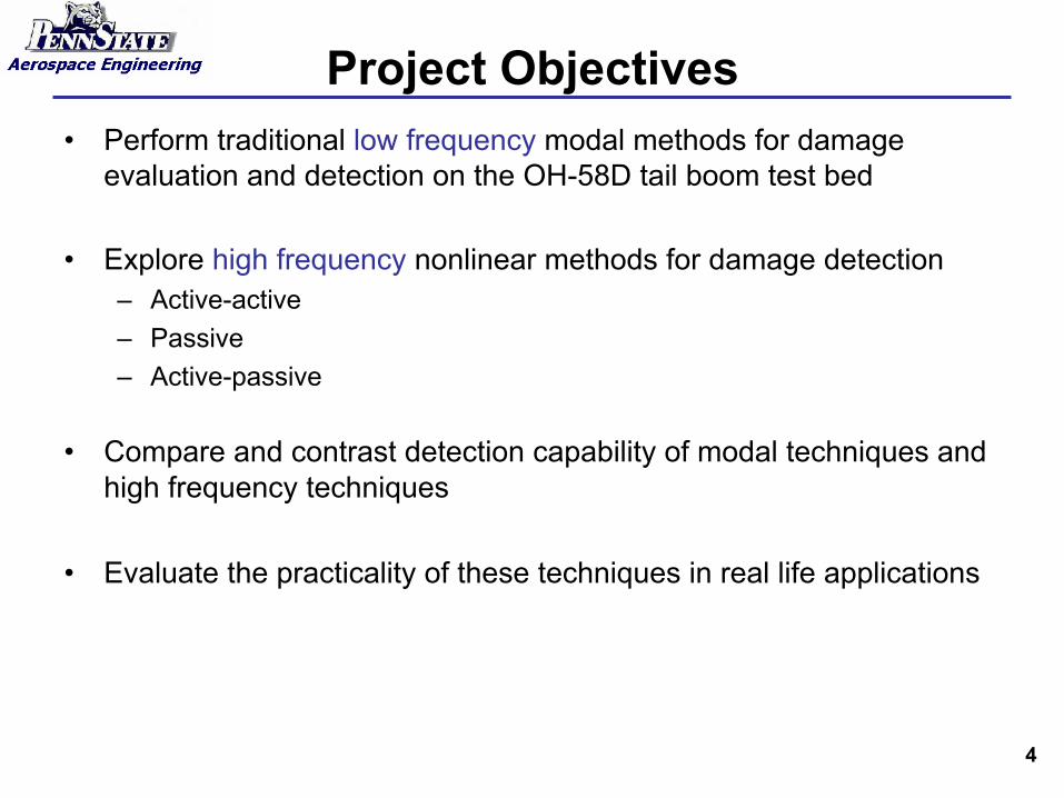
Project Objectives •  Perform traditional low frequency modal methods for damage

evaluation and detection on the OH-58D tail boom test bed

•  Explore high frequency nonlinear methods for damage detection –  Active-active –  Passive –  Active-passive

•  Compare and contrast detection capability of modal techniques and high frequency techniques

•  Evaluate the practicality of these techniques in real life applications

4

Modal Methods

•  Low Frequency Method (0-500 Hz): –  Perform full modal test in healthy and damaged conditions. –  Use full grid of 104 modal points. Extract all modes in bandwidth. –  Compare low-frequency content between healthy and damaged

conditions •  Mid-Frequency Method (0-2000Hz):

–  Perform impact testing at points around damage location. –  Compare frequency response functions (FRFs) between healthy

and damaged conditions

•  Damage is induced by loosening the mid-section hanger bearing bracket.

5

Modal Testing Setup

•  7 accelerometer channels –  Horizontal: 16, 52, 100 –  Vertical: 25, 61, 100 –  Numbers correspond to modal points on tail boom –  104 modal points in all

100 (2 channels)

89 (on stabilizer) 25

16 52

61

Hanger Bearing Bracket Damage Condition

Hit point mesh

6

Modal Results

A number of primary modes were extracted. 7

Full Modal Test Results Second Horizontal Bending Frequency: 17.81 Hz RFP Loss Factor: 0.00449

Second Vertical Bending Frequency: 22.17 Hz RFP Loss Factor: 0.00410

Torsional Mode Frequency: 32.75 Hz RFP Loss Factor: 0.00613

Third Vertical Bending Frequency: 60.67 Hz RFP Loss Factor: 0.0167

8

Modal Results

Some resonance frequencies are very close to tail rotor frequencies. 9

Modal Results

Other resonance frequencies are very close to main rotor frequencies. 10

Modal Results

Accel Damage

11

Mid-Frequency FRF Results

Hit Point Damage Accel

This point showed the most significant deviation between the healthy and damaged condition. Large difference in coherence may indicate damage, but this test is not considered very repeatable.

12

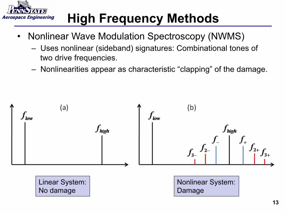
High Frequency Methods •  Nonlinear Wave Modulation Spectroscopy (NWMS)

–  Uses nonlinear (sideband) signatures: Combinational tones of two drive frequencies.

–  Nonlinearities appear as characteristic “clapping” of the damage.

Linear System: No damage

Nonlinear System: Damage

13

High Frequency Methods •  Nonlinear Wave Modulation Spectroscopy (NWMS)

5000 5500 6000 6500 7000 7500 8000 8500 900010-12

10-10

10-8

10-6

10-4

10-2

Frequency (Hz)

Mag

nitu

de ((µ -

S)2 )Auto Power Spectra

Damaged Strain SignalHealthy Strain Signal

In real structures, some nonlinearity is inherent in a healthy condition. More nonlinearity exists in the damaged case. 14

Tail Boom Sensors and Actuators

•  5 accelerometer channels: –  4 in vertical orientation, 1 mounted in horizontal orientation (on bulkhead)

•  7 strain gage channels: –  6 mounted in longitudinal direction, 1 mounted in vertical direction (on bulkhead)

•  2 shakers –  Wilcoxon F4 and F7 (electromagnetic and piezoelectric)

S = strain gage A = accelerometer

1S,1A

1S,1A 1S,1A

1S,1A 1S 1S

1S,1A

F4

F7

15

High Frequency Methods •  Active-Active

–  Two active drive sources at selected frequencies

•  Passive –  Driven frequency consists of natural rotor harmonics

•  Active-Passive –  High driven frequency used in conjunction with rotor

harmonics

16

Active-active Amplitude Studies •  High frequency held at constant 100 V drive voltage

using F7 shaker •  Low frequency amplitude increased to peak value, then

decreased to observe nonlinear characteristics. •  Technique showed best drive condition for exciting

nonlinear response of the damage.

Sensor Damage

Note: Initial studies focused on one sensor, closest to the damage location. 17

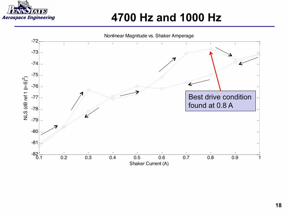
4700 Hz and 1000 Hz

0.1 0.2 0.3 0.4 0.5 0.6 0.7 0.8 0.9 1-82

-81

-80

-79

-78

-77

-76

-75

-74

-73

-72Nonlinear Magnitude vs. Shaker Amperage

Shaker Current (A)

NLS

(dB

ref 1

(µ-S

)2 )

Best drive condition found at 0.8 A

18

Healthy vs. Damaged ∆dB •  Metric represents the change in nonlinear magnitude

between damaged and healthy conditions. •  Positive numbers mean more nonlinear content due to

the damage source. •  All sensors are assessed. Stations 1-7 represent

locations along the tail boom (from aft to forward).

1S,1A

1S,1A 1S,1A

1S,1A 1S 1S

1S,1A 1

3 4 5 6

7 2

19

4700 Hz (100V) and 1000 Hz (0.8A)

Significant increase seen at station 3. May be possible to improve detection sensitivity by changing frequency and/or amplitude

1 2 3 4 5 6 70

1

2

3

4

5

6Nonlinear Strain and Acceleration Healthy vs. Damaged Δ dB

Station

Mag

nitu

de (d

B)

NLA ref 1 (m/s2)2

NLS ref 1 (µ-S)2

20

High Frequency Amplitude Studies •  Low frequency held at constant drive current •  1000 Hz chosen as low frequency •  High frequency amplitude increased to peak

value, then decreased to observe response characteristics.

21

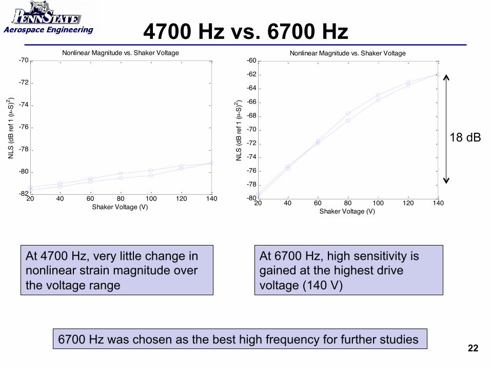
4700 Hz vs. 6700 Hz

20 40 60 80 100 120 140-82

-80

-78

-76

-74

-72

-70Nonlinear Magnitude vs. Shaker Voltage

Shaker Voltage (V)

NLS

(dB

ref 1

(µ-S

)2 )

At 4700 Hz, very little change in nonlinear strain magnitude over the voltage range

20 40 60 80 100 120 140-80

-78

-76

-74

-72

-70

-68

-66

-64

-62

-60Nonlinear Magnitude vs. Shaker Voltage

Shaker Voltage (V)

NLS

(dB

ref 1

(µ-S

)2 )

18 dB

At 6700 Hz, high sensitivity is gained at the highest drive voltage (140 V)

6700 Hz was chosen as the best high frequency for further studies 22

6700 Hz (140V) and 1000 Hz (0.7A)

Good detection sensitivity, especially near damage location. Repeated runs showed similar results. Detection was also possible at other frequencies: A more formal frequency sensitivity study is necessary.

1 2 3 4 5 6 7-1

0

1

2

3

4

5

6

7Nonlinear Strain and Acceleration Healthy vs. Damaged Δ dB

Station

Mag

nitu

de (d

B)

NLA ref 1 (m/s2)2

NLS ref 1 (µ-S)2

23

Rotor Harmonic Passive Study

•  Passive study: input only rotor harmonics –  f1 = 39.7 Hz –  f2 = 79.4 Hz –  f3 = 158.8 Hz –  f4 = 238.2 Hz

•  Drive level of 1 A using F4 shaker •  Analyze changes in total broadband RMS value •  Analyze changes in nonlinear part of broadband

(frequencies higher than driven frequencies)

24

Passive Autospectrum

More higher harmonics are visible in damaged case due to nonlinearity of the damage.

0 500 1000 1500 2000 2500 3000 3500 4000 4500 500010-12

10-10

10-8

10-6

10-4

10-2

100

Frequency (Hz)

Mag

nitu

de ((µ -

S)2 )

Auto Power Spectra: Channel 8 Strain

DamagedHealthy

Highest driven frequency

25

Broadband RMS •  Integrating over the entire broadband spectrum:

0 500 1000 1500 2000 2500 3000 3500 4000 4500 500010-12

10-10

10-8

10-6

10-4

10-2

100

Frequency (Hz)

Mag

nitu

de ((µ -

S)2 )

Auto Power Spectra: Channel 8 Strain

DamagedHealthy

26

Broadband RMS •  Summing over the entire spectrum:

1 2 3 4 5 6 7

0

2

4

6

8

10

12Nonlinear Strain and Acceleration (Broadband) Healthy vs. Damaged Δ dB

Station

Mag

nitu

de (d

B)

NLA ref 1 (m/s2)2

NLS ref 1 (µ-S)2

Low sensitivity to damage, likely because the driven frequencies dominate the response. 27

Higher Harmonic NLA and NLS •  Summing over all frequency content past the driven frequencies:

0 500 1000 1500 2000 2500 3000 3500 4000 4500 500010-12

10-10

10-8

10-6

10-4

10-2

100

Frequency (Hz)

Mag

nitu

de ((µ -

S)2 )

Auto Power Spectra: Channel 8 Strain

DamagedHealthy

Highest driven frequency

28

Higher Harmonic NLS and NLA •  Integrating over all frequency content past the driven frequencies:

1 2 3 4 5 6 70

2

4

6

8

10

12Nonlinear Strain and Acceleration (Higher Harmonic) Healthy vs. Damaged Δ dB

Station

Mag

nitu

de (d

B)

NLA ref 1 (m/s2)2

NLS ref 1 (µ-S)2

Overall very good detection sensitivity using nonlinear components of the passive interrogation. 29

Rotor Harmonics: Active-Passive

•  Tail rotor harmonics input via F4 shaker (1 A) –  f1 = 39.7 Hz –  f2 = 79.4 Hz –  f3 = 158.8 Hz –  f4 = 238.2 Hz

•  High frequency input via F7 shaker (140 V) –  Carrier frequency fhigh = 6700 Hz

•  Observe damaged vs. healthy condition responses

30

Rotor Harmonics: Active-Passive •  Integrating from 4700-6600 Hz and 6800-8700 Hz •  Significant differences between healthy, damaged

conditions in middle stations

1 2 3 4 5 6 70

1

2

3

4

5

6

7

8

9Nonlinear Strain and Acceleration Healthy vs. Damaged Δ dB

Station

Mag

nitu

de (d

B)

NLA ref 1 (m/s2)2

NLS ref 1 (µ-S)2

31

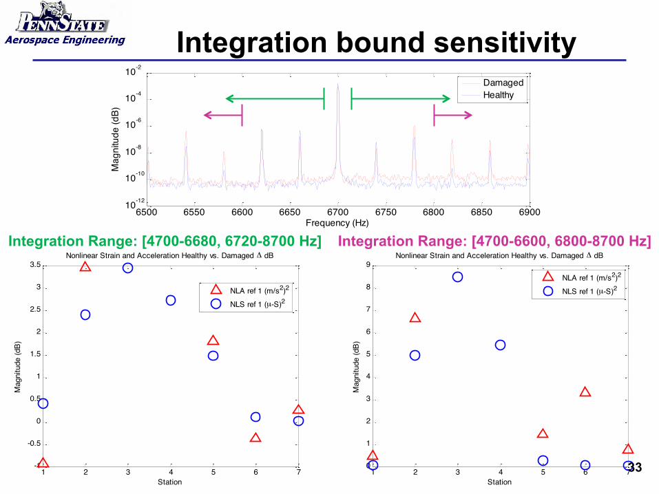
Integration bound sensitivity •  Response magnitude is dominated by bands near 6700 Hz •  Damaged-healthy differences exist beyond the first two sidebands

Frequency response for strain gage from station 3

4000 5000 6000 7000 8000 9000 1000010-12

10-10

10-8

10-6

10-4

10-2

Frequency (Hz)

Mag

nitu

de (d

B)

DamagedHealthy

6500 6550 6600 6650 6700 6750 6800 6850 690010-12

10-10

10-8

10-6

10-4

10-2

Frequency (Hz)

Mag

nitu

de (d

B)

DamagedHealthy

32

Integration bound sensitivity

1 2 3 4 5 6 70

1

2

3

4

5

6

7

8

9Nonlinear Strain and Acceleration Healthy vs. Damaged Δ dB

Station

Mag

nitu

de (d

B)

NLA ref 1 (m/s2)2

NLS ref 1 (µ-S)2

1 2 3 4 5 6 7-1

-0.5

0

0.5

1

1.5

2

2.5

3

3.5Nonlinear Strain and Acceleration Healthy vs. Damaged Δ dB

Station

Mag

nitu

de (d

B)

NLA ref 1 (m/s2)2

NLS ref 1 (µ-S)2

Integration Range: [4700-6680, 6720-8700 Hz] Integration Range: [4700-6600, 6800-8700 Hz]

6500 6550 6600 6650 6700 6750 6800 6850 690010-12

10-10

10-8

10-6

10-4

10-2

Frequency (Hz)

Mag

nitu

de (d

B)

DamagedHealthy

33

Integration bound sensitivity

•  Clearly more nonlinear behavior in the damaged condition vs healthy at station 5

•  Recall that there was little detected difference between healthy and damaged conditions

•  However, the differences do not arise for +/- 400 Hz

6100 6200 6300 6400 6500 6600 6700 6800 6900 7000 7100 7200 7300

10-8

10-6

10-4

10-2

100

102

Frequency (Hz)

Mag

nitu

de (d

B)

DamagedHealthy

34

6700 Hz (140V) and 1000 Hz (1A)

1 2 3 4 5 6 70

1

2

3

4

5

6

7

8

9Nonlinear Strain and Acceleration Healthy vs. Damaged Δ dB

Station

Mag

nitu

de (d

B)

NLA ref 1 (m/s2)2

NLS ref 1 (µ-S)2

•  Changing the integration band brings out the station 5 difference (+10 db vs +2 db)

•  Damage sensitivity is highly dependent upon integration bounds

•  Further investigation into integration algorithm needed

1 2 3 4 5 6 70

2

4

6

8

10

12

14

16

18

20Nonlinear Strain and Acceleration Healthy vs. Damaged Δ dB

Station

Mag

nitu

de (d

B)

NLA ref 1 (m/s2)2

NLS ref 1 (µ-S)2

Integration Range: [4700-6600, 6800-8700 Hz] Integration Range: [4700-6200, 7200-8700 Hz]

35

Conclusions •  Low frequency methods were useful for determining potential

causes of fatigue damage. However, linear methods were not capable of detecting damage on the scale of the hanger bearing bracket.

•  Mid- frequency measurements were not conclusive, using a force hammer for excitation. This method may be more effective using a shaker for force input.

•  High frequency methods were effective for detecting the damage condition. Further studies should focus on optimizing drive conditions and spectral processing techniques. Active-active, passive and active-passive techniques all show promise for potential integration in real airframe structures.

36

Structural Health Monitoring 1.75 in

10000 Hz, 1/2 𝜆= 0.6 in

1000 Hz, 1/2 𝜆= 2 in

100 Hz, 1/2 𝜆= 6 in

10 Hz, 1/2 𝜆= 20 in

Typically, the best detection capability results from using vibration wavelengths on the order of the damage size. 37