Aircraft Dynamics

First order and Second order system

Prepared

by

A.Kaviyarasu

Assistant Professor

Department of Aerospace Engineering

Madras Institute Of Technology

Chromepet, Chennai

Aircraft dynamic stability focuses on the time history of aircraftmotion after the aircraft is disturbed from an equilibrium or trimcondition.

This motion may be first order (exponential response) or secondorder (oscillatory response), and will have

Positive dynamic stability (aircraft returns to the trim condition astime goes to infinity).

Neutral dynamic stability (aircraft neither returns to trim nordiverges further from the disturbed condition).

Dynamic instability (aircraft diverges from the trim condition andthe disturbed condition as time goes to infinity).

The study of dynamic stability is important to understanding

aircraft handling qualities and the design features that make

an airplane fly well or not as well while performing specific

mission tasks.

The differential equations that define the aircraft equations of

motion (EOM) form the starting point for the study of

dynamic stability.

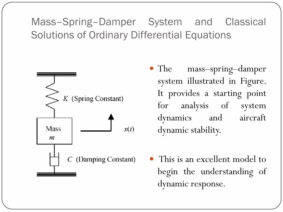
Mass–Spring–Damper System and Classical

Solutions of Ordinary Differential Equations

The mass–spring–damper

system illustrated in Figure.

It provides a starting point

for analysis of system

dynamics and aircraft

dynamic stability.

This is an excellent model to

begin the understanding of

dynamic response.

We will first develop an expression for the sum of forces in the vertical direction.

Notice that x(t) is defined as positive for an upwarddisplacement and that the zero position is chosen as the pointwhere the system is initially at rest or at equilibrium. Weknow that

There are two forces acting on the mass, the damping force,and the spring force.

2

2x

d xF m

dt

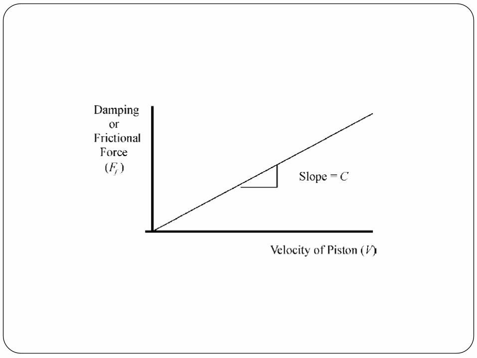
For the damping or frictional force this can be approximatedby a linear relationship of damping force as a function of velocityor

A damper can be thought of as a ‘‘shock absorber’’ with a pistonmoving up and down inside a cylinder. The piston is immersed in afluid and the fluid is displaced through a small orifice to provide aresistance force directly proportional to the velocity of the piston.

This resistance force can be expressed as

where C is the slopefF CV

fF

fF

dxdt

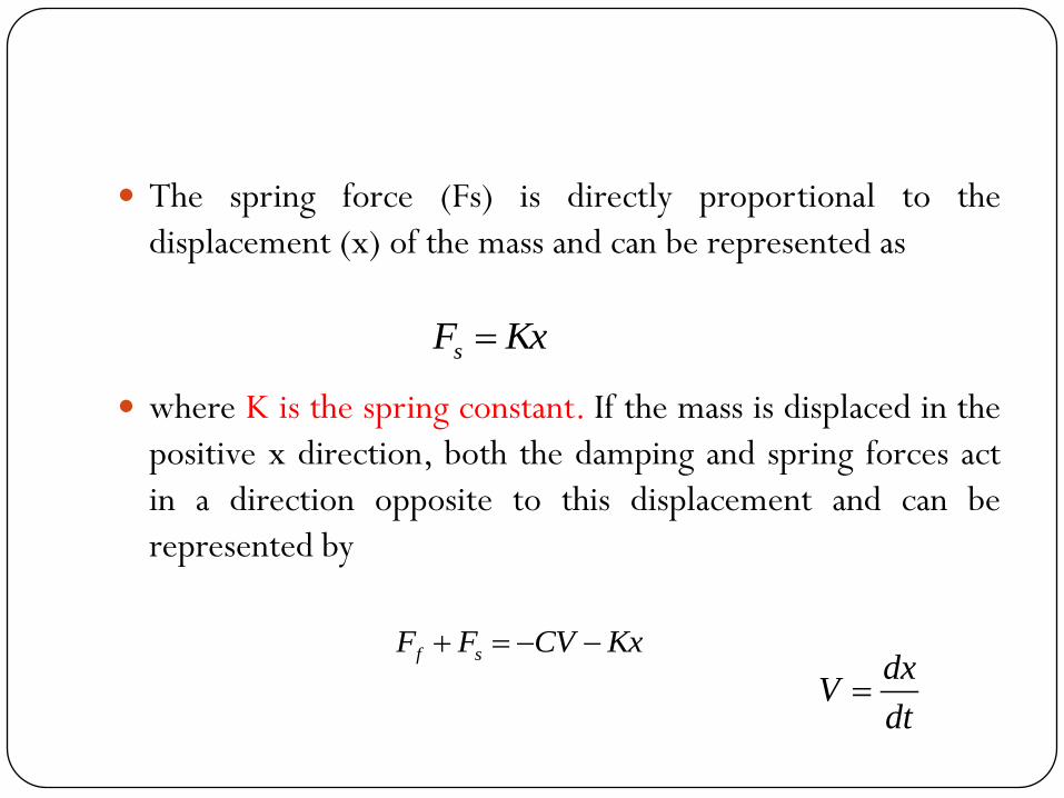
The spring force (Fs) is directly proportional to the

displacement (x) of the mass and can be represented as

where K is the spring constant. If the mass is displaced in the

positive x direction, both the damping and spring forces act

in a direction opposite to this displacement and can be

represented by

sF Kx

f sF F CV Kx dx

Vdt

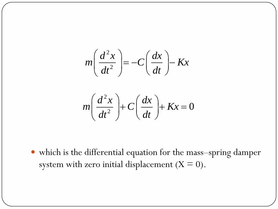
which is the differential equation for the mass–spring damper

system with zero initial displacement (X = 0).

2

2

d x dxm C Kx

dt dt

2

20

d x dxm C Kx

dt dt

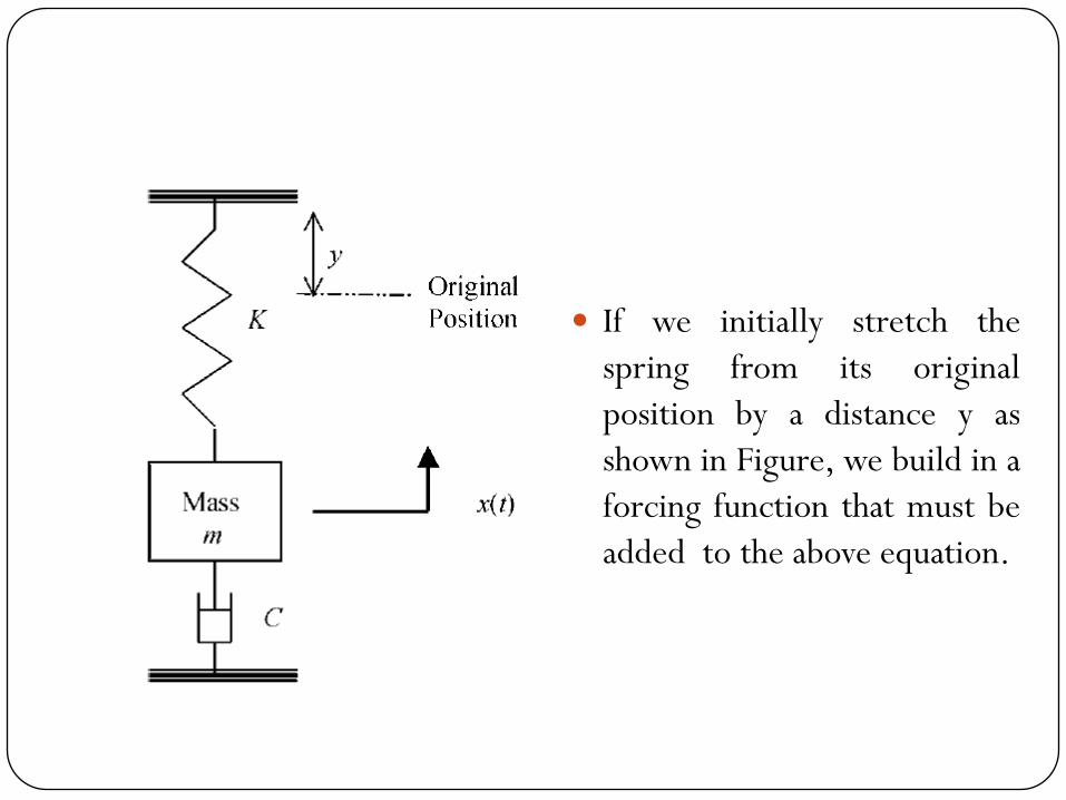
If we initially stretch the

spring from its original

position by a distance y as

shown in Figure, we build in a

forcing function that must be

added to the above equation.

This is the differential equation for the spring–mass–damper systemwith applied force externally. At this point, we should observe that ifthe mass is free to move, it will obtain a steady-state condition (a newequilibrium location) when equal zero and the newequilibrium position will be x= y.

But the system will take certain amount of time to come back itsoriginal position because of the presence of spring and damper.

It is also representative of aircraft motion and that is why we areinvestigating it in depth.

2

2

d x dxm C Kx Ky

dt dt

2

2 d x dxanddtdt

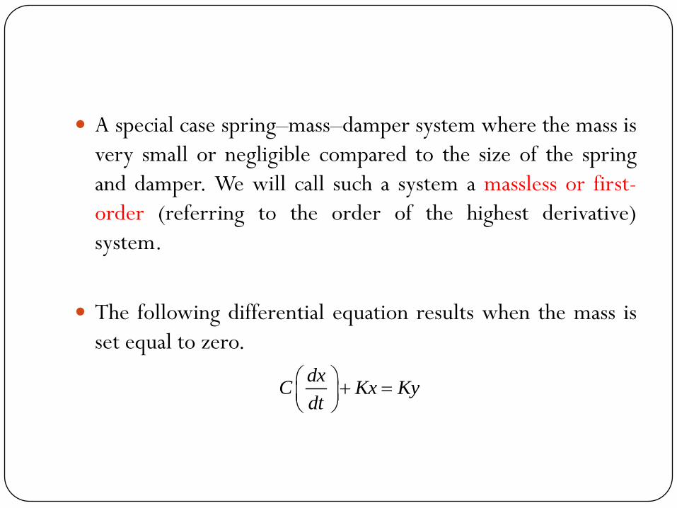
A special case spring–mass–damper system where the mass is

very small or negligible compared to the size of the spring

and damper. We will call such a system a massless or first-

order (referring to the order of the highest derivative)

system.

The following differential equation results when the mass is

set equal to zero.

dxC Kx Ky

dt

22

2

dx d x xPx P x xdt

dt dt p

0dx

C Kxdt

0CPx Kx

0CP K x

KP

C

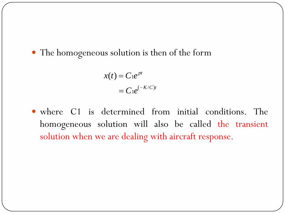
The homogeneous solution is then of the form

where C1 is determined from initial conditions. The

homogeneous solution will also be called the transient

solution when we are dealing with aircraft response.

1

/1

( )

pt

K C t

x t C e

C e

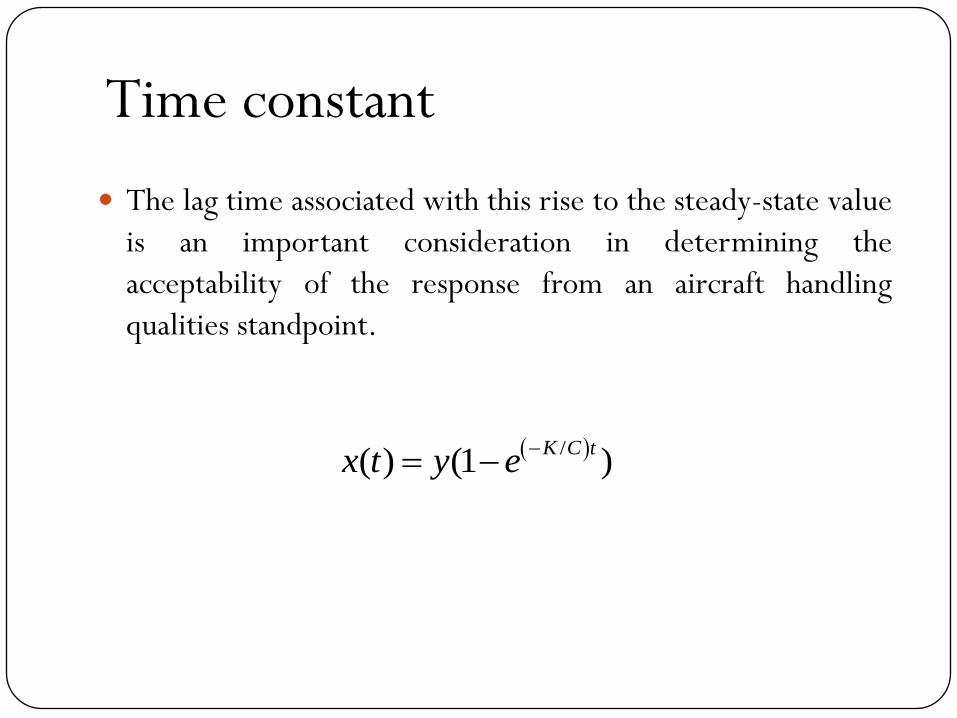
Time constant

The lag time associated with this rise to the steady-state value

is an important consideration in determining the

acceptability of the response from an aircraft handling

qualities standpoint.

/( ) (1 )

K C tx t y e

This lag time is typically quantified with the time constant

which is a measure of the time it takes to achieve 63.2% of

the steady-state value.

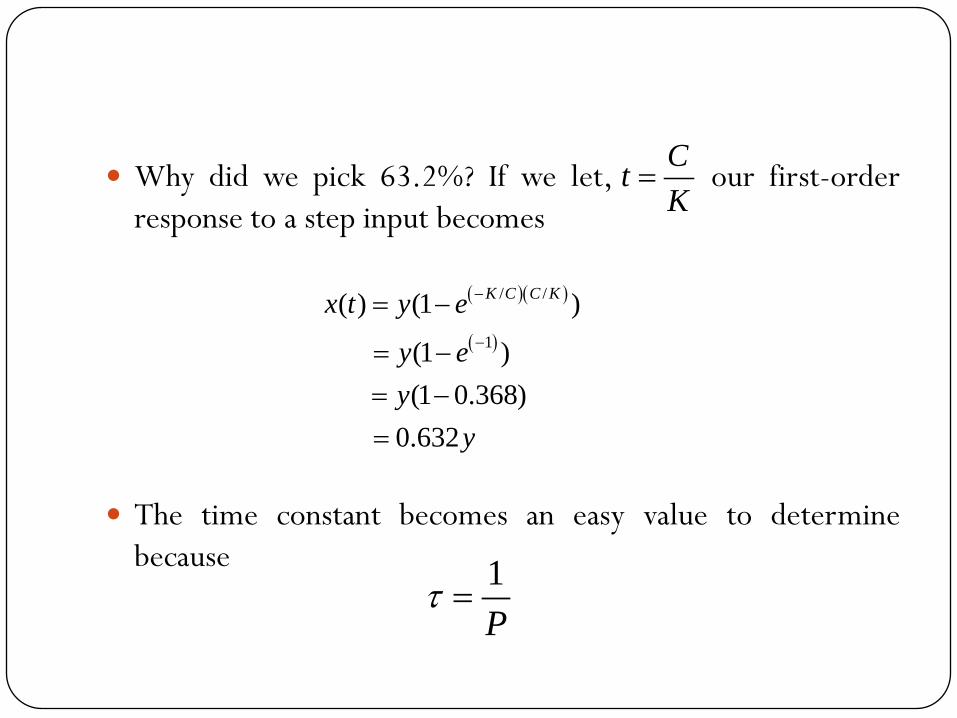
Why did we pick 63.2%? If we let, our first-order

response to a step input becomes

The time constant becomes an easy value to determine

because1

P

Ct

K

/ /

1

( ) (1 )

(1 )

(1 0.368)

0.632

K C C Kx t y e

y e

y

y

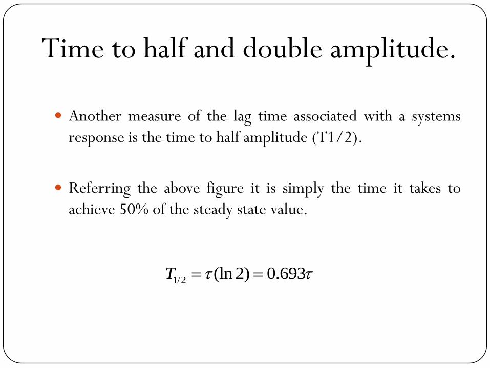
Time to half and double amplitude.

Another measure of the lag time associated with a systems

response is the time to half amplitude (T1/2).

Referring the above figure it is simply the time it takes to

achieve 50% of the steady state value.

1/2 (ln 2) 0.693T

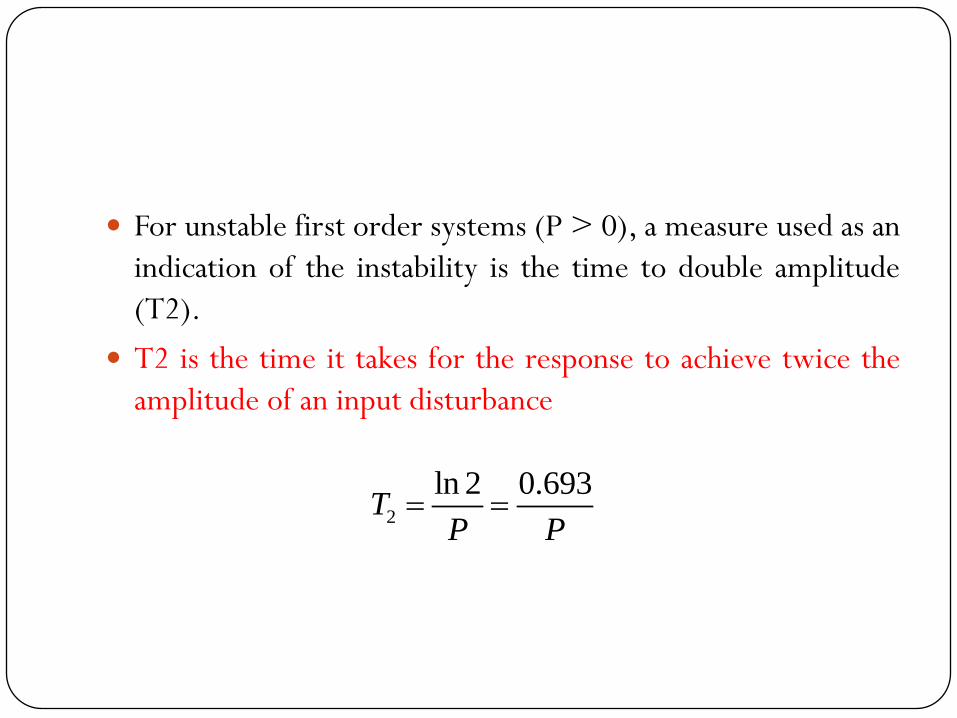
For unstable first order systems (P > 0), a measure used as an

indication of the instability is the time to double amplitude

(T2).

T2 is the time it takes for the response to achieve twice the

amplitude of an input disturbance

2

ln 2 0.693T

P P

Note also, because is equal to C/K for the spring–mass–damper system.

will increase (meaning a slower responding system) for anincrease in damping constant (C)

will decrease (meaning a faster responding system) for anincrease in the spring constant (K).

This should make sense when thinking about the physicaldynamics of the system.

Second order system

Spring–mass–damper system where the mass provides

significant inertial effects.

The second order Spring-mass-damper has been written as

We can solve the roots by using quadratic equation formula

2

1,2

4

2 2

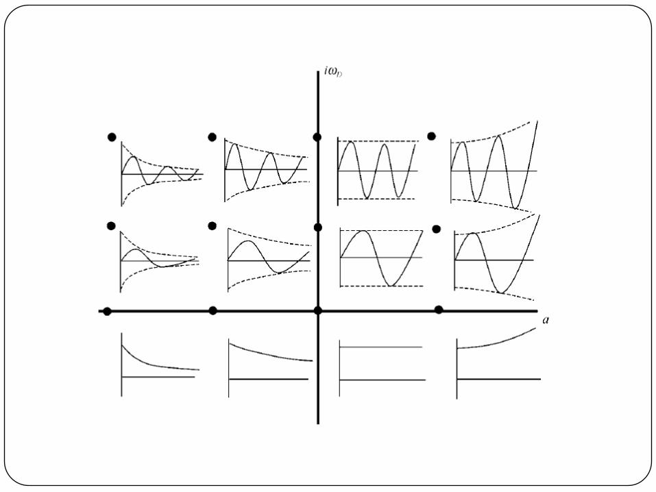
C KM CP i a ib

M M

2 ( ) 0Mx Cx Kx Ky or MP CP K x

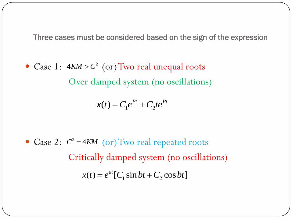
Three cases must be considered based on the sign of the expression

Case 1: (or) Two real unequal roots

Over damped system (no oscillations)

Case 2: (or) Two real repeated roots

Critically damped system (no oscillations)

24KM C

2 4C KM

1 2( ) Pt Ptx t C e C te

1 2( ) [ sin cos ]atx t e C bt C bt

Case 3: (or) Two real repeated roots

Under damped system (with oscillations) system.

24KM C

2

1,2

4

2 2

C KM CP i a ib

M M

1 2 ( ) [ sin cos ]atGeneral solution x t e C bt C bt

Second order system We can rewrite the second order system in the form of

The damping ratio provides an indication of the system dampingand will fall between -1 and 1.

For stable systems, the damping ratio will be between 0 and 1.

For this case, the higher the damping ratio, the more damping ispresent in the system.

2 22

N N N

N

x x x y where damping ratio

natural frequency

Notice that the number of overshoots/undershoots varies

inversely with the damping ratio.

The natural frequency is the frequency (in rad/s) that the

system would oscillate at if there were no damping.

Natural Frequency

The natural frequency is the frequency (in rad/s) that

the system would oscillate at if there were no damping. It

represents the highest frequency that the system is capable of,

but it is not the frequency that the system actually oscillates

at if damping is present.

For the mass–spring–damper system the natural frequency

oscillation /N K M

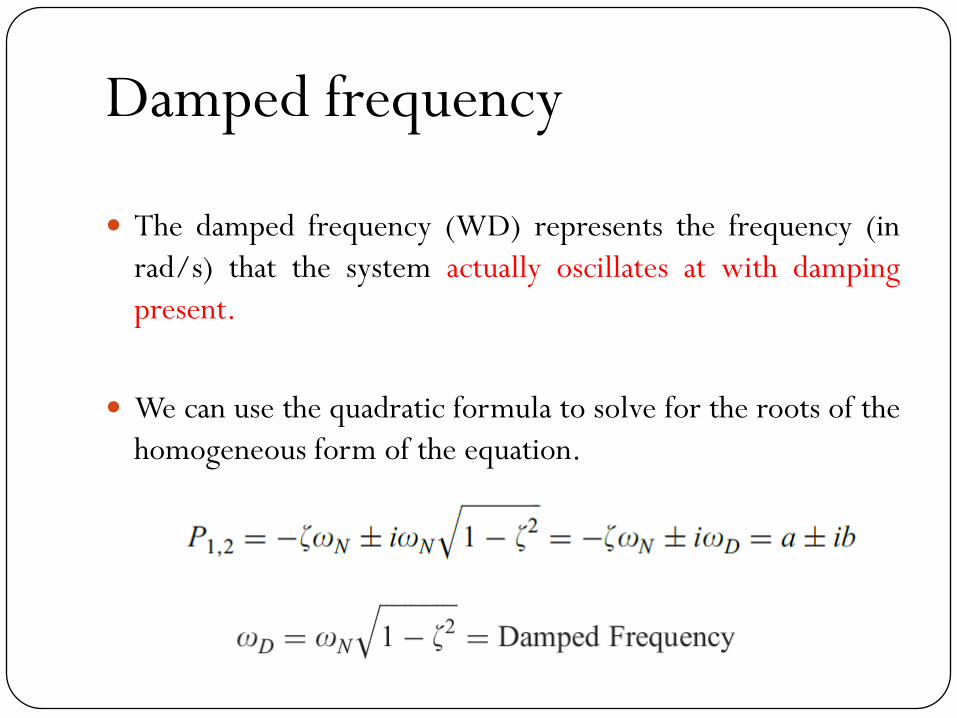
Damped frequency

The damped frequency (WD) represents the frequency (in

rad/s) that the system actually oscillates at with damping

present.

We can use the quadratic formula to solve for the roots of the

homogeneous form of the equation.

The time constant of a second order system

Notice that larger the value of will smaller time constant

will increases faster response.

It is similar to calculate the time constant of a first order

system

1

n

1

pole

n

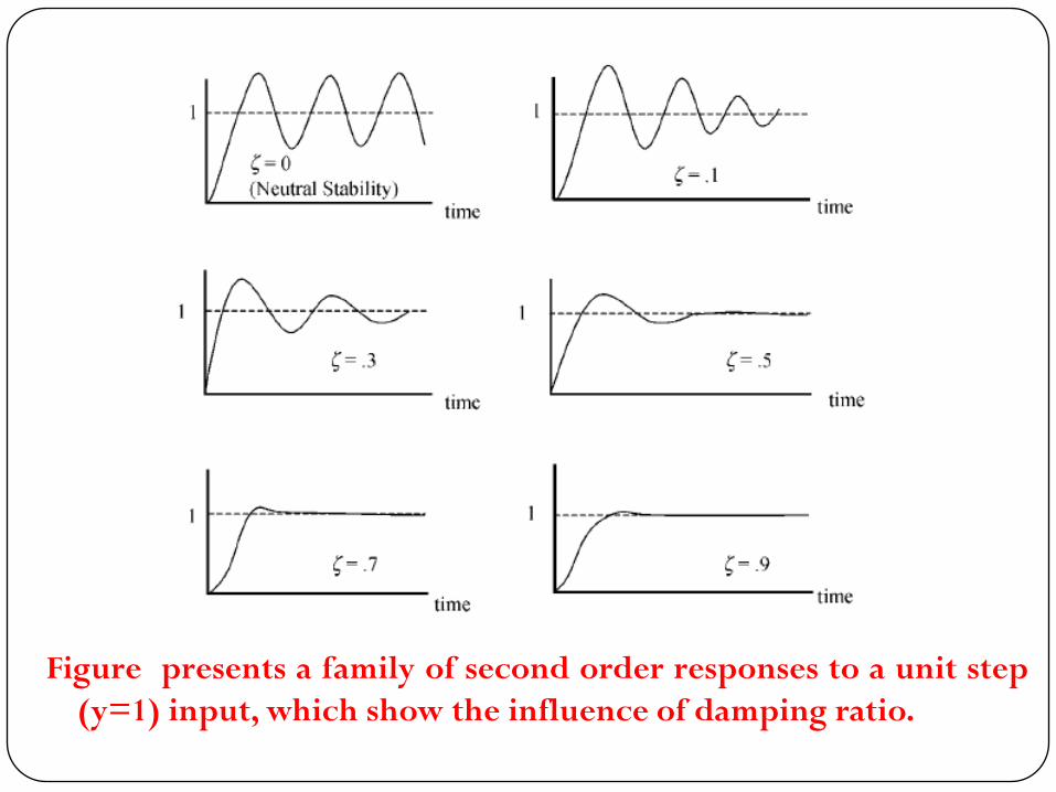
Figure presents a family of second order responses to a unit step

(y=1) input, which show the influence of damping ratio.

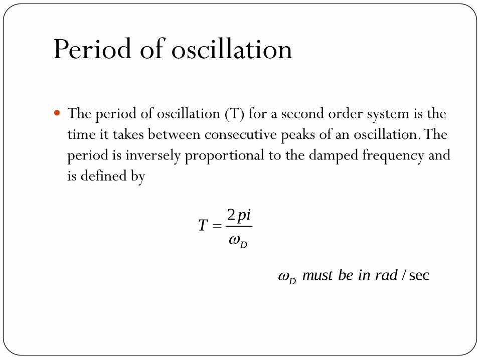
Period of oscillation

The period of oscillation (T) for a second order system is the

time it takes between consecutive peaks of an oscillation. The

period is inversely proportional to the damped frequency and

is defined by

2

D

piT

/ secD must be in rad

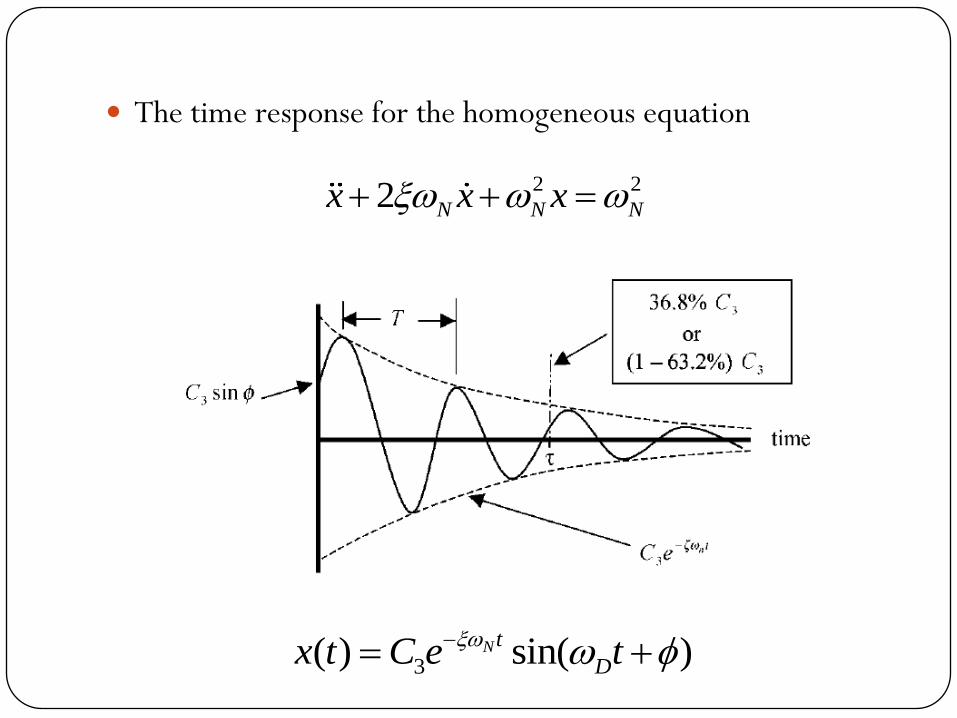
The time response for the homogeneous equation

3( ) sin( )N t

Dx t C e t

2 22 N N Nx x x

Thank you