Air Velocity Anemometer Lab

Air Velocity Measurements with a Hot Wire Anemometer

[ ] April 11, 2013

Abstract:

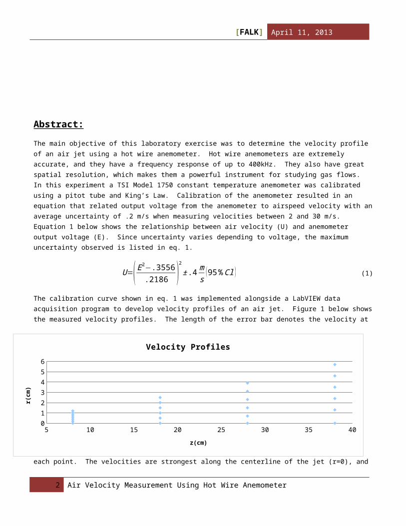
The main objective of this laboratory exercise was to determine the velocity profile of an air jet using a hot wire anemometer. Hot wire anemometers are extremely accurate, and they have a frequency response of up to 400kHz. They also have great spatial resolution, which makes them a powerful instrument for studying gas flows. In this experiment a TSI Model 1750 constant temperature anemometer was calibrated using a pitot tube and King’s Law. Calibration of the anemometer resulted in an equation that related output voltage from the anemometer to airspeed velocity with an average uncertainty of .2 m/s when measuring velocities between 2 and 30 m/s. Equation 1 below shows the relationship between air velocity (U) and anemometer output voltage (E). Since uncertainty varies depending to voltage, the maximum uncertainty observed is listed in eq. 1.

U=( E2−.3556.2186 )

2

± .4ms

(95 %Cl ) (1)

The calibration curve shown in eq. 1 was implemented alongside a LabVIEW data acquisition program to develop velocity profiles of an air jet. Figure 1 below shows the measured velocity profiles. The length of the error bar denotes the velocity at each point. The velocities are strongest along the centerline of the jet (r=0), and they taper off as r and z variables increase. The points on the outside edge of each profile were then used to determine the jet angle using linear regression. The

Figure 1: Velocity Profiles

calculated value for this angle is 6.7± .2° (95%Cl ) . The orifice diameter was also approximated using the y-intercept fro

m the regression equation. This value is.2± .4 cm(95%Cl). The uncertainty for this approximation is quite high when compared to the actual measurement. To reduce uncertainty in future research, more data points at different z locations should be used since the uncertainty is dependent on regression fit quality.

The final area of study in this experiment was turbulence intensity. The turbulence intensity at any given point is given by dividing the standard deviation of the velocities measured at a point by the mean centerline velocity at the particular z location. As the z distance from the jet increased, turbulence intensity increased. As the r distance from the centerline increased, turbulence intensity seemed to increase and then drop off as the edge of the jet is approached. The amount of data points limited the accuracy of the results in this section. Future studies in this area should use many more data points.

2 Air Velocity Measurement Using Hot Wire Anemometer

5 10 15 20 25 30 35 400

1

2

3

4

5

6

Velocity Profiles

z(cm)

r(cm

)

[ ] April 11, 2013

Introduction:

The purpose of this experiment was to develop multiple velocity profiles along the span of an air jet using a hot wire anemometer. Hot wire anemometers use an extremely thin, exposed wire element through which an electric current flows. They are extremely accurate and responsive, and are often utilized in research applications. They are often impractical to use in industrial applications mainly because they are fragile, costly, and can only be used in clean gasses. They also require frequent calibrations, and need to be calibrated even more frequently in unclean gasses. Nonetheless, they are one of the most accurate ways of measuring gas velocity.

The particular anemometer that was used in this experiment varied voltage across the wire to keep it at a constant temperature. This voltage was converted to an airspeed using King’s Law and a pitot tube to provide the reference air velocities at different points. A pitot tube measures air velocity by examining the difference between static and total pressures at a particular point in an air flow. A manometer was used in conjunction with the pitot tube to read the pressure differential between static and total air pressures. It uses a fluid of known density and a graduated tube to calculate the pressure differential based on the change in fluid height in the tube. The particular manometer used in this experiment was angled to provide higher resolution in measurement.

Experimental Methods: Overview:The hot wire anemometer was calibrated using calculated air velocity values from a pressure differential measured by an inclined manometer. The Pitot tube was placed at a designated location and the airspeed was increased until a certain pressure differential was achieved. The hot wire anemometer was then moved into the same position as the Pitot tube was and a voltage measurement was sampled using a LabVIEW data acquisition program. The pressure differential from the manometer was also recorded with the sampled voltage to create a single data point. The air velocity (U) can be calculated from the manometer using equation 2 below where ∆ P is the pressure differential, R is the specific gas constant for air, and

p is the ambient air pressure.

U=√( 2 (∆P ) (R ) (T ) )/ p ¿¿ (eq. 2)

A plot of E2vs √U was then created and linear regression was performed on the data points which resulted in the King’s Law

relationship between voltage (E) and air velocity (U). The general form of King’s law is shown below in eq. 3.

E2=A+B √U (eq. 3)

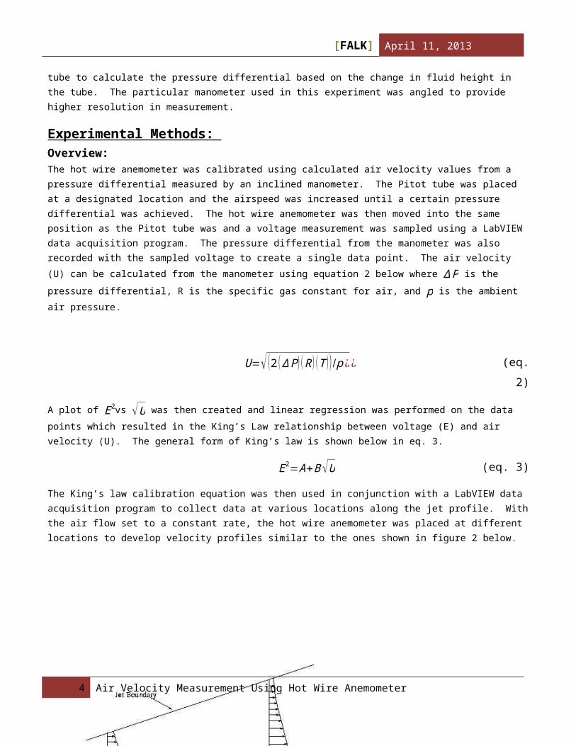
The King’s law calibration equation was then used in conjunction with a LabVIEW data acquisition program to collect data at various locations along the jet profile. With the air flow set to a constant rate, the hot wire anemometer was placed at different locations to develop velocity profiles similar to the ones shown in figure 2 below.


z

r

[ ] April 11, 2013

Figure2: sample velocity profiles

The outer edges of each velocity profile are where the velocity is equal to 20% of the mean centerline velocity at that z location. These points were used to create a profile of the jet boundary, which allowed the calculation of the jet angle. A linear regression was performed on the jet boundary points, and the inverse tangent of the regression slope is equal to the jet angle. Furthermore, the jet orifice diameter could be approximated using the jet boundary line. This approximation can be accomplished by multiplying the y-intercept of the regression line by 2.

The final portion of this experiment examined the turbulence intensity at each of the points in the examined velocity profiles. Turbulence intensity can be calculated using equation 4 below.

TI= u'

UCL

(eq.4)

Where TI is turbulence intensity, u’ is the standard deviation of the sampled velocities at a point, and UCL is the mean

centerline velocity at that z location.

Apparatus & Equipment:

Table 1 shows the measurement equipment used.

Equipment Table

ItemManufacturer

Model No. Serial No. Accuracy

Pitot tube Inclined Manometer Dwyer 0.25%Adjustable Blower and Nozzle Hotwire Probe

TSI Model 1750 CT Anemometer TSI 17507112003

6 Digital Oscilloscope DAQ TI USB-6008

Table 1: Equipment used


[ ] April 11, 2013

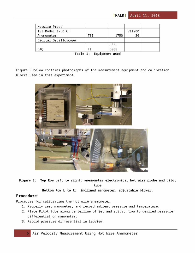
Figure 3 below contains photographs of the measurement equipment and calibration blocks used in this experiment.

Figure 3: Top Row Left to right: anemometer electronics, hot wire probe and pitot tubeBottom Row L to R: inclined manometer, adjustable blower.

Procedure: Procedure for calibrating the hot wire anemometer:

1. Properly zero manometer, and record ambient pressure and temperature.2. Place Pitot tube along centerline of jet and adjust flow to desired pressure differential on manometer. 3. Record pressure differential in LabView. 4. Move hot wire probe to centerline of jet and acquire voltage sample using LabVIEW data acquisition program. 5. Repeat 2-4 until desired amount of data points are collected over desired range of air velocities. 6. Perform linear regression on data points to achieve calibration curve using data analysis software eq. 2, and eq. 3.

Procedure for measuring spatial velocity and turbulence:1. Set hotwire probe to desired z location along centerline of jet, record this location. 2. Acquire Voltage/Velocity measurement and calculate 20% of the velocity measurement. 3. Move the hotwire probe in the r direction until the desired 20% measurement is shown. Record r and z locations in

LabVIEW software and acquire data point.4. Move hotwire probe in even increments back to centerline, acquiring data points at each location.

5. Once all desired data points taken at that particular z location. Move to the next desired z location and repeat steps 2-4. Make sure to use even spacing and the same number of data points for each z location.


[ ] April 11, 2013

Results and Discussion

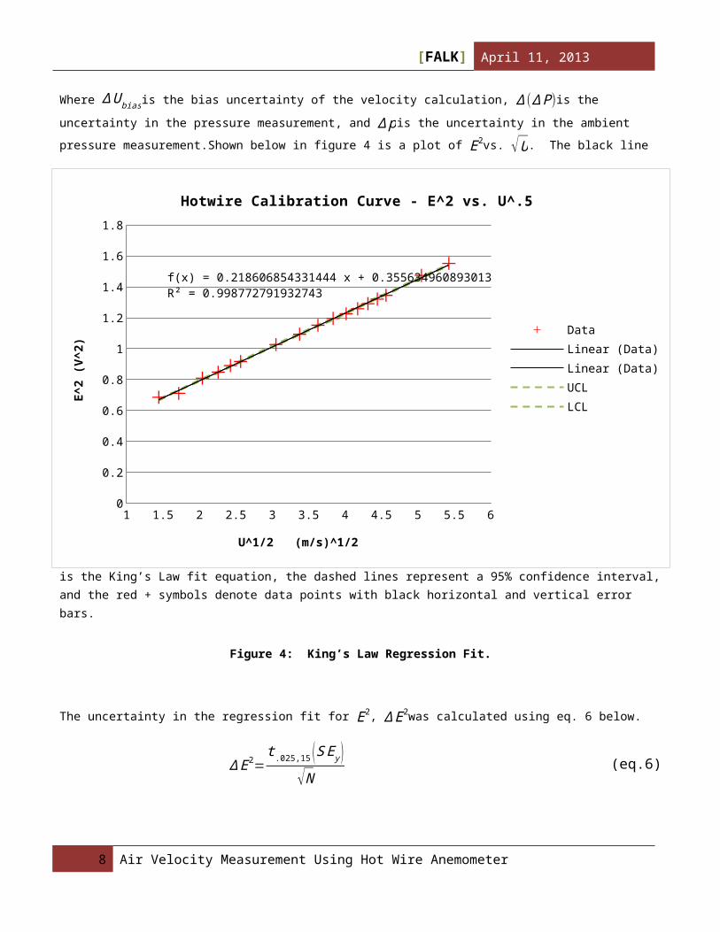
Part 1 – Hotwire Anemometer Calibration:This section discusses the methods used for calibrating the hotwire anemometer. It discusses how air velocity was calculated

using the Pitot tube pressure differential as well as the uncertainty propagation for the calculation. A plot of E2vs. √U is

also included which is shown in figure 4. This section also shows the calculated calibration equation from regression, as well as the uncertainty propagation for U.

To calculate the air velocity from the pitot tube pressure differential, eq. 2 (above) was used. The uncertainty propagation equation below (eq. 5) shows how the bias uncertainty in the velocity measurement was calculated.

∆U bias=√( ∂U∂ ∆P

∆(∆ P))2

+( ∂U∂ p∆ p)

2

(5)

Where ∆U biasis the bias uncertainty of the velocity calculation, ∆ (∆ P)is the uncertainty in the pressure measurement, and

∆ pis the uncertainty in the ambient pressure measurement.Shown below in figure 4 is a plot of E2vs. √U . The black line is

the King’s Law fit equation, the dashed lines represent a 95% confidence interval, and the red + symbols denote data points with black horizontal and vertical error bars.


1 1.5 2 2.5 3 3.5 4 4.5 5 5.5 60

0.2

0.4

0.6

0.8

1

1.2

1.4

1.6

1.8

f(x) = 0.218606854331444 x + 0.355634960893013R² = 0.998772791932743

Hotwire Calibration Curve - E^2 vs. U^.5

DataLinear (Data)Linear (Data)UCLLCL

U^1/2 (m/s)^1/2

E^2

(V^2

)

[ ] April 11, 2013

Figure 4: King’s Law Regression Fit.

The uncertainty in the regression fit for E2, ∆ E2was calculated using eq. 6 below.

∆ E2=t.025,15 (S E y )

√N (eq.6)

Where t .025,15 is the calculated t-value for regression fit with degrees of freedom N-2, S Ey is the standard error of the

regression fit for E2, and N is the sample size.

The uncertainty calculated in eq. 6 was then propagated to determine the regression uncertainty in the calculated air velocity

(∆U ) using eq. 7 below.

∆U reg=∂U

∂ E2∆ E2

(eq. 7)

The regression uncertainty and bias uncertainty in the air velocity measurement can then be combined using the RSS method, which is shown in eq. 8.

∆U tot=√∆U bias2+∆U reg

2 (eq.8)

The final calibration equation is shown below in eq. 9. The uncertainty varies for each point due to varying bias uncertainty

as well as varying values of E2 at the different data points. The maximum uncertainty is shown in eq. 9.

U=( E2−.3556.2186 )

2

± .4ms

(95 %Cl ) (eq. 9)

The r2value of the regression equation is .9988, which means there is a high level of accuracy in the fit equation. Most of the

uncertainty comes from the propagation of error and a small contribution from the bias error in the pressure measurements.

Part 2 – Velocity Profile and Jet Angle:

This section illustrates the process that was used to determine the velocity profiles at each of four z locations, as well as their respective uncertainties. Also discussed in this section are the methods used to calculate the jet angle and uncertainty propagation for this calculation. Finally, the approximation of orifice diameter and its respective uncertainty is discussed.

Shown below in figure 5 is a plot of the measured velocity profiles. The origin denotes the mouth and center of the jet. The data points are the spatial locations where the measurements were made, and the error bars show the velocity magnitudes. The velocity magnitudes can be located using the table to the left of figure 5.


[ ] April 11, 2013

Figure 5: Velocity ProfilesIt can be clearly seen that the velocity is greatest along the centerline of the jet, and

that it decreases as the z distance from the jet increases. Air velocity also decreases as r distance from centerline increases. There is also a clear angle at which the jet widens as z increases.To calculate the jet angle, the velocities at the highest r values of each z location can be plotted. A linear regression can then be performed on the data. By using simple trigonometry, it can be seen that the slope of the regression line is equal to the tangent of the jet angle. Eq. 10 shows this equation solved for jet angle (θ).

θ=tan−1m (eq. 9)

The uncertainty in the jet angle can be propagated from the uncertainty in the regression fit. Eq. 10 shows the propagation equation for uncertainty in the jet angle.

∆θ= ∂θ∂m

∆m=

1

1+m2 ( t.025,2 )S Em

√N(eq. 10)


5 10 15 20 25 30 35 400

1

2

3

4

5

6

Velocity Profiles

z(cm)

r(cm

)

Z (cm) r (cm) Velocity(m/s)

8 0 11.2

8 1.2 2.6

8 1 4.4

8 0.8 5.5

8 0.6 7.6

8 0.4 10.3

8 0.2 11.0

18 0 5.9

18 2.5 1.2

18 2 2.0

18 1.5 3.2

18 1 4.1

18 0.5 5.3

28 0 3.8

28 3.9 0.7

28 3.1 1.2

28 2.3 1.9

28 1.5 2.7

28 0.7 3.1

38 0 2.6

38 5.7 0.3

38 4.6 0.4

38 3.5 1.6

38 2.4 1.6

38 1.3 2.8

[ ] April 11, 2013

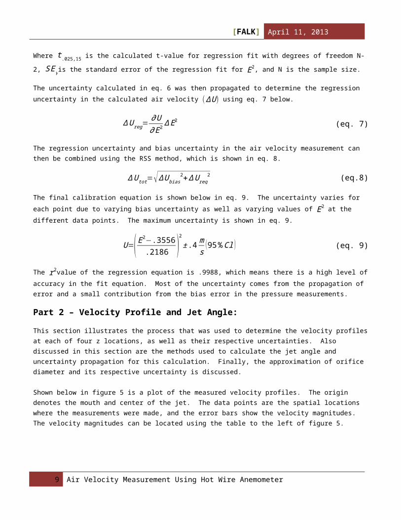
Utilizing these equations, the calculated jet angle is 6.6± .2°(95%Cl). This is a feasible jet angle calculation, and the uncertainty is quite low.

The regression line from the jet angle calculations can also be used to approximate the orifice diameter(D). To do this, the y-intercept of the regression line simply needs to be multiplied by a factor of 2. The uncertainty of this can be calculated using eq. 11.

∆ D=∂D∂b

∆b=2 (S Eb ) (eq.11)

The calculated value for the orifice diameter is .2± .4 cm(95%Cl). One can easily see that the uncertainty in the measurement is greater than the size of the measurement itself, which renders this calculation to be only useful as an approximation.

Part 3 –Turbulence Intensity:

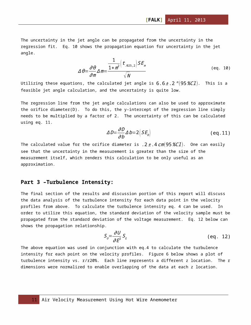
The final section of the results and discussion portion of this report will discuss the data analysis of the turbulence intensity for each data point in the velocity profiles from above. To calculate the turbulence intensity eq. 4 can be used. In order to utilize this equation, the standard deviation of the velocity sample must be propagated from the standard deviation of the voltage measurement. Eq. 12 below can shows the propagation relationship.

SU=∂U

∂ E2SE (eq. 12)

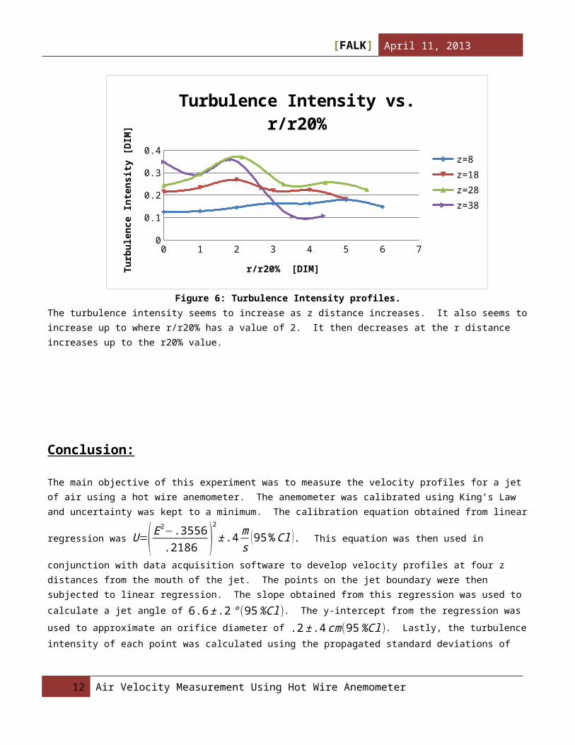
The above equation was used in conjunction with eq.4 to calculate the turbulence intensity for each point on the velocity profiles. Figure 6 below shows a plot of turbulence intensity vs. r/r20%. Each line represents a different z location. The r dimensions were normalized to enable overlapping of the data at each z location.

Figure 6: Turbulence Intensity profiles.The turbulence intensity seems to increase as z distance increases. It also seems to increase up to where r/r20% has a value of 2. It then decreases at the r distance increases up to the r20% value.


0 1 2 3 4 5 6 70

0.05

0.1

0.15

0.2

0.25

0.3

0.35

0.4

Turbulence Intensity vs. r/r20%

z=8z=18z=28z=38

r/r20% [DIM]

Turb

ulen

ce In

tens

ity [D

IM]

[ ] April 11, 2013

Conclusion:

The main objective of this experiment was to measure the velocity profiles for a jet of air using a hot wire anemometer. The anemometer was calibrated using King’s Law and uncertainty was kept to a minimum. The calibration equation obtained

from linear regression was U=( E2−.3556.2186 )

2

± .4ms

(95 %Cl ). This equation was then used in conjunction with data

acquisition software to develop velocity profiles at four z distances from the mouth of the jet. The points on the jet boundary were then subjected to linear regression. The slope obtained from this regression was used to calculate a jet angle of

6.6± .2° (95%Cl). The y-intercept from the regression was used to approximate an orifice diameter of

.2± .4 cm(95%Cl). Lastly, the turbulence intensity of each point was calculated using the propagated standard deviations of the velocity samples. The plot in figure 6 illustrates the turbulence intensity profiles.

Uncertainties were calculated using the standard partial derivative method. Precision and bias uncertainties were combined using the root sum of squares method. One of the main sources of error in this experiment comes from the measurement of the r and z locations of the anemometer. Another source of error was the positioning of the Pitot tube and anemometer in the centerline of the jet for calibration. In future studies, more data points should be taken for velocity profiles to lessen the uncertainty from regression.


[ ] April 11, 2013

References:

[1] ME 4031W Lab Manual


[ ] April 11, 2013

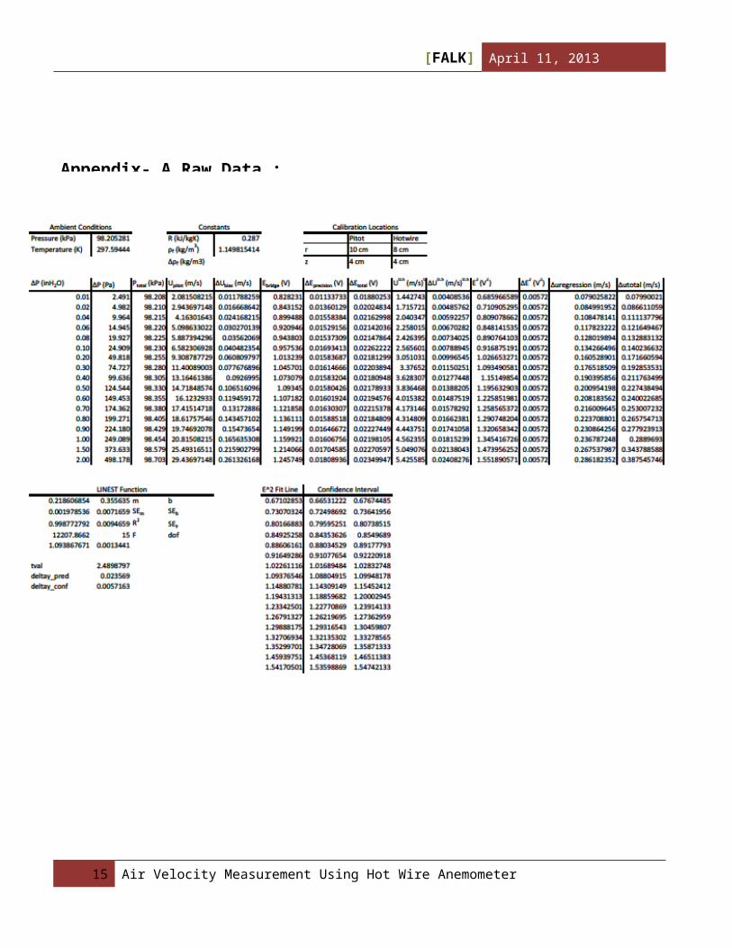
Appendix- A Raw Data :


[ ] April 11, 2013


[ ] April 11, 2013

z r r/r_20% E SE SU U u'/U

8 1.2 60.96551

10.06843

51.65134

4 11.2001 0.14744

8 1 51.04963

4 0.06422.00462

2 11.20010.17898

3

8 0.8 41.09093

70.05210

91.81989

4 11.20010.16248

9

8 0.6 31.15527

40.04470

81.83181

1 11.20010.16355

3

8 0.4 21.22336

90.03397

41.62230

9 11.20010.14484

8

8 0.2 11.23824

40.02921

81.43997

7 11.20010.12856

8

8 0 01.24331

1 0.028141.40165

7 11.20010.12514

7

18 2.5 5 0.86550.06510

81.07209

25.89985

40.18171

5

18 2 40.92761

80.06205

3 1.311055.89985

40.22221

7

18 1.5 30.99409

80.04897

51.29659

25.89985

40.21976

7

18 1 21.03668

80.05255

51.58160

55.89985

40.26807

5

18 0.5 11.08539

30.04009

41.38002

75.89985

40.23390

9

18 0 01.10429

10.03497

51.26440

25.89985

40.21431

1

28 3.95.57142

90.80928

80.06788

70.85038

13.78164

30.22487

1

28 3.14.42857

10.86384

60.05923

30.96826

23.78164

30.25604

3

28 2.33.28571

40.92085

50.04583

10.94433

53.78164

30.24971

5

28 1.52.14285

70.96916

20.05724

31.39820

23.78164

30.36973

4

28 0.7 10.99272

90.04228

81.11474

33.78164

30.29477

7

28 0 01.02333

70.03182

80.92120

53.78164

30.24359

9


[ ] April 11, 2013

38 5.74.38461

50.74381

10.03336

90.27597

92.56419

50.10762

8

38 4.63.53846

20.76559

40.02792

4 0.269372.56419

50.10505

1

38 3.52.69230

80.89679

90.03157

30.59277

62.56419

50.23117

4

38 2.41.84615

4 0.89961 0.048420.91930

72.56419

50.35851

7

38 1.3 10.97555

90.03007

30.75021

22.56419

50.29257

2

38 0 0 0.961830.03742

80.89202

92.56419

50.34787

9


Documents

Air Velocity Anemometer Lab