Embed Size (px)
Citation preview

Master’s ThesisMàster Universitari en Enginyeria de l’Energia (MUEE)
Air Turbine Rotational Speed Control ofOscillating-Water-Column Wave Energy
Converters
DISSERTATIONOctober 28, 2020
Author: Francisco Serejo Soares Branco
Director: Josep Bordonau Farrerons
Call:
Escola Tècnica Superiord’Enginyeria Industrial de Barcelona

Page ii Dissertation

Air Turbine Rotational Speed Control of Oscillating-Water-Column Wave Energy Converters Page iii
Preamble
The Coronavirus disease 2019 pandemic occurred simultaneously with the development of the present
work and led to the closure of all testing facilities in the faculty where this work was originally set to
take place: Instituto Superior Técnico, located in Lisbon, Portugal. The dissertation’s planning initially
predicted the experimental testing of an oscillating-water-column wave energy converter model in the
faculty’s wave tank. Due to its closure, the dissertation’s planning had to be altered: the chosen alterna-
tive was to develop a project in the same scientific field, but focused on numerical simulations.
The initially planned experiments are described in annex A.

Page iv Dissertation

Air Turbine Rotational Speed Control of Oscillating-Water-Column Wave Energy Converters Page v
Abstract
The air turbine rotational speed control of oscillating-water-column wave energy converters is addressed.
A wave energy converter is a device which is able to extract energy from the incident waves. In an
oscillating-water-column, the predominant wave energy converter design, an air turbine is driven by the
compression and decompression of air inside a chamber, originated by the motion of incident waves.
Interactions between the incident waves and an oscillating-water-column wave energy converter are stud-
ied under the uniform pressure model and linear wave theory. In the uniform pressure model, the radia-
tion flow rate, i.e., the flow rate of air caused solely by the air pressure oscillation inside the chamber, is
a strongly non-linear effect. Its analytical calculation represents an extremely demanding computational
task and, therefore, it must be modelled through a faster alternative method: Prony’s method.
A techno-economic comparative analysis is performed between the self-rectifying Wells turbine, tradi-
tionally utilized in oscillating-water-column wave energy converters, and the novel self-rectifying bi-
radial impulse turbine. The comparative work is carried out for the case study of the Pico wave power
plant: a fixed structure oscillating-water-column wave energy converter which represents one of the
largest wave energy technology research and development hubs ever conceived.
The technical and economic results obtained for the case study plant serve as a general representation of
the current wave energy technology framework. More specifically, they do so regarding the fixed struc-
ture oscillating-water-column, one of the most currently developed wave energy converter designs.
The present work’s fundamental purpose is to develop the numerical model of the Pico wave power plant.
This work also encompasses several additional objectives, being the most relevant:
• Validation of the radiation flow rate’s modelling through Prony’s method.
• Implementation of air turbine rotational speed control in an oscillating-water-column wave energy
converter operating with the Wells and bi-radial turbines and comparison of the obtained results.
• Turbine diameter optimization for electrical energy production maximization and profit maximiza-
tion under various potential economic scenarios.
The selected radiation flow rate model, acquired through Prony’s method, was satisfactory in terms of
accuracy and computational speed. It demonstrated very acceptable error metrics for nearly all wave
frequencies encountered in real environment conditions.
In an oscillating-water-column wave energy converter under real environment conditions, it was exper-
imentally verified that the bi-radial turbine, partially due to its lower rotational speed, demonstrates a
superior energy extraction relatively to the Wells turbine. The energy extraction of the bi-radial turbine
was also found to be strongly constrained by the rated power of the coupled electrical generator.
Finally, the turbine diameter optimization results for profit maximization indicate that wave energy tech-
nology is not yet prepared for full-scale implementation, unless financial support is readily made avail-
able. Nevertheless, the almost positive return on investment for some of the potential economic scenarios
tested and the technology’s operational profitability, verified for all cases, are extremely encouraging.
Currently, the high construction cost and low electricity selling price are two key economic barriers to
further development of wave energy technology. The solution to these barriers may respectively be the
incorporation of oscillating-water-column wave energy converters in a breakwater (an alternative already
proposed by several authors) and the implementation of favorable governmental policies regarding wave
energy technology, such as tax benefits or public fixed subsidies for the electricity selling price.

Page vi Dissertation

Air Turbine Rotational Speed Control of Oscillating-Water-Column Wave Energy Converters Page vii
Contents
1 Introduction 1
1.1 Motivation . . . . . . . . . . . . . . . . . . . . . . . . . . . . . . . . . . . . . . . . . . 1
1.2 Problem Formulation . . . . . . . . . . . . . . . . . . . . . . . . . . . . . . . . . . . . 2
1.3 Contribution . . . . . . . . . . . . . . . . . . . . . . . . . . . . . . . . . . . . . . . . . 3
1.4 Thesis Outline . . . . . . . . . . . . . . . . . . . . . . . . . . . . . . . . . . . . . . . . 3
2 State-of-the-Art 6
2.1 Wave Energy Converters . . . . . . . . . . . . . . . . . . . . . . . . . . . . . . . . . . 6
2.2 Air Turbines . . . . . . . . . . . . . . . . . . . . . . . . . . . . . . . . . . . . . . . . . 8
2.3 Air Turbine Rotational Speed Control . . . . . . . . . . . . . . . . . . . . . . . . . . . 9
3 Linear Wave Theory 12
3.1 Fundamental Equations . . . . . . . . . . . . . . . . . . . . . . . . . . . . . . . . . . . 12
3.2 Regular Waves . . . . . . . . . . . . . . . . . . . . . . . . . . . . . . . . . . . . . . . 14
3.2.1 Wave Energy and Power . . . . . . . . . . . . . . . . . . . . . . . . . . . . . . 16
3.3 Irregular Waves . . . . . . . . . . . . . . . . . . . . . . . . . . . . . . . . . . . . . . . 17
3.3.1 Variance Density and Energy Density Spectra . . . . . . . . . . . . . . . . . . . 17
3.3.2 Representative Parameters of Irregular Waves . . . . . . . . . . . . . . . . . . . 19
3.3.3 Wave Power . . . . . . . . . . . . . . . . . . . . . . . . . . . . . . . . . . . . . 19
4 Uniform Pressure Modelling of Oscillating-Water-Column Wave Energy Converters 21
4.1 Uniform Pressure Model Formulation . . . . . . . . . . . . . . . . . . . . . . . . . . . 21
4.2 Frequency Domain Analysis . . . . . . . . . . . . . . . . . . . . . . . . . . . . . . . . 23
4.3 Time Domain Analysis . . . . . . . . . . . . . . . . . . . . . . . . . . . . . . . . . . . 25
4.3.1 Time Domain Analysis Formulation . . . . . . . . . . . . . . . . . . . . . . . . 25
4.3.2 Classic Runge-Kutta Method . . . . . . . . . . . . . . . . . . . . . . . . . . . . 27

Page viii Dissertation
4.3.3 Prony’s Method . . . . . . . . . . . . . . . . . . . . . . . . . . . . . . . . . . . 28
5 Air Turbine Rotational Speed Control 32
5.1 Rotational Speed Control Formulation . . . . . . . . . . . . . . . . . . . . . . . . . . . 32
5.2 Turbine Diameter Optimization . . . . . . . . . . . . . . . . . . . . . . . . . . . . . . . 34
5.2.1 Electrical Energy Production Maximization . . . . . . . . . . . . . . . . . . . . 35
5.2.2 Profit Maximization . . . . . . . . . . . . . . . . . . . . . . . . . . . . . . . . 35
6 Experiments and Results — Pico Plant Case Study 39
6.1 Experimental Data . . . . . . . . . . . . . . . . . . . . . . . . . . . . . . . . . . . . . 39
6.1.1 Hydrodynamics, Wave Climate and Structure . . . . . . . . . . . . . . . . . . . 39
6.1.2 Turbine-Generator Systems . . . . . . . . . . . . . . . . . . . . . . . . . . . . 40
6.1.3 Economic Description . . . . . . . . . . . . . . . . . . . . . . . . . . . . . . . 42
6.2 Frequency Domain Analysis . . . . . . . . . . . . . . . . . . . . . . . . . . . . . . . . 43
6.3 Radiation Flow Rate Modelling through Prony’s Method . . . . . . . . . . . . . . . . . 44
6.4 Time Domain Analysis — Rotational Speed Control under Irregular Waves . . . . . . . 48
6.5 Turbine Diameter Optimization . . . . . . . . . . . . . . . . . . . . . . . . . . . . . . . 52
6.5.1 Electrical Energy Production Maximization . . . . . . . . . . . . . . . . . . . . 52
6.5.2 Profit Maximization . . . . . . . . . . . . . . . . . . . . . . . . . . . . . . . . 53
6.5.3 Optimized Results . . . . . . . . . . . . . . . . . . . . . . . . . . . . . . . . . 59
7 Preliminary Planning and Costs — Pico Plant Case Study 63
7.1 Project Planning . . . . . . . . . . . . . . . . . . . . . . . . . . . . . . . . . . . . . . . 63
7.2 Cost Analysis . . . . . . . . . . . . . . . . . . . . . . . . . . . . . . . . . . . . . . . . 63
8 Environmental Impact — Pico Plant Case Study 66
8.1 Avoided Emissions . . . . . . . . . . . . . . . . . . . . . . . . . . . . . . . . . . . . . 66
8.2 Socioeconomic Impact . . . . . . . . . . . . . . . . . . . . . . . . . . . . . . . . . . . 66

Air Turbine Rotational Speed Control of Oscillating-Water-Column Wave Energy Converters Page ix
9 Conclusions 68
10 Appreciations 71
A Initial Experiments 77
B Wave Energy Theory 81
B.1 Modes of Oscillation of a Body . . . . . . . . . . . . . . . . . . . . . . . . . . . . . . . 81
B.2 Linearization of the Pressure and Kinematic Boundary Conditions . . . . . . . . . . . . 81
B.3 Derivation of the Velocity Potential of Regular Waves . . . . . . . . . . . . . . . . . . . 82
B.4 Ideal Gas Isentropic Thermodynamics . . . . . . . . . . . . . . . . . . . . . . . . . . . 83
C Experiments and Results 86
C.1 Wave Climate . . . . . . . . . . . . . . . . . . . . . . . . . . . . . . . . . . . . . . . . 86
C.2 Cost Calculation . . . . . . . . . . . . . . . . . . . . . . . . . . . . . . . . . . . . . . . 87
C.3 Frequency Domain Analysis — Linearized Bi-radial Turbine . . . . . . . . . . . . . . . 88
C.4 Prony’s Method Tested Cases . . . . . . . . . . . . . . . . . . . . . . . . . . . . . . . . 90
C.5 Radiation Flow Rate Modelling — Levy Identification Method vs Prony’s Method . . . . 92

Page x Dissertation

Air Turbine Rotational Speed Control of Oscillating-Water-Column Wave Energy Converters Page xi
List of Figures
1.1 Illustration of the energy pathways in wave energy technology, adapted from [5]. . . . . 1
1.2 Later construction stages of the Pico plant (1998): rear view (top left), front view (top
right) and turbine room before turbine assembly (bottom). Adapted from [8]. . . . . . . 2
2.1 WEC design examples: fixed structure overtopping (top), floating OWC (bottom left)
and heave submerged oscillating body (bottom right). Adapted from [9] and [12]. . . . . 6
2.2 Illustration of the WEC design working principle categorization, adapted from [4]. . . . 7
2.3 Illustration of the fixed structure (left) and floating (right) OWC WEC designs, adapted
from [4] and [9]. . . . . . . . . . . . . . . . . . . . . . . . . . . . . . . . . . . . . . . 8
2.4 Illustration of the axial-flow Wells (left) and bi-radial impulse (right) turbines, adapted
from [9]. . . . . . . . . . . . . . . . . . . . . . . . . . . . . . . . . . . . . . . . . . . . 9
3.1 Illustration of the disturbed water free surface vertical displacement of a regular wave. . 15
3.2 Illustration of variance density spectra and corresponding wave records, adapted from [12]. 18
4.1 Illustration of the oscillating body (left) and uniform pressure (right) models, adapted
from [12]. . . . . . . . . . . . . . . . . . . . . . . . . . . . . . . . . . . . . . . . . . . 21
4.2 Illustration of the classic Runge-Kutta method, adapted from [27]. . . . . . . . . . . . . 27
5.1 Illustration of the Wells-adapted rotational speed control law, adapted from [14]. . . . . . 34
6.1 Pico plant’s hydrodynamic coefficients: radiation conductance, radiation susceptance
and excitation flow rate coefficient. . . . . . . . . . . . . . . . . . . . . . . . . . . . . . 39
6.2 Turbine performance dimensionless coefficients: Pico plant’s original Wells turbine. . . . 41
6.3 Turbine performance dimensionless coefficients: bi-radial turbine. . . . . . . . . . . . . 42
6.4 Results for the frequency domain analysis of the Pico plant operating with the original
Wells turbine: complex amplitudes of the excitation flow rate (top left), air pressure
oscillation inside the chamber (top right) and radiation flow rate (bottom left); time-
averaged pneumatic power available to the turbine (bottom right). . . . . . . . . . . . . 44
6.5 Relative root-mean-square error of the pneumatic power available to the turbine for the
Pico plant operating with the original Wells turbine: total (top) and real environment
(bottom) wave frequency range. . . . . . . . . . . . . . . . . . . . . . . . . . . . . . . 46
6.6 Correlation coefficient of the pneumatic power available to the turbine for the Pico plant
operating with the original Wells turbine: total (top) and real environment (bottom) wave
frequency range. . . . . . . . . . . . . . . . . . . . . . . . . . . . . . . . . . . . . . . 47

Page xii Dissertation
6.7 Memory function: analytical computation and Prony’s method approximations. . . . . . 48
6.8 Annual time-averaged electrical power supplied to the grid for the Pico plant operating
with distinct turbine-generator systems. . . . . . . . . . . . . . . . . . . . . . . . . . . 52
6.9 Utilization factor for the Pico plant operating with distinct turbine-generator systems. . . 52
6.10 Net present value for the Pico plant operating with distinct turbine-generator systems and
electricity selling price scenarios (solid lines for u = 0.225AC/kWh and dashed lines for
u = 0.047AC/kWh). . . . . . . . . . . . . . . . . . . . . . . . . . . . . . . . . . . . . . 53
6.11 Net present value for the Pico plant operating with distinct turbine-generator systems and
discount rate scenarios (solid lines for r = 5% and dashed lines for r = 15%). . . . . . . 54
6.12 Net present value for the Pico plant operating with distinct turbine-generator systems
and mechanical equipment cost metric scenarios (solid lines for Bmech = 25kAC/m2 and
dashed lines for Bmech = 78kAC/m2). . . . . . . . . . . . . . . . . . . . . . . . . . . . . 55
6.13 Net present value for the Pico plant operating with distinct turbine-generator systems and
electrical equipment cost metric scenarios (solid lines for Belec = 2.5kAC/m0.7 and dashed
lines for Belec = 4.2kAC/m0.7). . . . . . . . . . . . . . . . . . . . . . . . . . . . . . . . 55
6.14 Net present value for the Pico plant operating with distinct turbine-generator systems
and construction cost scenarios (solid lines for Cstruc = 1667kAC and dashed lines for
Cstruc = 5001kAC). . . . . . . . . . . . . . . . . . . . . . . . . . . . . . . . . . . . . . 56
6.15 Net present value for the Pico plant operating with distinct turbine-generator systems in
the best scenario. . . . . . . . . . . . . . . . . . . . . . . . . . . . . . . . . . . . . . . 57
6.16 Net present value for the Pico plant operating with distinct turbine-generator systems in
the worst scenario. . . . . . . . . . . . . . . . . . . . . . . . . . . . . . . . . . . . . . 58
6.17 Net present value for the Pico plant operating with distinct turbine-generator systems in
the average scenario. . . . . . . . . . . . . . . . . . . . . . . . . . . . . . . . . . . . . 58
6.18 Time-averaged turbine efficiency for the Pico plant operating with the diameter opti-
mized turbine-generator systems. . . . . . . . . . . . . . . . . . . . . . . . . . . . . . . 60
6.19 Time-averaged turbine rotational speed for the Pico plant operating with the diameter
optimized constrained and unconstrained turbine-generator systems. . . . . . . . . . . . 60
7.1 Gantt chart from the start of conceptualization to the end of civil construction for the
development of the present day Pico plant. . . . . . . . . . . . . . . . . . . . . . . . . . 63
A.1 OWC WEC model preliminary technical drawing (measurements in millimeters). . . . . 77

Air Turbine Rotational Speed Control of Oscillating-Water-Column Wave Energy Converters Page xiii
A.2 OWC WEC model with fixed support: three-quarter view (left), tube top opening detail
(top right) and tube adjustment mechanism detail (bottom right). . . . . . . . . . . . . . 78
A.3 Illustration of the latching control system, adapted from [40]. . . . . . . . . . . . . . . . 79
A.4 Latching control system: top view (left), camera’s original control board detail (top right)
and camera’s diaphragm detail (bottom right). . . . . . . . . . . . . . . . . . . . . . . . 79
B.1 Illustration of the six modes of oscillation of a body. . . . . . . . . . . . . . . . . . . . . 81
C.1 Variance density spectra for the condensed Pico plant’s wave climate. . . . . . . . . . . 86
C.2 All available Portuguese historical inflation rates from 1996 to 2020, adapted from [43]. . 88
C.3 Dimensionless flow rate vs dimensionless pressure head experimental curve and respec-
tive linear fit for the bi-radial turbine. . . . . . . . . . . . . . . . . . . . . . . . . . . . . 89
C.4 Results for the frequency domain analysis of the Pico plant operating with the linearized
bi-radial turbine: complex amplitudes of the excitation flow rate (top left), air pressure
oscillation inside the chamber (top right) and radiation flow rate (bottom left); time-
averaged pneumatic power available to the turbine (bottom right). . . . . . . . . . . . . 89
C.5 Modelling of the Pico plant operating with the original Wells turbine through the Levy
identification method: model gain, phase and roots’ placement. . . . . . . . . . . . . . . 93
C.6 Relative root-mean-square error of the pneumatic power available to the turbine for the
Pico plant operating with the original Wells turbine: total (top) and real environment
(bottom) wave frequency range. Comparison between all tested radiation flow rate mod-
elling methods. . . . . . . . . . . . . . . . . . . . . . . . . . . . . . . . . . . . . . . . 94
C.7 Correlation coefficient of the pneumatic power available to the turbine for the Pico plant
operating with the original Wells turbine: total (top) and real environment (bottom) wave
frequency range. Comparison between all tested radiation flow rate modelling methods. . 95
C.8 Modelling of the Pico plant operating with the linearized bi-radial turbine through the
Levy identification method: model gain, phase and roots’ placement. . . . . . . . . . . . 96
C.9 Relative root-mean-square error (top) and correlation coefficient (bottom) of the pneu-
matic power available to the turbine for the Pico plant operating with the linearized bi-
radial turbine in the real environment wave frequency range. Comparison between all
tested radiation flow rate modelling approximation methods. . . . . . . . . . . . . . . . 97

Page xiv Dissertation

Air Turbine Rotational Speed Control of Oscillating-Water-Column Wave Energy Converters Page xv
List of Tables
6.1 Pico plant’s condensed wave climate data. . . . . . . . . . . . . . . . . . . . . . . . . . 40
6.2 Turbine-generator system technical description: Pico plant’s original Wells turbine (mid-
dle column) and bi-radial turbine (right column). . . . . . . . . . . . . . . . . . . . . . 41
6.3 Turbine-generator system economic description: possible economic scenarios. . . . . . . 42
6.4 Time-averaged electrical power supplied to the grid vs turbine diameter for the Pico plant
operating with the original Wells turbine and the original electrical generator. . . . . . . 50
6.5 Time-averaged electrical power supplied to the grid vs turbine diameter for the Pico plant
operating with the bi-radial turbine and the original electrical generator. . . . . . . . . . 50
6.6 Time-averaged electrical power supplied to the grid vs turbine diameter for the Pico plant
operating with the bi-radial turbine and the 600kW electrical generator. . . . . . . . . . 51
6.7 Time-averaged electrical power supplied to the grid vs turbine diameter for the Pico plant
operating with the bi-radial turbine and the 800kW electrical generator. . . . . . . . . . 51
6.8 Diameter optimized results for the Pico plant operating with distinct turbine-generator
systems, regarding electrical energy production maximization. . . . . . . . . . . . . . . 53
6.9 Break-even electricity selling price for the Pico plant operating with distinct turbine-
generator systems. . . . . . . . . . . . . . . . . . . . . . . . . . . . . . . . . . . . . . . 54
6.10 Internal rate of return for the Pico plant operating with distinct turbine-generator systems. 54
6.11 Break-even construction cost for the Pico plant operating with distinct turbine-generator
systems. . . . . . . . . . . . . . . . . . . . . . . . . . . . . . . . . . . . . . . . . . . . 56
6.12 Net present value, internal rate of return and payback period for the Pico plant operating
with distinct turbine-generator systems in the best scenario. . . . . . . . . . . . . . . . . 57
6.13 Net present value and internal rate of return for the Pico plant operating with distinct
turbine-generator systems in the worst scenario. . . . . . . . . . . . . . . . . . . . . . . 58
6.14 Net present value and internal rate of return for the Pico plant operating with distinct
turbine-generator systems in the average scenario. . . . . . . . . . . . . . . . . . . . . . 59
7.1 Capital costs of the Pico plant operating with the bi-radial turbine and the 800kW elec-
trical generator in the average scenario. . . . . . . . . . . . . . . . . . . . . . . . . . . 64
7.2 Annual operational cost of the Pico plant operating with the bi-radial turbine and the
800kW electrical generator in the average scenario. . . . . . . . . . . . . . . . . . . . . 64
C.1 Pico plant’s complete wave climate data. . . . . . . . . . . . . . . . . . . . . . . . . . . 87

Page xvi Dissertation
C.2 Prony’s method for np = 10 complex negative exponential functions: initial amplitude,
initial phase, damping factor and temporal frequency. . . . . . . . . . . . . . . . . . . . 90
C.3 Prony’s method for np = 10 complex negative exponential functions: time-dependent
and independent parts of the memory function approximation. . . . . . . . . . . . . . . 90
C.4 Prony’s method for np = 15 complex negative exponentials functions: initial amplitude,
initial phase, damping factor and temporal frequency. . . . . . . . . . . . . . . . . . . . 91
C.5 Prony’s method for np = 15 complex negative exponentials functions: time-dependent
and independent parts of the memory function approximation. . . . . . . . . . . . . . . 91
C.6 Modelling of the Pico plant operating with the original Wells turbine through the Levy
identification method: model denominator and numerator. . . . . . . . . . . . . . . . . . 94
C.7 Modelling of the Pico plant operating with the linearized bi-radial turbine through the
Levy identification method: model denominator and numerator. . . . . . . . . . . . . . 96

Air Turbine Rotational Speed Control of Oscillating-Water-Column Wave Energy Converters Page xvii

Page xviii Dissertation
List of Acronyms
WEC Wave Energy Converter
PTO Power Take-Off
R&D Research and Development
OWC Oscillating-Water-Column
O&M Operation and Management
WRIG Wound Rotor Induction Generator

Air Turbine Rotational Speed Control of Oscillating-Water-Column Wave Energy Converters Page xix

Page xx Dissertation
List of Symbols
Romans
A regulation curve coefficient for the Wells-adapted control law [W/s]Aw wave amplitude [m]abepref
reference rotational speed control parameter at the best efficiency point [W·s3]Belec electrical equipment cost metric [kAC/W0.7]Bmech mechanical equipment cost metric [kAC/m3X ]Cstruc construction cost [kAC]CWRctrl electrical capture width ratio [-]D turbine diameter [m]Dref reference turbine diameter [m]fav fractional availability [-]G radiation conductance [m4·s/kg]g gravitational acceleration [m/s2]H radiation susceptance [m4·s/kg]Hs significant wave height [m]h water bed depth [m]hr memory function [m3/s2·Pa]Iref reference moment of inertia of the rotating parts [kg·m2]IRR internal rate of return [%]i imaginary unitK turbine geometry constant [-]k wave number [rad/m]l chamber length [m]Nw number of regular waves forming an irregular wave [-]NPV net present value [kAC]n project’s lifetime [year]np Prony’s method number of complex negative exponential functions [-]Pc complex amplitude of the air pressure oscillation inside the chamber [Pa]Pctrl electrical power supplied to the grid [kW]Pctrl time-averaged electrical power supplied to the grid [kW]Pctrla annual time-averaged electrical power supplied to the grid [kW]Prated
gen generator rated power [kW]Pmax turbine power output limit for the Wells-adapted control law [kW]Ppneu pneumatic power available to the turbine [kW]Ppneu time-averaged pneumatic power available to the turbine [kW]Pt turbine power output [kW]Pwave wave power [kW/m]Pwavea annual wave power [kW/m]PBP payback period [year]pa atmospheric pressure [Pa]pc air pressure oscillation inside the chamber [Pa]Qe complex amplitude of the excitation flow rate [m3/s]Qr complex amplitude of the radiation flow rate [m3/s]qe excitation flow rate [m3/s]

Air Turbine Rotational Speed Control of Oscillating-Water-Column Wave Energy Converters Page xxi
qr radiation flow rate [m3/s]Rpneu correlation coefficient of the pneumatic power available to the turbine [-]RRMSEpneu relative root-mean-square error of the pneumatic power available to the turbine [%]r discount rate [%]ri inflation rate [%]Sω variance density spectrum for wave frequency [m2·s/rad]T wave period [s]Tctrl imposed electromagnetic torque from the generator to the turbine shaft [N·m]Te energy period [s]Ts computational time step [s]t continuous time [s]u electricity selling price [AC/kWh]Vc air volume inside the chamber [m3]Vc0 air volume inside the chamber in the absence of incident waves [m3]w chamber width [m]X economy of scale exponent [-]
Greek Symbols
α wave phase angle [rad]αf utilization factor [-]αpc phase of the air pressure oscillation inside the chamber [rad]αqe phase of the excitation flow rate [rad]αqr phase of the radiation flow rate [rad]Γ excitation flow rate coefficient [m2/s]γ air specific heat ratio [-]ζ disturbed water free surface vertical displacement [m]η turbine efficiency [-]η time-averaged turbine efficiency [-]λ wavelength [m]Π dimensionless coefficient of power output [-]ρa atmospheric density [kg/m3]Φ dimensionless coefficient of flow rate [-]φ water particle velocity potential [m2/s]φs sea state probability of occurrence [%]ϕ amplitude of the water particle velocity potential [m2/s]Ψ dimensionless coefficient of pressure head [-]Ω turbine rotational speed [rad/s]Ω time-averaged turbine rotational speed [rad/s]Ωmax
gen generator rotational speed limit [rad/s]Ωmax turbine-generator system rotational speed limit [rad/s]ω wave frequency [rad/s]ωe energy wave frequency [rad/s]ωs computational wave frequency step [rad/s]

Page xxii Dissertation

Air Turbine Rotational Speed Control of Oscillating-Water-Column Wave Energy Converters Page 1
1 Introduction
Wave energy is one of the most disregarded energy generation sources in the current renewable energy
supply mix. In spite of that, the global wave energy resource is extremely significant, being estimated at
50.64±1.20TWh/dayfor 95% confidence intervals [1].
Assessing the global wave power resource, the large availability in Western European coast locations
is particularly significant. This is the case of Portugal and Spain, where the wave power ranges from
5.42kW/m to 58.48kW/m [2] (note that the wave power density is commonly referred to as wave power).
Additionally, the large wave power resource and low seasonality in energetically underdeveloped regions
such as Western Africa and South America is very encouraging, while the combination of wave energy
and offshore wind energy technologies is an evident possibility with substantial potential [3].
Unlike more mature renewable energy generation technologies, there is not a predominant design in wave
energy technology [4]. Several distinct physical principles for wave energy extraction have arisen and
resulted in a multitude of designs for a Wave Energy Converter (WEC). A review of the currently most
relevant WEC designs is presented in section 2.1.
A WEC is a device able to extract energy from incident waves using a Power Take-Off (PTO) mechanism.
A PTO mechanism enables the conversion of the energy from incident waves into other forms of energy
(for example, mechanical or electrical).
The operation of a specific PTO mechanism is directly linked with the WEC design. Currently, the main
PTO mechanisms are air turbines, hydro turbines, hydraulic circuits, direct mechanical drive systems,
electrical generators and direct electrical drive systems [5]. The most common energy pathways in wave
energy technology are illustrated in figure 1.1.
Figure 1.1: Illustration of the energy pathways in wave energy technology, adapted from [5].
1.1 Motivation
In 1992-1993, the European Commission initiated the European Pilot Plant Study, in order to find a
suitable location for a wave energy pilot plant. The chosen location was Porto Cachorro, in the island of
Pico, Azores, Portugal (northern Atlantic Ocean). After preliminary studies, the construction of the Pico
wave power plant, or simply Pico plant, was launched in 1996 [6].

Page 2 Dissertation
The Pico plant served as a Research and Development (R&D) facility for full scale testing of newly
developed air turbines. Additionally, it helped supply the electrical grid of the island.
The plant was assembled on the natural rocky bottom of a gully in Porto Cachorro’s coastline. Its PTO
mechanism consisted in the combination of an air turbine with an electrical generator.
Construction ended by 1998, but the first full scale tests were postponed to 1999 due to flooding and
malfunction accidents [7]. Additional malfunctions hindered the plant’s operation in the following years.
In 2004, the Wave Energy Centre, a non-profit organization that focuses on wave energy (now renamed
Wave Energy Centre Offshore Renewables), began the restoration of the plant: it was operational by
2005. After more than a decade in operation, the Pico plant would ultimately be closed due to its partial
collapse under stormy conditions, in April of 2018 [6].
Despite its closure, the Pico plant has been one of the main R&D hubs for wave energy technology
throughout more than a decade. It has greatly contributed to innovation in this scientific field, being
featured in over a hundred scientific publications. Still today, as this work is an example of, the Pico
plant serves as a case study regarding the technical and economic feasibility of wave energy technology.
Figure 1.2 illustrates the later stages of the Pico plant’s construction in 1998.
Figure 1.2: Later construction stages of the Pico plant (1998): rear view (top left), front view (top right)and turbine room before turbine assembly (bottom). Adapted from [8].
1.2 Problem Formulation
Nowadays, the Oscillating-Water-Column (OWC) is generally considered the simplest, most reliable and
most researched WEC design [9]. It is the subject of the present work.
The OWC WEC, further explained in section 2.1, consists of an air chamber with its bottom surface open
under the mean water level and connected to the outer atmosphere through an air turbine. The action of
the incident waves generates a water column that moves relatively to the air inside the chamber. The
resulting air pressure difference drives a turbine which, in turn, feeds an electrical generator.
The aerodynamic performance of the air turbine is fundamental to the wave energy extraction of an OWC
WEC [10]. In real environment conditions, waves are extremely irregular. As a result, converting the
energy of the incident waves while maintaining a constant turbine rotational speed is an ineffective strat-
egy. To ensure the wave energy extraction is suitably performed, the rotational speed of the turbine must
be controlled.

Air Turbine Rotational Speed Control of Oscillating-Water-Column Wave Energy Converters Page 3
Rotational speed control consists in affecting the efficiency of an air turbine through the regulation of
its rotational speed, using a programmable logic controller. This form of control is usually performed
through the torque applied by the electrical generator on the turbine [11].
Lastly, the air turbine diameter is one of the essential design parameters of an OWC WEC. To attain
optimal results, a turbine diameter optimization is required. There are two turbine diameter optimization
criteria: maximization of the electrical energy production and maximization of the project’s profit.
Ultimately, the turbine rotational speed control and diameter optimization results depend on the studied
location’s wave climate, the OWC WEC’s hydrodynamics, the turbine aerodynamic performance, the ro-
tational speed control and the project’s economic description. All these components must be extensively
modelled, including the non-linear effect for the flow rate inside the OWC WEC’s chamber.
1.3 Contribution
First, this work outlines the dominant WEC and air turbine designs in wave energy technology.
Furthermore, the present work features a general overview of linear wave theory, the prevailing theoret-
ical basis of wave energy technology, and submits a summary for the uniform pressure modelling of an
OWC WEC. Thus, it can serve as an introduction to wave energy theory for uninformed readers.
A synopsis of rotational speed control theory applied to OWC WECs is developed. Both the traditional
Wells and the novel impulse turbine designs are considered.
This work also contributes with an extensive description of its case study: the Pico plant. It serves as
a compilation of numerous scientific articles regarding the history, structure, hydrodynamics, wave cli-
mate, PTO mechanisms, technical analysis and economic analysis of the Pico wave power plant.
An additional contribution is the testing of Prony’s method for the modelling of the radiation flow rate.
This method is relatively new in the literature concerning this particular application.
Finally, the present work contributes with the rotational speed control and subsequent turbine diame-
ter optimization for the Pico plant. A comparative analysis is performed between the Wells turbine,
extensively recorded in the literature, and the more recent bi-radial impulse turbine. The results and
conclusions from the case study help generally establish the techno-economic key drivers and barriers to
the future development of wave energy technology.
1.4 Thesis Outline
In section 2, a summary of the predominant WEC and air turbine designs in wave energy technology is
given. Also, the rotational speed control of a turbine in an OWC WEC is briefly described.
Section 3 provides a comprehensive description of linear wave theory. The action of both regular and
irregular waves is modelled for distinct cases of the water bed depth.
The dynamics of an OWC WEC are modelled according to the uniform pressure model, in section 4.
The main equations for the frequency domain and time domain analyses are defined. Additionally, the
theoretical basis for the modelling of the radiation flow rate through Prony’s method is presented.
Section 5 describes turbine rotational speed control in an OWC WEC. Furthermore, turbine diameter
optimization is studied for the maximization of both electrical energy production and profit. The latter
implied the creation of an economic model for the construction and operation of the OWC WEC.
In section 6, the case study of the Pico wave power plant is presented. In this section are the technical
and economic descriptions of the plant and of the tested PTO mechanisms, as well as the procedures and

Page 4 Dissertation
results for all performed experiments. The performed experiments were: frequency domain analysis,
modelling of the radiation flow rate through Prony’s method, rotational speed control of the tested PTO
mechanisms in real environment conditions and turbine diameter optimization for maximum electrical
energy production and profit maximization. Regarding the latter, the effect of each economic component
in the final profitability of the project was additionally tested through sensitivity analyses.
Annex A describes the initially performed experiments before the alteration in the dissertation’s planning.
Annex B reviews basic concepts necessary to derive the equations in sections 3 and 4.
Annex C contains additional experiments and results regarding the Pico plant’s wave climate, economic
description, frequency domain analysis and modelling of the radiation flow rate, either through Prony’s
method or Levy identification method.

Air Turbine Rotational Speed Control of Oscillating-Water-Column Wave Energy Converters Page 5

Page 6 Dissertation
2 State-of-the-Art
The first ever WEC patent was filed in Paris, France, in 1799. More than one century later, modern wave
energy technology began with the development of the pioneering OWC WEC, created by Yoshio Masuda
in the 1940’s.
It was only by 1975 that wave energy technology attracted significant attention, when the British Govern-
ment created a nationwide R&D program focused on several WEC designs. Meanwhile, in the 1980’s,
Johannes Falnes and David Evans greatly developed the theoretical and experimental basis of wave
energy conversion. By 1982, the failure of the British Government’s program meant that a similar in-
vestment would only appear in the next decade when, in 1992, the European Commission’s first wave
energy projects were introduced.
From the 1990’s to the present day, the European Commission has funded numerous projects regarding
wave energy technology R&D (wave energy resource assessment, air turbine optimization, WEC design
development, etc.), placing Europe in the vanguard of this scientific field [12].
2.1 Wave Energy Converters
Currently, the physical principle for wave energy extraction of most WEC designs is based on the os-
cillation of a water column or a rigid body. It is relevant to recall that a body is allowed six modes of
oscillation: heave, surge, sway, yaw, roll and pitch. These are illustrated in figure B.1.
WEC designs can be categorized according to various criteria. Currently, the most common approach
is to categorize WEC designs by working principle. This results in three main categories: overtopping,
oscillating body and OWC.
Examples of WEC designs are presented in figure 2.1.
Figure 2.1: WEC design examples: fixed structure overtopping (top), floating OWC (bottom left) andheave submerged oscillating body (bottom right). Adapted from [9] and [12].

Air Turbine Rotational Speed Control of Oscillating-Water-Column Wave Energy Converters Page 7
Figure 2.2 illustrates the working principle categorization.
Figure 2.2: Illustration of the WEC design working principle categorization, adapted from [4].
In the overtopping design, the water of incident waves is stored by reservoirs placed above the mean
water level. Then, through water turbines, the potential energy of the incident waves is converted into
mechanical energy, which in turn feeds an electrical generator. Overtopping WECs can be floating or
fixed structures. In the latter case, the WEC can be installed either at the shoreline or in a breakwater.
A breakwater is a structure primarily designed to protect areas off the coast from the action of incident
waves: it increases the wave energy absorption in the protected location and mitigates the damaging
effects of more energetic waves.
Regarding the oscillating body design, wave energy extraction is based on the oscillation of one or mul-
tiple bodies, which powers the PTO mechanism. In case there is a singular oscillating body, it reacts
against the water bed. On the other hand, if the WEC is comprised of multiple bodies, these react
against one another. The "oscillating body" category encompasses several sub-categories: these depend
on whether the WEC is submerged or floating, the number of oscillating bodies and the mode of oscilla-
tion (heave, pitch or yaw) [4].
A summarized description of the OWC design is presented in section 1.2. The OWC WEC consists in
a fixed or floating air chamber with its bottom surface open under the mean water level. In the upper
part of the chamber, an air turbine is installed and connected to the outer atmosphere through an air duct.
The incident waves generate a moving water column, which in turn compresses and expands the air in
the chamber. This creates an air pressure difference that drives the turbine, which powers the electrical
generator coupled to it.
If the OWC WEC is a fixed structure, it can be installed either at an isolated location or in a breakwa-
ter. Installation of the OWC WEC in a breakwater is found to logistically and economically mitigate
construction, operation and maintenance costs, since construction work is shared and access to the air
chamber is expedited. Furthermore, assembling a collector or a harbor that concentrates the action of
incident waves is experimentally verified to increase the OWC WEC’s wave energy absorption [4].
Concerning floating OWC WECs, there is an emphasis in the development of the heave-oscillating ax-
isymmetric design, which does not depend in the direction of the incident waves.
The research carried out in this work focuses on the OWC WEC, particularly on its fixed structure design.

Page 8 Dissertation
Figure 2.3 illustrates the fixed structure and floating OWC WEC designs.
Figure 2.3: Illustration of the fixed structure (left) and floating (right) OWC WEC designs, adaptedfrom [4] and [9].
2.2 Air Turbines
In conventional energy generation, air turbines are designed for unidirectional air flow. When operating
OWC WECs, the air flow is bidirectional and conventional turbines become inadequate. A first attempt
to solve this issue was to couple conventional air turbines with a rectifying system: a valve mechanism
designed to maintain unidirectional turbine rotation and torque under bidirectional air flow. However,
this configuration was experimentally found to be unpractical, except for application in small devices
such as navigation buoys [9].
Continuous research into turbomachinery technology led to the development of a turbine design appli-
cable to OWC WECs: the self-rectifying air turbine. When this turbine is in operation, its rotational
direction and torque are independent of the air flow’s direction. Prime examples of this technology are
the Wells and impulse turbines.
The Wells turbine is the most commonly used self-rectifying air turbine in OWC WECs. Predominantly,
it is as an axial-flow turbine, comprised by rotor blades with symmetrical profiles. The rotor blades are
placed symmetrically in regard to a plane perpendicular to the rotor axis.
There are several designs for the axial-flow Wells turbine, being the most relevant: monoplane without
guide vanes, monoplane with guide vanes, contra-rotating rotor (two rotor blade rows moving in oppo-
site directions), biplane without guide vanes, biplane with guide vanes, biplane with intermediate guide
vanes and variable pitch (adjustable blade angle of attack).
Regarding the impulse turbine, two configurations exist: axial-flow and radial-flow.
In axial-flow impulse turbines, the air flows through entry and exit guide vane rows. These are separated
by a rotor where U-shaped rotor blades form air ducts. This design results in a low turbine efficiency
peak, in spite of the turbine efficiency curve’s smooth shape.
In radial-flow impulse turbines, the rotational direction depends on the direction of the air flow through
the rotor blades and guide vanes, which can be either centrifugal or centripetal. It is currently the main
alternative to the Wells turbine design.
One of the most currently researched impulse turbines is the bi-radial turbine. It is of radial-flow design,
being symmetrical regarding a plane perpendicular to its rotational axis. Its rotor encompasses two guide
vane rows, each connected to the rotor inlet or outlet through air ducts.

Air Turbine Rotational Speed Control of Oscillating-Water-Column Wave Energy Converters Page 9
Figure 2.4 illustrates the axial-flow Wells and bi-radial impulse turbines.
Figure 2.4: Illustration of the axial-flow Wells (left) and bi-radial impulse (right) turbines, adaptedfrom [9].
In comparison with the axial-flow impulse turbine, the Wells turbine presents advantages such as: higher
turbine efficiency under optimal flow rate conditions, lower construction cost and bigger flywheel stor-
age capability. The latter is a consequence of its higher rotational speed and may be important for future
energy storage or power smoothing applications in wave energy technology. Nevertheless, substantial
aerodynamic noise and stalling at high pressure heads are significant disadvantages of the Wells turbine
when compared with the axial-flow and radial-flow impulse turbines [4].
The radial-flow impulse turbine demonstrates the highest efficiency but also the highest construction cost
out of all the aforementioned turbine designs. In the particular case of the bi-radial turbine, numerical
simulation and model testing experiments demonstrate one of the highest ever measured peak turbine
efficiencies for a self-rectifying air turbine [9].
It is possible to maximize the turbine efficiency of an OWC WEC utilizing turbines with variable ge-
ometry and control. However, these are extremely complex and costly to construct, apart from raising
operational concerns due to their low reliability and challenging maintenance [13].
2.3 Air Turbine Rotational Speed Control
The air turbine rotational speed control of OWC WECs has been extensively studied in the last few
decades. The Wells turbine was the main subject of earlier research, whereas recently the focus has
shifted towards impulse turbines.
The turbine rotational speed simultaneously impacts the OWC WEC’s hydrodynamic wave energy ab-
sorption and the relationship between air flow rate and turbine efficiency [14]. Therefore, whenever
rotational speed control is performed, the joint hydrodynamic and aerodynamic modelling of the exam-
ined OWC WEC needs to be carried out.
Rotational speed control has proven essential to maximize the OWC WEC’s electrical energy produc-
tion, specially when operating with a Wells turbine. In this particular turbine design, the air flow rate
(and therefore the turbine efficiency) sharply drops above a critical pressure head point: a phenomenon
referred to as rotor blade stalling, or simply stalling. As a result, the Wells turbine performs extremely
poorly in more energetic environments, if its rotational speed is not adequately controlled. Rotational
speed control broadens the energetic range available to the Wells turbine, greatly improving its energy
production in real environment conditions [11].

Page 10 Dissertation
Whenever rotational speed control is implemented, it is necessary to avoid damaging the structural in-
tegrity of the rotor blades and creating shock waves. To this end, the turbine rotational speed is limited
by physical constraints on the rotor blade tip speed. For the unconstrained action of both aforementioned
turbine designs, the Wells turbine attains much higher rotational speeds. Therefore, rotational speed con-
straints apply particularly to the Wells turbine [10].
Rotational speed control is usually performed through the torque applied by the electrical generator on
the turbine. On that account, the selection of the electrical equipment is of the utmost relevance, since it
will limit the effectiveness of the performed rotational speed control action.

Air Turbine Rotational Speed Control of Oscillating-Water-Column Wave Energy Converters Page 11

Page 12 Dissertation
3 Linear Wave Theory
Waves are a direct result of the disturbances to the interface between air and a fluid: this interface is often
termed fluid free surface, due to the absence of parallel shear stress. In this work, the studied fluid is
water and the interface is hence termed water free surface.
Waves are generally caused by the wind’s action. Nevertheless, they can also originate from the motion
of bodies or the water bed.
In linear wave theory, waves are studied under four main assumptions:
• Negligible surface tension.
• Perfect fluid, i.e., no viscosity, shear stress or heat conduction.
• Incompressible flow, i.e., the density of a fluid particle moving at flow velocity is constant.
• Small disturbances in the water free surface and negligible second-order effects.
This section was mainly based on the works in [12], [15], [16], [17], [18], [19] and [20].
3.1 Fundamental Equations
The simplest case in fluid mechanics is that of hydrostatic conditions, i.e., fluid with null viscous forces
and acceleration. Here, the pressure variations are only caused by the fluid’s weight. Again, the fluid
considered in this work is water.
Assuming a Cartesian coordinate system (x,y,z) with z positive in the vertical upwards direction and
origin in the water free surface, the undisturbed hydrostatic pressure of a water particle is written as
p0 = pa−ρgz (3.1)
Here, pa is the atmospheric pressure. Also, ρ is the density of the water particle, considered constant
since incompressible flow is assumed. Lastly, g is the gravitational acceleration.
In hydrostatic conditions, the water pressure gradient is parallel to the local gravitational acceleration
vector (pointing vertically downwards in the defined Cartesian coordinate system). Water pressure grows
with increasing depths and the pressure of a water particle relative to its hydrostatic pressure is
pe = p− p0 (3.2)
where p is the absolute pressure of the water particle.
The velocity field of a water particle varies both in time and space. It is determined as
v = vx +vy +vz (3.3)
where vx,vy and vz are the components of the water particle velocity field in the x, y and z directions,
respectively.
Following the Eulerian method of description, i.e., observing the passing fluid from fixed spatial coordi-
nates, the chain rule can be applied to obtain the acceleration of a water particle, given as
a =DvDt≡ ∂v
∂ t+(v ·∇)v (3.4)
where t is the continuous time with origin at t0 = 0.
The term ∂v/∂ t is the local acceleration, caused by the velocity’s temporal rate of change. Oppositely,
the convective acceleration (v ·∇)v is caused by the velocity’s spatial rate of change.

Air Turbine Rotational Speed Control of Oscillating-Water-Column Wave Energy Converters Page 13
Considering a water particle is small enough so that its volume integral can be reduced to a differential
term, the differential equation of mass conservation can be applied to it. In this manner, the continuity
equation for the case of incompressible flow is
∇ ·v = 0 (3.5)
The assumption of perfect fluid implies frictionless flow, meaning there are null shear stresses. Under
this condition, the momentum balance equation of a water particle is expressed as
ρDvDt
=−∇p−ρg∇z =−∇pe (3.6)
A fundamental assumption in linear wave theory is that the water free surface has small disturbances
and that second-order effects can be considered to be negligible. Under this assumption, the convective
acceleration in equation (3.4) can be disregarded and equation (3.6) becomes
ρ∂v∂ t
=−∇pe (3.7)
Considering frictionless flow, the velocity field of a water particle can be defined as the gradient of its
velocity potential φ .
v = ∇φ (3.8)
Associating equations (3.5) and (3.8), the Laplace equation is obtained. It is formulated as
∇2φ = 0 (3.9)
Linear wave theory’s frictionless flow assumption implies that the velocity field of a water particle is
irrotational, i.e., ∇×v = ∇× (∇φ)≡ 0.
If the absolute pressure of a water particle at the water free surface is equal to the atmospheric pressure,
combining equations (3.1) and (3.2) yields
pe = ρgz = ρgζ (3.10)
where ζ is the vertical displacement of the disturbed water free surface.
Moreover, associating equations (3.7) and (3.8) gives
pe =−ρ∂φ
∂ t(3.11)
It is now necessary to find the boundary conditions at the water free surface. These are the pressure,
kinematic and velocity potential boundary conditions.
The pressure boundary condition asserts the pressure must be equal at both sides of the water free surface.
It arises from combining equations (3.10) and (3.11), being the latter defined at the water free surface.[∂φ
∂ t
]z=ζ
=−gζ (3.12)
This equation is complicated by the unknown shape of the disturbed water free surface z = ζ . In linear
wave theory, small disturbances in the water free surface are assumed, which means the first equation
can be linearized to the vertical coordinate z = 0. Then, equation (3.12) is rewritten as[∂φ
∂ t
]z=0
=−gζ (3.13)

Page 14 Dissertation
The kinematic boundary condition states that a water particle on the water free surface remains in that
interface as it oscillates due to the wave’s motion. It is expressed as
Dζ
Dt≡ ∂ζ
∂ t+v ·∇ζ =
[∂φ
∂ z
]z=ζ
(3.14)
The assumption of small disturbances means that the term v ·∇ζ can be disregarded and that the equation
can be linearized to z = 0. Equation (3.14) then becomes
∂ζ
∂ t=
[∂φ
∂ z
]z=0
(3.15)
The linearization of the pressure and kinematic boundary conditions are described in annex B.2.
It is possible to join the pressure and kinematic boundary conditions in (3.13) and (3.15), respectively,
into a single expression: the velocity potential boundary condition. It is defined as[∂ 2φ
∂ t2 +g∂φ
∂ z
]z=0
= 0 (3.16)
Water waves are mathematically described by any solutions to the Laplace equation in (3.9) that respect
the velocity potential boundary condition in (3.16) and are limited by z≤ 0.
Furthermore, the water particle velocity field and the pressure of a water particle relative to its hydrostatic
pressure can be respectively derived from equations (3.8) and (3.11). The disturbed water free surface
vertical displacement is deducible from equations (3.13) or (3.15).
3.2 Regular Waves
Irrotational flow implies an additional boundary condition: the vertical component of the velocity field
of a water particle is null at the water bed. When studying regular waves, it is common to consider the
water bed to be horizontal, i.e., of constant depth, and the irrotational flow boundary condition becomes
vz =
[∂φ
∂ z
]z=−h
= 0 (3.17)
where h is the water bed depth, assumed to be constant.
The velocity potential of a regular wave can be generally formulated as (considering the traveling wave
convention)
φ = ϕ cos
[ω
(t− x
c
)+α
]= ϕ cos(ωt− kx+α) (3.18)
where ω is the wave angular frequency, or simply wave frequency, while k is the wave number, also
termed angular repetency. The wave phase angle α defines the initial position of the velocity potential.
Additionally, ϕ is the amplitude of the velocity potential, dependent on the vertical distance below the
surface. Lastly, c is the phase velocity: the rate at which wave planes of equal phase angle, crests or
troughs propagate in space [21]. In the present work, it indicates the wave crest speed. Wave crests and
wave troughs refer to the spatial points where the disturbed water free surface vertical displacement is
maximum and minimum, respectively.
The wave frequency is defined as
ω =2π
T= 2π f (3.19)
where T is the wave period and f is the wave temporal frequency.

Air Turbine Rotational Speed Control of Oscillating-Water-Column Wave Energy Converters Page 15
Furthermore, the wave number can be expressed as
k =2π
λ=
ω
c(3.20)
where λ is the wavelength.
It is now necessary to find, for a general case of water depth, an expression for the velocity potential of a
regular wave that satisfies both the Laplace equation in (3.9) and all aforementioned boundary conditions.
The expression for that velocity potential is derived in annex B.3, being formulated as
φ =Awgω
cosh[k(z+h)
]cosh(kh)
cos(ωt− kx+α) (3.21)
Here, Aw is the wave amplitude.
Associating the velocity potential in equation (3.21) with the pressure or kinematic boundary conditions
in (3.13) and (3.15), respectively, the disturbed water free surface vertical displacement is written as
ζ = Aw sin(ωt− kx+α) (3.22)
It is now possible to assert that a regular wave is sinusoidal, i.e., its amplitude and wave frequency are
constants. Figure 3.1 illustrates the disturbed water free surface vertical displacement of a regular wave.
Figure 3.1: Illustration of the disturbed water free surface vertical displacement of a regular wave.
Combining the velocity potential in equation (3.21) with the velocity potential boundary condition in
(3.16) yields the dispersion relation: a fundamental result of linear wave theory which relates the wave
frequency, wave number and water bed depth for a regular wave. It is expressed as
ω2 = gk tanh(kh) (3.23)
There are three main studied cases regarding the water bed depth: deep water, shallow water and inter-
mediate water depth. For each case, the water bed depth is defined as
h >12
λ deep water
116
λ ≤ h≤ 12
λ intermediate water depth
h <1
16λ shallow water
(3.24)
For all calculations henceforth, the deep and shallow water cases refer to the limits h→+∞ and h→ 0,
respectively. Regarding the hyperbolic tangent function, the respective limits for deep and shallow water
conditions are limkh→+∞ tanh(kh) = 1 and limkh→0 tanh(kh) = kh.

Page 16 Dissertation
For each water bed depth case, the wave frequency and phase velocity are determined as
ω =
√gk deep water√gk tanh(kh) intermediate water depth√ghk shallow water
(3.25)
c =
√gk
deep water√gk
tanh(kh) intermediate water depth√gh shallow water
(3.26)
Note that, for deep water, the phase velocity is dependent on the wavelength but independent on the water
bed depth. Contrarily, for shallow water, the phase velocity is only dependent on the water bed depth and
has no correlation with the wavelength.
3.2.1 Wave Energy and Power
In a wave, energy can be transported as kinetic energy, potential energy and also through work exerted
by pressure in the wave propagation direction. In the absence of currents, wave energy is presumed to be
transported in the same direction as the motion of the water particles: normal to the wave crest.
Note that, while linear wave theory disregards the squares of quantities in the equations of motion (due to
the assumption of small disturbances), it instead retains squares and disregards cubes of quantities when
modelling the energy and energy transport of a wave.
In linear wave theory, wave energy is assumed to be entirely transported by a vertical surface in the wave
propagation direction and the total wave energy flux per unit length is formulated as (in linear wave
theory, the fraction from z = 0 to z = ζ is disregarded in the calculation)
E =∫ 0
−hpe (v ·n) dz (3.27)
where n is a vector perpendicular to the vertical surface in the wave propagation direction and hence it
is v ·n = vx = ∂φ/∂x. Combining this result with equations (3.11) and (3.21), it is possible to rewrite
equation (3.27) as
E =∫ 0
−h−ρ
∂φ
∂ t∂φ
∂xdz =
12
ρgA2wc(
1+2kh
sinh(2kh)
)sin2 (ωt− kx+α) (3.28)
The time-averaged wave energy flux per unit length is termed wave power. Note that, in reality, this
property refers to wave power density, i.e., wave power per unit length.
The time average of sin2 (ωt− kx+α) over a wave period is formulated as
sin2 (ωt− kx+α) =1T
∫ T
0sin2
(2π
Tt− kx+α
)dt =
12
(3.29)
The overline superscript notation indicates a time-averaged result.Coupling equations (3.28) and (3.29), the wave power can be expressed as
Pwave = E =
(14
ρgA2w c)(
1+2kh
sinh(2kh)
)(3.30)

Air Turbine Rotational Speed Control of Oscillating-Water-Column Wave Energy Converters Page 17
The dependence of the wave power on the water bed depth is formulated as
Pwave =
14
ρgA2w c deep water(
14
ρgA2w c)(
1+2kh
sinh(2kh)
)intermediate water depth
12
ρgA2w c shallow water
(3.31)
An alternative definition of the wave power is given as
Pwave =12
ρgA2w cg (3.32)
where cg is the group velocity, which can be presumed to represent the transport velocity of the energy
in a wave. Combining equations (3.30) and (3.32), it is defined as
cg =12
c(
1+2kh
sinh(2kh)
)=
Df
2tanh(kh)c (3.33)
where Df is called the depth function and is determined as
Df =
(1+
2khsinh(2kh)
)tanh(kh) (3.34)
Associating the equations in (3.26) and (3.33), the group velocity is expressed as
cg =
12
c deep water
Df
2tanh(kh)c intermediate water depth
c shallow water
(3.35)
It is not a straightforward conclusion, but the group and phase velocities are not always identical. Rather,
their relationship depends on the water bed depth. The group velocity may never be greater than the
phase velocity: in other words, the energy transport of a wave can not be faster than its wave crest speed.
3.3 Irregular Waves
In real environment conditions, waves are not regular. Instead, real environment conditions correspond
to the action of irregular waves (highly changeable random combinations of waves).
Due to the real environment effects of wave diffraction, refraction, transmission, reflection and breaking,
among others, irregular waves are studied as a stochastic process. This means they can be studied as a
system of variables that vary randomly with time or space.
In this work, irregular waves are assumed to be a linear superposition of a large number of regular waves.
Real environment conditions are for the most part explainable under this assumption, except when there
are non-linear effects as, for example, drift currents. Such effects are out of the scope of this work.
3.3.1 Variance Density and Energy Density Spectra
Measuring the vertical displacement of a point on the water free surface over time produces a set of
results: the wave record. Under the linear superposition assumption, the wave record of an irregular

Page 18 Dissertation
wave can be represented through a Fourier series, as
ζ =Nw
∑j=1
Aw j cos(2π f jt +α j
)(3.36)
where Nw is the number of regular waves forming an irregular wave.
Applying Fourier analysis to a wave record, it is possible to define the wave amplitude corresponding to
each wave temporal frequency: this is called the amplitude spectrum of the wave record.
To comprehensively study real environment conditions, a phase angle spectrum should also be compiled,
since waves have various propagation directions. However, in this work, a single wave propagation di-
rection is assumed: this implies the phase angle does not hold preference for any amount. Therefore, the
phase angle spectrum is disregarded and the wave record is described solely by its amplitude spectrum.
The surface elevation of irregular waves is assumed to be a stationary Gaussian process, i.e., a stochastic
process with a fixed mean and variance, where every linear combination of its random variables follows
a normal distribution [22]. It is relevant to add that real environment conditions are never entirely sta-
tionary. Nevertheless, testing for appropriate temporal intervals (usually about thirty minutes), irregular
waves can be considered a stationary process.
Furthermore, it is only possible to model irregular waves as a stationary Gaussian process if the waves
are independent from one another. This is the case if deep water conditions are considered, since the
wave interaction is negligible in this case. It is then relevant to remark that, henceforth, the theoretical
basis developed takes into account deep water conditions, so that the action of irregular waves can be
treated as a stationary Gaussian process.
According to equation (3.30), the wave power is proportional to the square of the wave amplitude. For
that reason, it is common to describe a wave record through the variance density spectrum instead of the
amplitude spectrum. The variance density spectrum is formulated as
Sf = lim∆ f→0
1∆ f
12
A2w j
(3.37)
In real environment conditions, the interval of tested wave temporal frequencies is continuous. The
continuity is approximated by letting the wave temporal frequency interval ∆ f approach zero.
For a narrower variance density spectrum, the wave record is comprised of waves with more similar wave
temporal frequencies. As the spectrum widens, a greater set of wave temporal frequencies are present
and the wave record becomes more irregular. This is illustrated in figure 3.2.
Figure 3.2: Illustration of variance density spectra and corresponding wave records, adapted from [12].

Air Turbine Rotational Speed Control of Oscillating-Water-Column Wave Energy Converters Page 19
Note the variance density spectrum can also be expressed for the wave frequency, being
Sω =1
2πSf (3.38)
Finally, the energy density spectrum relates the wave energy with its wave temporal frequency. It is
Ef = ρgSf = ρg lim∆ f→0
1∆ f
12
A2w j
(3.39)
3.3.2 Representative Parameters of Irregular Waves
Irregular waves can be described through a set of sea states. Each sea state describes a distinct behavior
of the waves at the WEC’s location. Sea states are characterized by representative parameters, obtained
from a wave record over many consecutive waves. The most relevant parameters are the significant wave
height Hs (mean of the biggest one-third of the wave heights recorded) and the energy period Te. The
energy period relates to the period of the one-third highest waves T1/3 as Te = 0.8997T1/3 [23].
The representative parameters relate to the spectral moments of the variance density spectrum, given as
M j =∫ +∞
0f jSf ( f ) d f (3.40)
Under the assumption that the wave height follows a Rayleigh distribution (probability distribution which
yields the length of a vector with Gaussian-distributed random variables), it is possible to relate the
significant wave height and the zero-order spectral moment as
Hs = 4.004√
M0 (3.41)
Furthermore, the energy period is formulated as
Te =M−1
M0(3.42)
Some authors prefer to utilize the energy wave frequency in preference to the energy period. It is
ωe =2π
Te(3.43)
The modified form of the Pierson-Moskowitz spectrum for waves in a fully developed wind sea and deep
water conditions is one of the most currently utilized variance density spectra. It is expressed as
Sf = 0.1688H2s T−4
e f−5 e−0.675T−4e f−4
⇔ Sω = 262.6H2s T−4
e ω−5 e−1052T−4
e ω−4 (3.44)
3.3.3 Wave Power
Considering deep water conditions, it is possible to associate the equations in (3.25), (3.26), (3.31) and
(3.39) to obtain the infinitesimal wave power, written as
dPwave = cgEf d f =ρg2
4πSf
1f
d f (3.45)
Integrating over all wave temporal frequencies, the wave power is acquired. It is formulated as
Pwave =ρg2
4π
∫ +∞
0Sf
1f
d f =ρg2
4πM−1 =
ρg2
4π
(Hs
4.004
)2
Te (3.46)

Page 20 Dissertation

Air Turbine Rotational Speed Control of Oscillating-Water-Column Wave Energy Converters Page 21
4 Uniform Pressure Modelling of Oscillating-Water-Column Wave En-ergy Converters
When designing an OWC WEC, the main objective is to maximize its wave energy extraction. This prop-
erty is a direct outcome of the interactions between the OWC WEC and the incident waves. Hence, it is
essential to properly model these interactions. In order to do so, two fundamental models are commonly
studied: oscillating body model and uniform pressure model.
In the oscillating body model, the water inner free surface, i.e., the water free surface inside the air
chamber, is assumed to be a neutrally buoyant piston. This model exhibits satisfactory results if the
water inner free surface length is much smaller than the OWC WEC’s length and the wavelength of the
incident waves. However, it implies the points on the water inner free surface may exhibit different pres-
sures, which is not experimentally verified.
In this work, the uniform pressure model is applied: it states that all points on the water inner free sur-
face are at an identical pressure. In this model, the interactions between the OWC WEC and the incident
waves are modelled through the relationships between the air pressure and flow rate inside the chamber.
An illustration of the two models is exemplified in figure 4.1.
Figure 4.1: Illustration of the oscillating body (left) and uniform pressure (right) models, adaptedfrom [12].
4.1 Uniform Pressure Model Formulation
The contents in this section are mainly extracted from [12], [16], and [24].
Any model that describes a system’s dynamics is based on simplifications, in the form of assumptions.
The assumptions of the uniform pressure model are detailed in this introduction.
First, it is assumed the velocity of the air inside the chamber is small enough so that its kinetic energy
per unit volume is negligible. Furthermore, the air inside the chamber is presumed to exhibit uniform
pressure and temperature.
Additionally, the rotational speed of the turbine is assumed to be fixed.
Energy extraction is treated as an adiabatic process: the heat transfer across the control volume is negli-
gible when compared with the work of the turbine and the OWC WEC’s motion.
Finally, the compression and expansion of the air inside the chamber is considered to be an isentropic
process, i.e., the entropy remains unchanged. This is only possible if the viscous losses in the flow are
disregarded, introducing an error to the model. Nonetheless, this error is small enough so that it is possi-
ble to disregard the adoption of a much more complex model, inadequate for this work’s objective [25].
Page 22 Dissertation
In this section, equations are presented for the action of regular waves with identical wave frequency.
However, it is important to note that the computation of time-dependent properties under irregular waves
is analogous to that of regular waves. This is due to linear wave theory’s assumption that an irregular
wave is a linear superposition of regular waves.
Under the action of the incident waves, the water inner free surface oscillates and the total volumetric
flow rate of air through the chamber’s entrance is expressed as (positive for upwards motion)
q =−dVc
dt= qe +qr (4.1)
where Vc is the volume of air inside the chamber. Also, qe is the excitation flow rate and qr is the radiation
flow rate, both volumetric.
The excitation flow rate represents the volumetric flow rate of air when the OWC WEC is solely under
the action of incident waves (as if the chamber were fully open to the outer atmosphere). Oppositely, the
radiation flow rate is the volumetric flow rate of air in the absence of incident waves, caused solely by
the air pressure oscillation inside the chamber.
The turbine mass flow rate can be written as (positive for air exiting the chamber)
wt =−d(ρcVc)
dt=−ρc
dVc
dt−Vc
dρc
dt= ρc (qe +qr)−Vc
dρc
dt(4.2)
where ρc is the air density inside the chamber. Additionally, The term −Vcdρc/dt symbolizes the air
compressibility effect.
In order to solve equation (4.2), the following relationships are required:
• Relationship between the air density and pressure inside the chamber.
• Relationship between the turbine mass flow rate, the air pressure oscillation inside the chamber
and the turbine performance characteristics.
• Relationship between the excitation flow rate and the incident waves.
• Relationship between the radiation flow rate and the air pressure oscillation inside the chamber.
Assuming the compression and expansion of the air inside the chamber is an isentropic process, it can be
modelled through the ideal gas law. Through the calculations in annex B.4, the relationship between air
density and pressure inside the chamber can be defined aspc + pa
ργc
=pa
ργa
(4.3)
Here, pc and pc + pa are, respectively, the air pressure oscillation and pressure inside the chamber. Also,
ρa is the atmospheric density. The air specific heat ratio is approximately γ = 1.4.
Associating equations (4.2) and (4.3), it is possible to write the relationship between the air density and
pressure inside the chamber.
dpc
dt=
qe +qr−wt
ρa
(1+
pc
pa
) 1γ
γ (pc + pa)
Vc(4.4)
Considering pc pa and Vc ≈ Vc0 , where Vc0 is the air volume inside the chamber in the absence of
incident waves, it is possible to perform the linearization of equation (4.4). It is formulated as
dpc
dt=
[qe +qr−
wt
ρa
]γ pa
Vc0
(4.5)

Air Turbine Rotational Speed Control of Oscillating-Water-Column Wave Energy Converters Page 23
Equation (4.5) is only applicable if the air pressure oscillation inside the chamber is negligible in com-
parison with the atmospheric pressure. Otherwise, equation (4.4) should replace equation (4.5).
To relate the turbine mass flow rate with the turbine performance characteristics, the latter must be de-
fined. Generally, the performance of a turbine is described by dimensionless coefficients of pressure
head Ψ, flow rate Φ and power output Π, as well as by the turbine efficiency η .
Neglecting the effects of the Reynolds and Mach numbers, the Buckingham theorem yields the afore-
mentioned dimensionless coefficients, given as [26]
Ψ =pc
ρinΩ2D2
Φ =wt
ρinΩD3
Π =Pt
ρinΩ3D5
η =Π
ΦΨ=
Pt
Ppneu
(4.6)
where Ω is the turbine rotational speed, or simply rotational speed, expressed in radians per unit time.
Also, D is the turbine rotor diameter, or simply turbine diameter. Finally, Pt is the turbine power output
and Ppneu is the pneumatic power available to the turbine.
The reference density is represented as ρin. It corresponds to the density at the entrance of the turbine,
which is conditional on air flow direction and is defined as
ρin = max(ρa, ρc) (4.7)
The relationships concerning the excitation and radiation flow rate depend on the type of analysis chosen
to model the system: frequency domain analysis or time domain analysis. These are succinctly explained
in sections 4.2 and 4.3, respectively.
4.2 Frequency Domain Analysis
If an OWC WEC system is linear, its dynamics can be modelled through a frequency domain analysis,
which is extremely advantageous since the computational effort is sharply reduced.
A system is linear if it satisfies the superposition principle. Its two fundamental properties are given as
F (x1 + x2) = F (x1)+F (x2)
F (βx) = βF (x)(4.8)
Here, β is any scalar amount and F is proved to be a linear function.
For an OWC WEC system to be linear, the following conditions are necessarily met: the turbine is linear,
the dynamics of the OWC WEC are modelled by a linear equation, as the one in (4.5), and the reference
density in equation (4.7) is equal to the atmospheric density.
An example of a linear turbine is the extensively researched Wells self-rectifying turbine. If a turbine is
linear, its dimensionless coefficients of flow rate and pressure head are related as
Φ = KΨ
⇔ wt =KDΩ
pc
(4.9)
where K is the turbine geometry constant.

Page 24 Dissertation
The linearized pressure vs density relationship in equation (4.5) can now be associated with the turbine
linearity condition in equation (4.9), yielding
dpc
dt=
[qe +qr−
KDρaΩ
pc
]γ pa
Vc0
(4.10)
In an OWC WEC linear system under the action of regular waves with an identical wave frequency, the
air pressure oscillation inside the chamber, excitation flow rate and radiation flow rate are given through
the complex variable technique.
pc = Re[Pcei(ωt+αpc)
]= Pc cos
(ωt +αpc
)qe = Re
[Qeei(ωt+αqe)
]= Qe cos
(ωt +αqe
)qr = Re
[Qrei(ωt+αqr)
]= Qr cos
(ωt +αqr
) (4.11)
Here, i is the imaginary unit and Re(Y ) represents the real part of a complex number Y .
Furthermore, Pc, Qe and Qr are the complex amplitudes and αpc , αqe and αqr are the phases of the air
pressure oscillation inside the chamber, excitation flow rate and radiation flow rate, respectively.
The phase of a complex number Y is determined as
αY = tan−1[
Im(Y )Re(Y )
](4.12)
where Im(Y ) represents the imaginary part of a complex number Y .
Transformed into the frequency domain, the linearized pressure vs density relationship considering a
linear turbine, in equation (4.10), is expressed as
Qe +Qr =
(KDρaΩ
+iωVc0
γ pa
)Pc (4.13)
The complex amplitude of the excitation flow rate is defined as
Qe = ΓAw (4.14)
where Γ is the excitation flow rate coefficient.
The complex amplitude of the radiation flow rate is written as
Qr =−(G+ iH)Pc (4.15)
The radiation conductance and radiation susceptance are represented as G and H, respectively. These
coefficients, along with the excitation flow rate coefficient, depend on the geometry of the OWC WEC
and on the wave frequency. They are retrieved either experimentally or using three-dimensional bound-
ary element numerical software.
The radiation conductance is physically linked to the net power absorbed from the surrounding environ-
ment in the absence of incident waves. It is a non-negative property. If, hypothetically, it were to be
negative, the surrounding environment would have to provide power to the OWC WEC in the absence of
incident waves: evidently, this is not physically possible.
The radiation conductance is given through the Haskind relation, formulated as
G =ωk
4πρg2Df
∫ +∞
−∞
(Γ(Θ)
)2 dΘ (4.16)
In an axysymmetric OWC WEC, the radiation conductance is independent of the incidence angle Θ.

Air Turbine Rotational Speed Control of Oscillating-Water-Column Wave Energy Converters Page 25
Associating equations (4.13) and (4.15), it is possible to express the air pressure oscillation inside the
chamber in the frequency domain. Doing so, it is
Pc =
[KDρaΩ
+G+ i(
ωVc0
γ pa+H
)]−1
Qe (4.17)
In the linearized approximation considered, the pneumatic power available to the turbine is written as
Ppneu = pcwt
ρa=
KDρaΩ
p2c (4.18)
Additionally, the time-averaged pneumatic power available to the turbine is expressed as
Ppneu =KDρaΩ
p2c =
KD2ρaΩ
|Pc|2 (4.19)
Coupling equations (4.17) and (4.19) yields
Ppneu =KD
2ρaΩ
[(KDρaΩ
+G)2
+
(ωVc0
γ pa+H
)2]−1
|Qe|2 =1
8G
∣∣∣Q2e
∣∣∣− G2
∣∣∣∣Pc−Qe
2G
∣∣∣∣2 (4.20)
Analyzing equation (4.20), it is possible to infer the condition that maximizes the time-averaged pneu-
matic power available to the turbine: the right term must be null, i.e., Pc = Qe/2G. Combining this result
with equation (4.17) and uncoupling the real and imaginary parts, the maximization condition of the
time-averaged pneumatic power available to the turbine becomesKDρaΩ
= G
ω =−γ paHVc0
(4.21)
The first equation is the optimal relationship between the turbine and OWC WEC designs.
The second equation represents a resonance condition, dependent on the atmosphere’s properties (γ , pa)
and the design of the OWC WEC (H, Vc0).
4.3 Time Domain Analysis
There are cases where the OWC WEC system is not linear, be it because the air pressure oscillation inside
the chamber is too large or due to the non-linearity of the operating turbine. In these cases, modelling
the OWC WEC system requires a time domain analysis.
4.3.1 Time Domain Analysis Formulation
Many of the currently developed alternatives to the Wells self-rectifying turbine are non-linear: an exam-
ple is the bi-radial turbine. In a non-linear turbine, the relationship between the dimensionless pressure
and flow rate is formulated as
Φ = fΨ (Ψ) (4.22)
where the non-linear function fΨ, acquired experimentally, relates the output Φ with the input Ψ.
Through the dimensionless flow rate equation in (4.6), the turbine mass flow rate is expressed as
wt = ρinΩD3Φ (4.23)
Also, the excitation flow rate is again computed through its corresponding equation in (4.11).

Page 26 Dissertation
Finally, the radiation flow rate is defined as the convolution integral
qr =∫ t
0hr(t− τ)pc (τ) dτ (4.24)
where τ is an integration variable. The memory function hr is a non-linear function which characterizes
the memory effect. The memory effect indicates the impact of past measurements of the air pressure
oscillation inside the chamber on the current radiation flow rate.
The memory function is expressed as
hr =2π
∫ +∞
0G(ω)cos(ωt) dω (4.25)
Having established all necessary relationships, a solvable system of equations is defined.
qe = Qe cos(ωt +αqe
)qr =
∫ t
0hr(t− τ)pc (τ) dτ
dpc
dt=
qe +qr−ρinΩD3Φ
ρa
(1+
pc
pa
) 1γ
γ (pc + pa)
VcNon-linear case
[qe +qr−
KDρaΩ
pc
]γ pa
Vc0
Linear case
(4.26)
In the non-linear case, the volume is given through the differential equation in (4.1).
Ultimately, the results in the time domain are determinable through three distinct methodologies:
• Complex variable analysis: conversion of the frequency domain into the time domain through the
complex variable technique in (4.11).
• Linear time domain analysis: numerical solution to equation (4.10), considering the linearized
pressure vs density relationship.
• Non-linear time domain analysis: numerical solution to equation (4.4), considering the non-linear
pressure vs density relationship.
For the complex variable and linear time domain analyses, the pneumatic power is determined by equa-
tion (4.18). However, for the non-linear time domain analysis, it is
Ppneu = pcwt
ρin= pcΩD3
Φ (4.27)
In order to computationally perform a time domain analysis, numerical implementation of the differential
equation in the pressure vs density relationship is required. In the present work, this is achieved through
the classic Runge-Kutta method, described in section 4.3.2.
Additionally, the radiation flow rate must be numerically implemented. This can be done analytically
through the direct computation of the convolution integral in (4.24), but such an operation requires a
heavy computational effort. To avoid this, the radiation flow rate is modelled by an alternative method.
In this work, the Levy identification method and Prony’s method are tested to this effect. From the
comparison of the two methods, in annex C.5, Prony’s method was deemed to be the most suitable to
model the radiation flow rate, due to the unsatisfactory results obtained for the application of the Levy
identification method to a non-linear OWC WEC system. Prony’s method is explained in section 4.3.3.

Air Turbine Rotational Speed Control of Oscillating-Water-Column Wave Energy Converters Page 27
4.3.2 Classic Runge-Kutta Method
The classic Runge-Kutta method is a fourth order iterative method designed to approximate the solution
to a differential equation through temporal discretization. It is described in this section, based on the
work in [27].
Consider the initial value problem expressed asdydt
= f (t,y)
y(t0) = y0
(4.28)
Here, y is the function of continuous time to be approximated.
Denominating the computational time step as Ts, the classic Runge-Kutta method statesy j+1 = y j +16
Ts (b1 +2b2 +2b3 +b4)
t j+1 = t j +Ts
(4.29)
Here, y j+1 is the classic Runge-Kutta approximation of y(t j+1
)= y(t j +Ts
).
The slopes along the interval are represented as b1, b2, b3 and b4.
The slopes are defined as
b1 = f (t j,y j)
b2 = f (t j +Ts
2,y j +Ts
b1
2)
b3 = f (t j +Ts
2,y j +Ts
b2
2)
b4 = f (t j +Ts,y j +Tsb3)
(4.30)
Analyzing the equations in (4.29) and (4.30), it is possible to observe that a greater weight is awarded to
the slopes on the midpoints of the interval.
The classic Runge-Kutta method is illustrated in figure 4.2.
Figure 4.2: Illustration of the classic Runge-Kutta method, adapted from [27].

Page 28 Dissertation
4.3.3 Prony’s Method
Two methods were tested to model the radiation flow rate: Levy identification method, explained in
annex C.5, and Prony’s method, also referred to as Prony analysis. Comparing both methods, the re-
sults which demonstrated the best balance between accuracy and computational time were obtained for
Prony’s method, which is then adopted in this work.
Prony’s method estimates a signal through a series of complex negative exponential functions. The
method is detailed generally in [28] and with regard to the radiation flow rate modelling in [24] and [29].
It is briefly explained in this section.
A signal xp is defined at m points, being m = 1, . . . ,M . The amount of observations is represented here
as M. The signal can be approximated at each point as the sum of np complex negative exponential
functions, according to the expression
xpm =np
∑j=1
Ap j · eiθp j e
(αp j+i2π fp j
)Tp(m−1)
⇔ xpm =np
∑j=1
hp j · zm−1p j
(4.31)
Approximation of the signal is performed through np components. For each component, Ap is the initial
amplitude, αp is the damping factor, fp is the temporal frequency and θp is the initial phase. Addition-
ally, hp is the time-independent part and zp is the time-dependent part for each component. Finally, Tp
represents the signal’s sampling period.
The characteristic equation of the system is formulated as
ψ =np
∏j=1
(zp− zp j
)⇔ ψ =
np
∑j=0
ap j znp− jp , ap0 = 1
(4.32)
Here, ap is the linear prediction coefficient for each component.
The linear prediction coefficient vector can be obtained solving the linear system defined asxpnp
xpnp−1 . . . xp1
xpnp+1 xpnp. . . xp2
......
. . ....
xp2np−1 xp2np−2 . . . xpnp
ap1
ap2
...
apnp
=−
xpnp+1
xpnp+2
...
xp2np
(4.33)
Having established the linear prediction coefficient vector, the roots zp j of the characteristic equation in
(4.32) can be found.
Afterwards, the damping factor and temporal frequency can be determined as
αp j =ln∣∣∣zp j
∣∣∣Tp
fp j =
tan−1
[Im(
hp j
)Re(
hp j
)]
2πTp
(4.34)

Air Turbine Rotational Speed Control of Oscillating-Water-Column Wave Energy Converters Page 29
It is now only necessary to obtain the initial amplitude and phase. In order to do so, the following system
must be solved previously. z0
p1z0
p2. . . z0
pnp
z1p1
z1p2
. . . z1pnp
......
. . ....
znp−1p1 znp−1
p2 . . . znp−1pnp
hp1
hp2
...
hpnp
=
xp1
xp2
...
xpnp
(4.35)
The initial amplitude and phase are then given as
Ap j =∣∣∣hp j
∣∣∣θp j = tan−1
Im(
hp j
)Re(
hp j
) (4.36)
In the present work, the Prony’s method objective is to model the radiation flow rate convolution integral
in (4.24). In order to do so, it is first necessary to model the memory function in equation (4.25) through
an exponential fitting. The memory function is then approximated as
hr =np
∑j=1
αr j eβr j t (4.37)
where αr and βr are the respective time-independent and time-dependent parts for each component of the
memory function approximation. They can either be real or complex conjugates.
Combining equations (4.24) and (4.37) yields
qr =∫ t
0hr(t− τ)pc (τ) dτ =
np
∑j=1
∫ t
0αr j e
βr j (t−τ)pc (τ) dτ (4.38)
And applying Leibniz’s rule, it isnp
∑j=1
ddt
(∫ t
0αr j e
βr j (t−τ)pc (τ) dτ
)︸ ︷︷ ︸
Ir j
=np
∑j=1
(∫ t
0αr j βr j e
βr j (t−τ)pc (τ) dτ +αr j pc
)
⇔np
∑j=1
dIr j
dt=
np
∑j=1
(βr j Ir j +αr j pc
) (4.39)
Considering the superposition principle, equation (4.39) is expressed as a system of equations.
dIr j
dt= βr j Ir j +αr j pc , j ∈
[1,np
](4.40)
Assuming that αr j and βr j are sets of complex conjugate pairs, the solution to the system of equations in
(4.40) requires complex numbers. However, it is possible to manipulate this system of equations to be
comprised solely of real differential equations. In this work, j = 1 and j = 2 are taken as an example and
the manipulation is demonstrated.
Defining αr1 , αr2 , βr1 and βr2 , it is possible to writeαr1 = Re(αr12
)+ Im
(αr12
)i
βr1 = Re(βr12
)+ Im
(βr12
)i
,
αr2 = Re(αr12
)− Im
(αr12
)i
βr2 = Re(βr12
)− Im
(βr12
)i
(4.41)
It is important to note that the condition Re(βr12
)< 0 must be verified since limt→+∞ hr (t) = 0.

Page 30 Dissertation
Since the radiation flow rate is a real number, Ir1 and Ir2 must be complex conjugate pairs, defined asIr1 = Re(Ir12
)+ Im
(Ir12
)i
Ir2 = Re(Ir12
)− Im
(Ir12
)i
(4.42)
Associating equations (4.40) and (4.42), it isRe(
dIr12
dt
)+ Im
(dIr12
dt
)i = βr1Ir1 +αr1 pc
Re(
dIr12
dt
)− Im
(dIr12
dt
)i = βr2Ir2 +αr2 pc
(4.43)
Considering the equation in (4.41), it is now possible to rewrite equation (4.43) separating the real and
imaginary parts. Re(
dIr12
dt
)= Re
(βr12
)Re(Ir12
)− Im
(βr12
)Im(Ir12
)+Re
(αr12
)pc
Im(
dIr12
dt
)= Im
(βr12
)Re(Ir12
)+Re
(βr12
)Im(Ir12
)+ Im
(αr12
)pc
(4.44)
Finally, the radiation flow rate in equation (4.38) can be written as
qr =np
∑j=1
Ir j (4.45)

Air Turbine Rotational Speed Control of Oscillating-Water-Column Wave Energy Converters Page 31

Page 32 Dissertation
5 Air Turbine Rotational Speed Control
So far, this work has focused on the design of an OWC WEC and its operating air turbine. However, the
PTO mechanism of an OWC WEC is comprised not only by a turbine, but also by the electrical generator
coupled to it. Then, in practical terms, the main technical objective in the design of an OWC WEC is
to maximize its electrical energy production, which translates in operating the PTO mechanism as close
as possible to its best efficiency point. To accomplish this, a variety of different forms of control are
commonly applied to the air turbine. This work focuses on the control of the turbine rotational speed
(equal to the generator rotational speed, since both components are directly coupled).
The decisive factors in the power performance of an OWC WEC are: rated power of the electrical gen-
erator, rotational speed control, turbine design and turbine size, given by its diameter. Turbine diameter
optimization is then a fundamental part in the design of an OWC WEC. It is carried out according to the
strategies in section 5.2.
5.1 Rotational Speed Control Formulation
The theoretical basis for this section was assembled from the works in [10], [14] and [24].
The rotational speed of the turbine has two basic impacts in the OWC WEC’s power performance. First,
changing the rotational speed alters the turbine aerodynamic efficiency. Second, it affects the relationship
between the dimensionless flow rate and pressure head, influencing the OWC WEC’s hydrodynamics.
The objective of rotational speed control is to maximize the efficiency of the turbine-generator system,
which corresponds to minimizing its energy losses. The main losses throughout the energy conversion
are termed wave-to-wire losses and are listed here:
• Fluid viscosity losses in the water.
• Aerodynamic losses in the turbine.
• Bearing friction losses.
• Electrical losses.
Having adopted linear wave theory, fluid viscosity losses are disregarded in this work. Electrical losses
are assumed very small and are not considered.
The equations in this work are also formulated under the assumption of negligible bearing friction losses.
Thus, out of all wave-to-wire losses, only aerodynamic losses in the turbine are modelled.
Under the aforementioned assumptions, the dynamics of the turbine-generator system are expressed as
ddt
(12
I Ω2)= Pt−Pctrl
⇔ ddt
(I Ω) = Tt−Tctrl
(5.1)
Here, I is the moment of inertia of the rotating parts of the turbine-generator system. Also, Pctrl is the
imposed electromagnetic power (from the generator to the turbine shaft) to control the rotational speed.
Lastly, Tt =Pt/Ω and Tctrl =Pctrl/Ω are the turbine and the imposed electromagnetic torques, respectively.
As a simplification, the imposed electromagnetic power is treated as the electrical power supplied to the
grid. In reality, the electrical power supplied to the grid should be given by the product of the imposed
electromagnetic power with the generator’s efficiency. However, since the latter is dependent on the
electrical load to be supplied, its calculation would require a more complex model. Instead, in this work,

Air Turbine Rotational Speed Control of Oscillating-Water-Column Wave Energy Converters Page 33
the electrical losses in the generator are assumed to be negligible. This assumption does not affect the
optimization procedures detailed in section 5.2.
In order to maximize the efficiency of the OWC WEC, the turbine must operate at its best efficiency point.
From the dimensionless power output equation in (4.6), the turbine power output at the best efficiency
point is formulated as
Pt = ΠbepρinD5︸ ︷︷ ︸abep≈constant
Ω3 (5.2)
where abep is a control parameter relating the rotational speed with the turbine power output at the
best efficiency point. It is approximately constant due to the small variation of the reference density in
comparison with the variation of the rotational speed. Additionally, Πbep is the dimensionless coefficient
of power output at the best efficiency point.
To derive the rotational speed control law, the limiting case of null moment of inertia of the rotating parts
is considered. For the best efficiency point, combining this result with equations (5.1) and (5.2) yields
Pctrl = abepΩ3 (5.3)
Furthermore, the imposed electromagnetic torque must comply with the limitations of the coupled elec-
trical generator. Recalling that Tctrl = Pctrl/Ω, the rotational speed control law is then expressed as
Tctrl = min
(abepΩ
2 ,Prated
gen
Ω
)(5.4)
where Pratedgen is the generator rated power.
In equation (5.4), the imposed electromagnetic torque varies with the square of the rotational speed,
which means the electrical power supplied to the grid is related to the cube of the rotational speed.
Adequately, this rotational speed control law is called the cube control law.
To preserve structural stability, the electrical generator rotational speed is limited to Ωmaxgen . This limit is
commonly supplied by the manufacturer. Additionally, to avoid large centrifugal stresses and air flow
shock waves, the rotor blade tip speed is constrained by ΩD < 360m/s [10].
The rotational speed limit of the turbine-generator system is then defined as
Ωmax = min(
Ωmaxgen ,
360D
)(5.5)
In this work, the Wells and bi-radial turbine designs are tested. While the cube control law in equation
(5.4) is adequate for a bi-radial turbine, it should be adapted when applied to a Wells turbine, since the
latter demonstrates much higher rotational speeds which often exceed the limit in equation (5.5).
The Wells-adapted rotational speed control law is a combination of the cube control law and a regulation
curve. It is formulated as [14]
Tctrl =
min
(abepΩ
2 ,Prated
gen
Ω
)if Ω < Ωisct
min
[
P2max−AI
(Ω2
max−Ω2)] 1
2
Ω,
Pratedgen
Ω
if Ω≥Ωisct
(5.6)

Page 34 Dissertation
Here, Pmax is the turbine power output limit for the Wells-adapted control law: it is typically an amount
close to the turbine power output at the rotational speed limit in equation (5.5). Also, A is a regulation
curve coefficient dependent on the grid’s power oscillation capabilities. Finally, Ωisct is the rotational
speed intersection of the two curves in equation (5.6).
Figure 5.1 illustrates the Wells-adapted rotational speed control law.
Figure 5.1: Illustration of the Wells-adapted rotational speed control law, adapted from [14].
When rotational speed control is implemented, it is common to evaluate the time average of the studied
properties. The time-averaged result of a specific property Y is given as
Y =1
tf− ti
∫ tf
tiY (t) dt (5.7)
where ti and tf are the initial and final integration instants, respectively.
In the examination of the rotational speed control results, it might be relevant to represent the limited
response of the rotational speed to the control action through the time-averaged rotational speed Ω.
Another important result of rotational speed control is the time-averaged turbine efficiency η .
5.2 Turbine Diameter Optimization
Turbine diameter optimization implies that turbines with several distinct diameters should be tested.
Thus, it is important to note that properties abep and I vary with the turbine diameter and are obtained
through scaling from their respective results for a reference turbine diameter: abeprefand Iref.
abep = abepref
(D
Dref
)5
I = Iref
(D
Dref
)5 (5.8)
where Dref is the reference turbine diameter.
Two main turbine diameter optimization strategies exist: electrical energy production maximization,
detailed in section 5.2.1, and profit maximization, in section 5.2.2.

Air Turbine Rotational Speed Control of Oscillating-Water-Column Wave Energy Converters Page 35
5.2.1 Electrical Energy Production Maximization
In an exclusively technical analysis, the best turbine diameter optimization strategy is to simply select the
diameter that maximizes electrical energy production. Assuming the rotational speed control is approxi-
mately optimal, maximizing the electrical energy production translates in maximizing the time-averaged
imposed electromagnetic power. Recalling the simplification in section 5.1, the time-averaged imposed
electromagnetic power is considered equal to the time-averaged electrical power supplied to the grid.
One of the most utilized performance metrics in wave energy, and renewable energy in general, is the uti-
lization factor. It represents the ratio between the real operation time of an equipment and its maximum
possible operation time. For wave energy conversion, the utilization factor is expressed as
αf =Pctrla
Pctrlmax
(5.9)
where Pctrl is the time-averaged electrical power supplied to the grid. The subscripts a and max respec-
tively represent the annual amount and the maximum obtained amount out of all the tested sea states.
Additionally, the electrical capture width ratio represents the fraction of the total wave power available
that is converted to electrical power by a WEC. It is determined as
CWRctrl =Pctrla
Pwavea w(5.10)
Here, w is the OWC WEC’s chamber width and Pwavea is the annual wave power.
5.2.2 Profit Maximization
Realistically, when designing an OWC WEC, its economic characteristics play a central role in turbine
diameter optimization. Wave energy investors seek not only to regain their investments but to profit with
the project, i.e., the OWC WEC’s construction and operation. Therefore, in practical terms, the profit
maximization strategy is ordinarily adopted.
The economic model presented in this work is based partially on [30].
In the present work, the project’s profitability metric is the net present value, which is formulated as
NPV =n
∑j=0
Fj
(1+ r) j (5.11)
where Fj is the cash flow for year j, r is the discount rate (in short, the interest rate that the investor
determines for the project) and n is the project’s lifetime in years.
The cash flow for year j is simply expressed as
Fj = R j−C j (5.12)
Here, R j and C j are the revenue and the total cost of the project for year j, respectively.
The annual revenue depends on the operational status of the OWC WEC. It is defined as
R j =
0 inoperable in year j
8760Pctrla fav u operational in year j(5.13)
where fav is the fractional availability of the plant and u is the electricity selling price inAC per unit energy
supplied to the grid, which is considered to be constant due to the large uncertainty in the prediction of
future electricity selling prices.

Page 36 Dissertation
The costs associated with the construction and operation of an OWC WEC are:
• Capital cost
– Construction cost Cstruc.
– Mechanical equipment (turbine and valve system) cost Cmech.
– Electrical equipment (generator and power electronics) cost Celec.
– Other (control and instrumentation equipment) capital costs Coth.
• Operation and Management (O&M) cost CO&M.
The total cost for year j is the sum of all aforementioned costs for that same year. It is given as
C j =Cstruc j +Cmech j +Celec j +Coth j +CO&M j (5.14)
Since the construction cost is not commonly made public, it might have to be obtained from comparable
projects which are publicly available. Usually, for such a large enterprise, the contractor is gradually paid
fractions of the total construction cost, according to the proven success in predetermined construction
stages. In the present work, it is assumed the construction cost is paid in identical annual fractions
during the total duration of the OWC WEC’s construction.
For the mechanical and electrical equipment, as well as for the other capital costs, the payment is carried
out only once and is fully incorporated in a single year.
Any cost that does not occur in the first year of the project has to be adjusted for future inflation. This
was done considering a fixed inflation rate during the project’s lifetime.
Assuming geometrical similarity in the scaling of the mechanical equipment, its volume and hence its
mass scale proportionately to D3. Then, the mechanical equipment cost is expressed as
Cmech =Cmechref
(D3
D3ref
)X
=Cmechref
D3Xref︸ ︷︷ ︸
Bmech
D3X (5.15)
Here, Cmechref is the reference mechanical equipment cost (calculated for the reference turbine diameter).
Additionally, X is the economy of scale exponent: it expresses the economy of scale’s effect on the
mechanical equipment cost. Lastly, Bmech is the mechanical equipment cost metric, which relates the
mechanical equipment cost and the turbine diameter.
The electrical equipment cost is formulated as [30]
Celec = BelecPratedgen
0.7(5.16)
The electrical equipment cost metric Belec relates the electrical equipment cost and generator rated power.
Finally, the O&M cost is proportional to the sum of the mechanical and electrical equipment costs. It
can be approximated as [30]
CO&M = 0.03(Cmech +Celec) (5.17)
A project can have three distinct outcomes concerning its profitability, depending on its net present value.
NPV > 0 economically profitable
NPV = 0 neither economically profitable or unprofitable
NPV < 0 economically unprofitable
(5.18)

Air Turbine Rotational Speed Control of Oscillating-Water-Column Wave Energy Converters Page 37
For any project, it is possible to calculate the discount rate for which the net present value becomes null,
i.e., the rate of return of the project without additional profits. This metric, often used in a project’s
economic analysis, is called the internal rate of return and can be found rewriting equation (5.11).
NPV = 0 =n
∑j=0
Fj
(1+ IRR) j (5.19)
where IRR is the internal rate of return.
Note that a negative internal rate of return occurs when the total sum of the cash flows is inferior to
the initial investment. When the internal rate of return is negative, not only does the investing entity
not have any returns on its investment, it has to invest more in order to avoid for the project to become
economically unprofitable.
Finally, in an economically profitable project, the payback period is the number of years necessary for
the investor to entirely recover its investment. It is given as
NPV = 0 =PBP
∑j=0
Fj
(1+ r) j (5.20)
Here, PBP is the payback period.

Page 38 Dissertation

Air Turbine Rotational Speed Control of Oscillating-Water-Column Wave Energy Converters Page 39
6 Experiments and Results — Pico Plant Case Study
The experimental component of this work focuses on the case study of the Pico plant, a fixed structure
OWC WEC located in the northern Atlantic Ocean, introduced in section 1.1.
In this section, a techno-economic comparison is performed between the Pico plant’s original Wells tur-
bine and a novel bi-radial turbine (non-linear turbine design). The comparative work takes into account
the real environment conditions at the Pico plant’s location and several configurations for the electrical
equipment, including the Pico plant’s original electrical generator.
Section 6.1 extensively describes the Pico plant and the tested turbine-generator systems.
In section 6.2 is the frequency domain analysis of the Pico plant operating with the original Wells turbine.
The modelling of the radiation flow rate through Prony’s method is presented in section 6.3.
Section 6.4 introduces the experiments and results for rotational speed control under irregular waves.
Finally, a diameter optimization study is carried out in section 6.5, considering both the electrical energy
production and the profit maximization strategies.
6.1 Experimental Data
Technical and economic data regarding the plant is separated into three sections.
First, in section 6.1.1, the Pico plant’s hydrodynamic response, wave climate and structure are detailed.
Section 6.1.2 contains a technical description of the tested turbine-generator systems.
In section 6.1.3, the economic description of the plant and turbine-generator systems is given.
6.1.1 Hydrodynamics, Wave Climate and Structure
The contents in this section were retrieved from the works in [7], [23], [31] and [32].
Figure 6.1 illustrates the hydrodynamic coefficients of the Pico plant. These results were compiled from
the three-dimensional boundary element numerical simulations developed in [31]
Figure 6.1: Pico plant’s hydrodynamic coefficients: radiation conductance, radiation susceptance andexcitation flow rate coefficient.
The shape of the hydrodynamic curves is a result of the irregular waterbed encircling the Pico plant.

Page 40 Dissertation
Through measurements at the plant’s location, the wave climate was obtained in the condensed form of
nine sea states. Table 6.1 presents, for each sea state, the significant wave height, energy period (and
energy wave frequency), probability of occurrence φs and wave power. In the results’ tables, the sea state
label is abbreviated as SS.
SS Te [s] ωe [rad/s] Hs [m] φs [%] Pwave [kW/m]
1 9.0 0.698 0.8 25.0 2.8
2 9.5 0.661 1.2 20.0 6.7
3 10.0 0.628 1.6 17.7 12.5
4 10.5 0.598 2.0 14.5 20.5
5 11.0 0.571 2.4 10.0 31.0
6 11.5 0.546 2.9 7.0 47.3
7 12.0 0.524 3.4 4.5 67.8
8 12.5 0.503 4.0 0.7 97.7
9 13.0 0.483 4.5 0.6 128.6
Table 6.1: Pico plant’s condensed wave climate data.
The annual wave power is approximately determined as
Pwavea =9
∑j=1
Pwaveφs j = 18.2 kW/m (6.1)
The adopted variance density spectrum is the modified form of the Pierson-Moskowitz spectrum, ex-
pressed in equation (3.44). Its application to the Pico plant’s wave climate is observable in annex C.1,
where the complete wave climate is also described.
The Pico plant was assembled on a gully with a natural rocky bottom of irregular slope. Its chamber is
a concrete structure with length l = 12m and width w = 12m at the mean water level. The plant’s air
volume inside the chamber in the absence of incident waves is Vc0 = 1050 m3. The water bed depth is
assumed constant and is equal to h = 7.8m, which corresponds to deep water conditions.
In this work, the following constants are considered: gravitational acceleration g = 9.8m/s2, water den-
sity ρ = 1025kg/m3, atmospheric density ρa = 1.2kg/m3 and atmospheric pressure pa = 101325Pa.
6.1.2 Turbine-Generator Systems
Information regarding the Pico plant’s original Wells turbine and electrical generator, of Wound Rotor
Induction Generator (WRIG) design, was retrieved from [7], [8] and [14].
The experimental data concerning the bi-radial turbine that serves for comparison in the present work is
based on the works in [24] and [33].
One should bear in mind the bi-radial turbine was not purposely designed for the Pico plant, being orig-
inally coupled with its particular electrical generator. For comparability purposes, however, both tested
turbines are initially coupled with the Pico plant’s original electrical generator.
Further into the experimental work, it was verified that the Pico plant’s original electrical generator lim-
ited the electrical energy production of the Pico plant operating with the bi-radial turbine. Hence, the
bi-radial turbine was also tested while coupled with variants of the Pico plant’s original electrical gener-
ator, of rated powers Pratedgen = 600kW and Prated
gen = 800kW.

Air Turbine Rotational Speed Control of Oscillating-Water-Column Wave Energy Converters Page 41
Collecting all relevant data from the aforementioned works, a detailed technical description of all tested
turbine-generator systems was compiled. It is observable in table 6.2.
Turbine design Monoplane Wells Bi-radial
Dref [m] 2.3 0.5
Ψmax [-] 0.095 —
K [-] 0.6803 —
Iref [kg·m2] 595 5.01
abepref[W·s3] 3.344×10⁻² 1×10⁻³
Generator design WRIG WRIG
Ωmaxgen [rpm] 1500 1500
Pratedgen [kW] 400 400/600/800
Pmax [kW] 500 —
A [W/s] 84033.6 —
Table 6.2: Turbine-generator system technical description: Pico plant’s original Wells turbine (middlecolumn) and bi-radial turbine (right column).
It is relevant to note that the turbine diameter data refers to the outer diameter of the turbine.
The stalling limit for the dimensionless coefficient of pressure head is represented as Ψmax. For a dimen-
sionless pressure head Ψ > Ψmax, the dimensionless turbine power output of the Pico plant’s original
Wells turbine is conservatively estimated at Π = 0.00074 [14].
Properties K and Ψmax are not described for the bi-radial turbine since it is a non-linear turbine design
and does not exhibit stalling under the tested pressure heads.
Similarly, Pmax and A are solely exhibited for the Wells turbine design since these properties are related
to the Wells-adapted control law in equation (5.6).
The performance of the Pico plant’s original Wells turbine, outlined through the relationships between
its dimensionless coefficients, is illustrated in figure 6.2.
Figure 6.2: Turbine performance dimensionless coefficients: Pico plant’s original Wells turbine.
The sharp drop in turbine efficiency in figure 6.2, typical of the Wells turbine design, occurs for higher
dimensionless pressure heads and is a result of the aerodynamic losses induced by rotor blade stalling.

Page 42 Dissertation
The assumption of linearity for the Wells turbine is reasonable in most cases. This is due to the broad
dimensionless pressure head range where turbine linearity is validated. Nonetheless, turbine linearity is
still an approximation and is not entirely verified experimentally. Although not considered in this work,
the Wells turbine demonstrates a non-linear region for higher dimensionless pressure heads.
Figure 6.3 illustrates the performance of the bi-radial turbine, which is non-linear.
Figure 6.3: Turbine performance dimensionless coefficients: bi-radial turbine.
The bi-radial turbine is capable of operating under an extensive range of pressure heads. Therefore, it is
easier to operate under real environment conditions without the action of an air flow valve or rotational
speed control, as opposed to the Wells turbine.
6.1.3 Economic Description
Information pertaining to the Pico plant’s costs and revenues was mainly extracted from [30]. In annex
C.2, the plant’s mechanical and electrical equipment cost metrics were adjusted for inflation to the date
of this work’s writing, considering Portuguese historical inflation rates. Furthermore, in the same annex,
the plant’s construction cost was estimated and analogously adjusted for inflation.
Three possible scenarios are examined: best, worst and average economic conditions. Whenever the best
and worst scenarios are defined, the average scenario is approximately the linear average of the two.
The economic description of the Pico plant and the turbine-generator systems is presented in table 6.3.
Scenario Best Worst Average
fav [-] 0.95 0.95 0.95
n [year] 20 20 20
r [%] 5 15 10
u [AC/kWh] 0.225 0.047 0.136
Cstruc [kAC] 1667 5001 3334
X [-] 2/3 2/3 2/3
Bmech [kAC/m3X ] 25 78 52
Belec [kAC/kW0.7] 2.5 4.2 3.4
Table 6.3: Turbine-generator system economic description: possible economic scenarios.

Air Turbine Rotational Speed Control of Oscillating-Water-Column Wave Energy Converters Page 43
The average discount rate coincides with the estimate in [30]. The discount rates in the best and worst
scenarios are 50% and 150% of the average discount rate, respectively.
With respect to the electricity selling prices, the best scenario describes the original governmental fixed
subsidy for the Pico plant. The worst scenario corresponds to the average electricity selling price in
Portugal from 2010 to 2018, extracted from the latest available official study [34].
There is no public available information concerning the plant’s construction cost. In the present work, it
is estimated in annex C.2 by collecting the cost per volume ratio of an analogous plant, the Mutriku wave
power plant [35], and applying it to the Pico plant. The construction costs of the best and worst scenarios
are 50% and 150% of the estimated construction cost, respectively. The construction was assumed to
last three years, corresponding to the original construction time of the Pico plant [6].
The economy of scale exponent and the interval for the mechanical equipment cost metric are assumed
equal for both turbines so that a comparative study can be performed. This is due to the scarce economic
data regarding the more recent bi-radial turbine which is, however, generally found to be more costly
than the Wells turbine. Accordingly, the results for the upper limit of the mechanical cost metric interval
are particularly important when analyzing the economic results that consider the bi-radial turbine.
Information regarding other capital costs, i.e., the control and instrumentation equipment, is lacking, due
to the relative novelty of the technology and its use in non-disclosed projects. Combining this fact with
the reasonable presumption that it will have much cheaper costs than the remaining equipment, all other
capital costs are assumed to be negligible.
Finally, it is important to explain that all costs which did not occur for the first year of construction had
to be adjusted for a predicted future inflation rate, estimated at ri = 1.1%. This amount corresponds to
the approximate average Portuguese inflation rate for the last ten years.
6.2 Frequency Domain Analysis
Frequency domain analysis can only be performed for a linear OWC WEC system. Therefore, only the
Pico plant’s original Wells turbine is tested in this section.
Note that the frequency domain analysis of the Pico plant operating with a linearized bi-radial turbine
was also considered. However, the results were found to be significantly erroneous due to the strong
non-linearity of this turbine design. They are presented in annex C.3.
Combining the equations in section 4.2 and the experimental results in figures 6.1 and 6.2, it is rather
simple to perform a frequency domain analysis of the Pico plant operating with the original Wells turbine.
Algorithm 6.1 generally illustrates the logical sequence employed.
Algorithm 6.1: Frequency domain analysis
Define Aw and Ω;
for each ω to be tested doRetrieve G, H and Γ from the data set in figure 6.1;
Compute Qe from equation (4.14);
Compute Pc and αpc from equation (4.17);
Compute Qr and αqr from equation (4.15);
Compute Ppneu from equation (4.19);
end

Page 44 Dissertation
According to algorithm 6.1, results are obtained for the complex amplitudes of the excitation flow rate,
radiation flow rate and air pressure oscillation inside the chamber, as well as for the time-averaged
pneumatic power available to the turbine. The results are acquired for regular waves of amplitude
Aw = 1m and a turbine rotational speed of Ω = 750rpm = 78.54rad/s. The wave frequency range tested
is ω ∈ [0,2.5] rad/s and the computational wave frequency step is ωs = 0.001rad/s.
Figure 6.4 illustrates the aforementioned results for the frequency domain analysis of the Pico plant
operating with the original Wells turbine.
Figure 6.4: Results for the frequency domain analysis of the Pico plant operating with the original Wellsturbine: complex amplitudes of the excitation flow rate (top left), air pressure oscillation inside thechamber (top right) and radiation flow rate (bottom left); time-averaged pneumatic power available tothe turbine (bottom right).
Note that the complex amplitude of the excitation flow rate in figure 6.4 (top left) is equal to the excitation
flow rate coefficient in figure 6.1. These properties are identical for the action of a regular wave with
wave amplitude Aw = 1m, according to equation (4.14).
Equation (4.21) determines the resonance wave frequency of the Pico plant occurs approximately for
ω = 0.64rad/s. The wave frequency for the second peak of the time-averaged pneumatic power available
to the turbine, ω = 0.65rad/s, is noticeably close to that estimate.
6.3 Radiation Flow Rate Modelling through Prony’s Method
The objective of this section is to analyze and ultimately validate the utilization of Prony’s method in the
modelling of the radiation flow rate.
Prony’s method can be validated comparing the complex variable and linear time domain analyses, de-
scribed in section 4.3.1, for a linear OWC WEC system under regular waves. In this case, the error
between the two analyses is caused only by the simulation’s accuracy, mainly determined by the mod-
elling of the radiation flow rate. Since a linear OWC WEC system is required, the experiments are carried
out for the Pico plant operating with the original Wells turbine.
Algorithms 6.2 and 6.3 generally illustrate the employed procedures for the complex variable and linear
time domain analyses, respectively.

Air Turbine Rotational Speed Control of Oscillating-Water-Column Wave Energy Converters Page 45
Algorithm 6.2: Complex variable analysis
Define ω;
Retrieve Qe, Pc, Qr, αpc and αqr from algorithm 6.1 applied for ω;
for each t to be tested doCompute qe , pc and qr from equation (4.11) (αqe = 0);
Compute Ppneu from equation (4.18);
end
Algorithm 6.3: Linear time domain analysis
Define ω;
Retrieve Qe from algorithm 6.1 applied for ω;
for each t to be tested doCompute qe from equation (4.11) (αqe = 0);
Compute qr from equation (4.45), employing Prony’s method;
Compute dpcdt and pc solving equation (4.10) through the classic Runge-Kutta method;
Compute Ppneu from equation (4.18);
end
To validate the utilization of Prony’s method, two error metrics were estimated for the pneumatic power
available to the turbine: relative root-mean-square error and correlation coefficient.
First, the relative root-mean-square error of the pneumatic power available to the turbine is [36]
RRMSEpneu =
√1N ∑
j2j= j1
(PC
pneu j−PL
pneu j
)2
∑j2j= j1 PC
pneu j
(6.2)
Moreover, the correlation coefficient of the pneumatic power available to the turbine is expressed as [29]
Rpneu =∑
j2j= j1
(PC
pneu j−PC
pneuavg
)(PL
pneu j−PL
pneuavg
)√
∑j2j= j1
(PC
pneu j−PC
pneuavg
)2∑
j2j= j1
(PL
pneu j−PL
pneuavg
)2(6.3)
In equations (6.2) and (6.3), the time series for the pneumatic power available to the turbine calculated
with the complex variable and linear time domain analyses are respectively represented as PCpneu and
PLpneu. Also, j1 and j2 are indexes separated by a single wave period. In equation (6.2), N represents the
number of observations. Finally, in equation (6.3), the subscript avg is the arithmetic mean.
When comparing two time series, the relative root-mean-square error is adequate to evaluate their ampli-
tude difference, whereas the correlation coefficient is suitable for phase comparison.
Note that the formula for the relative root-mean-square mitigates the error due to the sum in the denomi-
nator. For the studied application, the results were found to be acceptable for a relative root-mean-square
error of approximately RRMSEpneu ≤ 1%. Additionally, the results were deemed acceptable for a corre-
lation coefficient approximately given as Rpneu ≥ 0.97.
The relative root-mean-square error and correlation coefficient of the pneumatic power available to the
turbine were acquired for Prony’s method with np = 10 and np = 15 negative exponential functions and
analytically, i.e., directly integrating equation (4.24). In annex C.4 are both Prony’s method tested cases.

Page 46 Dissertation
Furthermore, a wave amplitude of Aw = 1m and turbine rotational speed of Ω = 750rpm = 78.54rad/s
were tested, while the studied wave frequency range is ω ∈ [0,2.5] rad/s, with a wave frequency compu-
tational step of ωs = 0.01rad/s. Finally, the computational time step is Ts = 0.1s, providing a reasonable
balance between accuracy and computational time.
It is specially important to analyze the error acquired for the wave frequencies most commonly encoun-
tered in a real environment. The real environment wave frequency range is ω ∈ [0.45,1.43] rad/s, which
approximately corresponds to wave periods in the interval T ∈ [4.4,13.9]s [12].
Figure 6.5 illustrates the relative root-mean-square error of the pneumatic power available to the turbine.
Figure 6.5: Relative root-mean-square error of the pneumatic power available to the turbine for the Picoplant operating with the original Wells turbine: total (top) and real environment (bottom) wave frequencyrange.
The error peak which occurs in the interval ω ∈ [1.62,1.71] rad/s does not invalidate the application
of Prony’s method, since this interval is outside the real environment wave frequency range. In fact,
as can be seen in figure 6.5 (bottom), the relative root-mean-square error is reasonable for the wave
frequencies commonly encountered in a real environment, being RRMSEpneu ≤ 0.59% for the analytical
computation, RRMSEpneu ≤ 0.73% for Prony’s method with np = 10 negative exponential functions and
RRMSEpneu ≤ 0.54% for Prony’s method with np = 15 negative exponential functions.

Air Turbine Rotational Speed Control of Oscillating-Water-Column Wave Energy Converters Page 47
In figure 6.6 are the results for the correlation coefficient of the pneumatic power available to the turbine.
Figure 6.6: Correlation coefficient of the pneumatic power available to the turbine for the Pico plantoperating with the original Wells turbine: total (top) and real environment (bottom) wave frequencyrange.
Again, the error peak interval is ω ∈ [1.62,1.71] rad/s. In the real environment wave frequency range, as
can be derived from figure 6.6 (bottom), the correlation coefficient also presents acceptable results, being
Rpneu ≥ 0.989 for the analytical computation, Rpneu ≥ 0.983 for Prony’s method with np = 10 negative
exponential functions and Rpneu≥ 0.988 for Prony’s method with np = 15 negative exponential functions.
The combination of the energy density spectrum equation in (3.39), the Pico plant sea state probability
of occurrence in table 6.1 and the variance density spectra for all the Pico plant’s sea states in annex C.1
dictates that only 0.3% of the wave energy recorded at the Pico plant is caused by the wave frequencies in
the error peak interval. In other words, both tested error metrics demonstrate acceptable measures in the
wave frequency range responsible for 99.7% of the wave energy recorded at the Pico plant’s location.
The analytical computation of the radiation flow rate produces an error. This is due to the imprecise
implementation of equations (4.24) and (4.25), caused by the finite radiation conductance data set in
figure 6.1 and the substitution of the infinite integral upper limit in equation (4.24) by a finite temporal
amount. In this work, it is t = 75s, which adequately balances accuracy and computational time.

Page 48 Dissertation
Relatively to the average computational time of the analytical calculation, the average computational
time of Prony’s method with np = 10 and np = 15 negative exponential functions represents a reduction
of 95.8% and 94.1%, respectively.
The memory function is also presented, being calculated analytically, i.e., direct integration of equation
(4.25), and through Prony’s method with either np = 10 or np = 15 negative exponential functions.
Apart from the aforementioned temporal limit for the radiation flow rate equation in (4.24), it is also
computationally unfeasible to implement the memory function’s infinite integral upper limit, in equation
(4.25). Instead, the upper limit is ω = 2.5rad/s, which is the highest wave frequency tested in figure 6.1.
Figure 6.7 illustrates the memory function, calculated analytically and through Prony’s methods with
np = 10 and np = 15 negative exponential functions.
Figure 6.7: Memory function: analytical computation and Prony’s method approximations.
Considering all results obtained in this section, it was decided to model the radiation flow rate through a
Prony’s method with np = 15 negative exponential functions. Out of both Prony’s method tested cases,
it provides the best balance between accuracy and computational time.
6.4 Time Domain Analysis — Rotational Speed Control under Irregular Waves
Despite the importance of the results in sections 6.2 and 6.3, a complete analysis of the Pico plant needs
to consider its behavior under the action of the local wave climate.
Simulating the real environment conditions at the Pico plant’s location requires the generation of random
waves. The developed irregular wave generator algorithm must be able to output an excitation flow rate in
accordance with both the variance density spectrum in equation (3.44) and the representative parameters
of the sea state selected from table 6.1. Furthermore, to maintain comparable results, the pseudo-random
numbers need to be generated with the same seed.
After generating an irregular wave indicative of the real environment conditions at the Pico plant’s loca-
tion, the rotational speed of the turbine must be controlled. In sections 6.2 and 6.3, the plant operated
without any form of control, for an arbitrary turbine rotational speed. In this section, however, rotational
speed control is applied to the turbine in order to maximize the electrical power supplied to the grid
(recall that this property is considered to be equivalent to the imposed electromagnetic power).
First, the irregular wave generator logical procedure is generally shown in algorithm 6.4. The number of
regular waves forming an irregular wave is a user input.

Air Turbine Rotational Speed Control of Oscillating-Water-Column Wave Energy Converters Page 49
Algorithm 6.4: Irregular wave generator
Define Nw;
Define the sea state and retrieve Hs, Te from table 6.1;
for each wave in Nw doGenerate pseudo-random ω and αqe ;
Compute Sω from equation (3.44);
Compute Aw from equation (3.37) applied to a sole wave;
Retrieve Γ from the data set in figure 6.1;
Compute Qe from equation (4.14);
endfor each t to be tested do
Compute qe from equation (4.11);
end
In section 6.3, the correct modelling of the radiation flow rate validated the linear time domain analysis.
Therefore, it is now possible to numerically implement a non-linear time domain analysis.
Algorithm 6.5 generally demonstrates the logical steps taken to implement the non-linear time domain
analysis with rotational speed control.
Algorithm 6.5: Non-linear time domain analysis with rotational speed control
Define the initial turbine rotational speed Ω0;
Define the sea state;
for each t to be tested doRetrieve qe from algorithm 6.4 applied for the defined sea state;
Compute qr from equation (4.45), employing Prony’s method;
Compute dΩ
dt and Ω solving equation (5.1) through the classic Runge-Kutta method;
Compute dVcdt and Vc solving equation (4.1) through the classic Runge-Kutta method;
Compute dpcdt and pc solving equation (4.4) through the classic Runge-Kutta method;
Compute Pctrl = TctrlΩ from equation (5.6) (Wells) or (5.4) (bi-radial);
end
When controlling the turbine rotational speed, it is important to acknowledge the rotational speed limit
of the turbine-generator system, specified in equation (5.5). It is possible that this limit is exceeded under
a certain sea state. If so, that sea state’s contribution to power extraction is considered null, since it is
then unsafe to operate the plant.
In practical terms, a sea state’s contribution is made null by closing a valve in series with the turbine.
This valve is known to have been equipped for the original Wells turbine [10] and is assumed to also
exist for the bi-radial turbine.
Recall that the system is now being tested under irregular waves. Therefore, all time-dependent proper-
ties are a linear superposition of Nw waves.
The simulations are performed for Ω0 =Ωmax and Nw = 178. The tested time interval is t ∈ [1800,5400] s,
with a computational time step of Ts = 0.1s. The time is initiated after its origin to avoid including the
transient period in the computations.

Page 50 Dissertation
In this work, diameters D = 2.1,2.3,2.5,2.7,3.1,3.3,3.5m are tested for the Pico plant’s original Wells
turbine and D = 1.5,1.7,1.9,2.1,2.3,2.5,2.7,3.1,3.3,3.5m for the bi-radial turbine.
For the Pico plant operating with the original Wells turbine and electrical generator, the results of the
time-averaged electrical power supplied to the grid are presented in table 6.4.
SS
D [m]
2.1 2.3 2.5 2.7 2.9 3.1 3.3 3.5
Pctrl [kW]
1 43.3 44.5 44.0 42.5 40.4 37.8 35.0 32.0
2 72.9 90.0 93.6 95.0 94.1 91.7 87.9 83.1
3 82.7 121.9 132.6 140.2 144.9 146.1 144.2 139.5
4 83.9 133.6 148.5 161.8 172.6 179.6 182.5 179.9
5 79.3 135.8 152.8 168.3 181.8 192.9 200.1 201.4
6 70.7 131.5 149.7 166.3 180.7 193.8 202.8 207.2
7 0.0 122.1 141.8 159.5 174.3 186.8 195.7 0.0
8 0.0 105.2 126.1 0.0 0.0 0.0 0.0 0.0
9 0.0 0.0 0.0 0.0 0.0 0.0 0.0 0.0
Annual 65.1 99.1 107.7 113.6 118.3 121.0 121.3 110.0
Table 6.4: Time-averaged electrical power supplied to the grid vs turbine diameter for the Pico plantoperating with the original Wells turbine and the original electrical generator.
A small safety factor had to be applied to the rotational speed intersection in equation (5.6), in order to
avoid exceedance of the turbine-generator system rotational speed limit.
Table 6.5 presents the results of the time-averaged electrical power supplied to the grid for the Pico plant
operating with the bi-radial turbine and the original electrical generator.
SSD [m]
1.5 1.7 1.9 2.1 2.3 2.5 2.7 2.9 3.1 3.3 3.5Pctrl [kW]
1 36.1 38.9 40.2 40.1 38.9 36.8 34.1 31.0 27.9 24.8 21.92 72.7 81.0 86.7 89.6 90.0 88.1 84.5 79.5 73.7 67.4 61.03 116.5 132.7 145.2 153.7 158.0 158.3 155.2 149.2 141.1 131.5 121.14 166.0 191.9 213.5 229.7 240.1 244.8 244.0 238.4 228.8 216.2 201.65 0.0 257.3 288.3 312.7 329.8 339.8 343.5 341.3 333.4 320.0 302.36 0.0 0.0 372.7 391.9 399.2 400.0 400.0 400.0 400.0 400.0 400.07 0.0 0.0 0.0 0.0 400.0 400.0 400.0 400.0 400.0 400.0 400.08 0.0 0.0 0.0 0.0 0.0 0.0 0.0 400.0 400.0 400.0 0.09 0.0 0.0 0.0 0.0 0.0 0.0 0.0 0.0 0.0 0.0 0.0
Annual 68.2 103.0 139.0 147.1 169.4 170.3 168.6 167.6 162.0 155.1 144.5
Table 6.5: Time-averaged electrical power supplied to the grid vs turbine diameter for the Pico plantoperating with the bi-radial turbine and the original electrical generator.
Observing the results in table 6.5 for the time-averaged electrical power supplied to the grid under more
energetic sea states, the limitation caused by the rated power of the original electrical generator, through
the control law in (5.4), is apparent. To increase the annual time-averaged electrical power supplied to
the grid, the bi-radial turbine should be coupled with an electrical generator of higher rated power.

Air Turbine Rotational Speed Control of Oscillating-Water-Column Wave Energy Converters Page 51
It was then decided to include in the present work the computations for the time-averaged electrical power
supplied to the grid considering the bi-radial turbine coupled with both a 600kW and an 800kW electrical
generator. It was experimentally verified that further increasing the rated power of the generator did not
yield significant improvements and, hence, only the two aforementioned cases are tested. Additionally,
note that all remaining characteristics of the alternative generators tested are identical to those of the Pico
plant’s original electrical generator.
In table 6.6 are presented the results of the time-averaged electrical power supplied to the grid for the
Pico plant operating with the bi-radial turbine and the 600kW electrical generator.
SSD [m]
1.5 1.7 1.9 2.1 2.3 2.5 2.7 2.9 3.1 3.3 3.5Pctrl [kW]
1 36.1 38.9 40.2 40.1 38.9 36.8 34.1 31.0 27.9 24.8 21.92 72.7 81.0 86.7 89.6 90.0 88.1 84.5 79.5 73.7 67.4 61.03 116.5 132.7 145.2 153.7 158.0 158.3 155.2 149.2 141.1 131.5 121.14 166.1 192.3 214.1 230.4 240.9 245.4 244.4 238.6 228.9 216.2 201.65 221.8 260.0 293.0 319.5 338.4 349.4 352.5 348.4 337.9 322.4 303.36 0.0 355.7 404.5 444.6 474.9 495.1 505.8 507.7 501.1 486.5 464.47 0.0 0.0 0.0 559.0 585.3 596.9 599.6 600.0 600.0 600.0 599.48 0.0 0.0 0.0 0.0 0.0 0.0 600.0 600.0 600.0 600.0 0.09 0.0 0.0 0.0 0.0 0.0 0.0 0.0 0.0 0.0 0.0 0.0
Annual 90.5 128.2 141.7 176.8 184.0 186.9 190.2 186.2 179.9 171.8 158.1
Table 6.6: Time-averaged electrical power supplied to the grid vs turbine diameter for the Pico plantoperating with the bi-radial turbine and the 600kW electrical generator.
Also, the results of the time-averaged electrical power supplied to the grid for the Pico plant operating
with the bi-radial turbine and the 800kW electrical generator are exhibited in table 6.7.
SSD [m]
1.5 1.7 1.9 2.1 2.3 2.5 2.7 2.9 3.1 3.3 3.5Pctrl [kW]
1 36.1 38.9 40.2 40.1 38.9 36.8 34.1 31.0 27.9 24.8 21.92 72.7 81.0 86.7 89.6 90.0 88.1 84.5 79.5 73.7 67.4 61.03 116.5 132.7 145.2 153.7 158.0 158.3 155.2 149.2 141.1 131.5 121.14 166.1 192.3 214.1 230.4 240.9 245.4 244.4 238.6 228.9 216.2 201.65 221.9 260.2 293.5 320.2 339.2 350.1 353.1 348.8 338.1 322.5 303.36 0.0 358.2 409.0 451.7 484.8 507.2 518.6 519.2 509.9 491.9 467.17 0.0 0.0 538.8 598.6 645.5 678.8 699.0 707.6 705.7 693.2 669.98 0.0 0.0 0.0 0.0 785.3 796.9 799.4 800.0 800.0 800.0 0.09 0.0 0.0 0.0 0.0 0.0 0.0 0.0 0.0 0.0 0.0 0.0
Annual 90.5 128.4 166.3 179.1 193.0 197.1 197.0 193.3 186.7 177.8 161.5
Table 6.7: Time-averaged electrical power supplied to the grid vs turbine diameter for the Pico plantoperating with the bi-radial turbine and the 800kW electrical generator.
Regarding the operation of the bi-radial turbine, the comparison of tables 6.5, 6.6 and 6.7 demonstrates
that the annual time-averaged electrical energy supplied to the grid distinctly increases with the increment
in the generator rated power. This is due to the limiting effect of the generator rated power, through the

Page 52 Dissertation
control law in equation (5.4). For the Wells turbine, the annual time-averaged electrical energy supplied
to the grid is limited by the action of the Wells-adapted rotational speed control law in equation (5.6).
Finally, due to operational safety concerns, the air volume inside the chamber was studied for all sea
states and turbine-generator systems. If it is negative, the operation of the plant is deemed unsafe because
water impacts the turbine, which may damage the rotor blades. In the experiments performed, however,
the air volume inside the chamber was always found to be positive and turbine operation to be safe.
6.5 Turbine Diameter Optimization
In this section, the turbine diameter is optimized for all tested turbine-generator systems.
The employed diameter optimization strategies, described in section 5.2, are: electrical energy produc-
tion maximization and profit maximization.
6.5.1 Electrical Energy Production Maximization
Figure 6.8 illustrates the diameter optimization for the maximization of electrical energy production
(identical to the maximization of the annual time-averaged electrical power supplied to the grid).
The utilization factor results are illustrated in figure 6.9.
Figure 6.8: Annual time-averaged electrical power supplied to the grid for the Pico plant operating withdistinct turbine-generator systems.
Figure 6.9: Utilization factor for the Pico plant operating with distinct turbine-generator systems.
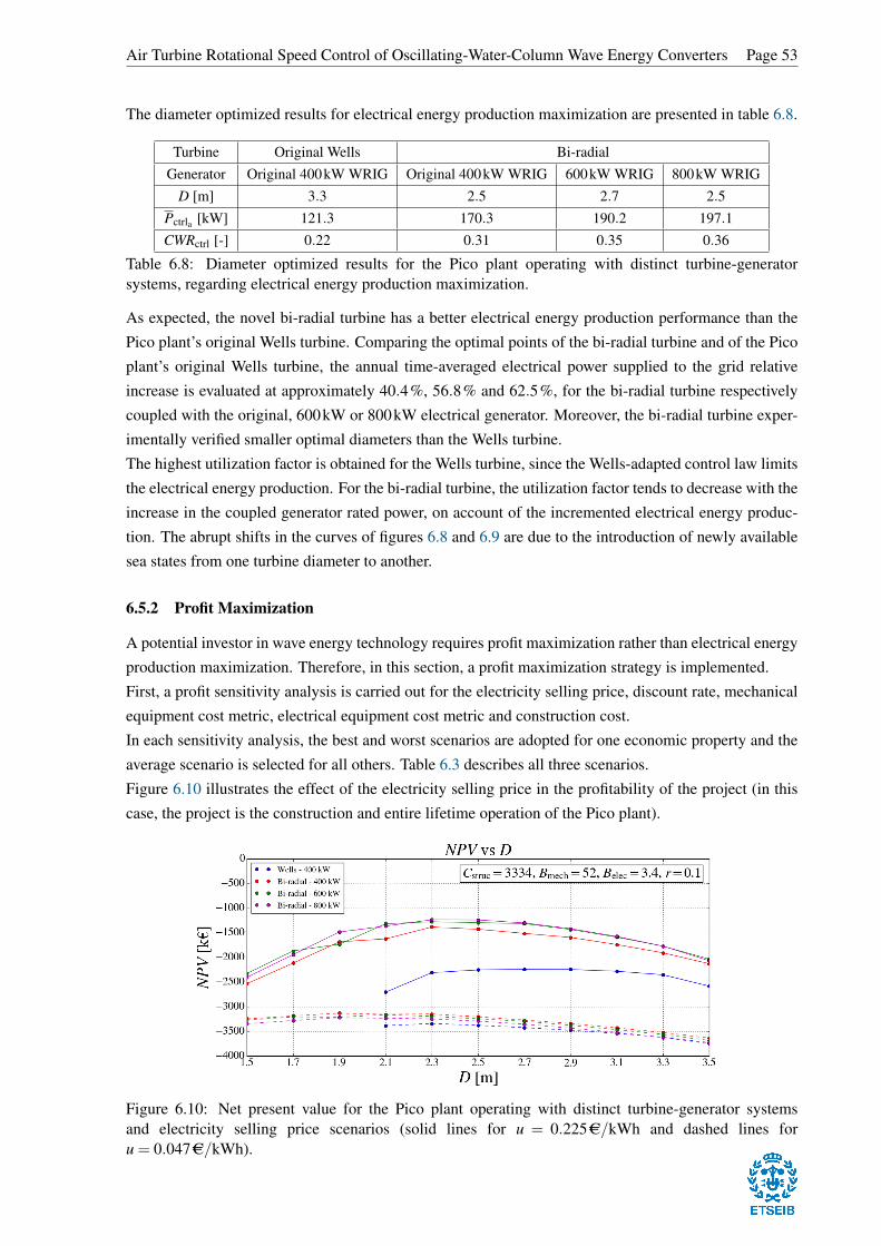
Air Turbine Rotational Speed Control of Oscillating-Water-Column Wave Energy Converters Page 53
The diameter optimized results for electrical energy production maximization are presented in table 6.8.
Turbine Original Wells Bi-radialGenerator Original 400kW WRIG Original 400kW WRIG 600kW WRIG 800kW WRIG
D [m] 3.3 2.5 2.7 2.5Pctrla [kW] 121.3 170.3 190.2 197.1CWRctrl [-] 0.22 0.31 0.35 0.36
Table 6.8: Diameter optimized results for the Pico plant operating with distinct turbine-generatorsystems, regarding electrical energy production maximization.
As expected, the novel bi-radial turbine has a better electrical energy production performance than the
Pico plant’s original Wells turbine. Comparing the optimal points of the bi-radial turbine and of the Pico
plant’s original Wells turbine, the annual time-averaged electrical power supplied to the grid relative
increase is evaluated at approximately 40.4%, 56.8% and 62.5%, for the bi-radial turbine respectively
coupled with the original, 600kW or 800kW electrical generator. Moreover, the bi-radial turbine exper-
imentally verified smaller optimal diameters than the Wells turbine.
The highest utilization factor is obtained for the Wells turbine, since the Wells-adapted control law limits
the electrical energy production. For the bi-radial turbine, the utilization factor tends to decrease with the
increase in the coupled generator rated power, on account of the incremented electrical energy produc-
tion. The abrupt shifts in the curves of figures 6.8 and 6.9 are due to the introduction of newly available
sea states from one turbine diameter to another.
6.5.2 Profit Maximization
A potential investor in wave energy technology requires profit maximization rather than electrical energy
production maximization. Therefore, in this section, a profit maximization strategy is implemented.
First, a profit sensitivity analysis is carried out for the electricity selling price, discount rate, mechanical
equipment cost metric, electrical equipment cost metric and construction cost.
In each sensitivity analysis, the best and worst scenarios are adopted for one economic property and the
average scenario is selected for all others. Table 6.3 describes all three scenarios.
Figure 6.10 illustrates the effect of the electricity selling price in the profitability of the project (in this
case, the project is the construction and entire lifetime operation of the Pico plant).
Figure 6.10: Net present value for the Pico plant operating with distinct turbine-generator systemsand electricity selling price scenarios (solid lines for u = 0.225AC/kWh and dashed lines foru = 0.047AC/kWh).

Page 54 Dissertation
Break-even, i.e., null net present value, is not achieved for any of the tested electricity selling price
scenarios. This is the same as to say that, in an average scenario and for electricity selling prices ranging
from u = 0.047AC/kWh to u = 0.225AC/kWh, the project is economically unprofitable.
Table 6.9 presents the break-even electricity selling prices uBe and respective diameters.
Turbine Original Wells Bi-radialGenerator Original 400kW WRIG Original 400kW WRIG 600kW WRIG 800kW WRIG
D [m] 3.1 2.3 2.7 2.5uBe [AC/kWh] 0.548 0.365 0.344 0.333
Table 6.9: Break-even electricity selling price for the Pico plant operating with distinct turbine-generatorsystems.
The effect of the discount rate on the project’s profitability is illustrated in figure 6.11.
Figure 6.11: Net present value for the Pico plant operating with distinct turbine-generator systems anddiscount rate scenarios (solid lines for r = 5% and dashed lines for r = 15%).
Again, the break-even point is not verified for any of the tested scenarios. It is important to verify if any
of the tested scenarios demonstrates a positive return on investment in the absence of additional profits,
i.e., exhibits a positive internal rate of return.
The break-even discount rate is identical to the internal rate of return. In table 6.10, the internal rates of
return and respective diameters are presented.
Turbine Original Wells Bi-radialGenerator Original 400kW WRIG Original 400kW WRIG 600kW WRIG 800kW WRIG
D [m] 2.9 2.3 2.3 2.5IRR [%] −4.8 −0.9 −0.4 −0.1
Table 6.10: Internal rate of return for the Pico plant operating with distinct turbine-generator systems.
Reducing the discount rate, the operational cash flows are sharply increased. In spite of that, out of all
the turbine-generator systems tested in table 6.10, none demonstrated a positive internal rate of return.
For the bi-radial turbine coupled with the 800kW electrical generator, an almost positive internal rate
of return of IRR = −0.1% was obtained. This means the project, without additional profits, is able to
generate a nearly positive return on investment, which is very promising.
Determining how the project’s profitability is altered by the cost of the mechanical equipment is specially
important, since it is for these components that a great part of the current academic research is performed.

Air Turbine Rotational Speed Control of Oscillating-Water-Column Wave Energy Converters Page 55
Figure 6.12 represents the effect of the mechanical equipment cost metric on the project’s profitability.
Figure 6.12: Net present value for the Pico plant operating with distinct turbine-generator systems andmechanical equipment cost metric scenarios (solid lines for Bmech = 25kAC/m2 and dashed lines forBmech = 78kAC/m2).
Independently of the tested turbine-generator system, break-even is not attained. Therefore, in the aver-
age scenario, it is impossible to transform the project into an economically profitable venture by solely
altering the cost of the turbine and valve systems.
The severe impact of the mechanical equipment cost metric on the turbine diameter optimization is
particularly visible when comparing the best and worst scenario curves in figure 6.12. Increasing the
mechanical cost metric, the optimal diameter tends to decrease, since the added generated revenue for
larger turbine diameters no longer compensates for their parallel cost increase.
In figure 6.13, the effect of the electrical equipment cost metric on the project’s profitability is illustrated.
Figure 6.13: Net present value for the Pico plant operating with distinct turbine-generator systemsand electrical equipment cost metric scenarios (solid lines for Belec = 2.5kAC/m0.7 and dashed lines forBelec = 4.2kAC/m0.7).
Again, there is no electrical equipment cost metric so that the project is economically profitable.
It is possible to observe that increasing the electrical equipment cost metric favors the utilization of
the 600kW electrical generator in preference to the 800kW electrical generator. This is so because,
eventually, the additional electrical energy production resultant from the increase of the generator rated
power no longer compensates for the increment in the cost of the electrical equipment.

Page 56 Dissertation
Figure 6.14 illustrates the effect of the construction cost on the project’s profitability.
Figure 6.14: Net present value for the Pico plant operating with distinct turbine-generator systems andconstruction cost scenarios (solid lines for Cstruc = 1667kAC and dashed lines for Cstruc = 5001kAC).
Analyzing the disparity between the best and worst scenario curves in figure 6.14, the construction cost’s
importance to the profitability of the project is made clear. However, note that for the best scenario,
considering a 50% construction cost reduction, break-even is not achieved.
Although the consideration of even lower construction costs is optimistic, it is important to determine
the construction cost estimates that result in a positive profitability for the project. Accordingly, the
break-even construction costs CstrucBe and respective diameters are shown in table 6.11.
Turbine Original Wells Bi-radialGenerator Original 400kW WRIG Original 400kW WRIG 600kW WRIG 800kW WRIG
D [m] 2.5 2.3 2.3 2.3CstrucBe [kAC] 244 846 880 874
Table 6.11: Break-even construction cost for the Pico plant operating with distinct turbine-generatorsystems.
Examining the results from figure 6.12 and those from figure 6.14 and table 6.11, it is possible to compare
the effect of the mechanical equipment cost metric and the construction cost on the project’s profitability.
Overall, these results reinforce the idea that the wave energy technology readiness level is more depen-
dent on the reduction of the construction cost than on the reduction of the mechanical equipment cost.
The construction of an OWC WEC presently represents the majority of its capital costs. As a result,
some authors propose the construction cost be diluted by incorporating the OWC WEC into a breakwa-
ter, which furthermore reduces the O&M costs [4]. The results in figure 6.14 confirm the importance of
the breakwater-OWC solution, as well as any similar solutions that aim to mitigate the construction cost,
since this property has a significant economic impact on profitability.
So far, the performed experiments focused on the effect of the project’s most important economic prop-
erties on its profitability. These results are relevant, but only describe the action of one property at a
time. For a complete profit maximization analysis, potential economic frameworks should additionally
be studied: this is accomplished through the examination of the three scenarios presented in table 6.3.
Take into account that the worst and best scenarios may be overly pessimistic and optimistic, respec-
tively. For that reason, the average scenario is also considered.

Air Turbine Rotational Speed Control of Oscillating-Water-Column Wave Energy Converters Page 57
The results for the project’s profitability in the best scenario are illustrated in figure 6.15.
Figure 6.15: Net present value for the Pico plant operating with distinct turbine-generator systems in thebest scenario.
The project can be economically profitable for all turbine-generator systems in the best scenario.
Table 6.12 presents, for the best scenario, the optimal diameters and corresponding net present value,
internal rate of return and payback period profit metrics.
Turbine Original Wells Bi-radialGenerator Original 400kW WRIG Original 400kW WRIG 600kW WRIG 800kW WRIG
D [m] 3.1 2.3 2.7 2.5NPV [kAC] 425 1596 1895 2010IRR [%] 7.1 12.5 13.3 13.6
PBP [year] 16.7 10.4 9.8 9.6
Table 6.12: Net present value, internal rate of return and payback period for the Pico plant operating withdistinct turbine-generator systems in the best scenario.
In the best scenario, the bi-radial turbine demonstrates a better economic performance than the Wells
turbine, independently of the coupled electrical generator. This is because, in this scenario, the sharply
reduced mechanical and electrical equipment costs, combined with the high electricity selling prices,
favor the operation of a turbine with a higher electrical energy production. In this regard, the bi-radial
turbine is superior to the Wells turbine. This is proven by the electrical energy production maximization
results, regarding all tested turbine-generator systems, in figure 6.8.
The best scenario results, in figure 6.15 and table 6.12, combined with the sensitivity analysis results
for the electricity selling price and the construction cost, respectively presented in figures 6.10 and 6.14,
demonstrate that a high electricity selling price and low construction cost are fundamental for the eco-
nomic profitability of the project. However, these conditions are only possible if beneficial governmental
policies exist to ensure the competitiveness of wave energy technology in the energy generation market.
In spite of its relevance, the best scenario is fairly optimistic. Apart from low amounts for the electrical
and mechanical equipment costs, construction cost and discount rate, it also assumes a governmental
subsidy for the electricity selling price, equal to the amount originally designated for the Pico plant.
Concerning the remaining tests, less optimistic frameworks need to be analyzed.

Page 58 Dissertation
The profitability of the project in the worst scenario is illustrated in figure 6.16.
Figure 6.16: Net present value for the Pico plant operating with distinct turbine-generator systems in theworst scenario.
The worst scenario optimal diameters and respective profit metrics are presented in table 6.13.
Turbine Original Wells Bi-radialGenerator Original 400kW WRIG Original 400kW WRIG 600kW WRIG 800kW WRIG
D [m] 2.1 1.9 1.7 1.9NPV [kAC] −4901 −4699 −4756 −4829IRR [%] −26.5 −14.1 −15.1 −13.6
Table 6.13: Net present value and internal rate of return for the Pico plant operating with distinctturbine-generator systems in the worst scenario.
The results in figure 6.16 and table 6.13 demonstrate that, if reasonable economic conditions are not met,
the construction and operation of an OWC WEC can result in a disastrous economic venture. Hence,
before the project’s launch, it is paramount to ensure that its economic environment is sound.
In figure 6.17 is the project’s profitability in the average scenario (the most realistic economic conditions).
Figure 6.17: Net present value for the Pico plant operating with distinct turbine-generator systems in theaverage scenario.
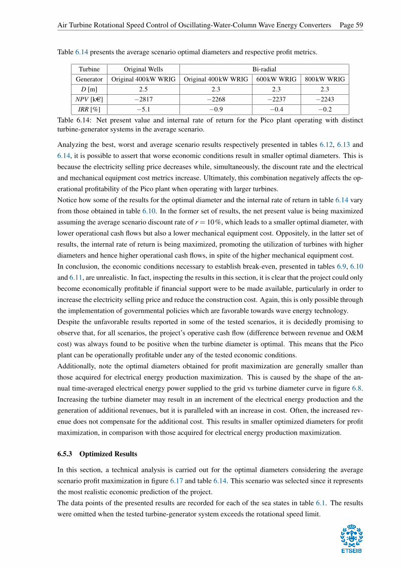
Air Turbine Rotational Speed Control of Oscillating-Water-Column Wave Energy Converters Page 59
Table 6.14 presents the average scenario optimal diameters and respective profit metrics.
Turbine Original Wells Bi-radialGenerator Original 400kW WRIG Original 400kW WRIG 600kW WRIG 800kW WRIG
D [m] 2.5 2.3 2.3 2.3NPV [kAC] −2817 −2268 −2237 −2243IRR [%] −5.1 −0.9 −0.4 −0.2
Table 6.14: Net present value and internal rate of return for the Pico plant operating with distinctturbine-generator systems in the average scenario.
Analyzing the best, worst and average scenario results respectively presented in tables 6.12, 6.13 and
6.14, it is possible to assert that worse economic conditions result in smaller optimal diameters. This is
because the electricity selling price decreases while, simultaneously, the discount rate and the electrical
and mechanical equipment cost metrics increase. Ultimately, this combination negatively affects the op-
erational profitability of the Pico plant when operating with larger turbines.
Notice how some of the results for the optimal diameter and the internal rate of return in table 6.14 vary
from those obtained in table 6.10. In the former set of results, the net present value is being maximized
assuming the average scenario discount rate of r = 10%, which leads to a smaller optimal diameter, with
lower operational cash flows but also a lower mechanical equipment cost. Oppositely, in the latter set of
results, the internal rate of return is being maximized, promoting the utilization of turbines with higher
diameters and hence higher operational cash flows, in spite of the higher mechanical equipment cost.
In conclusion, the economic conditions necessary to establish break-even, presented in tables 6.9, 6.10
and 6.11, are unrealistic. In fact, inspecting the results in this section, it is clear that the project could only
become economically profitable if financial support were to be made available, particularly in order to
increase the electricity selling price and reduce the construction cost. Again, this is only possible through
the implementation of governmental policies which are favorable towards wave energy technology.
Despite the unfavorable results reported in some of the tested scenarios, it is decidedly promising to
observe that, for all scenarios, the project’s operative cash flow (difference between revenue and O&M
cost) was always found to be positive when the turbine diameter is optimal. This means that the Pico
plant can be operationally profitable under any of the tested economic conditions.
Additionally, note the optimal diameters obtained for profit maximization are generally smaller than
those acquired for electrical energy production maximization. This is caused by the shape of the an-
nual time-averaged electrical energy power supplied to the grid vs turbine diameter curve in figure 6.8.
Increasing the turbine diameter may result in an increment of the electrical energy production and the
generation of additional revenues, but it is paralleled with an increase in cost. Often, the increased rev-
enue does not compensate for the additional cost. This results in smaller optimized diameters for profit
maximization, in comparison with those acquired for electrical energy production maximization.
6.5.3 Optimized Results
In this section, a technical analysis is carried out for the optimal diameters considering the average
scenario profit maximization in figure 6.17 and table 6.14. This scenario was selected since it represents
the most realistic economic prediction of the project.
The data points of the presented results are recorded for each of the sea states in table 6.1. The results
were omitted when the tested turbine-generator system exceeds the rotational speed limit.

Page 60 Dissertation
Figure 6.18 illustrates the time-averaged turbine efficiency for all tested turbine-generator systems.
Figure 6.18: Time-averaged turbine efficiency for the Pico plant operating with the diameter optimizedturbine-generator systems.
For more energetic sea states, the average turbine efficiency decreases. This is because the imposed con-
straints in the turbine rotational speed prevent the optimal rotational speed from being reached. Regard-
ing the Pico plant’s original Wells turbine, the rotational speed is constrained through the Wells-adapted
control law in equation (5.6). For the bi-radial turbine, the rotational speed constraint is a result of the
generator rated power being too low, which affects the cube control law in equation (5.4).
If the aforementioned constraints are not imposed, the rotational speed of the turbine will tend to an un-
constrained amount. For the constrained and unconstrained turbine-generator systems, the time-averaged
turbine rotational speed is shown in figure 6.19.
Figure 6.19: Time-averaged turbine rotational speed for the Pico plant operating with the diameteroptimized constrained and unconstrained turbine-generator systems.
As expected, for the unconstrained case, the rotational speed of the Pico plant’s original Wells turbine is
considerably larger than that of the bi-radial turbine [10]. This helps to validate the implementation of
the Wells-adapted control law: without it, the rotational speed of the Wells turbine increases extremely
fast and rapidly crosses the limit defined in equation (5.5).

Air Turbine Rotational Speed Control of Oscillating-Water-Column Wave Energy Converters Page 61
On the other hand, the rotational speed of the bi-radial turbine tends to be lower for the unconstrained
case. The rotational speed control of the bi-radial turbine is evidently hindered by its sizable moment of
inertia of the rotating parts and the low generator rated power.
The electrical energy production is somewhat affected for all tested turbine-generator systems. Note
that, if no constraints existed, the Pico plant would be able to operate under the most energetic sea state
(according to table 6.1, it is responsible for approximately 4% of the annual wave power).

Page 62 Dissertation

Air Turbine Rotational Speed Control of Oscillating-Water-Column Wave Energy Converters Page 63
7 Preliminary Planning and Costs — Pico Plant Case Study
A brief planning structure and cost analysis of the Pico plant case study are presented in this section.
Specifically, the present day development of a fixed structure OWC WEC, identical to the Pico plant, is
studied. The planning is described from the initial conceptualization and design stage to the completion
of the construction stage. The cost analysis additionally includes the operation of the plant.
First, in section 7.1, the planning of the project is detailed.
Second, section 7.2 describes the project’s costs. In the present work, several economic conditions were
studied, in the form of the scenarios characterized through table 6.3. In the cost analysis performed here,
the most realistic economic conditions are considered, which corresponds to the average scenario.
7.1 Project Planning
The planning for the present day development of a plant identical to the Pico plant is illustrated in the
form of a Gantt chart in figure 7.1. The data regarding the duration of each stage is based on [6].
Figure 7.1: Gantt chart from the start of conceptualization to the end of civil construction for thedevelopment of the present day Pico plant.
In the development of a present day Pico plant, the first stage of the project regards the conceptualization
of the plant, which is divided into four sub-stages.
Firstly, the location where the plant will be erected is selected. It should be a location that guarantees the
best balance between the magnitude and seasonality of the wave energy resource.
Secondly, basic studies concerning the feasibility of the project at the selected location are carried out.
Additionally, the design specifications of the plant are defined, considering its hydrodynamic modelling,
structural design, mechanical equipment and electrical equipment.
Lastly, all permits and approvals for the construction of the plant are obtained. This is one of the most
prolonged periods in the conceptualization stage.
The civil construction of the present day Pico plant is implemented in two sub-stages: the bidding process
and the construction itself.
The bidding process is normally public and aims to elect, out of the candidate project developers, the one
whose project provides the best balance between cost and quality.
7.2 Cost Analysis
The costs related to the development of a present day Pico plant are now analyzed. As aforementioned
in section 7, the average scenario economic conditions are studied.

Page 64 Dissertation
The costs of the project can either be capital or operational costs. For the cost analysis performed in this
section, the Pico plant is assumed to operate with the bi-radial turbine of diameter D = 2.5m coupled
with the 800kW electrical generator, which resulted in the highest internal rate of return in the average
scenario, according to the sensitivity analysis in table 6.10.
The capital costs of the project mainly result from the construction of the plant and procurement of the
mechanical and electrical equipment, being generally described in table 6.3 and formulated in section
5.2.2. The capital costs of the control and instrumentation equipment and those regarding the conceptu-
alization stage are disregarded since they are negligible in comparison with the aforementioned capital
costs and considering their information is lacking due to their common use in non-disclosed projects.
In table 7.1, the capital costs of the project are described.
Project component Capital cost [kAC]
Construction 3334
Mechanical equipment 325
Electrical equipment 366
Total 4025
Table 7.1: Capital costs of the Pico plant operating with the bi-radial turbine and the 800kW electricalgenerator in the average scenario.
As was remarked in section 6.5.2, the construction cost represents the majority of the capital costs in the
implementation of an OWC WEC. Analyzing table 7.1 it is possible to observe that, for this section’s
studied case, the construction cost stands for approximately 82.8% of the total capital cost.
The project’s operational costs, presented in table 7.2, are expressed rewriting equation (5.17) for the
studied case and considering the adjustment for inflation at the predicted inflation rate of ri = 1.1%
(approximate average Portuguese inflation rate for the last decade).
Year Operational cost [kAC] Year Operational cost [kAC]1 21.4 11 23.92 21.7 12 24.23 21.9 13 24.44 22.1 14 24.75 22.4 15 25.06 22.6 16 25.27 22.9 17 25.58 23.1 18 25.89 23.4 19 26.110 23.6 20 26.4
Table 7.2: Annual operational cost of the Pico plant operating with the bi-radial turbine and the 800kWelectrical generator in the average scenario.
Observing the results for the capital and operational costs, respectively presented in tables 7.1 and 7.2, it
is possible to assert that, in the studied case, the capital cost represents approximately 89.4% of the total
project’s cost, while the operational cost accounts for the remaining 10.6%.
Both the capital and operational costs obtained in this section can be assumed to generally estimate
the costs incorporated in analogous projects, specifically those regarding the implementation of fixed
structure OWC WECs.

Air Turbine Rotational Speed Control of Oscillating-Water-Column Wave Energy Converters Page 65

Page 66 Dissertation
8 Environmental Impact — Pico Plant Case Study
Whenever studying a renewable energy generation source, it is essential to examine its environmental
impact. In this section, a concise environmental analysis of wave energy technology is carried out,
particularly in what regards the present day implementation of a fixed structure OWC WEC, identical to
the Pico plant. As in section 7, the case study of the Pico plant operating with the bi-radial turbine of
diameter D = 2.5m and the 800kW electrical generator is considered in the calculations presented.
The environmental impact analysis of the project is divided into two sections: determination of avoided
greenhouse gas and atmospheric pollutant emissions; examination of the socioeconomic impact.
8.1 Avoided Emissions
While the operation of a WEC emits no greenhouse gases or any atmospheric pollutants whatsoever,
other stages of its life cycle are responsible for these emissions. To adequately compare the environmen-
tal impact of wave energy technology with that of other energy generation technologies, the emissions
resultant from the entire life cycle of every analyzed case must be considered.
In this section, the amount of avoided emissions in regard to the Portuguese electricity supply mix is
defined. Its emission factors are 172g CO2-eq/kWh, 0.18g SO2-eq/kWh and 0.6g NOx-eq/kWh, approx-
imately, according to [37] and [38].
Due to scarce existent information regarding the emissions of wave energy technology, the work in [39],
specifically developed for the Ocean Swell Powered Renewable Energy fixed structure OWC WEC, is
treated as generally characteristic of wave energy technology. Then, the emission factors of wave energy
technology are, approximately, 14g CO2-eq/kWh, 0.10g SO2-eq/kWh and 0.05g NOx-eq/kWh.
Operating the present day Pico plant with the aforementioned turbine-generator system, the annual elec-
trical power supplied to the grid Pctrla = 197.1kW during the entirety of the expected lifetime of the
plant, estimated at n = 20years, results in a total electrical energy generation of 34.53GWh. In com-
parison with the Portuguese electricity supply mix, this results in the avoidance of greenhouse gas and
atmospheric pollutant emissions of approximately 5.46kt CO2-eq, 2.76t SO2-eq and 18.99t NOx-eq.
8.2 Socioeconomic Impact
The avoided emissions by the present day Pico plant, studied in section 8.1, are representative of a
beneficial social effect of wave energy technology. However, the present day Pico plant incorporates
other outcomes that produce a socioeconomic impact.
First, some of the most common negative consequences generally pointed out in wave energy technology
are addressed. Examples of these negative effects are: sediment disturbance, modification of the existent
ecosystem and acoustic noise. The aforementioned negative impacts are either not verified in harmful
magnitudes or there is insufficient information to assess them [39].
Apart from the aforementioned reduction in greenhouse gas and atmospheric pollutant emissions, some
examples of the beneficial social and economic effects resultant from the implementation of the present
day Pico plant are: firstly, growth of the local economy due to the local population’s employment in
the plant’s construction and operation; secondly, nationwide operationally cheaper energy generation;
thirdly, creation of a unique wave energy technology R&D hub, which can globally attract academic
researchers and tourism and ultimately lead to the further development of the local region and its people.

Air Turbine Rotational Speed Control of Oscillating-Water-Column Wave Energy Converters Page 67

Page 68 Dissertation
9 Conclusions
The present work’s main objective was to develop the numerical model of the Pico wave power plant.
Then, three other primary outcomes were established: firstly, the validation of a method able to model
the radiation flow rate; secondly, the implementation and comparison of rotational speed control applied
to an OWC WEC operating with the Wells and bi-radial turbines; thirdly, the optimization of the turbine
diameter derived from the rotational speed control results, for distinct optimization strategies and poten-
tial economic frameworks of wave energy technology.
In the Pico wave power plant case study, the application of Prony’s method in modelling the radiation
flow rate produced the best results. Both the relative root-mean-square error and the correlation coeffi-
cient of the pneumatic power available to the turbine were experimentally verified to fall into acceptable
intervals. In fact, the application of Prony’s method with fifteen complex negative exponential func-
tions demonstrated a relative root-mean-square error of RRMSEpneu ≤ 1% and a correlation coefficient
of Rpneu ≥ 0.97 for the wave frequencies responsible for 99.7% of the total energy in the case study’s
location. Moreover, it verified a 94.1% average computational time reduction relatively to the analytical
computation of the radiation flow rate. The satisfactory results obtained for the error and computational
time conclusively validate the studied application of Prony’s method.
The case study implementation of rotational speed control evidenced the superiority of the bi-radial tur-
bine’s energy extraction performance in comparison to the Wells turbine. Coupling both turbines with
the case study’s original electrical generator, of rated power Pratedgen = 400kW, the annual time-averaged
electrical power supplied to the grid utilizing the bi-radial turbine registered a relative growth of 40.4%
when compared to the utilization of the Wells turbine. It was additionally verified that the optimal diam-
eters of the bi-radial turbine design were considerably smaller than those of the Wells turbine design.
Moreover, it was experimentally verified that, in the real environment conditions of the case study, the
rated power of the electrical generator was limiting the electrical energy production when the bi-radial
turbine was in operation. Hence, the additional utilization of a 600kW and an 800kW generator were
studied. These resulted, respectively, in a 56.8% and 62.5% relative increase in the annual time-averaged
electrical power supplied to the grid, when compared to the original Wells turbine-generator system.
Lastly, the turbine diameter was optimized for profit maximization under the best, worst and average
potential economic scenarios for wave energy technology. A straightforward analysis of the results leads
to the conclusion that wave energy technology is still at a low technology readiness level: for example, in
an average scenario, unfavorable results were obtained for the best net present value NPV = −2237kAC
or for the highest break-even construction cost CstrucBe = 880kAC. Nevertheless, the best internal rate
of return obtained in average economic conditions is IRR = −0.1% and, although negative, means the
project can nearly generate positive returns on investment. Moreover, the case study plant was found to
be operationally profitable for any of the tested economic frameworks if the optimal turbine diameter is
selected. These results are specially encouraging and testify to the potential of wave energy technology.
Apart from their value in the analysis of the selected case study, the overall results from the turbine
diameter optimization for profit maximization generally describe the present economic framework for
wave energy technology implementation, particularly for one of the most developed WEC designs: the
fixed structure OWC. Thus, it can be stated that the fundamental identified key barriers to the current im-
plementation of wave energy technology were its low electricity selling price and high construction cost.
A clear economic solution for both barriers is to promote financial support in wave energy technology,

Air Turbine Rotational Speed Control of Oscillating-Water-Column Wave Energy Converters Page 69
which is strongly dependent on governmental policies. Example of financial support measures are wave
energy generated electricity tax benefits, wave energy converter construction partial funding and invest-
ment in cost reduction wave energy technology R&D. Regarding the construction cost barrier, this cost
can be diluted if the WEC is incorporated into a breakwater, in case it is comprised of a fixed structure.
This solution, already proposed by several authors, is able to reduce construction and O&M costs and its
implementation is essential if wave energy technology is to mature and become economically profitable.
In conclusion, the results obtained in this work are demonstrative that, despite promising, wave energy
technology is still at an early stage of its development and requires financial support to overcome its
current technical and economic barriers. Whether this technology matures or becomes irrelevant in the
foreseeable future will ultimately depend on governmental policies.
Finally, along with the dissertation, future lines of research are suggested:
• Improve upon the Prony’s method radiation flow rate model presented in this work by, for exam-
ple, considering a greater number of complex negative exponential functions and increasing the
modelled time for the memory effect.
• Test the influence of the computational time step reduction on error convergence, for the classic
Runge-Kutta numerical implementation of the OWC WEC’s uniform pressure model dynamics.
• Extend the rotational speed control model to take into account the effect of the grid supplied load
in the electrical generator’s efficiency.
• Develop comparative analyses, analogous to the present work, for other self-rectifying turbine
designs (for example, contra-rotating Wells, biplane Wells, variable pitch Wells and Deniss-Auld).
• Research further into other forms of control for a WEC operating with an air turbine, as for exam-
ple reactive phase control and phase control by latching.
• Study the economic impact of the incorporation of fixed structure WECs in a breakwater.

Page 70 Dissertation

Air Turbine Rotational Speed Control of Oscillating-Water-Column Wave Energy Converters Page 71
10 Appreciations
Neither the beginning, development or conclusion of this work would have been possible without the
support of professors João Carlos de Campos Henriques and Duarte Pedro Mata de Oliveira Valério.
Their continual and unfaltering assistance has truly been key in every single progress made throughout
the entirety of this dissertation and for that I would like to offer them my sincerest gratitude.
This work is first and foremost dedicated to Pedro Paulo Valente Gentil Soares Branco, Graça Maria
Duarte Serejo, Mariana Serejo Soares Branco and Inês Ferreira Casaleiro Nogueira de Brito, whose un-
conditional assistance I deeply value and could not have succeeded without.
A special thanks is also in order to my friends Afonso Botelho, António Coelho, António Pinto, Daniel
Lopes, David Ferreira, Duarte Delgado, Manuel Domingues and Ricardo Bento, for their endless cama-
raderie and availability.
An additional thanks to Carlos Costa and Leonel Verdasca for their help in the work developed and to all
my InnoEnergy Renewable Energy colleagues for their energizing open mindedness.
Finally, I would also like to acknowledge professor António Franco de Oliveira Falcão, who not only
introduced me to wave energy technology, but is someone who I profoundly appreciate and respect.

Page 72 Dissertation

Air Turbine Rotational Speed Control of Oscillating-Water-Column Wave Energy Converters Page 73
Bibliography
[1] Gunn K. and Stock-Williams C. Quantifying the global wave power resource. Renewable Energy,
44:296–304, 2012.
[2] Guedes Soares C., Rute Bento A., Gonçalves M., Silva D., and Martinho P. Numerical evaluation of
the wave energy resource along the Atlantic European coast. Computers & Geosciences, 71:37–49,
2014.
[3] Pérez-Collazo C., Greaves D., and Iglesias G. A review of combined wave and offshore wind
energy. Renewable and Sustainable Energy Reviews, 42:141–153, 2015.
[4] Falcão A. F. de O. Wave energy utilization: a review of the technologies. Renewable and Sustain-
able Energy Reviews, 14(3):899–918, 2010.
[5] Pecher A. and Kofoed J. P. Handbook of ocean wave energy. Springer London, 2017.
[6] Falcão A. F. de O., Sarmento A. J. N. A., Gato L. M. C., and Brito-Melo A. The Pico OWC
wave power plant: its lifetime from conception to closure 1986–2018. Applied Ocean Research,
98:102–104, 2020.
[7] Falcão A. F. de O. The shoreline OWC wave power plant at the Azores. In Proceedings of 4th
European Wave Energy Conference, pages 42–47, 2000.
[8] Non Nuclear Energy Programme JOULE III. European wave energy pilot plant on the island of
Pico, Azores, Portugal. Phase two: equipment. Publishable Report. Contract no: JOR3-CT95-0012,
1998.
[9] Falcão A. F. de O. and Henriques J. C. C. Oscillating-water-column wave energy converters and air
turbines: a review. Renewable Energy, 85:1391–1424, 2016.
[10] Falcão A. F. de O., Henriques J. C. C., and Gato L. M. C. Air turbine optimization for a bottom-
standing oscillating-water-column wave energy converter. Journal of Ocean Engineering and Ma-
rine Energy, 2(4):459–472, 2016.
[11] Justino P. A. P. and Falcão A. F. de O. Rotational speed control of an OWC wave power plant.
Journal of Offshore Mechanics and Arctic Engineering, 121:65–70, 1999.
[12] Falcão A. F. de O. Modelling of wave energy conversion lecture notes. Unpublished Publication,
2019.
[13] Falcão A. F. de O. and Gato L. M. C. Air turbines. Comprehensive Renewable Energy, 8:111–149,
2012.
[14] Falcão A. F. de O. Control of an oscillating-water-column wave power plant for maximum energy
production. Applied Ocean Research, 24(2):73–82, 2002.

Page 74 Dissertation
[15] Falnes J. Ocean waves and oscillating systems: linear interactions including wave-energy extrac-
tion. Cambridge University Press, 2002.
[16] Falcão A. F. de O. Modelling of wave energy conversion. Unpublished Presentation, 2019.
[17] White F. M. Fluid mechanics. Mc Graw-Hill, 2011.
[18] André J. M. C. S. Apontamentos de ondas de superfície livre. AEIST Press, 2019.
[19] Holthuijsen L. H. Waves in oceanic and coastal waters. Cambridge University Press, 2010.
[20] Goda Y. Random seas and design of maritime structures. World Scientific, 2010.
[21] Pain H. J. The physics of vibrations and waves. Acoustical Society of America, 2005.
[22] Park K. I. Fundamentals of probability and stochastic processes with applications to communica-
tions. Springer, 2018.
[23] Falcão A. F. de O. and Rodrigues R. J. A. Stochastic modelling of OWC wave power plant perfor-
mance. Applied Ocean Research, 24(2):59–71, 2002.
[24] Henriques J. C. C., Portillo J. C. C., Sheng W., Gato L. M. C., and Falcão A. F. de O. Dynamics
and control of air turbines in oscillating-water-column wave energy converters: analyses and case
study. Renewable and Sustainable Energy Reviews, 112:571–589, 2019.
[25] Sarmento A. J. N. A. and Falcão A. F. de O. Wave generation by an oscillating surface-pressure
and its application in wave-energy extraction. Journal of Fluid Mechanics, 150:467–485, 1985.
[26] Dixon S. L. Fluid mechanics, thermodynamics of turbomachinery. Butterworth-Heinemann, 1998.
[27] Atkinson K. E. An introduction to numerical analysis. John Wiley & Sons, 2008.
[28] Rodríguez A., Rodrigo L., Guillén E., Ascariz J. M., Jiménez J. M., and Boquete L. Coding Prony’s
method in MATLAB and applying it to biomedical signal filtering. BMC Bioinformatics, 19(1):1–
14, 2018.
[29] Sheng W., Alcorn R., and Lewis A. A new method for radiation forces for floating platforms in
waves. Ocean Engineering, 105:43–53, 2015.
[30] Falcão A. F. de O. Stochastic modelling in wave power-equipment optimization: maximum energy
production versus maximum profit. Ocean Engineering, 31(11-12):1407–1421, 2004.
[31] Brito-Melo A., Hofmann T., Sarmento A. J. N. A., Clément A. H., and Delhommeau G. Numerical
modelling of OWC-shoreline devices including the effect of surrounding coastline and non-flat
bottom. International Journal of Offshore and Polar Engineering, 11(02), 2001.
[32] Falcão A. F. de O. and Justino P. A. P. OWC wave energy devices with air flow control. Ocean
Engineering, 26(12):1275–1295, 1999.

Air Turbine Rotational Speed Control of Oscillating-Water-Column Wave Energy Converters Page 75
[33] Gato L. M. C., Henriques J. C. C., Carrelhas A. A. D., Lopes B. S., Varandas J., and Fay F. X.
Turbine and electrical equipment performance and reliability in shoreline OWC wave plant. Deliv-
erable D3.3 of the HORIZON 2020 project OPERA. EC Grant agreement no: 654444, IST: Lisbon,
Portugal, 2018.
[34] Conselho de Reguladores do MIBEL. Estudo sobre comparação dos preços MIBEL (à vista e a
prazo) com outros mercados europeus e a sua relação com o mercado único. Published Report,
2019.
[35] Torre-Enciso Y., Ortubia I., Aguilleta L. I., and Marqués J. Mutriku wave power plant: from the
thinking out to the reality. In Proceedings of the 8th European Wave and Tidal Energy Conference,
Uppsala, Sweden, volume 710, pages 319–329, 2009.
[36] Despotovic M., Nedic V., Despotovic D., and Cvetanovic S. Evaluation of empirical models for
predicting monthly mean horizontal diffuse solar radiation. Renewable and Sustainable Energy
Reviews, 56:246–260, 2016.
[37] International Energy Agency. CO2 intensity of energy mix (CO2/TES), Portugal 1990-
2019. Available online at: https://www.iea.org/data-and-statistics?country=
PORTUGAL&fuel=CO2%20emissions&indicator=CO2Intensity, 2020 (accessed Oc-
tober 15, 2020).
[38] Organisation for Economic Co-operation and Development. Emissions of air pollutants,
Portugal 1990-2018. Available online at: https://stats.oecd.org/Index.aspx?
DataSetCode=AIR_EMISSIONS, 2020 (accessed October 15, 2020).
[39] Thorpe T. W. A brief review of wave energy. Harwell Laboratory, Energy Technology Support Unit
London, 1999.
[40] Bando Y. How to move Canon EF lenses. Unpublished Presentation, 2019.
[41] Moran M. J., Shapiro H. N., Boettner D. D., and Bailey M. B. Fundamentals of engineering
thermodynamics. John Wiley & Sons, 2010.
[42] Gato L. M. C., Henriques J. C. C., Carrelhas A. A. D., Lopes B. S., Fay F. X., Pujana A., Ruiz-
Minguela P., Kelly J., Mueller M., and Aldaiturriaga E. Shoreline OWC wave power plant control
algorithms. Deliverable D4.2 of the HORIZON 2020 project OPERA. EC Grant agreement no:
654444, TECNALIA: Derio, Spain, 2018.
[43] Instituto Nacional de Estatística. Índice de preços no consumidor por localização geográfica e
agregados especiais. Available online at: https://www.ine.pt/xportal/xmain?xpid=
INE&xpgid=ine_indicadores&indOcorrCod=0002390&contexto=pi&selTab=
tab0, 2020 (accessed September 15, 2020).
[44] Valério D., Ortigueira M. D., and Sá da Costa J. Identifying a transfer function from a frequency
response. Journal of Computational and Nonlinear Dynamics, 3(2), 2008.

Page 76 Dissertation

Air Turbine Rotational Speed Control of Oscillating-Water-Column Wave Energy Converters Page 77
A Initial Experiments
As stated in the preamble of the present work, the Coronavirus disease 2019 pandemic meant the impos-
sibility to develop the initially planned experiments. Specifically, the Portuguese government issued a
decree that forced the experimental facilities of all national faculties to close, which included the wave
tank in Instituto Superior Técnico, where this work was to take place.
In this annex, the initially planned experiments are discussed. Although interrupted, these activities are
considered to be a part of the work developed and are hence presented.
The original concept for the experimental work was to perform latching control on an OWC WEC model.
For an OWC WEC, latching control consists in the regulation of the air flow through the turbine using
a high-speed valve. If performed correctly, the phase difference between the air velocity and flow rate
from the incident waves is altered in a way that increases the extracted wave energy.
The OWC WEC model was formed by a fixed support and an acrylic tube with a small round opening
on top (the opening simulates the pressure drop caused by the turbine). It was to be tested under regular
and irregular waves generated by a wave tank. The preliminary technical drawings of the fixed support
are illustrated in figure A.1.
Figure A.1: OWC WEC model preliminary technical drawing (measurements in millimeters).
In the preliminary concept of the fixed support, this component was formed by a steel frame and two
wooden boards glued with silicon. Therefore, the acrylic tube would only admit one locked position.
Although acceptable, the impossibility to change the locked position of the acrylic tube was not ideal.
When the fixed support’s preliminary drawings were completed, they were reviewed with the help of a
master craftsman. After discussing the OWC WEC model details, it was jointly concluded that its design
could be improved so that the acrylic tube’s locked position was adjustable. This was accomplished
substituting the wooden boards with a simple mechanism containing screws and brass sheets.

Page 78 Dissertation
In figure A.2, the OWC WEC model is shown after manufacture of the fixed support.
Figure A.2: OWC WEC model with fixed support: three-quarter view (left), tube top opening detail (topright) and tube adjustment mechanism detail (bottom right).
The conceptualized latching control system repurposed the diaphragm of a photographic camera as a
high-speed valve, in order to control the air flow through the tube’s opening.
To control the diaphragm, the camera’s original control board needed to be bypassed: this was achieved
connecting a microcontroller in parallel to it.
The original control board used Serial Peripheral Interface: a communication protocol between two
components in which the controller, termed master, provides commands to the actuator, termed slave. In
this case, the master was the camera’s original control board (where the commands are given through
buttons and switches) and the slave was the camera’s diaphragm.
The basic approach of the designed control system was to replace the master by the parallel-connected
microcontroller and provide commands to the diaphragm in order to control its aperture.
The components forming the designed control system are listed:
• Arduino Uno microcontroller.
• Canon EF-S 18-55mm control board and diaphragm set.
• 6V battery.
• Male to female jumper wires.
• Metallic pins.
Metallic pins were welded to the original control board, which was connected to the microcontroller
through jumper wires.
Three main commands were made available by the camera’s manufacturer: place diaphragm in max-
imum aperture position (fully open), place diaphragm in minimum aperture position (practically fully
closed, with a small opening) and place diaphragm in a specified aperture position. After experimental
testing, it was found the latter command was not functioning accurately and hence only the minimum
and maximum aperture commands were to be employed.
The pressure differential resultant from the small opening in the minimum aperture position would cause
a significant drop in efficiency and possibly equipment damage. Therefore, when in operation, the cam-
era’s diaphragm was to be coupled with an axially centered foam cylinder with a diameter equal to the
diaphragm’s opening at its minimum aperture position: in this position, air flow would then be prevented.

Air Turbine Rotational Speed Control of Oscillating-Water-Column Wave Energy Converters Page 79
Figure A.3 is an illustrated schematic of the designed control system.
The assembled control system is presented in figure A.4.
Figure A.3: Illustration of the latching control system, adapted from [40].
Figure A.4: Latching control system: top view (left), camera’s original control board detail (top right)and camera’s diaphragm detail (bottom right).

Page 80 Dissertation

Air Turbine Rotational Speed Control of Oscillating-Water-Column Wave Energy Converters Page 81
B Wave Energy Theory
B.1 Modes of Oscillation of a Body
Figure B.1 illustrates the six modes of oscillation of a body.
Figure B.1: Illustration of the six modes of oscillation of a body.
B.2 Linearization of the Pressure and Kinematic Boundary Conditions
The theoretical basis for this annex was extracted from [18].
The pressure and kinematic boundary conditions, respectively presented in equations (3.12) and (3.14),
demonstrate a non-linearity since they are applied to z = ζ , which is an unknown variable. The simplest
way to linearize the boundary conditions is to define a dimensionless variable z∗ = z/λ and perform a
Taylor series expansion at z∗ = 0.
First, the pressure boundary condition is linearized. The Taylor series expansion of the term ∂φ/∂ t as a
function of ζ ∗ = ζ/λ is implemented at z∗ = 0. It is formulated as
∂φ
∂ t
(ζ∗)= [∂φ
∂ t
]z∗=0
+∂
∂ z∗
[∂φ
∂ t
]z∗=0
ζ∗+
∂ 2
∂ z∗2
[∂φ
∂ t
]z∗=0
ζ ∗2
2+O
(ζ∗3)
(B.1)
where O(
ζ ∗3)
represents the terms of the Taylor expansion of cubic or higher orders.
The pressure boundary condition can now be expressed as[∂φ
∂ t
]z∗=0
+∂
∂ z∗
[∂φ
∂ t
]z∗=0
ζ∗+
∂ 2
∂ z∗2
[∂φ
∂ t
]z∗=0
ζ ∗2
2+O
(ζ∗3)=−gζ (B.2)
In linear wave theory, one of the fundamental assumptions is that there are small disturbances in the water
free surface. Hence, the disturbed water free surface vertical displacement is considered to be negligible
in comparison with the wavelength and, approximately, it is ζ ∗ = 0. This means that the terms of order
ζ ∗1, ζ ∗
2and higher can be disregarded. With this approximation, equation (B.2) is rewritten as[
∂φ
∂ t
]z∗=0
=−gζ
⇔[
∂φ
∂ t
]z=0
=−gζ
(B.3)
and the pressure boundary condition linearization in equation (3.13) is demonstrated.

Page 82 Dissertation
Following an analogous method for the kinematic boundary condition, the Taylor series expansion of the
term ∂φ/∂ z as a function of ζ ∗ is implemented at z∗ = 0. It is expressed as
∂φ
∂ z
(ζ∗)= [∂φ
∂ z
]z∗=0
+∂
∂ z∗
[∂φ
∂ z
]z∗=0
ζ∗+
∂ 2
∂ z∗2
[∂φ
∂ z
]z∗=0
ζ ∗2
2+O
(ζ∗3)
(B.4)
The kinematic boundary condition is then given as
∂ζ
∂ t=
[∂φ
∂ z
]z∗=0
+∂
∂ z∗
[∂φ
∂ z
]z∗=0
ζ∗+
∂ 2
∂ z∗2
[∂φ
∂ z
]z∗=0
ζ ∗2
2+O
(ζ∗3)
(B.5)
Again, since it is ζ λ , the ζ ∗ terms of order 1 or higher are negligible. Therefore, it is possible to
rewrite equation (B.5), which is now formulated as
∂ζ
∂ t=
[∂φ
∂ z
]z∗=0
⇔ ∂ζ
∂ t=
[∂φ
∂ z
]z=0
(B.6)
The kinematic boundary condition linearization in equation (3.15) is therefore demonstrated.
It is relevant to note that, in the end, two different forms of linearization are performed in linear wave
theory: firstly, the products of small disturbances are considered negligible, resulting in a null convective
acceleration; secondly, the terms of higher order in a Taylor series expansion at z = 0 are disregarded.
B.3 Derivation of the Velocity Potential of Regular Waves
This annex is based on the works in [12] and [18].
The general velocity potential of a regular wave is introduced in equation (3.18). Combining this result
with the Laplace equation in (3.9), it is possible to write
∂ 2φ
∂x2 +∂ 2φ
∂y2 +∂ 2φ
∂ z2 = 0
⇔ ∂ 2ϕ
∂ z2 − k2ϕ = 0
(B.7)
The general solution to equation (B.7) is given as
ϕ = αϕekz +βϕe−kz (B.8)
where αϕ and βϕ are constants, considered to be real since the velocity potential is a real property.
Applying the irrotational flow boundary condition in equation (3.17) to the general solution in equation
(B.8), it is possible to write [dϕ
dz
]z=−h
= 0
⇔ αϕe−kh = βϕekh(B.9)
In order to proceed, the introduction of the hyperbolic trigonometric functions must be carried out. The
hyperbolic sine and cosine functions of a real number Y are formulated as
sinh(Y ) =eY − e−Y
2
cosh(Y ) =eY + e−Y
2
(B.10)

Air Turbine Rotational Speed Control of Oscillating-Water-Column Wave Energy Converters Page 83
It is now possible to express the velocity potential amplitude as a function of one constant, multiplying
and dividing the general solution in equation (B.8) by the hyperbolic cosine of kh.
ϕ =(
αϕekz +βϕe−kz) ekh + e−kh
ekh + e−kh
⇔ ϕ =αϕekzekh +
αϕ e−kze−kh︷ ︸︸ ︷βϕe−kzekh+
βϕ ekzekh︷ ︸︸ ︷αϕekze−kh+βϕe−kze−kh
ekh + e−kh
⇔ ϕ =(αϕ +βϕ
) ekzekh + e−kze−kh
ekh + e−kh
⇔ ϕ =(αϕ +βϕ
) cosh[k (z+h)
]cosh(kh)
(B.11)
and the velocity potential of a regular wave in equation (3.18) can be expressed as
φ =(αϕ +βϕ
)︸ ︷︷ ︸ϕ0
cosh[k(z+h)
]cosh(kh)
cos(ωt− kx+α) (B.12)
To find the amplitude of the velocity potential at z= 0, represented as ϕ0, the pressure boundary condition
in equation (3.13) or the kinematic boundary condition in equation (3.15) can be applied to the velocity
potential in equation (B.12). Considering, for example, the pressure boundary condition, one can write[∂φ
∂ t
]z=0
=−gζ
⇔−ωϕ0 sin(ωt− kx+α) =−gζ
⇔ ϕ0ω
g︸︷︷︸Aw
sin(ωt− kx+α) = ζ
(B.13)
The velocity potential amplitude is then given as ϕ0 = Awg/ω and the velocity potential of a regular
wave can finally be formulated as
φ =Awgω
cosh[k(z+h)
]cosh(kh)
cos(ωt− kx+α) (B.14)
which corresponds to equation (3.21).
B.4 Ideal Gas Isentropic Thermodynamics
The contents in this annex are based on the work in [41].
The ideal gas law relates the pressure pg, density ρg and temperature Tg of a gas as
pg = ρgRgTg (B.15)
where Rg = cp−cv is the gas constant, while cp and cv are the gas specific heats at constant pressure and
volume, respectively. The gas specific heats are functions of the gas temperature.
The gas entropy change per unit mass can be written as
dsg = cpdTg
Tg−Rg
dpg
pg(B.16)
where sg is the gas entropy per unit mass.

Page 84 Dissertation
Under the assumption that the gas specific heats vary negligibly with temperature, integrating equation
(B.16) between thermodynamic states 1 and 2 yields
sg(Tg2 , pg2
)− sg
(Tg1 , pg1
)= cp ln
(Tg2
Tg1
)−Rg ln
(pg2
pg1
)(B.17)
Considering an isentropic process (equal entropy for all thermodynamic states), it is
0 = cp ln
(Tg2
Tg1
)−Rg ln
(pg2
pg1
)(B.18)
Before finalizing the demonstration, it is necessary to introducing the ideal gas relationships, given as
cp =γgRg
γg−1
cv =Rg
γg−1
(B.19)
where γg = cp/cv is the gas specific heat ratio.
Associating equations (B.18) and (B.19), it is possible to write
Tg2
Tg1
=
(pg2
pg1
) γg−1γg
(B.20)
Finally, recalling the ideal gas law in equation (B.15), the relationship between pressure and density for
an ideal gas in an isentropic process is formulated aspg2
ργgg2
=pg1
ργgg1
(B.21)
If thermodynamic state 1 represents the atmospheric conditions and thermodynamic state 2 represents
the conditions inside the chamber, equation (4.3) is obtained.

Air Turbine Rotational Speed Control of Oscillating-Water-Column Wave Energy Converters Page 85

Page 86 Dissertation
C Experiments and Results
C.1 Wave Climate
In figure C.1 are illustrated the variance density spectra for the Pico plant’s condensed wave climate in
table 6.1, which is formed by nine sea states.
Figure C.1: Variance density spectra for the condensed Pico plant’s wave climate.

Air Turbine Rotational Speed Control of Oscillating-Water-Column Wave Energy Converters Page 87
Furthermore, the complete wave climate data for the Pico plant, from [31], is presented in table C.1.
SS Te [s] ωe [rad/s] Hs [m] φs [%] SS Te [s] ωe [rad/s] Hs [m] φs [%]1 6.55 0.959 1.19 0.1 23 10.50 0.598 4.25 9.12 7.50 0.838 2.25 0.1 24 10.61 0.592 2.18 6.43 7.50 0.838 2.75 0.8 25 10.67 0.589 1.91 5.24 7.93 0.792 1.56 0.9 26 10.91 0.576 1.49 4.75 8.08 0.778 0.98 0.7 27 10.93 0.575 0.51 1.06 8.09 0.777 0.49 0.2 28 11.42 0.550 0.67 0.47 8.50 0.739 0.45 0.2 29 11.50 0.546 2.75 0.98 8.50 0.739 3.25 1.1 30 11.50 0.546 3.25 5.69 8.50 0.739 3.75 3.7 31 11.50 0.546 3.75 4.3
10 8.68 0.724 2.11 2.0 32 11.50 0.546 4.25 9.811 8.71 0.721 1.85 0.1 33 11.81 0.532 1.86 10.312 8.76 0.717 1.41 0.2 34 11.92 0.527 2.40 1.413 8.82 0.712 0.86 0.2 35 12.08 0.520 1.42 0.614 9.50 0.661 0.45 0.1 36 12.50 0.503 3.75 0.415 9.50 0.661 2.25 0.6 37 12.50 0.503 4.25 1.216 9.50 0.661 2.75 4.2 38 13.13 0.479 3.00 2.017 9.50 0.661 4.25 4.4 39 13.24 0.475 2.22 3.618 9.68 0.649 1.43 4.2 40 13.28 0.473 2.57 1.619 9.70 0.648 1.03 0.6 41 13.45 0.467 1.85 0.620 9.90 0.635 0.60 0.9 42 13.50 0.465 4.25 1.021 10.50 0.598 2.75 1.0 43 14.50 0.433 4.25 0.522 10.50 0.598 3.25 2.0 44 14.68 0.428 2.63 0.8
Table C.1: Pico plant’s complete wave climate data.
C.2 Cost Calculation
This annex has two main objectives: firstly, to estimate the Pico plant’s construction cost; secondly, to
adjust all costs for inflation to the date of this work’s writing, in the year of 2020.
To establish a reasonable estimate for the construction cost of the Pico plant, its cost per volume ratio
is assumed equal to that of an analogous plant. In this work, the Mutriku wave power plant, a fixed
structure OWC WEC in the Basque Country, Spain, is treated as a comparable project.
The construction cost of the Pico plant before inflation adjustment (at the time of publication of the work
in [35]) is approximated as
Cstruc0 =CstrucM
NMlMwMhMlwh (C.1)
where CstrucM is the original construction cost of the Mutriku wave power plant. Also, NM, lM, wM, and hM
are this plant’s number of chambers, chamber length, chamber width and water bed depth, respectively.
Lastly, l, w, and h are the chamber length, chamber width and water bed depth for the Pico plant.
Based on the works in [31], [35] and [42], it was possible to determine CstrucM = 4400kAC, NM = 16,
lM = 4.5m, wM = 3.1m, hM = 7.45m, l = 12m, w = 12m and h = 7.8m, resulting in Cstruc0 = 2972kAC.
It is now necessary to adjust all known costs for inflation to the date of this work’s writing. Thus, the
future value of a present cost must be calculated according to the inflation rates registered between the
time of the cost’s original determination and the time for which it is being adjusted to.

Page 88 Dissertation
For any cost, its present value PV is considered to be the originally determined cost. The cost’s future
value, i.e., its amount adjusted for inflation, is determined as
FV = PVN2−1
∏j=N1
(1+ ri j
)(C.2)
where N1 and N2 are, respectively, the year of the cost’s original determination and the year for which
the cost is being adjusted to. Also, ri j is the inflation rate for year j.
In this work, considering the case study plant was located in Portugal, the historical data for the Por-
tuguese inflation rates from 1996 (year of the Pico plant’s construction) to 2020 (year of this work’s
writing) is required. It is illustrated in figure C.2.
Figure C.2: All available Portuguese historical inflation rates from 1996 to 2020, adapted from [43].
The mechanical and electrical equipment cost metrics were originally published in 2004 and are approx-
imately determined before inflation adjustment as [30]
20 < Bmech0 < 62 kAC/m3X
2.0 < Belec0 < 3.3 kAC/kW0.7(C.3)
Associating equations (C.2) and (C.3) with the inflation rate data in figure C.2, the original mechanical
and electrical equipment costs are adjusted for inflation to 2020, being then approximately given as
25 < Bmech < 78 kAC/m3X
2.5 < Belec < 4.2 kAC/kW0.7(C.4)
Finally, since the Mutriku wave power plant construction cost is determined according to [35], published
in 2009, the construction cost of the Pico plant adjusted for inflation to 2020 is approximately determined
as Cstruc = 3334kAC.
C.3 Frequency Domain Analysis — Linearized Bi-radial Turbine
In order to perform a frequency domain analysis of the Pico plant operating with the bi-radial turbine, the
turbine’s experimental curve Φ vs Ψ must be linearized. The turbine geometry constant of the linearized
bi-radial turbine is the slope between the origin of the experimental curve Φ vs Ψ, of null dimensionless
coefficients of pressure head and flow rate, and the point corresponding to its maximum dimensionless
coefficient of pressure head. The turbine geometry constant is then approximately given as K = 0.12.

Air Turbine Rotational Speed Control of Oscillating-Water-Column Wave Energy Converters Page 89
The bi-radial turbine’s experimental curve Φ vs Ψ and its linear fit are illustrated in figure C.3.
Figure C.3: Dimensionless flow rate vs dimensionless pressure head experimental curve and respectivelinear fit for the bi-radial turbine.
As can be seen in figure C.3, the linear fit is inaccurate, meaning the bi-radial turbine is non-linear.
Nevertheless, only with the implemented linear fit is it possible to assume turbine linearity and perform
a frequency domain analysis of the Pico plant operating with the bi-radial turbine, as is done following.
To maintain comparable results, the tested bi-radial turbine is assumed to have an identical moment
of inertia of the rotating parts as the Pico plant’s original Wells turbine. Recalling the scaling for this
property, in equation (5.8), the diameter of the tested bi-radial turbine was estimated as D = 1.3m.
According to algorithm 6.1, results are acquired for the complex amplitudes of the excitation flow rate,
radiation flow rate and air pressure oscillation inside the chamber, as well as the time-averaged pneumatic
power available to the turbine. These results are obtained for the action of regular waves of amplitude
Aw = 1m and turbine rotational speed of Ω = 750rpm = 78.54rad/s. The wave frequency range tested
is ω ∈ [0,2.5] rad/s, with a computational wave frequency step of ωs = 0.001rad/s.
The frequency domain analysis of the Pico plant operating with the tested linearized bi-radial turbine
yields the results in figure C.4.
Figure C.4: Results for the frequency domain analysis of the Pico plant operating with the linearizedbi-radial turbine: complex amplitudes of the excitation flow rate (top left), air pressure oscillation insidethe chamber (top right) and radiation flow rate (bottom left); time-averaged pneumatic power availableto the turbine (bottom right).

Page 90 Dissertation
Considering it is solely dependent on the hydrodynamics of the plant, the excitation flow rate complex
amplitude is equal for both the Wells and the bi-radial turbine designs.
The peaks’ wave frequencies are very similar to those obtained for the Pico plant’s original Wells turbine,
in figure 6.4. This is due to the weak influence of the turbine geometry in the plant’s hydrodynamic phase
response. On the other hand, altering the turbine geometry visibly impacts the hydrodynamic amplitude
response of the plant, as can be observed comparing figures 6.4 and C.4.
C.4 Prony’s Method Tested Cases
In this annex is the initial amplitude, initial phase, damping factor, temporal frequency, time-independent
part and time-dependent part for all components of the Prony’s method tested cases.
First, the Prony’s method tested case of np = 10 negative exponential functions is completely described
in tables C.2 and C.3.
j Ap j [m3/s2 ·Pa] θp j [rad] αp j [rad/s] fp j [Hz]
1 0.001527 −0.251604 −0.076031 −0.092388
2 0.001527 0.251604 −0.076031 0.092388
3 0.001049 0.004651 −0.089660 −0.159403
4 0.001049 −0.004651 −0.089660 0.159403
5 0.000198 1.774683 −0.078669 −0.233645
6 0.000198 −1.774683 −0.078669 0.233645
7 0.000262 0.357533 −0.028522 −0.273063
8 0.000262 −0.357533 −0.028522 0.273063
9 0.000262 0.825153 −0.047002 −0.354826
10 0.000262 −0.825153 −0.047002 0.354826
Table C.2: Prony’s method for np = 10 complex negative exponential functions: initial amplitude, initialphase, damping factor and temporal frequency.
j Re(
αr j
)[m3/s2 ·Pa] Im
(αr j
)[m3/s2 ·Pa] Re
(βr j
)[Hz] Im
(βr j
)[Hz]
1 1.478900×10⁻³ −3.801531×10⁻⁴ −0.076031 −0.580491
2 1.478900×10⁻³ 3.801531×10⁻⁴ −0.076031 0.580491
3 1.049030×10⁻³ 4.879206×10⁻⁶ −0.089660 −1.001560
4 1.049030×10⁻³ −4.879206×10⁻⁶ −0.089660 1.001560
5 −4.010832×10⁻⁵ 1.939850×10⁻⁴ −0.078669 −1.468034
6 −4.010832×10⁻⁵ −1.939850×10⁻⁴ −0.078669 1.468034
7 2.449796×10⁻⁴ 9.152167×10⁻⁵ −0.028522 −1.715706
8 2.449796×10⁻⁴ −9.152167×10⁻⁵ −0.028522 1.715706
9 4.289266×10⁻⁵ 4.644616×10⁻⁵ −0.047002 −2.229437
10 4.289266×10⁻⁵ −4.644616×10⁻³ −0.047002 2.229437
Table C.3: Prony’s method for np = 10 complex negative exponential functions: time-dependent andindependent parts of the memory function approximation.
For Prony’s method with np = 10 negative exponential functions, all time-independent and dependent
parts of the Prony’s method components are complex conjugate numbers.

Air Turbine Rotational Speed Control of Oscillating-Water-Column Wave Energy Converters Page 91
Furthermore, the Prony’s method tested case of np = 15 negative exponential functions is completely
described in tables C.4 and C.5.
j Ap j [m3/s2 ·Pa] θp j [rad] αp j [rad/s] fp j [Hz]
1 0.000036 −3.141593 −0.068478 0
2 0.001451 0.208886 −0.075504 0.093474
3 0.001451 −0.208886 −0.075504 −0.093474
4 0.001149 −0.235446 −0.098831 0.163504
5 0.001149 0.235446 −0.098831 −0.163504
6 0.000191 −0.523635 −0.081692 0.217415
7 0.000191 0.523635 −0.081692 −0.217415
8 0.000271 0.031716 −0.033374 −0.270652
9 0.000271 −0.031716 −0.033374 0.270652
10 0.000038 0.183708 −0.035783 0.340848
11 0.000038 −0.183708 −0.035783 −0.340848
12 0.000009 0.603955 −0.024538 −0.368175
13 0.000009 −0.603955 −0.024538 0.368175
14 0.000002 −0.380373 −0.753406 4.414710
15 0.000002 0.380373 −0.753406 −4.414710
Table C.4: Prony’s method for np = 15 complex negative exponentials functions: initial amplitude, initialphase, damping factor and temporal frequency.
j Re(
αr j
)[m3/s2 ·Pa] Im
(αr j
)[m3/s2 ·Pa] Re
(βr j
)[Hz] Im
(βr j
)[Hz]
1 −3.621683×10⁻⁵ 0 −0.068478 0
2 1.419087×10⁻³ 3.008149×10⁻⁴ −0.075504 0.587312
3 1.419087×10⁻³ −3.008149×10⁻⁴ −0.075504 −0.587312
4 1.117570×10⁻³ −2.680991×10⁻⁴ −0.09883 1.027325
5 1.117570×10⁻³ 2.680991×10⁻⁴ −0.09883 −1.027325
6 1.649934×10⁻⁴ −9.526696×10⁻⁵ −0.081692 1.366059
7 1.649934×10⁻⁴ 9.526696×10⁻⁵ −0.081692 −1.366059
8 2.710226×10⁻⁴ 8.598647×10⁻⁶ −0.033374 −1.700559
9 2.710226×10⁻⁴ −8.598647×10⁻⁶ −0.033374 1.700559
10 3.748783×10⁻⁵ 6.965360e×10−6 −0.03578 2.141612
11 3.748783×10⁻⁵ −6.965360e×10−6 −0.03578 −2.1416120
12 7.697897×10⁻⁶ 5.311231e×10−6 −0.024538 −2.313309
13 7.697897×10⁻⁶ −5.311231e×10−6 −0.024538 2.313309
14 1.645129×10⁻⁶ −6.577976×10⁻⁷ −0.753406 27.738438
15 1.645129×10⁻⁶ 6.577976×10⁻⁷ −0.753406 −27.738438
Table C.5: Prony’s method for np = 15 complex negative exponentials functions: time-dependent andindependent parts of the memory function approximation.
Note that, for Prony’s method with np = 15 negative exponential functions, the time-independent and
dependent parts of the first Prony’s method component are real numbers. For all remaining components,
these are complex conjugate numbers.
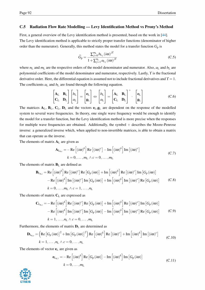
Page 92 Dissertation
C.5 Radiation Flow Rate Modelling — Levy Identification Method vs Prony’s Method
First, a general overview of the Levy identification method is presented, based on the work in [44].
The Levy identification method is applicable to strictly proper transfer functions (denominator of higher
order than the numerator). Generally, this method states the model for a transfer function Gp is
Gp =∑
mLj=0 bL j (iω) jϒ
1+∑nLj=1 aL j (iω) jϒ (C.5)
where nL and mL are the respective orders of the model denominator and numerator. Also, aL and bL are
polynomial coefficients of the model denominator and numerator, respectively. Lastly, ϒ is the fractional
derivative order. Here, the differential equation is assumed not to include fractional derivatives and ϒ= 1.
The coefficients aL and bL are found through the following equation.AL BL
CL DL
bL
aL
=
eL
gL
⇔bL
aL
=
AL BL
CL DL
+
·
eL
gL
(C.6)
The matrices AL, BL, CL, DL and the vectors eL,gL are dependent on the response of the modelled
system to several wave frequencies. In theory, one single wave frequency would be enough to identify
the model for a transfer function, but the Levy identification method is more precise when the responses
for multiple wave frequencies are obtained. Additionally, the symbol + describes the Moore-Penrose
inverse: a generalized inverse which, when applied to non-invertible matrices, is able to obtain a matrix
that can operate as the inverse.
The elements of matrix AL are given as
ALk,c =−Re[(iω)k
]Re[(iω)c]− Im
[(iω)k
]Im[(iω)c]
k = 0, . . . ,mL ∧ c = 0, . . . ,mL
(C.7)
The elements of matrix BL are defined as
BLk,c = Re[(iω)k
]Re[(iω)c]Re
[Gp (iω)
]+ Im
[(iω)k
]Re[(iω)c] Im
[Gp (iω)
]−Re
[(iω)k
]Im[(iω)c] Im
[Gp (iω)
]+ Im
[(iω)k
]Im[(iω)c]Re
[Gp (iω)
]k = 0, . . . ,mL ∧ c = 1, . . . ,nL
(C.8)
The elements of matrix CL are expressed as
CLk,c =−Re[(iω)k
]Re[(iω)c]Re
[Gp (iω)
]+ Im
[(iω)k
]Re[(iω)c] Im
[Gp (iω)
]−Re
[(iω)k
]Im[(iω)c] Im
[Gp (iω)
]− Im
[(iω)k
]Im[(iω)c]Re
[Gp (iω)
]k = 1, . . . ,nL ∧ c = 0, . . . ,mL
(C.9)
Furthermore, the elements of matrix DL are determined as
DLk,c =(
Re[Gp (iω)
]2+ Im
[Gp (iω)
]2)Re[(iω)k
]Re[(iω)c]+ Im
[(iω)k
]Im[(iω)c]
k = 1, . . . ,nL ∧ c = 0, . . . ,nL
(C.10)
The elements of vector eL are given as
eLk,1 =−Re[(iω)k
]Re[Gp (iω)
]− Im
[(iω)k
]Im[Gp (iω)
]k = 0, . . . ,mL
(C.11)

Air Turbine Rotational Speed Control of Oscillating-Water-Column Wave Energy Converters Page 93
Finally, the elements of vector gL are formulated as
gLk,1 =−Re[(iω)k
](Re[Gp (iω)
]2+ Im
[Gp (iω)
]2)k = 1, . . . ,nL
(C.12)
The model for the transfer function is presented in the form of a Bode diagram: a dual representation of
the gain and phase response for the total range of tested wave frequencies.
The model gain is given, in decibel, as
KL = 20log10
∣∣∣Gp (iω)∣∣∣ (C.13)
On the other hand, the model phase is expressed as
αL = tan−1
Im[Gp (iω)
]Re[Gp (iω)
] (C.14)
The objective of this annex is to define a model that approximates the transfer function of the linearized
uniform pressure model dynamics in equations (4.15) and (4.17), according to the Levy identification
method, in the real environment wave frequency range ω ∈ [0.45,1.43] rad/s [12].
The transfer function of the linearized uniform pressure model dynamics outputs the complex amplitude
of the radiation flow rate as a function of the complex amplitude of the excitation flow rate, which is the
input. It is formulated as
Gp =Qr
Qe=
Qr
Pc
Pc
Qe=−(G+ iH)
[KDρaΩ
+G+ i(
ωVc0
γ pa+H
)]−1
(C.15)
First, the Levy identification method is employed in the modelling of the Pico plant operating with the
original Wells turbine, of turbine geometry constant K = 0.6803 and diameter D = 2.3m. The gain,
phase and the roots’ placement of the obtained model are illustrated in figure C.5.
Figure C.5: Modelling of the Pico plant operating with the original Wells turbine through the Levyidentification method: model gain, phase and roots’ placement.

Page 94 Dissertation
The model was found to be of seventh order and its denominator and numerator are detailed in table C.6.
j aL [-] bL [-]0 0.3343 −0.35631 1.4030 −0.16232 1.9826 −0.96763 4.8076 −0.30924 3.2004 −0.53105 4.5197 −0.058636 1.3113 —7 1.000 —
Table C.6: Modelling of the Pico plant operating with the original Wells turbine through the Levyidentification method: model denominator and numerator.
Having obtained the model for the transfer function, integrated computer programming functions in the
utilized software are able to obtain the complex amplitude of the radiation flow rate as a model response
of the complex amplitude of the excitation flow rate input.
As in section 6.3, the pneumatic power available to the turbine relative root-mean-square error and corre-
lation coefficient error metrics are obtained for the comparison between the complex variable and linear
time domain analyses of the Pico plant operating with the original Wells turbine. The error metric results
for the computation of the radiation flow rate through the direct integration of equation (4.24), i.e., ana-
lytically, and through Prony’s method, in figures 6.5 and 6.6, are also displayed for comparison.
The numerical simulations are performed for regular waves of amplitude Aw = 1m and a turbine rota-
tional speed of Ω = 750rpm = 78.54rad/s. The studied wave frequency range is ω ∈ [0,2.5] rad/s, with
a wave frequency computational step of ωs = 0.01rad/s. Also, the computational time step is Ts = 0.1s.
Figure C.6 illustrates the relative root-mean-square error of the pneumatic power available to the turbine.
Figure C.6: Relative root-mean-square error of the pneumatic power available to the turbine for the Picoplant operating with the original Wells turbine: total (top) and real environment (bottom) wave frequencyrange. Comparison between all tested radiation flow rate modelling methods.
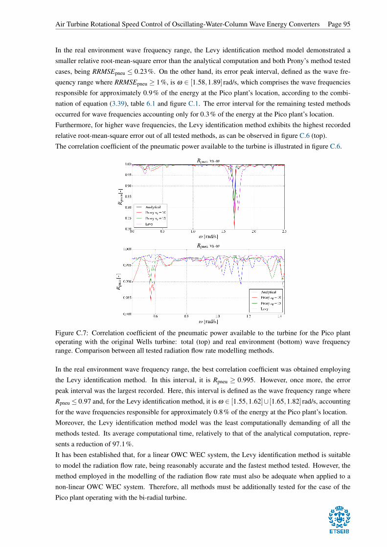
Air Turbine Rotational Speed Control of Oscillating-Water-Column Wave Energy Converters Page 95
In the real environment wave frequency range, the Levy identification method model demonstrated a
smaller relative root-mean-square error than the analytical computation and both Prony’s method tested
cases, being RRMSEpneu ≤ 0.23%. On the other hand, its error peak interval, defined as the wave fre-
quency range where RRMSEpneu ≥ 1%, is ω ∈ [1.58,1.89] rad/s, which comprises the wave frequencies
responsible for approximately 0.9% of the energy at the Pico plant’s location, according to the combi-
nation of equation (3.39), table 6.1 and figure C.1. The error interval for the remaining tested methods
occurred for wave frequencies accounting only for 0.3% of the energy at the Pico plant’s location.
Furthermore, for higher wave frequencies, the Levy identification method exhibits the highest recorded
relative root-mean-square error out of all tested methods, as can be observed in figure C.6 (top).
The correlation coefficient of the pneumatic power available to the turbine is illustrated in figure C.6.
Figure C.7: Correlation coefficient of the pneumatic power available to the turbine for the Pico plantoperating with the original Wells turbine: total (top) and real environment (bottom) wave frequencyrange. Comparison between all tested radiation flow rate modelling methods.
In the real environment wave frequency range, the best correlation coefficient was obtained employing
the Levy identification method. In this interval, it is Rpneu ≥ 0.995. However, once more, the error
peak interval was the largest recorded. Here, this interval is defined as the wave frequency range where
Rpneu ≤ 0.97 and, for the Levy identification method, it is ω ∈ [1.55,1.62]∪ [1.65,1.82] rad/s, accounting
for the wave frequencies responsible for approximately 0.8% of the energy at the Pico plant’s location.
Moreover, the Levy identification method model was the least computationally demanding of all the
methods tested. Its average computational time, relatively to that of the analytical computation, repre-
sents a reduction of 97.1%.
It has been established that, for a linear OWC WEC system, the Levy identification method is suitable
to model the radiation flow rate, being reasonably accurate and the fastest method tested. However, the
method employed in the modelling of the radiation flow rate must also be adequate when applied to a
non-linear OWC WEC system. Therefore, all methods must be additionally tested for the case of the
Pico plant operating with the bi-radial turbine.

Page 96 Dissertation
The Levy identification method presupposes turbine linearity and is therefore tested for the linearized
bi-radial turbine, described in annex C.3 (turbine geometry constant K = 0.12 and diameter D = 1.3m).
The gain, phase and the roots’ placement of the acquired model are illustrated in figure C.8.
Figure C.8: Modelling of the Pico plant operating with the linearized bi-radial turbine through the Levyidentification method: model gain, phase and roots’ placement.
Once more, the model was experimentally verified to be of seventh order. The model denominator and
numerator are presented in table C.7.
j aL[-] bL[-]0 0.0797 −0.15191 0.6714 −0.41182 0.6540 −0.54323 2.6873 −1.05694 1.3533 −0.44525 3.1781 −0.51216 0.7560 —7 1.000 —
Table C.7: Modelling of the Pico plant operating with the linearized bi-radial turbine through the Levyidentification method: model denominator and numerator.
In a non-linear OWC WEC system, the complex variable analysis is no longer applicable. Thus, to
compare the Levy identification method with Prony’s method, the relative root-mean-square error and
the correlation coefficient of the pneumatic power, respectively formulated in equations (6.2) and (6.3),
must be redefined.
First, the relative root-mean-square error of the pneumatic power available to the turbine is now given as
RRMSEpneu =
√1N ∑
j2j= j1
(PA
pneu j−PN
pneu j
)2
∑j2j= j1 PA
pneu j
(C.16)

Air Turbine Rotational Speed Control of Oscillating-Water-Column Wave Energy Converters Page 97
The correlation coefficient of the pneumatic power available to the turbine is, in this case, expressed as
Rpneu =∑
j2j= j1
(PA
pneu j−PA
pneuavg
)(PN
pneu j−PN
pneuavg
)√
∑j2j= j1
(PA
pneu j−PA
pneuavg
)2∑
j2j= j1
(PN
pneu j−PN
pneuavg
)2(C.17)
In equations (C.16) and (C.17), the time series for the pneumatic power available to the turbine calculated
with the non-linear time domain analysis is PApneu for the analytical computation of the radiation flow rate
and PNpneu for its approximation through either Prony’s method or the Levy identification method.
The numerical simulation conditions are identical to those of the previous experiment, except, in this
case, only the real environment wave frequency range is studied. The relative root-mean-square and the
correlation coefficient of the pneumatic power available to the turbine are illustrated in figure C.9.
Figure C.9: Relative root-mean-square error (top) and correlation coefficient (bottom) of the pneumaticpower available to the turbine for the Pico plant operating with the linearized bi-radial turbine in thereal environment wave frequency range. Comparison between all tested radiation flow rate modellingapproximation methods.
Testing Prony’s method and the Levy identification method in the numerical simulation of the Pico plant
operating with the bi-radial turbine, it was experimentally verified that the Levy identification method
exhibits the highest results for the tested error metrics, particularly concerning the correlation coefficient,
presented in figure C.9 (bottom). Overall, the results in figure C.9 indicate the Levy identification method
inadequately models the radiation flow rate for a non-linear OWC WEC system.
In the present work, the bi-radial turbine, which is distinctly non-linear, is tested. Hence, despite the
reasonable results obtained for the application of the Levy identification method for a linear OWC WEC
system, the better performance of Prony’s method in comparison with the Levy identification method
for a non-linear OWC WEC system means that, in this work, the application of Prony’s method is more
adequate when modelling the radiation flow rate.