air quality pattern assessment in malaysia using multivariate

Malaysian Journal of Analytical Sciences, Vol 19 No 5 (2015): 966 - 978

966

MALAYSIAN JOURNAL OF ANALYTICAL SCIENCES

Published by The Malaysian Analytical Sciences Society

AIR QUALITY PATTERN ASSESSMENT IN MALAYSIA USING

MULTIVARIATE TECHNIQUES

(Penilaian Corak Kualiti Udara di Malaysia Menggunakan Teknik Multivariat)

Hamza Ahmad Isiyaka and Azman Azid*

East Coast Environmental Research Institute (ESERI),

Universiti Sultan Zainal Abidin,

Gong Badak Campus, 21300 Kuala Terengganu, Terengganu, Malaysia

*Corresponding author: [email protected]

Received: 14 April 2015; Accepted: 9 July 2015

Abstract

This study aims to investigate the spatial characteristics in the pattern of air quality monitoring sites, identify the most

discriminating parameters contributing to air pollution, and predict the level of air pollution index (API) in Malaysia using

multivariate techniques. Five parameters observed for five years (2000-2004) were used. Hierarchical agglomerative cluster

analysis classified the five air quality monitoring sites into two independent groups based on the characteristics of activities in

the monitoring stations. Discriminate analysis for standard, backward stepwise and forward stepwise mode gave a correct

assignation of more than 87% in the confusion matrix. This result indicates that only three parameters (PM10, SO2 and NO2) with

a p<0.0001 discriminate best in polluting the air. The major possible sources of air pollution were identified using principal

component analysis that account for more than 58% and 60% in the total variance. Based on the findings, anthropogenic

activities (vehicular emission, industrial activities, construction sites, bush burning) have a strong influence in the source of air

pollution. Furthermore, artificial neural network (ANN) was used to predict the level of air pollution index at R2 = 0.8493 and

RMSE = 5.9184. This indicates that ANN can predict more than 84% of the API.

Keywords: multivariate techniques, principal component analysis, artificial neural network, air pollution index

Abstrak

Kajian ini adalah bertujuan untuk menyiasat ciri-ciri spatial dalam pemantauan corak kualiti udara, mengenal pasti parameter

yang menjadi penyumbang kepada pencemaran udara, dan meramalkan tahap indeks pencemaran udara (IPU) di Malaysia

menggunakan teknik multivariat. Lima parameter udara bagi lima tahun (2000-2004) telah digunakan. Hirarki algorithma analisa

kelompok telah mengkelaskan lima tapak pemantauan kualiti udara kepada dua kumpulan berdasarkan ciri-ciri aktiviti di stesen

pemantauan. Analisis pembezalayan bagi kaedah standard, langkah demi langkah ke belakang dan langkah demi langkah ke

hadapan memberikan peratusan yang dibenar lebih daripada 87% dalam matriks kekeliruan. Keputusan ini menunjukkan bahawa

hanya tiga parameter (PM10, SO2 dan NO2) dengan p<0,0001 memberikan pembezalayan yang baik dalam pencemaran di udara.

Sumber utama kemungkinan pencemaran udara telah dikenal pasti menggunakan analisis komponen utama yang menyumbang

lebih daripada 58% dan 60% dalam jumlah varians. Berdasarkan hasil kajian, aktiviti antropogenik (pelepasan kenderaan, aktiviti

perindustrian, tapak pembinaan, pembakaran belukar) mempunyai pengaruh yang kuat dalam sumber pencemaran udara.

Tambahan pula, rangkaian neural buatan (RNB) telah digunakan untuk meramal tahap indeks pencemaran udara dengan nilai R2

= 0.8493 dan RMSE = 5.9184. Ini menunjukkan bahawa RNB boleh meramalkan IPU lebih daripada 84%.

Kata kunci: teknik multivariate, analisis komponen utama, rangkaian neural buatan, indeks pencemaran udara

ISSN

1394 - 2506

Ahmad Isiyaka et al: AIR QUALITY PATTERN ASSESSMENT IN MALAYSIA USING MULTIVARIATE

TECHNIQUES

967

Introduction

Air is the most precious natural resources that sustain the existence of man, animals, plants as well as the general

ecosystem regulation. It is a mixture of gasses which serves as a spacesuit of the biosphere and held by the force of

gravity [1,2]. Air helps to retain heat that warms the earth surface, reduces temperature extremes between day and

night as well as absolve ultraviolet solar radiation [3]. The quality of air is determined by measuring the

concentration of gaseous pollutants and sizes or number of particulate matter emitted from natural or anthropogenic

sources [4]. Air is polluted when particulate toxic elements and gasses released into the atmosphere build up in

concentration sufficiently high to cause damage [5,6].

Atmospheric air pollution has adverse effect on the environment and health status of a given population. This is

because air is polluted from various sources and its complexity is largely dependent on the meteorological

characteristics, topography and the nature of the pollutants been emitted [7]. Rapid advancement in the level of

industrial activities and population concentration within the second half of the twentieth century poses a serious

threat to atmospheric air quality and well-being [8]. Furthermore, many accidental discharge of air pollutants results

in acute exposure and potential risk on human health [9].

Despite the effort put in place by both government and stakeholders to monitor and control air pollution level, its

negative and hazardous impact is enormous [10]. However, an estimate of the regional variability of air pollution

can be best understood taking into account the location of monitoring sites within a study area [11]. Atmospheric air

pollutants limits the amount of oxygen fed to the foetus through the mother when inhaled, thereby retarding the

anthropometric development of the child by reducing its head circumference [12]. It can also cause environmental

degradation (global warmining), lung cancer, asthma, cardiovascular and respiratory diseases [13,14].

API is used to identify and classify the ambient air quality in Malaysia base on the possible health implications to

the public [15]. It is a non-dimensional number calculated according to the urban daily average concentration of

pollutants [16,17]. API in Malaysia is calculated based on the sub-index using five air pollution parameters (PM10,

SO2, NO2, CO2 and O3). The highest sub-index value of the individual pollutants is used as the API value for a

specific time period [16,18,19]. This is based on the Recommended Malaysia Ambient Air Quality Guideline

(RMAQG) issued by the Department of Environment (DOE) since 1989 as; good, moderate, unhealthy, very

unhealthy and hazardous. Although, it conform to international standard as provided by United State Environmental

Protection Agency [19].

Atmospheric air quality monitoring involves observation of large complex data sets from stations that require the

integration of modern and robust statistical techniques for simplification, avoid misinterpretation and to show

spatial variation [20,21,22]. Several research has shown that the level of air pollution in Malaysia fall within the

range of good and moderate but still show a slight fluctuation in trend from 2008 to 2011 [17]. In 2008, the status of

good air quality fall around 59%, 55.6% in 2009, 63% in 2010 and 55% in 2011 [17].

The objectives of this study is to determine the spatial characteristics in the air quality monitoring sites, identify the

sources of pollution and the most discriminating parameters contributing to the air pollution, and predict the level of

air pollution index using artificial neural network.

Materials and Methods

Study Area

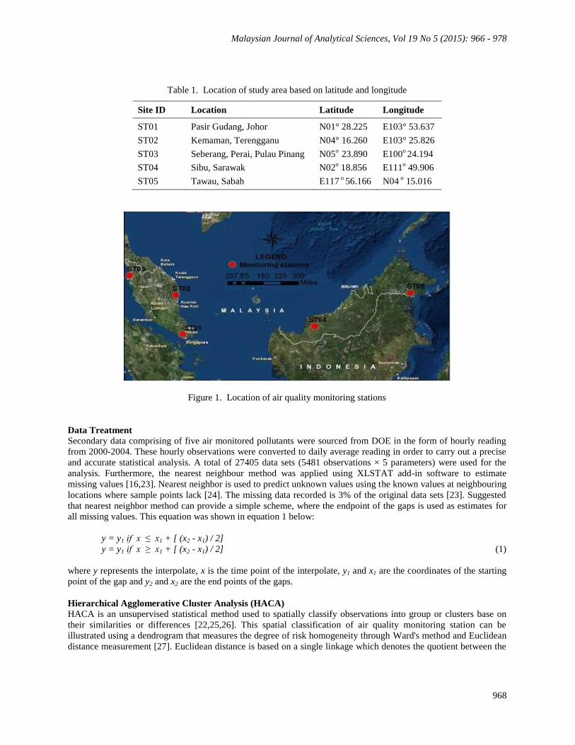
Five air quality monitoring sites were selected to give a general representation of the air quality status in Malaysia.

These five monitoring stations are under the supervision and control by a private company (Alam Sakitar Malaysia

Sdn. Bhd (ASMA) on behalf of Department of Environment Malaysia (DOE). The monitoring sites comprises of

Pasir Gudang, Johor (ST01) located in the southern Peninsular Malaysia; Kemaman, Terengganu (ST02) located in

the eastern Peninsular Malaysia; Perai, Pulau Pinang (ST03) in the Northern Peninsular Malaysia. Sibu Sarawak

(ST04) and Tawu Sabah (ST05) are situated in the eastern Malaysia. Furthermore, the location of the study area

base on their latitude and longitude are shown in Table 1 and Figure 1.


968

Table 1. Location of study area based on latitude and longitude

Site ID Location Latitude Longitude

ST01 Pasir Gudang, Johor N01° 28.225 E103° 53.637

ST02 Kemaman, Terengganu N04° 16.260 E103° 25.826

ST03 Seberang, Perai, Pulau Pinang N05o

23.890 E100o 24.194

ST04 Sibu, Sarawak N02o 18.856 E111

o 49.906

ST05 Tawau, Sabah E117 o

56.166 N04 o 15.016

Figure 1. Location of air quality monitoring stations

Data Treatment

Secondary data comprising of five air monitored pollutants were sourced from DOE in the form of hourly reading

from 2000-2004. These hourly observations were converted to daily average reading in order to carry out a precise

and accurate statistical analysis. A total of 27405 data sets (5481 observations × 5 parameters) were used for the

analysis. Furthermore, the nearest neighbour method was applied using XLSTAT add-in software to estimate

missing values [16,23]. Nearest neighbor is used to predict unknown values using the known values at neighbouring

locations where sample points lack [24]. The missing data recorded is 3% of the original data sets [23]. Suggested

that nearest neighbor method can provide a simple scheme, where the endpoint of the gaps is used as estimates for

all missing values. This equation was shown in equation 1 below:

y = y1 if x ≤ x1 + [ (x2 - x1) / 2]

y = y1 if x ≥ x1 + [ (x2 - x1) / 2] (1)

where y represents the interpolate, x is the time point of the interpolate, y1 and x1 are the coordinates of the starting

point of the gap and y2 and x2 are the end points of the gaps.

Hierarchical Agglomerative Cluster Analysis (HACA)

HACA is an unsupervised statistical method used to spatially classify observations into group or clusters base on

their similarities or differences [22,25,26]. This spatial classification of air quality monitoring station can be

illustrated using a dendrogram that measures the degree of risk homogeneity through Ward's method and Euclidean

distance measurement [27]. Euclidean distance is based on a single linkage which denotes the quotient between the


TECHNIQUES

969

linkage distance divided by the maximal distance [(Dlink/Dmax)], by multiplying the quotient by 100 in order to

standardize the linkage distance represented by the y-axis [28,29,30].

Discriminate Analysis (DA)

DA is usually applied in order to identify the variables that best discriminate between groups developed by HACA

and helps to construct new discriminant functions (DFs) for each group in order to evaluate the spatial variation in

atmospheric air quality [21,31].

DFs are calculated using Equation 2:

F (Gi) = Ki + ∑jn

=1 wij Pij (2)

where i = the number of group G; kj = constant inherent to each group; n = the number of parameters used to

classify a set of data into a given group; wj = the weight coefficient assigned by discriminant function analysis

(DFA) to a given parameter Pj,

In this study, DA is applied on the raw data for spatial analysis in the two clusters developed by HACA using

standard mode, backward stepwise mode and forward stepwise mode to determine whether the group differ with

regards to the mean of the variable and to use that variable to predict group membership. To achieve this, cluster 1

and 2 were selected as dependent variable, while the five monitored parameters represent the independent variables.

Using the forward stepwise mode, variables were included step by step from the most significant until no significant

changes are observed, while in the backward stepwise mode, variables were removed step by step beginning from

the less significant variable until no significant changes were observed [21].

Principal Component Analysis

PCA is the most used pattern recognition technique for analysing large and complex data sets [22]. It is used to

extract the most significant parameters by eliminating the less significant parameters with minimal loss of the

original variables [28,29,30].The equation is expressed as equation 3 below:

Zij = ai1x1j + ai2x2j+ ai3x3j +........... + aimxmj (3)

where z is the component score, a is the component loading, x is the measured value of variables, i is the component

number, j is the sample number and m is the total number of variables.

Although, the principal components (PCs) generated by PCA are sometimes not readily available for interpretation,

therefore, it is advisable to rotate it by varimax rotation with eigenvalues greater than 1 [21]. The varimax rotation is

considered significant in order to obtain new groups of variables called varimax factors (VFs) [32,33]. This will

help identify the different possible sources of pollution [18,24].

Furthermore, the number of varimax factors(VFs) obtained by varimax rotations is usually equal to the number of

variables in accordance with the common features which can include unobservable, hypothetical and latent variables

[34,35]. In addition, the VFs coefficient with a correlation from 0.75 are considered as strong significant factor

loading, those that range from 0.50 - 0.74 are moderate, while 0.30 - 0.49 are classified as weak significant factor

loading [36]. The equation is expressed as equation 4 below:

Zij = af1 x1i + af2 x2i + ........+ afm fmi + efi (4)

where Z is the measured value of a variables, a is the factor loading, f is the factor score, e is the residual term

accounting for errors or other sources variation, i is the sample number, j is the variable number and m is the total

number of factors.


970

Artificial Neural Network (ANN)

ANN is a distributed information processing system and powerful general purpose software composed of many

simple computational elements integrating across weighted connections [37]. It is a very sophisticated model used

for forecasting the concentration of pollutants and to estimating the level of air pollution index [38]. In this study, a

multilayer perceptron feed-forward artificial neural network (MLP-FF-ANN) was applied in order to predict the

level of air pollution index.

The network structure is designed to consist of multiple neurons organized in layers that enable information to flow

via an input system (independent variable). From the input layer signal is passed to the hidden layer via a system of

weighted connection where the actual processing is done and finally reached the output layer (dependent variable)

[39]. The network is trained severally by adjusting the weight value in order to minimize error and optimize the

number of hidden nodes in each layer [40]. To achieve this, a Backpropagation algorithm is introduced to the

network in order to correlate the coefficient between the expected and the calculated using a supervised learning

[40,41].

Furthermore, the coefficient of the determination (R2) and the root mean square error (RMSE) were used to evaluate

the result gotten in the ANN model. The higher the R2 with a low RMSE the better the prediction capabilities of the

ANN model [42]. The equation is written as equation 5 and 6:

𝑅2 = 1 −∑(𝑥𝑖−𝑦𝑖)2

∑ 𝑦𝑖2−

∑ 𝑦𝑖2

𝑛

(5)

𝑅𝑀𝑆𝐸 = √1

𝑛∑

𝑛

𝑖=1(𝑥𝑖 − 𝑦𝑖)

2 (6)

where xi represent the observed data, yi is the predicted data and n is the number of observation. The network

structure of MLP-FF-ANN is shown in Figure 2.

Figure 2. Network structure of MLP-FF-ANN model

Fiv

e in

pu

t Para

meters

API


TECHNIQUES

971

Results and Discussion

Spatial Classification of Air Monitoring Stations

The five air quality monitoring sites were spatially classified based on their level of differences and similarities in

the activities within the study area. Stations with high level of similarities were unsupervisely grouped into one

cluster. This resulted in the formation of two independent clusters in a dendrogram in Figure 3. Station 1, 2, 4 and 5

were successfully integrated into cluster 1, while station 3 stands independent from others as cluster 2.

Cluster 1 is classified as moderate polluted area (MPA) that is strongly associated with the nature of activities from

both point source and non-point source. These areas are characterized with commercial and industrial practices,

heavy traffic congestion, large scale forest fire from Sumatra (Indonesia) and airports [43,44]. Part of this area is the

extensively Rajan River in Borneo (Sarawak) with agricultural activities and a well-developed water transport

system [43]. This four stations exhibit a strong similarities in their characteristics.

Cluster 2 is classified as a residential area, tourist centre with little industrial activities [43,44]. This cluster can be

recognized as a less polluted area (LPA).

Figure 3. Spatial classification of the air monitoring sites

Discriminate Analysis (DA)

The most significant parameters that best discriminate spatially based on the clusters developed by HACA were

determined using standard mode, forward stepwise and backward stepwise DA. The two clusters were used as

dependent variables while the five monitored parameters were applied as the independent variables.

The result of the confusion matrix for standard, forward and backward stepwise mode gave a correct assignation of

over 87% indicating that only three parameters (PM10, SO2 and NO2) discriminate best with a p-value ˂0.0001. The

spatial classification matrix for DA is shown in Table 2.

Identification of The Major Possible Sources of Pollution

The spatial composition pattern of the examined parameters and sources of pollutants were identified using PCA.

For each cluster, two PCs were obtained with an eigenvalue greater than one. The cumulative variance gave a

correct assignation of more than 58% and 60% of the total variance in the data sets. In order to identify the most

significant parameters only factor loading greater than 0.7 were considered for interpretation. Table 3 and Figure 4

show the highlights of selected factors with strong positive loadings (˃0.7), eigenvalues greater than one (˃1) and

cumulative variance. The scree plot diagram for PCA loadings in Figure 5 indicates the cut-off point where strong

factors are selected for interpretation.


972

Table 2. Spatial classification matrix of DA based on clusters

Sampling Stations Regions % Correct

Cluster 1 Cluster 2

Standard mode

Cluster 1 4158 226 94.84%

Cluster 2 448 648 59.12%

Total 4606 874 87.70%

Forward stepwise mode

Cluster 1 4158 226 94.84%

Cluster 2 450 646 58.94%

Total 4608 872 87.66%

Backward stepwise

Mode

Cluster 1 4158 226 94.84%

Cluster 2 450 646 58.94%

Total 4608 872 87.66%

Cluster 1 The first varifactor (VF1) explains 38.4% of the total variance with a strong positive loading for PM10 (0.734) and

NO2 (0.862). Heavy industrial activities, emission from automobiles and aircrafts, Sumatra bush burning,

construction sites are the major sources of PM10 and NO2. Johor and Kemaman houses large industrial and

commercial activities [45]. Johor borders the Indonesia were most of the Sumatra bush burning come from. This

areas also experiences heavy traffic round the clock.

Table 3. Factor loading after varimax rotation based on clusters

Cluster 1 Cluster 2

Variables VF1 VF2 VF1 VF2

CO 0.423 0.115 0.608 -0.173

O3 -0.008 0.992 0.093 0.906

PM10 0.734 0.035 0.806 0.205

SO2 0.679 -0.047 0.622 -0.374

NO2 0.862 -0.018 0.741 0.18

Eigenvalue 1.922 1.001 1.966 1.062

Variability (%) 38.44 20.029 39.321 21.247

Cumulative % 38.44 58.469 39.321 60.567


TECHNIQUES

973

Figure 4. Factor loading plot after varimax rotation for cluster 1 and 2

Figure 5. Scree plot diagram for PCA loading in cluster 1 and 2

O3 (0.992) is the most significant parameter with a strong positive loadings in the second varifactor in cluster 1. It

accounts for over 20% of the total variance in the data set. Its formation is produced by photochemical oxidation

and act as the main component of photochemical smog [46]. The concentration of O3 is largely dependent on the

availability of its precursors (NOx, CO and VOCs), since O3 is a secondary pollutant. These precursors are from

industrial activities and vehicular emission [44,47].

Cluster 2

The second cluster exhibit a strong positive loading for PM10 (0.806) and NO2 (0.741) that explains over 39% in the

data set. Heavy construction activities and emissions from automobiles contribute immensely to PM10 emission.

[48,49]. PM10 are mostly emitted from heavy construction work for city development as well as resuspension of soil

and road dust. Large proportion of NO2 is produced when nitrogen in fuel is burnt and when at a very high

CO

O3

PM10 SO2 NO2

-1

-0.75

-0.5

-0.25

0

0.25

0.5

0.75

1

-1 -0.75 -0.5 -0.25 0 0.25 0.5 0.75 1

F2 (

20

.03

%)

Cluster 1 F1 (38.44 %)

Variables (axes F1 and F2: 58.47 %)

CO

O3

PM10

SO2

NO2

-1

-0.75

-0.5

-0.25

0

0.25

0.5

0.75

1

-1 -0.75 -0.5 -0.25 0 0.25 0.5 0.75 1

F2 (

21

.25

%)

Cluster 2 F1 (39.32 %)

Variables (axes F1 and F2: 60.57 %)

0

20

40

60

80

100

0

0.5

1

1.5

2

2.5

F1 F2 F3 F4 F5

Cu

mu

lati

ve v

aria

bili

ty (

%)

Eige

nva

lue

Cluster 1 axis

Scree plot

0

20

40

60

80

100

0

0.5

1

1.5

2

2.5

F1 F2 F3 F4 F5C

um

ula

tive

var

iab

ility

(%

)

Eige

nva

lue

Cluster 2 axis

Scree plot


974

temperature nitrogen in the air reacts with oxygen [50]. An estimate by [45] show that about 69% of NO2 is emitted

from power stations and industrial activities, 28% from motor vehicles and the remaining 3% makes up other

sources.

The second varifactor have a strong positive loading for O3 (0.906) which accounts for more than 21% of the total

variance in the data set. Its concentration is dependent on its precursors (NOx, CO and VOCs) from industrial and

motor vehicle emission [47].

Prediction of Air Pollution Index using ANN

Based on the coefficient of determination (R2) and root mean square error (RMSE) ANN was used to predict the

level of air pollution index. The network structure for the ANN model was run ten times in order to train the

network and to approximate any non-linear function with a high level of precision. However, the optimum gauge for

the ANN network where the best prediction is achieved was gotten at node six. Further optimization of the network

resulted in a decrease in the prediction capability of the MLP-FF-ANN. For training, the highest R2 = 0.8493 and

the lowest RMSE = 5.9184 was gotten at node six. The network was also validated at R2 = 0.8456 and RMSE =

6.1128.

Table 4 below show the prediction performance of the MLP-FF-ANN at different nodes based on R2 and RMSE.

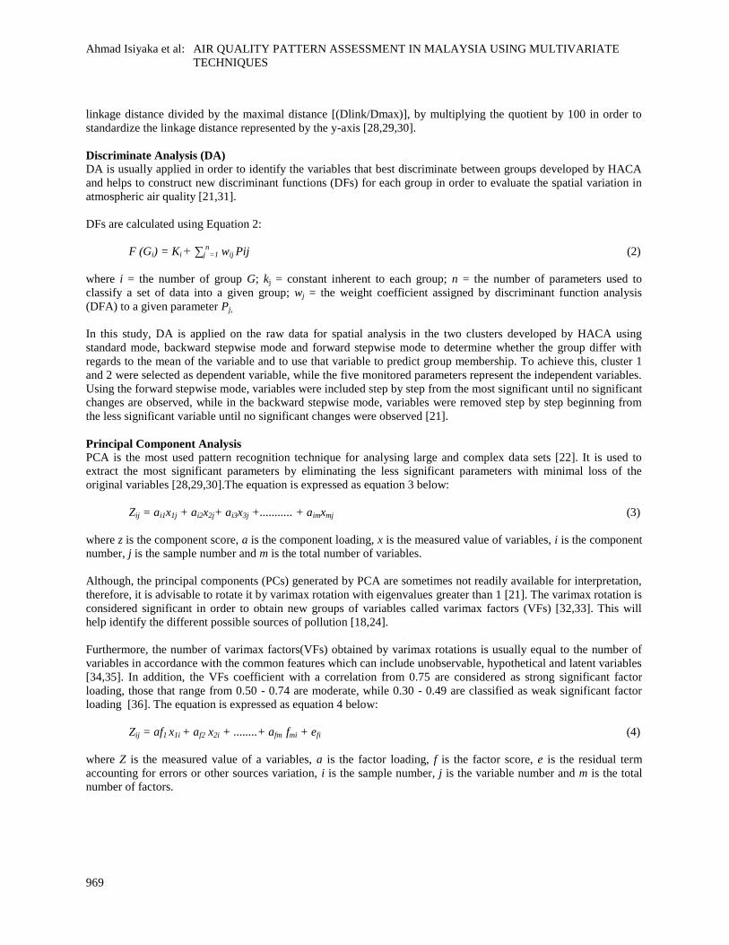
Figure 6 indicate the scatter plot for the training and validation phase of the MLP-FF-ANN. ANN is a sophisticated

software capable of predicting the concentration of pollutants as well as give an estimate in the level of air pollution

index [38]. It has the ability to learn complex pattern and can synthesise them better than conventional machines

[37].

Table 3. MLP-FF-ANN Performance Based on R2 and RMSE

Model

Training Validation

MLP-FF-ANN Hidden nodes R2 RMSE R

2 RMSE

[5,1,1] 0.8016 6.7909 0.7977 6.9970

[5,2,1] 0.8339 6.2122 0.8337 6.3440

[5,3,1] 0.8432 6.0308 0.8437 6.1501

[5,4,1] 0.8435 6.0308 0.8415 6.1935

[5,5,1] 0.8464 5.9755 0.8428 6.1684

[5,6,1] 0.8493 5.9184 0.8456 6.1128

[5,7,1] 0.8420 6.0594 0.8380 6.2621

[5,8,1] 0.8447 6.0080 0.8422 6.1795

[5,9,1] 0.8452 5.9973 0.8338 6.2466

[5,10,1] 0.8443 6.0148 0.8423 6.1772


TECHNIQUES

975

Figure 6. Scatter plots for (a) training and (b) validation phase for MLP-FF-ANN

Conclusion

The spatial variation in the characteristics of air pollution in Malaysia was assessed using multivariate techniques.

The five air quality monitoring stations were spatially grouped into two independent clusters using HACA. This

classification indicates strong similarities in the characteristics of monitoring sites in the same clusters. HACA

helps to minimize the number of monitoring sites that will directly or indirectly reduce the cost and time of

monitoring redundant stations. The result for DA in the entire data sets based on clusters developed by HACA gave

a correct assignation of more than 87% with P ˂0.0001 for only three parameters (PM10, SO2 and NO2). This clearly

indicates that the three primary and secondary pollutants discriminate best out of the five monitored parameters.

PCA explains 58% and 60% of the total variance in the data sets. The source of air pollution based on PCA loadings

after varimax rotation attributes it to heavy industrial activities, emission from automobiles, construction sites and

Sumatra bush burning (anthropogenic induced emission). MLP-FF-ANN was used to predict the level of air

pollution index with a very high precision. The result for training gave an R2 = 0.8493 and RMSE = 5.9184, while

the network was validated at R2 = 0.8456 and RMSE = 6.1128 at node six.


976

Acknowledgement

The author wish to extend his profound gratitude to the Department of Environment Malaysia for providing the data

used for this study. East Coast Environmental Research Institute (ESERI), Universiti Sultan Zainal Abidin,

Malaysia is highly appreciated for the wonderful assistance it provided in putting this work to reality.

References

1. Yazdanpanah, H., Karimi, M. and Hejazizadeh, Z. (2009). Forecasting of daily total atmospheric ozone in

Isfahan Environmental Monitoring Assessment 157:235–241.

2. Botkin, D. B., Keller, E. A., and Rosenthal, D. B. (2012). Environmental Science. Wiley.

3. Brunekreef, B. and Holgate, S. T. (2002). Air pollution and health. The lancet 360 (9341): 1233-1242.

4. World Health Organization (2002). World Health Report: Reducing Risk, Promoting Healthy Life. Geneva,

Switzerland.

5. Jacobson, M. Z. (2002). Atmospheric pollution: history, science, and regulation. Cambridge University Press.

6. Bernstein, J. A., Alexis, N., Barnes, C., Bernstein, I. L., Nel, A., Peden, D. and Williams, P. B. (2004). Health

effects of air pollution. Journal of Allergy and Clinical Immunology 114(5): 1116-1123.

7. De-Souza, A., Aristones, F., Pavão, H. G., and Fernandes, W. A. (2014). Development of a Short-Term Ozone

Prediction Tool in Campo Grande-MS-Brazil Area Based on Meteorological Variables. Open Journal of Air

Pollution 3(02): 42-51.

8. Ramanathan, V. and Feng, Y. (2009). Air pollution, greenhouse gases and climate change: Global and regional

perspectives. Atmospheric Environment 43(1): 37-50.

9. Department of Environment Malaysia (DOE) (2007). Malaysia Environmental Quality Report, Ministry of

Science, Technology and Environment, Kuala Lumpur.

10. Zell, H., Quarcoo, D., Scutaru, C., Vitzthum, K., Uibel, S., Schöffel, N. Mache, S., Groneberg, D.A and

Spallek, M. F. (2010). Research Air pollution research: visualization of research activity using density-

equalizing mapping and scientometric benchmarking procedures. Journal of Occupational Medicine and

Toxicology 5(5): 1-9.

11. Turalıoğlu, F. S., Nuhoğlu, A. and Bayraktar, H. (2005). Impacts of some meteorological parameters on SO2

and TSP concentrations in Erzurum, Turkey. Chemosphere 59(11): 1633-1642.

12. Ballester, F., Llop, S., Estarlich, M., Esplugues, A., Rebagliato, M. and Iñiguez, C. (2010). Preterm birth and

exposure to air pollutants during pregnancy. Environmental Research 110(8):778-785.

13. Ilyas, S. Z., Khattak, A. I., Nasir, S. M., Qurashi, T. and Durrani, R. (2010). Air pollution assessment in urban

areas and its impact on human health in the city of Quetta, Pakistan. Clean Technologies and Environmental

Policy 12(3): 291-299.

14. MacNee, W. and Donaldson, K. (2003). Mechanism of lung injury caused by PM10 and ultrafine particles with

special reference to COPD. European Respiratory Journal 21(40): 47s-51s.

15. Department of Environment Malaysia (DOE) (1997). A Guide to Air Pollution Index In Malaysia (API).

Ministry of Science, Technology and Environment, Kuala Lumpur.

16. Dominick, D., Juahir, H., Latif, M. T., Zain, S. M., & Aris, A. Z. (2012). Spatial assessment of air quality

patterns in Malaysia using multivariate analysis. Atmospheric Environment, 60, 172-181.



18. Mutalib, S. N. S. A., Juahir, H., Azid, A., Sharif, S. M., Latif, M. T., Aris, A. Z., Zain, S. M. and Dominick,D.,

(2013). Spatial and temporal air quality pattern recognition using environmetric techniques: a case study in

Malaysia. Environmental Science, Processes & Impacts 15(9): 1717-1728.

19. Wu, E.M. and Kuo, S. (2013). A study of the use of a statistical analysis model to monitor air pollution status in

an air quality-total control district. Atmosphere 4: 349-364

20. Samsudin, M. S., Juahir, H., Zain, S. M. and Adnan, N. H. (2011). Surface river water quality interpretation

using environmetric techniques: Case study at Perlis River Basin, Malaysia. International Journal of

Environmental Protection 1(5): 1-8.

21. Juahir, H., Zain, S. M., Yusoff, M. K., Hanidza, T. T., Armi, A. M., Toriman, M. E. and Mokhtar, M. (2011).

Spatial water quality assessment of Langat River Basin (Malaysia) using environmetric techniques.

Environmental Monitoring and Assessment 173(1-4): 625-641.


TECHNIQUES

977

22. Al-Odaini, N. A., Zakaria, M. P., Zali, M. A., Juahir, H., Yaziz, M. I., & Surif, S. (2012). Application of

chemometrics in understanding the spatial distribution of human pharmaceuticals in surface water.

Environmental Monitoring And Assessment 184(11), 6735-6748.

23. Junninen, H., Niska, H., Tuppurainen, K., Ruuskanen, J. and Kolehmainen, M. (2004). Methods for imputation

of missing values in air quality data sets. Atmospheric Environment 38(18), 2895-2907.

24. Azid, A., Juahir, H., Toriman, M. E., Kamarudin, M. K. A., Saudi, A. S. M., Hasnam, C. N. C., Abdul Aziz, N.

A., Azaman, F., Latif, M. T., Zainuddin, S. F. M., Osman, M. R. and Yamin, M. (2014). Prediction of the Level

of Air Pollution Using Principal Component Analysis and Artificial Neural Network Techniques: a Case Study

in Malaysia. Water, Air, & Soil Pollution, 225(8): 2063 – 2077.

25. Farmaki, E. G, Thomaidis, N. S, Simeonov, V. and Efstathiou, C. E. (2012). A comparative chemometric study

for water quality expertise of the Athenian water reservoirs Environmental Monitoring Assessment 184:7635 –

7652.

26. Zhang, X., Jiang, H. and Zhang, Y. (2013). Spatial distribution and source identification of persistent pollutants

in marine sediments of Hong Kong. Environmental Monitoring Assessment 185: 4693-4704.

27. Lau, J., Hung, W.T. and Cheung, C.S. (2009). Interpretation of air quality in relation to monitoring station’s

surrounding. Atmospheric Environmetric 43: 769-777

28. Singh, K. P., Malik, A., Mohan, D. and Sinha, S. (2004). Multivariate statistical techniques for the evaluation of

spatial and temporal variations in water quality of Gomti River (India)—a case study. Water Research, 38(18):

3980-3992.

29. Singh, K.P., Malik, A. and Sinha, S. (2005) Water quality assessment and apportionment of pollution sources

of Gomti River (India) using multivariate statistical techniques a case study. Analytica Chimica Acta 538: 355-

374.

30. Shrestha, S. and Kazama, F. (2007). Assessment of surface water quality using multivariate statistical

techniques: A case study of the Fuji river basin, Japan. Environmental Modelling & Software 22(4): 464-475.

31. Pati, S., Dash, M. K., Mukherjee, C. K., Dash, B. and Pokhrel, S. (2014). Assessment of water quality using

multivariate statistical techniques in the coastal region of Visakhapatnam, India. Environmental Monitoring and

Assessment 186(10): 6385-6402.

32. Brūmelis, G., Lapiņa, L., Nikodemus, O. and Tabors, G. (2000). Use of an artificial model of monitoring data

to aid interpretation of principal component analysis. Environmental Modelling & Software 15(8):755-763.

33. Love, D., Hallbauer, D., Amos, A. and Hranova, R. (2004). Factor analysis as a tool in groundwater quality

management: two southern African case studies. Physics and Chemistry of the Earth, Parts A/B/C 29(15):

1135-1143.

34. Vega, M., Pardo, R., Barrado, E. and Debán, L. (1998). Assessment of seasonal and polluting effects on the

quality of river water by exploratory data analysis. Water Research, 32(12): 3581-3592.

35. Helena, B., Pardo, R., Vega, M., Barrado, E., Fernandez, J. M. and Fernandez, L. (2000). Temporal evolution

of groundwater composition in an alluvial aquifer (Pisuerga River, Spain) by principal component analysis.

Water Research 34(3): 807-816.

36. Liu, C. W., Lin, K. H. and Kuo, Y. M. (2003). Application of factor analysis in the assessment of groundwater

quality in a blackfoot disease area in Taiwan. Science of the Total Environment 313(1): 77-89.

37. Hakimpoor, H., Arshad, K. A. B., Tat, H. H., Khani, N. and Rahmandoust, M. (2011). Artificial neural

networks’ applications in management. World Applied Sciences Journal 14 (7): 1008-1019.

38. Moustris, K. P., Larissi, I. K., Nastos, P. T., Koukouletsos, K. V. and Paliatsos, A. G. (2013). Development and

Application of Artificial Neural Network Modeling in Forecasting PM10 Levels in a Mediterranean City.

Water, Air, & Soil Pollution 224(8):1-11.

39. Dongare, A. D., Kharde, R. R. and Kachare, A. D. (2012). Introduction to artificial neural network.

International Journal of Engineering and Innovative Technology (IJEIT) 2: 189-194.

40. Arhami, M., Kamali, N. and Rajabi, M. M. (2013). Predicting hourly air pollutant levels using artificial neural

networks coupled with uncertainty analysis by Monte Carlo simulations. Environmental Science and Pollution

Research 20(7), 4777-4789.

41. Juahir, H., Zain, S., Md., Aris A.Z., Mazlin, M., K. Y. and Mokhtar, B. (2009). Spatial assessment of Langat

river Water quality using chemometrics. Journal of Environmental Monitoring 12: 287–295.

42. Sarkar, A. and Kumar, R. (2012). Artificial Neural Networks for Event Based Rainfall-Runoff Modeling.

Journal of Water Resource and Protection 4(10): 891-897.


978



44. Department of Statistic Malaysia (DOS) (2010). Basic Population Characteristics by Administrative Districts

2009 Report.



46. Banan, N., Latif, M. T., Juneng, L. and Ahamad, F. (2013). Characteristics of surface ozone concentrations at

stations with different backgrounds in the Malaysian Peninsula. Aerosol and Air Quality Research 13(3): 1090-

1106.

47. Sadanaga, Y., Sengen, M., Takenaka, N. and Bandow, H. (2012). Analyses of the ozone weekend effect in

Tokyo, Japan: regime of oxidant (O3+ NO2) production. Aerosol Air Quality Research 12: 161-168.

48. Abdullah, A. M., Abu Samah, M. A., and Jun, T. Y. (2012). An overview of the air pollution trend in Klang

Valley, Malaysia. Open Environ Science 6:13-19.

49. Sara, Y. Y., Rashid, M., Chuah, T. G., Suhaimi, M. and Mohamed, N. N. (2013). Characteristics of Airborne

PM2.5 and PM2.5-10 in the Urban Environment of Kuala Lumpur. In Advanced Materials Research 620: 502-

510.

50. Brunekreef, B. and Holgate, S. T. (2002). Air pollution and health. The Lancet 360(9341):1233-1242.

Documents

air quality pattern assessment in malaysia using multivariate