Air-quality implications of widespread adoption of cool

Air-quality implications of widespread adoption ofcool roofs on ozone and particulate matter insouthern CaliforniaScott A. Epsteina,1, Sang-Mi Leea, Aaron S. Katzensteina, Marc Carreras-Sospedraa, Xinqiu Zhanga, Salvatore C. Farinaa,Pouya Vahmanib, Philip M. Finea, and George Ban-Weissb

aPlanning, Rules, and Area Sources Division, South Coast Air Quality Management District, Diamond Bar, CA 91765; and bSonny Astani Department of Civiland Environmental Engineering, University of Southern California, Los Angeles, CA 90089

Edited by Christopher B. Field, Stanford University, Stanford, CA, and approved July 5, 2017 (received for review March 8, 2017)

The installation of roofing materials with increased solar reflec-tance (i.e., “cool roofs”) can mitigate the urban heat island effectand reduce energy use. In addition, meteorological changes, alongwith the possibility of enhanced UV reflection from these surfaces,can have complex impacts on ozone and PM2.5 concentrations. Weaim to evaluate the air-quality impacts of widespread cool-roofinstallations prescribed by California’s Title 24 building energy ef-ficiency standards within the heavily populated and pollutedSouth Coast Air Basin (SoCAB). Development of a comprehensiverooftop area database and evaluation of spectral reflectance mea-surements of roofing materials allows us to project potential fu-ture changes in solar and UV reflectance for simulations using theWeather Research Forecast and Community Multiscale Air Quality(CMAQ) models. 2012 meteorological simulations indicate a de-crease in daily maximum temperatures, daily maximum boundarylayer heights, and ventilation coefficients throughout the SoCABupon widespread installation of cool roofs. CMAQ simulationsshow significant increases in PM2.5 concentrations and policy-relevant design values. Changes in 8-h ozone concentrations de-pend on the potential change in UV reflectance, ranging from adecrease in population-weighted concentrations when UV reflec-tance remains unchanged to an increase when changes in UV re-flectance are at an upper bound. However, 8-h policy-relevantozone design values increase in all cases. Although the other ben-efits of cool roofs could outweigh small air-quality penalties, UVreflectance standards for cool roofing materials could mitigatethese negative consequences. Results of this study motivate thecareful consideration of future rooftop and pavement solar reflec-tance modification policies.

urban air quality | albedo | California Title 24 | Los Angeles |urban surface modification

The South Coast Air Basin (SoCAB) is a region of southernCalifornia encompassing Orange County and the urban por-

tions of Los Angeles, San Bernardino, and Riverside counties.With 16.8 million people, the SoCAB is the second most popu-lous urban area in the United States. A fossil-fuel-dependenttransit and goods movement infrastructure along with a well-developed industrial presence within the 27,824-km2 SoCABgenerates significant emissions of oxides of nitrogen (NOx), volatileorganic compounds (VOCs), directly emitted primary particulatematter (PM), and secondary PM precursors. Persistent high-pressure systems, ample photochemistry, infrequent rainfall, andventilation-inhibiting topography also contribute to severe air-quality problems. The SoCAB currently does not attain federalair-quality standards for 8-h O3, 1-h O3, annual-averaged PM2.5,and 24-h PM2.5. Ozone levels within the SoCAB are often thehighest in the nation (1).The hot and sunny conditions typically experienced within the

SoCAB make urban surface modification a useful strategy toreduce urban temperatures. Meteorological impacts of roofingmaterials with enhanced solar reflectance (SR, synonymous with

“albedo”), colloquially referred to as “cool roofs,” are well-studied and indicate several benefits in urban areas. The re-placement of darker materials with high-reflectance surfaceswithin cities can help mitigate the urban heat island effect (2–14).Moreover, meteorological modeling suggests that the deploymentof cool roofs will reduce afternoon summertime temperatures,leading to reduced cooling energy demands, resulting in a cur-tailment of greenhouse gas emissions (15, 16) in most urban areas.Cool roofs will also lower the Earth’s radiative forcing by in-creasing the global albedo (17–19), although impacts on globalclimate remain unsettled in the literature (20), with recent re-search suggesting effects are negligible (4).Cool roofs can affect air quality through several mechanisms,

although there are far fewer studies investigating these effectscompared with the wealth of meteorological and climatologicalstudies. Because the air-quality effects of urban surface modifi-cation by cool roofs are complex and nonlinear, comprehensiveemissions processing, meteorological, and chemical transportmodels are needed to accurately determine potential impacts onair quality for policy-making purposes. Potential changes inmixing height and ventilation (21) will affect ambient pollutantconcentrations. Cool roofs can reduce temperature-dependentemissions of precursors to O3 and PM in urban areas by lower-ing ambient temperatures, resulting in a slower rate of VOCevaporation and NOx emissions (14). In addition, the atmosphericreactions that produce O3 are slower at lower temperatures. A

Significance

The South Coast Air Basin of California, a region of 16.8 millionpeople, is among the most polluted air basins in the UnitedStates. A multidecadal effort to attain federal air-qualitystandards has led to significant progress, but much morework remains. Are recently implemented statewide buildingefficiency standards on rooftops counterproductive to thesegoals? With comprehensive regional models and intensive de-velopment of model input parameters, our research has iden-tified the air-quality consequences that are expected to resultfrom these efficiency standards. The results can inform policiesto mitigate some air-quality penalties, while preserving thebenefits of building efficiency standards. This work also shedslight on potential future policies aimed at reducing urbanheating from pavement surfaces.

Author contributions: S.A.E., S.-M.L., A.S.K., P.M.F., and G.B.-W. designed research; S.A.E.,M.C.-S., X.Z., S.C.F., P.V., and G.B.-W. performed research; S.A.E. and S.C.F. contributednew reagents/analytic tools; S.A.E. and G.B.-W. analyzed data; and S.A.E. and G.B.-W.wrote the paper.

The authors declare no conflict of interest.

This article is a PNAS Direct Submission.1To whom correspondence should be addressed. Email: [email protected].

This article contains supporting information online at www.pnas.org/lookup/suppl/doi:10.1073/pnas.1703560114/-/DCSupplemental.

www.pnas.org/cgi/doi/10.1073/pnas.1703560114 PNAS Early Edition | 1 of 6

EART

H,A

TMOSP

HER

IC,

ANDPL

ANET

ARY

SCIENCE

SSU

STAINABILITY

SCIENCE

http://crossmark.crossref.org/dialog/?doi=10.1073/pnas.1703560114&domain=pdf&date_stamp=2017-08-02

mailto:[email protected]

http://www.pnas.org/lookup/suppl/doi:10.1073/pnas.1703560114/-/DCSupplemental

http://www.pnas.org/lookup/suppl/doi:10.1073/pnas.1703560114/-/DCSupplemental

www.pnas.org/cgi/doi/10.1073/pnas.1703560114

handful of studies modeled the effect of cool-roof installationson O3 concentrations during short-term multiday O3 episodes inthe SoCAB (22–26). Population-weighted O3 exposures werereduced with an increase in urban SR; however, O3 concentra-tions in the less-populated eastern SoCAB exhibited O3 in-creases. Further increases in surface SR led to smaller netreductions in O3 because significant weakening of the sea breezeled to reduced vertical mixing.To the authors’ knowledge, all but one (29) of the previous

studies investigating the role of cool-roof materials on air qualityassume that widespread adoption of cool roofs will not changeUV reflectance (UVR) (2, 22–27). Increases in UVR can signif-icantly affect photochemical production of O3. For example, O3concentrations in the Uintah Basin are elevated in the winterduring periods of snow cover due to increased UV reflectivity andlimited mixing from reduced surface heating (28). Fallmann et al.(29) modified building SR for all urban grid cells in Stuttgard,Germany from 0.2 to 0.7 across all wavelengths. Although thisincrease in UVR is unrealistically high, the authors saw a signif-icant increase in peak O3 concentrations during a clear-sky, sunnyperiod, which they attribute to increases in reflected UV radiation.In this research effort we aim to rigorously evaluate the air-

quality effects in the SoCAB of current cool-roof installation poli-cies in California Title 24 Building Energy Efficiency Standards(Title24) (30). Besides O3, we also focus on PM2.5 concentrations, apollutant that largely drives the health impacts of air pollution insouthern California (31) and whose link to cool-roof adoption is notwidely studied. With newly analyzed data on the UVR of hundredsof real-world roofing products, we directly evaluate the assumptionused in previous studies that standard and cool roofs have nearlythe same UVR and then probe the sensitivity of UVR on result-ing pollutant concentrations. Rather than focusing on specificair-pollution episodes, we have conducted a collection of com-prehensive simulations over an entire calendar year. We developeda high-resolution database of building rooftop areas classified byland-use category to project future SR after full implementation ofTitle24 standards in the SoCAB. WRF v3.6, a state-of-the-sciencemeteorological model, was used to forecast changes in meteorologyinduced by cool roofs. The temperature-dependent 2012 SoCABemissions inventory (1) and a modified version of the state-of-the-science Community Multiscale Air Quality Model (CMAQ version5.0.2) were then used to project future O3 and PM2.5 concentrationsafter cool-roof implementation.

Materials and MethodsProjecting Future SR. Determining the effects of Title24 standards on SR re-quires information on the current SR and the total rooftop area in eachTitle24 building category. Title24 standards prescribe that new or renovatedrooftops meet SR standards that are based on climate zone (SI Appendix, Fig.S1) and building type (30) (Table 1). We determined the rooftop area of eachTitle24 building category in every model grid cell with land-use data for2012 from the Southern California Association of Governments (SCAG) andbuilding footprint data from the US Army Corps of Engineers (32). SeeSI Appendix.

We used monthly Moderate Resolution Imaging Spectroradiometer(MODIS) measurements of SR (33) to determine base-case values for each4-km model grid cell. The current SR of rooftops for each Title24 category inthe SoCAB was calculated by combining recent aircraft-based remote sens-ing measurements of rooftops in Los Angeles and Long Beach, CA (8, 9) withSCAG land-use data (Table 1). The projected future building SR, set by theTitle24 standards, along with the current building SR, calculated with theremote sensing measurement data, allowed us to determine the expectedchange in SR in the fraction of each grid cell occupied by buildings anddetermine the monthly SR for each grid cell if all rooftops meet Title24standards. Fig. 1A details the calculated change in grid-cell average SR inresponse to full implementation of Title24 standards.

Projecting UVR for Chemical Transport Modeling. Photolysis reactions arewavelength-dependent (34); therefore, capturing changes in photochemis-try from Title24 requires careful consideration of wavelength-dependentreflectances. In situ remote sensing measurements of rooftop UVR are notavailable. However, several studies measured the wavelength-dependentspectral reflectance of roofing materials (8, 9, 35–37). To bound the possi-ble change in wavelength-dependent reflectance, Fig. 2 presents spectralreflectance measurements (8, 9) for a wide variety of traditional and cool roof

Table 1. Current and future SR values corresponding to Title24 categories

Title24 category Climate zones Current SR* Title24 SR SoCAB area†, km2 Title24 area‡, km2

Nonresidential low slope All 23 63 262.3 262.3Nonresidential high slope All 19 20 96.5 96.5High-rise low slope residential, hotel, and motel 9–11, 13–15 20 55 16.1 7.6High-rise high slope residential, hotel, and motel 2–15 14 20 21.7 21.5Residential low slope 13–15 20 63 67.2 0.7Residential high slope 10–15 14 20 580.3 150.6

*Calculated from remote sensing measurements in Los Angeles and Long Beach (11, 12), which were applied to all climate zones.†This is the area of each Title24 land-use category in the SoCAB.‡This is the area of each Title24 land-use category in the SoCAB that is in a climate zone affected by Title24 standards.

A

Sol

ar R

efle

ctan

ce (

Titl

e24-

Bas

elin

e)

0

0.02

0.04

0.06

0.08

B

UV

Ref

lect

ance

(T

itle2

4-B

asel

ine)

0

0.005

0.01

0.015

0.02

0.025

Fig. 1. (A) Change in SR (Title24 – baseline) used for WRF simulations. (B)Maximum possible change in UVR (Title24 – baseline) used for CMAQ simulations.

2 of 6 | www.pnas.org/cgi/doi/10.1073/pnas.1703560114 Epstein et al.

http://www.pnas.org/lookup/suppl/doi:10.1073/pnas.1703560114/-/DCSupplemental/pnas.1703560114.sapp.pdf




materials as a function of wavelength for high slope (Fig. 2A) and low slope(Fig. 2B) roofing materials (SI Appendix, Table S2). We define cool roofs, basedon Title24 standards, as those with an SR above 0.20 and 0.63 for low-slopeand high-slope roofing materials, respectively. To serve as an extreme upper-bound increase in UVR, we set the maximum change in reflectance at eachCMAQ wavelength range to be the largest difference between the cool andstandard roofing materials (Fig. 1B) and applied these differences to each ofthe Title24 categories based on their corresponding area in each grid cell.Projection of UVR is discussed more comprehensively in the SI Appendix. Wealso explored the scenario where UVR does not change to serve as a lowerbound. Each of these scenarios was used to drive photochemistry in theTitle24 simulations in CMAQ. The Title24 SR changes as derived in the pre-vious paragraph were used for the 410- to 850-nm wavelength band in theCMAQ simulations.

Emissions Processing. On-road NOx and VOC along with biogenic VOCemissions profiles are dependent on meteorology. Annual hourly emissionsprofiles were developed as a function of the baseline and Title24 meteo-rological fields for the 2012 base year. The SoCAB emissions inventory ispresented in ref. 1 and details of the emissions processing are presented inref. 38. Changes in NOx and VOC emissions in the baseline and Title24simulations are small, mainly due to the similarity in the meteorologicalfields. Within the SoCAB, on average during the O3 season, VOC emissionsare reduced by 0.1% (0.75 tons per day) and NOx emissions are reduced by8 × 10−4% (0.004 tons per day) in the Title24 scenario.

Within the SoCAB, changes in power-generation emissions are expected tobe insignificant with the widespread implementation of cool roofs and arenot accounted for in themodeling. Emissions from power generation are onlyresponsible for 0.4% of the total NOx emissions in the 2012 emission in-ventory. Additionally, only 37%of the total electricity consumed is generatedwithin the SoCAB (1).

Meteorological and Chemical Transport Modeling. WRF version 3.6.1 was usedwith a North American Regional Reanalysis field to simulate 2012 meteo-rology on three nested grids, with an inner 4-km grid covering the modelingdomain (SI Appendix, Fig. S9). (Details of the model setup are available inref. 38.) WRF model performance is summarized in SI Appendix, Figs. S10–

S19. Two year-long simulations were performed: a base case using theMODIS-derived SR fields and a Title24 case using the modified SR fieldsdetailed above assuming that all buildings in the SoCAB meet Title24 roof-top SR requirements.

CMAQ version 5.0.2 was used to simulate air quality without dynamiccoupling within a 624- × 408-km modeling domain on a 4-km grid with18 vertical layers. Extensive details of the modeling protocol are presented inref. 38. Modification of the CMAQ code allowed us to calculate spatiallyresolved photolysis rate constants based on wavelength-dependent re-flectance fields. As with any modeling study, results are dependent on themodel accurately capturing the physical and chemical processes under in-vestigation. SI Appendix, Figs. S20–S28 summarize the ability of CMAQ topredict measured concentrations of O3 and PM2.5 throughout the SoCAB.

Changes in annual averaged PM2.5, daily maximum 8-h O3, and dailymaximum 1-h O3 concentrations were evaluated across the modeling do-main. Student’s t tests for paired samples were conducted to determinewhether changes in concentration across different scenarios were statisti-cally significant. Differences with P values less than 0.05 were assumed to bestatistically significant.

To evaluate the impact of widespread cool-roof installation toward at-tainment of federal ambient air-quality standards, relative response factorprojections were also conducted to calculate changes in design values (DV).This strategy uses the ratio of Title24 vs. baseline concentrations to adjustmeasured values, cancelling out many of the systematic uncertainties re-sponsible for concentration biases. This analysis is consistent with Environ-mental Protection Agency (EPA) modeling guidance (39) and is presented inref. 38 with a summary in SI Appendix. Data and scripts, with minor exclu-sions (SI Appendix), are available with a South Coast Air Quality Manage-ment District public records request.

Results and DiscussionChanges in Meteorology. WRF simulations of 2012 meteorologyrepresenting the baseline (MODIS-derived SR) and Title24 (SRmodified for cool-roof adoption) cases are summarized in Fig. 3.Annual averaged daily high temperatures are projected to de-crease throughout the SoCAB (Fig. 3A) with the largest de-creases (∼0.35 K) in areas with the largest change in SR.Changes in the daily maximum planetary boundary layer height(PBLH) (Fig. 3B) are negative; the mixed layer height will de-crease by 40–65 m in the most polluted areas of the SoCAB inthe Title24 scenario, a significant difference compared withmodel-predicted average daily maximum mixed layer heights of1–2 km. A decrease in surface temperature can reduce thebuoyancy of the surface air, leading to a reduction in verticalmixing. Lower surface temperatures on land decrease the land–sea temperature gradient, slowing down the daytime sea breeze—an important mechanism that drives relatively clean marine airinto the SoCAB. The average of the 9 AM-to-3 AM ventilationcoefficient (VC), the integral of the horizontal wind velocitywith respect to height at all layers below the maximum mixingdepth (40) (Fig. 3C), decreases throughout the SoCAB withimplementation of Title24. Daily profiles of the change inseveral meteorological variables are presented in SI Appendix,Figs. S29–S32.

Changes in PM2.5 Concentrations. Several year-long CMAQ simu-lations were conducted to determine the individual effects ofchanges in meteorology, emissions, enhanced SR, and a range ofhypothetical changes in UVR. Fig. 4A shows the change in an-nual PM2.5 concentrations between the baseline simulation(scenario I in Table 2) and a simulation using Title24 meteo-rology, emissions resulting from the Title24 meteorology, andthe assumption that UVR does not increase (scenario IV). Av-erage PM2.5 concentrations increase throughout the SoCAB,presumably caused by reductions in mixing heights and VCs, aswell as partitioning of semivolatile species to the particle phaseat lower temperatures. In the populated central Los Angelesregion and Long Beach, annual PM2.5 concentrations are pro-jected to increase by approximately 0.3 μg·m−3. Fig. 4B illustratesthe change in the number of days that exceed the 24-h PM2.5standard of 35 μg·m−3 (scenario IV – scenario I). These changes

A

B

Fig. 2. Range of wavelength-dependent reflectance of cool and standardroofing materials for high-slope (A) and low-slope (B) applications.

Epstein et al. PNAS Early Edition | 3 of 6

EART

H,A

TMOSP

HER

IC,

ANDPL

ANET

ARY

SCIENCE

SSU

STAINABILITY

SCIENCE














are location-dependent, with increases in Los Angeles and theInland Empire where PM2.5 is typically highest.Changes in annual averaged PM2.5 at the Mira Loma moni-

toring location—the most polluted PM2.5 station in the SoCAB—for each simulation are presented in Table 2. Implementation ofTitle24 emissions (scenario III) does not affect PM2.5 concen-trations relative to the baseline scenario (scenario I). However,the inclusion of Title24 meteorology (scenario IV) leads to anannual average PM2.5 increase of 0.19 ± 0.007 μg·m−3. Increasesin UVR (scenario V) lead to minimal changes in PM2.5

concentrations.Changes in SoCAB maximum annual and 24-h PM2.5 policy-

relevant DVs calculated with the EPA-recommended relativeresponse factor approach are also shown in Table 2. SoCABmaximum annual DVs are expected to increase by approximately0.2 μg·m−3 even if increases in UVR are avoided—importantcompared with the 12 μg·m−3 federal standards. Twenty-four-hour PM2.5 DVs are projected to increase by 0.62–0.65 μg·m−3

depending on changes in UVR—important compared with the24-h PM2.5 standard of 35 μg·m−3.

Changes in Ozone Concentrations. Fig. 5 shows changes in dailymaximum 8-h O3 (DM8HO3) concentrations averaged over theO3 season (May 1–September 30) for two scenarios. Fig. 5Ashows the changes expected if Title24 were fully implementedbut UVR was held constant (scenario IV – scenario I). O3concentrations largely decrease throughout the SoCAB, with theexception of the Redlands area, which typically experiences thehighest O3 concentrations in the SoCAB. However, most resi-dents in the SoCAB live in areas that will experience a decreasein O3 under this scenario. Whereas the number of 75 ppb exceed-ance days is relatively unchanged in the most populated areas of theSoCAB, the number of exceedance days increase in the regionsurrounding Redlands (SI Appendix, Fig. S35A). Fig. 5B showschanges in O3 concentrations resulting from an upper-boundchange in UVR (scenario V – scenario I). Increases in averageDM8HO3 concentrations are expected in most of the SoCAB inthis scenario (Fig. 5B). This translates to large increases in thenumber of exceedance days throughout the SoCAB (SI Appendix,Fig. S35A).Table 2 details changes in mean +/− standard error (SE)

DM8HO3 concentrations at Redlands, the station with thehighest 8-h O3 DV. Changes in 1-h averaged daily maximum O3(DM1HO3) concentrations are presented for Fontana, themonitoring station with the highest 1-h DVs in the SoCAB.Ozone concentrations are neither sensitive to increases in visibleand IR reflectance (scenario II) within CMAQ nor to decreasesin emissions inherent in the Title24 scenario (scenario III). Simu-lations with Title24 meteorology produce increases in averagedDM8HO3 concentrations (scenarios IV and V). Depending on

A

-0.35

-0.3

-0.25

-0.2

-0.15

-0.1

-0.05

0

Ann

ual A

vg. D

aily

Max

. T [K

]

B

-60

-50

-40

-30

-20

-10

0

10

Ann

ual A

vg. D

aily

Max

. PB

LH [m

]

C

-6

-4

-2

0

2

Ann

ual A

vg. (

9AM

-3P

M) V

C [%

]

Fig. 3. (A) Change in annual average daily max temperatures (Title24 –

baseline). (B) Change in annual average daily maximum PBLH. (C) Change inannual average VC calculated between 9 AM and 3 PM. Gray hashed cellsindicate that differences are not statistically significant (P > 0.05).

A

-0.1

0

0.1

0.2

0.3

PM

2.5

[g/

m3

]B

-2

-1

0

1

2

Day

s

Fig. 4. (A) Change in annual average PM2.5 concentrations (scenario IV –

scenario 1). The green circle indicates the location of the highest annualPM2.5 measured DVs in the basin. Seasonal differences in PM2.5 are presentedin SI Appendix, Fig. S34. (B) Change in the number of 24-h PM2.5 federalstandard (35 μg·m−3) exceedance days in a year (scenario IV – scenario 1).Gray hashed cells indicate that differences are not statistically significant(P > 0.05). Image represents 3- × 3-cell moving average.







the magnitude of UVR increases, DM8HO3 concentrations areprojected to increase by 0.04 ± 0.013 (scenario IV) to 0.66 ±0.015 ppb (scenario V), whereas DM1HO3 concentrations areprojected to change by −0.040 ± 0.023 to 0.96 ± 0.026 ppb.Although the increase in UVR in the upper-bound case is rela-tively small, ranging from 0 to 0.027 depending on location (Fig.1B), ozone formation is still extremely sensitive to these in-creases. The projected changes in SoCAB-maximum DVs for 8-hand 1-h O3 are presented in Table 2. Changes in O3 concen-trations and DVs are linearly dependent on the degree of UVRincreases (SI Appendix, Fig. S33 and Table S1). The SoCABmaximum 8-h DV increases by 0.3 ppb with a constant UVRacross the domain to 1.3 ppb with the UVR at the upper bound.Behavior of the 1-h SoCAB maximum DV is more complex. Ifincreases in UVR can be avoided, the 1-h DV is expected todecrease by 0.4 ppb. However, if concentrations are simulatedwith maximum increases in UVR, 1-h O3 DV concentrations canincrease by 1.9 ppb. This counterintuitive behavior can beexplained partially with Fig. 5. Fontana is further west thanRedlands and is in the region where O3 concentrations decreasewhen UVR is held constant and increase when UVR is at itsmaximum value. This illustrates the competition between themany factors governing O3 concentrations that can change withcool-roof implementation.

Policy Implications. Attainment of the 75-ppb 8-h O3 standard by2031 in the SoCAB is an extremely challenging air-quality goal,requiring an additional 55% reduction in NOx emissions beyondall existing regulations (1). Compliance with Title24 cool-roofstandards may make attainment of this goal more difficult, evenif future UVR increases are small. Scenario V assumes thatbuildings adopt cool roofing products with increase in UVR at anextreme upper bound. The actual increases in UVR throughoutthe SoCAB will depend on the individual roofing products that arechosen for installation. Although more realistic UVR increasescannot be projected without knowledge of the individual coolroofing products that are adopted, our analysis indicates thatUVR will likely increase when replacing standard roofs with coolroofs. Whether ozone ultimately increases or decreases in the mostpopulated areas of the basin will depend on the relative importanceof multiple physicochemical pathways, including ozone decreasesfrom temperature reductions, ozone increases from reducedventilation and mixing, and ozone increases from possible UVRincreases. Different magnitudes of SR increase or UVR increasemay change the dominating mechanisms. We also simulated 2031DVs with the presence of full Title24 implementation and fullimplementation of the proposed South Coast Air Quality

Management District control strategy (1). We estimate thateven if UVR increases can be entirely avoided, Title24 couldincrease the 2031 8-h DV by 0.3 ppb and the 2031 1-h DV by1.1 ppb. These increases in O3 concentrations are consequentialin light of the cost to reduce precursor emissions to achieve acorresponding reduction in O3 concentrations.Implementation of Title24 standards was used as the basis for

this analysis; however, several factors may influence futureadoption of cool roofs. Municipalities such as Los Angeles andPasadena have cool-roof ordinances that can lead to increases inSR beyond what would be expected with the Title24 standards.

Table 2. Simulated changes in PM2.5 and O3 at polluted locations

Scenarioname WRF SR Emissions

Reflectanceused to drivechemistry

Δ Annualaverage PM2.5

at Mira Loma,μg·m−3

Δ Dailymaximum 8-hO3 at Redlands,

ppb

Δ Dailymaximum 1-hO3 at Fontana,

ppb

Δ Basinmaximum

annual PM2.5

DV, μg·m−3

Δ Basinmaximum24-h PM2.5

DV, μg·m−3

Δ Basinmaximum8-h O3 DV,

ppb

Δ Basinmaximum1-h O3 DV,

ppb

I Baseline Baseline Baseline 0 0 0 0 0 0 0II Baseline Baseline Enhanced vis/IR,

no UV increase0.00 ± 0.000** 0.00 ± 0.000** 0.01 ± 0.000** 0 0 0 0

III Baseline Title24 Enhanced vis/IR,no UV increase

0.00 ± 0.000** −0.01 ± 0.000** −0.01 ± 0.001** 0 −0.07 0 0

IV Title24 Title24 Enhanced vis/IR,no UV increase

0.19 ± 0.007** 0.04 ± 0.013** −0.040 ± 0.023* +0.23 +0.62 +0.3 −0.4

V Title24 Title24 Enhanced vis/IR,maximum UVincrease

0.20 ± 0.008** 0.66 ± 0.015** 0.96 ± 0.026** +0.22 +0.65 +1.3 +1.9

Average concentrations are reported as nine cell averages (cell including station + eight adjacent cells). Uncertainty ranges represent the standard error.Δ indicates that the results of the baseline scenario were subtracted from the scenario indicated on each row. An additional scenario where UVR is increasedto one-half of its maximum value is presented in SI Appendix, Table S2. *P = 0.004; **P < 0.0001.

A

-0.5

0

0.5

1

O3

[ppb

]B

-0.5

0

0.5

1 O

3 [p

pb]

Fig. 5. (A) Change in annual average DM8HO3 values (scenario IV) with theassumption that UVR does not change with widespread installation of coolroofs. The green circle indicates the location of the highest 8-h O3 measuredDVs in the basin. (B) Change in annual average DM8HO3 values with the as-sumption that UVR increases are consistent with the maximum possible in-crease based on roofing products currently available (scenario V). Gray hashedcells indicate that differences are not statistically significant (P > 0.05).Image represents 3- × 3-cell moving average.

Epstein et al. PNAS Early Edition | 5 of 6

EART

H,A

TMOSP

HER

IC,

ANDPL

ANET

ARY

SCIENCE

SSU

STAINABILITY

SCIENCE



In addition, widespread adoption of solar photovoltaics andTitle24 cool-roof installation exemptions for the implementationof equivalent energy savings measures could also affect futurechanges in urban reflectance.The O3 concentration sensitivity to small changes in cool-roof

UVR supports the establishment of a standard regulating theUVR of certified cool-roof materials. Currently, materials mustmeet specific SR standards for consideration as a cool-roof ma-terial. Establishment of an additional UV standard could helpminimize inadvertent increases in O3. Furthermore, it is possiblethat a reduction in UVR below current values will lead to im-provements in O3 air quality throughout the SoCAB; this may bea cost-effective O3 control strategy. Remote sensing measure-ments of the current rooftop stock to survey UVR could help setstandards such that cool-roof materials do not lead to increasesin UVR when they replace existing rooftops.When assessing the impacts of cool roofs, it is important to

consider all environmental and economic consequences. Forexample, benefits from a reduction in heat-related mortality mayoutweigh the increase in mortality from enhanced PM2.5 pollu-tion. Also, widespread increases in urban SR can help to combatthe local impacts of climate change. Potential energy bill savings arealso an important benefit. In addition, there are other mechanisms

to control ambient air pollution such as emission reductions,whereas tools for mitigation of the urban heat island effect aremore limited. Without a comprehensive analysis of all of thebenefits of cool roofs it would be a mistake to discourage thistechnology solely on the basis of air quality alone.Relatively small changes in surface reflectance lead to signif-

icant impacts in O3 and PM2.5. Results of this analysis also shedlight on the choice of pavement materials and cool pavements, apotentially more important driver of overall urban SR and UVR.Analysis of impervious surface area (41) along with the rooftoparea database developed for this paper indicates that there issignificantly more pavement area in the SoCAB than rooftoparea (1,900 km2 of pavement area vs. 1,040 km2 of rooftop area).(SI Appendix, Fig. S36 presents the spatial distribution of pave-ment area throughout the SoCAB.) In addition, only a fractionof the total rooftop area was modified for projections of air qualitybecause Title24 does not affect rooftops in every climate zone.Therefore, the SR and UVR of pavements may be an importantdriver of regional air quality and human exposure to UV radiationand should be considered when evaluating cool pavement materials.

ACKNOWLEDGMENTS. This work was funded in part by NSF Grant CBET-1512429 (to G.B.-W.).

1. South Coast Air Quality Management District (2016) Final 2016 air quality managementplan (South Coast Air Quality Management District, Diamond Bar, CA).

2. Akbari H, Pomerantz M, Taha H (2001) Cool surfaces and shade trees to reduce energyuse and improve air quality in urban areas. Sol Energy 70:295–310.

3. Vahmani P, Sun F, Hall A, Ban-Weiss G (2016) Investigating the climate impacts ofurbanization and the potential for cool roofs to counter future climate change inSouthern California. Environ Res Lett 11:124027.

4. Zhang J, Zhang K, Liu J, Ban-Weiss G (2016) Revisiting the climate impacts of coolroofs around the globe using an Earth system model. Environ Res Lett 11:084014.

5. Stone B, Jr, et al. (2014) Avoided heat-related mortality through climate adaptationstrategies in three US cities. PLoS One 9:e100852.

6. Georgescu M, Morefield PE, Bierwagen BG, Weaver CP (2014) Urban adaptation canroll back warming of emerging megapolitan regions. Proc Natl Acad Sci USA 111:2909–2914.

7. Santamouris M (2014) Cooling the cities: A review of reflective and green roof miti-gation technologies to fight heat island and improve comfort in urban environments.Sol Energy 103:682–703.

8. Ban-Weiss GA, Woods J, Levinson R (2015) Using remote sensing to quantify albedo ofroofs in seven California cities, part 1: Methods. Sol Energy 115:777–790.

9. Ban-Weiss GA, Woods J, Millstein D, Levinson R (2015) Using remote sensing toquantify albedo of roofs in seven California cities, part 2: Results and application toclimate modeling. Sol Energy 115:791–805.

10. Li D, Bou-Zeid E, Oppenheimer M (2014) The effectiveness of cool and green roofs asurban heat island mitigation strategies. Environ Res Lett 9:055002.

11. Doulos L, Santamouris M, Livada I (2004) Passive cooling of outdoor urban spaces. Therole of materials. Sol Energy 77:231–249.

12. Santamouris M, Synnefa A, Karlessi T (2011) Using advanced cool materials in theurban built environment to mitigate heat islands and improve thermal comfortconditions. Sol Energy 85:3085–3102.

13. Li D, Bou-Zeid E (2013) Synergistic interactions between urban heat islands and heatwaves: The impact in cities is larger than the sum of its parts. J Appl Meteorol Climatol52:2051–2064.

14. Millstein D, Menon S (2011) Regional climate consequences of large-scale cool roofand photovoltaic array deployment. Environ Res Lett 6:034001.

15. Akbari H, Levinson R (2008) Evolution of cool-roof standards in the US. Adv BuildEnergy Res 2:1–32.

16. Levinson R, Akbari H (2009) Potential benefits of cool roofs on commercial buildings:Conserving energy, saving money, and reducing emission of greenhouse gases and airpollutants. Energy Effic 3:53–109.

17. Menon S, Akbari H, Mahanama S, Sednev I, Levinson R (2010) Radiative forcing andtemperature response to changes in urban albedos and associated CO2 offsets.Environ Res Lett 5:014005.

18. Akbari H, Menon S, Rosenfeld A (2009) Global cooling: Increasing world-wide urbanalbedos to offset CO2. Clim Change 94:275–286.

19. Akbari H, Matthews HD, Seto D (2012) The long-term effect of increasing the albedoof urban areas. Environ Res Lett 7:024004.

20. Jacobson MZ, Ten Hoeve JE (2011) Effects of urban surfaces and white roofs on globaland regional climate. J Clim 25:1028–1044.

21. Sharma A, et al. (2016) Green and cool roofs to mitigate urban heat island effects inthe Chicago metropolitan area: Evaluation with a regional climate model. Environ ResLett 11:064004.

22. Taha H (2008) Meso-urban meteorological and photochemical modeling of heat is-land mitigation. Atmos Environ 42:8795–8809.

23. Taha H (2015) Meteorological, air-quality, and emission-equivalence impacts of urbanheat island control in California. Sustainable Cities and Soc 19:207–221.

24. Taha H (2009) Urban surface modification as a potential ozone air-quality im-provement strategy in California–Phase Two: Fine-resolution meteorological andphotochemical modeling of urban heat islands (Altostratus Inc., Martinez, CA), ReportCEC-500-2009-071.

25. Taha H (2008) Urban surface modification as a potential ozone air-quality improve-ment strategy in California: A mesoscale modelling study. Boundary Layer Meteorol127:219–239.

26. Taha H (1997) Modeling the impacts of large-scale albedo changes on ozone airquality in the South Coast Air Basin. Atmos Environ 31:1667–1676.

27. Taha H (2005) Urban surface modification as a potential ozone air-quality improve-ment strategy in California–Phase One: Initial mesoscale modeling (Altostratus Inc.,Martinez, CA), Report CEC-500-2005-128.

28. Edwards PM, et al. (2014) High winter ozone pollution from carbonyl photolysis in anoil and gas basin. Nature 514:351–354.

29. Fallmann J, Forkel R, Emeis S (2016) Secondary effects of urban heat island mitigationmeasures on air quality. Atmos Environ 125:199–211.

30. California Energy Commission (2012) Building energy efficiency standards for residentialand nonresidential buildings. Title 24 Part 6 and associated administrative regulationsin Part 1 (California Energy Commission, Sacramento, CA).

31. South Coast Air Quality Management District (2016) Final socioeconomic report 2016 airquality management plan (South Coast Air Quality Management District, DiamondBar, CA).

32. Building Vectors, ed, Geospatial Repository and Data Management System (GRiD)Cold Regions Research and Engineering Laboratory (CRREL) Engineer Research andDevelopment Center (ERDC) (US Army Corps of Engineers, Washington, DC).

33. Vahmani P, Ban-Weiss GA (2016) Impact of remotely sensed albedo and vegetationfraction on simulation of urban climate in WRF-urban canopy model: A case study ofthe urban heat island in Los Angeles. J Geophys Res Atmos 121:1511–1531.

34. Finlayson-Pitts BJ, Pitts JN, Jr (2000) Chemistry of the Upper and Lower Atmosphere(Academic, San Diego).

35. Parker DS, McIlvaine JER, Barkaszi SF, Beal DJ, Anello MT (2000) Laboratory testing ofthe reflectance properties of roofing material (Florida Solar Energy Center, Cocoa, FL).

36. Prado RTA, Ferreira FL (2005) Measurement of albedo and analysis of its influence thesurface temperature of building roof materials. Energy Build 37:295–300.

37. Berdahl P, Bretz SE (1997) Preliminary survey of the solar reflectance of cool roofingmaterials. Energy Build 25:149–158.

38. South Coast Air Quality Management District (2016) Final 2016 air quality managementplan appendix V: Modeling and attainment demonstrations (South Coast Air QualityManagement District, Diamond Bar, CA).

39. US Environmental Protection Agency (2014) Draft modeling guidance for demonstratingattainment of air quality goals for ozone, PM2.5, and regional haze (US EnvironmentalProtection Agency, Washington, DC).

40. Ashrafi K, Shafie-Pour M, Kamalan H (2009) Estimating temporal and seasonal vari-ation of ventilation coefficients. Int J Environ Res 3:637–644.

41. Xian G, et al. (2011) Change of impervious surface area between 2001 and 2006 in theconterminous United States. Photogramm Eng Remote Sensing 77:758–762.




Supporting Information Appendix

Air Quality Implications of Widespread Adoption of Cool

Roofs on Ozone and Particulate Matter in Southern

California

Scott A. Epstein1, Sang-Mi Lee1, Aaron S. Katzenstein1, Marc Carreras-Sospedra1, Xinqiu Zhang1,

Salvatore Farina1, Pouya Vahmani2, Philip M. Fine1, and George Ban-Weiss2

1South Coast Air Quality Management District

Planning, Rules, and Area Sources Division

21865 Copley Drive

Diamond Bar, CA 91765-4178

2Sonny Astani Department of Civil and Environmental Engineering

University of Southern California

3620 S. Vermont Avenue, KAP 210

Los Angeles, CA 90089-2531

Corresponding Author: Scott A. Epstein, 21865 Copley Drive, Diamond Bar CA 91765-4178,

[email protected]

mailto:[email protected]

Supporting Information Appendix 2

SI Materials and Methods

Development of Building Footprint Database

With Southern California Association of Governments (SCAG) land use categories(1) and US

Army Corps of Engineers building footprint data (containing rooftop perimeters and average

rooftop slope), it was possible to determine the area of buildings in each of the six Title24

categories in each grid cell. However, interpolation was necessary to determine the rooftop

area in grid cells without building footprint data (Figure S2). Building area was not interpolated

directly. Instead, we interpolated two somewhat smoothly varying parameters: the plan area

fraction and the fraction of low slope buildings. While the interpolation introduces some

uncertainty, the majority of rooftop area in the SoCAB is explicitly defined in the datasets and

does not come from interpolated parameters.

First, SCAG land use categories were translated to Title24 categories. The parcel area in each

category was determined in each grid cell (Figure S3) without regard for building slope. The

area of buildings lying within each of these three Title24 land use categories could then be

tallied (Figure S4). However, since the US Army Corps of Engineers data does not cover the

entire SoCAB, we were only able to initially calculate building area for the regions covered by

the dataset. Next, we calculated the plan area fraction—defined as the area occupied by

buildings normalized by the entire parcel area in each of the three Title24 land use categories

(Figure S5 upper panes). Since the plan area fraction is somewhat of a smooth function

throughout the Basin, it was reasonable to interpolate this field using a natural neighbor

interpolation scheme to calculate the plan area fraction in grid cells without building footprint

data (Figure S5 lower panes). Cells with actual data were not replaced by the interpolated

fields. The building footprint data was then processed such that each building was tagged as

either low-slope or high-slope. This data could then be integrated with the land use data to

determine the low-slope fraction (area of low slope rooftops / total building area) in each of the

three Title24 land use categories (Figure S6 upper panes). This low-slope fraction was then

interpolated to fill in the missing grid cells (Figure S6 lower panes). As in the plan area fraction

interpolation, cells with actual data were not replaced by the interpolated fields. The plan area

fraction fields, the low-slope fraction fields, and the land use fields could then be combined to

determine the rooftop area in each of the six Title24 categories throughout the entire Basin

(Figure S7).

Projection of UVR for CMAQ Modeling

Unlike solar reflectance (SR), UV reflectance (UVR) measurements of the current building stock

are not available. Therefore, we designed a method to project future UVR to represent an

extreme upper-bound case. The methodology implemented for the analysis is detailed in the


main manuscript and shown as a schematic in Figure S8. However, there are other methods to

estimate future UVR under an extreme upper-bound case. Fortunately, our conclusions are not

highly sensitive to exactly where this upper-bound is established. The upper-bound CMAQ

simulations should not be interpreted as a likely future scenario; the results of these

simulations establish that between the lower-bound UVR projection case (UVR remains

unchanged in the future) and the upper-bound UVR projection case, ozone concentrations are

sensitive to changes in UVR and increase as UVR increases. The overall sensitivity of ozone

concentrations to UVR changes is linear in the region of the SoCAB with the highest ozone

concentrations (Figure S33) and can be used to estimate ozone with more realistic changes in

UVR.

We explored another extreme upper-bound UVR projection methodology to test the sensitivity

of our UVR projection. In this methodology, roofing materials with reflectance measurements

are grouped in the same fashion as detailed in the main document to represent high-slope cool

materials, high-slope standard materials, low-slope cool materials, and low-slope standard

materials. For each roofing material, the ratio of reflectance within a specific wavelength range

is normalized by the visible reflectance of that material (UVR/SR). A single high-UVR material is

selected to represent the high-slope cool materials by identifying the product that has the

highest normalized reflectance ratio (UVR/SR) in the first five UV wavelength bands (290nm-

300nm, 300nm-310nm, 310nm-315nm, 315nm-320nm, and 320nm-345nm). A single low-UVR

material is selected to represent the low-slope standard materials by identifying the product

that has the lowest normalized reflectance ratio in the first five UV wavelength bands. In the

same fashion, a single high-UVR material and a single low-UVR material were selected to

represent low-slope cool materials and low-slope standard materials, respectively. In order to

calculate the base-case UVR at each wavelength range, the reflectance ratios of the two

identified low-slope and high-slope standard products were multiplied by the current SR in each

land-use category from remote sensing measurements (See Table 1). In the same fashion, the

reflectance ratios of the two cool products were multiplied by the corresponding Title24

projected SR to estimate the upper-bound Title24 UVR at each wavelength range for each land-

use category. Upper-bound projected wavelength-dependent changes in reflectance for

rooftops in each land-use category could then be calculated by subtracting the corresponding

cool UVR from the corresponding standard UVR. The analogous values were calculated for the

high-slope materials. These upper-bound projected changes in wavelength dependent UVR

could then be weighted by the fraction of each Title24 land-use category in each grid-cell as

performed for the methodology detailed in the manuscript. This strategy produces upper-

bound UVR values that are slightly higher than the upper-bound UVR values calculated with the

original methodology in the first four wavelength bands where photons have the most energy

to induce photochemistry. Upper-bound UVR values calculated from this methodology are

slightly lower than the upper-bound UVR values calculated with the original methodology in the

two lower energy UV wavelength bands.


Calculation of Design Values and Relative Response Factor Based Projections

Design values are used to determine attainment of the National Ambient Air Quality

Standards as outlined in the United States Clean Air Act. 8-hour ozone, 1-hour ozone, 24-hour

average PM2.5 and annual average PM2.5 design values were calculated. 8-hour ozone design

values are based on the fourth highest daily maximum eight-hour averaged concentration

throughout the ozone season. These 8-hour values are averaged over a three year period. 1-

hour ozone design values are based on the fourth highest one-hour daily maximum ozone

concentration in a three year period. Annual average PM2.5 design values are based on the

average of all the daily PM2.5 concentrations while 24-hour averaged PM2.5 design values are

based on the 98th percentile highest-concentration day in a year. In order to minimize the

effects of year-to-year variations in meteorology and/or emissions, three adjacent three-year

design values are then averaged to generate five-year weighted design values. Moreover,

design values for 2012, the base-year of our simulations, incorporates measurement data from

2010 to 2014 with the most weight assigned to 2012 and the least weight assigned to 2010 and

2014. To evaluate changes in policy-relevant design values, a relative response factor (RRF)

approach is used to project baseline 2012 5-year weighted design values (2, 3). RRFs capture

the ratio of Title24 and baseline concentrations. The 8-hour ozone RRFs are based on the ratio

of daily-maximum concentrations on the days with the top 10 highest concentrations in the

baseline simulations. The 1-hour ozone RRFs use the ratio of daily -maximum concentrations

on the days with the top three highest concentrations in the baseline simulations. Design

values for the “Title24” simulations are the product of the baseline design values and the RRFs

at each measurement location. The annual RRFs are species specific (nitrate, sulfate, organic

carbon, elemental carbon, crustal material, salt, and ammonium) and are based on the average

of quarterly averaged concentrations in the baseline and Title24 simulations. These species

specific RRFs are then applied to the specific design values at each measurement location.

Annual PM2.5 design values for the “Title24” simulations are the sum of the product of each

species’ baseline design value and RRF.

Data Sharing

All data used in the paper is available publicly via a South Coast Air Quality Management District

public records request with the following restrictions:

Raw building footprint data used to build the database of buildings in the South Coast

Air Basin were acquired form the US Army Corps of Engineers. We are unable to share

this data as it is labeled "for official use only." The processed product used for the

meteorological and air quality modeling is available.

Roof manufacturer and model names for products measured and reported in Figure 2

cannot be shared with the public, but the spectral reflectance data is available.


References

1. 2012 Regional Transportation Plan/Sustainable Communities Strategy. (Southern California Association of Governments, Los Angeles, CA).

2. Final 2016 Air Quality Management Plan Appendix V: Modeling and Attainment Demonstrations. (South Coast Air Quality Management District, Diamond Bar, CA).

3. U.S. Environmental Protection Agency (2014) Draft Modeling Guidance for Demonstrating Attainment of Air Quality Goals for Ozone, PM2.5, and Regional Haze.

Supporting Information Tables

Table S1: Simulated changes in PM2.5 and O3 at polluted locations to illustrate how air quality responds to incremental changes in surface UV albedo

WRF albedo

Emissions Albedo Used to Drive Chemistry

∆ Annual Average PM2.5 at Mira Loma (µg m-3)

∆ Daily-Maximum 8-Hour O3 at Redlands (ppb)

∆ Daily Maximum 1-Hour O3 at Fontana (ppb)

∆ Basin Max. Ann. PM2.5 DV (µg m-3)

∆ Basin Max. 24-Hr PM2.5 DV (µg m-3)

∆ Basin Max. 8-Hr O3 DV (ppb)

∆ Basin Max. 1-Hr O3 DV (ppb)

Title24 Title24 Enhanced Vis/IR, no UV increase

0.19 ± 0.007

p<0.0001

0.04 ± 0.013

p<0.0001

-0.040 ± 0.023

p=0.004

+0.23 +0.62 +0.3 -0.4

Title24 Title24 Enhanced Vis/IR ½ Max UV increase

0.19 ± 0.007

p<0.0001

0.35±0.013 p<0.0001

0.46 ± 0.024

p<0.0001

+0.20 +0.60 +0.8 +0.7

Title24 Title24 Enhanced Vis/IR Max UV increase

0.20 ± 0.008

p<0.0001

0.66 ± 0.015

p<0.0001

0.96 ± 0.026

p<0.0001

+0.22 +0.65 +1.3 +1.9

Table S2: Roof types used to represent low slope and high slope roofing materials

Low slope High slope

Asphalt shingle

Modified bitumen Single-ply membrane Field applied coating

Factory applied coating


Supporting Information Figures

Figure S1: Gridded climate zone map of the South Coast Air Basin. Climate zone numbers are

established by the California Energy Commission.

Figure S2: Area of the Basin with available building footprint data


Figure S3: Land use area in each grid cell for the Title24 categories from the SCAG dataset

Figure S4: Building area in each grid cell for the Title24 categories calculated from the US Army

Corps of Engineers dataset and the SCAG dataset


Figure S5: Plan area fraction for the Title24 categories (building area / plan area). This fraction

is calculated from the US Amy Corps of Engineers dataset and the SCAG dataset. The data in

bottom row are interpolated from the data in the top row.

Figure S6: Fraction of building area that is has low-slope rooftops. This fraction is calculated

from the US Amy Corps of Engineers dataset and the SCAG dataset. The data in bottom row are

interpolated from the data in the top row.


Figure S7: Calculated building area in each of the six Title24 categories.

Figure S8: Schematic representation of the procedure used to project SR and UVR for WRF and

CMAQ simulations. Red boxes are the final products of the analysis.


Figure S9: Extent of the CMA Q modeling domain


Figure S10: Comparison of measurements and model-predicted meteorological parameters for

2012 at LA/Ontario International Airport in Ontario, California.


Figure S11: WRF model-performance regions and National Climatic Data Center meteorological stations (black circles) that we used for the model/measurement comparisons

Figure S12: WRF model performance for predictions of 2m temperature in each WRF model-

performance region for each month of the year


Figure S13: WRF model performance for predictions of surface wind speed in each WRF model-



Figure S14: WRF model performance for predictions of water mixing ratio in each WRF model-



Figure S15: Planetary boundary layer height model performance at Los Angeles International

Airport. PBL height estimates were calculated from continuous radiometer measurements (2).

Figure S16: Yearly time series of temperature observations and predictions in Fullerton


Figure S17: Yearly time series of wind speed observations and predictions in Fullerton

Figure S18: Yearly time series of temperature observations and predictions in Ontario


Figure S19: Yearly time series of wind speed observations and predictions in Ontario

Figure S20: Ozone model performance regions in the South Coast Air Basin. Black circles

indicate the locations of monitoring stations equipped with ozone monitors


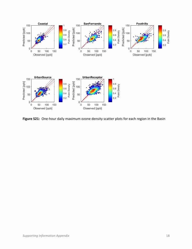
Figure S21: One-hour daily maximum ozone density scatter plots for each region in the Basin


Figure S22: Eight-hour daily maximum ozone density scatter plots for each region in the Basin

for 2012


Figure S23: PM2.5 model performance regions. Black markers indicate the location of PM2.5

monitoring stations.


Figure S24: Comparison between predicted and observed daily-averaged PM2.5 concentrations


Figure S25: Time series of daily averaged PM2.5 predicted and observed concentrations in Anaheim


Figure S26: Time series of daily averaged PM2.5 predicted and observed concentrations in Central Los Angeles


Figure S27: Time series of daily averaged PM2.5 predicted and observed concentrations in Mira Loma, the monitoring site with the highest PM2.5 concentrations in the Basin


Figure S28: Time series of daily averaged PM2.5 predicted and observed concentrations in Riverside


Figure S29: Difference in temperature (Title24 – Baseline) for each hour of the day at three locations across the Basin. Grey hashed cells indicate that differences are not statistically significant (p>0.05).


Figure S30: Difference in planetary boundary layer height (Title24 – Baseline) for each hour of the day at three locations across the Basin. Grey hashed cells indicate that differences are not statistically significant (p>0.05).


Figure S31: Difference in annual averaged 9am to 3 pm 10 m wind speed (Title24 – Baseline) for each hour of the day at three locations across the Basin. Grey hashed cells indicate that differences are not statistically significant (p>0.05). Seasonal profiles in Redlands are highlighted in red because seasonal differences in wind speed are not statistically significant (p>0.05) at that location.


Figure S32: Difference in annual maximum ventilation coefficient (Title24 – Baseline) for each hour of the day at three locations across the Basin. Grey hashed cells indicate that differences are not statistically significant (p>0.05).


Figure S33: A) Change in ozone season average daily maximum 8-hour and 1-hour ozone concentrations at Redlands (Title24-Baseline) as the fractional change in UVR is varied from 0 (no change) to 1 (maximum change). B) Corresponding change in ozone design values.


Figure S34: A) Average change in winter PM2.5 concentrations. B) Average change in spring

PM2.5 concentrations. C) Average change in summer PM2.5 concentrations. D) Average change in

autumn PM2.5 concentrations. Grey hashed cells indicate areas where changes are not

statistically significant (p>0.05). Image represents 3x3 cell moving average. Changes are largest

in the winter and autumn months.


Figure S35: A) Change in the number of 8-hour O3 federal standard (75 ppb) exceedance days (Scenario IV – Scenario I) with the assumption that UVR does not change with widespread installation of cool roofs. The green circle indicates the location of the highest 8-hour O3 measured DVs in the Basin. B) Change in the number of 8-hour O3 exceedance days with the assumption that UVR increases are consistent with the maximum possible increase based on roofing products currently available (Scenario V – Scenario I). Grey hashed cells indicate that differences in 8-hour daily maximum O3 concentrations are not statistically significant. (p > 0.05) Image represents 3x3 cell moving average.


Figure S36: Fraction of each grid cell that is paved

Documents

Air-quality implications of widespread adoption of cool