NONCOMBATANT EVACUATION OPERATIONS IN USEUCOM

GRADUATE RESEARCH PAPER

Mark A. Scheer, Major, USAF AFIT/IOA/ENS/11-05

DEPARTMENT OF THE AIR FORCE AIR UNIVERSITY

AIR FORCE INSTITUTE OF TECHNOLOGY

Wright-Patterson Air Force Base, Ohio

APPROVED FOR PUBLIC RELEASE; DISTRIBUTION UNLIMITED

The views expressed in this thesis are those of the author and do not reflect the official policy or position of the United States Air Force, Department of Defense, or the U.S. Government.

AFIT/IOA/ENS/11-05

NONCOMBATANT EVACUATION OPERATIONS IN USEUCOM

GRADUATE RESEARCH PAPER

Presented to the Faculty

Department of Operational Sciences

Graduate School of Engineering and Management

Air Force Institute of Technology

Air University

Air Education and Training Command

In Partial Fulfillment of the Requirements for the

Degree of Master of Science in Operational Analysis

Mark A. Scheer

Major, USAF

June 2011

APPROVED FOR PUBLIC RELEASE; DISTRIBUTION UNLIMITED

AFIT/IOA/ENS/11-05

NONCOMBATANT EVACUATION OPERATIONS IN USEUCOM

Mark A. Scheer Major, USAF

Approved: __________//SIGNED//_____________ 3 Jun 11 Dr John O. Miller, Civ, USAF (Advisor) Date

iv

AFIT/IOA/ENS/11-05

Abstract

The purpose of this research was to examine Noncombatant Evacuation

Operations in the USEUCOM area of responsibility. The processes that make up a NEO

are collection of evacuees, verification of identity, security screening, and transportation

to a safe haven. Understanding the complex interactions between process building blocks

can enlighten military planners aiding them in accomplishing this critical mission faster,

safer, and more efficiently. Specifically, this graduate research project focused on

identifying areas where efficiency could be improved by modeling the evacuation process

using discrete-event simulation. The effort resulted in a general, flexible Noncombatant

Evacuation Operation Arena model. The model was designed to be adapted to specific

operational plans and run using varying assumptions to validate the plan.

Recommendations to implement the model in validating current plans and for further

research are discussed.

v

Table of Contents Page

Abstract .............................................................................................................................. iv

Table of Contents .................................................................................................................v

List of Figures .................................................................................................................... vi

List of Tables ................................................................................................................... viii

I. Introduction .....................................................................................................................1

Background...................................................................................................................1 Problem Statement........................................................................................................2 Objectives .....................................................................................................................3 Scope ............................................................................................................................4 Real World Perspective on NEO ..................................................................................5 Methodology.................................................................................................................8 Assumptions and Limitations .....................................................................................10 Model Construction ....................................................................................................12

II. Methodology .................................................................................................................15

Overview ....................................................................................................................15 Baseline Conceptual Model ........................................................................................17 Embellishments to the Conceptual Model ..................................................................22 Measures of Performance ...........................................................................................25 Arena Model ...............................................................................................................26 Model Embellishments within Arena .........................................................................39 Verification and Validation ........................................................................................43

III. Results and Analysis ...................................................................................................45

Overview ....................................................................................................................45 Completion Time Analysis .........................................................................................47 Additional Measures and Critical Factors ..................................................................53 Summary.....................................................................................................................58

IV. Recommendations.......................................................................................................59

Significance of Research ............................................................................................59 Recommendations for Action .....................................................................................59 Recommendations for Future Research......................................................................61 Summary.....................................................................................................................62

Appendix: Blue Dart ..........................................................................................................63

Bibliography ......................................................................................................................66

Vita ....................................................................................................................................67

vi

List of Figures Page

Figure 1. NEO Baseline Conceptual Model .................................................................... 18

Figure 2. Embellishment 1 Model ................................................................................... 23

Figure 3. Embellishment 2 Model .................................................................................... 24

Figure 4. Embellishment 3 Model ................................................................................... 25

Figure 5. Baseline Arena Model ...................................................................................... 27

Figure 6. Mad Rush Arrival Schedule ............................................................................. 28

Figure 7. Wait and See Arrival Schedule ......................................................................... 29

Figure 8. Orderly Arrival Schedule ................................................................................. 29

Figure 9. Mad Rush Arrivals from Arena ........................................................................ 30

Figure 10. Wait and See Arrivals from Arena ................................................................. 30

Figure 11. Orderly Arrivals from Arena .......................................................................... 31

Figure 12. Define Evacuees Submodel ............................................................................ 32

Figure 13. SPOE Arena Model: Ferry Fills to Capacity .................................................. 34

Figure 14. TSH Arena Model Buses Fill to Capacity ...................................................... 38

Figure 15. Ferry Schedule SMART Submodel ................................................................ 40

Figure 16. Scheduled Ferry Transportation Arena Logic ................................................ 41

Figure 17. Scheduled Aircraft TSH Submodel ................................................................ 42

Figure 18. Two ECC Model Logic .................................................................................. 43

Figure 19. Paired-t Test for BASE Completion Times .................................................... 49

Figure 20. Paired-t Test EMB2 Completion Times ......................................................... 50

Figure 21. Paired-t Test EMB3 Completion Times .......................................................... 52

vii

Figure 22. BASE vs EMB1 Average Wait Times ........................................................... 55

Figure 23. EMB1 vs EMB2 Performance Paired-t Test: 4 hour Departure Schedule ..... 57

Figure 24. EMB1 vs EMB2 Performance Paired-t Test: 2 hour Departure Schedule ..... 57

viii

List of Tables Page

Table 1. Ferry Transportation Variables and Attributes .................................................. 37

Table 2. NEO Factor Modeling Assumptions.................................................................. 44

Table 3. Transportation Capacity Across the Scenarios .................................................. 46

Table 4. Completion Times.............................................................................................. 48

Table 5. Average ECC Completion Times ...................................................................... 52

Table 6. BASE vs EMB1 System Performance ............................................................... 54

Table 7. EMB1 vs EMB2 Performance ............................................................................ 56

1

NONCOMBATANT EVACUATION OPERATIONS IN USEUCOM

I. Introduction

Background

The United States government goes to great lengths to protect American citizens

(AMCITS) including those who live and work abroad. The Department of State (DOS),

through the many embassies around the globe, manages the task of looking after our

citizens overseas. Recent world events rife with political turmoil and regional instability

show the necessity for continued vigilance. When a particular country becomes unstable,

one option that is available to the Ambassador in that country is to order an evacuation of

the U.S. citizens. When an Ambassador deems an evacuation necessary, the embassy

can call on the Department of Defense (DoD) to provide assistance in the form of a Non-

Combatant Evacuation Operation (NEO).

DoD’s regional joint command, United States European Command (USEUCOM),

is responsible for planning and executing NEOs for the countries in its Area of

Responsibility (AOR). These operations are infrequent, however when an Ambassador

directs the evacuation of a country it must be done quickly and efficiently. Regulatory

guidance for NEO exists within Joint Publication 3-68: Noncombatant Evacuation

Operations. However, it does not describe the nuts and bolts of how to execute a NEO

efficiently.(JCS, 2010) A NEO is a complex operation that can range from permissive to

hostile type environments and are largely subject to the unique physical characteristics of

2

the environment and the interactions between the US, host nation, and various other non-

state actors.

No two NEOs will look the same. Factors such as the physical topography of a

country, availability of transportation resources, threat situation, and many more make

each one a unique experience. However because NEO is fundamentally about

transporting people from one location to another, they are all constructed of the same

process building blocks regardless of other differences. The processes that make up a

NEO are collection of evacuees, verification of identity, security screening, and

transportation to a safe haven. Understanding the complex interactions between process

building blocks can enlighten military planners aiding them in accomplishing this critical

mission faster, safer, and more efficiently. This project’s goal is to gain a better

understanding of NEO using discrete-event simulation. Specifically, creating a discrete-

event simulation model of the process and then varying the structure and input factors to

highlight efficiencies and critical factors that drive performance of the system.

Problem Statement

In 2009, EUCOM/J3 approached AFIT seeking efficiencies in the general NEO

process and hoping to craft operations into repeatable, visibly positive events throughout

the command’s area of responsibility.(Gregg, 2010) To that end Major Aimee Gregg

conducted research and created a discrete-event simulation NEO model in Arena. This

project is a continuation of that effort to replicate a NEO in order to describe and

understand the process. Specifically, find the areas causing, or most likely to cause

delays or complications in the process.(Gregg, 2010) Based on that effort, this project

3

further develops and validates the NEO model. With our updated model and a more

robust series of experiments, this project seeks to further define the process delays.

Despite recent real-world NEOs conducted in the last six months that USEUCOM

participated from a planning perspective, accurate data is still extremely limited. This

limitation underscores the supreme importance of sensitivity analysis in the project.

Finally, Major Chris Olsen is conducting a simultaneous and related study

focusing specifically on the Evacuation Control Center (ECC) within the NEO process.

Also using discrete-event simulation, the ECC model and results will be incorporated into

this modeling effort with the goal of producing a higher fidelity, more complete model.

Objectives

The primary objective of our study is to better understand the processes of a NEO

and their interactions, with the goal of reducing the time required to complete a NEO.

Since sufficient data is not available to model the setup process, our study of the

operation begins when the first evacuee arrives at the ECC and ends when the last

evacuee disembarks at the safe haven. Since no two NEOs are the same, the intent is to

explore different structural options and highlight favorable and unfavorable trade-offs

between resources committed and completion time improvements.

The secondary objective is to identify the most critical variables. By comparing

different modes of transportation or NEO process structures, the benefits of those

different modes of transportation or NEO structures can be determined. This information

will aid the planners in allocating their limited resources most efficiently to realize the

biggest gains or minimize losses.

4

As with any model, the assumptions made in the development process have an

enormous effect on the outcome of a study. While the numerical answers may only apply

in a narrowly defined situation, the model output should identify critical areas and

general trade-offs that will guide the planning of future NEOs or specific areas for future

research.

Scope

DOS is the lead federal agency in the conduct of NEOs and DoD assistance may

or may not be required or practical. Therefore NEO from USEUCOM’s perspective

focuses on those occasions where DOS requires significant security and heavy lift in

uncertain or hostile environments. Once DoD support is authorized by the Secretary of

Defense (SECDEF), USEUCOM NEO planners will try to ascertain the nature of the

environment, hostile or permissive, to determine what posture the assisting force will

need to assume. In the majority of cases the Marine Expeditionary Unit (MEU) is DoD’s

most readily equipped and available force to operate in the varying environments.

Because the inherent uncertainties of combat may overshadow any useful information

that can be gained about the system, it is assumed that the modeled NEO is occurring in a

semi-permissive environment. In this environment there is general political violence

occurring in the country significant enough to warrant an evacuation. However, that

violence is not being directed at Americans or American interests. Additionally, the host

government is allowing the evacuation and possibly even providing assistance.

Unlike the Lebanon NEO operation in 2006, DOS will not pay for the evacuees’

transportation back to the United States. The number of people desiring evacuation was

5

unexpectedly large because of citizens who evacuated not because of the threat, but

because of the free trip. While the Joint Publication states that the United States is the

preferred safe haven, it recognizes that in some cases that is not practical. DOS primarily

focuses on getting the evacuees immediately out of harm’s way and safely to a temporary

safe-haven (TSH). From there, the expectation has been that evacuees secure follow-on

transportation through their own means. As the end of a common evacuation process, the

TSH is a logical end for the NEO model.

Real World Perspective on NEO

As recent world events have shown in Libya and Egypt, Noncombatant

Evacuation Operations are not a distant possibility. They are a very real and present

challenge that faces U.S. embassies on a daily basis.(Standifer, 2008) In fact it would

probably surprise most Americans how frequently our activities overseas are significantly

disrupted. In the past twenty years the Department of State has handled more than 270

evacuations successfully.(GAO, 2007) These evacuations occur for any number of

different reasons and come in just about any shape and size. In the wake of the 2006

Lebanon Evacuation, the Government Office of Accountability published report GAO

08-23, “Evacuation Planning and Preparations for Overseas Posts Can Be Improved.”

The document begins by putting a framework around the different kinds of evacuation

operations:

State evacuates staff, dependents, or private American citizens in response to various crises, including civil strife, terrorist incidents, natural disasters, conventional war threats, and disease outbreaks. For example, according to information compiled by State,

of the 89 evacuations over the past 5 years, almost

half were clustered in the Middle East, Turkey, and Pakistan. Twenty-three of

6

these evacuations were due to the impending U.S. invasion of Iraq in early 2003; the remaining evacuations in the Middle East, Turkey, and Pakistan were due primarily to terrorist threats or attacks. Ten other evacuations in Southeast Asia resulted from the outbreak of severe acute respiratory syndrome (SARS) in the spring of 2003, and nine in the Caribbean were due to hurricanes. During 2006 and 2007, State evacuated 11 posts for various reasons, including civil unrest, elections that could lead to civil unrest, a coup attempt, a U.S. embassy bombing, a hurricane, and war.(GAO, 2007)

Not only do these operations run the gamut in reason and scale, each one is just as

different in how they are conducted. Each country has different physical characteristics,

different ports, different layouts, different transportation resources. The United States

has a different presence in each country and a different relationship with each of the Host

Nations. Additionally, the population of Americans living and traveling in countries

varies widely. The Department of State faces significant challenges conducting this type

of emergency operation in such a wide range of locations. Fortunately, they have a wide

range of available resources up to and including the U.S. Military.

Although State cannot order American citizens to leave a country due to a crisis, State officials said they provide varying degrees of assistance to Americans wishing to leave. State officials told us American citizens typically leave on commercially available flights; the U.S. government does not generally arrange transportation for departing American citizens. State sometimes assists by creating greater availability of commercial transport, such as by requesting U.S. flag carriers to schedule more flights. Infrequently, when commercial transportation is not available, State officials contract transportation for American citizens.

More serious crises may require the assistance of DOD; according to

data compiled by State, DOD has provided assistance on only four occasions in the past 5 years. For example, during a period of civil unrest in a Caribbean country in 2004, DOD provided military assistance to help embassy personnel and their families depart the country. On very rare occasions, large numbers of American citizens depart the country on U.S. government-contracted and U.S. military transportation.(GAO, 2007)

7

When DOS is required to call upon the DOD for assistance with a NEO it is significant

event. One of the chief issues is coordination between the two departments. In the past,

unique roadblocks have come up which restricted coordination and inhibited operations.

When State requires assistance with a large-scale evacuation (e.g., during the 2006 evacuation from Lebanon), it may request help from DOD. Guidance for coordination between State and DOD is included in an MOA [Memorandum of Agreement]

meant to define the roles and responsibilities of each agency in

implementing such large-scale evacuations. According to the MOA, State is responsible for the protection and evacuation of all U.S. citizens abroad and is generally responsible for evacuating U.S. citizens. However, State may request assistance from DOD to support an evacuation. Once DOD assistance has been requested, DOD is responsible for conducting military operations to support the evacuation in consultation with the U.S. ambassador. During an evacuation, the MOA calls for coordination between State and DOD through a liaison group responsible for evacuation planning and implementation.(GAO, 2007)

This GAO report had the same genesis as most of the literature available on NEO, after

action review of operations with the intention of gathering lessons learned for future

operations. While most of the literature focused on things like the interaction between

departments and different recommendations to the planning process, there was a

particularly interesting recommendation on how to incorporate a computer simulation

such as Arena into the planning process.

Rehearsals can be executed in simulation. A realistic constructive simulation could be modeled to replicate a NEO. This would greatly assist planners in visualizing their course of action, determining the capacity of key nodes and the expected duration and through-put in these key nodes. Many problems and misunderstandings can be avoided by conducting rehearsals.(Davis, 2007)

The idea of identifying problems and limitations in the NEO process is precisely what

this research is about. While this particular effort looks at more generic cases, a well-

built, flexible model could be easily adapted to incorporate all the assumptions for a

8

specific plan. Then running the scenario against a number of different arrival

distributions would highlight the weak links in the plan. This sort of analysis could be

particularly beneficial especially when you understand that most gains in efficiency of a

NEO rely on matching capacity throughout the system.

The art in execution here is always being able to match lift capability to demand and processing time at each node. Rehearsals, accurate F-77 data, timely and accurate reporting, and current intelligence all contribute to being able to anticipate demand for lift. Exceeding the holding capacity of AAs and ECCs in country results in increased risk to designated Evacuees.(Davis, 2007)

This research aims to lay the groundwork for this type of planning analysis. The general

NEO structure does not lend itself well to in-depth study because it is constantly being

varied. Additionally, too many assumptions have to be made in order to build the model

flexible enough to be applied to different situations. Starting with a general model and

applying all the constraints of a specific scenario could lead to worthwhile gains for

planners working on a specific operation.

This study focuses on the general NEO model. To fill in many of the small

assumptions initially, the evacuation of Lebanon served as a template. As it was the site

of an evacuation in 2006 and continues to be an area of interest in the world, it makes a

solid case study for this effort. Meetings, emails, and phone calls with the NEO planners

at USEUCOM, the geographic command responsible for a Lebanon NEO, guided the

model development process and aided in model validation.

Methodology

Modeling a system using discrete-event simulation requires identifying the entity

moving through the system. In this case it is logical that evacuees are the entities moving

9

in the system. In simulation, the entities move independent of one another, which is only

partially accurate in this case. When families travel they tend to behave as a unit rather

than independent entities. Therefore the entities in this model are family units instead of

individual evacuees. These family unit entities more closely resemble the way evacuees

actually move through the system vice individual travelers.

Joint Publication 3-68 outlines the framework of the NEO process. That process

begins with a Warden System message that notifies the AMCITS of a DOS

recommendation to evacuate the country and instructs them to proceed to the nearest

Evacuation Control Center (ECC) for transportation out of the country. At the ECC,

evacuees are screened, processed (registered in the NEO tracking system), and prepared

for embarkation aboard some form of transportation. Ideally the ECC is collocated with

the port of embarkation (POE) allowing evacuees to directly board a ship or aircraft for

transport to the TSH. This process is the simplest version of NEO and describes the

baseline NEO model.

The true power of discrete-event simulation is in comparing different versions of

a system to find statistical differences in system performance. Additionally, NEO is a

system that varies every time it is implemented providing very little historical data upon

which to base modeling assumptions and form a hypothesis. Therefore, the model

architecture must be as flexible as possible allowing the researcher to test many different

scenarios and variables. By changing the scenario and comparing statistics to a baseline

model, the researcher can demonstrate the effect of a change on the system. In this case,

the baseline model is modified to represent different scenarios and compare the effect of

10

those changes on system performance. Embellishments begin with variations in the

number/scheduling of available transports. Further scenarios look at geographically

separating the ECC and the POE, additional ECCs to increase capacity, and varying

availability of different modes of transportation on these advanced scenarios.

In order to compare the various scenarios, meaningful measurements of system

performance must be defined and collected from the model variations. For a NEO the

most obvious measure of performance is overall time to complete the evacuation.

Average and maximum evacuees time waiting for transportation, transportation queue

lengths, and transportation utilization provide a more in-depth understanding of system

differences. Ideally, that understanding will eventually lead to a set of NEO planner

guidelines for future operations.

Assumptions and Limitations

Understanding the assumptions that go into a model is the key to drawing out

useful insight into the process. Some key assumptions made about the NEO system

include threat environment, set-up time, evacuee arrivals, and transportation availability.

As described in the problem scope above, the threat environment is semi-

permissive. The uncertainties in a combat environment can obscure system

characteristics. Combined with that, the objective of this study is the system itself and

not the interactions with the combat environment.

It takes time to put forces in place to execute any operation and NEO is no

exception. The MEU, the force of choice to execute NEO, is in short supply. Obviously

there are significant impacts to a NEO based on the availability and travel time to get the

11

MEU into country to begin the evacuation. The vast number of possible scenarios to get

the ECC set up makes modeling this function impractical, and therefore it is assumed for

our model that when the first evacuee shows up, the entire system is ready to handle its

max capacity. Interactions between setup and process time are not studied.

Evacuee arrivals are a function of several different factors ranging from threat

scenario and perceived benefit to other paths to safety for an evacuee. Unfortunately, the

arrival distribution cannot be assumed away ergo three possible scenarios are examined: a

mad rush case, a wait and see case, and an orderly departure flow. The mad rush case

assumes that most evacuees feel immediately threatened and a majority show up soon

after the Warden System message is released and tapers off as the number of AMCITS

in-country dwindles. Conversely, the wait and see case assumes that most people are

willing to wait it out to see if the situation will improve. When State determines that the

evacuation is drawing to a close and announces that the last transports are leaving,

evacuees rush to the ECC to get out before the window closes. This results in a late peak

in arrivals. The last case is the planner’s ideal, a constant average arrival rate of evacuees

into the ECC. While it is difficult to conceive of scenarios where this would actually

occur, most simple planning calculations are based on this assumption making it a good

basis for comparison.

Transportation availability and scheduling can greatly affect the waiting times and

overall completion times of a NEO. In order to examine some possible transportation

scenarios immediate availability and contract flexibility are assumed. An extension of

the set-up time assumption, the transporters (boats, airplanes, etc) are ready to depart as

12

soon as passengers are ready for them. Furthermore, those transporters work around the

clock supporting any schedule required of them. This assumption allows the comparison

of several different transportation employment scenarios.

Model Construction

Discrete-event simulation is a powerful analysis technique for gaining a true

understanding of how a system operates. A few of the more applicable advantages of

simulation include obtaining insight on the interaction of variables and the importance of

variables to the performance of the system.(Banks, 2010) NEO planners must understand

how the different factors they control influence the performance of the entire system.

Simulation also allows for bottleneck analysis to discover where things are being delayed

excessively.(Banks, 2010) Obviously this is right in-line with researching the NEO

process. Finding the places where bottlenecks are likely to occur and reallocating

resources to the right places can make the difference in a successful operation. The

correct application to the NEO system has the potential for significant gains in process

understanding that could ultimately result in faster, safer evacuation operation.

Arena, a software package from Rockwell Automation Inc., is the discrete-event

simulation software used to build the NEO model. Arena was chosen because it

combines the ease of use found in high-level simulators with the flexibility of simulation

languages.(Kelton, 2010) A few advanced features of Arena that directly benefit a NEO

model include submodels and transporters.

Submodels are blocks that can be used within a model to group various pieces of

model logic. These blocks have basic connection variability, a title, and little else.

13

However, the submodel opens a new screen where standard blocks can be used to code a

particular task. This structure is incredibly useful for studying a NEO because it allows

for quick changes in structure. By building all the different tasks required in a NEO such

as the ECC, ferry transportation, etc within different submodels, they can be combined in

varying configurations, tested and quickly rearranged to another variant.

Another particularly handy feature of Arena is the transporter. A transporter is a

device that will move an entity around the simulation mimicking a truck, boat, etc. This

logic aids the modeler translate conceptual transportation functions into simulation logic.

Free-path transporters move freely through the system without encountering delays. The

time to travel from one point to another depends only on the transporter velocity and

distance to be traveled.(Kelton, 2010) Transporters have two disadvantages when it

comes to modeling a NEO. First, they are typically either active or inactive and cannot

be controlled using Arena’s resource schedule logic. Fortunately, the software comes

with some helpful, pre-built submodels called SMARTs. One of these SMARTs is a

schedule program for transporters. Using this SMART the schedule drawback is easily

overcome. Second, transporters have a capacity of one. Therefore to transport more than

one entity at once, those entities must be batched together. Even with these manageable

limitations, the transporter is a very effective tool when looking at a transportation

problem like a NEO.

Arena is the perfect tool for a study of this scope. It is powerful software with all

the functionality and flexibility to effectively model this process. Additionally, its user

14

interface is simple enough to allow beginning users to model a complicated system in a

reasonable amount. This is critical is making a study of this nature viable.

15

II. Methodology

Overview

Analyzing a Noncombatant Evacuation Operation is a difficult problem. Not only

are no two operations the same, there are almost too many factors to account for. Even

with a seemingly endless number of configurations and factors, certain efficiencies can

still be gained by studying a select number of key interactions in a simplified version of

the system. By building a discrete-event simulation model of the system in Arena, those

key factors can be isolated in a simplified system and mathematically compared

highlighting how those factors drive system performance.

The strength of simulation is that ability to compare the performance of a baseline

system against a modified system to determine the impact of the modifications. In our

study, the baseline model is the simplest version of a NEO. Starting with a baseline

model of the simplest configuration it is easy to modify or add pieces one at a time to get

the isolated effect of a specific change.

The baseline model of the system represents the minimum action required to

evacuate a country. To aid in making reasonable assumptions, the evacuation of Lebanon

was chosen as the scenario for this model. Lebanon was chosen because it is within

EUCOM’s area of responsibility, the US executed a NEO there in 2006, and it remains an

area of interest because of the ongoing political unrest. The process consists of evacuees

arriving at the ECC, required processing to safely transport the people, and transporting

them to a safe haven. For this scenario the safe haven is the country of Cyprus. While it

may seem like a simplistic representation, it provides a solid basis for comparison

16

because it minimizes the need for detailed assumptions that a more complicated model

must make.

Even with this simplified model we must make some assumptions. The biggest of

these is the arrival of evacuees to the ECC. After reading Major Gregg’s research and

discussing NEO specifics with Major Olsen and Mr Mike Livingston at EUCOM, it was

decided to look at the arrival of about 5,000 people spread over two days. The

assumption is that this estimate represents a high number of evacuees. Mr. Livingston

estimates that 50 people per hour as the realistic processing capacity of a standard MEU

ECC team. Under ideal conditions he estimates that rates of 100 people are possible.

Therefore the arrival of just over 100 people per hour should stress the system while not

overwhelming it.

The actual arrival times of those 5,000 people are described in the three scenarios

modeled: a mad rush case, a wait and see case, and an orderly departure flow. The mad

rush case assumes that most evacuees feel immediately threatened and a majority show

up soon after the Warden System message is released and tapers off as the number of

AMCITS in-country dwindles. Conversely, the wait and see case assumes that most

people are willing to wait it out to see if the situation will improve. When State

determines that the evacuation is drawing to a close and announces that the last transports

are leaving, evacuees rush to the ECC to get out of the country before the window closes.

This scenario results in a late peak in arrivals. The last case is the planner’s ideal, a

constant average number of evacuees arriving every hour at the ECC. While it is difficult

17

to conceive of scenarios where this would actually occur, most simple planning

calculations are based on this assumption making it a good basis for comparison.

In all scenarios the arrivals are limited to 48 hours. Cutting off the arrivals

completely at a set time allows for a better comparison of system completion times. Over

the two days of arrivals our model has to react to surges and lulls in arrival activity. By

cutting off the arrivals with the system still under load, the models demonstrate their

ability to quickly clear out a backlog of people. In the end, these assumed scenarios

should test the performance of the NEO model under a realistic range of arrival

conditions.

From the baseline model under these arrival conditions our study looks at the

effect of three different factors: scheduling boats versus filling them to capacity;

evacuating people on boats versus using aircraft; and using an additional ECC to process

people, with the additional requirement of transporting them from the second ECC to the

port. Scenarios incorporating these factors are designed to demonstrate to EUCOM the

trade-offs between: two different methods of contracting transportation; use of boats or

aircraft when given the choice; and potential advantages of adding a geographically

separated ECC.

Baseline Conceptual Model

Modeling the baseline NEO using discrete-event simulation requires defining the

entity moving through the system. In this case evacuees are the entities moving in the

system, more precisely, family units of evacuees. In simulation, the entities move

18

independent of one another. However, when families travel they tend to behave as a unit

rather than independent entities. These family unit entities more closely resemble the

way evacuees actually move through the system vice homogeneous individual entities.

The process these family units follow is basically a straight line starting with their arrival

at the ECC and ending with their arrival at the safe haven airport shown in Figure 1.

Evacuees Arrive at ECC;Entities are defined

as an evacuee population

Evacuees loaded directlyonto three ferries that run

as soon as they are full

ECC processes EvacueesEstimate a median

processing rate of 50 people per hour.

Evacuees arrive at Safe Haven

Evacuees transportedfrom port to airport onsix buses running assoon as they are full

Evacuees are briefed oncurrent situation and travel options from

Safe Haven

Evacuees released tocontinue or stay as

desired

Figure 1. NEO Baseline Conceptual Model

How the evacuees arrive to the ECC is an important piece that will drive system

performance throughout the simulation. The arrival rate will be dictated by the current

political situation and perceived threat in the country. The three different arrival

scenarios used for our study are the mad rush, the wait and see, and the orderly departure.

The system starts empty and idle and the arrival distribution varies with the scenario.

Additionally, the evacuees do not balk in the model. This assumption is reasonable since

the study focus is system performance after the people get in the door of the ECC.

Additionally, what happens outside the ECC is aggregated into the arrival distribution. In

the absence of Warden system performance data, the arrival rate is a big assumption.

Analytic comparisons of the three different scenarios shores up this factor.

19

Since the model looks at family units an assumption must be made about the

population make-up. The family group attribute models the fact that the entities that are

actually moving through the system are family units and not individuals. For example,

children are not going to be put on a separate bus from their parents. While precise data is

not available to define this factor for a given country, US census data provides a

reasonable approximation. Therefore each family unit size is defined based on the typical

size of the US family limited to five family members maximum. Single people comprise

30% of the family units, 32% are couples, 17% are units of three, 14% are fours, and the

last 7% are units of five. Families larger than five in the census data were rolled into the

five person units. The benefit gained from modeling larger families does not justify the

effort involved to add them into the model. This attribute defines the number of people

in the family so the entity will occupy the correct number of seats on a transportation

mode. However, by randomly generating the number of people assigned to each family

unit it is difficult to control the exact number of people in the simulation. Therefore, the

number of family entities is held constant at 2,100 to allow for comparison of the

different scenarios. That number of family units generates between 4,500 to 5,000

people.

The next part of the modeled arrival process defines other characteristics of each

evacuee family unit. This research does not use any additional characteristics past family

size, however this capability was built into the model for two reasons. First, the research

on the ECC being done by Major Olsen does require the use of different family

20

characteristics. By building this functionality into this model structure, Major Olsen’s

ECC can easily be plugged into this model giving a higher level of fidelity. Second,

having the ability to define characteristics built into the basic model structure provides

flexibility to model different scenarios in future research. An example of this could be

research looking at the effects of a rank structure or priority evacuees such as designated

very important persons on the overall flow.

The first checkpoint for the evacuees, the ECC, is the most labor intensive of the

NEO processes. However, this study essentially treats that process as a “black box”. The

details of that process are subject of a simultaneous study conducted by Major Chris

Olsen and focused solely on the ECC process. His ECC submodel is designed to plug

directly into this model of the overall process. While the ECC can be modeled by a

simple delay, Major Olsen’s baseline model is used for all the data runs. As a check on

the ECC logic, Mike Livingston at USEUCOM, the resident MEU/ECC expert, provided

an estimate of ECC processing rates. He estimates that a single MEU ECC team can

realistically process about 50 evacuees per hour. Major Olsen’s baseline ECC performs

close to the estimate and provides more detail to the model.

Once the evacuees are processed through the ECC they proceed directly to the

Sea Port of Embarkation (SPOE). At the SPOE the evacuees walk straight to the

boarding area and wait for a ferry to arrive and a sufficient number of people to fill it.

This simulation assumes that all three ferries are the same size and filled to capacity of

350 passengers before departing. The vessel San Gwann, a high-speed catamaran type

21

passenger-car ferry owned by Virtu Ferries Ltd, is representative of the type used in

previous evacuations. The San Gwann has a capacity of 429 passengers and a speed of

39 knots. Prior to departing, the ferries are delayed briefly for an estimated loading time.

In the baseline scenario ferries sail when they are loaded to capacity and therefore run on

a variable schedule. They sail at a constant average speed of 39 knots over the distance

of 138 nautical miles from the SPOE to the safe haven. The distance, 138 NM, is the

distance from the port of Beirut to the Port of Larnaca on the island of Cyprus. No

additional delays (e.g. rough seas) are modeled. The passengers disembark at the safe

haven port incurring a short delay for unloading time.

At the safe haven the evacuees are briefed en mass on the current situation and the

travel options at this point. Upon completion of that briefing, the passengers are

transported via six buses to an airport at the safe haven. This step is required because the

airport offers the most options for continued travel from this location. The six buses run

continuously, departing only when filled to capacity until the ferry in port is empty. The

buses have a capacity of 65 passenger per bus, about the size of a medium school bus and

travel at an average speed of 35 miles per hour from the SPOE to the airport. The

Larnaca Airport is eight miles from the Larnaca Seaport. No additional delays such as

traffic jams are modeled.

Upon reaching the safe haven airport the evacuees are free to make their own

follow-on arrangements and the formal evacuation process is complete. This is where the

baseline model ends, as this is where State and DoD end their responsibility for the

22

evacuees. At this point evacuees are free to wait out the turmoil here or proceed to any

number of other locations.

Embellishments to the Conceptual Model

The first embellishment to the baseline model simply expands control over the

function of the ferry transporters. In this case the majority of the model remains intact

with the changes impacting only one part of the process, shown in the double square in

Figure 2. In the baseline model the boats ran continuously between the safe haven and

the SPOE, departing when filled to capacity. Therefore the number of trips during a given

time period would vary depending on the demand. In some cases the ferries would stop

just long enough to fill before setting out on another trip and other times they would sit in

the port partially filled waiting on more passengers. In this embellishment, the ferries

depart on a schedule regardless of the number of passengers. This means that a given

evacuee will wait no longer that the interval between departures. However, ferries are

not completely filled when they travel, meaning more trips are required to carry the same

number of people. This embellishment demonstrates the tradeoff between waiting time

for the evacuees and efficient use of the ferries. The same type of ferries (350 passenger

capacity and 39 knot speed) is used in both cases.

23

Evacuees Arrive at ECC;Entities are defined

as an evacuee population

Evacuees loaded directlyonto three ferries that run

on a set schedule regardless of passengers

ECC processes EvacueesEstimate a median

processing rate of 50 people per hour.

Evacuees arrive at Safe Haven

Evacuees transportedfrom port to airport onsix buses running assoon as they are full

Evacuees are briefed oncurrent situation and travel options from

Safe Haven

Evacuees released tocontinue or stay as

desired

Figure 2. Embellishment 1 Model

The second embellishment, shown in Figure 3, is another variation on the

transportation block, the double square in the figure. It changes the mode of

transportation from a continuous running boat to scheduled air traffic. The aircraft

modeled is a Boeing 767 that has a capacity of 276 passengers with an estimated speed

over this distance of 400 knots. The flight to the Larnaca airport is 155 NM and unlike

the boat does not require a bus ride in Cyprus. It is important to note that while this

scenario uses aspects of the Lebanon scenario (distances and surrounding transportation),

it is purely to demonstrate modeling flexibility and show comparisons that may be

applicable in other countries. In Lebanon the Beirut International Airport is not a viable

option for the USEUCOM planners.(Livingston, 2011a) The flights are scheduled

because the logistics of this type of flight do not allow it to follow the capacity scheme.

The flights go once every four hours around the clock.

24

Evacuees Arrive at ECC;Entities are defined

as an evacuee population

Evacuees loaded directlyonto aircraft that run

on a set schedule regardless of passengers

ECC processes EvacueesEstimate a median

processing rate of 50 people per hour.

Evacuees arrive at Safe Haven

Evacuees are briefed oncurrent situation and travel options from

Safe Haven

Evacuees released tocontinue or stay as

desired

Figure 3. Embellishment 2 Model

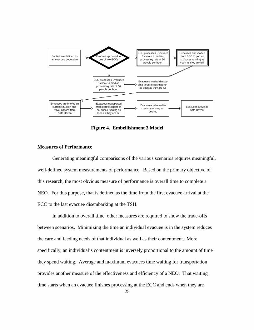
The third and final embellishment looks at the overall structure of the NEO instead of

modes of transportation. In this version, the transportation is back to ferries loaded to

capacity like the baseline model. The difference here is the addition of a second ECC

site. Figure 4 shows the system differences required to accommodate the additional

processing capacity. In this scenario there isn’t room at the port to set up a second ECC

processing team and therefore they set up at the American embassy 15 miles from the

port. This doubles the ECC processing capacity at the cost of adding a bus ride from the

second ECC to the port. The buses here are also modeled as 65 passenger vehicles with

an average speed of 35 miles per hour with no other delays.

25

Entities are defined asan evacuee population

Evacuees loaded directlyonto three ferries that run

as soon as they are full

ECC processes EvacueesEstimate a median

processing rate of 50 people per hour.

Evacuees proceed to one of two ECCs

Evacuees arrive at Safe Haven

Evacuees transportedfrom ECC to port onsix buses running assoon as they are full

Evacuees are briefed oncurrent situation and travel options from

Safe Haven

Evacuees released tocontinue or stay as

desired

ECC processes EvacueesEstimate a median

processing rate of 50 people per hour.

Evacuees transportedfrom port to airport onsix buses running assoon as they are full

Figure 4. Embellishment 3 Model

Measures of Performance

Generating meaningful comparisons of the various scenarios requires meaningful,

well-defined system measurements of performance. Based on the primary objective of

this research, the most obvious measure of performance is overall time to complete a

NEO. For this purpose, that is defined as the time from the first evacuee arrival at the

ECC to the last evacuee disembarking at the TSH.

In addition to overall time, other measures are required to show the trade-offs

between scenarios. Minimizing the time an individual evacuee is in the system reduces

the care and feeding needs of that individual as well as their contentment. More

specifically, an individual’s contentment is inversely proportional to the amount of time

they spend waiting. Average and maximum evacuees time waiting for transportation

provides another measure of the effectiveness and efficiency of a NEO. That waiting

time starts when an evacuee finishes processing at the ECC and ends when they are

26

loaded onto a transport ready to depart for the TSH. Average and maximum

transportation Queue lengths are another measure of system performance. Being

prepared for the correct number of people in the waiting area is critical to keeping the

grumbling down. Transportation utilization, measured by average number of passengers

per trip, is an easy check to ensure the ferries or aircraft are operating efficiently. Ideally,

understanding how a NEO structure performs based on the different measures will lead to

a set of NEO planner guidelines for future operations.

Arena Model

Every NEO is unique. That fact demands that a simulation model of a NEO

system is built using an extremely flexible architecture. While this research is built

around three basic comparisons, the model must be flexible enough to change as new and

more interesting questions arise. Therefore, it seems natural to take advantage of Arena’s

submodel structure. Figure 5 shows a screenshot of the baseline model in Arena.

At the highest level, the model appears as a series of four submodel processes connected

by assign and record blocks documenting process statistics. This format makes changing

NEO structures very easy since all of the process logic is grouped and contained in that

submodel. To change processes simply remove or re-order the submodel of interest and

replace or duplicate it to create a new system.

27

Figure 5. Baseline Arena Model

Evacuee family units are generated using a create node. That node simply

generates the family entities according to one of three schedules representing the different

arrival schedules. Arrival schedules in Arena allow the modeler to specify arrival rates

over time. The arrival rate is the mean number of arrivals per hour. That parameter

defines the exponential arrival distribution that generates random, Poisson-process

arrivals. The model contains three, 48-hour arrival schedules. Over that 48-hour period

the specified mean arrival rate changes every four hours.

The first schedule, Mad Rush, mimics a rush to get out of a country as soon as the

evacuation is announced. The rush of evacuees tapers off as the country empties. The

bar graph in Figure 6 shows the average hourly arrival rate as a function of time.

28

45

75

6560

55

4540

3530 30

2520

0

10

20

30

40

50

60

70

80

0-4 4-8 8-12 12-16 16-20 20-24 24-28 28-32 32-36 36-40 40-44 44-48

Time in Hours

Figure 6. Mad Rush Arrival Schedule

Wait and See, the second arrival schedule emulates a scenario where the evacuees

are unsure of what to do. Instead of proceeding directly to the ECC to evacuate they wait

for more information or a change in the situation before deciding whether or not to leave

the country. This results in a delayed rush at the ECC as shown in the Figure 7 bar graph.

The third and final arrival schedule is an orderly departure scheme. This schedule

is the planner’s ideal where there is steady average rate of arrivals at the ECC. While not

realistic in the real world, this scheme is the most common one used in planning

operations. The Orderly arrival schedule is shown in Figure 8.

29

2025

30 3035

4045

5560

65

75

45

0

10

20

30

40

50

60

70

80

0-4 4-8 8-12 12-16 16-20 20-24 24-28 28-32 32-36 36-40 40-44 44-48

Time in Hours

Figure 7. Wait and See Arrival Schedule

44 44 44 44 44 44 44 44 44 44 44 44

0

5

10

15

20

25

30

35

40

45

50

0-4 4-8 8-12 12-16 16-20 20-24 24-28 28-32 32-36 36-40 40-44 44-48Time in Hours

Figure 8. Orderly Arrival Schedule

When the entities are actually generated, the arrivals look a little different due to

the fact that the arrivals are random and the schedules represent the average number of

arrivals during a given time frame. Figure 9 shows an example of the Arena generated

30

Mad Rush arrivals for a single replication. While it is easy to recognize the general shape

of the Mad Rush schedule, the actual arrivals vary quite a bit for each replication.

41

33

4744

92

83

56

82

58

7974

80

52

68

6065 64 63

49

64

4450

3842 44

33 3431

3632

3538

29

4238

32

18

33 33

25 26 2623

27 25

12

0 00

10

20

30

40

50

60

70

80

90

100

1 2 3 4 5 6 7 8 9 10 11 12 13 14 15 16 17 18 19 20 21 22 23 24 25 26 27 28 29 30 31 32 33 34 35 36 37 38 39 40 41 42 43 44 45 46 47 48

Time in Hours

Figure 9. Mad Rush Arrivals from Arena

Figures 10 and 11 show similar examples from Arena of actual Wait and See and

Orderly arrivals. Again, he basic shape of the arrival distributions are preserved while

adding the element of random arrivals. Once generated the entities flow into a submodel,

Describe Evacuees, where attributes are assigned to the individual family units.

1916 16 17

2328

22 24

35 3734

27

43

2326 24

42

2932

39

49 51

43

5346

38

51

40

63

52

68

55

64 6662

51

70

57

47

7176

92

65

76

4841

49

10

10

20

30

40

50

60

70

80

90

100

1 2 3 4 5 6 7 8 9 10 11 12 13 14 15 16 17 18 19 20 21 22 23 24 25 26 27 28 29 30 31 32 33 34 35 36 37 38 39 40 41 42 43 44 45 46 47 48

Time in Hours

Figure 10. Wait and See Arrivals from Arena

31

41

30

50

40

47

56

4447

3841

48

38

52 51 5156

46

37

44

5147

50

40

5551

39

47 4852

3740

48

35

41

32

4146 46 46

59

47

33

49

4145 45

32

00

10

20

30

40

50

60

70

1 2 3 4 5 6 7 8 9 10 11 12 13 14 15 16 17 18 19 20 21 22 23 24 25 26 27 28 29 30 31 32 33 34 35 36 37 38 39 40 41 42 43 44 45 46 47 48

Time in Hours

Figure 11. Orderly Arrivals from Arena

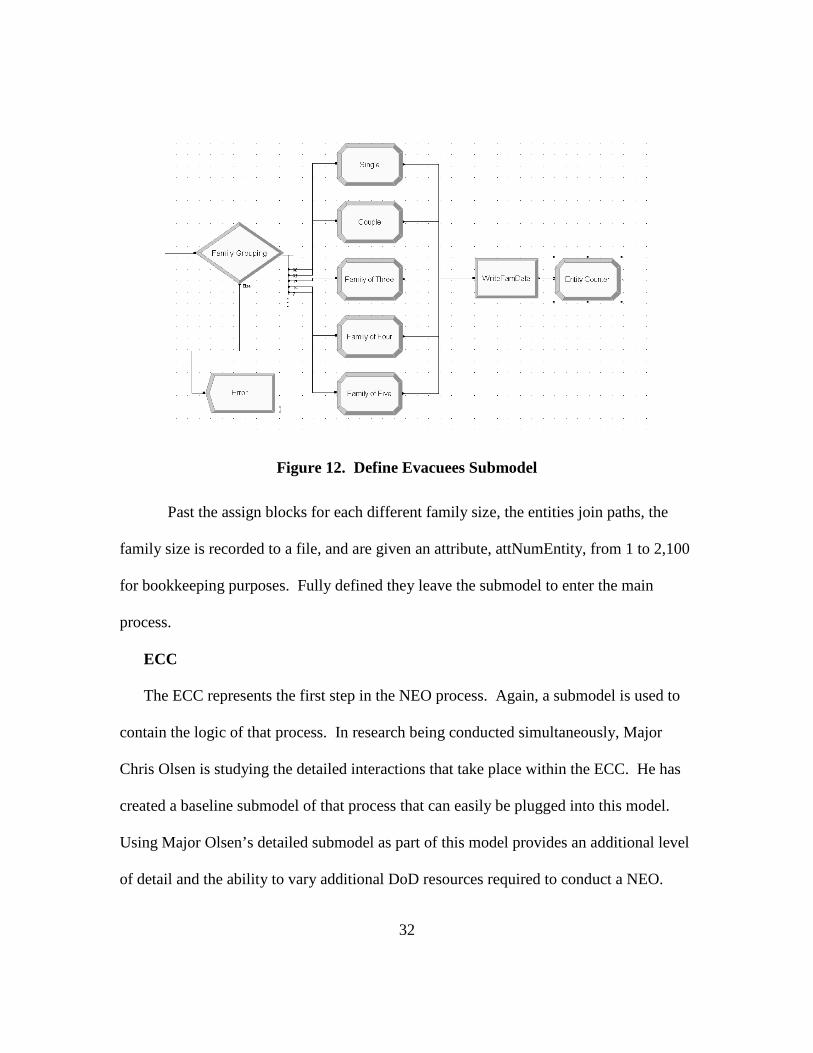
Upon entering the Describe Evacuees submodel, shown in Figure 12, the 2,100

family unit entities encounter the logic structure that assigns a number, 1,2,3,4, or 5 to the

attribute attNumFam representing the number of people in the family. The logic structure

consists of a decision node that splits the entities n-ways by chance. Thirty percent of the

entities are defined as single individuals, 32% are couples, 17% are units of three, 14%

are families of fours, and the last 7% are families of five. After the split, each branch

goes into an assign block where additional attributes can be assigned depending on the

scenarios being studied.

32

Figure 12. Define Evacuees Submodel

Past the assign blocks for each different family size, the entities join paths, the

family size is recorded to a file, and are given an attribute, attNumEntity, from 1 to 2,100

for bookkeeping purposes. Fully defined they leave the submodel to enter the main

process.

ECC

The ECC represents the first step in the NEO process. Again, a submodel is used to

contain the logic of that process. In research being conducted simultaneously, Major

Chris Olsen is studying the detailed interactions that take place within the ECC. He has

created a baseline submodel of that process that can easily be plugged into this model.

Using Major Olsen’s detailed submodel as part of this model provides an additional level

of detail and the ability to vary additional DoD resources required to conduct a NEO.

33

An alternative ECC representation used during development of this model is a single

delay block. Based on previous research and discussions with EUCOM J3 planners, a

good estimate for the ECC throughput is about 50 people per hour.(Livingston, 2011b)

With Major Olsen’s baseline ECC model installed, the ECC output is close to the

estimate. Estimated rates are based on discussions with Mike Livingston from

USEUCOM. As a former Marine responsible for training and certifying MEUs, Mike has

first hand experience with ECC training exercises. Since he was comfortable with 50

people per hour as an advertised throughput, that throughput is most likely closer to the

minimum than the maximum number. The ECC model provides a reasonable output rate,

between 60-80 people per hour, which has little impact on the scenario comparisons in

this study.

Right after leaving the ECC submodel, basic data is collected on the evacuees’

progress. A record block documents the time at which each entity departs the ECC and a

counter records the total number of evacuees processed. This data is output as a statistic

and written to a data file.

Transport Evacuees from SPOE to TSH

In an ideal situation, the evacuees proceed out of the ECC directly onto waiting

transportation, in the baseline model ferry boats. For the baseline model, it is assumed

that the Sea Port of Embarkation (SPOE) is a short walk from the ECC. This is simulated

with a short delay adding more detail to the model that can be expanded in future

scenarios. While the evacuees will have to get from the ECC to the transportation

34

somehow, beyond that there is no data or known scenario to base this delay on. In future

cases this could be an issue that warrants more detailed analysis. However, in this model

it is estimated with a random draw from a normal distribution, mean of 3 minutes and

variance of 0.5 minutes. This delay is short enough with a small variance so it does not

have much affect on the system as a whole.

Within this submodel, the bulk of the logic carries out the function of getting the

correct number of people onto the ferries at the correct times. Figure 13 is a screenshot

of that logic in Arena. This is more complicated because the entities are family units,

which is a different count than the number of individuals loaded onto a ferry. Those

counts also vary from ferry to ferry throughout the simulation. Therefore a series of new

variables and attributes were created simply to track the number of individuals on the

ferry.

Figure 13. SPOE Arena Model: Ferry Fills to Capacity

35

The first assign block includes several commands beginning the task of counting up

the number of potential passengers on a ferry. Initially a variable, FerryFull sums the

attNumFam attributes and assigns the current sum to each entity as the attribute

attFerryFull. This is a sum of the total number of individuals represented by the entities

currently waiting for transportation. In the same block another variable, FerryCount, is

summing the number of entities. To prevent potential issues later in the batch block, all

entities are assigned an attribute, attFerryCount, with a nominal value of 1,000. Last,

each entity receives an attribute, attStartFerryWT, which marks the time their wait for

transportation began.

A two-way decide node limits the number of people on each ferry. If an entity’s

attFerryFull is less than the ferry capacity minus five, then it enters the batching queue

waiting for the ferry to fill. Ferry capacity is coded as a variable, FerryCap, to allow

quick changes for comparisons. Ferry capacity minus five simplifies the logic of

identifying the last entity on board. By putting a line in the sand there, the entity that is

more than that value, but less than FerryCap is identified as the last passenger, and

follows a different path to the batch queue. While this system will leave up to 4 seats

empty on the boat, it picks a final entity and ensures that the ferry is not over capacity.

The last entity enters an additional assign block that redefines attFerryCount as the

current tally of FerryCount, zeros FerryCount and FerryFull, and assigns attLastOnFerry

= 98, for that entity to preserve that designation for later. When the last entity enters the

36

batch queue it defines the batch size as attFerryCount, all the waiting entities are grouped

as one boatload, and they all proceed onto the boat.

Since transporters move between defined locations within the simulation, they may or

may not be where they are needed when an entity needs transportation. Therefore, when

the new boatload entity leaves the batch node it enters a node where it requests a ferry.

When the ferry arrives, the entity delays for a loading time defined as a normally

distributed time with a mean of three minutes and variance of one minute. The loading

time for the ferry is assumed to be quick because there are no assigned seats and multiple

passengers can walk down a gangplank and get settled onboard simultaneously.

Additionally, since loading time is proportionally small compared with total enroute time,

it does not factor much into the overall transportation time. After the loading delay, the

model logic calculates and records attFerryWait, the time spent waiting for a ferry, for

each entity.

The ferry then departs the SPOE for the TSH seaport. The trip time is based on the

ferry speed of 39 knots over a distance of 138 NM, the distance from Beirut to Larnaca.

The appropriate distances are defined in Arena in the Ferry.Distance module. Upon

arrival at Larnaca, the boatload encounters a normally distributed unloading delay with a

mean of three minutes and variance of one minute.

37

Table 1. Ferry Transportation Variables and Attributes

In this scenario it is assumed that the ferry has been contracted for the duration of the

evacuation and therefore would precede directly back to Beirut to wait for the next

boatload whether they are waiting or not. Therefore, the model logic immediately starts

the empty ferry on the 138 NM journey back to Beirut and releases it for the next entity.

Conceptually, the evacuees are standing on the dock in Larnaca as the entity exits this

submodel. The total time between the back door of the ECC and the dock in Larnaca is

recorded prior to entering the next submodel.

The Temporary Safe Haven

For the evacuees at the TSH, the formal evacuation process is almost over. Off of

boat at the port they receive a short, approximately 20 minute updated situation briefing

on what happens now. The arrival briefing at the TSH is modeled with a normally

distributed delay with a mean of 18 minutes and variance of 4 minutes. Since it is a mass

Variable Name Definition FerryFull The number of individuals to be loaded on the next ferry (sum of

entities’ attNumFam) FerryCount The number of family units (entities) that make up FerryFull FerryCap Capacity of the ferry in use Attribute Name Definition

attFerryFull Assigns current sum of individuals on a ferry to each entity attFerryCount Assigns current sum of family units to each entity attLastOnFerry Designates the last family unit loaded on each ferry attStartFerryWT Records the time each entity began the wait for the ferry ride attFerryWait Records the time each entity spent waiting for the ferry ride

38

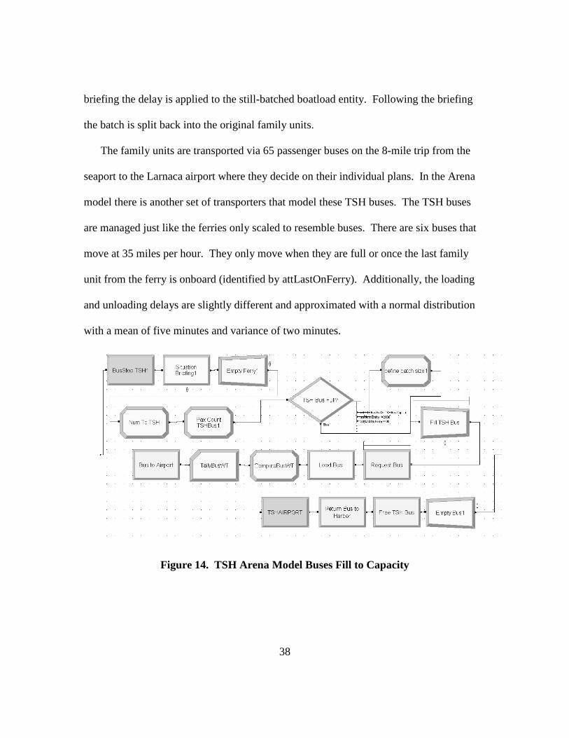
briefing the delay is applied to the still-batched boatload entity. Following the briefing

the batch is split back into the original family units.

The family units are transported via 65 passenger buses on the 8-mile trip from the

seaport to the Larnaca airport where they decide on their individual plans. In the Arena

model there is another set of transporters that model these TSH buses. The TSH buses

are managed just like the ferries only scaled to resemble buses. There are six buses that

move at 35 miles per hour. They only move when they are full or once the last family

unit from the ferry is onboard (identified by attLastOnFerry). Additionally, the loading

and unloading delays are slightly different and approximated with a normal distribution

with a mean of five minutes and variance of two minutes.

Figure 14. TSH Arena Model Buses Fill to Capacity

39

Once the evacuees arrive at the airport they exit the submodel. Outside the submodel

arrival time at the TSH airport is recorded and the entities exit the simulation. This

completes the baseline NEO model.

Model Embellishments within Arena

The first embellishment to the baseline model adapts the ferries from continuously

running shuttles to scheduled trips. The majority of the model remains intact with the

addition of logic submodel to schedule the ferries and some changes within the ferry

transportation submodel allowing the ferries to run less than full.

The additional submodel, containing transporter-scheduling logic, was adapted

directly from SMART151 that came with the Arena software. Converting that submodel

was a simple matter of renaming the blocks, changing the transporter references from the

example, and adapting the expression to make the ferries run on the desired schedule.

SMART151 was designed as a capacity schedule. In this application it was adapted to

turn a specific ferry on at a specific time to provide more control over the ferries. The

updated submodel is shown in Figure 15. The two blocks highlighted in the upper black

square were changed to keep the correct schedule index and run delay in the event of an

entity getting out of sync in the system. Another entity on a constant hourly arrival

schedule (not pictured) was created to release the hold at the correct time. Once the

transporters were running on the correct schedule, the difficult part is batching the

evacuees. To aid in the batching logic contained in the ferry transportation submodel, the

two additional blocks highlighted in the lower black square in Figure 15 were added.

40

Immediately before a ferry is scheduled, an assign block records the number of entities

currently in the “Waiting For Ferry” queue in a one-dimensional array,

FerryQueueCount, indexed on a variable, BoatNum. BoatNum is a variable that counts

the number of ferries trips. Next, a signal block empties the “Waiting For Ferry” queue

allowing them to continue to the batch node. Together these two blocks are the key to

sequencing the evacuees.

Figure 15. Ferry Schedule SMART Submodel

To accommodate the ferry schedule embellishment, some significant changes had

to be made in the logic that batches evacuees for the ferry ride. The ferry transportation

Arena logic is shown in Figure 16. The logic starts out the same counting the number of

individuals and assigning the count, FerryFull, to the entity as an attribute, attFerryFull.

At the decide node however things are different. If attFerryFull is less than the ferry

41

capacity, FerryCap, the entity is sent to the Wait For Ferry queue. If attFerryFull is

greater than FerryCap, the entity is sent into Overflow to wait for another ferry. When

the ferry is set to arrive, the entities in the Wait For Ferry queue are released. The entities

are counted in an assign block and that number is compared to the previously recorded

FerryQueueCount for the current BoatNum. That determines the last entity on the ferry

and allows the batch to be completed. Once that happens the counters are reset and the

Overflow is released to re-enter the logic from the beginning. Statistics are collected in

the same manner as in the baseline model. The remainder of the first embellishment

model is identical to the baseline isolating the impact of scheduled versus continuous

ferry transportation.

Figure 16. Scheduled Ferry Transportation Arena Logic

The second embellishment, another variation on the transportation block, changes

the mode of transportation ferries to scheduled aircraft. All the components of this

embellishment have essentially been described already. Most of the model is the same as

in the first embellishment with the number of transporters, schedule, capacity,

42

loading/unloading times, and speed changed to mimic aircraft instead of high-speed

ferries. Additionally, the distance from Beirut to Larnaca airport, 155 NM, is slightly

further than the distance between seaports. Until the TSH, the logic structure remains the

same since it is assumed that the ECC is located at the airport in embellishment two

versus the seaport in the baseline model.

The logic change at the TSH is shown in Figure 17. Since there is no longer a

requirement to bus the evacuees anywhere once they arrive at the TSH, there is no need

for the bus logic from the ferry models. In the aircraft case there is only a briefing,

splitting the aircraft batch and counting the arrivals at the TSH. The rest of the model is

identical to the baseline model.

Figure 17. Scheduled Aircraft TSH Submodel

The third and final embellishment, Figure 18, also uses components previously

described only connected together in yet another configuration. This version adds a

second ECC that is not located at the port, but instead at the American Embassy 15 miles

away. Adding a second ECC is as simple as copying and pasting the ECC submodel. A

decide node splits the evacuees 50-50 between the two ECCs. For ECC 1 everything is

identical to the basline model from this point forward. For ECC 2, an additional

43

submodel, Gnd Trans to Port, is added. The logic structure in this submodel is identical

to the logic used to simulate the TSH buses in the baseline model and later in this model.

That routine was simply adapted to allow two different types of buses in the same model.

Figure 18. Two ECC Model Logic

At the SPOE all the evacuees are combined back into a single path to complete the

evacuation. This embellishment best illustrates the flexibility of submodels in Arena and

how easy it can be to test different scenarios.

Verification and Validation

One of the key steps in the model building process is verification and validation of

the model. Verification is the process of checking the model to ensure that it was coded

correctly. This is the process of checking to make sure it runs all the way through and the

entities proceed through the model as expected. For the baseline NEO model and all the

embellishments this was mainly conducted using Arena’s built in animation and readouts

of different variables along the way. The model behaved as intended, matching the

conceptual model.

44

Validation is a much more difficult task. Validation is checking the conceptual and

constructive models against reality to ensure that they are accurately modeling the system

of interest. In case of NEOs this is very difficult because little data exists from previous

operations. In the absence of data many assumptions had to be made. Those NEO

system factor assumptions are summarized in Table 2. If that data existed, the model

could be configured to match the given scenario and the output matched against real-

world data to confirm that it is behaving correctly. In the absence of data, the model

must be validated by expert opinion. In this case, model output is checked by subject

matter-experts to confirm the model is behaving correctly.

Table 2. NEO Factor Modeling Assumptions

Factor Baseline Emb 1 Emb 2 Emb 3Ferry Speed 39 knots 39 knots -- 39 knotsFerry Capacity 350 Pax 350 Pax -- 350 PaxFerry Loading Time NORM (3,1, 46) NORM (3,1, 46) -- NORM (3,1, 46)Ferry Distance 138 NM 138 NM -- 138 NMNumber of Ferries 1 to 4 1 to 4 SCHED 0 1 to 4Walk to Terminal NORM(3,0.5, 50) NORM(3,0.5, 50) NORM(3,0.5, 50) NORM(3,0.5, 50)Aircraft Speed -- -- 400 TAS --Aircraft Capacity -- -- 276 Pax --Aircraft Loading Time -- -- NORM(25,5,47) --Flight Distance -- -- 155 NM --Number of Aircraft -- -- SCHEDULE --TSH Bus Speed 25 mph 25 mph -- 25 mphSPOE Bus Speed -- -- -- 35 mphBus Capacity 65 Pax 65 Pax -- 65 PaxBus Loading time NORM(5,2,48) NORM(5,2,48) -- NORM(5,2,48)TSH Bus Distance 8 8 -- 8SPOE Bus Distance -- -- -- 15Number of TSH Buses 6 6 -- 6Number of SPOE Buses -- -- -- 6Briefing Delay NORM(18,4,42) NORM(18,4,42) NORM(18,4,42) NORM(18,4,42)

45

III. Results and Analysis

Overview

The presentation of the results mostly consists of raw comparisons between the

different scenarios. By looking at these general comparisons, breakpoints and other areas

of interest stand out. Once the comparisons of interest are selected a paired-T test is used

to show the statistical differences. Since several different measures of performance were

taken, the scenarios are compared on a couple of different scales where applicable. It is

important to understand that while output from this simulation may be a reasonable

estimate of actual system performance, this is not the objective. The strength of

simulation is showing the statistically (and/or practically) significant differences in the

performance of two varied systems, not predicting a specific outcome.

The baseline model (BASE) uses one ECC located at the port of embarkation,

ferries that run continuously, and a bus at the TSH that delivers the passengers to the

TSH airport. Embellishment 1 (EMB1) changes the ferry departures from continuous to

scheduled every 8, 6, 4 or 2 hours. Embellishment 2 (EMB2) replaces the ferries with

scheduled aircraft changing the capacity, speed, and eliminating the bus ride at the TSH.

Finally, Embellishment 3 (EMB3) uses the BASE transporter, but adds a second,

geographically separated ECC that doubles the capacity at the cost of another bus trip.

This study varied parameters in three distinct areas: the four scenarios; the three

evacuee arrival distributions; and four different levels of available primary transport.

Comparing results while varying three variables simultaneously makes interpretation

difficult. Therefore, we begin by calculating a reasonable level of transportation starting

46

with the estimated ECC output of 50 evacuees per hour, the capacity of the ferry or

aircraft, and the roundtrip time to the TSH and back. Table 3 shows the baseline level of

transportation for the different models, baseline and embellishments.

Table 3. Transportation Capacity Across the Scenarios

A comparison of the scenarios and arrival distributions is made using the

calculated base level of transportation. Once the preferred scenarios are identified, we

vary the level of transportation to show system sensitivity to the amount of transportation

available.

Statistical differences of the measures of performance between different scenarios

are shown using the Paired-t Test at a 95% confidence level. Since we are interested

finding the differences in these four systems, a technique referred to as common random

numbers was used. Common random numbers synchronizes the random numbers

generated across the different model variations. Therefore, all four scenarios are exposed

to the same load on any given replication. This provides a more accurate comparison

because differences are due to the system and not to a difference in the stress placed on

the system. Using common random numbers means that the scenarios are no longer

statistically independent from each other. The Paired-t Test is the appropriate test to use

Transportation Capacity

(evacuees/trip)ECC Capacity

(evacuees/hour)

Max Time between departures

(hours/per trip)Number of Transports

Required

Resulting per hour Transport Capacity

(evacuees/hour)

BASE 350 50 7 2 boats (about 1 every 4 hrs) 87

EMB 1 350 50 7 1 boat every 4 hours 87

EMB 2 276 50 4.5 1 airplane every 4 hours 69

EMB 3 350 100 2.5 3 boats (about 1 every 3 hrs) 131

47

when the scenarios are not statistically independent. The tests were conducted with

Arena’s Output Analyzer software using results exported from the model. Each scenario

and variation was run for 20 replications.

Completion Time Analysis

The primary objective of our study is to reduce the time required to complete a

NEO. Therefore the primary measure of performance is the overall NEO completion

time, the time in hours from the first evacuees arriving at the ECC to the last evacuee

arriving at the TSH.

While completion time includes the entire system as defined above, the ECC,

which is not varied in the baseline scenario does not affect the difference overall

completion times. The model outputs ECC completion time as one measure of

performance. A quick comparison between the different runs confirms that the ECC

completion time only varies with the arrival distribution. This holds true for

embellishments 1 and 2 as well since the ECC is the same throughout those models.

Table 4 shows the completion times for each of the different scenarios run at each of the

arrival distributions. A couple of things stand out immediately.

48

Table 4. Completion Times

Time in Hours 95% HW Time in Hours 95% HWMad Rush 73.23 0.30807 73.089 0.03239

Orderly 73.074 0.36169 73.086 0.02746Wait and See 77.012 0.54475 77.085 0.03742

Time in Hours 95% HW Time in Hours 95% HWMad Rush 79.89 0.84425 55.986 1.2074

Orderly 80.305 0.93929 56.081 0.82376Wait and See 81.475 0.90579 56.274 0.61871

BASE (2 Continuous Ferries) EMB1 (Ferry every 4 hours)

EMB2 (Aircraft every 4 hours) EMB3 (3 Continuous Ferries)

While completion times vary widely across the different scenarios, the variations

due to the arrival distributions follow a distinct pattern. Typically the Mad Rush

completion times are close to the Orderly completion times while the Wait and See

completion times are significantly longer. Figure 19 shows the statistical comparisons

between the three completion times for the BASE model. The top test shows that Mad

Rush completion time is not statistically different that the Orderly completion time. The

next two tests demonstrate that the Wait and See completion times are statistically

different than the Orderly and Mad Rush times respectively.

49

Figure 19. Paired-t Test for BASE Completion Times

This result is similar for EMB1 and EMB3 as for the BASE model. This tells us

that our system can cope with an early rush fairly well. There is enough capacity within

the system to absorb an initial rush of people and recover to finish in nearly the same

time as it would with a steady average arrival rate.

In reality, a difference of about four hours might not make much difference. This

tells us that under these conditions our systems are robust enough to handle the three

arrival distributions. The planner can then feel more comfortable knowing that as long as

the actual arrival distribution falls somewhere in between these his system can handle it.

The EMB2 scenario, shown in Figure 20, is a little different. The top two tests

here show that Mad Rush and Wait and See are both statistically the same as Orderly,

while the third test shows that Mad Rush and Wait and See are statistically different. In

Mad Rush vs Orderly

Wait and See vs Orderly

Wait and See vs Mad Rush

50

the second test, Wait and See compared with Orderly, zero barely clips the edge of the

confidence interval.

Figure 20. Paired-t Test EMB2 Completion Times

The EMB2 system is still behaving in a similar fashion as the other three in

regards to the different arrival distributions. The slight difference here is a function of

the speed of the transporter. Since the aircraft enroute time is significantly shorter than

the ferry enroute time, the differences in the system are slightly smaller. In this case that

is enough to get zero into the confidence interval and make those two completion times

appear the same.

These results hint that our resources are correctly sized for the arrival scenarios

used. It can absorb the early surge so there aren’t too few resources. Likewise, it does

Wait and See vs Orderly

Wait and See vs Mad Rush

Mad Rush vs Orderly

51

drag a little under a late surge suggesting that there aren’t excessive idle resources.

Again, the difference in average completion times is pretty small, about 5 hours, which in

most scenarios is below the planner’s threshold of interest. This does not mean that the

system changes are not a factor; it means that all the systems compared are well suited to

handle the given arrivals. However, knowing this kind of information for a specific

scenario, a planner could adjust the planning factor to that scenario to better approximate

the number of resources required to meet the demand. Note that this planning factor

would be specific to each operation plan as differences in the scenario assumptions can

drive changes in that planning factor as demonstrated in the next set of comparisons.

Armed with a basic understanding of how the different arrival distributions affect

a given model, the remaining comparisons between models use the Orderly arrival

distribution. This reduces the variable factors to highlight differences between systems.

Looking at the completion times, what stands out the most are the results from

EMB3. The completion times are significantly lower and statistically significant as

shown in Figure 21. The cause is obvious, increased ECC capacity. Table 5 shows the

same pattern in the comparison of the average ECC completion times.

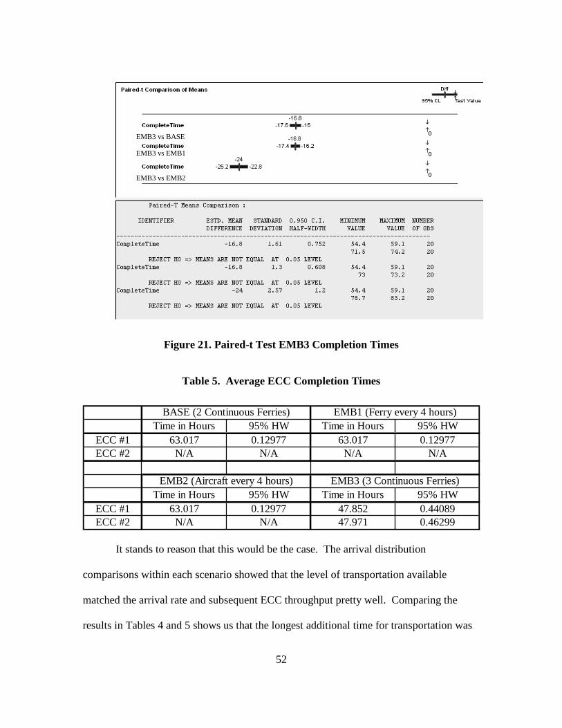
52

Figure 21. Paired-t Test EMB3 Completion Times

Table 5. Average ECC Completion Times

Time in Hours 95% HW Time in Hours 95% HWECC #1 63.017 0.12977 63.017 0.12977ECC #2 N/A N/A N/A N/A

Time in Hours 95% HW Time in Hours 95% HWECC #1 63.017 0.12977 47.852 0.44089ECC #2 N/A N/A 47.971 0.46299

BASE (2 Continuous Ferries) EMB1 (Ferry every 4 hours)

EMB2 (Aircraft every 4 hours) EMB3 (3 Continuous Ferries)

It stands to reason that this would be the case. The arrival distribution

comparisons within each scenario showed that the level of transportation available

matched the arrival rate and subsequent ECC throughput pretty well. Comparing the

results in Tables 4 and 5 shows us that the longest additional time for transportation was

EMB3 vs BASE

EMB3 vs EMB1

EMB3 vs EMB2

53

less than 17 hours while the shortest was just under 9 hours. Considering that the enroute

time is about 4.5 hours, that only leaves about 4.5 hours of room for improvement.

Likewise, from the example arrival distribution in Figure 11, we expect the last evacuee

to arrive sometime in the 47th hour. That means the improvement in ECC capacity

gained from BASE to EMB3, from hour 63 to hour 47, is most likely the maximum

improvement possible.

The completion time analysis for these scenarios tell us that the systems are

balanced and able to handle the arrival rates that are set against them. If these scenarios

had been based on exact specifics from an actual operation plan, we could validate that

plan demonstrating the trade-offs in completion times between the different scenarios.

An informed decision between the scenarios can be made or risks mitigated where

options don’t exist. If the planner was still concerned about variations in the arrival

schedule, the selected system design could be tested against increasingly extreme arrivals

until the breaking point is found. Knowing how sensitive the system is to breaking lets

the planner know if they have a reasonable factor of safety built in.

Additional Measures and Critical Factors

Completion time is not the only important performance measure in NEO. Further

comparison of the four scenarios highlights a few other important measures. By

comparing the continuous ferries in the BASE scenario to the schedule in EMB1, we can

get a feel for how average waiting times and queue lengths respond to additional

transportation capacity. Again, the Orderly arrival schedule is used for the purpose of

comparison. The ferry enroute time from Beirut to Larnaca is about 4 hours. That means

54

the baseline comparison: two ferries operating continuously should be analogous to

operating on schedule of one departure every for hours. Table 6 shows the effect of an

incremental increase in transportation capacity for BASE and EMB1. They are compared

on completion time, average time waiting for the ferry, average queue length, and the

average number of passengers per trip.

Table 6. BASE vs EMB1 System Performance

2 Continuous or Departure Every 4

hrs

3 Continuous or Departure Every 3

hrs

4 Continuous or Departure Every 2

hrs

Completion Time 73.074 71.527 71.527

Average Wait Time 2.2208 2.1915 2.1915

Average Queue Length 175.01 175 175

Average # Passengers 331.99 331.99 331.99

Completion Time 73.086 72.09 72.252

Average Wait Time 2.075 1.5567 1.0495

Average Queue Length 161.12 122.62 84.168

Average # Passengers 291.06 224.91 151.82

BA

SEE

MB

1

As the number of ferries increases in the BASE scenario, the measures of

performance stay constant. Any gains from adding another boat are taken up by the boat

waiting in the port for a full load. Completion time for the EMB1 scenario stays the same

as the ferry schedule varies, however, the rest of the performance factors steadily

decrease as shown in Figure 22. That figure shows a series of average wait time Paired-t

Tests between BASE and EMB1. The available ferries increase from top to bottom in the

figure. As the frequency of ferries increase, the average wait time, statistically different

throughout, continues to drop.

55

Figure 22. BASE vs EMB1 Average Wait Times

When compared with the BASE wait times we see EMB1 looking better and

better. This improvement comes at the cost of transportation effieciency. Table 6 also

shows how the average number of passengers per trip drop off for EMB1. By simulating

a given scenario, specifically a given arrival rate, and varying the number of transporters

available, it is easy to find the preferred balance between efficiency (number of

transports) and evacuee waiting time. Evacuee waiting time isn’t just a matter of

convience. That is time that the DOS or DoD must care for those people. At a minimum

that means food, shelter, and water and at worst in a hostile environment it means

providing protection against an attacking forces. Good planning can minimize these

risks.

The final comparison shows the effects of switching a smaller, faster vehicle.

Since the aircraft modeled in EMBs is on a schedule, it will be compared with EMB1

2 Cont. vs Sched every 4 hrs

3 Cont. vs Sched every 3 hrs

4 Cont. vs Sched every 2 hrs

56

instead of the BASE scenario. Table 7 compares EMB1 against EMB2 on two different

schedules: a departure every four hours and a departure every two hours.

Table 7. EMB1 vs EMB2 Performance

Departure Every 4 hrs

Departure Every 2 hrs

Completion Time 73.086 72.252

Maximum Wait Time 4.0957 2.0716

Maximum Queue Length 352.15 189.2

Average # Passengers 291.06 151.82

Completion Time 80.305 65.865

Maximum Wait Time 17.647 7.3345

Maximum Queue Length 1216.6 582.15

Average # Passengers 255.78 224.91

EM

B2

EM

B1

The difference in completion times stands out. On the four-hour schedule EMB1

is significantly better. On the two hour schedule this is reversed and EMB2 is

significantly better. Where the ferry is already operating with plenty of excess capacity

under the first schedule, the aircraft is still struggling to meet demand. This can be seen

in the significantly longer maximum wait time and queue lengths. Figure 23 shows the

aircraft’s statistically significant performance increase obtained when switching to the

more frequent schedule. The maximum queue length is cut in half and wait times drop

by nearly 60%. With this increase in capacity, we finally see the impact of the faster

vehicle on NEO completion times. This schedule step represents a break-point in

performance for the use of aircraft.

57

Figure 23. EMB1 vs EMB2 Performance Paired-t Test: 4 hour Departure Schedule

Despite this significant jump in performance for the aircraft, the ferry still out

performs it in maximum wait times and maximum queue lengths. Figure 24 shows that

this schedule step still represents a statistically significant increase in performance for the

ferries.

Figure 24. EMB1 vs EMB2 Performance Paired-t Test: 2 hour Departure Schedule

58

Both vehicles represent viable options operating under both schedules. While

there are significant performance differences, those differences would have to be weighed

against whatever planning restrictions were present in the particular NEO. That said the

differences in performance represent significant differences that will impact the outcome

of the operation and must be accounted for in planning and execution.

Summary

By modeling a particular NEO scenario as precisely as possible and then varying

different factors such as evacuee arrival schedules, number of ECCs, type of transport

vehicle, and transportation schedule; important changes in system performance come to

light. Most of the actual time differences in the scenarios studied are pretty small, all

system capacities are matched to the expected arrivals. This demonstrates the level of

differences that can be picked up with these comparisons. When comparing two real

world alternative plans, the differences may be much greater, but less obvious due to

differences in NEO system design.

Understanding how a NEO system reacts to changes in planning factors can help

planners to design better systems that are going to perform well under a wide variety of

conditions. It also helps those executing the plan to make better decisions to adapt the

plan to the actual conditions of the NEO.

59

IV. Recommendations

Significance of Research

The overall goal of this research is to help USEUCOM find ways to improve its

NEO planning and execution. The planning process they use is good but there is room

for improvement by using the in depth analysis techniques and dedicated research time

that an AFIT graduate student can offer. The real challenge of NEO planning and

execution is the inherent variability. It is a system that changes every time that it is

employed and involves human behavior. Studying the general NEO structure provided a

better sense of the interactions present leading to a flexible model that can be adapted to

analyze and validate a specific NEO operation plan. The scenario assumptions used in

this research do highlight some trade-offs within a general NEO system, however the real

payoff is the creation of a model structure to analyze specific scenarios.

Recommendations for Action

The ultimate desire for this project was to uncover some insights that could be

directly applied to improve the planning process. At the general level of this study there

are few direct applications. The research here does show the interactions within the

system that cause the benefits in some of the planning trade-offs. None of those trade-

offs are unexpected and that is not the true benefit of this study.

This study does show what kinds of trade-offs within the system can best be

studied using simulation. Actually seeing the relative effects on completion time, queue

length, waiting times, and transportation utilization of different system variations is the

real power of simulation. This research provides the NEO planner with a tool for

60

examining specific plans and a blueprint for what they can expect to find in a NEO

simulation.

With the tool developed, the next step in this process is to apply the tool to some

real-world NEO plans. After the planners have done the planning, site visits, and

legwork to get the details of the NEO plan in place they should meet with a NEO analyst

who can take the specific details: location(s) of the ECC(s); capacity and speed of the

buses, planes, or ferries that will actually be used; distance between the port and the

temporary safe haven; loading/unloading times based on the actual conditions at the

ports; and other such details to input into this model. Additionally, specific planning

constraints should be examined such as the physical limits of the facilities, i.e. how many

people fit into the ECC facility. Once the analyst has that specific information, the model

can easily be adapted to represent that scenario.

The next step is possibly the most critical in actually getting good information out

of the model. The NEO planner and the analyst need to discuss the planners specific

concerns about the given scenario. This may include a decision between structure

options, a plan A and plan B. That is the true power of this model. Given two potential

scenarios and accurate parameters such as number of ships, distances, etc; good

comparisons can be made giving planners real insight into how their plan might unfold.

This type of simulation will show where the system slows down and what the critical

points are. In a country that is particularly dangerous, the planner may feel the potential

exists for an extreme rush on US facilities. Understanding those concerns allows the

analyst to put a plan together that varies the correct parameters getting the planner

answers to the questions that really need to be answered.

61

In addition to being flexible, this NEO model has the advantage of short run

times. Twenty replications of a particular case can be run in a matter of seconds. That

means the analyst can run a variety of cases quickly to determine for instance what level

of a resource is particularly sensitive or which arrival pattern is particularly critical.

Flexibility and short run times also mean that applying the model to a specific plan is a

viable option. Specific models are going to be the source of the best information.

Recommendations for Future Research

There are a couple of potential avenues for future research that fit more in line

with DOS responsibilities. Since the DoD typically only gets involved in NEO in crisis

situations where DOS cannot handle the operation itself, this type of simulation and

planning is better suited to some of the bigger NEOs in permissive environments. The

nature of crisis planning can mean that the best plan developed in advance gets thrown

out quickly due to unforeseen execution constraints. The application of simulation lends

itself to a more stable process. Stable NEO situations are more in line with DOS

responsibilities and not the DoD.

Future research may lend itself more to the type of operations that DOS handles

on its own and do not require DoD resources. One of the biggest unknowns and also

biggest drivers of a NEO system is the arrival rate of evacuees at the ECC. One of the

most beneficial NEO research efforts would be to better understand the evacuee arrival

process. This has multiple parts. It begins with a better understanding of the American

population within the country of interest. Past reports on evacuation operations have

cited the F-77 report, an embassy’s list of Americans within the country, as extremely

62

lacking.(GAO, 2007) Research into methods to track Americans living or visiting a

specific country could be very beneficial to the DOS.

Another possible avenue for research takes arrivals one-step further. Once the

embassy knows how many AMCITs it needs to evacuate, it needs to contact them and

direct them to the nearest ECC so processing can begin. The Warden System currently

used has also been identified as a weak link.(GAO, 2007) A research effort into how to

better communicate with AMCITs in the event of a crisis or how to better control the rate

of arrivals to the ECC could provide better insight into NEO planning.

Summary

Discrete-event simulation is a powerful tool that can be used to find and exploit

trade-offs between different system configurations. The application of simulation to

NEO planning highlights some of the trade-offs planners can make to tailor system

performance. The crisis-action nature of most NEOs that DoD is involved with limits

some of the potential benefits of simulation research.

63

Appendix: Blue Dart

Politics by Other Means: The Military’s Role in International Relations

Mark Scheer, Major, USAF

mark.scheer@afit.edu

Word Count: 650

“War is a mere continuation of policy by other means.” is Carl von Clausewitz’s

most famous saying about war. It has been used time and again by soldier-scholars to

illustrate the military’s role in national policy. While the quote is as true today as when

first uttered, it has become completely inadequate in describing the military’s current role

in national policy. Military operations other than war comprise most of the Department

of Defense’s (DoD) expanding requirements. Troops have deployed around the globe

supporting secondary missions ranging from natural disaster relief to humanitarian aid

and nation building. Many of these tasks have much closer ties to the Department of

State (State) than to the DoD blurring the lines of responsibility and demanding a review

of organizational structure and functions.

The DoD mission is simple. According to defense.gov, “The mission of the

Department of Defense is to provide the military forces needed to deter war and to

protect the security of our country.” While loose interpretation allows for expansion of

the DoD mission to whatever the country needs, State’s mission speaks more directly to

many of the military operations other than war. State.gov presents the mission as:

“Advance freedom for the benefit of the American people and the international

community by helping to build and sustain a more democratic, secure, and prosperous

64

world composed of well-governed states that respond to the needs of their people, reduce

widespread poverty, and act responsibly within the international system.”

Without getting into political reasons for the changing roles, it is easy to see that

the DoD has the resources to better execute worldwide operations. With over three

million people between active duty, civilian, National Guard and Reserve and a 2010

budget of roughly $665 billion, the DoD is the largest department according to

whitehouse.gov. In comparison, State is comprised of thirty thousand people with a 2010

budget of about $50 billion is just not equipped to carry out the large scale actions its

mission statement demand. This structure often places both departments at a

disadvantage. The DoD gets tasked with humanitarian missions it is not designed or

trained to execute because it possesses the manpower. Whereas State possesses the

expertise and local knowledge to better perform the same missions, but lacks the raw

manpower to get it done. This leads to blended operations where State is the lead on

policy and makes decisions but DoD is responsible for executing. The Non-Combatant

Evacuation of a foreign country is one such instance. The Government Office of

Accountability cited some of these issues in its report on the 2006 evacuation of

Lebanon. “State and DoD’s different institutional cultures and systems impeded their

ability to work together; among other things, these differences resulted in

miscommunications and possible delays in chartering ships and planes to evacuate

American citizens.” The memorandum of agreement in place between the two

departments did not contain enough specific information on how the interactions were to

take place. While the end result was deemed successful, this evacuation highlights the

65

need for more coordination between State and DoD to effectively carry out the nation’s

international policy.

Moving forward from here requires significant effort on both sides. Regardless of

political leanings, the simple reality is both departments hold key pieces to the puzzle and

will not be effective on their own. State needs to understand what the DoD capabilities

are and what the process is to request and employ those capabilities. Likewise the DoD

needs to understand State’s mission and train its troop accordingly to execute those

missions when called upon.

For better or worse the Department of Defense holds the United States’ capability

to project not only power but also varying degrees of non-violent influence. Therefore,

the department must not limit itself to Clausewitz’s “war” as a means of executing policy

and become adept at working with the Department of State to execute the range of

international policy.

Major Mark Scheer is a graduate student in the IDE Operations Analysis program at

AFIT

Keywords: Noncombatant Evacutation, Department of State, Department of Defense,

International Policy

66

Bibliography

Banks, Jerry. Discrete-Event System Simulation. 5th ed. UpperSaddle River: Prentice Hall, 2010.

Davis, Mark A. Joint Considerations for Planning and Conducting Noncombatant

Evacuation Operations. Naval War College, Newport, RI. 2007. Gregg, Major Aimee N. Optimizing Crisis Action Planning in the Noncombatant

Evacuation Operation. Graduate Research Project, AFIT/IOA/ENS/xx-xx. School of Operations Research, Air Force Institute of Technology (AU), Wright-Patterson AFB OH, June 2010.

Government Accountability Office. State Department: Evacuation Planning and

Preparations for Overseas Posts. Washington: GPO, 2007. Joint Chiefs of Staff. Noncombatant Evacuation Operations. JP 3-68. Washington: GPO,

2010. Kelton, W. David, Randall P. Sadowski, and Nancy B. Swets. Simulation with Arena. 5th

ed. Boston: McGraw-Hill Higher Education, 2010. Livingston, Michael. USEUCOM J3 PLANNER, Stuttgart GE. Electronic mail. 10 May

2011a. Livingston, Michael. USEUCOM J3 PLANNER, Stuttgart GE. Telephone interview. 25

April 2011. Standifer, Kate M. Working Together during Noncombatant Evacuation Operations.

Naval War College, Newport, RI. 2008.

REPORT DOCUMENTATION PAGE Form Approved OMB No. 074-0188

The public reporting burden for this collection of information is estimated to average 1 hour per response, including the time for reviewing instructions, searching existing data sources, gathering and maintaining the data needed, and completing and reviewing the collection of information. Send comments regarding this burden estimate or any other aspect of the collection of information, including suggestions for reducing this burden to Department of Defense, Washington Headquarters Services, Directorate for Information Operations and Reports (0704-0188), 1215 Jefferson Davis Highway, Suite 1204, Arlington, VA 22202-4302. Respondents should be aware that notwithstanding any other provision of law, no person shall be subject to an penalty for failing to comply with a collection of information if it does not display a currently valid OMB control number. PLEASE DO NOT RETURN YOUR FORM TO THE ABOVE ADDRESS. 1. REPORT DATE (DD-MM-YYYY)

16-06-2011 2. REPORT TYPE

Graduate Research Paper 3. DATES COVERED (From – To)

Dec 2010 - Jun 2011 4. TITLE AND SUBTITLE Noncombatant Evacuation Operations in USEUCOM

5a. CONTRACT NUMBER

5b. GRANT NUMBER

5c. PROGRAM ELEMENT NUMBER

6. AUTHOR(S) Scheer, Mark, A., Major, USAF

5d. PROJECT NUMBER 5e. TASK NUMBER

5f. WORK UNIT NUMBER

7. PERFORMING ORGANIZATION NAMES(S) AND ADDRESS(S) Air Force Institute of Technology Graduate School of Engineering and Management (AFIT/EN) 2950 Hobson Street, Building 642 WPAFB OH 45433-7765

8. PERFORMING ORGANIZATION REPORT NUMBER AFIT/IOA/ENS/11-05

9. SPONSORING/MONITORING AGENCY NAME(S) AND ADDRESS(ES) USEUCOM/J3 Attn: Jeff White, LT, USN CMR 480 Box 3075 DSN: (314) 430-4286 APO, AE 09128 e-mail: whitejk@eucom.mil

10. SPONSOR/MONITOR’S ACRONYM(S) 11. SPONSOR/MONITOR’S REPORT NUMBER(S)

12. DISTRIBUTION/AVAILABILITY STATEMENT APPROVED FOR PUBLIC RELEASE; DISTRIBUTION UNLIMITED. 13. SUPPLEMENTARY NOTES 14. ABSTRACT

The purpose of this research was to examine Noncombatant Evacuation Operations in the USEUCOM area of responsibility. The processes that make up a NEO are collection of evacuees, verification of identity, security screening, and transportation to a safe haven. Understanding the complex interactions between process building blocks can enlighten military planners aiding them in accomplishing this critical mission faster, safer, and more efficiently. Specifically, this graduate research project focused on identifying areas where efficiency could be improved by modeling the evacuation process using discrete-event simulation. The effort resulted in a general, flexible Noncombatant Evacuation Operation Arena model. The model was designed to be adapted to specific operational plans and run using varying assumptions to validate the plan. Recommendations to implement the model in validating current plans and for further research are discussed. 15. SUBJECT TERMS Noncombatant Evacuation Operations (NEO); Discrete Event Simulation; USEUCOM;

16. SECURITY CLASSIFICATION OF: 17. LIMITATION OF ABSTRACT

UU

18. NUMBER OF PAGES

77

19a. NAME OF RESPONSIBLE PERSON Miller, John O., Civ, USAF

a. REPORT

U

b. ABSTRACT

U

c. THIS PAGE

U

19b. TELEPHONE NUMBER (Include area code) (937) 255-6565, ext 4326; e-mail: john.miller@afit.edu

Standard Form 298 (Rev. 8-98) Prescribed by ANSI Std. Z39-18