AI-D1-1-hmwu R BasicStat · 推薦兩本書統計有沒有死？會不會萬歲？只要有米倉，就會有老鼠；只要有數據，就會發展處理數據的方法。

http://www.hmwu.idv.tw http://www.hmwu.idv.tw

吳漢銘國立臺北大學統計學系

敘述統計

D1-1

http://www.hmwu.idv.tw

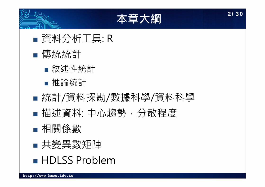
本章大綱

資料分析工具: R 傳統統計

敘述性統計推論統計

統計/資料探勘/數據科學/資料科學描述資料: 中心趨勢，分散程度相關係數共變異數矩陣 HDLSS Problem

2/30


為什麼要使用R做為資料分析工具?Why R? R is a high-quality, cross-platform, flexible, widely used open source, free

language for statistics, graphics, mathematics, and data science. R contains more than 5,000 algorithms (>10,000 packages) and millions of

users with domain knowledge worldwide.

http://www.r-project.org

TIOBE 全球程式語言排名

http://www.tiobe.com/tiobe-index/(共243種程式語言)

https://www.rstudio.com/

3/30


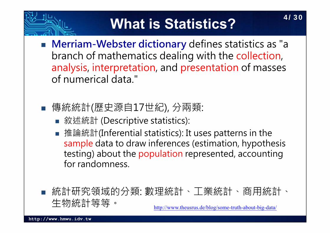
What is Statistics? Merriam-Webster dictionary defines statistics as "a

branch of mathematics dealing with the collection, analysis, interpretation, and presentation of masses of numerical data."

傳統統計(歷史源自17世紀), 分兩類: 敘述統計 (Descriptive statistics): 推論統計(Inferential statistics): It uses patterns in the

sample data to draw inferences (estimation, hypothesis testing) about the population represented, accounting for randomness.

統計研究領域的分類: 數理統計、工業統計、商用統計、生物統計等等。 http://www.theusrus.de/blog/some-truth-about-big-data/

4/30


Data Mining Diagrams

Source: Published on Nov 26, 2014Language Technologies for Geomatics: From Intelligence to AgilityPublished in: Technologyhttp://www.slideshare.net/VisionGEOMATIQUE2014/gagnon-20141112vision

Source:http://www.simplilearn.com/data-mining-vs-statistics-article

5/30


Difference between Machine Learning & Statistical Modeling

https://www.analyticsvidhya.com/blog/2015/07/difference-machine-learning-statistical-modeling/

機器學習和統計棤型的差異http://vvar.pixnet.net/blog/post/242048881為什麼統計學家、機器學習專家解決同一問題的方法差別那麼大?https://read01.com/EBPPK7.html深度 | 機器學習與統計學是互補的嗎？https://read01.com/ezQ3K.html

• Machine Learning is an algorithm that can learn from data without relying on rules-based programming.

• Statistical Modelling is the formalization of relationships between variables in the form of mathematical equations.

6/30


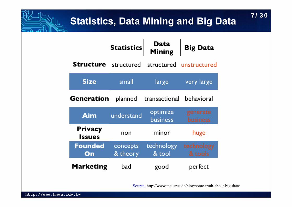
Statistics, Data Mining and Big Data

Source: http://www.theusrus.de/blog/some-truth-about-big-data/

7/30


小數據與大數據的區別調查資料

抽樣的樣本反饋的主觀的結果的結構化的斷點的

監測資料全樣的監測紀錄客觀的過程的非結構化的連續的

8/30


數據科學 Data Science

The Data Science Venn Diagramhttp://drewconway.com/zia/2013/3/26/the-data-science-venn-diagram

9/30


推薦兩本書

統計有沒有死？會不會萬歲？

只要有米倉，就會有老鼠；只要有數據，就會發展處理數據的方法。但是不是叫做統計學、或者叫做computer science 的data mining，就要看這一代的統計人如何因應變局。

趙民德，1999，「統計已死，統計萬歲！」第八屆南區統計研討會演說稿

10/30

(March 7, 2016)


Types of Data Scales Categorical (類別資料), discrete, or nominal (名目變數) — Values contain

no ordering information: 性別、種族、教育程度、宗教信仰、交通工具、音樂類型… (qualitative 屬質)

Ordinal (順序) — Values indicate order, but no arithmetic operations are meaningful (e.g., "novice", "experienced", and "expert" as designations of programmers participating in an experiment); 非常同意，同意，普通，不同意，非常不同意; 優，佳，劣。

Interval — Distances between values are meaningful, but zero point is not meaningful. (e.g., degrees Fahrenheit)

Ratio (Continuous Data 連續型資料)— Distances are meaningful and a zero point is meaningful (e.g., degrees K, 年收入、年資、身高、… (quantitative 計量)

Ordinal methods cannot be used with nominal variable Nominal methods can be used with nominal, ordinal variables.

11/30


資料描述資料中心趨勢:

平均數(average)眾數(mode)中位數(median)

資料分散程度: 四分位數(Quartile)全距(range)四分位距(interquartile range, IQR)百位數(percentile)標準差(standard deviation)變異數(variance)

https://zh.wikipedia.org/wiki/四分位距

12/30


資料描述:偏態係數偏態(skewness):

http://www.t4tutorials.com/data-skewness-in-data-mining/

大於0：右偏分配等於0：對稱分配小於0：左偏分配

13/30


資料描述:峰態係數14/30


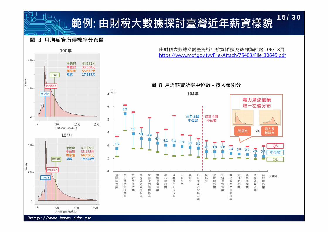
範例: 由財稅大數據探討臺灣近年薪資樣貌

由財稅大數據探討臺灣近年薪資樣貌財政部統計處 106年8月https://www.mof.gov.tw/File/Attach/75403/File_10649.pdf

15/30


玩玩看~薪情平臺

https://earnings.dgbas.gov.tw/

16/30


R程式練習: 加權算術平均數

想想看: 如何決定權重? 維度縮減方法 (e.g., PCA)

17/30


R程式練習> score2015.orig <- read.table("score2015.txt", header=T, sep = "\t")> dim(score2015.orig)[1] 80 12> head(score2015.orig)

座號學號性別姓名小考1 小考2 小考3 小考4 助教期中考期末考出席次數1 1 920541081 女高婕嘉 0 0 0 36 35 26 25 62 2 920660451 女倪儒子 30 0 NA NA 19 28 0 4...6 6 921451012 女洪銘學 35 13 20 29 55 44 40 8> summary(score2015.orig[, 3:ncol(score2015.orig)])性別姓名小考1 小考2 小考3 女:60 王彥珮 : 1 Min. : 0.00 Min. : 0.0 Min. : 0.00 男:20 王淳昀 : 1 1st Qu.:25.25 1st Qu.:10.0 1st Qu.: 20.00

王銘軒 : 1 Median :40.00 Median :30.0 Median : 40.00 朱新太 : 1 Mean :40.00 Mean :28.9 Mean : 47.76 何竣育 : 1 3rd Qu.:50.25 3rd Qu.:40.0 3rd Qu.: 80.00 余馨繁 : 1 Max. :90.00 Max. :80.0 Max. :100.00 (Other):74 NA's :4 NA's :7 NA's :13

小考4 助教期中考期末考出席次數Min. : 0.00 Min. : 0.00 Min. : 0.00 Min. : 0.00 Min. :1.0 1st Qu.: 36.00 1st Qu.: 35.00 1st Qu.: 32.00 1st Qu.: 23.75 1st Qu.:7.0 Median : 67.00 Median : 59.50 Median : 68.50 Median : 50.00 Median :8.0 Mean : 56.75 Mean : 56.24 Mean : 57.56 Mean : 46.71 Mean :7.7 3rd Qu.: 81.00 3rd Qu.: 75.25 3rd Qu.: 80.25 3rd Qu.: 69.50 3rd Qu.:9.0 Max. :100.00 Max. :100.00 Max. :100.00 Max. :100.00 Max. :9.0 NA's :15

> > table(score2015.orig["出席次數"])1 2 3 4 5 6 7 8 9 1 1 2 3 3 7 4 21 38

18/30


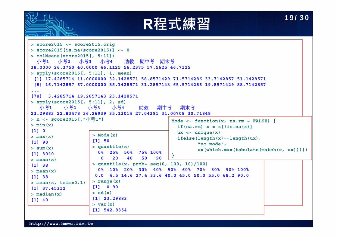
R程式練習> score2015 <- score2015.orig> score2015[is.na(score2015)] <- 0> colMeans(score2015[, 5:11])

小考1 小考2 小考3 小考4 助教期中考期末考38.0000 26.3750 40.0000 46.1125 56.2375 57.5625 46.7125 > apply(score2015[, 5:11], 1, mean)[1] 17.4285714 11.0000000 32.1428571 58.8571429 71.5714286 33.7142857 51.1428571[8] 16.7142857 67.0000000 85.1428571 31.2857143 65.5714286 19.8571429 88.7142857

...[78] 3.4285714 19.2857143 23.1428571> apply(score2015[, 5:11], 2, sd)

小考1 小考2 小考3 小考4 助教期中考期末考23.29883 22.83478 36.26939 35.13014 27.04391 31.00708 30.71848 > x <- score2015[,"小考1"]> min(x)[1] 0> max(x)[1] 90> sum(x)[1] 3040> mean(x)[1] 38> mean(x)[1] 38> mean(x, trim=0.1)[1] 37.45312> median(x)[1] 40

> Mode(x)[1] 50> quantile(x)

0% 25% 50% 75% 100% 0 20 40 50 90

> quantile(x, prob= seq(0, 100, 10)/100)0% 10% 20% 30% 40% 50% 60% 70% 80% 90% 100%

0.0 4.5 14.6 27.4 33.6 40.0 45.0 50.0 55.0 68.2 90.0 > range(x)[1] 0 90> sd(x)[1] 23.29883> var(x)[1] 542.8354

Mode <- function(x, na.rm = FALSE) {if(na.rm) x = x[!is.na(x)] ux <- unique(x)ifelse(length(x)==length(ux),

"no mode", ux[which.max(tabulate(match(x, ux)))])

}

19/30


Euclidean Distance

Pearson Correlation Coefficient

Data Matrix

Proximity Matrix

Distance and Similarity Measure 20/30


Pearson Correlation Coefficient

dist(x, method = "euclidean", diag = FALSE, upper = FALSE, p = 2)method: one of "euclidean", "maximum", "manhattan", "canberra", "binary"

or "minkowski" distance measure.cor(x, y = NULL, use = "everything",

method = c("pearson", "kendall", "spearman"))

21/30


Dissimilarity/Similarity Measure for Quantitative Data

Kendall’s tau

More Similarity Measures (1/4)

All indices range from -1 to +1

22/30


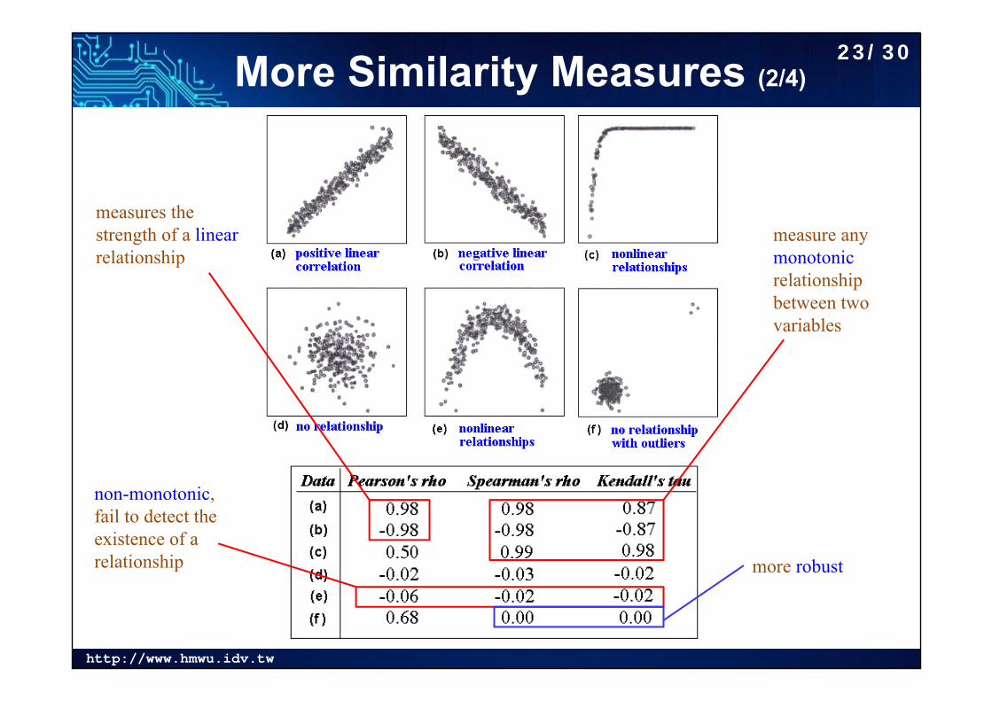
More Similarity Measures (2/4)

measures the strength of a linearrelationship

measure any monotonicrelationship between two variables

non-monotonic, fail to detect the existence of a relationship more robust

23/30


Similarity Measures for Categorical Data

2014, A survey of distance/similarity measures for categorical data, 2014 International Joint Conference on Neural Networks (IJCNN), 1907-1914.

24/30


Sample Variance-Covariance MatrixCorrelation Matrix

eigen-decomposition

25/30


High-dimensional data (HDD) Three different groups of HDD:

p is large but smaller than n; p is large and larger than p: the high-dimension low sample size data (HDLSS);

and the data are functions of a continuous variable d: the functional data.

In high dimension, the space becomes emptier as the dimension increases when p > n, the rank r of the covariance matrix S satisfies r ≤ min{p, n}. For HDLSS data, one cannot obtain more than n principal components. Either PCA needs to be adjusted, or other methods such as ICA or Projection

Pursuit could be used.

26/30


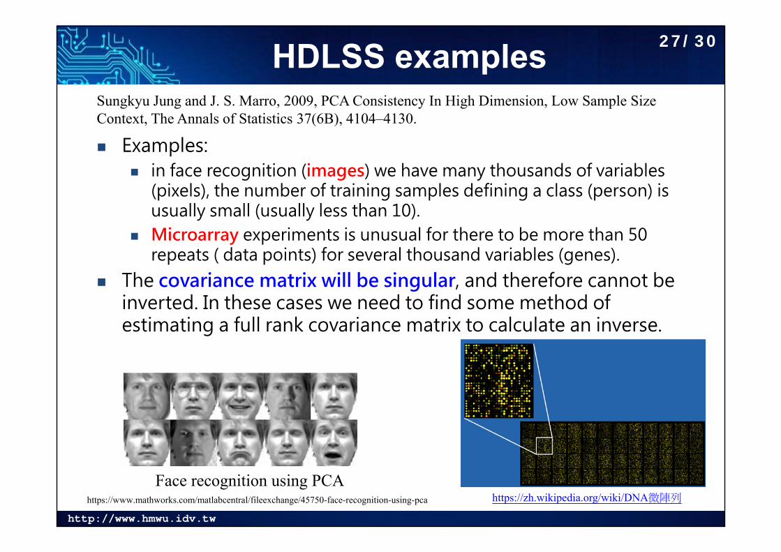
HDLSS examples

Examples: in face recognition (images) we have many thousands of variables

(pixels), the number of training samples defining a class (person) is usually small (usually less than 10).

Microarray experiments is unusual for there to be more than 50 repeats ( data points) for several thousand variables (genes).

The covariance matrix will be singular, and therefore cannot be inverted. In these cases we need to find some method of estimating a full rank covariance matrix to calculate an inverse.

Sungkyu Jung and J. S. Marro, 2009, PCA Consistency In High Dimension, Low Sample Size Context, The Annals of Statistics 37(6B), 4104–4130.

Face recognition using PCAhttps://www.mathworks.com/matlabcentral/fileexchange/45750-face-recognition-using-pca https://zh.wikipedia.org/wiki/DNA微陣列

27/30


Efficient Estimation of Covariance: a Shrinkage Approach

Schäfer, J., and K. Strimmer. 2005. A shrinkage approach to large-scale covariance matrix estimation and implications for functional genomics. Statistical Applications in Genetics and Molecular Biology . 4: 32.

google: Penalized/Regularized/Shrinkage Methods

28/30


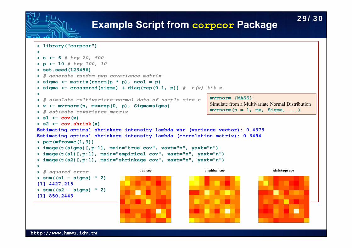
Example Script from corpcor Package

> library("corpcor")> > n <- 6 # try 20, 500> p <- 10 # try 100, 10> set.seed(123456)> # generate random pxp covariance matrix> sigma <- matrix(rnorm(p * p), ncol = p)> sigma <- crossprod(sigma) + diag(rep(0.1, p)) # t(x) %*% x> > # simulate multivariate-normal data of sample size n> x <- mvrnorm(n, mu=rep(0, p), Sigma=sigma)> # estimate covariance matrix> s1 <- cov(x)> s2 <- cov.shrink(x)Estimating optimal shrinkage intensity lambda.var (variance vector): 0.4378 Estimating optimal shrinkage intensity lambda (correlation matrix): 0.6494 > par(mfrow=c(1,3))> image(t(sigma)[,p:1], main="true cov", xaxt="n", yaxt="n")> image(t(s1)[,p:1], main="empirical cov", xaxt="n", yaxt="n")> image(t(s2)[,p:1], main="shrinkage cov", xaxt="n", yaxt="n")> > # squared error> sum((s1 - sigma) ^ 2)[1] 4427.215 > sum((s2 - sigma) ^ 2)[1] 850.2443

mvrnorm {MASS}:Simulate from a Multivariate Normal Distributionmvrnorm(n = 1, mu, Sigma, ...)

29/30


Compare Eigenvalues> # compare positive definiteness> is.positive.definite(sigma)[1] TRUE> is.positive.definite(s1)[1] FALSE> is.positive.definite(s2)[1] TRUE> > # compare ranks and condition> rc <- rbind(+ data.frame(rank.condition(sigma)), data.frame(rank.condition(s1)),+ data.frame(rank.condition(s2)))> rownames(rc) <- c("true", "empirical", "shrinkage")> rc

rank condition toltrue 10 256.35819 6.376444e-14empirical 5 Inf 1.947290e-13shrinkage 10 15.31643 1.022819e-13> >> > # compare eigenvalues> e0 <- eigen(sigma, symmetric = TRUE)$values> e1 <- eigen(s1, symmetric = TRUE)$values> e2 <- eigen(s2, symmetric = TRUE)$values> >> matplot(data.frame(e0, e1, e2), type = "l", ylab="eigenvalues", lwd=2)> legend("top", legend=c("true", "empirical", "shrinkage"), lwd=2, lty=1:3, col=1:3)

Shrinkage estimation of covariance matrix:• cov.shrink {corpcor}• shrinkcovmat.identity {ShrinkCovMat} • covEstimation {RiskPortfolios}

30/30

Documents

AI-D1-1-hmwu R BasicStat · 推薦兩本書 統計有沒有死？會不會萬歲？ 只要有米倉，就會有老鼠；只要有數 據，就會發展處理數據的方法。

AI-D1-1-hmwu R BasicStat · 推薦兩本書統計有沒有死？會不會萬歲？只要有米倉，就會有老鼠；只要有數據，就會發展處理數據的方法。