Embed Size (px)
Citation preview

Instructions for use
Title Agricultural Productivity Growth and Household Food Security Improvement in Nepal
Author(s) Morioka, Masako; Kondo, Takumi
Citation Review of development economics, 21(4), e220-e240https://doi.org/10.1111/rode.12325
Issue Date 2017-11
Doc URL http://hdl.handle.net/2115/71781
Rights
© 2017 John Wil ey & Sons Ltd., This is the peer reviewed version of the following article: Morioka, Masako &Kondo, Takumi (2017). Agricultural Productivity Growth and Household Food Security Improvement in Nepal. Reviewof development economics, 21(4), e220-e240, which has been published in final form athttps://doi.org/10.1111/rode.12325. This article may be used for non-commercial purposes in accordance with WileyTerms and Conditions for Self-Archiving
Type article (author version)
File Information foodsucuritynepal18th_figure2.pdf
Hokkaido University Collection of Scholarly and Academic Papers : HUSCAP

1
1. Introduction 1
Food security in agriculture-based countries cannot be discussed without 2
considering agricultural development (World Bank, 2007). Agriculture plays an 3
important role in the food security of developing countries, which is mostly assisted 4
by subsistence farming. 5
There are different approaches to analyzing food security: food availability, 6
income-based, basic needs, entitlement, and sustainable livelihood. The 7
income-based approach is used for analyzing poverty in developing countries and it 8
is more effective in analyzing countries operating an ideal economy. However, this 9
method is not highly reliable in low-income countries wherein subsistence 10
agriculture is dominant (Burchi and De Muro, 2015). 11
In analyzing food security in subsistent rural areas, the concept of 12
entitlement approach (Sen, 1981) is important. Entitlement includes two 13
components: (1) endowment, which is initial ownership (e.g., labor force, holding 14
land), and (2) exchange, which means that individuals can acquire alternative goods 15
through exchange with others or nature (Dreze & Sen, 1989, 10-11). Farmers can 16
produce crops by exchanging their land and labor with nature. If a farmer’s right to 17
nature is damaged by some unfavorable situation (e.g., illness, loss of employment, 18
rise in food price), it is called “entitlement failure.” Concepts such as these 19
emphasize the importance of self-sufficient agriculture in food security. 20
Improvements in agricultural productivity contribute to the reduction of 21
poverty (Datt and Ravallion, 1998; Hanmer and Naschold, 2000; Irz and Roe, 2000; 22
Irz et al., 2001; Janvry and Sadoulet, 2009; Thirtle et al., 2001; Woden, 1999; World 23
Bank, 2007). In addition, agricultural productivity influences food poverty (Block, 24
1995; Mainuddin and Kirby, 2009; Ogundari and Awokuse, 2016). 25
Agricultural productivity affects the level of poverty in Nepal (Devkota 26
and Upadhyay, 2013); however, in reaching this conclusion, labor productivity was 27
assumed as agricultural productivity. However, labor productivity measures only 28
the efficiency of labor input and disregards other production factors and 29
productivity improvement independent of physical resource inputs. 30
In this paper, we present the effect of agricultural productivity on 31
agricultural workers’ food consumption, which is a focus that has an opposite 32
relation with that of preceding studies. Considering that an increase in agricultural 33
2
output is directly connected with a farmer’s income, we cannot underestimate the 1
influence of agricultural productivity on human capital. This paper has three 2
primary aims. First, we identify the Total Factor Productivity (TFP) of agriculture 3
in Nepal as an index of overall agricultural productivity. Second, we quantify the 4
impact of agricultural production on household food security. Third, we use the 5
panel datasets of the NLSS from 1995/96 and 2003/04. Using panel data enable us 6
to eliminate heterogeneity, such as consumption patterns at the household level, 7
land condition in agricultural production, and access to markets for buying inputs 8
and selling outputs. Specifically, each household has a food consumption pattern 9
that is determined not only by its preferences but also by its level of income. 10
However, we limit the discussion of the effect of human capital on agricultural 11
productivity, as with previous research. In addition, we do not exclude landless 12
laborers, who are regarded as the poorest people in Nepal. In this paper, we 13
investigate farmers in Nepal in their entirety. 14
15
2. Overall condition in Nepal 16
Nepal is a landlocked country bordered to the north by China and to the 17
south, east, and west by India. Nepal is commonly divided into three ecological 18
belts: the Mountain belt, Hill belt, and Terai belt, in order of decreasing height 19
above sea level. The Terai belt is a fertile, humid, and flat agricultural strip. In 20
addition, Nepal is divided into five development regions that cut across these 21
ecological belts: Eastern Development Region, Central Development Region, 22
Western Development Region, Mid-Western Development Region, and Far-Western 23
Development Region. 24
A high percentage—as much as 66.5% in 2013—of the Nepalese workforce 25
is engaged in agriculture, although agriculture’s share of GDP is only about 35%. 26
This implies that agriculture remains a key economic activity and a source of basic 27
income for the majority of the population in Nepal. Meanwhile, rapid population 28
growth has caused a decline in land-holding area per person across the country, 29
except in the Mountain belt (Table 1). Of all the regions, the Far-Western 30
Development Region has exhibited the smallest land-holding size for at least the 31
past 20 years. High population density and limited cultivable area have led to 32
severe land fragmentation. Almost 75% of households have holdings of less than one 33

3
hectare, which is inadequate to meet their subsistence needs (Central Bureau of 1
Statistics [CBS], 2004). The CBS (2005) reported the average income per person 2
according to income resources between 1995 and 2003. Remittances and income 3
from non-agricultural sectors have shown an increasing trend. On the other hand, 4
income from the agricultural sector either stagnated or decreased between 1995 and 5
2003. Therefore, the agricultural sector has grown sluggishly despite being a major 6
income source for the Nepalese population. 7
The CBS (2005) reported changes in the head-count poverty ratio using 8
both cross-section and panel data collected by the NLSS carried out in 1994–95 and 9
2003–04. The cost-of-basic-needs method was used to define the poverty line. The 10
national poverty ratio in 1995–96 was estimated at about 42%, while that for 2003–11
04 was estimated at about 31%. However, the gains in poverty reduction stem from 12
urban areas. Poverty declined only 20% within rural areas, compared with a 56% 13
decline in urban areas. We can confirm the trend of substantial poverty decline in 14
Nepal, but poverty reduction is focused on only certain segments of the poor. The 15
CBS (2005) also measured the food poverty line prior to expenditure on food and 16
non-food goods because non-food expenditures tend to contain many “noisy” 17
purchases that induce measurement bias, such as the flow of durable goods, as 18
pointed out by Lanjouw and Lanjouw (2001). Therefore, food consumption might be 19
regarded as a substitute for their livelihood or the poverty ratio. 20
Moreover, the CBS (2005) reported an increase in the agricultural wage 21
rate and poverty alleviation among agricultural employed laborers. They concluded 22
that out-migration and availability of job opportunities in agricultural wage 23
employment accompanied by out-migration stimulated a rise in the agricultural 24
wage rate, which benefitted agricultural wage laborers, who tend to be the poorest 25
population segment in the Nepal. Conversely, the World Bank (2006) reported a 26
stagnation in agricultural income because of higher input costs and lower output 27
prices in the crop sector. However, neither of these reports paid particular attention 28
to agricultural growth or productivity in Nepal. 29
In this paper, we opt to use panel datasets to measure agricultural TFP 30
and estimate the impact of agricultural revenue upon household food security. We 31
choose not to measure poverty level considering both food and non-food goods 32
because the panel datasets are not only missing many values but also exclude some 33

4
education data. Nonetheless, it is difficult to compare food expenditure across 1
households because each household has a particular food consumption pattern. 2
However, we could subtract a household’s particular pattern of not only food 3
consumption but also heterogeneity caused by a household’s unique characteristics 4
or agricultural land condition. 5
Devkota and Upadhyay (2013) estimated agricultural productivity using 6
the Cobb–Douglas and translog production functions to quantify productivities’ 7
effect on poverty reduction. They then identified the determinants of agricultural 8
productivity that affect poverty reduction. They also measured productivity as 9
output per worker and determined that the translog production model fits the 10
Nepalese data better than the Cobb–Douglas model. Then, they used the translog 11
production function to investigate the impact on poverty through the determinants 12
of productivity. Their results indicate that a favorable change in the fundamental 13
determinants of crop income, such as area, fertilizers, or investments, will lead to a 14
drop in poverty. Moreover, an integrated effect from a change in all covariates of 15
productivity is larger than the effect produced by any one factor in isolation. Their 16
findings imply that policies supporting comprehensive productivity-enhancing 17
factors will lead to a decrease in poverty. However, land and labor productivity 18
depend on various factors, such as the nature of soil, land condition, level of market 19
maturity, and so on, which can be difficult to manipulate. 20
21
3. Data Sources and Methodology 22
Data 23
The data were obtained from the NLSS 1995–96 and 2003–04 (NLSS-I 24
and NLSS-II) carried out by Nepal’s CBS. NLSS-I and NLSS-II are based on 25
nationally representative surveys of households and communities that consist of 26
cross-sectional and panel datasets. This survey follows the World Bank in using the 27
Living Standard Measurements Study methodology and utilizes a two-stage sample 28
design selection method. The panel data include 962 households, which were also 29
interviewed in NLSS-I, from 95 panel Primary Sample Units. The survey’s 30
questionnaire contains broad information, including detailed income and 31
consumption data and household-specific social and economic information. 32
Households with positive numbers for crop production include 748 households in 33

5
NLSS-I and 740 households in NLSS-II. These datasets in 1995 and in 2003 do not 1
merge perfectly for several reasons: (i) the head of the household may have changed 2
because of a death in the family, working out, a household split, and so on and (ii) 3
there are single-year data related to agricultural production, because households 4
might have left or entered into agriculture production during the eight years 5
between surveys. Moreover, We have eliminated data with outlying observation. 6
Therefore, the dataset consists of 503 households, which are summarized in Table 2. 7
Table 2 shows expenditure on farming, agricultural revenue, and food 8
consumption levels for 1995 and 2003 as evaluated in 1995 values. Food 9
consumption is determined as the food expenditure per person: total household food 10
expenditure divided by number of household members converted into adults. Food 11
consumption is calculated by adding expenditures on home-produced foods, 12
purchased foods and foods received in kind. We have calculated food prices from 13
purchased foods’ expenditure divided by its amount. 14
This study does not focus especially on landless agricultural wage labors, 15
despite their being the poorest segment of the Nepalese population; this is because 16
of the employed methodology of measuring the effect of agricultural productivity via 17
food consumption. In this paper, we limit ourselves to households with positive 18
agricultural production in both 1995 and 2003. Then, we estimated the effect of 19
agricultural productivity on food consumption at the household level. 20
21
Measuring Total Factor Productivity and Regressing Food Consumption 22
TFP is the part of output that cannot be explained by the amount of inputs used in 23
production. We will show the consistency of TFP. We set output quantity vectors as 24
𝑦𝑡 ≡ (𝑦1𝑡 , … , 𝑦𝑚
𝑡 ) , where 𝑝𝑡 ≡ (𝑝1𝑡 , … , 𝑝𝑚
𝑡 ) is the output price vectors, and input 25
quantity vectors as 𝑥𝑡 ≡ (𝑥1𝑡 , … , 𝑥𝑚
𝑡 ) , where 𝑤𝑡 ≡ (𝑤1𝑡, … , 𝑤𝑚
𝑡 ) is the input price 26
vectors related to period 𝑡, for 𝑡 = 0, 1. We denote the base period as period 0 and 27
the target period as period 1. The Fisher ideal output and input quantity indices are 28
defined as 29
6
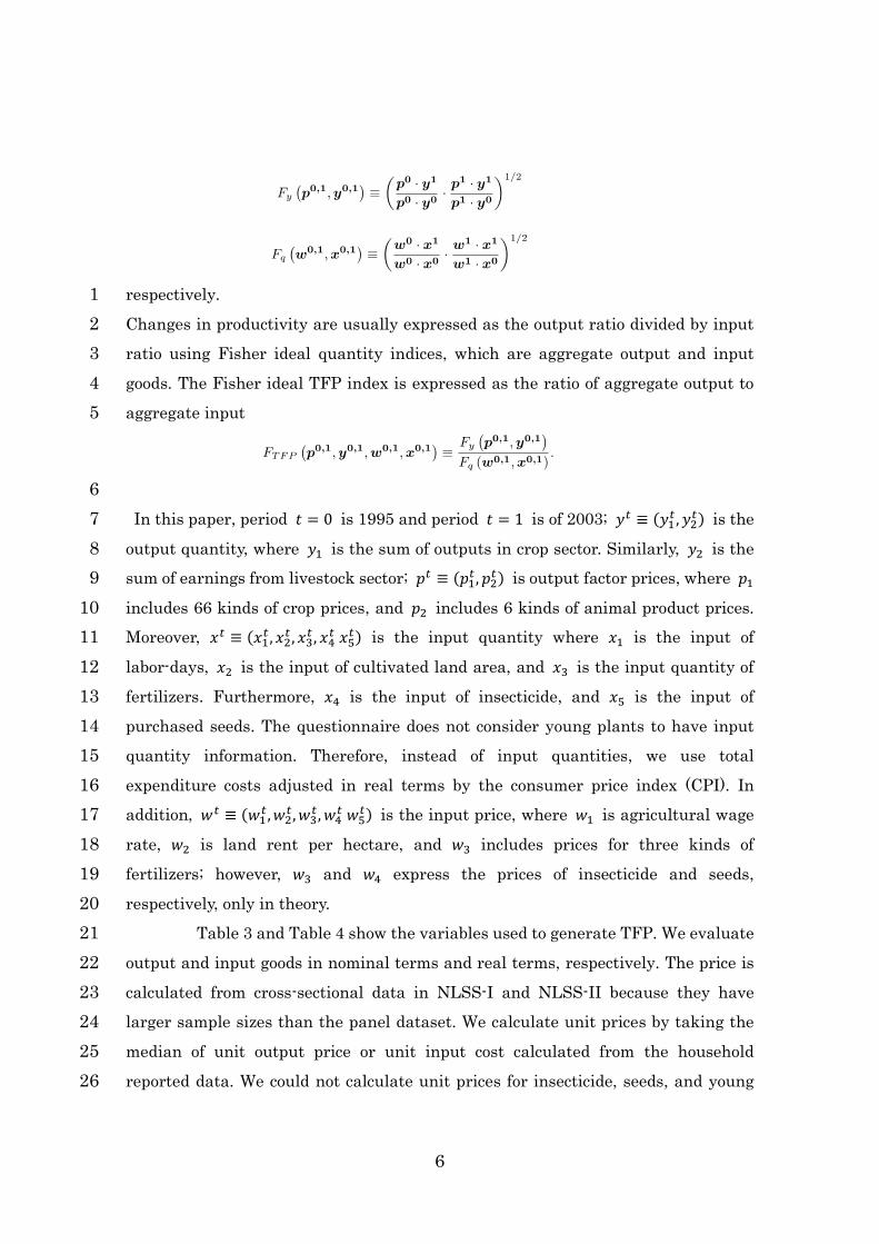
respectively. 1
Changes in productivity are usually expressed as the output ratio divided by input 2
ratio using Fisher ideal quantity indices, which are aggregate output and input 3
goods. The Fisher ideal TFP index is expressed as the ratio of aggregate output to 4
aggregate input 5
6
In this paper, period 𝑡 = 0 is 1995 and period 𝑡 = 1 is of 2003; 𝑦𝑡 ≡ (𝑦1𝑡 , 𝑦2
𝑡) is the 7
output quantity, where 𝑦1 is the sum of outputs in crop sector. Similarly, 𝑦2 is the 8
sum of earnings from livestock sector; 𝑝𝑡 ≡ (𝑝1𝑡 , 𝑝2
𝑡) is output factor prices, where 𝑝1 9
includes 66 kinds of crop prices, and 𝑝2 includes 6 kinds of animal product prices. 10
Moreover, 𝑥𝑡 ≡ (𝑥1𝑡 , 𝑥2
𝑡 , 𝑥3𝑡 , 𝑥4
𝑡 𝑥5𝑡) is the input quantity where 𝑥1 is the input of 11
labor-days, 𝑥2 is the input of cultivated land area, and 𝑥3 is the input quantity of 12
fertilizers. Furthermore, 𝑥4 is the input of insecticide, and 𝑥5 is the input of 13
purchased seeds. The questionnaire does not consider young plants to have input 14
quantity information. Therefore, instead of input quantities, we use total 15
expenditure costs adjusted in real terms by the consumer price index (CPI). In 16
addition, 𝑤𝑡 ≡ (𝑤1𝑡, 𝑤2
𝑡, 𝑤3𝑡, 𝑤4
𝑡 𝑤5𝑡) is the input price, where 𝑤1 is agricultural wage 17
rate, 𝑤2 is land rent per hectare, and 𝑤3 includes prices for three kinds of 18
fertilizers; however, 𝑤3 and 𝑤4 express the prices of insecticide and seeds, 19
respectively, only in theory. 20
Table 3 and Table 4 show the variables used to generate TFP. We evaluate 21
output and input goods in nominal terms and real terms, respectively. The price is 22
calculated from cross-sectional data in NLSS-I and NLSS-II because they have 23
larger sample sizes than the panel dataset. We calculate unit prices by taking the 24
median of unit output price or unit input cost calculated from the household 25
reported data. We could not calculate unit prices for insecticide, seeds, and young 26

7
plants, or livestock earnings from the NLSS datasets. Therefore, we used the CPI 1
reported by Nepal Rastra Bank (2006) or the price index reported from the 2
Agri-Business Promotion and Statistics Division (ABPSD, 1995–96, 2012–13) to 3
adjust prices in lieu of nominal and real prices. Crop output has been totaled for 4
each crop output and is expressed by each crop unit’s price in nominal and real 5
terms. Earnings from livestock containing meats, eggs, and some dairy products are 6
adjusted by ABPSD (1995–96, 2012–13). 7
Cultivated land area is the sum of owned, rented, mortgaged, and 8
sharecropped land area. Land rent was calculated from median land rent received 9
per hectare as reported by landlords. We then estimated the value of the cultivated 10
land area in both nominal and real terms. The value of invested labor work-days is 11
the sum of family labor and employed labor. Its unit price was derived from the 12
median of agricultural wage payments per work-days reported by employers. 13
Fertilizer was calculated using the input quantity multiplied by the unit price of 14
each fertilizer type. Fertilizer unit prices are medians of fertilizer expenditures 15
divided by purchase quantities. Insecticide, seeds, and young plants use the raw 16
expenditure data, which were then adjusted in real terms using CPI reported data 17
from Nepal Rastra Bank (2006). 18
Thus, we calculated the Fisher quantity index for both output and input. 19
Table 5 shows the details for the Fisher TFP. Comparing the log of TFP information 20
in Table 5, the Mountain and Hill belts grew approximately 20 to 30 % during the 21
specified eight years. The Western Development Regions had grown considerably 22
compared with other development regions. However, recession or no change 23
occurred in the Terai belt (–6.3%), meaning that agricultural productivity in 2003 in 24
the Terai belt is almost same as its agricultural productivity in 1995. The 25
Far-Western Development Region could be also stagnant (–2.7%). 26
This might be due to the fact that agricultural productivity in the Terai 27
belt had already risen by 1995. However, the Western and Mid-Western 28
Development Regions largely showed growth from 1995 to 2003. The high TFP 29
levels in these development regions were not influenced so much by production 30
growth for the eight specified years as by their low level of technology in 1995, since 31
the western area of Nepal lacked infrastructure development. 32
33

8
Food consumption levels and Ordinary Least Squares regression 1
The increase in TFP cannot be explained by that of input. The following 2
equation shows the Cobb–Douglas production function, 3
[equation.pdf] 4
5
"Y" is the agricultural output, "vector x" is a bundle of production factors, and "A" is 6
the TFP. Taking the log of both sides, 7
[equation.pdf]. 8
If we estimate this equation model, its intercept is the growth of TFP. Therefore, 9
using the Cobb–Douglas production function, we estimate the growth of TFP 10
between 1995 and 2003. 11
𝑡 and 𝑡 1 represent agricultural outputs in 𝑡 and 𝑡 1 terms, respectively. 12
Taking the ratio of the two terms, 13
[equation.pdf] 14
Taking the log of both sides, the equation is expressed as follows. 15
[equation.pdf] 16
represents the change in TFP. In our analysis, "Y" is the agricultural output 17
based on 1995 prices. Input goods are labor, fertilizer, pesticide, and seed. Labor is 18
measured as man-days multiplied by average wage using the 1995 prices calculated 19
from the NLSS cross section data. Fertilizer, pesticide, and seed represent the 20
expenditure in 1995 prices calculated from the NLSS cross section data. However, 21
input of fertilizer, pesticide, and seed is low; therefore, the bundle of inputs (vector 22
x) is the sum of these inputs’ real amount using 1995 prices. Dummy variables of 23
the three ecological belts and five development regions are also added. 24

9
1
We estimate the change of agricultural productivity in Nepal. We also 2
estimate the effect of agricultural production and productivity on food consumption. 3
[equations.pdf] 4
5
The change of food consumption represents the log of ratio of the two periods’ 6
expenditure on food per year, per person in 1995 prices. The food consumption 7
consists of 39 food items, the prices of which are calculated from food purchase 8
records in the NLSS’s annual cross-section data. Using these derived prices, we 9
re-evaluate food consumption quantity for each year, with the subscript denoting a 10
price for the food item for re-evaluation and the superscript indicating the quantity 11
of food consumed each year. The sum of food consumed by a household is divided by 12
household size, which in turn is converted in energy requirements for different ages 13
and genders. Family members indicate changes in household size based on nutrient 14
requirements. Income from other sources as well as the number of consumers, both 15
influence food consumption. Income is treated separately and it is divided into 16
self-employment in agriculture, other income (wage employment in agriculture and 17
non-agriculture, and self-employment in non-agriculture), and remittances. The 18
agricultural output growth represents the log of ratio of the two periods’ 19
agricultural gross revenue in 1995 prices. It serves as a proxy variable of changes in 20
proportion of agricultural output. Other income is calculated as the sum of income 21
from being wage-employed in the agricultural sector and wage income from jobs in 22
both agricultural and non-agricultural sectors. We take a difference of other income 23
and remittance in two terms because they have many zero values in each period. 24
[equations.pdf] 25

10
We consider the interaction between the food consumption level in 1995 1
and the change in income. In other words, if a household did not have sufficient food 2
in 1995, they will try to increase their income. For example, a member of the 3
household may search for work in non-agricultural sectors, migrate to other regions 4
or countries, or try to enhance the agricultural output. Income elasticity of food 5
demand is higher for the poor. Moreover, if households are provided with enough 6
food, food demand would be inelastic. In order to study the impact of agricultural 7
output growth by household in the 10th to 90th percentile values of food consumption 8
in 1995, we estimate equation (2) as follows. 9
[equations.pdf] 10
11
where 𝐹𝐶95𝑝95 − 𝑝𝑐𝑡𝑃
𝐹𝐶95𝑝95
𝑡ℎ indicates the difference between food consumption level in 12

11
1995 and Pth percentile value. Similarly, pct10th/pct25th/pct50th/pct75th/pct90th refer 1
to the corresponding percentile values in the equation. Y represents for agricultural 2
gross revenues, while FC represents food consumption. Finally, Δ defines the 3
difference between 2003 and 1995 values. 4
However, we use the two-stage least squares methods because of the 5
endogeneity of agricultural output. Further, we use the TFP estimator from Eq. (1) 6
as the instrumental variables. TFP can be likened to "manna from heaven," and is 7
generated from the exchange of nature for human activity. TFP is the adequate 8
exogenous variable for food consumption. The details of each variable are presented 9
in Table 6 and Table 7. The result of Eq. (1) is shown in Table 8. The result of the 10
first and the second stage in Eq. (2) is shown in Table 9. 11
12
4. Results 13
The row (1) in Table 8 shows the result of Eq. (1), which is the estimation 14
result for all of Nepal. It reveals that TFP had grown about 11.4% in eight years. 15
This is not much different from the value of l_TFP in Table 5. The annual rate is 16
about 1.4 % and is calculated as follows: (1+0.1139)1/8 ≈ 1.0136. The constant in 17
Table 8 (1) shows Total Factor Productivity (TFP) in Nepal. The model in Table 8 (2) 18
informs about the relative size of each region’s TFP. We confirm the same tendency 19
in Table 5: TFPs in Terai belt have declined, while TFPs in Mid– and Far–Western 20
Development Regions have increased. 21
In order to analyze the impact of agricultural output on food consumption, 22
we estimate a two–stage least–squares model using each household’s 𝑇𝐹�̂� from 23
Table 8 (1) as an instrumental variable in Table 9. When we regress the growth in 24
food consumption on the growth in agricultural gross revenue only (Table 9 (1)), the 25
impact of agricultural production is about 0.0799. As per Table 10, the average 26
growth in agricultural gross revenue between 1995 and 2003 is about 23%, implying 27
a growth in food consumption by 23% * 0.0799=1.8%. In average terms, such a 28
growth is 3.9% between 1995 and 2003. Therefore, agricultural gross revenues 29
contribute to food consumption for 1.8%/3.9% = 46% on average. Moreover, the 30
lower the income level in 1995, the higher the positive impact of agricultural 31
production on food consumption. Figure 1 shows the presumably negative 32
relationship between growth in food consumption and food consumption level in 33

12
1995. Then, using equation (2), we attempted to estimate the impact of agricultural 1
production by food consumption level in 1995. 2
By taking 1995 as the reference year, we estimate the impact of 3
agricultural production on food consumption. Specifically, Table 10 shows the 10th to 4
90th percentiles of food consumption. Then, over the range of the observed food 5
consumption levels in 1995, coefficients of agricultural output growth (i.e., log(Agr. 6
GR in 2003 / Agr. GR in 1995)) in Table 9 (2)–(6) tend to decrease. The impact of 7
average agricultural output growth on average food consumption for each percentile 8
is showed in Table 10. 9
As can be seen in Table 10 (4), the average agricultural output growth 10
contributes to about 40% of food consumption growth among households in the 10th 11
percentile. The impact over the 50th percentile is smaller, although the coefficients 12
are not significant. In other words, this result suggests that poorer households 13
achieve food consumption growth from agricultural output growth. 14
Moreover, self-consumption accounts for a large proportion of the food 15
consumption of peasants. Figure 2 and Table 11 shows the ratio of self-consumption, 16
purchase, and in-kind, to total food consumption in NLSS-I, -II, and -III’s 17
cross-section data. In this context, a farmer is defined as an individual who 18
cultivates his own land or a rented land. Farmers have a larger proportion of 19
self-consumption than non-farmers. 20
21
5. Conclusion 22
This study mainly focused on the effects of changes in agricultural 23
production on food consumption levels. However, such previous papers based on the 24
efficiency wage hypothesis have largely not considered factors explaining 25
productivity, except nutrient intake. Devkota and Upadhyay (2013) measured the 26
effect of agricultural labor productivity on poverty alleviation in Nepal. However, 27
their measurement used cross-section data, in which it is difficult to control for 28
heterogeneity. Improvements in labor productivity lead to a similar discussion on 29
improvements in inputs such as fertilizers because farmers’ production points shift 30
along the one production function they estimated. They could not consider the 31
efficiency of inputs to outputs such as TFP, in which increases are expressed in 32
shifts of the production function itself. Our paper has clarified some of the essential 33

13
effects of income elasticity by using NLSS panel data on Nepal from 1995 to 2003, 1
together with a straightforward statistical analysis using OLS. Before clarifying the 2
relationship identified in this study, we calculated the agricultural TFP in Nepal 3
and confirmed the present status of agricultural production in Nepal. We found the 4
following two points through our analysis in this paper. 5
First, the TFP of agriculture in Nepal increased between 1995 and 2003, 6
although previous surveys reported stagnation of agricultural productivity caused 7
by land fragmentation. We have calculated the Fisher TFP index, which is the 8
microscopic approach. Moreover, the TFP we estimate from the Cobb-Douglas form, 9
which is the macroscopic approach. The TFP is almost the same in both the Fisher 10
TFP or when using the Cobb-Douglas production function. 11
Second, people with lower food consumption levels are more positively 12
impacted by enhancements to agricultural production. The effect on food 13
consumption from the result of estimation may seem little; however, it is as a result 14
of the insignificant change in the food consumption level of those who had adequate 15
food in 1995. Agriculture has adequately explained food consumption. Moreover, 16
farmers’ food consumption is dependent on self-production. It is important for the 17
food security of farmers that they cultivate themselves and receive agricultural 18
products in kind. The “westward” area of Nepal is especially known to have poor 19
social and economic conditions due to political disputes. These findings highlight 20
the importance for subsistence households to enhance their agricultural production 21
or income in order to safeguard their household’s food security. 22
The analysis in this paper has some limitations and problems to be solved 23
in future studies. We need to analyze TFP itself, especially in terms of placing 24
emphasis on variations in initial conditions across environmental zones. Such an 25
analysis would reveal the factors underlying different agricultural productivity at 26
the regional level. Both the World Bank (2006) and Devkota and Upadhyay (2013) 27
report that land and labor productivity in the agricultural sector have slumped, 28
although neither study measures or estimates specific changes in agricultural 29
productivity. We expect our ongoing research using panel datasets to obtain an 30
objective picture of the present condition will reveal the factors underlying this 31
developmental trough. 32
33

14
References
Agri-Business Promotion and Statistics Division (ABPSD) 1995/96, Statistical
information on Nepalese agriculture 1995/96, Kathmandu: Ministry of Agricultural
Development.
Block, S. A., 1995. "The recovery of agricultural productivity in sub-Saharan
Africa." Food Policy, 20(5), pp. 385–405.
Burchi, F. and De Muro, P., 2016. "From food availability to nutritional capabilities:
advancing food security analysis." Food Policy, 60, pp. 10–19.
Agri-Business Promotion and Statistics Division (ABPSD) 2012/13, Statistical
information on Nepalese agriculture 2012/13, Kathmandu: Ministry of Agricultural
Development.
Central Bureau of Statistics (CBS) 2005, Poverty trends in Nepal (1995-96 and
2003-04), Kathmandu: CBS.
Datt, G. and Ravallion, M., 1998. "Farm productivity and rural poverty in India." J
Dev Stud, 34(4), pp. 62–85.
Diewert, WE 1992, "Fisher ideal output, input, and productivity indexes revisited",
J Dev Anal, 3(3), pp. 211–248.
Devkota, S & Upadhyay, M 2013, "Agricultural productivity and poverty reduction
in Nepal ", Review of Development Economics, 17(4), pp. 732–746.
Dreze, J. and Sen, A., 1989. Hunger and public action. New York: Oxford University
Press on Demand.
Hanmer, L. and Naschold, F., 2000. "Attaining the international development
targets: will growth be enough?" Dev Pol Rev, 18, pp. 11–36.
Irz, X. and Roe, T., 2000. "Can the world feed itself? Some insights from growth
theory." Agrekon, 39(4), pp. 513–528.
Irz, X. and Lin, L., Thirtle, C. and Wiggins, S., 2001. "Agricultural productivity
growth and poverty alleviation" Dev pol rev, 19(4), pp. 449–466.
Lanjouw, JO & Lanjouw, P 2001, "How to compare apples and oranges: poverty
measurement based on different definitions of consumption", Rev of Income and
Wealth, 47(1), pp. 25–42.
Mainuddin, M. and Kirby, M., 2009. "Agricultural productivity in the lower Mekong
Basin: trends and future prospects for food security" Food Security (1), pp. 71–82.

15
Nepal Rastra Bank (NRB) 2006/07. Economic Report 2006/07, Kathmandu: NRB
Ogundari, K. and Awokuse, T., 2016. Assessing the Contribution of Agricultural
Productivity to Food Security levels in Sub-Saharan African countries. Agricultural
and Applied Economics Association 2016 Annual Meeting.
Thirtle, C., Beyers, L., Lin, L., Mckenzie-Hill, V., Irz, X., Wiggins, S. and Piesse, J.,
2002. "The impacts of changes in agricultural productivity on the incidence of
poverty in developing countries", DFID report, 7946.
Wodon, Q., 1999. Growth, poverty, and inequality: a regional panel for Bangladesh
World Bank Publications.
World Bank 2006, Nepal - Resilience amidst conflict: an assessment of poverty in
Nepal, 1995-96 and 2003-04, Washington, DC: World Bank.
World Bank 2007, World Development Report 2008 : Agriculture for Development,
Washington, DC: World Bank.

16
Table 1 Population of farmers and land segmentation in Nepal
Classification 1981/82 1991/92 2001/02 1981/82 1991/92 2001/02 1981/82 1991/92 2001/02
Mountain 1097.5 1446.6 1569.8 122.6 176.8 218.7 0.112 0.122 0.139
Hill 6022.6 7747.9 8601.4 939.7 1046.2 1038.6 0.156 0.135 0.121
Terai 5757.6 7063.6 8861.2 1401.4 1374.3 1396.6 0.243 0.195 0.158
Eastern 3398.4 3712.8 4280.2 771 783.2 795.5 0.227 0.211 0.186
Central 4160.2 5061 5970.9 823.3 719.7 750.2 0.198 0.142 0.126
Western 2,635.20 3618 4009 463.6 566.4 512.1 0.176 0.157 0.128
Mid-Western 1,634.40 2242.7 2714.5 258.2 324.7 370.7 0.158 0.145 0.137
Far-Western 1049.3 1623.8 2057.8 147.6 203.3 225.4 0.141 0.125 0.110
Source: The authors prepared the table using the data from
Agricultural Monograph Final, pp. 9–10, 16–17
TABLE 1.7: CHARACTERISTICS OF POPULATION AND HOLDINGS BY ECOLOGICAL BELT, 1981/82, 1991/92 AND 2001/02
TABLE 1.8: CHARACTERISTICS OF POPULATION AND HOLDINGS BY DEVELOPMENT REGION,1981/82 TO 2001/02
TABLE 2.2: NUMBER AND AREA OF HOLDINGS BY ECOLOGICAL BELT, 1981/82,1991/92 AND 2001/02
TABLE 2.3: NUMBER AND AREA OF HOLDINGS BY DEVELOPMENT REGION, 1981/82, 1991/92AND 2001/02
No. of persons ('000) Area of land holdings ('000 ha) Segmentation
Ecological Belt
Development
Region
Table 2 Summary of an annualized farm household
Food Poverty (households)
Regions N 1995 2003 1995 2003 1995 2003 1995 2003
Kathmandu 5 14,238 15,158 15,058 16,086 3,390 4,240 4 4
Other urban area 23 12,247 14,966 18,975 29,056 5,675 5,149 6 53
Rural eastern Hill 155 23,802 22,145 19,100 19,831 5,640 4,841 33 12
Rural eastern Terai 121 24,387 26,024 34,084 33,021 5,218 5,978 7 53
Rural western Hill 136 18,054 16,367 11,051 14,637 4,626 5,434 67 8
Rural western Terai 63 27,616 27,365 33,441 38,286 6,230 5,337 4 8
Mountain 74 23,527 20,979 13,245 16,252 4,683 4,693 31 28
Hill 236 19,712 18,277 15,916 17,704 5,372 5,279 75 88
Terai 193 24,845 26,349 33,523 35,440 5,493 5,676 15 24
Nepal 503 22,243 21,772 22,279 24,296 5,317 5,345 382 121
Source: Nepal Living Standard Survey-I and -II
Note: Prices are from 1995.
We have eliminated data with Fisher index of output (Fy) less than 0.1 and more than 5, and Fisher index of input (Fq) less than 0.1 and more than 5.
Food poverty is the number of households under food poverty line from NLSS(2005, p56. Table 2.3.1)
Agricultural output (Rs.)Agricultural input (Rs.) Food expenditure (Rs.)

17
Table 3 Description of TFP components
Quantity Unit price Definition
Crops (y1)
Each median of crop unit price by
respective unit including 66 kinds of
crops. (p1)
Gross revenue of production aggregate 66 kinds of
crops. Self-consumption is also valued (NRs. 1000)
Livestock (y2)Price adjustment by price index from
ABPSD instead of calculating p2.
Gross revenue of livestock products, such as meat,
dairy products, and animal hide (NRs. 1000)
Labor man-day
(x1)
agricultural wage rate per man-day.
(w1)
Evaluated value of man-days of family labor and
hiring labor for agricultural production evaluated by
agricultural wage rate (NRs. 1000)
Cultivated area
(x2)
Median of land rented-out per ha.
(w2)
Estamated value of sum of owned land area and
rented-in land area (NRs. 1000)
Fertilizer
purchased
quantity (x3)
Each median of fertilizer price per
kg including 4 kinds of fertilizer.
(w3)
Total purchase amount of fertilizer (NRs. 1000)
Insecticide
purchased
quantity (x4)
Price adjustment by CPI instead of
calculating p4
Total purchase amount of insecticides (NRs. 1000)
Seed purchased
quantity (x5)
Price adjustment by CPI instead of
calculating p5
Total purchase amount of seeds. (NRs. 1000)
Note: The unit price is in real term.
We created the Laspeyres Paasche quantity index for both output and input.
Output
Input
The NLSS questionaire includes 67 kinds of crops. However, "other trees" is excluded because we could not calculate its price
because of data scarcity.

18
Table
4 D
etail
s of
expla
nato
ry v
ari
able
s in
the
regre
ssio
n
Bel
tD
evel
opm
ent
regio
n
Vari
able
s1995
2003
1995
2003
1995
2003
1995
2003
1995
2003
1995
2003
1995
2003
1995
2003
1995
2003
Gro
ss r
even
ue
of
pro
ducti
on (
NR
s.)
Mea
n20,8
38
22,9
58
11,9
97
15,1
76
14,5
64
16,7
31
31,9
00
33,5
56
28,7
33
31,0
98
19,2
92
18,9
07
19,4
43
21,2
63
17,9
89
26,3
49
10,5
56
14,4
17
Med
ian
13,9
89
14,7
37
7,8
43
12,4
22
10,1
43
11,4
18
24,0
85
23,9
58
21,4
14
20,4
75
13,6
94
13,8
83
12,7
91
12,5
97
10,8
90
20,1
71
4,7
27
10,6
27
StD
ev.
23,1
33
26,2
54
10,5
14
12,0
20
16,1
80
16,1
40
28,8
99
35,2
78
27,7
92
36,9
58
17,4
68
17,1
79
21,6
92
24,7
66
20,2
15
24,9
56
28,2
03
13,4
62
Gro
ss r
even
ue
of
lives
tock
(N
Rs.
)M
ean
1,4
41
1,3
38
1,2
48
1,0
76
1,3
52
973
1,6
23
1,8
84
2,2
88
1,6
33
1,6
64
1,6
53
905
980
749
1,1
65
360
405
Med
ian
00
00
00
00
700
00
00
00
00
0
StD
ev.
3,4
83
3,3
35
2,7
55
2,7
52
3,8
58
2,7
46
3,2
50
4,0
59
3,5
85
3,5
14
4,6
91
4,1
03
1,9
91
2,3
55
1,7
43
3,1
44
1,0
38
793
Lab
or
man
day
Mea
n14,6
50
15,4
98
16,4
06
16,2
80
14,1
36
13,7
32
14,6
06
17,3
57
13,4
04
18,3
49
16,9
03
15,4
70
12,8
44
13,4
97
14,4
66
15,4
40
14,7
10
12,4
96
Med
ian
12,7
70
13,9
00
15,2
20
15,7
10
12,0
90
11,8
58
12,4
50
14,6
40
11,2
40
15,1
20
15,3
40
14,6
30
9,5
20
10,9
20
12,5
13
13,7
85
13,4
30
11,6
43
StD
ev.
10,9
39
10,1
61
9,6
30
8,1
56
10,0
31
9,4
08
12,3
68
11,3
48
9,3
59
11,8
42
9,8
71
9,1
08
13,2
49
9,5
41
11,5
59
10,6
67
10,5
88
7,4
21
Cult
ivat
ed a
rea
(x2)
Mea
n6,6
75
5,2
40
6,8
12
4,3
48
5,1
14
4,1
06
8,5
31
6,9
69
10,8
48
7,8
89
4,1
51
3,7
56
5,2
47
4,7
82
6,9
37
6,0
64
7,5
03
3,2
24
Med
ian
3,9
88
3,8
93
3,3
67
3,9
88
2,6
45
3,1
91
6,5
48
5,1
14
7,1
23
6,3
70
3,0
08
3,0
08
4,1
58
3,4
57
3,5
39
5,3
09
1,7
70
2,5
26
StD
ev.
10,3
93
5,3
90
11,3
46
2,8
71
11,5
91
3,6
04
7,9
10
7,2
15
15,9
22
7,4
39
3,9
73
3,1
02
5,4
34
5,1
24
8,3
20
4,8
95
14,8
91
2,6
56
Tota
l purc
has
e am
ount
of
fert
iliz
er (
NR
s.)
Mea
n744
797
283
320
287
335
1,4
80
1,5
45
650
999
919
851
948
850
496
586
113
111
Med
ian
181
300
42
75
60
106
915
930
180
300
406
465
181
188
0150
00
StD
ev.
1,7
41
1,6
00
445
465
526
614
2,5
74
2,2
88
1,3
03
2,3
42
1,9
47
1,1
61
2,2
11
1,4
40
1,3
08
1,4
14
492
234
Tota
l purc
has
e am
ount
of
inse
ctic
ides
(N
Rs.
)M
ean
33.4
653.3
51.0
80.0
01.1
737.7
185.3
592.9
246.2
776.1
237.8
576.5
429.1
427.0
125.2
026.4
90.0
00.0
0
Med
ian
0.0
00.0
00.0
00.0
00.0
00.0
00.0
00.0
00.0
00.0
00.0
00.0
00.0
00.0
00.0
00.0
00.0
00.0
0
StD
ev.
185.8
5268.5
09.3
00.0
08.4
3149.2
0292.9
0397.8
3277.0
1339.4
7150.0
5342.8
9164.5
796.8
8124.7
0131.5
70.0
00.0
0
Tota
l purc
has
e am
ount
of
seed
s. (
NR
s.)
Mea
n140
183
25
31
174
66
142
385
323
254
71
144
114
225
73
140
12
66
Med
ian
00
00
00
0103
00
00
039
013
017
StD
ev.
719
540
77
105
976
166
422
811
1,3
26
802
237
469
423
453
204
259
62
128
N
Note
: P
rice
s ar
e fr
om
1995.
We
hav
e el
imin
ated
data
wit
h F
isher
index
of
outp
ut
(Fy)
less
than
0.1
and m
ore
than
5, and F
isher
index
of
input
(Fq)
less
than
0.1
and m
ore
than
5.
Ter
ai
East
ern
Cen
tral
Wes
tern
Mid
-Wes
tern
Far-
Wes
tern
503
74
236
193
127
165
114
55
42
Nep
al
Mounta
inH
ill

19
Table 5 Details of Fisher index of output(Fy), input (Fq), and TFP
Belt Development region
Nepal Mountain Hill Terai Eastern Central Western
Mid-
Western
Far-
Western
Fy Mean 1.45 1.64 1.51 1.31 1.23 1.34 1.33 1.88 2.37
Median 1.16 1.47 1.21 1.00 0.945 0.992 1.18 1.74 1.90
StDev. 1.05 1.11 1.10 0.938 0.884 1.02 0.887 1.09 1.34
Fq Mean 1.24 1.09 1.19 1.36 1.39 1.06 1.37 1.21 1.14
Median 1.06 1.08 0.97 1.15 1.14 0.967 1.14 1.07 0.871
StDev. 0.834 0.617 0.801 0.930 0.908 0.626 0.930 0.809 0.951
TFP Mean 1.70 2.03 1.97 1.25 1.10 1.67 1.44 2.34 3.52
Median 1.05 1.37 1.13 0.963 0.823 1.16 0.992 1.51 2.75
StDev. 2.18 2.07 2.72 1.19 0.994 2.16 1.64 3.21 3.20
log(TFP) Mean 0.113 0.326 0.191 -0.063 0.128 -0.164 0.876 0.417 -0.027
Median 0.044 0.315 0.120 -0.038 0.144 -0.194 1.011 0.409 -0.008
StDev. 0.865 0.874 0.934 0.738 0.844 0.706 0.896 0.864 0.850
N 503 74 236 193 127 165 114 55 42
Source: NLSS-I and NLSS-II
Note: We have eliminated data with Fisher index of output (Fy) less than 0.1 and more than 5, and Fisher index of input (Fq)
less than 0.1 and more than 5.

20
Table
6 D
etail
s of
inco
me
sourc
es
Bel
tD
evel
opm
ent
regio
n
Nep
al
Mounta
inH
ill
Ter
ai
East
ern
Cen
tral
Wes
tern
Mid
-Wes
tern
Far-
Wes
tern
Vari
able
s1995
2003
1995
2003
1995
2003
1995
2003
1995
2003
1995
2003
1995
2003
1995
2003
1995
2003
FC
in 1
995
Mea
n5,2
00
6,1
53
4,9
28
5,3
18
5,3
97
6,2
78
5,0
68
6,3
30
5,4
84
6,3
42
5,4
98
5,9
38
5,4
84
7,0
15
4,2
39
5,6
22
3,9
91
4,9
88
Med
ian
4,7
70
5,6
12
4,3
78
4,9
19
4,9
76
5,7
12
4,6
90
5,7
20
5,1
68
6,0
21
5,1
86
5,4
50
4,8
10
6,5
81
3,9
11
4,9
76
3,1
32
4,6
90
StD
ev.
2,3
97
2,5
77
2,5
58
2,0
37
2,5
70
2,8
20
2,0
85
2,4
02
2,0
43
2,2
62
2,4
79
2,5
86
2,5
29
3,0
22
1,8
62
2,2
43
2,6
19
1,7
75
Oth
er i
nco
me
Mea
n8,3
88
11,3
09
8,4
87
6,4
92
9,0
70
10,4
75
7,5
19
14,2
26
7,1
47
12,9
58
8,6
93
11,7
50
8,0
45
9,5
16
8,9
77
12,0
13
10,6
21
8,9
75
Med
ian
2,7
23
6,7
86
3,6
00
4,7
80
2,8
80
3,1
40
1,5
85
10,2
39
07,7
34
2,8
80
6,1
37
3,1
57
4,0
57
5,3
15
7,1
66
5,0
00
7,0
81
StD
ev.
13,6
06
18,2
72
12,0
42
8,8
39
14,4
79
18,1
98
13,0
95
20,5
44
13,5
01
23,1
05
12,3
14
19,4
77
10,8
46
14,2
83
16,8
97
15,5
75
18,6
85
9,7
20
Fam
ily m
ember
sM
ean
4.4
44.5
23.8
14.3
04.1
64.1
05.0
45.1
34.8
54.7
64.4
64.5
44.2
94.3
04.2
74.5
73.9
44.3
6
Med
ian
4.2
14.3
63.5
74.2
13.9
34.0
74.6
64.7
14.5
04.7
54.2
94.3
64.1
63.8
84.0
54.4
13.5
04.0
7
StD
ev.
1.9
92.0
21.5
81.7
71.8
41.5
92.1
62.4
02.0
51.5
21.9
02.2
91.9
02.2
61.9
71.8
02.2
41.7
6
Rem
itta
nce
sM
ean
5,5
50
9,9
17
1,8
53
2,0
48
8,8
50
11,0
72
3,0
03
11,6
24
1,6
48
9,3
21
5,2
76
8,7
43
13,7
88
14,8
57
1,9
74
7,8
49
1,1
86
6,1
47
StD
ev.
57,2
88
32,7
70
5,6
44
5,5
70
82,9
41
36,4
00
13,8
34
34,0
43
6,9
10
34,3
71
23,5
30
27,0
81
116,8
06
45,5
64
5,3
03
21,7
91
2,6
66
17,0
20
N Sourc
e:
NL
SS
-I a
nd N
LS
S-I
I
Note
: A
ll d
ata
are
esti
mat
ed f
rom
1995 v
alu
es.
All
med
ians
of
Rem
itta
nce
s ar
e ze
ro.
FC
is
short
for
food c
onsu
mpti
on p
er
year
per
pers
on.
We
hav
e el
imin
ated
data
wit
h d
lt_lo
g_F
y l
ess
than
-2 a
nd m
ore
than
2, dlt
_re
mit
les
s th
an -
40,0
00 r
upe
es a
nd m
ore
than
40,0
00 r
upe
es, F
ood95pc m
ore
than
10,0
00 r
upe
es, an
d d
lt_oth
erIN
C l
ess
than
-45,0
00 r
upe
es a
nd
more
than
45,0
00 r
upe
es.
124
66
51
548
83
255
210
132
175
21
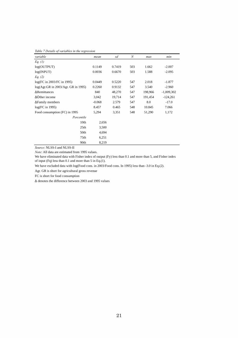
Table 7 Details of variables in the regression
variable mean sd N max min
Eq. (1)
log(OUTPUT) 0.1149 0.7419 503 1.662 -2.007
log(INPUT) 0.0036 0.6670 503 1.588 -2.095
Eq. (2)
log(FC in 2003/FC in 1995) 0.0449 0.5220 547 2.018 -1.877
log(Agr.GR in 2003/Agr. GR in 1995) 0.2260 0.9132 547 3.540 -2.960
DRemittances 840 48,270 547 198,966 -1,009,302
DOther income 3,042 19,714 547 191,454 -124,261
DFamily members -0.068 2.579 547 8.0 -17.0
log(FC in 1995) 8.457 0.465 548 10.845 7.066
Food consumption (FC) in 1995 5,294 3,351 548 51,290 1,172
Percentile
10th 2,656
25th 3,500
50th 4,694
75th 6,251
90th 8,219
Source: NLSS-I and NLSS-II
Agr. GR is short for agricultural gross revenue
FC is short for food consumption
D denotes the difference between 2003 and 1995 values
Note: All data are estimated from 1995 values.
We have eliminated data with Fisher index of output (Fy) less than 0.1 and more than 5, and Fisher index
of input (Fq) less than 0.1 and more than 5 in Eq.(1).
We have escluded data with log(Food cons. in 2003/Food cons. In 1995) less than -3.0 in Eq.(2).

22
Table 8 Estimates of TFP from residuals
log(INPUT) 0.2775 *** 0.3191 ***
[0.05] [0.05]
Hill -0.0788
[0.10]
Terai -0.1779 *
[0.10]
Central 0.1209
[0.08]
Western 0.1135
[0.09]
Mid-Western 0.4903 ***
[0.11]
Far-Western 0.7553 ***
[0.11]
constant 0.1139 *** 0.037
[0.03] [0.10]
R-squared 0.0622 0.1654
Adj-R-squared 0.0604 0.1536
N 503 503
Note: * p < 0.1, ** p < 0.05, *** p < 0.01
Values in [ ] are robust standard errors
Belt
( Base group: Mountain )
Development region
( Base group: Eastern )
We have eliminated data with Fisher index of output (Fy) less
than 0.1 and more than 5, and Fisher index of input (Fq) less
than 0.1 and more than 5.
(1) (2)
Coefficient Coefficient

23
Table 9. Relationship among food consumption, agricultural output, and other factors
(1) (2) (3) (4) (5) (6)
p10 p25 p50 p75 p90
log(Agr. GR in 2003/Agr. GR in 1995) 0.0799 *** 0.0705 *** 0.0571 *** 0.0372 ** 0.00952 -0.0281
[0.03] [0.02] [0.02] [0.02] [0.02] [0.03]
log(FC in 1995) -0.720 *** -0.720 *** -0.719 *** -0.717 *** -0.715 ***
[0.04] [0.04] [0.04] [0.04] [0.04]
DRemittances 2.33E-06 ** 2.18E-06 ** 1.96E-06 ** 1.68E-06 ** 1.33E-06 **
[0.00] [0.00] [0.00] [0.00] [0.00]
DOther income 8.59E-08 4.17E-07 8.85E-07 1.50E-06 * 2.27E-06 *
[0.00] [0.00] [0.00] [0.00] [0.00]
DFamily members -0.0249 *** -0.0249 *** -0.0250 *** -0.0250 *** -0.0251 ***
[0.01] [0.01] [0.01] [0.01] [0.01]
(FC–pct10 th)*log(Agr. GR in 2003/Agr. GR in 1995) -1.66E-05 ***
[0.00]
(FC–pct10 th)*D Remittances -1.82E-10 ***
[0.00]
(FC–pct10 th)*D Other income 3.93E-10
[0.00]
(FC–pct25 th)*log(Agr. GR in 2003/Agr. GR in 1995) -1.69E-05 ***
[0.00]
(FC–pct25 th)*D Remittances -1.82E-10 ***
[0.00]
(FC–pct25 th)*D Other income 3.93E-10
[0.00]
(FC–pct50 th)*log(Agr. GR in 2003/Agr. GR in 1995) -1.74E-05 ***
[0.00]
(FC–pct50 th)*D Remittances -1.82E-10 ***
[0.00]
(FC–pct50 th)*D Other income 3.93E-10
[0.00]
(FC–pct75 th)*log(Agr. GR in 2003/Agr. GR in 1995) -1.80E-05 ***
[0.00]
(FC–pct75 th)*D Remittances -1.82E-10 ***
[0.00]
(FC–pct75 th)*D Other income 3.93E-10
[0.00]
(FC–pct90 th)*log(Agr. GR in 2003/Agr. GR in 1995) -1.88E-05 ***
[0.00]
(FC–pct90 th)*D Remittances -1.81E-10 ***
[0.00]
(FC–pct90 th)*D Other income 3.92E-10
[0.00]
Constant 0.0268 6.11 *** 6.11 *** 6.10 *** 6.08 *** 6.07 ***
[0.02] [0.37] [0.37] [0.37] [0.37] [0.38]
R-squared 0.0195 0.4846 0.4846 0.4846 0.4846 0.4845
Adj-R-squared 0.0177 0.4769 0.4769 0.4769 0.4769 0.4769
N 547 547 547 547 547 547
Note: * p<0.1, ** p<0.05, *** p<0.01
Robust standard errors in square brackets
We have escluded data with log(Food cons. in 2003/Food cons. In 1995) less than -3.0.
Agr. GR is short for agricultural gross revenue.
FC is short for food consumption per year per person.
(FC –pct10 th/25 th/50 th/75 th/90 th) indicates the differences between food consumption in 1995 and the 10th/25th/50th/75th/90th quantile values, respectively
D denotes the difference between 2003 and 1995 values.
pct10th/25 th/50 th/75 th/90 th refers to the 10th/25th/50th/75th/90th percentiles, respectively
log(Food cons. in 2003/Food cons. in 1995)

24
Table 10. Contribution of agricultural output growth to food consumption growth
(2) (3) (4)
Average
agricultural
output growth
in 1995–2003
Average food
consumption
growth
in 1995–2003
Contribution
of agricultural
output growth
to food
consumption
growth
=(1)*(2)/(3)
Table 9 (1) 0.0799 *** 0.4631
Percentile
Table 9 (2) 10th 0.0705 *** 0.4086
Table 9 (3) 25th 0.0571 *** 0.3308
Table 9 (4) 50th 0.0372 ** 0.2153
Table 9 (5) 75th 0.00952 0.0551
Table 9 (6) 90th -0.0281 -0.1631
Note: * p<0.1, ** p<0.05, *** p<0.01
Values in (2) and (3) come from Table 7.
(1)
Coefficients of
agricultural
output growth
0.2274 0.0392
Table 11 Sum of food consumption in 1995, 2003, and 2010 (NP R)
Home production Purchase In-kind Total
NLSS-I (1995)
640,271 3,176,696 107,370 3,924,336
(16.3) (80.9) (2.7) (100.0)
33,010,626 20,693,927 1,470,393 55,174,946
(59.8) (37.5) (2.7) (100.0)
33,650,896 23,870,623 1,577,763 59,099,282
(56.9) (40.4) (2.7) (100.0)
NLSS-II (2003)
985,039 3,552,633 119,605 4,657,277
(21.2) (76.3) (2.6) (100.0)
35,936,775 28,235,178 1,171,546 65,343,499
(55.0) (43.2) (1.8) (100.0)
36,921,814 31,787,810 1,291,151 70,000,776
(52.7) (45.4) (1.8) (100.0)
NLSS-III (2010)
1,624,837 41,400,368 1,649,450 44,674,655
(3.6) (92.7) (3.7) (100.0)
46,266,050 52,715,638 2,174,149 101,155,837
(45.7) (52.1) (2.1) (100.0)
47,890,887 94,116,006 3,823,599 145,830,492
(32.8) (64.5) (2.6) (100.0)
Source: NLSS-I, NLSS-II, and NLSS-III
Non-agricultural
household (N=1,859)
Agricultural
household (N=3,971)
Total
(N=5,830)
Note: Prices are from 1995.
We have eliminated data with food consumption per year per person (nutrient) of
less than 1,000 rupees and more than 20,000 rupees.
Non-agricultural
household (N=153)
Agricultural
household (N=2,507)
Total
(N=2,660)
Non-agricultural
household (N=198)
Agricultural
household (N=2,828)
Total
(N=3,026)