Agreement-Discrepancy-Selection:Active Learning with Progressive Distribution Alignment

Mengying Fu†, Tianning Yuan†, Fang Wan†∗, Songcen Xu‡, Qixiang Ye†∗† University of Chinese Academy of Sciences, Beijing, China‡ Noah’s Ark Lab, Huawei Technologies, Shenzhen, China

{fumengying19, yuantianning19}@mails.ucas.ac.cn, xusongcen@huawei.com, {wanfang, qxye}@ucas.ac.cn

Abstract

In active learning, the ignorance of aligning unlabeled sam-ples’ distribution with that of labeled samples hinders themodel trained upon labeled samples from selecting infor-mative unlabeled samples. In this paper, we propose anagreement-discrepancy-selection (ADS) approach, and targetat unifying distribution alignment with sample selection byintroducing adversarial classifiers to the convolutional neu-ral network (CNN). Minimizing classifiers’ prediction dis-crepancy (maximizing prediction agreement) drives learn-ing CNN features to reduce the distribution bias of labeledand unlabeled samples, while maximizing classifiers’ dis-crepancy highlights informative samples. Iterative optimiza-tion of agreement and discrepancy loss calibrated with an en-tropy function drives aligning sample distributions in a pro-gressive fashion for effective active learning. Experiments onimage classification and object detection tasks demonstratethat ADS is task-agnostic, while significantly outperforms theprevious methods when the labeled sets are small.

IntroductionThe key idea behind active learning is that a machine learn-ing algorithm can achieve better performance with fewertraining labels if it is allowed to choose the data it wants tolearn from. Despite of the rapid progress of learning meth-ods with less supervision, e.g., weakly supervised learningand semi-supervised learning, active learning remains thecornerstone of many artificial intelligence applications forits simplicity and higher performance bound.

The majority of previous researches suggests that activelearning is an empirical method which generalizes mod-els trained on a labeled set to an unlabeled set by iterativesample selection. Uncertainty-based methods define variousmetrics to select informative samples to adapt the trainedmodel to the unlabeled set (Gal, Islam, and Ghahramani2017). Distribution-based approaches aim at estimating thelayout of unlabeled samples for selecting samples of largediversity or loss. Expected model change methods (Freytag,Rodner, and Denzler 2014; Kading et al. 2016) find out sam-ples which can cause the greatest change to the model pa-rameters or prediction samples’ loss (Yoo and Kweon 2019).

∗Correspond author.Copyright c© 2021, Association for the Advancement of ArtificialIntelligence (www.aaai.org). All rights reserved.

AgreementADS Train

EasyUnlabeled

Labeled

ADS Select

dog cowcat

cowdog cat

Hard

dog cowcat

Discrepancy

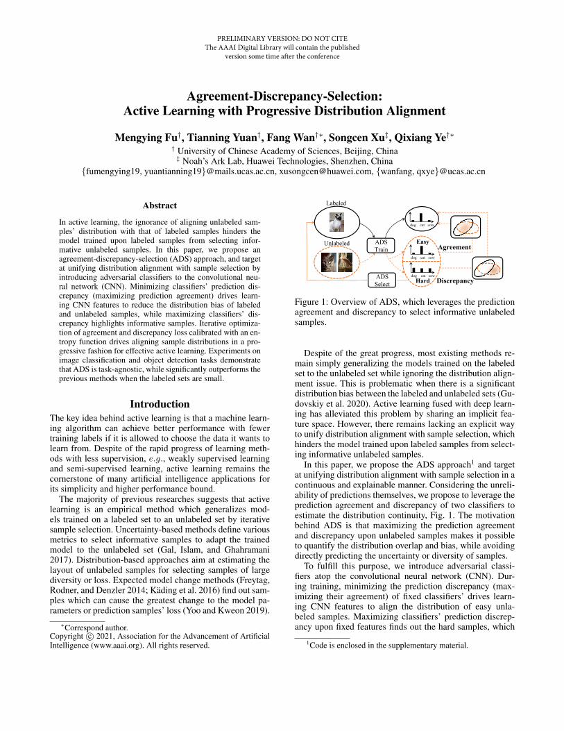
Figure 1: Overview of ADS, which leverages the predictionagreement and discrepancy to select informative unlabeledsamples.

Despite of the great progress, most existing methods re-main simply generalizing the models trained on the labeledset to the unlabeled set while ignoring the distribution align-ment issue. This is problematic when there is a significantdistribution bias between the labeled and unlabeled sets (Gu-dovskiy et al. 2020). Active learning fused with deep learn-ing has alleviated this problem by sharing an implicit fea-ture space. However, there remains lacking an explicit wayto unify distribution alignment with sample selection, whichhinders the model trained upon labeled samples from select-ing informative unlabeled samples.

In this paper, we propose the ADS approach1 and targetat unifying distribution alignment with sample selection in acontinuous and explainable manner. Considering the unreli-ability of predictions themselves, we propose to leverage theprediction agreement and discrepancy of two classifiers toestimate the distribution continuity, Fig. 1. The motivationbehind ADS is that maximizing the prediction agreementand discrepancy upon unlabeled samples makes it possibleto quantify the distribution overlap and bias, while avoidingdirectly predicting the uncertainty or diversity of samples.

To fulfill this purpose, we introduce adversarial classi-fiers atop the convolutional neural network (CNN). Dur-ing training, minimizing the prediction discrepancy (max-imizing their agreement) of fixed classifiers’ drives learn-ing CNN features to align the distribution of easy unla-beled samples. Maximizing classifiers’ prediction discrep-ancy upon fixed features finds out the hard samples, which

1Code is enclosed in the supplementary material.

PRELIMINARY VERSION: DO NOT CITE The AAAI Digital Library will contain the published

version some time after the conference

Labeled

Set Update

Classifier1

Classifier2

Label Set Training

Classifier1

Classifier2

Prediction Agreement

Classifier1

Classifier2

Prediction Discrepancy

Classifier2

Classifier1

Aligned DistributionSample Selection

Class 1 Class 2 Sample of Class 1 Sample of Class 2 Selected Sample Labeled Unlabeled

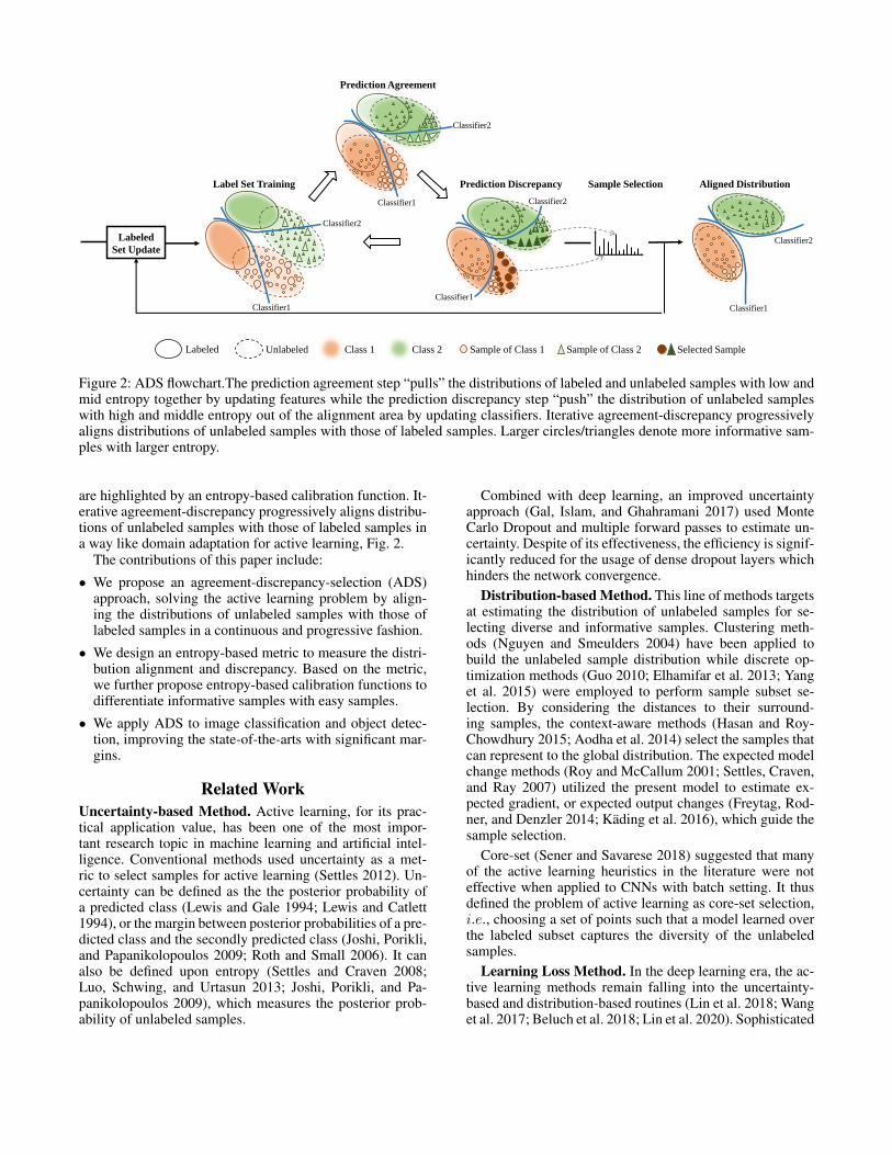
Figure 2: ADS flowchart.The prediction agreement step “pulls” the distributions of labeled and unlabeled samples with low andmid entropy together by updating features while the prediction discrepancy step “push” the distribution of unlabeled sampleswith high and middle entropy out of the alignment area by updating classifiers. Iterative agreement-discrepancy progressivelyaligns distributions of unlabeled samples with those of labeled samples. Larger circles/triangles denote more informative sam-ples with larger entropy.

are highlighted by an entropy-based calibration function. It-erative agreement-discrepancy progressively aligns distribu-tions of unlabeled samples with those of labeled samples ina way like domain adaptation for active learning, Fig. 2.

The contributions of this paper include:

• We propose an agreement-discrepancy-selection (ADS)approach, solving the active learning problem by align-ing the distributions of unlabeled samples with those oflabeled samples in a continuous and progressive fashion.

• We design an entropy-based metric to measure the distri-bution alignment and discrepancy. Based on the metric,we further propose entropy-based calibration functions todifferentiate informative samples with easy samples.

• We apply ADS to image classification and object detec-tion, improving the state-of-the-arts with significant mar-gins.

Related WorkUncertainty-based Method. Active learning, for its prac-tical application value, has been one of the most impor-tant research topic in machine learning and artificial intel-ligence. Conventional methods used uncertainty as a met-ric to select samples for active learning (Settles 2012). Un-certainty can be defined as the the posterior probability ofa predicted class (Lewis and Gale 1994; Lewis and Catlett1994), or the margin between posterior probabilities of a pre-dicted class and the secondly predicted class (Joshi, Porikli,and Papanikolopoulos 2009; Roth and Small 2006). It canalso be defined upon entropy (Settles and Craven 2008;Luo, Schwing, and Urtasun 2013; Joshi, Porikli, and Pa-panikolopoulos 2009), which measures the posterior prob-ability of unlabeled samples.

Combined with deep learning, an improved uncertaintyapproach (Gal, Islam, and Ghahramani 2017) used MonteCarlo Dropout and multiple forward passes to estimate un-certainty. Despite of its effectiveness, the efficiency is signif-icantly reduced for the usage of dense dropout layers whichhinders the network convergence.

Distribution-based Method. This line of methods targetsat estimating the distribution of unlabeled samples for se-lecting diverse and informative samples. Clustering meth-ods (Nguyen and Smeulders 2004) have been applied tobuild the unlabeled sample distribution while discrete op-timization methods (Guo 2010; Elhamifar et al. 2013; Yanget al. 2015) were employed to perform sample subset se-lection. By considering the distances to their surround-ing samples, the context-aware methods (Hasan and Roy-Chowdhury 2015; Aodha et al. 2014) select the samples thatcan represent to the global distribution. The expected modelchange methods (Roy and McCallum 2001; Settles, Craven,and Ray 2007) utilized the present model to estimate ex-pected gradient, or expected output changes (Freytag, Rod-ner, and Denzler 2014; Kading et al. 2016), which guide thesample selection.

Core-set (Sener and Savarese 2018) suggested that manyof the active learning heuristics in the literature were noteffective when applied to CNNs with batch setting. It thusdefined the problem of active learning as core-set selection,i.e., choosing a set of points such that a model learned overthe labeled subset captures the diversity of the unlabeledsamples.

Learning Loss Method. In the deep learning era, the ac-tive learning methods remain falling into the uncertainty-based and distribution-based routines (Lin et al. 2018; Wanget al. 2017; Beluch et al. 2018; Lin et al. 2020). Sophisticated

methods have extended active learning to open sets (Liuand Huang 2019), or combined it with self-paced learn-ing (Tang and Huang 2019). Nevertheless, it remains ques-tionable whether or not the intermediate feature representa-tion is effective for sample selection. Recent learning lossapproach (Yoo and Kweon 2019) can be categorized to ei-ther an uncertainty-based or a distribution-based approach.By introducing the network structure to predict the “loss” ofunlabeled samples, it estimates sample uncertainty and dis-tribution, and selects samples of large “loss” in a fashion likehard negative mining.

Despite of the great progress, the continuous distributionof labeled and unlabeled samples remain not well modeled,which causes the gap between trained model and the unla-beled samples to be predicted. Recent active learning com-bined with self-supervised learning provided an interestingsolution, but is difficult to be extended to other tasks likeobject detection (Gudovskiy et al. 2020). Motivated by themodel ensemble method (Beluch et al. 2018), our studysolves this problem by iterative prediction agreement anddiscrepancy (Saito et al. 2018). Our work is also inspiredby the uncertainty-aware graph Gaussian process (Liu et al.2020) which models continuous distribution with graph. Thedifference between our approach the adversarial learning ap-proaches (Sinha, Ebrahimi, and Darrell 2019; Zhang et al.2020) lies in that they learn how to discriminate betweensample dissimilarities in the latent space while we focus onmodeling the predictions upon unlabeled samples.

The Proposed ApproachThe core of ADS is leveraging the prediction agreement anddiscrepancy of adversarial classifiers to estimate the distri-bution of unlabeled samples. In each training iteration, threesteps are successively performed: (1) Training the backbonenetwork (feature extractor) and the classifiers using the la-beled set; (2) Fixing the classifiers, fine-tuning the featureextractor to maximize the prediction agreement (i.e., to min-imize the prediction discrepancy) on the unlabeled set toalign the distributions of unlabeled samples with those oflabeled samples; (3) Fixing the feature extractor, fine-tuningthe classifiers to maximize the prediction discrepancy on theunlabeled set and highlight informative samples. After eachtraining iteration, an entropy-based metric is used to selectinformative samples, which will be used to update the labelset for the next iteration of active learning, Fig. 2.

Label Set TrainingLet L denotes the labeled set, U the unlabeled set, and C thenumber of classes. A sample xl ∈ RH∗W∗3 from the L hasthe label yl. To quantify the distribution bias and distributionalignment between L and U , we introduce two adversarialclassifiers after the last convolutional layer, Fig. 3(a), whereg denotes the feature extractor parameterized by θg , and f1and f2 are two adversarial classifiers parameterized by θf1and θf2 , respectively.

Given the labeled set L, the purpose of network trainingis to optimize both θg and θf1 and θf2 by minimizing theBinary Cross Entropy (BCE) loss using the Stochastic Gra-

lx

g

1f 2f

l l

1

ly 2

ly

g

1f 2f

ux

Fix

1

uy 2

uy

g

uxlx

1f 2f

l l

Fix

da

Figure 3: Network architectures. (a) Label set training. (b)Prediction agreement. (c) Prediction discrepancy.

dient Descent (SGD) algorithm, as

argminθg,θf1 ,θf2

Ll(y1l , y2l )

= −C∑c=1

(yl,clogy1l,c + (1− yl,c)log(1− y1l,c)

+yl,clogy2l,c + (1− yl,c)log(1− y2l,c)).

(1)

Given an unlabeled sample for test, the network with twoadversarial classifiers takes xu as input and generates twopredictions, y1u and y2u, where y1u = f1(g(xu)) and y2u =f2(g(xu)), yu ∈ [0, 1].

When there is a significant distribution bias between Land U , unlabeled samples in the biased regions are difficultto be classified by the models trained on the labeled set. Inprevious studies, samples were selected by empirically de-signed metrics to handle the bias. However, when the biasis significant, the model experience difficulty to preciselypredict the classification probability of unlabeled samples,which could waste the quota for labeling. In what follows,the prediction agreement and prediction discrepancy mod-ules are proposed to solve this problem.

Prediction Agreement: Distribution AlignmentTo select informative samples from the unlabeled set usingthe model trained on the labeled set, the key is to find a rea-sonable way to reduce the distribution bias and increase dis-tribution alignment between labeled and unlabeled samples.To this end, we proposed a method to update the networkparameters and the feature representation so that the pre-diction agreement of f1 and f2 upon unlabeled samples ismaximized. By forcing the two classifiers to agree with eachother on predictions, the feature representation is updated sothat some unlabeled samples can “move” towards L in thefeature space, Fig. 2. The unlabeled samples “staying” inthe biased regions are considered informative and selectedfor labelling.

Particularly, each sample xu ∈ RH∗W∗3 from the un-labeled set is taken as the input of the network to predict

classification outputs, Fig. 3(b). This is an efficient infer-ence procedure given network parameters trained on the la-beled set. The adversarial classifiers f1 and f2 are both usedin the forward propagation to predict classification results.When performing back-propagation, the parameters θf1 andθf2 of the classifiers are fixed so that solely the parameters θgof the feature extractor are fine-tuned. This actually definesa procedure to update the feature space for sample align-ment, when the parameters θg of the feature extractor areoptimized by minimizing the prediction agreement loss, as

argminθg

La′(y1u, y2u) =1

C

C∑c=1

∣∣y1u,c − y2u,c∣∣ , (2)

where y1u,c and y2u,c are the predictions of the sample xu,coutput by f1 and f2, respectively.

To qualify the prediction alignment, we propose anentropy-based metric, E(u), which is defined as the meanentropy based on the classifiers’ predictions, as

E(u) = −1

2(

C∑c=1

y1u,clogy1u,c +

C∑c=1

y2u,clogy2u,c), (3)

where y1u,c and y2u,c respectively denote the prediction prob-ability of the c-th class by f1 and f2 on the unlabeled set.The entropy assigns each unlabeled sample a weight indicat-ing how well it aligns with the labeled set, providing a wayto measure the distribution alignment. Based on the entropy,a calibration weight is designed to differentiate the sampleswith large entropy from those with small entropy. Consider-ing that entropy is non-negative while the Sigmoid functionused by f1 and f2 has the largest slope near the origin, weuse the Sigmoid function to calculate the calibration weightwa, as

wa =1

n

(1− δ(E(u)− τ)

), (4)

where n denotes the batch size and δ(x) = 11+e−x the Sig-

moid function. τ is a hyper-parameter, which is experimen-tally set to 0.1.

According to Eq. 4, we assign larger alignment weightsto the samples with smaller entropy, and smaller alignmentweights to the samples with larger entropy. The advantagesof entropy calibration are two-folds: (1) It prevents hardsamples from alignment process and avoid the negative ef-fect of them on feature learning; (2) By selecting easy sam-ples but leaving hard samples out, the distance between easysamples and hard samples is further enlarged, which facil-itates highlighting the hard samples. These advantages areshown in the last three rows of Tab. 1. Accordingly, the pre-diction agreement is implemented by minimizing the cali-brated loss La to optimize the network parameters, as

argminθg

La = waLa′(y1u, y2u). (5)

Prediction Discrepancy: Highlighting InformativeSamplesBy maximizing the prediction agreement, L and U arealigned in the feature space as much as possible. In the fol-

Algorithm 1: ADS Training Procedure1 Require: Network parameters θg , classifiers’

parameters θf1 and θf2 , labeled set L and unlabeledset U .

2 for iteration do3 for epoch do4 if epoch == 0 then5 Training on L using Eq. 1;6 Compute the calibration weight wa;7 Maximize prediction agreement upon U

using Eq. 5;8 Compute the calibration weight wd;9 Maximize prediction discrepancy on U and L

using Eq. 8 and Eq. 1;10 Training on L using Eq. 1;11 Select samples using the entropy metric, Eq. 3;12 update L and U .

lowing step, we propose to maximize the discrepancy of pre-dictions to highlight informative unlabeled samples, Fig. 2.

Particularly, we fix the feature extractor’s parameters θgand fine-tune the classifiers’ parameters θf1 and θf2 to mini-mize a discrepancy loss, Fig. 3(c). The fine-tuning proceduredrives the two classifiers, f1 and f2, to output discrepant pre-dictions on each unlabeled sample xu,c, as

argminθf1 ,θf2

Ld′(y1u, y2u) = 1− 1

C

C∑c=1

∣∣y1u,c − y2u,c∣∣ , (6)

where y1u,c and y2u,c are the predictions of classifier f1 andf2 of the unlabeled sample xu,c. When optimizing Eq. 6, itrequires to simultaneously minimize the classification lossdefined in Eq. 1 to prevent the performance degradation onthe labeled samples. The loss of labeled examples and unla-beled examples are mixed together and train the model once.

Under the constraint of discrepancy loss, not all sampleshave discrepant predictions, i.e., some easy samples remainoutputting similar predictions. We design a discrepancy cal-ibration weight to handle them. Considering that smaller en-tropy means smaller prediction discrepancy, the discrepancycalibration weight wd is defined as

wd =1

n(δ(E(u)− τ)), (7)

where E(u) follows Eq. 3 on the prediction of the currentepoch. The prediction discrepancy is implemented by opti-mizing the calibrated discrepancy loss Ld, as

argminθf1 ,θf2

Ld = wdLd′(y1u, y2u). (8)

Entropy-based Sample SelectionAfter each iteration with multiple epochs of training, a smallproportion of samples staying in the bias distribution regionwould be informative samples to be selected. To quantifyhow informative each sample is, we propose the entropy-based sample selection metric,E(u), following Eq. 3, which

is based on the fact that larger entropy implies larger uncer-tainty of probabilistic predictions. The selected samples willbe added to the labeled samples for next iteration of activelearning, Fig. 2.

The learning procedure (described in Alg. 1) of ADS is anadversarial min-max discrepancy procedure, which aims toprogressively push the unlabeled distribution towards the la-beled distribution by leveraging their overlap and bias. Thisis like a kind of continuous domain adaptation where the“source” domain is the labeled samples and the “target” do-main is the unlabeled samples. During the learning proce-dure, by using the calibration weights to highlight informa-tive samples and filter out easy samples, the major propor-tion of unlabeled samples are aligned with the labeled sam-ples.

ExperimentsWe evaluate the proposed approach upon image classifica-tion and object detection tasks. In experiments, a labeleddatasetL0

k is initialized by randomly sampling k0 data pointsfrom the whole dataset UN , where N denotes the number ofsamples. In the i-th iteration of active learning, we add kilabeled samples to the labeled set and then re-train the net-work. To report the mean and standard deviation of perfor-mance, the experiment repeats for three times.

Experimental SettingsDataset. The commonly used CIFAR-10 and CIFAR-100datasets are used in the image classification task, follow-ing the experimental settings (Yoo and Kweon 2019; Sinha,Ebrahimi, and Darrell 2019; Zhang et al. 2020). CIFAR-10consists of 60000 images of 32×32×3 pixels. The trainingand test sets contain 50000 and 10000 images, respectively.CIFAR-100 is a fine-grained dataset, which consists of 100categories containing 600 images each.

Training Settings. We respectively use ResNet-18 (Heet al. 2016) and VGG-16 (Simonyan and Zisserman 2015)as backbone networks by removing the fully-connected (FC)layers and adding two classifiers atop the backbone networkto implement ADS. Considering the budget of the labeledset, we set k0=1000 and ki=1000 when using ResNet-18on CIFAR-10 while set k0=5000 and ki=2500 when usingResNet-18 on CIFAR-100 or using VGG-16. Data augmen-tation strategies including 32 × 32 random image crop andrandom image horizontal flip. The images are normalizedusing the channel mean and standard deviation vectors esti-mated over the training set.

For each learning iteration, we train the model for 200epochs with the mini-batch size 128 and the initial learningrate 0.1. After 160 epochs, the learning rate decrease to 0.01.The momentum and the weight decay are respectively set to0.9 and 0.0005.

Sub-set Sampling. The training set is regarded as theinitial unlabeled set UN , where N=50000 denote the sam-ple number. According to (Settles 2012; Sener and Savarese2018), selecting top-ki samples from UN directly is inef-ficient because of the information overlap among images.To tackle this issue, we follow the settings in (Beluch et al.

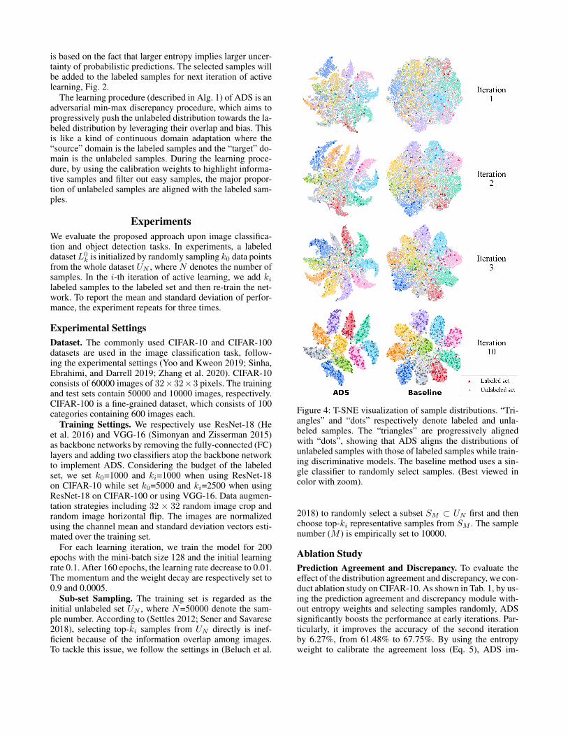
Figure 4: T-SNE visualization of sample distributions. “Tri-angles” and “dots” respectively denote labeled and unla-beled samples. The “triangles” are progressively alignedwith “dots”, showing that ADS aligns the distributions ofunlabeled samples with those of labeled samples while train-ing discriminative models. The baseline method uses a sin-gle classifier to randomly select samples. (Best viewed incolor with zoom).

2018) to randomly select a subset SM ⊂ UN first and thenchoose top-ki representative samples from SM . The samplenumber (M ) is empirically set to 10000.

Ablation StudyPrediction Agreement and Discrepancy. To evaluate theeffect of the distribution agreement and discrepancy, we con-duct ablation study on CIFAR-10. As shown in Tab. 1, by us-ing the prediction agreement and discrepancy module with-out entropy weights and selecting samples randomly, ADSsignificantly boosts the performance at early iterations. Par-ticularly, it improves the accuracy of the second iterationby 6.27%, from 61.48% to 67.75%. By using the entropyweight to calibrate the agreement loss (Eq. 5), ADS im-

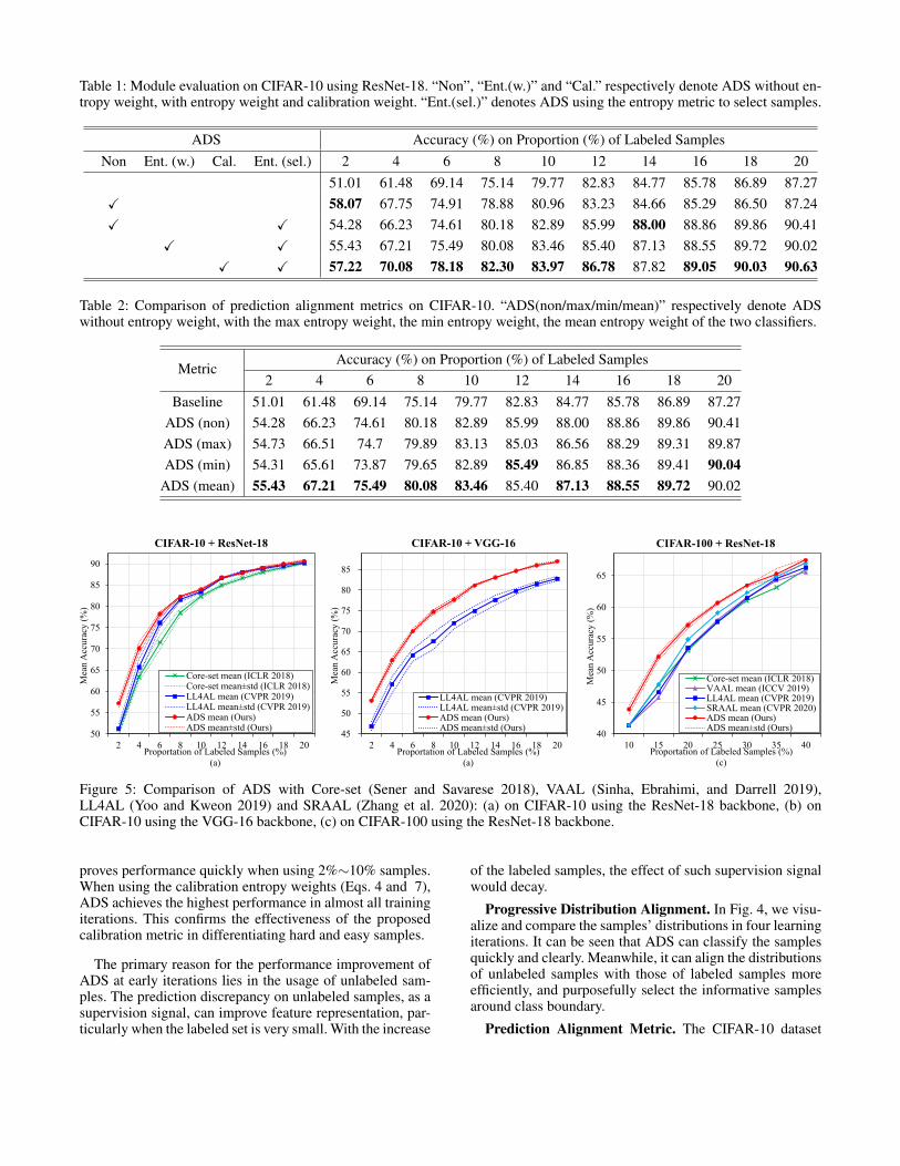
Table 1: Module evaluation on CIFAR-10 using ResNet-18. “Non”, “Ent.(w.)” and “Cal.” respectively denote ADS without en-tropy weight, with entropy weight and calibration weight. “Ent.(sel.)” denotes ADS using the entropy metric to select samples.

ADS Accuracy (%) on Proportion (%) of Labeled SamplesNon Ent. (w.) Cal. Ent. (sel.) 2 4 6 8 10 12 14 16 18 20

51.01 61.48 69.14 75.14 79.77 82.83 84.77 85.78 86.89 87.27X 58.07 67.75 74.91 78.88 80.96 83.23 84.66 85.29 86.50 87.24X X 54.28 66.23 74.61 80.18 82.89 85.99 88.00 88.86 89.86 90.41

X X 55.43 67.21 75.49 80.08 83.46 85.40 87.13 88.55 89.72 90.02X X 57.22 70.08 78.18 82.30 83.97 86.78 87.82 89.05 90.03 90.63

Table 2: Comparison of prediction alignment metrics on CIFAR-10. “ADS(non/max/min/mean)” respectively denote ADSwithout entropy weight, with the max entropy weight, the min entropy weight, the mean entropy weight of the two classifiers.

MetricAccuracy (%) on Proportion (%) of Labeled Samples

2 4 6 8 10 12 14 16 18 20Baseline 51.01 61.48 69.14 75.14 79.77 82.83 84.77 85.78 86.89 87.27

ADS (non) 54.28 66.23 74.61 80.18 82.89 85.99 88.00 88.86 89.86 90.41ADS (max) 54.73 66.51 74.7 79.89 83.13 85.03 86.56 88.29 89.31 89.87ADS (min) 54.31 65.61 73.87 79.65 82.89 85.49 86.85 88.36 89.41 90.04

ADS (mean) 55.43 67.21 75.49 80.08 83.46 85.40 87.13 88.55 89.72 90.02

50

55

60

65

70

75

80

85

90

2 4 6 8 10 12 14 16 18 20

Mea

n A

ccura

cy (

%)

Proportation of Labeled Samples (%)

(a)

CIFAR-10 + ResNet-18

Core-set mean (ICLR 2018)Core-set mean±std (ICLR 2018)LL4AL mean (CVPR 2019)LL4AL mean±std (CVPR 2019)ADS mean (Ours)ADS mean±std (Ours)

40

45

50

55

60

65

10 15 20 25 30 35 40

Mea

n A

ccura

cy (

%)

Proportation of Labeled Samples (%)

(c)

CIFAR-100 + ResNet-18

Core-set mean (ICLR 2018)VAAL mean (ICCV 2019)LL4AL mean (CVPR 2019)SRAAL mean (CVPR 2020)ADS mean (Ours)ADS mean±std (Ours)

50

60

70

80

90

2 4 6 8 10 12 14 16 18 20

Mea

n A

ccura

cy (

%)

Proportation of Labeled Samples (%)

(a)

CIFAR-10

Core-set mean (ICLR 2018)Core-set mean±std (ICLR 2018)VAAL mean (ICCV 2019)LL4AL mean (CVPR 2019)LL4AL mean±std (CVPR 2019)SRAAL mean (CVPR 2020)ADS mean (Ours)ADS mean±std (Ours)

40

45

50

55

60

65

10 15 20 25 30 35 40

Mea

n A

ccura

cy (

%)

Proportation of Labeled Samples (%)

(b)

CIFAR-100

Core-set mean (ICLR 2018)VAAL mean (ICCV 2019)LL4AL mean (CVPR 2019)SRAAL mean (CVPR 2020)ADS mean (Ours)ADS mean±std (Ours)

50

55

60

65

70

75

1k 2k 3k 4k 5k 6k 7k 8k 9k 10k

mA

P (

%)

Number of Labeled Samples

(c)

PASCAL VOC 07+12

Core-set (ICLR 2018)LL4AL (CVPR 2019)ADS (Ours)

45

50

55

60

65

70

75

80

85

2 4 6 8 10 12 14 16 18 20

Mea

n A

ccura

cy (

%)

Proportation of Labeled Samples (%)

(a)

CIFAR-10 + VGG-16

LL4AL mean (CVPR 2019)LL4AL mean±std (CVPR 2019)ADS mean (Ours)ADS mean±std (Ours)

Figure 5: Comparison of ADS with Core-set (Sener and Savarese 2018), VAAL (Sinha, Ebrahimi, and Darrell 2019),LL4AL (Yoo and Kweon 2019) and SRAAL (Zhang et al. 2020): (a) on CIFAR-10 using the ResNet-18 backbone, (b) onCIFAR-10 using the VGG-16 backbone, (c) on CIFAR-100 using the ResNet-18 backbone.

proves performance quickly when using 2%∼10% samples.When using the calibration entropy weights (Eqs. 4 and 7),ADS achieves the highest performance in almost all trainingiterations. This confirms the effectiveness of the proposedcalibration metric in differentiating hard and easy samples.

The primary reason for the performance improvement ofADS at early iterations lies in the usage of unlabeled sam-ples. The prediction discrepancy on unlabeled samples, as asupervision signal, can improve feature representation, par-ticularly when the labeled set is very small. With the increase

of the labeled samples, the effect of such supervision signalwould decay.

Progressive Distribution Alignment. In Fig. 4, we visu-alize and compare the samples’ distributions in four learningiterations. It can be seen that ADS can classify the samplesquickly and clearly. Meanwhile, it can align the distributionsof unlabeled samples with those of labeled samples moreefficiently, and purposefully select the informative samplesaround class boundary.

Prediction Alignment Metric. The CIFAR-10 dataset

50

55

60

65

70

75

1k 2k 3k 4k 5k 6k 7k 8k 9k 10k

mA

P (

%)

Number of Labeled Samples

Core-set (ICLR 2018)LL4AL (CVPR 2019)ADS (Ours)

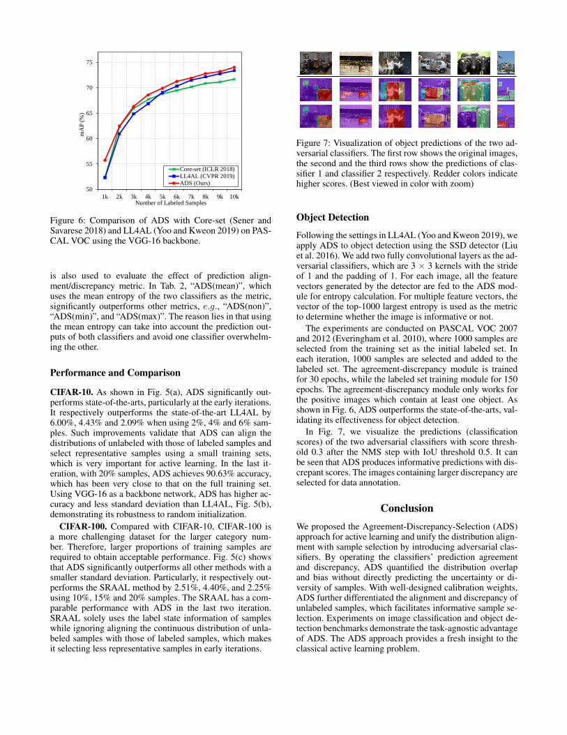
Figure 6: Comparison of ADS with Core-set (Sener andSavarese 2018) and LL4AL (Yoo and Kweon 2019) on PAS-CAL VOC using the VGG-16 backbone.

is also used to evaluate the effect of prediction align-ment/discrepancy metric. In Tab. 2, “ADS(mean)”, whichuses the mean entropy of the two classifiers as the metric,significantly outperforms other metrics, e.g., “ADS(non)”,“ADS(min)”, and “ADS(max)”. The reason lies in that usingthe mean entropy can take into account the prediction out-puts of both classifiers and avoid one classifier overwhelm-ing the other.

Performance and Comparison

CIFAR-10. As shown in Fig. 5(a), ADS significantly out-performs state-of-the-arts, particularly at the early iterations.It respectively outperforms the state-of-the-art LL4AL by6.00%, 4.43% and 2.09% when using 2%, 4% and 6% sam-ples. Such improvements validate that ADS can align thedistributions of unlabeled with those of labeled samples andselect representative samples using a small training sets,which is very important for active learning. In the last it-eration, with 20% samples, ADS achieves 90.63% accuracy,which has been very close to that on the full training set.Using VGG-16 as a backbone network, ADS has higher ac-curacy and less standard deviation than LL4AL, Fig. 5(b),demonstrating its robustness to random initialization.

CIFAR-100. Compared with CIFAR-10, CIFAR-100 isa more challenging dataset for the larger category num-ber. Therefore, larger proportions of training samples arerequired to obtain acceptable performance. Fig. 5(c) showsthat ADS significantly outperforms all other methods with asmaller standard deviation. Particularly, it respectively out-performs the SRAAL method by 2.51%, 4.40%, and 2.25%using 10%, 15% and 20% samples. The SRAAL has a com-parable performance with ADS in the last two iteration.SRAAL solely uses the label state information of sampleswhile ignoring aligning the continuous distribution of unla-beled samples with those of labeled samples, which makesit selecting less representative samples in early iterations.

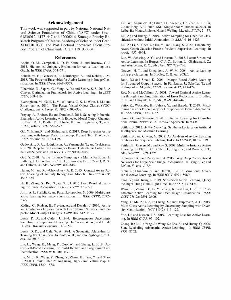
Figure 7: Visualization of object predictions of the two ad-versarial classifiers. The first row shows the original images,the second and the third rows show the predictions of clas-sifier 1 and classifier 2 respectively. Redder colors indicatehigher scores. (Best viewed in color with zoom)

Object Detection

Following the settings in LL4AL (Yoo and Kweon 2019), weapply ADS to object detection using the SSD detector (Liuet al. 2016). We add two fully convolutional layers as the ad-versarial classifiers, which are 3 × 3 kernels with the strideof 1 and the padding of 1. For each image, all the featurevectors generated by the detector are fed to the ADS mod-ule for entropy calculation. For multiple feature vectors, thevector of the top-1000 largest entropy is used as the metricto determine whether the image is informative or not.

The experiments are conducted on PASCAL VOC 2007and 2012 (Everingham et al. 2010), where 1000 samples areselected from the training set as the initial labeled set. Ineach iteration, 1000 samples are selected and added to thelabeled set. The agreement-discrepancy module is trainedfor 30 epochs, while the labeled set training module for 150epochs. The agreement-discrepancy module only works forthe positive images which contain at least one object. Asshown in Fig. 6, ADS outperforms the state-of-the-arts, val-idating its effectiveness for object detection.

In Fig. 7, we visualize the predictions (classificationscores) of the two adversarial classifiers with score thresh-old 0.3 after the NMS step with IoU threshold 0.5. It canbe seen that ADS produces informative predictions with dis-crepant scores. The images containing larger discrepancy areselected for data annotation.

ConclusionWe proposed the Agreement-Discrepancy-Selection (ADS)approach for active learning and unify the distribution align-ment with sample selection by introducing adversarial clas-sifiers. By operating the classifiers’ prediction agreementand discrepancy, ADS quantified the distribution overlapand bias without directly predicting the uncertainty or di-versity of samples. With well-designed calibration weights,ADS further differentiated the alignment and discrepancy ofunlabeled samples, which facilitates informative sample se-lection. Experiments on image classification and object de-tection benchmarks demonstrate the task-agnostic advantageof ADS. The ADS approach provides a fresh insight to theclassical active learning problem.

AcknowledgementThis work was supported in part by National National Nat-ural Science Foundation of China (NSFC) under Grant61836012, 61771447 and 62006216, Strategic Priority Re-search Program of Chinese Academy of Science under GrantXDA27010303, and Post Doctoral Innovative Talent Sup-port Program of China under Grant 119103S304.

ReferencesAodha, O. M.; Campbell, N. D. F.; Kautz, J.; and Brostow, G. J.2014. Hierarchical Subquery Evaluation for Active Learning on aGraph. In IEEE CVPR, 564–571.

Beluch, W. H.; Genewein, T.; Nurnberger, A.; and Kohler, J. M.2018. The Power of Ensembles for Active Learning in Image Clas-sification. In IEEE CVPR, 9368–9377.

Elhamifar, E.; Sapiro, G.; Yang, A. Y.; and Sastry, S. S. 2013. AConvex Optimization Framework for Active Learning. In IEEEICCV, 209–216.

Everingham, M.; Gool, L. V.; Williams, C. K. I.; Winn, J. M.; andZisserman, A. 2010. The Pascal Visual Object Classes (VOC)Challenge. Int. J. Comp. Vis. 88(2): 303–338.

Freytag, A.; Rodner, E.; and Denzler, J. 2014. Selecting InfluentialExamples: Active Learning with Expected Model Output Changes.In Fleet, D. J.; Pajdla, T.; Schiele, B.; and Tuytelaars, T., eds.,ECCV, volume 8692, 562–577.

Gal, Y.; Islam, R.; and Ghahramani, Z. 2017. Deep Bayesian ActiveLearning with Image Data. In Precup, D.; and Teh, Y. W., eds.,ICML, volume 70, 1183–1192.

Gudovskiy, D. A.; Hodgkinson, A.; Yamaguchi, T.; and Tsukizawa,S. 2020. Deep Active Learning for Biased Datasets via Fisher Ker-nel Self-Supervision. In IEEE CVPR, 9038–9046.

Guo, Y. 2010. Active Instance Sampling via Matrix Partition. InLafferty, J. D.; Williams, C. K. I.; Shawe-Taylor, J.; Zemel, R. S.;and Culotta, A., eds., NeurIPS, 802–810.

Hasan, M.; and Roy-Chowdhury, A. K. 2015. Context Aware Ac-tive Learning of Activity Recognition Models. In IEEE ICCV,4543–4551.

He, K.; Zhang, X.; Ren, S.; and Sun, J. 2016. Deep Residual Learn-ing for Image Recognition. In IEEE CVPR, 770–778.

Joshi, A. J.; Porikli, F.; and Papanikolopoulos, N. 2009. Multi-classactive learning for image classification. In IEEE CVPR, 2372–2379.

Kading, C.; Rodner, E.; Freytag, A.; and Denzler, J. 2016. Activeand Continuous Exploration with Deep Neural Networks and Ex-pected Model Output Changes. CoRR abs/1612.06129.

Lewis, D. D.; and Catlett, J. 1994. Heterogeneous UncertaintySampling for Supervised Learning. In Cohen, W. W.; and Hirsh,H., eds., Machine Learning, 148–156.

Lewis, D. D.; and Gale, W. A. 1994. A Sequential Algorithm forTraining Text Classifiers. In Croft, W. B.; and van Rijsbergen, C. J.,eds., SIGIR, 3–12.

Lin, L.; Wang, K.; Meng, D.; Zuo, W.; and Zhang, L. 2018. Ac-tive Self-Paced Learning for Cost-Effective and Progressive FaceIdentification. IEEE PAMI 40(1): 7–19.

Lin, M.; Ji, R.; Wang, Y.; Zhang, Y.; Zhang, B.; Tian, Y.; and Shao,L. 2020. HRank: Filter Pruning using High-Rank Feature Map. InIEEE CVPR, 1529–1538.

Liu, W.; Anguelov, D.; Erhan, D.; Szegedy, C.; Reed, S. E.; Fu,C.; and Berg, A. C. 2016. SSD: Single Shot MultiBox Detector. InLeibe, B.; Matas, J.; Sebe, N.; and Welling, M., eds., ECCV, 21–37.

Liu, Z.; and Huang, S. 2019. Active Sampling for Open-Set Clas-sification without Initial Annotation. In AAAI, 4416–4423.

Liu, Z.; Li, S.; Chen, S.; Hu, Y.; and Huang, S. 2020. UncertaintyAware Graph Gaussian Process for Semi-Supervised Learning. InAAAI, 4957–4964.

Luo, W.; Schwing, A. G.; and Urtasun, R. 2013. Latent StructuredActive Learning. In Burges, C. J. C.; Bottou, L.; Ghahramani, Z.;and Weinberger, K. Q., eds., NeurIPS, 728–736.

Nguyen, H. T.; and Smeulders, A. W. M. 2004. Active learningusing pre-clustering. In Brodley, C. E., ed., ICML.

Roth, D.; and Small, K. 2006. Margin-Based Active Learningfor Structured Output Spaces. In Furnkranz, J.; Scheffer, T.; andSpiliopoulou, M., eds., ECML, volume 4212, 413–424.

Roy, N.; and McCallum, A. 2001. Toward Optimal Active Learn-ing through Sampling Estimation of Error Reduction. In Brodley,C. E.; and Danyluk, A. P., eds., ICML, 441–448.

Saito, K.; Watanabe, K.; Ushiku, Y.; and Harada, T. 2018. Maxi-mum Classifier Discrepancy for Unsupervised Domain Adaptation.In IEEE CVPR, 3723–3732.

Sener, O.; and Savarese, S. 2018. Active Learning for Convolu-tional Neural Networks: A Core-Set Approach. In ICLR.

Settles, B. 2012. Active Learning. Synthesis Lectures on ArtificialIntelligence and Machine Learning.

Settles, B.; and Craven, M. 2008. An Analysis of Active LearningStrategies for Sequence Labeling Tasks. In EMNLP, 1070–1079.

Settles, B.; Craven, M.; and Ray, S. 2007. Multiple-Instance ActiveLearning. In Platt, J. C.; Koller, D.; Singer, Y.; and Roweis, S. T.,eds., NeurIPS, 1289–1296.

Simonyan, K.; and Zisserman, A. 2015. Very Deep ConvolutionalNetworks for Large-Scale Image Recognition. In Bengio, Y.; andLeCun, Y., eds., ICLR.

Sinha, S.; Ebrahimi, S.; and Darrell, T. 2019. Variational Adver-sarial Active Learning. In IEEE ICCV, 5971–5980.

Tang, Y.; and Huang, S. 2019. Self-Paced Active Learning: Querythe Right Thing at the Right Time. In AAAI, 5117–5124.

Wang, K.; Zhang, D.; Li, Y.; Zhang, R.; and Lin, L. 2017. Cost-Effective Active Learning for Deep Image Classification. IEEECSVT 27(12): 2591–2600.

Yang, Y.; Ma, Z.; Nie, F.; Chang, X.; and Hauptmann, A. G. 2015.Multi-Class Active Learning by Uncertainty Sampling with Diver-sity Maximization. IJCV 113(2): 113–127.

Yoo, D.; and Kweon, I. S. 2019. Learning Loss for Active Learn-ing. In IEEE CVPR, 93–102.

Zhang, B.; Li, L.; Yang, S.; Wang, S.; Zha, Z.; and Huang, Q. 2020.State-Relabeling Adversarial Active Learning. In IEEE CVPR,8753–8762.