WORKING PAPER SERIES

Aging, Myopia, and the Pay-As-You-Go Public Pension

Systems of the G7: A Bright Future?

Rowena A. Pecchenino and

Patricia S. Pollard

Working Paper 2000-015C http://research.stlouisfed.org/wp/2000/2000-015.pdf

July 2000 Revised October 2003

FEDERAL RESERVE BANK OF ST. LOUIS Research Division 411 Locust Street

St. Louis, MO 63102

______________________________________________________________________________________

The views expressed are those of the individual authors and do not necessarily reflect official positions of the Federal Reserve Bank of St. Louis, the Federal Reserve System, or the Board of Governors.

Federal Reserve Bank of St. Louis Working Papers are preliminary materials circulated to stimulate discussion and critical comment. References in publications to Federal Reserve Bank of St. Louis Working Papers (other than an acknowledgment that the writer has had access to unpublished material) should be cleared with the author or authors.

Photo courtesy of The Gateway Arch, St. Louis, MO. www.gatewayarch.com

Aging, Myopia, and the Pay-As-You-Go Public Pension Systems of the G7:

A Bright Future?

Rowena A. Pecchenino* and Patricia S. Pollard**

*Department of Economics Michigan State University

East Lansing, MI 48824-1038 517-353-6621

rowenap@msu.edu

**Federal Reserve Bank of St. Louis 411 Locust Street

St. Louis, MO 63102 314-444-8557

314-444-8731 (fax) pollard@stls.frb.org

July 2001 Revised September 2003

JEL Codes: D9, E6, H2, I2 Keywords: myopia, public pension, endogenous growth The public pension systems of the G7 countries were established in an era when the number of contributors far outweighed the number of beneficiaries. Now, for each beneficiary there are fewer contributors, and this trend is projected to accelerate. To evaluate the prospects for these economies we develop an overlapping generations model where growth is endogenously fueled by investments in physical and human capital. We analyze individuals’ behavior when their expectations over their length of life are rational or myopic and examine whether policies exist that can offset the effects of aging, should they be adverse. We find that while perfectly anticipated aging is welfare improving and does not threaten the solvency of public pension systems, myopia worsens welfare, puts pension systems at risk, and cannot be easily remedied by public policy. The views expressed in this paper are solely those of the authors and do not necessarily reflect the views of the Federal Reserve Bank of St. Louis, or of the Federal Reserve System.

"Population aging is the single most consistent pressure on federal income security

spending, as public pension spending continues its relentless upward climb."

Douglas Young, former Canadian Minister of Human Resources Development

I. Introduction

The public pension systems of the G7 countries were established in an era when the number of

contributors to the pay-as-you-go schemes far outweighed the number of beneficiaries. Over the post-

World War II period the systems have matured and the populations of the G7 countries have aged as

longevity has risen and birth rates have fallen. Now, for each beneficiary there are fewer contributors,

and this downward trend is projected to accelerate. To maintain benefit levels, tax rates and/or

productivity growth will have to rise. Evaluating the future of the systems, individual contributors

express grave doubts that they will receive as they did give (Saito, 1998).

To evaluate the prospects for these economies we develop an overlapping generations model in

which individuals face uncertainty over their longevity, growth is endogenously fueled by individuals’

investments in physical capital, and individual and government investment in human capital. All retirees

receive public pension benefits, funded in a pay-as-you-go manner. We analyze individuals’ behavior

and social welfare when expectations over length of life are rational or adaptive (myopic). Using

simulations of our model in which parameter values are drawn from the individual economies of the G7,

we examine for each of the economies and for each of the expectations assumptions whether policies exist

that can offset any adverse effects of aging. Further, we examine how policies aimed at a specific target

group, e.g. the elderly or the young, affect current and future welfare of the economy as a whole.

Our model is similar in construct to Docquier and Michel (1999) and Kaganovich and Zilcha

(1999), which also examine the effects of the public funding of pensions and education on economic

growth.1 We, however, as in Glomm and Kaganovich (2002), take the constraints of the public pension

system (benefits are determined as a replacement rate on wages, so benefits determine taxes) explicitly

1

into account in our analysis. Thus we assume that the government, effectively, faces two budget

constraints, a public pension constraint and an education constraint, rather than a unified constraint with

the explicit tradeoff assumed (more for public pensions implies less for education). Kaganovich and

Zilcha focus on the trade-off between education and public pension spending absent an aging population.

Docquier and Michel incorporate population growth to model a transitory demographic shock, whereas

we model a demographic transition. Our model differs from these and other studies, such as Auerbach et

al. (1989) and Hviding and Mérette (1998), in that we incorporate uncertainty regarding length of life;

thus allowing us to determine the importance of expectations regarding longevity.

Our model differs from previous studies of myopia and public pensions in that we are not

attempting to determine the optimal structure of the public pensions given myopia, as in Feldstein (1985)

and Hu (1996). Our work takes the current systems in the G7 countries as given, examines the effects of

myopia on economic growth and welfare, and looks for policies to ameliorate those effects, if adverse.

Our findings suggest that perfectly anticipated population aging may be beneficial to the

economy as a whole and does not pose a threat to the solvency of the public pension system. Greater

longevity induces higher rates of saving for retirement, whereas declining population growth increases

human capital expenditures per child. These effects offset the negative effects of the higher tax rate that

is necessary to maintain a given stream of public pension benefits. As a result the growth rate of output

per worker rises, and with it, welfare.2 Nonetheless, in nearly every country, aggregate saving declines

resulting in a reduction in the growth rate of aggregate output.3

When agents are myopic, both social welfare and growth are adversely affected because taxes rise

but the positive longevity effect on saving is absent. Any policy targeted at retirees, e.g., to maintain their

standard of living over their individually unanticipated longer lives, will exacerbate the problem because

taxes to fund such a program will further reduce saving. Policies directed at the very young, such as

1 For a review of the literature relating to public pensions and education, see Kaganovich and Zilcha (1999). 2 In contrast, Turner et al. (1998) find that aging reduces the growth rate of GNP per capita. 3 Most studies of aging focus on aggregate saving and find that aging reduces the saving rate. See, for example, Auerbach et al. (1989), Hviding and Mérette (1998), Masson and Tryon (1990), and Roseveare et al. (1996).

2

higher expenditures on public education, may generate positive growth effects but will not benefit the

initial generation of retirees, as the effects are felt only with a lag. For such policies to offset the effects

of both myopia and aging, they must be put in place prior to the onset of aging. Thus, myopia, not aging

per se, is the biggest threat to public pension system viability.

II. The Model

The model developed below is an application of Pecchenino and Pollard (2002)4 and is similar to

that of Kaganovich and Zilcha (1999). There is an infinitely lived economy composed of finitely lived

individuals, firms, and a government. A new generation is born at the beginning of each period and lives

for at most three periods: youth, working age, and retirement. At each period t, N(t) identical agents of

generation t enter the workforce. The working age population grows at the rate n(t).

Consumers

At date t, agents in the first period of their lives, the young, neither consume nor produce. They

are endowed with one unit of time that they combine inelastically with resources provided by their

parents, e(t), and the government, eg(t), to develop their human capital, ht+1(t+1). Agents in the second

period of their lives, the workers, supply their effective labor, the product of their one unit of time and

their human capital developed in youth, inelastically to firms. In return, they receive wage income,

w(t)ht(t) from which they pay a pension tax, τ(t), and a school tax, ω(t). They also may receive bequests,

B(t), from their parents, which are tax free. Their disposable income is divided between funding their

children’s human capital development, e(t), their current consumption, ct(t), and saving, s(t), for their

consumption when retired, ct(t+1). Agents in the final period of their lives, the retirees, supply their

savings, s(t-1), inelastically to firms and consume their public pension benefits, T(t), and the return to

their savings, (1+ρ(t))s(t-1). With probability p(t-1) an agent who worked during period t-1 will live

throughout the retirement period, and with probability (1-p(t-1)) the agent will die at the onset of

3

retirement. Agents may form expectations of living into retirement rationally or adaptively (myopically).

Rational expectations means that working-age agents know their probability of dying at the onset of

retirement; they have perfect foresight. Adaptive expectations means that a working-age individual

assumes that his life expectancy is a convex combination of the actuarial forecast, p(t), the life expectancy

of his parents’ generation, p(t-1), and possibly the life expectancy of his grandparents’ generation, p(t-2).

Let be the member of generation t’s assessment of life expectancy. If an agent dies at the onset of )(ˆ tp

retirement, his saving is bequeathed to the members of generation t, )1())](1/())(1[()( −++= tstnttB ρ .

Personal saving in this model is the equivalent of the sum of the occupational “second pillar” and

the personal “third pillar” of retirement security. This is because, in the context of this model, a defined-

contribution occupational pension plan will earn the same return as private saving. Thus, as long as the

defined contribution is less than or equal to what agents would choose to save absent the program,

combining these two pillars has no affect on the behavior of the model.

For tractability, let the preferences of a representative worker at time t be represented by

.ln))1(1(ln)(ˆln 1 1)+(thtn + 1)+(tctp + (t)c = U tttt +++δ (1)

Parents get utility from consumption and from educating their children; the value of this education is

summarized by the child’s human capital. This utility is derived from an altruistic link between parent

and child rather than any personal return they may reap from their investment or other strategic motive

(see Cremer et al., 1992). This inter vivos bequest motive encompasses the lifetime bequest motive.

Since agents do not know when they will die, additional unintentional bequests may be forthcoming.

Parental and government investments are both essential for human capital formation. If a parent

invests e(t) and the government invests eg(t), then the child’s human capital will be

)t(g)t(t1t

21 )t(e)t(e)1t(h θθ=++ (2)

where the parameters θ1(t) and θ2(t) measure the elasticity of parental and government expenditures on

human capital, respectively. This modeling of educational attainment follows Hanushek’s (1992)

4 Derivations for this model follow those for Pecchenino and Pollard (2002). We direct the reader there for a more

4

achievement function. Parental, e(t), and governmental expenditures, eg(t), and the efficiency of those

expenditures, θ1(t) and θ2(t), matter for human capital development. The utility a parent receives from his

dependent children’s human capital is )1(ln))1(1( 1 +++ + thtn tδ ; δ is the discount factor.

The representative agent takes as given his human capital, wages, return on saving, the pension

and school tax rates, public pension benefits, bequests, and government expenditures on education. The

agent then chooses saving and education expenditures to maximize lifetime utility as given by equation

(1) subject to (2) and the following budget constraints

)())1(1()())1(1()())()(1)(()()( tBtptetntsttthtwtc tt −−+++−−−−= ωτ (3)

)+T(t + ))s(t)+(t+(1 = )+(tct 111 ρ (4)

where constraint (3) encompasses the assumption that bequests are allocated equally across all members

of a generation so that the bequest-dependent wealth distribution is uniform, as in Hubbard and Judd

(1987). This assumption allows us to conduct a representative agent analysis, and restricts uncertainty to

the timing of death alone.

The first-order conditions for this problem, with respect to s(t) and e(t), respectively, are

0)1(

))1(1)((ˆ)(

1=

+++

+−tc

ttptc tt

ρ (5)

0)()(

1 1 =+−tetct

δθ . (6)

Firms

The firms are perfectly competitive profit maximizers that produce output using the production function

Y(t) = , α ∈ (0, 1). K(t) is the capital stock at t, which depreciates fully in the αα −1)()()( tHtKtA

production process. H(t) is the effective labor input at t, H(t) = N(t)ht(t), where N(t) is labor hours. A(t)>

0 is a productivity scalar. The production function can be written in intensive form

(7) αα )t(k)t(h)t(A)t(y 1t

−=

detailed discussion of the underlying assumptions, etc.

5

where y(t) is output per worker and k(t) is the capital labor ratio.

Firms take the wage, w(t), and rental rate, R(t), as given. They hire effective labor and capital up

to the point where their marginal products equal their factor prices:

w(t)= )k(t)t(h)t()A-(1 tααα − (8)

. (9) R(t) = )k(t)t(h)A(t 11t

−− ααα

The Government

The government administers the public pension program and funds education. It levies

proportional income taxes, τ(t) and ω(t), on the workers to finance pension and education expenditures,

respectively. Public pension benefits are specified as a replacement rate on the wages of current workers.

Thus, )()()1()( thtwttT t−= ξ where T(t) are the transfers to the retired at date t and ξ(t-1) is the

replacement rate for retirees in period t, which is set in period t-1. The tax rate, τ(t), adjusts to ensure that

public pension benefits equal tax revenues

)()()()()()(1

)1()1()()(1)1( thtwtthtw

tnttptT

tntp

tt τξ=

+−−

=+

− . (10)

Solving equation (10) for τ(t) yields

)(1)1()1()(

tnttpt

+−−

=ξτ (11)

Similarly, total government spending on education must equal total school tax revenues

)()1(1

)( tw(t)htnt = (t)e t

g

++ω . (12)

The Goods Market

The goods market clears when the demand for goods equals the supply of goods:

)()()()()())(1()())(1()()()(1)1()( 1 tktRthtwtetntetntstc

tntptc t

gtt +=+++++

+−

+ − (13)

6

Substituting equations (3), (4), (8), (9), (11), and (12) into (13), and making use of the fact that by

arbitrage the return on capital must equal the return on saving,

(t) + 1 = R(t) ρ (14)

yields

s(t-1)=(1+n(t))k(t). (15)

III. Equilibrium

Definition: A competitive equilibrium for this economy is a sequence of prices and taxes

, a sequence of allocations and a sequence of human and

physical capital stocks, , , given, such that given agents’ expectations

regarding longevity, and given these prices, allocations, and capital stocks, agents’ utility is maximized,

firms’ profits are maximized, the government budget constraints are satisfied, and markets clear.

∞0=t(t)} (t), (t), {w(t), ωτρ ∞

=+ 0)}1(),({ ttt tctc

∞=0)}(),({ tt tkth )0(k 0)0(0 >h

Substituting equations (2)-(4), (8), (9), (11), (12), (14) and (15) into the first order conditions

given by equations (5) and (6) results in the following set of difference equations in k(t+1), e(t) and

predetermined variables.

01 )1+k(t)t()1( + )1t(n1

)t(p =−⎟⎠⎞

⎜⎝⎛ −

++Λ

αξα

(16)

and

01)t(e

1 =−Λ

δθ (17)

where

)]1t(ke(t))][t(n1[)k(t)1(te)1e(t)]1t(p1[+)(1)t()t(n1

)1t()1t(p1)t(A )-(1)1t(g)1)(1t( 21 +++−−−⎥⎥⎦

⎤

⎢⎢⎣

⎡−−−⎟⎟

⎠

⎞⎜⎜⎝

⎛−

+−−

−= −−− ααθαθααωξ

Λ

7

IV. The Analytics of Growth

The following results are for the balanced growth specification of the model. Similar results hold

for the steady-state model specification. The proofs are in the appendix.

Proposition 1: Assume all parameter values are time independent, so x(t) = x for all t and for all

parameters x. Then, economies with higher school taxes, ω, will have higher growth rates if ωω >ˆ ,

where ( )[ ].)p1()1()n1/(p1ˆ 2 ααξθω −+−+−=

The school tax rate, ω, represents the marginal cost of public education while the marginal benefit

to the taxpayer, ,ω is the marginal increase in income during one’s working years, discounted by the

marginal efficiency of the government’s educational input, θ2. If ωω >ˆ , agents receive a positive income

effect from an increase in the school tax rate, leading to increases in saving and investment in one’s

children’s human capital. If ωω <ˆ , both saving and human capital investment fall. Thus, as Hanushek

and Kim (1996) suggest, the economic benefits from education are higher the higher is the quality of the

education, here measured by θ2.

If the economy is not on a balanced growth path then increases in the school tax from a

suboptimal level toward a growth-maximizing level can have growth-increasing effects if the positive

human capital effect tomorrow exceeds the negative physical capital effect today.

The following two propositions examine how economic growth is affected by changes in the two

demographic parameters: expected longevity, , and the population growth rate, n. A rise in affects p p

growth through three channels. The expectation of a longer life increases saving for retirement (longevity

effect). A longer lifespan reduces bequests (bequest effect) and a longer lifespan increases the tax rate

required to fund public pension benefits (public pension effect), as shown in equation (11). The first

effect raises the economic growth rate while the latter two lower it.

A decrease in n also has bequest and public pension effects. A decline in n results in a rise in

bequests received by each worker but raises the pension tax rate, a shown in equation (11). A fall in the

8

population growth rate raises educational expenditures per child (the education effect) and raises saving

per worker (family size effect). All but the public pension effect raise the growth rate of the economy.

Proposition 2: Economies in which expected longevity, , is higher have higher growth rates if p

the longevity effect dominates the bequest and public pension tax effects.

If agents expect to live longer, then, all else equal (including the age of retirement), they consume

a higher proportion of their saving and leave less to their children. This negative bequest effect reduces

expected income for working-age agents, reducing saving. Since pension taxes increase as longevity

rises, income while working falls, compounding the negative bequest effect. The tax effect would be

greater if labor supply were elastic, as some agents would choose to work less in response to the higher

taxes. On the other hand workers expecting a longer lifespan increase their saving. If the longevity effect

is dominant, physical capital accumulation and the equilibrium growth rate will rise.

When the increase in longevity is unexpected only the negative bequest and public pension

effects remain. For example, suppose at date t agents plan for the future expecting an unchanged

demographic structure. If they live longer than expected, their saving will be inadequate to fund their

longer life at the anticipated level of consumption. That is, their consumption will be lower than it would

have been had they anticipated a higher probability of living into old age. Further, the bequests they leave

to their children will be smaller, leaving them with less income. Their children’s income is further

reduced by the rise in public pension taxes as a result of the increased longevity. Even one generation of

unexpectedly long-lived agents can have permanent effects on the height of the growth path, if not on the

long-run equilibrium rate of growth.

Proposition 3: Economies with lower population growth rates, n, have higher growth rates if the

sum of the education and family size effects is positive and exceeds the public pension effect.

With fewer children, education expenditures per child are higher. In addition, the bequest each of

these children receives is higher. There are, however, two competing income effects. The family size

effect is the standard Solow growth model effect of a lower population growth rate: higher per capita

saving. This positive effect is countered by a negative income effect, the public pension effect. Public

9

pension taxes are now higher to compensate for the smaller pool of taxpayers relative to retirees. If the

education, bequest, and family size effects exceed the public pension effect, then economies with lower

population growth rates will have higher equilibrium growth rates. If the tax effect dominates, a reduced

population growth rate may lead to reductions in economic growth and social welfare, even without the

added complication of longer lived elderly.

V. Simulations: System Sustainability and Social Welfare

In this section we examine the effects of demographic changes, both anticipated and

unanticipated, on growth and economic welfare. Social welfare in period t is

).(ln)]1(1[)(ln))](1/()1([)(ln)( 11 thtntctntptctW ttt +− ++++−+= δν (18)

Each generation’s consumption at time t is normalized by the size of the working age generation

at t, N(t). The weight given to the young, δ, is the same as the weight parents place on educating their

children. We assume that ν > 1; the weight given to the elderly is in excess of their population weight.

This allows for the initial optimality of a public pension program in an economy that is dynamically

efficient.5 That ν exceeds unity implies that society as a whole puts greater value on the living standards

of the elderly than on the living standards of the young or the middle-aged. This social valuation result

from the voting habits and political activity of the elderly. That the old have greater influence than their

population size would suggest is explored by Mulligan and Sala-i-Martin (1999). Or, it could be a

reflection of a negative external effect on the welfare of the middle aged and young of low living

standards of the elderly. Thus, while the young individually cannot affect this, society as a whole can.

All these provide a rationale for a public pension system in a dynamically efficient economy.

We begin by calibrating the model to match the recent growth experiences of each of the G7

economies. Each period is a generation, set equal to 25 years. The weight given by parents to the human

5 A public pension system may also be optimal in an economy with generation specific shocks. Such a system would require the possibility of transfers from workers to retirees and vice versa (Rangel and Zeckhauser, 2000). Since existing systems do not allow for such transfers, we assume that social welfare considerations prevail.

10

capital development of their children, δ, is 0.98, for all countries, reflecting parental altruism. The

additional weight placed on the elderly’s consumption, ν, is 3.0 (our results do not depend on the value of

this parameter). This assures that the public pension system is initially optimal in all countries.6 There is

no obvious best estimate for θ2, the elasticity of governmental expenditures on education. We initially

assume θ2 =0.8, high efficiency of governmental expenditures, but also consider θ2=0.1, low efficiency of

governmental expenditures. For balanced growth θ1+θ2=1, so our choice of θ2 ties down the value of θ1.

The initial values for the country specific parameters in the model are given in Table 1.7 The

share of physical capital, α, for each country is from Bernanke and Gürkaynak (2001). The school tax

rate, ω, is the 1995 ratio of public expenditures on all levels of education to GDP (OECD, 2001), adjusted

for labor’s share in output. The replacement rate, ξ, is the average public pension benefit as a percent of

the average gross wage in 1995 (Chand and Jaeger, 1996). France, Germany, and Italy have the most

generous public pension systems with replacement rates above 50 percent. Japan and the United

Kingdom have the least generous systems with replacement rates below 20 percent.

The growth rate of the working-age population, n, is given by the growth rate of the population

aged 20 to 64 between 1970 and 1995.8 Canada had the largest percentage increase in the working-age

population while the United Kingdom had the smallest. The ratio of the population of retirees to workers

in 1995 multiplied by the gross growth rate of the working-age population, (1+n), gives the value for p.

Using these baseline parameter values and setting the growth rate of output per worker at its

1970-1995 average rate (Heston, Summers and Aten, 2002), allows us to determine the value of the

constant, A, in the production function. We then introduce population aging and re-simulate the model,

keeping all other parameters at their initial values.

6 Because saving, and hence economic growth, is higher in the absence of a pay-as-you-go public pension system, over time the optimality of such a system is eliminated unless the weight placed on the elderly is ever increasing. 7 The equations for growth are in the appendix. 8 Population data and projections for all countries are from the U.S. Bureau of the Census, International Database, Tables 004 and 094. Data are based on the July 17, 2003 update.

11

Aging in our model is the result of two demographic factors: a decline in n and an increase in p.

Specifically, we assume life expectancy rises beginning with the generation entering the workforce in

period j: p(j)>p(j-1) and continues for an additional period: p(j+1)>p(j). Population growth slows

beginning with the children of generation j: n(j+1)<n(j) and continues with the next generation:

n(j+2)<n(j+1). These changes result in a reduction in the size of the working age population relative to

the retired population. The parameters corresponding to this demographic transition, given in Table 2, are

based on the demographic projections for 2020 and 2045. By the second period, the population growth

rate is negative in all countries except Canada and the United States. To prevent a collapse of the

working age population in our model, we assume that the working age population remains constant

following the two period transition, as does longevity. As the population ages, the pension tax rate, τ,

rises to maintain the replacement rate as shown in equation (11).

Perfect Foresight

First, assume that agents have perfect foresight: they know the relevant value of p for their

generation: =p(t). The combined effect of increasing longevity and declining population growth

rates results in a rise in saving per worker and human capital investment per child. These in turn increase

output per worker as shown in Figure 1.

)(ˆ tp

Increasing p at t=j has a positive effect on saving in period j, a longevity effect. In addition,

generation j’s human capital expenditures per child rise as n(j+1) declines, a positive education effect.

Both effects boost output per worker in period j+1.

In period j+1 longevity continues to rise and the population growth rate continues to decline.

However, the positive longevity and education effects are now tempered by the negative bequest and

public pension effects of the rise in p(j) and the fall in n(j+1). The boost in the growth rate of output per

worker as a result of the change in demographics in the previous period, in combination with the

12

longevity and education effects, ensure a further rise in the growth rate of output per worker in period j+2

in all countries.

In period j+2 longevity remains unchanged. The population of children in this period is now the

same as the working age population, n(j+3)=0. For Canada and the United States this is a decline in the

population growth rate but for the other five countries the growth rate of the population rises, as n(j+2)

was negative. Thus, in the United States and Canada human capital expenditures per child continue to

rise, while in the other five countries the rise in n(j+3) has the opposite effect. In all countries the

negative bequest and public pension effects continue. In Canada the negative effects offset the education

effect and the per worker growth rate falls slightly. Only in the United States does the growth rate in

period j+3 rise.

In period j+3 there is a negative public pension effect in Canada and the United States as a result

of the decline in n(j+3), but a positive effect in the other five countries. Thus, the per worker growth rate

of output falls slightly in period j+4 in the former two countries and rises in the other five. At this point

the demographic transition is complete and the growth rate of output per worker is at its new, higher

equilibrium.

A declining population growth rate will reduce the growth rate of aggregate output unless it is

offset by a rise in the growth rate of output per worker. Only in Japan and the United Kingdom, is the rise

in output per worker sufficient enough to produce a rise in the long-run growth rate of aggregate output,

as illustrated in Figure 1. In these two countries, greater longevity, in combination with a low

replacement rate, ξ, causes a rapid rise in saving to fund retirement, driving the rise in the growth rate of

aggregate output.

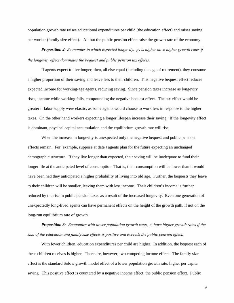
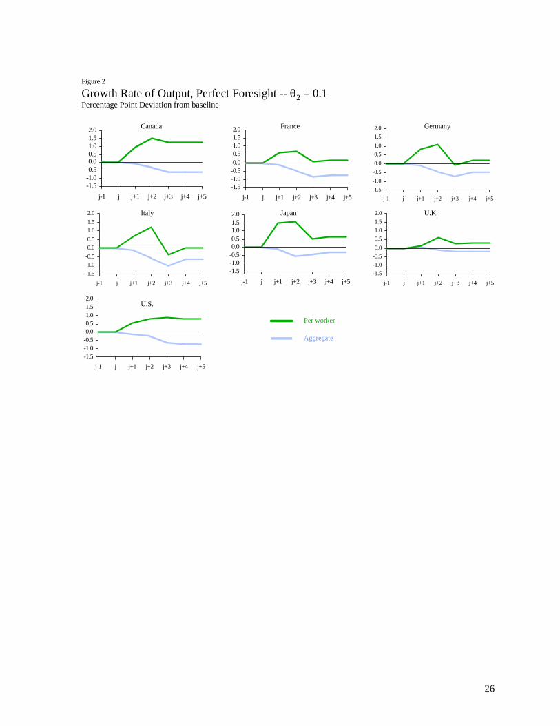
The importance of the efficiency of government expenditures on education is illustrated by Figure

2, which shows the results of simulating the model assuming that θ2 =0.1 for all countries. Lowering the

estimate of θ2 results in a smaller rise in the growth rate of output per worker. In Germany and Italy

13

output per worker falls relative to the baseline during part of the transition. The lower θ2 produces a

decline in aggregate output in all countries.

The demographic changes affect welfare through their effects on the weight given to each

generation and on consumption. The increase in longevity raises the weight placed on the consumption

of the retired generation and has a positive effect on welfare, as can be seen in equation (18). The

decline in the growth rate of the working age population, first reduces the weight placed on human capital

expenditures on children (a negative effect on welfare); eventually it also increases the weight placed on

retirees, thus having an ambiguous effect on welfare. The positive effect of aging on the growth rate of

output per worker increases consumption and has a positive effect on welfare. In the long run the positive

effects dominate and welfare rises regardless of the choice of θ2, as shown in Figure 3.

In all countries, except the United Kingdom, the initial (period j) negative effect of an increase in

aging on welfare primarily results from the decrease in the population growth rate n(j+1). Specifically,

the middle-aged increase their consumption as the lower population growth rate reduces parental

expenditures on children, although expenditures per child rise. The human capital of each child, hj+1(j),

rises, but the weight given to this generation in the welfare function falls as n(j+1) decreases. The

increase in consumption by the middle-aged is not large enough to offset this negative effect, and welfare

in period t=j falls. Over time, the increase in the growth rate of output per worker, resulting from

increased physical and human capital per worker, raises consumption and welfare for all generations.

The decline in n(j+1) is smallest in the United Kingdom,. In this country the effect of the rise in

p(j) predominates. The low replacement rate induces a sharp rise in saving given a rise in expected

longevity. In period j, consumption of the working age population declines as do parental expenditures

per child. Human capital per child, rises as an increase in government expenditures per child offsets the

decline in parental expenditures. Nevertheless, the decline in the weight given to the young in the welfare

function and the decline in the consumption of workers result in a drop in welfare.

14

Perfectly anticipated aging raises output per worker and the welfare of future generations. Yet,

an aging population results in substantial increases in public pension expenditures. Table 3 shows the

share of pension expenditures in output prior to and following the demographic transition. These

increases are similar to those estimated by Chand and Jaeger (1996) and Roseveare et al. (1996).

In our model the systems remain economically viable, that is, contributions cover expenditures.

This result may be affected by our assumption that labor supply is inelastic. If labor force participation

rates are sensitive to the tax rate, τ, then as the economy ages labor force participation rates fall as

workers move, for example, into the informal sector. Under these circumstances the systems in some

countries may become insolvent.

Adaptive (Myopic) Expectations

We next conduct a number of simulations under alternative assumptions on individuals’

expectations of their longevity and compare these with the perfect foresight results. To do so we assume

that a working-age agent assumes his life expectancy is a convex combination of the actuarial forecast,

p(t), the life expectancy of his parents’ generation, p(t-1), and, possibly, the life expectancy of his

grandparents’ generation, p(t-2).9 Thus, define

)3()1()()(ˆ 321 −+−+= tptptptp λλλ , where 1,, 321 ≤λλλ and 213 1 λλλ −−= . (19)

We present results for three possible combinations of the λs. The first specification is 5.021 == λλ :

individuals place equal weight on the actuarial forecast and the experience of their parents’ generation in

assessing their own life expectancy. The second specification is λ2=1. Individuals assess their probability

of living into retirement as equivalent to that of their parents’ generation. The third specification is λ3=1.

Individuals assess their probability of living into retirement as equivalent to that of their grandparents’

generation. In all specifications, upon reaching retirement age, the true p is revealed.

15

Myopia is harmful to economic growth, either on a per worker or aggregate basis. This is because

as longevity increases and this increase is not taken into account, agents do not save adequately for their,

unanticipated, longer lives.10 In the terminology of Proposition 2, the longevity effect disappears and

only the negative income and bequest effects remain.11 Because, in our model, p stabilizes after two

periods, a myopic economy’s growth rate converges to the perfect foresight long-run equilibrium value.

Welfare in the initial period, t=j, is higher under myopia than under perfect foresight, as shown in

Figure 4. The failure of workers to recognize an increase in longevity results in a shift in the allocation of

income away from saving and toward current expenditures, relative to perfect foresight. Parental

expenditures on children, as well as own consumption, rise. Since the initial generation of retirees are

unaffected, welfare unambiguously rises. Although the rise in education expenditures in period j has a

beneficial effect on output in the next period, it cannot offset the negative effect of the decline in saving.

The fall in output in j+1 and lower bequests relative to perfect foresight results in a decline in the working

age population’s own consumption expenditures, and their expenditures on education. Also, the retired

generation now reduces its consumption relative to the baseline due to the lack of adequate saving.

Welfare falls and continues to fall, as shown in Figure 4, until the demographic transition is fully

incorporated into individuals’ saving behavior. Thereafter, the difference between welfare under myopia

and perfect foresight narrows. The lower saving of the myopic generations leads to permanent decline in

welfare relative to perfect foresight. The greater the degree of myopia, the greater is the loss in welfare.

The extent to which myopia results in a reduction in welfare varies across countries. The greatest

reduction in welfare occurs in Germany and the smallest reduction in the United States.

Myopia is often given as a reason for the existence of public pension systems. Yet, Feldstein

(1985) showed that even if everyone in the economy is myopic, it still may be optimal to have no public

pension system. A similar result follows from our model. As Figure 5 shows, the long-run deviation of

9 This simple formulation incorporates both myopia and learning. 10 In our model, myopic individuals save for retirement, but their savings are inadequate given the increase in p. This is different from Feldstein (1985) and Hu (1996) in which myopic agents save nothing for retirement.

16

welfare under myopia from perfect foresight is greater with a public pension system than without one. In

addition, the short-run gain from myopia is higher in the absence of a public pension system. The

decrease in saving of the myopic generations relative to perfect foresight is higher in the presence of a

public pension system, while the increase in expenditures on one’s children is lower. Both effects

produce a lower growth rate, relative to perfect foresight, in an economy with a public pension system.

Japan is the country in or study that has already experienced substantial aging as a result of both a

sharp drop in the growth rate of the working age population and a rise in longevity. The growth rate of

aggregate output in Japan has fallen when comparing the periods 1950-1975 and 1975-2000. This decline

is consistent with either myopia or a low θ2. The growth rate of output per worker has also fallen in

Japan, in contrast to the prediction of our model. This difference could be explained by the effect on

growth of the rebuilding of the capital stock in the early postwar period.

School taxes

Faced with a myopic population, is there any means available to a government to effect higher

rates of saving? In our model, any forced saving plan, such as government-imposed mandatory pensions,

would have the effect of reducing an individual’s saving one-to-one (or more than one-to-one if the return

on government pensions exceeds the return on an individual’s own saving). Thus, to achieve an increase

in saving, government mandates would have to cause individuals to save in excess of their desired

amount. While this may make them better off in an ex post sense, it will not make them better off ex ante.

Evidence from the Australian superannuation funds (the privatized portion of its pension system)

provides support for the argument that governments are unable to force an increase in saving. In the first

five years after contributions to the system became mandatory, the $110 billion in accumulated assets

were mostly offset by borrowings (The Economist, 1998).

11 These results would be the same if agents had rational expectations, but the longevity projections upon which they

17

If the government increases the school tax prior to the onset of aging, individuals are forced to

save, in terms of their children’s human capital, but do not view paying the tax as forced saving. This tax

increase generates improvements in growth and social welfare.12 Figure 6 shows the effects of a 10

percent increase in the school tax rate on lifetime utility when myopia is most severe (λ3=1) and θ2=0.8.

The increase in welfare is lowest in Japan and highest in the United Kingdom. All other countries fall

within these ranges.

The value of θ2 is crucial to these results. When ω is increased, income of the working age

population initially falls and so agents reduce their saving and their expenditures on human capital. If the

efficiency of government expenditures on education is sufficiently high, then human capital and hence

output will rise. Moreover, this rise in human capital expenditures will more than offset the decline in

consumption of the working age population, resulting from the higher tax, and hence welfare will rise. As

Proposition 1 indicates, the lower is θ2 the lower is the optimal ω. In Canada, when θ2=1 the optimal

school tax rate is below the initial tax rate even prior to the demographic transition. Any increase in the

tax rate lowers welfare. In France and Italy welfare declines as the optimal school tax rate following the

demographic transition is below the new tax rate.

If agents view parental and governmental expenditures on education as perfect substitutes then

any attempt by the government to increase saving by raising the school tax rate will fail. Parents will

reduce their expenditures on their children in line with the rise in government education expenditures.

Trust Fund

Another way to handle myopia is through the use of a trust fund. The value of a trust fund in

period t is the difference between revenues and expenditures of the public pension system and the gross

return on any accumulated balances. The trust fund is equivalent to government savings:

based their savings decisions proved to be too low.

18

).1())](1/())(1[()()())](1/()1()1([)()()()( −++++−−−= tstntthtwtnttpthtwtts gtt

g ρξτ (21)

Now )())](1/()1()1([)( ttnttpt γξτ ++−−= , where )(tγ is the increase in the public pension tax rate to

support pre-funding of benefits. Equation (21) then can be rewritten as

)1())](1/())(1[()()()()( −+++= tstntthtwtts gt

g ργ . (22)

The capital stock at time t is now a combination of private saving, s(t-1), and public saving, sg(t-1). So

the goods market clearing equation (15) become s(t-1) = [1+n(t)]k(t) - sg(t-1).

The trust fund system can be set up in two ways. The first is to increase τ(t) (relative to the no

action policy) by setting γ(t)>0 in the periods in which myopia results in an underestimation of longevity

and lower τ in the next period(s) without changing ξ. For example, when λ2=1, τ(j) and τ(j+1) rise while

τ(j+2) and possibly τ(j+3) fall. The increase in τ reduces private saving both in terms of physical and

human capital, as well as consumption expenditures of the affected working-age generations. The decline

in private saving lowers consumption of the retired generation. All of these effects result in a reduction in

welfare for the duration of the policy. Nevertheless, the physical capital stock rises, because government

saving more than offsets the decline in private saving. As a result, welfare eventually rises once the trust

fund is exhausted.

The second method is to increase both τ(t) and ξ(t) for the myopic generations. When λ2=1, τ(j)

and τ(j+1) rise resulting in a two-generation trust fund. The replacement rates, ξ(j) and ξ(j+1), are

chosen so that the trust fund is exhausted in period j+1. The increase in the tax rate and the rise in the

replacement rate lower private saving by more than the increase in government saving. Total saving

declines and future generations are made worse off. Because of this negative effect on saving, pre-

funding the public pension system lowers welfare in all periods.

12 If the rational expectations longevity projections proved too low, no such policy would be possible.

19

VI. Conclusion

Over a period of several generations the proportion of retirees relative to workers is expected to

rise as the population growth rate declines and longevity rises. In the face of this demographic transition,

we assume that the government attempts to maintain the generosity of the public pension system by fixing

the replacement rate at its pre-aging rate. Given this policy, we examine the effects of aging on growth

and welfare under alternative assumptions on individuals’ expectations of longevity.

If individuals fully anticipate increased longevity, and hence increase saving for retirement, then

while aging generally reduces the growth rate of aggregate output, it need not reduce the growth rate of

output per worker. If individuals have perfect foresight and prefer a longer life to a shorter life, aging

does not reduce welfare in the long run. This prognosis is in stark contrast to Kotlikoff, Smetters and

Walliser (2001) and Gokhale and Kotlikoff (1999) who paint an unremittingly bleak portrait of the future

given the demographic transition. Their results and ours could be reconciled if they were to revise saving

behavior to account for myopia (under-saving given incorrect perception of longevity) and its correction

via learning (perfect foresight) or amelioration via induced human capital investment (school taxes).

If individuals are myopic, then during the demographic transition the economic growth falls

relative to perfect foresight. With myopic expectations the growth rate of the economy will, in the long

run, match the perfect foresight growth rate. Welfare receives an initial boost as myopic individuals

consume more and spend more on their children than the more frugal agents with perfect foresight. This

gain is short-lived. Welfare is lower in all subsequent periods as a result of the lower savings of the

myopic generations. These results are lower bounds since we have assumed that the supply of labor will

not fall when social security taxes rise. For small changes in taxes this assumption may be reasonable,

but this is not the case for the large changes in taxes forecast for many countries as they try to maintain

their public pension systems in the face of population aging.

Given a myopic population, few policies are available to the government to offset the adverse

growth and welfare effects. However, the government can raise the growth rate and welfare by inducing

saving through human capital development, i.e., raising the school tax rate. Such a policy, however, must

20

be in place prior to the onset of aging. In addition, the success of such a policy depends on the efficiency

of government expenditures on education. If government expenditures are not sufficiently productive

then raising school taxes will only exacerbate the effects of aging, lowering the output of the economy

(relative to no increase) and hence lowering welfare.

While myopia in our model results from agents’ failure to fully account for changing

demographics, the effects on saving are similar to models in which consumers fail to adjust to changes in

fiscal policies. Poterba (1988), for example, notes that while the U.S. public pension reforms enacted in

1983 reduced the present value of benefits for young workers, there is little evidence that these changes

have had any effect on saving behavior. These results indicate that myopia rather than aging is primarily

responsible for reducing growth and welfare when countries maintain their pay-as-you-go public pension

systems as the population ages.

21

References

Auerbach, A. J., L.J. Kotlikoff, R.P. Hagemann and G. Nicoletti (1989) “The Economic Dynamics of an Ageing Population: The Case of Four OECD Countries” OECD Economic Studies, Vol. 12 pp. 97-130.

Bernanke, B. S. and R. S. Gürkaynak (2001) “Is Growth Exogenous? Taking Mankiw, Romer, and Weil

Seriously” National Bureau of Economic Research Working Paper 8365.

Chand, S.K. and A. Jaeger (1996) “Aging Populations and Public Pension Schemes” IMF Occasional Paper 147.

Cremer, H., D. Kessler and P. Pestieau (1992) “Intergenerational Transfers within the Family” European

Economic Review, Vol. 36 pp.1-16. Docquier, M. and P. Michel (1999) “Education Subsidies, Social Security and Growth: The Implications

of a Demographic Shock” Scandinavian Journal of Economics, Vol. 101 pp. 425-40. The Economist (1998) “Retiring the State Pension” October 24-30. Feldstein, M. (1987) “The Optimal Level of Social Security Benefits” The Quarterly Journal of

Economics, Vol. 100 pp. 303-320. Glomm, G., and M. Kaganovich (2002) “Distributional Effects of Public Education in an Economy with

Public Pensions” unpublished manuscript, Indiana University. Gokhale, J., and L. Kotlikoff (1999) “Social Security’s Treatment of Postwar Americans: How Bad Can

It Get?” Federal Reserve Bank of Cleveland Working Paper 9912. Hanushek, E. A. (1992) “The Trade-Off Between Child Quantity and Quality” Journal of Political

Economy, Vol.100 pp. 84-117. Hanushek, E.A. and Kim, D. (1995), “Schooling, Labor Force Quality an Economic Growth” National

Bureau of Economic Research Working Paper 5399. Heston, A., R. Summers and B. Aten (2002) Penn World Table Version 6.1, Center for International

Comparisons at the University of Pennsylvania (CICUP). Hubbard, R.G. and K.L. Judd, (1987) “Social Security and Individual Welfare: Precautionary Saving,

Borrowing Constraints and the Payroll Tax” American Economic Review, Vol. 77 pp. 630-46. Hu, S. (1996) “Myopia and Social Security Financing” Public Finance Quarterly, Vol. 24 pp.319-48. Hviding, K. and M. Mérette (1998) “Macroeconomic Effects of Pension Reforms in the Context of

Ageing Populations: Overlapping Generations Model Simulations for Seven OECD Countries” OECD Ageing Working Papers, AWP 1.3.

Kaganovich, M. and I. Zilcha (1999) “Education, Social Security, and Growth” Journal of Public

Economics, Vol. 71 pp. 289-309.

22

Kotlikoff, L., K. Smetters, and J. Walliser (2001) “Finding a Way Out of America’s Demographic Dilemma” National Bureau of Economic Research Working Paper 8258.

Masson, P.R. and R.W. Tryon (1990) “Macroeconomic Effects of Projected Aging in Industrial

Countries” International Monetary Fund Staff Papers, Vol. 37 pp. 453-85. Mulligan, Casey and Xavier Sala-i-Martin (1999) “Social Security in Theory and Practice (II): Efficiency

Theories, Narrative Theories and Implications for Reform” National Bureau of Economic Research Working Paper 7119.

OECD, 2001, Education at a Glance: OECD Indicators, 2001 edition. Paris: OECD. Pecchenino, R. and P. Pollard, 2002, “Dependent Children and Aged Parents: Funding Education and

Social Security in an Aging Economy,” Journal of Macroeconomics 24, 145-69. Poterba, J. (1988) “Are Consumers Forward Looking? Evidence from Fiscal Experiments” American

Economic Review, Vol. 78 pp. 413-18. Rangel, A. and R. Zeckhauser (2000) “Can Market and Voting Institutions Generate Optimal

Intergenerational Risk Sharing?” in J. Campbell and M. Feldstein, eds., Risk Aspects of Investment-Based Social Security Reform. Chicago: University of Chicago Press.

Roseveare, D., W. Leibfritz, D. Fore and E. Wurzel (1996) “Ageing Populations, Pension Systems and

Government Budgets: Simulations for 20 OECD Countries” OECD Economic Department Working Papers No. 168.

Saito, J. (1998), “Pension System Reform Leaves Bitter Legacy” Asahi News Service, July 8. Turner, D., C. Giorno, A. De Serres, A. Vourc’h and P. Richardson (1998) “The Macroeconomic

Implications of Ageing in a Global Context” OECD Ageing Working Papers, AWP 1.2. U.S. Bureau of the Census, International Database, available at <<http://www.census.gov/ipc/www/>>.

23

Table 1 Baseline Parameter Values

Parameter Canada France Germany Italy Japan U.K. U.S. α 0.32 0.26 0.31 0.29 0.32 0.25 0.26 ξ 0.292 0.601 0.520 0.539 0.196 0.175 0.385 ω 0.091 0.080 0.065 0.063 0.053 0.065 0.067 n 0.581 0.241 0.177 0.164 0.260 0.114 0.450 p 0.312 0.318 0.289 0.309 0.290 0.298 0.313

Annual growth rate of output per worker 0.0105 0.0177 0.0129 0.0227 0.0287 0.0167 0.0152

Table 2 Demographic Change

Working-Age Population: Growth Rate Parameter Canada France Germany Italy Japan U.K. U.S.

n(j) 0.581 0.241 0.177 0.164 0.260 0.114 0.450 n(j+1) 0.235 0.040 -0.054 -0.040 -0.137 0.098 0.233

n(j+2) 0.012 -0.077 -0.192 -0.242 -0.242 -0.063 0.131 Longevity Parameter Canada France Germany Italy Japan U.K. U.S.

p(j-1) 0.312 0.318 0.289 0.309 0.290 0.298 0.313 p(j) 0.373 0.376 0.358 0.369 0.428 0.347 0.350

p(j+1) 0.452 0.459 0.465 0.509 0.519 0.430 0.431

Table 3 Expenditures on Public Pensions as a Percent of Output

Canada France Germany Italy Japan U.K. U.S. Pre-demographic transition 3.9 11.4 8.8 10.2 3.1 3.5 6.2

Post-demographic transition 9.0 20.4 16.8 19.5 6.9 5.6 12.3

24

-0.50.00.51.01.52.02.5

j-1 j j+1 j+2 j+3 j+4 j+5

-0.5

0.0

0.5

1.0

1.5

2.0

2.5

j-1 j j+1 j+2 j+3 j+4 j+5

-0.50.00.51.01.52.02.5

j-1 j j+1 j+2 j+3 j+4 j+5-0.5

0.0

0.5

1.0

1.5

2.0

2.5

j-1 j j+1 j+2 j+3 j+4 j+5

Figure 1

Growth Rate of Output, Perfect Foresight -- θ2 = 0.8Percentage Point Deviation from baseline

Canada France Germany

Japan U.K.

U.S.

Italy

-0.50.00.51.01.52.02.5

j-1 j j+1 j+2 j+3 j+4 j+5-0.5

0.0

0.5

1.0

1.5

2.0

2.5

j-1 j j+1 j+2 j+3 j+4 j+5

Aggregate

Per worker

-0.50.00.51.01.52.02.5

j-1 j j+1 j+2 j+3 j+4 j+5

25

-1.5-1.0-0.50.00.51.01.52.0

j-1 j j+1 j+2 j+3 j+4 j+5

-1.5-1.0-0.50.00.51.01.52.0

j-1 j j+1 j+2 j+3 j+4 j+5

-1.5-1.0-0.50.00.51.01.52.0

j-1 j j+1 j+2 j+3 j+4 j+5

-1.5-1.0-0.50.00.51.01.52.0

j-1 j j+1 j+2 j+3 j+4 j+5

-1.5-1.0-0.50.00.51.01.52.0

j-1 j j+1 j+2 j+3 j+4 j+5

Figure 2

Growth Rate of Output, Perfect Foresight -- θ2 = 0.1Percentage Point Deviation from baseline

Canada France Germany

Japan U.K.

U.S.

Italy

-1.5-1.0-0.50.00.51.01.52.0

j-1 j j+1 j+2 j+3 j+4 j+5

Aggregate

Per worker

-1.5-1.0-0.50.00.51.01.52.0

j-1 j j+1 j+2 j+3 j+4 j+5

26

-15

0

15

30

45

60

75

j-1 j j+1 j+2 j+3 j+4 j+5

Figure 3

Welfare -- Perfect ForesightDeviation from baseline

-15

0

15

30

45

60

75

j-1 j j+1 j+2 j+3 j+4 j+5

CanadaPercent

-15

0

15

30

45

60

75

j-1 j j+1 j+2 j+3 j+4 j+5

France

Percent

-15

0

15

30

45

60

75

j-1 j j+1 j+2 j+3 j+4 j+5

GermanyPercent Percent

JapanPercent

-15

0

15

30

45

60

75

j-1 j j+1 j+2 j+3 j+4 j+5

U.K.Percent

U.S.

-15

0

15

30

45

60

75

j-1 j j+1 j+2 j+3 j+4 j+5

Italy

Percent

22 = 0.1

22 = 0.8

-15

0

15

30

45

60

75

j-1 j j+1 j+2 j+3 j+4 j+5

27

-5

-4

-3

-2

-1

0

1

j-1 j j+1 j+2 j+3 j+4 j+5

Figure 4

Welfare Deviation from perfect foresight, θ2 =0.8

-5

-4

-3

-2

-1

0

1

j-1 j j+1 j+2 j+3 j+4 j+5

CanadaPercent

-5

-4

-3

-2

-1

0

1

j-1 j j+1 j+2 j+3 j+4 j+5

France

Percent

-5

-4

-3

-2

-1

0

1

j-1 j j+1 j+2 j+3 j+4 j+5

GermanyPercent Percent

-5

-4

-3

-2

-1

0

1

j-1 j j+1 j+2 j+3 j+4 j+5

JapanPercent

-5

-4

-3

-2

-1

0

1

j-1 j j+1 j+2 j+3 j+4 j+5

U.K.Percent

U.S.

-5

-4

-3

-2

-1

0

1

j-1 j j+1 j+2 j+3 j+4 j+5

Italy

Percent

λ1=λ2=0.5λ2=1λ3=1

28

-5

-4

-3

-2

-1

0

1

j-1 j j+1 j+2 j+3 j+4 j+5

-5

-4

-3

-2

-1

0

1

j-1 j j+1 j+2 j+3 j+4 j+5

Figure 5

WelfareDeviation from perfect foresight, λ3 =1, θ2 = 0.8

-5

-4

-3

-2

-1

0

1

j-1 j j+1 j+2 j+3 j+4 j+5

CanadaPercent

-5

-4

-3

-2

-1

0

1

j-1 j j+1 j+2 j+3 j+4 j+5

France

Percent

-5

-4

-3

-2

-1

0

1

j-1 j j+1 j+2 j+3 j+4 j+5

GermanyPercent Percent

-5

-4

-3

-2

-1

0

1

j-1 j j+1 j+2 j+3 j+4 j+5

JapanPercent

-5

-4

-3

-2

-1

0

1

j-1 j j+1 j+2 j+3 j+4 j+5

U.K.Percent

U.S.

Italy

Percent

With public pensionWithout public pension

Figure 6

Welfare With a 10% Increase in ωDeviation from original tax, λ3=1

0

1

2

3

4

5

6

j-1 j j+1 j+2 j+3 j+4 j+5

U.K.

Japan

Percent

29

Appendix

Balanced-growth solutions for capital and ouput

Combining equations (16) and (17)

)1()()( += tktte ϕ (A1)

where ⎥⎦⎤

⎢⎣⎡ −

+++=α

ξαδθϕ )()1()1(1

)(ˆ)(

)( 1 ttntpt

t .

Combining (A1) and (16) yields

[ ])1)(1()1)(1()1)(1(

1

1

121 )()1()1()()]1(1[)1()()(1

)1()1(1

)](1[)1(1)()()(

)1(

αθααθαθϕααωξ

ϕδθϕδθ

−−+−−−− −−⎥⎥⎦

⎤

⎢⎢⎣

⎡−−+−⎟⎟

⎠

⎞⎜⎜⎝

⎛−

+−−

−

×++++

=+

ttgt tktettAtpttnttp

ttnttt

tk

(A2)

From (8), (12), and (A2)

⎥⎥⎦

⎤

⎢⎢⎣

⎡−−+−⎟⎟

⎠

⎞⎜⎜⎝

⎛−

+−−

−++++

++

+−=

ααωξ

ϕδθϕδθ

ωα

)]1(1[)1()()(1

)1()1(1)](1)][1(1)[()(

))1(1)(()1()()1()(

1

1 tpttnttp

ttntttnt

tktte g (A3)

Lag (A3) and substitute it into (A2) to yield

(A4) )1))(()(( 21)()()1( αθθα −++=+ tttktZtk

where

⋅⎥⎦

⎤⎢⎣

⎡+

−−−

⎟⎟⎟⎟⎟⎟

⎠

⎞

⎜⎜⎜⎜⎜⎜

⎝

⎛

++++⎥⎥⎦

⎤

⎢⎢⎣

⎡−−+−⎟⎟

⎠

⎞⎜⎜⎝

⎛−

+−−

−

=−−

−−)1)(1(

)1)(1(

1

1 2

1

)(1)1)(1(

)1()()](1)][1(1)[()(

)]1(1[)1()()(1

)1()1(1)(

)(αθ

αθ αωϕ

ϕδθϕ

ααωξ

δθ tt

tnt

ttAttntt

tpttnttp

t

tZ

)1)(1(

1

1

2

)]2(1[)1()1()1(1

)2()2(1)1(

)]1(1)][(1)[1()1(

αθ

ααωξ

δθ

ϕδθϕ

−−

⎟⎟⎟⎟⎟⎟

⎠

⎞

⎜⎜⎜⎜⎜⎜

⎝

⎛

⎥⎥⎦

⎤

⎢⎢⎣

⎡−−+−⎟⎟

⎠

⎞⎜⎜⎝

⎛−−

−+−−

−−

−++−+−

t

tpttn

ttpt

ttntt .

30

When Z > 1 and θ1 + θ2 = 1, then k(t+1) > k(t) ∀ t.

Along a balanced growth path

)1()1()11)1(1

1

1 1222

1)1(

)1()1(1

1)1)(1(

αθαθαθ

ϕωα

ααωξ

ϕδθϕδθ −

−−−−−

⎟⎠

⎞⎜⎝

⎛+

−⎥⎦

⎤⎢⎣

⎡−+−⎟

⎠

⎞⎜⎝

⎛ −+

−⎟⎟⎠

⎞⎜⎜⎝

⎛+++

= An

pn

pn

Zα(θ

.

The growth rate of output per worker is

)1)(()1()1(

1

1^

2122

)t(Z)1t(

)t()1t(

)t()t(A

)1t(A

)t(k)t(h)t(A)1t(k)1t(h)1t(A

)t(y)1t(y)1t(y

αθθααθαθ

αα

αα

χχ

φφ −++

−−

−

−

⎟⎟⎠

⎞⎜⎜⎝

⎛−⎟⎟

⎠

⎞⎜⎜⎝

⎛−

+=

+++=

+=+

(A5)

where

⎥⎥⎦

⎤

⎢⎢⎣

⎡−−+−⎟⎟

⎠

⎞⎜⎜⎝

⎛−

+−−

−++++

++

−=

ααωξ

ϕδθϕδθ

ωαχ

)]1(1[)1()()(1

)1()1(1)](1)][1(1)[()(

)]1(1)[()()1()(

1

1 tpttnttp

ttntttnt

tt

Along a balanced growth path with θ1 + θ2 = 1, Zy = .

Proofs of Propositions

Proof of Proposition 1:

0)1()1)(

11(

)]1(1[)1( 22 >

⎪⎪⎭

⎪⎪⎬

⎫

⎪⎪⎩

⎪⎪⎨

⎧

−+−−+

−

−−−−=

∂∂

ααωξαθ

ωθ

αω p

np

ZZ

if

ωααξθ >−+−+

− ])1()1)(1

1[(2 pn

p.

31

Proof of Proposition 2:

0])1()1)(

11)[(1(

))1()1((

)1()1(1))1(1(

1))1(1(

1

2 >

⎪⎪⎭

⎪⎪⎬

⎫

⎪⎪⎩

⎪⎪⎨

⎧

⎥⎥⎥⎥

⎦

⎤

⎢⎢⎢⎢

⎣

⎡

−+−−+

−+

++−+

++⎟⎠

⎞⎜⎝

⎛ −++++

+−−−=

∂∂

ααωξ

ααξ

αξα

δθαθα

pn

pn

n

npnn

np

ZpZ

if the longevity effect exceeds the sum of the tax and bequest effects, that is if

⎥⎥⎥⎥

⎦

⎤

⎢⎢⎢⎢

⎣

⎡

−+−−+

−+

++−+

++⎟⎠

⎞⎜⎝

⎛ −+++

+−−>

])1()1)(1

1)[(1(

))1()1((

)1()1(

1))1(1(

1))1(1(

1

2ααω

ξααξ

αξα

δθαθα

pn

pn

n

npn

np

which is satisfied for p small. Proof of Proposition 3: For a decrease in n

0

)1()1(1

1)1(

)1(

)1()1(1)]1(1[

1)1(21)]1(1[

11)1(

11)1()1(

21

11

2

21

>

⎪⎪⎪⎪⎪⎪

⎭

⎪⎪⎪⎪⎪⎪

⎬

⎫

⎪⎪⎪⎪⎪⎪

⎩

⎪⎪⎪⎪⎪⎪

⎨

⎧

⎥⎥⎥⎥⎥

⎦

⎤

⎢⎢⎢⎢⎢

⎣

⎡

⎥⎦

⎤⎢⎣

⎡−+−⎟

⎠

⎞⎜⎝

⎛ −+

−+

−−

++⎟⎠

⎞⎜⎝

⎛ −++++

⎟⎠⎞

⎜⎝⎛ −

++++−−

−

⎟⎟⎠

⎞⎜⎜⎝

⎛⎟⎠⎞

⎜⎝⎛ −

+++

⎥⎦

⎤⎢⎣

⎡⎟⎠⎞

⎜⎝⎛ −

++−+−

−=∂∂

−

ααωξ

αξ

αξα

δθ

ξα

αδθδθαθ

ξα

α

ξα

αθθα

pn

pn

p

npnn

pn

nn

nn

ZnZ

if the sum of the education effect

⎟⎟⎠

⎞⎜⎜⎝

⎛⎟⎠⎞

⎜⎝⎛ −

+++

⎥⎦

⎤⎢⎣

⎡⎟⎠⎞

⎜⎝⎛ −

++−+−

−

ξα

α

ξα

αθθα

11)1(

11)1()1( 21

nn

nn

32

and the family size effect

⎥⎥⎥⎥

⎦

⎤

⎢⎢⎢⎢

⎣

⎡

++⎟⎠

⎞⎜⎝

⎛ −++++

⎟⎠⎞

⎜⎝⎛ −

++++−−

)1()1(

1)]1(1[

1)1(21)]1(1[

1

11

2npnn

pn

αξα

δθ

ξα

αδθδθαθ

is positive and exceeds the public pension tax effect

⎥⎥⎥⎥⎥

⎦

⎤

⎢⎢⎢⎢⎢

⎣

⎡

⎥⎦

⎤⎢⎣

⎡−+−⎟

⎠

⎞⎜⎝

⎛ −+

−+

−−−−

ααωξ

αξαθ

)1()1(1

1)1(

)1()]1(1[

22

pn

pn

p .

33