Aging: Modeling Time

Tom Emmons

This thing all things devours:Birds, beasts, trees, flowers;Gnaws iron, bites steel;Slays king, ruins town,And beats high mountain down

Outline

• Start Simple – only death

• Add properties– Birth– Age– Life Stages

• Some real life examples

Laws of Mortality

• The Gompertz equation (1825)

– t is the time

– N(t) is population size of a cohort at time t

– γ(t) is the mortality

– A is the time rate of increase of mortality with age

0.5 1 1.5 2

0.2

0.4

0.6

0.8

1

Discreet Models• Instead of death, cells die or move to discreet next

phase. Each phase has unique birth rate• Assumptions:

– L is maximal lifespan– n is number of distinct classes– P0(t), P1(t),…, Pn(t) denote the number of females in a population

age class– Birth only in age class 0– Age dependent mortality μj

– Age dependent birth rate σj

The math (I didn’t think pictures would substitute)

• Time t measured in units L/n• Predictions:

– Without birth and death, cohort ages with time– Exponential growth without death and constant birth– Expential decay with constant death rate– If both mortality and birth are constant, the population

scales by factor of P(α+1-μ)

This is trivial… why do we care?

• Our model can be handled with Linear Algebra!!!• Letting M be a matrix of coefficients, we can

write:• The growth rate becomes the dominant

eigenvalue• The population approaches a well-defined ratio

Continuous Models

• Two directions to go:– Stages aren’t continuous

• Reproduction of an animal population

– Transitions don’t happen at discreet intervals• Differentiation of cells

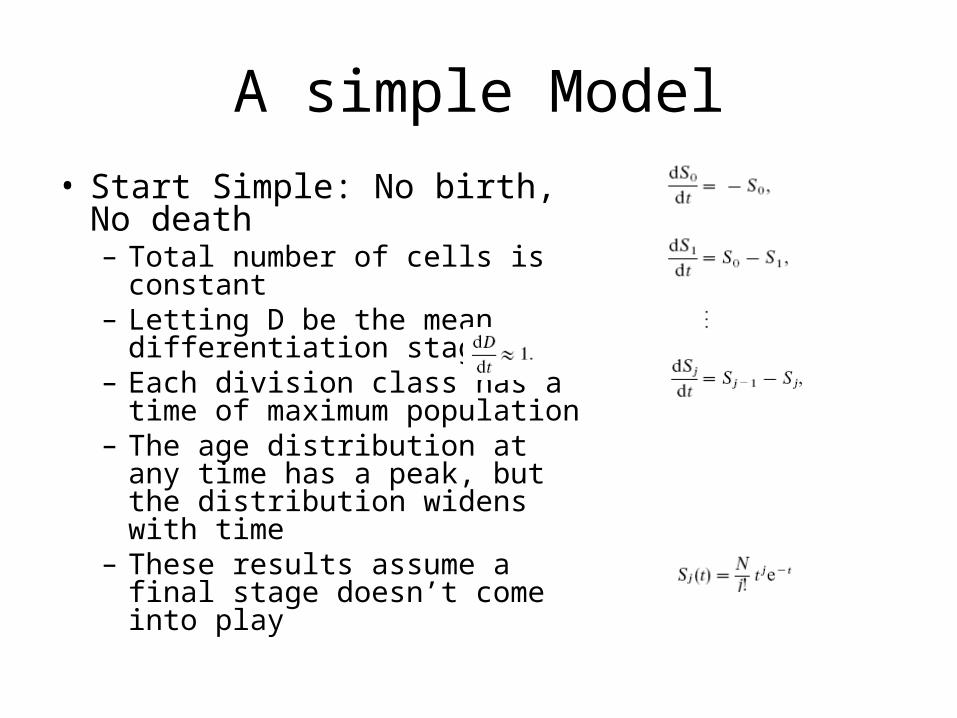
A simple Model

• Start Simple: No birth, No death– Total number of cells is

constant– Letting D be the mean

differentiation stage, – Each division class has a time

of maximum population– The age distribution at any time

has a peak, but the distribution widens with time

– These results assume a final stage doesn’t come into play

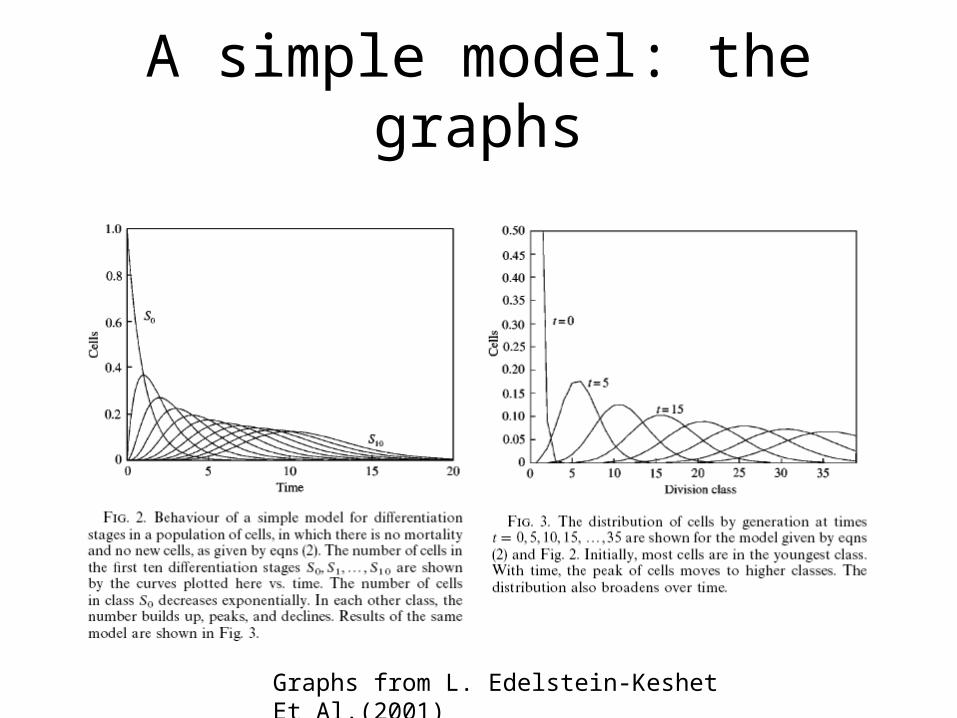
A simple model: the graphs

Graphs from L. Edelstein-Keshet Et Al.(2001)

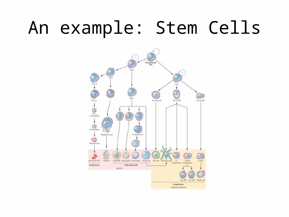
An example: Stem Cells

Telomeres

• Ends of chromosomes, containing repeats of (TTAGGG)

• Cell division results in decreased length– Humans lose 50-200 (average 100) bp

• Some cells (germline and some somatic cells) have telomerase or other mechanisms to avoid this loss

A model

• Add reproduction to our previous continous model

• “Death” is differentiation

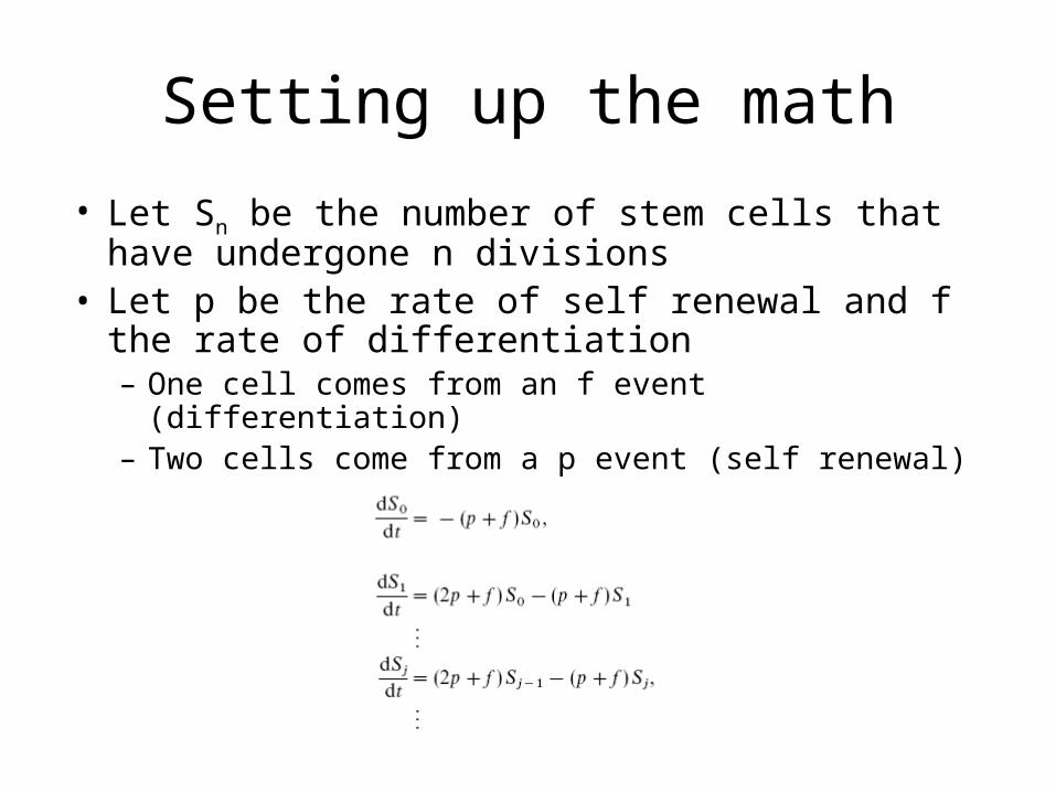
Setting up the math

• Let Sn be the number of stem cells that have undergone n divisions

• Let p be the rate of self renewal and f the rate of differentiation– One cell comes from an f event (differentiation)– Two cells come from a p event (self renewal)

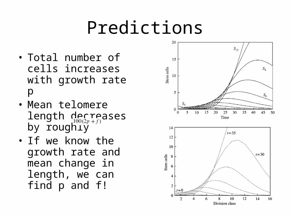
Predictions

• Total number of cells increases with growth rate p

• Mean telomere length decreases by roughly

• If we know the growth rate and mean change in length, we can find p and f!

Conclusions

• By slowly building models of aging up, we can make real predictions about our systems and also backtrack information out

• Models must ultimately move to non-linear regimes to better describe actual behavior

References

• Edelstein-Keshet, Leah, Aliza Esrael and Peter Lansdorp. “Modelling Perspectives on Aging: Can Mathematics Help us Stay Young?” 2001 Academic Press

• Caswell, H. (2001). Matrix Population Models: Construction, Analysis, and Interpretation, 2nd edn. Sunderland, MA: Sinauer Associates.

Images

• http://www.exploredesign.ca/blog/wp-content/uploads/2007/09/gollum.jpg

• www.srhc.com/babypics/Baby/pages/Images/baby.jpg

• http://www.robertokaplan.at/images/old-woman-madeira.jpg